Montevideo 13 Nov 2013 Current Trends in Advanced Process Control and Real-Time Optimization...

Montevideo13 Nov 2013

Current Trends in Advanced Process Control and Real-Time Optimization

Argimiro R. Secchi

Programa de Engenharia Química – COPPE

Centro de Tecnologia – UFRJ

Rio de Janeiro – RJ

2

OutlineOutline

• Advanced Process Control

• Model Predictive Control

• Modeling and Identification

• Real-Time Optimization

• Dynamic Real-Time Optimization

• Final Remarks

3

Basic ConceptsBasic Concepts

Advanced Process Control (APC): is a term that can include a

range of methodologies, including model predictive control

(MPC), fuzzy logic, statistical control, etc. The common objective

is to find a way to manage complex interactions within a process

better than traditional regulatory control.

4

Complex ProcessesComplex Processes

Plantwide control of transalkylation and disproportionation of toluene process (TADP)

* Klafke N., 2011. M.Sc. Thesis, Universidade Federal do Rio de Janeiro.

5

Process Control OverviewProcess Control Overview

Planning and Scheduling

Real-Time Optimization

Advanced Process Control

Regulatory Control

Process

Plantwide computer

Process computer

DSC

seconds

minutes

hours

weeks

6

Classical Process ControlClassical Process Control

0

11 ( )

t

c DI

deu k e t dt

dt

Lead / Lag filtersSwitchesMin, Max selectorsIf / Else logicsSequence logics

• Regulation

• Constraint handling

• Local optimization

ad hoc strategies

7

Example: Blending systemExample: Blending system

* J. H. Lee, 2005. Model Predictive Control. PASI, Iguazú, Argentina.

• Control rA and rB

• Control q if possible

• Flowrates of additives are limited

Classical solution

Setpoint

8

Model is not explicitly used inside the control algorithm

No clearly stated objective and constraints

Questionable performance

Complex control structure

Not robust to changes and failures

Focus on the performance of a local unit

Model is not explicitly used inside the control algorithm

No clearly stated objective and constraints

Questionable performance

Complex control structure

Not robust to changes and failures

Focus on the performance of a local unit

Classical SolutionClassical Solution

9

APC SolutionAPC Solution

1 2 3

2 2 2* * *

( ), ( ), ( ), , 1 1

min max

min ( | ) ( | ) ( | )

( ) , 1, 2,3 , , 1

1

P

A A B Bu j u j u jj k k M n

i i i

r k n k r r k n k r w q k n k q

u u j u i and j k k M

w

Prediction horizon

Control horizon

10

Classical vs. APC SolutionClassical vs. APC Solution

* T. Badgwell, 2003. Spring AIChE Meeting, New Orleans.

11

APC ObjectivesAPC Objectives

• Maximize production• Ensure product specifications• Minimize energy and water consumption• Minimize process variability• Minimize loss of products• Respect process constraints• Safeguard environmental laws

Constrained optimization problem

12

TimelineTimeline

* E. Almeida Nt, 2011. Ph.D. Thesis, UFRGS.

13

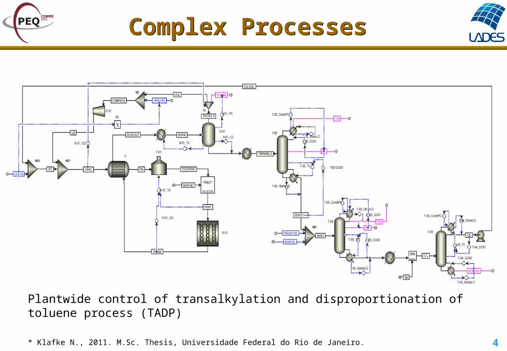
Open-Loop Optimal ControlOpen-Loop Optimal Control

Controller

Plant

set-point input output

r(t) u(t) y(t)

0

( )

0 0

min [ ( )] ( , , )

( , ) , ( )

( ) ( , )

( , ) 0

[ ( )] 0

ft

fu t

t

f f

x t x u r dt

dxf x u x t x

dty t h x u

g x u

g x t

model constraints

path constraints

terminal constraints

14

Open-loop optimal solution is not robust

Must be coupled with on-line state / model parameter update

Requires on-line solution for each updated problem

Analytical solution possible only in a few cases (LQ control)

Computational limitation for numerical solution

Open-loop optimal solution is not robust

Must be coupled with on-line state / model parameter update

Requires on-line solution for each updated problem

Analytical solution possible only in a few cases (LQ control)

Computational limitation for numerical solution

Open-Loop Optimal ControlOpen-Loop Optimal Control

Controller

Plant

set-point input output

r(t) u(t) y(t)

measurements

15

Model Predictive Control (MPC)Model Predictive Control (MPC)

Open-loop optimal control problem: Find current and future manipulated inputs that best meet a desired future output trajectory.

(desired output)

Feedback nature: Implement first “control move” then correct for model mismatch.

(desired output)

Major issue: disturbances vs. model uncertainty.* B.W. Bequette, 1998. Process Dynamics. Modeling, Analysis, and Simulation, Prentice Hall.

nex

t sa

mp

le t

ime

16

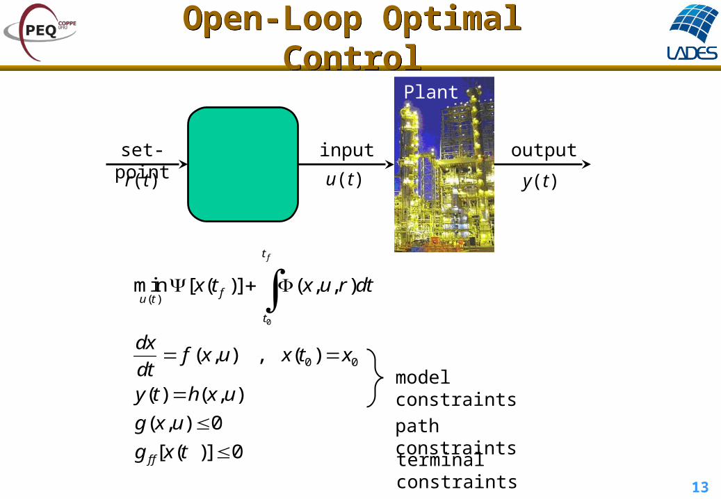
Open questions in MPCOpen questions in MPC

• Type of model for predictions?

linear: state space, TF, step response, impulse response, ARX

nonlinear: first principles, NN, Volterra, Wiener, Hammerstein,

multiple model, fuzzy, NARX

• Information needed at step k for predictions?

outputs, state estimates, measured disturbances, model parameters

• Objective function and optimization technique?

quadratic (QP), absolute values (LP), economics, nonlinear (NLP)

• Correction for model error?

additive output, disturbance estimation (KF, EKF, MHE)

17

Implementation of APCImplementation of APC

Control structure design

Check instrumentation and retune regulatory control

Pre-tests and design of inferences (soft sensors)

Plant test and identification of dynamic models

Controller configuration and closed-loop simulation

Commissioning and tuning of the controller

Monitoring the APC performance

Training of operators and documentation

18

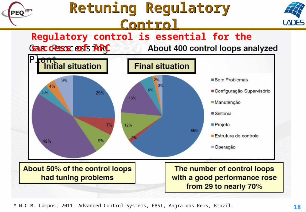
Retuning Regulatory ControlRetuning Regulatory Control

* M.C.M. Campos, 2011. Advanced Control Systems, PASI, Angra dos Reis, Brazil.

Gas Processing PlantRegulatory control is essential for the success of APC

19

Monitoring the APC PerformanceMonitoring the APC Performance

Changes in the unit operations

objectives;

Equipment efficiency losses

(fouling);

Changes in the feed quality;

Problems in instruments and in

soft sensors;

Lacks of qualified personnel for

the controller's maintenance.

MPC performance can degrade due to:

20

Linear MPC applicationsLinear MPC applications

* S.J. Qin, T.A. Badgwell, 2003. Control Engineering Practice,11, 733–764.

21

Nonlinear MPC applicationsNonlinear MPC applications


Non

linea

r S

tate

Spa

ceF

irst P

rinci

ples

Non

linea

r S

tate

Spa

ceN

eura

l Net

wor

ks

Line

ar A

RX

Sta

tic p

olyn

omia

ls

Non

linea

r S

tate

Spa

ceF

irst P

rinci

ples

Non

linea

r S

tate

Spa

ceF

irst P

rinci

ples

, NN

, …

Line

ar A

RX

Neu

ral N

etw

orks

Area AdersaAspen

TechnologyContinental

ControlsDOT

ProductsPavillion

Technologies TriSolutions Total

Air and Gas 18 18Chemicals 2 15 5 22Food Processing 9 9Polymers 1 5 15 1 22Pulp& Paper 1 1Refining 13 1 14Utilities 5 2 7Unclassified 1 1 2

Total 3 6 36 5 43 2 95

22

Evolution of LMPC TechnologyEvolution of LMPC Technology


Kalman (1960)

Linear Quadratic GaussianLinear state-space model

2 2

1

| 1 1| 1 1

| | 1 | 1

min

ˆ ˆ

ˆ ˆ ˆ

k jk j k jQ Ru

j

k k k k k

k k k k f k k k

x u

x A x B u

x x K y C x

|ˆk c k ku K x

23

LMPC GenerationsLMPC Generations

First Generation

•Identification and Command (IDCOM) Richalet et al. (1976, 1978); at Adersa Impulse response model Heuristic iterative algorithm

•Dynamic Matrix Control (DMC) Cutler & Ramaker (1979); at Shell in 70’s Step response model, LS solution

Second Generation

•QDMC Cutler, Morshedi & Haydel (1983), Garcia and Morshedi (1986)

Step response model Solution using QP

Third Generation

•IDCOM-M (Setpoint), HIECON (Adersa) Grosdidier et al. (1988) Multi-objective formulation (output | input) Soft, hard and ranked constraints

•SMOC (Shell Multivariable Opt. Control) Marquis & Broustail (1998) Bridge between state-space and MPC Disturbance model; KF

Fourth Generation

•DMC-plus, RMPCT Steady-state target optimization QP and economic objectives Model uncertainties Prioritized control objectives Graphical user interface

24

Weakness of LMPC GenerationsWeakness of LMPC Generations

First Generation

•Constraints handling on ad hoc basis

Second Generation

•No clear way to handle infeasible solution

•Weighted sum of objectives does not allow

the designer to reflect the true performance

requirements

Third Generation

•Limited model choices

•Poor user interfaces

Fourth Generation

•Finite horizon formulation does not inherit

strong stabilizing properties

•Lack of robust stability

25

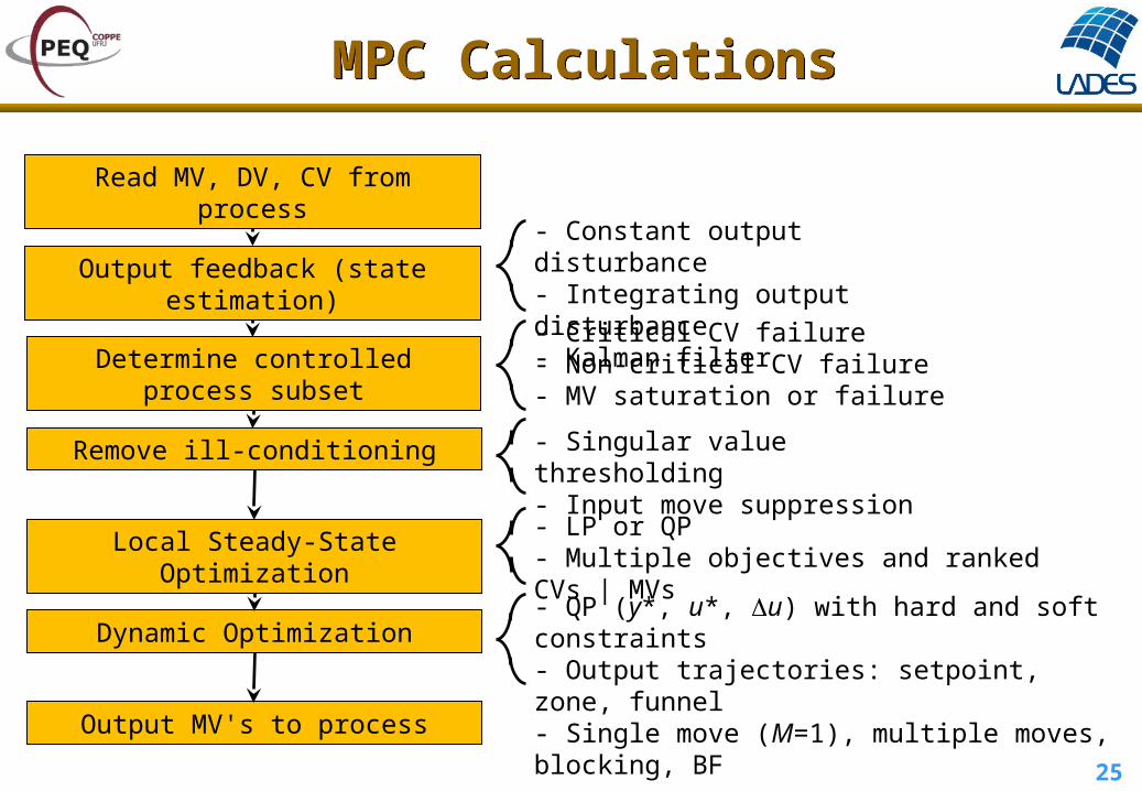
MPC CalculationsMPC Calculations

Read MV, DV, CV from process

Output feedback (state estimation)

Determine controlled process subset

Remove ill-conditioning

Local Steady-State Optimization

Dynamic Optimization

Output MV's to process

- Constant output disturbance- Integrating output disturbance- Kalman filter

- Critical CV failure- Non-critical CV failure- MV saturation or failure

- Singular value thresholding- Input move suppression

- LP or QP- Multiple objectives and ranked CVs | MVs

- QP (y*, u*, u) with hard and soft constraints- Output trajectories: setpoint, zone, funnel- Single move (M=1), multiple moves, blocking, BF

26

Dynamic OptimizationDynamic Optimization

1

1

, ,1 0

1 1

maxmin

maxmin

maxmin

min

, , 1, ,

, , 1, ,

, 0 , 1, ,

, 0, , 1

, 0, ,

jj jk k M

P Mq qq qy u

k j j k j k jT RQ Ru uj j

k j k j k j

k j k j k j

j k j j j

k j

k j

e s e u

x f x u j P

y h x u j P

y s y y s s j P

u u u j M

u u u j

1M

y rk j k j k j

uk j k j s

e y y

e u u

where

error from desired steady state input (us)

error from desired output trajectory (yr)

27

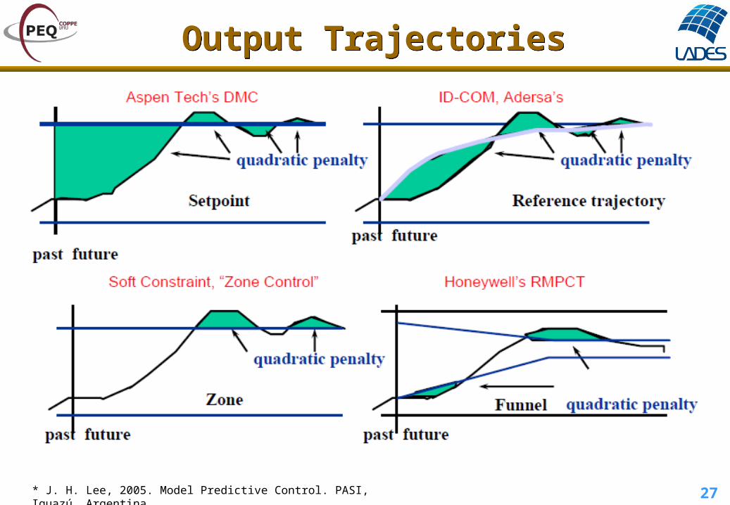
Output TrajectoriesOutput Trajectories

* J. H. Lee, 2005. Model Predictive Control. PASI, Iguazú, Argentina.

28

HorizonsHorizons

Prediction horizon (P) Control horizon (M)

Man

ipul

ated

Var

iabl

e

Man

ipul

ated

Var

iabl

e

Man

ipul

ated

Var

iabl

e

Man

ipul

ated

Var

iabl

e

Base Functions

(with blocking)

29

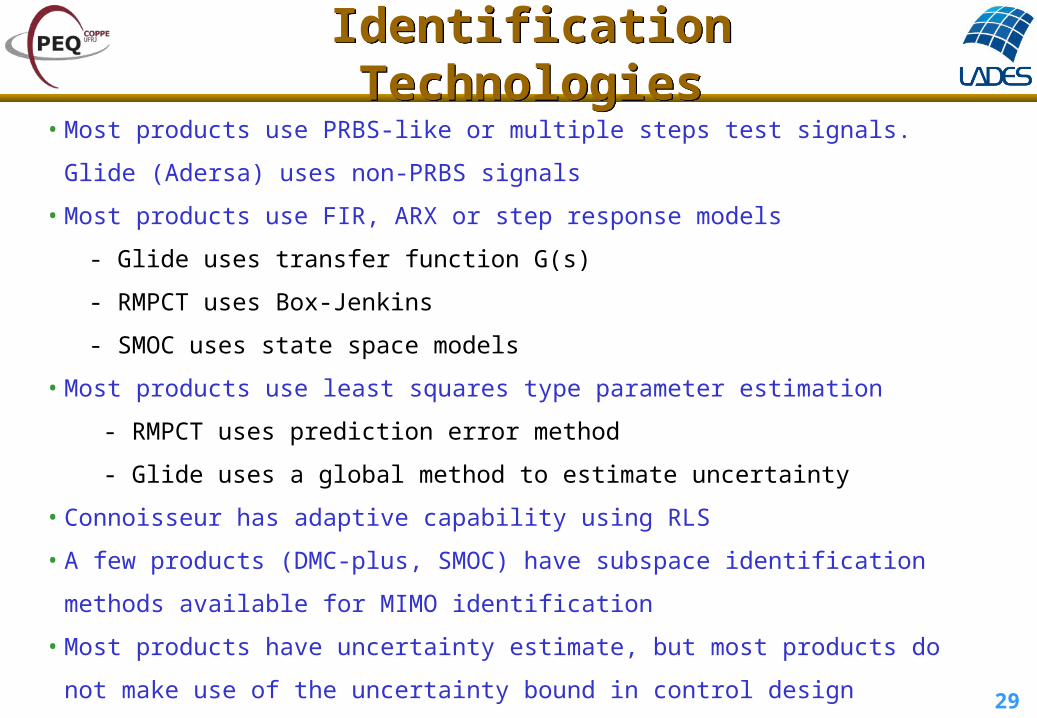
Identification TechnologiesIdentification Technologies• Most products use PRBS-like or multiple steps test signals. Glide (Adersa) uses non-

PRBS signals

• Most products use FIR, ARX or step response models

- Glide uses transfer function G(s)

- RMPCT uses Box-Jenkins

- SMOC uses state space models

• Most products use least squares type parameter estimation

- RMPCT uses prediction error method

- Glide uses a global method to estimate uncertainty

• Connoisseur has adaptive capability using RLS

• A few products (DMC-plus, SMOC) have subspace identification methods available for

MIMO identification

• Most products have uncertainty estimate, but most products do not make use of the

uncertainty bound in control design

30

Challenges for MPCChallenges for MPC

Optimization problem - infinite prediction horizon - multiple objectives

Simplifying the model development process - plant testing & system identification - nonlinear model development - intensive use of dynamic simulators - model reduction techniques

State Estimation - Lack of sensors and sensor location for key variables

Reducing computational complexity - approximate solutions, preferably with some guaranteed properties - modern computation (sparse matrices, better numerical methods)

Better management of “uncertainty” - creating models with uncertainty information (e.g., stochastic model) - on-line estimation of parameters / states - “robust” solution of optimization - self-tuning and adaptive MPC

31

Real-Time Optimization (RTO)Real-Time Optimization (RTO)

Planning & Scheduling

32

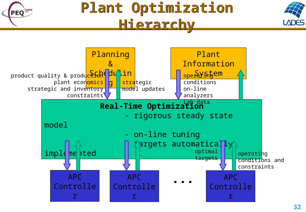
Plant Optimization HierarchyPlant Optimization Hierarchy

APC Controller

Real-Time Optimization - rigorous steady state model - on-line tuning - targets automatically implemented

Planning & Scheduling

Plant Information System

product quality & productionplant economics

strategic and inventory constraintsstrategic model updates

operating conditionson-line analyzersLab data

optimal targets

operating conditions and constraints

APC Controller

APC Controller

33

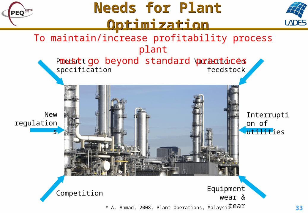
Needs for Plant OptimizationNeeds for Plant Optimization

Product specification

New regulations

Competition

Variation in feedstock

Interruption of utilities

Equipment wear & tear

To maintain/increase profitability process plantmust go beyond standard practices

* A. Ahmad, 2008, Plant Operations, Malaysia.

34

Potentials for OptimizationPotentials for Optimization

Sales limited by production - Plant throughput should be increased

Sales limited by market - Plant efficiency must be improved

Large throughputs - Small savings in productivity costs are greatly magnified

High raw material or energy consumption - Mass or heat integration should be analyzed

Losses of valuable or hazardous components through waste streams - Mass exchange network should be optimized

Product quality over specified - Plant should operate near constraints

35

RTO CalculationsRTO Calculations

Plant data Gross error detection

wait

Data reconciliation

Model updating

Steady state optimization

APC targets Solution implementation

Yes

Yes

No

No

36

Successful RTO Requires APCSuccessful RTO Requires APC

Optimal operating conditions often located near constraints - Benefits are achieved by consistently pushing the process to the most profitable constraints

Traditional PID-type constraint-selector controllers give poor performance against multiple constraints

- Pairing of constraints and manipulated variables is fixed in controller design - Retuning needed as constraints change

MPC are designed to run at multiple constraints - Predictive nature allows constrained variables to be corrected before they

reach the constraints

37

APC and RTO BenefitsAPC and RTO Benefits

0

20

40

60

80

100

0 20 40 60 80 100

Inve

stm

ent (

%)

Potential (%)

RTOAPC

DCS

ARC

Regulatory Control: DCS + ARC (Advanced Regulatory Control)

38

Steady state detection is necessary before optimization

Large-scale problems require high computational demand

The same steady state is needed when implementing the targets

Large set-point changes should be avoided for safety reasons

RTO LimitationsRTO Limitations

39

Besl et al. (1998) – RTO system that do not wait for steady state.

Cheng & Zafiriou (2000) – simultaneous optimization and model updating.

Becerra et al. (1998); Nath & Alzein (2000); Tvrzská & Odloak (1998) – Economic objectives in the MPC (one-layer RTO+APC).

Sorensen & Cutler (1998); Rao & Rawlings (1999); Qin & Badgwell (1997); Ying et al. (1999) – RTO results are sent to a local steady state optimizer (LP or QP) coupled to the MPC.

Efforts to Circumvent RTO LimitationsEfforts to Circumvent RTO Limitations

40

RTO

LP – QP Steady state target

calculation

-----------------------------

MPC

SS target Measures / disturbances

Process

Set-points Measures

Alternative RTO FormulationsAlternative RTO Formulations

RTO with target calculation

LP – QP Steady state target

and economic calculation

-----------------------------

MPC

SS target Measures / disturbances

Process

One-layer RTO+APC

41

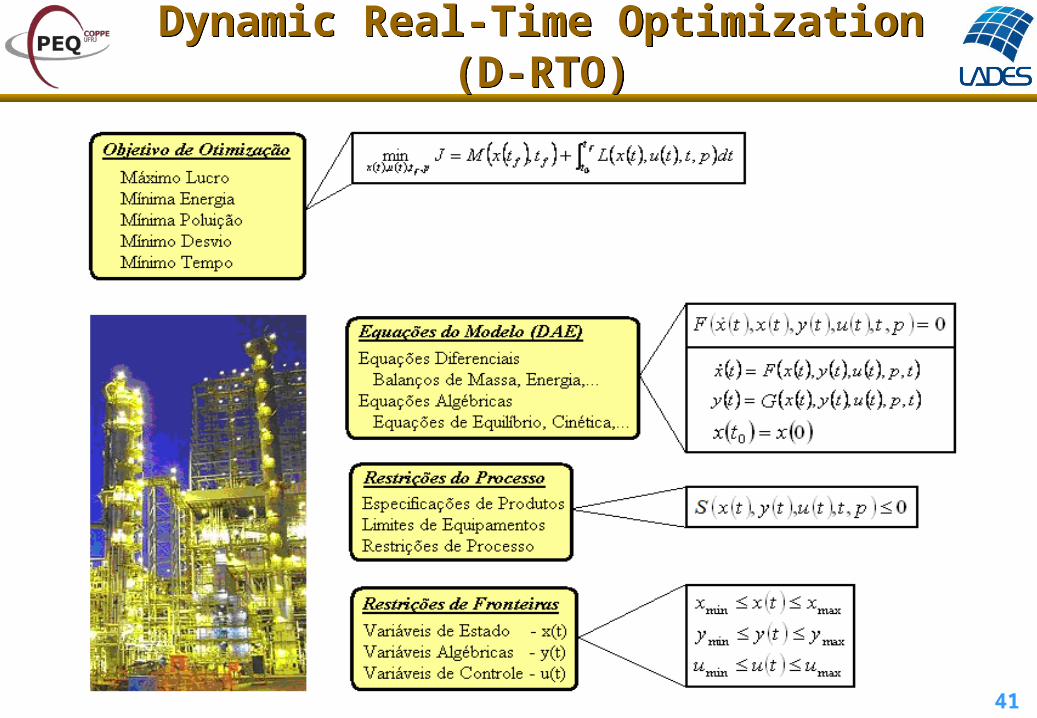
Dynamic Real-Time Optimization (D-RTO)Dynamic Real-Time Optimization (D-RTO)

42

Process + Regulatory Control

MPC

D-RTO / RTO

data pre-processing and dynamic data

reconciliation

model updating for RTO / D-RTO

model updating for LMPC / NMPC

Production Planing

inferences

u(t)y(t)

Y(t)

u*(t)y*(t)

feed specification, product and market

Model server(rigorous, empiric, hybrid, reduced)

d(t)

RTO vs. D-RTO, LMPC vs. NMPCRTO vs. D-RTO, LMPC vs. NMPC

43

Alternative D-RTO FormulationsAlternative D-RTO Formulations

Plant – Regulatory Control

State Estimator

D-RTO

x u

x u^ ^

u

Production Scheduling Information

Plant– Regulatory Control

State Estimator

D-RTO

x u u


Time- scale

separator

MPC

xref uref

x u~ ~

x u_ _

x u^ ^

One layer Two layers

44



State Estimator

D-RTO

x u u


Time- scale

separator

MPC

xref uref

x u~ ~

x u_ _

x u^ ^

Time-scale separators


D-RTO

x u u


Large time-scale estimator

LMPC

xref uref

x u_ _


D-RTO

x u u


Time- scale

separator

NMPC

xref uref

x u~ ~

x u_ _

x u^ ^

Large time-scale

estimator

Short time-scale

estimator x u ~ ~

* Kadam et al., 2002; Helbig et al., 2000.

45


State Estimator

D-RTO

x uu


Time-scale separator

MPC

xref uref

x u~ ~

x u_ _

x u^ ^

Result validation


State Estimator

D-RTO

x u u


D-RTO Trigger

MPC

xref uref

x u~ ~

x u_ _

x u^ ^


Result validation D-RTO Trigger

* Kadam & Marquardt, 2004.

46


D-RTO with infeasibilities treatment

* Ameida & Secchi, 2012.

, , , , ,

0 0 0

0

0

2

2

min

. .

, , , , , 0 , ,

, 0

( - utopic value of objective function)

1, ,

1, ,

x y u fu s s s p

f

L Lf f

xi

xi

yj

yj

uk

t

s t

F x t x t y t u t p t x t x t t t

dt t

dt

x t t w

s tt where i nx

s tt where j ny

s t

2

1, ,

x

y

u

uk

L x U

L y U

L u U

Sx x x xL U

Sy yy yL U

Su u u uL U

t where k nu

x x t s t x

y y t s t y

u u t s t u

s s t s where s t

s s t s where s t

s s t s where s t

4747

Dynamic Optimization MethodsDynamic Optimization Methods

52

• Piecewise Constant Function

• Piecewise Linear Function

Control ParameterizationControl Parameterization

53

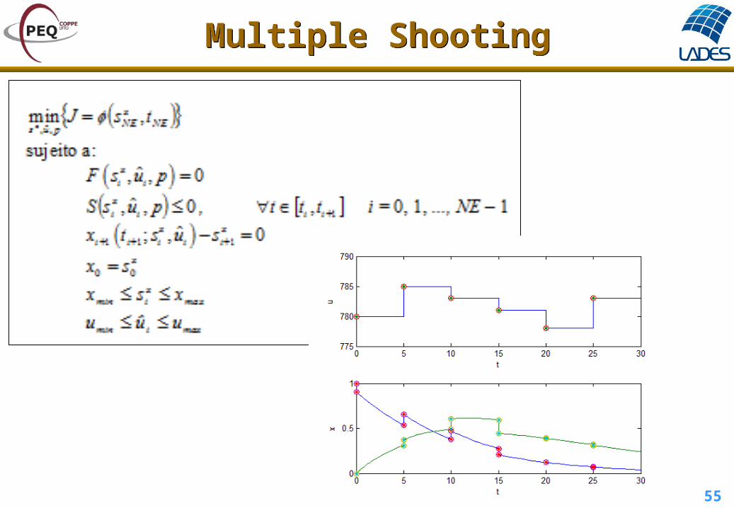
• Partial Discretization (Sequential Methods) – Single shooting (Pollard & Sargent, 1970; Sargent & Sullivan, 1977)

– Multiple shooting (Bock & Plitt, 1984)

• Full Discretization (Simultaneous Methods) – Orthogonal Collocation on Finite Elements (Cuthrell & Biegler, 1987)

Numerical MethodsNumerical Methods

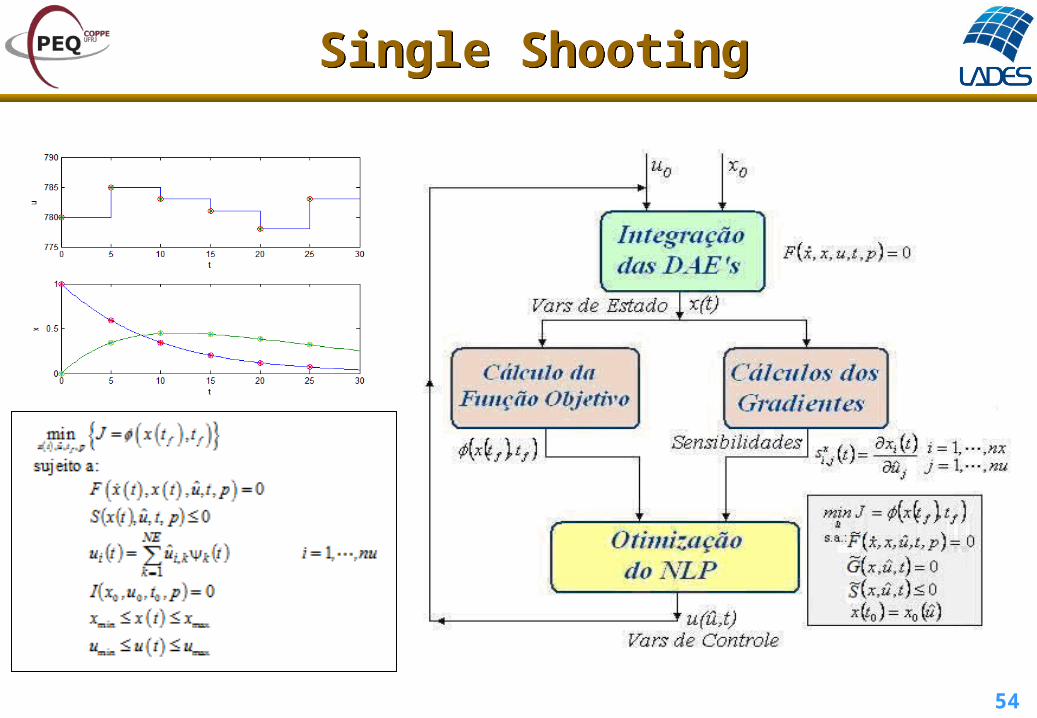
54

Single ShootingSingle Shooting

55

Multiple ShootingMultiple Shooting

56

Orthogonal Collocation on Finite ElementsOrthogonal Collocation on Finite Elements

57

Orthogonal Collocation on Finite ElementsOrthogonal Collocation on Finite Elements

59

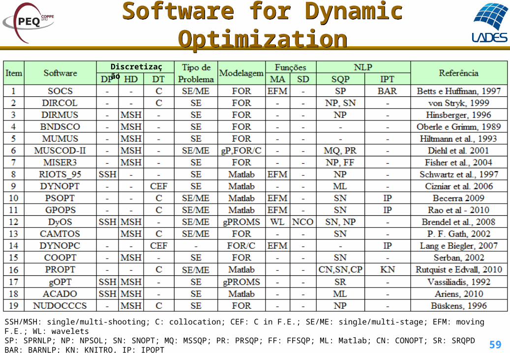
Software for Dynamic OptimizationSoftware for Dynamic Optimization

SSH/MSH: single/multi-shooting; C: collocation; CEF: C in F.E.; SE/ME: single/multi-stage; EFM: moving F.E.; WL: waveletsSP: SPRNLP; NP: NPSOL; SN: SNOPT; MQ: MSSQP; PR: PRSQP; FF: FFSQP; ML: Matlab; CN: CONOPT; SR: SRQPDBAR: BARNLP; KN: KNITRO, IP: IPOPT

Discretização

60

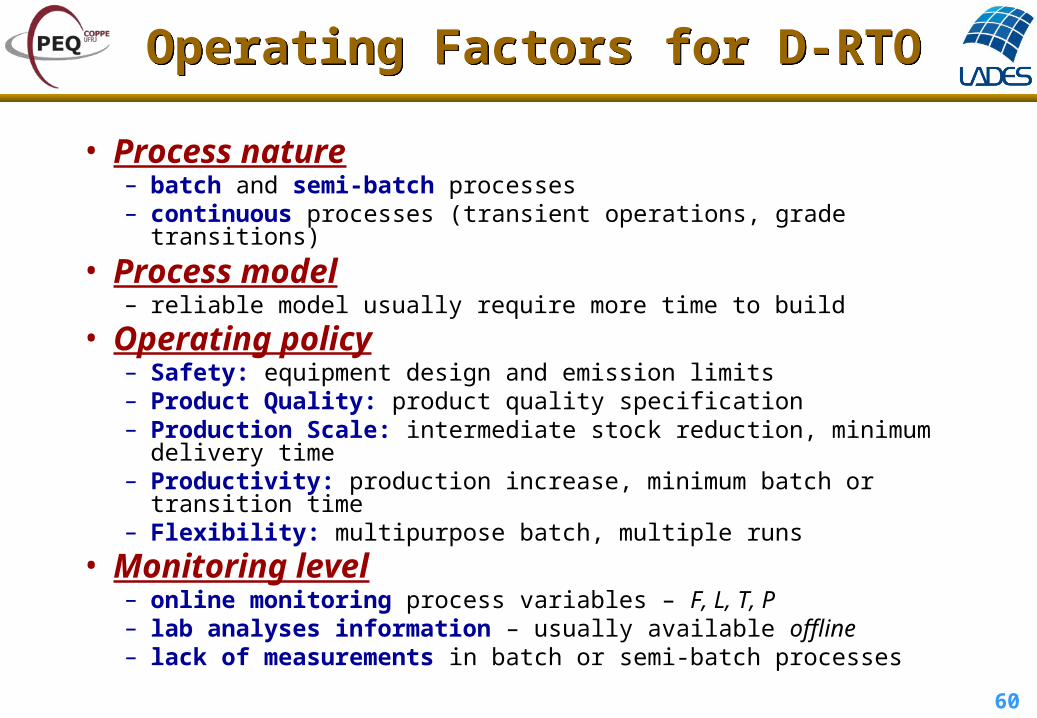
• Process nature – batch and semi-batch processes – continuous processes (transient operations, grade transitions)

• Process model– reliable model usually require more time to build

• Operating policy – Safety: equipment design and emission limits– Product Quality: product quality specification– Production Scale: intermediate stock reduction, minimum delivery time – Productivity: production increase, minimum batch or transition time– Flexibility: multipurpose batch, multiple runs

• Monitoring level – online monitoring process variables – F, L, T, P– lab analyses information – usually available offline – lack of measurements in batch or semi-batch processes

Operating Factors for D-RTOOperating Factors for D-RTO

61

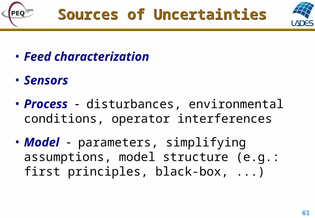
• Feed characterization

• Sensors

• Process disturbances, environmental conditions, operator interferences

• Model parameters, simplifying assumptions, model structure (e.g.: first principles, black-box, ...)

Sources of UncertaintiesSources of Uncertainties

62

• Nominal Optimization– uncertainties not taken into account

– offline

• Optimization with uncertainties – robust optimization (Terwiesch et al., 1994) uncertainties are taken into

account without model updating and state estimation

– measure-based optimization - MBO (Srinivasan & Bonvin, 2007)• explicit optimization: model updating and state estimation based on plant

measurements (NMPC - Biegler & Zavala, 2009; DRTO - Kadam et al., 2004)

• implicit optimization: structure detection based on necessary condition of optimality (NCO - Srinivasan et al., 2002).

Type of OptimizationType of Optimization

63

• Mesh adaptation

• Element grouping

• Structure detection

• Optimizer trigger

• NLP solvers

Optimization FeaturesOptimization Features

Sequential (Betts & Huffman, 1998)

Simultaneous (Tanartkit & Biegler, 1997) Multi-scale (Binder et al. 1997; Santos et al., 2012)

64

• Mesh adaptation




• NLP solvers


* Lang & Biegler, 2005.

65

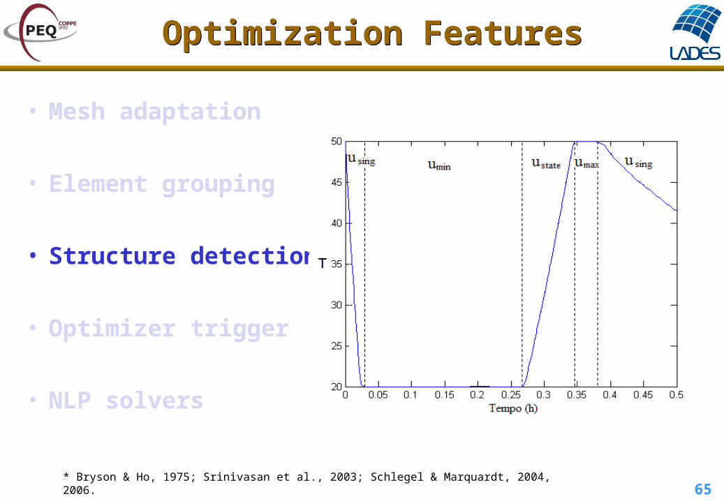
• Mesh adaptation




• NLP solvers


* Bryson & Ho, 1975; Srinivasan et al., 2003; Schlegel & Marquardt, 2004, 2006.

66

• Mesh adaptation




• NLP solvers


* Kadam et al., 2002.

x u_ _

x u

x u^ ^


State Estimator

D-RTO

x u u


D-RTO Trigger

MPC

xref uref

~ ~

67

• Mesh adaptation




• NLP solvers


Sequential (Pollard & Sargent, 1970)

Multiple-Shooting (Bock & Plitt, 1984) Simultaneous (Cuthrell & Biegler, 1987)

68

DRTO NMPCApplication batch or continuous process

optimizer for recipe changesplant controller to track set-point changes

Plant feedback less frequent state estimation model update for fast predictions

Run time minutes seconds

Optimization horizon long (up to days) short (up to hours)

Model reliable for long predictions may be simplified for short predictions

Example: Inline blending

search for optimal recipe – minimizing final time and deviations from product specification.

reject disturbances while tracking optimal recipe.

D-RTO vs. NMPCD-RTO vs. NMPC

69

Challenges for D-RTOChallenges for D-RTO

Real-time system - full integration of all parts (dynamic data reconciliation, state and

parameter estimation, inferences, dynamic optimization, APC) - better integration with scheduling and planning layers - robust solvers - fast solving of infeasibilities

Model development and updating - nonlinear model development and model reduction - parameter selection for estimation (Identifiability) - subspace state estimation - uncertainty management

Solution refinement and size reduction - fast mesh adaptation - structure detection integrated with mesh refinement - element grouping

Computational resources - parallel computing (clusters, GPU)

70

Final RemarksFinal Remarks

• LMPC and RTO are mature industrial technologies

• NMPC and D-RTO are emerging industrial technologies

• Robustness and efficiency are still very demanding

• Monitoring and diagnosis are open issues for feedback information

• First principles dynamic models are even more needed

Lots of work for Process System Engineers!!

71

... thank you for your attention!

Laboratório de Modelagem, Simulação e Controle de Laboratório de Modelagem, Simulação e Controle de ProcessosProcessos

• Prof. Argimiro Resende Secchi, D.Sc.Prof. Argimiro Resende Secchi, D.Sc.

• Phone: +55-21-2562-8307Phone: +55-21-2562-8307

• E-mail: [email protected]: [email protected]• http://www.peq.coppe.ufrj.br/Areas/Modelagem_e_simulacao.htmlhttp://www.peq.coppe.ufrj.br/Areas/Modelagem_e_simulacao.html

http://www.enq.ufrgs.br/alsoc

Montevideo 13 Nov 2013 Current Trends in Advanced Process Control and Real-Time Optimization...

Documents

Transcript of Montevideo 13 Nov 2013 Current Trends in Advanced Process Control and Real-Time Optimization...