1

MIT EECS 6.837

Monte-Carlo Ray Tracing

MIT EECS 6.837

Last Time?• Two perspective on antialiasing:

– Signal processing– Integration

• Supersampling, multisampling• Jittering, Poisson disk• Adaptive supersampling• Monte-Carlo integration• Probabilities: discrete, continuous

– Expected value, variance

MIT EECS 6.837

Goal today• Prove that Monte-Carlo integration works

– Notion of expected value• Prove its convergence speed

– Error: notion of variance• For all this, we need to study what happens to

expected value and variance when we had tons of random samples

• Apply to ray tracing

MIT EECS 6.837

Today’s lecture• Expected value and variance• Analysis of Monte-Carlo integration• Monte-Carlo in graphics• Importance sampling• Stratified sampling• Global illumination• Advanced Monte-Carlo rendering

MIT EECS 6.837

A little bit of eye candy for motivation

• Glossy material rendering• Random reflection rays around mirror direction

– 1 sample per pixel

MIT EECS 6.837

A little bit of eye candy for motivation

• Glossy material rendering• Random reflection rays around mirror direction

– 256 sample per pixel

2

MIT EECS 6.837

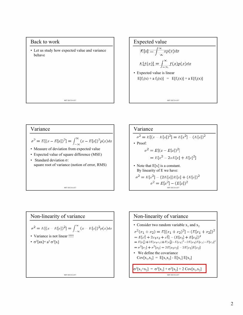
Back to work• Let us study how expected value and variance

behave

MIT EECS 6.837

Expected value

• Expected value is linear E[f1(x) + a f2(x)] = E[f1(x)] + a E[f2(x)]

MIT EECS 6.837

Variance

• Measure of deviation from expected value• Expected value of square difference (MSE)• Standard deviation σ:

square root of variance (notion of error, RMS)

MIT EECS 6.837

Variance

• Proof:

• Note that E[x] is a constant. By linearity of E we have:

MIT EECS 6.837

Non-linearity of variance

• Variance is not linear !!!!• σ2[ax]= a2 σ2[x]

MIT EECS 6.837

Non-linearity of variance• Consider two random variable x1 and x2

• We define the covarianceCov[x1,x2] = E[x1x2] - E[x1] E[x2]

σ2[x1+x2] = σ2[x1] + σ2[x2] + 2 Cov[x1,x2]

3

MIT EECS 6.837

Non-linearity of variance, covariance• Consider two random variable x1 and x2

• We define the covarianceCov[x1,x2] = E[x1x2] - E[x1] E[x2]– Tells how much they are big at the same time– Null if variables are independent

σ2[x1+x2] = σ2[x1] + σ2[x2] + 2 Cov[x1,x2]

MIT EECS 6.837

Recap• Expected value is linear

– E[ax1+bx2]=aE[x1]+bE[x2]• Variance is not• For two independent variables

– σ2[x1+x2]=σ2[x1]+σ2[x2]– If not independent, needs covariance

• σ2[ax]=a2σ2[x]

MIT EECS 6.837

Questions?• Image from the ARNOLD Renderer by Marcos Fajardo

MIT EECS 6.837

Today’s lecture• Expected value and variance• Analysis of Monte-Carlo integration• Monte-Carlo in graphics• Importance sampling• Stratified sampling• Global illumination• Advanced Monte-Carlo rendering

MIT EECS 6.837

Monte Carlo integration • Function f(x) of x ∈ [a b] • We want to compute

• Consider a random variable x• If x has uniform distribution, I=E[f(x)]

– By definition of the expected value

MIT EECS 6.837

Sum of Random Variables• Use N independent identically-distributed (IID)

variables xi– Share same probability (uniform here)

• Define

• By linearity of the expectation:E[FN] = E[f(x)]

4

MIT EECS 6.837

Study of variance

• Recall σ2[x+y] = σ2[x] + σ2[y] + 2 Cov[x,y]– We have independent variables: Cov[xi, xj]=0 if i ≠ j

• σ2[ax] = a2 σ2[x]

• i.e. stddev σ (error) decreases by MIT EECS 6.837

Example

• We know it should be 1.0

• In practicewith uniform samples:

N

σ2

- σ2

error

MIT EECS 6.837

Monte Carlo integration with proba• Consider N random samples over domain

with probability p(x)• Define estimator h I i as:

• Probability p allows us to sample the domain more smartly

MIT EECS 6.837

Monte-Carlo Recap• Expected value is the integrand

– Accurate “on average”• Variance decrease in 1/N

– Error decreases in

• Good news:– Math are over for today– OK, it’s bad news if you like math

(and you should)

MIT EECS 6.837

Questions?

MIT EECS 6.837

Advantages of MC Integration• Few restrictions on the integrand

– Doesn’t need to be continuous, smooth, ...– Only need to be able to evaluate at a point

• Extends to high-dimensional problems– Same convergence

• Conceptually straightforward• Efficient for solving at just a few points

5

MIT EECS 6.837

Disadvantages of MC• Noisy• Slow convergence• Good implementation is hard

– Debugging code– Debugging maths– Choosing appropriate techniques

MIT EECS 6.837

Questions?• Images by Veach and Guibas

Naïve sampling strategy Optimal sampling strategy

MIT EECS 6.837

Today’s lecture• Expected value and variance• Analysis of Monte-Carlo integration• Monte-Carlo in graphics• Importance sampling• Stratified sampling• Global illumination• Advanced Monte-Carlo rendering

MIT EECS 6.837

What can we integrate?• Pixel: antialiasing• Light sources: Soft shadows• Lens: Depth of field• Time: Motion blur• BRDF: glossy reflection• Hemisphere: indirect lighting

MIT EECS 6.837

Domains of integration• Pixel, lens (Euclidean 2D domain)• Time (1D)• Hemisphere

– Work needed to ensure uniform probability• Light source

– Same thing: make sure that the probabilities and the measures are right.

MIT EECS 6.837

Example: Light source• Integrate over surface or over angle• Be careful to get probabilities and integration

measure right!– More in 6.839

source

hemisphere

Sampling the source uniformly Sampling the hemisphere uniformly

6

MIT EECS 6.837

Questions?• Image by Henrik

MIT EECS 6.837

Today’s lecture• Expected value and variance• Analysis of Monte-Carlo integration• Monte-Carlo in graphics• Importance sampling• Stratified sampling• Global illumination• Advanced Monte-Carlo rendering

MIT EECS 6.837

Important issues in MC renderingReduce variance!• Choose a smart probability distribution• Choose smart sampling patterns

And of course, cheat to make it faster without being noticed

MIT EECS 6.837

Example: Glossy rendering• Integrate over hemisphere• BRDF times cosine times incoming light

)( iωI

Slide courtesy of Jason Lawrence

MIT EECS 6.837

Sampling a BRDF

5 Samples/Pixel

oω)(U iω

)(P iωoω

Slide courtesy of Jason Lawrence MIT EECS 6.837

Sampling a BRDF

25 Samples/Pixel

)(U iωoω

)(P iωoω

Slide courtesy of Jason Lawrence

7

MIT EECS 6.837

Sampling a BRDF

75 Samples/Pixel

)(U iωoω

)(P iωoω

Slide courtesy of Jason Lawrence MIT EECS 6.837

Importance sampling

• Choose p wisely to reduce variance– p that resembles f– Does not change convergence rate (still sqrt)– But decreases the constant

uniformbad good

MIT EECS 6.837

Questions?

Traditional importance functionTraditional importance function Better importance by Lawrence et al. Better importance by Lawrence et al.

1200 Samples/Pixel

MIT EECS 6.837

Today’s lecture• Expected value and variance• Analysis of Monte-Carlo integration• Monte-Carlo in graphics• Importance sampling• Stratified sampling• Global illumination• Advanced Monte-Carlo rendering

MIT EECS 6.837

Stratified sampling• With uniform sampling, we can get unlucky

– E.g. all samples in a corner• To prevent it, subdivide domain Ω

into non-overlapping regions Ωi– Each region is called a stratum

• Take one random samples per Ωi

MIT EECS 6.837

Example• Borrowed from Henrik Wann Jensen

Unstratified Stratified

8

MIT EECS 6.837

Stratified sampling - bottomline• Cheap and effective• Typical example: jittering for antialiasing

– Signal processing perspective: better than uniform because less aliasing (spatial patterns)

– Monte-Carlo perspective: better than random because lower variance (error for a given pixel)

MIT EECS 6.837

Questions?• Image from the ARNOLD Renderer by Marcos Fajardo

MIT EECS 6.837

Today’s lecture• Expected value and variance• Analysis of Monte-Carlo integration• Monte-Carlo in graphics• Importance sampling• Stratified sampling• Global illumination• Advanced Monte-Carlo rendering

MIT EECS 6.837

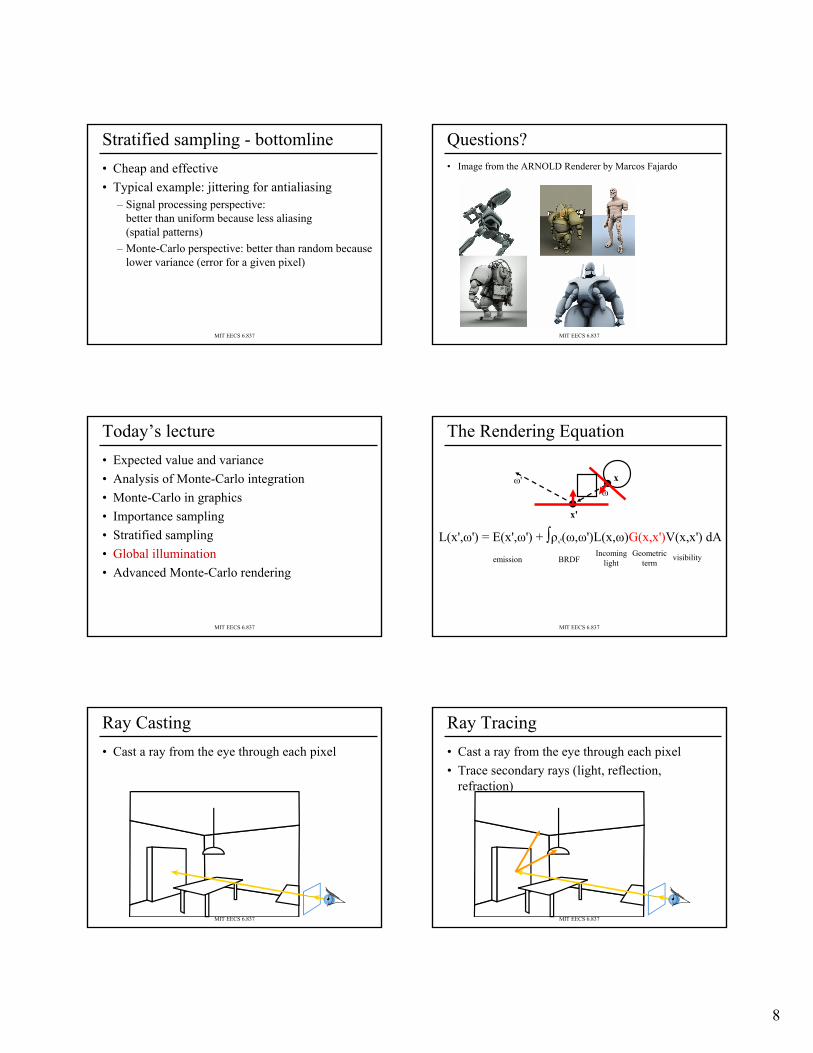
The Rendering Equation

x'

ω'ω

x

L(x',ω') = E(x',ω') + ∫ρx'(ω,ω')L(x,ω)G(x,x')V(x,x') dAemission BRDF

Incominglight

Geometricterm

visibility

MIT EECS 6.837

Ray Casting• Cast a ray from the eye through each pixel

MIT EECS 6.837

Ray Tracing• Cast a ray from the eye through each pixel • Trace secondary rays (light, reflection,

refraction)

9

MIT EECS 6.837

Monte-Carlo Ray Tracing• Cast a ray from the eye through each pixel• Cast random rays from the visible point

– Accumulate radiance contribution

MIT EECS 6.837

Monte-Carlo Ray Tracing• Cast a ray from the eye through each pixel• Cast random rays from the visible point • Recurse

MIT EECS 6.837

Monte-Carlo• Cast a ray from the eye through each pixel• Cast random rays from the visible point • Recurse

MIT EECS 6.837

Monte-Carlo• Systematically sample primary light

MIT EECS 6.837

Results

MIT EECS 6.837

Monte Carlo Path Tracing• Trace only one secondary ray per recursion• But send many primary rays per pixel• (performs antialiasing as well)

10

MIT EECS 6.837

Results• 10 paths/pixel

Think about it : we compute an infinite-dimensional integral with 10 samples!!!

MIT EECS 6.837

Results: glossy• 10 paths/pixel

MIT EECS 6.837

Results: glossy• 100 paths/pixel

MIT EECS 6.837

Importance of sampling the lightWithout explicit

light samplingWith explicit light sampling

1 path per pixel

4 path per pixel

MIT EECS 6.837

Why use random numbers?• Fixed random sequence• We see the structure in the error

MIT EECS 6.837

Convergence speed

11

MIT EECS 6.837

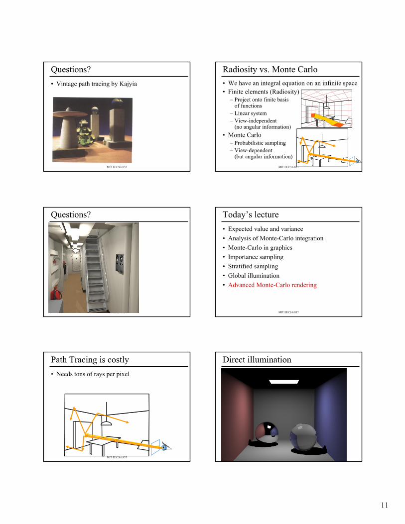
Questions?• Vintage path tracing by Kajyia

MIT EECS 6.837

Radiosity vs. Monte Carlo• We have an integral equation on an infinite space• Finite elements (Radiosity)

– Project onto finite basis of functions

– Linear system– View-independent

(no angular information)• Monte Carlo

– Probabilistic sampling– View-dependent

(but angular information)

MIT EECS 6.837

Questions?

MIT EECS 6.837

Today’s lecture• Expected value and variance• Analysis of Monte-Carlo integration• Monte-Carlo in graphics• Importance sampling• Stratified sampling• Global illumination• Advanced Monte-Carlo rendering

MIT EECS 6.837

Path Tracing is costly• Needs tons of rays per pixel

MIT EECS 6.837

Direct illumination

12

MIT EECS 6.837

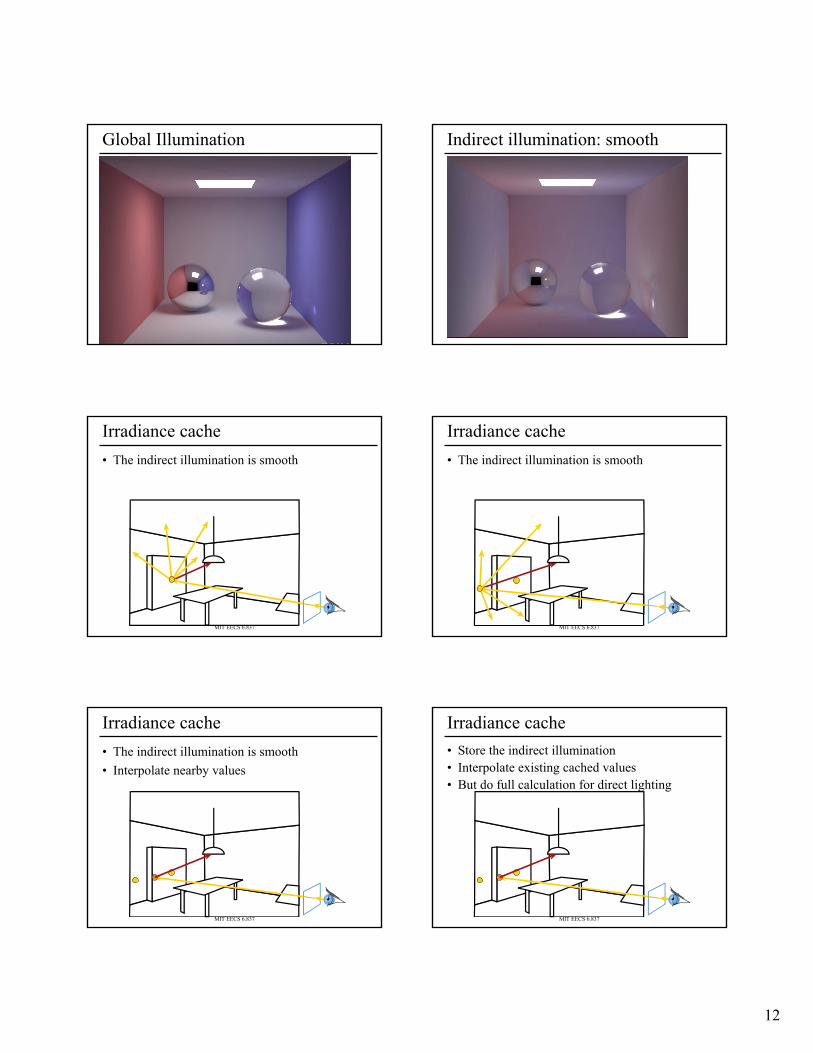
Global Illumination

MIT EECS 6.837

Indirect illumination: smooth

MIT EECS 6.837

Irradiance cache• The indirect illumination is smooth

MIT EECS 6.837

Irradiance cache• The indirect illumination is smooth

MIT EECS 6.837

Irradiance cache• The indirect illumination is smooth• Interpolate nearby values

MIT EECS 6.837

Irradiance cache• Store the indirect illumination• Interpolate existing cached values• But do full calculation for direct lighting

13

MIT EECS 6.837

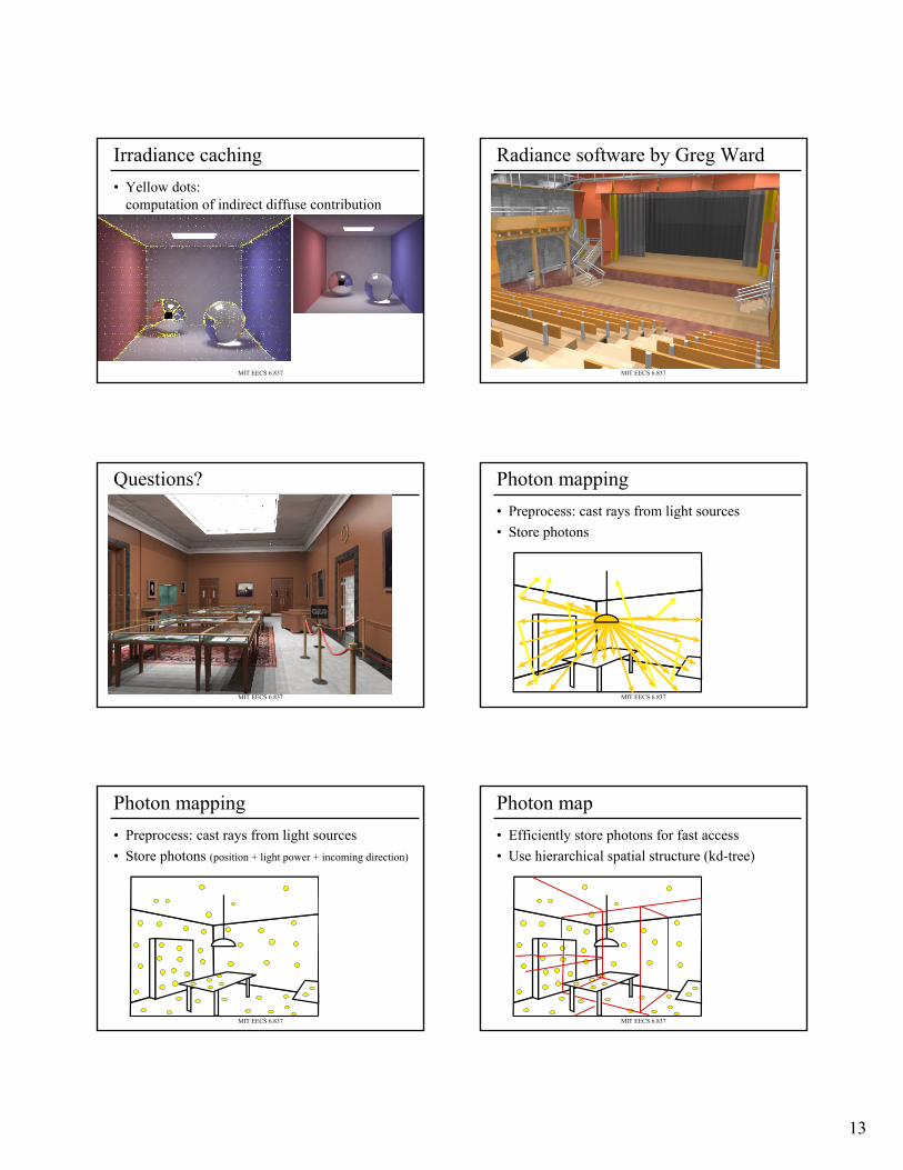
Irradiance caching• Yellow dots:

computation of indirect diffuse contribution

MIT EECS 6.837

Radiance software by Greg Ward

MIT EECS 6.837

Questions?

MIT EECS 6.837

Photon mapping• Preprocess: cast rays from light sources• Store photons

MIT EECS 6.837

Photon mapping• Preprocess: cast rays from light sources• Store photons (position + light power + incoming direction)

MIT EECS 6.837

Photon map• Efficiently store photons for fast access• Use hierarchical spatial structure (kd-tree)

14

MIT EECS 6.837

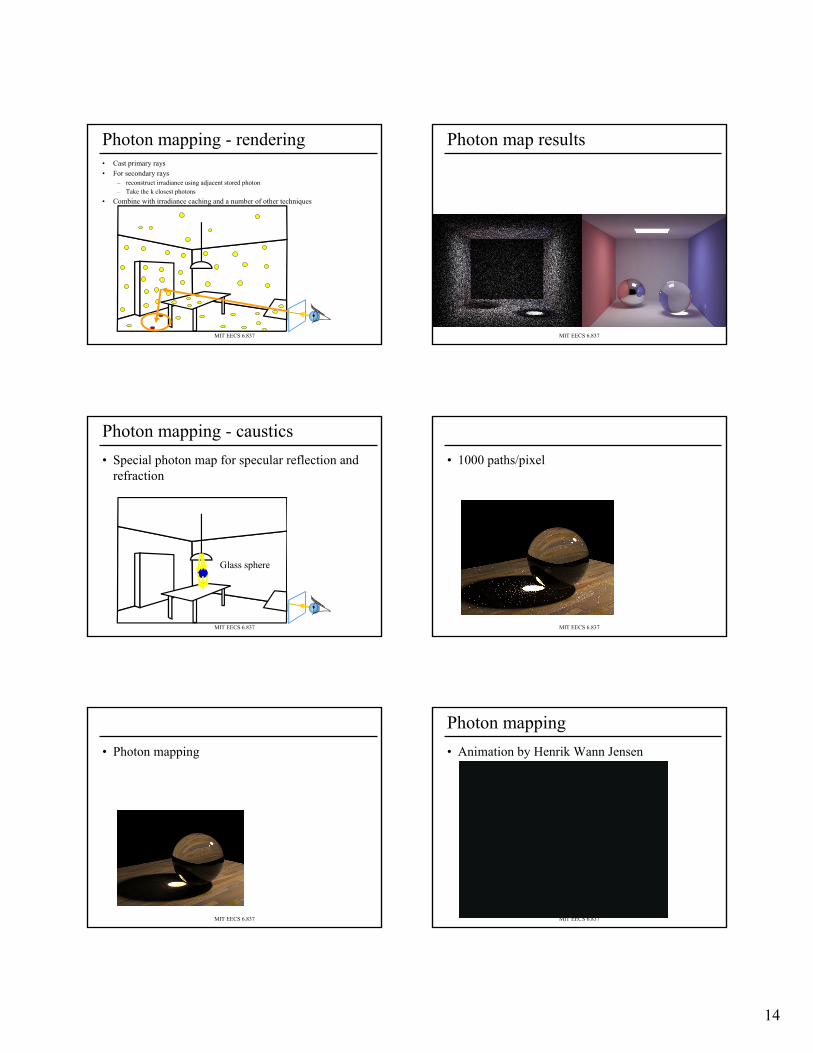
Photon mapping - rendering• Cast primary rays• For secondary rays

– reconstruct irradiance using adjacent stored photon– Take the k closest photons

• Combine with irradiance caching and a number of other techniques

MIT EECS 6.837

Photon map results

MIT EECS 6.837

Photon mapping - caustics• Special photon map for specular reflection and

refraction

Glass sphere

MIT EECS 6.837

• 1000 paths/pixel

MIT EECS 6.837

• Photon mapping

MIT EECS 6.837

Photon mapping• Animation by Henrik Wann Jensen

15

MIT EECS 6.837

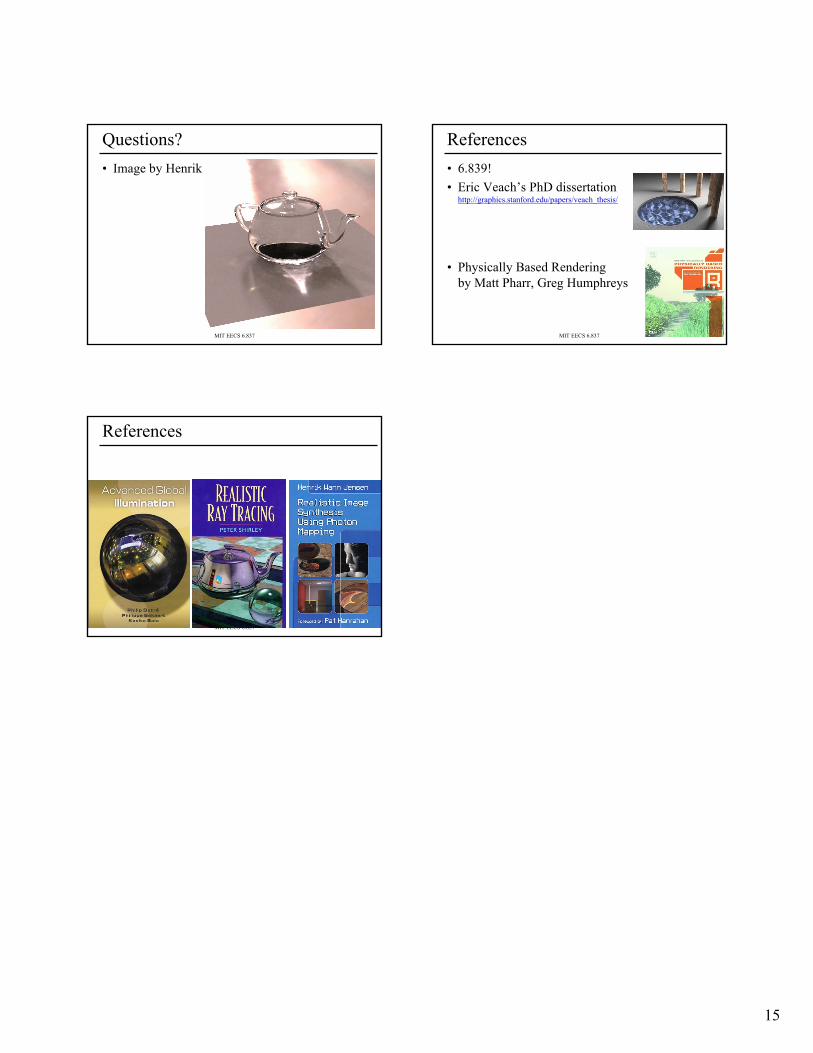
Questions?• Image by Henrik

MIT EECS 6.837

References• 6.839!• Eric Veach’s PhD dissertation

http://graphics.stanford.edu/papers/veach_thesis/

• Physically Based Rendering by Matt Pharr, Greg Humphreys

MIT EECS 6.837

References