Monte Carlo model for analysis of thermal runaway ...

Monte Carlo model for analysis of thermal runaway

electrons in streamer tips in transient luminous

events and streamer zones of lightning leaders

Gregory D. Moss,1 Victor P. Pasko,1 Ningyu Liu,1 and Georgios Veronis2

Received 3 August 2005; revised 9 October 2005; accepted 16 November 2005; published 16 February 2006.

[1] Streamers are thin filamentary plasmas that can initiate spark discharges in relativelyshort (several centimeters) gaps at near ground pressures and are also known to act asthe building blocks of streamer zones of lightning leaders. These streamers at groundpressure, after 1/N scaling with atmospheric air density N, appear to be fully analogous tothose documented using telescopic imagers in transient luminous events (TLEs) termedsprites, which occur in the altitude range 40–90 km in the Earth’s atmosphere abovethunderstorms. It is also believed that the filamentary plasma structures observed in someother types of TLEs, which emanate from the tops of thunderclouds and are termed bluejets and gigantic jets, are directly linked to the processes in streamer zones of lightningleaders. Acceleration, expansion, and branching of streamers are commonly observed for awide range of applied electric fields. Recent analysis of photoionization effects on thepropagation of streamers indicates that very high electric field magnitudes �10 Ek,where Ek is the conventional breakdown threshold field defined by the equality of theionization and dissociative attachment coefficients in air, are generated around the tips ofstreamers at the stage immediately preceding their branching. This paper describes theformulation of a Monte Carlo model, which is capable of describing electron dynamics inair, including the thermal runaway phenomena, under the influence of an external electricfield of an arbitrary strength. Monte Carlo modeling results indicate that the �10 Ek

fields are able to accelerate a fraction of low-energy (several eV) streamer tip electrons toenergies of�2–8 keV. With total potential differences on the order of tens of MVavailablein streamer zones of lightning leaders, it is proposed that during a highly transientnegative corona flash stage of the development of negative stepped leader, electrons withenergies 2–8 keVejected from streamer tips near the leader head can be further acceleratedto energies of hundreds of keV and possibly to several tens of MeV, depending on theparticular magnitude of the leader head potential. It is proposed that these energeticelectrons may be responsible (through the ‘‘bremsstrahlung’’ process) for the generation ofhard X rays observed from ground and satellites preceding lightning discharges or withno association with lightning discharges in cases when the leader process does not culminatein a return stroke. For a lightning leader carrying a current of 100 A, an initial flux of�2–8 keV thermal runaway electrons integrated over the cross-sectional area of the leaderis estimated to be�1018 s�1, with the number of electrons accelerated to relativistic energiesdepending on the particular field magnitude and configuration in the leader streamerzone during the negative corona flash stage of the leader development. These thermalrunaway electrons could provide an alternate source of relativistic seed electrons whichwere previously thought to require galactic cosmic rays. The duration of the negative coronaflash and associated energetic radiation is estimated to be in the range from�1 ms to�1 msdepending mostly on the pressure-dependent size of the leader streamer zone.

Citation: Moss, G., V. P. Pasko, N. Liu, and G. Veronis (2006), Monte Carlo model for analysis of thermal runaway electrons in

streamer tips in transient luminous events and streamer zones of lightning leaders, J. Geophys. Res., 111, A02307,

doi:10.1029/2005JA011350.

1. Introduction

1.1. Streamers in Transient Luminous Events andLightning Leaders

[2] Transient luminous events (TLEs) are large-scaleoptical events in the Earth’s atmosphere that are directly

JOURNAL OF GEOPHYSICAL RESEARCH, VOL. 111, A02307, doi:10.1029/2005JA011350, 2006

1Communications and Space Sciences Laboratory, Pennsylvania StateUniversity, University Park, Pennsylvania, USA.

2Ginzton Laboratory, Stanford University, Stanford, California, USA.

Copyright 2006 by the American Geophysical Union.0148-0227/06/2005JA011350$09.00

A02307 1 of 37

related to electrical activity in underlying thunderstorms.Several types of TLEs are known: relatively slow-movingfountains of blue light, known as ‘‘blue jets,’’ that emanatefrom the top of thunderclouds up to an altitude of 40 km[e.g., Wescott et al., 1995, 2001; Lyons et al., 2003];‘‘sprites’’ that develop at the base of the ionosphere andmove rapidly downward at speeds up to 10,000 km/s [e.g.,Sentman et al., 1995; Lyons, 1996; Stanley et al., 1999];‘‘elves,’’ which are lightning-induced flashes that canspread over 300 km laterally [e.g., Fukunishi et al., 1996;Inan et al., 1997], and recently observed ‘‘gigantic jets,’’which propagate upward, connecting thundercloud topswith the lower ionosphere [e.g., Pasko et al., 2002; Su etal., 2003].[3] Since their discovery, there have been numerous

imaging campaigns in an effort to better understand thephysical phenomena behind these events. Recent imagingcampaigns of sprites [Gerken and Inan, 2005; Marshalland Inan, 2005, and references therein], blue jets [Wescottet al., 2001], and gigantic jets [Pasko et al., 2002] haverevealed a wide variety of fine filamentary structures inthese events, which have been interpreted as streamers.Streamers are narrow filamentary plasmas, which aredriven by highly nonlinear space charge waves [e.g.,Raizer, 1991, p. 327]. Streamers can exhibit both positiveand negative polarities, which is simply defined by thesign of the charge existing in the streamer head. Negativestreamers generally propagate in the same direction as theelectron drift, whereas positive streamers propagate oppos-ing the electron drift. Negative streamers do not requireambient seed electrons to propagate since electron ava-lanches originating from the streamer head propagate inthe same direction as the streamer [e.g., Vitello et al.,1994; Rocco et al., 2002]. Positive streamers, however,must obtain seed electrons from photoionization to sustaintheir propagation [e.g., Dhali and Williams, 1987; Raizer,1991, p. 335].[4] Streamers also serve as precursors to a more com-

plicated leader phenomenon, which involves significantheating and thermal ionization of the ambient gas andrepresents a well known initiation mechanism of break-

down in long gaps [Raizer, 1991, p. 363]. Leaders arethin, highly ionized, highly conductive channels whichgrow along a path prepared by preceding streamers[Raizer, 1991, p. 364]. The head of the highly ionizedand conducting leader channel is normally preceded by astreamer zone looking as a diverging column of diffuseglow and filled with highly branched streamer coronas[e.g., Bazelyan and Raizer, 1998, p. 203, 253]. The leaderprocess is also a well-documented means by which con-ventional lightning develops in thunderstorms [Uman,2001, p. 82], suggesting the presence of numerous stream-ers with every lightning discharge.[5] It has been recently demonstrated that negative

streamers developing in high ambient fields can reach anunstable ‘‘ideal conductivity’’ state with approximatelyequipotential and weakly curved head [Arrayas et al.,2002; Rocco et al., 2002]. This new state exhibits a Lap-lacian instability which can lead to branching of thestreamer [Arrayas et al., 2002; Rocco et al., 2002] andcan be realized over a wide range of applied electric fields[Liu and Pasko, 2004]. Liu and Pasko [2004] also studiedthe effects of photoionization on the dynamics of streamersand determined that the acceleration and expansion ofstreamers results in a reduction of the preionization levelahead of the streamers. In order to compensate for thisreduction in preionization, the magnitude of the electricfield in the streamer tip can reach a value as large as 10Ek atthe stage immediately preceding the branching of thestreamer, where Ek is the conventional breakdown thresh-old field defined by the equality of the ionization anddissociative attachment coefficients in air [e.g., Raizer,1991, p. 135]. Figure 1a shows a negative streamerpropagating at an altitude of 70 km in a 1.5Ek ambientfield as it reaches an unstable state just prior to branching.It can be seen in Figure 1b that an extremely high electricfield exists in the streamer tip prior to branching. Thishigh field �2 kV/m, which spans approximately 1 m (seeFigure 1b), could possibly accelerate low-energy electrons(�several eV) to very high energies �2 keV. As discussedin the next section, the acceleration of electrons in thesehighly overvolted streamer tips could contribute to the

Figure 1. (a) A cross-sectional view of the distribution of the electron number density for a modelnegative streamer at 70 km altitude immediately preceding branching and (b) the electric field in thestreamer tip immediately preceding branching.

A02307 MOSS ET AL.: MONTE CARLO MODEL OF THERMAL RUNAWAY ELECTRONS

2 of 37

A02307

formation of high-energy electron fluxes needed to explainthe recently observed X-ray [Moore et al., 2001; Dwyer etal., 2003, 2004a, 2004b, 2005] and gamma ray [Fishmanet al., 1994; Smith et al., 2005] bursts associated withthunderstorm activity.[6] The model streamer shown in Figure 1 was obtained

using the numerical model described by Liu and Pasko[2004] and assuming that no preionization is producedahead of the streamer due to photoionization effects. Theseconditions are expected to be close to those realized beforestreamer branching when the photoionization rangebecomes shorter than the radius of the expanding streamer(see sections 4.1 and 4.4 in the work of Liu and Pasko[2004] for additional details).

1.2. Runaway Electrons and Energetic Radiation

[7] Runaway electrons were discussed by Gurevich[1961] and were defined by Kunhardt et al. [1986], whostated ‘‘an electron is runaway if it does not circulatethrough all energy states available to it at a given E/N,but on average moves toward high-energy states.’’ Therunaway phenomenon is a result of decreasing probabilityof electron interactions with atomic particles for electronenergies in the range from �100 eV to �1 MeV [Gurevich,1961]. This phenomenon can best be understood by con-sidering the dynamic friction force of electrons in air as afunction of electron energy (see Figure 2):

FD eð Þ ¼Xj

Nj sj eð Þ d�j; ð1Þ

where the summation is performed over all inelasticcollision processes of a given gas with partial density Nj

of N2, O2, or Ar in air (in m�3) corresponding to aparticular collision process defined by the cross section sjand energy loss d�j. In plotting FD(e) (Figure 2), electron-neutral collision cross sections provided by Phelps (http://jilawww.colorado.edu/www/research/colldata.html) andmass radiative and collision stopping powers [InternationalCommission on Radiation Units and Measurements, 1984]were used. Electron energy losses due to nonzero energiesof secondary electrons emerging from ionizing collisionswith N2, O2, and Ar were accounted for using thedifferential ionization cross sections provided by Opal etal. [1971] (see section 2.3).[8] Electrons under the influence of an electric field E

experience a force FE = �qeE and an acceleration dvdt

according to the Lorentz force law and Newton’s secondlaw, respectively, where qe is the absolute value of electroncharge. As the electron accelerates through a gas it experi-ences collisions with the neutral gas molecules and atoms,which give rise to the dynamic friction force FD opposingthe force applied by the electric field FE. It can be seen inFigure 2 that the friction force FD varies considerably withelectron energy. For example, a maximum exists in FD at�100 eV which is �103 the value of FD at 1 eV. Physicallyspeaking, a 100 eV electron experiences many more colli-sions and loses much more energy per unit length of itstrajectory than does a 1 eV electron.[9] FD has units of eV/cm and can be directly compared

to the applied electric field to provide an intuitively simple

Figure 2. The dynamic friction force of electrons in air at ground pressure is plotted as a function ofelectron energy. A solid line corresponds to a case when a total of 43 inelastic processes were accountedfor corresponding to an air mixture of 78.11% N2, 20.91% O2 and .98% Ar gases using a set of crosssections compiled by A. V. Phelps (http://jilawww.colorado.edu/www/research/colldata.html), whichexcludes dissociation processes. A dotted line corresponds to a case which includes energy losses due todissociation of N2 and O2 molecules.


3 of 37

A02307

insight into the expected motion of electrons at variousenergies. Figure 2 lists electric fields required to initiatevarious types of electrical breakdown in air (more detailsand related references may be found in the work of Pasko[2006]) and displays the respective force FE, in units ofeV/cm, they apply to electrons in relationship to thefriction force FD. Of particular interest to the theory ofrunaway electrons is the maximum in FD at �100 eV andthe corresponding electric field which is known as thethermal [Gurevich, 1961] runaway threshold (Ec). Elec-trons with energies �100 eV moving through air willexperience many collisions with neutral particles, whichgive rise to a high value of FD. If an electric field E < Ec

is applied to the electrons, the force FE will be less thanthe force FD the electrons will experience from collisions;therefore the electrons will be maintained at energies<100 eV. However, if an electric field E > Ec is applied to theelectrons, it can be seen from Figure 2 that FE > FD. Theelectrons will gain more energy from the electric field thanthey will lose to collisions. It then becomes possible forsome of the electrons to be energized to energies >100 eV.Owing to the reduced probability of collisions of electronswith energies >100 eV, the electrons will continue toaccelerate to very high runaway energies as long as theelectric field is present. Electric fields above Ec are difficultto produce and maintain since the electron runaway is alsoaccompanied by an avalanche multiplication of electronsand strong increase in plasma conductivity, which tends toreduce the applied field. Electric fields �10Ek around tips ofpropagating streamers (Figure 1) are one of the uniquenaturally occurring circumstances when such high fieldscan be dynamically produced and sustained for relativelyextended periods of time.[10] Also of interest is the minimum in FD which occurs

at �1 MeV. This is known as the relativistic [Gurevich etal., 1992; Roussel-Dupre et al., 1994] runaway threshold

(Et) and is the basis of the Relativistic Runaway ElectronAvalanche (RREA) model proposed by Gurevich et al.[1992]. At electron energies around 1 MeV the probabilityof collisions with neutrals is greatly decreased and anyelectron with an initial energy in this region (e.g., cosmicray secondaries with energies 0.1–1 MeV [e.g., Roussel-Dupre et al., 1994; Gurevich and Zybin, 2005]) will runaway when an electric field >Et is applied. According to theRREA model, as few as one energetic electron (�1 MeV)can trigger an avalanche of runaway electrons, via ioniza-tion of air molecules and atoms, which will continue togrow as long as an electric field E > Et is present.[11] Additionally, at lower electric fields comparable to

the conventional breakdown field Ek, electrons are expectedto be held to energies <20 eV by collisional losses since FD >FE for energies >20 eV. At even lower field values (i.e.,fractions of Ek) electrons will be trapped by the localmaximum in FD around 1–2 eV resulting from strong energylosses due to excitation of vibrational degrees of freedomof nitrogen and oxygen molecules. The discrete structureobserved at energies <1 eV also arises from the excitation ofrotational degrees of freedom of nitrogen molecules and theexcitation of rotational and vibrational degrees of freedom ofoxygen molecules.[12] The production of runaway electrons in the Earth’s

atmosphere has recently been linked to X-ray and gammaray bursts observed during lightning discharges [Moore etal., 2001; Dwyer et al., 2003, 2004a, 2004b, 2005]. Inaddition to these ground-based measurements, intense gam-ma ray flashes originating from the Earth’s atmosphereabove thunderstorms have also been observed by theCompton Gamma Ray Observatory (CGRO) and theReuven Ramaty High Energy Solar Spectroscopic Imager(RHESSI) satellites [Fishman et al., 1994; Smith et al.,2005]. While these observations strongly support the exis-tence of extremely high-energy electrons during thunder-storm activity, the exact mechanism producing themremains under debate [e.g., Dwyer, 2005a]. Gurevich[1961] showed that in the presence of extremely strongelectric fields, a large number of low-energy electrons canbe directly accelerated over the peak of the friction forceFD and become thermal runaway electrons. This is arelatively straightforward approach to runaway develop-ment and is readily accepted. However, since the electricfield strengths necessary to achieve thermal runaway (E �10Ek) and even conventional (E � Ek) breakdown are notcommonly observed on large spatial scales in thunder-clouds [Marshall et al., 1995, 2005], many scientistsabandoned thermal runaway breakdown as a source ofrunaway electrons during thunderstorms and adopted thenewer theory of RREA. One of the goals of the presentpaper is to demonstrate that streamers may represent arealistic source of thermal runaway electrons and discusscircumstances when these electrons can be accelerated tovery high (>1 MeV) energies, thus providing an alternatesource of seed electrons to the RREA model previouslythought to require galactic cosmic rays.

1.3. Purpose of This Paper

[13] This paper presents the formulation of a Monte Carlomodel, which is capable of describing electron dynamics inair including the electron thermal runaway phenomena

Table 1. Molecular Nitrogen Collision Processes

CollisionProcess Reaction

ThresholdEnergy, eV

N2 elastic e + N2 ! e + N2 -N2 rotational e + N2 ! e + N2(rot) 0.02N2 vibrational e + N2 ! e + N2(v = 1) 0.29

e + N2 ! e + N2(v = 1) 0.291e + N2 ! e + N2(v = 2) 0.59e + N2 ! e + N2(v = 3) 0.88e + N2 ! e + N2(v = 4) 1.17e + N2 ! e + N2(v = 5) 1.47e + N2 ! e + N2(v = 6) 1.76e + N2 ! e + N2(v = 7) 2.06e + N2 ! e + N2(v = 8) 2.35

N2 electronic e + N2 ! e + N2(A3Su

+, v = 1–4) 6.17e + N2 ! e + N2(A

3Su+, v = 5–9) 7.00

e + N2 ! e + N2(B3�g) 7.35

e + N2 ! e + N2(W3Du) 7.36

e + N2 ! e + N2(A3Su

+, v = 10+) 7.80e + N2 ! e + N2(B

03Su�) 8.16

e + N2 ! e + N2(a01Su

�) 8.40e + N2 ! e + N2(a

1�g) 8.55e + N2 ! e + N2(w

1Du) 8.89e + N2 ! e + N2(C

3�u) 11.03e + N2 ! e + N2(E

3Sg+) 11.88

e + N2 ! e + N2(a001Sg

+) 12.25N2 sum ofsinglet states

e + N2 ! e + N*2 13.00

N2 ionization e + N2 ! e + e + N2+(X2Sg

+ + A2�u) 15.60


4 of 37

A02307

under influence of an external electric field of arbitrarystrength. The model is similar in technical details to themodel previously developed for N2 by Tzeng and Kunhardt[1986] and incorporates the following features: (1) the‘‘null’’ collision method to determine time between colli-sions [Lin and Bardsley, 1977]; (2) the remapping of theelectron assembly to improve statistics for the high-energytail of the electron distribution [Kunhardt and Tzeng,1986b]; (3) the differential ionization [Opal et al., 1971]and scattering cross sections for realistic description ofenergy spectrum of secondary electrons and the forwardscattering properties of electrons at high energies. Resultsfor zero-dimensional modeling of the electron distributionunder the influence of a uniform electric field are firstpresented and compared with existing data. At high electricfields the model is validated by comparisons with studiesconducted for N2 by Tzeng and Kunhardt [1986] and morerecently by Bakhov et al. [2000]. At low electric fields,model results are compared to available data from swarmexperiments in air [Davies, 1983], numerical solutions ofthe Boltzmann equation based on the two-term sphericalharmonic expansion of the electron distribution function[Morgan and Penetrante, 1990], and analytical modelsproposed by Aleksandrov et al. [1995] and Morrow andLowke [1997]. The new Monte Carlo model is then appliedto a one-dimensional case corresponding to a negativestreamer tip immediately preceding branching. The modelresults demonstrate that the electric fields in streamer tips arestrong enough to accelerate low-energy electrons to severalkeV, initiating thermal runaway in relatively low ambientfields. Streamers have been documented in transient lumi-nous events above thunderclouds and in streamer zones ofconventional lightning leaders and may provide a robustsource of runaway electrons contributing to the productionof recently observed X-ray and gamma ray bursts.

2. Model Formulation

2.1. Collision and Scattering Cross Sections

[14] Essential to both the numerical Boltzmann equationsolution and the Monte Carlo method describing behavior

of electrons in weakly ionized air is the knowledge ofelectron-atom and electron-molecule collision cross sectionsfor each gas species. Generally, atoms and molecules in aweakly ionized gas are assumed to be heavy and remainstationary; therefore the collision cross section becomessimply a function of the electron energy.[15] For the Monte Carlo model presented in this paper

several different cross section sets were used to determinean electron’s motion through air. A total of 46 collisionprocesses were considered corresponding to the N2, O2, andAr gases included in the air mixture (see Tables 1, 2, and 3).Each gas has an associated elastic cross section accountingfor elastic collisions and a set of inelastic cross sections (24for N2, 17 for O2 and 2 for Ar) accounting for each inelasticcollision process (i.e., rotational, vibrational, and electronicexcitations, ionization, and attachment).[16] The 43 inelastic cross sections sinel were obtained

directly from the compilation of A.V. Phelps (http://jilawww.colorado.edu/www/research/colldata.html). Theelastic collision cross section sel for each gas was thendetermined by subtracting the summation of inelastic crosssections from the total collision cross sections

sel;s ¼ st;s �Xj

sinel;j;s; ð2Þ

where s represents a specific gas species and the summationis performed over all inelastic collision processes with jrepresenting the jth process. The total collision cross sec-tions were obtained from experimental data reported inliterature as summarized in Table 4.[17] The calculated elastic cross sections and the inelastic

cross sections are the fundamental quantities used to deter-mine an electron’s interaction with the gas medium. Fromthese collision cross sections the mean free path, mean timebetween collisions, and collision frequency of an electron inthe gas medium can be calculated as

l ¼ 1

Nsð3Þ

t ¼ lv

ð4Þ

n � t�1 ¼ Nsv; ð5Þ

respectively, where N is the gas density, s is the collisioncross section, and v is the electron’s velocity.[18] In addition to the collision cross sections mentioned

above, the differential scattering cross section dsdW for each

gas must be known to determine the angular scattering ofelectrons after a collision. Experimental values for theelastic differential scattering cross sections were obtained

Table 2. Molecular Oxygen Collision Processes

CollisionProcess Reaction

ThresholdEnergy, eV

O2 elastic e + O2 ! e + O2 -O2 rotational e + O2 ! e + O2(rot) 0.02O2 vibrational e + O2 ! e + O2(v = 1, e < 4 eV) 0.19

e + O2 ! e + O2(v = 2, e < 4 eV) 0.38e + O2 ! e + O2(v = 3) 0.57e + O2 ! e + O2(v = 4) 0.75

e + O2 ! e + O2(v = 1, e > 4 eV) 0.19e + O2 ! e + O2(v = 2, e > 4 eV) 0.38

O2 electronic e + O2 ! e + O2(a1Dg) 0.977

e + O2 ! e + O2(b1Sg

+) 1.627e + O2 ! e + O2(c

1Su�) 4.50

e + O2 ! e + O(3P) + O(3P) 6.00e + O2 ! e + O(3P) + O(1D) 8.40e + O2 ! e + O(1D) + O(1D) 10.00e + O2 ! e + O(3P) + O(3S0) 14.70

O2 ionization e + O2 ! e + e +O2+(X2�g) 12.06

O2 three-bodyattachment

e + O2 + A ! O2� + A -

O2 two-bodyattachment

e + O2 ! O� + O -

Table 3. Argon Collision Processes

Collision Process Reaction Threshold Energy, eV

Ar elastic e + Ar ! e + Ar -Ar electronic e + Ar ! e + Ar* 11.50Ar ionization e + Ar ! e + e + Ar+ 15.80


5 of 37

A02307

from literature (see Table 5). The angular scattering ofelectrons in inelastic collisions was determined using theelastic differential cross sections listed in Table 5. Thisassumption is reasonable for scattering of electrons on themolecules with excitation of singlet states (predominantlyforward) but may introduce error for the scattering involv-ing excitation of the triplet states, which possess astronger backscatter component [Tzeng and Kunhardt,1986]. Figure 3 shows the elastic differential scatteringcross section, for low-energy scattering obtained fromsources listed in Table 5 for N2, O2, and Ar. It can be seenfrom Figure 3 that at electron energies <20 eV the angularscattering of electrons is generally isotropic but quicklybecomes forward for electron energies >20 eV. Electronswith energies 0 eV were assumed to demonstrate isotropicscattering and the differential cross section values from 0 to5 eV for N2, 0 to 2 eV for O2, and 0 to 3 eV for Ar weredetermined using linear interpolation.[19] For use in the Monte Carlo calculations, differential

cross section tables for each gas were generated using linearinterpolation of the data from sources listed in Table 5. Thetables are then related to a uniform random number Rc from0 and 1 as

Rc ¼

Z c

0

2pdsdW

sinc dcZ p

0

2pdsdW

sinc dc; ð6Þ

where c is the scattering angle of an electron. The scatter-ing angle c can then easily be found by performing a tablelookup using a random number Rc and the electron energye. Angular scattering of electrons with energies in the range0–500 eV experiencing collisions with N2, and in the rangeof 0–1000 eV colliding with O2 and Ar is determined usinglookup tables derived from published experimental datafrom sources given in Table 5.

2.2. High-Energy Electron Scattering

[20] For collisions involving electrons with energiesgreater than those tabulated from the experimental data(>500 eV for N2 collisions, >1000 eV for O2 and Arcollisions), differential scattering cross sections are calcu-lated using several different approximations. It is theshortage of cross section data at high electron energiesthat remains the largest source of error in Monte Carlo

simulations and there is no commonly accepted approxi-mation which is universally used.[21] For low-energy electrons, the dominant process is

relatively short-range polarization scattering [Liebermanand Lichtenberg, 1994, p. 60]. However, the mean collisiontime (equation (4)) of high-energy electrons is small, notallowing atoms and molecules adequate time to polarize.Therefore high-energy electron scattering from neutralparticles (i.e., electron-atom and electron-molecule colli-sions) resembles Coulomb-like collisions between chargedparticles (i.e., electron-electron, electron-ion, and ion-ioncollisions) [Lieberman and Lichtenberg, 1994, p. 60].[22] The differential cross section for Coulomb-like col-

lisions can be analytically derived as

dsdW

¼ b0

4 sin2 c=2ð Þ

� �2ð7Þ

b0 ¼q1 q2

4p e0 e; ð8Þ

where q1 and q2 are charges of projectile and targetparticles, e0 is the permittivity of free space, e is the center-of-mass energy, and b0 is known as the classical distance ofclosest approach. Equation (7) is the well known Rutherfordcross section for Coulomb scattering [Lieberman andLichtenberg, 1994, p. 57]. In a general case, however, theRutherford cross section cannot be directly used in MonteCarlo simulations because of the singularity as c ! 0. Forthis reason, a wide number of approximations based onscreened Coulomb scattering have been implemented todetermine the angular scattering of high-energy electrons inMonte Carlo and Boltzmann equation solutions.[23] A. V. Phelps (http://jilawww.colorado.edu/www/re-

search/colldata.html) presents an analytical differential scat-tering cross section approximation for elastic electronscattering from N2 based on a screened-Coulomb typescattering

dsdW

¼ 1

1� 1� 2b eð Þð Þ cosc½ �2ð9Þ

b eð Þ ¼ :6

1þffiffiffiffiffiffiffiffiffiffie=50

pþ e=20ð Þ1:01

h i0:99 ; ð10Þ

where here and in subsequent equations e is in units ofeV and b(e) is an algebraic screening parameter derived tofit experimental angular distributions from Phelps and

Table 4. Total Collision Cross Section Data Sources

Gas Energy Range, eV Literature Source

N2 0–0.4 Phelps and Pitchford [1985]0.4–250 Szmytkowski et al. [1996]250–600 Blaauw et al. [1980]600–5000 Garcia et al. [1988]

5000–10,000 Phelps and Pitchford [1985]O2 0–0.4 Lawton and Phelps [1978]

0.4–250 Szmytkowski et al. [1996]250–500 Dababneh et al. [1988]500–5000 Jain and Baluja [1992]

5000–10,000 extrapolated from Jain and Baluja [1992]Ar 0–0.4 Yamabe et al. [1983]

0.5–220 Szmytkowski et al. [1996]300–5000 Karwasz et al. [2002]

5000–10,000 extrapolated from Karwasz et al. [2002]

Table 5. Differential Scattering Cross Section Data Sources

Gas Energy Range, eV Literature Source

N2 5–90 Shyn et al. [1972]100–500 Kambara and Kuchitsu [1972]

O2 2–200 Shyn and Sharp [1982]300–1000 Iga et al. [1987]

Ar 3–100 Srivastava et al. [1981]150–400 Williams and Willis [1975]200–500 DuBois and Rudd [1976]800–1000 Iga et al. [1987]


6 of 37

A02307

Pitchford [1985]. Substituting equation (9) into equation (6)and solving for the scattering angle c results in

c ¼ arccos1� b eð Þ � Rc

1� b eð Þ � Rc þ 2 b eð ÞRc

� �; ð11Þ

where Rc is a uniform random number between 0 and 1.[24] Surendra et al. [1990] proposed an analytical

expression based on screened Coulomb scattering from Ar

dsdW

¼ e4p 1þ e sin2 c=2ð Þ

ln 1þ eð Þ

ð12Þ

such that the electron-neutral scattering at low energies ismainly isotropic and becomes increasingly anisotropic asthe electron energy increases. Substituting equation (12)into equation (6) and solving for the scattering angle cresults in

c ¼ arccos2þ e� 2 1þ eð ÞRc

e

" #: ð13Þ

[25] In his study of an electron avalanche developmentin neon, Shveigert [1990] used the differential scatteringcross section for the scattering of fast electrons byshielded Coulomb potential of a nucleus as publishedby Kol’chuzhkin and Uchaikin [1978]:

dsdW

¼ 1

4

Z Z þ 1ð Þe2

q4e1

1� coscþ 2hð Þ2ð14Þ

h ¼ 20 eþ 96ð Þe2

; ð15Þ

where Z is the number of protons in the atom’s nucleus andh is the shielding parameter formulated to fit the calcula-tions of Thomas [1969] at e = 100 eV. Scattering anglesfrom this approximation are tabulated numerically usingequation (6).[26] A modified Rutherford cross section was also intro-

duced for use in this paper of the form

dsdW

¼ e=e14p arctan e=e1ð Þ

1

1þ e2=e21 �

sin4 c=2ð Þ; ð16Þ

where e1 is a shape parameter which is set to e1 = 4 eV tomatch experimental data of Kambara and Kuchitsu [1972]for electron scattering from N2 at 500 eV. Substitutingequation (16) into equation (6) and solving for the scatteringangle c results in

c ¼ 2 arcsin

ffiffiffiffiffiffiffiffiffiffiffiffiffiffiffiffiffiffiffiffiffiffiffiffiffiffiffiffiffiffiffiffiffiffiffiffiffiffiffiffiffiffiffiffiffiffiffiffiffiffiffiffiffie1=eð Þ tan Rc arctan e=e1ð Þ

�q� �: ð17Þ

[27] The differential cross section used to approximatehigh-energy electron scattering can greatly impact thegeneration of runaway electrons and will be discussedfurther in sections 3.3, 4.1, and 4.2. Figure 4 shows thedifferential cross sections described by equations (9), (12),(14), and (16).[28] It should be noted that while Figures 4a through 4d

are plotted for the energy range 0–1000 eV, the crosssections are only used in the model for collisions with N2

where e > 500 eV and collisions with O2 and Ar where e >1000 eV. Figure 5a shows a comparison of equations (9),(12), (14), and (16) with experimental data of Kambaraand Kuchitsu [1972] for electron collisions with N2 at e =500 eV and Figure 5b shows a similar comparison withexperimental data of Iga et al. [1987] for electron colli-sions with O2 at e = 1000 eV. Upon first examination ofFigures 4 and 5, the differences between the differentialcross sections may appear to be small. However, theforward scattering properties of high-energy electrons arevital in the development of electron runaway and thesesmall variations can drastically hinder or facilitate therunaway process (sections 3.3, 4.1, and 4.2).

2.3. Differential Ionization Cross Section

[29] The behavior of the phase-space distribution ofelectrons is strongly influenced by ionization and the angleand energy of each of the two electrons emerging from thecollision [Tzeng and Kunhardt, 1986]. Tzeng and Kunhardt[1986] placed special emphasis on the energy partitioningused in ionizing collisions and presented results for fourseparate cases:[30] In case 1 the secondary electron is assigned zero

energy, leaving the primary electron with the differencebetween initial energy and the ionization energy. In case 2the energy of the secondary is determined from the differ-ential cross section for ionization determined from experi-ments by Opal et al. [1971]. In case 3 the fraction of half theavailable energy given to the secondary is a random variable

Figure 3. Elastic differential scattering cross section of N2, O2, and Ar gases for electron energiesranging from 0 to 100 eV.


7 of 37

A02307

Figure 4. Differential scattering cross section of Phelps (a) (http://jilawww.colorado.edu/www/research/colldata.html) calculated using equation (9) of Surendra et al. [1990] (b) based on equation (12) ofKolchuzhkin and Uchaikin [1978] (c) described by equation (14), and (d) as calculated usingequation (16).

Figure 5. The differential scattering cross section for (a) 500 eV and (b) 1000 eV electrons calculatedfrom equations (9), (12), (14), and (16) compared with experimental data of Kambara and Kuchitsu[1972] and Iga et al. [1987], respectively.


8 of 37

A02307

uniformly distributed in the interval [0,1]. In case 4 theprimary and secondary electrons equally share the availableenergy.[31] The differences in the energy distribution functions

for each of these cases are significant, especially at highelectron energies. The variations can best be explained byconsidering the energy of the incident electron after anionizing collision

e0p ¼ ep � eiz � es; ð18Þ

where ep is the energy of the incident electron before thecollision, es is the energy of the secondary electrongenerated by the collision, and eiz is the ionization potential.For cases 3 and 4 the high-energy incident electronsparticipating in the ionizing collisions lose a large fractionof their energy to the secondary electron (es is large), thusseverely reducing the number of electrons which canaccelerate to runaway energies. In contrast, incidentelectrons in case 1 lose only energy equal to the ionizationpotential, eiz, (es = 0), thus contributing to an overpopulationof electrons existing at very low energies due to the low-energy secondaries as well as an overpopulation of runawayenergy electrons due to high-energy incident electronslosing only a small fraction of their energy to ionizingcollisions. Among the cases presented, case 2, which makesuse of the secondary energy distribution suggested by Opalet al. [1971], is the most realistic [Tzeng and Kunhardt,1986] and is used for all simulations presented in this paper.[32] Opal et al. [1971] measured a quantity proportional

to the doubly differential cross section s(ep, es, c). Inte-grating this cross section over the angle c, results in

s ep; es �

¼Z p

0

s ep; es;c �

2p sinc dc: ð19Þ

Assuming the ion to be massive and at rest, the kineticenergy imparted to the ion in the collision is negligible andthe energies of the two departing electrons must sum to ep �eiz and be symmetrical about (ep � eiz)/2 [Opal et al., 1971].The total ionization cross section can then be given by

si ep �

¼Z ep�eizð Þ=2

0

s ep; es �

des: ð20Þ

From results of their experiments, Opal et al. [1971]determined the differential ionization cross section to be

s ep; es �

¼si ep �

e arctan ep � eiz �

=2e 1

1þ es=eð Þ2; ð21Þ

where e is a shape parameter adjusted to fit the ejectedelectron spectrum. Values of e determined by Opal et al.[1971] are listed in Table 6 for N2, O2, and Ar gases.

[33] The differential ionization cross section of Opal et al.[1971] can be used to determine the energy es of thesecondary electron. Similarly to the determination of thescattering angle from the differential scattering cross sectionfrom equation (6), es can be related to a uniform randomnumber Res by performing the integration

Res ¼

Z es

0

s ep; es �

desZ ep�eizð Þ=2

0

s ep; es �

des

: ð22Þ

Observing that the denominator of equation (22) is the totalionization cross section si(ep) and substituting the differ-ential ionization cross section of Opal et al. [1971] (21),equation (22) can be rewritten as

Res ¼1

e arctan ep � eiz �

=2e Z es

0

1

1þ es=eð Þ2des

¼ arctan es=eð Þarctan ep � eiz

�=2e

: ð23Þ

Solving equation (23) for the secondary electron energy esresults in

es ¼ e tan Res arctanep � eiz

2e

� �h i: ð24Þ

[34] Also, as mentioned in section 1.2, the differentialionization cross section of Opal et al. [1971] was used inthe determination of the dynamic friction force in air (seeFigure 2). Using the differential cross section defined byequation (21), the average energy of a secondary electronemerging from an ionizing collision can be found as

hes ep �

i ¼ 1

si ep � Z ep�eiz

2

0

es s ep; es �

des

¼ e

2 arctanep � eiz

2e

� � ln 1þep � eiz �2

4e2

" #: ð25Þ

After obtaining the average secondary energy hes(ep)i, thefriction force of ionizing collisions can be calculated as

FI eð Þ ¼ Njsj eð Þ eiz;j þ hes;j eð Þi

; ð26Þ

where the index j accounts for differences in the ionizationpotential and the average secondary energy correspondingto different target species with density Nj.

2.4. Null Collision Method

[35] The Monte Carlo method works by individuallytracking each electron in an assembly through a series oftime steps until an equilibrium state is attained (e.g.,electron mean energy remains constant). In a given timestep, Dt, the electron may or may not experience a collisionwith the probability of a collision being [Dincer andGovinda Raju, 1983]

P ¼ 1� e�Dtt ; ð27Þ

Table 6. Ionization Energies eiz and Ejected Electron Spectrum

Shape Parameter e in eV [Opal et al., 1971]

Gas eiz e

N2 15.6 13.0O2 12.2 17.4Ar 15.7 10.0


9 of 37

A02307

where t is the mean time between collisions of an electrondefined by equation (4). We note that the mean collisiontime in equation (4) depends on the electron’s velocity.Therefore for a large number of electrons included in asimulation, there will be an equally large number of distincttime steps between collisions. The computation required tosupport each electron possessing its own mean collisiontime is a daunting task and can be overcome by adopting anull collision technique [Lin and Bardsley, 1977], whichallows a constant mean collision time to be defined for allelectrons in the system. The null collision approach firstdefines the total collision frequency as the sum of all elasticand inelastic collision frequencies

nt eð Þ ¼Xnj¼1

nj eð Þ ¼Xnj¼1

Njsj eð Þv eð Þ; ð28Þ

where

v eð Þ ¼ffiffiffiffiffiffiffiffiffiffiffi2 qe em

r; ð29Þ

m is the mass of an electron, and Nj represents a partialdensity of target molecules or atoms corresponding to aparticular collision process defined by the cross section sj.Having plotted nt(e) versus electron energy (as schemati-cally shown at the top of Figure 6), the maximum collisionfrequency nmax can be found

nmax ¼ max nt eð Þ½ �: ð30Þ

The constant mean collision time tc can then be calculatedby substituting nmax into equation (5)

tc ¼1

nmax

: ð31Þ

A constant time step Dt can then be defined as

Dt ¼ dnmax

¼ dtc; ð32Þ

where d is an arbitrary number much less than 1. In allcalculations presented in this paper, d is assumed to be equalto 0.1 (see Figure 6).[36] Now, having obtained a constant time step to be

used throughout the simulation, the null collision tech-nique can be viewed as a three step procedure usingthree uniform random numbers between 0 and 1 todetermine if an electron experiences a collision in atime step, and if so, what type of collision it was. Anoutline of the null collision method is provided inFigure 6.[37] 1. Substituting tc and Dt into equation (27) results in

a constant probability of a collision in a time step

Pcoll ¼ 1� e�dtctc ¼ 1� e�d ’ d ¼ 0:1: ð33Þ

Therefore if a uniform random number R1 from 0 to 1 is lessthan 0.1 for a given electron, the electron is said to haveexperienced a collision in the time step.[38] 2. Having determined that an electron experienced a

collision in step 1, we must now determine whether thecollision is a null or real collision. The energy independentmaximum collision frequency nmax defined by equation(30) can be represented as the sum of the energy dependentnull nnull(e) and real nt(e) collision frequencies (see top ofFigure 6)

nmax ¼ nt eð Þ þ nnull eð Þ: ð34Þ

The probability of a real collision, Preal, can then be definedas

Preal eð Þ ¼ nt eð Þnmax

ð35Þ

and is a function of the electron energy e. For eachelectron which was determined to have experienced acollision in step 1, a second random number R2 with auniform distribution between 0 and 1 is generated andcompared with the probability Preal corresponding to theelectron’s energy. If R2 � Preal the collision is consideredto be real, otherwise (R2 > Preal) the collision is consideredto be null and has no effect on the electron’s properties(see Figure 6).[39] 3. If the collision was determined to be real in step 2,

then the next step is to determine what type of collision (i.e.,momentum transfer, excitation, ionization) occurred. At agiven electron energy ej, there is a collection of individualcollision frequencies nj(e), which sum to equal the totalcollision frequency nt(e) as shown by equation (28). Theprobability of each collision process can then be calculatedas

Pj ¼nj eð Þnt eð Þ ð36Þ

Figure 6. Schematic summary of the null collision methodused in the Monte Carlo simulation.


10 of 37

A02307

at a given electron energy e such that

Xnj¼1

Pj ¼ 1: ð37Þ

Each collision process can then be assigned a range ofnumbers existing between 0 and 1 by performing acumulative summation of the individual probabilities Pj

such that Range 1 = 0 to P1, Range 2 = P1 to P1 + P2, Range3 = P1 + P2 to P1 + P2 + P3, etc. A third uniform randomnumber R3 between 0 and 1 can then be generated andwhichever process’s range it falls within is determined to bethe collision process which occurred (see Figure 6).[40] To better illustrate the procedures of step 2 and step 3,

consider a simple case of only argon gas. The collisionfrequencies of argon are shown in Figure 7a. Normalizingthe collision frequencies according to equation (35) resultsin values between 0 and 1 as shown in Figure 7b. FromFigure 7b it can be seen that for a 100 eV electron, thetotal normalized collision frequency is 0.0825 + 0.3092 +0.4709 = 0.8626. A real collision is said to occur ifrandom number R2 is such that 0 < R2 < 0.8626 and anull collision occurs if R2 > 0.8626. If it is determined thata real collision has occurred, then the collision processesmust be normalized by the value of the total collisionfrequency at 100 eV of 0.8626 as shown in Figure 7c.Now random number R3 will be generated to determinewhich type of collision occurred. If 0 < R3 < 0.5459, thecollision is said to be elastic. If 0.5459 < R3 < 0.6415(where 0.5459 + 0.0956 = 0.6415), the collision is said tobe excitation. Finally, if 0.6415 < R3 < 1 (where 0.6415 +0.3585 = 1), the collision is said to be ionization. After thetype of collision is determined, the electron’s properties(i.e., energy, velocity, direction) are modified accordinglyas described in section 2.5 below.[41] After simulating each electron’s interactions

through a time step as described in steps 1, 2, and 3,the electron velocities are updated to reflect accelerationdue to the applied electric field and diagnostic data issaved. If a specified number of electrons has beenreached due to ionization processes, a particle remappingscheme (section 2.6) is applied to avoid undesirably longcomputation times. The procedure above is then repeateduntil an equilibrium state is reached or until a point intime, which is defined by an investigator.

2.5. Energy Loss and Scattering of Electrons

[42] There are four types of collision processes consid-ered in this paper: elastic, excitation, ionization, and attach-ment. When one of these collision processes occur in aMonte Carlo simulation (see section 2.4), the colliding

Figure 7. (a) Ar total, elastic, ionization, and excitation collision frequencies as a function of electronenergy, (b) the normalized collision frequencies to determine the occurrence of a null or real collision,(c) and normalized frequencies by the total collision frequency at 100 eV to determine the type ofcollision (see text for details).

Figure 8. Summary of electron-atom/molecule collisionsin air.


11 of 37

A02307

electron’s energy and trajectory following the collision mustbe determined. A summary of these collisions is shown inFigure 8.[43] First, consider an electron characterized by its per-

pendicular v? and parallel vk velocity components withrespect to the applied electric field and angles qc and fc asshown in Figure 9a, where

vj j ¼ffiffiffiffiffiffiffiffiffiffiffiffiffiffiffiv2k þ v2?

qð38Þ

v? ¼ vj j sin qc ð39Þ

vk ¼ vj j cos qc: ð40Þ

Since only electron collisions with massive, stationaryneutral atoms and molecules are considered, scatteringevents can be treated in center-of-mass coordinates[Lieberman and Lichtenberg, 1994, p. 51]. For simplicity,the initial angle fc is assumed to be zero and the electronvelocity v is always in the (x, z) plane as shown inFigure 9b. Now envision the electron colliding withneutral particle resting in the line of v and scattering at anangle c through a differential solid angle dW =sincdcdf. To find the new trajectory of the electronafter the collision, it is useful to define a new coordinatesystem (x0, y0, z0) by rotating the initial coordinate system(x, y, z) about the y-axis by qc as shown in Figure 9c.The electron scattering can now easily be treated in the new(x0, y0, z0) coordinates as shown in Figure 9d where vold is the

particle velocity before scattering, qc is the angle of theparticle before scattering in (x, y, z) coordinates, vnew isthe velocity after scattering, c is the angle after scattering in(x0, y0, z0) coordinates, q is the angle after scattering in (x, y, z)coordinates, and f is considered to be random. The newtrajectory of the electron in (x, y, z) coordinates can then becalculated as follows:

cos q ¼ cos qc coscþ sin qc sinc cos 2pRf �

ð41Þ

sin q ¼ffiffiffiffiffiffiffiffiffiffiffiffiffiffiffiffiffiffiffiffi1� cos2 q

p; ð42Þ

where cos qc and sin qc describe the electron’s trajectory beforethe collision, cos q and sin q describe the trajectory after thecollision, andRf is a uniform randomnumber between 0 and 1.2.5.1. Elastic Collisions[44] In the case of an elastic collision, the only energy

loss mechanism is the momentum transfer between theelectron and the neutral particle. This energy loss is afunction of the scattering angle of the electron followingthe collision, therefore the first step when an elastic colli-sion occurs is to determine the scattering angle c fromequation (6). After obtaining c, the new trajectory of theelectron can be calculated using equations (41) and (42) andthe energy loss due to momentum transfer can be deter-mined as [e.g., Liu and Govinda Raju, 1992; Lieberman andLichtenberg, 1994, p. 54]:

e0p ¼ ep 1� 2m

M 1� coscð Þ

� �; ð43Þ

where M is the mass of the neutral particle.

Figure 9. (a) Representation of electron velocity v by components parallel vk and perpendicular v? tothe applied electric field E; (b) electron trajectory in (x, y, z) coordinates; (c) (x0, y0, z0) coordinates; and(d) the treatment of electron scattering.


12 of 37

A02307

2.5.2. Excitation Collisions[45] Although the physics behind excitation collisions is

complex, calculating the incident electron’s properties afteran excitation collision is trivial. The excitation energies andcollision cross sections corresponding to many electron-neutral collisions have been well studied and experimentaldata is readily available in literature. Therefore the newenergy of an incident electron after an excitation collisioncan be simply calculated as

e0p ¼ ep � dej; ð44Þ

where dej is the energy lost by the electron for the excitationprocess j, as schematically illustrated in Figure 8 for a caseof excitation collisions. After obtaining the electron’s newenergy e0p, the scattering angle of the electron can bedetermined from equation (6) noting that e is replaced by e0p.This approach is consistent with that used by Kunhardt andTzeng [1986b]. The electron’s new trajectory can then becalculated using equations (41) and (42).2.5.3. Ionization Collisions[46] When an ionization collision occurs, the first step

is to determine the energy of the secondary electron es,this can be done using the differential ionization crosssection of Opal et al. [1971] and equation (24). After

finding the energy of the secondary electron es emergingfrom the ionizing collision, the new energy of the incidentelectron e0p can be calculated using equation (18) as alsoschematically shown in Figure 8 for a case of ionizationcollisions. The scattering angle of the primary and sec-ondary electrons can then be found using equation (6)substituting e ! e0p and e ! es, respectively. Thisapproach is consistent with that used by Kunhardt andTzeng [1986b]. The trajectory of both electrons can thenbe calculated using equations (41) and (42).2.5.4. Attachment Collisions[47] Attachment is a process in which an electron collision

with an atom, molecule or molecules results in the formationof a negative ion. For the model presented in this paper, twotypes of electron attachment to O2 are considered, two-bodydissociative attachment and three-body attachment (seeTable 2). When electron attachment occurs, the electron issimply removed from the simulation and further effects ofnegative ions on the electron population (i.e., owing todetachment or scattering) are not considered.

2.6. Particle Remapping

[48] A limiting factor associated with Monte Carlo sim-ulation is the long computation times and computer memoryrequired to fully describe a physical system with millions ofindividual elements and a large number of time stepsrequired to reach a converging solution. In the case of usingthe Monte Carlo technique to calculate the electron energydistribution in air, this problem arises due to increasingionization rates at high electric fields leading to an enor-mous multiplication of particles to be tracked in the simu-lation. To resolve this issue, a so-called nonanalog MonteCarlo technique of statistical weighting similar to that ofKunhardt and Tzeng [1986b] is introduced.[49] After a predetermined number of particles, Nt (usu-

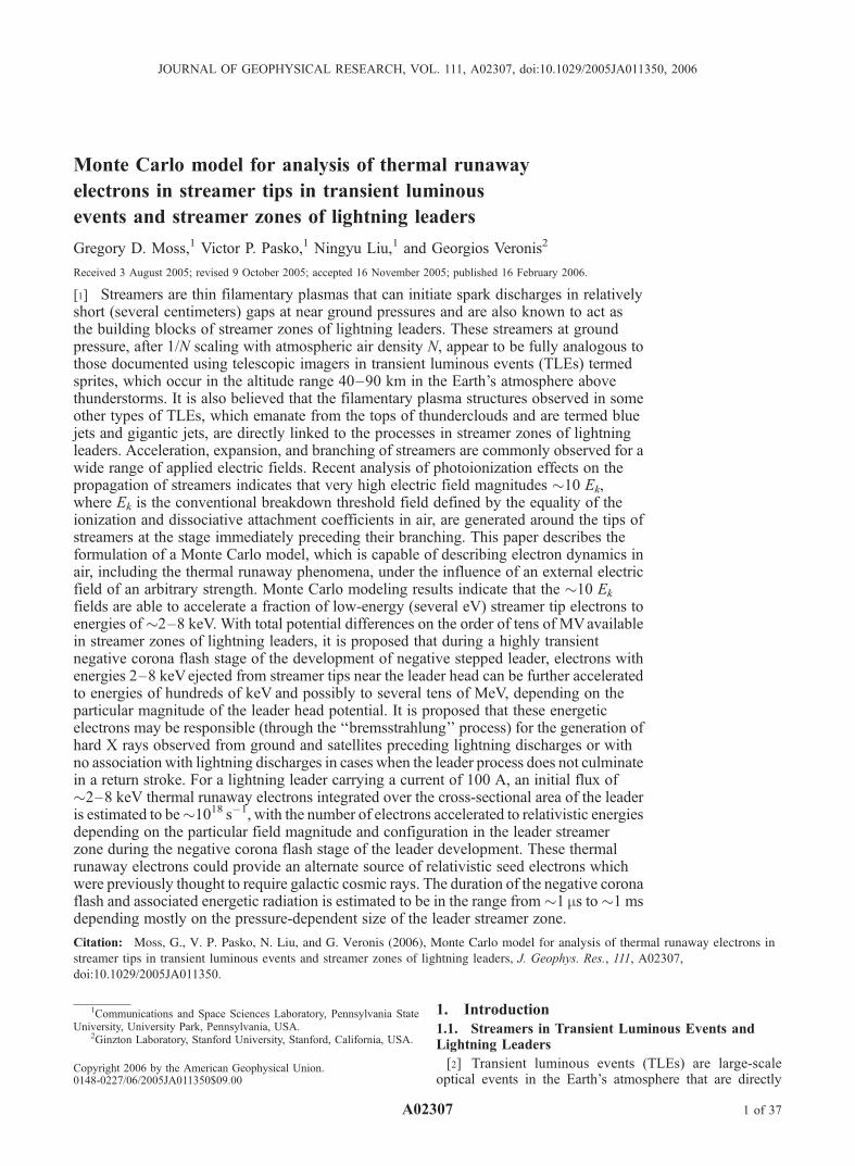
ally 15,000), is reached in a simulation, a remapping of theelectron assembly is performed to reduce the total numberof particles to another predetermined number, Tt (usually8000), with each new particle being assigned a new particleweight to reflect how many electrons the particle represents.Given the nature of the electron energy distribution functionin air (i.e., the bulk of the electron distribution is maintainedat lower energies with a small number of electrons constitut-ing a high-energy tail), measures must be taken to maintainappropriate resolution in the high-energy tail of the distribu-tion especially in the study of runaway phenomena. To dothis, the initial particles Nt are first sorted in order ofincreasing energy. After sorting the particles, they are thenpartitioned into two groups, one group representing the low-energy body N1 of the distribution and another representingthe high-energy tail N2 (see Figure 10). The first low-energygroup of particles is remapped such that the weights ofadjacent particles in energy space (Wj andWj+1) are combinedinto one particle with a new particle weight W 0

j such that

W 0j ¼ Wj þWjþ1: ð45Þ

The new particle assumes the properties of the jth particlesuch that enew = ej, vk,new = vk,j, and v?,new = v?,j, which is anadequate assumption since the energy difference betweentwo adjacent particles in energy space after the sorting willbe small in the low-energy body of the electron energy

Figure 10. Schematic example of a particle remappingcalculation reducing the total number of particles from Nt =15,000 to Tt = 8000.


13 of 37

A02307

distribution. This results in the total number of particles inthe low-energy region being reduced from N1 to T1 (usually7000) particles. The high-energy tail group is thenremapped 1:1 to ensure enhanced resolution at high electronenergies such that

W 0j ¼ Wj ð46Þ

for all particles in the tail and N2 = T2 (usually 1000). Theprocedure is repeated each time the particle count in asimulation exceeds Nt and is validated by comparing theelectron energy distribution function from before and afterthe remapping events.[50] For simulations when the spatial distribution of elec-

trons must also be considered, as with the one-dimensionaltreatment of runaway electrons in a streamer tip (section 4),remapping the particle assembly becomes slightly morecomplicated. When remapping occurs, the particles are firstsorted according to increasing position along the z-axis. Theparticles are then divided into equally spaced spatial bins(usually 10) and then sorted in order of increasing energywithin each bin. The remapping of particles is thenperformed within each bin according to the same 1:2 forlow-energy and 1:1 for high-energy particles as discussedin the previous paragraph (see Figure 11). The remapping

scheme is validated by comparing the electron energydistribution function before and after a remapping event.

2.7. Model Initialization and Execution

[51] Figure 12 shows a flow chart representing theexecution of the Monte Carlo model. First, the user mustinput basic simulation parameters such as the initial numberof particles to be used (usually 8000), the applied electricfield strength, the length of the simulation, the fractionalcomposition of the gas mixture (i.e., 78.11% N2, 20.91%O2, and 0.98% Ar), and the number of particles at which theparticle assembly will be remapped (usually 15,000, seesection 2.6).[52] After the input parameters are entered, the model can

then calculate the initial electron distribution and definenecessary quantities to be used throughout the simulationsuch as the collision frequency and the size of the time step.The initial electron set is normally assigned a Maxwellianvelocity distribution function [Chen, 1984, p. 226; Birdsalland Langdon, 1991, p. 390] corresponding to an initialelectron temperature of Te = 5800 K (i.e., 0.5 eV). Toachieve a Maxwellian velocity distribution, each electron isassigned a vx, vy, and vz velocity component. Using the errorfunction, defined by

erf vð Þ ¼ 2ffiffiffip

pZ v

0

e�t2dt; ð47Þ

where in the context of the present problem 0 � v � 5 is a

generic range normalized by thermal velocity vth =

ffiffiffiffiffiffiffiffi2KTem

q,

the normalized vx component of an electron’s velocity canbe related to a uniform random number Rj between 0 and 1from the relationship [e.g., Birdsall and Langdon, 1991,p. 390]

Rj ¼2ffiffiffip

pZ vx

0

e�t2dt ¼ erf vxð Þ: ð48Þ

Similarly, the normalized vy and vz velocity componentscan also be found for each electron using equation (48).After assigning velocity components to half of the electronpopulation, the remaining electron velocities may be foundby mirroring the positive velocity components found fromequation (48) to the corresponding negative values. A truethree-dimensional (3-D) Maxwellian distribution is thenarrived at by multiplying the normalized vx, vy, vzcomponents of each electron by the thermal velocity vth.The 3-D distribution is then transformed to parallel andperpendicular velocity components for use in the MonteCarlo simulation as

vk ¼ vz ð49Þ

v? ¼ffiffiffiffiffiffiffiffiffiffiffiffiffiffiv2x þ v2y

q; ð50Þ

assuming an electric field in the z-direction (see Figure 9).[53] The total collision frequency nt(e), the collision

frequency for each process nj(e), and the maximum collisionfrequency nmax are calculated from the cross section data

Figure 11. Schematic example of a particle remappingcalculation when the spatial position of particles isconsidered.


14 of 37

A02307

sets (section 2.1) prior to the simulation to reduce compu-tation time. These values are then loaded into the simulationat runtime and used to calculate the time step (equation (32))and to determine if and what type of collision an electronexperienced in a time step as outlined in Figure 6. Inaddition, the differential scattering cross section data dis-cussed in section 2.1 is also tabulated prior to execution,allowing for convenient table lookups during the simulationto determine electron scattering after a collision.[54] Each particle is then stepped through the ‘‘Null

Collision Method’’ as summarized in Figure 6 to determineif it experienced a real collision in the time step, and if so,what type of collision occurred. If the electron experienceda real collision, the electron’s energy and trajectory are

updated corresponding to the type of collision as discussedin section 2.5. After all electrons have been stepped throughthe collisional part of the model, each electron’s parallelvelocity (vk) is updated to reflect the acceleration due to theelectric field E during the time step Dt using a first-orderfinite-difference representation of Newton’s second lawas vk

new = vkold �qe

mEDt.

[55] Diagnostic data is then saved to file to allow fortime-dependent analysis of certain quantities to be calcu-lated (section 2.8) after the simulation is complete (i.e.,mean energy versus time, drift velocity versus time, ratecoefficients, etc.). If a certain number of particles hasbeen reached, the particle assembly is then remapped(section 2.6) in order to maintain reasonable computation

Figure 12. Flow chart depicting the execution of the Monte Carlo model.


15 of 37

A02307

times. It is then checked to determine if the simulationhas converged to a steady state (i.e., mean energy anddrift velocity remain constant over a certain time span). Ifthe simulation has converged, then the simulation data issaved to file; if not, the simulation returns to thebeginning of the next time step and the procedure isrepeated until a converging solution is reached.

2.8. Model Diagnostics

[56] The electron energy distribution n(e) (normalized asR10

n(e) de = 1) is obtained by sampling and averaging theelectron assembly at several moments of time as thesimulation reaches equilibrium. At each moment of time,the particles are divided into equally spaced bins along theenergy e axis and the particles weights Wj are summed toobtain the true number of electrons existing in each energybin. The resulting functions are then normalized and aver-aged in time and the final distribution function n(e) isnormalized again

n eð Þ ¼ n eð ÞZ emax

0

n eð Þdeð51Þ

to ensure thatR emax

0n(e) de = 1, where emax is the maximum

electron energy.[57] The electron mean energy can be simply calculated

by summing the energy of each particle included in thesimulation

hei ¼

XNt

j¼1Wj ej

nt; ð52Þ

whereWj and ej are the weight and energy of the jth particle,respectively, Nt is the total number of particles in the

simulation, and nt is the total number of electrons which canbe defined as

nt ¼XNt

j¼1

Wj: ð53Þ

This calculation is performed at every time step and theresult is used to determine if the simulation has reached anequilibrium state. Likewise, considering that the electronvelocity is represented by its parallel and perpendicularvelocity (Figure 9a, equations (38) through (40)), thedrift velocity can be found by

vd ¼

XNt

j¼1Wj vk;j

nt: ð54Þ

The electron mobility can then be calculated as

me ¼vdj jEj j : ð55Þ

[58] After a simulation has reached a steady state, the ratecoefficients for various collision processes can be deter-mined by simple counting procedures over a given timeinterval. First, consider a dummy variable Ci(t) which isused to count the occurrences of an ionization process overa given time interval. Each time an ionization collisionoccurs, the counter Ci(t) is incremented as

Ci tð Þ ¼ Ci tð Þ þWj; ð56Þ

where Wj is the weight of the particle experiencing thecollision. The rate coefficient for this ionization process canbe obtained by selecting two moments in time t1 and t2 after

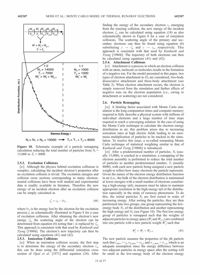
Figure 13. (a) Electron energy distribution in N2 at E/N = 300 Td as presented by Kunhardt and Tzeng[1986a] (where the dotted line corresponds to results obtained when electron scattering is considered tobe isotropic and the solid line corresponds to results obtained when electron scattering was determinedusing differential cross sections from experiment and theory) and (b) as calculated in the present work.Figure 13a is reprinted with permission from [Kunhardt and Tzeng, 1986a]. Copyright 1986 by theAmerican Physical Society.


16 of 37

A02307

the simulation has reached an equilibrium state. Theionization rate coefficient can then be calculated as

ni ¼Ci t2ð Þ � Ci t1ð ÞZ t2

t1

nt tð Þdt; ð57Þ

where nt(t) is the total number of electrons as a function oftime defined by equation (53). This calculation can beapplied to any collision process (e.g., na2 two-bodyattachment, B3�g excitation of N2, C

3�u excitation of N2,etc.) for which a corresponding counter Ck(t) wasmaintained during the simulation. The meaning of theprocedures defined by equations (56) and (55) can best beunderstood by direct integration of the dynamic equationsdescribing the growth of the total number of electrons ntdue to ionization

dnt

dt¼ nint ð58Þ

or the growth of the total number of excited species nk dueto impact excitation by electrons

dnk

dt¼ nknt : ð59Þ

3. Zero-Dimensional Calculations andModel Validation

[59] To test the precision and accuracy of the newlydeveloped Monte Carlo model, zero-dimensional simula-tions were performed to compare with previously publishedMonte Carlo models, numerical solutions of the Boltzmannequation, and existing experimental data. For these compar-

isons the spatial distribution of electrons was ignored withonly parallel (vk) and perpendicular (v?) velocity compo-nents with respect to the applied electric field beingconsidered.

3.1. Comparisons With Previous MonteCarlo Model Results

[60] Figures 13, 14, and 15 show calculation comparisonsof the electron energy distribution function n(e) in N2 gas atground pressure from the current Monte Carlo model andthe Monte Carlo model of Kunhardt and Tzeng [1986a]. Foreach simulation an assembly of 8000 electrons with aninitially Maxwellian velocity distribution (electron temper-ature Te = 0.5 eV) was placed under the influence of auniform electric field and the simulation was performeduntil the assembly reached an equilibrium state. High-energy (e > 500 eV) angular scattering of electrons wasdetermined using equation (14) and remapping was per-formed when the total number of particles reached a valueNt > 15,000.[61] The electron energy distribution function is shown

for E/N values of 300 Td and 1500 Td (1 Td = 10�17 Vcm2). Figures 13a and 14a are results presented byKunhardt and Tzeng [1986a] corresponding to ‘‘model3’’ of their study in which elastic and inelastic collisionswere taken to be anisotropic and differential scatteringcross sections were obtained from experiment and theory.For the same scattering consideration, the results of thepresent model are shown in Figures 13b and 14b. Theenergy distributions shown in Figures 13a and 13bdemonstrate the same shape characteristics with the sharppeak in the number of electrons existing below 2 eVbeing 15% lower in the current calculations. This ismost likely due to the use of updated collision crosssection and differential cross section data in the currentmodel, as compared to Kunhardt and Tzeng [1986a].Similarly, Figures 14a and 14b also demonstrate the same

Figure 14. (a) Electron energy distribution in N2 at E/N = 1500 Td as presented by Kunhardt and Tzeng[1986a] (where the dotted line corresponds to results obtained when electron scattering is considered tobe isotropic and the solid line corresponds to results obtained when electron scattering was determinedusing differential cross sections from experiment and theory) and (b) as calculated in the present work.Figure 14a is reprinted with permission from [Kunhardt and Tzeng, 1986a]. Copyright 1986 by theAmerican Physical Society.


17 of 37

A02307

overall shape with a 7% lower peak value for the samereason. It can be seen that for E/N = 1500 Td the high-energy tail of the distribution extends to energies �100 eVand with further inspection of the tail, Figures 15a and 15bshow the population of thermal runaway electrons existingat energies �100 eV. The nonsmooth appearance of thedistribution seen in Figure 15 is due to the small numberof particles being sampled in these high-energy regions.Figure 15a corresponds to ‘‘Case 2’’ presented by Tzengand Kunhardt [1986] in which the energy of secondaryelectrons emerging from ionizing collisions is determinedfrom the differential ionization cross section of Opal et al.[1971] as discussed in section 2.3. Kunhardt and Tzeng[1986a] emphasize that the treatment of angular scattering

can have a great effect on the electron energy distributionfunction. While the variations displayed in the low-energyportion of the distribution are small, assumptions aboutangular scattering of electrons can significantly inhibit orpromote the development of runaway as will be shown insections 3.3, 4.1, and 4.2.

3.2. Comparisons With ELENDIF, ExperimentalResults, and Previous Models

[62] Figures 16, 17, and 18 show the energy distributionfunction n(e), mean energy hei, phase space velocitydistribution, and drift velocity vd of electrons in an airmixture at ground pressure consisting of 78.11% N2,20.91% O2, and 0.98% Ar under the influence of applied

Figure 15. (a) High-energy tail of the electron energy distribution in N2 at E/N = 1500 Td as presentedby Tzeng and Kunhardt [1986] and (b) as calculated in the present work. Figure 15a is reprinted withpermission from [Tzeng and Kunhardt, 1986]. Copyright 1986 by the American Physical Society.

Figure 16. (a) Electron energy distribution function, (b) electron mean energy, (c) electron velocitydistribution in phase space, and (d) electron drift velocity in air under the influence of an electricfield E = 0.3Ek.


18 of 37

A02307

electric fields E = 0.3Ek, E = 1.2Ek, and E = 20Ek,respectively, where Ek is the previously defined conven-tional breakdown field. As in section 3.1, an assembly of8000 electrons with an initially Maxwellian velocitydistribution (electron temperature Te = 0.5 eV) was used.Equation (14) was utilized to determine high-energy (e >500 eV for collisions with N2 and e > 1000 eV forcollisions with O2 and Ar) angular scattering of electronsand remapping was performed when the number ofparticles reached Nt > 15,000.[63] The electron distribution function in Figures 16a,

17a, and 18a are compared to results obtained from theELENDIF Boltzmann equation solver [Morgan andPenetrante, 1990]. It can be seen that for low field valuesE = 0.3Ek and E = 1.2Ek the energy distributions obtainedfrom the current Monte Carlo model are in excellentagreement with results obtained from the ELENDIF soft-ware with differences of <5% and 5%, respectively.Also, Figures 16a and 17a provide an excellent insight intothe dynamic friction force in air (section 1.2, Figure 2).Figure 16a shows that the majority of the electron popu-lation under the influence of an electric field E = 0.3Ek ismaintained at energies <2 eV. Electrons are held at theselow energies because of the N2 vibrational processes withthreshold energies ranging from 0.28 eV to 2.35 eV (seeTable 1) constituting the ‘‘first bump’’ of the dynamicfriction force (Figure 2). The electrons lose more energyto these vibrational collisions than they gain from theapplied electric field. For an electric field E = 1.2Ek,however, it becomes possible for electrons to gain moreenergy from the electric field than they lose to thesevibrational processes. As can be seen in Figure 17a, alarge population of electrons remain at energies <2 eV dueto vibrational collisions, but a significant number is able

to penetrate through the vibrational barrier and is accel-erated to energies >2 eV. These electrons, however, donot accelerate to higher energies because of the increasedcollision frequency and energy loss corresponding to the100 eV ‘‘hump’’ of the dynamic friction force (Figure 2).Figure 18a shows the energy distribution of electronswhen an electric field E = 20Ek, much greater than thethermal runaway field Ec, is applied and a large percent-age of the total electron population is accelerated toenergies >100 eV. It can also be seen in Figure 18a thatthe two-term spherical harmonic expansion [e.g., Raizer,1991, chap. 5] used in the ELENDIF solution fails at thishigh electric field value and the Monte Carlo and ELENDIFresults no longer agree. Figures 16b, 17b, and 18b showthe simulation reaching an equilibrium state as the meanenergy converges to a constant value for each of theelectric field cases and Figures 16d, 17d, and 18d showthe average drift velocity of electrons also converging. Itcan be seen from Figure 18b that the mean energy ofelectrons is only �60 eV, showing that even for anextremely high electric field E = 20Ek, it is still verydifficult for electrons to accelerate to energies >100 eVand only a small fraction of them becomes runaway.Figures 16c, 17c, and 18c show the phase space velocitydistributions of particles in the system. Figures 16c and 17cconfirm that for electric fields E = 0.3Ek and E = 1.2Ek thevelocity distributions remain largely isotropic, thus justify-ing the two-term spherical harmonic expansion used in theELENDIF solution. On the contrary, Figure 18c showsthat for E = 20Ek the velocity distribution becomes highlyanisotropic because of thermal runaway electrons andtherefore the two-term spherical harmonic expansion canno longer be utilized in the solution of the Boltzmannequation.

Figure 17. (a) Electron energy distribution function, (b) electron mean energy, (c) electron velocitydistribution in phase space, and (d) electron drift velocity in air under the influence of an electric field E =1.2Ek.


19 of 37

A02307

[64] Figures 19 through 22 show results of Monte Carlomodel calculations compared to results obtained fromELENDIF, experimental swarm parameter measurementsin dry air reported by Davies [1983], and from relatedanalytical model approximations proposed by Aleksandrovet al. [1995] and Morrow and Lowke [1997] for a range ofapplied electric fields. Figure 19a shows that the electronmean energy calculated by the Monte Carlo model agreeswell with the ELENDIF Boltzmann code at most electricfields, demonstrating only a slight deviation of 25% atE = 6 � 107 V/m. The Monte Carlo calculation ofelectron mobility me shown in Figure 19b shows excellentagreement with the experimental values of Davies [1983]and ELENDIF calculations for electric fields ranging

from E = 5 � 105 to E = 1 � 107 V/m butdemonstrates a percent difference of 38% with ELENDIFcalculations at E = 6 � 107 V/m. However, the MonteCarlo mobility calculation agrees well with the modelapproximation of Morrow and Lowke [1997] for electricfields >1�107 V/m. It can be seen in Figure 20a that theionization coefficient calculated by the Monte Carlomodel demonstrates excellent agreement with experimentalmeasurements [Davies, 1983], ELENDIF calculations, andthe model of Aleksandrov et al. [1995] at all electric fieldvalues, but displays a difference of 68% with the modelof Morrow and Lowke [1997] at E = 6 � 107 V/m. Thevalues calculated and reported for the two body attachmentcoefficient na2 vary greatly, as can be seen in Figure 20b.

Figure 19. (a) The electron mean energy hei and (b) electron mobility me in air as a function of appliedelectric field.

Figure 18. (a) Electron energy distribution function, (b) electron mean energy, (c) electron velocitydistribution in phase space, and (d) electron drift velocity in air under the influence of an electric fieldE = 20Ek.


20 of 37

A02307

The results of na2 calculated by the Monte Carlo modelagree well with the model of Aleksandrov et al. [1995] andELENDIF calculations for electric fields >2 � 106 V/mbut are significantly higher at fields <2 � 106 V/m. TheMonte Carlo va2 calculations demonstrate a difference ofup to 58% compared to experimental values, with thesharp decline in the na2 values of Davies [1983] for E >3 � 106 V/m not being reproduced by Monte Carlo andELENDIF solutions. This is most likely due to the pres-ence of collisional detachment, which is not included in theMonte Carlo and ELENDIF calculations, impacting theexperimental results [Davies, 1983]. It also can be seenfrom Figures 21 and 22 that the excitation coefficients ofthe B3�g and C3�u states of N2 and the B2Su

+ state of N2+

obtained from the Monte Carlo model agree well withresults obtained from ELENDIF at high electric fieldvalues but show better agreement with the calculation ofAleksandrov et al. [1995] at lower electric fields. The B2Su

+

optical excitation coefficients shown in Figure 22 werecalculated by obtaining the ionization rate coefficients ofN2 from the Monte Carlo model (see section 2.8), ELENDIFcalculations, and approximations of Aleksandrov et al.[1995], and then multiplying the resulting coefficients by abranching ratio (fB = 0.145) presented by Van Zyl andPendleton [1995].[65] These results indicate that although the two-term

spherical harmonic expansion is not generally valid at highelectric field values, the above rate coefficients obtainedfrom ELENDIF remain valid for electric fields up to 6 �107 V/m (20Ek). The differences between Monte Carloand ELENDIF calculations of electron mean energy andmobility at high electric fields are most likely due to theelectron distribution becoming anisotropic.[66] We note that results of Figures 19 through 22 are

presented in a reduced form using the ratio of the air densityat ground pressure N0 = 2.688 � 1019 cm�3 to the density at

Figure 20. (a) The total ionization coefficient ni and (b) O2 two-body attachment coefficient na2 in airas a function of applied electric field.

Figure 21. (a) The first positive band system of N2 (B3�g state) and (b) second positive band system of

N2 (C3�u state) optical excitation coefficients in air as a function of applied electric field.


21 of 37

A02307

any other pressure N. This scaling is justified by thesimilarity properties of gas discharges [e.g., Liu and Pasko,2004, and references therein] and can be directly used forcalculation of physical quantities at any other air density Nof interest.[67] A MATLAB function, based on ELENDIF solutions,

was used in the plotting of Figures 19 through 22. Thisfunction allows the calculation of many physical quantitiesand rate coefficients as a function of the reduced electricfield in air and is freely available to readers as a supplementto this paper at http://pasko.ee.psu.edu/air.

3.3. Runaway Electron Development

[68] To examine the development of runaway electronsfor various electric fields, simulations were conducted toperform direct comparisons with recent results presentedby Bakhov et al. [2000]. An initial assembly of 1 eVelectrons (N0 = 5000) with velocities unidirectional withthe electric force was placed in N2 gas at ground pressurewith applied electric fields of 400 kV/cm, 350 kV/cm, and325 kV/cm, and simulated for times of t = 1 ns, t = 6 ns,and t = 25 ns, respectively. In accordance with Bakhov etal. [2000], the following nitrogen electronic states wereconsidered (see Table 1): A3Su

+ (v = 5–9 and v = 10+),B3�g, W

3Du, B03Su

�, C3�u, w1Du, a

1�g, and the sum ofthe remaining singlet states (threshold e = 13 eV).Elastic and ionization collisions were also considered;however, while ionization was considered as an energyloss mechanism, secondary electrons were not added to theparticle assembly. When electrons reached an energy equalto emax = 4000 eV, they were considered to be runawayand removed from the simulation.[69] Figure 23 shows results of the Monte Carlo model

of Bakhov et al. [2000], in which angular scattering ofhigh-energy electrons after elastic and ionization collisionsis determined from the electron data library (EEDL)[Perkins and Cullen, 1994] and is adopted to be forwardafter excitation collisions. Figure 24 shows similar results

calculated by the Monte Carlo model discussed in thispaper, where high-energy angular scattering has beendetermined by the differential scattering cross sectionapproximation published by Kol’chuzhkin and Uchaikin[1978] (equation (14), Figure 24a) and the modified Ruth-erford cross section introduced in this paper (equation (16),Figure 24b). A direct inspection of the atomic nitrogendata presented in the EEDL library at selected energies of1, 2.5, and 5 keV indicates that among the modelsdiscussed in section 2.2 of this paper the correspondingdifferential cross sections are closest to the approximationgiven by equation (9).[70] Recalling that low-energy (e < 500 eV) electron

scattering is determined by the experimentally determineddifferential cross sections listed in Table 5 for all simula-tions, the only difference between the simulations ofFigure 24a and 24b is the differential scattering crosssection used for energies >500 eV. It is obvious fromthe major differences shown in Figures 24a and 24bthat the high-energy scattering of electrons is critical inthe development of electron runaway. Comparison ofFigures 4c and 4d show that the differential scatteringcross section calculated from equation (16) possesses amuch larger forward scattering characteristic than that ofequation (14) for all electron energies. The effect of thisforward scattering on the development of runaway elec-trons is well illustrated in Figure 24 and by comparingFigures 23 and 24 it can be seen that results obtained byBakhov et al. [2000] using EEDL data are similar to thoseobtained with our model using the differential scatteringcross section calculated from equation (16). It can also beseen from Figure 24a that assuming forward scatteringafter excitation collisions drastically increases the produc-tion of runaway electrons when equation (14) is used. Thisis not the case when the same assumption is used withequation (16) since equation (16) already possesses astrong forward scattering characteristic.[71] Also of interest are the considerable differences in

Figures 24a and 24b when forward scattering after excita-tion collisions is assumed. Since excitation collisions areforward for both cases, the elastic and ionization collisionsmust be responsible for the large differences in runaway

Figure 22. First negative band system of N2+ (B2Su

+ state)optical excitation coefficient in air as a function of appliedelectric field.

Figure 23. The fraction Nr/N0 of the initial electronassembly to reach energies �emax = 4000 eV as calculatedby Bakhov et al. [2000]. Copyright 2000 by the IEEE.


22 of 37

A02307

electrons observed. While elastic collisions are the domi-nant collision process at low electron energies, the differ-ences in Figures 24a and 24b are most likely due to thehigh-energy scattering of the primary electron afterionizing collisions. This leads to an interesting conclu-sion that the high-energy angular scattering from ionizingcollisions is much more important in the development ofelectron runaway than high-energy scattering from excita-tion collisions.

4. One-Dimensional Streamer Tip Simulations

[72] In this section the Monte Carlo model discussed inthe previous sections is modified to study the production ofrunaway electrons in streamer tips. The model calculationsare conducted for a case of streamers at an air pressurecorresponding to 70 km altitude (p = 0.05 Torr). Owing tothe similarity properties of streamers [Liu and Pasko, 2004,and references therein] the reported results can be general-ized to air streamers existing in systems at any pressure ofinterest (i.e., those discussed in section 1.1). The electricfield is assumed to be unidirectional with the z-axis andelectron velocities are still considered in terms of theirperpendicular (v?) and parallel (vk) components withrespect to the applied electric field (see Figure 9). Theelectron positions were tracked along the z-axis and updatedat the end of each time step according to

z0 ¼ zþ vk Dt; ð60Þ

where z is the initial position of the electron and z0 is thenew position. All simulations are performed in an airmixture consisting of 78.11% N2, 20.91% O2, and 0.98% Arutilizing the cross sections listed in section 2.1.

4.1. Stationary Streamer Tip Model

[73] To demonstrate the importance of high-energy angu-lar scattering in the development of runaway electrons in a

streamer tip, four different cases utilizing the differentialscattering cross section of Kol’chuzkin and Uchaikin [1978](equation (14)) and the modified Rutherford cross sectionof equation (16) were considered. It can be seen fromFigures 4 and 5 that these two cross sections possess verydifferent scattering properties which greatly influence thedevelopment of runaway electrons as shown in Figure 24.As in section 3.3, simulations were performed for bothcross sections with and without the assumption of forwardscattering after excitation collisions.[74] The strong electric field associated with a streamer

tip immediately preceding branching (Figure 1) is approx-imated by a 10 Ek square pulse spanning 1 m in z-spaceand is placed in various ambient electric fields Eamb

(Figure 25a). We note that in accordance with similaritylaws [e.g., Liu and Pasko, 2004], the streamer spatial scales(i.e., width of the streamer tip) and electric fields scale withair density N as �1/N and �N, respectively. Therefore themaximum energy, which can be gained by electrons in thestreamer tip, remains the same for similar streamers atdifferent air densities, or pressures (assuming constant gastemperature). The magnitude of the electric field in thestreamer tip (10Ek = 2170 V/m) and the tip width (1 m)shown in Figure 25 correspond to a model streamer at 70 kmaltitude (Figure 1). As mentioned above, all results reportedin this section can be easily generalized to streamers at otheraltitudes (pressures) of interest using similarity laws.[75] The two quantities of interest are the runaway pro-

duction rate nrun [1/s] and the runaway flux Grun [1/m2/s].The runaway production rate nrun is defined as the rate atwhich electrons inside the streamer tip volume reachenergies greater than a predefined runaway energy erun.The runaway flux Grun represents the number of electronswith energies greater than erun which pass through a unitarea 1 m in front of the streamer tip per unit time. Thedistance of 1 m in front of the streamer tip was arbitrarilychosen such that the focus of our study is placed on thenumber of runaway electrons produced by streamer tips and

Figure 24. The fraction Nr/N0 of the initial electron assembly to reach energies � emax = 4000 eVcalculated by the Monte Carlo model developed in this paper with high-energy angular scatteringdetermined from (a) equation (14) and (b) equation (16). Results are shown with and without theassumption of forward scattering after high-energy (e > 500 eV) excitation collisions.


23 of 37

A02307

not the future evolution of these electrons. Figure 26 showsthe geometry and a sample calculation of nrun and Grun for acase when the ambient field is assigned a value of Eamb =4Ek and equation (16) was used to determine all angularscattering. Plotting the cumulative number of runawayelectrons generated within the streamer tip volume Nrun

and the number of runaway electrons to pass through theunit area 1 m ahead of the streamer tip Nrun-flux as functionsof time, allows the rates n0run and G0

run to be calculated (seeFigure 26). These rates may then be scaled to realisticvalues nrun and Grun corresponding to a streamer tip electrondensity ne at 70 km of 1012 m�3 [Liu and Pasko, 2004] as

nrun ¼ne

ntip� n0run ð61Þ

Grun ¼ne

ntip� G0

run; ð62Þ

where ntip is the electron density of the streamer tip in thesimulation (see Figure 26). These values can then begeneralized to streamers at other altitudes and pressuresnoting the similarity properties of streamers [Liu andPasko, 2004, and references therein] following therelationship ne = ne0

N2

N20

, where ne0 = 2 � 1020 m�3 is

the reference streamer density at ground level, and N0 andN are defined in the paragraph before last of section 3.2.[76] After performing a number of test simulations, it was

determined that n0run and G0run are independent of the 0.5 m

Eamb field region behind the streamer tip (Figure 25a), thusallowing the simulation domain to be reduced to twoelectric field regions (Figure 25b). This simplificationallows for more electrons to be placed in the 10 Ek streamertip region, which improves the statistics of the n0run and G

0run

calculations.[77] In order to accurately represent the constant electron

density of a propagating streamer tip [e.g., Liu and Pasko,2004], the electron density was kept constant over the 10 Ek

region throughout simulations using ten spatial bins(Figure 25c). After performing several test simulations, theelectron density in the ambient field region namb was foundto have no effect on nrun and Grun and therefore was allowedto be variable. At the end of each time step, the density ofelectrons in each of the ten bins (nbin) is calculated. Theelectron density in each bin is then compared with thedesired constant ntip to determine if there are too many ortoo few electrons in the bin. If nbin > ntip, then nbin � ntipelectrons with energies less than 10 eV (ensuring that arunaway electron is not being repositioned) are randomlyselected from the bin and 1 m is added to their current z-position thus moving them into the namb region. If nbin < ntip,then ntip � nbin electrons with energies less than 10 eV arerandomly selected from the namb region and placed at the leftboundary of the bin in question.[78] This formulation results in a constant total number of

electrons Ntip (see Figure 25c) being exposed to the highelectric field of the streamer tip at all times throughout thesimulation, but due to two-body and three-body attachmentcollisions with O2 (see Table 2) the total number ofelectrons in the low field region Namb decreases slightlyover time. Initial values of ntip are normally chosen to be150,000, 100,000, 75,000, 50,000, or 25,000 m�3 depend-ing on the resolution needed to obtain satisfactory statisticsfor various electric field and scattering cases, and namb isinitially 20,000 m�3 for all simulations.[79] It should be noted that while ionization is consid-

ered as an energy loss mechanism for primary electrons,secondary electrons are not added to the simulation of thestationary streamer tip, and the one-dimensional remappingof particles discussed in section 2.6 was not utilized in thesimulations. For an electric field of 10Ek the ionizationcoefficient is �7 � 1011 N

N0s�1 (see Figure 20), which

leads to an enormous multiplication of electrons. If thesesecondary electrons are added to the simulation, as withthe zero-dimensional model, the particle weights andelectron density grow at an extremely fast pace. This fastgrowth is believed to be an inaccurate representation of theactual physical system in which the electron density in thestreamer tip is dynamically maintained at relatively stablelevels. The focus of this study is therefore placed ondetermining the number of initially cold electrons out of

Figure 25. (a) and (b) The simplified electric field and(c) electron density configuration corresponding to amodel approximation of a streamer tip at 70 km used inone-dimensional Monte Carlo simulations.


24 of 37

A02307

a known constant electron density to reach runawayenergies. This evolution of individually tracked runawayelectrons can therefore be treated without consideration ofthe avalanche multiplication of electrons due to ionization.This assumption, however, relies heavily on the fact thatmost secondary electrons emerge from ionizing collisionswith low energies. Simulations have shown that a smallpercentage of secondaries do possess energies >200 eV,thus placing them over the ‘‘hump’’ of the dynamicfriction force (Figure 2). These high-energy secondariesentering an electric field �10 Ek have an increasedprobability of becoming runaway electrons and wouldimpact the values of nrun and Grun. Several simulationswere performed in which secondary electrons emergingfrom ionizing collisions with energies >200 eV wereadded to the simulation and values of Grun were observedto increase by 10%.

[80] The energy required for an electron to be consideredrunaway erun is directly determined from the dynamicfriction force of electrons in air (Figure 2). Figure 27ashows the values of erun corresponding to ambient electricfields of 1 Ek, 2 Ek, 3 Ek, 4 Ek, and 5 Ek. It can be seen fromFigure 2a that these ambient fields alone are not strongenough to overcome the friction force FD and acceleratelow-energy electrons to energies >100 eV. An electric fieldof 10Ek, however, falls above the peak of FD and itbecomes possible for electrons exposed to a 10 Ek fieldto be accelerated to energies >100 eV. In view of theelectric field configuration shown in Figure 25b, the10Ek streamer tip field extending over 1 m length issolely responsible for all runaway electrons producedduring a simulation, and the magnitude of the ambientfield Eamb defines the value erun. To better understand thisrelationship, consider a case with Eamb = 3 Ek depicted in

Figure 26. Simulation geometry and sample calculations of the runaway production rate nrun and therunaway flux Grun for a case at 70 km when Eamb = 4Ek, the streamer tip length is L = 1m, and thestreamer tip density used in the simulation is ntip = 25000 m�3.


25 of 37

A02307

Figure 27b. An electron emerging from the 10 Ek streamertip region into the ambient field region may be consid-ered to fall into one of three categories: the electron hasan energy e < erun, e � erun, or e > erun. If the electronhas not gained sufficient energy from the 10 Ek streamertip (e < erun), the electron’s motion will be dominated bycollisions and the friction force will cause the electron todecelerate to low energies. If the electron has gainedenough energy from the streamer tip such that e > erun,the probability of the electron colliding with neutralparticles has significantly decreased (FD < 3 Ek) andthe electron will continue to be accelerated to higherenergies by the 3 Ek ambient field. If the electron hasgained an energy e � erun, the electron may be acceler-ated to higher energies by the ambient field or return tolow energies depending on the collisions and angularscattering it experiences.[81] Table 7 lists the values of erun for various ambient

electric fields and the corresponding electron velocities. Itshould be noted that the maximum energy which anelectron experiencing no collisions could gain from the1 m long streamer tip (see Figure 26) with 10 Ek field at70 km is 2170 eV. We emphasize again that this energywill be exactly the same for similar streamers at anypressure/altitude of interest. This energy corresponds to anambient field of 2.32 Ek. Therefore it is impossible toachieve runaway electrons for ambient fields <2.32 Ek inthe simulations. In reality, when collisions are considered,electrons only gain a fraction of the total 2170 eV and norunaway electrons were observed in any simulations withambient electric fields 2.5 Ek. Simulations were thereforeperformed for ambient field values ranging from 2.5 Ek to5 Ek as shown schematically in Figure 25b.[82] We emphasize that changes in the width of the

model streamer and the magnitude of the tip electric fieldwould affect the numerical values of ambient fields atwhich runaway electrons can be sustained, and these

values can be easily evaluated using procedures outlinedabove.[83] Figures 28 and 29 show simulation results for the

runaway production rate nrun and the runaway flux out of thestreamer tip Grun for various Eamb values (Etip = 10 Ek for allsimulations). Figure 28a shows results obtained when high-energy angular scattering after all collisions was determinedusing equation (16), and Figure 28b shows the same caseexcept high-energy scattering after excitation collisions wasconsidered to be forward (c = 0). Figures 29a and 29bshow results for the same scenarios, respectively, utilizingequation (14) to determine high-energy scattering instead ofequation (16). The solid lines in both Figures 28 and 29 wereobtained using a spline interpolation between Monte Carlodata points.[84] The variations in nrun and Grun at different ambient

fields can be largely attributed to the runaway energy erunbeing variable with the ambient field (Table 7). For exam-ple, consider ambient fields of 5Ek and 3 Ek correspondingto erun = 630 eV and erun = 1515 eV, respectively. A muchlarger fraction of the electron distribution exists at energies>630 eV than at energies >1515 eV, thus explaining thenotable increase in nrun and Grun with the increase in

Figure 27. (a) The determination of the electron runaway energy erun using the dynamic friction forceand the ambient electric field and (b) the three possible scenarios of an electron exiting the 10Ek streamertip corresponding to an ambient electric field Eamb = 3Ek.

Table 7. Energy and Corresponding Velocity Required for an

Electron to Run Away in Various Ambient Electric Fields

Eamb/Ek erun, eV vrun, m/s

1 6839 4.90 � 107

1.5 3948 3.73 � 107

2 2663 3.06 � 107

2.32 2170 2.76 � 107

2.5 1960 2.63 � 107

3 1515 2.31 � 107

3.5 1214 2.07 � 107

4 1000 1.88 � 107

4.5 788 1.66 � 107

5 630 1.49 � 107


26 of 37

A02307

ambient field. We emphasize again that the generation ofrunaway electrons is entirely due to the 10 Ek streamertip field. If erun were assigned a constant value for allambient field cases, nrun would also remain constant forall ambient fields since the 10 Ek streamer tip remainsunchanged.[85] It should be noted that not all electrons which

achieve energies >erun can be considered true runawayelectrons. The direction in which the electrons are travelingwith respect to the electric field also plays a major role inrunaway development. Electrons traveling in a directionopposing the applied electric field gain additional energyfrom the electric field, whereas electrons traveling in thesame direction as the electric field lose energy. Therefore itis possible for electrons with energies >erun to have vkvelocity components in the same direction as the electricfield and subsequently be losing energy. Clearly, these

electrons do not fit the definition of runaway electrons sincethey are in fact losing energy to the electric field. Thisillustrates the reason why the angular scattering of electronsbecomes so important in the development of runawayelectrons. When electrons are subject to significant angularscattering, they are more prone to obtain a vk which is in thesame direction as the applied electric field. Adversely, ifelectrons scatter primarily forward after collisions (in thedirection of electron drift and opposing the direction of theelectric field), it becomes easier for them to becomerunaway electrons because they will always be gainingenergy from the applied electric field. In order to moreaccurately differentiate between true runaway electronswhich are traveling in the direction opposite to the electricfield and high-energy electrons which are traveling in thesame direction as the electric field, a filtering proceduremust be introduced into the simulations. Figure 30 shows

Figure 28. The runaway production rate nrun and the runaway flux Grun obtained from the Monte Carlomodel when equation (16) is used to describe high-energy electron scattering (a) without and (b) with theassumption of forward scattering after excitation collisions.

Figure 29. The runaway production rate nrun and the runaway flux Grun obtained from the Monte Carlomodel when equation (14) is used to describe high-energy electron scattering (a) without and (b) with theassumption of forward scattering after excitation collisions.


27 of 37

A02307

the calculation of two fluxes of high-energy electronsobtained from a model simulation, G0 which is leaving thestreamer tip at z = 1 m and Grun which was definedpreviously. The results shown in Figure 30 are for a casewhen Eamb = 4Ek, all angular scattering was determinedusing equation (16), and Ntip = 50,000. The differencebetween G0 and Grun arises due to the 1 m ambient fieldregion ahead of the streamer tip and the deceleration of afraction of high-energy electrons within it. As discussedabove, an electron exiting the streamer tip with an energye � erun may either continue to be accelerated to highenergies by the ambient electric field or be returned to lowenergies due to collisions possessing strong backscattercomponents. Therefore the ambient field region acts as afilter separating the two groups of electrons. An electronwhich still possesses an energy greater than erun aftertraveling 1 m in the ambient field region continues to gainmore energy from the ambient field than it lost to collisions,consequently obeying the definition of a runaway electronas presented in section 1.2. It can be seen from Figure 30that for this case only 39% of the electrons which achievedenergies >erun at the streamer tip (z = 1 m), still possessedenergies >erun after traveling through the 1 m ambient fieldregion, the other 61% of electrons being decelerated bycollisions in the ambient field region.[86] Generally, the difference between G0 and Grun

grows larger as the ambient field intensity increases(erun decreases). At low ambient fields (high erun) electrons

which achieve energies >erun and contribute to G0 are athigh enough energies such that they scatter predominantlyforward after collisions. Therefore a large fraction ofelectrons achieving these high energies will continue toscatter forward in the ambient field region and accelerateto higher energies, thus contributing to Grun. Adversely,for high ambient fields (low erun) electrons are counted asrunaway within the streamer tip at much lower energiesand do not possess the same forward scattering properties.Therefore a large number of these electrons will besubject to significant angular scattering upon enteringthe ambient field region and will decelerate to lowenergies bringing about a larger difference in G0 and Grun.[87] Table 8 lists the average energies of electrons which

were counted in the calculation of Grun and the maximumelectron energy observed of those electrons. It becomesclear by comparing the values listed in Table 8 with therunaway energies erun listed in Table 7 that a portion ofthe electrons which were accelerated to energies >erun bythe streamer tip continued to gain energy from theambient electric field outside of the streamer tip, thussatisfying the definition of a true runaway electron. Formost electric field cases, electron energies >2 keV wereobserved at the left boundary 1 m ahead of the streamertip. However, it should be noted that while many elec-trons counted in the calculation of Grun sustained energiessignificantly greater than erun, some electrons still pos-sessed energies �erun and therefore may be decelerated tolow energies by collisions at distances greater than 1 mahead of the streamer tip. The average values listed inTable 8 are dependent on the number of electrons includedin the simulation. Since various electron densities wereused for different ambient field and scattering cases (i.e.,statistics are generally better for higher ambient fields), theaccuracy of the values listed in the tables may vary with theambient field.[88] One of the most interesting aspects of Figures 28

and 29 is the existence of a cutoff electric field at whichnrun and Grun rapidly drop to zero. In Figure 28a, in whichequation (16) was used to determine all high-energyangular scattering, the cutoff fields are Eamb 2.5Ek fornrun and Eamb 2.55Ek for Grun. When excitation colli-sions are assumed to be forward for the same case, thecutoff electric field for both nrun and Grun is Eamb 2.5Ek

as can be seen in Figure 28b. This would suggest that theassumption of forward scattering after excitation collisionsdoes not affect the cutoff electric field of the runawayproduction rate nrun but does impact the cutoff field of therunaway flux Grun. It can also be seen from Figures 28aand 29a that at high electric fields (>Eamb = 3Ek), theforward scattering assumption has a minimal effect on themagnitude of nrun and Grun, possessing a maximumpercent difference of 14% and 19%, respectively.However, for electric fields Eamb = 3Ek, the percentdifferences between Figures 28a and 29b are 65% fornrun and 137% for Grun, demonstrating that angularscattering after excitation collisions plays a larger rolewhen lower ambient fields (higher erun) are applied.[89] Similarly, Figure 29a, in which equation (14) was

used to determine all high-energy angular scattering,exhibits cutoff electric fields of Eamb 2.6Ek and Eamb

3Ek for nrun and Grun, respectively. When scattering after

Figure 30. The flux of electrons with energies >erun at theedge of the streamer tip G0 and the runaway flux ofelectrons 1 m in front of the streamer tip Grun as calculatedfrom a simulation with Eamb = 4Ek, angular scattering ofelectrons after all collisions determined by equation (16),and Ntip = 50,000.


28 of 37

A02307

excitation collisions is assumed to be forward, the cutofffield of Grun decreases from Eamb 3Ek to Eamb 2.6Ek

while the cutoff field of nrun remains Eamb 2.6Ek.Similar to Figure 28, the differences between the nrunvalues of Figures 29a and 29b are relatively small, witha maximum difference of 83%. On the contrary, thedifference between the Grun values plotted in Figures 29aand 29b is dramatic, possessing percent differences >100%at all electric field values. The fact that differencesbetween Figures 29a and 29b are much greater than thedifferences between Figures 28a and 28b demonstratesthat assuming forward scattering after excitation collisionshas a much greater effect on runaway electrons whenequation (14) is used to calculate high-energy angularscattering and corresponds well with the results reportedin Figure 24.[90] As discussed in section 2.2 and shown in Figure 24,

the differential scattering cross section used to describehigh-energy electron scattering can have a major impacton the development of runaway electrons. This can furtherbe seen by comparing the results of Figures 28a to 29aand the results of Figures 28b to 29b. As discussed above,the most notable difference is the variation in the cutoffelectric field at which nrun and Grun rapidly drop to zero. Inaddition to the variation in the cutoff electric field, themagnitudes of nrun and Grun are noticeably greater whenthe differential cross section of equation (16) is used.Comparing Figures 28a to 29a, at ambient electric fields�3.5Ek, the values of Grun in Figure 28a are 25 to45 times greater than those of Figure 29a. When scatteringafter excitation collisions is assumed to be forward, theGrun values of Figure 28b at ambient fields �2.8Ek are8 to 16 times those of Figure 29b. The differences innrun are not as drastic, with a maximum percent differencebetween the values shown in Figure 28a and Figure 29a of150% at Eamb = 2.8 Ek decreasing to 40% at Eamb =5 Ek. Similarly, comparing Figures 28b to 29b results inpercent differences of 140% at Eamb = 2.8 Ek decreasingto 25% at Eamb = 5 Ek. Since the differences in nrun arenot as great as those in Grun, one may conclude that theangular scattering of electrons once they enter the ambientfield region ahead of the streamer tip is much morecritical for sustaining runaway electrons than the scatter-ing of electrons within the high field streamer tip.[91] The difference in nrun between the two cross section

cases (equations (14) and (16)) decreases at higher electricfield due to the fact that as Eamb increases, erun decreases.For example, when Eamb = 5 Ek, erun = 630 eV, so recalling

from sections 2.1 and 2.2 that electron scattering fromcollisions with N2 at energies e < 500 eVand from collisionswith O2 and Ar at energies e < 1000 eV are treated usingexperimental cross section data for all simulations, thescattering of electrons which achieve energies >erun hasonly been determined using equations (14) and (16) over thesmall energy range of 500 to 630 eV. On the contrary, whenEamb = 3 Ek (erun = 1515eV), scattering of electrons reachingenergies >erun have been treated using equations (14) and(16) over much larger energy ranges of 500 to 1515 eV forcollisions with N2 and 1000 to 1515 eV for collisions withO2 and Ar, therefore the effect of high-energy scatteringapproximations is much greater for lower electric fields(higher erun).[92] Figure 31 shows the electron energy distribution

function, drift velocity, and mean energy as well as anelectron position versus electron energy phase space plotfor six different regions in the one-dimensional simula-tion. The ambient electric field was chosen to be Eamb =4Ek and equation (16) was used to calculate high-energyelectron scattering. It can be seen in Figure 31 that theelectron population within the streamer tip maintains adrift velocity �106 m/s and a mean energy �30 eV. Justahead of the streamer tip, the drift velocity and meanenergy were found to be 5.24 � 105 m/s and 17.0 eV,respectively, demonstrating a 62% and 57% decrease fromjust inside the streamer tip. These values continue todecrease to values of 3.94 � 105 m/s and 10.6 eVat a distance 1 m ahead of the streamer tip. From theelectron position versus energy phase space plots, it canbe seen that while the bulk of the electron populationremains at low energies, a small number of electrons areaccelerated to runaway energies by the streamer tip andcontinue to runaway as they travel through the ambientfield region. It can also be seen from the phase spaceplots that a number of electrons exiting the streamer tipwith high energies eventually decelerate as they movefurther away from the streamer tip.

4.2. Self-Acceleration of Electrons

[93] Simulation results in section 4.1 have been presentedfor a case when the streamer tip was assumed to bestationary for computational simplicity. In reality, streamerscan propagate at velocities on the order of one tenth ofthe speed of light. Stanley et al. [1999], Moudry et al.[2002, 2003], and McHarg et al. [2002] have reportedstreamer speeds in sprites of �1.2 � 107, �3 � 107, and�5.3 � 107 m/s, respectively. The electron energies

Table 8. Average Runaway Electron Energy and Maximum Runaway Electron Energy Observed When Equation (16) and Equation (14)

Were Used to Describe High-Energy Angular Scattering

Eamb/Ek

Equation (16)a Equation (16)b Equation (14)a Equation (14)b

eavg, eV emax, eV eavg, eV emax, eV eavg, eV emax, eV eavg, eV emax, eV

2.6 1987 1987 2025 2060 - - - -2.8 1841 2177 1839 2070 - - 1744 17443 1680 2018 1585 1791 - - 1665 17973.5 1550 2276 1503 2076 1531 1818 1516 17784 1388 2092 1466 2222 1480 2282 1350 18274.5 1421 2050 1416 2208 1379 1960 1379 21485 1462 2415 1460 2484 1393 2346 1383 2384aHigh-energy angular scattering after all collisions.bHigh-energy angular scattering after excitation collisions assumed to be forward.


29 of 37

A02307

Figure 31. The energy distribution function n(e), electron position versus energy phase space, driftvelocity vd, and electron mean energy hei as functions of distance in a one-dimensional simulation withEamb = 3Ek.


30 of 37

A02307

corresponding to these speeds are 409 eV, 2559 eV, and7985 eV (see Table 7). Therefore for an electron to exitthe streamer tip ahead of the propagating streamer it mustachieve a velocity greater than that of the streamer’spropagation. In view of the simulation setup presentedin section 4.1, since the maximum energy an electron cangain in the 1 m streamer tip region is 2170 eV, it wouldseem to be impossible for an electron to accelerate aheadof streamers propagating at the latter two speeds. How-ever, a situation may arise during the propagation of anegative streamer in which a fraction of the total electronpopulation travels with the propagating streamer tip. Thisis known as self-acceleration of electrons and was firstproposed by Babich [1982]. If this were to occur, elec-trons would be exposed to the high streamer tip field foran extended amount of time and may gain enoughadditional energy from the high electric field to accelerateahead of the streamer tip and may make it possible forrunaway electrons to be observed for ambient electricfields <2.5Ek.[94] In order to study the effects of self-acceleration of

electrons, in this section the simulation setup presented insection 4.1 is modified to account for the motion of thestreamer tip. Using the same electric field configuration asdiscussed in section 4.1 (see Figure 25b), the relativevelocity of the streamer tip may be added to the simulationby introducing an extra term to equation (60) as

z0 ¼ zþ vk Dt � vstr Dt; ð63Þ

where vstr is the velocity of the streamer. Therefore ineach time step the electrons will travel a distance vk Dtaccording to their parallel velocity component but willalso be moved a distance vstr Dt back in the simulationspace to reflect the movement of the streamer. Essentially,the electrons are moving at their own speed, and thesimulation domain is moving at the speed of the streamervstr.

[95] The electron density is initially constant over theentire 2 m span and remains so throughout the simulationwithout any remapping or repositioning of the electronsbeing necessary. When runaway electrons are lost from thesimulation through the 1 m2 area ahead the streamer tip,low-energy electrons are randomly positioned back into thesimulation to replace them. When low-energy electrons passthrough the z = 0 m left side of the simulation domain (seeFigure 25b), they are repositioned at z = 2 m and theirenergies are reset to the mean energy of electronscorresponding to the Eamb electric field. Similarly, electronspassing through the z = 2 m boundary are repositioned atz = 0 m and their energies are reset to the mean energy ofelectrons corresponding to the Etip electric field. Thesimulation may simply be viewed as a 1 m long electricfield pulse traveling at a speed vstr through a constantdensity of electrons which are traveling at a drift velocityvd determined by the applied ambient field Eamb. Since vdis generally much less than vstr, the bulk of the electronpopulation will simply be passed over by the streamer tipand repositioned at z = 2 m as described above. However,depending on the streamer speed vstr, it is possible for asmall fraction of the total electron population to actuallyachieve an energy necessary to travel with the streamer tipand experience the self-acceleration phenomenon. As withthe stationary streamer tip model, secondary electronsemerging from ionizing collisions were not added to thesimulation. If secondary electrons were included, similarincreases of Grun could be expected as discussed in theprevious section.[96] Simulations were first performed for streamer tip

fields of 10Ek and streamer speeds of vstr = 3 � 107 andvstr = 5.3 � 107 m/s. For these streamer speeds no runawayelectrons were observed as the streamer propagated too fastto allow adequate time for electrons to gain sufficientenergy from the 10Ek electric field and travel with thestreamer tip. The electric field pulse essentially flew rightby the background electron density. However, when thestreamer speed was set to vstr = 1.2 � 107 m/s, the resultswere drastically different.[97] Figure 32 shows the runaway flux Grun for various

ambient electric fields (for all simulations Etip = 10 Ek

and equation (16) was used to calculate angular scatteringof high-energy electrons after all collisions). As can beseen from Figure 32, the ambient fields at which 10 Ek

streamer tips can produce thermal runaway electronsextend all the way down to the conventional breakdownfield Ek. Considering the major differences between thevalues of Grun shown in Figure 28a and Figure 32, it caneasily be concluded that the self-acceleration of electronscan play a major role in the production of thermalrunaway electrons by streamer tips. In addition to theincreased fluxes of thermal runaway electrons, the ener-gies achieved by the runaway electrons also increasedsignificantly as can be seen in Table 9. Once again itshould be noted that the variation in flux for variousambient fields arises due to the runaway energy erun beingdefined by the ambient field as discussed in section 4.1.The average runaway electron energies increase for elec-tric fields <2Ek due to erun increasing (see Table 7),therefore eliminating lower energy runaway electronsfrom the averaging which would have been included for

Figure 32. The runaway flux Grun obtained from theMonte Carlo model when equation (16) is used to describehigh-energy electron scattering and assuming a streamerspeed of vstr = 1.2 � 107 m/s.


31 of 37

A02307

higher ambient fields (lower erun). The increase in emax

for electric fields <2Ek can be attributed to increasedelectron densities used in the simulations which in turnincrease the chance that one electron out of the assemblymay be accelerated to very high energies.[98] In addition to the simulations shown in Figure 32,

simulations were also performed for a streamer tip field ofEtip = 8Ek and streamer speed of vstr = 1.2 � 107 m/s.Using the same procedures as outlined above and equa-tion (16) to describe high-energy electron scattering,runaway fluxes of Grun = 6.12 � 1012 1/m2/s and Grun =1.17 � 1013 1/m2/s were obtained for ambient fields ofEamb = 2Ek and Eamb = 3Ek, respectively. The averageand maximum energies were found to be eavg = 3707 eVandemax = 4681 eV for Eamb = 2Ek and eavg = 3909 eVand emax =4228 eV for Eamb = 2Ek. For this Etip = 8Ek case, simulationswith ambient electric fields <2Ek produced no runawayelectrons.[99] The results presented above suggest that there

exists a range of streamer propagation speeds and electricfield configurations capable of producing a significantnumber of thermal runaway electrons. Performing simpleanalytical calculations (with electron-neutral collisionsneglected), it can be found that for a 1 m in widthstreamer tip of 10Ek there exist a cutoff streamer speedvstr at which electrons cannot experience self-acceleratingeffects. It can be shown for this streamer configurationthat at streamer speeds vstr > 2.75 � 107 m/s no runawayelectrons will flux through the tip of streamer since thisspeed does not allow adequate time for low-energyelectrons to gain an energy substantial enough to travelwith the propagating streamer. Conversely, self-acceleratingeffects can be observed for a wide range of lower streamerpropagation speeds; however, the maximum energy anelectron can gain under the most favorable conditionsnever exceeds �9 keV. For vstr = 1.2 � 107 m/s(corresponding to the results discussed above), it can befound that the maximum possible energy of an electronleaving the streamer tip after experiencing self-accelerationis �4.5 keV. This value corresponds well with most of theaverage runaway energy eavg values listed in Table 9. Itshould be noted that the value of 4.5 keV estimated abovefrom an analytical formulation is calculated for electronsexiting the streamer tip at z = 1 m and does not accountfor electrons’ perpendicular velocity components v?.Electrons which were observed in simulations with energies�8 keV obtained perpendicular velocities v? > vk. Theseelectrons most likely moved in and out of the streamer tip

region several times before finally exiting through the z =2 m boundary, allowing them to gain additional energy.

4.3. Fluxes of Thermal Runaway Electrons inLightning Leaders

[100] The results for nrun and Grun presented in sections 4.1and 4.2 are for altitudes of 70 km corresponding to sprites.However, these values may also be scaled using thesimilarity properties of streamers [e.g., Liu and Pasko,2004, and references therein] to other altitudes of interestsuch as ground level [Dwyer et al., 2005] and 16 km[Dwyer, 2005b], which may correspond to the leaderstreamer zone of lightning. Assuming the neutral atmo-spheric densities N and streamer densities ne listed inTable 10 for altitudes of 0, 16, and 70 km, the values ofnrun and Grun reported in Figures 28, 29, and 30 may bescaled to 0 and 16 km simply by multiplying the valuesby scaling factors ne0

ne70and ne16

ne70, respectively.

[101] As discussed in section 1.1, a leader fuses thecurrents of numerous streamers that start from the tip,into a single channel [Raizer, 1991, p. 367]. Now,consider a leader with a typical current �100 A [Raizer,1991, p. 372] propagating at an altitude of 16 km. Thecurrent of a typical streamer may be approximated by

Is ¼ qenevdpr2s ; ð64Þ

where vd is the drift velocity of electrons (vd = mejEj) and rsis the radius of the streamer. For a streamer radius rs = 2.3 �10�3 m and the streamer channel field � Ek, the typicalstreamer current would be Is 1.8 A. Dividing the leadercurrent of 100 A by the individual streamer current of 1.8 Awould result in an estimation of 55 streamers ahead of theleader tip. We note that 55 is a very conservative estimate. Itis known that up to 105 streamers can exist at any momentof time in the leader streamer zone during the quasi-stationary stages of leader propagation [Bazelyan andRaizer, 2000, p. 70]. The assumed number (55) shouldadequately represent the total number of streamers attachedto the leader head during a transient (�1 ms) negative coronaflash stage of the negative leader development discussed insection 5.[102] Scaling the value of Grun from Figure 32 at Eamb =

1.5Ek to 16 km results in Grun = 1.44 � 1021 1/m2/s andmultiplying by 55 streamers gives a total runaway flux of7.92 � 1022 1/m2/s associated with the leader streamerzone at 16 km. Considering that the cross-sectional areaof a streamer with radius rs = 2.3�10�3 m is 1.66 �10�5 m2 and multiplying the cross-sectional area of onestreamer by 55 total streamers results in a total area of9.14� 10�4 m2. The runaway flux Grun = 1.44� 1021 1/m2/smay then be multiplied by the total cross-sectional area9.14 � 10�4 m2 of the 55 streamers resulting in a total of1018 runaway electrons emitted by the leader head per

Table 9. Average Runaway Electron Energy and Maximum

Runaway Electron Energy Observed When Equation (16) Was

Used to Describe High-Energy Angular Scattering After All

Collisions and Assuming a Streamer Speed of vstr = 1.2 � 107 m/s

Eamb/Ek eavg, eV emax, eV

1 7574 82241.25 5632 71931.5 4447 56562 3794 54213 3882 65604 4111 72015 4478 8191

Table 10. Neutral Atmospheric Density N and Streamer Density

ne at Altitudes of 0, 16, and 70 km

Altitude, km N, m3 ne, m3

0 2.688 � 1025 2.2 � 1020

16 3.462 � 1024 3.6 � 1018

70 1.823 � 1021 1.0 � 1012


32 of 37

A02307

second. Noting that the streamer electron number densityand the flux Grun scale with the atmospheric neutraldensity as �N2 and the streamer cross-sectional area scalesas �1/N2 (since rs � 1/N), the estimate of the total numberof runaway electrons produced by the leader tip per secondpresented above (i.e., 1018 s�1) is valid for a 100 A leaderat any other air pressure/altitude of interest.[103] We emphasize that the calculations above are based

on runaway fluxes calculated at a fixed distance ahead ofthe streamer tips, and at other distances the number ofrunaway electrons may vary greatly from the valuesreported in this paper depending on particular details ofgeometry and time dynamics of the driving electric field.These estimates nevertheless demonstrate that a significantnumber of thermal runaway electrons may be generatedby the leader streamer zone of lightning, which couldcontribute to the generation of recently reported X-ray andgamma ray bursts observed in association with lightningdischarges [Moore et al., 2001; Dwyer et al., 2003, 2004a,2004b, 2005; Smith et al., 2005].[104] Concerning the theory of runaway breakdown, the

future dynamics of these electrons at greater distances fromthe streamer tip must be considered. Depending on thegeometry and time dynamics of the electric field ahead ofthe streamer tip, runaway electrons with energies �2 keVgenerated by the streamer tip may either decelerate to lowenergies or continue to gain energy �MeV. These MeVelectrons may then contribute to relativistic runawayavalanches, as described by Gurevich et al. [1992],Roussel-Dupre et al. [1994], Lehtinen et al. [1999],Gurevich and Zybin [2001], Dwyer [2003], and referencescited therein (see discussion in section 5). A morecomplex model should be introduced to link thermalrunaway electrons generated by streamer tips to therelativistic runaway electron avalanche model proposedby Gurevich et al. [1992] and determine the fraction ofthermal runaway electrons which obtain energies �MeVfor various electric field configurations.

5. Acceleration of Electrons to MeV Energies inStreamer Zones of Lightning Leaders

[105] In this section we discuss a probable scenario ofevents in which nonrelativistic thermal runaway electronsdiscussed in the preceding sections can be accelerated toenergies of hundreds of keV and even possibly to tens ofMeV, leading to the generation of observed hard X-rays[e.g., Dwyer et al., 2005; Smith et al., 2005] through thebremsstrahlung process.[106] Potential differences due to charge separation in

thunderclouds are on the order of U = 10–100 MV. Thesecharges are normally separated by distances of severalkilometers so that average fields typically observed inthunderclouds are on the order of 0.3 kV/cm [e.g., Raizer,1991, p. 370; Marshall et al., 1996, 2001]. Our discussionin this section refers to characteristic field values at groundpressure, and corresponding values at higher altitudes canbe obtained by scaling these fields proportionally to theatmospheric neutral density, as was discussed previously.Fields �0.3 kV/cm are not sufficient for the developmentof runaway electron phenomena since they are lower thanboth the relativistic Et ’ 2 kV/cm and thermal Ec ’

260 kV/cm runaway thresholds (see Figure 2). However,lightning leaders are known to be able to propagate insuch low fields. The leader process itself is quite com-plex, and its initiation mechanism and internal physics arenot yet fully understood [e.g., Uman, 2001, p. 79; Raizer,1991, p. 370; Bazelyan and Raizer, 1998, p. 203, 253].The head of the highly ionized and conducting leaderchannel is normally preceded by a streamer zone lookingas a diverging column of diffuse glow which is filled withhighly branched streamers [e.g., Bazelyan and Raizer,1998, p. 203, 253]. Owing to its high conductivity, theleader channel can be considered as equipotential andtherefore plays the primary role in the focusing/enhance-ment of the electric field in the streamer zone whererelatively weakly conducting streamer coronas propagate[e.g., Raizer, 1991, p. 364]. Leaders of positive polarityattract electron avalanches, while in those of negativepolarity the avalanching electrons move in the samedirection as the leader head. In large experimental gaps(>100 m) and in thunderclouds, the electric fields requiredfor propagation of positive and negative polarity leadersare known to be nearly identical; however, the internalstructure of their streamer zones, which is closely associ-ated with the direction of electron avalanches, is verydifferent [Raizer, 1991, p. 375; Bazelyan and Raizer,1998, p. 253].[107] Owing to its equipotential properties, the leader

head can carry a large portion of the cloud potential U =10–100 MV toward the ground. Approximately half of thispotential drops in the leader streamer zone [Bazelyan andRaizer, 2000, p. 253]. The electric fields in streamer zonesof positive and negative leaders remain constant at Ecr

+ ’4.4 kV/cm and Ecr

� ’ 12.5 kV/cm, respectively (see Figure 2).The size of the streamer zone can therefore be simplyevaluated as Rs ’ U/2Ecr

± for leaders of different polarities.We note that the value Ecr

� ’ 12.5 kV/cm is not very wellestablished, and different sources list various values rangingfrom 7.5 kV/cm [Gallimberti et al., 2002] to 10 kV/cm[Bazelyan and Raizer, 2000, p. 198]. Assuming for numer-ical estimates that U = 20 MV, the streamer zone size of anegative leader can be evaluated as Rs ’ 10 m.[108] Returning to the discussion of runaway phenomena,

we note that the fields Ecr+ and Ecr

� in the leader streamerzone are not by themselves sufficient to support thermalrunaway phenomenon. Conversely, these fields do appearto be higher than the relativistic runaway threshold fieldEt ’ 2 kV/cm and should be able to support avalanchesof relativistic runaway electrons. However, if the avalanchedistance of relativistic runaway electrons is considered to bela � 50 m [e.g., Gurevich and Zybin, 2001], which isgreater than the size of the leader streamer zone Rs ’ 10 m,the multiplication of relativistic (i.e., 1 MeV cosmic raysecondary) electrons can be completely neglected.[109] The streamers in both positive and negative leaders

originate from the surface of the leader head. It is believedthat at the surface of a leader head the electric field canreach values comparable to the conventional breakdownthreshold field (i.e., �1.5Ek [Bazelyan and Raizer, 2000,p. 68]). The frequency with which a leader head emitsstreamers is estimated to be �109 s�1, and about 105

streamers are present in a leader streamer zone at anygiven time [Bazelyan and Raizer, 2000, p. 70]. Again, the


33 of 37

A02307

field 1.5Ek is not sufficient to directly support the thermalrunaway phenomena. Relativistic runaway effects can alsobe completely ignored due to the very small size <1 cm ofthe region where the 1.5Ek field is present. Since electronsin positive leaders move in the direction opposite to thestreamer propagation, and due to the fact that electricfields in the streamer zone of positive leaders are very low(Ecr

+ ’ 4.4 kV/cm), positive leaders will not be consideredas potential producers of thermal runaway electrons ofconsiderable energy.[110] Considering the negative leader case, we note that

the 1.5Ek field is fully sufficient for the fast development,acceleration, expansion, and branching of streamers, as wellas the production of �2 keV (and up to �8 keV, when self-acceleration conditions are satisfied, see section 4.3) ther-mal runaway electrons in streamer tips. These energies,however, are not sufficient for the continuation of electronrunaway after electrons exit the streamer tips and appear instreamer zone fields �10 kV/cm. Energies in access of 30–100 keV (see Figure 2) are needed for continuation ofrunaway acceleration in this case. From these arguments itbecomes clear that although the 10 MV voltage difference isreadily available in the streamer zone, thermal runawayelectrons are unlikely to be accelerated to MeV energiesduring the quasi-stationary stages of leader development.[111] Although details are still not fully understood,

laboratory experiments and observations of natural light-ning indicate a stepwise development of negative leaders.Gallimberti et al. [2002] and Bazelyan and Raizer [2000,p. 197] represent two of the best sources, covering thestepping process in sufficient detail and allowing one toappreciate the many complex features of the phenomenon.One of the key components of the stepping process is theformation of a ‘‘space leader,’’ which originates nearthe external boundary of the negative streamer zone.The space leader propagates as a bidirectional discharge,whose positive end propagates toward the negative leaderhead. The junction of the space leader with the negativeleader head closely resembles a return stroke accompaniedby a strong illumination of the entire leader channel. Thetip of the main leader ‘‘jumps’’ over to a new space, whichwas previously occupied by the space leader, and deliversto it the high potential of the previous leader head. Thesudden rise of the space leader potential causes theinception of a negative corona flash. Bazelyan and Raizer[2000, p. 199] describe this phenomenon as follows: ‘‘Thetremendous potential difference that arises in the vicinityof the newly formed tip at this moment produces a flash ofa powerful negative streamer corona, which transforms tothe novel streamer zone of the main leader.’’ The length ofthe new streamer zone is determined by exactly the samerelationship Rs ’ U/2Ecr

� as was discussed above.[112] The new leader tip establishes a high potential at a

speed comparable to the speed of light c, similar to lightningreturn strokes [Bazelyan and Raizer, 2000, p. 116]. Theestablishment of the new streamer zone, however, doesnot proceed instantaneously. Even highly overvoltedstreamers propagating in ambient fields well above theconventional breakdown threshold Ek are expected tomaintain their speed much less than the speed of lightdue to self-regulating induction effects [Dyakonov andKachorovskii, 1989; Liu and Pasko, 2004]. Assuming

very high streamer speeds vstr on the order of 107 m/s,it is expected that the new streamer zone, with previouslyevaluated radius Rs ’ 10 m, would be established on atimescale of tTGF � Rs/vstr � 1 ms. During this time delayit is expected that electric fields >Ek would be presentwell beyond the immediate <1 cm vicinity of the newleader tip, therefore allowing thermal runaway electronsgenerated in streamer tips constituting the negative coronaflash to continue gaining energy in the ambient electricfield (as quantitatively demonstrated in sections 4.1 and4.2 of this paper). Electrons which gain energy above30–100 keV (see Figure 2) should be able to continuegaining energy in the leader streamer zone up to severalMeV energies, depending on the particular magnitude ofthe leader tip potential. These electrons should also beable to exit the leader streamer zone and avalanche inaccordance with the [Gurevich et al., 1992] relativisticrunaway theory if significant fields >Et are available onlarge scales (�la � 50 m) in thunderclouds. However,the avalanche multiplication of relativistic electrons canbe ignored inside the leader streamer zone due to its verycompact size (�10 m). Therefore the large number ofrelativistic electrons inside the leader streamer zone areexpected solely due to the large fluxes of thermal runawayelectrons estimated in section 4.3.[113] Dwyer et al. [2005] has reported hard X-ray emis-

sions with energies up to several hundreds of keV. The<1 ms emissions occurred in one-to-one correlation withnegative leader steps. Assuming a relatively high leaderpropagation velocity of 2 � 106 m/s during its approach toground stage and the observed 10 steps during a 200 mstime interval [Dwyer et al., 2005], we can estimate a leaderstep length �20 m, which is consistent with a typicalleader step length of 3–50 m [Raizer, 1991, p. 374]. Theduration of the bursts and the step length appear to beconsistent with the negative corona flash hypothesisdiscussed above.[114] In a general case, the duration tTGF of a negative

corona flash and its associated energetic radiation is definedprimarily by the pressure independent speed of overvoltedstreamers vstr � 107 m/s and the size of the leader streamerzone Rs as tTGF � Rs/vstr. Assuming typical ground valuesof Rs � 3–200 m [Raizer, 1991, p. 374], tTGF can be foundto be �0.3–20 ms and may be extended to a millisecondtime scale for streamer zones extending to several kilo-meters above cloud tops as with blue jet and gigantic jetphenomena [e.g., Pasko et al., 2002].

6. Conclusions

[115] The principal results and contributions of this papercan be summarized as follows:[116] 1. A zero-dimensional Monte Carlo model which is

capable of describing electron dynamics in air (includingthermal runaway phenomena) under the influence of anexternal electric field of arbitrary strength has been devel-oped. The model has been validated at high electric fields(E > Ek) by comparisons with studies conducted for N2

by Kunhardt and Tzeng [1986a], Tzeng and Kunhardt[1986], and more recently by Bakhov et al. [2000], and atlow electric fields (E < Ek) by comparisons with availabledata from swarm experiments in air [Davies, 1983],


34 of 37

A02307

solutions of the Boltzmann equation based on the two-term spherical harmonic expansion of the electron distri-bution function [Morgan and Penetrante, 1990], andanalytical models proposed by Aleksandrov et al. [1995]and Morrow and Lowke [1997]. The model is capable ofcalculating the electron energy distribution function, elec-tron mean energy, and electron drift velocity, as well asattachment, excitation, and ionization rate coefficients atvarious air pressures and electric field strengths.[117] 2. A one-dimensional Monte Carlo model for

studies of the acceleration of low-energy electrons torunaway energies in highly overvolted streamer tips hasbeen developed. The extremely high electric field associ-ated with a negative streamer tip immediately precedingbranching at an altitude of 70 km was approximated by a1 m square pulse with field magnitude equal to 10 Ek. Therunaway production rate vrun within the streamer tip and therunaway flux through a unit area 1 m ahead of the streamertip Grun were documented for the various ambient fieldvalues and four different cases of high-energy electronscattering. Additionally, several case studies were thenperformed to examine the theory of self-acceleration ofelectrons in streamer tips. The documented results suggestthat streamers, which naturally occur in transient luminousevents and streamer zones of conventional lightning lead-ers, could provide a robust source of thermal runawayelectrons. These electrons could provide an alternate sourceof relativistic seed electrons previously thought to requiregalactic cosmic rays and may be related to the recentobservations of X-ray and gamma ray bursts associatedwith thunderstorm activity.[118] 3. The importance of high-energy angular scattering

of electrons in the development of thermal runaway elec-trons has been documented. In order to reliably and fullydescribe the generation of thermal runaway electrons byovervolted streamer tips in transient luminous events andlightning leaders, an accurate description of the differentialscattering cross section at high electron energies must beestablished.[119] 4. A probable scenario of events in which non-

relativistic thermal runaway electrons emitted from thetips of streamers in the streamer zones of lightningleaders can be accelerated to relativistic energies ispresented. With total potential differences on the orderof tens of MV available in streamer zones of lightningleaders, it is proposed that during a highly transientnegative corona flash stage of the development of nega-tive stepped leader, electrons with energies 2–8 keVejected from streamer tips near the leader head can befurther accelerated to energies of hundreds of keV andpossibly to several tens of MeV, depending on particularmagnitude of the leader head potential. It is proposed thatthese energetic electrons may be responsible (through thebremsstrahlung process) for the generation of hard X-raysobserved from ground and satellites preceding lightningdischarges, or with no association with lightning dis-charges in cases when the leader process does notculminate in a return stroke [e.g., Fishman et al., 1994;Inan et al., 1996; Moore et al., 2001; Dwyer et al., 2005;Smith et al., 2005; Cummer et al., 2005, and referencestherein]. For a lightning leader carrying a current of100 A, an initial flux of �2–8 keV thermal runaway

electrons integrated over the cross-sectional area of theleader is estimated to be 1018 s�1, with the number ofelectrons accelerated to relativistic energies depending onthe particular field magnitude and configuration in theleader streamer zone during the negative corona flashstage of the leader development. The duration of thenegative corona flash and associated energetic radiationis estimated to be in the range from �1 ms to �1 msdepending mostly on the pressure dependent size of theleader streamer zone.

[120] Acknowledgments. This research was supported by the Na-tional Science Foundation under grant ATM-0134838 to the PennsylvaniaState University. We also thank two reviewers for many useful commentsand suggestions.[121] Arthur Richmond thanks Joseph R. Dwyer and Davis Sentman

for their assistance in evaluating this paper.

ReferencesAleksandrov, N. L., A. E. Bazelyan, E. M. Bazelyan, and I. V. Kochetov(1995), Modeling of long streamers in atmospheric-pressure air, PlasmaPhys. Rep., 21(1), 57–75.

Arrayas, M., U. Ebert, and W. Hundsdorfer (2002), Spontaneous branchingof anode-directed streamers between planar electrodes, Phys. Rev. Lett.,88, 174502, doi:10.1103/PhysRevLett.88.174502.

Babich, L. P. (1982), A new type of ionization wave and the mechanism ofpolarization self-acceleration of electrons in gas discharges at high over-voltages, Sov. Phys. Dokl., 263, 76–79.

Bakhov, K. I., L. P. Babich, and I. M. Kutsyk (2000), Temporal character-istics of runaway electrons in electron-neutral collision-dominated plasmaof dense gases: Monte Carlo calculations, IEEE Trans. Plasma Sci.,28(4), 1254–1262.

Bazelyan, E. M., and Y. P. Raizer (1998), Spark Discharge, Chem. RubberCo., New York.

Bazelyan, E. M., and Y. P. Raizer (2000), Lightning Physics and LightningProtection, IOP Publ., Philadelphia, Pa.

Birdsall, C. K., and A. B. Langdon (1991), Plasma Physics via ComputerSimulation, IOP Publ., Philadelphia, Pa.

Blaauw, H. J., R. W. Wagenaar, D. H. Barends, and F. J. de Heer (1980),Total cross sections for electron scattering from N2 and He, J. Phys. B,13, 359–376, doi:10.1088/0022-3700/13/2/023.

Chen, F. F. (1984), Introduction to Plasma Physics and Controlled Fusion,vol. I, Plasma Physics, Springer, New York.

Cummer, S. A., Y. Zhai, W. Hu, D. M. Smith, L. I. Lopez, and M. A.Stanley (2005), Measurements and implications of the relationshipbetween lightning and terrestrial gamma ray flashes, Geophys. Res.Lett., 32, L08811, doi:10.1029/2005GL022778.

Dababneh, M. S., Y. F. Hsieh, W. E. Kauppila, C. K. Kwan, S. J. Smith,T. S. Stein, and M. N. Uddin (1988), Total-cross-setion measurementsfor positron and electron scattering by O2, CH4 and SF6, Phys. Rev.A, 38, 1207–1216, doi:10.1103/PhysRevA.38.1207.

Davies, D. K. (1983), Measurements of swarm parameters in dry air, Theor.Note 346, Westinghouse Res. and Dev. Cent., Pittsburgh, Pa.

Dhali, S. K., and P. F. Williams (1987), Two-dimensional studies of strea-mers in gases, J. Appl. Phys., 62(12), 4696–4707, doi:10.1063/1.339020.

Dincer, M. S., and G. R. Govinda Raju (1983), Monte Carlo simulationof electrons in SF6 in uniform electric fields, J. Appl. Phys., 54(11),6311–6316, doi:10.1063/1.331904.

DuBois, R. D., and M. E. Rudd (1976), Differential cross sections forelastic scattering of electrons from argon, neon, nitrogen, and carbonmonoxide, J. Phys. B, 9, 2657–2667, doi:10.1088/0022-3700/9/15/016.

Dwyer, J. R. (2003), A fundamental limit on electric fields in air, Geophys.Res. Lett., 30(20), 2055, doi:10.1029/2003GL017781.

Dwyer, J. R. (2005a), A bolt out of the blue, Sci. Am., 292(5), 64–71.Dwyer, J. R. (2005b), Gamma-ray events from thunderclouds, paper pre-sented at 2005 Seminar Series on Terrestrial Gamma Ray Flashes andLightning Associated Phenomena, Space Science Lab., Univ. of Calif.,Berkeley, Calif.

Dwyer, J. R., et al. (2003), Energetic radiation during rocket-triggeredlightning, Science, 299(5607), 694–697, doi:10.1126/science.1078940.

Dwyer, J. R., et al. (2004a), Measurements of X-ray emission from rocket-triggered lightning, Geophys. Res. Lett., 31, L05118, doi:10.1029/2003GL018770.

Dwyer, J. R., et al. (2004b), A ground level gamma-ray burst observed inassociation with rocket-triggered lightning, Geophys. Res. Lett., 31,L05119, doi:10.1029/2003GL018771.


35 of 37

A02307

Dwyer, J. R., et al. (2005), X-ray bursts associated with leader steps incloud-to-ground lightning, Geophys. Res. Lett., 32, L01803, doi:10.1029/2004GL021782.

Dyakonov, M. I., and V. Y. Kachorovskii (1989), Streamer discharge in ahomogeneous field, Sov. Phys. JETP, Engl. Transl., 68, 1070–1074.

Fishman, G. J., et al. (1994), Discovery of intense gamma-ray flashes ofatmospheric origin, Science, 264(5163), 1313.

Fukunishi, H., Y. Takahashi, M. Kubota, K. Sakanoi, U. S. Inan, and W. A.Lyons (1996), Elves: Lightning-induced transient luminous events in thelower ionosphere, Geophys. Res. Lett., 23(16), 2157–2160.

Gallimberti, I., G. Bacchiega, A. Bondiou-Clergerie, and P. Lalande (2002),Fundamental processes in long air gap discharges, Comput. Rend. Phys.,3, 1335–1359.

Garcia, G., A. Perez, and J. Campos (1988), Total cross sections forelectron scattering from N2 in the energy range 600–5000 eV, Phys.Rev. A, 38, 654–657, doi:10.1103/PhysRevA.38.654.

Gerken, E. A., and U. S. Inan (2005), Streamers and diffuse glow observedin upper atmospheric electrical discharges, IEEE Trans. Plasma Sci.,33(2), 282–283, doi:10.1109/TPS.2005.845010.

Gurevich, A. V. (1961), On the theory of runaway electrons, Sov. Phys.JETP, 12, 904–912.

Gurevich, A. V., and K. P. Zybin (2001), Runaway breakdown and electricdischarges in thunderstorms, Physics-Uspekhi, 44(11), 1119–1140.

Gurevich, A. V., and K. P. Zybin (2005), Runaway breakdown and themysteries of lightning, Phys. Today, 58(5), 37 – 43, doi:10.1063/1.1995746.

Gurevich, A. V., G. M. Milikh, and R. A. Roussel-Dupre (1992), Runawayelectron mechanism of air breakdown and preconditioning during a thun-derstorm, Phys. Lett. A., 165(5–6), 463–468, doi:10.1016/0375-9601(92)90348-P.

Iga, I., L. Mu-Tao, J. C. Nogueira, and R. S. Barbieri (1987), Elasticdifferential cross measurements for electron scattering from Ar and O2in the intermediate energy range, J. Phys. B, 20(5), 1095 – 1104,doi:10.1088/0022-3700/20/5/025.

Inan, U. S., V. P. Pasko, and T. F. Bell (1996), Sustained heating of theionosphere above thunderstorms as evidenced in ‘‘early/fast’’ VLFevents, Geophys. Res. Lett., 23(10), 1067–1070.

Inan, U. S., C. Barrington-Leigh, S. Hansen, V. S. Glukhov, T. F. Bell,and R. Rairden (1997), Rapid lateral expansion of optical luminosity inlightning-induced ionospheric flashes referred to as elves, Geophys.Res. Lett., 24(5), 583–586, doi:10.1029/97GL00404.

International Commision on Radiation Units and Measurements (1984),Stopping powers for electrons and positrons, tables 8.1 and 12.4, ICRURep. 37, Bethesda, Md.

Jain, A., and K. L. Baluja (1992), Total (elastic plus inelastic) crosssections for electron scattering from diatomic and polyatomic mole-cules at 10–5000 eV: H2, Li2, HF, CH4, N2, CO, C2H2, HCN, O2,HCl, H2S, PH3, SiH4, and CO2, Phys. Rev. A, 45, 202 – 218,doi:10.1103/PhysRevA.45.202.

Kambara, H., and K. Kuchitsu (1972), Measurement of differential crosssections of low-energy electrons elastically scattered by gas molecules,I. Apparatus, Jpn. J. Appl. Phys., 11(5), 609–616.

Karwasz, G. P., M. Barozzi, R. S. Brusa, and A. Zecca (2002), Total crosssections for positron scattering on argon and krypton at intermediate andhigh energies, Nucl. Instrum. Methods Phys. Res., Sect. B, 192(1–2),157–161.

Kol’chuzhkin, A. M., and V. V. Uchaikin (1978), Introduction to theTheory of Charged Particle Transport Through the Matter, Atomizdat,Moscow.

Kunhardt, E. E., and Y. Tzeng (1986a), Role of electron-molecule angularscattering in shaping the electron-velocity distribution, Phys. Rev. A, 34,2158–2166, doi:10.1103/PhysRevA.34.2158.

Kunhardt, E. E., and Y. Tzeng (1986b), Monte Carlo technique forsimulating the evolution of an assembly of particles increasing innumber, J. Comput. Phys., 67, 279–289.

Kunhardt, E. E., Y. Tzeng, and J. P. Boeuf (1986), Stochastic develop-ment of an electron avalanche, Phys. Rev. A, 34, 440 – 449,doi:10.1103/PhysRevA.34.440.

Lawton, S. A., and A. V. Phelps (1978), Excitation of the b1Sg+ state of

O2 by low-energy electrons, J. Chem. Phys., 69(3), 1055–1068,doi:10.1063/1.436700.

Lehtinen, N. G., T. F. Bell, and U. S. Inan (1999), Monte Carlo simulationof runaway MeV electron breakdown with application to red sprites andterrestrial gamma ray flashes, J. Geophys. Res., 104(A11), 24,699–24,712, doi:10.1029/1999JA900335.

Lieberman, M. A., and A. J. Lichtenberg (1994), Principles of PlasmaDischarges and Materials Processing, John Wiley, Hoboken, N. J.

Lin, S. L., and J. N. Bardsley (1977), Monte Carlo simulation of ionmotion in drift tubes, J. Chem. Phys., 66(2), 435–445, doi:10.1063/1.433988.

Liu, J., and G. R. Govinda Raju (1992), Monte Carlo simulation ofelectron motion in mercury vapour, J. Phys. D, 25, 167 – 172,doi:10.1088/0022-3727/25/2/006.

Liu, N., and V. P. Pasko (2004), Effects of photoionization on propagationand branching of positive and negative streamers in sprites, J. Geophys.Res., 109, A04301, doi:10.1029/2003JA010064.

Lyons, W. A. (1996), Sprite observations above the US High Plains, inrelation to their parent thunderstorm systems, J. Geophys. Res.,101(D23), 29,641–29,652.

Lyons, W. A., T. E. Nelson, R. A. Armstrong, V. P. Pasko, and M. A.Stanley (2003), Upward electrical discharges from thunderstorm tops,Bull. Am. Meteorol. Soc., 84(4), 445–454, doi:10.1175/BAMS-84-4-445.

Marshall, R. A., and U. S. Inan (2005), High-speed telescopic imagingof sprites, Geophys. Res. Lett., 32(5), L05804, doi:10.1029/2004GL021988.

Marshall, T. C., M. P. McCarthy, and W. D. Rust (1995), Electric-fieldmagnitudes and lightning initiation in thunderstorms, J. Geophys. Res.,100(D4), 7097–7104.

Marshall, T. C., M. Stolzenburg, and W. D. Rust (1996), Electric fieldmeasurements above mesoscale convective systems, J. Geophys. Res.,101(D3), 6979–6996.

Marshall, T. C., M. Stolzenburg, W. D. Rust, E. R. Williams, and R. Boldi(2001), Positive charge in the stratiform cloud of a mesoscale convectivesystem, J. Geophys. Res., 106(D1), 1157–1164.

Marshall, T. C., M. Stolzenburg, C. R. Maggio, L. M. Coleman, P. R.Krehbiel, T. Hamlin, R. J. Thomas, and W. Rison (2005), Observedelectric fields associated with lightning initiation, Geophys. Res. Lett.,32(3), L03813, doi:10.1029/2004GL021802.

McHarg, M. G., R. K. Haaland, D. R. Moudry, and H. C. Stenbaek-Nielson(2002), Altitude-time development of sprites, J. Geophys. Res.,107(A11), 1364, doi:10.1029/2001JA000283.

Moore, C. B., K. B. Eack, G. D. Aulich, and W. Rison (2001), Energeticradiation associated with lightning stepped-leaders, Geophys. Res. Lett.,28(11), 2141–2144.

Morgan, W. L., and B. M. Penetrante (1990), ELENDIF: A timedependentBoltzmann solver for partially ionized plasmas, Comput. Phys. Comm.,58(1–2), 127–152, doi:10.1016/0010-4655 (90)90141-M.

Morrow, R., and J. J. Lowke (1997), Streamer propagation in air, J. Phys.D., 30, 614–627, doi:10.1088/0022-3727/30/4/017.

Moudry, D. R., H. C. Stenbaek-Nielson, D. D. Sentman, and E. M. Wescott(2002), Velocities of sprite tendrils, Geophys. Res. Lett., 29(X), 1992,doi:10.1029/2002GL015682.

Moudry, D. R., H. C. Stenbaek-Nielson, D. D. Sentman, and E. M. Wescott(2003), Imaging of elves, halos, and sprite initiation at 1 ms time resolu-tion, J. Atmos. Solar Terr. Phys., 65(5), 509–518.

Opal, C. B., W. K. Peterson, and E. C. Beaty (1971), Measure-ments of secondary-electron spectra produced by electron impactionization of a number of simple gases, J. Chem. Phys., 55(8),4100–4106.

Pasko, V. P. (2006), Theoretical modeling of sprites and jets, in NATOAdvanced Study Institute on Sprites, Elves and Intense Lightning Dis-charges, Springer, New York.

Pasko, V. P., M. A. Stanley, J. D. Mathews, U. S. Inan, and T. G. Wood(2002), Electrical discharge from a thundercloud top to the lower iono-sphere, Nature, 416(6877), 152–154.

Perkins, S. T., and D. E. Cullen (1994), ENDL type formats for the LLNLevaluated atomic data library, EADL, for the evaluated electron datalibrary, EEDL, and for the evaluated photon library EPDL, LLNL,UCRL-ID-117796, sponsor?, Livermore, Calif.

Phelps, A. V., and L. C. Pitchford (1985), Anisotropic scattering of elec-trons by N2 and its effect on electron transport, Phys. Rev. A, 31(5),2932–2949, doi:10.1103/PhysRevA.31.2932.

Raizer, Y. P. (1991), Gas Discharge Physics, Springer, New York.Rocco, A., U. Ebert, and W. Hundsdorfer (2002), Branching of negativestreamers in free flight, Phys. Rev. E, 66, 035102 (R), doi:10.1103/PhysRevE.66.035102.

Roussel-Dupre, R. A., A. V. Gurevich, T. Tunnel, and G. M. Milikh (1994),Kinetic theory of runaway breakdown, Phys. Rev. E, 49(3), 2257–2271,doi:10.1103/PhysRevE.49.2257.

Sentman, D. D., E. M. Wescott, D. L. Osborne, D. L. Hampton, and M. J.Heavner (1995), Preliminary results from Sprites94 campaign: Redsprites, Geophys. Res. Lett., 22(10), 1205–1208.

Shveigert, V. A. (1990), Evolution of the electron-distribution function instrong electric-fields (in Russian), High Temp., 28, 35–39.

Shyn, T. W., and W. E. Sharp (1982), Angular distribution of electronselastically scattered from O2: 2.0–200 eV impact energy, Phys. Rev. A,26(3), 1369–1372, doi:10.1103/PhysRevA.26.1369.

Shyn, T. W., R. S. Stolarski, and G. R. Carignan (1972), Angular distribu-tion of electrons elastically scattered from N2, Phys. Rev. A, 6(3), 1002–1012, doi:10.1103/PhysRevA.6.1002.


36 of 37

A02307

Smith, D. M., L. I. Lopez, R. P. Lin, and C. P. Barrington-Leigh (2005),Terrestrial gamma-ray flashes observed up to 20 MeV, Science,307(5712), 1085–1088, doi:10.1126/science.1107466.

Srivastava, S. K., H. Tanaka, A. Chutjian, and S. Trajmar (1981), Elasticscattering of intermediate-energy electrons by Ar and Kr, Phys. Rev. A,23, 2156–2166, doi:10.1103/PhysRevA.23.2156.

Stanley, M., P. Krehbiel, M. Brook, C. Moore, W. Rison, and B. Abrahams(1999), High speed video of initial sprite development, Geophys. Res.Lett., 26(20), 3201–3204.

Su, H. T., R. R. Hsu, A. B. Chen, Y. C. Wang, W. S. Hsiao, W. C.Lai, L. C. Lee, M. Sato, and H. Fukunishi (2003), Gigantic jetsbetween a thundercloud and the ionosphere, Nature, 423(6943),974–976.

Surendra, M., D. B. Graves, and G. M. Jellum (1990), Self-consistentmodel of a direct-current glow discharge: Treatment of fast electrons,Phys. Rev. A, 41(2), 1112–1125, doi:10.1103/PhysRevA.41.1112.

Szmytkowski, C., K. Maciag, and G. Karwasz (1996), Absolute electron-scattering total cross section measurements for noble gas atoms anddiatomic molecules, Phys. Scr., 54, 271–280.

Thomas, W. R. L. (1969), The determination of the total excitation crosssection in neon by comparison of theoretical and experimental values ofTownsend’s primary ionization coefficient, J. Phys. B, 2(5), 551–561,doi:10.1088/0022-3700/2/5/308.

Tzeng, Y., and E. E. Kunhardt (1986), Effect of energy partition in ionizingcollisions on the electron-velocity distribution, Phys. Rev. A, 34(3),2148–2157, doi:10.1103/PhysRevA.34.2148.

Uman, M. A. (2001), The Lightning Discharge, Dover, Mineola, N. Y.

Van Zyl, B., and W. Pendleton Jr. (1995), N2+ (X), N2

+ (A), and N2+ (B)

production in e� + N2 collisions, J. Geophys. Res., 100(A12), 23,755–23,762.

Vitello, P. A., B. M. Penetrante, and J. N. Bardsley (1994), Simulation ofnegative-streamer dynamics in nitrogen, Phys. Rev. E, 49(6), 5574–5598,doi:10.1103/PhysRevE.49.5574.

Wescott, E. M., D. Sentman, D. Osbourne, H. Hampton, and M. Heavner(1995), Preliminary results from the Sprites94 aircraft campaign: 2. Bluejets, Geophys. Res. Lett., 22(10), 1209–1212.

Wescott, E. M., D. D. Sentman, H. C. Stenbaek-Nielson, P. Huet, M. J.Heavner, and D. R. Moudry (2001), New evidence for the brightness andionization of blue starters and blue jets, J. Geophys. Res., 106(A10),21,549–21,554.

Williams, J. F., and B. A. Willis (1975), The scattering of electrons frominert gases. I. Absolute differential elastic cross sections for argon atoms,J. Phys. B, 8(10), 1670–1682, doi:10.1088/0022-3700/8/10/017.

Yamabe, C., S. J. Buckman, and A. V. Phelps (1983), Measurement of free-free emission from low-energy-electron collisions with Ar, Phys. Rev. A,27(3), 1345–1352, doi:10.1103/PhysRevA.27.1345.

��N. Liu, G. D. Moss, and V. P. Pasko, Department of Electrical

Engineering, Communications and Space Sciences Laboratory, Pennsylva-nia State University, 204 Electrical Engineering East, University Park, PA16802, USA. ([email protected]; [email protected]; [email protected])G. Veronis, Ginzton Laboratory, AP 124, Stanford, CA 94305, USA.

([email protected])


37 of 37

A02307

Monte Carlo model for analysis of thermal runaway ...

Documents

Transcript of Monte Carlo model for analysis of thermal runaway ...