Monopsony and the Gender Wage Gap:

Experimental Evidence from the Gig Economy∗

Sydnee Caldwell

MIT

Emily Oehlsen

DeepMind

November 29, 2018

Please click here for the most recent version.Abstract

When firms have market power in the labor market, they have an incentive towage discriminate between workers based on their ability or willingness to leave forbetter wages elsewhere. We use data from a series of field experiments to estimate firmsubstitution elasticities for men and women and measure the potential for a wage gapto emerge due to monopsonistic discrimination. In collaboration with a national ride-share company, we randomly offered samples of male and female drivers wage increases.Treated drivers differed in both the size of the wage increase they were offered andthe ease with which they could substitute hours to competing ride-share companies.Changes in hours worked for drivers that could not easily substitute identify intensiveand extensive margin Frisch elasticities for men and women. Variation in access tocompeting platforms identifies firm substitution elasticities. We find that women haveFrisch elasticities double those of men on both the intensive and extensive margins.However, women seem no less willing than men to switch firms in response to changesin relative wages. These results fail to support the hypothesis that gender differencesin labor supply response are important for pay gaps for low-skilled workers.

∗Corresponding author: Sydnee Caldwell (sydneec@mit.edu). Caldwell thanks Daron Acemoglu and Joshua Angrist forguidance and support throughout the project. This paper benefitted from feedback from David Autor, David Card, OrenDanieli, Joshua Dean, Ellora Derenoncourt, Jonathan Hall, Dan Knoepfle, Elizabeth Mishkin, Suresh Naidu, Elizabeth Setren,David Silver, Kane Sweeney, Alice Wu, and Roman Andrés Zárate. This paper also benefitted from comments at the 2018 ASSAannual meeting, the MIT labor lunch, and presentations to the Boston and Houston Uber city teams. We thank Phoebe Cai andAnran Li for outstanding research assistance. The views expressed here are those of the authors and do not necessarily reflectthose of Uber Technologies, Inc. Caldwell’s work on this project was carried out under a data use agreement executed betweenMIT and Uber. Oehlsen is a former employee of Uber Technologies, Inc. This study is registered in the AEA RCT Registryas trial no. AEARCTR-0001656. This material is based upon work supported by the National Science Foundation GraduateResearch Fellowship under Grant No. 1122374 (Caldwell) and by the National Science Foundation Dissertation ImprovementGrant No. 1729822 (Caldwell).

“Perfect discrimination is probably rare in buying labor but imperfect discrim-

ination may often be found. For instance there may be two types of workers

(for example, men and women or men and boys) whose efficiencies are equal but

whose conditions of [labor] supply are different. It may be necessary to pay the

same wage within each group, but the wages of the two groups (say of men and

of women) may differ.”

—Joan Robinson (1933)

1 Introduction

Recent research has suggested that imperfect competition in the labor market may have a

meaningful impact on wages for workers throughout the skill distribution (see, e.g. Card,

Heining and Kline, 2013; Dube, Manning and Naidu, 2017). When the labor market is not

perfectly competitive firms are not price-takers: in order to recruit or retain more workers,

they must offer higher wages (see surveys in Ashenfelter, Farber and Ransom, 2010; Boal and

Ransom, 1997; Bhaskar, Manning and To, 2002; Manning, 2003). Firms have an incentive

to pay higher wages to workers that are harder to recruit or retain, even if they are no more

productive than other workers.

The idea that this imperfect competition could lead to a gender wage gap dates back to

Joan Robinson’s 1933 book, in which she coined the term monopsony.1 Women may earn less

than men if they are, on average, less willing to leave their employer in response to changes

in firm and market conditions (Card et al., 2016).2 This can happen if women are more loyal

to their employers (i.e. have higher average switching costs), have less information about

their outside labor market opportunities, have different valuations for employer-provided

amenities, or face smaller effective labor markets due to different commuting costs (Babcock

and Laschever, 2009; Manning, 2011). However, without exogenous variation in the wages

provided by a single firm it is difficult to produce credible measures of firm-specific elasticities,

or to test whether these elasticities differ by gender.

We use data from a series of randomized experiments conducted at Uber to produce new1We thank David Card for pointing out correspondence that reveals Joan Robinson asked B.L. Hallward

(a classicist) to coin the term. She credits him in her book.2Similarly, search models predict that workers with lower arrival rates of job offers earn less in equilibrium

(Black, 1995).

2

evidence on the elasticity of men and women’s labor supply, both to individual firms and

to the market. We also test whether gender-differences in firm-specific elasticities might

contribute to a gender wage gap. These experiments offered random subsets of male and

female drivers the opportunity to drive with higher wages. While some drivers had access to

a competing ride-share company, others did not. We use data on drivers unable to drive for a

competing platform to identify Frisch elasticities for both men and women. We identify firm

substitution elasticities by comparing these Frisch elasticities to the elasticities of drivers

who could drive for another ride-sharing firm. We show that, in a very simple monopsony

model, these elasticities are sufficient to calculate the firm’s optimal gender wage gap.

Our analysis starts with a theoretical model that allows workers to adjust both how

much they work (participation and hours) and for whom they work (firm substitution). The

model illustrates that when hours are flexible, the amount of monopsony power in the market

depends on both the traditional firm substitution/recruitment elasticity and how responsive

workers’ total hours are to changes in wages. The first elasticity measures the extent to which

workers join or leave individual firms in response to changes in relative wages. The second

measures the extent to which workers increase their overall labor supply (at the expense of

leisure) in response to wage changes. Most prior work on monopsony has focused on the

substitution elasticity, ignoring the elasticity of workers’ hours to the market; most prior

work on labor supply has ignored the role of firm substitution.

We use data from a randomized experiment conducted when Uber faced little competi-

tion to provide experimental estimates of the Frisch elasticity for men and women. These

elasticities serve as a baseline for our analysis of firm substitution: we can assess the degree

of cross-platform shifting by contrasting these elasticities with those estimated in a market

where some drivers could work for Uber’s main competitor. They are also of independent

interest as they are a key component of most business cycle models (King and Rebelo,

1999). These elasticities govern how labor supply (and thus output) respond to shocks to

productivity.

Despite the large volume of research on male and female labor supply, there is little quasi-

experimental or experimental evidence that intensive or extensive margin Frisch elasticities

differ by gender (Killingsworth and Heckman, 1986; McClelland and Mok, 2012). This

reflects the fact that it is difficult to find the type of wage variation necessary to identify

3

Frisch elasticities: variation that is both temporary and exogenous.3 While a few studies

have exploited temporary wage variation in settings where workers can freely choose their

hours, the populations in these studies are predominantly male (Oettinger, 1999; Farber,

2005; Fehr and Goette, 2007; Farber, 2015; Stafford, 2015). Though most (more than 85%)

of Uber drivers are male, we structured our experiment to include roughly equal numbers of

male and female drivers (Hall and Krueger, 2015).4

We offered random samples of drivers the opportunity to drive for one week with 25-

39% higher hourly earnings. Both the week and generosity of the offer varied from driver

to driver. The offers were presented to drivers as an Uber promotion called the “Earnings

Accelerator”. Drivers received the experimental offers by e-mail and text message, as well as

through the Uber application (“app”) itself. They were required to opt-in in order to receive

the wage increase.

We find that women have Frisch (market-level) elasticities double those of men. In

response to a ten percent increase in wages female drivers work seven percent more hours

(ε = .7), while male drivers work only three percent more hours (ε = .3). The results are not

driven by baseline differences in usual hours worked or by differences in age. Our estimate

of the Frisch elasticity for men is similar to the estimates presented in prior studies of taxi

drivers (Farber, 2005, 2015), but is somewhat smaller than estimates in similar experiments

(Fehr and Goette, 2007). We argue that this may be due, in part, to the fact that it is

typically difficult to measure part time workers shifting hours across firms or platforms.5

Extensive margin elasticities are modest, even among our sample of marginally attached

drivers. In response to a ten percent increase in wages, women are at most two percentage

points more likely to drive (an elasticity of at most .18), relative to a single percentage point

for men (at most .09). These elasticities are significantly smaller than those typically used

to calibrate dynamic models; these models typically assume an elasticity greater than 1.3In particular, most tax changes do not satisfy the second requirement. The tax holiday studied in

Martinez, Saez and Siegenthaler (2018) is a notable exception.4In order to ensure that we included male and female drivers with a range of different (non-treated) hours

worked, we stratified active Uber drivers by their usual hours worked during the four weeks prior to samplingbefore selecting drivers for inclusion in the experiment.

5In particular, our estimates are smaller to those estimated in the Boston Earnings Accelerator experimentanalyzed in Angrist, Caldwell and Hall (2017). Part of this difference is likely attributable to city-specificfactors. However, some of the difference is likely because most Boston drivers could shift hours to Lyft, ifdesired.

4

The design of our experiment, which required drivers to opt-in, allows us to rule out driver

inattention as a possible confounder.

To assess firm substitution, we compare these market-level Frisch elasticities to estimates

from two similar experiments where a subset of the drivers cannot drive for Uber’s competi-

tor, Lyft, due to the age of their car. We find that both men and women who can drive

for competing platforms are significantly more elastic. The additional trips likely come at

the cost of Uber’s competitor. The gaps between shifters (those who had access to both

platforms) and non-shifters (those who did not) are largest for young drivers, who likely are

more technologically adept. We do not see any differences between male and female drivers.

Because our experimental estimates of the firm-specific elasticity are not very precise

and rely, in part, on comparing elasticities estimated in different cities, we use data from a

large-scale Uber promotion we call the “Individual Driver Bonus” (IDB) to corroborate our

findings. Drivers in this promotion receive offers of lump-sum bonuses in return for exceeding

trip thresholds. Within the IDB sample, drivers who receive more generous (“high”) bonuses

are statistically indistinguishable from those given smaller incentives. We use a simple model

to translate reduced form differences in opt-in rates into labor supply elasticities. We find

that, just as in our experiments, those with the opportunity to drive for competing platforms

are significantly more elastic. The effects are particularly pronounced for younger drivers.

We use these two sets of elasticities to compute implied firm substitution elasticities for

male and female drivers. We find mean elasticities between two and four. These estimates

are in line with other recent estimates. In particular, Dube et al. (forthcoming) use a

bunching estimator to derive labor supply elasticities from administrative wage data and

the CPS. They report estimates of two and three (Panel B, Table 3) for moderate values of

optimization frictions. Our low elasticities reflect the fact that, even in this setting, switching

between firms is not trivial.

However, unlike most prior (primarily non-experimental) work, we do not see any signif-

icant differences between men and women (Hirsch, Schank and Schnabel, 2010; Ransom and

Oaxaca, 2010; Webber, 2016).67 Our results suggest that, even if gig economy firms wield6Dube et al. (forthcoming) present experimental elasticities that pool men and women; only their non-

experimental estimates are separately reported for men and women. They find that, in the offline economy,women are somewhat less elastic than men.

7Kline et al. (2018) use variation in wages induced by the grant of a patent to identify firm-specificelasticities and find that women are, if anything, more elastic than men.

5

monopsony power, as some authors suggest, they do not have any incentive to wage discrim-

inate between men and women. We view our estimates as a lower bound on the extent to

which monopsonistic firms outside of the gig economy might be incentivized to pay women

less than men. In particular, in other contexts, women may face higher commuting costs or

hours constraints, which could result in lower firm-specific elasticities. These could be fairly

substantial. Our results show that, in the absence of commuting costs, women are no less

strategic about switching between firms to maximize their earnings.

In addition to the papers cited above, this paper is related to a small literature on

labor supply in the gig economy (see, e.g., Hall, Horton and Knoepfle, 2017; Koustas, 2017).

Chen and Sheldon (2015) and Angrist, Caldwell and Hall (2017) also estimate labor supply

elasticities using wage variation among Uber drivers, but do not investigate gender differences

and ignore the potential for platform substitution. Our work complements recent work by

Cook et al. (2018), who show that there is a gender gap in earnings on the Uber platform

itself, driven by differences in driving speed, experience, and the time and location of driving.

Our paper differs from Cook et al. (2018) in that it uses experimental variation in the Uber

wage to comment on the sources of the non-Uber wage gap. Our results on monopsony

are most relevant in settings where firms have the flexibility to wage discriminate between

workers. Our results are less useful for explaining the existing gender wage gap at firms

where men and women are paid via a gender-blind algorithm.

The rest of the paper proceeds as follows: the next section develops a conceptual frame-

work that illustrates how monopsonistic wage discrimination can lead to a gender wage gap

when workers choose both for whom and how much to work. Section 3 describes the empir-

ical setting and data, and lays out the experimental variation we exploit. Section 4 presents

market-level labor supply elasticities for men and women on the intensive and extensive

margins. Section 5 presents estimates of platform substitution. Section 6 concludes.

2 Conceptual Framework

Our conceptual framework shows how differences in labor supply elasticities generate wage

gaps when employers have monopsony power. The key difference between our framework

and standard models is that we allow workers to choose both where to work, and how much

6

to work.

2.1 Monopsony with Flexible Hours

Consider a simple model where a firm’s potential earnings each period are a function of the

hours supplied by their employees, Yt(H). Firms pick wages wt in order to maximize their

earnings, subject to the labor supply function H(wt). The firm’s problem is thus

maxwt

Yt(H(wt))− wtH(wt)

and the first order condition is

Y ′t (H(wt))H′(wt) = H(wt) + wtH

′(wt)

As in a standard monopsony model, the profit maximizing wage is the marginal product of

labor, marked down by the elasticity of labor supply. Suppressing time subscripts for clarity,

this is

w∗ =Y ′(H(w))

1 + 1/ε

where ε =d logH(w)

d logw.8 In a perfectly competitive labor market ε = ∞ and individuals are

paid their marginal product (w∗ = Y ′); as ε decreases, firms gain monopsony power, and the

optimal wage decreases. This may occur if there are few employers in the market, if firms

differ in amenities, or if there are costs (e.g. search costs) associated with finding a new job

(Manning, 2003; Card et al., 2016).

Additional hours may come either from new workers or from an increase in hours worked

by existing workers. Suppose that, for a given wage wt, N(wt) individuals work for the firm,

providing

H =

∫ N(wt)

0

h(i, wt)di

8This expression is analogous to expressions used in monopoly pricing models in industrial organization,where the profit-maximizing markup depends on the inverse elasticity of demand (the “Lerner index”).

7

hours of labor. Hours respond to wages according to

dH

dwt

=d

dwt

∫ N(wt)

0

h(i, wt)di = h(N(wt), wt)N′(wt)︸ ︷︷ ︸

new employees

+

∫ N(wt)

0

∂

∂wt

h(i, wt)di︸ ︷︷ ︸increased hours

by Leibniz’s rule. The first term is the change in hours that occurs because some workers

join (or leave) the firm in response to the change in wages. The second term is the change

in hours for workers whose firm location is unaffected by the change in wages. In elasticity

terms this is

d logH

d logwt

=h(N(wt), wt)N

′(wt)

Hw +

∫ N(wt)

0

∂

∂wt

h(i, wt)di

Hw

For simplicity suppose that, conditional on working for the firm, workers have identical

preferences, i.e. h(i, wt) = h(wt) for all i. This is the case if individuals have identical

preferences but can only work for a single firm at a time. Under this assumption, H =

N(wt)h(wt) and we can write

ε =d logH

d logwt

=h(wt)N

′(wt)

N(wt)h(wt)w +

N(wt)∂

∂wt

h(wt)

h(wt)N(wt)w

=N ′(wt)

N(wt)w +

h′(wt)

h(wt)w

= η + ι

In this case wages depend on both the ‘recruiting’ elasticity (η) and on the intensive margin

elasticity (ι).9

9As with most monopsony models, this depends on the assumption that the firm cannot engage in perfectprice discrimination. This means that in order to hire more workers, the firm must also raise wages forexisting workers.

8

2.2 Monopsonistic Wage Discrimination

Suppose there are two groups of workers: men and women. The firm’s problem is to pick

wm, ww to maximize

maxwm,ww

Y (Hm(wm) +Hw(ww))− wmHm(wm)− wwHw(ww)

A derivation similar to that in Section 2.1 shows that the optimal wage gap (for the monop-

sonist) isw∗mw∗w

=1 + 1/εw(ηw, ιw)

1 + 1/εm(ηm, ιm)(1)

The firm maximizes its profits by paying the less elastic group of workers less.10

The key difference between the wage gap in equation 1 and the wage gap derived from

the basic monopsony model is that, in this case, the elasticity depends both on individuals’

willingness to leave or join a firm (η) and on their willingness to change their hours worked

in response to changes in wages (ι). Even if women are less likely to switch firms (or shift

hours between firms), firms may have little incentive to price discriminate if women’s overall

labor supply is more responsive to wages. We can summarize the results of this section in

two propositions.

Proposition 1. If workers can flexibly choose their hours, a monopsonist would choose the

wage gap:w∗mw∗w

=1 + 1/εw(ηw, ιw)

1 + 1/εm(ηm, ιm)(2)

where ε includes intensive (hours) and extensive (firm choice) margin adjustments. If workers

have identical preferences such that h(i, wt) = h, this simplifies to

w∗mw∗w

=1 + 1/(ηw + ιw)

1 + 1/(ηm + ιm)

Proposition 2. If workers cannot flexibly choose their hours, a monopsonist would choose

the wage gap:w∗mw∗w

=1 + 1/εw(ηw, ιw)

1 + 1/εm(ηm, ιm)=

1 + 1/ηw1 + 1/ηm

(3)

10This is known as third degree price discrimination in the industrial organization literature (Tirole, 1988).A monopolist who is able to price differentiate between different groups of consumers should charge lowerprices to more price-elastic groups (e.g. students or senior citizens).

9

where η reflects the change in the number of workers at the firm.

2.3 From Elasticities to Wage Gaps

We can calculate the gender wage gap implied by equations 2 and 3 using labor supply

elasticities for two groups: (1) workers that are limited to a single flexible-hours employer

and (2) workers that have access to multiple flexible-hours employers. In our empirical setting

these correspond to elasticities for drivers who can only drive for Uber (“non-shifters”), and

elasticities for drivers that also can drive for Lyft (“shifters”).

2.3.1 Wage Gap with Flexible Hours

In a labor market with flexible hours, the optimal wage gap depends on the elasticity of

hours worked to a firm’s wage rate (by gender). This elasticity will reflect both true changes

in hours worked, and changes in the allocation of hours across firms. We use exogenous

variation in wages among "shifters" to identify this elasticity.

2.3.2 Wage Gap with Fixed Hours

When hours are inflexible, all that matters to a monopsonistic firm is the extent to which

individuals join or leave individual firms in response to changes in relative wages (equation

3). We cannot directly measure this firm substitution elasticity because we do not observe

hours worked at other firms. However, we can estimate firm substitution elasticities by

exploiting the relationship between the market-level elasticities we estimate for non-shifters

and for shifters.

Suppose that a driver shifts hours from other platforms smoothly in response to changes

in relative wages. Use H to denote total hours, h to denote Uber hours and r to denote

other ride-share hours. In response to a change in the Uber wage, w, the change in Uber

hours will depend on both the change in total hours worked (which depends on the market

elasticity) and on the change in hours worked on competing platforms.

dh

dw=

dH

dw− dr

dw

If we rearrange this expression so total hours are on the left hand side and multiply all terms

10

by w/H to convert this to the total market elasticity we find that

dH

dw

w

H=

dh

dw

w

H+dr

dw

w

H

ε =dh

dw

w

φH(1/φ)+dr

dw

w

H(1− φ)/(1− φ)

= τφ︸︷︷︸+

+(1− φ) s︸︷︷︸−

(4)

where φ is the fraction of total hours that the driver originally worked on Uber and s =d log r

d logwmeasures the elasticity of non-Uber hours to the Uber wage. The market elasticity

(ε) is the sum of the “Uber” elasticity (τ) and firm substitution elasticity, weighted by the

fraction of hours worked on and off Uber.

In order to identify the firm substitution elasticity, s, we need an estimate of ratio of

hours spent on Uber to total hours worked, φ. For a given φ, s can be derived using:

s =ε− τ × φ

1− φ. Prior work reported an estimate of .93 for φ (Koustas, 2017).11 We use

this estimate in much of our analysis. However, we can also produce our own estimates

of φ using data from our Earnings Accelerator experiments. Our experimental wage offers

were so generous that, conditional on taking an offer, it is likely that the driver chose to

shift all of her hours from Lyft to Uber.12 Hours when treated (h1) depend on the drivers’

counterfactual Uber (h0) and non-Uber (r) hours, the labor supply elasticity ε, and the size

of the wage increase.

h1 = (h0 + r)(1 + εd logw)

For a given treatment, the percentage change in hours worked on Uber is

d log h =1

φεd logw +

1− φφ

for Shifters (5)

= εd logw for Non− Shifters

where φ is the fraction of total hours that are spent on Uber. We present estimates of both11Koustas examined the value of ride-share opportunities as consumption insurance. Koustas reports that

conditional on being an Uber (Lyft) driver, 93% (33%) of ride-share earnings come from Uber (Lyft).12Drivers were offered wage increases of 25-39%. More details on the Earnings Accelerator are provided

in the next section.

11

s and φ in section 5.

3 Empirical Setting and Data

Next, we describe the variation we use to identify the labor supply elasticities of interest. We

provide background on the Uber platform and describe how drivers may work for multiple

platforms (Section 3.1). Then we explain our two sources of empirical variation: (1) a series

of experiments we conducted in Boston and Houston (Section 3.2), and (2) a long-running

Uber promotion we refer to as the Individual Driver Bonus (IDB) program (Section 3.3).

3.1 Background on Ride-Share

Uber is a global Transportation Network Company (TNC) whose software connects drivers

and riders. Uber launched its peer-to-peer operations in mid-2012 and currently has over

900,000 active drivers in the United States. In most cities in the United States there are

few barriers to becoming a ride-share driver. While the exact requirements vary from city

to city, drivers typically must fill out online paperwork, submit to a background check, and

undergo a vehicle screening.

Uber drivers can work whenever and wherever they choose (within Uber’s service region)

and are paid per mile and minute for each trip they complete. These per-mile and per-

minute rates increase at certain times of day and in certain locations due to Surge pricing.

Throughout the course of our experiments Uber drivers paid a fixed fraction of their trip

receipts to Uber in the form of the “Uber fee”. This fee varied across drivers based on the

city and when they joined the platform.13

Many drivers drive for multiple ride-share platforms. The Rideshare Guy, a popular blog

aimed at TNC drivers, estimates that three quarters of drivers drive for both Uber and Lyft.

The vast majority of the ride-share market is captured by these two companies.

Drivers that have signed up for multiple platforms may choose to shift between platforms

at low frequency, choosing to drive for whichever app offers them the highest earnings when

they start driving for the session. Alternatively, they may keep both apps on during down13In late 2017, Uber loosened the link between driver and rider pay. Now riders and drivers face distinct

per-minute and per-mile rates.

12

time, accepting the first dispatch to come in. The second strategy is known as “multi-apping”

and reduces the amount of time a driver spends idle (earning no money). While it is unlikely

a driver could completely eliminate idle time, a driver who cut the time he spent waiting in

half would increase earnings by thirty-three percent.14 Conversations in online forums, such

as the one depicted in Figure 1, suggest that multi-apping requires a non-trivial amount of

effort. As a result, several companies have developed third party apps to help drivers navigate

between the two interfaces (e.g. Mystro, Upshift, and QuickSwitch). An advertisement from

one of these companies (Figure 2) claims that they can help drivers increase their earnings

by thirty-three percent.

Some ride-share drivers are not eligible to drive for both platforms. In some cases this is

because only one platform operates in the market. For instance, between November 2016 and

May 2017, Lyft did not operate in Houston. Even in cities where both platforms operate,

some drivers are ineligible to work for both platforms based on the age of their car. In

Boston, Lyft requires that drivers use cars model year 2004 or newer, while Uber allows

vehicles as old as 2001. Similarly, San Francisco drivers need a vehicle model year 2004

or newer to drive for Lyft, but only a car model year 2002 or newer to drive for Uber.15

While we cannot identify which drivers chose to multi-app, we use the car year threshold to

determine which drivers had the option of driving for Lyft. We refer to drivers that could

work for both platforms as “shifters” and those that could not as “non-shifters”.

3.2 Earnings Accelerator Experiments

Our primary source of wage variation is a series of randomized experiments we ran, known

as the “Earnings Accelerator”. Transportation network service companies routinely run pro-

motions in which they change driver pay, without affecting the prices for riders. These

promotions allow ride-share companies to equilibrate supply and demand without the use of

surge pricing. Our experiments were modeled after such promotions. We conducted the first14This calculation is based on the observed utilization rates in our Houston (pre-Lyft) experiment. The

data show that drivers spend roughly 40% of their time without a passenger or active dispatch.15See https://www.lyft.com/driver-application-requirements/california and

https://www.uber.com/drive/san-francisco/vehicle-requirements/. Uber has additional requirementsto drive for its “premium” services, including UberXL, UberBlack, and Uber Select.

13

experiment in Boston in fall 2016.16 We conducted two subsequent experiments in Houston:

(1) in spring 2017, before Lyft entered the Houston market and (2) in fall 2017, after Lyft

had gained substantial market share. Table 1 presents detailed timelines for each of the three

experiments.

The three experiments follow a similar format. In each, we identify a set of drivers that

satisfy two criteria: (1) they were active on the Uber platform (had completed at least four

trips in the past month), and (2) they averaged between 5 and 25 hours per week (Boston)

or 5 and 40 hours per week (Houston). So that we would have a mix of full-time and part-

time drivers, we grouped drivers into one of three bins based on their usual hours per week,

and randomly selected subsets of drivers from each bin. The low group consisted of drivers

that averaged between 5 and 15 hours per week, the high group consisted of drivers that

averaged between 15 and 25 hours per week, and the very high group consisted of drivers

that averaged between 25 and 40 hours per week. Drivers in the very-high group worked

more than part-time on the platform. Within each bin, we randomly selected drivers for

inclusion in the experiment. For both Houston experiments, we over-sampled women in each

bin so that

We offered these drivers the opportunity to drive with no Uber fee for one week. Half of

the drivers in each bin were offered the opportunity in week one; the other half were offered

it in week two. We informed the drivers that this would result in a “X% higher payout”,

where X varied across drivers based on the fee they faced. Boston drivers faced either a 20%

or 25% commission, depending on when they joined Uber; Houston drivers faced either a

25% or 28% commission. The offers indicated that the promotion would apply to all trips

that week, including those with Surge pricing.

Drivers received the offers via e-mail and text message and through the Uber app itself.

Figure A2 shows a sample e-mail and text message. These messages (and the in-app noti-

fication) included links to Google Forms (see Figure A3) like those typically used in Uber

promotions. The forms were pre-filled with a driver’s unique Uber identifier and included

detailed information on the promotion, as well as consent language. We sent the offers one

week before the promotion went live; drivers had one week to accept the offer by clicking16The data for the Boston experiment were also analyzed by Angrist, Caldwell and Hall (2017) who look

at the value of the ride-share contract relative to taxi-style leasing.

14

“yes” on the Google Form. Around 60% of the drivers in each experiment accepted our

offer.17 Drivers were able to see their increased earnings reflected in-app while they were

driving fee-free.

To increase our sample and generate additional wage variation, we conducted a second set

of “Taxi” experiments with drivers who accepted our initial offer of fee-free driving. Treated

drivers were offered random subsets of additional fee-free (or reduced fee) driving in exchange

for an up-front payment, much like the lease payment a taxi driver would pay to a medallion

holder. While these offers were only attractive to drivers that intended to drive enough to

pay off the lease payment, these treatments allowed us to generate additional wage variation,

at a much lower cost. More details on the experiment, including balance tables, messaging,

and sample counts are provided in Appendix C.2. Table 2 shows the breakdown of the

sample between men and women and potential shifters (individuals who could drive for both

Uber and Lyft) and non-shifters.

Our baseline analysis focuses on the Boston experiment and the first Houston experiment

due to implementation issues in the second experiment. Our analysis is not sensitive to this

decision. See Appendix C for details.

Columns 1-4 of Table 3 show that male and female drivers in the Earnings Accelerator

sample are similar on most dimensions. However, female drivers tend to be less experienced.

In the Houston sample (columns 3 and 4), women have an average of twelve months of expe-

rience on the platform, compared to twenty months for men. The differences between male

and female drivers are even larger when considering a trip-based measure of experience. By

the start of the Houston experiment, the average male drivers in our sample had completed

over 1700 trips, compared to 860 for the average female driver. Because differences in ex-

perience may impact a driver’s responsiveness to promotions (in particular through drivers’

awareness of how to multi-app), we also present results for inexperienced drivers: those with

less than nine months on the platform.18

17While the offer should have been attractive to all drivers, Uber drivers receive many messages from Ubereach week and many may choose to ignore some of this messaging. In addition, some drivers may not havewanted to participate in academic research.

18We focus on months-based measures of experience, rather than trips-based measures, because the latterare a function of labor supply. We also present evidence that splits drivers based on the trip threshold theyfaced (which is also a function of labor supply).

15

3.3 Individual Driver Bonuses

Our second source of variation comes from a promotional incentive where drivers are given

lump-sum payouts if they exceed specified trip thresholds. Throughout the paper we refer

to this promotion as the “Individual Driver Bonus” (IDB) program. Uber sends IDB offers

twice each week, once on Monday at 4 a.m. and once on Friday at 4 a.m. The Monday offer

covers all trips completed between Monday 4 a.m. and Friday 4.a.m. (“weekday”) and the

Friday offer covers all trips completed between Friday 4 a.m. and the following Monday 4

a.m. (“weekend”). Drivers are notified at the start of each period about offers via in-app

cards, emails, and text messages, and they are able to track their progress towards trip

thresholds in the app. Trip thresholds and payouts vary period-to-period and across drivers.

Not all drivers receive offers each period, and some drivers receive multiple offers in a given

period. Within a week, drivers with the same trip thresholds may receive different payments

for exceeding the threshold. In our data there are typically two different awards for each

threshold: we refer to these as “high” and “low” offers.

Our data include all Uber drivers who were included in the IDB in a single large U.S. city

between July 2017 and December 2017. We limit the data to drivers who completed trips

for Uber’s ‘peer-to-peer’ services—UberX, UberPool, and UberXL. Other Uber services (e.g.

Uber Eats) use different payment and promotion structures. We track total trips completed,

hours worked, and total earnings for each driver-period.19

Table 4 presents summary statistics of the drivers in the IDB sample and shows that,

conditional on past driving behavior, drivers that received high IDB offers are statistically

indistinguishable from those that received low offers. Column 1 of this table shows that our

IDB drivers complete an average of 31 trips per week and make an average of $350 per week.

Sixteen percent of the drivers are female and ninety-nine percent have a car model year 2003

or newer. Column 4 of Table 2 shows that there are 218 female and 864 male drivers with

cars that prevent them for driving for Lyft. IDB drivers also tend to be more experienced

than those included in our experimental sample; the median driver has been on the platform

for sixteen months, compared with only nine months in the Earnings Accelerator sample.

Importantly, high and low bonus offers are as good as randomly assigned within the IDB19Not all Uber trips count towards IDB’s thresholds (e.g. trips completed in another city). For simplicity,

we focus on total trips completed; the vast majority of trips qualify.

16

sample. Column 3 of Table 4 shows that, conditional on background characteristics, the high

and low offer groups are statistically indistinguishable. Column 6 shows that, conditional on

the same characteristics, the dollar amount of the bonus is as good as randomly assigned.

4 Labor Supply to the Market

We use data from the first (pre-Lyft) Houston Earnings Accelerator to provide experimental

estimates of the market labor supply elasticities for men and women. Because our experiment

involved short-run, anticipated wage increases, we interpret all of our estimates as Frisch

elasticities.

4.1 Intensive Margin Frisch Elasticities

We estimate intensive margin elasticities by regressing log hours and log log wages. We use

treatment offers as an instrumental variable and estimate

log hit = ε logwit + βXit + ηit (6)

logwit = γZit + λXit + υit, (7)

where Xit includes dummies indicating the strata used for random assignment, the number

of months a driver has been on the Uber platform, one lag of log earnings, an indicator for

whether the driver drove at all in the prior week, and an indicator for whether a driver uses

Uber’s “vehicle solutions” leasing program. The parameter of interest is ε. Because program

take-up is endogenous and impacts driver hourly earnings, we instrument log wages with

treatment offers, Zit.

We present estimates for just-identified models where the instrument is an indicator for

whether an individual was offered treatment (either fee-free driving or a taxi offer) and for

over-identified models where we use separate instruments for each hours group, commission,

and week. The additional instruments in the over-identified model allow us to better account

for natural differences in hourly earnings across different groups of drivers and for differences

in take-up rates.20 We use a stacked model to test whether women and men have the same20Appendix D.2 shows that the first stage is a function of both the experimentally induced change in the

17

elasticities. To ensure that our test has enough power, we require that men and women have

the same covariates. Standard errors are clustered by driver.

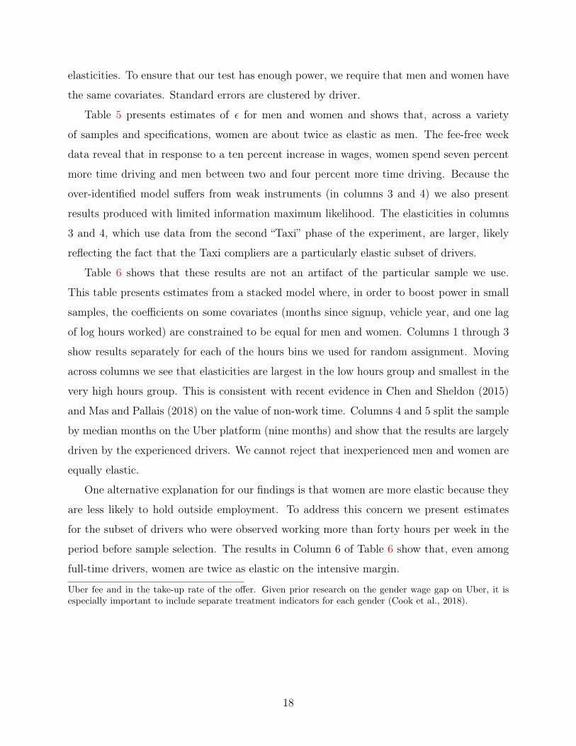
Table 5 presents estimates of ε for men and women and shows that, across a variety

of samples and specifications, women are about twice as elastic as men. The fee-free week

data reveal that in response to a ten percent increase in wages, women spend seven percent

more time driving and men between two and four percent more time driving. Because the

over-identified model suffers from weak instruments (in columns 3 and 4) we also present

results produced with limited information maximum likelihood. The elasticities in columns

3 and 4, which use data from the second “Taxi” phase of the experiment, are larger, likely

reflecting the fact that the Taxi compliers are a particularly elastic subset of drivers.

Table 6 shows that these results are not an artifact of the particular sample we use.

This table presents estimates from a stacked model where, in order to boost power in small

samples, the coefficients on some covariates (months since signup, vehicle year, and one lag

of log hours worked) are constrained to be equal for men and women. Columns 1 through 3

show results separately for each of the hours bins we used for random assignment. Moving

across columns we see that elasticities are largest in the low hours group and smallest in the

very high hours group. This is consistent with recent evidence in Chen and Sheldon (2015)

and Mas and Pallais (2018) on the value of non-work time. Columns 4 and 5 split the sample

by median months on the Uber platform (nine months) and show that the results are largely

driven by the experienced drivers. We cannot reject that inexperienced men and women are

equally elastic.

One alternative explanation for our findings is that women are more elastic because they

are less likely to hold outside employment. To address this concern we present estimates

for the subset of drivers who were observed working more than forty hours per week in the

period before sample selection. The results in Column 6 of Table 6 show that, even among

full-time drivers, women are twice as elastic on the intensive margin.

Uber fee and in the take-up rate of the offer. Given prior research on the gender wage gap on Uber, it isespecially important to include separate treatment indicators for each gender (Cook et al., 2018).

18

4.2 Extensive Margin Frisch Elasticities

We next turn to examining how drivers’ decision to drive in a given week responded to the

offer of higher wages. We present estimates of the reduced form equation

Driveit = ηFZit × Femalei + ηMZit ×Malei + βXit + εit (8)

where Xit includes dummies indicating the strata used for random assignment, driver gender,

the number of months a driver has been on the Uber platform, and indicators for whether a

driver uses Uber’s “vehicle solutions” leasing program. Driveit is an indicator for whether the

driver was active on the Uber platform that week. Zit indicates the percentage increase in

wages offered to the driver. This is clearly defined based on the structure of the experiment:

each driver is told what percentage increase in wages they will see if they opt in to the

treatment. For control drivers it is equal to zero. The sex-specific parameter η measures how

driver participation decisions respond to percentage changes in the offered wage. Standard

errors are clustered by driver.

To estimate these elasticities we use data from the first two weeks of the experiment,

which did not require drivers to make an up-front payment in order to get higher wages.

Because Taxi offers were only attractive to drivers who planned to drive at least a minimum

number of hours, it is unlikely that they had a large impact on whether drivers chose to

drive. Taxi offers have no impact on whether drivers choose to drive.

Table 7 shows that, across all groups, women are more responsive to the offer of higher

wages than men are. The results in column 1 reveal an average participation elasticity of

.12 for women and .04 for men: in response to a 10% increase in the offered wage, women

are 1.2 percentage points more likely to drive, compared with only 0.4 percentage points for

men. The next three columns break out the results by hours bin and show that the effects

are largest in the low hours group, which contains the drivers that are least attached to the

platform, and smallest in the very high hours group. The remaining columns divide drivers

by median months on platform (nine months) and by age. The results suggest that (1) less

experienced drivers are more responsive to the promotion and (2) there aren’t significant

differences between older and younger drivers.21

21The experienced and inexperienced groups each contain roughly equal numbers of drivers in the low, high,

19

The reduced form estimates do not correct for driver inattention. If drivers do not start

driving because they did not see the Earnings Accelerator offer, our estimates of η will be

biased downward. Panels B and C of Table 7 present two-stage least squares estimates of

Driveit = ηDit + βXit + εit (9)

Dit = γZit + λXit + υit, (10)

where Dit is an indicator for whether the driver accepted an Earnings Accelerator offer in

week t. The instrument in the just-identified model (Zit) is the same as before: the offered

percentage increase in wages. The over-identified model uses indicators for whether a driver

was offered fee-free driving interacted with week-of-offer and driver commission.

Column 1 of Table 7 shows that, once we scale by the participation rate, we obtain

extensive margin elasticities of .16 and .07 for women and men, respectively (Panel C).

These elasticities are significantly larger than the reduced form estimates in Table 7, but

still significantly smaller than most estimates in the literature.22 The estimated elasticities

are largest among low hours drivers—whose baseline participation rates are lowest—and

inexperienced or young drivers.

Interpretation Of course drivers participating in the Earnings Accelerator may differ

from those that did not participate. The econometric issue is that there are two types of

never-takers: (1) inelastic never-takers and (2) consent/inattention never-takers. Drivers in

the first group do not accept the offer because the offer is not generous enough to induce

them to drive; drivers in the second group do not accept the offer because they do not

want to participate in academic research or because they did not see the messaging. While

the two-stage least squares estimates identify the effect on compliers, the true extensive

margin elasticity combines the impact on compliers with the impact on inelastic never-

takers. Without information on the relative proportions of these two groups, it is impossible

for us to identify the true extensive margin elasticity. The reduced form and two-stage least

and very high bandwidths. This is largely because when we selected drivers for the experiment, we stratifiedon both commission and hours group. Drivers with a 20% commission are necessarily more experienceddrivers, because they had to join the platform before the commission changed.

22Chetty et al. (2013) report a mean extensive margin elasticity of .28 among the fifteen studies in theirmeta-analysis.

20

squares estimates give us lower and upper bounds, respectively.

The primary concern with interpreting our extensive margin results as extensive margin

Frisch elasticities is that drivers in our sample may hold second jobs in the non-gig economy.

However, this is not a concern for our analysis as long as long as the worker cannot adjust

their hours with less than a week’s notice. Our elasticities are within the range of recent

quasi-experimental results (Martinez, Saez and Siegenthaler, 2018). In general we expect

our results to be an upper-bound on the ‘true’ extensive margin elasticity since adjustment

costs are minimal in this setting.

5 Firm Substitution

We use data from repeated Earnings Accelerator experiments and a large-scale Uber pro-

motion to look at how drivers shift hours between platforms. Labor supply elasticities for

drivers that can work for multiple platforms (“shifters”) combine the market-level elasticities

we estimated in the previous section with firm-specific shifting. We use the formulas derived

in Section 2.2 to convert these elasticities into implied firm substitution elasticities.

5.1 Evidence from the Earnings Accelerator

We stack data from the three rounds of the Earnings Accelerator in order to identify firm- and

market-elasticities. The market labor supply elasticity—the increase in total hours worked

in response to a wage change—is identified by the responses of two groups: (1) Houston

drivers in the first Houston experiment and (2) Boston drivers that were ineligible for Lyft.

The opportunity to drive for other platforms makes drivers appear more elastic. Panel

A of Table 8 presents separate estimates of equation 6 for shifters and non-shifters. Column

1 shows that, on average, a non-shifter will increase hours worked by 8% in response to a

10% increase in hours. A shifter will increase hours by much more - 12.8% vs. 8%. The gap

between shifters and non-shifters is most pronounced among young drivers. This result is

consistent with younger drivers being more technologically adept, since more technologically

adept drivers find it easier to shift platforms.

Panel B breaks out the results by driver gender and shows that men and women respond

equally to the opportunity to multi-app. Column 1 shows that, across the three Earnings

21

Accelerator experiments, male drivers that cannot shift to competing platforms drive 6 per-

cent more when confronted with a 10% increase in hourly wages. However, male drivers

that can shift drive nearly 12 percent more. These additional hours likely come from Lyft,

and therefore do not reflect real increases in labor supply. Female drivers are generally more

responsive to increases in wages; both female shifters and non-shifters are more elastic than

their male counterparts. However, the gaps between shifters and non-shifters are roughly

the same size. The remaining columns of Table 8 show that the same pattern emerges across

different groups of drivers defined by experience and age.23

We can look for additional evidence of multi-apping by examining the utilization rates

(the fraction of the time a driver’s app is on that he/she is actively on a trip) of shifters

and non-shifters, and by looking at the impact of the treatment on utilization rates for each

group. Because drivers who multi-app spend less time waiting for dispatches, we should

see higher utilization rates among these drivers. Appendix Section B.2 presents additional

analysis showing that utilization rates are in fact higher among shifters. This is important

because only shifters can use multi-apping as a way to increase their earnings; non-shifters

can only work for Uber.

5.2 Evidence From Individual Driver Bonuses

Because our experimental elasticities in Section 5.1 are imprecise, we use data from a large-

scale Uber promotion we call the “Individual Driver Bonus” (IDB) program to corroborate our

findings. This promotion has two main advantages. First, unlike the Earnings Accelerator,

the data come from a single large city. Second, due to the structure of the promotion,

we are able to examine high earnings/hours drivers who we were unable to include in our

experiment. It is possible that a gender gap in shifting could emerge among these drivers.

As discussed in Section 3.3, drivers in this program were offered lump-sum payouts for

exceeding pre-specified trip thresholds. Figure A5 shows how the IDB incentive affects a

driver’s pay. The black line denotes the normal relationship between trips and total earnings.

The red line shows how this changes with the IDB incentive. A comparison of the solid and23Note that unlike in Section 4.1, we do not stratify by hours bin when examining shifting behavior.

Because our bandwidths are based on only Uber hours, drivers who can shift across platforms but have highhours on Uber, are less likely to be taking advantage of their option to shift.

22

dashed red lines reveals the difference between the low and high groups. The two groups

face the same earnings until the trip threshold, but there is a larger discontinuity in the high

group. The incentive structure is most attractive to drivers who, in the absence of treatment,

would be close to the trip threshold. For these drivers, the implied increase in wages due

to the incentive (the bonus spread across the additional trips they would need to complete)

is largest. Whether a driver completes more trips in response to the incentive depends on

three factors: (1) the size of the bonus, (2) the number of additional trips a driver needs to

take to cross the threshold, and (3) the curvature of the driver’s utility function.

Individuals that are offered the high bonuses are more likely to exceed the pre-specified

trip thresholds and complete more trips. Figure 3 plots kernel density estimates of trips

completed for drivers who faced a 40 trip threshold (indicated by a solid red line). While the

densities of both groups of drivers have a mass at exactly 40 trips, there is a larger spike for

drivers in the high group. Figure 4 plots similar kernel densities for the high group, splitting

drivers by sex and whether their car made them eligible for Lyft. The figure reveals that

there is a significantly larger spike among the male shifters than the male non-shifters. We

present similar, regression-based results, in Appendix Section B.3.

5.2.1 Estimation Strategy

We can derive estimates of drivers’ labor supply elasticities by assuming a parametric form

for trips completed without the incentive. Because all drivers face a fifty percent chance of

obtaining the high and low offer each period, there is no income effect. Use ti0 to denote

the number of trips driver i completes without the promotion and ti1 to denote the number

of trips driver i completes when given an offer. Individuals will receive the bonus if their

treated trips exceed the trip threshold. Use B to denote the lump sum bonus and T to

denote the trip threshold. Individuals will exceed the trip threshold if:

ti0 ≥ T (11)

ti0(1 + ε logB/T

w) ≥ T ti0 < T (12)

The first line simply states that, if a driver would have exceeded the threshold without

the incentive, they will with the incentive. The second line describes the conditions under

23

which a driver who would not have crossed the threshold without the incentive, crosses the

threshold with the incentive. This depends on the driver’s untreated trips (ti0), the amount

by which the incentive changes the wage (B/T )/w, and the labor supply elasticity (ε). A

larger trip elasticity leads more drivers to cross the trip threshold.24

We can estimate driver labor supply elasticities with or without assuming assumptions

about the distribution of trips completed. First, suppose trips are log-normally distributed

(perhaps conditional on some covariates). We can take logs of expression 11 and use the

approximation that log(1 + x) ≈ x for small x to re-write the expression as

log ti0 − ε log T + ε logB − ε logw ≥ log T

log ti0 ≥ −ε logB + ε logw + (1 + ε) log T

Assuming a mean of µ and a variance of σ2, the probability a driver exceeds the trip threshold

is

1− Φ

[− 1

σε logB +

1 + ε

σlog T +

1

σε logw − µ

σ

](13)

We can estimate this model using a probit where the dependent variable is whether a driver

crossed the trip threshold, B is the lump sum bonus and T is the trip threshold. The final

term is a function of average per-trip earnings. Because these may vary over time, we include

period fixed effects. We use the relationship between the coefficients on logB and log T to

estimate ε.

Figure A11 shows that the log-normal assumption is reasonable. First, we regress log

trips on date fixed effects and the hours bins from Table 4. Then, we plot the residuals,

along with a fitted normal curve. The figure on the left plots the residuals for the full

sample. The data roughly follow a normal distribution, but there is a spike to the right of

the mean. This is likely driven by bunching at the trip threshold. While the parametric

assumption applies to the control distribution (in the absence of IDB offers), we only observe

the treated distribution. Because the treatment is only likely to affect the distribution of

trips completed in a neighborhood of the trip threshold, we present a similar histogram,

omitting observations for drivers within a two-trip band of the trip threshold, in Panel B.

This distribution looks very similar to a normal distribution. The residual variance in the24Note that here the elasticity is in terms of trips, rather than hours.

24

four groups defined by sex and Lyft eligibility is nearly constant, ranging from .76 (male

non-shifters) to .81 (all other groups).

Alternatively, we can derive estimates of drivers’ labor supply elasticity without assuming

a parametric distribution for trips completed. Use pB,T to denote the fraction of drivers in

the treatment group and F0 to denote the distribution of trips for the control group. We can

re-write the opt-in equation as

F−10 [1− pB,T ] =T

1− εB/Tw

(14)

The left hand side of this equation is the quantile of the trip distribution corresponding to

the fraction of drivers in the high bonus group who exceeded the trip threshold. We estimate

equation 14 using non-linear least squares. See Appendix D.3 for a complete derivation and

for more details on the estimation.

5.2.2 IDB Elasticities

Table 10 presents labor supply elasticities for four different groups: (1) male non-shifters, (2)

male shifters, (3) female non-shifters, and (4) female shifters. We calculate these elasticities

using the structural relationship between the coefficients in the probit model described in

equation 13.25 The probit coefficients are reported in Appendix Table A8. The first two

columns present estimates from the baseline model in equation 11. The third and fourth

columns present results from a similar model where we re-weight the sample so that male

and female drivers are equally distributed across treatments.26 Because female drivers drive

fewer trips on average, they are more concentrated in ‘low’ treatment groups. Re-weighting

the sample allows us to account for the fact that drivers with different (untreated) driving

patterns may have different elasticities.

Our preferred specification is the instrumental variables specification presented in column

2. In response to a ten percent increase in wages, male drivers that cannot drive for com-25Each elasticity is calculated using the ratio of the coefficients on logB and log T . We use the fact that:βlogB

βlogB + βlog T=

−ε/σ−ε/σ + (1 + ε/)/σ

=−ε

−ε+ 1 + ε= −ε. Table 10 presents estimates of ε.

26For each group g we assign male drivers weights ofp(g|m)

p(g|f)where p(g|f) is the probability that a driver

is in group g, conditional on being female.

25

peting platforms increase their labor supply by ten percent; male drivers that can drive for

competing platforms increase their labor supply by almost fourteen percent. We expect these

additional hours came at the expense of Uber’s competitor, Lyft. We see a similar pattern

among women: female drivers that are limited to a single platform drive only eight percent

more in response to a ten percent wage increase, compared with nearly twelve percent. For

both male and female drivers, we reject the hypothesis that shifters and non-shifters have

the same elasticity. These results indicate that drivers shift between platforms in response

to changes in relative wages.

The theory described earlier says that firms have an incentive to pay lower wages to

workers who are less likely to leave for another firm. Prior, non-experimental, work has

suggested that women are less likely to leave. We find no evidence of that here. While

the male shifters are more elastic than the female shifters, the gap between shifters and

non-shifters is roughly equal for the two groups. In the next section we show that the firm

specific elasticities for men and women are statistically indistinguishable.

5.3 Firm Substitution Elasticities

We can use the the formulas in Section 2.3 to convert our labor supply elasticities into implied

firm substitution elasticities. We can also use these formulas to calculate the fraction of time

spend on other platforms.

We use data from the Earnings Accelerator experiments to estimate the fraction of time

male and female drivers spend on Uber, relative to ride-share as a whole. While these are not

firm-substitution elasticities, these provide information about how aggressively each group

optimizes their earnings. Because multi-apping is likely to always be a profitable strategy,

we should see lower fractions for men if they make more strategic labor supply decisions.

Table 9 presents the main results.

The first column estimates that men spend about half of their total ride-share/gig time

on Uber, though the standard errors can’t rule out relatively large fractions. Female drivers

appear to spend less total time on Uber, but the standard errors are again large and the

effects are insignificant. The experienced drivers appear to spend more time on competing

platforms, but, again, the results are imprecise.

With these fractions in hand, we compute firm-substitution elasticities using our IDB

26

estimates from the previous section and equation 4. These substitution elasticities measure

the extent to which drivers move hours onto Uber in response to changes in the Uber wage.

Column 1 of Table 12 shows estimated elasticities of between 2-4 for both male and

female drivers. These estimates are surprisingly similar to recent work by Dube, Manning

and Naidu (2017).27 We do not see any significant differences between male and female

drivers. If anything, women appear to be more elastic. The remaining columns show that

significant differences do not emerge in different subgroups. The fact that we do not see

gender differences in these firm-substitution elasticities indicates that gig economy firms

have little incentive to pay equally productive men and women different amounts.

6 Conclusion

We provided new evidence on the potential for gender differences in labor supply to explain

the gender wage gap. Firms with market power in the labor market have an incentive to pay

lower wages to workers who are less elastic to the firm: workers who are less willing to leave

in search of better wages elsewhere. We illustrated that once workers can choose their hours

freely, the optimal monopsonistic markdown depends on both the intensive margin elasticity

and on the firm substitution elasticity.

We then used experimentally induced variation to estimate intensive and extensive margin

Frisch elasticities for men and women. We found that women have Frisch elasticities roughly

double those of men. In response to a ten percent increase in wages, women are nearly two

percentage points more likely to drive at all, compared to one percentage point for men.

Conditional on driving, women drive eight percent more hours, compared to four percent

more for men. These elasticities—in particular the extensive margin elasticities—are modest

relative to those usually used to calibrate macro models.

We found that drivers shift hours between platforms (firms) when given the opportunity

to do so and that women are not significantly less likely to do so than men. To our knowledge,

we are the first to experimentally estimate separate firm-specific elasticities for men and

women. Taken as a whole, these results suggest that, at least in the gig economy, firms do27The authors use a bunching estimator to estimate firm-substitution elasticities from administrative wage

data and the CPS and from Amazon mTurk. Our estimates are larger than those reported for the online gigeconomy (mTurk) in that paper, but are very similar to those reported for the offline economy.

27

not have a strong incentive to wage discriminate between their male and female employees

(or independent contractors). To the extent that women may be particularly drawn to gig

economy employers due to a desire for flexible work arrangements, this is encouraging.

28

ReferencesAngrist, Joshua D., Sydnee Caldwell, and Jonathan V. Hall. 2017. “Uber Vs. Taxi:A Driver’s Eye View.” National Bureau of Economic Research Working Paper 23891.

Ashenfelter, Orley C, Henry Farber, and Michael R Ransom. 2010. “Labor MarketMonopsony.” Journal of Labor Economics, 28(2): 203–210.

Babcock, Linda, and Sara Laschever. 2009. Women Don’t Ask: Negotiation and theGender Divide. Princeton University Press.

Bhaskar, Venkataraman, Alan Manning, and Ted To. 2002. “Oligopsony andMonopsonistic Competition in Labor Markets.” The Journal of Economic Perspectives,16(2): 155–174.

Black, Dan A. 1995. “Discrimination in an Equilibrium Search Model.” Journal of LaborEconomics, 13(2): 309–334.

Boal, William M, and Michael R Ransom. 1997. “Monopsony in the Labor Market.”Journal of Economic Literature, 35(1): 86–112.

Card, David, Ana Rute Cardoso, Jörg Heining, and Patrick Kline. 2016. “Firmsand Labor Market Inequality: Evidence and Some Theory.” Journal of Labor Economics,53(1): S13–S70.

Card, David, Jörg Heining, and Patrick Kline. 2013. “Workplace Heterogeneity and theRise of West German Wage Inequality.” The Quarterly Journal of Economics, 128(3): 967–1015.

Chen, M Keith, and Michael Sheldon. 2015. “Dynamic Pricing in a Labor Market: SurgePricing and the Supply of Uber Driver-Partners.” University of California Los AngelesWorking Paper.

Chetty, Raj, Adam Guren, Day Manoli, and Andrea Weber. 2013. “Does indivisiblelabor explain the difference between micro and macro elasticities? A meta-analysis ofextensive margin elasticities.” NBER macroeconomics Annual, 27(1): 1–56.

Cook, Cody, Rebecca Diamond, Jonathan V. Hall, John A. List, and Paul Oyer.2018. “The Gender Earnings Gap in the Gig Economy: Evidence from over a Million UberDrivers.” Stanford University Working Paper.

Dube, Arindrajit, Alan Manning, and Suresh Naidu. 2017. “Monopsony and Em-ployer Mis-Optimization Account for Round Number Bunching in the Wage Distribution.”Working Paper.

Dube, Arindrajit, Jeff Jacobs, Suresh Naidu, and Siddharth Suri. forthcoming.“Monopsony in Online Labor Markets.” AER: Insights.

Farber, Henry S. 2005. “Is Tomorrow Another Day? the Labor Supply of New York CityCabdrivers.” Journal of Political Economy, 113(1): 46–82.

29

Farber, Henry S. 2015. “Why You Can’t Find a Taxi in the Rain and Other Labor SupplyLessons from Cab Drivers*.” The Quarterly Journal of Economics, 130(4): 1975–2026.

Fehr, Ernst, and Lorenz Goette. 2007. “Do Workers Work More If Wages Are High? Evi-dence from a Randomized Field Experiment.” The American Economic Review, 97(1): 298–317.

Hall, Jonathan V, and Alan B Krueger. 2015. “An Analysis of the Labor Market forUber’s Driver-Partners in the United States.” Princeton University Industrial RelationsSection Working Paper, 587.

Hall, Jonathan V, John J Horton, and Daniel T Knoepfle. 2017. “Labor MarketEquilibration: Evidence from Uber.” Working Paper, 1–42.

Hirsch, Boris, Thorsten Schank, and Claus Schnabel. 2010. “Differences in LaborSupply to Monopsonistic Firms and the Gender Pay Gap: An Empirical Analysis UsingLinked Employer-Employee Data from Germany.” Journal of Labor Economics, 28(2): 291–330.

Killingsworth, Mark R, and James J Heckman. 1986. “Female Labor Supply: ASurvey.” Handbook of Labor Economics, 1: 103–204.

King, Robert G, and Sergio T Rebelo. 1999. “Resuscitating real business cycles.” Hand-book of macroeconomics, 1: 927–1007.

Kline, Patrick, Neviana Petkova, Heidi Williams, and Owen Zidar. 2018. “WhoProfits from Patents? Rent-Sharing at Innovative Firms.” NBER Working Paper 25245.

Koustas, Dmitri. 2017. “Labor Supply and Consumption Insurance: Evidence fromRideshare Drivers.” University of California, Berkeley Working Paper.

Manning, Alan. 2003. Monopsony in Motion: Imperfect Competition in Labor Markets.Princeton University Press.

Manning, Alan. 2011. “Imperfect Competition in the Labor Market.” Handbook of LaborEconomics, 4: 973–1041.

Martinez, Isabel Z, Emmanuel Saez, and Michael Siegenthaler. 2018. “IntertemporalLabor Supply Substitution? Evidence from the Swiss Income Tax Holidays.” NationalBureau of Economic Research.

Mas, Alexandre, and Amanda Pallais. 2018. “Labor Supply and the Value of Non-WorkTime: Experimental Estimates from the Field.” American Economic Review: Insights.

McClelland, Robert, and Shannon Mok. 2012. “A Review of Recent Research on LaborSupply Elasticities.”

Oettinger, Gerald S. 1999. “An Empirical Analysis of the Daily Labor Supply of StadiumVendors.” Journal of political Economy, 107(2): 360–392.

30

Ransom, Michael R, and Ronald L Oaxaca. 2010. “New Market Power Models andSex Differences in Pay.” Journal of Labor Economics, 28(2): 267–289.

Robinson, Joan. 1933. The Economics of Imperfect Competition. Palgrave Macmillan.

Stafford, Tess M. 2015. “What Do Fishermen Tell Us That Taxi Drivers Do Not? anEmpirical Investigation of Labor Supply.” Journal of Labor Economics, 33(3): 683–710.

Tirole, Jean. 1988. The Theory of Industrial Organization. MIT press.

Webber, Douglas A. 2016. “Firm-Level Monopsony and the Gender Pay Gap.” IndustrialRelations: A Journal of Economy and Society, 55(2): 323–345.

31

7 Figures and Tables

Figure 1: Multi-Apping Discussion on UberPeople

Note: The above picture is a screenshot from “Uber People”, an online forum and discussion boardwhere drivers discuss ride-share related topics. The forum is not affiliated with Uber Technologies,Inc. or any other ride-share company. The conversation highlights that drivers are interested inmulti-apping but find it requires a non-trivial amount of effort.

32

Figure 2: Example of a Third Party Multi-Apping Application

Note: This is a screenshot of a TechCrunch article discussing a third party app, Mystro, whichhelps drivers quickly switch between competing ride-share platforms.

33

Figure 3: Example of Bunching Around IDB Threshold

0.0

2.0

4.0

6De

nsity

0 20 40 60 80 100Number of Trips

Low Offer High Offer

Note: This figure plots Gaussian kernel density estimates of the distribution of trips completed fordrivers in the high and low bonus groups with a 40 trip threshold using a bandwidth of 2. Weselected this trip threshold because it contains the largest number of female non-shifters (and thesecond largest number of drivers overall). The dashed red lines denote additional trip thresholds.Drivers were offered up to two incentives per period.

34

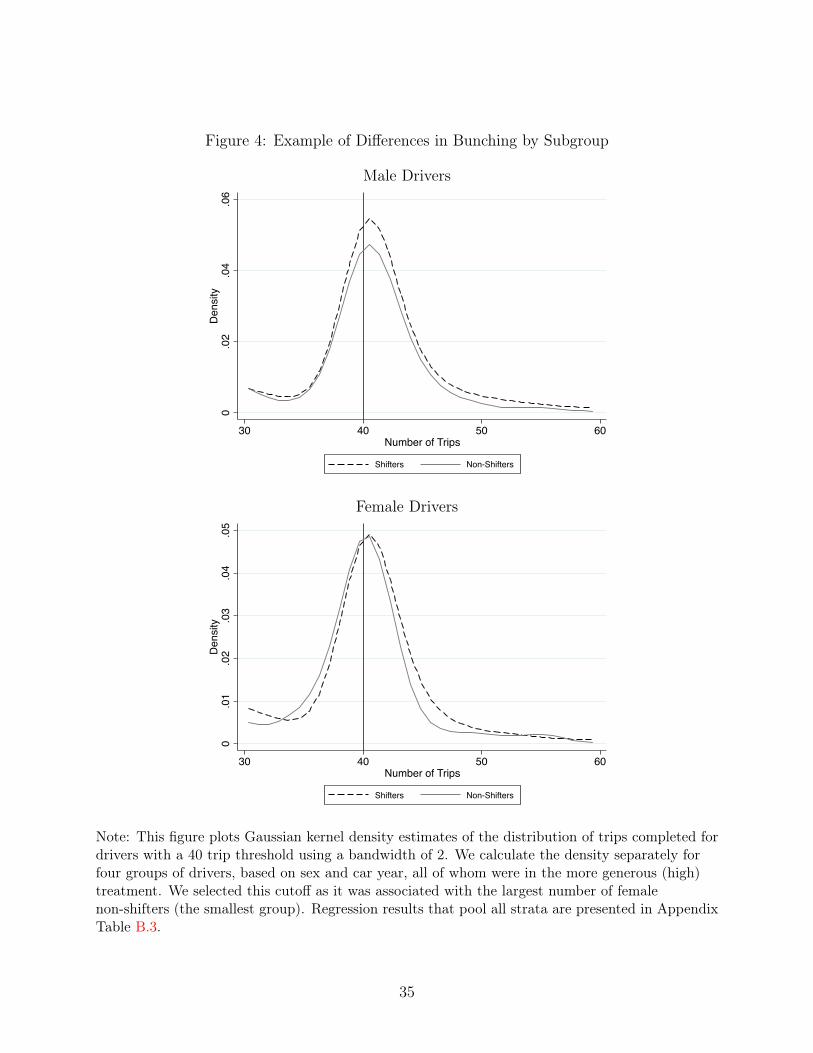
Figure 4: Example of Differences in Bunching by Subgroup

Male Drivers

0.0

2.0

4.0

6D

ensi

ty

30 40 50 60Number of Trips

Shifters Non-Shifters

Female Drivers

0.0

1.0

2.0

3.0

4.0

5D

ensi

ty

30 40 50 60Number of Trips

Shifters Non-Shifters

Note: This figure plots Gaussian kernel density estimates of the distribution of trips completed fordrivers with a 40 trip threshold using a bandwidth of 2. We calculate the density separately forfour groups of drivers, based on sex and car year, all of whom were in the more generous (high)treatment. We selected this cutoff as it was associated with the largest number of femalenon-shifters (the smallest group). Regression results that pool all strata are presented in AppendixTable B.3.

35

Table 1: Timeline

City WeekBeginning ActionBoston August15,2016 SampleselectionforBostonexperiment

August22,2016 Wave1NotificationsandOpt-InAugust29,2016 Wave1Opt-InsDriveFeeFree;Wave2NotificationsandOpt-InSeptember5,2016 Wave2Opt-InsDriveFeeFreeSeptember12,2016 Taxi1OffersandOpt-InSeptember19,2016 Taxi1LiveSeptember26,2016October3,2016October10,2016 Taxi2OffersandOpt-InOctober17,2016 Taxi2Live

Houston March27,2017 Sampleselectionforround1ofHoustonApril3,2017 Wave1NotificationsandOpt-InApril10,2017 Wave1Opt-InsDriveFee-Free;Wave2NotificationsandOpt-InApril17,2017 Wave2Opt-InsDriveFee-FreeApril24,2017May1,2017 Taxi1OffersandOpt-InMay8,2017 Taxi1LiveMay15,2017 Taxi2OffersandOpt-InMay22,2017 Taxi2LiveMay29,2017 LyftEntersHouston

September11,2017 Sampleselectionforround2ofHoustonSeptember18,2017 Wave1NotificationsandOpt-InSeptember25,2017 Wave1Opt-InsDriveFee-Free;Wave2NotificationsandOpt-InOctober2,2017 Wave2Opt-InsDriveFee-FreeOctober9,2017October16,2017 Taxi1OffersandOpt-InOctober23,2017 Taxi1Live

Note: This table presents the timeline of the three Earnings Accelerator experiments. Eachexperiment unfolded in three stages. First, we defined the eligible sample, based on drivers’ tripsand hours over the prior four weeks and randomly selected a subset of drivers to participate in theexperiment. We picked half of the drivers to receive the offer of fee-free driving in one week (wave1); the second half received offers the following week (wave 2). Finally, we offered random subsetsof drivers who opted in to fee-free driving the opportunity to buy additional weeks of fee-free orreduced-fee driving, for an upfront payment. We conducted two weeks of Taxi treatments inBoston and in the first Houston experiment. We were only able to conduct one week in the secondHouston experiment, as a result of changes in the Uber app.

36

Table 2: Sample Counts

Boston Houston1 Houston2

IndividualDriverBonus

(1) (2) (3) (4)MaleDrivers 1431 972 1283 48527Shifters 230 0 1283 47958Non-Shifters 1201 972 0 569

FemaleDrivers 232 1048 817 10923Shifters 28 0 817 10794Non-Shifters 204 1048 0 129

Note: This table gives the sample counts of male and female drivers in the three Earnings Acceleratorexperiments and in the IDB sample. We call drivers who could drive for Lyft shifters, and thosecould not non-shifters. Boston drivers are considered non-shifters if they have a car model year 2003or older. No drivers in Houston 1 are considered shifters because Lyft was not present in the marketat that time. All drivers in Houston 2 are considered shifters because Lyft had already re-enteredthe market. IDB drivers are considered shifters if their car model year is 2003 or older.

37

Table 3: Characteristics of Male and Female Drivers

Male Female Male Female Male Female Male Female(1) (2) (3) (4) (5) (6) (5) (6)

Age 42.8 43.6 44.0 44.3 41.8 42.6 41.0 40.3(12.5) (11.9) (12.5) (11.9) (13.6) (13.6) (12.0) (11.9)[42.0] [43.0] [43.0] [44.0] [40.0] [42.2] [39.3] [38.9]

MonthsonPlatform 14.2 8.1 20.1 12.2 10.5 8.6 17.5 12.1(10.1) (8.5) (9.5) (9.3) (8.9) (7.4) (13.7) (10.9)[12.0] [4.2] [21.5] [9.3] [8.5] [6.4] [14.3] [9.4]

TripsCompleted 1413.3 581.6 1707.3 861.21653.4 893.4 1820.3 1111.2797.0 250.0 1047.0 474.0

VehicleSolutions 0.1 0.1 0.1 0.1 0.0 0.0 0.0 0.0(0.3) (0.3) (0.3) (0.4) (0.0) (0.0) (0.0) (0.0)[0] [0] [0] [0] [0] [0] [0] [0]

ModelYear 2012.4 2013.3 2013.4 2013.7 2002.6 2002.6 2013.7 2013.7(3.8) (3.0) (2.5) (2.5) (0.6) (0.5) (3.2) (3.1)

[2013.0] [2014.0] [2014.0] [2014.0] [2003.0] [2003.0] [2015.0] [2015.0]AverageHours/Week 19.4 18.0 20.7 18.6 9.5 7.7 12.3 8.9

(12.1) (11.7) (14.5) (12.7) (6.3) (4.3) (8.3) (6.9)[17.0] [15.6] [17.7] [16.0] [8.6] [7.0] [10.6] [7.5]

Observations 3623 2097 972 1048 569 129 47958 10794

Non-Shifters ShiftersFullSample Houston1EarningsAccelerator IndividualDriverBonus

Note: This table includes all experimental drivers and IDB drivers included in our analysis. The first two columns compare male andfemale drivers included in any of the three Earnings Accelerator experiments. The third and fourth columns compare male and femaledrivers in the first Houston experiment (pre-Lyft). These are the drivers included in the analysis in Section 4. The remaining fourcolumns compare male and female drivers in the Individual Driver Bonus sample.

38

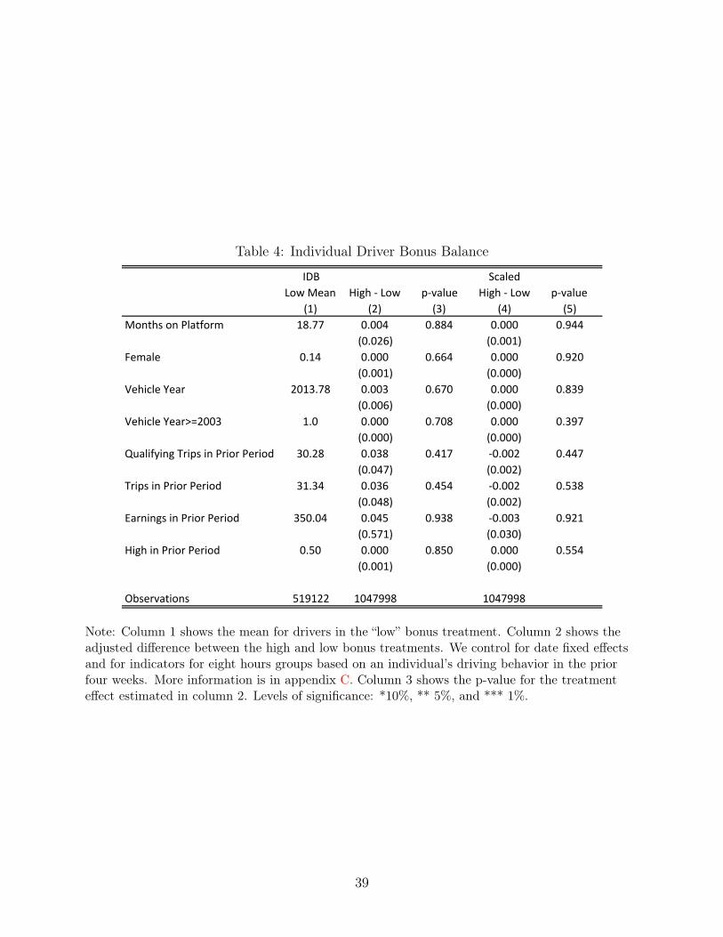
Table 4: Individual Driver Bonus Balance

IDB Scaled

LowMean High-Low p-value High-Low p-value

(1) (2) (3) (4) (5)

MonthsonPlatform 18.77 0.004 0.884 0.000 0.944

(0.026) (0.001)

Female 0.14 0.000 0.664 0.000 0.920

(0.001) (0.000)

VehicleYear 2013.78 0.003 0.670 0.000 0.839

(0.006) (0.000)

VehicleYear>=2003 1.0 0.000 0.708 0.000 0.397

(0.000) (0.000)

QualifyingTripsinPriorPeriod 30.28 0.038 0.417 -0.002 0.447

(0.047) (0.002)

TripsinPriorPeriod 31.34 0.036 0.454 -0.002 0.538

(0.048) (0.002)

EarningsinPriorPeriod 350.04 0.045 0.938 -0.003 0.921

(0.571) (0.030)

HighinPriorPeriod 0.50 0.000 0.850 0.000 0.554

(0.001) (0.000)

Observations 519122 1047998 1047998

Note: Column 1 shows the mean for drivers in the “low” bonus treatment. Column 2 shows theadjusted difference between the high and low bonus treatments. We control for date fixed effectsand for indicators for eight hours groups based on an individual’s driving behavior in the priorfour weeks. More information is in appendix C. Column 3 shows the p-value for the treatmenteffect estimated in column 2. Levels of significance: *10%, ** 5%, and *** 1%.

39

Table 5: Frisch Elasticities

Male Female Male Female Male Female(1) (2) (3) (4) (5) (6)

LogWages 0.43* 0.75*** 0.61** 1.31*** 0.52*** 1.00***(0.23) (0.16) (0.26) (0.24) (0.18) (0.14)

LogWages 0.22 0.69*** 0.64** 1.10*** 0.44** 0.90***(0.23) (0.16) (0.27) (0.22) (0.18) (0.14)

FirstStageFStatistic 13.4 14.6 6.5 7.5 10.5 11.2p-valuefromtestofequality

LogWages 0.26 0.73*** 0.71** 1.17*** 0.53** 0.97***(0.30) (0.17) (0.30) (0.24) (0.22) (0.15)

p-valuefromtestofequality

Drivers 714 766 479 565 752 805Observations 1341 1425 868 1016 2209 2441

0.045 0.062 0.015

0.042 0.051 0.012

C.LIML

FreeWeek Taxi Stacked

A.Just-Identified2SLS

B.Over-Identified2SLS

Note: All models control for the strata used for random assignment, date fixed effects, the numberof months a driver has been on the platform, whether a driver uses the "vehicle solutions"program, and one lag of log earnings. We also include a dummy variable for whether the driverdrove at all in the prior week; for drivers that did not drive, we recode their lag earnings to 0. Thep-values for the 2SLS and LIML models come from stacked models where the coefficient on eachcovariate is restricted to be equal for men and women. The over-identified model includes 12binary instruments for free week and 12 binary instruments for Taxi. Within each treatment typethere is a binary instrument for each combination of: commission group (2), treatment week (2),and hours group (3). Table A7 presents analogous results without baseline covariates. Standarderrors are clustered by driver. Levels of significance: *10%, ** 5%, and *** 1%.

40

Table 6: Frisch Elasticities by Subgroup

Low High VeryHigh Experienced Inexperienced 35orYounger

Olderthan

35 40+Hours

Weekday

Afternoon

NoLate

Nights

(1) (2) (3) (4) (5) (6) (7) (8) (9) (10)

LogWages*Male 0.44 0.42** 0.33 0.27 0.37 0.39* 0.75** 0.35 0.30 0.40

(0.29) (0.20) (0.25) (0.18) (0.27) (0.20) (0.32) (0.24) (0.20) (0.32)

LogWages*Female 1.11*** 0.77*** 1.10*** 1.14*** 0.56** 0.98*** 0.77*** 0.79*** 0.73*** 0.66***

(0.26) (0.15) (0.27) (0.20) (0.26) (0.15) (0.17) (0.25) (0.15) (0.21)

p-valueforequality 0.069 0.146 0.030 0.001 0.590 0.014 0.941 0.187 0.072 0.463

Drivers 406 1151 604 1018 414 1140 539 414 843 478

Observations 1115 3535 1938 3062 1182 3458 1588 1337 2766 1303

DOFILE:frisch.do

UsualHoursByHoursGroup ByMonthsonPlatform ByAge

Note: Columns 1-3 stratify by the hours groups used for random assignment. Columns 4 and 5 present results for experienced drivers(those who have been on the platform for more than 9 months) and inexperienced drivers. Columns 6-7 split the sample by driver age.Columns 8-10 present estimates for different subgroups, based on usual (non-treatment week) hours worked. Column 8 includes alldrivers who worked more than 40 hours in at least one of the four weeks we used for sample selection. Column 9 includes drivers who,during the course of the experiment, were observed working for at least ten minutes between 3 p.m. and 7 p.m. on at least ten distinctweek-days (out of forty maximum in our sample). Column 10 includes drivers that never work after 11 P.M. or before 4 A.M. All modelscontrol for the strata used for random assignment, date fixed effects, the number of months a driver has been on the platform, whether adriver uses the "vehicle solutions" program, and one lag of log earnings. We also include a dummy variable for whether the driver droveat all in the prior week; for drivers who did not drive, we recode their lag of earnings to 0. The p-value comes from a stacked modelwhere the coefficients on each covariate is restricted to be equal for men and women. The over-identified models include 24 binaryinstruments for each gender; these reflect the 4 treatment weeks, 3 hours groups, and 2 commission groups. Standard errors areclustered by driver. Levels of significance: *10%, ** 5%, and *** 1%.

41

Table 7: Extensive Margin Elasticities

All Low High VeryHigh Experienced Inexperienced35or

YoungerOlderthan

35(1) (2) (3) (4) (5) (6) (7) (8)

Male 0.04 0.04 0.05 0.00 0.01 0.12* -0.01 0.06(0.03) (0.06) (0.04) (0.04) (0.04) (0.07) (0.06) (0.04)

Female 0.12*** 0.20*** 0.08** -0.05 0.09* 0.14*** 0.13** 0.12***(0.03) (0.07) (0.04) (0.04) (0.05) (0.04) (0.07) (0.04)

p-value 0.10 0.07 0.48 0.40 0.19 0.83 0.10 0.35

Male 0.09 0.05 0.11* -0.01 0.05 0.20* 0.02 0.11(0.06) (0.11) (0.07) (0.07) (0.07) (0.11) (0.10) (0.07)

Female 0.18*** 0.32*** 0.12** -0.05 0.15** 0.20*** 0.20* 0.17***(0.04) (0.10) (0.05) (0.06) (0.06) (0.06) (0.10) (0.05)

p-value 0.23 0.07 0.93 0.68 0.30 0.98 0.22 0.50

Male 0.06 0.06 0.07 0.00 0.02 0.23** 0.00 0.10(0.06) (0.11) (0.06) (0.07) (0.06) (0.11) (0.10) (0.07)

Female 0.16*** 0.31*** 0.11** -0.06 0.13** 0.19*** 0.22** 0.15***(0.04) (0.10) (0.05) (0.05) (0.06) (0.06) (0.10) (0.05)

p-value 0.15 0.09 0.61 0.53 0.21 0.77 0.12 0.51

Observations 4040 1334 2706 1352 2566 1474 1186 2860

ByAge

B.Just-Identified2SLS

A.ReducedForm

C.Over-Identified2SLS

ByHoursGroup ByMonthsonPlatform

Note: This table presents estimates of the extensive margin labor supply elasticity estimated based on models in equation 8 and 9. Allmodels control for the strata used for random assignment, date fixed effects, the number of months a driver has been on the platform,whether a driver uses the "vehicle solutions" program, and driver gender. The over-identified model includes 12 binary instruments foreach gender, one for each combination of: commission group (2), treatment week (2), and hours group (3). The just-identified modelincludes a single treatment indicator for each gender. Standard errors are clustered by driver. Levels of significance: *10%, ** 5%, and*** 1%.

42

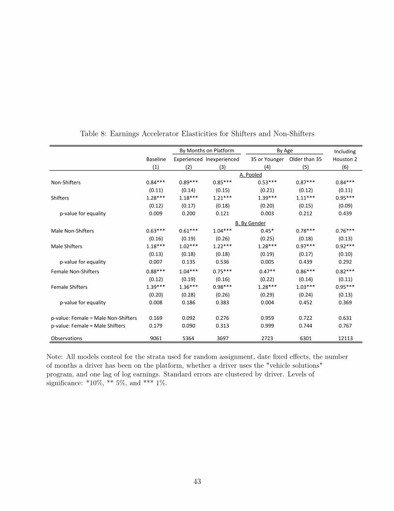
Table 8: Earnings Accelerator Elasticities for Shifters and Non-Shifters

Baseline Experienced Inexperienced 35orYounger Olderthan35(1) (2) (3) (4) (5) (6)

Non-Shifters 0.84*** 0.89*** 0.85*** 0.53*** 0.87*** 0.84***(0.11) (0.14) (0.15) (0.21) (0.12) (0.11)

Shifters 1.28*** 1.18*** 1.21*** 1.39*** 1.11*** 0.95***(0.12) (0.17) (0.18) (0.20) (0.15) (0.09)

p-valueforequality 0.009 0.200 0.121 0.003 0.212 0.439

MaleNon-Shifters 0.63*** 0.61*** 1.04*** 0.45* 0.78*** 0.76***(0.16) (0.19) (0.26) (0.25) (0.18) (0.13)

MaleShifters 1.18*** 1.02*** 1.22*** 1.28*** 0.97*** 0.92***(0.13) (0.18) (0.18) (0.19) (0.17) (0.10)

p-valueforequality 0.007 0.135 0.536 0.005 0.439 0.292

FemaleNon-Shifters 0.88*** 1.04*** 0.75*** 0.47** 0.86*** 0.82***(0.12) (0.19) (0.16) (0.22) (0.14) (0.11)

FemaleShifters 1.39*** 1.36*** 0.98*** 1.28*** 1.03*** 0.95***(0.20) (0.28) (0.26) (0.29) (0.24) (0.13)

p-valueforequality 0.008 0.186 0.383 0.004 0.452 0.369

p-value:Female=MaleNon-Shifters 0.169 0.092 0.276 0.959 0.722 0.631p-value:Female=MaleShifters 0.179 0.090 0.313 0.999 0.744 0.767

Observations 9061 5364 3697 2723 6301 12113

B.ByGender

A.Pooled

ByMonthsonPlatform ByAge IncludingHouston2

Note: All models control for the strata used for random assignment, date fixed effects, the numberof months a driver has been on the platform, whether a driver uses the "vehicle solutions"program, and one lag of log earnings. Standard errors are clustered by driver. Levels ofsignificance: *10%, ** 5%, and *** 1%.

43

Table 9: Estimates of the Fraction of Ride-Share Time Spent on Uber

Baseline Experienced Inexperienced(1) (2) (3)

MaleDrivers 0.54*** 0.61*** 0.86***(0.15) (0.22) (0.22)

FemaleDrivers 0.64*** 0.76*** 0.76***(0.10) (0.14) (0.22)

p-valueforequality 0.20 0.15 0.19

Observations 9061 5364 3697

ByMonthsonPlatform

Note: This table uses the elasticities in Table 8 to estimate φ using the formula in equation 5. Allmodels control for the strata used for random assignment, date fixed effects, the number ofmonths a driver has been on the platform, whether a driver uses the "vehicle solutions" program,and one lag of log earnings. Standard errors are clustered by driver. Levels of significance: *10%,** 5%, and *** 1%.

44

Table 10: Individual Driver Bonuses: Elasticities

Probit IV-Probit Probit IV-Probit(1) (2) (3) (4) (5)

MaleNon-Shifters 0.881*** 1.080*** 0.894*** 1.184*** 1.143***(0.014) (0.035) (0.016) (0.041) (0.214)

MaleShifters 1.357*** 1.367*** 1.379*** 1.358*** 1.564***(0.008) (0.008) (0.010) (0.010) (0.027)

p-value:MaleShifters=Non-Shifters 0.000 0.124 0.000 0.386 0.050

FemaleNon-Shifters 0.708*** 0.821*** 0.672*** 0.824*** 1.509***(0.052) (0.102) (0.051) (0.102) (0.302)

FemaleShifters 1.163*** 1.183*** 1.185*** 1.225*** 1.176***(0.005) (0.006) (0.006) (0.008) (0.053)

p-value:FemaleShifters=Non-Shifters 0.049 0.263 0.027 0.217 0.284

p-value:Female=MaleNon-Shifters 0.494 0.479 0.382 0.335 0.336p-value:Female=MaleShifters 0.000 0.006 0.000 0.066 0.000

Observations 1047998 1047998 1047998 1047998 1047994

ParametricUnweighted Weighted Non-

Parametric

Note: This table presents elasticities for male and female non-shifters, estimated using data fromthe IDB program. The parametric and non-parametric models are discussed in Section 5.2 in thetext and in Appendix Section D.3. The standard errors for the parametric model are clustered bydriver. Observations in columns 3 and 4 are re-weighted so that male drivers have the samedistribution across treatment groups as female drivers. The IV-probit model uses treatment (highbonus) indicators, interacted with gender and “shift” status as instruments for the size of thebonus the driver was offered. Appendix Table A8 presents the raw probit coefficients. Thestandard errors in column 5 are computed using 500 bootstrap replications. Levels of significance:*10%, ** 5%, and *** 1%.

45

Table 11: Individual Driver Bonuses: Elasticities by Subgroup

VeryHigh Low

Younger

than35

Olderthan

35

Above

Median

Below

Median

(1) (2) (3) (4) (5) (6)

MaleNon-Shifters 0.390*** 1.626*** 1.865*** 1.217*** 1.452*** 1.421***

(0.146) (0.420) (0.537) (0.314) (0.413) (0.381)

MaleShifters 0.571*** 1.869*** 1.873*** 1.656*** 1.648*** 1.701***

(0.073) (0.421) (0.396) (0.255) (0.250) (0.323)

p-value:MaleShifters=Non-Shifters 0.206 0.565 0.987 0.175 0.623 0.453

FemaleNon-Shifters 0.366 1.05** 0.96** 0.802 1.168 0.89**

(0.412) (0.483) (0.415) (0.510) (1.550) (0.377)

FemaleShifters 0.498*** 1.620*** 1.429*** 1.364*** 1.268*** 1.549***

(0.061) (0.303) (0.248) (0.169) (0.162) (0.246)

p-value:FemaleShifters=Non-Shifters 0.715 0.222 0.338 0.212 0.930 0.103

p-value:Female=MaleNon-Shifters 0.957 0.332 0.163 0.478 0.859 0.294

p-value:Female=MaleShifters 0.099 0.174 0.042 0.040 0.013 0.330

Observations 437622 610376 346945 701053 525201 522797

ByTripGroup ByAge ByExperience

Note: This table presents elasticity estimates based on the parametric model discussed in Section 5.2. The elasticities come from aprobit model where we instrument the size of the offered bonus with treatment indicators, interacted with gender and and indicator forwhether the driver is a “shifter”. Standard errors are clustered by driver. Levels of significance: *10%, ** 5%, and *** 1%.

46

Table 12: Firm-Specific Elasticities

AllDrivers

Above

Median

Below

Median

35or

Younger

Olderthan

35

(1) (2) (3) (4) (5)

Male 2.736 0.096 3.477 3.477 1.842

(2.647) (3.497) (3.264) (3.264) (3.673)

Female 3.983 4.178 5.023 5.023 5.892

(4.602) (5.317) (6.064) (6.064) (4.743)

p-valueforequality 0.813 0.516 0.822 0.822 0.494

Observations 1047998 437622 610376 346945 701053

ByAgeByExperience

Note: This table uses the formulas in Section 2.3 to translate the elasticities presented in Table 10into implied firm-specific elasticities. Levels of significance: *10%, ** 5%, and *** 1%.

47

A Appendix Tables and Figures

Figure A1: Multi-Apping

Note: This is a screenshot from rideshareapps.com’s guide on how to drive for Lyft and Uber atthe same time. This is intended to illustrate that multiple non-Uber/Lyft affiliated forums provideinformation to drivers on how to maximize earnings via multi-apping.

48

Figure A2: Earnings Accelerator Messaging

8/22/2016 Uber Mail - Fwd: Opt in for fee-free driving!

https://mail.google.com/mail/u/0/?ui=2&ik=1fb4a73203&view=pt&search=inbox&msg=156b25dcdcdc0da8&siml=156b25dcdcdc0da8 1/2

FEE-less in the summer!

To celebrate summer rides, we are launching a special driver-partnerpromotion — the Earnings Accelerator! To claim this offer, click the buttonbelow by Saturday, August 27 at 11:59pm, and you’ll keep the Uber fee onevery ride between August 29 and September 5.

Emily Oehlsen <eo@uber.com>

Fwd: Opt in for fee­free driving!

Josh Angrist <angrist@mit.edu> Mon, Aug 22, 2016 at 6:08 AMTo: Emily Oehlsen <eo@uber.com>, Sydnee Caldwell <sydneec@mit.edu>

accelerator email

­­­­­­­­ Forwarded Message ­­­­­­­­Subject:Opt in for fee­free driving!

Date:Mon, 22 Aug 2016 07:00:45 ­0600From:Uber <email@et.uber.com>

Reply­To:Uber <reply­fe8d10737062067470­351_HTML­6762658­6350024­1@et.uber.com>To:angrist@mit.edu

 

Note: This figure shows the e-mails and text messages that were sent to drivers selected for theEarnings Accelerator. The link in the text message and the link in the email (not included in thepicture) directed the driver to a more detailed opt-in page with information on how the incentiveworked and with consent language. This opt-in form is depicted in Figure A3.

49

Figure A3: Earnings Accelerator Opt-In Form

Note: This is a screenshot from the opt-in form sent to drivers included in the first EarningsAccelerator experiment (in Boston). Drivers were sent to this page via the in-app notification andvia text messages and e-mails they received throughout opt-in week. The form pre-filled with theirunique Uber identifier (not included in screenshot). To opt in, the driver only needed to scroll tothe bottom of the page and click submit.

50

Figure A4: Sample Weekly Pay Statement

8/26/16, 5:19 PMPay Statements

Page 1 of 2https://partners.uber.com/p3/money/statements/index

Partner Earnings

!

TOTAL EARNINGS

$19.34

3COMPLETED TRIPS

0h 55mONLINE HOURS

100%ACCEPTANCE RATE

0DRIVER CANCELLATIONS

3COMPLETED TRIPS

0h 55mONLINE HOURS

100%

PAY PERIOD

Current Statement

PAY PERIOD

Current Statement

▾▾

8/26/16, 5:19 PMPay Statements

Page 2 of 2https://partners.uber.com/p3/money/statements/index

100%ACCEPTANCE RATE

0DRIVER CANCELLATIONS

Weekly Earnings

Estimated Payout $19.34

Trip Earnings $19.34

Fare $24.12

Uber Fee - $6.03

Toll + $1.25

"

Note: This figure shows that, when we ran the experiment, drivers’ weekly pay statements listed(1) how much they collected in trip receipts, (2) how much of this went to Uber in the form of theUber fee, and (3) what, if any, reimbursements they received for tolls. Their estimated payout wasthe sum of these three items. The structure of drivers’ weekly earning statements has changedsince we ran the experiment.

51

Figure A5: Individual Driver Bonus: Budget Set

Note: This figure shows a stylized budget set for the IDB incentive studied in Section 5.2 of thispaper. The x-axis denotes trips and the y-axis denotes total take-home earnings. For a given tripthreshold X, drivers in the IDB were told that they would receive a lump-sum bonus for exceedingthe trip threshold. The amount of the bonus and the trip threshold varied across drivers and weeks.The blue curve shows a utility curve of a driver who, in the absence of the incentive would notexceed the trip threshold. The budget set for the high bonus cuts through her indifference curve,though the budget set for the low bonus does not. Therefore this driver will only exceed the tripthreshold (labeled X) if offered the high bonus.

52

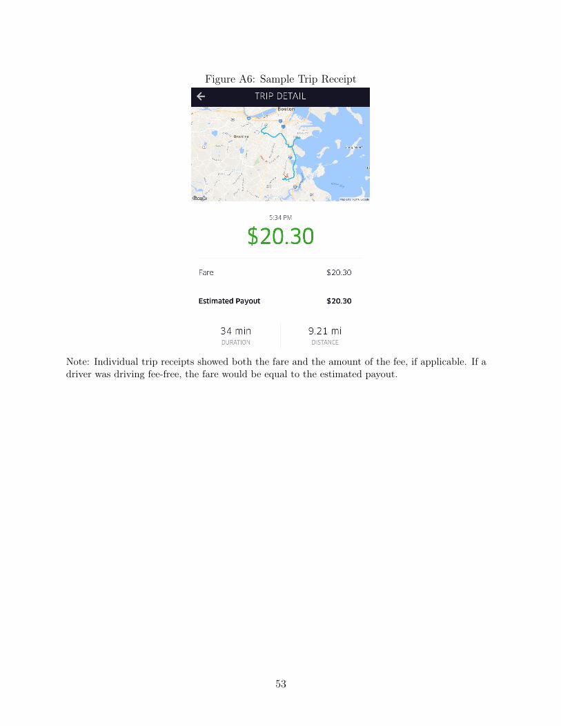
Figure A6: Sample Trip Receipt

Note: Individual trip receipts showed both the fare and the amount of the fee, if applicable. If adriver was driving fee-free, the fare would be equal to the estimated payout.

53

Figure A8: Earnings Accelerator Buy-In

Note: This shows a sample trip receipt of a driver who accepted one of the Taxi offers. The leaseamount is broken out from the trip receipts, and is identified as a promotional payment. This isnot a screenshot from a driver in our experiment; we did not offer leases that cost $220.

Figure A7: Earnings Accelerator Lease Calculator

Note: Each driver who was offered a Taxi offer was sent a slider that allowed them to compare theearnings they would receive if they accepted the offer (net of the lease) to the earnings they wouldnormally receive. The slider was set to load at the breakeven (the place where treated anduntreated earnings would be identical).

54

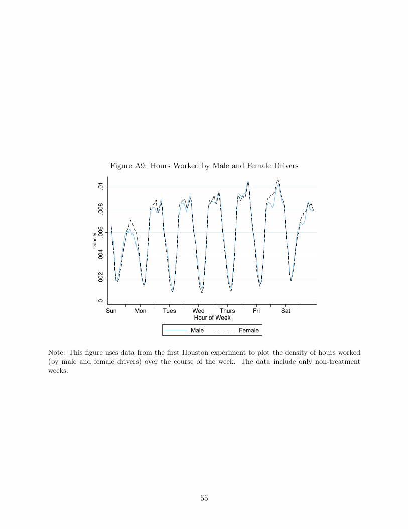
Figure A9: Hours Worked by Male and Female Drivers

0.0

02.0

04.0

06.0

08.0

1D

ensi

ty

Sun Mon Tues Wed Thurs Fri Sat Hour of Week

Male Female

Note: This figure uses data from the first Houston experiment to plot the density of hours worked(by male and female drivers) over the course of the week. The data include only non-treatmentweeks.

55

Figure A10: Age and Experience Distributions by Subgroup: IDB SamplePanel A: Age

0.0

1.0

2.0

3Ag

e

20 40 60 80Kernel Density

Male Female

0.0

1.0

2.0

3Ag

e

20 40 60 80Kernel Density

Non-Shifter Shifter

Panel B: Months on Platform

0.0

2.0

4.0

6Ex

perie

nce

0 20 40 60 80Kernel Density

Male Female

0.0

2.0

4.0

6Ex

perie

nce

0 10 20 30 40Kernel Density

Non-Shifter Shifter

Note: This figure presents kernel densities of driver age and experience (months on platform) in the IDB sample.

56

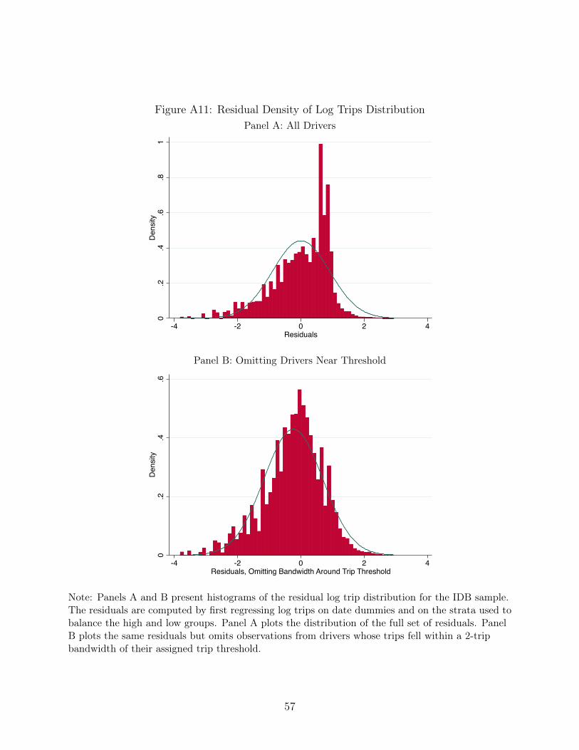
Figure A11: Residual Density of Log Trips DistributionPanel A: All Drivers

0.2

.4.6

.81

Density

-4 -2 0 2 4Residuals

Panel B: Omitting Drivers Near Threshold

0.2

.4.6

Dens

ity

-4 -2 0 2 4Residuals, Omitting Bandwidth Around Trip Threshold

Note: Panels A and B present histograms of the residual log trip distribution for the IDB sample.The residuals are computed by first regressing log trips on date dummies and on the strata used tobalance the high and low groups. Panel A plots the distribution of the full set of residuals. PanelB plots the same residuals but omits observations from drivers whose trips fell within a 2-tripbandwidth of their assigned trip threshold.

57

Table A1: Earnings Accelerator Balance: Boston

Week1- TaxiWeek1 TaxiWeek2Eligible Experimental Week2 Treated-Control Treated-ControlDrivers Difference Difference Difference Difference(1) (2) (3) (4) (5)

Female 0.14 0.00 -0.02 -0.01 0.01(0.010) (0.02) (0.02) (0.02)

Age 41.28 0.19 1.05 1.08 -0.08(0.362) (0.66) (0.76) (0.76)

VehicleSolutions 0.08 0.00 0.00 0.03 0.02(0.008) (0.02) (0.02) (0.02)

MonthsSinceSignup 14.26 -0.26* 0.00 -0.19 -0.35(0.138) (0.25) (0.29) (0.29)

HoursWeekPriortoOffer 15.14 -0.08 -0.74 0.29 0.83(0.259) (0.51) (0.85) (0.77)

EarningsWeekPriortoOffer 20.06 0.25 -10.76 2.85 11.39(0.189) (11.46) (22.40) (23.28)

F-statistic 1.11 1.240 0.915 1.577p-value 0.35 0.283 0.483 0.150

Observations 8685 1600 1031 1031

Note: Column 1 presents the mean value of the indicated characteristic for Boston drivers who wereeligible inclusion in the first Earnings Accelerator experiment. These are drivers who completed atleast four trips in the prior month and whose average hours per week (conditional on driving) arebetween 5 and 25 hours. Column 2 presents the strata-adjusted difference between drivers selectedfor the experiment and all eligible drivers. Column 3 presents the strata-adjusted difference betweenthe 800 drivers offered free week in the first week and the 800 drivers offered free week in the secondweek. Columns 4 and 5 present the strata-adjusted difference between drivers offered a Taxi contractand drivers not offered a contract. Only the 1031 drivers who accepted the free week offer wereincluded in this phase of the experiment. Levels of significance: *10%, ** 5%, and *** 1%.

58

Table A2: Earnings Accelerator Balance: Houston 1

Week1- TaxiWeek1 TaxiWeek2Eligible Experimental Week2 Treated-Control Treated-ControlDrivers Difference Difference Difference Difference(1) (2) (3) (4) (5)

Female 0.20 0.02 0.01 0.00(0.02) (0.02) (0.02)

VehicleSolutions 0.10 0.00 0.01 -0.02 0.00(0.01) (0.01) (0.02) (0.02)

MonthsSinceSignup 10.48 0.24 0.30 -0.42 0.55**(0.16) (0.21) (0.26) (0.26)

HoursWeekPriortoOffer 16.84 -0.59 -0.37 -0.88 -0.16(0.39) (0.57) (0.82) (0.93)

EarningsWeekPriortoOffer 262.74 -4.11 -6.88 -15.06 -4.29(7.32) (8.97) (10.65) (14.36)

F-statistic 1.49 0.84 1.18 0.94p-value 0.20 0.52 0.32 0.45

Observations 10641 2020 1355 1355

Note: Column 1 presents the mean value of the indicated characteristic for Houston drivers who wereeligible inclusion in the second Earnings Accelerator experiment. These are drivers who completedat least four trips in the prior month and whose average hours per week (conditional on driving) arebetween 5 and 40 hours. Column 2 presents the strata-adjusted difference between drivers selectedfor the experiment and all eligible drivers. Drivers were selected within strata based on hoursbandwidths, commissions, and gender. Column 3 presents the strata-adjusted difference betweenthe drivers offered free week in the first week and the drivers offered free week in the second week.Columns 4 and 5 present the strata-adjusted difference between drivers offered a Taxi contract anddrivers not offered a contract. The Taxi randomization was conducted within hours bandwidth bycommission groups. Only the 1355 drivers who accepted the free week offer were included in thisphase of the experiment. Levels of significance: *10%, ** 5%, and *** 1%.

59

Table A3: Earnings Accelerator Balance: Houston 2

Week1- TaxiWeekEligible Experimental Week2 Treated-ControlDrivers Difference Difference Difference(1) (2) (3) (4)

Female 0.09 0.01 0.01(0.02) (0.03)

VehicleSolutions 0.07 0.01 0.01 -0.02(0.01) (0.01) (0.02)

MonthsSinceSignup 9.62 -0.09 -0.19 -0.33(0.18) (0.25) (0.33)

HoursWeekPriortoOffer 20.02 -0.50 0.71 0.75(0.41) (0.62) (0.81)

EarningsWeekPriortoOffer 264.46 -3.08 3.75 7.44(6.01) (8.44) (12.59)

F-statistic 1.18 0.96 0.69p-value 0.32 0.44 0.63

Observations 9124 2100 1270

Note: Column 1 presents the mean value of the indicated characteristic for Houston drivers who wereeligible inclusion in the third Earnings Accelerator experiment. These are drivers who completed atleast four trips in the prior month and whose average hours per week (conditional on driving) arebetween 5 and 40 hours. Column 2 presents the strata-adjusted difference between drivers selectedfor the experiment and all eligible drivers. Drivers were selected within strata based on hoursbandwidths, commissions, and gender. Column 3 presents the strata-adjusted difference betweenthe drivers offered free week in the first week and the drivers offered free week in the secondweek. Column 4 presents the strata-adjusted difference between drivers offered a Taxi contract anddrivers not offered a contract. The Taxi randomization was conducted within hours bandwidth bycommission groups. Only the 1270 drivers who accepted the free week offer were included in thisphase of the experiment. Levels of significance: *10%, ** 5%, and *** 1%.

60

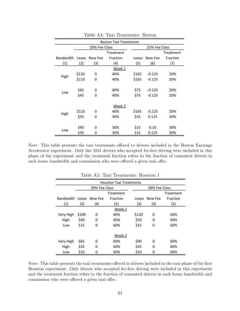
Table A4: Taxi Treatments: Boston

Bandwidth Lease NewFeeTreatmentFraction Lease NewFee

TreatmentFraction

(1) (2) (3) (4) (5) (6) (7)

$110 0 40% $165 -0.125 20%$110 0 40% $165 -0.125 20%

$45 0 40% $75 -0.125 20%$45 0 40% $75 -0.125 20%

$110 0 40% $165 -0.125 20%$55 0 30% $35 0.125 30%

$40 0 30% $15 0.10 30%$35 0 30% $15 0.125 30%

BostonTaxiTreatments

High

Low

High

Low

25%FeeClass

Week1

Week2

20%FeeClass

Note: This table presents the taxi treatments offered to drivers included in the Boston EarningsAccelerator experiment. Only the 1031 drivers who accepted fee-free driving were included in thisphase of the experiment and the treatment fraction refers to the fraction of consented drivers ineach hours bandwidth and commission who were offered a given taxi offer.

Table A5: Taxi Treatments: Houston 1

Bandwidth Lease NewFeeTreatmentFraction Lease NewFee

TreatmentFraction

(1) (3) (4) (5) (3) (4) (5)

VeryHigh $100 0 60% $120 0 60%High $40 0 60% $50 0 60%Low $15 0 60% $15 0 60%

VeryHigh $65 0 60% $90 0 60%High $35 0 60% $35 0 60%Low $10 0 60% $10 0 60%

28%FeeClass

Week2

HoustonTaxiTreatments

Week1

20%FeeClass

Note: This table presents the taxi treatments offered to drivers included in the taxi phase of the firstHouston experiment. Only drivers who accepted fee-free driving were included in this experimentand the treatment fraction refers to the fraction of consented drivers in each hours bandwidth andcommission who were offered a given taxi offer.

61

Table A6: Opt-In Rates

All Low High VeryHigh Experienced Inexperienced35or

YoungerOlderthan

35(1) (2) (3) (4) (5) (6) (7) (8)

Opt-In 0.61*** 0.58*** 0.63*** 0.65*** 0.61*** 0.61*** 0.59*** 0.63***(0.02) (0.03) (0.02) (0.03) (0.02) (0.02) (0.03) (0.02)

Observations 3130 1004 2126 1076 1732 1398 998 2144

Opt-In 0.73*** 0.67*** 0.75*** 0.78*** 0.80*** 0.69*** 0.64*** 0.76***(0.01) (0.03) (0.02) (0.02) (0.02) (0.02) (0.03) (0.02)

Observations 2096 698 1398 698 692 1404 556 1540

ByHoursGroup ByBaselineTrips ByAge

A.MaleDrivers

B.FemaleDrivers

Note: This table presents opt-in rates for fee-free driving in the first Houston experiment. The opt-in rates are adjusted for the strataused for random assignment. Levels of significance: *10%, ** 5%, and *** 1%.

62

Table A7: Frisch Elasticities Without Covariates

Low High VeryHigh Experienced Inexperienced 35orYounger

Olderthan

35 40+Hours

Weekday

Afternoon

NoLate

Nights

(1) (2) (3) (4) (5) (6) (7) (8) (9) (10)

LogWages*Male 0.40 0.46** 0.40 0.29 0.38 0.40* 0.73** 0.33 0.35* 0.35

(0.31) (0.20) (0.25) (0.19) (0.28) (0.21) (0.31) (0.25) (0.20) (0.33)

LogWages*Female 1.13*** 0.75*** 1.06*** 1.12*** 0.56** 0.96*** 0.75*** 0.78*** 0.71*** 0.73***

(0.26) (0.15) (0.27) (0.20) (0.25) (0.15) (0.17) (0.25) (0.15) (0.22)

p-valueforequality 0.059 0.225 0.063 0.001 0.617 0.024 0.944 0.182 0.140 0.302

Drivers 406 1151 604 1018 414 1140 539 414 843 478

Observations 1115 3535 1938 3062 1182 3458 1588 1337 2766 1303

DOFILE:frisch.do

UsualHoursByHoursGroup ByMonthsonPlatform ByAge

Note: All models control for the strata used for random assignment and for date fixed effects, both of which are interacted with gender.The p-values for the 2SLS and LIML models come from stacked models where the coefficient on each covariate is allowed to vary by sex.Table 5 presents analogous results, controlling for baseline covariates. Standard errors are clustered by driver. Levels of significance:*10%, ** 5%, and *** 1%.

63

Table A8: Probit Coefficients

Probit IV-Probit Probit IV-Probit(1) (2) (3) (4)

Log(Bonus)MaleNon-Shifters 0.633*** 0.779*** 0.614*** 0.787***

(0.063) (0.108) (0.062) (0.103)MaleShifters 0.672*** 0.703*** 0.634*** 0.621***

(0.007) (0.014) (0.008) (0.015)FemaleNon-Shifters 0.550*** 0.650*** 0.504*** 0.612***

(0.132) (0.199) (0.131) (0.191)FemaleShifters 0.679*** 0.713*** 0.644*** 0.660***

(0.015) (0.028) (0.015) (0.027)

Log(Threshold)MaleNon-Shifters -1.352*** -1.500*** -1.301*** -1.451***

(0.091) (0.122) (0.088) (0.118)MaleShifters -1.167*** -1.218*** -1.093*** -1.078***

(0.034) (0.039) (0.034) (0.041)FemaleNon-Shifters -1.327*** -1.442*** -1.254*** -1.355***

(0.181) (0.218) (0.177) (0.218)FemaleShifters -1.263*** -1.316*** -1.187*** -1.198***

(0.039) (0.047) (0.038) (0.048)

Observations 1047998 1047998 1047998 1047998

ProbitCoefficientsUnweighted Weighted

Note: This table presents probit coefficients from equation 13. The corresponding elasticities arepresented in Table 10. Standard errors are clustered by driver. Levels of significance: *10%, **5%, and *** 1%.

64

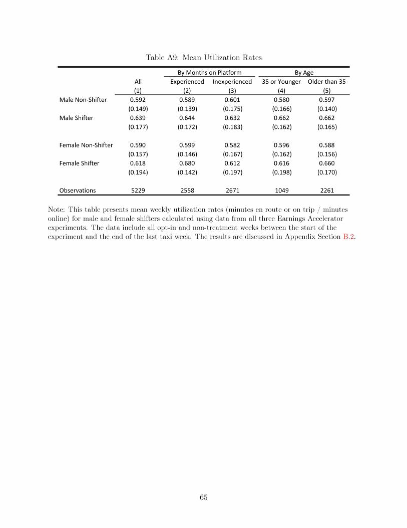
Table A9: Mean Utilization Rates

All Experienced Inexperienced 35orYounger Olderthan35(1) (2) (3) (4) (5)

MaleNon-Shifter 0.592 0.589 0.601 0.580 0.597(0.149) (0.139) (0.175) (0.166) (0.140)

MaleShifter 0.639 0.644 0.632 0.662 0.662(0.177) (0.172) (0.183) (0.162) (0.165)

FemaleNon-Shifter 0.590 0.599 0.582 0.596 0.588(0.157) (0.146) (0.167) (0.162) (0.156)

FemaleShifter 0.618 0.680 0.612 0.616 0.660(0.194) (0.142) (0.197) (0.198) (0.170)

Observations 5229 2558 2671 1049 2261

ByMonthsonPlatform ByAge

Note: This table presents mean weekly utilization rates (minutes en route or on trip / minutesonline) for male and female shifters calculated using data from all three Earnings Acceleratorexperiments. The data include all opt-in and non-treatment weeks between the start of theexperiment and the end of the last taxi week. The results are discussed in Appendix Section B.2.

65

Table A10: Mean Utilization Rates by City

All Experienced Inexperienced 35orYounger Olderthan35(1) (2) (3) (4) (5)

MaleNon-Shifter 0.639 0.628 0.649 0.633 0.640(0.194) (0.191) (0.199) (0.197) (0.194)

MaleShifter 0.662 0.680 0.641 0.662 0.662(0.164) (0.145) (0.181) (0.162) (0.165)

FemaleNon-Shifter 0.610 0.610 0.611 0.654 0.599(0.210) (0.256) (0.194) (0.152) (0.225)

FemaleShifter 0.643 0.681 0.623 0.616 0.660(0.183) (0.147) (0.197) (0.198) (0.170)

Observations 1495 744 751 537 947

MaleNon-Shifter 0.583 0.584 0.577 0.569 0.590(0.137) (0.132) (0.158) (0.158) (0.126)

MaleShifter 0.617 0.611 0.624(0.186) (0.187) (0.184)

FemaleNon-Shifter 0.590 0.599 0.581 0.595 0.588(0.156) (0.144) (0.166) (0.162) (0.154)

FemaleShifter 0.611 0.675 0.610(0.196) (0.100) (0.197)

Observations 3734 1814 1920 512 1314

ByMonthsonPlatform ByAge

B.Houston

A.Boston

Note: This table presents mean weekly utilization rates (minutes worked / minutes active) formale and female shifters calculated using data from all three Earnings Accelerator experiments.The data include all opt-in and non-treatment weeks between the start of the experiment and theend of the last taxi week. The results are discussed in Appendix Section B.2. Levels ofsignificance: *10%, ** 5%, and *** 1%.

66

Table A11: Treatment Effects on Utilization

All Experienced Inexperienced35or

Younger Olderthan35(1) (2) (3) (4) (5)

Non-Shifters -0.01** -0.01 -0.01** -0.01 -0.02**(0.01) (0.01) (0.01) (0.01) (0.01)

Shifters -0.02*** -0.03*** -0.02*** -0.01 -0.02***(0.01) (0.01) (0.01) (0.01) (0.01)

Observations 12686 4384 8302 3155 6699

EffectonUtilizationforShiftersandNon-ShiftersByMonthsonPlatform ByAge

Note: This table presents estimates of the impact of treatment offers on utilization rates. Theresults are discussed in Appendix Section B.2. Levels of significance: *10%, ** 5%, and *** 1%.

67

Table A12: IDB: Treatment Effects

All Male Female All Male Female All Male Female

(1) (2) (3) (4) (5) (6) (7) (8) (9)

LowBonusMean 29.587 30.654 23.166 0.378 0.387 0.323 49.496 51.553 37.156

Non-Shifter 1.199*** 1.486*** 1.118 0.050*** 0.050*** 0.06** 11.990*** 12.269*** 11.437***

(0.403) (0.391) (0.789) (0.011) (0.011) (0.028) (1.413) (1.554) (3.050)

Shifter 1.524*** 1.636*** 1.282*** 0.054*** 0.055*** 0.051*** 14.552*** 15.018*** 11.924***

(0.048) (0.045) (0.100) (0.001) (0.001) (0.003) (0.158) (0.170) (0.383)

Observations 845080 731483 113597 845080 731483 113597 845080 731483 113597

AboveThresholdTrips IDBPayout

Note: The first row shows the mean outcome among all observations where the driver was offered the “low” bonus. Subsequent rowsshow the impact of the high bonus treatment on outcomes for non-shifters and shifters. All models control for date fixed effects, thestrata used in Table 4, and one lag of trips. Standard errors are clustered by driver. The results are discussed in Appendix Section B.3.68

B Supplementary Results

B.1 Robustness of Intensive Margin Elasticities

We consider two alternative explanations for our finding that women are more elastic than

men on the intensive and extensive margins: differences in family responsibilities and differ-

ences in the availability of alternative jobs. We do not find any evidence for either of these

explanations.

One concern is that changes in hours worked on Uber represent shifts in hours from

alternative jobs. While we are able to rule out shifting from Lyft, Uber’s main competitor

in the marketplace, it is possible that Uber drivers have other sources of employment. In

order to bias our estimates, however, the hours at these alternative jobs would need to be

changeable at relatively high frequency (within a week) and differ by gender. We are not

aware of any evidence that female Uber drivers are more engaged in other types of flexible

work than their male counterparts. However, to address this concern we re-estimate the

elasticities within a group of drivers whom we observe working more than forty hours per

week in any of the four weeks of data we used to sample drivers. It is unlikely that this group

of workers has substantial outside (non-Uber) employment. Column 7 of Table 6 shows that

the gap between male and female elasticities shrinks, but that there is still a large difference

between the responsiveness of male and female Uber drivers in this group.

Another possibility is that even conditional on the number of hours worked, women may

be less able to adjust their hours due to family responsibilities. These constraints on women’s

hours would lead us to under-estimate their labor supply elasticities, and under-state the

differences between their behavior and that of men. To address this concern, we identify

a sample of women who typically drive during hours when we think family responsibilities

may loom large: women who regularly work between 3 and 7 P.M. on week-days. We then

re-estimate equation 6 within this subsample. Column 8 of Table 6 shows that the gap in

male-female elasticities is qualitatively similar in this subsample.

69

B.2 Utilization

We can look for suggestive evidence of platform shifting by comparing the utilization rates of

shifters and non-shifters. While switching between the Lyft and Uber apps at low frequency

will not impact utilization rates, multi-apping (running both apps at the same time) will

allow drivers to achieve a higher Uber utilization rate (and as a result higher hourly earnings

when considering earnings from multiple platforms) by spending less time idle between trips.

Table A9 presents suggestive evidence of higher utilization rates among shifters, consistent

with multi-apping. The gap is slightly larger for men than for women. The fact that young

drivers (those under 35) seem to have larger gaps in utilization is consistent with young

people being more adept with technology.

This pattern is not driven by city differences in utilization rates. Table A10 breaks down

the results for Boston and Houston. While the Houston shifters and non-shifters necessarily

come from different weeks, which could have different utilization rates due to customer

demand, the Boston results show that there are still gaps between shifters and non-shifters

when we compare utilization rates within a single city and week.

We can look for more evidence of multi-apping by comparing the impact of the treatment

on utilization rates of shifters and non-shifters. Assuming drivers first pick the “best” hours in

a day to drive, and slowly move down the utilization curve (perhaps conditional on personal

hours constraints), treated compliers should see a decrease in utilization rates, relative to

untreated compliers. Because shifters move a greater number of hours to the Uber platform

they should see a larger decrease in utilization rates.

Table A11 shows that this is indeed the case. Specifically, it presents estimates of β from:

utilizationit = βOffer + γt +Xit + εit

where Offer is the experimental percentage increase in wages. The sample is a pooled sample

that includes drivers in all three Earnings Accelerator experiments. Column 1 shows that

both shifters and non-shifters have lower utilization rates when they are treated. This is

consistent with the fact that, as drivers work more hours, they start to work less valuable

hours (with lower utilization rates). The fact that the impact is larger for shifters is consistent

with these drivers having artificially high utilization rates pre-treatment, due to multi-apping.

70

When they receive the Earnings Accelerator wage increase, they decide to shift all (or most)

of their hours to Uber, even though this means lower utilization rates on both marginal and

infra-marginal hours. We see a similar pattern across subgroups of drivers defined by driver

experience or age. It is somewhat hard to interpret the magnitudes, because, depending on

the usual number of hours worked shifters and non-shifters (or men and women) may be on

parts of the utilization curve with very different slopes.

B.3 IDB Treatment Effects

Table A12 presents treatment effects for four groups of drivers, defined by sex and whether

the driver is eligible to drive for Lyft (based on the age of their car). Specifically, we estimate

yit = βSTreatedit × Shifti + βNTreatedit × Non− Shifti +Xit + εit (15)

where Treatedit is an indicator for whether individual i is in the high bonus group in period

t, Shifti is an indicator for whether the driver has a car that allows them to drive for Lyft,

γt is a full set of date fixed effects, and Xit includes one lag of trips, and the strata used for

random assignment. Standard errors are clustered by driver. Because high and low offers are,

conditional on strata, as good as randomly assigned, this specification allows us to measure

the impact of a high offer on drivers’ labor supply, relative to the impact of a low offer.

The first three columns present estimates of βN and βS when we use total trips completed

as the outcome variable. Column 1 shows that shifters who receive the high bonus complete

1.5 additional trips; non-shifters who receive the high bonus complete 1.2 additional trips.

Columns 2 and 3 show that among both male and female drivers, shifters increase their

labor supply more than non-shifters in response to the high offer. While the difference

between shifters and non-shifters is not statistically significant, this is not surprising, given

the structure of the promotion. The promotion only incentivizes drivers to complete more

trips if they believe they are able to cross the threshold. Furthermore, there is no incentive

to drive more once the driver has crossed the threshold.

Columns 4-6 present estimates of equation 15 where 1{cross threshold} is the outcome

variable. Shifters who receive the high bonus are 5.5 percentage points more likely to cross

the threshold, relative to 5.0 percentage points for non-shifters. However, the difference is

71

not statistically significant. This largely reflects the fact that we have not exploited week

to week and driver to driver variation in the strength of the incentive. We start to see a

significant difference between shifters and non-shifters when we look at the amount of the

bonus drivers receive.28

28The fact that male shifters and non-shifters in the high bonus group appear to benefit more (in dollarterms) than their female counterparts reflects both differences in labor supply, and the fact that the maledrivers are more concentrated in the lucrative, high-threshold groups.

72

C Empirical Appendix

C.1 Construction of Hours and Earnings

Hours A driver is considered to be working whenever their Uber app is on and they have

indicated that they are available for a dispatch. This includes three distinct periods: time

waiting for a trip, time traveling to a pickup, and time on a trip. The utilization rate is the

fraction of hours spent in the second two periods.

Earnings Uber distinguishes between gross earnings– which include promotional incen-

tives—and net earnings—which subtract the amount the driver paid in Uber fees. Both of

these measures are not net of costs the driver may incur, including gas or depreciation to

the driver’s vehicle. We focus on gross earnings.

C.2 The Earnings Accelerator

This section provides more detail on the implementation of the three Earnings Accelerator

experiments. The first experiment was conducted in fall 2016 in Boston and was analyzed

in Angrist, Caldwell and Hall (2017). The second and third experiments were conducted in

Houston and have not been used in other work.

C.2.1 Boston: Fall 2016

In August-October 2016, we conducted the first of our three Earnings Accelerator experi-

ments. As in both subsequent experiments, there were three phases: (1) the selection of

eligible drivers, (2) “fee-free” offers, and (3) taxi offers. Table 1 lists the timeline for the

three phases.

Drivers were eligible for inclusion in the Boston experiment if they had completed at least

4 trips in July 2016 (were “active” drivers) and if their average hours per week, conditional

on driving, were between 5 and 25 hours per week. We excluded very high hours drivers

to reduce the cost of the experiment. We grouped drivers into two bandwidths based on

their average hours per week. “Low-hours” drivers drove an average of 5-15 hours/week and

“high-hours” drivers drove an average of 15-25 hours/week. Roughly 45% of Boston drivers

73

were eligible for inclusion in the experiment.

We randomly selected 1600 eligible drivers for inclusion in the experiment within strata

defined by average hours driven in July, driver fee class (commission rate), and vehicle model

year. All of these drivers were offered one week of fee-free driving. Half were offered fee-free

driving one week (wave 1); half were offered it in the next week (wave 2). Column 3 of Table

A1 shows that drivers offered fee-free driving in wave 1 were statistically indistinguishable

from those offered fee-free driving in wave 2. Drivers were notified about the Earnings Ac-

celerator offer via e-mails, text message, and in-app notification. The in-app notification

stayed at the top of each driver’s Uber app for the entire opt-in period, and drivers received

reminder e-mails and text messages throughout the week. Figure A3 shows sample messag-

ing. Each message contained a link to a Google Form, which provided more information

on the incentive. In particular, this form indicated the exact time the incentive would be

active (Monday 4 A.M. for one week, following the standard Uber week) and informed the

drivers that if they opted in to the Earnings Accelerator, their data would be used by aca-

demic researchers. One thousand and thirty-one of the 1600 drivers chose to opt-in to the

promotion.

At the time we ran the experiment, drivers’ trip receipts typically showed three things:

the amount collected from the rider, the amount collected by Uber (due to the proportional

fee), and the amount they were paid (the difference between the two). Drivers who accepted

the offer of fee-free driving were able to see in-app that their fees were zero (see Figure A6

for a sample trip receipt). They also received e-mail, text message, and in-app reminders

throughout the week that the “Earnings Accelerator [was] on” and that they were earning

more on every trip. The messaging was crafted so as to mimic that used for standard Uber

promotions.

Drivers who opted in to fee-free driving were included in the third phase of the exper-

iment, the Taxi treatments. In each of two weeks, we offered drivers the opportunity to

buy additional weeks of fee-free driving for a pre-specified cost. Table A4 shows the Taxi

contracts offered in each of the two weeks, along with the probability of selection and the

percentage of drivers who accepted our offers. Columns 4 and 5 of Table A1 shows that the

taxi treatment and control groups were balanced during both weeks of treatment.

In each week we offered two types of taxi contracts, where the lease varied by hours

74

bandwidth and commission. In the first week some drivers received the opportunity to buy

an additional week of fee-free driving; others received the opportunity to buy a week of

negative fee (-.125%) driving. Offers in the second week were less generous, but were priced

accordingly. The e-mails and opt-in forms contained information on the “break-even” a driver

must exceed (in terms of gross earnings) to make buying the contract worthwhile. They also

contained links to online calculators that allowed the drivers to calculate their earnings with

and without the Earnings Accelerator. A screenshot from one of these calculators is shown in

Figure A7. Driver who accepted the offer had the lease payment subtracted from their opt-in

week earnings statement, as shown in Figure A8. They saw their increased earnings in-app,

just as they did during fee-free week, with one exception: drivers who bought a “negative fee”

contract during the first Boston Taxi week. It was not possible to implement a negative fee

using the Uber platform. These drivers saw no fee in-app and received additional text and

email reminders that they would receive an additional 12.5% on their weekly pay statement.

C.2.2 Houston: Spring 2017

In spring 2017 we conducted a second round of the Earnings Accelerator in Houston, Texas.

Uber launched operations in Houston in July 2013 and by the spring of 2017 had over 15,000

active drivers (drivers who had completed at least four trips in the previous month). Lyft

entered the market in February 2014 but suspended operations in August 2017 after the

Houston City Council passed new TNC regulations which mandated a stricter background

check for drivers. They had fully withdrawn from the Houston market by November 2017.

Uber remained operational in Houston despite the new regulation.

Relative to the Boston experiment, there were two key modifications. First, we included

a third hours group, including drivers who drove between 25 and 40 hours per week on

average in the month prior to the experiment. These drivers had been omitted from the

Boston experiment due to budgetary considerations. Their inclusion allowed us to examine

the responsiveness of drivers who were working more than part-time on the Uber platform.

Second, we over-sampled female drivers so that we could explore gender differences in labor

supply elasticities.

Drivers were eligible for inclusion in the first Houston experiment if they completed at

least 4 trips in the prior month (were “active” drivers) and if their average hours per week,

75

conditional on driving, were between 5 and 40 hours per week in the month before the

experiment. Within this sample of eligible drivers, we randomly selected 2020 drivers for

inclusion in the experiment within six strata defined by the interaction of hours bandwidth

and gender. The messaging and notifications mirrored that of the Boston experiment. As

before, we offered half of the drivers the opportunity to drive fee-free in one week, and the

other half of the drivers the same opportunity the next week. Column 3 of Table A2 shows

that drivers offered fee-free driving in wave 1 were statistically indistinguishable from those

offered fee-free driving in wave 2. One thousand, three hundred and fifty-five drivers accepted

our offer and were included in the third phase of the experiment.

Table A5 shows the taxi contracts offered in each of the two Taxi weeks, along with the

probability of selection and the percentage of drivers who accepted our offers. Due to the

addition of the third hours bandwidth and logistical constraints on the number of treatments

we could implement at a single time, we eliminated the negative and half fee treatments and

only offered drivers the opportunity to buy weeks of fee-free driving. Columns 4 and 5 of

Table A2 shows that the taxi treatment and control groups were balanced during both weeks

of treatment.

C.2.3 Houston: Fall 2017

We conducted a third round of the Earnings Accelerator several months after Lyft re-entered

the Houston market. In May 17, 2017, the Texas State Legislature passed bill, H.B. 100, with

a super-majority in the Senate (21-9), and on May 29, the Governor signed it, immediately

removing mandatory fingerprinting. Lyft announced its intention to resume operations and

re-entered Houston at 2 p.m. C.T. on May 31, 2017.

The second Houston experiment was hampered by a number of implementation issues,

which complicate the analysis. First, the experiment took place only a few weeks following

Hurricane Harvey, which flooded much of Houston. While we made every attempt to recruit

drivers who were not affected by the hurricane, we saw significantly lower opt-in rates than

we saw in either Boston or in our first Houston experiment, suggesting that some drivers may

not have fully recovered. Second, changes to the Uber app made it impossible to implement

the increased wages in the usual manner, except during the first week of fee-free driving.

Drivers were eligible for inclusion in the third iteration of the Earnings Accelerator if –

76

as before – they had completed at least four trips in the prior month (were “active” drivers),

if their average hours per week, conditional on driving, were between 5 and 40 hours per

week, and if they had completed a trip in Houston after Uber re-started operations following

Hurricane Harvey.29 The messaging, notifications, and timeline were similar to the first

Houston experiment. The one key change was reference to Uber’s fee: Uber changed its

policy in June 2017 to loosen the link between rider fares and driver earnings—this was

called “up front pricing”—and removed the concept of the Uber “fee”. What drivers earned

per trips did not change; it remained a function of a base fare plus a per-mile rate and a

per-minute rate. As a result, we did not mention the “Uber fee” in the second Houston

experiment. Instead we focused our messaging on the proportional increase in earnings.

Column 3 of Table A3 shows that drivers were balanced across waves one and two.

We included 2100 drivers in the second Houston experiment. In the first treatment,

drivers received one of four multipliers on total earnings at no cost (the equivalent of fee-free

driving): 1.2x, 1.3x, 1.4x, and 1.5x. The first wave were offered the multiplier in the week

of September 18 and saw the treatment in-app (as a proportional increase in the base fare,

per-mile rate, and per-minute rate). Due to technical constraints, the second wave—who

were offered the multiplier in the week of September 25—did not see the treatment in-app

and instead received a lump-sum bonus at the end of the week. A total of 1270 drivers

accepted our “fee-free” offer and were included in the third (“taxi”) phase of the experiment,

a single week of Taxi offers. We do not include data from the second phase in our analysis

as it is not comparable to earlier experiments due to significant changes in the driver app.

C.3 Individual Driver Bonuses

The complexity of the algorithm Uber uses to assign in the IDB program generates random

variation in assignment to high and low bonus offers, conditional on prior driving behavior.

We group drivers into eight hours bins based on their driving behavior in the prior four

weeks. In Table 4 We show that conditional on these eight strata, there is no statistical

difference between drivers in the high and low offer groups.

29The total volume of trips had rebounded to pre-hurricane levels by the time we conducted the experiment,but we did not want to include drivers who had stopped driving because they had been personally impactedby the hurricane.

77

D Theoretical Appendix

D.1 Firm- and Market- Labor Supply Elasticities

Consider a simple intertemporal labor supply model where individuals can work for two jobs.

Hours at the first job are denoted ht and hours at the second job are denoted rt. At time t,

individuals choose consumption, ct, and hours {ht, rt} to maximize the present discounted

value of future utility. Their instantaneous utility function, u(ct, lt) depends on consumption

and leisure where lt = T −ht− rt. Utility is increasing in both consumption and leisure and,

as is standard, as ct → 0, uc →∞.

Individuals earn an exogenous income stream yt and face a constant (within period) wage

rate wt at their main job. At their second job, rt hours nets them L(rt) in earnings where

L(·) is concave. Individuals can borrow and save, and face no borrowing constraints. Assets

in period t are denoted At. As in standard labor supply models, since utility is additive we

can write the problem recursively as

Vt(At) = maxct,ht,rt

u(ct, T − ht − rt) + βEt[Vt+1(At+1)]

subject to

ht, rt ≥ 0

At+1 = (1 +Rt)(At + yt + wtht + L(rt)− ct − κ1{rt > 0})

AT = 0

where κ is the psychic cost of working multiple jobs.

The model yields simple predictions for the responsiveness of hours at both the main and

second job to changes in the main job’s wage and in the cost of working on two jobs. The

intra-temporal conditions are:

wt =ul + µh

t

uc

L′(rt) =ul + µr

t

uc

78

where the µt are the Lagrange multipliers on the constraint that hours in both jobs must be

greater than or equal to zero. Assuming an interior solution for hours at the main job, hours

are chosen to equate the ratio of the marginal utilities of leisure and consumption (taking

into account jobs at the second job) to the wage. This simple set-up yields three intuitive

predictions.

Proposition 3. Conditional on working a second job, hours in the second job are decreasing

in wt.

Proof. We can rearrange the first order conditions to see that L′(rt)−wt = 0. By the implicit

function theorem∂rt∂wt

=1

L′′(rt)

and since L is concave, rt is decreasing in wt.

Proposition 4. If the second job’s hours are not flexible, the response of total hours worked

is the same as the response of hours worked at the main job.

Proof. If the second job’s hours are fixed, dr/dw = 0.

This proposition allows us to ignore non-gig employment when estimating labor supply

elasticities in markets where Lyft is unavailable. While the Uber drivers in our data may

work traditional jobs (just like taxi drivers or stadium vendors), as long as they are not

able to change their hours at these jobs at high frequency (within a week), our estimates of

market labor supply elasticities will reflect real increases in hours worked.

Proposition 5. The elasticity of hours worked at the main job with respect to the wage is

greater than the elasticity of total hours worked.

Proof. This follows from propositions 3 and 4. Temporarily drop the time subscripts and

define H = h + r and φ =h

H(fraction of total hours spent at the primary job). We can

write

dH

dw

w

H=

dh

dw

w

H+dr

dw

w

H

=dh

dw

w

φH(1/φ)+dr

dw

w

H(1− φ)/(1− φ)

ε = τφ︸︷︷︸+

+(1− φ) s︸︷︷︸−

79

The first term is positive. The second term is negative by Proposition 3

Propositions 3 and 5 show that if individuals can shift hours between employers easily,

estimates of the labor supply elasticity using a single platform will conflate changes in hours

supplied to the market and changes in the allocation of hours across firms .

D.2 Derivation of the First Stage

This section goes through a derivation of the first stage. A similar derivation is provided in

the main text of Angrist, Caldwell and Hall (2017).

The first stage effect of offers on log wages depends on: (1) the experimental participation

rate, and (2) the magnitude of experimentally-induced fee changes. Use w0it to denote a

driver’s potential average hourly earnings in the absence of treatment and t0 to denote the

driver’s Uber fee. Then, using the potential outcomes framework, the hourly earnings we

observe satisfy:

wit = w0it(1− t0)(1−Dit) + w0

it(1− t1)Dit

= w0it(1− t0) + w0

it(t0 − t1)Dit.

where Dit is a binary indicator for whether the driver is driving fee-free. Because offers, Zit

are independent of w0it , the first stage effect of offers on wages is

E[wit|Zit = 1, t0, t1]− E[wit|Zit = 0, t0, t1]

= (t0 − t1)E[w0it|Dit = 1]× P [Dit = 1|Zit = 1]. (16)

The first stage impact on wages is just the experimental fee change multiplied by the opt-in

rate and wages for non-participants.30

The proportional change in wages is obtained by dividing (16) by the wages of the controls,30The derivation here uses the fact that Dit = 1 implies Zit = 1, which in turn yields E[w0

it|Dit = 1, Zit =1] = E[w0

it|Dit = 1].

80

E[wit|Zit = 0] = E[w0it](1− t0). The proportional wage increase is:

E[wit|Zit = 1, t0, t1]− E[wit|Zit = 0, t0, t1]

E[wit|Zit = 0, t0, t1]

=(t0 − t1)1− t0

P [Dit = 1|Zit = 1]. (17)

In other words, the first stage for log wages is the change in fee divided by the baseline

take-home rate (1-fee), multiplied by the treatment take-up rate. For example, with a take-

up rate of 2/3, the proportional first stage for an experiment that eliminates a 25% fee is

roughly .25.75.66 = .22.31

D.3 Individual Driver Bonuses and Labor Supply Elasticities

Use ti0 to denote the number of trips driver i completes when untreated (given the “low”) offer

and ti1 to denote the number of trips driver i completes when treated. Given the structure

of the treatment, there are three possible cases:

1. If ti0 ≥ T , the driver already exceeds the trip threshold. Assuming no income effects,

his/her labor supply is unaffected and ti1 = ti0.

2. If ti0 < T and ti0(1 + εB/T

w) < T , ti1 = ti0 where ε =

d log t

d logwis the elasticity of trips

with respect to the per trip wage. Assuming a reasonably constant number of trips

per hour, ε is also equivalent to the elasticity of hours worked to the wage. The driver

is either too far below the trip threshold or not elastic enough to reach the threshold.

His labor supply is unaffected.

3. If ti0 < T and ti0(1 + εB/T

w) ≥ T , ti1 = T . The driver is close enough to the trip

threshold and elastic enough to reach the trip threshold.

This can be summarized by the following:

ti1 =

ti0 if ti0 ≥ T

ti0 if ti0(1 + εB/T

w) < T

T otherwise

31The first stage in logs is ln 1−t11−t0

× P [Dit = 1|Zit = 1], but ln 1−t11−t0

≈ (t0−t1)1−t0

.

81

and

ti1 ≥ T ⇐⇒ ti0(1 + εB/T

w) ≥ T

If pB,T is the opt-in rate among the high-bonus group we can rewrite this as

pB,T = 1− F0 [T/(1 + ε(B/T )/w)]

1− pB,T = F0 [T/(1 + ε(B/T )/w)]

F−10 [1− pB,T ] = T/(1 + ε(B/T )/w)

D.3.1 Estimation Procedure

We estimate ε using the following procedure: we group drivers into strata based on: sex,

shifter/non-shifter, and date.

1. We calculate the number of drivers in the high bonus group that exceeded the trip

threshold. We denote this pB,T

2. We find the 1− pB,T quantile of the corresponding low bonus group

3. We fit equation 14 by non-linear least squares. We allow the elasticity to vary across

the four groups.

4. We bootstrap steps 1-3 500 times to obtain standard errors.

82