East Tennessee State UniversityDigital Commons @ East

Tennessee State University

Electronic Theses and Dissertations Student Works

12-2005

Monitoring PC Hardware Sounds in LinuxSystems Using the Daubechies D4 Wavelet.Robert Karns HenryEast Tennessee State University

Follow this and additional works at: https://dc.etsu.edu/etd

Part of the Computer Sciences Commons

This Thesis - Open Access is brought to you for free and open access by the Student Works at Digital Commons @ East Tennessee State University. Ithas been accepted for inclusion in Electronic Theses and Dissertations by an authorized administrator of Digital Commons @ East Tennessee StateUniversity. For more information, please contact digilib@etsu.edu.

Recommended CitationHenry, Robert Karns, "Monitoring PC Hardware Sounds in Linux Systems Using the Daubechies D4 Wavelet." (2005). ElectronicTheses and Dissertations. Paper 1076. https://dc.etsu.edu/etd/1076

Monitoring PC Hardware Sounds in Linux Systems Using the Daubechies D4 Wavelet

A thesis

presented to

the faculty of the Department of Computer Science

East Tennessee State University

In partial fulfillment

of the requirements for the degree

Master in Applied Computer Science

by

Robert K. Henry

December, 2005

David Tarnoff, Chair

Phillip Pfeiffer

Jeff Knisley

Keywords: Wavelet, Daubechies, DSP, Monitor, S.M.A.R.T., ALSA, Linux, failure prediction, remote, vibration analysis

ABSTRACT

Monitoring PC Hardware Sounds in Linux Systems Using the Daubechies D4 Wavelet

by

Robert K. Henry

Users of high availability (HA) computing require systems that run continuously, with little or no

downtime. Modern PCs address HA needs by monitoring operating system parameters such as

voltage, temperature, and hard drive status in order to anticipate possible system failure.

However, one modality for PC monitoring that has been underutilized is sound. The application

described here uses wavelet theory to analyze sounds produced by PC hard drives during

standard operation. When twenty-nine hard drives were tested with the application and the

results compared with the drives’ Self-Monitoring, Analysis, and Reporting Technology

(S.M.A.R.T.) data, the binomial distribution’s low p-value of 0.012 indicated better than chance

agreement. While the concurrence between the two systems shows that sound is an effective tool

in detecting hardware failures, the disagreements between the systems show that the application

can complement S.M.A.R.T. in an HA system.

2

COPYRIGHT

Copyright 2005 by Robert K. Henry

All Rights Reserved

3

ACKNOWLEDGEMENTS

Thank you to the members of the thesis committee for your time and guidance in this

research.

Thank you to Dr. Terry Countermine, David Robinson, and the East Tennessee State

University seniors who worked so diligently in the ETSU “Providing Area Schools with

Technical Assistance” (PASTA) program for providing hard drives for testing. Your time and

conscientious effort in collecting the hardware components helped make this research possible.

Thank you, Dr. Edith Seier, Department of Mathematics, ETSU, for your statistical

consultation. Your advice has been helpful in designing the project and in evaluating the system.

Thank you, Professor Penny Smith, Department of Math, Lehigh University, for your

friendship, mathematical advice on wavelets, and your encouragement, without which this

project would never have begun.

Thank you to Terri Henry Briggs, my sister. Your donation of the computer for

developing the Linux software was helpful in advancing the project.

Thank you to Jo Watson Henry, my mother, for your help in proofreading.

Thank you to the ALSA Development Team for help on ALSA through articles on the

ALSA website and the ALSA mail list.

4

CONTENTS

Page

ABSTRACT..................................................................................................................................... 2

COPYRIGHT................................................................................................................................... 3

ACKNOWLEDGEMENTS............................................................................................................. 4

CONTENTS..................................................................................................................................... 5

LIST OF TABLES........................................................................................................................... 9

LIST OF FIGURES ....................................................................................................................... 10

Chapter Page

1. INTRODUCTION ..................................................................................................................... 11

1.1 Motivation for Research ...................................................................................................... 11

1.2 Results.................................................................................................................................. 12

1.3 Overview of Thesis.............................................................................................................. 14

2. BACKGROUND ....................................................................................................................... 15

2.1 Hardware Sensors ................................................................................................................ 15

2.1.1 Basic Sensors ................................................................................................................ 15

2.1.2 Self-Monitoring, Analysis, and Reporting Technology (S.M.A.R.T.) ......................... 16

2.2 Sensing Sound...................................................................................................................... 19

2.2.1 Accelerometers and Microphones................................................................................. 19

2.2.2 Sampling Sounds .......................................................................................................... 20

2.2.3 Sampling Programming Practice .................................................................................. 21

2.3 Analyzing Sounds ................................................................................................................ 23

2.3.1 Fourier Transform......................................................................................................... 23

2.3.2 Fast Fourier Transform ................................................................................................. 24

2.3.3 Localizing in Time........................................................................................................ 26

2.3.4 Wavelets........................................................................................................................ 27

5

Chapter Page

2.3.5 Haar Wavelet ................................................................................................................ 28

2.3.6 Daubechies Wavelet...................................................................................................... 30

2.3.7 Multiresolution Analysis and the Fast Wavelet Transform (FWT) .............................. 33

2.3.8 Lifting ........................................................................................................................... 37

2.3.9 Wavelet Packets ............................................................................................................ 38

2.4 Classifying Signals .............................................................................................................. 39

2.5 Wavelet Software Solutions................................................................................................. 39

2.6 Summary.............................................................................................................................. 42

3. METHODOLOGY .................................................................................................................... 43

3.1 Software Specification......................................................................................................... 43

3.2 Programming Environment.................................................................................................. 43

3.3 Prototype Development ....................................................................................................... 43

3.4 Filtering................................................................................................................................ 44

3.4.1 Collection of Failed Components ................................................................................. 44

3.4.2 Obtaining Hard Drive Data ........................................................................................... 45

3.4.3 Testing of Wavelet Transform Class ............................................................................ 46

3.5 Sound Sampling................................................................................................................... 46

3.6 Classifier .............................................................................................................................. 47

3.7 Limitations ........................................................................................................................... 47

3.8 Licensing.............................................................................................................................. 48

3.9 Summary.............................................................................................................................. 48

4. THE APPLICATION................................................................................................................. 49

4.1 Overview of SonMon........................................................................................................... 49

4.2 D4 Wavelet Class................................................................................................................. 49

4.2.1 Description of Code ...................................................................................................... 50

4.2.2 Spike Signal Demonstration ......................................................................................... 52

6

Chapter Page

4.3 Main Function...................................................................................................................... 53

4.4 Callback Function ................................................................................................................ 53

4.5 Classify Function ................................................................................................................. 54

4.5.1 Histogram...................................................................................................................... 54

4.5.2 Chi-Square Comparison................................................................................................ 55

4.6 Templates............................................................................................................................. 55

4.7 Summary.............................................................................................................................. 56

5. RESULTS .................................................................................................................................. 57

5.1 Introduction.......................................................................................................................... 57

5.2 S.M.A.R.T. Test Procedure.................................................................................................. 58

5.3 S.M.A.R.T. Test Evaluation ................................................................................................ 59

5.4 SonMon Test Results ........................................................................................................... 59

5.5 Evaluation of Results ........................................................................................................... 62

5.5.1 Agreement of Observers Test, Kappa........................................................................... 63

5.5.2 Probabilities of Disagreement....................................................................................... 64

5.5.3 Binomial Distribution ................................................................................................... 64

5.6 Improving Performance ....................................................................................................... 64

5.6.1 Templates ...................................................................................................................... 64

5.6.2 Threshold Value............................................................................................................ 65

5.6.3 Histograms .................................................................................................................... 68

5.7 Summary.............................................................................................................................. 69

6. CONCLUSIONS........................................................................................................................ 70

Future Work............................................................................................................................... 70

REFERENCES .............................................................................................................................. 72

APPENDICES ............................................................................................................................... 74

Appendix A: Glossary ............................................................................................................... 74

7

Chapter Page

Appendix B: Source Code ......................................................................................................... 75

D4.h........................................................................................................................................ 75

D4.cpp.................................................................................................................................... 77

sonmon.c ................................................................................................................................ 82

Makefile ................................................................................................................................. 90

d4dll.cpp................................................................................................................................. 91

Appendix C: Gnu General Public License................................................................................. 93

Appendix D: Results Summary ................................................................................................. 98

VITA............................................................................................................................................ 100

8

LIST OF TABLES

Table Page

1. S.M.A.R.T. Test Results ........................................................................................................... 59

2. SonMon Results ........................................................................................................................ 62

3. S.M.A.R.T. vs. SonMon ........................................................................................................... 63

4. Threshold 900 Results............................................................................................................... 66

5. S.M.A.R.T. vs. SonMon with Threshold 1100 Results ........................................................... 66

6. Threshold Values and Binomial p-values ................................................................................. 67

9

LIST OF FIGURES

Figure .........................................................................................................................................Page

1. Sample Output from smartctl.exe ...........................................................................................18

2. Input Signal.............................................................................................................................24

3. FFT Transform........................................................................................................................25

4. Transient Signal ......................................................................................................................26

5. Transient Fourier Transform...................................................................................................26

6. Haar Wavelet ..........................................................................................................................29

7. Haar Scaling Function ............................................................................................................30

8. D4 Scaling Function φ ............................................................................................................31

9. D4 Wavelet ψ..........................................................................................................................32

10. Wavelet Approximation..........................................................................................................33

11. Sine .........................................................................................................................................34

12. Haar Approximation ...............................................................................................................34

13. Multiresolution Analysis.........................................................................................................35

14. Multiresolution Tree ...............................................................................................................36

15. Wavelet Packet Tree ...............................................................................................................39

16. SonMon System Operation.....................................................................................................50

17. Wavelet Transform Of Spike ..................................................................................................53

10

CHAPTER 1

INTRODUCTION

1.1 Motivation for Research

Users of high availability (HA) computing require systems that run continuously, with

little or no downtime. One critical technology for achieving high availability is self-monitoring:

the ability of a system to detect faults and signs of abnormalities. Self-monitoring is particularly

important in environments such as massively parallel clusters, where downtime can be costly and

disruptive, and the sheer mass of hardware makes the detection of faults and failures more

complex and costly.

To make component failures easier to detect, modern computers often support data

acquisition devices (DAQ) that monitor operating characteristics such as temperature, voltage,

and fan speed. A more intelligent device, the Self-Monitoring, Analysis and Reporting

Technology (S.M.A.R.T.) System, provides data on hard drive operation; basic input/output

systems (BIOSes) and operating systems have used S.M.A.R.T. technology for years to identify

abnormalities in hard drives.

One potentially useful but underutilized modality for detecting failing components in

computers is sound. Sound has previously been used to detect abnormal system operation in

automotive and mechanical engineering. Modern automobile engine controls, for instance, use an

accelerometer to monitor vibrations caused by detonation, and then control spark advance

accordingly.1 Another project investigated using signals from accelerometers to monitor

vibration in helicopter transmissions. In this project, accelerometers installed near critical

1 Leonardo Mangeruca, Alberto Ferrari, Alberto Sangiovanni-Vincentelli, Andrea Pierantoni , Michele Pennese,

System Level Design of Embedded Controllers: Knock Detection, a Case Study in the Automotive Domain, (2003), 2, http://www-cad.eecs.berkeley.edu/Respep/Research/asves/paper2003/Mangeruca_date03.pdf (last accessed 11/8/2005)

11

bearings and gears in the transmission transmit a signal that is analyzed for potential component

failure.2

Although most computer components are not mechanical, devices such as hard drives and

cooling fans contain motors and bearings that may make abnormal sounds as they deteriorate. PC

users often request service when they hear these sounds, which in turn are often used in

troubleshooting.3, 4

In the case of cluster computing, the task of monitoring sound becomes much more

difficult. There are three reasons for this. The tendency to house these systems in dedicated

rooms precludes most users from hearing any sounds at all. Moreover, the number of PCs in

these rooms makes it less likely that people who do come near the machines will hear abnormal

noises, or if they do hear a sporadic strange noise, be able to identify the source of that noise.

1.2 Results

The research described here produced a Linux-based prototype for a sound-based system

for detecting and analyzing mechanical hard drive failures. This system uses a built-in sound

card and a microphone to obtain digital samples of hardware sounds. Once acquired and

digitized, sounds are decomposed using digital signal processing (DSP) techniques, and checked

for symptoms of potential failure.

A design consideration was that the analysis system must present a minimal processing

load on the system. This constraint was one consideration in choosing wavelet analysis as the

DSP filter. Wavelets can provide useful filtering in time O(n), where n is the sample size: a

significant performance improvement over some other DSP techniques.

2 Gary G. Yen and Kuo-Chung Lin, Wavelet Packet Feature Extraction for Vibration Monitoring, 2000, IEEE

Transactions on Industrial Electronics, Vol, 47, No. 3, 661 3 Knowledge Base Online Help Topics, “Identifying and troubleshooting hard drive noise issues”, Maxtor

Corporation, 2005, http://maxtor.custhelp.com/cgi-bin/maxtor.cfg/php/enduser/olh_adp.php?p_faqid=481 (accessed 7/26/2005)

4 Service and Support, “How can I tell if the noise or sound my drive is making is normal?”, Western Digital Corporation, 2005, http://wdc.custhelp.com/cgi-bin/wdc.cfg/php/enduser/std_adp.php?p_sid=hEQMvwLh&p_search_text=troubleshooting&p_widx=1&p_faqid=568&p_topview=1, (accessed 7/27/2005)

12

The prototype was tested on sounds from unserviceable hard drives. Digital recordings of

the hard drives were played to the application and the results from the application captured for

examination. The captured data consisted of χ2 comparisons between digitally filtered samples of

the input sound and a template prepared to represent a normal quiescent hard drive. Those χ2

results exceeding a fixed threshold were used to classify hard drives as good or bad. The

threshold was also studied to determine the optimum value for this parameter.

The results of the sound testing were compared to the S.M.A.R.T. data extracted from the

hard drives. These two sets of observations were compared using Cohen’s kappa (κ), a statistical

measure of observer agreement. Kappa corrects for agreement between the observers due to

chance but says nothing about the validity of either set of observations. Though S.M.A.R.T. is

being used to measure the validity of the sound measurement results, S.M.A.R.T. cannot be

assumed as an infallible benchmark. This makes Kappa a useful comparison tool, because it

measures the degree of agreement between two observers, either of which may be wrong.

Comparing the S.M.A.R.T. observations with the sound observations with optimized threshold

yielded a kappa as high as 0.3446, indicating a fair degree of agreement.

Agreement between the two observers was also compared using the binomial distribution.

The binomial distribution is used to calculate the probability of the observers agreeing by

chance. The p-value was computed for numbers of agreements equal or greater than observed

numbers with a binomial probability of 50%. To test for significance, the p-value should be as

low as possible. Though p-values below 0.05 are normally considered significant, the less

restrictive value of 0.10 was used for this research because of the small number of drives

available for test and because of inherent differences between sound and S.M.A.R.T. that would

make perfect agreement impossible. The binomial distribution p-value testing for agreement

between sound and S.M.A.R.T. by chance was as low as 0.012. This number indicates that there

is a 0.012 or 1.2% probability that the agreement between the observers is by chance.

These results, in short, show that sound can be used as an effective indicator for hardware

condition.

13

1.3 Overview of Thesis

The balance of this thesis is divided into five chapters. Chapter 2 discusses supporting

technologies for this work, including data acquisition, signal processing, wavelets, sampling

sound using the PC sound card under Linux, and methods of classifying wavelet data. Chapter 3

reviews the methodology and scope of the research. Chapter 4 discusses the design of the

software components used in the system prototype. Chapter 5 examines the results of

experiments with the prototype to assess the system’s effectiveness. Chapter 6 summarizes the

thesis, offering suggestions for future work.

14

CHAPTER 2

BACKGROUND

This chapter discusses the technologies on which this research is based. Topics covered

include hardware sensing technology for personal computers (PCs); the Self-Monitoring,

Analysis and Reporting Technology (S.M.A.R.T.) system for analyzing hard drive performance;

digital-signal-processing (DSP) techniques for sound analysis; and the Linux sound card

technology used in this work for handling sound samples.

2.1 Hardware Sensors

2.1.1 Basic Sensors

Large computing systems have long incorporated sensors or data acquisition (DAQ)

devices to monitor the operation of hardware. For example, in 1977, the Cray-1 computer had a

monitoring system to detect power and cooling systems malfunctions.5

In recent years, manufacturers have installed sensors in some personal computers (PCs)

to monitor physical characteristics such as temperature, voltage, and other measurable quantities

of the motherboard and peripheral devices. PC sensors obtain data on a system’s hardware and

provide that data to the host system.

An example of a common, simple sensor is National Semiconductor’s LM75 temperature

sensor.6 The LM75 incorporates a sensing element, an analog-to-digital converter (ADC), and

other digital circuitry for reporting temperatures to the processor. The sensing element delivers a

voltage signal to the ADC, which computes the digital number that represents the temperature.

The host machine reads the digital temperature measurement from the device as a 9-bit 2’s-

complement value representing temperatures from -55°C to 125°C with an accuracy of between

±2°C and ±3°C.

5 Cray-1 Hardware Reference Manual, (1977) http://www.ed-thelen.org/comp-hist/CRAY-1-HardRefMan/CRAY-

1-HRM.html#p2-8 (Accessed 10/10/2004) 6 Digital Temperature Sensor and Thermal WATCHDOG™ with Two-Wire Interface, National Semiconductor

Corporation, (1/6/2000)

15

When installed in a computer, the LM75 is mapped to an I/O port that can be queried at

any time by the host machine and the temperature read directly from the port. The LM75 can

also be configured to generate an interrupt to the host computer if the measured temperature

exceeds a specified value. In this configuration, attention from the host computer is required only

when the system's temperature is of concern. In this case, interrupt handlers on the host computer

must be designed to read the correct I/O port for the device and correctly interpret the data

obtained. This means that the software must be designed for the specific computer or must be

user configurable.

A more modern DAQ device, National Semiconductor’s multipurpose LM87 sensor, can

acquire and digitize data from several different sources. The LM87 can measure temperatures

from an on-chip sensor and accept input from two additional external temperature sensors. In

addition, the device can sample voltages, measure and control the speeds of two sensor-equipped

fans, and generate an interrupt when a parameter exceeds its tolerances.7 As in the case of the

LM75, the LM87’s software controller must be specific to the host computer’s hardware.

2.1.2 Self-Monitoring, Analysis, and Reporting Technology (S.M.A.R.T.)

An additional type of PC sensor system is the Self-Monitoring, Analysis, and Reporting

Technology (S.M.A.R.T.) found in ATA/IDE and SCSI hard drives.8 S.M.A.R.T. is based on

IBM’s technology of Predictive Failure Analysis (PFA),9 a technology that IBM first provided to

customers in 1992.10 S.M.A.R.T. sensors predict hard drive failure by measuring and analyzing a

hard drive’s operating parameters including head flying height, drive spin-up time, and

temperature. If head flying height is lower than normal, an above-average possibility of a head

crash exists. A drive that takes longer than usual to spin up may have bearings that are wearing

7 Serial Interface System Hardware Monitor with Remote Diode Temperature Sensing, National Semiconductor

Corporation, (9/11/2003), (LM87.pdf) 8 Mark Evans, SFF Committee Specification for Self-Monitoring, Analysis, and Reporting Technology, Quantum

Corporation, (4/26/1996) 9 Playing it S.M.A.R.T, Seagate.com ( ) (accessed 9/26/2004) http://www.seagate.com/support/kb/disc/smart.html10 PCTechGuide S.M.A.R.T. ( )(accessed 9/26/2004) http://www.pctechguide.com/04disks_SMART.htm

16

out.11 When the probability of failure exceeds a given threshold, the drive can warn of imminent

failure, permitting backup of data and replacement of the component before failure occurs.

Hughes, et. al. suggest that S.M.A.R.T. does not perform perfectly in reporting impending

failures without excessive false alarms due to the low failure rate for hard drives, typically

<1%/year.12

Normally, a PC’s BIOS checks S.M.A.R.T. data during the power on self-test.

Parameters that fall outside their threshold values cause the system to signal an error. In addition

to the BIOS monitoring, several software applications are available for monitoring S.M.A.R.T.

drive data. Most hard drive manufacturers provide software that reads, analyzes, or displays

S.M.A.R.T. data for their own or other manufacturers’ drives, and make these applications

available for download without cost from the manufacturer’s websites.

Vendor-supported and freeware applications are available that read, monitor, and display

hard drive S.M.A.R.T. data. An example of a free S.M.A.R.T. application is smartmontools,

released under the GNU General Public License and available for Windows as well as

UNIX/Linux.13 Figure 1 presents a smartmontools report for a drive with an excessive raw read

error rate count. This report indicates that the drive has failed and that its data should be backed

up promptly.

The information presented in S.M.A.R.T. drive reports varies, depending on the drive

manufacturer’s implementation of the S.M.A.R.T. standard. These variations may represent

choices by manufacturers to ignore parameters that have not been shown to be useful in

predicting failure for this particular device.

11 Playing it S.M.A.R.T. 12 Gordon F Hughes, Joseph F Murray, Kenneth Kreutz-Delgado, Charles Elkan, Improved Disk-Drive Failure

Warnings, IEEE Transactions on Reliability. Vol. 51, no. 3, pp. 350-357. Sep 2002. 13 Bruce Allen, smartmontools, http://smartmontools.sourceforge.net (2002-4)

17

smartctl version 5.33 [i386-pc-mingw32] Copyright (C) 2002-4 Bruce Allen Home page is http://smartmontools.sourceforge.net/ === START OF INFORMATION SECTION === Device Model: WDC AC22100H Serial Number: WD-WM3610442859 Firmware Version: 10.07H11 User Capacity: 2,111,864,832 bytes Device is: Not in smartctl database [for details use: -P showall] ATA Version is: 1 ATA Standard is: Exact ATA specification draft version not indicated Local Time is: Wed May 18 14:49:59 2005 Pacific Daylight Time SMART is only available in ATA Version 3 Revision 3 or greater. We will try to proceed in spite of this. SMART support is: Ambiguous - ATA IDENTIFY DEVICE words 82-83 don't show if SMART supported. Checking for SMART support by trying SMART ENABLE command. SMART ENABLE appeared to work! Continuing. SMART support is: Ambiguous - ATA IDENTIFY DEVICE words 85-87 don't show if SMART is enabled. Checking to be sure by trying SMART RETURN STATUS command. SMART support is: Enabled === START OF READ SMART DATA SECTION === SMART overall-health self-assessment test result: FAILED! Drive failure expected in less than 24 hours. SAVE ALL DATA. See vendor-specific Attribute list for failed Attributes. General SMART Values: Offline data collection status: (0x00) Offline data collection activity was never started. Auto Offline Data Collection: Disabled. Total time to complete Offline data collection: ( 900) seconds. Offline data collection capabilities: (0x03) SMART execute Offline immediate. Auto Offline data collection on/off supp ort. Suspend Offline collection upon new command. No Offline surface scan supported. No Self-test supported. No Conveyance Self-test supported. No Selective Self-test supported. SMART capabilities: (0x0002) Does not save SMART data before entering power-saving mode. Supports SMART auto save timer. Error logging capability: (0x00) Error logging NOT supported. No General Purpose Logging support. SMART Attributes Data Structure revision number: 5 Vendor Specific SMART Attributes with Thresholds: ID# ATTRIBUTE_NAME FLAG VALUE WORST THRESH TYPE UPDATED WHEN_FAILED RAW_VALUE 1 Raw_Read_Error_Rate 0x000b 001 001 051 Pre-fail Always FAILING_NOW 46445 4 Start_Stop_Count 0x0012 092 092 040 Old_age Always - 8960 10 Spin_Retry_Count 0x0013 100 098 051 Pre-fail Always - 0 11 Calibration_Retry_Count 0x0013 100 100 051 Pre-fail Always - 0 12 Power_Cycle_Count 0x0012 001 001 000 Old_age Always - 945 200 Multi_Zone_Error_Rate 0x0009 100 253 051 Pre-fail Offline - 0 Warning: device does not support Error Logging IOCTL_IDE_PASS_THROUGH does not work on your version of Windows Error SMART Error Log Read failed: Function not implemented Smartctl: SMART Error Log Read Failed Warning: device does not support Self Test Logging Error SMART Error Self-Test Log Read failed: Function not implemented Smartctl: SMART Self Test Log Read Failed Device does not support Selective Self Tests/Logging

Figure 1. Sample Output from smartctl.exe

18

2.2 Sensing Sound

Three base technologies are needed to support the detection of hardware faults using

sound: sensing, or the conversion of sound into electrical signals; digitization, or the conversion

of signals into digital data, for use in digital computers; and signal processing, or the analysis of

a signal to detect and distinguish its features.

2.2.1 Accelerometers and Microphones

Currently, two types of hardware are commonly used to sense sound: accelerometers and

microphones. Accelerometers, which measure mechanical forces in an object due to acceleration,

can be used to detect vibration.14 Some accelerometers can measure frequencies as high as 30

kHz.15 An example of an accelerometer application is the knock sensor used in most modern

automobiles to allow the engine control computer to respond to detonation in the combustion

chamber. The accelerometer is attached to the engine block and responds to vibrations that

indicate the presence of detonation.16 While attaching the sensor directly to the engine block

reduces the detection of noise from other sources, it does not eliminate all noise and the

processing system must deal with this extraneous noise.

Another application for accelerometers has been in detecting vibration from a helicopter

transmission. Accelerometers attached near critical points such as bearings and gears produce

signals of the vibrations that are analyzed for possible failures.17

An accelerometer attached to a hard drive may detect potential problems with the drive,

but miss sounds from other parts of the computer, such as fans, power supplies, or individual

electrical components that may emit sounds. Equipping every component with an accelerometer

14 Accelerometer—Frequently Asked Questions, Honeywell,

http://www.sensotec.com/accelerometer_faq.asp?category=1 (accessed 12/27/2004) 15 Accelerometer, Model MAQ36, Data sheet, http://www.sensotec.com/pdf/ma341_ma342.pdf 16 Leonardo Mangeruca, Alberto Ferrari , Alberto Sangiovanni-Vincentelli, Andrea Pierantoni , Michele Pennese, System Level Design of Embedded Controllers: Knock Detection, a Case

Study in the Automotive Domain, (2003) (citeseer.ist.psu.edu/584684.html) (accessed 9/25/2004) 2 17 Gary G. Yen and Kuo-Chung Lin, Wavelet Packet Feature Extraction for Vibration Monitoring, 2000, IEEE

Transactions on Industrial Electronics, Vol, 47, No. 3, 661

19

and other concomitant hardware would add to the cost of the system and the required processing

of multiple signal streams would add to computational complexity.

A solution to this problem of multiple sound sources might be to place a microphone

inside the computer case to allow it to listen to all the sounds coming from the computer. This,

however, presents a different set of problems. A first is ensuring that the microphone is oriented

to capture sounds from devices likely to produce sounds of interest. This problem arises with

microphones that have a directional component to their response. For example, microphones

with unidirectional or cardioid response patterns18 are most attuned to sounds at the front end

with the response diminishing toward the sides and rear of the microphone.

If a microphone captures sound from every noise-generating component in a computer

cabinet, the processing software must distinguish sounds from different sources—a more

complicated problem than the case of accelerometers attached to individual components. Further

difficulties arise when environmental noises generated from outside the computer cabinet are

captured. The processing software must discount these environmental sounds.

2.2.2 Sampling Sounds

In order to analyze the sounds detected by a microphone, the analog voltage produced by

the microphone must be converted into a digital value representing the analog signal, a process

known as sampling. A device that samples voltage is called an analog to digital converter

(ADC). The ADC first captures the input voltage using a process known as “sample and hold.”

This fixes the input voltage so that the ADC circuitry can stabilize long enough to do the

conversion. The sample represents a snapshot of the signal at a specific moment in time since

subsequent changes in the input voltage are ignored. The ADC then pigeonholes the voltage

sample into one of a series of possible stepped values that the ADC can accept. This process is

known as “quantization.” In this operation, if the sample lies between two permissible digital

values, the ADC will choose one of the values and assign it to that value. Then, in the final step,

18 Sony Model C-22 FET Condenser Microphone Instruction Manual, Sony Corporation

20

the ADC finds a digital number that can represent the quantized voltage.19 Quantization loses

some information in the conversion, but the loss is unavoidable since a digital number, unlike an

analog quantity, can only represent a finite number of possible values. Sampling is repeated at

specified intervals at a hardware-determined rate, known as the sampling rate, and typically

measured in units of samples/second or Hertz.

Some characteristics of an analog signal may be lost if they occur between samples. This

is a result of components of the signal changing faster than the ADC is sampling, i.e., one of the

input frequencies is higher than the sampling rate can detect. Nyquist’s Law dictates that the

highest frequency that can be reliably represented with a series of samples is half that of the

sampling rate. Higher frequencies in analog signals are either lost or appear as lower frequency

components.20 This phenomenon, known as aliasing, sounds like a metallic clipping in an audio

signal.21 Signal samples include noise in addition to the desired signals. Noise frequencies should

also be considered in choosing a sampling rate, since these may also appear as lower frequency

components that could be confused with legitimate signals.22

Increasing the sampling rate solves the problem of undersampled signals, but at a cost of

more expensive DAQ equipment to handle a higher sampling rate, a higher demand on the

processor, and increased memory requirements. Depending upon the frequencies needed for

analysis, sampling at a rate higher than the Nyquist frequency may be a waste of system

resources and may not yield additional data meaningful to the analysis.

2.2.3 Sampling Programming Practice

Many contemporary computers come with sound sampling hardware built in. If not, a

commercially available adapter can be added. These sound devices, commonly referred to as

sound cards, may do a variety of sound-related tasks including digital sampling, playback, MIDI

19 Dale Grover, Jack Deller, Digital Signal Processing and the Microcontroller, (1999), 124-141 20 Grover & Deller, 96 21 Daubechies, Ingrid, Ten Lectures on Wavelets, Society for Industrial and Applied Mathematics, (1992), 20 22 Grover & Deller, 96

21

synthesis, and sound mixing. These functions are typically available using monaural or multi-

channel signals. Sound cards can sample audio signals without extra equipment other than a

microphone.

There are constraints on the use of sound card hardware for monitoring sound. One

constraint is that sound hardware installed in computers operates in the range of human hearing.

This may pose a problem if frequencies outside this range are needed to diagnose a potential

failure. Another potential problem is that differences in sound cards may affect the diagnostic

tool’s performance when a card is used to monitor hardware.

Software is required to access data captured by the sound card hardware. In multitasking

operating systems such as Microsoft Windows or Linux, the operating system manages the sound

card, handling hardware interrupts and controlling access to the hardware by application

processes. The UNIX/Linux environment supports two standard application programming

interfaces (API) for managing sound cards. The now-deprecated Open Sound System (OSS)

manages sound hardware using the devices-as-files paradigm typical of the UNIX environment.

Under OSS, reading from /dev/audio or /dev/dsp returns sampled data from a properly initialized

sampling device.23 The newer, Advanced Linux Sound Architecture (ALSA) supports access to

sound cards through calls to the ALSA driver.24 ALSA is the standard sound system in Linux

kernel versions 2.6 and higher.

ALSA supports the use of callbacks for data access. A callback is a data-processing

function that an application registers with the ALSA driver. When a callback is in use, the ALSA

driver accumulates a specified number of sample frames in a buffer that is known to the callback,

23 The Linux Sound HOWTO, http://www.faqs.org/docs/Linux-HOWTO/Sound-HOWTO.html#AEN611 (accessed

1/11/05) 24 Matthias Nagorni, ALSA 0.9.0 Howto v.0.0.6, http://www.suse.de/~mana/alsa090_howto.html (accessed

2/25/2005)

22

then redirects processing to the callback. Callbacks reduce processing overhead by eliminating

the need for the application to actively monitor (poll) a sound card for incoming data.25

2.3 Analyzing Sounds

2.3.1 Fourier Transform

One of the oldest and most widely used methods of analyzing signals and categorizing

them is the Fourier function, developed by Joseph Fourier in 1807. Fourier showed that every

continuous periodic function, or signal, can be represented by a sum of sines and cosines as in

Equation 1.26

(1) (∑∞

=

++1

0 sincosk

kk kxbkxaa )

Substituting different values for the coefficients ak and bk in Equation 1 yields different

functions. Conversely, for any differentiable function f, the ak and bk that yield f is determined

using an algorithm known as the Fourier Transform. The result is a transformation of a time-

domain signal to a frequency-domain representation of that signal. 27

Computing the Fourier Transform for a given signal is a non-trivial operation. For a

sample size n, the Fourier Transform algorithm involves multiplying an n×n matrix resulting in

n2 operations. The algorithmic complexity of the Fourier Transform makes it impractical for real-

time signal processing. 28

25 Paul Davis, A Tutorial on using the ALSA Audio API http://equalarea.com/paul/alsa-audio.html#interruptex

(2002) 26 Amara Graps, An Introduction to Wavelets, Institute of Electrical and Electronics Engineers, Inc., (1995), 2 27 Graps, 5 28 Graps, 5

23

2.3.2 Fast Fourier Transform

The Fast Fourier Transform (FFT), a faster algorithm for finding Fourier coefficients

developed by Cooley and Tukey,29, 30 can be applied to samples obtained at evenly spaced

intervals in time. The FFT algorithm uses the assumption of a fixed sampling rate to compute a

Fourier matrix product as a product of a few sparse matrices. The resulting algorithm has

complexity of O(n log2(n)), which is fast enough for practical signal processing.

An example use of the FFT is presented in Figure 2 and Figure 3. Figure 2 shows a plot

of an input signal created in the mathematical analysis tool Maple using frequencies of 440, 880,

1320, and 1760 Hz., with amplitude values of 1, 0.75, 0.4, and 0.1 respectively.31

Figure 2. Input Signal

The signal shown in Figure 2 was analyzed using Maple’s FFT function, producing the

plot in Figure 3. Spikes occur at positions along the x-axis corresponding to the frequencies and

magnitudes used to create the original signal.

29 Grover & Deller 356 30 J.C. Cooley and J.W. Tukey, An Algorithm for the Machine Computation of Complex Fourier Series, Math.

Comp, 19:291-301, 196531 Paul Goossens, Spectral Analysis using Maple 6, Maple worksheet, Waterloo Maple Inc.

24

Figure 3. FFT Transform

A significant weakness of the Fourier transform is its inability to accurately represent

transient components of a signal.32 This lack of accuracy stems from the use of the periodic sine

and cosine functions to represent aperiodic signals. An extreme illustration of a Fourier

representation of a transient signal is presented in Figure 5, which shows the frequency domain

of the non-periodic pulse from Figure 4. Unlike the discrete frequencies generated by applying the

FFT to the example in Figure 2, applying an FFT to a pulse yields a broad, continuous range of

frequencies. The reduced scale in the y-axis indicates that the energy of the pulse is being

distributed over the range with much lower amplitude. This use of all frequencies makes FFT

representations of pulses impractical. Because many of the sounds that a computer makes are

transient, a naive application of Fourier transform may yield inaccurate characterizations of

possible syndromes.

32 Graps, 5

25

Figure 4. Transient Signal

Figure 5. Transient Fourier Transform

2.3.3 Localizing in Time

One strategy for using FFTs to handle transients is to process selected sections of signal

at a time. This strategy, the Windowed Fourier Transform (WFT), partitions a signal into

windows and then applies the FFT to each window. Transients in the signal can be localized to

somewhere within one of these windows. Errors resulting from sharp transitions at the

boundaries of a window can be minimized by weighting the window’s center portion.33

33 Graps, 5

26

The WFT, unfortunately, cannot localize transients within windows—a problem when the

transients themselves represent the “interesting” part of the signal.34 Another issue with the WFT

is that the resolution of the window is constant for all frequencies. Small windows are best suited

to localizing short events more accurately. On the other hand, larger windows handle low

frequencies well, but cannot localize short, high frequency events as well as the small windows.

A single window size for all signals may not handle those signals as well as a scheme that uses

varying window sizes for different signal frequencies.35

2.3.4 Wavelets

Another technique for representing signals in both the time and frequency domains is

wavelet theory. Wavelets are mathematical functions exhibiting specific characteristics that

make them particularly useful for analyzing transient signals. One desirable feature of a wavelet

function is that it should exhibit compact support—that is, return non-zero values only over a

finite domain. The function can be scaled with appropriately chosen coefficients to approximate

an input signal and since the wavelet only exists within a specified range, it can be used to

approximate transient signals. Wavelet coefficients can be chosen to approximate either large or

small windows, thereby allowing the wavelet to localize short-interval, high-frequency events or

to handle low frequencies.36

There are two general types of wavelet transforms, continuous and discrete. The

continuous wavelet transform is generally represented by Equation 2.

34 Graps, 6 35 ibid 36 Graps, 2

27

( )( ) ∫ ⎟⎠⎞

⎜⎝⎛ −

= − dta

bttfabafT wav ψ)(, 21

(2)

In the continuous wavelet shown in Equation 2, the coefficients a and b represent the

scaling and translation of a wavelet function,ψ, to allow it to approximate an input signal. The

other version of the wavelet transform, the discrete wavelet transform, is shown by Equation 3 37

( ) ( )∫ −= −−dtnbtatfafT mmwav

nm 002

0, )( ψ (3)

In the discrete wavelet transform shown in Equation 3, the values a0 and b0 assume

discrete values. There are two types of discrete wavelet transforms: transforms that use frames,

non-independent sets of vectors, and transforms in which ψ and f(t) are carefully chosen to be

orthogonal. In the case of orthogonal transforms, the wavelet,ψ, is scaled by the scaling function

f(t). Sometimes f(t) is designated by φ orϕ. The family of wavelet functions ψ a, b is sometimes

referred to as the mother wavelet38 or analyzing wavelet.39

2.3.5 Haar Wavelet

One of the first wavelets was the Haar wavelet, described in 1910 by Hungarian

mathematician Alfréd Haar. Unlike the Fourier transform, which is a linear combination of sines

and cosines, the Haar wavelet consists of a simple step function varying between -1 to 1 over a

range of 0 to 1, with the function having a value of zero otherwise. The Haar function is shown

in Equation 4 and depicted in Figure 6.

37 Daubechies, 3 38 ibid 39 Graps, 5

28

⎪⎪⎪

⎩

⎪⎪⎪

⎨

⎧

<≤−

<≤

=

.0

,11

,01

)(2

1

2

1

otherwise

x

x

xψ (4)

Figure 6. Haar Wavelet

Associated with the Haar wavelet function ψ is a scaling function,φ, shown in Equation 5

and depicted in Figure 7.40

(5) ⎩⎨⎧ <≤

=otherwise

xx

0,101

)(φ

40 Daubechies, 137

29

Figure 7. Haar Scaling Function

Outside of [0,1], the Haar wavelet is zero, exhibiting compact support. Orthogonality

holds when the inner product of the wavelet function and the scaling function is 0, as determined

by evaluating Equation 6.41

(6)

The Haar wavelet has deficiencies that make it less useful for time localization.

∫∞

∞−

= 0)()( dxxx ψφ

42 The wavelet,

however, is simple and easy to program. It has been put to many uses, including image

compression and the teaching of wavelet theory.

2.3.6 Daubechies Wavelet

Other wavelets have been proposed in addition to the Haar wavelet, including the

Mexican Hat,43 Sinc, Morlet,44 and Gabor.45 Yet another family of wavelets, proposed by Ingrid

Daubechies, exhibits compact support and orthogonality and is useful as a filter and for time

localization of signals. The Daubechies wavelet is defined by a recursive function, shown in

Equation 7.

41 C. Sidney Burrus, Ramesh A. Gopinath, and Haitao Guo, Introduction to Wavelets and Wavelet Transforms, 1998, Prentice Hall

42 Daubechies, 10 43 Daubechies, 75 44 Daubechies, 76 45 Daubechies, 84

30

(7) ∑∞

−∞=

−=``

)2()(k

k kxpx φφ

The various Daubechies wavelets differ in the number of non-zero terms. The

Daubechies wavelet of interest here, sometimes called the D4 because it has 4 non-zero terms or

vanishing moments, can be determined by recursively evaluating Equation 8 over an arbitrary

number of iterations, n.

)32()22()12()2()( 13121110 −+−+−+= −−−− xPxPxPxPx nnnnn φφφφφ (8)

where the initial condition is defined by . ⎭⎬⎫

⎩⎨⎧ <≤

=otherwise

xifx

0101

)(0φ

The refining coefficients P0 through P3 for Equation 8 are46

431

433

433

431

3210−

=−

=+

=+

= PPPP .

When Equation 8 is evaluated over an arbitrary number of iterations, the scaling function

φ(x) emerges, as shown in Figure 8. The mother wavelet function ψ(x) can be computed from the

scaling wavelet function φ(x) using Equation 9, with the resulting wavelet shown in Figure 9.

-1 0 1 2 3

Figure 8. D4 Scaling Function φ

∑=

−−=−

N

k

kPk kxx

k1

)2()1()(1φψ (9)

46 Daubechies, 235

31

Figure 9. D4 Wavelet ψ

-2 -1 0 1

The D4 wavelet function is neither smooth nor symmetrical and has a fractal self-

similarity characteristic.47 This wavelet ψ can be used to analyze signals by finding coefficients

Cn,k satisfying Equation 10.48

(10) ∑ ∑∞

−∞=

∞

−∞=

−=n k

nkn ktCtf )2()( , ψ

Since the wavelet is compactly supported, it is not necessary to sum from -∞ to ∞: the

wavelet is zero beyond the interval [-1, 3]. Once determined, the scaling coefficients Cn,k may be

used to reconstruct the original signal by scaling and translating φ to obtain a good

approximation to the signal being analyzed. The coefficients may be manipulated in various

ways before reconstructing the signal to provide filtering of the input signal or signal

compression. In this research, the coefficients were only used to characterize the input signal; the

reconstruction of the original signal was unnecessary.

As an example of signal analysis with the D4 wavelet, consider an analysis of the

function sin (πt) where 0 < t < 1 and zero everywhere else, or⎩⎨⎧ <<

=otherwise

tttf

010)sin(

)(π

.

Using the Daubechies D4 transform, the curve can be approximated by finding values for the

47 Amara Graps, “An Introduction to Wavelets,” IEEE Computational Science and Engineering, (Summer 1995), 7 48 Edward Aboufadel, Daubechies Wavelet¸ Maple worksheet, 2001, Waterloo Maple, Inc.

32

scaling and translation coefficients a and b. The resulting approximation taken from a Maple

Worksheet using just a few coefficients is presented in Figure 10.49

In the example shown, the Maple worksheet computes the coefficients using numerical

integration. This technique demonstrates the wavelet principle but is too slow and complex to

use as a filtering system.

Figure 10. Wavelet Approximation

2.3.7 Multiresolution Analysis and the Fast Wavelet Transform (FWT)

A faster way of finding coefficients of a discrete wavelet is Multiresolution Analysis.

Multiresolution Analysis finds wavelet coefficients by successively downsampling the signal to

lower resolutions. At each stage, the signal is represented by half as many samples as in the

previous stage, filtering out high frequencies that cannot be represented at the lower resolution.50

49 Aboufadel 50 Daubechies, 129

33

This principle can be illustrated by representing a simple sine signal with Haar wavelets.

Figure 11 represents a sine function and Figure 12 represents the sine function downsampled

using the Haar wavelet, with seven iterations of multiresolution analysis. These figures may

suggest that all that has been done is to sample the signal at a lower resolution, and that is

partially true. However, re-sampling a signal at a lower resolution or sampling density introduces

noise, as determined by Nyquist’s Law, which dictates that a signal must be sampled at twice the

highest frequency represented in the signal. Sampling at a lower rate, or downsampling by

throwing away every other datum, would introduce aliasing noise into the signal. If high

frequencies are removed from a signal by downsampling, the high frequencies that cannot be

represented at the lower resolution must first be filtered from the signal to avoid introducing

aliasing noise.

Figure 11. Sine

Figure 12. Haar Approximation

At each step in the Multiresolution analysis, the signal is filtered, removing high

frequencies that would produce aliasing in the downsampled signal. However, these high

frequencies contain information about time-localized events, so it is desirable to preserve this

information separately. The input signal can be separated into a high-frequency component

representing detail and a low-frequency component to be processed further in the next iteration.

34

This technique is also known as a Quadrature Mirror Filter or QMF.51 Figure 13 depicts the

Multiresolution Analysis filter. V0 represents a vector of lower level elements, V1 represents the

next level with the detail information removed, and W1 represents the detail information that was

removed from V1. The down arrows represent downsampling. The elements V1 and W1 now

contain half as many elements as V0 due to the downsampling.

Figure 13. Multiresolution Analysis

V0

Highpass

W1

V1 Lowpass

↓

↓

The QMF is applied iteratively to the signal, separating high frequencies into a signal

representing high-frequency time events and a signal containing lower frequencies. The process

is repeated on the Vx vector as often as needed or until one datum is left. The one remaining

element should approximate the average of the sample.52 This Multiresolution analysis process is

sometimes referred to as the pyramid algorithm or ladder algorithm. illustrates the process of

iteratively applying the method depicted in Figure 13. At each level the signal is filtered with

high-pass data saved as the detail vector Wx; low pass data is then processed in the next iteration,

as illustrated in Figure 13.

51 Daubechies, 161 52 Wim Sweldens and Peter Schröder, Building Your Own Wavelets at Home, In Wavelets in Computer Graphics,.

ACM SIGGRAPH Course notes (1996), 20

35

Figure 14. Multiresolution Tree

V0

W1V1

W2V2

W2V2

WnVn

If V0 contains N elements, then both V1 and W1 will consist of 2N elements. Since every

level has half as many elements as the level above it, the total number of levels is . A

restriction on the size of N is that it must be a power of 2 or N = 2

)(log2 N

levels.

The multiresolution algorithm processes half of the input values at each level. The first

level processes 2N elements, the next level processes half of the remaining elements or

4N , and

so on. The total number of operations to complete the transform is ∑=1 2k

k

N or an algorithmic

complexity of order O(N), a significant improvement over the FFTs complexity of O(n log2(n)).

A characteristic of Multiresolution Analysis is that the frequencies represented at each

level do not evenly subdivide the frequency space. For example, if a signal is sampled at

44,100 Hz, the sampling rate for music CDs, then the sampling rate of the next level will be half

the original rate or 22,050 Hz. Each subsequent level will have a sampling rate half the rate of

the level before. The frequency subdivision is not evenly spaced as it is in FFT. This is a tradeoff

36

made in signal analysis. At the lower levels, time localization is good at the expense of frequency

resolution. At the upper levels, frequency resolution is good, but there is little time localization.

This relationship has been compared to Heisenberg’s Uncertainty Principle, suggesting that we

can localize time or resolve frequencies but not both.53 Wavelet-based Multiresolution Analysis

offers a useful compromise to the problem of analyzing in both time and frequency domains.

2.3.8 Lifting

Historically, wavelets have been constructed based upon Fourier series. The wavelets

built in this way are termed first generation wavelets. A new way of constructing wavelets has

been proposed that allows a spatial construction without Fourier analysis. These wavelets are

termed second generation and are built using a method referred to as lifting. The basic idea is to

take advantage of the correlated structure of the signal.54

A signal consists of a stream of ordered data that is divisible into even and odd numbered

elements. The expected high degree of correlation between the odd and even sets of elements

allows either set to predict the values in the other, using prediction functions of the form:

d = xeven - P(xodd)

This is reversible, since from d and an odd value the even value can be recovered:

xeven = P(xodd) + d

If subsampling is accomplished by selecting the even elements, aliasing will occur. To

eliminate this problem, the even values are replaced with a smoothed value using an update

operator:

s = xeven + U(d)

which can be easily inverted by:

xeven = s - U(d)

53 Björn Jawerth and Wim Sweldens, An overview of Wavelet Based Multiresolution Analysis, SIAM Rev. 36

(1994), no. 3, 377412 54 Ingrid Daubechies and Wim Sweldens, Factoring Wavelet Transforms into Lifting Steps, 1996, 2

37

and then xodd is recovered from d and xeven, as above.55

The Haar wavelet can be computed with lifting using just two statements of C code

where a represents even and b represents odd elements:

b -= a; a += b/2; 56

The inverse is easily accomplished by reversing the order and changing the operators:

a -= b/2; b += a; 57

These operations overwrite the locations that contain the original data with the

transformed values, thereby eliminating the need for temporary storage. The simple update

operator in this example, an arithmetic average of two values, reflects the simplicity of the Haar

transform. More complex wavelets, such as the D4, require more complicated factoring in order

to use lifting.58

2.3.9 Wavelet Packets

Dr. Ronald A. Coifman extended wavelet theory by treating the wavelet transform as a

special case of the Wavelet Packet Transform.59 The fast wavelet transform described in §2.3.7

and presented in Figure 14 produces a partial tree, obtained by transforming the low-pass filtered

component at each level and leaving the high-pass component as output. Coifman’s algorithm

transforms the high-pass component as well, thereby generating a full binary tree, illustrated in

Figure 15.60 Coifman claims that this transformation provides a more general solution of

wavelets, providing more information about the signal. Since there are more calculations

required to construct this tree, this transform loses the O(n) algorithmic complexity offered by

the Fast Wavelet Transform or Multiresolution Analysis.

55 Ingrid Daubechies and Wim Sweldens, 1-3 56 Wim Sweldens and Peter Schröder 57 ibid 58 Ingrid Daubechies and Wim Sweldens, 15-16 59 Graps, 10 60 M.A. Cody, “The Wavelet Packet Transform," Dr. Dobb's Journal, Vol 19, Apr. 1994, pp. 44-46, 50-54.

38

V0

V1 W1

VV VW WV WW

VVV VVW VWV VWW WVV WVW WWV WWW

Figure 15. Wavelet Packet Tree

2.4 Classifying Signals

Procedures have also been developed for classifying signals by comparing their wavelet

coefficients to coefficients from known signals.61 These procedures include the ANOVA F-test,62

neural networks,63 and dot product.64 Possible solutions might also be found in standard

statistical techniques such as logistic regression or chi-square.

2.5 Wavelet Software Solutions

The wavelet software applications listed below are available on the Internet and from

other sources. Unfortunately, none of these codes could be used in this project. Some, like the

math software plug-ins, could not be used to develop a stand-alone application. Other wavelet

software packages were distributed in binary, included source code that would not have adapted

well to this project, or were unavailable due to licensing issues.

61 Daubechies, 55 62 J. Raz and B. Turetsky, "Wavelet ANOVA and fMRI", in Proc. SPIE: Wavelet Applications in Signal and Image

Processing, vol. 3813, pp. 561--570, 1999. 63 Gary G. Yen and Kuo-Chung Lin, Wavelet Packet Feature Extraction for Vibration Monitoring, 2000, IEEE

Transactions on Industrial Electronics, Vol, 47, No. 3, 660 64 Speech Recognition using Daubechies Wavelets

http://www.owlnet.rice.edu/~elec431/projects97/Dynamic/main.html (accessed 12/20/2004)

39

• Rice University provides the Rice Wavelet Toolbox (RWT) for Matlab (http://www-

dsp.rice.edu/software/rwt.shtml). RWT, which interfaces with Matlab, provides 1D

and 2D wavelet and filter bank design, analysis, and processing. Matlab

(http://www.mathworks.com) is required in order to use RWT. Neither Matlab nor

RWT was evaluated for this project.

• Wavelet Explorer, from Wolfram Research, Inc. (http://www.wolfram.com), runs

only with Mathematica, another product of Wolfram Research, Inc. Neither

Mathematica nor Wavelet Explorer was evaluated for this project.

• The Maple applications center includes a Maple-based implementation of the D4

wavelet by Edward Aboudafel and an accompanying worksheet

(http://www.maplesoft.com/applications/app_center_view.aspx?AID=965). Both

proved useful for this project, but not for the prototype proper. No other wavelet

toolboxes were found for Maple.

• Bear Products International (http://www.bearcave.com) offers software products by

Ian and Linda Kaplan. Their web site includes wavelet articles and source code that

can be downloaded free of charge. Unfortunately, their implementations of wavelets

appeared to be incomplete. Though the articles were useful, other more direct

literature sources were used for this paper.

• Liftpack is a wavelet software package for processing wavelets using the lifting

scheme written by Gabriel Fernández, Senthil Periaswamy, and Wim Sweldens. Since

its primary focus is on image processing, it was deemed unsuitable for this project.

Source code can be downloaded from http://www.cs.dartmouth.edu/~sp/liftpack.

• X-Window Wavelet Packet Laboratory (XWPL) is available for download from

http://math.yale.edu/pub/wavelets/software/xwpl/html/xwpl.html. The web site notes

that XWPL source code will not be released.

• Wavelets with Integer Lifting (http://www.cs.kuleuven.ac.be/~wavelets) is published

under the GNU General Public License. The package, which appears to focus on

40

image analysis, did not lend itself easily to adaptation to this project. The license

included with the C++ source code restricts its distribution for uses other than

research.

• Wave, another C++ wavelet framework for images

(http://herbert.the-little-red-haired-girl.org/en/software/wavelet), is a collection of

beta software written by Martin Andreas Dietze. The code appeared unsuitable for

this project because of its emphasis on image processing.

• Daubwave is a C program for wavelet analysis using the Daubechies system of

wavelets written by Steven Gollmer. It can be found at several sites online including

PC Magazine’s shareware library

(http://shareware.pcmag.com/product.php%5Bid%5D45149%5Bcid%5D93%5BSiteI

D%5Dpcmag). It supports forward and inverse wavelet transforms on signals using

several versions of the Daubechies wavelets, including the D4, which can be user

selected at runtime. The program, which was designed as a file-based console

interface application, would have required modification for this project. The license

requires the author’s permission before distributing modified code, which would have

restricted its use in this project.

• ImageLib, a library of C++ functions for image processing, includes some wavelet

software. It can be downloaded from http://dsp7.ee.uct.ac.za/~brendt/srcdist and is

free under the GNU GPL. It did not appear to lend itself readily to use in this project

because of its emphasis on image processing.

• Amara Graps’ website (http://www.amara.com/current/wavesoft.html) lists additional

wavelet software. The site includes wavelet articles and links to other wavelet-related

web sites (http://www.amara.com/current/wavelet.html), including some of those

listed here. • Another source of information on wavelets, The Wavelet Digest website

(http://www.wavelet.org) offers an archive of past wavelet articles, software, and

41

messages. A search of the archive and of past messages only revealed the software

site of the BearCave (listed above). 2.6 Summary

While the Fast Fourier Transform is a powerful tool for signal processing, there are better

tools available for processing signals containing transients. Wavelets preserve time domain

information in the signal, but the Haar wavelet does not filter well. The better choice of wavelet

is the Daubechies D4. The D4 wavelet offers a compromise between good filtering performance,

computational efficiency, and ease of implementation. The Fast Wavelet Transform is a more

efficient method of finding coefficients for the discrete wavelet and executes in O(n) time, an

important advantage. Finally, lifting should offer a useful advantage by eliminating the need for

allocating new storage space for the transform results.

42

CHAPTER 3

METHODOLOGY

This chapter discusses the development of the prototype software, resources available to

the project, limitations and constraints on the results, consistent method of evaluating the success

of the prototype, and licensing issues.

3.1 Software Specification

The objective of the project was to develop a software application, using standard PC

hardware, that monitors a PC for sounds that indicate abnormal hardware operation, and reports

these problems to the user, while imposing a minimal computing load on the host system.

Since the ultimate target was to be a Beowulf Cluster, the application needed to run on

the Linux operating system. In order to maintain currency, the system used the ALSA API, the

most recent Linux sound API. For efficiency, the system was designed to be interrupt-driven

using the ALSA callback feature. In order to reduce costs, the system used a standard PC sound

card, requiring only the addition of a microphone to monitor the hardware.

3.2 Programming Environment

A Hewlett-Packard Pavilion 6535 with Gentoo 2005.0, incorporating the Linux kernel

version 2.6.11, was used as the development platform and for software testing. ALSA version

1.0.8 was installed with the Gentoo distribution, and the built-in sound card tested for proper

operation. This machine was used to prototype the application and to test the prototype. The

GNU GCC compiler, version 3.3.5, was used for development under Linux. Some development

and testing work was also done in Windows using Microsoft Visual C++ version 6.0.

3.3 Prototype Development

There were four major stages to this study: the development of a filter module,

development of the sound data acquisition scheme, development of a classifier, and verification

of the application. After a search of the DSP literature suggested the use of the Daubechies D4

wavelet for filtering sound, work was directed toward finding or developing software to

implement D4. From the background investigation on Linux sound APIs, ALSA was determined

43

to be the preferred system to acquire sound data from the sound card. The search for a wavelet

classifier revealed few options, and the chi-square method was chosen.

To verify the prototype, failures were simulated by playing recorded sounds from

collected hard drives to the system. The results were then compared to the S.M.A.R.T. data

obtained from those hard drives.

3.4 Filtering

The filtering algorithm chosen needed to be efficient in order to minimize the processing

load on the system. The algorithm also needed to detect transients in the signal since many kinds

of hardware produce intermittent noises such as clicks or knocks. The Daubechies D4 wavelet

(cf. §2.3.6) was chosen as the filtering technique; wavelet packets (cf. § 2.3.9) were rejected as

too complex for this project. A search of the Internet (cf. §2.5) failed to find existing D4 software

packages that would be suitable for this project. A lifting factoring scheme was tested65 but when

modeled in Excel the algorithm did not function properly, returning values inconsistent with

those expected. It was assumed that the Daubechies and Swelden algorithm was correct and that

the Excel model was incorrectly implemented, but the error could not be found and the algorithm

was rejected. A simpler implementation of the D4, based on a variation on the Haar wavelet with

lifting, was tested and chosen as the filtering algorithm. Since the application does not require

reconstruction of the signal, no inverse transform algorithm was implemented.

A C++-based object-oriented design was chosen for the wavelet module so that the

wavelet functions would be completely self-contained and the module could be easily

incorporated in other applications on other platforms. Design features of the D4 C++ class are

discussed in Chapter 4.

3.4.1 Collection of Failed Components

Unserviceable hardware devices were collected for study from the East Tennessee State

University Computer and Information Science Department’s “Providing Area Schools with

65 Daubechies and Sweldens, 17

44

Technical Assistance” (PASTA) project. PASTA is a capstone project for undergraduates in the

ETSU Computer Science Department’s IT concentration that refurbishes old university

computers for distribution to local public schools.

Disk drives quickly became the focus of this study, since most of the PASTA-provided

components were hard drives. Happily, hard drives are also a major component of computers and

one of the most significant sources of sound. The focus on hard drives was not intended to ignore

the importance of other hardware components, but it did limit the scope of the results.

3.4.2 Obtaining Hard Drive Data

The sounds generated by the failed hard drives were recorded in a digital WAV sound

file for playback during initial testing of the application. These digital recordings were used to

help design the system software and to test the prototype.

The hard drives were also classified by condition to form a basis of comparison for the

software application. One test of a hard drive’s condition is to determine whether the operating

system or BIOS can recognize the drive. This technique can be useful since an electrically

unresponsive drive is considered bad. Another test is to determine whether files can be read on

the drives. This technique was rejected because there was no convenient way to test for file

corruption due to drive failure. Software is available from drive manufacturers to test drives

using data-destructive tests such as the “write all zeros” test. According to the documentation, a

full test of this type could take several hours or overnight to complete.66 A third method of

determining hard drive condition is to obtain S.M.A.R.T. data from the drives using a

S.M.A.R.T. software application. Hard drives that do not support S.M.A.R.T. were excluded

from the study since it would have been impossible to apply the S.M.A.R.T. test to those drives.

In addition, the S.M.A.R.T. technology has become standard in contemporary hard drives.

66 Maxtor Technical Procedure: Using Maxtor’s Power Diagnostic Utilities (PowerMax v 4.21), Maxtor

Corporation, (1/25/2005), 3

45

The software that was used for S.M.A.R.T. testing was the freely available

smartmontools application smartctl (cf. §2.1.2). Hard drives were installed in removable hard

drive racks, and mounted into rack-equipped PCs, for easier testing. Hard drives that could not

be physically mounted in the hard drive rack were excluded from testing.

3.4.3 Testing of Wavelet Transform Class

Initial development of the wavelet class was done using Microsoft Visual C++ 6.0 with

further development work in Linux after a Linux machine became available. The wavelet

transform class was tested during development using simulated and actual signals recorded from

the collection of hard drives. The initial wavelet transform was constructed in an Excel

worksheet so that the iterations could be verified. After experiments with the Excel prototype

confirmed the algorithm’s validity, the transform was implemented as a C++ class and

implemented as a DLL. The DLL was then linked to a Maple worksheet, and used successfully

to transform the Daubechies D4 φ function and display the result in a 3D plot. A console-based

test application was developed to test the D4 wavelet class and verify correct function of the

member functions. This application was successfully compiled and run, using Microsoft’s VC++

compiler and GNU’s GCC compiler.

In addition to testing constructed functions, a Maple worksheet was adapted to import the

WAV sound recordings and display animated plots of the transforms. This demonstration

illustrated the kinds of data that might be expected from the hard drives in an actual system.

3.5 Sound Sampling

The ALSA API (cf. §2.2.3) was determined to be the preferred Linux API for accessing

the sound card. The prototype application was adapted from an interrupt-driven playback shown

in the ALSA tutorial. Since this code was licensed under the GNU GPL, the modified code for

this research was also released under the GPL. The prototype was developed incrementally by

getting it to display captured sound samples, then by adding the wavelet class, and finally by

adding the classifier.

46

3.6 Classifier

Several classification schemes presented in Section 2.4 were considered for this project.

Neural-net-based classification was rejected because the work of training a neural net was

considered too complex for the prototype. Authors who suggested the ANOVA F-test67 or dot

product68 as wavelet classifiers did not report sufficiently satisfactory results to warrant

investigating these approaches. A statistical approach called the logistic regression was also

rejected as impractical because of the need to recalculate coefficients each time a change was

made to the hardware being monitored.

The classification approach that was chosen was chi-square, abbreviated χ2. χ2 is a

powerful, simple, and easy-to-implement algorithm that allows distributions of categorical data

to be compared. χ2, unfortunately, may also be computationally less efficient than some other

techniques. Further development on the classifier is left as future work.

3.7 Limitations

Thirty-two hard drives were obtained for testing. Three of these were excluded: one that

did not support S.M.A.R.T. and two that were too large to fit in the test rack. The statistical

validity of testing with N = 29 may be an issue.

The hard drives tested were removed from computers being refurbished rather than being

randomly sampled from the general population of all hard drives. This means that the statistical

results obtained cannot be directly applied to the population of all hard drives and should only be

used to determine the validity of SonMon with these particular drives.

The hard drives collected typically were older drives that were not similar to drives

currently in production. Applicability of results obtained from these drives to current drives may

also be an issue.

67 Raz and Turetsky 68 Speech Recognition using Daubechies Wavelets

47

The development machine was equipped with an Intel Pentium II 466 MHz processor.

This machine with this processor sufficed for software development but it is unlikely to be

similar to the target Beowulf Cluster machines. A more powerful processor may execute the

software more quickly, but this assumption was not tested.

3.8 Licensing

The ALSA code modified for this research was adapted from an ALSA tutorial.69 This

tutorial is licensed under the GNU General Public License. Under the terms of the GPL,

modified code may be freely released to the public. Pursuant to the provisions of the GPL, the

SonMon code presented in the appendix may be distributed freely under the terms of the GPL.

Unlike the ALSA code fragment, the D4 wavelet class was developed independently by

the author. Since it is identified as a separate component of the application, it is not covered by

the GPL. However, in the interest of further development of this research and the concept of

monitoring computers via sound, the D4 wavelet code may also be freely distributed under the

terms of the GPL.

The text of the GNU General Public License can be found in the appendix. The GPL text

should be included with any redistribution of modified versions of the application described here.

3.9 Summary

The wavelet transform was developed by modeling the algorithm in Excel, then coding

the class in C++. The ALSA code fragment used for this research was adapted from the ALSA

tutorial. Since the ALSA tutorial is released under the GNU GPL, the modified code is also

released under the GPL. The classifier was developed as an implementation of the χ2 statistical

technique.

69 Paul Davis, A Tutorial on Using the ALSA Audio API , (2002) http://equalarea.com/paul/alsa-

audio.html#interruptex

48

CHAPTER 4

THE APPLICATION

This chapter discusses the software design and operating principles of the SonMon

prototype (name derived from the Latin root Sonus, meaning sound and the word monitor). The

first section presents an overview of system operation. The following sections discuss SonMon’s

major components, with a description of the module design and explanation of module operation.

4.1 Overview of SonMon

The SonMon prototype, implemented in C++, demonstrates the viability of monitoring

PC hardware using sound. The system acquires sound from a microphone connected to the PC’s

built-in sound card, transforms the data using the Daubechies D4 wavelet transform in a

Multiresolution Analysis algorithm, and compares the resulting set of wavelet transform

coefficients to a template.

Figure 16 illustrates SonMon’s operation. The system loops continuously, analyzing

signals from the microphone and sending messages when the system detects faults. The

comparison algorithm constructs a histogram by counting specific coefficient values, compares

the counts in each histogram bin with a template using χ2 to compute an error score, and sums

the χ2 value over the entire histogram. A message is issued when the χ2 total exceeds a pre-

determined threshold. When used as part of a statistical test, χ2 test results are converted into a

probability score based on the χ2 distribution. In this application, conversion to a probability is

unnecessary, and the χ2 number alone is used to evaluate the comparison.

4.2 D4 Wavelet Class

The D4 wavelet class was initially developed and tested in Windows using Microsoft

VC++ 6.0. The D4 class was verified by compiling it into a Windows DLL for use with a Maple

worksheet. The DLL code first instantiates a wavelet object, then passes data from the Maple

worksheet to the wavelet, invokes the transform function, and returns the data to Maple in a two-

dimensional array. The code for the DLL is included in the appendix.

49

Response

Message Normal Operation

FailureDetected

Sample

Sounds

Digital Signal

Processing

Classify

Results

Figure 16. SonMon System Operation

4.2.1 Description of Code

As described in Section 2.5, a search for existing D4 wavelet software yielded no

satisfactory codes. Consequently, wavelet software was developed from the Daubechies

formulas. The wavelet software was developed as a C++ class in order to make the wavelet

module portable to other platforms. The class has been compiled and tested on both Linux and

Windows platforms without modification. Since SonMon does not require an inverse wavelet

transform, no inverse function was developed in the D4 class. While lifting as described in

Chapter 2 is appealing due to its ability to reuse the input array, the algorithm found in the

referenced work70 produced unexpected results when tested in an Excel worksheet simulation.

The algorithm that was used was based on direct calculation using the Daubechies D4 formulas.

This version worked correctly when tested in an Excel worksheet giving expected results and

70 Daubechies, Ingrid and Wim Sweldens, 17

50

worked again when tested in Maple. This algorithm also conserves memory by reusing its input

array to calculate the transform.

The D4 wavelet class encapsulates the wavelet data, applies the D4 wavelet transform,

and provides access to the transformed data. Data used by the transform are held in a 1024-

element array of double-precision floating-point variables. This array, which initially contains

incoming data, is repeatedly overwritten over the course of the transform. Double-precision

floating-point variables are required because the D4 wavelet transform multiplies each element

with real coefficients. Because the incoming data and the transformed data use the same array,

no additional storage is required to process and store the transform except for a fixed set of

temporary variables in the transform function. When a new stream of samples arrives, the data

input function accepts the data elements and stores them sequentially in the array maintaining

time ordering of the data.

The transform function will not execute until all 1024 elements have been loaded. The

function returns 0 on successful completion and -1 on failure. Attempts to transform previously

transformed data are ignored, since this would produce undefined results; the function returns 0

instead, to indicate that the already transformed data are still available. The transform function

will not execute again until the class’s reset function is called and 1024 elements of new data are

loaded.

The transform function stores the result of the transform in the same data array used for

input data by interleaving the coefficient results within the array. Subsequent iterations of the

transform access appropriate interleaved values and leave coefficient values from previous

iterations undisturbed. Interleaving data eliminates the need to sort intermediate coefficients into

separate V and W vectors following each iteration of the transform algorithm.

Access to the interleaved transform coefficients is supported by two accessor functions:

getLevel and getLevelSq. Each accessor function takes two integers as arguments. The first,

which represents the level of the transform, is a value between 0-9, corresponding to the ten (i.e.,

log21024) levels obtained by applying the D4 transform to 1024 elements of data. The second

51

parameter is index of the desired element within that level. The only difference between these

functions is that getLevelSq squares the data before returning it.

The D4 wavelet class was tested by code inspection and by incorporating it into a

Windows DLL function to allow testing using Maple. A Maple-based test suite was used to test

the class’s operation on several mathematical functions, including the D4 φ function, to ensure

that the class returned expected results. A test application written for C++ was also used to test

for proper operation of the member functions. This test application included hard-coded data for

the D4 φ function. A D4 transform of φ should return all 0’s except for one non-zero value at the

highest level. The test application tested all accessor member functions by displaying the

transform values. The member function that returns the number of values in each level of the

transform was also tested demonstrating that it returned the correct value for each specified

wavelet level.

4.2.2 Spike Signal Demonstration

To demonstrate the wavelet class, the D4 transform was applied to the spike signal

depicted in Figure 4, the results of which are presented in Figure 17. Figure 17 was prepared

using Maple linked to the Windows DLL containing the D4 wavelet class. The axis “Level” in

Figure 17 indicates the iterations of the Multiresolution analysis where level 0 is the first pass

and level 10 is the end of the transform. The X-axis corresponds to the number of elements in

each iteration. Although there are 1024 elements in the original signal and 512 elements in level

0 of the transform, only 100 elements are depicted in this plot, with the rest omitted for clarity.

The line of spikes is sometimes referred to as a “ridge” and the irregular values as “ribs.”

Compared to the FFT transform in Figure 5, this analysis retains distinct information about the

original signal.

52

Figure 17. Wavelet Transform Of Spike

4.3 Main Function

The main function initializes the system and then enters an idle loop, leaving the callback

function to monitor system sounds. Initialization consists of setting operating parameters for the

sound card and registering the ALSA callback function async_callback with ALSA. The system

is initialized to allow interleaved operation with only one input channel, data format as little-

endian 16-bit signed, and 44,100 samples/second operation. The sampling rate parameter can be

changed, but any changes to the sampling rate may also necessitate changes to the detection

parameters.

4.4 Callback Function

The callback function, async_callback, is invoked by way of a sound-card interrupt when

the sound card accumulates 1024 unprocessed frames of data. The sound-card interrupt is

handled by the operating system, which transfers control to ALSA. ALSA, in turn, transfers

control to async_callback, which copies data from the ALSA buffer to the wavelet object via the

ALSA function snd_read and the wavelet object’s add function. When all 1024 frames have

been copied, the wavelet object’s transform function is invoked, performing the D4 wavelet

transform.

53

After the D4 transform function has executed, the callback function calls the classify

function to classify the transformed data. If the χ2 value returned by classify exceeds a pre-

determined threshold (cf. line 79, sonmon.c, Appendix B), async_callback sends a fault message

to standard output. (In a production version of SonMon, error messages would be dispatched

independently of interrupt processing; the callback would set a flag and main would send fault

messages, during periodic awakenings from sleep.) Resettable flags help to ensure that only one

message is displayed for each good/bad transition rather than to display a message for each fault.

4.5 Classify Function

The classify function first constructs a histogram by binning its inputs. Binning is the

operation of counting the number of elements that lie within specified values as if the numbers

were being pigeonholed into bins. After binning the elements, classify then compares the counts

in this histogram to a template, yielding a χ2 score. Finally, classify uses this score to rate the

match between the input signal and the template.

4.5.1 Histogram

A histogram is a count of objects that fit a set of specified criteria. The histogram

generated by classify counts the number of wavelet coefficients at each level that can be assigned

to a set of pigeonholes or bins. The histogram is constructed from data returned by the wavelet

class’s getLevelSq function. The coefficients returned by getLevelSq are squared, which

simplifies binning by eliminating the need to handle negative numbers. Since most of the data

appear to cluster near 0, a non-linear bin arrangement was chosen that uses a first bin that

contains values in the range [0,26), and ten progressively larger bins, where each bin is twice the

size of its predecessor. The twelfth and final bin contains all values above 217 or 131,072. This

non-linear bin arrangement, which allows the bins to fill more evenly, proved adequate for

classifying the data obtained for this research. One area of future work might be to test other

possible bin arrangements to determine optimum performance.

The current algorithm for binning uses a linear search on bin ranges to map each

(squared) coefficient to its proper bin. This algorithm, while inefficient (O(n2)), was sufficient

54

for testing the prototype. A more efficient algorithm for binning this data should be used in a

production version of SonMon.

Histograms for the wavelet tree’s higher levels may not support useful classifications of

input data. A histogram generated from the tree’s top level, which contains one value, is plainly

ambiguous. A histogram generated from the tree’s second level, which contains two elements, is

marginally more useful. Currently, classify uses the wavelet’s lower 6 levels. These levels

contain more high frequency detail, which could be filtered by ignoring those levels. Higher

levels of the wavelet contain more thoroughly filtered levels that may contain meaningful

information. Future work could determine which levels of the wavelet are most useful.

4.5.2 Chi-Square Comparison

When the histogram has been completed for a single level, a χ2 comparison is used to

evaluate the match between the histogram and a template. The χ2 results for each comparison are

summed and the function returns the total χ2. The prototype currently compares the lowest six

levels of the wavelet (cf. §4.5.1). Another possible problem with the χ2 algorithm is that it

potentially violates the χ2 rule of thumb that dictates that the minimum count in the template be

at least five.

The χ2 threshold value is hard-coded at 1000 and was initially arrived at by trial and

error. Optimization of the threshold value is discussed in Chapter 5.

4.6 Templates

The template used in this work was prepared by modifying the code to output histograms

to a text file. The modifications to the code can be found in lines 96, 133-140, 155, 371, and 387

of the sonmon.c code shown in the appendix. These lines may be uncommented and the code

recompiled to activate these lines. They produce an output file, D4Output.txt, containing the

histogram data as well as the χ2 value calculated on the current template. The prototype’s

template histogram was generated from a representative data block from one of the drives that

55

S.M.A.R.T. had evaluated as good: one that represented the sound of the drive’s steady state

operation.

4.7 Summary

The D4 class is a mature code: one that can be used in final versions of the SonMon

application. The main function and the callback function should be modified for use in a

production application. The prototype is not suitable for production use but has features to allow

its use for further development and proof of concept.

The classify function may need to be modified for further use. Changes to the histogram

code may be required and a provision to allow multiple histograms should be added.

56

CHAPTER 5

RESULTS

5.1 Introduction

SonMon was evaluated by comparing its classifications of 29 hard drives with

S.M.A.R.T. data obtained from those drives. These test drives were provided through ETSU’s

PASTA program (cf. §3.4.1). Sound recordings were obtained of these drives by connecting

them to power but not to a computer. S.M.A.R.T. data then were extracted from these drives by

connecting each drive to a computer and running an application to extract the S.M.A.R.T. data.

Test results were obtained from SonMon by running it with the sound recordings of the drives.

The SonMon test results were compared with the S.M.A.R.T. data to determine whether SonMon

had obtained similar results. S.M.A.R.T. was used to determine the condition of the drives and

SonMon was evaluated for its ability to agree with the S.M.A.R.T. data.

In addition to S.M.A.R.T. data, digital sound recordings were obtained from each hard

drive using Microsoft Sound Recorder. Because some hard drives contained possibly sensitive

data and because of the weight, bulk, and delicate nature of the hard drive themselves, they could

not be physically transported. Therefore, recordings were taken on a notebook computer for

portability. These recordings were used to evaluate SonMon rather than monitoring the hard

drives directly. The recordings offered the additional advantage of allowing significant events to

be isolated and repeated, a task that would be difficult to do when working directly with the

drives.

The results from evaluating the error counts using SonMon were compared to the results

obtained from S.M.A.R.T. One test used is Cohen’s kappa (κ), which showed fair agreement

between SonMon and S.M.A.R.T. The Binomial Distribution was used to compare the counts of

good and bad drives between SonMon and S.M.A.R.T. to test the hypothesis that any agreement

was by chance. A p-value was calculated from the binomial to test if the probability of

agreement was better than chance. If SonMon is performing as expected, this probability should

57

be a value less than 5%. However, a less strict 10% confidence level may be justified because of

expected inconsistencies between SonMon and S.M.A.R.T. results.

5.2 S.M.A.R.T. Test Procedure

To obtain S.M.A.R.T. data from the sample hard drives, each drive was installed in a PC

computer equipped with a removable hard drive rack. The computer was configured so that its

internal hard drive was installed on IDE 0 and could boot the machine into either Windows or

Linux. So that the drives could operate independently of the main hard drive, the removable hard

drive rack containing the suspect drives under test was connected to IDE1, and the drives in each

case were jumper-configured as master. With the computer configured in this way, an

inoperative hard drive would not keep the machine from booting from the primary hard drive.

The drives were tested with the PC running Windows. The tests were repeated on some

drives using Linux, to confirm that drives would not respond to the PC’s system BIOS or

Windows had suffered electrical failure. Smartctl version 5.33 was used to attempt to obtain

S.M.A.R.T. data from the drive. The smartctl command used was:

smartctl -a -T verypermissive /dev/hdb

The smartctl -a option retrieves all data from the drive. The -T option with the

“verypermissive” setting forces smartctl to ignore S.M.A.R.T. errors. This option was chosen

after some drives ignored the default “normal” setting and falsely reported that unimplemented

S.M.A.R.T. features were enabled. The smartctl manual reports this as a possible outcome.71 A

drive was considered to have properly responded to S.M.A.R.T. if smartctl displayed the

S.M.A.R.T. data section as well as the drive’s information section. A sample smartctl report is

shown in Figure 1.

Some drives responded to smartctl with an information section but did not return any

S.M.A.R.T. data beyond the drive ID. In these cases, the messages returned from smartctl

71 Bruce Allen, smartctl man pages (accessed 7/18/2005) smartmontools.sourceforge.net/man/smartctl.8.html

58

indicated that S.M.A.R.T. was available but not enabled. In these cases the smartctl command

“smartctl –s on” was used in an attempt to enable S.M.A.R.T., and then the original

smartctl request was repeated. If the drive continued to fail to respond to smartctl with

S.M.A.R.T. data, the drive was classified as having failed.

5.3 S.M.A.R.T. Test Evaluation

The results of the S.M.A.R.T. tests are presented in Table 1. Eleven drives were classified

as good, including ten that were classified as good by S.M.A.R.T., and one drive that had

previously failed a S.M.A.R.T. test (according to a S.M.A.R.T. report), but that was now passing

its test and functioning normally. Of the remaining nineteen, eighteen were classified as bad,

after failing the S.M.A.R.T test; failing to respond with S.M.A.R.T. data, even after an attempted

reenabling of S.M.A.R.T.; or failing to respond at all. A remaining drive could not be tested

using available hardware.

Table 1. S.M.A.R.T. Test Results Test Result Bad Good S.M.A.R.T. reports “passed” 10 S.M.A.R.T. reports “Passed” with a past history of failure 1 S.M.A.R.T. reports “failed” 2 Drive did not respond with S.M.A.R.T. data 5 Drive did not respond at all 11 TOTAL, by category 18 11

5.4 SonMon Test Results

To test SonMon, sound recordings of sample hard drives were played into a microphone

connected to a Linux computer. SonMon was tested with recorded sound from the sample hard

drives. Recordings were obtained using a Dell 600m computer with a Sony Model C-22 FET

condenser microphone connected to the computer’s mic input. Recordings were made using the

Microsoft Sound Recorder utility with a sampling rate of 48,000 samples/second and 16-bit

monaural samples. A high sampling rate was chosen to maximize fidelity. The microphone was

positioned approximately ½″ from the left side of the drive, as viewed from the connector end.

For consistency, settings were held constant during a recording session. Because the recordings

59

were made in two separate sessions, and since Windows Volume Control has no convenient way

of setting the microphone volume control numerically, it was difficult to keep the volume setting

consistent.

Two different computers were used to do the recordings. The Dell 600m computer used

to record the first session failed and the second recording session was done with a different

system board installed, introducing possible inconsistencies between the recordings in the set.

Efforts were made to match the volume between recordings, but some variation may exist.

Rather than analyze the digital sound files directly, the recordings were played from a

Windows desktop computer into a Linux machine running SonMon, capturing the sounds using a

Sony C-22 FET microphone placed in front of one of the speakers. This arrangement was

intended to simulate how the system would operate when monitoring a PC computer. The

desktop computer used for sound reproduction was a Pentium II 400 MHz machine using a Tyan

S1846SLA system board equipped with Panasonic EAB 710P speakers. The microphone was

placed in front of one of the speakers and the Windows volume control was manually adjusted to

minimize the error counts displayed by SonMon.

Sound recordings were used instead of monitoring the hard drives directly for reasons of

convenience. The SonMon computer was located in a different building from the lab that housed

the donor disk drives. Permission could not be obtained to remove hard drives that contained

sensitive data from the donor lab intact. Even if such permission had been granted, the collection

of hard drives would have been bulky and difficult to move. Recordings facilitated the transfer of

data between the labs. The recordings also allowed sound events of interest to be isolated and

played repeatedly to verify results.

The χ2 algorithm used in SonMon is sensitive to the sound input volume. If the sound

being sampled exactly matches the sound used to create the template being used, the χ2 will

return a value of zero. Any deviation from a perfect match results in greater values. While testing

SonMon, the volume control of the playback machine was adjusted to minimize the number of χ2

error counts. Once the volume was adjusted, the test was re-run to obtain the test data output file.

60

Since the SonMon prototype is currently configured to monitor only steady state sounds,

Microsoft Sound Recorder was used to extract steady-state sounds from the original recordings,

removing the sounds of drive startup and shutdown. Hard drive startup usually includes the

sound of the drive spinning up and some head access during initialization. Shutdown sounds

include the sound of the power supply switch being turned off and the drive spinning down.

Typically, these intervals included the first 5-7 seconds at the beginning of each recording and

approximately 10 seconds from the end of each recording. The remaining sounds were

representative of steady state operation. Some of the drives exhibited abnormal sounds during

this operation and detecting these abnormal sounds is an objective of SonMon.

The volume control for the microphone was set at 100% using alsamixer. Any fine

adjustments in sound volume were accomplished at the playback computer using its Windows

volume control.

SonMon was modified slightly to write χ2 scores to a text file by uncommenting lines 96,

155, 371, and 387 of the sonmon.c code shown in the appendix. Compiling SonMon with these

lines un-commented causes SonMon to write error values to a file named D4Output.txt in the

same directory as SonMon. This code outputs error scores to D4Output.txt until SonMon

terminates. The D4Output.txt file was subsequently renamed with hard drive ID numbers for

identification and the file imported into Microsoft Excel for evaluation. In Excel, χ2 values

exceeding the threshold of 1000 currently coded into SonMon were counted, and the error counts

were tabulated.

Because SonMon produces very high error values and large numbers of error counts

when no sound is being received, there were a series of large numbers in the output file at the

start until the recording was started. A drop in error values in the input file were taken as the start

of the test recording and the point where very high values returned to the no-signal level was

taken as the end. Only the values corresponding to the recording were included in the analysis.

When the data were imported into Excel, χ2 values greater than the threshold value used

in SonMon were counted. Counts of 0 were considered good and drives with large χ2 counts

61

were considered bad. Drives with non-zero counts close to 0 were classified as suspicious and

tabulated separately from the other two groups. Using an initial threshold value of 1,000, these

drives typically had error counts ranging between 1 and 20.

Because the length of the input recordings varied between drives, the number of total

frames produced by SonMon varied. Since this variation in total frames could affect the

evaluation of these suspicious drives, the error count was also calculated as a percent of total for

those drives. The total number of frames for each drive averaged 901, with a maximum of 1,357

and a minimum of 583. Because SonMon was sampling at 44,100 Hz. and there were 1,024

points in each frame, 901 frames corresponds to approximately 21 seconds of sampling time with

the range of recording times of between 31 and 13 seconds.

Eleven drives were classified as good because they had error counts of 0, indicated by

there being no χ2 values greater than 1,000. Seven drives had error counts greater than 20,

indicated by the count of χ2 values exceeding 1,000. The remaining drives had error counts

ranging between 1 and 20, qualifying them as suspicious. Since these drives lie in a boundary,

they were tabulated separately. The results of the tests are shown in Table 2.

Table 2. SonMon Results Test Evaluation NumberGood 11 Suspicious 11 Bad 7 Total 29

5.5 Evaluation of Results

This comparison of S.M.A.R.T. tests with SonMon tests is less than ideal, since the tests

assess different indicators of disk drive performance. SonMon cannot identify hard drive failures

that produce no characteristic sound: for example, a failure resulting from a broken signal wire or

a malfunctioning disk cache chip. The drive may spin up and sound normal but will not function

because of the electrical failure. On the other hand, SonMon may detect faults that S.M.A.R.T.

misses because they have not yet deteriorated to the point of failure. For example, the one good

62

hard drive that had a failure incident in its S.M.A.R.T. history (cf. §5.3) exhibits abnormal

sounds that were detected by SonMon.

The SonMon template is currently optimized to “listen” for abnormal operation when the

drive is spinning and not being accessed. Configuring SonMon to monitor other normal

operations like normal head movement during normal drive access, spin up, and shut down will

be left for future work. SonMon might not be expected to monitor spin up and shut down when

the computer is being started up or shut down, since SonMon may be inactive during these

phases of computer operation. If the hard drive is being placed into standby in order to save

energy, then SonMon might be used to monitor hard drive spin up or shut down during these

periods. SonMon has not been tested with these and other hardware device sounds due to the

constraints under which this research was conducted, and the low numbers of sample

components available for this research.

Because of these issues and the low data sample, the usual 5% level of confidence for

statistical comparison was abandoned, in favor of a less rigorous 10% level of confidence.

All drives with non-zero error counts were classified as bad and drives with error counts

of 0 were considered good. The drives that were listed in Table 2 as suspicious were classified as

bad for purposes of evaluation of SonMon. This is the only unambiguous partition possible. The

evaluations for the S.M.A.R.T. tests and the results from SonMon tests are combined in Table 3.

Table 3. S.M.A.R.T. vs. SonMon SonMon good bad

good 6 5 S.M.A.R.T.

bad 5 13

5.5.1 Agreement of Observers Test, Kappa

A common statistical test for quantifying agreement between two observers is Cohen’s

kappa (κ). Kappa is a value ranging between 0 and 1 that determines the degree with which two

63

observers agree on a data set. A kappa of 0 corresponds to an agreement that is no better than

random chance while a kappa of 1 indicates perfect agreement.

Kappa for Table 3 was 0.2677, indicating moderate agreement between the evaluations

by S.M.A.R.T. and SonMon.

5.5.2 Probabilities of Disagreement

Another statistical test that may be applied to the data is to calculate the probability of

disagreements between S.M.A.R.T. and SonMon. Table 3 shows that there were 5 cases in which

S.M.A.R.T. indicated that the drive was good and SonMon indicated that the drive was bad. The

probability of this case, P(BSonMon|GSMART) is 295 or 0.17. Similarly, Table 3 shows that there

were also 5 cases in which S.M.A.R.T. showed the drive was bad while SonMon indicated the

drive was good. The probability of this case, P(GSonMon|BS.M.A.R.T.), is also 295 .

5.5.3 Binomial Distribution

The binomial distribution is used as the primary means of determining agreement

between S.M.A.R.T. and SonMon. For the binomial distribution test, the null hypothesis h0 is

that the probability of agreement is by chance or π=0.5. The alternative hypothesis ha is that the

probability is better than chance or π > 0.5. Since out of 29 drives, there were 19 agreements, the

p-value is the sum of the binomial probabilities where x ≥ 19, a calculation which yields a

p-value of p=0.068. This p-value is less than the expected confidence value of 0.10 so h0, the

hypothesis that the agreement is by chance is rejected. SonMon and S.M.A.R.T. do agree within

the expected level of confidence.

5.6 Improving Performance

5.6.1 Templates

The template used in the foregoing tests was a histogram generated from one of the good

hard drives (cf. §4.5.1, 4.6). While the system can identify sounds similar to ones in the template,

other sound conditions will need to be evaluated before classifying a drive as bad or good.

64

An example of a different event is the sounds produced by read/write head movement

during disk access. These sounds will not match the template used in the tests. A separate

template is needed to identify normal disk access as well as any other normal sound that may not

be identified by the template used in the SonMon prototype. Furthermore, each installation of the

software should have a customized template or set of templates that are unique to that

installation. Using a generic template that does not consider individual variations between

systems will produce mediocre results.

While the foregoing tests yielded satisfactory results, there was room for improvement in

accuracy. The drives that were classified as good by S.M.A.R.T. had an approximately even

chance of being classified correctly by SonMon (cf. Table 3). In addition, drives that SonMon

classified as good had an approximately even chance of having been similarly classified by

S.M.A.R.T.

5.6.2 Threshold Value

Adjusting the threshold value used to evaluate the χ2 score produced by the classify

function could also have improved SonMon’s ability to classify disk drives, relative to the set of

disk drives used in this experiment.

Reducing the threshold tends to result in more good drives being classified as marginal

or bad, and more marginal drives being classified as bad. For a threshold value of 900, for

example, 4 drives are classified as good by both S.M.A.R.T. and SonMon, and 17 drives

classified as bad by both. Seven drives classified by S.M.A.R.T. as being good were classified as

bad by SonMon and one drive that S.M.A.R.T. detected as bad was passed as good by SonMon.

SonMon and S.M.A.R.T. agreed on the evaluation of 21 drives and disagreed on 8 drives. These

results are summarized in Table 4.

65

Table 4. Threshold 900 Results

SonMon 900

good badgood 4 7

S.M.A.R.T.bad 1 17

Computing kappa for Table 4 yields a value of 0.3446. This value indicates improved

agreement between S.M.A.R.T. and SonMon. Computing the p-value for the 21 agreements out

of 29 drives, the binomial distribution for x≥21 for this case shows that the p-value has improved

to 0.012. This p-value suggests rejecting the h0 case, since it is less than the 0.10 level of

confidence. The adjustment to the threshold value improves the significance score while slightly

increasing the number of false alarms. With the threshold at 900, seven good drives were

classified as bad by SonMon, as compared to threshold value of 1000 where only five good

drives were incorrectly classified as bad. The big benefit came from the change correctly

classifying as bad nearly all the drives that S.M.A.R.T. had classified as bad.

Increasing the threshold shifts results in the other direction. More bad drives are passed

as marginal or good, and more marginal drives are classified as good. The result of using a

threshold of 1100 is shown in Table 5.

Table 5. S.M.A.R.T. vs. SonMon with Threshold 1100 Results

SonMon 1100

good badgood 10 1

S.M.A.R.T.bad 9 9

Calculating kappa for Table 5 yields a value of 0.358. This kappa is approximately the

same as the kappa for the threshold = 900 case, indicating that agreement is similar. The

binomial distribution p-value for this case is the same as for the threshold = 1,000 case, i.e., p =

66

0.068. In this case, only one good drive was classified as bad while half the bad drives were

passed as good.

To find the optimum value for the threshold, threshold values were evaluated for a range

of values from 800 to 1100 at intervals of 10. The results, showing correct and incorrect counts

and the associated binomial p-value, are displayed in Table 6. Those p-values less than 0.10, the

confidence level chosen for this part of the project, are highlighted in the table to show those

values that are lower than the confidence value of 0.10.

Table 6. Threshold Values and Binomial p-values Threshold Agree Disagree p

800 18 11 0.132465810 18 11 0.132465820 18 11 0.132465830 18 11 0.132465840 18 11 0.132465850 18 11 0.132465860 18 11 0.132465870 18 11 0.132465880 19 10 0.068023890 21 8 0.01206 900 21 8 0.01206 910 21 8 0.01206 920 19 10 0.068023930 18 11 0.132465940 17 12 0.229129950 17 12 0.229129960 18 11 0.132465970 18 11 0.132465980 18 11 0.132465990 19 10 0.0680231000 19 10 0.0680231010 19 10 0.0680231020 19 10 0.0680231030 20 9 0.0307141040 17 12 0.2291291050 17 12 0.2291291060 17 12 0.2291291070 18 11 0.1324651080 18 11 0.1324651090 18 11 0.1324651100 18 11 0.132465

67

From Table 6, it can be seen that the choices of threshold values of 900 and 1000 were

fortunate. The program’s response to changes in threshold values appears to be very critical. In

view of these results, the choice of threshold value should be made carefully.

5.6.3 Histograms

Another opportunity for improving performance is in optimizing the histogram template

used to evaluate the wavelet coefficients. The template used in the current prototype was

obtained by modifying the software to export a sample of histogram values to a file. The code to

export the histogram is included in the code shown in the appendix. Sonmon.c lines 96, 133-140,

155, 371, and 387 should be un-commented and the application re-compiled in order to activate

this feature.

The text file obtained from SonMon with the modifications can be imported into a

spreadsheet for study. The objective is to find a histogram frame that corresponds to a sound that

represents a normal mode of operation. The histogram currently in use represents a quiescent

state with no head activity. After sampling the sounds for a few seconds, SonMon should be

terminated with the ctrl-C key. The data will be stored in the D4Output.txt file. To build a

histogram, the numbers are copied from the chosen histogram block into the array declaration at

the head of the application and the application is re-compiled.

A histogram template should yield a χ2 value of 0 when a sound identical to the sound

used to create the template is encountered. No values smaller than 0 can exist but mismatches

between the test sound and the template will result in positive values. Normal sounds may not

always match the template and additional templates may be needed to match the histogram.

SonMon needs a feature added to allow the successive matching of multiple histograms. An

example of the need for multiple histograms is the normal sounds of read/write head access. A

histogram template that matches the sound of the spinning platter will probably classify the

sounds of normal head access as an error. A second histogram, optimized for head access sounds,

could identify this as normal operation. To completely evaluate system sounds, a series of

68

templates should be used to test all normal sounds, and only after all templates are unable to

match the sound would the system issue an error message.

Optimizing histograms and modifying the code to allow multiple templates will be left as

future work.

5.7 Summary

Since hard drives exhibit different failure modes, a high level of agreement between

S.M.A.R.T. and SonMon was not expected. Optimizing the threshold parameter for SonMon

produced better performance than expected in the restricted test being applied.

Another potential concern was a failure during the course of the experiment to optimize

the histogram template for individual hard drives. Despite the fact that the hard drives were

produced by different manufacturers and were of differing sizes and designs, the single-template

classifications of good and bad hard drive conditions were acceptable: a customized template

was not needed for each hard drive. This result was unexpected.

Only one type of sound was submitted to SonMon to evaluate the performance of the

system; other kinds of sounds that SonMon may encounter in a computer were ignored. A

production version of SonMon would need to recognize several normal modes of operation so

that these conditions will not be erroneously identified as failures. More work is needed on

SonMon in order for it to be applied as a practical tool to monitor computer systems.

69

CHAPTER 6

CONCLUSIONS

Based on the test results of SonMon, sound can be used to detect abnormal hardware

operation. A production quality application to monitor sound remains an unrealized goal, but the

prototype provided here demonstrates the viability of the monitoring approach.

The results also indicate that SonMon is not a stand-alone solution to the problem. Hard

drive faults exist that are impossible for SonMon to detect. For example, electrical signal failures

in which the drive runs and makes normal sounds but does not respond to the system will not be

detected by SonMon. These types of failures are detected by a S.M.A.R.T. monitoring

application such as smartmontools. It is recommended that S.M.A.R.T. monitoring tools such as

smartmontools be used in conjunction with a sound monitoring hardware system such as

SonMon.

Future Work

Error handling in SonMon should be improved. Currently, if the return code from

snd_pcm_readi function indicates that an error has occurred, the application exits with a “broken

pipe” error message. Typically, this error occurs with a sound card overrun where ALSA was not

able to handle the incoming data before it was overwritten with newer data. SonMon should be

modified to recover from overruns without interrupting the system. If an overrun occurs, the lost

data are not critical to SonMon’s successful operation and the system can be restarted.

Currently, the histogram template that is compared to the wavelet output histogram is

hard-coded. Hard coding the histograms template is bad practice and histogram data should be

loaded at startup from a data file. The threshold value for chi-square should also be loaded from

a file, as well as parameters such as, sampling rate, microphone volume control setting and other

mixer settings, and IP or name of client machine where the error message should be sent.

Since the sound input level affects the accuracy of the detection system, the sound card’s

microphone volume control should be controlled automatically to normalize input to the system.

70

The automatic volume control must be carefully designed so that the SonMon detection system

would not mistake automatic volume control changes for hardware faults.

A “Leaky Bucket” algorithm should be considered for reporting failure. Instead of

triggering on a single error, the system could allow a number of errors to accumulate over a

period of time before signaling a failure.

It might also be beneficial to configure the production application as a daemon so that it

can run in the background as a system service.

SonMon should be designed with standard Linux features such as command line options.

SonMon should at minimum support the -h and --help options, which would display a help

message. Other command line options allowing user configuration or adjustments may be added

as may be desired by users. A command line option allowing multiple configuration files so that

users could experiment with different histogram settings would be useful. A command line

option to allow SonMon to export histogram data so that users could build their own histogram

sets would be useful.

SonMon or its components should be investigated for suitability for use with other types

of signals that may be present in a computer. Other signals present in a computer include

electrical noise or sounds beyond the limits of the built-in sound card or microphone. The

wavelet filtering class may be useful with these sounds.

71

REFERENCES

Accelerometer, Model MAQ36, Data sheet, http://www.sensotec.com/pdf/ma341_ma342.pdf Accelerometer—Frequently Asked Questions, Honeywell,

http://www.sensotec.com/accelerometer_faq.asp?category=1 <accessed 12/27/2004> Allen, Bruce, smartctl man pages, smartmontools.sourceforge.net/man/smartctl.8.html (accessed

7/18/2005) Burrus, C. Sidney, Ramesh A. Gopinath, and Haitao Guo, Introduction to Wavelets and Wavelet

Transforms, 1998, Prentice Hall Cody, M.A., “The Wavelet Packet Transform," Dr. Dobb's Journal, Vol 19, Apr. 1994, pp. 44-

46, 50-54. Cooley, J.C. and J.W. Tukey, An Algorithm for the Machine Computation of Complex Fourier

Series, Math. Comp, 19:291-301, 1965Cray-1 Hardware Reference Manual, (1977) http://www.ed-thelen.org/comp-hist/CRAY-1-

HardRefMan/CRAY-1-HRM.html#p2-8 (Accessed 10/10/2004) Daubechies, Ingrid and Wim Sweldens, Factoring Wavelet Transforms into Lifting Steps, 1996,

2 Daubechies, Ingrid, Ten Lectures on Wavelets, Society for Industrial and Applied Mathematics,

(1992), 20 Davis, Paul A., Tutorial on using the ALSA Audio API http://equalarea.com/paul/alsa-

audio.html#interruptex (2002) Digital Temperature Sensor and Thermal WATCHDOG™ with Two-Wire Interface, National

Semiconductor Corporation, (1/6/2000) Donnelly, Peter, Programming Audio in Microsoft Windows and in Web Pages, an overview

(April 2004) Microsoft Corporation (http://msdn.microsoft.com/library/default.asp?url=/library/en-us/dnwmt/html/audiooverview.asp) (Accessed 7/13/20005)

Edward Aboufadel, Daubechies Wavelet¸ Maple worksheet, 2001, Waterloo Maple, inc. Evans, Mark, SFF Committee Specification for Self-Monitoring, Analysis, and Reporting

Technology, Quantum Corporation, (4/26/1996) Goossens, Paul, Spectral Analysis using Maple 6, Maple worksheet, Waterloo Maple Inc. Graps, Amara, An Introduction to Wavelets, IEEE Computational Science and Engineering,

Summer 1995 Grover, Dale, Jack Deller, Digital Signal Processing and the Microcontroller, (1999) Gurley, K., T. Kijewski, and A. Kareem, First and Higher Order Correlation Detection using

Wavelets, Feb., 2003 Journal of Engineering Mechanics, 188-201 Hardware Sensors Monitor, (http://www.hmonitor.com) Hughes, Gordon F., Joseph F Murray, Kenneth Kreutz-Delgado, Charles Elkan, “Improved Disk-

Drive Failure Warnings,” IEEE Transactions on Reliability. Vol. 51, no. 3, pp. 350-357. Sep 2002.

Jawerth, Björn and Wim Sweldens, An Overview of Wavelet Based Multiresolution Analysis, SIAM Rev. 36 (1994), no. 3, 377412

Knowledge Base Online Help Topics, “Identifying and troubleshooting hard drive noise issues”, Maxtor Corporation, 2005, http://maxtor.custhelp.com/cgi-bin/maxtor.cfg/php/enduser/olh_adp.php?p_faqid=481 (accessed 7/26/2005)

72

Mangeruca, Leonardo, Alberto Ferrari , Alberto Sangiovanni-Vincentelli, Andrea Pierantoni, Michele Pennese, System Level Design of Embedded Controllers: Knock Detection, a Case Study in the Automotive Domain, (2003), http://www-cad.eecs.berkeley.edu/Respep/Research/asves/paper2003/Mangeruca_date03.pdf (last accessed 11/8/2005)

Maxtor Technical Procedure: Using Maxtor’s Power Diagnostic Utilities (PowerMax v 4.21), Maxtor Corporation, (1/25/2005), 3

Microsoft WAVE Sound File Format http://ccrma.stanford.edu/courses/422/projects/WaveFormat/ (last accessed 1/8/2005)

Nagorni, Matthias, ALSA 0.9.0 Howto v.0.0.6, http://www.suse.de/~mana/alsa090_howto.html (accessed 2/25/2005)

Open Sound System, Programmer’s Guide, ver 1.11, 2000, 4Front Technologies, http://www.4front-tech.com/pguide/oss.pdf

PCTechGuide S.M.A.R.T. ) (accessed 9/26/2004)

http://www.pctechguide.com/04disks_SMART.htm

Pentium II® processor at 350Mhz and 400Mhz. Intel, Corp. p91 (24365701.pdf) Intel, Corp., (3/21/1998),

Playing it S.M.A.R.T, Seagate.com ( ) (accessed 9/26/2004)

http://www.seagate.com/support/kb/disc/smart.html

Programming Audio in Microsoft Windows and in Web Pages, an overview http://msdn.microsoft.com/library/default.asp?url=/library/en-us/dnwmt/html/audiooverview.asp (accessed 1/6/2005)

Raz, J. and B. Turetsky, "Wavelet ANOVA and fMRI", Proc. SPIE: Wavelet Applications in Signal and Image Processing, vol. 3813, pp. 561--570, 1999.

Serial Interface System Hardware Monitor with Remote Diode Temperature Sensing, National Semiconductor Corporation, (9/11/2003), (LM87.pdf)

Service and Support, How can I tell if the noise or sound my drive is making is normal?, Western Digital Corporation, 2005, http://wdc.custhelp.com/cgi-bin/wdc.cfg/php/enduser/std_adp.php?p_sid=hEQMvwLh&p_search_text=troubleshooting&p_widx=1&p_faqid=568&p_topview=1, (accessed 7/27/2005)

Sony Model C-22 FET Condenser Microphone Instruction Manual, Sony Corporation Speech Recognition using Daubechies Wavelets

www.owlnet.rice.edu/~elec431/projects97/Dynamic/main.html (accessed 12/20/2004) Sweldens, Wim and Peter Schröder, Building Your Own Wavelets at Home, 1996, In Wavelets in

Computer Graphics, pages 15-87. ACM SIGGRAPH Course notes. The Linux Sound HOWTO, http://www.faqs.org/docs/Linux-HOWTO/Sound-

HOWTO.html#AEN611 (accessed 1/11/05) Yen, Gary G. and Kuo-Chung Lin, Wavelet Packet Feature Extraction for Vibration Monitoring,

2000, IEEE Transactions on Industrial Electronics, Vol, 47, No. 3

73

APPENDICES

Appendix A: Glossary

Filter—system of hardware or software that modifies the frequency content of a signal

Frequency-Domain—representation of signals as a function of frequency. Usually the result of a

transformation function such as Fourier or Wavelet transform.

GNU—Project to develop free software for UNIX systems. The name GNU is a recursive

acronym for “GNU’s Not UNIX.” More information on the GNU project can be found at

http://www.gnu.org

GNU GPL—General Public License—Distribution license for most GNU software. Under the

GPL, the software source code may be used freely, without royalty, and modified without

permission. the GPL that software modified from a GPL source must also made available

under the GPL. The text of the GPL may be seen at http://www.gnu.org/licenses/gpl.html

High-pass Filter—Filter that sends high frequency components of a signal to the output while

attenuating low frequency components.

Low-pass Filter— Filter that sends low frequency components of a signal to the output while

attenuating high frequency components.

Maple—A mathematics modeling program for solving mathematical problems and creating

interactive technical applications. A product of Waterloo Maple, Inc.

http://www.maplesoft.com

Quadrature Mirror Filter (QMF)—Symmetric filter bank which splits signals into two bands.

Wavelet analysis via multiresolution analysis constitutes such a filter.

Rib—Individual datum on a wavelet ridge

Ridge—Curve formed in the wavelet time-frequency plane by maxima in the wavelet transform

Template—In SonMon, a set of histogram values being used for comparison with the wavelet

data being read. Not to be confused with a C++ template.

Time-domain—representation of signals as a function of time. The usual way of representing

signals. Sometimes referred to as spatial-domain.

74

1 Appendix B: Source Code

2 D4.h

3 /* declaration file for D4 wavelet multi-resolution analysis 4 5 Programmer: Robert K. Henry 6 Project: D4 7 Date created: 11/25/2004 8 Last modified: 8/18/2005 9 Purpose: An implementation of the Daubechies D4 wavelet

10 multi-resolution analysis 11 Description: 12 Data are added into the member item "data" using the 13 method "add()". Since the size of "data" is 1024, no more 14 1024 elements can be added. 15 16 When data array is full with 1024 items, indicated by the counter 17 "index," then the transformation function "transform()" 18 may be invoked. Transform will not function unless 1024 19 elements have been loaded. 20 21 The method "transform()" performs a forward D4 transform using 22 multi-resolution analysis. Since there are 1024 elements 23 in the input, there will be 10 levels of analysis. No inverse 24 transform is provided. 25 Copyright: 26 SonMon copyright (c) Robert Henry, 2005 27 28 This file is part of SonMon 29 30 SonMon is free software; you can redistribute it and/or modify 31 it under the terms of the GNU General Public License as published by 32 the Free Software Foundation; either version 2 of the License, or 33 (at your option) any later version. 34 35 SonMon is distributed in the hope that it will be useful, 36 but WITHOUT ANY WARRANTY; without even the implied warranty of 37 MERCHANTABILITY or FITNESS FOR A PARTICULAR PURPOSE. See the 38 GNU General Public License for more details. 39 40 You should have received a copy of the GNU General Public License 41 along with SonMon; if not, write to the Free Software 42 Foundation, Inc., 51 Franklin St, Fifth Floor, 43 Boston, MA 02110-1301 USA 44 */ 45 46 class d4 47 { 48 public: 49 double getMax(int level); //Returns the largest element 50 in specified transform level 51 double getMin(int level); //Returns the smallest 52 element in specified transform level 53 double getLevelSq(int item, int level); // Squares values before returning 54 them

75

55 double getLevel(int item, int level); //accessor for data by level 56 double getRaw(int a); // Accessor for data in 57 unsorted order 58 int maxIndex(int level); // Returns number of elements 59 for level 60 void reset(); //initializes for 61 reloading with new data 62 int transform(); //performs 63 forward transform 64 void add(double item); //adds one data item to 65 data 66 d4(); 67 virtual ~d4(); 68 69 protected: 70 const double p0, p1, p2, p3; 71 unsigned int index; //number of elements currently in data array 72 double data[1024]; //input data and storage for transform 73 double maxValue[10]; //maximum value in specified level 74 double minValue[10]; //minimum value in specified level 75 bool already_transformed; 76 };

76

1 D4.cpp

2 /* Implementation of D4 Multi-resolution analysis 3 4 Programmer: Robert K. Henry 5 Project: D4 6 Date created: 11/25/2004 7 Last modified: 8/18/2005 8 Purpose: An implementation of the Daubechies D4 wavelet 9 multi-resolution analysis

10 Description: 11 Data are added into the member item "data" using the 12 method "add()". Since the size of "data" is 1024, no more 13 1024 elements can be added. 14 15 When data is full with 1024 items, indicated by the counter 16 "index," then the transformation function "transform()" 17 may be invoked. Transform will not function unless 1024 18 elements have been loaded. 19 20 The method "transform()" performs a forward D4 transform using 21 multi-resolution analysis. Since there are 1024 elements 22 in the input, there will be 10 levels of analysis. 23 24 Copyright: 25 SonMon copyright (c) Robert Henry, 2005 26 27 This file is part of SonMon 28 29 SonMon is free software; you can redistribute it and/or modify 30 it under the terms of the GNU General Public License as published by 31 the Free Software Foundation; either version 2 of the License, or 32 (at your option) any later version. 33 34 SonMon is distributed in the hope that it will be useful, 35 but WITHOUT ANY WARRANTY; without even the implied warranty of 36 MERCHANTABILITY or FITNESS FOR A PARTICULAR PURPOSE. See the 37 GNU General Public License for more details. 38 39 You should have received a copy of the GNU General Public License 40 along with SonMon; if not, write to the Free Software 41 Foundation, Inc., 51 Franklin St, Fifth Floor, 42 Boston, MA 02110-1301 USA 43 */ 44 45 #include "D4.h" 46 47 d4::d4():p0(0.683012702), p1(1.183012702), p2(0.316987298), p3(-0.183012702), 48 index(0), already_transformed(false) 49 { 50 } 51 52 d4::~d4() 53 { 54 } 55

77

56 // Function name : d4::add 57 // Description : Adds one data item to data array. 58 // Return type : void 59 // Argument : double item 60 void d4::add(double item) 61 { 62 if (index < 1024) 63 { 64 data[index] = item; 65 index++; 66 } 67 } 68 69 // Function name : d4::transform 70 // Description : Peforms a forward wavelet transform using the Daubechies 71 // D4 and multiresolution analysis 72 // Data is left in the original array 73 // Original data is destroyed. 74 // 1024 elements must have already been loaded using add() 75 // Return type : int, 76 // 0 if successful (1024 elements were available) 77 // -1 if unsuccessful (input wasn't full with 1024 elements) 78 // or transform has already been executed on data 79 int d4::transform() 80 { 81 int i; 82 83 double a0,a1,a2,a3; 84 if ((index == 1024) && (!already_transformed)) 85 { 86 unsigned int step = 1; 87 unsigned int increment = 2; 88 unsigned int level = 0; //used as index for min & max 89 while (step < index) 90 { 91 for ( i=0;i<1024;i+=increment) 92 { 93 //load temp data 94 a0 = data[i]; 95 a1 = data[i + step]; 96 97 // For last elements, end of data may reach beyond end of array 98 // if so, enter zeros for these two elements 99 if ((i + 2 * step) > 1023)

100 { 101 a2 = 0; 102 } 103 else 104 { 105 a2 = data[i + 2 * step]; 106 } 107

78

108 // Last two elements are checked independently 109 if ((i + 3 * step) > 1023) 110 { 111 a3 = 0; 112 } 113 else 114 { 115 a3 = data[i + 3 * step]; 116 } 117 118 //low-pass filter 119 data[i] = (a0 * p0 + 120 a1 * p1 + 121 a2 * p2 + 122 a3 * p3) / 2; 123 124 //high-pass filter--detail 125 data[i+step] = (a0 * p3 - 126 a1 * p2 + 127 a2 * p1 - 128 a3 * p0) / 2; 129 130 //find min & max 131 if (i > 0) //if this is the first number just copy the first 132 number 133 { 134 if (maxValue[level] < data[i+step]) maxValue[level] = 135 data[i+step]; 136 if (minValue[level] > data[i+step]) minValue[level] = 137 data[i+step]; 138 } 139 else 140 { 141 minValue[level] = maxValue[level] = data[i+step]; 142 } 143 } 144 145 step *= 2; 146 increment *= 2; 147 level ++; 148 } 149 already_transformed = true; 150 return 0; 151 } 152 else 153 { 154 return -1; 155 } 156 } 157 158

79

159 // Function name : d4::reset 160 // Description : Resets the state of the object to initial state with 161 // no elements loaded. 162 // Return type : void 163 void d4::reset() 164 { 165 index = 0; 166 already_transformed = false; 167 } 168 // Function name : d4::getRandom 169 // Description : Returns data item at random from the specified level 170 // in the tree. 171 // Check the number of items at the specified level using 172 // maxIndex(). 173 // Return type : double 174 // Argument : int item 175 // Argument : int level 176 double d4::getLevel(int item, int level) 177 { 178 int i = 1; 179 int b = i << level; 180 int a = b << 1; 181 if (item*a+b > 1024) throw ("D4: Index out of range"); 182 return data[item*a+b]; 183 } 184 185 186 // Function name : d4::getLevelSq 187 // Description : Returns data item at random from the specified level 188 // in the tree. Each element is squared 189 // Check the number of item at the specified level using 190 // maxIndex(). 191 // Return type : double 192 // Argument : int item 193 // Argument : int level 194 double d4::getLevelSq(int item, int level) 195 { 196 int i = 1; 197 int b = i << level; 198 int a = b << 1; 199 if (item*a+b > 1024) throw ("D4: Index out of range"); 200 return data[item*a+b] * data[item*a+b]; 201 } 202 203 // Function name : d4::getRaw 204 // Description : Returns the elements in the data array without respect 205 // to the tree structure 206 // Return type : double 207 // Argument : int a 208 double d4::getRaw(int a) 209 { 210 return data[a]; 211 } 212

80

213 // Function name : d4::maxIndex 214 // Description : Returns the maximum index number of elements at 215 // each level of the tree 216 // Return type : int -- maximum number of elements at this level 217 // Argument : int level 218 int d4::maxIndex(int level) 219 { 220 int i = 1024; 221 return i >> (level + 1); 222 } 223 double d4::getMax(int level) 224 { 225 if (level > 10) level = 10; 226 if (level < 0) level = 0; 227 return maxValue[level]; 228 } 229 230 double d4::getMin(int level) 231 { 232 if (level > 10) level = 10; 233 if (level < 0) level = 0; 234 return minValue[level]; 235 }

81

1

2

sonmon.c

Main Program

3 /* Read data from sound card using ALSA under Linux 4 Programmer: Robert K. Henry 5 Project: SonMon 6 Date created: 5/11/2005 7 Last modified: 8/18/2005 8 Purpose: Read data from sound card in Linux using ALSA 9 Asynchronous technique using callback function

10 Description: 11 Main opens a PCM device under ALSA and sets the hardware 12 and software configurations. 13 14 Main then registers a callback function, 15 async_callback(). 16 17 When the sound card capture device has received 18 1024 data elements, or "frames" 19 the callback function activates and extracts the 20 captured data and stores 21 it in the array buf. Buf consists of 16-bit signed 22 numbers so the sound card is 23 configured to deliver 16-bit little-endian values using the 24 parameter SND_PCM_FORMAT_S16_LE. 25 26 When the callback function has extracted 1024 frames, 27 the frames are then 28 processed. 29 30 Copyright: SonMon copyright (c) Robert Henry, 2005 31 32 Modified from "A Tutorial on Using the ALSA Audio API" 33 Copyright (C)- Paul Davis, 2002 34 http://equalarea.com/paul/alsa-audio.html#interruptex 35 License: All code in the document is licensed under 36 the GNU Public License. 37 38 This file is part of SonMon 39 40 SonMon is free software; you can redistribute it and/or modify 41 it under the terms of the GNU General Public License as published by 42 the Free Software Foundation; either version 2 of the License, or 43 (at your option) any later version. 44 45 SonMon is distributed in the hope that it will be useful, 46 but WITHOUT ANY WARRANTY; without even the implied warranty of 47 MERCHANTABILITY or FITNESS FOR A PARTICULAR PURPOSE. See the 48 GNU General Public License for more details. 49 50 You should have received a copy of the GNU General Public License 51 along with SonMon; if not, write to the Free Software 52 Foundation, Inc., 51 Franklin St, Fifth Floor, 53 Boston, MA 02110-1301 USA 54 */

82

55 56 #include <stdio.h> 57 #include <unistd.h> 58 #include <stdlib.h> 59 #include <errno.h> 60 #include <alsa/asoundlib.h> 61 #include "D4.h" 62 #include <iostream> 63 #include <fstream> 64 #include <string> 65 #include <string.h> 66 using namespace std; 67 68 snd_pcm_t *capture_handle; 69 short buf[4096]; 70 char debugstring[30] = "No Frames Read"; 71 char success[30] = "Frames successfully read"; 72 char *device = "plughw:0,0"; /* sound device */ 73 unsigned int rate = 44100; /* stream rate */ 74 int count = 0; //used for debugging 75 int icounter; //used for debugging 76 int lcounter; // and index for counting wavelet levels 77 int i, j, k; 78 int score; 79 int scoreThreshold = 1000; 80 int displayState = 0; 81 82 d4 w; // a wavelet object 83 snd_pcm_uframes_t buffer_size; 84 snd_pcm_uframes_t period_size = 1024; 85 double bins[12] = {64, 128, 512, 1024, 2048, 4096, 8192, 16384, 86 32768, 65536, 131072}; 87 int histogram[13]; 88 int histogramTemplate[6][13]={ 89 {135, 57, 76, 83, 141, 20, 0, 0, 0, 0, 0, 0, 0}, 90 {32, 8, 13, 22, 70, 45, 40, 17, 9, 0, 0, 0, 0}, 91 {12, 6, 6, 7, 26, 19, 26, 19, 6, 1, 0, 0, 0}, 92 {13, 6, 6, 11, 19, 8, 1, 0, 0, 0, 0, 0, 0}, 93 {7, 4, 6, 4, 9, 2, 0, 0, 0, 0, 0, 0, 0}, 94 {5, 3, 2, 3, 3, 0, 0, 0, 0, 0, 0, 0, 0}}; 95 96 //fstream fout; //uncomment to export files 97 98 struct async_private_data { 99 signed short *samples;

100 snd_pcm_channel_area_t *areas; 101 double phase; 102 }; 103 int classify () 104 { 105 double element; 106 int chi; 107 int count; 108 109 chi = 0; 110

83

111 for (j=0;j<6;j++) 112 { 113 //clear histogram to accept a new count for this level of the wavelet 114 for (i = 0; i < 13; i++) histogram[i] = 0; 115 //step through this level of the wavelet 116 for (i=0; i<w.maxIndex(j); i++) 117 { 118 //get an element from the wavelet and store it locally 119 element = w.getLevelSq(i,j); 120 k = 0; 121 122 //find which bin the element fits into 123 while ((element > bins[k]) && (k < 12)) 124 { 125 k++; 126 } 127 //increment the count for the histogram bin which matched--or the 128 last bin if it didn't match 129 histogram[k]++; 130 } 131 132 // print histogram values to file 133 //***Uncomment the next 5 lines to export histogram to a file. 134 135 //fout << "level = " << j << endl; 136 //for (i=0;i<13;i++) 137 //{ 138 // fout << histogram[i] << ", "; 139 //} 140 //fout << "end" << endl; 141 142 // go through the histogram and calculate chi-square scores 143 // for each bin, adding it to the total 144 for (i=0;i<13;i++) 145 { 146 // if the template value is zero, skip this part to avoid 147 // a divide by zero error 148 if (histogramTemplate[j][i] > 0) 149 { 150 count = histogram[i]-histogramTemplate[j][i]; 151 chi += count*count/histogramTemplate[j][i]; 152 } 153 } 154 } 155 //fout << chi << endl; //uncomment to export chi-square score to a file 156 return chi; //return the chi-square total 157 } 158 159 // Function name : async_callback 160 // Description : 161 // Return type : void 162 // Argument : ahandler, a pointer to the function's arguments 163 // Description : An ALSA callback. When ALSA is interrupted by 164 // the sound card, 165 // ALSA executes this function to handle the capture data.

static void async_callback(snd_async_handler_t *ahandler) { 166 snd_pcm_t *handle = snd_async_handler_get_pcm(ahandler); 167

84

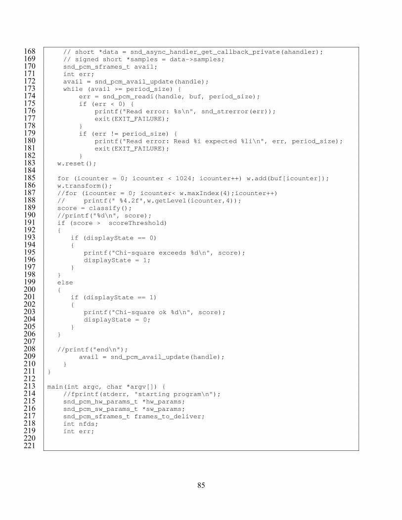
168 // short *data = snd_async_handler_get_callback_private(ahandler); 169 // signed short *samples = data->samples; 170 snd_pcm_sframes_t avail;

int err; 171 ate(handle); 172 avail = snd_pcm_avail_upd

while (avail >= period_size) { 173 eriod_size); 174 err = snd_pcm_readi(handle, buf, p

if (err < 0) { 175 )); 176 printf("Read error: %s\n", snd_strerror(err

177 exit(EXIT_FAILURE); } 178

{ if (err != period_size) 179 d %i expected %li\n", err, period_size); 180 printf("Read error: Rea

181 exit(EXIT_FAILURE); 182 } 183 w.reset(); 184 185 for (icounter = 0; icounter < 1024; icounter++) w.add(buf[icounter]); 186 w.transform(); 187 //for (icounter = 0; icounter< w.maxIndex(4);icounter++) 188 // printf(" %4.2f",w.getLevel(icounter,4)); 189 score = classify();

//printf("%d\n", score); 190 ) 191 if (score > scoreThreshold

192 { 193 if (displayState == 0) 194 { 195 printf("Chi-square exceeds %d\n", score); 196 displayState = 1; 197 } 198 } 199 else 200 { 201 if (displayState == 1) 202 { 203 printf("Chi-square ok %d\n", score); 204 displayState = 0; 205 } 206 }

207 intf("end\n"); //pr208

avail_update(handle); 209 avail = snd_pcm_210 } 211 }

212 in(int argc, char *argv[]) { ma213

program\n"); 214 //fprintf(stderr, "starting 215 snd_pcm_hw_params_t *hw_params;

snd_pcm_sw_params_t *sw_params; 216 er; 217 snd_pcm_sframes_t frames_to_deliv

218 int nfds; 219 int err; 220 221

85

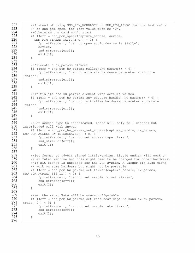
222 //Instead of using SND_PCM_NONBLOCK or SND_PCM_ASYNC for the last value 223 // of snd_pcm_open, the last value must be "0". 224 //Otherwise the card won't start 225 if ((err = snd_pcm_open(&capture_handle, device, 226 SND_PCM_STREAM_CAPTURE,0)) < 0) { 227 fprintf(stderr, "cannot open audio device %s (%s)\n", 228 device, 229 snd_strerror(err)); 230 exit(1); 231 } 232 233 //Allocate a hw_params element 234 if ((err = snd_pcm_hw_params_malloc(&hw_params)) < 0) { 235 fprintf(stderr, "cannot allocate hardware parameter structure 236 (%s)\n", 237 snd_strerror(err)); 238 exit(1); 239 } 240 241 //Initialize the hw_params element with default values. 242 if ((err = snd_pcm_hw_params_any(capture_handle, hw_params)) < 0) { 243 fprintf(stderr, "cannot initialize hardware parameter structure 244 (%s)\n", 245 snd_strerror(err)); 246 exit(1); 247 } 248 249 //Set access type to interleaved. There will only be 1 channel but 250 interleaved will work anyway 251 if ((err = snd_pcm_hw_params_set_access(capture_handle, hw_params, 252 SND_PCM_ACCESS_RW_INTERLEAVED)) < 0) { 253 fprintf(stderr, "cannot set access type (%s)\n", 254 snd_strerror(err)); 255 exit(1); 256 } 257 258 //Set format to 16-bit signed little-endian. Little endian will work on 259 // an Intel machine but this might need to be changed for other hardware. 260 //16-bit signed is expected for the DSP system. A larger bit size might 261 // work on some hardware but might not be portable 262 if ((err = snd_pcm_hw_params_set_format(capture_handle, hw_params, 263 SND_PCM_FORMAT_S16_LE)) < 0) { 264 fprintf(stderr, "cannot set sample format (%s)\n", 265 snd_strerror(err)); 266 exit(1); 267 } 268 269 //set the rate. Rate will be user-configurable 270 if ((err = snd_pcm_hw_params_set_rate_near(capture_handle, hw_params, 271 &rate, 0)) < 0) { 272 fprintf(stderr, "cannot set sample rate (%s)\n", 273 snd_strerror(err)); 274 exit(1); 275 } 276

86

277 //Set the number of channels to 1. Only one channel will be analyzed. 278 if ((err = snd_pcm_hw_params_set_channels(capture_handle, hw_params, 1)) 279 < 0) { 280 fprintf(stderr, "cannot set channel count (%s)\n", 281 snd_strerror(err)); 282 exit(1); 283 } 284 285 //Set the above specified paramters 286 if ((err = snd_pcm_hw_params(capture_handle, hw_params)) < 0) { 287 fprintf(stderr, "cannot set parameters (%s)\n", 288 snd_strerror(err)); 289 exit(1); 290 } 291 292 snd_pcm_hw_params_free(hw_params); 293 294 /* tell ALSA to wake us up whenever 1024 or more frames 295 of playback data can be delivered. Also, tell 296 ALSA that we'll start the device ourselves. 297 */ 298 299 //Allocate space for a sw_params data element 300 if ((err = snd_pcm_sw_params_malloc(&sw_params)) < 0) { 301 fprintf(stderr, "cannot allocate software parameters structure 302 (%s)\n", 303 snd_strerror(err)); 304 exit(1); 305 } 306 //snd_pcm_sw_params_current initializes sw_params with current software 307 settings 308 if ((err = snd_pcm_sw_params_current(capture_handle, sw_params)) < 0) { 309 fprintf(stderr, "cannot initialize software parameters structure 310 (%s)\n", 311 snd_strerror(err)); 312 exit(1); 313 } 314 //Set avail min inside a software configuration container. 315 //Sets Minimum avail frames to consider PCM ready, 1024 316 if ((err = snd_pcm_sw_params_set_avail_min(capture_handle, sw_params, 317 1024)) < 0) { 318 fprintf(stderr, "cannot set minimum available count (%s)\n", 319 snd_strerror(err)); 320 exit(1); 321 } 322 323 //Sets start threshold in frames. 0 in this case. 324 //PCM is automatically started when playback frames available to PCM are 325 >= threshold 326 //or when requested capture frames are >= threshold 327 if ((err = snd_pcm_sw_params_set_start_threshold(capture_handle, 328 sw_params, 0)) < 0) { 329 fprintf(stderr, "cannot set start mode (%s)\n", 330 snd_strerror(err)); 331 exit(1); 332 }

87

333 //Install PCM software configuration defined by params. 334 if ((err = snd_pcm_sw_params(capture_handle, sw_params)) < 0) { 335 fprintf(stderr, "cannot set software parameters (%s)\n", 336 snd_strerror(err)); 337 exit(1); 338 } 339 340 /* the interface will interrupt the kernel every 1024 frames, and ALSA 341 will wake up this program very soon after that. 342 */ 343 344 //Prepare PCM for use. 345 if ((err = snd_pcm_prepare(capture_handle)) < 0) { 346 fprintf(stderr, "cannot prepare audio interface for use (%s)\n", 347 snd_strerror(err)); 348 exit(1); 349 } 350 351 //struct async_private_data data; 352 snd_async_handler_t *ahandler; 353 int count; 354 355 period_size = 1024; 356 //printf("setting up callback\n"); 357 err = snd_async_add_pcm_handler(&ahandler, capture_handle, 358 async_callback, &buf); 359 if (err < 0) { 360 printf("Unable to register async handler\n"); 361 exit(EXIT_FAILURE); 362 } 363 364 err = snd_pcm_start(capture_handle); 365 if (err < 0) { 366 printf("Start error: %s\n", snd_strerror(err)); 367 exit(EXIT_FAILURE); 368 } 369 370 //open output file 371 //fout.open("D4Output.txt", ios::out); //uncomment to export data to file 372 373 //display copyright notice 374 printf("SonMon, Copyright (C) 2005 Robert Henry\n SonMon comes with 375 ABSOLUTELY NO WARRANTY;\n This is free software, and you are welcome\n to 376 redistribute it under certain conditions;\n See copy file for details.\n\n"); 377 378 /* because all other work is done in the signal handler, 379 * suspend the process */ 380 381 while (1) { 382 sleep(1); 383 } 384

88

385 printf(debugstring); 386 snd_pcm_close(capture_handle); 387 //fout.close(); //uncomment if exporting to a file. 388 exit(0); 389 }

89

1

2

Makefile

A simple make file for use in Linux to build the system

3 all: sonmon 4 5 sonmon: sonmon.o D4.o 6 g++ sonmon.o D4.o -lasound -o sonmon 7 8 D4.o: D4.cpp 9 g++ D4.cpp -c

10 11 sonmon.o: sonmon.c 12 g++ sonmon.c -c

90

1

2

3

d4dll.cpp

Builds the wavelet into a DLL suitable for use with the mathematics analysis application

Maple.

4 /* 5 Programmer: Robert K. Henry 6 Project: D4 7 Date created: 12/4/2004 8 Last modified: 8/2/2005 9 Purpose: Interface the D4 wavelet to DLL for Maple

10 Description: 11 Data are supplied in the array input. Input is fixed at 1024 12 elements. The input array MUST be defined in Maple as a c_order 13 array in row-major order. Maple arrays default to Fortran_order 14 or column-major order. In a 1-dimensional array the two 15 configurations will be the same. The output array MUST be 16 declared in Maple using the Maple C_order option. 17 18 The DLL copies the data to the wavelet class and invokes the 19 transform function. The resulting transform is returned in the 20 two-dimensional array "output". Like the input array, this array 21 must also be a C-style row-major order array and is pre-defined in 22 Maple. The array must be 512x10 but only half these elements will 23 be used since the output array is triangular. 24 25 Compiling: 26 to compile with Microsoft VC++, first set the environment variables with 27 vcvars32.bat 28 29 Then invoke the compiler with 30 cl d4dll.cpp D4.cpp -Gz -LD -link -export:d44Maple 31 32 Using in Maple: 33 The DLL must be declared in Maple. This can be done with: 34 > d4_CTrans := 35 > define_external("d44Maple", LIB="d4trans.dll", 36 > input::ARRAY(1..1024,float[8]), 37 > output::ARRAY(1..512,1..10,float[8])): 38 39 where the name of the DLL is "d4trans.dll" 40 41 The output array MUST be declared as C_order like this: 42 d1C:=Matrix(1..10,1..512,datatype=float[8],order=C_order): 43 */ 44 #include "D4.h" 45 46 __declspec(dllexport) void d44Maple( double input[1024], double 47 output[10][512]) 48 { 49 // it is assumed that the input array is 1024 50 // and the output array is 10 x 512 51 52 int i, level; 53 double t;

91

54 d4 h; 55 h.reset(); // to make sure the object starts fresh each time 56 57 for( i = 0; i < 1024; i++ ) h.add(input[i]); 58 59 h.transform(); 60 61 for( level = 0; level < 10; level++){ 62 for( i = 0; i < h.maxIndex(level); i++){ 63 t = h.getLevelSq(i, level); 64 //output[level+i*10] = t; 65 output[level][i] = t; 66 } 67 } 68 }

92

Appendix C: Gnu General Public License

Version 2, June 1991 Copyright (C) 1989, 1991 Free Software Foundation, Inc. 51 Franklin Street, Fifth Floor, Boston, MA 02110-1301, USA Everyone is permitted to copy and distribute verbatim copies of this license document, but changing it is not allowed. Preamble

The licenses for most software are designed to take away your freedom to share and change it. By contrast, the GNU General Public License is intended to guarantee your freedom to share and change free software--to make sure the software is free for all its users. This General Public License applies to most of the Free Software Foundation's software and to any other program whose authors commit to using it. (Some other Free Software Foundation software is covered by the GNU Lesser General Public License instead.) You can apply it to your programs, too. When we speak of free software, we are referring to freedom, not price. Our General Public Licenses are designed to make sure that you have the freedom to distribute copies of free software (and charge for this service if you wish), that you receive source code or can get it if you want it, that you can change the software or use pieces of it in new free programs; and that you know you can do these things. To protect your rights, we need to make restrictions that forbid anyone to deny you these rights or to ask you to surrender the rights. These restrictions translate to certain responsibilities for you if you distribute copies of the software, or if you modify it. For example, if you distribute copies of such a program, whether gratis or for a fee, you must give the recipients all the rights that you have. You must make sure that they, too, receive or can get the source code. And you must show them these terms so they know their rights. We protect your rights with two steps: (1) copyright the software, and (2) offer you this license which gives you legal permission to copy, distribute and/or modify the software. Also, for each author's protection and ours, we want to make certain that everyone understands that there is no warranty for this free software. If the software is modified by someone else and passed on, we want its recipients to know that what they have is not the original, so that any problems introduced by others will not reflect on the original authors' reputations. Finally, any free program is threatened constantly by software patents. We wish to avoid the danger that redistributors of a free program will individually obtain patent licenses, in effect making the program proprietary. To prevent this, we have made it clear that any patent must be licensed for everyone's free use or not licensed at all.

93

The precise terms and conditions for copying, distribution and modification follow. TERMS AND CONDITIONS FOR COPYING, DISTRIBUTION AND MODIFICATION

0. This License applies to any program or other work which contains a notice placed by the copyright holder saying it may be distributed under the terms of this General Public License. The "Program", below, refers to any such program or work, and a "work based on the Program" means either the Program or any derivative work under copyright law: that is to say, a work containing the Program or a portion of it, either verbatim or with modifications and/or translated into another language. (Hereinafter, translation is included without limitation in the term "modification".) Each licensee is addressed as "you". Activities other than copying, distribution and modification are not covered by this License; they are outside its scope. The act of running the Program is not restricted, and the output from the Program is covered only if its contents constitute a work based on the Program (independent of having been made by running the Program). Whether that is true depends on what the Program does. 1. You may copy and distribute verbatim copies of the Program's source code as you receive it, in any medium, provided that you conspicuously and appropriately publish on each copy an appropriate copyright notice and disclaimer of warranty; keep intact all the notices that refer to this License and to the absence of any warranty; and give any other recipients of the Program a copy of this License along with the Program. You may charge a fee for the physical act of transferring a copy, and you may at your option offer warranty protection in exchange for a fee. 2. You may modify your copy or copies of the Program or any portion of it, thus forming a work based on the Program, and copy and distribute such modifications or work under the terms of Section 1 above, provided that you also meet all of these conditions: a) You must cause the modified files to carry prominent notices stating that you changed the files and the date of any change. b) You must cause any work that you distribute or publish, that in whole or in part contains or is derived from the Program or any part thereof, to be licensed as a whole at no charge to all third parties under the terms of this License. c) If the modified program normally reads commands interactively when run, you must cause it, when started running for such interactive use in the most ordinary way, to print or display an announcement including an appropriate copyright notice and a notice that there is no warranty (or else, saying that you provide a warranty) and that users may redistribute the program under these conditions, and telling the user how to view a copy of this License. (Exception: if the Program itself is interactive but does not normally print such an announcement, your work based on the Program is not required to print an announcement.)

94

These requirements apply to the modified work as a whole. If identifiable sections of that work are not derived from the Program, and can be reasonably considered independent and separate works in themselves, then this License, and its terms, do not apply to those sections when you distribute them as separate works. But when you distribute the same sections as part of a whole which is a work based on the Program, the distribution of the whole must be on the terms of this License, whose permissions for other licensees extend to the entire whole, and thus to each and every part regardless of who wrote it. Thus, it is not the intent of this section to claim rights or contest your rights to work written entirely by you; rather, the intent is to exercise the right to control the distribution of derivative or collective works based on the Program. In addition, mere aggregation of another work not based on the Program with the Program (or with a work based on the Program) on a volume of a storage or distribution medium does not bring the other work under the scope of this License. 3. You may copy and distribute the Program (or a work based on it, under Section 2) in object code or executable form under the terms of Sections 1 and 2 above provided that you also do one of the following: a) Accompany it with the complete corresponding machine-readable source code, which must be distributed under the terms of Sections 1 and 2 above on a medium customarily used for software interchange; or, b) Accompany it with a written offer, valid for at least three years, to give any third party, for a charge no more than your cost of physically performing source distribution, a complete machine-readable copy of the corresponding source code, to be distributed under the terms of Sections 1 and 2 above on a medium customarily used for software interchange; or, c) Accompany it with the information you received as to the offer to distribute corresponding source code. (This alternative is allowed only for noncommercial distribution and only if you received the program in object code or executable form with such an offer, in accord with Subsection b above.) The source code for a work means the preferred form of the work for making modifications to it. For an executable work, complete source code means all the source code for all modules it contains, plus any associated interface definition files, plus the scripts used to control compilation and installation of the executable. However, as a special exception, the source code distributed need not include anything that is normally distributed (in either source or binary form) with the major components (compiler, kernel, and so on) of the operating system on which the executable runs, unless that component itself accompanies the executable. If distribution of executable or object code is made by offering access to copy from a designated place, then offering equivalent access to copy the source code from the same place counts as distribution of the source code, even though third parties are not compelled to copy the source along with the object code. 4. You may not copy, modify, sublicense, or distribute the Program except as expressly provided under this License. Any attempt otherwise to copy, modify, sublicense or distribute the Program is void, and will automatically terminate your rights under this License. However, parties who have received copies, or rights, from you under this License will not have their licenses terminated so long as such parties remain in full compliance.

95

5. You are not required to accept this License, since you have not signed it. However, nothing else grants you permission to modify or distribute the Program or its derivative works. These actions are prohibited by law if you do not accept this License. Therefore, by modifying or distributing the Program (or any work based on the Program), you indicate your acceptance of this License to do so, and all its terms and conditions for copying, distributing or modifying the Program or works based on it. 6. Each time you redistribute the Program (or any work based on the Program), the recipient automatically receives a license from the original licensor to copy, distribute or modify the Program subject to these terms and conditions. You may not impose any further restrictions on the recipients' exercise of the rights granted herein. You are not responsible for enforcing compliance by third parties to this License. 7. If, as a consequence of a court judgment or allegation of patent infringement or for any other reason (not limited to patent issues), conditions are imposed on you (whether by court order, agreement or otherwise) that contradict the conditions of this License, they do not excuse you from the conditions of this License. If you cannot distribute so as to satisfy simultaneously your obligations under this License and any other pertinent obligations, then as a consequence you may not distribute the Program at all. For example, if a patent license would not permit royalty-free redistribution of the Program by all those who receive copies directly or indirectly through you, then the only way you could satisfy both it and this License would be to refrain entirely from distribution of the Program. If any portion of this section is held invalid or unenforceable under any particular circumstance, the balance of the section is intended to apply and the section as a whole is intended to apply in other circumstances. It is not the purpose of this section to induce you to infringe any patents or other property right claims or to contest validity of any such claims; this section has the sole purpose of protecting the integrity of the free software distribution system, which is implemented by public license practices. Many people have made generous contributions to the wide range of software distributed through that system in reliance on consistent application of that system; it is up to the author/donor to decide if he or she is willing to distribute software through any other system and a licensee cannot impose that choice. This section is intended to make thoroughly clear what is believed to be a consequence of the rest of this License. 8. If the distribution and/or use of the Program is restricted in certain countries either by patents or by copyrighted interfaces, the original copyright holder who places the Program under this License may add an explicit geographical distribution limitation excluding those countries, so that distribution is permitted only in or among countries not thus excluded. In such case, this License incorporates the limitation as if written in the body of this License. 9. The Free Software Foundation may publish revised and/or new versions of the General Public License from time to time. Such new versions will be similar in spirit to the present version, but may differ in detail to address new problems or concerns.

96

Each version is given a distinguishing version number. If the Program specifies a version number of this License which applies to it and "any later version", you have the option of following the terms and conditions either of that version or of any later version published by the Free Software Foundation. If the Program does not specify a version number of this License, you may choose any version ever published by the Free Software Foundation. 10. If you wish to incorporate parts of the Program into other free programs whose distribution conditions are different, write to the author to ask for permission. For software which is copyrighted by the Free Software Foundation, write to the Free Software Foundation; we sometimes make exceptions for this. Our decision will be guided by the two goals of preserving the free status of all derivatives of our free software and of promoting the sharing and reuse of software generally. NO WARRANTY 11. BECAUSE THE PROGRAM IS LICENSED FREE OF CHARGE, THERE IS NO WARRANTY FOR THE PROGRAM, TO THE EXTENT PERMITTED BY APPLICABLE LAW. EXCEPT WHEN OTHERWISE STATED IN WRITING THE COPYRIGHT HOLDERS AND/OR OTHER PARTIES PROVIDE THE PROGRAM "AS IS" WITHOUT WARRANTY OF ANY KIND, EITHER EXPRESSED OR IMPLIED, INCLUDING, BUT NOT LIMITED TO, THE IMPLIED WARRANTIES OF MERCHANTABILITY AND FITNESS FOR A PARTICULAR PURPOSE. THE ENTIRE RISK AS TO THE QUALITY AND PERFORMANCE OF THE PROGRAM IS WITH YOU. SHOULD THE PROGRAM PROVE DEFECTIVE, YOU ASSUME THE COST OF ALL NECESSARY SERVICING, REPAIR OR CORRECTION. 12. IN NO EVENT UNLESS REQUIRED BY APPLICABLE LAW OR AGREED TO IN WRITING WILL ANY COPYRIGHT HOLDER, OR ANY OTHER PARTY WHO MAY MODIFY AND/OR REDISTRIBUTE THE PROGRAM AS PERMITTED ABOVE, BE LIABLE TO YOU FOR DAMAGES, INCLUDING ANY GENERAL, SPECIAL, INCIDENTAL OR CONSEQUENTIAL DAMAGES ARISING OUT OF THE USE OR INABILITY TO USE THE PROGRAM (INCLUDING BUT NOT LIMITED TO LOSS OF DATA OR DATA BEING RENDERED INACCURATE OR LOSSES SUSTAINED BY YOU OR THIRD PARTIES OR A FAILURE OF THE PROGRAM TO OPERATE WITH ANY OTHER PROGRAMS), EVEN IF SUCH HOLDER OR OTHER PARTY HAS BEEN ADVISED OF THE POSSIBILITY OF SUCH DAMAGES. END OF TERMS AND CONDITIONS

97

Appendix D: Results Summary

Threshold

1000 Threshold

900

Manu- facturer Drive ID

S.M.A.R.T. Results

Tot

al

Fram

es

Err

or

Cou

nt

% Err

or

Cou

nt

% Connor CA905DG No Response 969 2 0.21 13 1.34 IBM TVLF1297 No Response 883 1 0.11 18 2.04 Maxtor 00990202-19661-76P-H2UH No Response 1047 2 0.19 2 0.19 Maxtor A348F6VCDA43A No S.M.A.R.T. 1002 154 15.37 264 26.35

Maxtor E40AR3LA FAILED Seek_Error_Rate 744 20 2.69 99 13.31

Maxtor E40BFG9A No Response 981 981 100 981 100 Maxtor K309T6JA Passed 905 0 - 0 - Maxtor K607NJ1A Passed 793 0 - 0 - Maxtor L306XGDA No S.M.A.R.T. 967 18 1.86 48 4.96 Maxtor T1RNZVFC No Response 948 0 - 1 0.11 Maxtor W40S52VA Passed 837 0 - 0 - Quantum 79112173912 No Response 1008 0 - 1 0.10 Quantum 97X1802B No Response 1099 40 3.64 54 4.91 Quantum SG-035NTD-12547-15E-15RG Passed 838 1 0.12 1 0.12 Western Digital WM 342 197 3562 No Response 1072 382 35.63 530 49.44 Western Digital WM 356 043 2191 Passed 977 4 0.41 21 2.15 Western Digital WM 361 044 2859

FAILED Raw_Read_Error_Rate 663 0 - 3 0.45

Western Digital WM 361 214 3523 No S.M.A.R.T. 711 0 - 1 0.14 Western Digital WM 408 031 9718 Passed 1318 1 0.08 2 0.15 Western Digital WM 408 032 8026 No Response 583 297 50.94 351 60.21 Western Digital WM 408 071 0209

Passed—history of Raw_Read_Error_Rate 674 2 0.30 17 2.52

Western Digital WM 627 362 1072 Passed 879 5 0.57 25 2.84 Western Digital WM 627 362 7493 Passed 922 0 - 3 0.33 Western Digital WS 342 200 0122 No S.M.A.R.T. 1357 325 23.95 412 30.36 Western Digital WT 336 017 2647 Passed 659 0 - 4 0.61 Western Digital WT 359 004 9279 No Response 858 3 0.35 75 8.74

98

Threshold

1000 Threshold

900

Manu- facturer Drive ID

S.M.A.R.T. Results

Tot

al

Fram

es

Err

or

Cou

nt

% Err

or

Cou

nt

% Western Digital WT 364 105 0014 No Response 708 0 - 0 - Western Digital WT 473 311 2127 No S.M.A.R.T. 797 2 0.25 16 2.01 Western Digital WT 473 311 6705 Passed 942 0 - 0 -

99

VITA

ROBERT K. HENRY

Personal Data: Date of Birth: December 6, 1953 Place of Birth: Kingsport, Tennessee Marital Status: Single Education: Public Schools, Kingsport, Tennessee East Tennessee State University, Johnson City, Tennessee;

Business Administration, B.S. 1976 East Tennessee State University, Johnson City, Tennessee;

Computer Science, B.S. 2003 East Tennessee State University, Johnson City, Tennessee;

Computer Science, M.S. 2005 Professional Experience: Partner, Jo Henry Publications, 1976-2003 Graduate Assistant, East Tennessee State University,

College of Business and Technology, 2003-2005 Publications: Henry, Robert K. (2005), “Using Sound to Analyze Hardware Operation: A

Progress Report,” Proceedings of MASPLAS’05, Mid-Atlantic Student Workshop on Programming Languages and Systems, University of Delaware, April 30, 2005. 7.1-7.4

Henry, Robert K. (2005, October), Using Sound to Detect Hard Disk Failure, Poster presentation at SASPLAS 2005, Southern Appalachian Symposium for Programming Languages and Systems.

Honors and Awards: Summa cum laude Kappa Mu Epsilon Phi Kappa Phi Upsilon Pi Epsilon

100