Monitoring of retrievals from the MIPAS and SCIAMACHY ...

ESA Contract Report

Contract Report to the European Space Agency

Monitoring of retrievals from the MIPAS and SCIAMACHY instruments on board ENVISAT

December 2003

Author: Antje Dethof Final report for ESA contract 14458/00/NL/SF: Technical Support for global validation of ENVISAT data products

Series: ECMWF - ESA Contract Report A full list of ECMWF Publications can be found on our web site under: http://www.ecmwf.int/publications/ Contact: [email protected] © Copyright 2003 European Centre for Medium Range Weather Forecasts Shinfield Park, Reading, RG2 9AX, England Literary and scientific copyrights belong to ECMWF and are reserved in all countries. This publication is not to be reprinted or translated in whole or in part without the written permission of the Director. Appropriate non-commercial use will normally be granted under the condition that reference is made to ECMWF. The information within this publication is given in good faith and considered to be true, but ECMWF accepts no liability for error, omission and for loss or damage arising from its use.

http://www.ecmwf.int/publications/



Monitoring of retrievals from the MIPAS and SCIAMACHY instruments on board ENVISAT

Author: Antje Dethof

Final report for ESA contract 14458/00/NL/SF: Technical Support for global validation of

ENVISAT data products

European Centre for Medium-Range Weather Forecasts Shinfield Park, Reading, Berkshire, UK

December 2003

Monitoring of MIPAS and SCIAMACHY retrievals at ECMWF

Abstract

Contracted by ESA, ECMWF is involved in the validation and monitoring of atmospheric data from severalinstruments on board ENVISAT. Under contract 14458/00/NL/SF (Technical support for global validation ofENVISAT data products), which ran from 1.4.2000 to 30.9.2003, ECMWF monitored near-real-time Level2 data products from SCIAMACHY, MIPAS and GOMOS. During the first part of the contract, a monitoringframework for these ENVISAT data was developed at ECMWF. During the second part of the contract, thetools that had been developed were used to monitor and validate the ENVISAT data. This paper is the finalreport for ESA contract 14458/00/NL/SF and describes results from the monitoring statistics of MIPAS andSCIAMACHY data.

1 Introduction

ESA’s ENVISAT (Environmental Satellite) was launched on 1 March 2002. On board are several instrumentsthat allow the retrieval of profiles or total column values of various atmospheric constituents. One of theseinstruments is SCIAMACHY (Scanning Imaging Absorption Spectrometer for Atmospheric CHartographY),a spectrometer that measures backscattered, reflected, transmitted or emitted radiation from the atmosphereand the Earth’s surface in the wavelength region 240-2380 nm at moderate spectral resolution (0.2 nm - 1.5nm). The instrument has three viewing modes: limb, nadir and occultation, and its prime objective is toprovide global measurements of various trace gases in the troposphere and stratosphere (including O3, NO2,BrO, OClO, SO2 and H2CO), as well as the determination of aerosols and clouds. The second instrument isMIPAS (Michelson Interferometer for Passive Atmospheric Sounding), a limb-viewing high-resolution Fourier-transform spectrometer that measures atmospheric emissions in the mid infrared part of the spectrum (4.15microns to 14.6 microns), allowing the retrieval of concentration profiles of more than 20 atmospheric tracegases, from 70 km down to 7 km, with a vertical resolution of 3-5 km. MIPAS provides global coverage,including coverage of the polar regions, independent of illumination conditions. The six main species (O3,H2O, HNO3, CH4, N2O and NO2) as well as temperature and pressure profiles are routinely retrieved by theESA ground segment. The third instrument is GOMOS (Global Ozone Monitoring by Occultation of Stars)that makes use of the occultation measurement principle by tracking stars as they set behind the atmosphere.GOMOS has an UV-visible and a near-infrared spectrometer, covering the wavelength region 250-950 nm. Itallows the retrieval of atmospheric trace gas profiles in the altitude range 100-20 km, with an altitude resolutionbetter than 1.7 km. GOMOS gives day- and night time measurements with about 600 profiles per day. Theprimary GOMOS target species are O3, NO2, NO3, OClO, H2O and temperature.

ECMWF is contracted by ESA (project 14458/00/NL/SF) to give technical support for the global valida-tion of ENVISAT data products. This includes the monitoring and validation of a subset of the ENVISATlevel 2 retrievals, the so called Meteo products, which are available in near-real-time (NRT) in BUFR for-mat. These Meteo data include temperature, ozone and water vapour profiles from MIPAS (MIP NLE 2P) andGOMOS (GOM RR 2P), as well as SCIAMACHY total column ozone data from from nadir measurements(SCI RV 2P).

The ECMWF model is a global spectral model with a horizontal truncation of T511 (about 40 km grid spacing).The model has 60 levels in the vertical and the model top is at 0.1 hPa (corresponding to about 65 km). Theoperational model uses a 4-dimensional variational analysis scheme (Rabier et al. 2000), to assimilate observa-tions at 12 hourly intervals. The 4D-Var data assimilation works in the following way: A first-guess trajectoryis calculated by running the model for 12 hours. During this forecast the differences between the model andthe observations are being recorded. A minimization run is then carried out with the tangent linear and adjointmodels. During this minimization the differences between model and observations are transported back in timeto the start of the forecast in order to derive a corrected state for a model run within the time window. From this

ESA report 1


improved state a new forecast is run. At ECMWF two trajectory runs and two minimizations are carried out ineach assimilation cycle. The first minimization uses a simplified parameterization of the physical processes inthe atmosphere and is run at the lower resolution of T95, the second one uses a more comprehensive physicspackage and is run at the resolution of T159.

Because ozone is fully integrated into the ECMWF forecast model and analysis system (Dethof and Holm2003) as an additional three-dimensional model and analysis variable, the ECMWF model can be used tomonitor ozone retrievals from the ENVISAT instruments in addition to temperature and water vapour. Theforecast model includes a simple ozone parameterization, which is an updated version ofCariolle and Deque( 1986). The ECMWF ozone parameterization includes an additional term which parameterizes the depletion ofozone in polar regions by heterogeneous reactions. At present, ozone is included uni-variately in the ECMWFdata assimilation system. This means that there are no ozone increments from the analysis of the dynamicalfields, even though the assimilation of ozone observations will modify the wind field in 4D-Var through theadjoint calculations. The univariate treatment was chosen to minimize the effect of ozone on the rest of theanalysis system. For the same reason, the model’s ozone field is not used in the radiation scheme, where anozone climatology (Fortuin and Langematz 1995) is used instead.

Ozone retrievals from the SBUV/2 (Solar Backscatter Ultra Violet) instrument on NOAA-16 have been as-similated in the operational ECMWF system since April 2002. The SBUV/2 data come from NESDIS (seehttp://orbit-net.nesdis.noaa.gov/crad/sit/ozone/ for more information). They are given as 12 ozone layers andare combined at ECMWF into 6 ozone layers (0.1-1 hPa, 1-2 hPa, 2-4 hPa, 4-8 hPa, 8-16 hPa, 16 hPa-surface)to reduce observation error correlation. Between April 2002 and June 2003, total column ozone retrievals fromthe GOME (Global Ozone Monitoring Experiment) instrument on ERS-2 were also assimilated operationally.The GOME retrievals were the NRT total column data produced by KNMI’s fast delivery service, version FD3.1 (Valks et al. 2003). The ozone data are used in the following way. GOME data are only used at solarzenith angles less than 80Æ and at latitudes between 40ÆN and 50ÆS. This conservative approach was chosenbecause the bias between the GOME data and the model can be large outside this latitude band, and we wantedto minimize the impact of the ozone assimilation on the rest of the assimilation system. The SBUV/2 data arenot used at solar zenith angles greater than 84Æ. Variational quality control and first-guess checks are carriedout for both datasets.

In the ECMWF analysis system no humidity observations are assimilated in the stratosphere. A simple pa-rameterization of the upper-stratospheric moisture source due to methane oxidation is included to avoid anunrealistically drying of the stratosphere in the ECMWF model (Simmons pers. comm.). Stratospheric hu-midity values from the 45-year re-analysis project (ERA-40) are about 10-15% lower than UARS retrievals inthe upper stratosphere and lower mesosphere at high latitudes where air moistened by methane oxidation hasdescended. Since then, the parameterization of methane oxidation has been modified to take into account amore recent climatology of methane, so that the dry bias of the current operational ECMWF model should besmaller than in ERA-40. In the lower stratosphere the ECMWF water vapour field shows a too rapid upwardprogression of the annual cycle of drying and moistening in the tropics.

Satellite data can be monitored with the help of a data assimilation system by looking at the differences betweenthe observations and collocated model fields. The model fields are interpolated in time and space to the locationof the observations, statistical analyses of the differences between the model’s first-guess or analysed fields andthe observations are calculated, and their time evolution is monitored. The differences between the observationsand the model fields are called departures. We distinguish between first-guess departures (observations minusfirst-guess field) and analysis departures (observations minus analysed field). If the model fields are stable thedepartures normally show a relatively smooth behaviour from day to day. A sudden jump on a global scale,which is larger than the instrument noise, is an indication of possible problems in the data or the model. Longterm monitoring of the departures can disclose errors and biases in the satellite data products, as well as errors

2 ESA report


or biases in the model. It enables us to carry out a continuous quality assessment of the ENVISAT data. Suchlong term monitoring statistics can also detect biases between the different ENVISAT products (e.g. betweenozone retrievals from different instruments) and allows us to monitor instrument and algorithm stability. Theadvantage of using an assimilation system to monitor satellite data is that it provides continuous global coverageand that it allows one to build up statistics quickly. Furthermore, it gives a framework in which to compare thesatellite data with other sources of information, for instance radiosondes or ozone sondes, and it also helps tocharacterize the error statistics of the observations if the model error characteristics are known.

Even though ENVISAT was launched on 1 March 2002, ECMWF did not receive any data until August 2002,and even then there were problems with the data flow. During the first weeks, only parts of orbits were received.Because of problems with the delivery of the Meteo products in BUFR format, ENVISAT data in PDS formwere used and converted into BUFR format at ECMWF. Further problems with the data delivery meant thatno ENVISAT data were monitored in January 2003 and the first half of February 2003. From the middle ofFebruary 2003 onwards the data flow improved and the monitoring could continue. The quality of the NRTESA GOMOS retrievals has been poor up to now, and we are waiting for an algorithm update before monitoringthe data. Hence, GOMOS data are not discussed in this report.

At the beginning ENVISAT data were used only passively in the ECMWF assimilation system. This means thedata were fed into the system, first-guess statistics were calculated, but the data were not assimilated into theECMWF model. The assimilation of MIPAS ozone retrievals was tested in research experiments and was foundto have a positive impact on the ECMWF ozone field (Dethof 2003). It underwent pre-operational testing fromJune to October 2003 (in the CY26R3 e-suite) and has been included in the operational ECMWF system sinceOctober 2003.

The monitoring statistics shown in this paper cover the period 17 February to 5 October. They are split intotwo parts. From 17 February to 31 May 2001 ENVISAT data were monitored in off-line experiments whichused 3-dimensional variational analysis (Courtier et al. 1998) and which were run at a horizontal truncation ofT159, using CY25R4 of the ECMWF model. All ENVISAT data were passive in these experiments. From 1June to 5 October 2003, ENVISAT data were monitored in the pre-operational CY26R3 e-suite using the fullT511, 12-hour 4D-Var system. MIPAS ozone profiles were actively assimilated in CY26R3, while the otherENVISAT data were monitored passively.

This paper describes the monitoring of SCIAMACHY and MIPAS data at ECMWF. It is structured in thefollowing way. Section 2 summarizes the results of the monitoring of SCIAMACHY total column ozone data,Section 3 the results of the monitoring of MIPAS temperature, water vapour and ozone retrievals, and Section4 gives the conclusions.

2 Monitoring of NRT retrievals from SCIAMACHY (SCI RV 2P)

At ECMWF SCIAMACHY total column ozone data from nadir measurements in the UV/VIS (SCI RV 2P)are monitored. Unfortunately, these NRT Level 2 SCIAMACHY data do not include geolocation informationlike solar zenith angle or field of view which are included in the off-line Level 2 data. Consequently, data orretrieval problems related to these parameters can not be identified by monitoring the NRT data.

Figure 1 shows timeseries of zonal mean total column ozone values (averaged over 6-hourly analysis cycles)from SCIAMACHY in Dobson Units (DU) from 17 February to 30 May (top panel) and from 1 June to 5October 2003 (bottom panel). The timeseries shows the periods when no data were available. It also illustratesthat SCIAMACHY ozone values lie within a realistic range and reproduce well the seasonal cycle of totalcolumn ozone (e.g. high values in the NH during spring, the development of the Antarctic ozone hole between

ESA report 3


17FEB

19 21 23 25 27 1MAR

3 5 7 9 11 13 15 17 19 21 23 25 27 29 31 2APR

4 6 8 10 12 14 16 18 20 22 24 26 28 30 2MAY

4 6 8 10 12 14 16 18 20 22 24 26 28 30

-80-70-60-50-40-30-20-10

0102030405060708090

Latit

ude

-80-70-60-50-40-30-20-10

0102030405060708090

Latit

ude

120 – 150 150 – 180 180 – 210 210 – 240 240 – 270 270 – 300 300 – 330 330 – 360360 – 390 390 – 420 420 – 450 450 – 480 480 – 510 510 – 540 540 – 570

120 – 150 150 – 180 180 – 210 210 – 240 240 – 270 270 – 300 300 – 330 330 – 360360 – 390 390 – 420 420 – 450 450 – 480 480 – 510 510 – 540 540 – 570

1JUN

3 5 7 9 3 5 7 911131517192123252729 1JUL

1113151719212325272931 2AUG

4 6 8 1012141618202224262830 1SEP

3 5 7 9 11131517192123252729 1OCT

3 5

Figure 1: Timeseries of zonal mean SCIAMACHY total column ozone values in DU from 17 February to 30 May 2003 (top) and from1 June to 5 October 2003 (bottom).

4 ESA report


17FEB

19 21 23 25 27 1MAR

3 5 7 9 11 13 15 17 19 21 23 25 27 29 31 2APR

4 6 8 10 12 14 16 18 20 22 24 26 28 30 2MAY

4 6 8 10 12 14 16 18 20 22 24 26 28 30

-80-70-60-50-40-30-20-10

0102030405060708090

Latit

ude

120 – 150 150 – 180 180 – 210 210 – 240 240 – 270 270 – 300 300 – 330 330 – 360360 – 390 390 – 420 420 – 450 450 – 480 480 – 510 510 – 540 540 – 570

Figure 2: Timeseries of zonal mean GOME total column ozone data in DU from 17 February to 30 May 2003.

17FEB

19 21 23 25 27 1MAR

3 5 7 9 11 13 15 17 19 21 23 25 27 29 31 2APR

4 6 8 10 12 14 16 18 20 22 24 26 28 30 2MAY

4 6 8 10 12 14 16 18 20 22 24 26 28 30

-80-70-60-50-40-30-20-10

0102030405060708090

Latit

ude

–70 – –60 –60 – –50 –50 – –40 –40 – –30 –30 – –20 –20 – –10 –10 – 0 0 – 1010 – 20 20 – 30 30 – 40 40 – 50 50 – 60 60 – 70 70 – 80

Figure 3: Timeseries of zonal mean SCIAMACHY first-guess departures in DU from 17 February to 30 May 2003.

ESA report 5


August and October). However, compared to GOME total column ozone retrievals (Figure2) SCIAMACHYdata show a negative bias of about 30 DU over much of the globe. The same bias can be seen when comparingSCIAMACHY data with the ECMWF first-guess ozone field. Figure 3 shows a timeseries of zonal mean first-guess departures in % for SCIAMACHY. The SCIAMACHY data are 10-20% lower than the first-guess overmost of the globe. At the beginning of the timeseries during February and March, the negative departuresare even larger. Positive departures are seen at the northern end of the orbits in February and March, and atthe southern end of the orbits from the end of March onwards. It is possible that there are problems withSCIAMACHY retrievals at high solar zenith angles, but this can not be further investigated because there is noinformation about solar zenith angle in the NRT SCIAMACHY data.

100

200

300

400

500

600

[ DU

]

OBS FG ANA

FEB23 1 7 13 19 25 31 6 12 18 24 30 6 12 18 24

MAR APR MAY30

FEB23 1 7 13 19 25 31 6 12 18 24 30 6 12 18 24

MAR APR MAY30

-100

-60

-20

20

60

100

[ DU

]

[ DU

] [ D

U ]

OBS-FG OBS-AN

JUN5 13 21 29

JUL AUG7 15 23 31 8 16 24 1

SEP9 17 25

OCT3

JUN5 13 21 29

JUL AUG7 15 23 31 8 16 24 1

SEP9 17 25

OCT3

100

200

300

400

500

600OBS FG ANA

-100

-60

-20

20

60

100OBS-FG OBS-AN

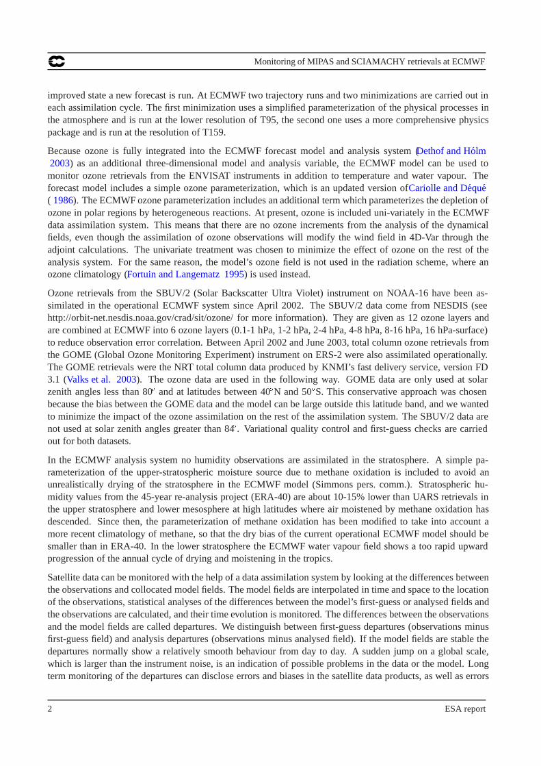
Figure 4: Timeseries of data averaged over 90-65ÆN covering the periods 17 February to 30 May (left) and 1 June to 5 October 2003(right). The top panels show SCIAMACHY observations, first-guess and analysis values, the second panels first-guess and analysisdepartures. All ozone values are in DU.

100

200

300

400

500

600

[ DU

]

OBS FG ANA

FEB23 1 7 13 19 25 31 6 12 18 24 30 6 12 18 24

MAR MAR MAY30

FEB23 1 7 13 19 25 31 6 12 18 24 30 6 12 18 24

MAR MAR MAY30

–100

–60

–20

20

60

100

[ DU

]

[ DU

] [ D

U ]

OBS-FG OBS-AN

JUN5 13 21 29

JUL AUG7 15 23 31 8 16 24 1

SEP9 17 25

OCT3

JUN5 13 21 29

JUL AUG7 15 23 31 8 16 24 1

SEP9 17 25

OCT3

100

200

300

400

500

600OBS FG ANA

–100

–60

–20

20

60

100OBS-FG OBS-AN

Figure 5: Like Figure 4 but for 30ÆN-30ÆS.

The negative bias of the SCIAMACHY data becomes even clearer when looking at timeseries of area averagedSCIAMACHY and analysis values, as well as timeseries of departures. Figure 4 shows a timeseries of dataaveraged over the area between 90-65ÆN. The observation values are systematically lower than the first-guessand analysis values. The departures are larger during February and March, and the departures as well as theobservations show a larger standard deviation then. From about 24 April onwards the standard deviation of the

6 ESA report


100

200

300

400

500

600

[ DU

]

OBS FG ANA

FEB23 1 7 13 19 25 31 6 12 18 24 30 6 12 18 24

MAR APR MAY30

FEB23 1 7 13 19 25 31 6 12 18 24 30 6 12 18 24

MAR APR MAY30

–100

–60

–20

20

60

100

[ DU

]

[ DU

] [ D

U ]

OBS-FG OBS-AN

JUN5 13 21 29

JUL AUG7 15 23 31 8 16 24 1

SEP9 17 25

OCT3

JUN5 13 21 29

JUL AUG7 15 23 31 8 16 24 1

SEP9 17 25

OCT3

100

200

300

400

500

600OBS FG ANA

–100

–60

–20

20

60

100OBS-FG OBS-AN

Figure 6: Like Figure 4 but for 65-90ÆS.

observations and departures is smaller and more stable, and SCIAMACHY data are around 30 DU lower thanthe ECMWF first-guess and analysis values.

Between 30ÆN-30ÆS (Figure 5) the observation values and the departures are more stable, with a negative biasof 25-30 DU for the whole period from February to October 2003. There is an offset during August whenSCIAMACHY values are higher than normal and departures are smaller (around 20 DU). The reason for thischange is not clear. Another offset in the departures can be seen from 6-17 September, when the analysis valuesare slightly lower than outside this period, again leading to smaller departures around 20 DU. This change isa result of an offset in MIPAS ozone retrievals assimilated at that time, which affected the ozone analysis (seeSection 3 for more details).

Between 65-90ÆS (Figure 6) the area averaged departures are less stable. The largest negative departures areseen in February and March. From May to July departures are small or even slightly positive, and from Augustonwards they are negative again. It is likely that the reason for these changes is the varying data coverage ofthe area between 65-90ÆS from February to October, with only few data going into the average between Mayand August.

The negative bias of the SCIAMACHY data seen in the timeseries plots is also apparent when plotting a his-togram of SCIAMACHY first-guess departures (Figure 7). The mean bias over the period 17 February to 30May 2003 is -30.7 DU, with a standard deviation of 16.8 DU. This figure illustrates that the bias of the SCIA-MACHY data is the main problem, and that otherwise the data seem to be well characterized with normallydistributed departures. SCIAMACHY data might be suitable for assimilation if the bias can be removed, ideallyby improving the retrieval algorithm, or otherwise by implementing a bias correction scheme for SCIAMACHYdata at ECMWF to remove the bias before the data are assimilated.

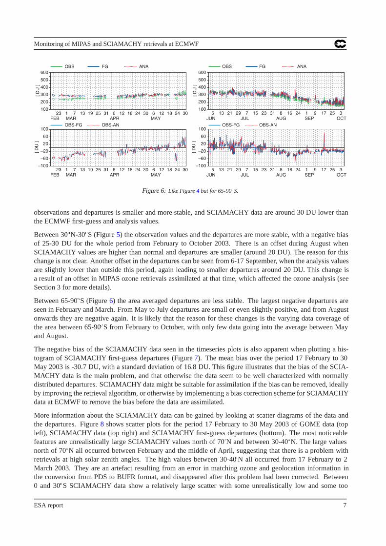
More information about the SCIAMACHY data can be gained by looking at scatter diagrams of the data andthe departures. Figure 8 shows scatter plots for the period 17 February to 30 May 2003 of GOME data (topleft), SCIAMACHY data (top right) and SCIAMACHY first-guess departures (bottom). The most noticeablefeatures are unrealistically large SCIAMACHY values north of 70ÆN and between 30-40ÆN. The large valuesnorth of 70ÆN all occurred between February and the middle of April, suggesting that there is a problem withretrievals at high solar zenith angles. The high values between 30-40ÆN all occurred from 17 February to 2March 2003. They are an artefact resulting from an error in matching ozone and geolocation information inthe conversion from PDS to BUFR format, and disappeared after this problem had been corrected. Between0 and 30ÆS SCIAMACHY data show a relatively large scatter with some unrealistically low and some too

ESA report 7


-100 -80 -60 -40 -20 0 20 40 60 80 100OBS-FG (DU)

0

0.1

0.2

0.3

0.4

0.5

0.6

0.7

0.8

0.9

1

Num

ber/

Num

ber m

ax

Figure 7: Frequency distribution of SCIAMACHY first-guess departures in DU for the period 17 February to 30 May 2003.

high ozone values. This might be a sign of cloud contamination, but because there is no information aboutcloud cover or cloud top height in the NRT SCIAMACHY data this can not be investigated further. The scatterdiagram of GOME data for the same period does not show such a large scatter between 0 and 30ÆS nor does itshow unrealistically large values north of 70ÆN. Comparing the scatter diagrams of GOME and SCIAMACHYdata again shows the negative bias of the SCIAMACHY data, which is also apparent in the scatter plot ofSCIAMACHY first-guess departures.

Figure 9 shows scatter plots of SCIAMACHY data (left) and first-guess departure (right) for 1 June to 5 October2003. The unrealistically large values north of 70ÆN are not seen any more, but there is still a large scatterbetween 0-30ÆS. The plot of the departures shows again a mean negative bias of 25-30 DU over most latitudes,but larger departures are seen at hight latitudes in both hemispheres.

In summary it can be said that there are still too many problems with the NRT SCIAMACHY data to allowtheir assimilation in the ECMWF system. The main problem is the negative bias of the data which has beenobserved and reported to ESA ever since the first data became available. A further problem is the lack ofgeolocation information in the NRT SCIAMACHY data, such as solar zenith angle, field of view, cloud topheight, or cloud cover information. This makes it impossible to attribute problems to certain parameters (e.g.cloud contamination, problems with observations at hight solar zenith angle) and makes a thorough analysis ofthe data difficult. It also makes it impossible to use a subset of the data screened according to certain criteria,for instance, to only use data below a solar zenith angle threshold actively in the assimilation.

SCIAMACHY retrievals produced by KNMI are currently being tested at ECMWF. First studies show theseretrievals to be of better quality than the ESA NRT SCIAMACHY products. The KNMI retrievals do not showa negative bias, and agree better with the ECMWF total ozone field. Furthermore, they do include geolocationinformation. The assimilation of the KNMI SCIAMACHY retrievals will be tested in research experiments.

8 ESA report


–90 –70 –50 –30 –10 10 30 50 70 90

90

Latitude [ deg ]

050

100150200250300350400450500550600650700750800850900950

1000O

BS

[ D

U ]

1251020507510020050075010002000500075001000050000

–90 –70 –50 –30 –10 10 30 50 70Latitude [ deg ]

OB

S–F

G [

DU

]

1251020507510020050075010002000500075001000050000

–90 –70 –50 –30 –10 10 30 50 70 90Latitude [ deg ]

050

100150200250300350400450500550600650700750800850900950

1000

OB

S [

DU

]

1251020507510020050075010002000500075001000050000

–200–175–150–125–100–75–50–25

0255075

100125150175200

Figure 8: Scatterplots for the period 17 February to 30 May 2003 of GOME total ozone (top left), SCIAMACHY total ozone (topright), and SCIAMACHY first-guess departures (bottom). Ozone values are in DU.

3 Monitoring of NRT temperature, water vapour and ozone retrievals fromMIPAS (MIP NLE 2P)

This section describes on the monitoring of NRT temperature, water vapour and ozone retrievals from theMIPAS instrument (MIP NLE 2P) at ECMWF.

3.1 NRT temperature retrievals from MIPAS

Figure 10 shows area averaged MIPAS and ECMWF temperature profiles for the areas 90-65ÆN (top left), 0-20ÆS (middle left) and 65-90ÆS (bottom left) averaged over the period 17 February to 30 May 2003. The rightpanels show the corresponding MIPAS departures. On the whole, MIPAS temperature profiles are of goodquality, and the differences between MIPAS and ECMWF temperatures are less than 2% (less than 4 K) formost levels. Larger departures are seen near the model top. MIPAS temperatures are larger than ECMWFtemperatures throughout the stratosphere. In the mesosphere the sign of the departures varies depending on thearea and the time of year. This leads to relatively small mean departures in 90-65ÆN and 65-90ÆS for the wholeaveraging period, but departures can be large for shorter periods, as illustrated by the large standard deviationsof the departures near the model top. MIPAS temperatures are usually lower than ECMWF temperature at0.1 hPa, with the exception of the winter pole, where the ECMWF model has a cold bias of up to 20K at themodel top.

ESA report 9


–90 –70 –50 –30 –10 10 30 50 70 90Latitude [ deg ]

050

100150200250300350400450500550600650700750800850900950

1000O

BS

[ D

U ]

1251020507510020050075010002000500075001000050000

–90 –70 –50 –30 –10 10 30 50 70 90Latitude [ deg ]

1251020507510020050075010002000500075001000050000

OB

S–F

G [

DU

]

–200–175–150–125–100–75–50–25

250

5075

100125150175200

Figure 9: Scatterplots for the period 1 June to 5 October 2003 of SCIAMACHY total ozone (left), and SCIAMACHY first-guessdepartures (right). Ozone values are in DU.

Figure 11 shows MIPAS temperature profiles and departures averaged over the period from 1 June to 5 October2003, based on results from the CY26R3 e-suite. In CY26R3 radiances from the AIRS instrument on Aquaare assimilated, which has an impact on the ECMWF temperatures in the stratosphere and mesosphere. Theprofile plots show a good agreement between MIPAS and ECMWF temperatures over most of the stratospherein 90-65ÆN and 0-20ÆS, with departures of less than 2%. MIPAS temperatures are again larger than ECMWFvalues in the stratosphere and lower near the model top. In 65-90ÆS, there are some unrealistic structures inthe ECMWF temperature profiles in the upper stratosphere and lower mesosphere. The ECMWF model has astrong cold bias over the winter pole, and problems arise when AIRS radiances are assimilated in the presenceof this bias. The AIRS data warm the model top, but the background error formulation has temperature errorsthat have anti-correlations in the vertical, and this leads to unrealistic oscillations further down the profiles whentrying to fit the AIRS radiances. These problems are an artefact of the assimilation system and not a problem inthe data. They are currently addressed by blacklisting the upper stratospheric AIRS channels. In the long termthe model’s cold bias will have to be reduced. MIPAS data were a useful independent data set to identify theseproblems.

Figures 12 to 14 show timeseries of area averaged temperatures and departures at 20 hPa for the areas 90-65ÆN, 0-20ÆS, and 65-90ÆS, respectively. The figures illustrate that MIPAS data delivery is better from Juneonwards, and that there are several data gaps between February and May 2003. The timeseries show that thearea averaged MIPAS temperatures at 20 hPa in the tropics are relative constant around 225 K throughoutthe monitoring period. In the other two areas there is a pronounced seasonal cycle. In 90-65ÆN, temperaturesincrease from values around 215-220 K in February and March, to values around 230K in April and then remainare between 230-235 K until the beginning of September, when they begin too decrease to values of 215 K bythe beginning of October. In 65-90ÆS, temperatures at 20 hPa reach minimum values of 175 K in July duringthe polar night and then increase again to values around 235 K at the beginning of October. Figure14 showsthat temperatures over the South Pole are low enough for the formation of polar stratospheric clouds (PSCs)from June to September.

MIPAS temperatures are slightly higher than ECMWF temperatures in all three areas, but departures are lessthan 2 K for most of the timeseries. The departures usually show a stable behaviour from day to day, but thereare some periods (23 February to 1 March, 20/21 March, 21 May to 10 June, 6 to 17 September) when MIPAStemperatures are 3-8 K higher than normal. These discontinuities occurred after payload or instrument switch-offs. For example, when the operation of MIPAS was resumed on 6 September, the ice deposition conditionswere different to what they had been before the cooler switch-off. However, pre-switch-off gain calibrations

10 ESA report


180 190 200 210 220 230 240 250 260 270 280 290 300Temperature [ K ]

200

10060

20

106

2

10.6

0.2

0.1

Pre

ssur

e [h

Pa]

200

10060

20

106

2

10.6

0.2

0.1

Pre

ssur

e [h

Pa]

OBSFGANAOBS+STDVOBS–STDV

–10 –8 –6 –4 –2 0 2 4 6 8 10[ %]

180 190 200 210 220 230 240 250 260 270 280 290 300Temperature [ K ]

200

10060

20

106

2

10.6

0.2

0.1

Pre

ssur

e [h

Pa]

200

10060

20

106

2

10.6

0.2

0.1

Pre

ssur

e [h

Pa]

–10 –8 –6 –4 –2 0 2 4 6 8 10[ %]

180 190 200 210 220 230 240 250 260 270 280 290 300Temperature [ K ]

200

10060

20

106

2

10.6

0.2

0.1

Pre

ssur

e [h

Pa]

200

10060

20

106

2

10.6

0.2

0.1

Pre

ssur

e [h

Pa]

–10 –8 –6 –4 –2 0 2 4 6 8 10[ %]

(OBS-FG)/FG(OBS-ANA)/ANAstdv(OBS-FG)/FGstdv(OBS-AN)/ANA

Figure 10: Profiles of time and area averaged MIPAS and ECMWF temperatures in K (left) and MIPAS departures in % (right) forthe areas 90-65ÆN (top), 0-20ÆS (middle), and 65-90ÆS (bottom). Averaging period is 17 February to 30 May 2003.

ESA report 11


180 190 200 210 220 230 240 250 260 270 280 290 300Temperature [ K ]

200

10060

20

106

2

10.6

0.2

0.1

Pre

ssur

e [h

Pa]

200

10060

20

106

2

10.6

0.2

0.1

Pre

ssur

e [h

Pa]

OBSFGANAOBS+STDVOBS–STDV

–10 –8 –6 –4 –2 0 2 4 6 8 10[ %]

180 190 200 210 220 230 240 250 260 270 280 290 300Temperature [ K ]

200

10060

20

106

2

10.6

0.2

0.1

Pre

ssur

e [h

Pa]

200

10060

20

106

2

10.6

0.2

0.1

Pre

ssur

e [h

Pa]

–10 –8 –6 –4 –2 0 2 4 6 8 10[ %]

180 190 200 210 220 230 240 250 260 270 280 290 300Temperature [ K ]

200

10060

20

106

2

10.6

0.2

0.1

Pre

ssur

e [h

Pa]

200

10060

20

106

2

10.6

0.2

0.1

Pre

ssur

e [h

Pa]

–10 –8 –6 –4 –2 0 2 4 6 8 10[ %]


Figure 11: Like Figure 10 but for 1 June to 5 October 2003.

12 ESA report


OBS-FG OBS-AN OBS-FG OBS-AN

JUN5 13 21 29

JUL AUG7 15 23 31 8 16 24 1

SEP9 17 25

OCT3

JUN5 13 21 29

JUL AUG7 15 23 31 8 16 24 1

SEP9 17 25

OCT3

160180200220240260280

[ K ]

–10

–6

–2

2

6

10

[ K ]

160180200220240260280

[ K ]

–10

–6

–2

2

6

10

[ K ]

FEB23 1 7 13 19 25 31 6 12 18 24 30 6 12 18 24

MAR APR MAY30

FEB23 1 7 13 19 25 31 6 12 18 24 30 6 12 18 24

MAR APR MAY30

OBS FG ANA OBS FG ANA

Figure 12: Timeseries of temperature data averaged over 90-65ÆN covering the periods 17 February to 30 May (left) and 1 June to5 October 2003 (right). The top panels show MIPAS temperatures, first-guess and analysis values, the second panels first-guess andanalysis departures. All temperature values are in K.

160180200220240260280

[ K ]

–10

–6

–2

2

6

10

[ K ]

160180200220240260280

[ K ]

–10

–6

–2

2

6

10

[ K ]

FEB23 1 7 13 19 25 31 6 12 18 24 30 6 12 18 24

MAR APR MAY30

FEB23 1 7 13 19 25 31 6 12 18 24 30 6 12 18 24

MAR APR MAY30



JUN5 13 21 29

JUL AUG7 15 23 31 8 16 24 1

SEP9 17 25

OCT3

JUN5 13 21 29

JUL AUG7 15 23 31 8 16 24 1

SEP9 17 25

OCT3


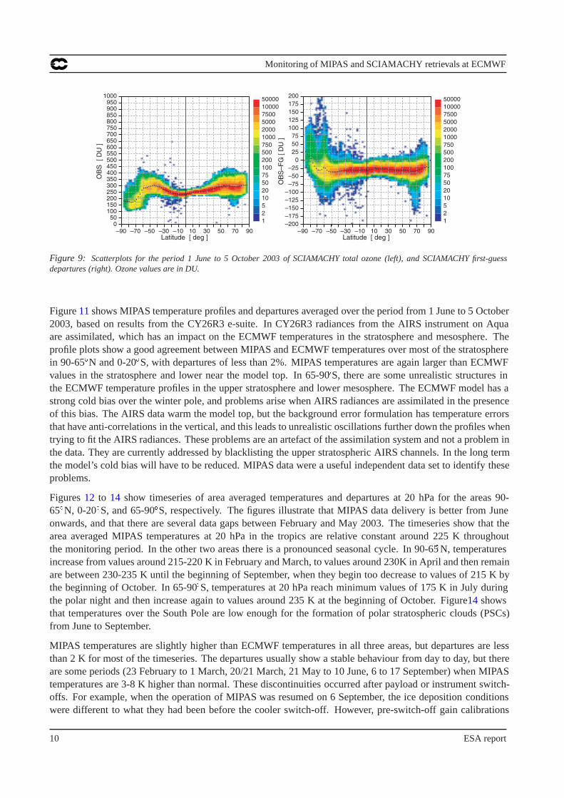
were applied to the post-switch-off data. After new gain calibrations had been performed, MIPAS values wentback to pre-switch-off levels. The offsets in the temperature retrievals propagated into the trace retrievals andcan be seen in the monitoring timeseries for MIPAS water vapour (Figures 17 to 19) and ozone retrievals(Figures 22 to 24). These timeseries illustrate the power of an assimilation system for monitoring satellite data.It allows ECMWF to quickly identify and quantify problems and give ESA feedback.

3.2 NRT water vapour retrievals from MIPAS

In the ECMWF assimilation system water vapour layers or partial columns (unit kgm�2) are monitored, notwater vapour profile points. These partial layers are calculated for MIPAS data during the conversion fromPDS to BUFR format.

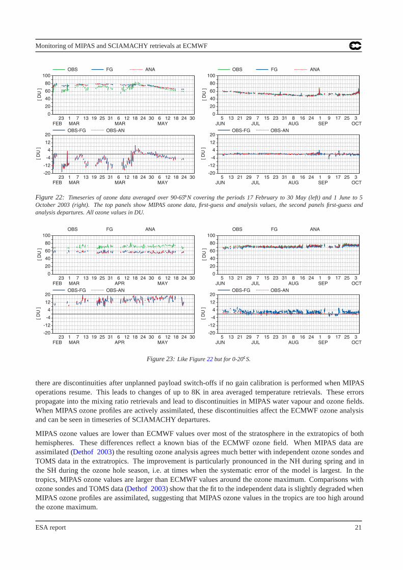
Time and area averaged MIPAS water vapour profiles and departures for the areas 90-65ÆN, 0-20ÆS, and 65-90ÆS are shown in Figure 15 averaged over the periods 17 February to 30 May (left) and 1 June to 5 October

ESA report 13


160180200220240260280

[ K ]

–10

–6

–2

2

6

10

[ K ]

160180200220240260280

[ K ]

–10

–6

–2

2

6

10

[ K ]

FEB23 1 7 13 19 25 31 6 12 18 24 30 6 12 18 24

MAR APR MAY30

FEB23 1 7 13 19 25 31 6 12 18 24 30 6 12 18 24

MAR APR MAY30



JUN5 13 21 29

JUL AUG7 15 23 31 8 16 24 1

SEP9 17 25

OCT3

JUN5 13 21 29

JUL AUG7 15 23 31 8 16 24 1

SEP9 17 25

OCT3


2003 (right). MIPAS water vapour values are larger than ECMWF values in almost all layers and areas. Thesign of this bias is in agreement with a dry bias that the ECMWF model shows compared to UARS data in thestratosphere. However, the differences seen between MIPAS and ECMWF data are greater than 20% over muchof the stratosphere, which is larger than the ECMWF dry bias. This bias was 10-15 % for ERA-40 data, butshould be smaller in the current operational model after a change in the parameterization of methane oxidation.This suggests that MIPAS retrievals have a moist bias and overestimate stratospheric water vapour.

The largest water vapour departures are seen in the lower stratosphere and upper troposphere in the tropics, andbelow 20 hPa in 65-90ÆS between 1 June and 5 October, when time and area averaged MIPAS water vapourdata are about 5 times higher than ECMWF values. These unrealistically large MIPAS values are likely tobe a sign of cloud contamination, a problem limb sounders are often affected by, particularly in the tropics.Figure 16 shows a scatter plot of MIPAS water vapour data for July 2003 for a layer between 80-100 hPa andillustrates the problem more clearly. While the mean water vapour values for this layer lie between 400-600mg/m2, there are outliers with values up to 2000 mg/m2 in the tropics and over the South Pole. These valuesare much above the saturation values. In the tropics high altitude clouds can cause a problem for the MIPASretrieval up to about 60 hPa, while contamination by PSCs over the South Pole can be a problem at even higheraltitudes, up to 20 hPa. Cloud contamination is also a problem for the ozone retrievals in the tropics and overthe South Pole (see Section 3.3). Even though a cloud clearing algorithm was implemented on 23 July 2003, itis not flagging the cloudy data properly and unrealistically large water vapour and ozone values continue to beseen in the MIPAS data in the tropics and over the South Pole after July.

Figures 17 to 19 show timeseries of area averaged MIPAS water vapour values and departures for a layerbetween 20-40 hPa for the areas 90-65ÆN, 0-20ÆS, and 65-90ÆS, respectively. All three timeseries clearly showthe moist bias of the MIPAS water vapour data relative to the ECMWF values which is between 100-150 mg/m2

in all areas. In 90-65ÆN (Figure 17) MIPAS values and departures are relatively stable from the second half ofApril on. During February and March there is more variability, and data and departures have larger standarddeviations (not shown). The periods that showed problems with the temperature retrievals (see Section 3.1)show up in the water vapour timeseries as periods when MIPAS water vapour values are about 100 mg/m2

lower than during the rest of the timeseries. At these times they agree considerably better with ECMWF values.

In 65-90ÆS (Figure 19) we see a pronounced difference for the two parts of the timeseries. From 17 Februaryto 30 May, MIPAS water vapour values and departures are relatively stable with a small seasonal increase.Between June and October, however, the area averaged MIPAS water vapour values are very noisy and show

14 ESA report


[ %]

200

10060

20

106

2

10.6

0.2

0.1

Pre

ssur

e [h

Pa]

200

10060

20

106

2

10.6

0.2

0.1

Pre

ssur

e [h

Pa]

[ %]

200

10060

20

106

2

10.6

0.2

0.1

Pre

ssur

e [h

Pa]

200

10060

20

106

2

10.6

0.2

0.1

Pre

ssur

e [h

Pa]

200

10060

20

106

2

10.6

0.2

0.1

Pre

ssur

e [h

Pa]

200

10060

20

106

2

10.6

0.2

0.1

Pre

ssur

e [h

Pa]


–200 –160 –120 –80 –40 0 40 80 120 160 200 –200 –160 –120 –80 –40 0 40 80 120 160 200

[ %] [ %] –200 –160 –120 –80 –40 0 40 80 120 160 200 –200 –160 –120 –80 –40 0 40 80 120 160 200

[ %] [ %] –200 –160 –120 –80 –40 0 40 80 120 160 200 –200 –160 –120 –80 –40 0 40 80 120 160 200

Figure 15: Profiles of time and area averaged MIPAS water vapour departures in % for the areas 90-65ÆN (top), 0-20ÆS (middle),and 65-90ÆS (bottom). Averaging periods are 17 February to 30 May 2003 (left) and 1 June to 5 October 2003 (right).

ESA report 15


–80 –60 –40 –20 0 20 40 60 80Latitude [ deg ]

0

200

400

600

800

1000

1200

1400

1600

1800

2000

OB

S [

mg/

m2

]

1

2

5

10

20

50

75

100

200

500

750

1000

2000

5000

7500

10000

Figure 16: Scatter plot of MIPAS water vapour values in mg/m2 in a layer between 80-100 hPa in July 2003.

large standard deviations. This illustrates again the problem of cloud contamination by PSCs over the SouthPole, which leads to unrealistically large water vapour values over the South Pole. While the ECMWF watervapour values show a seasonal dehydration at 20-40 hPa over the South Pole, this behaviour is masked in theMIPAS data because of unrealistically large water vapour values that go into the area average.

3.3 Monitoring of NRT ozone retrievals from MIPAS

The ECMWF assimilation system uses ozone layers or partial columns (unit kg/m2 or DU) not ozone profilepoints. Like for water vapour these partial layers are calculated for MIPAS data during the conversion fromPDS to BUFR format. At first, MIPAS ozone profiles were monitored passively with the help of the ECMWFassimilation system. Later, assimilation experiments were run to establish the impact of the assimilation ofMIPAS ozone profiles on the ECMWF ozone analysis. The experiments showed that the assimilation of MIPASozone retrievals improved the ECMWF ozone field while having a neutral impact on the forecast scores and themeteorological fields. Results from these experiments are described in a separate paper (Dethof 2003). Becauseof the positive impact on the ozone analysis it was decided to include the assimilation of MIPAS ozone profilesin the operational system, even though the MIPAS data were still being validated and not completely stable yet,and the operational assimilation of MIPAS ozone profiles began in October 2003. This subsection discussesresults from the monitoring of MIPAS ozone profiles. From 17 February to 30 May 2003 MIPAS ozone datawere monitored passively, while they were actively assimilated from 1 June to 5 October 2003 onwards.

Figure 20 shows time and area averaged ozone departures in % for the areas 90-65ÆN (top), 0-20ÆS (middle),and 65-90ÆS (bottom) for the averaging periods 17 February to 30 May 2003 (left) and 1 June to 5 October 2003(right). MIPAS ozone values are lower than ECMWF values at high latitudes in both hemispheres throughoutthe stratosphere and part of the mesosphere. Between 90-65ÆN, MIPAS values averaged from 17 February to 30May 2003 are 5-10% lower than ECMWF values, between 65-90ÆS the differences are larger and MIPAS valuesare up to 30% lower at 2 hPa. The ECMWF model is known to have a positive bias at high latitudes in bothhemispheres (Dethof and Holm 2003) which agrees with the differences seen between ECMWF and MIPAS

16 ESA report


FEB23 1 7 13 19 25 31 6 12 18 24 30 6 12 18 24

MAR APR MAY30

FEB23 1 7 13 19 25 31 6 12 18 24 30 6 12 18 24

MAR APR MAY30



JUN5 13 21 29

JUL AUG7 15 23 31 8 16 24 1

SEP9 17 25

OCT3

JUN5 13 21 29

JUL AUG7 15 23 31 8 16 24 1

SEP9 17 25

OCT3

200

400

600

800

1000

[ mg/

m2

]

-100

0

100

0

200

300

400

[ mg/

m2

]

200

400

600

800

1000

[ mg/

m2

]

-100

100

200

300

400

[ mg/

m2

]Figure 17: Timeseries of water vapour data averaged over 90-65ÆN covering the periods 17 February to 30 May (left) and 1 June to5 October 2003 (right). The top panels show MIPAS water vapour data, first-guess and analysis values, the second panels first-guessand analysis departures. All water vapour values in mg/m2.

FEB23 1 7 13 19 25 31 6 12 18 24 30 6 12 18 24

MAR APR MAY30

FEB23 1 7 13 19 25 31 6 12 18 24 30 6 12 18 24

MAR APR MAY30



JUN5 13 21 29

JUL AUG7 15 23 31 8 16 24 1

SEP9 17 25

OCT3

JUN5 13 21 29

JUL AUG7 15 23 31 8 16 24 1

SEP9 17 25

OCT3

200

400

600

800

1000

[ mg/

m2

]

-100

0

100

0

200

300

400

[ mg/

m2

]

200

400

600

800

1000

[ mg/

m2

]

-100

100

200

300

400

[ mg/

m2

]


ozone values. In the tropics the situation is different. Here MIPAS ozone values are larger than ECMWF valuesbelow 10 hPa, with the biggest differences in the lower stratosphere and upper troposphere, where the time andarea averaged MIPAS values are up to five times larger than ECMWF ozone values. The same problem wasseen in MIPAS water vapour retrievals and is likely to be a sign of contamination by high altitude clouds. Ascatter plot of MIPAS ozone values for July 2003 (Figure21) for a layer between 80-100 hPa shows that whilemean ozone values between 80-100 hPa lie around 5 DU in the tropics, there are outliers with values up to100 DU. A similar problem is seen over the South Pole where contamination by polar stratospheric clouds is aproblem for the retrieval.

The right plots of Figure 20 show ozone profiles and departures for the period from 1 June and 5 October 2003from the CY26R3 e-suite when MIPAS ozone profiles were actively assimilated in the ECMWF system. Nowan independent validation of MIPAS ozone values against ECMWF data is not possible any more. For furtherinformation about the assimilation of MIPAS ozone retrievals seeDethof ( 2003) where independent data areused to assess the impact of the assimilation of MIPAS ozone profiles on the ozone analysis. The signs of thedepartures are the same as seen for the period 17 February to 30 May (left panels in Figure20), negative at

ESA report 17


FEB23 1 7 13 19 25 31 6 12 18 24 30 6 12 18 24

MAR APR MAY30

FEB23 1 7 13 19 25 31 6 12 18 24 30 6 12 18 24

MAR APR MAY30



JUN5 13 21 29

JUL AUG7 15 23 31 8 16 24 1

SEP9 17 25

OCT3

JUN5 13 21 29

JUL AUG7 15 23 31 8 16 24 1

SEP9 17 25

OCT3

200

400

600

800

1000

[ mg/

m2

]

-100

0

100

0

200

300

400

[ mg/

m2

]

200

400

600

800

1000

[ mg/

m2

]

-100

100

200

300

400

[ mg/

m2

]Figure 19: Like Figure 17 but for 65-90ÆS.

high latitudes and positive in the tropics. It can be seen that the analysis is drawing to the MIPAS data (analysisdepartures are smaller than first-guess departures), particularly over the South Pole and between 10-60 hPa inthe tropics. The quality control checks implemented for the ozone analysis ensure that the unrealistically largeMIPAS ozone values seen over the South Pole and below 60 hPa in the tropics are rejected and not used in theanalysis. At high northern latitudes the differences between analysis and first-guess departures are small. Here,the ECMWF model bias is smaller at this time of year than in spring, MIPAS data and model agree better, andthe analysis correction is smaller than in the SH or in the tropics.

Figures 22 to 24 show timeseries of area averaged ozone values and departures for a layer between 20-40hPa for 90-65ÆN, 0-20ÆS, and 65-90ÆS, respectively. The timeseries for the area 90-65ÆN (Figure 22) showsnegative departures between 17 February and 20 April 2003. This was already seen in the profile plots andis in agreement with the ECMWF model bias at this time of year. From 20 April onwards the departures aresmaller and so are the standard deviations of observations and departures (not shown). From June to Octoberthe timeseries shows small departures because the model bias is smaller and the analysis is drawing to theMIPAS data.

The departures in 0-20ÆS (Figure 23) are larger than in 90-65ÆN and positive. The second part of the timeseries(1 June to 5 October 2003) shows that the analysis is drawing to the MIPAS data, and that departures are muchreduced when MIPAS ozone data are assimilated. The timeseries also show a discontinuity and lower MIPASozone values and smaller departures at the end of May and from 6 to 17 September, a result of the discontinuitiesin the temperature retrievals (see Section 3.1) that propagated into the ozone retrievals. Because MIPAS ozoneprofiles are actively assimilated in September, this discontinuity affects the ECMWF ozone analysis and is seenin the monitoring statistics for SCIAMACHY data (Figures 4 to 6). This offset illustrates the importance ofhaving stable data products for the analysis.

In 65-90ÆS (Figure 24) MIPAS data are lower than ECMWF data, which again agrees with the known modelbias. The second part of the timeseries shows more noisy MIPAS observations and departures during Juneand July than during the rest of the period. The reason for this is cloud contamination by PSCs that affectsozone retrievals up to 20 hPa over the South Pole, and means that unrealistically large ozone values go intothe area average. Despite, the implementation of a cloud check for MIPAS retrievals by ESA on 23 July 2003,unrealistically large ozone (and water vapour) values remain in the retrievals, particularly in the tropics. Overthe South Pole the number of unrealistically large ozone values is reduced after 23 July, but this could simplybe a seasonal effect, because temperatures over the South Pole rise, and contamination by PSCs should be less

18 ESA report


[ %]

200

10060

20

106

2

10.6

0.2

0.1

Pre

ssur

e [h

Pa]

200

10060

20

106

2

10.6

0.2

0.1

Pre

ssur

e [h

Pa]

200

10060

20

106

2

10.6

0.2

0.1

Pre

ssur

e [h

Pa]

200

10060

20

106

2

10.6

0.2

0.1

Pre

ssur

e [h

Pa]

200

10060

20

106

2

10.6

0.2

0.1

Pre

ssur

e [h

Pa]

200

10060

20

106

2

10.6

0.2

0.1

Pre

ssur

e [h

Pa]


–50 –40 –30 –20 –10 0 10 20 30 40 50

[ %] –50 –40 –30 –20 –10 0 10 20 30 40 50

[ %] –50 –40 –30 –20 –10 0 10 20 30 40 50

[ %] –50 –40 –30 –20 –10 0 10 20 30 40 50

[ %] –50 –40 –30 –20 –10 0 10 20 30 40 50

[ %] –50 –40 –30 –20 –10 0 10 20 30 40 50

Figure 20: Profiles of time and area averaged MIPAS ozone departures in % for the areas 90-65ÆN (top), 0-20ÆS (middle), and65-90ÆS (bottom). Averaging periods are 17 February to 30 May 2003 (left) and 1 June to 5 October 2003 (right).

ESA report 19


0

10

20

30

40

50

60

70

80

90

100

OB

S [

DU

]

–80 –60 –40 –20 0 20 40 60 80Latitude [ deg ]

1

2

5

10

20

50

75

100

200

500

750

1000

2000

5000

7500

10000

Figure 21: Scatter plot of MIPAS ozone values in DU in a layer between 80-100 hPa in July 2003.

of a problem after July.

4 Conclusions

Under ESA contract 14458/00/NL/SF a technical framework was developed at ECMWF to monitor NRT re-trievals from SCIAMACHY, MIPAS and GOMOS, and the monitoring of these data is now included in theoperational ECMWF system. Total column ozone retrievals from SCIAMACHY, and temperature and watervapour profiles from MIPAS are now monitored passively at ECMWF. Ozone retrievals from MIPAS have beenactively assimilated in the operational ECMWF system since October 2003. The statistics for GOMOS NRTdata are not analysed at the moment because the data quality is not good enough.

The monitoring statistics have shown SCIAMACHY NRT total column ozone data to have a negative bias of25-30 DU over much of the globe. This bias makes it impossible to actively assimilate the data in the ECMWFsystem at present. A further problem with the NRT SCIAMACHY data is the lack of geolocation information(e.g. solar zenith angles, field of view) which makes a thorough analysis of the data difficult. It also stops usfrom using a sub-set of the data screened or bias corrected according to geolocation parameters, for instancebelow a solar zenith angle threshold.

MIPAS NRT retrievals are of reasonable quality, and the temperature retrievals agree with the ECMWF analysisto within 2% in most regions. The departures of MIPAS ozone and water vapour retrievals are larger, but someof these differences can be attributed to deficiencies of the ECMWF ozone or water vapour fields.

MIPAS temperature values are larger than ECMWF temperatures in the stratosphere, but departures are smallerthan 2%. Larger departures can be seen at the model top where the ECMWF model has a cold bias over thewinter pole. MIPAS data show up these model problems, and they also served as a useful independent data setto identify problems in the ECMWF temperature analysis which came from the assimilation of AIRS radiances.However, even though MIPAS temperature retrievals are relatively stable over most of the monitoring period,

20 ESA report


0

20

40

60

80

100

-20

-12

-4

4

12

20

0

20

40

60

80

100

-20

-12

-4

4

12

20

[ DU

]


FEB23 1 7 13 19 25 31 6 12 18 24 30 6 12 18 24

MAR MAR MAY30

FEB23 1 7 13 19 25 31 6 12 18 24 30 6 12 18 24

MAR MAR MAY30

[ DU

]

[ DU

] [ D

U ]

OBS-FG OBS-AN

JUN5 13 21 29

JUL AUG7 15 23 31 8 16 24 1

SEP9 17 25

OCT3

JUN5 13 21 29

JUL AUG7 15 23 31 8 16 24 1

SEP9 17 25

OCT3

OBS-FG OBS-AN

Figure 22: Timeseries of ozone data averaged over 90-65ÆN covering the periods 17 February to 30 May (left) and 1 June to 5October 2003 (right). The top panels show MIPAS ozone data, first-guess and analysis values, the second panels first-guess andanalysis departures. All ozone values in DU.

0

20

40

60

80

100

-20

-12

-4

4

12

20

0

20

40

60

80

100

-20

-12

-4

4

12

20

[ DU

]


FEB23 1 7 13 19 25 31 6 12 18 24 30 6 12 18 24

MAR APR MAY30

FEB23 1 7 13 19 25 31 6 12 18 24 30 6 12 18 24

MAR APR MAY30

[ DU

]

[ DU

] [ D

U ]

OBS-FG OBS-AN

JUN5 13 21 29

JUL AUG7 15 23 31 8 16 24 1

SEP9 17 25

OCT3

JUN5 13 21 29

JUL AUG7 15 23 31 8 16 24 1

SEP9 17 25

OCT3

OBS-FG OBS-AN


there are discontinuities after unplanned payload switch-offs if no gain calibration is performed when MIPASoperations resume. This leads to changes of up to 8K in area averaged temperature retrievals. These errorspropagate into the mixing ratio retrievals and lead to discontinuities in MIPAS water vapour and ozone fields.When MIPAS ozone profiles are actively assimilated, these discontinuities affect the ECMWF ozone analysisand can be seen in timeseries of SCIAMACHY departures.

MIPAS ozone values are lower than ECMWF values over most of the stratosphere in the extratopics of bothhemispheres. These differences reflect a known bias of the ECMWF ozone field. When MIPAS data areassimilated (Dethof 2003) the resulting ozone analysis agrees much better with independent ozone sondes andTOMS data in the extratropics. The improvement is particularly pronounced in the NH during spring and inthe SH during the ozone hole season, i.e. at times when the systematic error of the model is largest. In thetropics, MIPAS ozone values are larger than ECMWF values around the ozone maximum. Comparisons withozone sondes and TOMS data (Dethof 2003) show that the fit to the independent data is slightly degraded whenMIPAS ozone profiles are assimilated, suggesting that MIPAS ozone values in the tropics are too high aroundthe ozone maximum.

ESA report 21


0

20

40

60

80

100

-20

-12

-4

4

12

20

0

20

40

60

80

100

-20

-12

-4

4

12

20

[ DU

]


FEB23 1 7 13 19 25 31 6 12 18 24 30 6 12 18 24

MAR APR MAY30

FEB23 1 7 13 19 25 31 6 12 18 24 30 6 12 18 24

MAR APR MAY30

[ DU

]

[ DU

] [ D

U ]

OBS-FG OBS-AN

JUN5 13 21 29

JUL AUG7 15 23 31 8 16 24 1

SEP9 17 25

OCT3

JUN5 13 21 29

JUL AUG7 15 23 31 8 16 24 1

SEP9 17 25

OCT3

OBS-FG OBS-AN


MIPAS water vapour values are larger than ECMWF values almost everywhere. The departures are greater than20% over much of the stratosphere. While the ECMWF model is known to have a dry bias, this bias shouldnot be larger than 10-15%, and is hence not large enough to explain all of the departures. MIPAS water vapourvalues in the stratosphere are too high.

Cloud contamination is a problem for MIPAS ozone and water vapour retrievals in the tropics, and also over theSouth Pole where PSCs affect the retrieval from June to September. This results in unrealistically large MIPASozone and water vapour values. Even though a cloud clearing algorithm was implemented on 23 July 2003, itseems to have little effect and unrealistically large values continue to be seen after 23 July.

The monitoring of SCIAMACHY and MIPAS data will continue at ECMWF, and so will the assimilationof MIPAS ozone retrievals. The assimilation of MIPAS water vapour retrievals will be tested when the newECMWF humidity analysis is completed. If SCIAMACHY data quality improves, the assimilation of SCIA-MACHY data will be tested. Also, GOMOS monitoring statistics will be analysed if an algorithm update leadsto improved data quality.

5 Acknowledgements

Many thanks to Milan Dragosavac for providing the tools to convert MIPAS data into BUFR format and for hishelp with data issues.

References

Cariolle, D. and M. Deque (1986). Southern hemisphere medium-scale waves and total ozone disturbances isa spectral general circulation model. J. Geophys. Res., 91. 10825–10846.

Courtier E., Andersson P., Heckley W., Pailleux J., Vasiljevic D., Hamrud M., Hollingsworth A., Rabier F. andFisher M. (1998). The ECMWF implementation of three dimensional variational assimilation (3D-Var). PartI: Formulation. Quart. J. Roy. Meteor. Soc., 124. 1783–1808.

Dethof, A., and Holm, E.V. (2003). Ozone assimilation at ECMWF. Quart. J. Roy. Meteor. Soc., 128. submitted.

22 ESA report


Dethof, A. (2003). Assimilation of ozone retrievals from the MIPAS instrument on ENVISAT. ECMWFTechnical Memorandum 428.

Fortuin, J.P.F. and U. Langematz (1995). An update on the global ozone climatology and on concurrent ozoneand temperature trends. SPIE Proceedings Series, Vol. 2311, ”Atmospheric Sensing and Modeling”, pp207-216.

Rabier F., Jarvinen H., Klinker E., Mahfouf J-F. and Simmons A. (2000). The ECMWF operational implemen-tation of four-dimensional variational assimilation. I: Experimental results with simplified physics. Quart. J.Roy. Meteor. Soc., 126. 1143–1170.

Valks, P. J. M., Piters, A. J. M., Lambert, J. C., Zehner, C., and Kelder, H. (2003). A Fast Delivery System forthe retrieval of near-real time ozone columns from GOME data. Int. J. Rem. Sens., 24. 423–436.

ESA report 23

Monitoring of retrievals from the MIPAS and SCIAMACHY ...

Documents

Transcript of Monitoring of retrievals from the MIPAS and SCIAMACHY ...