MONITORING HEART RATE DERIVED INDICES AND DC- …
61
MONITORING HEART RATE DERIVED INDICES AND DC- POTENTIAL OF THE BRAIN OVER A 12-WEEK ENDURANCE TRAINING PERIOD IN RECREATIONAL RUNNERS Javier Botella Ruiz Master’s Thesis Science of Sport Coaching and Fitness Testing Spring 2015 Department of Biology of Physical Activity University of Jyväskylä Supervisors: Keijo Häkkinen Ari Nummela
Transcript of MONITORING HEART RATE DERIVED INDICES AND DC- …

MONITORING HEART RATE DERIVED INDICES AND DC-
POTENTIAL OF THE BRAIN OVER A 12-WEEK ENDURANCE
TRAINING PERIOD IN RECREATIONAL RUNNERS
Javier Botella Ruiz
Master’s Thesis
Science of Sport Coaching and Fitness Testing
Spring 2015
Department of Biology of Physical Activity
University of Jyväskylä
Supervisors: Keijo Häkkinen
Ari Nummela

2
ABSTRACT Javier Botella Ruiz (2015). Monitoring heart rate derived indices and DC-potential of
the brain over a 12-week endurance training period in recreational runners. Department
of Biology of Physical Activity, University of Jyväskylä. Master Thesis in Science of
Sport Coaching and Fitness Testing. 61 pp.
Purpose: The present study examined the agreement between HR-derived indices
obtained over different recording situations (morning upon waking, in the lab, and
during nocturnal measurements). Changes in DC-potential were examined following a
high-intensity training (HIT) week by comparing them to a control week. Moreover, the
relationship between adaptation to endurance training and the changes of morning HR-
derived indices were examined. Methods: Eighteen subjects performed all testing and
measurements (10 men, age 36.4 ± 6.1 yr; height 178.3 ± 5.2 cm; weight 77.8 ± 6.2 kg;
VO2max 55.7 ± 6.0 ml/kg/min; 8 women, age 34.1 ± 7.5 yr; height 166.8 ± 6.7 cm;
weight 61.7 ± 7.5 kg; VO2max 47.1 ± 4.8 ml/kg/min). During the 12-week period, daily
DC-potential and HR-derived indices were obtained upon waking, together with
nocturnal HR recordings. Endurance performance was assessed at three time points
(PRE, MID, POST) via a 3km Time Trial (TT) and a VO2max test until exhaustion,
with the analysis of maximal velocity (Vmax). Results: There was an acceptable
agreement between the home and lab measurement for HR (ICC = .754), questionable
agreement for Ln RMSSD (ICC = .647) and Ln HF (ICC = .575), and poor agreement
for Ln LF (ICC = .427), Ln TP (ICC = .492), and DC-potential (ICC = .291).
Agreement between nocturnal and morning measurements ranged from poor to
questionable due to low ICC (range from .368 to .683), despite a small typical error.
DC-potential did not change following a HIT training period (p>0.05). Weekly morning
HR changes significantly correlated with changes in endurance performance over the 8-
week intervention period. Conclusion: The lab measurements seem to moderately agree
with home measurements for time-domain indices. The nocturnal and morning
measurements agreement ranged from poor to moderate, thus being not recommended
to compare results between these different methods. DC-potential was not affected by
changes in training load as observed in HIT periods. Weekly morning HR seems to be
the best index to use when evaluating adaptations to endurance training.
Keywords: methodology, endurance, heart rate variability, monitoring, DC-potential.

3
ACKNOWLEDGMENTS
First of all, I would like to thank my parents for the support they have given me
throughout my studies, and the full confidence they have on the decisions I take upon
my career.
I would like to acknowledge the department of Biology of Physical Activity for giving
me the chance of taking part in this International Master programme, and letting me
learn more about sport science in such a great place.
I would also like to thank my supervisor Prof. Keijo Häkkinen for his active
involvement in every single part of the master programme, for his continuous feedback
throughout these two years, and for the good moments we all had together in our
seminars. I would also like to thank PhD Ari Nummela for opening the doors of KIHU
and letting me be part of such a pioneer project.
To conclude, thanks to all the people involved in the project, especially to Ville
Vesterinen, who was constantly opened to solve whatever question I had. Also, I wont
forget the moments spent in the lab with Tanja, Sirpa, Joose, Ida, and our southafrican
colleague David.
“In science there are no experts, only expertly argued points based on evidence”
4
ABBREVIATIONS
ANS Autonomic Nervous System
a-vO2 Arterio-venous oxygen difference
CNS Central Nervous System
DC Direct Current
ECG Electrocardiogram
EEG Electroencephalography
HF High Frequency
HR Heart Rate
LF Low Frequency
LT Lactate Threshold
NN Normal to Normal
OP Omega Potential
PNS Parasympathetic Nervous System
RMSSD Square root of the mean squared differences of successive NN intervals
RR R-R Interval
SDNN Standard Deviation of the NN interval
SNS Sympathetic Nervous System
SV Stroke Volume
SWS Slow Wave Sleep
TP Total Power
TT Time Trial
TTE Time to Exhaustion
VO2max Maximal Oxygen Consumption
VO2peak Peak Oxygen Consumption
VLF Very Low Frequency
VT1 First Ventilatory Threshold
VT2 Second Ventilatory Threshold

5
CONTENTS
ABSTRACT
ACKNOWLEDGMENTS
ABBREVIATIONS
1. Introduction .................................................................................................................. 6
2. Endurance training ........................................................................................................ 8
2.1 Endurance performance determinants ................................................................................. 8
2.2 Physiological adaptations to endurance training ............................................................... 10
2.3 Factors affecting individual adaptation to endurance training .......................................... 12
2.4 Training monitoring .......................................................................................................... 14
3 Autonomic nervous system ......................................................................................... 17
3.1 HRV as an index of ANS status ........................................................................................ 18
3.2 HRV as a tool to monitor endurance training adaptations ................................................ 21
3.3 Methodological factors affecting HRV ............................................................................. 22
4 Central nervous system ................................................................................................ 25
4.1 Neurophysiological basis of EEG and DC recordings ...................................................... 27
4.2 Methodological factors affecting EEG and DC-potential measurements ......................... 29
5. Aim of the study ......................................................................................................... 32
6. Methods ...................................................................................................................... 33
6.1 Study design ...................................................................................................................... 33
6.2 Subjects ............................................................................................................................. 34
6.3 Training intervention ........................................................................................................ 34
6.4 Data collection and analysis .............................................................................................. 35
6.5 Statistical analysis ............................................................................................................. 37
7. Results ........................................................................................................................ 39
8. Discussion ................................................................................................................... 45
9. Conclusions ................................................................................................................ 50
10. References ................................................................................................................ 51
11. APPENDIX .............................................................................................................. 61

6
1. Introduction
Endurance physical activity is inherent to humans, even since the Palaeolithic era,
where the impact of natural selection was largely influenced by the role of oxidative
metabolism for survival reasons (Koch et al., 2008). This hunter-gatherer lifestyle
adopted by our human ancestors required a large aerobic activity and may have
influenced the current human neurobiology (Boullosa et al., 2013). Over history,
different examples of exceptional endurance achievements are documented, as it is the
case of Pheidippides, a Greek messenger that covered 40.8 km without stopping from
the battlefield of Marathon to Athens to announce the Greek victory over the Persians in
490 BC.
Endurance events have gained importance throughout history. Probably the first
reported endurance competition was the running race dolichos, which consisted in a 5
km distance competition that was first introduced in the Ancient Olympic games in
720BC. Later on, in 1896, with the celebration of the first Modern Olympic games,
numerous endurance events, such as marathon running or cycling, started to raise the
importance of endurance sports.
With the passage of time, endurance sports became more and more professionalised,
being one of the first training programs documented in the 1920’s. In efforts to
understand how exercise affected the human physiology, different research centres,
such as the Harvard Fatigue Lab or Cambridge lab led by A.V. Hill, started challenging,
in the 1920’s, the human body, and were able to anticipate our modern view of exercise
physiology. Based on some of the empirical and practical data obtained from coaches
and scientists after half a century of the Olympic games, the basis of training was then
established, as an attempt of improving the performance of the elite athletes. The main
purpose of this approach was to provide training loads that were effective in improving
the athlete’s final performance.
In the latter decades, endurance events have benefited from a further increase in sport
professionalism, which helped athletes from all around the world to take part in
international competitions. This increase in endurance events importance has led to a

7
greater interest in the exercise physiology research, aiming at using exercise to better
understand the human physiology, and also using the human physiology to better
understand how to train athletes of different levels.
Nowadays, every nation aims to improve the physical performance of their athletes to
its upper limit, which requires a large training load, including high training volumes and
intensities. In turn, the optimal athletic training requires sufficient recovery to restore
homeostasis, but enough training load to induce the desired training adaptations.
Unluckily, a usual mismatch in training that involves too large training load with
insufficient recovery is frequently seen, and results in the state of non-functional
overreaching, and when continued for several months, in overtraining syndrome
(Meeusen et al., 2013).
In the latter years, the importance of the recovery process has been recognized as a
potential area, and a more scientific approach to the recovery process has been
investigated in efforts to optimize the balance between load and recovery. When
approaching this balance, different systems play an important role, but the importance
of the nervous system and its different components, as the autonomic nervous system,
has been highlighted as one of the physiological variables that may have a huge impact
on optimising training adaptations.
For some of the reasons mentioned above, the topic of this Master thesis may be of
interest for sport scientists, coaches or athletes aiming to understand the importance of
including autonomic nervous system information in efforts to balance the load and
recovery to optimise performance. It will help to understand the methodological issues
related to its monitoring and how to obtain a clearer picture of the training adaptation
from the correct analysis of the data obtained from the athletes.
8
2. Endurance training
Endurance training usually involves both high volumes and frequency of training, with
modifications of intensity, in efforts to improve the event performance. This chapter
will look firstly at the endurance performance determinants, and once the physiological
basis is explained, the adaptations that occur following endurance training will be
presented. To conclude the chapter, as every athlete is different, the factors that affect
the different individual adaptations to a same training stimulus are reviewed.
2.1 Endurance performance determinants
Endurance can be defined as the capacity to sustain the highest possible velocity or
power output needed for a certain time or distance. Performance in endurance events
has been traditionally explained by three physiological factors: VO2max, exercise
economy and lactate threshold (Di Prampero et al., 1986).
The first one, VO2max, reflects an individual’s maximal rate of aerobic energy
expenditure, it is known to represent the upper limit of endurance performance and has
been long associated with success in endurance sports (Jones & Carter, 2000). As
VO2max is calculated as the product of maximal cardiac output (Qmax) and the
maximal arterio-venous oxygen difference (a-vO2 difference), any improvement of
VO2max would come from an increase in either stroke volume (SV) (maximal HR
remains the same) or in a-vO2 difference (Midgley et al., 2006). The mechanism
responsible for increasing SV is an increase in myocardial stress (mechanical overload),
which has been suggested to occur at an intensity >75% of VO2max (MacDougall &
Sale, 1981). In efforts to improve the a-vO2 difference, an increase in skeletal muscle
capillarisation is needed, and this happens following increases in capillary pressure
resulting from increases in blood flow (Hudlicka et al., 1992), which can be attained by
both low and high training intensities.
The second one, exercise economy, has been defined as the oxygen uptake required at a
given absolute exercise intensity. Different studies have reported the close relationship
between exercise economy and endurance performance (Conley & Krahenbuhl, 1980;
Saunders et al., 2004). It has been suggested that good exercise economy is partly

9
related to the total volume of endurance training performed, together with the
neuromuscular characteristics, since the best economy values are often found in older or
more experienced athletes, or those who complete a large weekly training mileage
(Jones, 1998). With the increased success of East African runners, the role of economy
has been suggested as one of the distinct factor of their performances over their
European fellows, as their maximal oxygen uptake is similar across the high-level
runners irrespective of their nationality (Wilber and Pitsiladis, 2012). Furthermore, an
exceptional running economy developed over the years, together with maintaining the
VO2max values, has been attributed to be the key in the success of Paula Radcliffe
when breaking the marathon world record (Jones, 1998).
The third one, lactate threshold or metabolic threshold, can be defined as the exercise
intensity corresponding to the increase in blood lactate above resting levels (Lactate
Threshold; LT) and the associated changes in gas exchange (Ventilatory Threshold;
VT). This threshold has been shown to be a powerful predictor of endurance
performance, and exercise above this threshold is associated with a nonlinear increase in
metabolic, respiratory and perceptual stress, which may cause a rapid decrease in
performance (Farrell et al., 1979). Following successful endurance training
programmes, this threshold can be positively shifted, and this shift allows the athlete to
be able to sustain a higher power output or a higher running velocity without
experiencing the associated increase in fatigue (Jones & Carter, 2000).
Growing evidence showing the importance of neuromuscular contribution to endurance
performance has been reported in the last decade. Although endurance sport events
require high aerobic power, athletes must also be able to maintain a relatively high
velocity over the course of a race that requires muscle power and neuromuscular skills.
Furthermore, in usual race situations like closing a gap during the race, or even for
sprinting before the finish line for the race victory, are situations where they may
benefit from a better neuromuscular condition (Jones & Carter, 2000). Paavolainen et al.
(1999) showed that in addition to aerobic power and economy, the neuromuscular
characteristics were also related to the 5-km running performance. They emphasized
that in homogeneous athletes, the combination of VO2max, running economy, and
neuromuscular characteristics could explain the differences in the final 5-km

10
performance. These findings emphasized the role of neuromuscular and anaerobic
characteristics in elite endurance athlete.
In the latter years, especial attention has been directed to understand the factors that
make East African runners so successful over long distance running. The research group
led by Sano (2015) has focused on studying the muscle-tendon interaction and has
found that their unique anthropometric characteristics (i.e., Achilles tendon length)
result in a reduction in gastrocnemius activation during submaximal running and a
lower tendinous stretch-shortening loading. These findings support the idea that an
efficient storage and recoil of elastic energy, may be a key factor in running economy,
thus, being the neuromuscular system of great importance for a better performance
across athletes with similar maximal oxygen uptake. This is supported by the extensive
research done on the lower limb stiffness and running performance (Kubo et al., 2015;
Saunders et al., 2004).
2.2 Physiological adaptations to endurance training
The magnitude of the training response depends on the duration of the exercise bouts,
their intensity and the frequency with which they are performed, along with the
individual factors (Jones & Carter, 2000). As it can be expected, endurance training
causes adaptations at different levels.
At the pulmonary level, no structural adaptations are reported in the literature, and
adaptations come from functional improvements in respiratory muscle strength and
endurance, together with minute ventilation (McKenzie, 2011). At the cardiovascular
level, there is an improved delivery of oxygen from the atmospheric air to the
mitochondria due to adaptations at different levels. An increase in a-vO2 is typically
seen in previously untrained individuals, however, when chronic endurance training is
applied, there is a greater increase in SV (Blomqvist & Saltin, 1983). The increased SV
is a result from an improved cardiac function, specifically due to increases in left
ventricular size, myocardial contractility and end-diastolic volume (Jones & Carter,
2000). Oxygen carrying capacity is also increased due to changes at the blood level,
with an increase in red blood cell production and haemoglobin (Hb), together with an

11
increase in plasma volume (Warburton et al., 2004). Likewise, the HR of individuals
after endurance training is reduced during resting and at submaximal intensities
(Blomqvist & Saltin, 1983).
At the hormonal level, endurance trained individuals generally become more sensitive
toward hormones (i.e., epinephrine, insulin) in the peripheral tissues such as muscle,
liver and fat (Kjaer et al., 2008). Endurance training will result in a basal decreased
level of circulating reproductive hormones (i.e., testosterone, estradiol), and an increase
in circulating plasma cortisol levels (Tremblay et al., 2005; Consitt et al., 2002).
Furthermore, high intensity exercise will result in an acute increase in growth hormone
(GH) secretion (Weltman et al., 1992), together with a downregulation of the pro-
inflammatory cytokine production (Steinacker et al., 2004).
Once the common adaptations following endurance training have been explained, it is
necessary to expand on the training design factors that will influence these adaptations.
It is known that the total length of the training program influences the magnitude of the
adaptations, as an example, improvements in VO2max for untrained people are usually
around 5 to 15% with short-term endurance training programs (Jones & Carter, 2000).
However, Hickson et al. (1981) reported that VO2max increased by 23% over 9 weeks
of endurance training, but the majority of this increase (14%) occurred after only 3
weeks. There is some evidence that during longer term training programmes, VO2max
will eventually stabilise, with subsequent improvements in performance resulting from
continued improvements in submaximal factors such as exercise economy and lactate
threshold (Jones, 1998; Rusko, 1992)
Together with the length of the training intervention, the importance of the training
intensity should be kept in mind. It is known that endurance training results in a marked
increase in the oxidative capacity of skeletal muscle (Jones & Carter, 2000). However, a
recent review done by Bishop et al. (2014) summarizes that training intensity appears to
be an important determinant of improvements in mitochondrial function (measured as
the rate of ATP production in isolated mitochondria, MAPR), suggesting that repeated
fluctuations of O2 consumption seem necessary to largely increase it. However, training
volume seems to be an important determinant of training-induced improvements in

12
mitochondrial content (measured as citrate synthase, CS), as found in strong
correlations between training volumes and changes in skeletal muscle CS.
In highly trained athletes who have been training for years, their adaptations do not
seem to be related to the length of the training, but rather to the intensity of their
training, thus, the target is to optimise their training distribution (as understood by
volume and intensity interaction). Different approaches to endurance training have been
investigated during the last decades searching for the optimal balance between intensity
and volume. Since the paper of Fiskerstrand & Seiler (2004) describing the training
intensity distribution in Norwegian elite rowers, and later on suggesting that there could
be some evidence for an optimal distribution (Seiler & Kjerland, 2006), an increased
number of research studies looking at the training intensity distributions and how this
could be linked to endurance performance. In order to standardize these studies, training
intensity was generally divided into three zones defined by the assessment of the
different thresholds: Zone 1 (<VT1), Zone 2 (VT1 – VT2), and Zone 3 (>VT2). Stöggl
and Sperlich (2014) concluded that a training intervention where the zone 2 was
avoided would have a greater improvement in key endurance parameters like VO2 peak
or Time to Exhaustion (TTE), and this has been supported by many other studies
(Muñoz et al., 2014; Plews et al., 2014). However, Jones (1995) reported that a large
part of the training towards the marathon world record of Paula Radcliffe was
performed at zone 2.
2.3 Factors affecting individual adaptation to endurance training
The previous chapter highlighted the different adaptations that could be expected to take
place following endurance training, unfortunately, individual training adaptations do not
always follow the same time course of adaptation, but may differ between subjects.
Research studies usually report training adaptations as group mean and standard
deviation, and this does not reflect the inter-individual variation in the response to the
same training stimulus (Mann et al., 2014). From a practical point of view, it is of great
importance to understand the factors that may affect the individual differences when
adapting to a similar training program, because this will provide us with a tool to
individualise the training program for specific subjects or athletes.

13
It is known that individuals that show a low training response to one variable (i.e; 3km
Time Trial) do not necessarily show a low training response in other parameters (i.e;
VO2max) (Scharhag-Rosenberger et al., 2012), making the concept often used in the
literature of high-responders or low-responders even more complex. From a
physiological point of view, many factors have been considered to play an important
role on these adaptations. A recent review by Mann et al. (2014) suggests that different
factors like genetic, psychological stressors, gender, age, training status, and sleep, may
influence on the individual adaptation to a fixed training intervention.
The influence that genotype, heredity and phenotype might have in the training
adaptation to a fixed stimulus was first investigated in 1980s by comparing the within-
pair and between-pair training adaptation of monozygotic twins, finding that there was
less variation of training responses within pairs, suggesting that certain adaptations were
genotype-dependent (Hamel et al., 1986). In the need for a larger study looking at the
influences of genotype and heredity, the HERITAGE Familiy Study (Bouchard et al.,
1995) recruited more than 130 families and studied their responses to a 20-week
training program. They found that baseline VO2max, together with age and sex, had
little effect on VO2max increase after the intervention, thus, not being an important
factor for VO2max adaptation. However, Bouchard et al. (2011) later found that the
responses of VO2max could be explained by variance in 21 single nucleotide
polymorphisms (SNPs).
Individual variation in the metabolic stress imposed on each training session has been
suggested to be a significant factor to individual variation in training responses (Mann
et al., 2014), and this is likely to be caused by the prescription of the training intensity
with methods that show large inter-individual variation in blood lactate and time to
exhaustion to a fixed % VO2max or %HRmax (Scharhag-Rosenberger et al., 2010). The
psychological stress that life events has on subsequent training adaptations has not been
completely investigated, but it has been suggested to affect the recovery phase, as it can
be seen with a slower recovery of muscle function in the 60 min following a strenuous
exercise bout in subjects with higher life associated stress (Stults-Kolehmainen &
Bartholomew, 2012).

14
Latter research suggests that variable training intervention based on individual changes
(i.e; morning HRV) would improve the individual adaptations compared to a fixed
training intervention. Previous studies (Kiviniemi et al., 2007; 2010) have shown that
programming training based on changes of morning HRV (i.e., RMSSD) is a potential
tool to maximise individual adaptations. The multiple factors that could affect
adaptation should be, if possible, standardised in efforts to better understand the training
adaptations process. It should be kept in mind that if individuals do not respond to a
certain parameter, as subjects have individual patterns of response, this does not mean
that they wont improve in other parameters, thus, being possible to term the same
subject as ‘responder’ and ‘non-responder’ in different variables (Mann et al., 2014).
2.4 Training monitoring
Every athlete trains in efforts to improve their performance, especially high-level
athletes who try to perform their best at major events, such as the Olympic games. To
achieve that goal they usually increase their training volume, intensity or frequency.
These modifications are continuously adjusted, to either increase or decrease the level
of fatigue, depending on the goal of the phase of training they are at, and these
modifications are done based on different objective or subjective markers.
Fatigue should be ideally assessed during all the different phases (figure 1) to ensure
that they reach the desired level of fatigue, and later on, to ensure that adaptation to
training is occurring and is not hampering the athlete’s adaptation to training. However,
because of the multi-factorial nature of fatigue and the inherent complexities of trying to
monitor it in the athlete (Halson, 2014), it is usually done over the various training
phases, so that the training program can be adjusted and individualized between each
training cycle (Buchheit, 2014).

15
Figure 1. The stress-response model based on Selye’s general adaptation syndrome theory.
Modified from Selye, 1956.
Due to the complex nature of fatigue, different approaches have been proposed in the
literature, and monitoring tools have been mainly divided in two components: external
load (i.e; power output in cycling) and internal load (i.e; perceived effort).
External load is defined as a measure of work rate, and is independent of his internal
characteristics. In sports like cycling where it can be measured through a power meter,
it is easier to monitor it, as you would be able to get objective data of the work rate done
after every single training session. On the contrary, in individual or team sports
involving running, they have to rely on time-motion analysis, where the tracking of the
athlete through GPS will give valuable information about the time spent at different
speeds, despite being limited in outdoors situations where wind speed and other factors
can influence the measurement (Dellaserra et al., 2014)
Internal load can be defined as the relative physiological and psychological stress
imposed in the athlete from different sources (i.e., training loads, family issues). The
most commonly used are:
Rate of Perceived Exertion (RPE) is one of the most commonly quantitative
tools, and it is used to rate the perception of effort after each training session or
after a competition. It is often combined with other internal (i.e., HR) and
external load measures (i.e., Watts).

16
Training impulse (TRIMP) is used as a training load tool, and is calculated
based on the duration and intensity (measured as mean HR) of the training
session (Bannister & Calvert, 1980). There have been different derivations from
the original TRIMP, involving RPE or individualised HR-zones, attempting to
obtain more accurate individual training load data.
Lactate concentrations have shown to vary according to the exercise intensity
and duration, thus, being a good tool to monitor the session metabolic load.
However, different environmental and methodological may limit its daily use
(i.e., ambient temperature, hydration status, or sampling procedure).
Heart Rate (HR) is the most common marker used to assess internal load in
athletes due to the strong relationship that it has with submaximal exercise
oxygen consumption. Some limitations as environmental and day-to-day
variation must be taken into account when interpreting this data.
Questionnaires and diaries have been an easy and inexpensive way of
determining the responses to training sessions and competitions, as they provide
subjective information of important issues like perceived fatigue or quality of
sleep. However, these questionnaires and diaries must be validated with
physiological data, as some subjects might manipulate the data reported.
A combination of both internal and external load provides more valuable information
about the status of the athlete, as it is a ratio between what the external work that the
athlete actually does, and how his body is reacting to this load. Vesterinen et al. (2014b)
recently showed that a ratio between average HR of the session and mean running speed
is an effective tool to monitor endurance adaptations. From the different internal load
tools mentioned above, indices obtained from HR data have received increasing interest
in the latter years (Buchheit, 2014), with growing evidence suggesting that it can
accurately inform about positive or negative adaptations to training (Plews et al.,
2013a).

17
3 Autonomic nervous system
The autonomic nervous system (ANS) can be defined as the system of nerves that
regulates the function of all innervated tissues and organs throughout the vertebrate
body except striated muscle fibres. The ANS is, together with the endocrine system,
responsible for maintaining the internal milieu. This control is made from efferent
signals that go to the periphery of the body. The essential role of the ANS in these
integrative homeostatic and allostatic programs, is to distribute specific signals
generated in the central nervous system to the various target organs in order to keep the
component cells, tissues and organs in an optimal environment for their function (Jänig,
2006; p. 2). The integration of the different systems that are responsible for maintaining
homeostasis can be seen in figure 2.
Autonomic modulation is normally fast and occurs within seconds, contrary to the
hormonal system. Most target tissues regulated by the ANS react under physiological
conditions to only one of the autonomic systems, but a few of them react to both (Jänig,
2006; p. 24). The heart is one of the organs modulated by the ANS. The sympathetic
branch (SNS) is modulated by preganglionic neurons at T1-T5 and postganglionic
neurons at superior cervical ganglion, stellate ganglion and upper thoracic ganglia
(superior and middle cervical ganglion).
Figure 2. Model representing the integration of the different systems that take part in the
maintenance of a stable internal milieu in humans. Modified from Jänig and Häbler (1999)

18
The parasympathetic branch (PNS) is modulated by the nucleus ambiguous
(preganglionic neurons) and the cardiac plexus (postganglionic neurons) (Jänig, 2006;
pp. 16-24). The SNS stimulation is done by the nerve endings that are distributed over
the heart ventricles, which when stimulated, result in an increase in heart rate and in
contractility. However, the PNS stimulation is done at the sinus node, which connects
with the atrial fibers, and produces the opposite reaction, which is a decrease in heart
rate, and a decrease in contractility strength in a lower magnitude (Guyton & Hall,
2003; pp. 112-113).
3.1 HRV as an index of ANS status
In sports, every time a training stimulus is applied to the body, the aim is to break the
homeostasis, with a final goal of pushing the body to restore this homeostasis and adapt
to that stimulus, also called supercompensation, becoming more prepared when facing a
similar stimulus (Selye, 1956). This homeostasis, as stated above, is partly regulated by
the ANS, so the addition of information of the ANS may be important in the training
process as it could potentially be monitored how it changes after applying different
loads, optimising the training load and the recovery needed (Buchheit, 2014).
The relevance of heart rate variability dates to a century ago, when a Dutch cardiologist
called Karel Frederik Wenckebach reported that a variable pulse rate was a sign of a
healthy heart (Wenckebach, 1914). The clinical importance of HRV became more
popular when it became an independent predictor of mortality following cardiovascular
infarction in the late 1980s (TaskForce, 1996). With later availability and development
of digital ECG recorders, HRV had the advantage of providing additional valuable time-
efficient physiological information at a low cost (Buccheit, 2014), and this interest has
been reflected in the amount of increasing annual publications (Heathers, 2014).
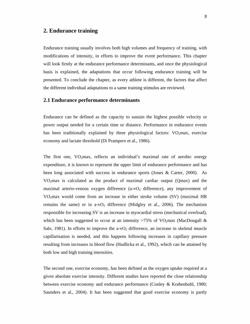
To further understand HRV, it might seem to be the oscillation between consecutive
instantaneous heart rates, but what it is really measuring is the variation of the time
between consecutive beats, as it is usually derived from the RR-interval (RRI)
recordings due to the facility of recognising them, as shown in figure 3 (a-b) (Aubert et
al., 2003). In order to interpret the results from these recordings, different methods have

19
been proposed to evaluate the variability of RR intervals, the most popular and widely
used are time-domain and frequency-domain methods (TaskForce, 1996).
Time-domain methods are the simplest to perform, as they are easily to obtain with
simple statistical methods that could be done on a simple excel spreadsheet (Buchheit,
2014). However, it was said that their main limitation was the discrimination of the
activity of the different autonomic branches (Aubert et al., 2003). The most frequently
used parameters are:
Standard deviation of the normal-to-normal interval (SDNN) over the recorded
time interval. These parameters represents the total variance of HR, but is
largely influenced on the length of the recording period, thus, when compared, it
should be done from recording with the same durations (TaskForce, 1996)
Square root of the mean squared differences of successive normal-to-normal
intervals (RMSSD). This parameter is the most commonly used, especially in
sport science research. It is known that RMSSD is an index of the
parasympathetic modulation, and is not very affected by breathing pattern, thus,
being highly recommended for field settings (Buchheit, 2014).
Frequency-domain methods were first introduced by Akselrod et al. (1981) to
quantitatively evaluate the beat-to-beat cardiovascular control. Power spectral density
(PSD) analyses give information of how power distributes as a function of frequency,
and the computation of power in defined frequency regions could give information
about the contribution of the different ANS branches (Aubert et al., 2003).
The most commonly used spectral analysis is Fast Fourier Transform (FFT) due to the
simplicity of the algorithms used, and the spectral components calculated from this
method are (figure 3c):
Very low frequency (VLF) represents the frequency band < 0.04 Hz, and is
though to relate, among other factors, to thermoregulation and kidney
functioning.
Low frequency (LF) represents the frequency range of 0.04 – 0.15 Hz, which
represents oscillations linked to regulation of blood pressure and vasomotor
tone, and is considered to be regulated by both parasympathetic and sympathetic
outflows.
20
High frequency (HF) represents the frequency range of 0.15 – 0.4 Hz, which
reflects the effects of respiration on HR (also referred to as respiratory sinus
arrhythmia), is considered to represent the parasympathetic efferent activity.
Total Power (TP), which represents all the frequency bands below 0.4 Hz, and it
is considered as an index of total variability.
Figure 3. Analysis of the heart rate variability obtained from a resting recording. (a) graphical
representation of consecutive RR intervals; (b) frequency domain analysis graph; (c) time
domain analysis results; (d) results from a 24h recording. Obtained from Aubert et al., (2003).
It is generally accepted that time-domain indices mainly reflects respiratory sinus
arrhythmia, which is mediated by parasympathetic vagal outflow, thus, being
considered as vagal tone indices (TaskForce, 1996; Goldstein et al, 2011). Regarding
the frequency-domain indices, HF band has been shown to decrease, together with LF
and TP, after a complete vagal blockade (Martinmäki et al., 2006), being considered as
a marker of vagal tone (TaskForce, 1996). On the other hand, the interpretation of LF

21
band remains controversial (Reyes del Paso et al., 2013), as it has been traditionally
proposed to reflect sympathetic tone, or to be affected by both parasympathetic and
sympathetic branches. However, growing evidence show that LF is not correlated with
sympathetic outflow (Baumert et al., 2009), and that it does not increase, but rather
decreases, when cardiac beta-adrenergic stimulation (which increases HR and plasma
norepinephrine levels) is applied (Ahmed et al., 1994). Finally, it is currently suggested
that LF band reflects the modulation of cardiac autonomic outflows by baroreflexes
(Goldstein et al., 2011).
3.2 HRV as a tool to monitor endurance training adaptations
Due to the increasing interest in monitoring parameters linked to performance and
fatigue, in efforts to improve the load-recovery balance, HRV has been proposed as a
promising tool for adjusting training loads and preventing the athlete to fall into an
overreaching state (Meeusen et al., 2013).
The 1990’s decade represents the start point of HRV use in sports, and from there on,
there has been a big increase in HRV studies reporting cross-sectional and longitudinal
data from athletes of different levels. Over these years, different and contradictory
findings have been reported, showing some studies that these measures are sensitive to
fitness improvements, fatigue, overload and detraining, while others have not (Plews et
al., 2013a).
Measures of autonomic activity, measured at baseline, have been suggested to predict
endurance performance (Flatt & Esco, 2014; Vesterinen et al., 2014a), and training
responses in untrained or relatively trained subjects (Hautala et al., 2003; Buchheit et
al., 2010). Studies looking at the time-course of changes in the ANS status and
endurance performance are various (Pichot 2002; Plews et al., 2013b) suggesting that
positive and negative changes in endurance performance are linked to changes in HRV.
However, due to high day-to-day variation in HR-derived indices, it is suggested to
assess training adaptations over changes on weekly averages, and not from single data
points (Plews et al., 2012; Buchheit, 2014). Furthermore, resting HRV (measured as

22
nocturnal TP) has been recently proposed as a marker of trainability of high-intensity
training for endurance runners (Vesterinen et al., 2014).
As HRV represents the vagal tone, it is normally higher during resting states. Night
recordings have been suggested as more reliable measurements due to the independence
of the measurement on environmental factors, and may better discriminate from real
changes in the autonomic nervous system (Pichot et al., 2000). Despite being night
recordings a more controlled situation, Hynynen et al. (2006) found that HRV after
awakening is more sensitive to chronic athletic stress suggesting that these
measurements could provide important additional information of the ANS status.
Moreover, the measure that could be collected more frequently (morning measure) is
likely to be the most powerful one, as it can decrease the noise of measurement when
performed daily (Buchheit, 2014).
3.3 Methodological factors affecting HRV
Billman (2011) suggested recently on his work on the HRV history that: “The internal
and external consistency of the methods used have received comparatively less research
interest than the understanding of the autonomic, cardiac and circulatory which creates
those methods”. Similar to this, it has been argued that the contradictory findings
published to date in the sports science field may be related to methodological
inconsistencies and/or partial misinterpretation of the data rather than to limitations of
HRV (Buchheit, 2014).
Studies looking at HRV reliability are usually done by means of the test-retest method,
with the retest usually done after several days or weeks (Cipryan et al., 2013). It is
known that the activity of the ANS system is very sensitive to different external and
internal factors, thus, the inter-day variability can consequently be significant. These
factors may contribute to the inconsistent results found in HRV studies (Cipryan et al.,
2013; Buchheit, 2014).
Reliability studies have also shown a higher CV and associated random error, especially
for the frequency-domain parameters (Pinna et al., 2007; Al Haddad et al., 2011),

23
suggesting that the time-domain methods may be more suitable for reducing the noise of
successive measurements. Plews et al. (2012) suggested that single-day data was not
enough to conclude whether an athlete is suffering from overreaching or overtraining,
due to the high day-to-day variability of the ANS and HRV, so he suggested to use a 7-
day rolling average in order to reduce the error and be able to obtain more accurate
information about the ANS status of an athlete. A time-domain parameter was used in
this study (RMSSD values), due to the reasons above mentioned. This new perspective
of the HRV monitoring (averaging consecutive days) aims to assess more accurately the
changes in the ANS status.
Additionally, the different methods of assessing the cardiac ANS adaptation to training
found in the literature are uneven: repeated measures of resting diurnal HRV (Buchheit
et al., 2010; Vesterinen et al., 2013), resting nocturnal HRV (Nummela et al., 2009),
exercise HR (Scharhag-Rosenberger et al., 2009), post-exercise HRR (Lamberts et al.,
2009), and post-exercise HRV (Buchheit et al., 2008). These variables are thought to
have a different time course of adaptation over a training intervention, and it remains to
be investigated whether they would provide an equivalent level of information on the
training adaptations (Buchheit et al., 2010).
In the following figure (4), an example of the different measurements that can be carried
out throughout the day are shown. HRV can be measured in many different situations,
however, not only the different measurements possible, but also the duration (1 min, 5
min, 4 h) and the position of the measurement (supine, standing, or seated), are part of
the different methodological variations that may affect to the controversial findings in
the literature (Esco & Flatt, 2014; Plews et al., 2012; Hynynen et al., 2006).

24
Figure 4. Example of different HR-derived measurements obtained during the day time: resting
heart rate variability (HRV), exercise heart rate (HR), heart rate recovery (HRR), and post-
exercise HRV (Buchheit, 2014).
Furthermore, another of the methodological variations when comparing between
different studies is the methods used to calculate HRV, using either time-domain or
frequency-domain parameters. In the latter years, the use of time-domain parameters,
such as RMSSD, has increased due to its simplicity, and due to its lower sensitivity to
free paced breathing, and makes it an ideal parameter to measure in day-to-day
monitoring under spontaneous breathing in athletes (Buchheit, 2014).
25
4 Central nervous system
The central nervous system (CNS) is a complex system containing more than 100
billion neurons that constantly receive information. One of the most important functions
of the CNS is to process incoming information in a way that appropriate mental and
motor responses will occur (more than 99% of all the sensory information is considered
by the brain as irrelevant). When important sensory information arrives, it is
immediately channelled into proper integrative and motor regions of the brain to cause
desired responses, this is the integrative function of the CNS (Guyton & Hall, 2006; p.
555).
Traditionally, the role of the CNS on endurance performance – understood as fatigue
appearance - has been controversial. Early works from Mosso (1915) proposed that
fatigue was from both central origin (nervous) and from peripheral origin (muscle).
Later on, the group led by Hill (1923) argued that endurance performance was limited
peripherally by an accumulation of metabolites at muscle level because of the limiting
capacity of the heart to supply oxygen to muscles, thus causing muscle anaerobiosis in
the skeletal muscle. In the latter years, a growing body of evidence has supported the
important role that the CNS plays in fatigue appearance, and thus, endurance
performance. One of the theories, the so called “central governor” model, was first
proposed by Noakes (2011), and suggested that the CNS regulates exercise specifically
to insure that each exercise bout ends whilst homeostasis is retained in all bodily
systems, and that the limiting factor of endurance performance resides in the brain.
The most important role of the CNS is to control the various bodily functions by
controlling the contraction of appropriate muscles throughout the body, the contraction
of the smooth muscle in the internal organs, and the secretion of active chemical
substances by exocrine and endocrine glands in the body (Guyton & Hall, 2006; p.
556). Operating in parallel to this axis is the ANS (as shown before with the figure 5),
which has been explained in the previous chapter.
Three major levels of the central nervous system have specific functional
characteristics: the spinal cord level, the subcortical level (lower brain area), and the

26
cortical level (higher brain area). For instance, the spinal cord level can cause walking
movements, and different reflexes (i.e., control of blood vessels). The lower brain area
controls most of the subconscious activities of the body (i.e., equilibrium, arterial
pressure, anger, etc). For the higher brain area, it is considered a large memory
storehouse which functions always in association with the lower brain centres to
precisely determine the operations to be done (Guyton & Hall, 2006; p. 558).
This review will focus on the role of the cerebral cortex (the outer cortical layer of the
brain), which is made up of neuron’s bodies, each of them receiving thousands of
synaptic inputs, giving rise to a complex processing capability (Guyton & Hall, 2006; p.
685). The cerebral cortex consists of two hemispheres, such as right and left
hemispheres. Each hemisphere can be divided into the following most prominent lobes:
frontal, parietal, occipital and temporal. These lobes are responsible for a variety of
bodily functions (as seen in figure 5):
Frontal lobe is involved with personality, emotions, problem solving, motor
development, reasoning, planning, parts of speech and movement.
Parietal lobe is responsible for sensation (e.g. pain, touch), sensory
comprehension, recognition, perception of stimuli, orientation and movement.
Occipital lobe is responsible for visual processing.
Temporal lobe is involved in dealing with the recognition of auditory stimuli,
speech, perception and memory.
Figure 5. Functional areas of the human cerebral cortex (Guyton & Hall, 2006; p.715)

27
The CNS is known to be an extremely complex system that is far away from being
completely understood. Recent research in the sports field has shown that a decline on
motor cortex activity plays a role in endurance exercise termination (Robertson &
Marino, 2015), supporting the previously mentioned line that suggests that the brain
regulates exercise performance. In addition, the increasing interest of identifying the
readiness of an athlete to train or to perform optimally, makes attractive to every sport
scientist the integration of a parameter that would provide us with information about the
status of the CNS. Despite the increasing amount of research trying to understand the
influence of the CNS on exercise performance, empirical data available for evaluating
the readiness of the CNS to perform optimally is lacking.
4.1 Neurophysiological basis of EEG and DC recordings
The electroencephalography (EEG) method was first developed by the German
psychiatrist Hans Berger, and was considered as an historical breakthrough as it
provided a new neurologic and psychiatric tool at that time (Tudor et al., 2004). The
EEG records electrical activity from the cerebral cortex, this electrical activity is
measured in microvolts (µV) and it must be amplified by a factor of 106 in order to be
displayed. Most of what it is recorded is known to be originated from neurons, but there
are other possible sources including action potentials, post-synaptic potentials, and
chronic neuronal depolarization (Rowan & Tolunsky, 2003; p. 1).
Complex neuronal electrical activity generates EEG signals that translate into random
and changing EEG waves. The physiological understanding of the underlying
mechanisms of EEG rhythmicity, although not completely understood, is mediated
through two main processes. Firstly, the interaction between cortex and thalamus, due to
the activity of the thalamic pacemaker cells, lead to rhythmic cortical activation.
Secondly, is based on the functional properties of large neuronal networks in the cortex
that have an intrinsic capacity for rhythmicity. The combination of both results in the
creation of recognizable EEG patterns, varying in different areas of cortex, that allows
to make sense of the complexity of brain waves (Rowan & Tolunsky, 2003; p. 2).

28
Traditionally, frequencies higher than 4 Hz were considered as valuable, and a major
obstacle was encountered in attempts to faithfully record slow events (also called DC-
potentials). Electrode drifts that produced artefactual slow signals tended to saturate the
amplifier’s dynamic range, and they also pushed the polygraph recorder pens out of
scale. To discard these problems, the EEG amplifiers became furnished with an in-built
high-pass filter, thus, all kinds of slow signals, whether physiological or artefactual,
were eliminated (Vanhatalo et al., 2004).
While it is evident that fast EEG activity has a neuronal origin, slow EEG signals may
arise from a variety of sources, including both neuronal and non-neuronal generators.
The work of Birbaumer et al. (1990) suggests that the slow potentials represent a
measure of excitability of cortical neuronal networks. Based on his findings, the surface
potential is affected by the level of polarisation or depolarisation of the dendritic tree in
vast networks of pyramidal cells, thus, indicating the level of excitability of the
underlying cortical tissue.
The introduction of the DC-potential in the sport field can be attributed to the work of
Ilyukhina (1982), where the findings are summarized upon the results of the
investigation done on 2900 healthy athletes. The purpose of this work was to recognise
the mechanisms of regulation of functional states of the organism as a whole, searching
for an integral parameter that would accurately reflect the adaptability of the organism
during changing external environmental conditions. From these experimental studies, it
was suggested that the time course of the very slow processes of secretory organs and
muscles, depended on changes in the state of the CNS, and that was accompanied by
reorganisation of very slow activity of the brain and spinal cord. From these findings, he
concluded that it was demonstrated the universality of very slow processes as a
physiological parameter of the state of the organs and tissues.
From a practical point of view, different patterns of decreasing or increasing the
potential following a loading test would demonstrate an optimal activation of the
nervous regulation (i.e., 25% increase of the initial values 3 min after the loading).
Furthermore, a decrease of more than 50% would mean an unfavourable sign of
exhaustion or disturbance of the nervous system. To conclude, Ilyuhkina et al. (1982)
suggested that the time-course of the DC-potential can be used to assess changes in the

29
functional state of the athletes, and that this would enable the training process and
recovery to be optimised depending on the daily state of this parameter. It remains to be
elucidated whether these findings can be practically applied and be meaningful in
athletes.
To the best of our knowledge, there are not many studies linking EEG patterns and
performance. Del Percio et al. (2009), together with Babiloni et al. (2010), have
attempted to test the hypothesis that ‘neural efficiency’ (measured as power decrease in
the alpha rythms, 8-12 Hz) is optimised in elite athletes. Their studies were limited to
cross-sectional data and to explosive sports like karate, fencing or rifle shooting, where
decisions are made in a relatively short period of time. Their findings showed that elite
athletes exhibited lower readiness potential (RP) and mean potential (MP) amplitude,
meaning a reduced cortical information processing. They suggested that these rhythms
reflected the functional mode of the thalamo-cortical and cortico-cortical loop that
facilitates/inhibits the integration of both sensorimotor and cognitive information into
the brain, and that these low- and high-frequency alpha rhythms were associated with
global brain arousal and the subject’s attentive readiness. Whether these alpha rhythms
may change longitudinally with training, and if these changes would provide a window
of trainability/readiness remains to be explored.
4.2 Methodological factors affecting EEG and DC-potential
measurements
Different factors may influence the recordings of the DC-potential, similarly to those
found in EEG recordings, thus, the methodological factors that affect both the EEG and
the DC-potential recordings will be presented. To start, the measurements of voltage,
obtained from the scalp, always refers to a relative difference in potential energy
between two points being monitored. The potential measured is dependent upon the
activity present at the ground measure, and the location of a reference electrode should
be ideally silent in electrical activity. This relativity of bioelectric recording must be
taken into consideration when interpreting EEG data and when forming subsequent
conclusions. Ideally, a ground or distant reference point would be a point in space
which is electrically stable and which would contribute no fluctuations of electrical

30
activity to measurement. However, there is no point on the body that is electrically
stable, but using the referential electrode placed distanced from the scalp would ideally
not reflect any brain wave activity (Fehmi & Collura, 2007).
Secondly, the placement of the electrodes on the scalp is of great importance. This was
first standardized in the 1950’s in order to provide reproducible research over different
laboratories, and this was called the 10-20 international placement system (Rowan &
Tolunsky, 2003; p. 3). A lateral image of the electrode placement 10-20 international
system can be seen in the figure 6. It has been shown that measuring the potential
fluctuations when recorded not only from the cortical surface but also from different
cortical layers, it can be shown that potential fluctuations in the latter recording may
differ considerably from those at the surface (Speckmann et al., 2004). This can be also
seen when recording from different electrode placements, as the intensity of the
potential may be from a difference source.
Figure 6. The international 10-20 electrode placement system for EEG applications. (Rowan &
Tolunsky, 2003; p. 5).
Studies looking at electroencephalography recordings include different frequency bands
ranges. The most common one used in the literature are the following (Rowan &
Tolunsky, 2003; pp. 25-28):

31
Delta activity (< 4Hz band) is not present in the normal adult, and when present,
it implies some kind of cerebral dysfunction (i.e., vascular disease).
Theta activity (4-7 Hz band) is usually present in the waking adult, and it should
by symmetrically distributed to represent normal function, otherwise it would
represent an underlying structural injury, but usually less malignant than what is
found in the Delta band.
Alpha activity (8-13 Hz band) is the principal activity of the normal adult, being
at its best when the subject is in a relaxed state with closed eyes, and a certain
degree of symmetry between hemispheres is needed for a normal functioning of
the brain.
Beta activity (> 14 Hz band) is always present, and an absence of it may
represent an abnormality, and a certain degree of symmetry is expected if there
is a correct functioning of the brain.
The frequency band used in this study is further reduced to a 0-0.5 Hz band, and
it is called DC-potential or ultra/infra slow activity (Vanhatalo et al., 2004).
To conclude this chapter, it is necessary to highlight the need of standardizing the
protocol when using EEG data in research, especially because the abovementioned
factors will influence the results obtained. From a practical point of view, to be able to
use the information obtained from the scalp, in the field, it is first needed to be easy to
use, and to be consistent with the results obtained in similar controlled conditions.
These requirements are necessary to be able to differ between a real change in the state
of the CNS with confounding factors (i.e., noise of the measurement).
32
5. Aim of the study
The discrepancies found in the literature regarding HRV have been mainly attributed to
methodological differences between experiments (Buccheit et al., 2014). To the best of
our knowledge, there is limited research regarding these methodological differences,
and one of the important issues is the reliability of HR-derived indices comparing
home-based measurements versus lab-based measurements done on the same day (±
2h). Furthermore, the different methods used in the literature (i.e., nocturnal
measurements) to assess HR-derived indices have not been compared to see whether
they differ or not when monitored on the same day.
On the other hand, new methods that could potentially monitor fatigue are needed in
order to make better decisions upon modifying an athlete’s training. To the best of our
knowledge, there is no empirical data looking into DC-Potential changes from home to
lab measurements done on the same morning. Furthermore, changes in DC-potential
following an increase in training intensity have not been reported. To conclude, as both
HR and HRV (i.e., RMSSD) have been suggested to be related with changes in
endurance performance, it is important to determine which index would better predict
the changes in performance seen over the 8week intervention period.
The aims of the study were:
1. To compare the HR-derived indices and DC-potential obtained in the morning at
home with those obtained in the lab in the same morning.
2. To compare HR-derived indices from morning and nocturnal recordings
obtained on the same day.
3. To determine if DC-potential is changed following a high-intensity training
period when compared to changes over a low-intensity training period.
4. To determine if HR or RMSSD could predict the changes in endurance
performance occurred over the 8week training intervention.

33
6. Methods
6.1 Study design
The study was designed to compare different monitoring variables throughout the 15
weeks period (Figure 7). Subjects performed endurance tests and basal testing at three
time points (PRE, MID and POST). Every subject was assigned with a device
(Omegawave Oy; Espoo, Finland) that was automatically synchronised with the lab
computer and daily checked by a researcher. Subjects were instructed after the PRE
measurements how to self-assess HR-derived indices and DC-Potential at home, and
were requested to do it daily throughout the intervention period. Moreover, a Garmin
Forerunner 610 was assigned and used by every subject during all their training
sessions, and to were requested to wear it during at least 4 nights a week. Training and
nocturnal data was sent to a project researcher once a week, and later analysed.
WEEK0
WEEK5
WEEK14 PERIODIZED
TRAINING
(50% LIT + 50% HIT)
INDIVIDUALISED TRAINING
BASED ON HRV
4 WEEKS 8 WEEKS
PRE MID POST
Figure 7. Experimental design of the study. Low-intensity training (LIT); High-intensity training (HIT).

34
6.2 Subjects
Twenty recreational runners were recruited, but only eighteen subjects performed all
testing and measurements (10 men, age 36.4 ± 6.1 yr; height 178.3 ± 5.2 cm; weight 77.8
± 6.2 kg; VO2max 55.7 ± 6.0 ml/kg/min; 8 women, age 34.1 ± 7.5 yr; height 166.8 ± 6.7
cm; weight 61.7 ± 7.5 kg; VO2max 47.1 ± 4.8 ml/kg/min). The inclusion criteria on
entering the study were: have a background of at least two years of endurance training,
age between 18-45 for men and 18-50 for women, body mass index (BMI) less than 30,
non-smoker, and a health status without any chronic diseases or prescribed medications.
Before the start of the project, all subjects underwent medical screening to ensure that
they presented a normal ECG pattern. After comprehensive oral and written
explanations of the study, all subjects gave their written informed consent. The Ethics
Committee of the University of Jyväskylä, in accordance with the Declaration of
Helsinki, approved this study.
6.3 Training intervention
The training intervention had a total duration of 12 weeks that was divided into two
parts. During both parts of the study, the subjects were allowed to perform once a week
a circuit training strength session and one training session of a different mode than
running (i.e., cycling).
i) The first part of the study consisted of a 4-week preparation period where subjects
followed a periodized training program with half of their weekly sessions done at low-
intensity and the other half was done at moderate- or high-intensity. In this first part of
the study, training was adjusted individually to maintain their usual frequency and
volume of training, however training intensity was changed. This period followed a
classical structure where three weeks of progressive training was followed by one week
of low-intensity training with reduced volume.
ii) The second part of the study consisted of an 8-week training period guided by
morning RMSSD values. Individual optimal area was established as the smallest
worthwhile change (SWC) of RMSSD, based on the recordings obtained from the first
part of the study. If the subject 7-day rolling RMSSD went below or above this SWC
35
line, subjects were asked to rest or perform low-intensity training. On the other hand, if
the 7-day rolling RMSSD stayed within the SWC area, high-intensity training sessions
were scheduled.
6.4 Data collection and analysis
Maximal Incremental Treadmill Test. The incremental running test was done on a
motorized treadmill (Rodby RL3500E, Vänge, Sweden) with the inclination set at 0.5º.
Before the test, subjects were asked not to do any vigorous physical activity two days
before, and were allowed to warm up for 5 min at the corresponding first stage speed of
the running test. The test was started at a speed of 7 km/h for women, and 8 km/h for
men, and was further increased every 3 min by 1 km/h until volitional exhaustion. The
test was considered as maximal when: RER was higher than 1.05, reported maximal HR
was achieved, and/or VO2 consumption showed a plateau. VO2max value was taken
from the highest VO2 value over a 60 s period. Before each test session, the gas analyser
(Oxycon Mobile, Viasys Healthcare GmbH, Hoechberg, Germany) was calibrated, and
breath-by-breath data of ventilation and respiratory gases, as well as HR (Suunto T6,
Suunto Oy, Vantaa, Finland), were continuously monitored throughout the test.
3km Time Trial. Every subject ran a maximal 3000m time trial (TT) in a 200m indoor
running track (Jyväskylä, Finland). Timing was done by an experienced researcher, and
feedback was individually given after every lap. HR (Garmin Forerunner 610, Garmin
Ltd., UK) was recorded throughout the test and was used for analysis together with the
ending time.
Diurnal OMEGAWAVE measurements. Upon waking, subjects were asked to place two
electrodes (one in the hand palm and another one in the mid of the forehead, as
indicated by the manufacturer, as seen in the figure 8) in order to quantify the direct
current potential of the brain (Omegawave Oy; Espoo, Finland) from the scalp (at Fpz
area following international placement 10-20). The subjects were asked to stay in a
supine position, with eyes closed and in a quiet environment. The measurement length
was until the DC-potential stabilisation, and usually lasted 4 minutes. Together with
this, the subjects were asked to measure their RR intervals (Omegawave Oy; Espoo,

36
Finland) placing a heart rate belt over their chest. The RR data was recorded together
throughout 4 minutes and analysed with the Omegawave software. Because of software
limitations, artefact correction was not possible, thus, measurements with no more than
2 artefacts were taken into account. Breathing was not controlled and was free paced, as
research has shown that RMSSD remains consistent across different breathing patterns
(Esco & Flatt, 2014). The individual mobile device of every subject was synchronized
with a computer placed in the Physiology Lab (KIHU) and daily updates of their HRV
profile was done every morning. Furthermore, during the measurement weeks (PRE,
MID and POST), all lab tests were performed between 07.00 and 08.00 hours, with the
subjects lying down on a stretcher in a supine position. The room was kept at a
comfortable temperature, and before every measurement started, lights were turned off
after verifying that there was a complete silent situation.
Figure 8. Example of the placement of both electrodes: a) on the palm of the dominant hand,
and b) on the Fpz 10-20 international placement on the forehead.
Nocturnal HR-derived indices. The subjects were asked to measure nocturnal RR
intervals during at least four nights per week throughout the training study. A HR
monitor (Garmin Forerunner 610, Garmin Ltd., UK) was used to record RR intervals
with a sampling frequency of 1000 Hz. The recording started before going to bed and
was stopped upon waking in the morning. The first 30 min of recording was excluded
and the following continuous 4-hour period was accepted for the analysis if the imposed
37
cut-off of the erroneous RR intervals was lower than 33%. The acceptable RR interval
data was processed and analysed using the Firstbeat Sports heartbeat analysis software
(version 2.0.0.9, Firstbeat Technologies Ltd., Jyväskylä, Finland). RR interval
recordings were first scanned through an artefact detection filter of the Firstbeat PRO
software to exclude all falsely detected, missed and premature heart beats (Saalasti,
2003). Time-domain and Frequency-domain data was obtained from these recordings.
HIT week or LIT week. HIT week was considered when there was no more than one
low-intensity session and the rest of the sessions performed were high-intensity training.
A lower training load and lower time spent above VT1 was expected for the control
week (LIT) versus the HIT week. Seven day rolling DC-potential, HR and RMSSD,
both in absolute and relative changes, were analysed.
6.5 Statistical analysis
The data was analysed using SPSS 19 (SPSS Inc, Chicago, USA). All data are
presented as mean (SD). The distribution of each variable, as well as the difference
between tests, was visually inspected for normality distribution by Q-Q plots, and
further explored with the Shapiro-Wilk normality test.
To assess the reliability of measures of HR-derived indices different methods have been
proposed in the literature (Atkinson & Nevill, 1998). In this study, a specifically
designed spreadsheet was used (Hopkins, 2000), which provides reliability statistics for
consecutive pairs of trials for each individual when there are at least two trials. HRV
data was log transformed in order to assure a better distribution of the data. The
following indices were chosen to assess reliability: i) Pearson’s product-moment
correlation analysis; ii) typical error of measurement with 95% confident intervals; iii)
Intraclass correlation coefficient (ICC) with 95% confidence intervals; iv) Coefficient
of Variation (CV); and v) Limits of Agreement (LoA) with the bias between pair of
measurements ± 1.96 SD.
To assess the relationship between morning measures (upon awaking) and lab
measurements assessed in the same morning, a total of 33 cases from 18 subjects were
38
obtained. To establish the agreement between nocturnal and morning measurements,
data from 18 subjects all over the 12 week period was obtained, and a total of 494 cases
were accepted for analysis.
To assess the sensitivity of DC-Potential to high-intensity training (HIT) periods, all
training sessions during the last 8 week period were visually inspected for each subject,
to obtain a control week were training load is low and done only in a low-intensity
(LIT) manner, while a HIT period was established as a week were all except one of the
trainings were done with high-intensity. Training load data, calculated from a modified
TRIMP version (Lucia et al., 1999) was calculated for each session and week.
Furthermore, the time above the VT2 was calculated to better show the difference
between training periods. Due to the large CV of the daily DC-potential, a 7-day rolling
average was used as it has been proposed for HRV measurements (Plews et al., 2012),
and the difference between the first (1st) and last (7th) day of each period was compared
in absolute and relative values to the control week using a paired student’s t-test, with
significance established at p<0.05. From the 18 subjects, we were only able to establish
a control week and a HIT week for 13 subjects. From these subjects, a total of 20 cases
were taken into analysis.
To evaluate the training adaptation, HR and RMSSD, both at a single point and as a
weekly average, were analysed. Prior the calculations, uniformity of the variables were
examined. A total of 14 subjects were taken into analysis. Pearson’s product-moment
correlation analysis was used to determine the association between relative changes in
endurance tests and the HR-derived indices. The following criteria were adopted to
interpret the magnitude of the correlation (r) between test measures: <0.1, trivial; 0.1-
0.3, small; 0.3-0.5, moderate; 0.5-0.7, large; 0.7-0.9, very large; and 0.9-1.0, almost
perfect.

39
‐2
‐1,5
‐1
‐0,5
0
0,5
1
1,5
2 2,5 3 3,5 4 4,5 5 5,5
Hom
e‐LabMeasurement
(LnRMSSD)
MeanLnRMSSD
7. Results
Agreement between Home and Lab HR-indices
A summary of the different reliability indices used can be found in table 1. There was a
significant difference between home and lab for all the indices except for Ln LF and Ln
HF (P > 0.05). The moment Pearson correlation showed that HR had a large correlation
(r = .809), while Ln HF (r = .575) and Ln RMSSD (r = .647) had a moderate agreement,
with the rest of the measurements having a low agreement. When examining closely the
data, large individual variations were found. In HR, 17 cases fall within ± 5 bpm, while
8 cases had differences larger than 10 bpm between the home and lab measurements.
Figure 9 shows the difference within each pair of measurements for the Ln RMSSD.
Figure 9. Bland Altman plot with the within-subject differences between the measurement
done at home and in the lab in Ln RMSSD.

40
Table 1. Agreement of HRV parameters between two tests done the same morning at home and in the lab.
Test Reliability
Cases Home(i) Lab(ii)Pearson
Correlation
TypicalError
[95%CI]
ICC
[95%CI]CV(%)
LoA
Bias[±1.96
SD]
HR 33 52.6(7.9) 56.5(11.6)* .809* 4.93[4.0;6.5] .754[.555;.872] 8.9 3.9[±13.7]
LnRMSSD 33 4.28(0.63) 4.01(0.65)* .647* 0.38[0.31;0.51] .647[.390;.810] 9.8 ‐.27[±1.06]
LnLF 32 6.81(1.05) 6.54(1.03) .427* 0.79[0.63;1.05] .427[.092;.675] 12.7 ‐.27[±2.18]
LnHF 32 6.67(1.35) 6.18(1.34) .575* 0.88[0.70;1.17] .575[.283;.769] 15.1 ‐.49[±2.43]
LnTP 32 7.69(0.99) 7.31(0.97)* .492* 0.70[0.56;0.93] .492[.172;.717] 9.8 ‐.38[±1.94]
DC‐Potential 30 15.94(12.6) 18.15(11.1)* .293 9.98[7.95;13.42] .291[‐.077;.589] 81.6 4.03[±19.88]
ICC = Intraclass Correlation Coefficient; CV = Coefficient of Variation; LoA = Limits of Agreement; Bias = mean difference between criterion and repeated
measure; [95% CI] = 95% confidence intervals for typical error and ICC. Significance (*) is set at P < 0.05. HR = Heart Rate; Ln RMSSD = Natural logarithm
of the square root of the mean squared differences of successive normal-to-normal intervals; Ln LF = Natural logarithm of Low Frequency power; Ln HF =
Natural logarithm of High Frequency power; Ln TP = Natural logarithm of Total Power; DC-Potential = Direct current potential of the brain.

41
Agreement between Nocturnal and morning HR-indices
A summary of the different reliability indices used can be found in table 2. There was a
significant difference between nocturnal and morning measurements for every variable
(P < 0.05). A large correlation was found in the variables HR (r = 0.692), Ln RMSSD (r
= 0.641) and Ln TP (r = 0.532), while a moderate correlation was found in Ln HF (r =
0.460). Despite the acceptable agreement in Ln RMSSD and HR, the limits of
agreement plot showed large within-subject differences between measurements (figure
10).
Figure 10. Bland-Altman plot of Morning and Nocturnal Ln RMSSD.

42
Table 2. Agreement of HRV parameters during two tests done at night and in the following morning.
Test Reliability
Cases Nocturnal Morning
Pearson
CorrelationTypicalerror
[95%CI]
ICC
[95%CI]CV(%)
LoA
Bias[±1.96
SD]
HR(bpm) 494 53.8(6.6) 54.2(7.8)* .692* 4.1[3.85;4.36] .683[.633;.728] 7.4 0.4[±11.3]
LnRMSSD(lnms) 494 4.06(0.50) 4.13(0.65)* .641* 0.36[.34;.38] .619[.562;.671] 9.1 .07[±0.99]
LnHF(lnms2) 494 7.94(0.67) 6.33(1.34)* .460* 0.84[.79;.90] .368[.289;.442] 22.2 ‐1.61[±2.33]
LnTP(lnms2) 494 8.56(0.75) 7.42(0.95)* .532* 0.59[.56‐.63] .518[.450;.580] 13 ‐1.14[±1.64]
ICC = Intraclass Correlation Coefficient; CV = Coefficient of Variation; LoA = Limits of Agreement; Bias = mean difference between criterion and repeated
measure; [95% CI] = 95% confidence intervals for typical error and ICC. Significance (*) is set at P < 0.05. HR = Heart Rate; Ln RMSSD = Natural logarithm
of the square root of the mean squared differences of successive normal-to-normal intervals; Ln HF = Natural logarithm of High Frequency power; Ln TP =
Natural logarithm of Total Power;

43
Sensitivity of DC-Potential to High-Intensity training periods
There was a significant difference (P < 0.05) between training load in the control week
(225 ± 100 AU) and the HIT week (333 ± 108 AU). In addition, there was significant
difference between the time spent above the VT2 in the control week (6 ± 8 min) and
the HIT week (135 ± 56 min). There were no significant difference of the relative
changes from day 1 to day 7, in the 7day rolling RMSSD, the 7day rolling HR, and the
7day rolling DC-potential indices, between the control and the HIT week (P > 0.05).
Furthermore, there were no significant differences between the absolute changes from
the day 1 to the day 7 in the abovementioned variables, between the control week and
the HIT week (P > 0.05). In the figure 11, an example can be seen of the differences
between a control week and a HIT week in one of the cases.
Figure 11. A graphical example comparing a control week and a high-intensity week of one
subject during the 8-week period. Dark grey bars represent HIT sessions, while light grey bars
represent LIT sessions.
0,00
5,00
10,00
15,00
20,00
0
20
40
60
80
100
Mon Tues Wed Thurs Frid Sat Sun
DC‐Potential(mV)
TrainingLoad(AU)
ControlWeek
0,00
5,00
10,00
15,00
20,00
0
20
40
60
80
100
Mon Tues Wed Thurs Frid Sat Sun
DC‐Potential(mV)
TrainingLoad(AU)
HITWeek
44
Prediction of endurance performance changes with HR-derived indices
No relationships were found between changes in morning HR (single data point) from
MID to POST and relative changes in Vmax speed (r = 0.094), VO2max (r = -0.167),
and speed in 3km TT (r = 0.072). Positive correlations were found between weekly HR
average relative changes from MID to POST and relative changes in Vmax speed (r = -
0.732; P < 0.01) and 3km TT (r = -0.636; P < 0.05) (Figure 12), and a tendency was
found with VO2max (r = -0.53; P = 0.051). Positive correlation was found between
changes in RMSSD (single data point) from MID to POST and relative changes in
VO2max (r = 0.650; P < 0.05), and no correlations were found with Vmax (r = -0.132),
and with 3km TT (r = 0.055). No correlations were found between relative changes in
weekly RMSSD average from MID to POST and relative changes in Vmax speed (r =
0.328), VO2max (r = 0.187), and speed in 3km TT (r = 0.444).
Figure 12. Relative changes from MID to POST measurements (8 weeks) in weekly HR and relative
changes in: i) speed at Vmax; ii) speed at 3km TT.

45
8. Discussion
To the best of our knowledge this is the first study to examine: 1) the agreement
between HR-derived indices obtained at home and in the lab in the same morning; 2)
the agreement between HR-derived indices obtained during nocturnal and morning
recording; 3) to examine the effects of high intensity endurance training on DC-
potential; 4) and to determine the relationship between changes in HR-derived indices
and changes in endurance performance.
The main findings of the study were: i) the agreement between HRV measures in the
same morning (home vs lab) showed acceptable agreement for HR, and questionable for
RMSSD, and Ln HF values; ii) the nocturnal and morning measurements showed poor
and questionable agreement for most of the indices, but HR and RMSSD seemed to be
the ones that have larger agreement; iii) DC-potential did not seem to be changed
following increases in training load, as seen during a HIT week period; iv) endurance
performance changes were correlated with weekly morning HR average changes, but
not with weekly RMSSD changes.
Agreement between Home and Lab HR-indices
The results of our study showed that there was an acceptable agreement between home
and lab measurements for HR (seen as ICC > .70), a questionable agreement for Ln
RMSSD and Ln HF (ICC .50 - .70), and variables such as Ln LF, Ln TP, and DC-
potential had a very poor agreement (ICC < .50). Conclusions from our findings cannot
be compared directly to HRV reliability studies (Al Haddad et al., 2011; Cipryan et al.,
2013) due to the inherent difference in the study design. These results show slightly
lower CV for time-domain variables (i.e., RMSSD), but higher difference with
frequency-domain parameters such as Ln HF and Ln LF when compared to the study of
Al Haddad et al. (2011). Moreover, for frequency-domain methods, results show larger
typical error and ICC when compared to the inter-day reliability (Cipryan et al., 2013).
This is the first study to address the agreement between successive measures of DC-
potential of the brain, done in different environments (home and lab) on the same day
(within 2h). Our results showed that the agreement is very poor (CV = 81.6%; ICC =

46
0.291). The origin of this low agreement between measurements may come from
different sources. First of all, the associated noise of the measurement is a factor that
has to be taken into account when using successive measurement. On the other hand,
this low agreement may reflect a different state of the CNS, as the second measurement
did not represent a completed rested state, as it was the first measurement. A different
state of the CNS may be expected after 1-2h after awakening, and this might be
reflected in the large differences between both measurements. However, these changes
were in some cases larger than what Ilyukhina et al. (1982) reported to be a change from
an optimal state to an exhaustion state (change in 50% of the initial value), making
difficult to conclude that this change was due to a change in the state of the CNS.
One of the limitations of the study is the standardization of the transport used (i.e.,
cycling) when subjects moved towards the lab. The influence that cycling has on a
subject’s subsequent measurement might have had an effect in some of the subjects, as
some subjects had very large differences between measurements (up to 18 bpm).
Furthermore, the influence of being in a laboratory should not be undervalued, as for
some subjects this first measurement done at the lab might have caused some excitation
or stress. In our study breathing pace was not controlled, and it is known that breathing
has an influence in the results, especially in frequency-domain methods (Buchheit,
2014). It is also possible that a difference the breathing, together with possible voluntary
or involuntary actions (like moving, swallowing, sneezing, coughing, or yawning) done
during the home measurement, would have influenced the lower agreement found in
HR-derived and DC-potential indices.
Agreement between Nocturnal and morning HR-indices
Our findings show that the agreement between morning and nocturnal HR-derived
indices range from poor (for the frequency-domain indices, Ln HF and Ln TP) to
questionable (for the time-domain variables, HR and Ln RMSSD). The nocturnal
recordings have been extensively used in HRV research studies (Nummela et al., 2009;
Hynynen et al., 2006; 2010; Pichot et al., 2000; 2002), due to the suggested less
sensitivity of the measurement to environmental factors, and because it may represent a
condition free of external disruptive events (Pichot et al., 2000). However, it has been
criticised because the 4h recording period analysed does not distinguish between sleep
stages, and thus, does not represent a standardised period, but rather a continuous

47
variation between sleep stages where different vagal or sympathetic dominance can be
found (Buchheit et al., 2004). Another method to measure nocturnal HRV has been
proposed by Buchheit et al. (2004). This method limits the measurement to a selected
slow wave sleep (SWS) period, which is the deepest stage of sleep, and is characterized
by a large vagal tone, and regular respiratory patterns. However, this method has not
been compared directly with consecutive morning measurement as done in this study,
neither it has been compared with the 4h method used in the present study. Thus,
whether the analysis of the SWS period is in agreement with the morning measurement
remains to be explored.
Recently, Buchheit (2014) suggested that the possible effects that different patterns of
sleep (time spent at different sleep stages) may have on these recordings have been
overlooked, and these different patterns may change over time independent from
training-related changes in ANS status, In our study, our results show that parameters
measured during night recording and morning recording might differ up to around 1 Ln
ms2 (figure 9), which may not be highly meaningful at low values (2-3 Ln ms2), but it
can be much more than meaningful at high values (4-5 Ln ms2).
The differences in the agreement between both methods might be partly explained by
the different timing of the measurement. The first one, the morning measurement, aims
to measure the HRV in a rested situation after awakening, where the levels of
circulating hormone and body temperature are low. On the other hand, the nocturnal
measurement, aims to measure the HRV of a subject over the night, and this period
includes different levels of hormonal secretion (i.e., growth hormone), and brain activity
throughout the different sleeping stages. Thus, it cannot be expected to obtain the same
result, but to give a partial agreement, and possibly to change similarly over time.
Future studies should look at the relationship between nocturnal HRV (with both
methods: SWS and 4h recording) and quality of sleep (measured as efficiency of sleep
and time at different stages), as it could be reflecting a different adaptation than the
morning measurement (i.e., efficiency of sleeping).
Sensitivity of DC-Potential to High-Intensity training periods
The results of our study show that neither of the measured variables (7day rolling
RMSSD, 7day rolling HR and 7day rolling DC-potential) change following high

48
intensity periods, when compared to low-intensity periods. HR-derived indices are
known to be affected by different factors. Vagal tone can be decreased the following
day after a training session with a large part of the training conducted above the second
ventilatory threshold (VT2), and can be increased following a low-intensity session
below the first ventilatory threshold (VT1) (Seiler et al., 2007). However, following a
longer high-intensity training period, the athlete can fall in an overreached state, where
evidence of up-regulation of vagal tone has been also reported (Le Meur et al., 2013).
Other factors different than training load (i.e., life stresses) have a large influence on
HR and HRV (Buchheit, 2014). These different findings make the interpretation of the
changes in HR and HRV even more difficult. Based on our findings, it can be suggested
that, due to the high day-to-day variation of HR and HRV, together with the different
changes expected following high-intensity or low-intensity periods, the interpretation of
training solely based on HR and HRV is not recommended. It can be argued that HR-
derived indices are more sensitive to chronic changes, as they have been extensively
proposed as a parameter to chronic fatigue (Buchheit, 2014).
Furthermore, for DC-potential measurement, the 7-day rolling average was chosen due
to its high CV even when done within 2h (CV = 81%). Whether high-intensity sessions
have an impact on the state of the CNS (measured as DC-potential) has not been studied
before. It is suggested that some of the factors that might have influenced the absence of
changes in 7-day DC-potential following HIT periods are the standardised conditions
that may be needed to get a reliable measure (Appendix I), and probably makes this tool
difficult to use in field settings. Acute changes were found (in single-point DC-
potential) following high-intensity training sessions, but of different direction and
magnitude. Thus, it remains to be elucidated whether individual patterns may help
optimize the usage of DC-potential as a monitoring tool.
Furthermore, future research should look at the influence of the placement currently
used for DC-potential measurement in the field, and to compare it to reference
placement (Cz position, Vertex) used in research (Ilyukhina et al., 1982), as it may not
reflect what the current research suggests. Based on our results, none of the
abovementioned parameters should be used independently, and decisions upon training
session changes should be done based on the individual variation of the ANS system,

49
and together with other parameters (i.e., subjective perception of effort) (Buchheit,
2014)
Prediction of endurance performance changes with HR-derived indices
The prediction of endurance performance based on HR-derived indices has been
extensively explored in the literature (Buchheit, 2014). However some of the studies
have been limited only to positive responders (Buchheit et al., 2010), or have not
compared it to VO2max changes (Plews et al., 2013b). Our findings suggest that weekly
morning HR average is the most sensitive parameter to evaluate changes in endurance
performance over time, and that it may be more sensitive than RMSSD in single data-
point (except for VO2max) and weekly average.
Single data-points of HR-derived indices for evaluating adaptations to endurance
training have received large critics in the last years (Plews et al., 2013b; Buchheit,
2014), arguing that it might hinder the bigger picture that could provide weekly average.
Our results show that weekly morning HR was more sensitive to changes in
performance than weekly RMSSD changes, as suggested in previous research (Plews et
al., 2013b). Resting HR might have changed due to a an increase in heart volume and
contractility, which would lead to a higher resting stroke volume, and this can be also
induced by an increase in blood volume (Aubert et al., 2003), which are common
adaptations following endurance training. Furthermore, the lack of relationship found
with resting RMSSD might be due to the lower influence of resting vagal tone changes
on endurance performance.
The associated day-to-day variation, the influence of environmental factors, and the
small error associated with the measurement device, might have had an effect on the
low relationship found with RMSSD in this study. Research in this field is limited, and
future studies should be looking at the relationship between changes in HR-derived
indices and changes in endurance performance in larger samples and in different trained
populations (from sedentary to well-trained athletes), in order to be able to make better
decision-based changes in training programs.
50
9. Conclusions
Based on our findings, it is recommended to use the different HRV measurements
independently from each other, as the agreement between them is most of the time
questionable or even poor. These indices might mirror different changes in the ANS
system at distinct time courses.
Furthermore, it is suggested that when introducing new monitoring tools in the training
programs, methodological consistency, together with standardization of the
measurement, should be regarded as the first step done before making training
adjustment based upon the measurement changes. Otherwise, it would not be possible to
differentiate between real changes and changes caused by confounding factors. To
conclude, it is highly recommended the use of a classical parameter, as it is morning
HR, especially when averaged weekly, in order to evaluate the adaptation course
following endurance training programs.
Practical Applications
From the practical point of view, morning measures upon waking at home represent the
most easy-to-use method to measure HRV (as it takes only 5 min), and it has been
suggested to be more sensitive to chronic fatigue changes (i.e., overtraining), when
compared to other methods (i.e., nocturnal recordings). Additionally, tracking weekly
changes in morning HR can be an effective, easy to implement, and a free way of
evaluating adaptations to endurance training over time.
51
10. References
Ahmed, M. W., Kadish, A. H., Parker, M. A., & Goldberger, J. J. (1994). Effect of
physiologic and pharmacologic adrenergic stimulation on heart rate variability.
Journal of the American College of Cardiology, 24(4), 1082-1090.
Akselrod, S., Gordon, D., Madwed, J. B., Snidman, N. C., Shannon, D. C., & Cohen, R.
J. (1985). Hemodynamic regulation: Investigation by spectral analysis. The
American Journal of Physiology, 249(4 Pt 2), H867-75.
Al Haddad, H., Laursen, P. B., Chollet, D., Ahmaidi, S., & Buchheit, M. (2011).
Reliability of resting and postexercise heart rate measures. International Journal of
Sports Medicine, 32(8), 598-605. doi:10.1055/s-0031-1275356 [doi]
Atkinson, G., & Nevill, A. M. (1998). Statistical methods for assessing measurement
error (reliability) in variables relevant to sports medicine. Sports Medicine, 26(4),
217-238.
Aubert, A. E., Seps, B., & Beckers, F. (2003). Heart rate variability in athletes. Sports
Medicine, 33(12), 889-919.
Babiloni, C., Marzano, N., Iacoboni, M., Infarinato, F., Aschieri, P., Buffo, P., Cibelli,
G., Soricelli, A., Eusebi, F., Del Percio, C. (2010). Resting state cortical rhythms in
athletes: A high-resolution EEG study. Brain Research Bulletin, 81(1), 149-156.
Banister, E. W., & Calvert, T. W. (1980). Planning for future performance: Implications
for long term training. Canadian Journal of Applied Sport Sciences.Journal
Canadien Des Sciences Appliquees Au Sport, 5(3), 170-176.
Baumert, M., Lambert, G. W., Dawood, T., Lambert, E. A., Esler, M. D., McGrane, M.,
Barton, D., Sanders, P., Nalivaiko, E. (2009). Short-term heart rate variability and
cardiac norepinephrine spillover in patients with depression and panic disorder.
American Journal of Physiology.Heart and Circulatory Physiology, 297(2), H674-
9. doi:10.1152/ajpheart.00236.2009 [doi]
Billman, G. E. (2011). Heart rate variability - a historical perspective. Frontiers in
Physiology, 2, 86. doi:10.3389/fphys.2011.00086 [doi]
Birbaumer, N., Elbert, T., Canavan, A. G., & Rockstroh, B. (1990). Slow potentials of
the cerebral cortex and behavior. Physiological Reviews, 70(1), 1-41.
Bishop, D. J., Granata, C., & Eynon, N. (2014). Can we optimise the exercise training
prescription to maximise improvements in mitochondria function and content?
Biochimica Et Biophysica Acta (BBA)-General Subjects, 1840(4), 1266-1275.

52
Blomqvist, C. G., & Saltin, B. (1983). Cardiovascular adaptations to physical training.
Annual Review of Physiology, 45(1), 169-189.
Bouchard, C., Leon, A. S., Rao, D. C., Skinner, J. S., Wilmore, J. H., & Gagnon, J.
(1995). The HERITAGE family study. aims, design, and measurement protocol.
Medicine and Science in Sports and Exercise, 27(5), 721-729.
Bouchard, C., Lesage, R., Lortie, G., Simoneau, J. A., Hamel, P., Boulay, M. R.,
Perusse, L., Theriault, G., Leblanc, C. (1986). Aerobic performance in brothers,
dizygotic and monozygotic twins. Medicine and Science in Sports and Exercise,
18(6), 639-646.
Bouchard, C., Sarzynski, M. A., Rice, T. K., Kraus, W. E., Church, T. S., Sung, Y. J.,
Rao, D. C., Rankinen, T. (2011). Genomic predictors of the maximal O(2) uptake
response to standardized exercise training programs. Journal of Applied Physiology
(Bethesda, Md.: 1985), 110(5), 1160-1170. doi:10.1152/japplphysiol.00973.2010
[doi]
Boullosa, D. A., Abreu, L., Varela-Sanz, A., & Mujika, I. (2013). Do olympic athletes
train as in the paleolithic era? Sports Medicine, 43(10), 909-917.
Buchheit, M. (2014). Monitoring training status with HR measures: Do all roads lead to
rome? Frontiers in Physiology, 5
Buchheit, M., Chivot, A., Parouty, J., Mercier, D., Al Haddad, H., Laursen, P., &
Ahmaidi, S. (2010). Monitoring endurance running performance using cardiac
parasympathetic function. European Journal of Applied Physiology, 108(6), 1153-
1167.
Buchheit, M., Millet, G., Parisy, A., Pourchez, S., Laursen, P., & Ahmaidi, S. (2008).
Supramaximal training and postexercise parasympathetic reactivation in
adolescents. Medicine Science in Sports Exercise, 40(2), 362.
Cipryan, L., & Litschmannova, M. (2013). Intra-day and inter-day reliability of heart
rate variability measurement. Journal of Sports Sciences, 31(2), 150-158.
Conley, D. L., & Krahenbuhl, G. S. (1980). Running economy and distance running
performance of highly trained athletes. Medicine and Science in Sports and
Exercise, 12(5), 357-360.
Consitt, L. A., Copeland, J. L., & Tremblay, M. S. (2002). Endogenous anabolic
hormone responses to endurance versus resistance exercise and training in women.
Sports Medicine, 32(1), 1-22.

53
Del Percio, C., Babiloni, C., Marzano, N., Iacoboni, M., Infarinato, F., Vecchio, F.,
Lizio, R., Aschieri, P., Fiore, A., Toràn, G. (2009). “Neural efficiency” of athletes’
brain for upright standing: A high-resolution EEG study. Brain Research Bulletin,
79(3), 193-200.
Dellaserra, C. L., Gao, Y., & Ransdell, L. (2014). Use of integrated technology in team
sports: A review of opportunities, challenges, and future directions for athletes.
Journal of Strength and Conditioning Research / National Strength & Conditioning
Association, 28(2), 556-573. doi:10.1519/JSC.0b013e3182a952fb [doi]
Di Prampero, P., Atchou, G., Brückner, J., & Moia, C. (1986). The energetics of
endurance running. European Journal of Applied Physiology and Occupational
Physiology, 55(3), 259-266.
Esco, M. R., & Flatt, A. A. (2014). Ultra-short-term heart rate variability indexes at rest
and post-exercise in athletes: Evaluating the agreement with accepted
recommendations. Journal of Sports Science & Medicine, 13(3), 535.
Farrell, P. A., Wilmore, J. H., Coyle, E. F., Billing, J. E., & Costill, D. L. (1993).
Plasma lactate accumulation and distance running performance. 1979. Medicine
and Science in Sports and Exercise, 25(10), 1091-7; discussion 1089-90.
Fehmi, L. G., & Collura, T. (2007). Effects of electrode placement upon EEG
biofeedback training: The monopolar-bipolar controversy. Journal of
Neurotherapy, 11(2), 45-63.
Fiskerstrand, Å., & Seiler, K. (2004). Training and performance characteristics among
norwegian international rowers 1970–2001. Scandinavian Journal of Medicine &
Science in Sports, 14(5), 303-310.
Flatt, A. A., & Esco, M. R. (2014). Endurance performance relates to resting heart rate
and its variability: A case study of a collegiate male cross-country athlete. J Aus
Strength Cond, 22, 39-45.
Goldstein, D. S., Bentho, O., Park, M., & Sharabi, Y. (2011). Low‐frequency power of
heart rate variability is not a measure of cardiac sympathetic tone but may be a
measure of modulation of cardiac autonomic outflows by baroreflexes.
Experimental Physiology, 96(12), 1255-1261.
Guyton, A.C. & Hall, J. E. (2006). Guyton and hall textbook of medical physiology
Elsevier Health Sciences.

54
Halson, S. L. (2014). Monitoring training load to understand fatigue in athletes. Sports
Medicine, 44(2), 139-147.
Heathers, J. A. (2014). Everything hertz: Methodological issues in short-term
frequency-domain HRV. Frontiers in Physiology, 5
Hickson, R. C., Hagberg, J. M., Ehsani, A. A., & Holloszy, J. O. (1981). Time course of
the adaptive responses of aerobic power and heart rate to training. Medicine and
Science in Sports and Exercise, 13(1), 17-20.
Hill, A., & Lupton, H. (1923). Muscular exercise, lactic acid, and the supply and
utilization of oxygen. Qjm, (62), 135-171.
Hopkins, W. (2000). Reliability from consecutive pairs of trials (excel spreadsheet). A
New View of Statistics,
Hudlicka, O., Brown, M., & Egginton, S. (1992). Angiogenesis in skeletal and cardiac
muscle. Physiological Reviews, 72(2), 369-417.
Hynynen, E., Uusitalo, A., Konttinen, N., & Rusko, H. (2006). Heart rate variability
during night sleep and after awakening in overtrained athletes. Medicine and
Science in Sports and Exercise, 38(2), 313.
Ilyukhina, V., Sychev, A., Shcherbakova, N., Baryshev, G., & Denisova, V. (1982). The
omega-potential: A quantitative parameter of the state of brain structures and of the
individual: II. possibilities and limitations of the use of the omega-potential for
rapid assessment of the state of the individual. Human Physiology,
Ilyukhina, V. A. (1982). The omega potential: A quantitative parameter of the state of
brain structures and organism. I. physiological significance of the omega potential
when recorded from deep structures and from the scalp. Human Physiology, 8(3),
221-226.
Jänig, W. (2006). Integrative action of the autonomic nervous system: Neurobiology of
homeostasis Cambridge University Press.
Jänig, W., & Häbler, H. (1999). Specificity in the organization of the autonomic
nervous system: A basis for precise neural regulation of homeostatic and protective
body functions. Progress in Brain Research, 122, 351-367.
Jones, A. M., & Carter, H. (2000). The effect of endurance training on parameters of
aerobic fitness. Sports Medicine, 29(6), 373-386.
Jones, A. M. (1998). A five year physiological case study of an olympic runner. British
Journal of Sports Medicine, 32(1), 39-43.

55
Kiviniemi, A. M., Hautala, A. J., Kinnunen, H., Nissilä, J., Virtanen, P., Karjalainen, J.,
& Tulppo, M. (2010). Daily exercise prescription on the basis of HR variability
among men and women. Med Sci Sports Exerc, 42(7), 1355-1363.
Kiviniemi, A. M., Hautala, A. J., Kinnunen, H., & Tulppo, M. P. (2007). Endurance
training guided individually by daily heart rate variability measurements. European
Journal of Applied Physiology, 101(6), 743-751.
Kjaer, M., Farrell, P. A., Christensen, N. J., & Galbo, H. (1986). Increased epinephrine
response and inaccurate glucoregulation in exercising athletes. Journal of Applied
Physiology (Bethesda, Md.: 1985), 61(5), 1693-1700.
Koch, L. G., & Britton, S. L. (2008). Aerobic metabolism underlies complexity and
capacity. The Journal of Physiology, 586(1), 83-95.
Kubo, K., Miyazaki, D., Shimoju, S., & Tsunoda, N. (2015). Relationship between
elastic properties of tendon structures and performance in long distance runners.
European Journal of Applied Physiology, , 1-9.
Lamberts, R. P., Swart, J., Noakes, T. D., & Lambert, M. I. (2009). Changes in heart
rate recovery after high-intensity training in well-trained cyclists. European
Journal of Applied Physiology, 105(5), 705-713.
Le Meur, Y., Pichon, A., Schaal, K., Schmitt, L., Louis, J., Gueneron, J., Vidal, P. P.,
Hausswirth, C. (2013). Evidence of parasympathetic hyperactivity in functionally
overreached athletes. Med Sci Sports Exerc,45(11), 2061-2071.
Lucia, A., Hoyos, J., Carvajal, A., & Chicharro, J. L. (1999). Heart rate response to
professional road cycling: The tour de france. International Journal of Sports
Medicine, 20(3), 167-172. doi:10.1055/s-1999-970284 [doi]
MacDougall, D., & Sale, D. (1981). Continuous vs. interval training: A review for the
athlete and the coach. Canadian Journal of Applied Sport Sciences.Journal
Canadien Des Sciences Appliquees Au Sport, 6(2), 93-97.
Mann, T. N., Lamberts, R. P., & Lambert, M. I. (2014). High responders and low
responders: Factors associated with individual variation in response to standardized
training. Sports Medicine, 44(8), 1113-1124.
Martinmäki, K., Rusko, H., Kooistra, L., Kettunen, J., & Saalasti, S. (2006).
Intraindividual validation of heart rate variability indexes to measure vagal effects
on hearts. American Journal of Physiology.Heart and Circulatory Physiology,
290(2), H640-7. doi:00054.2005 [pii]

56
McKenzie, D. C. (2012). Respiratory physiology: Adaptations to high-level exercise.
British Journal of Sports Medicine, 46(6), 381-384. doi:10.1136/bjsports-2011-
090824 [doi]
Meeusen, R., Duclos, M., Foster, C., Fry, A., Gleeson, M., Nieman, D., Raglin, J.,
Rietjens, G., Steinacker, J., Urhausen, A., European College of Sport Science,
American College of Sports Medicine. (2013). Prevention, diagnosis, and treatment
of the overtraining syndrome: Joint consensus statement of the european college of
sport science and the american college of sports medicine. Medicine and Science in
Sports and Exercise, 45(1), 186-205. doi:10.1249/MSS.0b013e318279a10a [doi]
Midgley, A. W., McNaughton, L. R., & Wilkinson, M. (2006). Is there an optimal
training intensity for enhancing the maximal oxygen uptake of distance runners?
Sports Medicine, 36(2), 117-132.
Mosso A. (1915). Fatigue. George Allen & Unwin, London
Muñoz, I., Seiler, S., Bautista, J., España, J., Larumbe, E., & Esteve-Lanao, J. (2013).
Does polarized training improve performance in recreational runners. Int.J.Sports
Physiol.Perform,
Niedermeyer, E., & da Silva, F. L. (2005). Electroencephalography: Basic principles,
clinical applications, and related fields Lippincott Williams & Wilkins.
Noakes, T. D. (2011). Time to move beyond a brainless exercise physiology: The
evidence for complex regulation of human exercise performance. Applied
Physiology, Nutrition, and Metabolism, 36(1), 23-35.
Nummela, A., Hynynen, E., Kaikkonen, P., & Rusko, H. (2010). Endurance
performance and nocturnal HRV indices. International Journal of Sports Medicine,
31(3), 154-159.
Paavolainen, L., Hakkinen, K., Hamalainen, I., Nummela, A., & Rusko, H. (1999).
Explosive-strength training improves 5-km running time by improving running
economy and muscle power. Journal of Applied Physiology (Bethesda, Md.: 1985),
86(5), 1527-1533.
Pichot, V., Roche, F., Gaspoz, J., Enjolras, F., Antoniadis, A., Minini, P., Costes, F.,
Busso, T., Lacour, JR., Barthelemy, J. C. (2000). Relation between heart rate
variability and training load in middle-distance runners. Medicine and Science in
Sports and Exercise, 32(10), 1729-1736.
Pichot, V., Busso, T., Roche, F., Garet, M., Costes, F., Duverney, D., Lacour J.R.,
Barthelemy, J. C. (2002). Autonomic adaptations to intensive and overload training

57
periods: A laboratory study. Medicine and Science in Sports and Exercise, 34(10),
1660-1666. doi:10.1249/01.MSS.0000035993.08625.31 [doi]
Pinna, G., Maestri, R., Torunski, A., Danilowicz-Szymanowicz, L., Szwoch, M., La
Rovere, M., & Raczak, G. (2007). Heart rate variability measures: A fresh look at
reliability. Clinical Science, 113, 131-140.
Plews, D. J., Laursen, P. B., Kilding, A. E., & Buchheit, M. (2012). Heart rate
variability in elite triathletes, is variation in variability the key to effective training?
A case comparison. European Journal of Applied Physiology, 112(11), 3729-3741.
Plews, D. J., Laursen, P. B., Stanley, J., Kilding, A. E., & Buchheit, M. (2013a).
Training adaptation and heart rate variability in elite endurance athletes: Opening
the door to effective monitoring. Sports Medicine, 43(9), 773-781.
Plews, D. J., Laursen, P. B., Kilding, A. E., & Buchheit, M. (2014). Heart-rate
variability and training-intensity distribution in elite rowers. International Journal
of Sports Physiology and Performance, 9(6), 1026-1032. doi:10.1123/ijspp.2013-
0497 [doi]
Plews, D. J., Laursen, P. B., Kilding, A. E., & Buchheit, M. (2013b). Evaluating
training adaptation with heart-rate measures: A methodological
comparison. International Journal of Sports Physiology and Performance, 8(6),
688-691. doi:2012-0267 [pii]
Reyes del Paso, Gustavo A, Langewitz, W., Mulder, L. J., Roon, A., & Duschek, S.
(2013). The utility of low frequency heart rate variability as an index of
sympathetic cardiac tone: A review with emphasis on a reanalysis of previous
studies. Psychophysiology, 50(5), 477-487.
Robertson, C., & Marino, F. (2015). Prefrontal and motor cortex EEG responses and
their relationship to ventilatory thresholds during exhaustive incremental exercise.
European Journal of Applied Physiology, , 1-10.
Rowan, A. J., & Tolunsky, E. (2003). Primer of EEG: With a mini-atlas Butterworth-
Heinemann London.
Rusko, H. K. (1992). Development of aerobic power in relation to age and training in
cross-country skiers. Medicine and Science in Sports and Exercise, 24(9), 1040-
1047.
Sano, K., Nicol, C., Akiyama, M., Kunimasa, Y., Oda, T., Ito, A., Locatelli, E., Komi,
P., Ishikawa, M. (2014). Can measures of muscle–tendon interaction improve our

58
understanding of the superiority of kenyan endurance runners? European Journal
of Applied Physiology, , 1-11.
Saunders, P. U., Pyne, D. B., Telford, R. D., & Hawley, J. A. (2004). Factors affecting
running economy in trained distance runners. Sports Medicine, 34(7), 465-485.
Scharhag‐Rosenberger, F., Walitzek, S., Kindermann, W., & Meyer, T. (2012).
Differences in adaptations to 1 year of aerobic endurance training: Individual
patterns of nonresponse. Scandinavian Journal of Medicine & Science in Sports,
22(1), 113-118.
Scharhag-Rosenberger, F., Meyer, T., Gäßler, N., Faude, O., & Kindermann, W. (2010).
Exercise at given percentages of VO 2max: Heterogeneous metabolic responses
between individuals. Journal of Science and Medicine in Sport, 13(1), 74-79.
Scharhag-Rosenberger, F., Meyer, T., Walitzek, S., & Kindermann, W. (2009). Time
course of changes in endurance capacity: A 1-yr training study.
Seiler, K. S., & Kjerland, G. Ø. (2006). Quantifying training intensity distribution in
elite endurance athletes: Is there evidence for an “optimal” distribution?
Scandinavian Journal of Medicine & Science in Sports, 16(1), 49-56.
Seiler, S., Haugen, O., & Kuffel, E. (2007). Autonomic recovery after exercise in
trained athletes: Intensity and duration effects. Medicine and Science in Sports and
Exercise, 39(8), 1366.
Selye, H. (1956). The stress of life.
Speckmann, E., Elger, C., & Altrup, U. (2004). Neurophysiologic basis of the
electroencephalogram. Electroencephalography: Basic Principles, Clinical
Applications, and Related Fields, 5, 149-163.
Steinacker, J. M., Lormes, W., Reissnecker, S., & Liu, Y. (2004). New aspects of the
hormone and cytokine response to training. European Journal of Applied
Physiology, 91(4), 382-391.
Stöggl, T., & Sperlich, B. (2014). Polarized training has greater impact on key
endurance variables than threshold, high intensity, or high volume training.
Frontiers in Physiology, 5
Stults-Kolehmainen, M. A., & Bartholomew, J. B. (2012). Psychological stress impairs
short-term muscular recovery from resistance exercise. Medicine and Science in
Sports and Exercise, 44(11), 2220-2227. doi:10.1249/MSS.0b013e31825f67a0
[doi]

59
TaskForce. (1996). Standards of measurement, physiological interpretation, and clinical
use. task force of the european society of cardiology and the north american society
of pacing and electrophysiology. Circulation, 93, 1043-1065.
Tremblay, M. S., Copeland, J. L., & Van Helder, W. (2005). Influence of exercise
duration on post-exercise steroid hormone responses in trained males. European
Journal of Applied Physiology, 94(5-6), 505-513.
Tudor, M., Tudor, L., & Tudor, K. I. (2005). Hans berger (1873-1941)--the history of
electroencephalography. [Hans Berger (1873-1941)--povijest
elektroencefalografije] Acta Medica Croatica : Casopis Hravatske Akademije
Medicinskih Znanosti, 59(4), 307-313.
Vanhatalo, S., Voipio, J., & Kaila, K. (2004). Infraslow EEG activity.
Electroencephalography: basic principles, clinical applications, and related fields.
5th ed. Baltimore-Munich: Williams and Wilkins.
Vesterinen, V., Häkkinen, K., Hynynen, E., Mikkola, J., Hokka, L., & Nummela, A.
(2013). Heart rate variability in prediction of individual adaptation to endurance
training in recreational endurance runners. Scandinavian Journal of Medicine &
Science in Sports, 23(2), 171-180.
Vesterinen, V., Häkkinen, K., Laine, T., Hynynen, E., Mikkola, J., & Nummela, A.
(2014a). Heart rate variability as a predictor of individual adaptation to endurance
training. Medicine and Science in Sports and Exercise, 46(5), S687.
Vesterinen, V., Hokka, L., Hynynen, E., Mikkola, J., Hakkinen, K., & Nummela, A.
(2014b). Heart rate-running speed index may be an efficient method of monitoring
endurance training adaptation. Journal of Strength and Conditioning Research /
National Strength & Conditioning Association, 28(4), 902-908.
doi:10.1519/JSC.0000000000000349 [doi]
Warburton, D. E., Haykowsky, M. J., Quinney, H. A., Blackmore, D., Teo, K. K.,
Taylor, D. A., . . . Humen, D. P. (2004). Blood volume expansion and
cardiorespiratory function: Effects of training modality. Medicine and Science in
Sports and Exercise, 36(6), 991-1000. doi:00005768-200406000-00012 [pii]
Weltman, A., Weltman, J. Y., Schurrer, R., Evans, W. S., Veldhuis, J. D., & Rogol, A.
D. (1992). Endurance training amplifies the pulsatile release of growth hormone:
Effects of training intensity. Journal of Applied Physiology (Bethesda, Md.: 1985),
72(6), 2188-2196.

60
Wenckebach, K. F. (1914). Die unregelmässige herztätigkeit und ihre klinische
bedeutung Engelmann.
Wilber, R. L., & Pitsiladis, Y. P. (2012). Kenyan and ethiopian distance runners: What
makes them so good. Int J Sports Physiol Perform, 7(2), 92-102.

61
11. APPENDIX
OMEGAWAVE INSTRUCTIONS
For the correct collection of data of the O-potential, the following conditions should be
met according to the manufacturer:
Calm and quiet environment, with no excessive light.
Loud electronic devices should be switched off, with no working magnetic field
generators near the measurement place (i.e., TV or phones).
The room should have a comfortable air temperature (i.e., 19-24ºC).
Furthermore, the measurement should be conducted around the same time each day, to
avoid the effect of biological rhythms, and before the first meal of the day.
While conducting the measurements, the following steps should be followed:
1. The subject should remain in a relaxed vertical state for at least one minute prior
to a measurement.
2. After the first step, the subject should then lie down and relax for around 2 min,
allowing the body to enter a stable condition, and after this period, the
measurements begins and would last about 2 or 3 min.
Other requirements during the measurement process are:
1. Lying down on the back without a pillow support.
2. Arms alongside the body.
3. Eyes closed.
4. Legs straightened out without crossing them.
5. Breathing should be natural, without excessive depth or increased speed.
6. It is advised to refrain from the following during a measurement: talking,
moving, swallowing, sneezing, coughing, or yawning.