Monitoring gene level biodiversity - aspects and

Monitoring gene level biodiversity - aspects and considerations in the context of conservation

Johan Charlier

Department of Zoology Division of Population Genetics Stockholm University 2011

Monitoring gene level biodiversity - aspects and considerations in the context of conservation Doctoral dissertation 2011 Johan Charlier Department of Zoology Division of Population Genetics Stockholm University SE-106 91 Stockholm Sweden Cover photo: Lake Blanktjärnen (PAPERS IV and V), Hotagen Nature Reserve, County of Jämtland, Sweden. © J. Charlier. © Johan Charlier, Stockholm 2011 ISBN 978-91-7447-353-7 Printed in Sweden by US-AB, Stockholm 2011 Distributor: Department of Zoology, Stockholm University

ABSTRACT The objectives of this thesis relate to questions needed to be addressed in the context of genetic monitoring and development of strategies for implementing the Convention on Biological Diversity for the gene level. "Genetic monitoring" has been defined as quantifying temporal changes in population genetic metrics. Specific goals of my work include i) synthesizing existing information relevant to genetic monitoring of Swedish species, ii) providing a genetic baseline for the Swedish moose (Alces alces), iii) evaluating the relative performance of nuclear versus organelle genetic markers for detecting population divergence, iv) actually monitoring the genetic composition, structure, level of variation, and effective population size (Ne) and assessing the relation between Ne and the actual number of individuals for a natural, unexploited population of brown trout (Salmo trutta). The concept of conservation genetic monitoring is defined and Swedish priority species for such monitoring are identified; they include highly exploited organisms such as moose, salmonid fishes, Norway spruce, Atlantic cod, and Atlantic herring. Results indicate that the Swedish moose might be more genetically divergent than previously anticipated and appears to be divided into at least three different subpopulations, representing a southern, a central, and a northern population. The relative efficiency of nuclear and organelle markers depends on the relationship between the degree of genetic differentiation at the two types of markers. In turn, this relates to how far the divergence process has progressed. For the monitored brown trout population no indications of systematic change of genetic composition with respect to population structure or allele frequencies were observed over 30 years. Significant genetic drift was documented, though, translating into an overall Ne-estimate of approximately 75. The actual number of adult fish (NC) was assessed as about 600, corresponding to an Ne/NC ratio of 0.13. In spite of the relatively small effective population size monitoring did not reveal loss of genetic variation. Keywords: brown trout, conservation genetics, genetic drift, genetic monitoring, effective population size, moose, one-sample approach, spatial genetic structure, statistical power, temporal data.

This thesis is based on the following five papers, identified in the text by their Roman numerals: I: Laikre, L., Larsson, L.C., Palmé, A., Charlier, J., Josefsson, M. and

Ryman, N. 2008. Potentials for monitoring gene level biodiversity: using Sweden as an example. Biodiversity and Conservation 17: 893-910.

II: Charlier, J., Laikre, L. and Ryman, N. 2008. Genetic structure and

evidence of a local bottleneck in moose in Sweden. Journal of Wildlife Management 72: 411-415.

III: Larsson, L.C., Charlier, J., Laikre, L. and Ryman, N. 2009. Statistical

power for detecting genetic divergence – organelle versus nuclear markers. Conservation Genetics 10: 1255-1264.

IV: Charlier, J., Palmé, A., Laikre, L., Andersson, J. and Ryman, N. 2011.

Census (NC) and genetically effective (Ne) population size in a lake resident population of brown trout Salmo trutta. Journal of Fish Biology (published online) doi:10.1111/j.1095-8649.2011.03124.x.

V: Charlier, J., Laikre, L. and Ryman, N. Genetic monitoring reveals

temporal stability over 30 years in a small, lake resident brown trout population (submitted).

PAPERS I-IV are reprinted with kind permission of the original publishers, who own the copyrights: Springer Science + Business Media (PAPERS I and III) John Wiley and Sons (PAPER II) Wiley-Blackwell (PAPER IV)

7

CONTENTS INTRODUCTION......................................................................................................... 9

ASPECTS ON MONITORING INTRASPECIFIC GENETIC VARIATION .... 11 INTERNATIONAL POLICIES REQUESTING MONITORING OF GENETIC VARIATION............................... 11 DEFINING GENETIC MONITORING ...................................................................................................... 11 PREREQUISITES FOR GENETIC MONITORING...................................................................................... 12 WHEN IS CONSERVATION GENETIC MONITORING NEEDED?.............................................................. 13 THREATS TO GENE-LEVEL BIODIVERSITY ......................................................................................... 14 ORGANELLE VERSUS NUCLEAR GENETIC MARKERS.......................................................................... 15 EFFECTIVE POPULATION SIZE – A KEY PARAMETER FOR GENETIC MONITORING .............................. 16 ASSESSING CENSUS POPULATION SIZE .............................................................................................. 19 DETECTING GENETIC BOTTLENECKS................................................................................................. 21

MODEL SPECIES...................................................................................................... 22 MOOSE (ALCES ALCES) ..................................................................................................................... 22 BROWN TROUT (SALMO TRUTTA) ..................................................................................................... 23

OBJECTIVES ............................................................................................................. 24

FINDINGS AND INTERPRETATIONS.................................................................. 26 POTENTIALS FOR MONITORING GENE-LEVEL DIVERSITY .................................................................. 26 SPATIO-TEMPORAL GENETIC STRUCTURE ......................................................................................... 28 ORGANELLE VERSUS NUCLEAR MARKERS ........................................................................................ 31 EFFECTIVE POPULATION SIZE............................................................................................................ 33 EFFECTIVE POPULATION SIZE/CENSUS SIZE RATIO............................................................................ 34

CONCLUSIONS ......................................................................................................... 37

ACKNOWLEDGMENTS .......................................................................................... 40

REFERENCES............................................................................................................ 42

APPENDIX.................................................................................................................. 55

johanc

Rectangle

8

johanc

Rectangle

9

INTRODUCTION To meet the primary goal of conserving and sustainably using biological resources as outlined in the Convention on Biological Diversity (CBD), biodiversity must be monitored over time. There is therefore an increasing need for methods to monitor biodiversity at different biotic levels, from genes to ecosystems. A particular problem encountered with respect to the maintenance of gene-level diversity is that losses may occur without obvious visible manifestations (Ryman et al. 1995). Rather, this type of variation typically becomes visualized through laboratory analyses of particular genetic marker loci (Sunnucks 2000; Liu and Cordes 2004). As a result, biodiversity loss at the genetic level is less recognized than at the levels of species and ecosystems. Information on reduction of natural gene pools is also frequently difficult to detect unless coupled with loss of an entire species (Laikre and Ryman 1997). Detection of changes in genetic composition requires genetic monitoring (i.e. the study of genetic variation studied over time). There is a continuously increasing need for scientific solutions to particular conservation-related questions as well as for basic information on the spatio-temporal distribution of biodiversity to meet the goals outlined in the CBD (Olsson 2005). Presently, monitoring is to a larger degree implemented on the ecosystem and species levels to identify biodiversity loss, whereas monitoring programs on the gene level are still missing for most species (UNEP 1995; Usher 2002; Laikre et al. 2010; PAPER I). There are several reasons why genetic variability should be conserved both within and between populations. This variation constitutes the basic level of biological diversity and represents the very basis for biological evolution on earth (Soulé 1986). Genetic variation is also necessary for species to adapt to different kinds of selection pressures (Laikre et al. 2005), and a prerequisite for selective modification of domestic plants and animals to meet various human needs (Oldfield 1984; Laikre and Ryman 1997). Species or populations under exploitation are particularly vulnerable, and deserve special attention when identifying species or populations relevant for genetic monitoring. For example, fish represent the only major food resource that is harvested from natural populations, and call for more concern and protection of this resource has been stressed several times (Ryman et al. 1995; Laikre et al. 2005). Other situations where genetic monitoring is warranted include species with small population sizes or those threatened on other grounds (PAPER I). Technical advances and reduced costs have made genetic data more accessible and usable than before. An illustrating example of the fast developments in this area can be seen in the Human Genome Project (HGP). During 13 years, more than 200 scientists were engaged in the sequencing of the entire human genome to a total project cost of $2.7 billion (NHGRI 2011). Large amounts of genetic data can now be generated in just a few days, and in April 2011 the average sequence cost for an entire genome was less than $17 000 (Wetterstrand 2011). Based on all projections, the costs will continue to decrease, and genetic data will be even more accessible in the near future.

10

Refinements of DNA amplification techniques now allow us to use both old and partly degraded material for analysis. These advances can constitute a valuable tool for acquiring temporally separated samples needed for genetic monitoring (Taberlet et al. 1996; Nielsen et al. 1997; Poulsen et al. 2006; Hansen et al. 2009). Developments in statistical applications to genetic data and increasing computer efficiency have also made it possible to extract more information from large data sets. Due to these advances, a growing number of genetic studies now incorporate temporal genetic data (Nielsen et al. 1997; Heath et al. 2002; Hansen et al. 2002, 2009; Poulsen et al. 2006; Borrell et al. 2008). Several genetic parameters can be monitored (Schwartz et al. 2007), and we now have the appropriate tools for generating a large amount of genetic data. However, many questions remain to be solved before large-scale monitoring programs can be initiated for species and populations under management concern (PAPER I; Allendorf et al. 2010; Frankham 2010a, b). Few studies have investigated the genetic composition over microevolutionary time scales – i.e. from year to year, cohort to cohort, or generation to generation. For a monitoring program to be effective, typically, it must be able to separate "normal" genetic changes from those caused by anthropogenic effects. This thesis deals with a series of questions that need to be addressed in the context of genetic monitoring and to the development of strategies for implementing the CBD for the gene level. In PAPER I, the concept of conservation genetic monitoring is defined. Knowledge on the spatial variability patterns at some point in time is identified as a prerequisite to which genetic data from other points in time can be related. The availability of this information for natural animal and plant populations of Sweden are summarized in this paper. PAPER II describes the spatial genetic structure for the Swedish moose (Alces alces) population using genetic data generated at six microsatellite loci. This study provides basic knowledge needed before a conservation genetic monitoring program can be initiated. The relative performance for detecting genetic divergence using either organelle or nuclear markers has to a large extent only been speculated over, and little attention has been devoted to resolving this issue. Computer simulations and analytical approaches were used in PAPER III to investigate the relative performance of organelle and nuclear markers to detect genetic heterogeneity under basic, ideal situations. The two final papers focus on a lake-resident population of brown trout (Salmo trutta) from central Sweden. A mark-recapture study was conducted to provide the first estimate of the ratio of effective to census population size for lake-resident salmonids (PAPER IV). Knowledge of the degree of temporal stability of population genetic structure and composition is needed to understand microevolutionary processes and to address issues on human impact on natural populations. In PAPER V, temporal genetic variability patterns and effective population size were examined over a 30-year period of annual sampling.

11

ASPECTS ON MONITORING INTRASPECIFIC GENETIC VARIATION Several aspects must be considered before a genetic monitoring program can be launched and for existing ones to be effective. To introduce and guide the reader, this section describes some of these aspects in more detail. I discuss what genetic monitoring means, a basic prerequisite before a monitoring program can be initiated, general differences between organelle and nuclear genetic markers, and some methods that can be used to estimate effective population size (Ne) from genetic data. All these components should be considered in programs aimed at conserving biological resources and permit detection of genetic changes over time.

International policies requesting monitoring of genetic variation Biological diversity is often considered at three different levels - ecosystems, species, and genes (cf. Ryman et al. 1995). As outlined in the CBD, biological variation at all three levels must be conserved, monitored, and sustainably used (www.cbd.int). There is a continuously increasing need for scientific solutions to particular conservation-related questions as well as for basic information on the spatio-temporal distribution of biodiversity to meet the goals outlined in the CBD (Olsson 2005). As stated in the convention it will not be possible to detect negative changes and reductions of biological diversity unless the amount and distribution of this diversity are systematically studied over time. To implement the intentions of the CBD, methods for monitoring biodiversity are needed for ecosystems, species and genes. The CBD is currently the most important international political instrument with respect to the increasing threat of biodiversity loss, but some alarming critique concerning its effectiveness and the lack of scientific input in the CBD process have been expressed recently (Cressey 2008; Laikre et al. 2008, 2010; Laikre 2010). The importance of monitoring biodiversity at the ecosystem and species level has already been adopted (Noss 1990; Messer et al. 1991; Davis 1993), and can be reflected in the IUCN Red List of Threatened Species (IUCN 2011), the WWF-Living Planet Report (2010), Census of Marine Life (2010), and Global Terrestrial Observing System (GTOS 2011). However, monitoring programs at the gene level are still missing even though the need for such programs has been stressed several times (e.g. Laikre and Ryman 1996; Aho and Laikre 2004; Andersson et al. 2007; PAPER I).

Defining genetic monitoring The term "genetic monitoring" is used in scientific publications within fields such as ecology, evolution, wildlife and conservation. No strict definition is used between different fields and, to some extent it can be rather confusing to grasp what genetic monitoring really means. Schwartz et al. (2007) discussed this discrepancy and presented one of the first strict definitions of genetic monitoring. They defined genetic monitoring as "quantifying temporal changes in population genetic metrics or other population data generated using molecular markers".

12

The definition used by Schwartz et al. (2007) was separated into two main categories, where category I includes the use of molecular markers for identifying individuals, populations, species and other taxonomical levels, and category II includes monitoring population genetic parameters (e.g. genetic variation, effective population size, population structure and migration). In PAPER I we introduced the definition "conservation genetic monitoring" which we defined as "a systematic survey of amount of genetic variation, genetic composition, and spatial genetic structure with the aim of detecting potential changes of these parameters that may reflect or result in loss of gene level variability". This definition largely corresponds to category II of Schwartz et al. (2007). The definitions suggested both by Schwartz et al. (2007) and in PAPER I strongly point out that the time aspect is central when talking about genetic monitoring. Studies including data only from one occasion should simply represent an assessment. If the aim is to implement the CBD in a genetic monitoring program, a systematic survey of the amount and distribution of genetic diversity over time is needed. Currently, category II type of genetic monitoring has been used to estimate, e.g. effective population sizes and possible effects of population bottlenecks (Palm et al. 2003; Tallmon et al. 2004; Hansen et al. 2006). For example, Miller and Waits (2003) used this type of genetic monitoring for the Yellowstone grizzly bear population across the 20th century, and found a significant decrease in allelic richness between the years 1910-1960 and 1910-1990. Temporal genetic changes in heterozygosity and allelic richness have also been reported for several other species, e.g. Scandinavian arctic fox (Nyström et al. 2006), Atlantic salmon (Nielsen et al. 1997), greater prairie chicken (Bouzat 2000), great reed warbler (Hansson et al. 2000), sea otter (Larson et al. 2002) and wolverine (Flagstad et al. 2004).

Prerequisites for genetic monitoring The application of genetics in the management of threatened species in the wild is in its infancy (Frankham 2010a, b). It is currently unknown in what situations genetic monitoring can provide valuable information or what data are required for this to be effective (NCEAS 2011). Several basic questions must be addressed before a conservation genetic monitoring program can be initiated, and some of them are presented below. Informative genetic markers must be available for the species/population of concern. However, for many non-model species, genetic markers are presently not available and must first be developed. The usefulness of commonly applied molecular genetic techniques varies both with respect to the potential to detect genetic substructuring of particular organisms and for addressing various types of issues with respect to monitoring. Recent studies have shown that the choice of a statistical approach or a genetic marker type can have a substantial impact on statistical power, a central point when delineating population structure (Ryman et al. 2006; PAPER III).

13

A necessary prerequisite for any monitoring program is some basic knowledge of the spatial genetic structure of the species in the geographic region of concern. Three basic types of spatial structures have been recognized - distinct populations, continuous genetic change and no differentiation, and for any given species the structure may reflect more or less pronounced forms of these basic types, as well as combinations of them (Laikre et al. 2005). At some point in time the spatial genetic structure must constitute the basis to which temporally separated structures may be compared. In PAPER I, four databases (Science Citation Index [ISI Web of Science], BIOSIS, AGRIS and CAB) were used to conduct searches to obtain information on what is currently known regarding genetic composition and spatio-temporal patterns of natural animal and plant populations in Sweden. We also identified where genetic composition had been studied over time, so within the found references we also searched for studies including temporal samples. To collect information on species subject to large-scale exploitation involving breeding-release and/or harvest we contacted the County Administrative Boards. Genetic monitoring is problematic for organisms with long generation intervals; adequate samples may take extensive time to acquire. To obtain temporally separated samples, archival material stored at museums or other institutions can be a valuable resource. Historical samples have rarely been collected for the purpose of genetic monitoring studies; sample sizes are usually small and information on when and where samples were collected is usually limited (Nielsen et al. 1999). However, for some commercial and recreational important fish species, archived material (e.g. fin clips, scales or otoliths) has been systematically collected by fishery workers and made it possible to estimate Ne using temporally separated samples (Heath et al. 2002; Poulsen et al. 2006; Hansen et al. 2009). Knowledge is also needed on the degree of naturally occurring genetic changes caused by, e.g. "normal" levels of gene flow, genetic drift, and demographic characteristics such as overlapping generations (Jorde and Ryman 1995, 1996). It is also necessary to be able to separate such normal genetic changes from those that constitute threats to gene-level diversity (Laikre and Ryman 1997; PAPER I).

When is conservation genetic monitoring needed? Presently, more than 1.7 million species have been scientifically described (IUCN 2011). Nearly 56 000 are recorded on the IUCN Red List and 19 265 of them are classified as threatened (IUCN 2011). Clearly, there is a large need for genetic monitoring, but within the foreseeable future it will not be possible to monitor all species for loss of intraspecific variability. Therefore, some kind of prioritization of which species or populations to monitor must be made. In PAPER I we present six categories of species or populations that should deserve special attention and be prioritized in an initiating phase. These are species that are i) subject to large-scale release operations, ii) subject to large-scale harvesting, iii)

14

classified as "near-threatened" or "least concern", iv) of small population sizes, v) subject to other types of monitoring, and vi) species where extended time series are available.

Threats to gene-level biodiversity There are several possible threats to gene-level biodiversity (Figure 1). For species exploited by humans in their natural setting (e.g. fishes, game animals, forest trees, etc.), there are three basic mechanisms that can result in reduced genetic diversity. First, harvests can reduce the total effective population size (Ne) to levels where genetic drift and inbreeding become a problem. Second, local populations or population segments might be overharvested, a problem typical for species where the genetic structure of the species is not known. Third, selective removal of individuals might lead to a reduced Ne, altered genetic composition, or changed demographic characteristics (Ryman et al. 1981; Laikre and Ryman 1996, 1997; Laurian et al. 2000).

Figure 1. Schematic illustration of threats to genetic variability and the possible effects that need to be monitored to meet the aims of the Convention on Biological Biodiversity. Various human-induced pressures may result in i) loss of genetically distinct populations or population segments, ii) reduction of genetically effective population size (Ne) causing increased rates of loss of genetic variation through genetic drift, iii) change of genetic composition and loss of genetic variation through selection or, iv) inflow of alien genes (from PAPER I).

15

Further, release of translocated individuals to increase harvest yield may result in the spread and establishment of alien genes leading to negative hybridization effects (Ryman et al. 1995). Today, stocking activities is a common practice to increase and support wild stocks of many fish species (PAPER I). Supportive breeding programs might also pose a threat to gene-level biodiversity. Here, individuals are brought up in captivity and released into the wild, with the aim of increasing the census size of natural populations. This might result in manipulation of reproductive rates, causing reduced effective population size and elevated rates of genetic drift and loss of genetic variation (Ryman and Laikre 1991; Ryman et al. 1995; Wang and Ryman 2001).

Organelle versus nuclear genetic markers One decision in a genetic monitoring program is to choose an appropriate marker for the specific question at hand. Different questions need different markers to be properly addressed and answered. Today, a large variety of genetic markers are available and new ones are developed continuously (Bruford and Wayne 1993; Haig 1998; Morin et al. 2004; Perkel 2008; Davey et al. 2011). Examples of markers that have been intensely utilized to answer questions on the evolutionary history of species or populations are allozymes, DNA sequencing, mtDNA, and microsatellites (Jarne and Lagoda 1996; Parker et al. 1998; Féral 2002). For effective genetic monitoring, genetic changes from decided management goals must be detected with a high probability. Central in this context is that the number and type of genetic marker, sampling design and statistical methods used should result in a high probability to detect a true difference (a high statistical power). Assessment of statistical power and the associated α-error (the probability of erroneously rejecting H0 when it is true) is important and should always be conducted before a study is initiated (Ryman et al. 2006; PAPER III). Today, statistical power can be easily examined by computer simulation programs that are often available for free (e.g. POWSIM, Ryman and Palm 2006). Nuclear and mtDNA are two commonly employed markers with fundamentally different transmission and allele (haplotype) frequency dynamics that may influence the relative power of each marker type. Today, some studies have combined information from mtDNA and nuclear genetic markers. In some of the studies where markers have yielded different results this has been interpreted as sex-biased migration (Escorza-Trevino and Dizon 2000; Hoarau et al. 2004). Before interpreting results obtained from different markers, the statistical power for each marker should always be assessed to detect genetic differentiation. For mtDNA, that is haploid and (in most cases) maternally inherited, the effective population size is four times smaller compared to the nuclear marker (Birky et al. 1983). The smaller Ne for mtDNA will result in a larger genetic drift which is presumed to result in a higher statistical power for mtDNA to detect genetic differentiation (Bamshad et al. 1996; Seeb et al. 1999; Hoarau et al. 2004). However, mtDNA is a haploid marker representing only a single locus, which results in a sample

16

size (number of genes) that is only half of that of a nuclear marker and this is supposed to reduce the relative power of mtDNA. When using nuclear markers more than one single locus is often used, another factor that should increase the relative power for nuclear markers compared to mtDNA.

Effective population size – a key parameter for genetic monitoring Effective population size (Ne) is normally considered the most central parameter, both in conservation and in evolutionary biology (Nunney and Elam 1994; Kalinowski and Waples 2002; Frankham 2005; Charlesworth 2009). This parameter can be defined as "the size of an ideal population with the same rate of genetic change as the population in question" (Wright 1931). Thus, Ne determines the level of inbreeding and the amount of genetic variation expected to be lost in each generation. There has been a lively debate regarding how large a population’s effective population size must be for not reducing its evolutionary potential or increasing its extinction risk. Franklin (1980) suggested that in the long term, the effective population size should not be lower than 500 because then a population would lose genetic variance for complex traits faster than the arising of new ones by mutations. This number has afterwards been criticized to be too small, and Lande (1995) recommended that instead it should be about 5 000 for long-term population viability. A few years later, Franklin and Frankham (1998) presented their view and suggested that an effective population size of 500-1 000 would be sufficient for a population to retain evolutionary potential. Historically, effective population size has been notoriously difficult to estimate, demanding either extensive and detailed demographic information or genetic information normally collected at least on two occasions (Harris and Allendorf 1989; Waples 1989; Nunney and Elam 1994; Leberg 2005). For wild populations, demographic data are difficult to obtain, and variations in factors such as reproductive success, overlapping generations, fluctuations in population size and unequal number of breeding males and females may strongly influence the accuracy of the estimated Ne (Harris and Allendorf 1989; Nunney and Elam 1994; Frankham 1995). The temporal method for estimating Ne Because of the large difficulties in acquiring detailed data for demographic models, several methods have been developed to estimate the effective population size using genetic data. The "temporal" method which has been continuously refined has been the traditionally dominating one (Krimbas and Tsakas 1971; Nei and Tajima 1981; Waples 1989; Berthier et al. 2002; Wang and Whitlock 2003). Obviously, the "temporal" method requires samples from at least two different time periods, but usually multiple samples from a population are used. The assumptions underlining the temporal method is that genetic drift is the only factor that influences the amount of allele frequency shifts between generations which are then translated into an estimate of Ne. Evolutionary factors such as selection,

17

mutation and migration are all assumed to be absent (Wang and Whitlock 2003; Leberg 2005). When estimating current Ne (roughly, Ne that applies to the time period encompassed by the sampling effort; Waples and Do 2010), we assume that the effects from mutation under these short time scales, considered in most empirical studies are negligible. Direct selection on most markers is also unlikely to cause substantial changes in their frequencies (Wang and Whitlock 2003). The temporal method however has been criticized for not accounting for migration, which can severely bias an Ne-estimate, both downwards and upwards. Wang and Whitlock (2003) illustrated this problem and presented a method that includes the joint estimation of both Ne and migration. The temporal method assumes that generations are discrete, frequently ignored by researchers applying the method to species with overlapping generations. Temporal methods are most useful when Ne is small, because of the increased genetic drift in small populations (Waples and Yokota 2007). Populations with large Nes are not exposed to as much genetic drift as small populations, and in these situations estimations of Ne tend to be more difficult. One way to handle this might be to sample a population several generations apart, although these kinds of data are difficult to obtain, especially for species with long generation intervals. The amounts of data needed for employing the temporal method are still very limited for most species and populations, and genetic monitoring programs collecting and analyzing these data are today only initiated for a few species (Hansen et al. 2006; Schwartz et al. 2007; PAPER I). Estimating Ne from linkage disequilibrium (Waples’ approach) Linkage disequilibrium (LD) is the lack of independence of the occurrence of alleles at different loci. In a large randomly mating population, no correlation between the presences of alleles at two neutral loci should be observed unless there is a physical linkage between loci on the same chromosome (Bartley et al. 1992). In small populations however, genetic drift can result in LD that can be used to estimate the effective population size (Hill 1981; Bartley et al. 1992). The LD method has one advantage over the temporal method in that it only requires one sample from one time period, provided that the sample is representative of the population, regardless of generation length. The method assumes discrete generations, no selection, no migration, no subpopulation structure, and a random sample from the entire population (Hill 1981; Leberg 2005). Possible drawbacks of the method are imprecise estimates if not sufficient sample sizes and number of loci used (Leberg 2005; England et al. 2006). Historically, the temporal method has been the dominating approach to estimate Ne, and the LD method has seen rather little interest. However, in recent years, the usefulness of the LD method has increased due to the larger data sets routinely used today (Waples and Do 2008, 2010). Since the LD method only needs one sample it might provide information for species where historical samples and information are lacking, but where genetic monitoring is highly warranted. Recent simulation studies have also reported encouraging results, indicating that the LD method should be useful

18

for detecting both population fragmentation and declines with high statistical power – central parameters to be included in a monitoring program (England et al. 2010; Waples and Do 2010; Antao et al. 2011). Estimating Ne when generations overlap For organisms with overlapping generations, in contrast to ones with discrete generations, not only the effective population size determines the amount of temporal allele frequency change. When generations overlap, the amount of allele frequency change is also determined by age-specific survival and birth rates (Jorde and Ryman, 1995). The temporal method has been extended and an adjustment to correct for these effects was presented by Jorde and Ryman (1995, 2007). Their method accounts for the effects of overlapping generations on allele frequency shifts through a correction factor (C) and the generation interval (G) which are obtained from life table data. Quantitative analyses have shown that if demographic and sufficient samples are available, the Jorde–Ryman method is the best option when generations overlap and samples are closely spaced in time (Waples and Yokota 2007). In PAPERS IV and V, Ne has been estimated using the Jorde–Ryman method, and below are the basic procedures we used to obtain C and G from demographic data described. The age of individual fish must be known, and this was obtained from otoliths by counting the number of slow-growing winter zones. Age-specific survival rates (li), i.e. the probability of a newborn fish to survive to age i, were estimated from the observed age distribution in the total catch (i.e. over all years) under the assumption that the probability of surviving from one year to another (S) was the same for all ages. This assumption was necessary because our fishing gear did not capture the youngest age classes. S was estimated using the so-called Chapman-Robson method (Robson and Chapman 1961; Youngs and Robson 1978) that takes into account that young age classes may be underrepresented in the catch due to selective fishing for large individuals. Based on S, the age-specific survival rates, li = Si-1, were calculated for each age class i. The relative reproductive success (pi) at different ages was estimated in three steps. First, the proportion of breeders (sexually mature fish) for all age classes was estimated. Second, the average body weight was used as an indicator of relative gamete contribution and multiplied by the proportions of breeders in each age class with the mean weight of the fish of that particular age and sex. The results were used as estimates of the mean number of offspring per male (bm

i) and female (bfi) of age i

after correcting the values to result in a constant population size (∑ libi = 1, for each sex). Third, using the age-specific estimates of bi and li, pi the estimated probability that a gene in an individual was inherited from a parent of age i, was estimated by giving the sexes equal weight: pi = li(bm

i + bfi)/2. The li and pi values thus obtained

were then used to compute the mean generation length (G = ∑ipi) and the correction factor C as proposed by Jorde and Ryman (1995).

19

Potential bias when estimating Ne Even though several methods to estimate the effective population size have been developed during the past 40 years, researchers must be aware of the specific assumptions that different methods rely on (Wang 2005). Comparing Ne estimates from studies using different methods is difficult and rarely valid (Nunney and Elam 1994). Classical models often assume that populations are constant in size and migration between subpopulations is equal in magnitude, a situation not very likely to hold for many wildlife populations (Wang and Caballero 1999). The temporal method is routinely applied to species with overlapping generations, and the assumption of discrete generations is ignored. When generations overlap, and the Jorde–Ryman method cannot be applied, bias can be reduced by using temporal samples separated by at least three to five generations apart, preferably more (Waples and Yokota 2007). Today, there are still many caveats when applying genetics to estimate effective population size. However, much progress has been done to develop more realistic models, e.g. incorporating the effect of subdivided populations and migration (Whitlock and Barton 1997; Wang and Whitlock 2003). If proper caution and violation of the assumptions are known and handled correctly, estimates of Ne have been identified as a powerful tool for monitoring and managing populations of interest (Leberg 2005; England et al. 2010; Waples and Do 2010; Antao et al. 2011).

Assessing census population size Estimation of census sizes (NC) has a long history and several models for both closed and open populations are available (Chapman 1951; Ricker 1975; Seber 1982; Pollock 1991; Schwartz and Seber 1999). The traditional way to estimate NC is based on a mark-recapture procedure. The basic idea underlying the estimation procedure is that a random sample of individuals from the population is marked (M) and returned to the population. After allowing some time for mixing of individuals, a second sample is captured (C), and the number of marked recaptured individuals (R) is recorded. Assuming that the proportion of marked individuals in the second sample (R/C) represents a reasonably unbiased estimate of the (unknown) proportion of marked fish in the population (M/NC) such that

C

R MC N≅ ,

an estimate of NC C

ˆ( )N can be obtained as

Cˆ .M CN

R⋅

=

Slight modifications to the above formula have been presented over the years and new methods for estimating NC are still being developed. For example, the software MARK includes more then 100 different models to estimate several population parameters, including NC (White and Burnham 1999). In situations where the targeted species has a

20

small population size or lives in inaccessible areas where capturing and tracking studies are expensive and difficult to perform, genetics can be a valuable tool (Schwartz et al. 1998, 2007; Luikart et al. 2010). In these situations, noninvasive sampling can be used and DNA can be extracted from feathers, hair, feces or even from urine (Flagstad et al. 2004). By using these techniques, census sizes have, for example, been estimated for the Pyrenean brown bear, grizzly bears in British Columbia, and the endangered brush-tailed rock-wallaby in southeastern Australia (Taberlet et al. 1997; Boulanger et al. 2004; Piggott et al. 2006) Relating census to effective population size For a conservation or management program to be effective and proper, a general knowledge of both the population census size (NC) and effective size (Ne) is warranted. The ratios of these estimates affect population viability, and for an effective management, decisions and planning should be taken according to these (Luikart et al. 2010). More information on both census and effective population sizes, and their ratio are needed for natural populations (Frankham 2010a, b). Estimates of NC are presently available for a much wider range of species and populations, and this information may generate some general estimates of Ne that can lead to a better understanding of the genetic variation and inbreeding expected in a population (Yamamoto et al. 2007). If the ratio of Ne/NC is estimated for one population it may also be used to roughly estimate NC for other populations where only genetic information is available (O’Ryan et al. 1998). Theoretical work considering uneven sex ratio, nonrandom mating, overlapping generations and variation in family size have suggested that the Ne/NC ratio within a generation for most populations should usually be around 0.5 and seldom outside the range 0.25-0.75 (Nunney 1991, 1993, 1996). Vucetich et al. (1997) showed that when accounting for fluctuation in population size, not considered by Nunney (1991, 1993, 1996), empirical estimates were in rough agreement with theoretical expectations, and that fluctuation in population size, as a single factor can produce very small Ne/NC ratios. The interpretation of published Ne/NC ratios is not straightforward since many authors use different definitions of NC. In mammal research, for example, NC often means the total census of all ages, whilst for birds and amphibians it typically stands for the number of breeding adults (Nunney and Elam 1994). The first comprehensive empirical Ne/NC estimates based on several demographic and genetic methods was presented in a review by Frankham (1995). The overall mean Ne/NC estimate, based on a total of 192 studies representing 102 species, was approximately 0.11. In 2008, Palstra and Ruzzante reviewed the empirical estimates of Ne, obtained using the temporal genetic method published since Frankham’s review (1995). In total, 83 studies were found, representing 65 different species. They reported a median unbiased Ne estimate of 260, and found that this median estimate tended to be smaller for populations with conservation concerns. They also reported a

21

median Ne/NC ratio of 0.14 and found that this ratio may actually be higher for small populations. This situation has been termed "genetic compensation" and has in the wild been documented for some salmonids (Ardren and Kapuscinski 2003; Araki et al. 2007; Fraser et al. 2007). Studies conducted on marine fishes, typified by high fecundity and initial mortality (e.g. type III survivorship), have revealed considerable lower ratios of Ne/NC than reported by Frankham (1995), and Palstra and Ruzzante (2008). For example, Hauser and Carvalho (2008) reviewed recently published results and showed that estimated effective sizes may be 2-6 orders of magnitude smaller than the census sizes, and concluded that the most likely factor for this reduction in Ne is a high variance in reproductive success among individuals. There are several situations where a knowledge of the effective and census population sizes and the corresponding ratio is central. Many fish species are subjected to recreational or commercial fishing, and setting biological sound quotas are central for a biologically sustainable outtake. For example, how many individuals can be sustainably harvested from a population without losing genetic variation, evolutionary potential, or causing negative demographic alterations?

Detecting genetic bottlenecks Many natural populations are threatened by fragmentation, isolation, or small population sizes that can result in genetic bottlenecks, which occur when a population’s effective size is reduced. These reductions can be either short and intense or prolonged over many generations (England et al. 2003). Reductions in effective population size can influence the distribution of genetic variation within and among populations, and is expected to reduce allelic diversity and average heterozygosity (Nei et al. 1975; Leberg 1992; Spencer et al. 2000). Severe bottlenecks can also occur when a small group of immigrants from an established subpopulation founds a new subpopulation, and the random genetic drift that follows such an event is known as a founder effect (Hartl 2000). Cornuet and Luikart (1996) presented a test for detecting recent population bottlenecks from allele frequency data. During a bottleneck rare alleles are lost faster than heterozygosity (Maruyama and Fuerst 1985), which will result in a heterozygosity excess compared to the expected one under mutation-drift equilibrium for the number alleles observed. If the observed heterozygosity is higher than expected under mutation-drift equilibrium for a large majority of loci, the population is expected to have been recently affected by a genetic bottleneck. The test can only detect a bottleneck a few generations back in time because heterozygosity excess only persists a few generations until a new equilibrium between mutation-drift is reached. For example, a bottleneck of Ne = 50 could be detectable about 25-250 (0.25-2.5 times 2Ne) generations back in time.

22

A graphical method, testing for distortion in allele frequency distributions has also been presented by Luikart et al. (1998). The theory behind the test is that a recent bottleneck will cause alleles at low frequencies (<0.1) to be less abundant in the population than alleles in the range 0.1-0.2. The test, even though not a proper statistical one, has been validated via computer simulations. When using eight to ten microsatellite loci and approximately 30 individuals it has a probability of about 80% to detect a recent bottleneck of less than 20 breeding individuals. The test does not require a reference population, or information on historical population sizes or genetic diversity. The test can be used to identify bottlenecks in situations where traditional assessment of genetic diversity fails to detect a bottleneck. For example, in situations of a cryptic genetic bottleneck (reduced Ne without reducing the census size) test of allele frequency distribution can be one way to detect a genetic bottleneck that otherwise would be missed (Luikart et al. 1998).

MODEL SPECIES Moose and brown trout are two species with high socioeconomically value. They are subjected to extensive exploitation through harvest (moose) and recreational and commercial fishery (brown trout). I use these species as models, but the questions addressed are general and apply to other species as well.

Moose (Alces alces) The moose is the biggest game animal in Sweden, and the population is considered large, constituting around 300 000 animals before the hunting season begins where about 100 000 animals are harvested (Swedish Association for Hunting and Wildlife Management 2011). It occurs throughout Sweden (except for the island of Gotland), and regional winter densities generally vary from 0.4 to about 1.2 moose/km2, but locally the density may exceed this level by far, especially in typical wintering areas occupied by migrating moose (Lavsund et al. 2003). The Swedish moose population has not always been as large as it is today. In the beginning of the 1800s the population was supposedly down to only a few thousand individuals, and this bottleneck persisted at least for five to ten generations (Hermansson and Boëthius 1975; Ryman et al. 1977). At this time, moose was only sparsely distributed in the central parts of Sweden, but at the end of the 1800s, it had re-colonized nearly all parts of Sweden, except for the most southern ones (Ekman et al. 1993). The population started to grow rapidly in the 1960s, and since then, Sweden has probably had the most productive and heavily harvested moose population in the world (Lavsund et al. 2003). The moose is an example of a species that is important to monitor genetically (Laikre and Ryman 1997; PAPER I). At present, moose is managed in units that are not defined by genetic relationships, which results in a harvest that is not based on the genetic

23

status of separate subpopulations. The influence of the current hunting strategy on genetic diversity is not known or considered even though a number of studies have shown that different hunting regimes can result in loss of genetic diversity. Alteration of generation interval, reduced effective population size, and decline in mean breeding value are some effects that can follow if a non proper hunting policy is practiced (Ryman et al. 1981; Coltman et al. 2003; Allendorf et al. 2008). Basic demographic characteristics are well known due to the socioeconomic importance of the species. Monitoring gene-level diversity is urgently needed for species such as the moose where the population is almost entirely controlled by man with respect to size and demographic composition, and for which various management regimes are known to affect, e.g. the rate of genetic drift and inbreeding (Ryman et al. 1981). Tissue samples are relatively easy to collect during the annual hunt, and basic population genetic information is available indicating considerable substructuring within Sweden (Ryman et al. 1980; PAPER II). Finally, more then 20 000 tissue samples collected in the early 1980s are available in a frozen tissue bank at my host institution, which can provide valuable samples in a first step of a monitoring program.

Brown trout (Salmo trutta) The brown trout is indigenous to Europe, North Africa and western Asia, but has been introduced into at least 24 different countries and have now a worldwide distribution (MacCrimmon et al. 1970; Klemetsen et al. 2003). The species shows a remarkably large phenotypic variation. Breeding individuals can, for example, vary considerably in size, from small stream trout that can weight only 75-100 g to large sea trout that can weight up to 5 kg or more (Elliott 1994). For brown trout, a high proportion of the total gene diversity is distributed between populations and considerable differences occur on a micro-geographic scale (Ryman 1983). As a result of phenotypic and/or genetically distinct groupings, more than 50 different species names have been proposed for various forms of brown trout (Laikre 1999). The species seems to have evolved through five major evolutionary lineages in geographic isolation during the Pleistocene, with the Atlantic lineage represented in Sweden (Bernatchez 2001). Spatial genetic structure has been relatively well investigated for the brown trout (e.g. Ryman 1983; Estoup et al. 1998; Sønstebø et al. 2007), but it was only recently that temporal structure has been studied (Hansen et al. 2002; Palm et al. 2003; Østergaard et al. 2003; Campos et al. 2007). Studies incorporating temporal data have documented both stable and unstable population structure. For example, brown trout inhabiting small rivers at the island of Bornholm showed no loss of genetic variation over time despite Ne estimates ranging from 8 to 23, which were explained by high levels of gene flow (Østergaard et al. 2003). In Sweden, more than 90 different stocks of brown trout have been used for stocking, and approximately 800 000 individuals are released annually (Laikre and Palmé 2005; PAPER I). The knowledge of these stocks is comparatively large with about 40% of them studied genetically. Although relatively well studied, one problem is that a large

24

proportion of these stocks are released outside their original geographical distribution (Laikre et al. 2008). The effects of these releases are in most cases not known. However, indirect stocking effects have been reported in several connected lakes at the Hardangervidda mountain plateau. Here, downstream migration of stocked fish has, to a large extent, changed the genetic makeup of native populations further down in the water system (Sønstebø et al. 2008). Another concern for natural fish populations are releases of cultured fish into natural populations. This can result in complete introgression or displacement and a reduced performance in comparison to unaffected native populations (Hindar et al. 1991). Launching genetic monitoring programs for brown trout should be relatively straightforward for several reasons. First, information on the spatial genetic structure for this species is generally good. Second, natural populations in several water systems where releases are conducted have been genetically studied. Third, genetic data are available for several stocks used for release and in several cases genetic information is available for both the donor and recipient population (Laikre et al. 2008). Even though this information is available, brown trout are not systematically monitored today.

OBJECTIVES The objectives of this thesis relate to a series of questions that need to be addressed in the context of genetic monitoring and to the development of strategies for implementing the CBD for the gene level. The concept of conservation genetic monitoring is defined in PAPER I, which also identifies key areas that need to be explored, some of which I deal with in PAPERS II-V. Knowledge on the spatial variability pattern at some point in time is identified as a necessary prerequisite to which genetic data from other points in time can be related. I provide such data for the Swedish moose population, and for a brown trout population in a lake in the Province of Jämtland, Sweden (PAPERS II, IV, and V). Genetic monitoring programs must be designed to optimize the potentials for detecting genetic changes and for obtaining best possible estimates of parameters of interest. Sampling design and statistical power issues are therefore of obvious concern. I address questions relating to the relative statistical power of two main groups of neutral genetic markers – nuclear ones and those of organelle genomes. There are several conceptions regarding which of these groups of markers that provides the highest statistical power, and I discuss these issues from a conceptual level and by using computer simulations (PAPER III). Finally, I use a detailed genetic data set for brown trout in a lake in the Province of Jämtland, Sweden to i) actually monitor the genetic composition, structure and level of variation in a natural population, ii) assess and monitor the genetically effective population size, iii) compare methods for estimating Ne, and iv) assess the census size

25

and relate the actual number of individuals of a population to its effective size (PAPERS IV, V). For this latter part of the thesis I use data from an ongoing long-term genetic study of natural and experimentally released brown trout in the Hotagen Nature Reserve in the Province of Jämtland, Sweden. Within this so-called Lakes Bävervattnen project (Jorde and Ryman 1996; Laikre et al. 1998; Palm and Ryman 1999; Palm et al. 2003) annual sampling over a 30-year period has generated extensive spatio-temporal genetic data of which I have analyzed a part. Detailed questions addressed in the individual papers are exemplified below. PAPER I: How should we define monitoring of gene-level biodiversity in the

context of the Convention on Biological Diversity? What is needed in terms of genetic information to initiate relevant monitoring programs and to what extent are such data available for species in Sweden?

Motivation: Biodiversity loss at the genetic level is much less recognized

than for the levels of species and ecosystems, and information on reductions of natural gene pools is frequently missing. To detect reductions or changes in genetic composition, genetic variation must be systematically monitored.

PAPER II: What is the spatial structure of the Swedish moose population?

Motivation: Despite the biological and socioeconomical importance of moose, little is known of its population genetic structure. The high hunting pressure maintained over all of Sweden may have considerable local effects on genetic diversity. Sustainable moose hunting requires identification of spatial genetic structure to ensure that separate, genetically distinct subpopulations are not overharvested. The moose is a species that my coworker and I suggest should be monitored genetically, and the objective of this paper is to provide a first basis for such monitoring.

PAPER III: When is the relative performance for detecting genetic differentiation

better for organelle versus nuclear markers?

Motivation: Organelle and nuclear genetic markers have fundamentally different transmission dynamics; the potential effects of these differences on statistical power to detect divergence have been speculated on but they need to be investigated. A primary objective of this paper is to examine the relative performance of organelle versus nuclear markers by means of computer simulations.

26

PAPER IV: What is the census size and how does it relate to the effective population size for a lake-resident population of brown trout living in a typical Scandinavian mountain ecosystem?

Motivation: For a conservation or management program to be effective, knowledge of both the population census size (NC) and effective population size (Ne) is warranted. These numbers are related to population viability.

PAPER V: What genetic changes have occurred in a natural, non exploited lake-

resident brown trout population over 30 years?

Motivation: Current knowledge on microevolutionary processes in natural populations is limited. Few studies have been directed to detailed monitoring of genetic parameters from year to year and cohort to cohort over extended periods of time.

FINDINGS AND INTERPRETATIONS The major findings of this thesis are presented below.

Potentials for monitoring gene-level diversity (PAPER I) The literature search conducted in August 2006 revealed that only a few species of the Swedish fauna and flora have been well studied with respect to genetic composition and variability patterns. For most species, genetic information is completely missing. The lack of information on the temporal stability of observed structures of the 775 studies retrieved is striking; only 4% includes temporally separated samples (Figure 2). Similarly, the extent of information for the 374 studied species varies considerably, but it appears that the number of studies for separate species largely reflect the level of knowledge for those species.

27

0

1

2

3

4

5

6

7

8

Brown t

rout

Gray w

olf

Atlanti

c herr

ingTurb

ot

Arctic

char

Arctic

fox

Atlanti

c cod

Brown b

ear

Crow ga

rlic

Europe

an ee

l

Fruit fl

y

Great w

arbler

Scots p

ine

Spear-

winged

fly

Willo

w grou

se

Species

Num

ber

of te

mpo

ral s

tudi

es

0

1

2

3

4

5

6

7

8

Brown t

rout

Gray w

olf

Atlanti

c herr

ingTurb

ot

Arctic

char

Arctic

fox

Atlanti

c cod

Brown b

ear

Crow ga

rlic

Europe

an ee

l

Fruit fl

y

Great w

arbler

Scots p

ine

Spear-

winged

fly

Willo

w grou

se

Species

Num

ber

of te

mpo

ral s

tudi

es

Figure 2. Number of temporal genetic studies found for species occurring naturally in Sweden. The search was conducted in August 2006. Using a somewhat different search profile, Andersson et al. (2007) conducted a literature review similar to ours. They found 844 publications, including some papers that were not exclusively based on molecular genetic characters (e.g. studies of quantitative genetic traits). They did not summarize their material, so it is not clear if the additional publications they considered in anyway change the overall picture from our study, but this does not seem to be the case. We found only a single temporal genetic study of forest trees (Scots pine) and perennial flowering plants (crow garlic), and two on each of birds (great reed warbler and willow grouse) and insects (spear-winged fly and fruit fly). The periods covered in these studies vary between 2 and 9 900 years, with ten investigations including 2-4 years. Several studies that cover long-time spans involve comparisons between two or a few points in time. Only four studies systematically follow consecutive cohorts and thus provide detailed information on temporal genetic change. All of these are on the brown trout. Only three mammal species have been studied in Sweden with regard to temporal genetic variation. The gray wolf has been studied as much as the brown trout, whilst the two other species, arctic fox and brown bear, have been considered only in one single study each. The studies on the gray wolf refer to a specific situation where a very small population has been studied (<100 animals during most of the time period). In these studies, the main interest has been on the changes in genetic diversity and the effects of these changes on the populations’ persistence.

johanc

Rectangle

28

For some highly exploited species (e.g. brown trout, Atlantic cod, Atlantic herring, Atlantic salmon and Norway spruce) genetic information is available, but for most such species, basic data on spatio-temporal genetic structure are missing. The information collected from the County Administrative Boards, the National Board of Fisheries and published reports shows that more than 90 different stocks of brown trout have been used for stocking. Almost half of them have been released in geographic regions outside their original distribution. The situation is similar for the Atlantic salmon, the most common fish for stocking in Sweden, with annual releases of at least 3 million individuals. Around 30 different stocks are used for these releases, and although genetic screening has been performed on 75 % of them, genetic effects of these large releases are currently not monitored.

Spatio-temporal genetic structure (PAPERS II, IV and V) Moose An overview of published genetic studies of moose (worldwide), and their main findings are presented in the Appendix. In PAPER II, the spatial genetic structure of moose was investigated, and the results indicate that the moose in Sweden do not constitute a single panmictic unit. This conclusion was supported by i) apparent deviation from random mating over the total area examined (FIT = 0.109***), ii) a highly significant overall FST among sampling regions (FST = 0.108***) and iii) results from a clustering analysis (STRUCTURE) suggesting the existence of more than one single population. Significant allele frequency differences occurred in all six pairwise comparisons among the four sampling regions. The clustering analysis suggested that the genotypic distribution most likely conforms to three populations under the STRUCTURE model assuming genetic exchange among sampling regions and possible occurrence of offspring from mating between individuals from different populations (Falush et al. 2003). Locations of the three clusters largely conform to a northern, a central, and a southern population (Figure 1 b-d of PAPER II). A recent study also suggests that the Norwegian moose are divided into three subpopulations along a latitudinal axis (Haanes et al. 2011). The notation of a latitudinal change in genetic composition has also been observed for the brown bear and smaller rodents in Scandinavia (Taberlet and Bouvet 1994; Taberlet et al. 1995; Jaarola et al. 1999). This probably reflects the two different colonization routes after the last glaciation, one from the south, across a land bridge and one from northeast. The different colonization routes can result in an admixture zone where the different populations meet (Hewitt 1999). In northern moose populations, a higher degree of private alleles has also been found, suggesting introgression from populations from Finland and Russia (PAPER II; Haanes et al. 2011).

29

0.0

0.1

0.2

0.3

0.4

0.5

0.1 0.2 0.3 0.4 0.5 0.6 0.7 0.8 0.9 1.0

Prop

ortio

ns o

f alle

les

Västerbotten

0.0

0.1

0.2

0.3

0.4

0.5

0.1 0.2 0.3 0.4 0.5 0.6 0.7 0.8 0.9 1.0

Allele frequency class (upper limit)

Kronoberg

0.0

0.1

0.2

0.3

0.4

0.5

0.1 0.2 0.3 0.4 0.5 0.6 0.7 0.8 0.9 1.0

Prop

ortio

ns o

f alle

les

Västerbotten

0.0

0.1

0.2

0.3

0.4

0.5

0.1 0.2 0.3 0.4 0.5 0.6 0.7 0.8 0.9 1.0


Kronoberg

0.0

0.1

0.2

0.3

0.4

0.5

0.1 0.2 0.3 0.4 0.5 0.6 0.7 0.8 0.9 1.0


Kronoberg

Previous genetic studies of the moose in Sweden, based on allozymes have reported limited genetic diversity. Ryman et al. (1977) examined 16 blood enzymes that represented at least 23 structural loci and found genetic variation in only one locus. However, using a larger sample size but the same loci as Ryman et al. (1977) revealed significant genetic heterogeneity within restricted geographic areas (Ryman et al. 1980). The results from PAPER II, based on microsatellites conform this earlier studies based on allozymes. Bottleneck Kronoberg, the southernmost county, was the only sample in which we found an indication of a bottleneck. This was indicated by a heterozygosity excess in five of the six investigated loci compared to the expected one under mutation-drift equilibrium. Kronoberg was also the only sample in which we observed a mode shift in allele frequency distribution (i.e. fewer alleles at low frequency (<0.1) than in intermediate allele frequency classes (e.g. 0.1-0.2); Figure 3). Figure 3. An L-shaped distribution is obtained for the Västerbotten sample, suggesting that the population has not been subjected to a recent bottleneck. For the Kronoberg sample, a mode-shifted distribution is obtained, suggesting that the population has been subjected to a recent bottleneck (Luikart et al. 1998). The x-axis represents the maximum value for each allele frequency class. Allele frequency classes are 0.001-0.100, 0.101-0.200, etc.

30

1.0

Prop

ortio

n si

gnifi

canc

es (P

< 0.

05)

0.0

0.2

0.4

0.6

0.8

0 2 4 6 8 10 12 ≥14 TotalYears apart

Cohorts Years1.0

Prop

ortio

n si

gnifi

canc

es (P

< 0.

05)

0.0

0.2

0.4

0.6

0.8

0 2 4 6 8 10 12 ≥14 TotalYears apart

Cohorts Years

Brown trout As illustrated in PAPER I, brown trout is one of the two species in Sweden, considered in most temporal studies. Seven of the eight studies have been published as a result of the so-called Lakes Bävervattnen Project, initiated in the late 1970s. In the Scandinavian mountain range, thousands of lakes harbor natural populations of brown trout. Lake Blanktjärnen, studied in this thesis, is situated in Hotagen Nature Reserve and protected from exploitation, and no stocking has been performed. The results from PAPERS IV and V can provide an insight into the rate at which populations are changing genetically in the absence of man-mediated selection, introgression, or fragmentation. Results for Lake Blanktjärnen clearly suggest the existence of one single panmictic population. No significant deviations were detected from Hardy-Weinberg expectations within any of the 31 sampling years (Table I in PAPER V). The STRUCTURE analysis based on all collection years (1980-2010) also presented concordant evidence that the brown trout in Lake Blanktjärnen represents one single population. Significant allele frequency differences among sampling years as well as among cohorts were detected over the study period. The probability of detecting temporal allele frequency differences for the Lake Blanktjärnen data expressed as the proportions of significant (P < 0.05) tests between cohorts or sampling years separated by different number of years are illustrated in Figure 4. The results are expected and in line with the FST values reported in PAPER V (Supplementary Table S1). Larger FST-values are observed between cohorts than between collection years, and statistical power increases when tests are conducted on more genetic divergent samples (PAPER III). Figure 4. Proportions of chi-square tests yielding statistical significance (P<0.05) in pairwise allele frequency comparisons between sampling years and cohorts that are separated by different numbers of years. All tests are based on 14 loci and include years 1987-2010 or cohorts 1980-2006, respectively. Total estimates are based on 276 tests for years and 351 for cohorts, respectively.

31

To examine the genetic relationship between Lake Blanktjärnen and nearest larger water body, a sample of 105 brown trout was collected in 2011 from Lake Häbbersvattnet, located approximately 6 km downstream. Testing for allele frequency difference between Lake Häbbersvattnet and the sample collected in 2010 from Lake Blanktjärnen (n = 70) resulted in a highly significant FST among these two locations (FST = 0.08***; unpublished result).

Organelle versus nuclear markers (PAPER III) In PAPER III, we investigated the relative performance of organelle and nuclear-genetic markers to detect genetic divergence. The expected relationship between organelle and nuclear FST-values given the ideal situation of strict uniparental organelle transmission, even sex ratio, an infinite island model of migration, and equal female and male migration rates, assuming low mutation rates, selective neutrality, and migration-drift equilibrium, is as follows:

,

,

2

2* 2 (2 1)(1 )** 0.5 (0.5 1)(1 )

ST organelle

ST nuclear

F Ne Ne mRF Ne Ne m

− − −= =

− − −

where, F*ST,organelle and F*ST,nuclear are the expected values of FST for organelle and nuclear loci, respectively. R will vary among population systems, and it will change during the divergence process. Under complete isolation (m = 0) equilibrium FST is expected to be the same (F*ST = 1) for both organelle and nuclear markers, and R = 1 as it should. In contrast, when migration occurs (m > 0) the magnitude of F*ST, organelle may be up to four times larger than that of F*ST,nuclear, depending on the values of Ne and m, and at equilibrium R approaches the limiting value of R = 4 as migration increases towards m = 1. In the early stages of differentiation, FST will increase at a greater rate for organelle than for nuclear loci, but this difference will be typically smaller as equilibrium is approached. In the first generation after separation organelle FST is four times larger than for nuclear loci (R = 4). Thus, depending on the migration rate, and how far the divergence process has proceeded, we expect the amount of organelle differentiation to be similar to nuclear differentiation (measured as FST) or up to four times larger, but not smaller under "ideal" conditions. The change of FST,organelle and FST,nuclear during the divergence process is exemplified in Figure 5a for (diploid) Ne = 100 and the two migration scenarios m = 0 and m = 0.005. The corresponding change of R is shown in Figure 5b. For m = 0, FST approaches unity at both sets of markers, and the value of R is 4, 3.5, 1.6, and 1.0 in generation 1, 20, 200, and 1 000, respectively. When m = 0.005 the equilibrium FST-

32

values are 0.66 and 0.33 for organelle and nuclear loci, respectively, and R takes the value 4.0, 3.5, 2.1, and 2.0 in generations 1, 20, 200, and 1 000.

Figure 5. Expected change of (a) FST and (b) R over time (t generations) with diploid Ne = 100 and m = 0 or m = 0.005. Assumptions include an infinite island model of migration, strict uniparental organelle transmission, an even sex ratio, equal male and female migration rates (m), selective neutrality, and no mutations. From PAPER III. In reality, number of populations (s) is finite, and especially for species of conservation concern number can be very low. However, results obtained indicate that the results on R also hold under the finite island model (s < ∞), at least to a good approximation unless the number of populations and Ne are very small. Based on computer simulations we conclude that the relative power of organelle is strongly dependent on the ratio R = FST,organelle/FST,nuclear; when R = 1, using an organelle rather than a nuclear locus always results in less power – as expected, since the only difference is that the sample size is halved. In all cases examined, scoring more than two nuclear loci is more powerful than analyzing an organelle with the same allele frequency distribution, regardless of R. Another general observation is that one organelle is more powerful than one nuclear locus at R > 2 when allele frequency distributions are similar, whereas the power is approximately the same at R = 2. This study does not give a simple answer to what marker types are the most powerful statistically; instead it strongly depends on the effective population size, migration rate, and how far the divergence process has proceeded. A few weak polymorphic allozymes may be equally efficient as an organelle marker and, in contrast, in some situations an organelle marker can be more powerful than a relatively large number of microsatellites.

33

Effective population size (PAPERS IV and V) One interesting finding from PAPERS IV and V are that both methods appraised to estimate Ne presented similar overall results. Using the unbiased temporal approach (TEMPOFS), specifically designed for species with overlapping generations resulted in a mean effective population size of 63. Based on the linkage disequilibrium method (LDNE), which assumes discrete generations, Ne was estimated to be 64 (PAPER IV). The same observation was noted in PAPER V, where the overall Ne was estimated to be 74 and 76, based on the temporal and linkage disequilibrium methods, respectively. If LDNE is robust to violations of the basic assumption of non-overlapping, generations cannot be concluded, because this has not been evaluated (Luikart et al. 2010). Both drift and admixture contribute to linkage (or gametic phase) disequilibria, whereas in LDNE, all disequilibria are described to drift (Waples 2006). Results for Lake Blanktjärnen do not indicate any admixture and, to some extent, this may explain the similarity between the overall estimates from TEMPOFS and LDNE. It has also been suggested that if the number of cohorts represented in a sample is approximately equal to the generation length, LDNE should roughly estimate Ne for a generation (Waples and Do 2010). The overall estimates from LDNE are combined estimates based on all single years. For Lake Blanktjärnen, collection in a specific year resulted in most cases seven age-classes being included which corresponds well to the estimated generation time of 6.7. The sample size for each year has also been relatively large (≈ 100) and usually not below the true Ne (England et al. 2006). Effective population size has been relatively stable for the brown trout population in Lake Blanktjärnen over the study period 1980-2010. Despite the relatively low Ne, no reduction in heterozygosity is observed for the years 1987-2010 since all loci have been scored (Figure 6). Clearly, there must be some factor (s) preventing any reduction of genetic variation or the fixation of alleles for brown trout population in Lake Blanktjärnen. The most likely explanation is gene flow from neighboring populations further down in the water system. Little gene flow, not causing any detectable admixture in Lake Blanktjärnen seems to be sufficient for this. From a management perspective, this is a central point. Conservation should focus on maintaining the possibilities for gene flow between populations and not be directed to preserve single ones (cf. Tufto and Hindar 2003; Hindar et al. 2004).

34

1987 1989 1991 1993 1995 1997 1999 2001 2003 2005 2007 2009

Collection year

0.0

0.1

0.2

0.3

0.4

0.5

0.6

Exp

ecte

d he

tero

zygo

sity

1987 1989 1991 1993 1995 1997 1999 2001 2003 2005 2007 2009

Collection year

0.0

0.1

0.2

0.3

0.4

0.5

0.6

Exp

ecte

d he

tero

zygo

sity

Figure 6. Mean expected heterozygosity (± 95% CIs) based on 14 allozyme loci over collection years 1987-2010 for the brown trout population in Lake Blanktjärnen, central Sweden, r = 0.17, r2 = 0.03, P = 0.43.

Effective population size/census size ratio (PAPER IV) The effective population size is normally much smaller than the census size (NC) and mean ratios of 0.11-0.16 have been reported in review papers covering a large number of species (Frankham 1995; Palstra and Ruzzante 2008). Understanding how Ne relates to the census size and to what extent the number of individuals reflect the "genetic situation" is central. A demographically large census size can actually mask a small Ne (Nunney and Elam 1994). So far, most studies reporting Ne/NC ratios have focused primarily on one of these parameters and only crudely assessed the other to permit a comparison. This is especially common for fish species, where precise estimates of NC are difficult to obtain (Hauser and Carvalho 2008). Based on genetic data and a mark-recapture study, Ne and NC were estimated at 63 and 576, respectively. This resulted in an Ne/NC ratio for the Lake Blanktjärnen population of 0.11 with a range of 0.06-0.26. This suggest that Ne/NC ratios for lake-resident populations agree more with estimates for fish with anadromous life histories than the small ratios observed in many marine fishes (Hauser and Carvalho 2008). In this study, NC refers primarily to fish ≥ 19 cm, i.e. to the segment of the population vulnerable to the present fishing gear (Figure 7). Clearly, the estimated Ne/NC ratio is strongly dependent on the age or size classes included in the estimate of NC (Table I in PAPER IV). An estimate of Ne/NC for adults only would be of the order of 0.18, and a crude estimate of this ratio would be 0.01 if all age-classes are included in NC.

35

0.20

Total length (cm)

0.00

0.05

0.10

0.15

0.20

11 13 15 17 19 21 23 25 27 29 31 33 35 37 39 41 43

0.00

0.05

0.10

0.15

0.20

11 13 15 17 19 21 23 25 27 29 31 33 35 37 39 41 43

0.00

0.05

0.10

0.15

11 13 15 17 19 21 23 25 27 29 31 33 35 37 39 41 43

Freq

uenc

y

n = 241Mean = 25.8Median = 23.5Range = 32.5CI (95%) = 24.8–26.7



Marked

Captured

Recaptured

0.20

Total length (cm)

0.00

0.05

0.10

0.15

0.20

11 13 15 17 19 21 23 25 27 29 31 33 35 37 39 41 43

0.00

0.05

0.10

0.15

0.20

11 13 15 17 19 21 23 25 27 29 31 33 35 37 39 41 43

0.00

0.05

0.10

0.15

11 13 15 17 19 21 23 25 27 29 31 33 35 37 39 41 43

Freq

uenc

y




Marked

Captured

Recaptured

Total length (cm)

0.00

0.05

0.10

0.15

0.20

11 13 15 17 19 21 23 25 27 29 31 33 35 37 39 41 43

0.00

0.05

0.10

0.15

0.20

11 13 15 17 19 21 23 25 27 29 31 33 35 37 39 41 43

0.00

0.05

0.10

0.15

11 13 15 17 19 21 23 25 27 29 31 33 35 37 39 41 43

Freq

uenc

y




Marked

Captured

Recaptured

Figure 7. Length distributions for brown trout that were marked, captured and recaptured in Lake Blanktjärnen, Province of Jämtland, central Sweden, between June and August 2009. Few studies have presented estimates on both census and effective population size for lake resident fishes. However, estimates of Ne/NC have been reported to be 0.03-0.14 for Northern pike (Miller and Kapuscinski 1997), and 0.04 for walleye (Franckowiak et al. 2009). I have not found any combined estimate on these two central parameters or their ratio for any lake-dwelling salmonids. However, several studies concerning anadromous life forms exist, and fairly wide ranges of this ratio have been reported for species like Atlantic salmon 0.01-0.45 (Fraser et al. 2007; Vähä et al. 2008), chinook salmon 0.02-0.57 (Shrimpton and Heath 2003) and steelhead trout 0.06-0.73 (Heath et al. 2002; Ardren and Kapuscinski 2003). Two studies have reported Ne/NC ratios for brown trout to lie between 0.12 and 0.59, but these concerns one experimental study and one river population (Dannewitz et al. 2004; Jensen et al. 2005). Presently, the only study reporting Ne/NC for a lake-resident population of salmonids seems to be PAPER IV.

36

0.0

0.2

0.4

0.6

0.8

1.0

1990 1995 2000 2005 2010

Collection year

Prop

ortio

n br

eede

rs

Male Female

0.0

0.2

0.4

0.6

0.8

1.0

1990 1995 2000 2005 2010

Collection year

Prop

ortio

n br

eede

rs

Male FemaleMale Female

Several parameters can affect effective population size and result in Ne being smaller than actual census size. Fluctuation in population size and variance in family size are considered as the most central ones (Wright 1969). Unfortunately, no temporal estimates of NC are available for Lake Blanktjärnen, and the presented estimate of 576 only correspond to the number of fish in August 2009. However, the impression based on mean number of fish caught per net and night suggests an increased population size in later years (PAPER V; Supplementary Figure S5). Large variance in family size is expected for organisms with high fecundity and where initial mortality is high. For brown trout, there is a strong positive correlation between female size and the number of laid eggs and their mean weight (Elliott 1994). Increased egg size also results in increased survival in the early life stages. As can bee seen in Figure 8, a rather large proportion of the population in Lake Blanktjärnen might participate in the breeding. However, due to variations in female size and competition for areas with a suitable spawning substrate, only a few nests might produce hatching alevins (Heggenes et al. 2009). Fluctuations in population size and large variance in reproductive success are most likely the two parameters resulting in a considerably smaller Ne than census population size in Lake Blanktjärnen. Figure 8. Proportion of male respectively female brown trout classified as breeders (via gonadal development) in Lake Blanktjärnen over collection years 1989-2010. No significant change in the proportion of breeders was detected for either sex. The Ne/NC presented in PAPER IV adds to the general picture of Ne being considerably smaller than the census size. For the Lake Blanktjärnen population, a stable census size of 500-600 does not indicate a demographic threat, but an Ne of just over 60 is close to the recommended conservation genetic minimum of 50 for short-term maintenance, which should warrant concern if the stock is managed as a closed population. The observation highlights the need for genetic concerns to be included in conservation policies (Laikre 2010).

37

CONCLUSIONS This thesis illustrates that the current knowledge regarding spatio-temporal genetic structure for Swedish natural plant and animal populations is limited. For some highly exploited species genetic information is available, but basic data on spatio-temporal variability patterns is missing for most of them. Only four studies, all on brown trout, systematically follow consecutive cohorts and thus provide information on temporal genetic change (PAPER I). Species subject to large-scale exploitation are particularly vulnerable, and here initiating monitoring programs should be prioritized. The Swedish moose is not genetically homogeneous. Results indicate that the population constitutes at least three subpopulations, which largely conform to a northern, a central and a southern population (PAPER II). Allele and genotype frequency distributions suggest a recent bottleneck in southern Sweden. The claims of a generally higher resolving power of either organelle or nuclear markers are not correct. In PAPER III we conclude that the relationship between organelle and nuclear FSTs is not fixed, and that the statistical power for detecting genetic divergence varies. The relationship depends on effective population size, migration rate and how far the divergence process has proceeded. Correct interpretation of observed patterns of genetic differentiation at nuclear and organelle markers typically requires a power analysis where the amount of genetic differentiation and the specific marker properties are considered. We found no indications of systematic change of genetic composition with respect to population structure, amount of variation, or allele frequencies over the 30 year study period of Lake Blanktjärnen. Further, there were no significant deviations from Hardy-Weinberg expectations within any of the 31 sampling years, and the results are consistent with the existence of a single panmictic brown trout population. Significant temporal allele frequency change occurred, however, that translated into an overall estimate of effective population size of about 75 (PAPER V). The effective size does not appear to have stayed constant over time but there is no obvious temporal trend. Rather, Ne appeared to have stayed relatively stable over the first part of the study period, increased in later years, and subsequently returned to initial values. There are weak indications of increasing body size and abundance. Census and effective population size were estimated for the Lake Blanktjärnen as 576 and 74, respectively, and the corresponding ratio of effective to census population size is Ne/NC=0.13 (PAPERS IV and V). A stable census size of 500-600 does not indicate a demographic threat, but an Ne of ~75 is close to the recommended conservation genetic minimum of 50 for short-term maintenance, and should warrant concern for a closed population.

38

The main results and conclusions from separate papers of this thesis are: PAPER I: The concept conservation genetic monitoring is defined as "the systematic

survey of amount of genetic variation, genetic composition and spatial genetic structure with the aim of detecting potential changes of these parameters that may reflect or result in loss of gene level variability".

Information on the genetic composition of particular species over their

geographic distribution at some point in time is a necessary basis for conservation genetic monitoring. This information provides a starting point, which the genetic characteristics may be compared with at later points in time. Such data is only available for a small fraction of Swedish native species.

PAPER II: The spatial genetic structure of the Swedish moose is characterized by

i) apparent deviations from random mating over the total area examined (FIT = 0.109***), ii) a highly significant overall FST among sampling regions (FST = 0.108***) and iii) results from a clustering analysis (STRUCTURE) suggesting the existence of more than a single population. Genetic results also suggest that moose collected at geographic distances less than 400 km are more genetically similar than two randomly chosen individuals from the total material.

PAPER III: The relative performance of organelle versus nuclear markers is

determined by the relationship between the amount of differentiation at the two separate marker types; FST,organelle/FST,nuclear. This ratio varies between 1 and 4 during the differentiation process. When nuclear FST is associated with organelle differentiation four times higher, the power of the organelle marker is similar to two nuclear loci with the same allele frequency distribution. With large sample sizes (n ≥ 50) and several populations or many alleles per locus (≥ 5), the power difference may typically be disregarded when nuclear FST > 0.05.

PAPER IV: The effective to census size (Ne/NC) ratio for the Lake Blanktjärnen brown

trout population is estimated to be 0.11 with a range of 0.06-0.26. This suggests that Ne/NC ratios for lake- resident populations agree more with estimates for fish with anadromous life histories than the small ratios observed in many marine fishes. The estimated Ne/NC ratio is strongly dependent on the age or size classes included in the estimate of NC.

39

PAPER V: The genetic composition with respect to population structure and amount of variation has remained stable over the 30 year study period of Lake Blanktjärnen. Significant temporal allele frequency change occurred, however, translating into an overall estimate of effective population size of about 75. No temporal trend in effective population size (Ne) was detected. A single sample approach for estimating Ne based on linkage disequilibrium provided a very similar result; combining all single estimates over the study period resulted in an Ne-estimate of 76. The effective size does not appear to have stayed constant over time, but there is no obvious temporal trend. Rather, it seems that Ne stayed relatively stable over the first part of the study period, increased in later years, and subsequently returned to initial values. There are weak indications of increasing body size and abundance.

40

ACKNOWLEDGMENTS First of all I want to express my warmest thanks to Linda Laikre for being my head advisor. Thanks for giving me the opportunity to learn more about the fascinating field of population and conservation genetics. Your focus and drive as a researcher is truly amazing and I admire your ability to handle so many things without loosing the big as well as the small picture. Thank you for guiding me over these years, it has been a true privilege and I have really enjoyed this time. Many thanks also go to Nils Ryman for being much more than just an "assistant" advisor. I really appreciate all time you spent discussing and explaining complex scientific issues with me over these years. Your knowledge and analytical skills are remarkable and it has been a true privilege to work with you. Thanks also for introducing me into the fascinating "Lakes Bävervattnen project" – a unique genetic monitoring study initiated more then 30 years ago, that is still ongoing. Many thanks to all co-authors, without your help and support this thesis not have been possible to complete. Anna Palmé (PAPERS I and IV), Lena C. Larsson (PAPERS I and III), Jens Andersson (PAPER IV), and Melanie Josefsson (PAPER I). A large part of the data behind this thesis has been collected within the Lakes Bävervattnen project, and the cooperation with the Jiingevaerie Sami Community is greatly acknowledged. Within the Lakes Bävervattnen project, extensive field work has been conducted over 30 years and: Peter Giegold, Thomas Giegold, and Kurt Morin with family have all contributed immensely to this. Mikael Andersson, Jon Duberg, Lena Larsson, Håkan Lund, Randi Olofsson-Lund, Shane Rencountre, Karin Tahvanainen, and Lovisa Wennerström are greatly acknowledged for the impressive field work, under hard weather conditions, that lies behind PAPER IV. Thank you all at the Division of Population Genetics! Anna Palmé, my roommate, you always walks into the office with a great smile in you face, thanks for pleasant company and excellent cooperation during these years. Karin Tahvanainen thanks for great technical lab support and being an outstanding guide in the field, you are a person I always have enjoyed having around. Mija Jansson and Lovisa Wennerström thanks for sharing teaching and other duties over the years. I have really enjoyed our social happenings every now and then. I also want to thank past and present master students in our group for interesting discussions and input on my work. Former members of our group also deserve some words: Stefan Palm, Lena Larsson, and Camilla Hertil-Lindelöw, thanks for sharing your knowledge it has been a true privilege to work with you. Per Erik Jorde, thank you for answering questions regarding Ne estimation. My thought also goes to Eva Sundby Lindberg, a former member of our group who left this world much too early. Thank you to everyone at the Department of Zoology: headed by Sören Nylin and Tommy Radesäter during my years. I greatly appreciate all help from the administration: Siw Gustafsson, Anette Lorents, Minna Miettinen, and Berit

41

Strand. You truly make the life as a PhD-student easier. Thanks to Christer Wiklund and Sven Jakobsson for organizing conferences at Tovetorp. Karl Gotthard and Bengt Karlsson thanks for being part of my evaluation group. Love Dalén thanks for excellent supervision during my master project on moose, which ended up as one part of this thesis. Ullasa Kodandaramaiah thanks for great friendship and enjoyable social activities over the years. Thanks to Per Palsbøll and Morten Tange Olsen from (Department of Genetics, Microbiology and Toxicology, Stockholm University) for journal club discussions. Thanks to the Molecular Ecology and EvoluTionary network (MEET) for interesting discussions, social activities, and organizing a great symposium. Martin Bergman, Dean Basic, Sven Arvidsson, and Per Ljung, we all started as young biology students at Linköping University more than 10 years ago. I really appreciate all the fun moments we have had over the years and I wish you all good luck with you future careers. Martin Bergman thanks also for emigrating together with me to Stockholm and all pleasant activities outside the academia. Personal financial support during my work came from Stockholm University and scholarship from C.F. Liljevalch J.ors stipendiefond. I also acknowledge financial support letting me attend the Summer School in Ecology and Biodiversity in Białowieża, Poland, covered by the European Commission within the 6th Framework Programme, Marie Curie Conferences and Training Courses (project BIOSEB). I also acknowledge financial support to my advisors form: the Swedish National Board of Fisheries, the Swedish Environmental Protection Agency, the Swedish Research Council for Environmental, Agriculture and Spatial Planning, the Swedish Research Council, Carl Tryggers Stiftelse, and from the BONUS Baltic Organisations’ Network for Founding Science EEIG (the BaltGene research project). I thank Kingsley Kurukulasuriya of Sri Lanka for proofreading the summary of the thesis. Last, but definitively not least, I want to thank my relatives and family for always supporting and believing in me. I could not have done this without you.

42

REFERENCES Aho T, Laikre L (eds) (2004). Genetic diversity in commercially exploited fish species. Report from Expert-Seminar at Hólar College, Iceland, October 6-8, 2004. Norden, Report from the Nordic Council of Ministers. Allendorf FW, England PR, Luikart G, Ritchie PA, Ryman N (2008). Genetic effects of harvest on wild animal populations. Trends in Ecology and Evolution 23: 327-337. Allendorf FW, Hohenlohe PA, Luikart G (2010). Genomics and the future of conservation genetics. Nature Reviews Genetics 11: 697-709. Andersson AC, Andersson S, Lönn M (2007). Genetic variation in natural populations of animals and plants in Sweden – a review of case studies, theory and some methods. The Swedish Environmental Protection Agency, Report 5712. (In Swedish, with English summary). Antao T, Perez-Figueroa A, Luikart G (2011). Early detection of population declines: high power of genetic monitoring using effective population size estimators. Evolutionary Applications 4: 144-154. Araki H, Waples RS, Ardren ER, Cooper B, Blouin MS (2007). Effective population size of steelhead trout: influence of variance in reproductive success, hatchery programs, and genetic compensation between life-history forms. Molecular Ecology 16: 953-966. Ardren WR, Kapuscinski AR (2003). Demographic and genetic estimates of effective population size (Ne) reveals genetic compensation in steelhead trout. Molecular Ecology 12: 35-49. Baccus R, Ryman N, Smith MH, Reuterwall C, Cameron D (1983). Genetic variability and differentiation of large grazing mammals. Journal of Mammalogy 64: 109-120. Bamshad M, Fraley AE, Crawford MH, Cann RL, Busi BR, Naidu JM, Jorde LB (1996). mtDNA variation in caste populations of Andhra Pradesh, India. Human Biology 68: 1-28. Bartley D, Bagley M, Gall G, Bentley B (1992). Use of linkage disequilibrium data to estimate effective size of hatchery and natural fish populations. Conservation Biology 6: 365-375. Bernatchez L (2001). The evolutionary history of brown trout (Salmo trutta L.) inferred from phylogeographic, nested clade, and mismatch analyses of mitochondrial DNA variation. Evolution 55: 351-379. Berthier P, Beaumont MA, Cornuet JM, Luikart G (2002). Likelihood-based estimation of the effective population size using temporal changes in allele frequencies: A genealogical approach. Genetics 160: 741-751. Birky CW, Maruyama T, Fuerst P (1983). An approach to population and evolutionary genetic theory for genes in mitochondria and chloroplasts, and some results. Genetics 103: 513-527.

43

Borrell YJ, Bernardo D, Blanco G, Vazquez E, Sanchez JA (2008). Spatial and temporal variation of genetic diversity and estimation of effective population sizes in Atlantic salmon (Salmo salar, L.) populations from Asturias (Northern Spain) using microsatellites. Conservation Genetics 9: 807-819. Boulanger J, Himmer S, Swan C (2004). Monitoring of grizzly bear population trends and demography using DNA mark-recapture methods in the Owikeno Lake area of British Columbia. Canadian Journal of Zoology-Revue Canadienne de Zoologie 82: 1267-1277. Bouzat JL (2000). The importance of control populations for the identification and management of genetic diversity. Genetica 110: 109-115. Broders HG, Mahoney SP, Montevecchi WA, Davidson WS (1999). Population genetic structure and the effect of founder events on the genetic variability of moose, Alces alces in Canada. Molecular Ecology 8: 1309-1315. Bruford MW, Wayne RK (1993). Microsatellites and their application to population genetic studies. Current Opinion in Genetics and Development 3: 939-943. Campos JL, Posada D, Caballero P, Morán P (2007). Spatio-temporal genetic variability in sea trout (Salmo trutta) populations from north-western Spain. Freshwater Biology 52: 510-524. CBD (Convention on Biological Diversity) (1992). http://www.cbd.int/doc/legal/cbd-en.pdf [accessed 26 September, 2011]. Census of Marine Life (2010). www.coml.org. [accessed 19 September, 2011]. Chapman DG (1951). Some properties of the hypergeometric distribution with applications to zoological sample censuses. In University of California Publications in Statistics, Vol. 1, Loeve M, Kuznets GM, Lehmann EL, Neyman J (eds), pp. 131-160. University of California Press. Charlesworth B (2009). Effective population size and patterns of molecular evolution and variation. Nature Reviews Genetics 10: 195-205. Chesser RK, Reuterwall C, Ryman N (1982). Genetic differentiation of Scandinavian moose Alces alces populations over short geographical distances. Oikos 39: 125-130. Coltman DW, O’Donoghue P, Jorgenson JT, Hogg, JT, Strobeck C, Festa-bianchet M (2003). Undesirable evolutionary consequences of trophy hunting. Nature 426: 655-658. Cornuet JM, Luikart G (1996). Description and power analysis of two tests for detecting recent population bottlenecks from allele frequency data. Genetics 144: 2001-2014. Cressey D (2008). Biodiversity body 'lacks science'. Nature 454: 809-809. Dannewitz J, Petersson E, Dahl J, Prestegaard T, Lof AC, Järvi T (2004). Reproductive success of hatchery-produced and wild-born brown trout in an experimental stream. Journal of Applied Ecology 41: 355-364.

44

Davey JW, Hohenlohe PA, Etter PD, Boone JQ, Catchen JM, Blaxter ML (2011). Genome-wide genetic marker discovery and genotyping using next-generation sequencing. Nature Reviews Genetics 12: 499-510. Davis GE (1993). Design elements of monitoring programs - the necessary ingredients for success. Environmental Monitoring and Assessment 26: 99-105. Ekman H, Hermansson N, Pettersson JO, Rülckler J, Stéen M, Stålfelt F (1993). Älgen: Djuret – skötseln och jakten. Svenska jägareförbundet, Spånga. (In Swedish). Ellegren H, Mikko S, Wallin K, Andersson L (1996). Limited polymorphism at major histocompatibility complex (MHC) loci in the Swedish moose A. alces. Molecular Ecology 5: 3-9. Elliott JM (1994). Quantitative Ecology and the Brown Trout. Oxford University Press, New York. England PR, Cornuet JM, Berthier P, Tallmon DA, Luikart G (2006). Estimating effective population size from linkage disequilibrium: severe bias in small samples. Conservation Genetics 7: 303-308. England PR, Luikart G, Waples RS (2010). Early detection of population fragmentation using linkage disequilibrium estimation of effective population size. Conservation Genetics 11: 2425-2430. England PR, Osler GHR, Woodworth LM, Montgomery ME, Briscoe DA, Frankham R (2003). Effects of intense versus diffuse population bottlenecks on microsatellite genetic diversity and evolutionary potential. Conservation Genetics 4: 595-604. Escorza-Trevino S, Dizon AE (2000). Phylogeography, intraspecific structure and sex-biased dispersal of Dall's porpoise, Phocoenoides dalli, revealed by mitochondrial and microsatellite DNA analyses. Molecular Ecology 9: 1049-1060. Estoup A, Rousset F, Michalakis Y, Cornuet JM, Adriamanga M, Guyomard R (1998). Comparative analysis of microsatellite and allozyme markers: a case study investigating microgeographic differentiation in brown trout (Salmo trutta). Molecular Ecology 7: 339-353. Falush D, Stephens M, Pritchard JK (2003). Inference of population structure using multilocus genotype data: Linked loci and correlated allele frequencies. Genetics 164: 1567-1587. Féral JP (2002). How useful are the genetic markers in attempts to understand and manage marine biodiversity? Journal of Experimental Marine Biology and Ecology 268: 121-145. Flagstad Ø, Hedmark E, Landa A, Broseth H, Persson J, Andersen R, Segerström P, Ellegren H (2004). Colonization history and noninvasive monitoring of a reestablished wolverine population. Conservation Biology 18: 676-688.

45

Franckowiak RP, Sloss BL, Bozek MA, Newman SP (2009). Temporal effective size estimates of a managed walleye Sander vitreus population and implications for genetic-based management. Journal of Fish Biology 74: 1086-1103. Frankham R (1995). Conservation genetics. Annual Review of Genetics 29: 305-327. Frankham R (2005). Genetics and extinction. Biological Conservation 126: 131-140. Frankham R (2010a). Challenges and opportunities of genetic approaches to biological conservation. Biological Conservation 143: 1919-1927. Frankham R (2010b). Where are we in conservation genetics and where do we need to go? Conservation Genetics 11: 661-663. Franklin IR (1980). Evolutionary change in small populations. Chapter 8, in Conservation Biology, Soulé ME, Wilcox BA (eds). Sinauer Associates, Inc, Sounderland, Massachusetts. Franklin IR, Frankham R (1998). How large must populations be to retain evolutionary potential? Animal Conservation 1: 69-73. Fraser DJ, Hansen MM, Østergaard S, Tessier N, Legault M, Bernatchez L (2007). Comparative estimation of effective population sizes and temporal gene flow in two contrasting population systems. Molecular Ecology 16: 3866-3889. GTOS (Global Terrestrial Observing System) (2011). http://gosic.org/ios/about-GTOS-observing-system.htm [accessed 19 September, 2011]. Haanes H, Røed KH, Solberg EJ, Herfindal I, Sæther BE (2011). Genetic discontinuities in a continuously distributed and highly mobile ungulate, the Norwegian moose. Conservation Genetics 12: 1131-1143. Haig SM (1998). Molecular contributions to conservation. Ecology 79: 413-425. Hansen MM, Fraser DJ, Meier K, Mensberg KLD (2009). Sixty years of anthropogenic pressure: a spatio-temporal genetic analysis of brown trout populations subject to stocking and population declines. Molecular Ecology 18: 2549-2562. Hansen MM, Nielsen EE, Mensberg KLD (2006). Underwater but not out of sight: genetic monitoring of effective population size in the endangered North Sea houting (Coregonus oxyrhynchus). Canadian Journal of Fisheries and Aquatic Sciences 63: 780-787. Hansen MM, Ruzzante DE, Nielsen EE, Bekkevold D, Mensberg KLD (2002). Long-term effective population sizes, temporal stability of genetic composition and potential for local adaptation in anadromous brown trout (Salmo trutta) populations. Molecular Ecology 11: 2523-2535. Hansson B, Bensch S, Hasselquist D, Lillandt BG, Wennerberg L, Von Schantz T (2000). Increase of genetic variation over time in a recently founded population of great reed warblers (Acrocephalus arundinaceus) revealed by microsatellites and DNA fingerprinting. Molecular Ecology 9: 1529-1538.

46

Harris RB, Allendorf FW (1989). Genetically effective population size of large mammals: an assessment of estimators. Conservation Biology 3: 181-191. Hartl DL (2000). A primer of population genetics. Sinauer Associates, Inc. Sunderland, Massachusetts. Hauser L, Carvalho GR (2008). Paradigm shifts in marine fisheries genetics: ugly hypotheses slain by beautiful facts. Fish and Fisheries 9: 333-362. Heath DD, Busch C, Kelly J, Atagi DY (2002). Temporal change in genetic structure and effective population size in steelhead trout (Oncorhynchus mykiss). Molecular Ecology 11: 197-214. Heggenes J, Røed KH, Jorde PE, Brabrand Å (2009). Dynamic micro-geographical and temporal genetic diversity in vertebrates: the case of lake-spawning populations of brown trout (Salmo trutta) Molecular Ecology 18: 1100-1111. Hermansson N, Boëthius J (eds) (1975). Älgen: Näring och miljö-Jakt och vård. En kursbok utgiven av Svenska jägareförbundet, Proprius förlag. (In Swedish). Hewitt GM (1999). Post-glacial re-colonization of European biota. Biological Journal of the Linnean Society 68: 87-112. Hill WG (1981). Estimation of effective population-size from data on linkage disequilibrium. Genetical Research 38: 209-216. Hindar K, Ryman N, Utter F (1991). Genetic effects of cultured fish on natural fish populations. Canadian Journal of Fisheries and Aquatic Sciences 48: 945-957. Hindar K, Tufto J, Sættem LM, Balstad T (2004). Conservation of genetic variation in harvested salmon populations. ICES Journal of Marine Science 61: 1389-1397. Hoarau G, Piquet AMT, Van der Veer HW, Rijnsdorp AD, Stam W, Olsen JL (2004). Population structure of plaice (Pleuronectes platessa L.) in northern Europe: a comparison of resolving power between microsatellites and mitochondrial DNA data. Journal of Sea Research 51: 183-190. Hundertmark KJ, Bowyer RT, Shields GF, Schwartz CC (2003). Mitochondrial Phylogeography of Moose (Alces alces) in North America. Journal of Mammalogy 84: 718-728. Hundertmark KJ, Shields GF, Bowyer RT, Schwartz CC (2002b). Genetic relationships deduced from cytochrome-b sequences among moose. Alces 38: 113-122. Hundertmark KJ, Shielda GF, Udina IG, Bowyer RT, Danilkin AA, Schwartz CC (2002a). Mitochondrial phylogeography of moose (Alces alces): Late Pleistocene divergence and population expansion. Molecular Phylogenetics and Evolution 22: 375-387. IUCN (International Union for Conservation of Nature) (2011). IUCN red list of threatened species. www.redlist.org. [accessed 19 September, 2011].

47

Jaarola M, Tegelström H, Fredga K (1999). Colonization history in Fennoscandian rodents. Biological Journal of the Linnean Society 68: 113-127. Jarne P, Lagoda PJL (1996). Microsatellites, from molecules to populations and back. Trends in Ecology and Evolution 11: 424-429. Jensen LF, Hansen MM, Carlsson L, Loeschcke V, Mensberg KLD (2005). Spatial and temporal genetic differentiation and effective population size of brown trout (Salmo trutta, L.) in small Danish rivers. Conservation Genetics 6: 615-621. Jorde PE, Ryman N (1995). Temporal allele frequency change and estimation of effective size in populations with overlapping generations. Genetics 139: 1077-1090. Jorde PE, Ryman N (1996). Demographic genetics of brown trout (Salmo trutta) and estimation of effective population size from temporal change of allele frequencies. Genetics 143: 1369-1381. Jorde PE, Ryman N (2007). Unbiased estimator for genetic drift and effective population size. Genetics 177: 927-935. Kalinowski ST, Waples RS (2002). Relationship of effective to census size in fluctuating populations. Conservation Biology 16: 129-136. Klemetsen A, Amundsen PA, Dempson JB, Jonsson B, Jonsson N, O’Connell MF, Mortensen E (2003). Atlantic salmon Salmo salar L., brown trout Salmo trutta L. and Arctic charr Salvelinus alpinus (L.): a review of aspects of their life histories. Ecology of Freshwater Fish 12: 1-59. Krimbas CB, Tsakas S (1971). Genetics of Dacus oleae. V. Changes of esterase polymorphism in a natural population following insecticide control–selection or drift? Evolution 25: 454-460. Laikre L (ed) (1999). Conservation genetics management of brown trout (Salmo trutta) in Europe. Report by the concerted action on identification, management and exploitation of genetic resources in the brown trout (Salmo trutta) ("TROUTCONCERT"; EU FAIR CT97-3882). Laikre L (2010). Genetic diversity is overlooked in international conservation policy implementation. Conservation Genetics 11: 349-354. Laikre L, Jonsson BG, Ihse M, Marissink M, Gustavsson AMD, Ebenhard T, Hagberg L, Stal PO, von Walter S, Wramner P (2008). Wanted: Scientists in the CBD process. Conservation Biology 22: 814-815. Laikre L, Jorde PE, Ryman N (1998). Temporal change of mitochondrial DNA haplotype frequencies and female effective size in a brown trout (Salmo trutta) population. Evolution 52: 910-915. Laikre L, Palm S, Ryman N (2005). Genetic population structure of fishes: Implications for coastal zone management. Ambio 34: 111-119.

48

Laikre L, Palmé A (2005). Release of alien populations in Sweden. Swedish Environmental Protection Agency, Report 5475. (In Swedish, with English summary). Laikre L, Palmé A, Larsson LC, Charlier J, Ryman N (2008). Large scale releases of genetically alien populations in Sweden – an overview of the potentials for monitoring genetic effects on natural populations. Swedish Environment Protection Agency, Report 5881. (In Swedish, with English summary). Laikre L, Ryman N (1996). Effects on intraspecific biodiversity from harvesting and enhancing natural populations. Ambio 25: 504-509. Laikre L, Ryman N (1997). Monitoring biological diversity at the gene level. Suggestions for actions and research programs. Swedish Environmental Protection Agency, Report 4824. (In Swedish). Laikre L, Schwartz MK, Waples RS, Ryman N (2010). Compromising genetic diversity in the wild: unmonitored large-scale release of plants and animals. Trends in Ecology and Evolution 25: 520-529. Lande R (1995). Mutation and conservation. Conservation Biology 9: 782-791. Larson S, Jameson R, Etnier M, Fleming M, Bentzen P (2002). Loss of genetic diversity in sea otters (Enhydra lutris) associated with the fur trade of the 18th and 19th centuries. Molecular Ecology 11: 1899-1903. Laurian C, Ouellet JP, Courtois R, Breton L, St-Onge S (2000). Effects of intensive harvesting on moose reproduction. Journal of Applied Ecology 37: 515-531. Lavsund S, Nygren T, Solberg EJ (2003). Status of moose populations and challenges to moose management in Fennoscandia. Alces 39: 109-130. Leberg PL (1992). Effects of population bottlenecks on genetic diversity as measured by allozyme electrophoresis. Evolution 46: 477-494. Leberg P (2005). Genetic approaches for estimating the effective population size of populations. Journal of Wildlife Management 69: 1385-1399. Liu ZJ, Cordes JF (2004). DNA marker technologies and their applications in aquaculture genetics. Aquaculture 238: 1-37. Luikart G, Allendorf FW, Cornuet JM, Sherwin WB (1998). Distortion of allele frequency distributions provides a test for recent population bottlenecks. Journal of Heredity 89: 238-247. Luikart G, Ryman N, Tallmon DA, Schwartz MK, Allenforf FW (2010). Estimation of census and effective population sizes: the increasing usefulness of DNA-based approaches. Conservation Genetics 11: 355-373. MacCrimmon HR, Marshall TL, Gots BL (1970). World distribution of brown trout, Salmo trutta: further observations. Journal of the Fisheries Research Board of Canada 27: 811-818.

49

Maruyama T, Fuerst PA (1985). Population bottlenecks and nonequilibrium models in population genetics. II. Number of alleles in a small population that was formed by a recent bottleneck. Genetics 111: 675-689. Messer JJ, Linthurst RA, Overton WS (1991). An EPA program for monitoring ecological status and trends. Environmental Monitoring and Assessment 17: 67-78. Mikko S, Andersson L (1995). Low major histocompatibility complex class Π diversity in European and North American moose. Genetics 92: 4259-4263. Mikko S, Røed K, Schmutz S, Andersson L (1999). Monomorphism and polymorphism at Mhc DBR loci in domestic and wild ruminants. Immunological Reviews 167: 169-178. Miller CR, Waits LP (2003). The history of effective population size and genetic diversity in the Yellowstone grizzly (Ursus arctos): Implications for conservation. Proceedings of the National Academy of Sciences of the United States of America 100: 4334-4339. Miller LM, Kapuscinski AR (1997). Historical analysis of genetic variation reveals low effective population size in a northern pike (Esox lucius) population. Genetics 147: 1249-1258. Morin PA, Luikart G, Wayne RK (2004). SNPs in ecology, evolution and conservation. Trends in Ecology and Evolution 19: 208-216. Nadler CF, Hughes CE, Harris KE, Nadler NW (1967). Electrophoresis of the serum proteins and transferrins of Alces alces (Elk), Rangifer tarandus (Reindeer), and Ovis dalli (Dall sheep) from North America. Comparative Biochemistry and Physiology 23: 149-157. NCEAS (National Center for Ecological Analysis and Synthesis) (2011). Genetic monitoring: Development of tools for conservation and management. NCEAS Project 12140. http://www.nceas.ucsb.edu/projects/12140 [accessed 30 September, 2011]. National Human Genome Research Institute (2011). All about the Human Genome Project (HGP). http://www.genome.gov/10001772 [accessed 6 September, 2011]. Nei M, Maruyama T, Chakraborty R (1975). The bottleneck effect and genetic variability in populations. Evolution 29: 1-10. Nei M, Tajima F (1981). Genetic drift and estimation of effective population-size. Genetics 98: 625-640. Nielsen EE, Hansen MM, Loeschcke V (1997). Analysis of microsatellite DNA from old scale samples of Atlantic salmon Salmo salar: a comparison of genetic composition over 60 years. Molecular Ecology 6: 487-492. Nielsen EE, Hansen MM, Loeschcke V (1999). Analysis of DNA from old scale samples: technical aspects, applications and perspectives for conservation. Hereditas 130: 265-276. Noss RF (1990). Indicators for monitoring biodiversity: a hierarchical approach. Conservation Biology 4: 355-364.

50

Nunney L (1991). The influence of age structure and fecundity on effective population-size. Proceedings of the Royal Society of London B: Biological Sciences 246: 71-76. Nunney L (1993). The influence of mating system and overlapping generations on effective population-size. Evolution 47: 1329-1341. Nunney L (1996). The influence of variation in female fecundity on effective population size. Biological Journal of the Linnean Society 59: 411-425. Nunney L, Elam DR (1994). Estimating the effective population-size of conserved populations. Conservation Biology 8: 175-184. Nyström V, Angerbjörn A, Dalén L (2006). Genetic consequences of a demographic bottleneck in the Scandinavian arctic fox. Oikos 114: 84-94. Oldfield ML (1984). The value of conserving genetic resources. Washington, DC. US Department of the Interior, National Park Service. Olsson R (ed) (2005). Skådebröd eller levebröd? – forskning till stöd för FN:s konvention om biologisk mångfald. Konferensdokumentation. Forskningsrådet FORMAS. (In Swedish). O’Ryan C, Harley EH, Bruford MW, Beaumont M, Wayne RK, Cherry MI (1998). Microsatellite analysis of genetic diversity in fragmented South African buffalo populations. Animal Conservation 1: 85-94. Østergaard S, Hansen MM, Loeschcke V, Nielsen EE (2003). Long-term temporal changes of genetic composition in brown trout (Salmo trutta L.) populations inhabiting an unstable environment. Molecular Ecology 12: 3123-3135. Palm S, Laikre L, Jorde PE, Ryman N (2003). Effective population size and temporal genetic change in stream resident brown trout (Salmo trutta, L.). Conservation Genetics 4: 249-264. Palm S, Ryman N (1999). Genetic basis of phenotypic differences between transplanted stocks of brown trout. Ecology of Freshwater Fish 8: 169-180. Palstra FP, Ruzzante DE (2008). Genetic estimates of contemporary effective population size: what can they tell us about the importance of genetic stochasticity for wild population persistence? Molecular Ecology 17: 3428-3447. Parker PG, Snow AA, Schug MD, Booton GC, Fuerst PA (1998). What molecules can tell us about populations: Choosing and using a molecular marker. Molecular Ecology 79: 361-382. Perkel J (2008). SNP genotyping: six technologies that keyed a revolution. Nature Methods 5: 447-453. Piggott MP, Banks SC, Stone N, Banffy C, Taylor AC (2006). Estimating population size of endangered brush-tailed rock-wallaby (Petrogale penicillata) colonies using faecal DNA. Molecular Ecology 15: 81-91.

51

Pollock KH (1991). Modeling capture, recapture, and removal statistics for estimation of demographic parameters for fish and wildlife populations: past, present, and future. Journal of the American Statistical Association 86: 225-238. Poulsen NA, Nielsen EE, Schierup MH, Loeschcke V, Grönkjær P (2006). Long-term stability and effective population size in North Sea and Baltic Sea cod (Gadus morhua). Molecular Ecology 15: 321-331. Ricker WE (1975). Computation and interpretation of biological statistics of fish populations. Bulletin of the fisheries research board of Canada 191. Robson DS, Chapman DG (1961). Catch curves and mortality rates. Transactions of the American Fisheries Society 91: 181-189. Ryman N (1983). Patterns of distribution of biochemical genetic variation in salmonids: differences between species. Aquaculture 33: 1-21. Ryman N, Baccus R, Reuterwall C, Smith MH (1981). Effective population-size, generation interval, and potential loss of genetic-variability in game species under different hunting regimes. Oikos 36: 257-266. Ryman N, Laikre L (1991). Effects of supportive breeding on the genetically effective population-size. Conservation Biology 5: 325-329. Ryman N, Beckman G, Bruun-Petersen G, Reuterwall C (1977). Variability of red-cell enzymes and genetic implications of management policies in Scandinavian moose (Alces alces). Hereditas 85: 157-162. Ryman N, Palm S (2006). POWSIM: a computer program for assessing statistical power when testing for genetic differentiation. Molecular Ecology Notes 6: 600-602. Ryman N, Palm S, Andre C, Carvalho GR, Dahlgren TG, Jorde PE, Laikre L, Larsson LC, Palmé A, Ruzzante DE (2006). Power for detecting genetic divergence: differences between statistical methods and marker loci. Molecular Ecology 15: 2031-2045. Ryman N, Reuterwall C, Nygrén K, Nygrén T (1980). Genetic variation and differentiation in Scandinavian moose (Alces alces): are large mammals monomorphic? Evolution 34: 1037-1049. Ryman N, Utter F, Laikre L (1995). Protection of intraspecific biodiversity of exploited fishes. Reviews in Fish Biology and Fisheries 5: 417-446. Røed KH (1998). Microsatellite variation in Scandinavian Cervidae using primers derived from Bovidae. Hereditas 129: 19-25. Schmidt JI, Hundertmark KJ, Terry Bowyer R, McCracken KG (2009). Population structure and genetic diversity of moose in Alaska. Journal of Heredity 100: 170-180. Schwarz CJ, Seber GAF (1999). Estimating animal abundance: Review III. Statistical Science 14: 427-456.

52

Schwartz MK, Luikart G, Waples RS (2007). Genetic monitoring as a promising tool for conservation and management. Trends in Ecology and Evolution 22: 25-33. Schwartz MK, Tallmon DA, Luikart G (1998). Review of DNA-based census and effective population size estimators. Animal Conservation 1: 293-299. Seber GAF (1982). Estimation of animal abundance and related parameters. Charles Griffin, London, UK. Seeb JE, Habicht C, Templin WD, Seeb LW, Shaklee JB, Utter FM (1999). Allozyme and mitochondrial DNA variation describe ecologically important genetic structure of even-year pink salmon inhabiting Prince William Sound, Alaska. Ecology of Freshwater Fish 8: 122-140. Shrimpton JM, Heath DD (2003). Census vs. effective population size in chinook salmon: large- and small-scale environmental perturbation effects. Molecular Ecology 12: 2571-2583. Soulé ME (1986). Conservation biology: The science of scarcity and diversity. Sinauer Associates, Inc., Sunderland, Massachusetts. Spencer CC, Neigel JE, Leberg PL (2000). Experimental evaluation of the usefulness of microsatellite DNA for detecting demographic bottlenecks. Molecular Ecology 9: 1517-1528. Sunnucks P (2000). Efficient genetic markers for population biology. Trends in Ecology and Evolution 15: 199-203. Swedish Association for Hunting and Wildlife Management (Svenska Jägareförbundet) (2011). www.jagareforbundet.se/Viltet/ViltVetande/Artpresentationer/Alg/ [accessed 12 October, 2011]. Sønstebø JH, Borgstrøm R, Heun M (2007). A comparison of AFLPs and microsatellites to identify the population structure of brown trout (Salmo trutta L.) populations from Hardangervidda, Norway. Molecular Ecology 16: 1427-1438. Sønstebø JH, Borgstrøm R, Heun M (2008). Genetic structure in alpine brown trout Salmo trutta L. shows that indirect stocking affects native lake populations. Journal of Fish Biology 72: 1990-2001. Taberlet P, Bouvet J (1994). Mitochondrial DNA polymorphism, phylogeography, and conservation genetics of the brown bear Ursus arctos in Europe. Proceedings of the Royal Society B: Biological Sciences 255: 195-200. Taberlet P, Camarra JJ, Griffin S, Uhres E, Hanotte O, Waits LP, DuboisPaganon C, Burke T, Bouvet J (1997). Noninvasive genetic tracking of the endangered Pyrenean brown bear population. Molecular Ecology 6: 869-876. Taberlet P, Griffin S, Goossens B, Questiau S, Manceau V, Escaravage N, Waits LP, Bouvet J (1996). Reliable genotyping of samples with very low DNA quantities using PCR. Nucleic Acids Research 24: 3189-3194.

53

Taberlet P, Swenson JE, Sandegren F, Bjärvall A (1995). Localization of a contact zone between two highly divergent mitochondrial DNA lineages of the brown bear Ursus arctos in Scandinavia. Conservation Biology 9: 1255-1261. Tallmon DA, Bellemain E, Swenson JE, Taberlet P (2004). Genetic monitoring of Scandinavian brown bear effective population size and immigration. Journal of Wildlife Management 68: 960-965. Tufto J, Hindar K (2003). Effective size in management and conservation of subdivided populations. Journal of Theoretical Biology 222: 273-281. Udina IG, Danilkin AA, Boeskorov GG (2002). Genetic Diversity of Moose (Alces alces L.) in Eurasia. Russian Journal of Genetics 38: 951-957. UNEP (United Nations Environment Programme) (1995). Global Biodiversity Assessment. Cambridge University Press, Cambridge. Usher M (2002). Edited reports from the four biodiversity conservation priority workshops In Scottish Biodiversity Committee – Action Plan and Science Group – Biodiversity Conservation Priority Workshop. Edinburg, 1 August 2002. Vucetich JA, Waite TA, Nunney L (1997). Fluctuating population size and the ratio of effective to census population size. Evolution 51: 2017-2021. Vähä JP, Erkinaro J, Niemela E, Primmer CR (2008). Temporally stable genetic structure and low migration in an Atlantic salmon population complex: implications for conservation and management. Evolutionary Applications 1: 137-154. Wang J (2005). Estimation of effective population sizes from data on genetic markers. Philosophical Transactions of the Royal Society B: Biological Sciences 360: 1395-1409. Wang J, Caballero A (1999). Developments in predicting the effective size of subdivided populations. Heredity 82: 212-226. Wang J, Ryman N (2001). Genetic effects of multiple generations of supportive breeding. Conservation Biology 15: 1619-1631. Wang J, Whitlock MC (2003). Estimating effective population size and migration rates from genetic samples over space and time. Genetics 163: 429-446. Waples RS (2006). A bias correction for estimates of effective population size based on linkage disequilibrium at unlinked gene loci. Conservation Genetics 7: 167-184. Waples RS (1989). A generalized-approach for estimating effective population-size from temporal changes in allele frequency. Genetics 121: 379-391. Waples RS, Do C (2008). LDNE: a program for estimating effective population size from data on linkage disequilibrium. Molecular Ecology Resources 8: 753-756.

54

Waples RS, Do C (2010). Linkage disequilibrium estimates of contemporary Ne using highly variable genetic markers: a largely untapped resource for applied conservation and evolution. Evolutionary Applications 3: 244-262. Waples RS, Yokota M (2007). Temporal estimates of effective population size in species with overlapping generations. Genetics 175: 219-233. Wetterstrand KA (2011). DNA sequencing costs: Data from the NHGRI Large-Scale Genome Sequencing Program. www.genome.gov/sequencingcosts [accessed 5 September, 2011]. White GC, Burnham KP (1999). Program MARK: Survival estimation from populations of marked animals. Bird Study 46 Supplement 120-138. Whitlock MC, Barton NH (1997). The effective size of a subdivided population. Genetics 146: 427-441. Wilhelmson M, Juneja RK, Bengtsson S (1978). Lack of polymorphism in certain blood proteins and enzymes of European and Canadian moose (Alces alces). Naturaliste Canadien 105: 445-449. Wilson PJ, Grewal S, Rodgers A, Rempel R, Saquet J, Hristienko H, Burrows F, Peterson R, White BN (2003). Genetic variation and population structure of moose (Alces alces) at neutral and functional DNA loci. Canadian Journal of Zoology-Revue Canadienne de Zoologie. 81: 670-683. Wright S (1931). Evolution in Mendelian populations. Genetics 16: 97-259. Wright S (1969). Evolution and the genetics of populations, Vol. 2: The theory of gene frequencies. University of Chicago Press: Chicago. WWF-Living Planet Report 2010, Biodiversity, biocapacity and development. http://wwf.panda.org/about_our_earth/all_publications/living_planet_report/ [accessed 26 September, 2011]. Yamamoto S, Uchida K, Sato T, Katsura K, Takasawa T (2007). Population genetic structure and effective population size of ayu (Plecoglossus altivelis), an amphidromous fish. Journal of Fish Biology 70: 191-201. Youngs WD, Robson DS (1978). Estimation of population numbers and mortality rates. In Bagenal T (ed). Methods for assessment of fish production in fresh water. Blackwell Scientific: Oxford, pp 137-164.

55

APPENDIX Overview of previously published genetic studies of the moose, with a short summary of the main results.

Title of study Main results Reference

Electrophoresis of the serum proteins and transferrins of Alces alces (ELK), Rangifier tarandus (Reindeer), and Ovis dalli (Dall sheep) from North America

Serum proteins of Alces alces gigas were analyzed by starch-gel-electrophoresis and radioautography with 59Fe. The result showed that the protein patterns of the Alaskan and the Norwegian Alces alces, that earlier had been studied were similar. No intra-specific polymorphism of the transferrins could be detected in the seven females analyzed.

Nadler et al. 1967

Variability of red cell enzymes and genetic implications of management policies in Scandinavian moose (Alces alces)

Blood samples from 1 436 specimens from three different localities in Sweden were analyzed. Little genetic variation was found in red blood cell enzymes, but the result did indicate that the existence of spatial differentiation and that the Swedish moose population consists of more than one reproductive unit.

Ryman et al. 1977

Lack of polymorphism in certain proteins and enzymes of European and Canadian moose (Alces alces)

Plasma samples of 108 moose from Fennoscandia (A. Alces alces) and 22 from Canada (A. A. andersoni) were analyzed by polyacrylamide and starch gel electrophoresis. Albumin, postalbumins and transferrin showed no polymorphism. Plasma protein pattern of the European and Canadian moose was completely indistinguishable, and 88 samples of hemolysate from the Scandinavian peninsula showed no polymorphism for hemoglobin, carbonic anhydrase, acid phosphatase, phosphoglucomutase, phosphohexose-isomerase and 6-phosphogluconate dehydrogenase.

Wilhelmson et al. 1978

Genetic variation and differentiation in Scandinavian moose (Alces alces): Are large mammals monomorphic?

Eighteen localities within Scandinavia were surveyed (734 individuals). Sixteen different enzymes were used. Twenty-three loci were identified, of which 18 were monomorphic and five were polymorphic, at least in some of the sampling sites. The genetic variation was, on average, low, but varied significantly between areas. Allele frequency distributions indicated a significant genetic heterogeneity within Scandinavia.

Ryman et al. 1980

56

APPENDIX (continued)

Title of study Main results Reference

Genetic differentiation of Scandinavian moose (Alces alces) populations over short geographical distances

Muscle tissue from 1 169 individuals from five localities in central Sweden was investigated. The results indicate genetic heterogeneity within and between sampling localities even at a micro-geographical scale. Highly significant allele frequency differences (FST) were observed from the major sampling areas, and also within one of them. The results indicated that genetic heterogeneity existed on a much smaller geographic scale than previously recognized for large and highly mobile species.

Chesser et al. 1982

Genetic variability and differentiation of large grazing mammals

Tissue samples from 1 009 individuals representing ten different species from Scandinavia and North America were analyzed. Nineteen loci were studied, and Nei´s genetic identity (I) and distance (Dg) were calculated. The result showed that genetic variation among and between species of large grazing mammals varied significantly. The result also showed that the moose did not have the lowest degree of genetic variation even though it was the largest species in this survey.

Baccus et al. 1983

Low major histocompatability complex class 2 diversity in European and North America moose

Blood or muscle tissue from 30 Swedish moose from five localities, and 19 muscle tissue from Canada from seven localities were investigated. Studies of other species have shown a generally large MHC diversity and this variation appears to be kept by a sort of balancing selection. This study showed that moose from both Europe and North America have very low levels of genetic variation in MHC class 2 DRB loci. Data indicate that the moose has lost MHC variation through a population bottleneck, before the divergence of the Old and New World subspecies. Sequence analyses of mtDNA showed that the two subspecies were separated at least 100 000 years ago.

Mikko and Andersson 1995

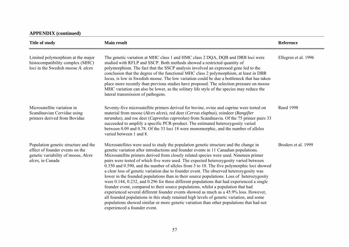
57


Title of study Main result Reference

Limited polymorphism at the major histocompatibility complex (MHC) loci in the Swedish moose A. alces

The genetic variation at MHC class 1 and HMC class 2 DQA, DQB and DRB loci were studied with RFLP and SSCP. Both methods showed a restricted quantity of polymorphism. The fact that the SSCP analysis involved an expressed gene led to the conclusion that the degree of the functional MHC class 2 polymorphism, at least in DBR locus, is low in Swedish moose. The low variation could be due a bottleneck that has taken place more recently than previous studies have proposed. The selection pressure on moose MHC variation can also be lower, as the solitary life style of the species may reduce the lateral transmission of pathogens.

Ellegren et al. 1996

Microsatellite variation in Scandinavian Cervidae using primers derived from Bovidae

Seventy-five microsatellite primers derived for bovine, ovine and caprine were tested on material from moose (Alces alces), red deer (Cervus elaphus), reindeer (Rangifier tarandus), and roe deer (Capreolus capreolus) from Scandinavia. Of the 75 primer pairs 33 succeeded to amplify a specific PCR-product. The estimated heterozygosity varied between 0.09 and 0.78. Of the 33 loci 18 were monomorphic, and the number of alleles varied between 1 and 8.

Røed 1998

Population genetic structure and the effect of founder events on the genetic variability of moose, Alces alces, in Canada

Microsatellites were used to study the population genetic structure and the change in genetic variation after introductions and founder events in 11 Canadian populations. Microsatellite primers derived from closely related species were used. Nineteen primer pairs were tested of which five were used. The expected heterozygosity varied between 0.350 and 0.590, and the number of alleles from 3 to 10. The five polymorphic loci showed a clear loss of genetic variation due to founder event. The observed heterozygosity was lower in the founded populations than in their source populations. Loss of heterozygosity were 0.144, 0.232, and 0.296 for three different populations that had experienced a single founder event, compared to their source populations, whilst a population that had experienced several different founder events showed as much as a 45.9% loss. However, all founded populations in this study retained high levels of genetic variation, and some populations showed similar or more genetic variation than other populations that had not experienced a founder event.

Broders et al. 1999

58



Monomorphism and polymorphism at Mhc DRB loci in domestic and wild ruminants

Moose from Sweden, Norway, Canada, and Alaska (a total of 256 individuals.) were analyzed using single strand conformation polymorphism (SSCP). The number of scored alleles was 6, 7, 4, and 3 for the respective countries, and He 0.76, 0.79, 0.59, and 0.31, respectively. The limited genetic variation of moose is notable in relation to the big population expansion that has been seen over the last 100 years. The authors raised the question of whether species or populations that have a limited MHC variation really have a weaker defense against infection diseases.

Mikko et al. 1999

Genetic relationships deduced from cytochrome-b sequences among moose

The nucleotide sequence variation of the mitochondrial cytochrome-b gene was examined. Haplotypes were generated for North American, Asian and European moose whilst three Eurasian haplotypes were obtained from GenBank. No nucleotide variation could be detected within the North American moose, whereas three haplotypes were found in European moose and four in the Asian moose. The low diversity of nucleotides in cytochrome-b indicates a recent ancestor of all moose of the world. The existence of a North American haplotype is a strong piece of evidence of a single and late entry into the New World via the Bering land bridge, instead of an entry at several occasions and through more than one corridor.

Hundertmark et al. 2002a

Mitochondrial phylogeography of moose (Alces alces): Late Pleistocene divergence and population expansion

The phylogeographic relationship among moose over the species geographic distribution range was investigated to answer the question if two geographical races really exist. The authors also tried to answer the timing and the sizes of the demographic processes that caused the expansion of moose over the Northern Hemisphere under the late Pleistocene period. The analyzed sequence (left hypervariable domain of the control region) showed low or moderate levels of variation worldwide and was structured geographically. Isolation by distance was the main factor that structured the moose populations at a regional scale, but it did not support the existence of distinct eastern and western races. Analyses identify Asia as the origin of all extant mitochondrial lineages, and that the population in Yakutia-Manchuria from eastern Asia was probably the source of the founders that colonized North America within the last 15 000 years.

Hundertmark et al. 2002b

59



Genetic diversity of moose (Alces alces L.) in Eurasia

Nucleotide sequences of D-loop of the mitochondrial DNA of moose from Eurasia, Sweden and North America were analyzed. Three main haplotype variants were found, which formed three geographic grouping that where called "European", "Asiatic" and "American".

Udina et al. 2002

Mitochondrial phylogeography of moose (Alces alces) in North America

The nucleotide sequence variation of a hyper variable domain of a mitochondrial DNA control region was analyzed to delineate the population structure of moose in North America. Altogether 16 haplotype variants were found, with the highest variation in the central part of the continent and the lowest in the peripheral populations. The result pointed towards a colonization pattern consistent with a central population that supplied founders to peripheral populations other than Alaska via long-distance dispersal rather than via a stepping-stone dispersal. The low haplotype variation in Alaska does not coincide with the colonization scenario (from Asia via the Bering land bridge about 14 000-10 000 years ago), and is probably due to a post-colonization bottleneck.

Hundertmark et al. 2003

Genetic variation and population structure of moose (Alces alces) at neutral and functional DNA loci

Mini and microsatellite markers and one MHC loci were used to examine the genetic variation and population structure of moose in nine Canadian areas of which three were national parks. The result showed that there were differences in allelic diversity between the neutral markers and MHC DRB locus in many of the populations. The population in Ontario showed high levels of genetic variation at the neutral markers whereas variation at the MHC DRB locus was relatively low. The convert pertains to the population on Isle Royale that had the lowest amount of genetic variation in the neutral markers of the nine geographic regions examined, which coincide with a former small founder event. The genetic variation at the MHC gene was, on the other hand, relatively high. Gene flow between some populations could also be demonstrated. At the microsatellite loci the expected heterozygosity varied between 0.378 and 0.610 and the number of alleles from 2.2 to 4.4.

Wilson et al. 2003

60



Population structure and genetic diversity of moose in Alaska

Genetic diversity and structure were studied using 141 moose from six regions spanning much of Alaska and eight polymorphic microsatellites. Expected heterozygosity were reported to be moderate (0.48-0.61) and private alleles ranged from 0 to 6. Significant population structure was detected using both FST (< 0.109) and RST (< 0.125). STRUCTURE results suggested two different groups, consisting of a mix of moose from Yakutat and Tetlin regions versus all other moose, with a slight substructure among the second population. A mantel test indicated that isolation-by-distance partially explained the observed structure among moose populations. No indications of bottlenecks were detected either at the population level or overall. The authors concluded that weak population structure occurs among moose in Alaska with a population expansion from interior Alaska westward toward the coast.

Schmidt et al. 2009

Genetic discontinuities in a continuously distributed and highly mobile ungulate, the Norwegian moose

The distribution of genetic variation, differentiation, and admixture were studied using 585 moose collected throughout Norway using 15 microsatellites. Using STRUCTURE without any geographic information suggested that the populations are divided into one southern and one northern subpopulation. Overall expected heterozygosity for the southern and northern population identified from STRUCTURE was 0.63 and 0.65, respectively. No bottlenecks or founder events were detected, but a high degree of private alleles were observed for the northern population suggesting introgression from populations from Sweden, Finland and Russia.

Haanes et al. 2011

Monitoring gene level biodiversity - aspects and

Documents

Transcript of Monitoring gene level biodiversity - aspects and