PROCEEDINGS, Thirty-Seventh Workshop on Geothermal Reservoir Engineering Stanford University, Stanford, California, January 30 - February 1, 2012 SGP-TR-194

MONITORING ENHANCED GEOTHERMAL FLUIDS WITH MAGNETOTELLURICS, TEST CASE: PARALANA, SOUTH AUSTRALIA.

1Jared Peacock,

1Stephan Thiel,

2Peter Reid,

2Mathieu Messellier and

1Graham Heinson

1University of Adelaide

Adelaide, South Australia, 5005, Australia 2Petratherm Ltd.

Unley, South Australia, 5061, Australia e-mail: jared.peacock@adelaide.edu.au

ABSTRACT

Realization of enhanced geothermal systems (EGS) prescribes the need for novel methods to monitor fluid inclusion and connectivity at depth. Magnetotellurics (MT) is a passive electromagnetic method sensitive to electrical conductivity contrasts as a function of depth. The goal here is to use MT as a monitoring tool to estimate areal extent of an EGS reservoir by collecting measurements before, during and after fluids are injected. 3D forward modeling suggests changes in the MT response will be small, on the order of a few percent. Repeatability of the MT response is important and it is shown that most stations are within a few percent. Results from a test case at Paralana, South Australia are presented supporting the idea that MT can be used as a monitoring tool by showing changes due to fluids input into the system.

INTRODUCTION

EGS is on the verge of becoming an economically viable solution to global clean renewable energy needs. Projects such as Soultz in France, Landau in Germany, and Cooper Basin in Australia are leading the way with many more projects in development. The Paralana EGS project run by Petratherm in the Northern Flinders Ranges of South Australia is preparing to drill the second of an injection/extraction doublet pair of wells. This comes after flow has been proven in a fracture stimulated zone. Reported here are results of MT surveys collected before and after the fracture stimulation showing changes in the response due to fluids being introduced into the system.

Enhanced Geothermal System

The idea of an EGS, first tested at Fenton Hill, NM in the 1970's, is relatively simple: introduce fluids into a zone of thermally active lithology via fracture stimulation, then extract the hot fluids to produce energy. This idea can be exploited anywhere

compliments of the natural thermal gradient in the Earth, with the typical target range for electricity generation being between 3 and 10 kilometers. Unfortunately, proving this idea as economically viable has been difficult with oil and gas prices still relatively low and anthropogenic environmental influence continuing to be a political issue. Nevertheless, the handful of EGS in operation such as Soultz, Landau, and the Cooper Basin are leading the way to economic viability. The first step to creating an EGS is fracture stimulation to establish porosity and more importantly permeability within the hot lithology. One problem that EGS needs to overcome is the uncertainty in how fluids connect within the lithology. The main geophysical technique to characterize fractures opening during the fracture stimulation is micro-seismic, however this is not directly sensitive to fluids being included in that fracture nor how well it is connected to other fractures. Electromagnetic (EM) techniques are directly sensitive to electrical conductivity contrasts, specifically connected paths of conductive material such as a brine solution.

Magnetotellurics

MT is a passive volumetric method that measures the Earth's electromagnetic response to natural time varying magnetic fields. As with most EM methods, MT is measuring a diffusive process, meaning that energy is only lost in the system and as a consequence the depth of penetration is time/frequency dependent--the longer the measurement the more sensitive to deeper structures

it becomes (1), where T is period and is resistivity. Furthermore, MT is a volumetric measurement that

incorporates the hemisphere of radius One unfortunate consequence of this is that resolution is also frequency dependent and decreases with increasing depth.

δ≈ 500√ρT (1)

To collect MT data in the field, two orthogonal horizontal components of both the electric and magnetic field are measured simultaneously for an extended period of time, dependent on target depth. The frequency dependent ratio of these fields results in the impedance tensor (1), which contains all the information about subsurface geoelectric structure.

E (ω)= Z B(ω) (2)

Two common ways to visualize the MT response is by computing the apparent resistivity (2) and the phase (3), where the subscript describes the

orientation of the electric and magnetic field and is the magnetic susceptibility of free space. The apparent resistivity is the volumetric resistivity of the

hemisphere described by radius and the phase is the phase of the impedance tensor component. Note that the phase predicts the apparent resistivity.

ρij(ω)=1

μoω∣E i(ω)

B j(ω)∣2

=1

μoω∣Z ij(ω)∣

2

(3)

ϕij(ω)= arctan(ℑm[ Z ij(ω)]

ℜ e [ Z ij(ω)]) (4)

Phase tensor

Another way to visualize the MT response is through the phase tensor, derived by Caldwell et al (2004). The phase tensor is the ratio of the real (X) and imaginary (Y) parts of the impedance tensor. One benefit of the phase tensor is that it is devoid of near surface distortions. The phase tensor can be graphically characterized as an ellipse with the long axis pointing in a direction of preferred current flow and oriented along geoelectric strike, with a 90 degree ambiguity.

ϕ=

X− 1

Y (5)

One reason for using MT to monitor an EGS system is that it is sensitive to conductivity contrasts. Here it is expected that the host rock will be resistive, on the order of a few hundred Ohm meters, and the fluid will be conductive, on the order of a few Ohm meters or less, due to dissolved ions and being thermally inclined. The contrast is a few orders of magnitude and can be measured down to depths of 10km.

FORWARD MODELING

To test MT as a viable method to monitor fluid inclusion at 4km depth 3D forward modeling was preformed. First, the MT response was calculated for a system similar to Figure 3 using the forward modeling code of Rodi and Mackie (2001). Then a block of .1 Ohm-m oriented in the NE direction with volumetric dimensions of 1km x 1km x 400m was introduced at 4km depth in a layer of 200 Ohm-m. The residual was then calculated between the MT response without and with a conductive block. The forward modeling reveals a change of a few Ohm-m in apparent resistivity, Figure 3, and about a degree in phase, Figure 4. One important result to observe is the period range in which the change occurs. In phase, the change occurs between .1 and 10 seconds and resistivity between 1 and 100 seconds. The unfortunate reality is that the source field of MT is naturally weak between 1 and 10 seconds increasing the importance of precise and accurate data when trying to estimate a change in the MT response.

Figure 1: Forward model apparent resistivity

calculated from the determinant of Z. Each plot is a map view of the residual between without and with a reservoir of conductive fluid. From left to right is increasing period, related to depth of penetration by (1). Red colors are large residuals and blues are small residuals. Here the largest change is about 10 Ohm-m in the period range of 10-100 seconds.

PARALANA, SOUTH AUSTRALIA

South Australia possesses some of the hottest granites in the world. Paralana, South Australia, is about 600km north of Adelaide in the Northern Flinders Ranges. Thermal activity is anomalously high within the crystalline rocks (heat flow of 60 mW/m

2) due to

a high density of radiogenic elements (Brugger et al. 2005). Interestingly, Paralana Hot springs is the only hot springs in the world heated by amagmatic activity.

Figure 2: Forward model impedance phase

calculated from the determinant of Z. Similar to Figure 3 where the change is now only about 1 degree. Note the change occurs are smaller periods supporting the idea that the phase predicts the resistivity.

At the Paralana drill site, the radiogenic crystalline basement is unconformably over laid by about 4500m of Adelaidian sediments acting as a thermal blanket creating a heat flow of about 113 mW/m

2 (Neumann

e al., 2000). Petratherm has drilled a well to 4012m which is cased to 3725m. Bottom hole temperature is estimated to be 190 C, while fluids were encountered at 3860m. The proposed reservoir will extend about 1km in the E-W direction, 1km in the N-S direction, 400 meters vertically and will be at about 3600m depth.

Fracture stimulation

In July, 2011 3.1 million liters of saline water (.3 Ohm-m) were pumped into the lithology via an 8m perforated zone around 3680m. Pumping lasted 5 days starting with low flow rates slowly increasing and periodically shutting in, Figure 2. A micro-seismic array measured over 13,000 events with 98% being less than magnitude 1.0. The seismic cloud shows the micro-fractures opening in a NE preferred direction and along an assumed preexisting fault system in the NE quadrant around the borehole. Two distinct main fractures seem to have been stimulated both oriented NE at slightly different angles. They are connected by an orthogonal fault about 400m from the borehole. The seismic cloud extends more than 1km NE and about 500m deep.

EXPERIMENT

With the goal of measuring a change in the MT response due to the inclusion of fluids, the plan is to measure before and after fluid injection by repeating the same survey multiple times. The survey has been designed as Figure 4 assuming the conductivity anomaly target to be around 4 km centered around

the Paralana 2 borehole. Each site is collected with two orthogonal induction coils and two dipoles oriented with magnetic North. A solar powered remote reference is place 60km south of Paralana operating over the entire survey period.

Figure 3: Cross section of Paralana, South Australia. Paralana 1 was an exploration hole, Paralana 2 is the injection well. The fracture stimulation occurred at about 3680m just above the hot granites.

DATA

Multiple base surveys were collected to get accurate and precise data to compare with post injection data. Each station was collected with a sampling rate of 500 Hz and an electrode spacing of around 50m. Each MT station was processed using a bounded influence robust remote reference processing code developed by Chave (2004). Furthermore, each station that was collected at different times were processed with the same parameters to insure no influence from the processing code.

Figure 4: MT survey design centered on Paralana 2 borehole. Two orthogonal lines oriented along existing seismic lines N-S and E-W. Two off diagonal lines help constrain 3D effect. Spacing starts at 200m near the borehole and increase to 1.5km near the edges.

Figure 5: Plot of pumping rate during fracture

stimulation. Red is flow rate and blue is well head pressure as a function of time.

Base Survey

Four different base surveys were collected due to varying data quality. The first survey in March 2010 employed metal stakes as electrodes which randomly worked well for some sites but not others. Cu-CuS04 electrodes were used for all other surveys. Those sites that did not work were repeated during the second survey in May 2010. Unfortunately, the EPIC pipeline, running parallel to the N-S line offset 1km to the west, was performing its annual corrosion test by sending a 3 second square wave pulse every 12 seconds, saturating the MT data in the period range of 1-12 seconds and harmonics of 12 seconds. This was removed by subtraction of a data driven replication of the pipeline noise, Figure 6. The entire survey was repeated in March, 2011, where the pipeline was again producing a signal but the magnitude was similar to the MT signal. The same time series processing technique was applied. 11 sites around the borehole were collected a few days before the injection test to give an estimate of any changes in the subsurface directly before the injection. Inversions of the data were conducted employing the Occam inversion code developed by Constable et al. (1987) and the conjugate gradient method developed by Rodi and Mackie (2001). The Occam inversion are shown here to display the simplest model possible, Figure 7 and Figure 8. Three important observables arise. First, the top 500-1000m are highly conductive, 1-10 Ohm-m, which is important because the skin depth is dependent on the resistivity. The less resistive the material the shallower the EM energy will penetrate. Second, conductive wedges are bounded by faults interpreted from seismic data suggesting either a fluid filled fault system or mineralization of the faults due to ancient fluids. Third, the resistivity of the proposed reservoir is on

the order of a few hundred Ohm-m, meaning the contrast between conductive fluids will be 2 orders of magnitude.

Figure 6: Data driven noise removal. Top) the

result of removing the periodic signal. Middle) black is the raw data and red is the data driven periodic time series. Bottom) spectrum of the raw data and filtered data.

Post Injection

One week after the injection the full survey was repeated. The pipeline was not producing a significant signal so the instruments were deployed for an average of 20 hours. Repeating the sites exactly as originally deployed was relatively easy as the disturbed top soil from the covered coil holes and electrode holes was still visible from the surface at most sites. Due to an unusual amount of rainfall the vegetation was overgrown leading to a mouse infestation during the austral winter. Unfortunately, mice like to chew the electrode cables so some sites lasted about 10-15 hours instead of the full 20, and some sites had to be completely redone due to chewed cables.

RESULTS/DATA ANALYSIS

As already mentioned the data were processed using the code developed by Chave et al. (2004) in advanced mode. Here coherence thresholds can be placed on the magnetic and electric fields separately cleaning up the dead band. The same parameters were used for each repeated station to remove any bias developed by processing with different parameters.

Repeatability

One important parameter to evaluate when comparing data from different surveys is measurement repeatability. Multiple base surveys were collected and multiple measurements at the

same station were collected allowing repeatability estimation. This can be calculated as a percentage difference between one measurement and another for apparent resistivity and phase. Care must be taken when comparing the resistivity due to the influence of near surface distortions. One way to remove the distortion is described by Bibby et al. (2005). A simpler method would be estimating the repeatability by calculating the phase tensor difference (6) derived by Heise et al., (2007), where I is the identity matrix

and is (5). Again, the advantage of the phase tensor is that it is devoid of near surface distortions such as static shift.

Figure 7: Occam inversion of EW profile from base survey, left is west and right is east. Paralana 2 is marked by the black line in the middle of the profile. Notice the top 1km is highly conductive, the conductive wedge around the borehole bounded by faults interpreted from seismic and the large conductive body at 11km.

Figure 8: Occam inversion of NS profile from base

survey, left is south and right is north. Paralana 2 is marked by the black line in the middle of the profile.

Plotting (6) as an ellipse is displayed in Figure 9. It is evident that repeating measurements at the same site is accurate for the band (.01-2 sec). However, in the dead band (2-15sec) the accuracy of repeating a measurement decreases, which is unfortunate because this is the target band for signal arising from fluid inclusion.

Δ= I− (ϕ2− 1ϕ1+ ϕ1ϕ2

− 1)/ 2 (6)

Figure 9: Phase tensor repeatability. For selected

stations with repeated measurements, the phase tensor difference was calculated using (6). The size is in degrees and is related to magnitude difference between measurements. Notice the size and orientation varies in the dead band (1-15sec).

Table 1: Repeatability estimations (%) for different

MT parameters in two different period ranges.

MT Parameter T=0.01-1 (s) T=1-200 (s)

a 2.17 9.43

0.97 5.55

Det{} 1.64 6.77

Before and After Comparison

Multiple methods can be employed to compare the MT response before and after fluids are injected into the system. The simplest is to compare the curves of apparent resistivity and phase of the before and after measurements, Figure 10. Again, comparing the

apparent resistivity needs to be done with care so as to remove distortions caused by near surface inhomogeneities. Here the distortion has been removed using the method described in Bibby et al. (2005) and then the curves are matched at short periods by removing the static shift between measurements. It is assumed that the near surface has not been changed by fluids being injected at 3600m. This simple comparison shows that the changes are small on the order of a few percent which is right in the repeatability range and noise level. Another method is to calculate the phase tensor determinant which is not only insensitive to near surface distortions but also misalignment of the magnetic coils. Plotting this up as a map for each period reveals changes in the phase tensor determinant comparing before and after fluids are introduced.

Figure 10: Comparing apparent resistivity and phase before and after fluids are injected into the system. Blue and red curves are before, cyan and magenta are curves after. Top) Log apparent resistivity with near surface distortion removed. Note the change around 10-30 seconds. Bottom) impedance phase, notice the change around 1-4 seconds.

DISCUSSION

The micro-seismic data collected during the injection suggests that the fractures opened up in a NE orientation with the majority of fractures in the NE quadrant around the borehole. With this information care must be taken when interpreting changes in the MT response for repeated surveys. Repeating measurements in the dead band proves to be more difficult than other period ranges, Table 1. Changes in the determinant of the phase tensor reveals changes in the dead band around 8-9 percent which is more than the repeatability error, suggesting changes observed are due to the subsurface changes and not changes due to noise. Nevertheless it is important to locate sources of noise to give confidence to results. One obvious source of

noise is the EPIC pipeline. Fortunately, this noise signal is regular and can be accurately extracted from the data. Poor source signal strength in the dead band can cause larger error bars in impedance estimation giving a false anomaly. Not repeating the exact same station can cause some error. For example if the same instruments are not used, the electrodes are placed in a different place, the magnetic coils are oriented slightly off angle of the previous measurement, mice chewing cables, wind blowing cables around or vegetation growth. Fortunately, using the phase tensor determinant is insensitive to most of those parameters. Calibration of the induction coils is important to make sure there is no change due to instrument response. Seasonal changes in the subsurface can generate a change in the MT response. 2010 was an unusually wet year for South Australia, however these changes normally occur in the top kilometer and the repeatability in this period range implies little change in the subsurface due to seasonal changes with one exception. To the west of the borehole appears a conductive anomaly in the same location as a fault interpreted from seismic, suggesting fluids from excessive rain fall have migrated into this fault system. This could also be part of the natural water cycle which will be important in determining the extraction well location. Along with the aforementioned sources of noise, one thing to keep in mind when interpreting Figure 11 is that the images are produced using a nearest neighbor interpolation scheme to build the image matrix, which tends to smear anomalous points, especially when the nearest neighbor is far away as around the edges. Then a bicubic interpolation is used to smooth the image. Forward modeling suggests that the conductive anomaly should occur in the period range of .1-5 seconds and data from the micro-seismic array demonstrates the fractures opened up in the NE quadrant around the borehole in a NE orientation. The first thing to notice is that the 200m immediately surrounding the borehole there exists a resistive anomaly for most periods. This could be due to fresh water mixing in with saline fluids. The fluid pumped into the formation was saline implying that preexisting fluids are less saline. The unanswered question is: where did that fresh water come from? If it came from the formation, it must have come from deeper than the injection because the fluid encountered above the perforation zone during drilling is conductive. The next anomaly to notice is to the conductive body immediately to the east of the resistive circle for periods from 1-16 seconds, being prominent at 6 seconds. This body coincides with data from micro-seismic and could be the reservoir of saline fluids that were pumped into the formation. It is important to

realize that the resolution of MT at depths of 4km will be on the order of a few hundred meters, therefore a small conductive body will be smeared out and poorly resolved. However, MT can resolve the depth to the top of the conductor well, which is similar to the depth derived from micro-seismic data. Another characteristic of MT to keep in mind is that it is more sensitive to conductive bodies than resistive bodies. An interesting observation is that the reservoir did not spread like a disc symmetrically around the borehole but in a preferred direction and not just horizontally but vertically as well. Location of the primary resistive and conductive features moves around with increasing depth, demonstrating the complexity of the reservoir and fracture system. The conductive body to the west of the borehole for periods of .6-2 seconds is either due to noise or more likely a fluid filled fracture due to rain water drainage.

CONCLUSIONS

This pilot study suggests that MT can be used as a monitoring tool for EGS and other fluid injection processes. Repeating measurements before and after fluids are injected is logistically favorable but introduces some noise. Estimating the phase tensor determinant is insensitive to most of these noise sources. When interpreting the data other sources of noise need to be taken into account, such as pipeline noise, source field noise, and wind noise. Accurate and precise data is of utmost importance, especially in the MT dead band. The unfortunate reality of passive measurements dependent on natural fields is that the operator has no control over the strength, frequency or polarization. Therefore, it has been suggested that controlled source EM should be used for monitoring surveys. However, getting energy down to depths of 4km with a conductive overburden can prove to be difficult. A down hole EM source could be a good option. The most important property of an EGS reservoir is the connectivity or permeability of the fracture system. MT cannot directly measure the permeability but it can infer volumetric electrical connectivity interpreted as fluid filled fractures. MT measures volumetric geoelectrical structures, by increasing the station density resolution increases. Future surveys should have denser station spacing and coverage. Another survey a few months after the injection could give more information about the reservoir after it has reached equilibrium.

ACKNOWLEDGMENTS

The authors would like to thank Petratherm and joint venture partners Beach Petroleum and TruEnergy for support of this project. Goran Boren, Jonathan Ross, Hamish Adam, Tristan Wurst, Kiat Low, Aixa Rivera-Rios, Alison Langsford, and Kathrine Stoate for field work assistance. Also, IMER, South Australian Center of Geothermal Energy Research (SACGER) and PirSa for financial support.

REFERENCES

Bibby, H. M., Caldwell, T. G., & Brown, C. (2005), “Determinable and non-determinable parameters of galvanic distortion in magnetotellurics,” Geophys. J. Int., 163, 915-930.

Brugger, J., Long, N., McPhail, D. C. & Plimer, I. (2005), “An active amagmatic hydrothermal system: the Paralana hot springs, Northern Flinders Ranges, South Australia,” Chemical Geology, 222, 35-64

Caldwell, T. G., Bibby, H. M., Brown, C. (2004), “The magnetotelluric phase tensor”, Geophysical Journal International, 158, 457-469

Chave, A. D. & Thomson, D. J. (2004), “Bounded influence magnetotelluric response function estimation,” Geophysical Journal International, 157, 988-1006

Constable, S. C., Parker, R. L., Constable, C. G. (1987), “Occam's inversion: A practical algorithm for generating smooth models from electromagnetic sounding data,” Geophysics, 52, 289-300

Heise, W., Bibby, H. M., Caldwell, T. G., Bannister, S. C., Ogawa, Y., Takakura, S., Uchida, T. (2007), “Melt distribution beneath a young continental rift: the Taupo Volcanic Zone, New Zealand,” Geophysical Research Letters, 34, L14313, doi: 10.1029/2007GL029629.

Neumann, N., Sandiford, M. & Foden, J. (2000), “Regional geochemistry and continental heat flow: implications for the origin of the South Australian heat flow anomaly,” Earth and Planetary Science Letters , 183, 107-120

Rodi, W. and Mackie, R. L. (2001), “Nonlinear

conjugate gradients algorithm for 2-D magnetotelluric inversion,” Geophysics, 66, 174-187.

Spichak, V.V., and Manzella, A (2009), “Electromagnetic Soundings of Geothermal Zones”, Journal of Applied Geophysics, 68, 459-478

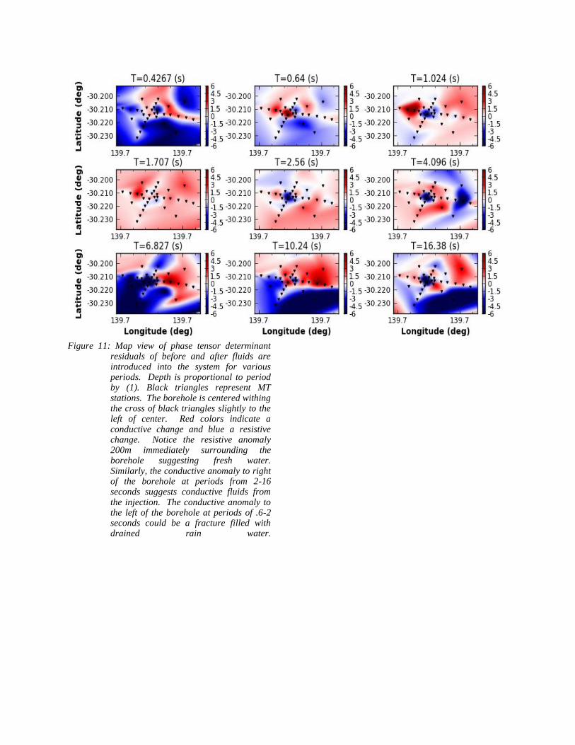
Figure 11: Map view of phase tensor determinant residuals of before and after fluids are introduced into the system for various periods. Depth is proportional to period by (1). Black triangles represent MT stations. The borehole is centered withing the cross of black triangles slightly to the left of center. Red colors indicate a conductive change and blue a resistive change. Notice the resistive anomaly 200m immediately surrounding the borehole suggesting fresh water. Similarly, the conductive anomaly to right of the borehole at periods from 2-16 seconds suggests conductive fluids from the injection. The conductive anomaly to the left of the borehole at periods of .6-2 seconds could be a fracture filled with drained rain water.