Monetary Union Begets Fiscal Union

Adrien Auclertaauclert@mit.edu

Matthew Rognlie∗

mrognlie@mit.edu

August 2014

Abstract

We propose a mechanism through which monetary union between countries leads to astronger fiscal union. Although fiscal risk-sharing is valuable under any monetary regime,given nominal rigidities it is more important within a monetary union, when exchange ratescan no longer adjust to offset shocks. As a result, countries in a monetary union are capableof achieving better risk-sharing, partly overcoming their lack of commitment. Still, equilibriawithout fiscal cooperation remain possible and imply inefficient cross-country dispersion inoutput. A proactive central bank can encourage transfers by providing extra accommodationwhen fiscal union is under stress.

Transfer criterionCountries that agree to compensate each other for adverse shocks form an optimum currency area.

Baldwin and Wyplosz (2012), Chapter 15

1 Introduction

A simplified narrative of the recent crisis in the Eurozone can be given as follows. Following theadoption of the single currency, a number of “periphery” countries progressively lost competitive-ness as their real unit labor costs grew faster than the union average. When the global financialcrisis hit in 2008, the accumulated internal imbalances came into sharp focus. Given their fixednominal exchange rate vis-à-vis other Eurozone members, the only way periphery countries couldachieve the real depreciation needed to regain competitiveness was through a painful process ofeconomic contraction bringing about falls in domestic prices. Indeed, this adjustment processwas so damaging to periphery economies that there was mounting speculation that some of themmight leave the Euro. Monetary union was under stress. But it ultimately did not break: Eurozone

∗We thank Iván Werning for continued encouragement and many useful suggestions. We also thank ArnaudCostinot, Emmanuel Farhi, Vincent Pons, Alp Simsek, Daan Struyven, Robert Townsend, and participants at the MITInternational Lunch for helpful comments. Remaining errors are our own. Adrien Auclert gratefully acknowledgesfinancial support from the Macro-Financial Modeling group.

1

countries were strongly bound to their single currency despite the large stabilization costs that itinduced.

Meanwhile, periphery countries’ large external and fiscal deficits became increasingly difficultto finance. Some of the financing was bridged through bailout packages, but their size was limitedby reluctance from core country taxpayers who were supposed to fund them. Eurozone fiscalunion was only implicit, and core countries hit their participation constraint.

Our paper studies fiscal unions subject to such participation constraints, contrasting their roleinside and outside a monetary union. To capture features of fiscal union that resemble those of theEurozone today, we assume that countries have limited ability to commit to risk-sharing. Specifi-cally, we require that cross-country transfers always be part of a subgame-perfect equilibrium of arepeated game: in our model, countries only make transfers if these transfers are backed by cred-ible promises of future reciprocity. This emphasis on reciprocity is supported by a recent studyfrom the IMF (Allard et al. (2013)), which finds that “with a risk-sharing mechanism in place overa sufficiently long period, all current euro area members would have benefited from transfers atsome point in time”. Meanwhile, we capture the costs of monetary union by introducing nominalrigidities. When countries are part of a monetary union, the central bank can stabilize the unionas a whole, but not each individual country—leading to overheating in some countries and to re-cessions in others. These stabilization costs are absent under independent monetary policy, whereeach country’s central bank can stabilize its own economy separately.

Our primary result is that monetary union enhances fiscal union. The stabilization costs in-duced by monetary union also make countries more willing to share risks. This is due to an inter-action between the degree of risk-sharing and the ability of the union-wide central bank to stabilizeits members: when countries share risks better, there is less divergence in the stance of monetarypolicy that is appropriate for each country individually. In our benchmark model, this idea is il-lustrated starkly by the risk-sharing miracle: when its member countries share risks perfectly, theunion-wide central bank is able to stabilize all of them simultaneously.

Our paper proposes a mechanism through which monetary union between countries leads toa stronger fiscal union. By doing so, it contributes to sequencing theory, a field of international rela-tions that studies how one type of economic cooperation can lay the foundation for the next. Thisliterature often takes as a starting point an interpretation of Balassa (1962), according to whichregional integration takes place by progressively climbing the steps of the “integration staircase”depicted in figure 1 (Gustavsson (1999), Estevadeordal and Suominen (2008), Baldwin (2012)).Central to sequencing theory is the existence of spillovers that make integration gather momen-tum by begetting further cooperation in other areas. For example, Haas (1958), in his famousstudy of the European Coal and Steal Community in the early 1950s, emphasizes the ability of thenewly-founded institution to support special interest groups that pushed for broader economicintegration, eventually leading to the European Economic Community. Our paper microfoundsthe spillovers that enable countries to climb the last step of the integration staircase: in a mone-tary union, the absence of fiscal union becomes more costly, and countries internalize this when

2

deciding on fiscal cooperation.

Each country for itself

Free Trade Area

Customs Union

Common Market

Monetary Union

Fiscal Union

Figure 1: The integration staircase

Our paper also adds to the theory of Optimum Currency Areas (Mundell (1961), McKinnon(1963), Kenen (1969)) by proposing a new tradeoff, between stabilization costs and risk-sharingbenefits of monetary union. While the cost side of the ledger—the difficulty of monetary union tocope with asymmetric shocks—has been well understood since at least Friedman (1953), the ben-efit side has lacked comparatively compelling microfoundations. The literature emphasizes suchdiverse advantages as the elimination of transactions costs or the gains from reduced uncertainty,which we find less tangible than the risk-sharing benefits stressed in this paper. Another recentpaper revisiting the benefits side of the monetary union ledger is Chari, Dovis and Kehoe (2013).Their emphasis is on the benefits to central bank credibility, pointing out that a union may reduceoverall inflationary bias to the extent that the shocks that create a desire to inflate are not perfectlycorrelated across countries. This channel is absent in our model, in which we shut off all forms ofinflationary bias.

One way to read our paper is thus, in the light of the OCA literature, as a direct argumentfor why countries might form monetary unions despite their apparent costs. Our argument isthat these costs may in fact be the seed of the benefits: once the monetary union is joined, thepossibility of high stabilization costs in the absence of fiscal cooperation enforces the cooperationitself, and limits the incurrence of the costs.

Having established our main result, we go further and ask what the union-wide central bankcan do, given additional commitment power, to proactively encourage the fiscal union. We findthat it can help, by departing from its traditional role of aggregate stabilization and committing toaccomodative monetary policy in volatile times. Accomodative monetary policy helps because itcreates an overall boom in the union, which in turn effectively relaxes countries’ participation con-straints and facilitates transfers. This incentive effect is new to the literature on optimal monetarypolicy in currency unions.

Our model puts together two distinct strands of the literature. The first is the literature onlimited commitment (Kehoe and Levine (1993), Coate and Ravallion (1993), Kocherlakota (1996),

3

Alvarez and Jermann (2000), Ligon, Thomas and Worrall (2002)). This literature derives endoge-nous constraints on risk-sharing by giving agents the option to leave transfer arrangements at anypoint in time, and it focuses on the best outcomes that are sustainable given these constraints.When countries run an independent monetary policy, our setup reduces to the one described bythis literature, and the same forces—the degree of patience, risk-aversion, and the persistence ofthe idiosyncratic endowment processes—drive the feasible amount of risk-sharing.

We combine the constraints on risk-sharing featured by the limited commitment literature withthe constraints on monetary policy emphasized by the modern international economics litera-ture on currency unions in the presence of nominal rigidities (Benigno (2004), Galí and Monacelli(2005), Galí and Monacelli (2008)). This literature provides a microfoundation for the stabilizationcosts that arise in currency unions, as the central bank is generally unable to fully stabilize eachmember country and must balance out the cross-country distortions it creates by setting its policyinstrument at an intermediate level.

Our paper is close in spirit and in form to Farhi and Werning (2013), who also study the bene-fits of a fiscal union of the kind we describe — cross-country insurance arrangements — within amonetary union. While they focus on the constrained inefficiency of private arrangements and theneed for government interventions to reach a constrained-optimal outcome, we shut off privateinternational financial markets and study a constraint faced by the governments in their imple-mentation of the optimal outcome. In doing so, we extend their framework to allow for a fullgame-theoretic analysis of monetary and fiscal policy. In most of our paper, the risk-sharing mira-cle holds and the constrained-optimal outcome is also first-best, a case which is of limited interestin Farhi and Werning (2013), but which we regard as capturing in an elegant way the widespreadview that alignment of fiscal policy limits the costs of monetary union. Under the risk-sharing mir-acle, nominal rigidities only create a cost to the extent that a limited commitment friction bindsand prevents countries from reaching a full risk-sharing outcome. As we briefly discuss, thiswould no longer be true if we allowed for shocks to preferences or nontradables productivity.

Another paper that discusses monetary union in the presence of a limited commitment frictionis Fuchs and Lippi (2006). Their focus is on the short-term commitment benefits brought about bymonetary union, in a situation where independent central banks might otherwise be tempted tofollow beggar-thy-neighbor policies. They use a reduced form to specify country preferences overthe level of the monetary policy instrument. In contrast, we abstract away from the interestingpossibility that monetary union might break up, but we fully endogenize fiscal and monetary pol-icy, assuming both policies maximize country welfare subject to the constraints of the environment(limited commitment and nominal rigidities). This allows us to study the rich ways in which thesetwo frictions—and these two types of policies—interact.

Many recent policy discussions have been focused on the need to establish fiscal federalism inthe Euro Area. Our model recognizes the importance of these efforts. Except in the special casewhere our mechanism is so powerful as to endogenously lead countries to share risks perfectly,the limited commitment friction does create costs, so it is valuable to try and mitigate it. In fact,

4

the risk-sharing miracle implies that if countries could overcome the commitment friction alto-gether, they would be able to attain the first best. In practice, it has been difficult to get countriesto sign formal agreements regarding contingent future fiscal transfers. We have two insights toadd here. First, we emphasize that because it is in the private interest of countries to internalizethe macroeconomic externalities associated with monetary union (Farhi and Werning (2013)), astronger fiscal union might emerge on its own: the set of possible equilibria is enlarged, thoughcountries may take time to move to the more cooperative one. Second, our normative analysissuggests that proactive monetary policy might be used as an imperfect substitute to fiscal union,nudging countries into sharing risks better.

The rest of our paper is organized as follows. Section 2 introduces our main framework, layingout our model’s game-theoretic foundations and defining our equilibrium concept. It then provesa number of properties of equilibria which simplify the analysis in the rest of the paper. Amongthese are the risk-sharing miracle (Theorem 1) and the ability to sustain any subgame perfectequilibrium using strategies that revert to autarky following any deviation (Theorem 2). Section 3considers a case where countries’ endowments satisfy a simple symmetry condition, and deliverstwo main results that substantiate our claim that monetary union enhances fiscal union. Theorem3 shows any risk-sharing arrangement that is sustainable under independent monetary policyis also sustainable under monetary union. It is a sharp illustration of the sense in which themonetary union improves risk-sharing. Theorem 4 shows that, under certain cases, the monetary-union-induced improvement in risk sharing is so powerful that it can take countries all the wayfrom autarky to first best. Section 4 proposes a normative analysis of monetary policy when fiscalunion is subject to a limited commitment friction. Theorem 5 shows that it is valuable to provideaggregate stimulus in times of high volatility in order to create a macroeconomic environmentfavorable to transfers between countries. Section 5 concludes. All proofs are in Appendix A.

2 Main framework

2.1 Fundamentals

Two countries i = 1, 2 live forever and have identical preferences. Each values the stream oftradables consumption

{Ci

T,t

}, nontradables consumption

{Ci

NT,t

}and labor

{Ni

t}

according tothe utility function

E

[∞

∑t=0

βtu(

CiT,t, Ci

NT,t, Nit

)]where we specify the felicity function to be log in tradables and nontradables, and isoelastic inlabor:

u (CT, CNT, N) = log (CT) + α

(log (CNT)−

N1+φ

1 + φ

)(1)

All goods are perishable, tradables goods are nonproduced, nontradable goods have to be con-sumed where they are produced, and labor is immobile across countries.

5

There exists another country in the world that is also endowed with tradables. The only pur-pose of this country in the model is to provide the reference unit of account, as Section 2.1.3 willdiscuss.

2.1.1 Tradable goods

Aggregate uncertainty is decribed by a finite-state Markov process {st} with elements st ∈ S andtransition matrix Π. A history of length t is denoted by st = (s0, . . . , st). We write sτ � st toindicate that sτ is a successor node of st.

Each country has a risky endowment EiT (st) of an identical, freely tradable good. The aggre-

gate state st thus determines the distribution of tradable endowments across the two countries.For now, tradable endowment shocks are the only source of uncertainty in the model.

Assumption 1 (External balance). The union achieves external balance in each history st:

C1T(st)+ C2

T(st) = E1

T (st) + E2T (st) ≡ ET (st) ∀st = (s0, . . . , st)

Assumption 2 (Strict benefits from tradables risk-sharing). For all s ∈ S, there exists s′ ∈ S such that

E1T (s)

E2T (s)

6= E1T (s′)

E2T (s′)

Since countries have concave expected utility over tradable consumption, assumptions 1 and 2together imply that there exist ex-ante utility gains from sharing risks by arranging state-contingenttransfers of tradables. Like Farhi and Werning (2013), we call such an arrangement a “fiscalunion”. In our model, the extent of risk-sharing is limited by a commitment friction which wewill soon describe.

2.1.2 Nontradable goods

Nontradable goods are produced from labor by a continuum of firms. We abstract from uncer-tainty regarding nontradable production, and discuss the consequences of relaxing this assump-tion in Section 3.3. In each country i, there is a continuum of firms j ∈ [0, 1] that each operate thesimple technology

Yi,jNT = Ni,j

in each period1. The consumer’s utility value from the consumption of each variety is given bythe CES aggregator

CiNT =

(∫ 1

j=0

(Ci,j

NT

) ε−1ε dj

) εε−1

ε > 1 (2)

1To reduce notation, we suppress dependence on the time and state whenever this is unambiguous.

6

Consumption of each variety must equal production, Ci,jNT = Yi,j

NT, and labor market clearing re-quires Ni =

∫j Ni,jdj.

Our assumed preferences and production structure are intended to make the first-best level ofnontradables a simple reference point. Since all firms have the same technology, efficiency requiresthem to produce equally, in which case Ci,j

NT = Ni,j = CiNT = Ni for all j. Optimizing utility (1)

subject to this constraint gives CiNT = Ni = 1.

Lemma 1. An efficient allocation of production requires Ci,jNT = Ni,j = 1, ∀i, j

In equilibrium, production may depart from this efficient level as a result of monopoly powerand nominal rigidities.

2.1.3 Rest of the world and units of account

In order to discuss exchange rate regimes, we need to be specific about units of account. We as-sume that the homogenous tradable good is traded as part of a world market, and that its foreign-currency price is normalized to P∗T

(ht) = 1 in all histories ht (ht consists of the exogenous state st

as well as the history of previous actions by all agents, as described below). The foreign currency,which we call the dollar, then provides a natural reference unit of account, and we assume thattransfers between countries are specified in that unit of account. With this interpretation, assump-tion 1 amounts to imposing that the two countries have a closed capital account vis-à-vis the restof the world.

We think of monetary policy as fixing the nominal exchange rate E i (ht) in each history—thatis, the number of units of domestic currency it stands ready to buy or sell per dollar. By the law ofone price for tradables, the exchange-rate policy of the central bank effectively fixes the domesticcurrency price of the tradable good at Pi

T(ht) = E i (ht) in every history ht. The key difference

between flexible exchange rates and a monetary union is that, in the latter, the union-wide centralbank has to set a common exchange rate E1 (ht) = E2 (ht) in each history.

2.2 Timing and equilibrium

As ensured by Assumption 2, there are gains from risk-sharing in tradable goods. We study an en-vironment where transfers between countries emerge as part of a subgame perfect equilibrium ofa repeated game. Three distinct types of actors participate in this game: monopolistically competi-tive firms setting prices for nontradable goods, fiscal authorities for each country, and—dependingon the monetary regime—either a common central bank for both countries or two independentcentral banks.

The timing within each period is given in Figure 2. We start by outlining the sequence of eventsinformally, before describing each part in detail in Sections 2.2.1-2.2.4.

7

(ht−1)

Producers set PiNT

st realized

Governmentsset transfers T1, T2

Monetary policy sets E i

End-of-periodequilibrium

(ht)

Figure 2: Timing

At the beginning of period t, ht−1 includes the history of all previous actions and states. Eachactor in period t has a pure strategy conditional on both the incoming history ht−1 and any preced-ing actions within period t. First, before the state is realized, firms set nontradable goods prices(in the domestic unit of account) based on ht−1, producing a price distribution ϕi

t in each country.Once the state st is realized, the fiscal authority in each country makes a transfer Ti based on ht−1,{ϕi

t}, and st. As discussed in Section 2.1.3, this transfer is specified in the international unit ofaccount. Next, exchange rates E i

t are chosen either separately in each country or—in the case ofa monetary union—commonly for both, based on ht−1, {ϕi

t}, st, and {Tit}. Finally, based on the

state and all actions thus far in the period, the end-of-period market determines production andconsumption according to household demand.

In the following sections, we proceed by backward induction, describing how the outcome ateach step within the period is determined, taking subsequent strategies as given. As depicted inFigure 2, there are four steps of interest: end-of-period equilibrium, monetary policy, fiscal policy,and pricesetting. These are the subjects of Sections 2.2.1-2.2.4, respectively.

2.2.1 End-of-period equilibrium

Households. At the end of the period, households in country i are faced with prices Pi,jNT, Pi

T,and W i, as well as profits ψi,j earned from each firm j’s production and a lump sum tax ti fromthe domestic government. The nontradable goods prices Pi,j

NT have already been set, while theprices Pi

T and W i are determined on a Walrasian market. We assume that households do not haveaccess to financial markets. We could allow them to access domestic financial markets without lossof generality: since the government has access to a lump-sum tax, Ricardian equivalence wouldhold.

Households optimally choose consumption

{Ci

T, Ci,jNT, Ni

}∈ arg max{

CiT ,Cij

NT ,Ni}(

log(

CiT

)+ α

(log(

CiNT

)−(

Ni)1+φ

1 + φ

))

s.t. PiTCi

T +∫ 1

j=0Pi,j

NTCi,jNTdj ≤ Pi

TEiT + W iNi +

∫ 1

j=0ψi,jdj− ti (3)

where CiNT is the aggregator in (2). The following lemma is derived from the first-order conditions

of the problem.

Lemma 2. At an optimum of the consumer problem, tradable and nontradable consumption are propor-

8

tional:

CiNT = α

PiT

PiNT

CiT (4)

good-specific non-tradable demand is

Ci,jNT =

(Pi,j

NT

PiNT

)−ε

CiNT (5)

and labor supply is

Ni =

(W i

PiNT

1Ci

NT

) 1φ

(6)

where PiNT =

(∫j

(Pi,j

NT

)1−εdj) 1

1−ε

is the price index associated with{

Pi,jNT

}.

Profits of nontradable goods producers. We assume that governments subsidize the labor costof firms at a rate τi

L = − 1ε . Given its price Pi,j

NT, producer j honors demand Ci,jNT by hiring Ni,j

workers and generates profits

ψi,j =(

Pi,jNT −

(1 + τi

L

)W i)

Ni,j (7)

which are remitted to households as part of their budget (3).

Government. As determined earlier in the period, the government of country i sends an inter-national transfer of Ti and receives one of T−i, both denominated in dollars. It operates the labortax, and rebates all profits to households. Its budget constraint, expressed in domestic currencyunits, is then

ti = E i(

T−i − Ti)+ τi

LW i∫

jNi,jdj (8)

Law of one price for tradable goods. As per its decision earlier in the period, the central banksets its nominal exchange rate E i against the dollar. Given this exchange rate, domestic residentscan purchase tradable goods from the rest of the world at price E i or from the domestic market atprice Pi

T. Equilibrium requires that the two be equated, to prevent pure arbitrage profits:

PiT = E i (9)

Market clearing for labor. Each firm hires to meet demand based on the price it posted. A firmwith posted price Pi,j

NT must hire

Ni,j = Yi,jNT =

(Pi,j

NT

PiNT

)−ε

CiNT (10)

9

where CiNT is country i’s aggregate nontradable demand. Labor market clearing requires that

Ni =∫

jNi,jdj = ∆i

NTCiNT (11)

were ∆NT ≡∫

j

(Pi,j

NTPi

NT

)−ε

dj ≥ 1 is a measure of price dispersion.

Indirect utility function. Conditional on the state and realized actions earlier in the period, end-of-period equilibrium is a nominal wage W i, a tradables price Pi

T, household quantities{

CiT, Ci,j

NT, Ni}

,

firm quantities{

Yi,jNT, ψi,j, Ni,j

}and a domestic government transfer ti, such that household opti-

mization conditions (4)-(6) are satisfied, household budgets are balanced (3), the law of one price(9) holds, firms produce to meet customer demand according to (10) and generate profits (7), thegovernment balances its budget (8), and the labor market clears (11).

Lemma 3. Given {ϕi}, s, {T1, T2}, E i, end of period equilibrium is unique. The nontradable price indexand price dispersion are given by

PiNT =

(∫p1−εdϕi(p)

) 11−ε

; ∆NT =∫ ( p

PiNT

)−ε

dϕi(p)

Country i consumes tradablesCi

T = EiT (s) + T−i − Ti

while on the nontradable side its production, consumption, and labor are given by

YiNT = Ci

NT = αE i

PiNT

CiT; Ni

T = αE i

PiNT

∆iNTCi

T

The country attains indirect utility

vi({ϕi}, s, {T1, T2}, E i) = log(

CiT

)+ α

log

(αE i

PiNT

CiT

)−

(α E

i

PiNT

∆iNTCi

T

)1+φ

1 + φ

(12)

If we define Vi(ht−1) to be the expected utility of a country starting at history ht−1, the follow-ing recursion holds, leaving dependence of equilibrium objects on history implicit for simplicityof notation:

Vi(ht−1) = ∑st

π(st|st−1)(

vi({ϕit}, st, {T1

t , T2t }, E i

t) + βVi(ht))

(13)

2.2.2 Central bank

Monetary authority’s objective. In each period the central bank acts after observing the pricedistribution for nontradables {ϕi}, the state s, and the government transfers of {T1, T2}, by setting

10

the nominal exchange rate. We consider two monetary regimes. Under independent monetarypolicy, country i’s central bank sets the exchange rate E i to maximize agent welfare in the end-of-period equilibrium:

E i = arg maxE i

vi({ϕi}, s, {Ti}, E i) (14)

Under monetary union, we assume that a unified central bank sets the common exchange rateE ≡ E1 = E2 to maximize an equally weighted average of country welfare:

E = arg maxE

12

v1({ϕ1}, s, {T1, T2}, E) + 12

v2({ϕ2}, s, {T1, T2}, E) (15)

Beyond the natural choice of a weighted average of country welfare as an objective for the centralbank in the union, the objective objective function (15) embodies two assumptions. The first one isan assumption of equal weights: this is natural given that countries have identical preferences andhence an equally-sized efficient nontradable sector (Lemma 1). The second is the assumption ofa static objective. We make this assumption to prevent the central bank from becoming involvedas a intertemporal player in the repeated game. It is equivalent to restricting the set of subgameperfect equilibria to exclude fiscal strategies that depend on past monetary policy. Among otherthings, this eliminates equilibria where the central bank uses monetary policy to punish currentdeviators from the fiscal union, and is itself incentivized to enforce punishments because futurefiscal cooperation depends on its actions.

Ruling out equilibria where the central bank can act as a strategic enforcer of fiscal union allowsus to focus on the more direct channels through which monetary and fiscal union are related.Since a primary message of this paper is that monetary union encourages fiscal risk-sharing, weview this as a conservative choice: these more elaborate equilibria only strengthen the monetaryauthority’s role in fiscal union. Later, in Section 4, we will explore an alternative timing that allowsthe central bank to behave more strategically.

Stabilization. Let τi (s) denote the labor wedge in country i in end of period equilibrium, de-fined such that 1− τi (s) is the ratio of the marginal rate of substitution to the marginal rate oftransformation between labor and aggregate nontradables:

1− τi (s) ≡ CiNT (s)∆i

NT(Ni (s))φ (16)

Lemma 4. An independent central bank in country i, maximizing (14), sets

τi (s) = 0 (17)

and therefore achieves the first-best in equilibrium (Ci,jNT = Ni,j = 1, ∀i, j). The central bank in a monetary

union, maximizing (15), sets12

τ1 (s) +12

τ2 (s) = 0 (18)

11

An independent central bank simply sets the labor wedge in its own country to 0. Since wewill show in Section 2.2.4 that nontradable pricesetting results in no price dispersion (∆i

NT = 1),a labor wedge of 0 is equivalent to the efficient level of nontradable consumption and productiongiven in Lemma 1. Monetary policy then replicates the outcome that would prevail under flexibleprices. The central bank in a monetary union sets an average of labor wedges to 0.

In this light, we can view objectives (14) and (15) as rules for stabilizing aggregate demand, atraditional role of monetary policy. These optimality conditions are featured by the literature onoptimal monetary policy in currency unions (Benigno (2004), Galí and Monacelli (2008), Farhi andWerning (2013)).

2.2.3 Transfer policy

The government of each country i has a pure transfer strategy Ti(ht−1, (ϕ1t , ϕ2

t ), st), which specifiesa transfer in period t conditional on the full history ht−1 from earlier periods, as well as the non-tradable price distributions (ϕ1

t , ϕ2t ) and exogenous state st realized thus far in period t. We restrict

these transfers to lie in the interval[0, Ei

T (st)− ε]

for some ε > 0. This ensures compactness ofthe strategy set and thus that all values are finite.

In subgame perfect equilibrium, the transfer Ti in period t is set so that

Ti = arg maxTi

vi({ϕit}, st, {Ti, T−i}, E i

t) + βVi(ht) (19)

where {ϕit} and st are already known, T−i is given by the equilibrium strategy of the other country,

E it is given by the central bank’s optimal response characterized in Lemma 4, and Vi(ht) is defined

in (13). Vi(ht) implicitly incorporates the reaction of future transfers to the current decision.Equation (19) shows that when choosing its transfer policy, the government internalizes the ef-

fect this transfer has on current indirect utility, taking into account the direct effect of the transferon tradables consumption, as well as the indirect effect of the transfer on the nontradable side ofthe economy and the reaction of the central bank to the transfer. But the main tradeoff embeddedin (19) is between present and future: by choosing a lower transfer Ti, country i can usually im-prove its current utility vi, but this may be at the expense of future utility Vi. Positive transfers onthe equilibrium path are sustained by strategies that, off the equilibrium path, punish deviatingcountries with lower future transfers.

2.2.4 Nontradable pricesetting

Nontradable pricesetters in country i maximize expected profits (7) in end-of-period equilibrium,weighted by the stochastic discount factor of the country i household.

Lemma 5. In each country i, in equilibrium all nontradable pricesetters j set the same price Pi,jNT = Pi

NT,so there is no price dispersion (4i

NT = 1) and the price distribution ϕi is degenerate. The labor wedge is

12

thenτi(s) = 1− Ci

NT(s)1+φ

and PiNT is such that the expected labor wedge (16) in country i across all states is 0:

∑s

π(s|s−1)τi(s) = 0 (20)

Note that (20), which sets the expected labor wedge for a country equal to 0, is consistent withthe characterization of monetary policy in both (17)—which sets the ex-post labor wedge in thecountry to 0—and (18)—which sets the ex-post average of labor wedges across both countries to 0.This is necessary for equilibrium to exist, and it is due to the labor subsidy τi

L = − 1ε , which ensures

the constrained efficiency of the monopolist’s pricesetting problem. As explained in more detail inthe proof of Lemma 5 (appendix A), without this subsidy, pricesetters and the central bank targetinconsistent conditions, as the central bank tries to inflate away the effects of the monopolisticmarkup; anticipating this, pricesetters set even higher prices. Here, contrary to other models ofthe inflationary bias (Barro and Gordon (1983), Clarida, Galí and Gertler (1999)), there is no coston either side from setting higher prices and this process has no fixed point unless τi

L = − 1ε .

2.3 Characterizing outcomes on the equilibrium path

Since the full set of subgame perfect equilibria is difficult to characterize, we first examine behav-ior on the equilibrium path. In Section 2.3.1, we show that given the on-path net transfers, it ispossible to derive all other on-path quantities and relative prices. We follow up in Section 2.3.2by demonstrating what we call the risk-sharing miracle: any transfer rule that achieves perfect risksharing in tradable goods also achieves the first best on the nontradable side. Finally, in Section2.3.3, we show that any on-path transfer rule attainable in subgame perfect equilibrium can beattained in an SPE of a much more specific form. This will vastly simplify the study of attainableon-path outcomes in the rest of the paper.

2.3.1 The sufficiency of net transfers

Consider any subgame perfect equilibrium. Following any exogenous history st, on the equilib-rium path there are transfers T1(st) and T2(st). Let T(st) ≡ T1(st)− T2(st) be the net transfer fromcountry 1 to country 2.

Lemma 6. Given T(st), all quantities and relative prices on the equilibrium path are uniquely determined.

Proof. We know from Lemma 5 that there is no price dispersion: ∆iNT = 1. The characterization of

end-of-period equilibrium in Lemma 3 then shows that CiT(s

t), CiNT(s

t), and Ni(st) are uniquelydetermined by T(st) and the relative prices E i(st)/Pi

NT(st−1), as given by the following equations:

CiT = Ei

T (s) + (−1)iT CiNT = Ni

T = αE i

PiNT

CiT

13

Thus if we can show that the relative prices E i(st)/PiNT(s

t−1) are uniquely determined by T(st),our result will follow.

In equilibrium, the labor wedge τi (16) is given as a function of E i/PiNT and Ci

T by

τi = 1−(

αE i

PiNT

CiT

)1+φ

(21)

In the case of independent monetary policy, equation (17) shows that each country’s central bankalways sets the labor wedge equal to zero in every state. Given this, price-setters’ optimalityconditions (20) are automatically satisfied. We can then invert (21) to obtain all relative prices

E i(st)

PiNT(st−1)

=1

α(Ei

T (st) + (−1)iT (st))

In the case of a monetary union, perfect stabilization may no longer be possible. Conditionalon st−1, (18) and (20) give a set of S + 2 equations for the labor wedges τi (st−1, st

), one of which is

redundant. There are S + 1 unknown relative pricesE i(st−1,st)P1

NT(st−1)

andP2

NT(st−1)P1

NT(st−1)

, matching the numberof nonredundant equations. The proof in appendix A shows there always exists a unique solutionfor these relative prices.

Note that always is some nominal indeterminacy. In the independent monetary policy case,each country can have its own price level in every period; in the monetary union the overall pricelevel is undetermined in every period. Such indeterminacy is the result of our assumption thatprices are reset in every period, and has no allocative consequences.

2.3.2 Risk-sharing miracle

Even though perfect stabilization is generally not feasible in monetary union, there is an importantspecial case in which it is.

Theorem 1 (Risk-sharing miracle). If in period t, the net transfers T(st) achieve first-best risk sharing

across all states st, the first best is also achieved for the nontradable side, even in monetary union.

Proof. Under independent monetary policy, the first best is always achieved (Lemma 4). Undermonetary union, the first best in country i requires that

τi (st) = 1− E(st)

PiNT (st−1)

CiT(st) = 0 (22)

First-best tradable risk sharing achievesC2

T(st)C1

T(st)

= λ for some constant λ. Relative prices

P2NT(st−1)

P1NT (st−1)

= λ andE(st)

P1NT (st−1)

=1

C1T (st)

14

then implyE(st)

P2NT (st−1)

=1

C1T (st)

1λ=

1C2

T(st)

At those prices, (22) is satisfied simultaneously in both countries. With the labor wedge equal tozero in both countries and in all states, the equilibrium conditions for monetary policy (18) andprice-setting (20) are then trivially satisfied.

The intuition behind the risk-sharing miracle is that when countries share risks appropriatelythrough fiscal policy, they make the appropriate stance of monetary policy identical across coun-tries. The central bank, by setting its policy instrument as an average of the desirable level for eachcountry, is therefore able to stabilize them both simultaneously. In this way, the risk-sharing mir-acle is a sharp illustration of the longstanding view that closer fiscal union reduces the difficultiescreated by a common currency.

2.3.3 Implementation using grim-trigger equilibria

Since we are interested in attainable on-path outcomes for quantities and relative prices, our anal-ysis will be facilitated by the result in this Section, which shows that such outcomes can be imple-mented by a grim-trigger strategy.

Definition 1. A grim-trigger strategy that sustains a given net transfer rule T(st) specifies that if

net transfers T (sτ) have been observed for all sτ ≺ st, countries make transfers

T1 (ht) = max{

T(st) , 0

}T2 (ht) = max

{−T

(st) , 0

}and otherwise, they each make transfer Ti (ht) = 0.

For the off-path permanent choice of Ti (ht) = 0 to be part of a subgame perfect equilibrium,the choice of Ti = 0 must constitute a Nash equilibrium of the stage game. Although this willgenerally be the case, in our environment it is in principle possible for countries to be in such ex-treme booms that they find unilateral transfers preferable to autarky, because these transfers leadto decreased demand for nontradable goods and relieve the pressure on the domestic economy.We rule this possibility out with the following assumption:

Assumption 3 (No voluntary unilateral transfer in autarky). Parameters are such that, for countriesliving in autarky within a monetary union, it is never desirable to make unilateral transfers.

Appendix A provides the assumption on primitives to which assumption 3 is equivalent. Italso provides a simpler and stronger sufficient condition: when the countries are relatively open,in the sense that

α <8

1 + maxs

{E1

T(s)E2

T(s); E2

T(s)E1

T(s)

} (23)

neither country ever wants to make unilateral transfers in autarky, irrespective of the way non-tradables prices were set.

15

Assumption 4 (Ex-ante option to withdraw). At the beginning of each period, countries can commitnot to make any outgoing transfer and to refuse any incoming transfer.

Although countries cannot commit to making any particular level of transfer, assumption 4imparts them with a small level of commitment, intended to rule out the possibility of an expecta-tions trap where self-sustaining transfers arise only because price-setters expect them to happen,delivering lower utility to countries than what they could get if they lived in autarky forever. Thefollowing result follows from assumptions 3 and 4:

Lemma 7. In monetary union, the autarky allocation is subgame perfect and provides the lowest utilitylevel to both agents of any subgame-perfect equilibrium.

Proof. Since transfers are restricted to lie in[0, Ei

T (s)− ε], the set of values achievable in SPE is

bounded, so it has minimum M. Consider any subgame perfect equilibrium that attains the ex-ante value V. By assumption 4, a permanent deviation that attains the flow value of autarky ineach period is always available, delivering Vaut, so V ≥ Vaut. As a consequence of assumption 3,autarky is a static Nash equilibrium, so its infinite repetition is subgame perfect, showing Vaut ≥M. Hence V ≥ Vaut ≥ M for any value V attained by a subgame-perfect equilibrium, and inparticular for the minimal value M, showing that Vaut = M.

We conclude with this Section’s main theorem.

Theorem 2. Any net transfer rule T(st) attainable in subgame perfect equilibrium is also attainable in an

SPE where countries follow grim-trigger strategies.

Proof. Consider a subgame perfect equilibrium. By definition of subgame perfection, the valueVi (ht) attained on path for country i after history ht is higher than the value of any possibledeviation: Vi (ht) ≥ Vdev,i (ht). Since any deviation is itself subgame perfect, from Lemma 7, inturn we have Vdev,i (ht) ≥ Vaut,i (st) after every history. As in Section 2.3.1, denote by T

(st) the net

transfer from country 1 to country 2 that arises on the equilibrium path. Consider then replacingthe subgame perfect equilibrium with a grim trigger strategy sustaining the transfer rule T

(st).

By Lemma 6, this strategy delivers the same on-path equilibrium outcomes, and so delivers thesame value Vi (st) on the equilibrium path. By the above argument, we therefore have

Vi (st) ≥ Vaut,i (st) ∀i, ∀st (24)

Since the considered grim-trigger strategy delivers Vaut,i (st) after any deviation, (24) shows thatthis strategy constitutes a subgame-perfect equilibrium that delivers the same net transfer ruleT(st) as the initial SPE.

Theorem 2 follows the traditional approach to repeated games, where sustainable outcomesare characterized using the worst off-path punishment (Abreu (1988)). It shows that in our com-plicated game, the worst punishment is still autarky, just as in the traditional limited commitmentliterature (see for example Kocherlakota (1996)).

16

3 Risk-sharing benefits of monetary union

In this section, we develop our main results using a symmetric structure for endowments andtransfer strategies.

Assumption 5. Countries’ endowment processes are ex-ante symmetric, as follows. There exists a finite-state Markov process zt with elements zt ∈ Z and transition matrix Πz, and a pair of endowment levelsEH (z) ≥ EL (z) for each z ∈ Z. Countries’ endowment processes Ei are such that

Pr(

Ei = EH (zt) |zt)= Pr

(Ei = EL (zt) |zt

)=

12

i ∈ {1, 2}

This process allows an arbitrary degree of persistence in both the level and the volatility ofunion-wide tradable output, but imposes that countries’ relative fortunes have an equal chance ofbeing reversed in every period.

Definition 2. A Markov transfer rule is a function T (z|z−1) that specifies the transfer from thecountry with endowment EH (z) to the country with endowment EL (z) at any z ∈ Z followingz−1 ∈ Z.

When restricting endowments to be ex-ante symmetric and countries’ fiscal arrangements toMarkov transfer rules, the analysis of ex-ante price setting is simplified dramatically, as the fol-lowing Lemma illustrates.

Lemma 8. When countries have endowment processes governed by assumption 5 and when they followMarkov transfer rules, their relative nontradable prices are always equal under monetary union:

P1NT(st−1)

P2NT (st−1)

= 1 ∀st−1

In particular, we can normalize both these prices to 1. This consequence of symmetry allowsus to cut through the complexity imposed by the relative price-setting decisions of producers

in each country. It guarantees that the real exchange rate,PT(st)

PNT(st−1)=

E(st)PNT(st−1)

is the same in bothcountries of the monetary union at any point in time. This allows us to provide sharp comparisonsof the feasible degree of risk-sharing under independent monetary policy and monetary union,respectively.

3.1 Improved risk-sharing under monetary union

Definition 3. A Markov transfer rule with some risk sharing is a Markov transfer rule T (z|z−1)

such that T (z|z−1) ∈[0, EH(z)+EL(z)

2

]for all z, z−1 ∈ Z.

Under Markov transfer rules with some risk sharing, endowments and tradable consumptionlevels are ordered as

EL (z) ≤ CLT (z) ≤ CH

T (z) ≤ EH (z) (25)

17

Theorem 3. Any Markov transfer rule with some risk sharing that is achievable in SPE under independentmonetary policy is also achievable in SPE in a monetary union.

Proof. Under independent monetary policy, countries’ nontradable sides are always at their effi-cient level in every period (Lemma 4). Consider a Markov transfer rule with some risk sharingachievable under this monetary regime. By Theorem 2, the same transfer rule is achievable underan SPE that reverts to autarky following any deviation. By definition of subgame perfection, theH country does not want to refrain from the transfer at any node. Using the Markov structure,there is such a participation constraint for every z ∈ Z, expressed as

log(

EHT (z)

)− log

(CH

T (z))

︸ ︷︷ ︸One-shot gain from defaulting

≤ β ∑z

π (z′|z)2

[(log(

CLT(z′))− log

(EL (z′)))− (log

(EH (z′))− log

(CH

T(z′)))]

︸ ︷︷ ︸Expected loss from lack of future risk-sharing

(26)

where the probabilities π (z′|z), given in the appendix, take into account the relevant mix of futureprobabilities and discounting. Given concavity of the log function and (25), the loss of future risksharing that comes from reversion to autarky entails costs, and these costs overwhelm the one-offgains from leaving the union when (26) is satisfied.

Consider sustaining the same SPE under monetary union using the same on-path and off-pathactions. Lemma 8 implies that both countries have the same real exchange rate at every node, sothey evaluate tradable consumption levels using the same indirect utility function

vz (CT) = log (CT) + α

(log (αεz (CT)CT)−

11 + φ

(αεz (CT)CT)1+φ)

where εz (CT) is the equilibrium reaction of the central bank to the level of tradable consumptionCT when the state is z, given in appendix A. If we can check that a version of (26) holds with logreplaced by vz, this guarantees that the participation constraint for the H country is met in everystate z under monetary union. Since the L participation constraint is trivially satisfied at everynode given that EL (z) ≤ CL

T (z), T (z|z−1) is indeed sustainable in a monetary union SPE and thetheorem follows.

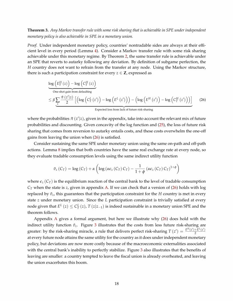
Appendix A gives a formal argument, but here we illustrate why (26) does hold with theindirect utility function vz. Figure 3 illustrates that the costs from less future risk-sharing aregreater: by the risk-sharing miracle, a rule that delivers perfect risk-sharing T (z′) = EH(z′)+EL(z′)

2

at every future node attains the same utility for the country as it does under independent monetarypolicy, but deviations are now more costly because of the macroeconomic externalities associatedwith the central bank’s inability to perfectly stabilize. Figure 3 also illustrates that the benefits ofleaving are smaller: a country tempted to leave the fiscal union is already overheated, and leavingthe union exacerbates this boom.

18

CT

log CT − α1+φ

vz(CT)

Figure 3: Costs and benefits of participating in fiscal union under alternative monetary regimes

3.2 An example of powerful improvement

We now show that the risk-sharing incentives can improved so much under monetary union as totransport countries from autarky to first-best.

Theorem 4. There exists a combination of parameters and endowment processes such that autarky is theonly feasible risk-sharing outcome when countries run an independent monetary policy, but a SPE with fullrisk-sharing is possible under monetary union.

Proof. We consider the simplest possible example of our framework: the symmetric iid case withunion-wide tradable output equal to 1. In the notation above, the Markov chain is reduced toa point z = 1 in every period, EH = e and EL = 1− e, with e > 1

2 . In this context, a Markovtransfer is a value T, such that

(CL

T, CHT)= (1− e + T, e− T). We consider transfers that improve

risk-sharing, in other words T ∈[0, 1

2 − e].

Appendix A demonstrates formally the following propositions. Under independent monetarypolicy, our setup collapses to a simple limited commitment model. Some risk sharing (T > 0)is feasible if the country currently in the high state is patient enough to value the benefits fromfuture reciprocity: its discount factor must be above a lower bound, βindep = 2 (1− e). Conversely,a deviation from first-best risk sharing, where T = 1

2 − e, is valuable if its discount factor is below

an upper bound βindep

, derived from the participation constraint of the country with endowmente.

Consider now the case of a monetary union, and assume countries are achieving perfect risk-sharing T = 1

2 − e. Due to the risk-sharing miracle (theorem 1), their nontradables side is perfectlystabilized, so their values from the transfer arrangement are identical to those under indepen-dent monetary policy. However, a deviation now entails an additional cost c (α, φ, e) coming from

19

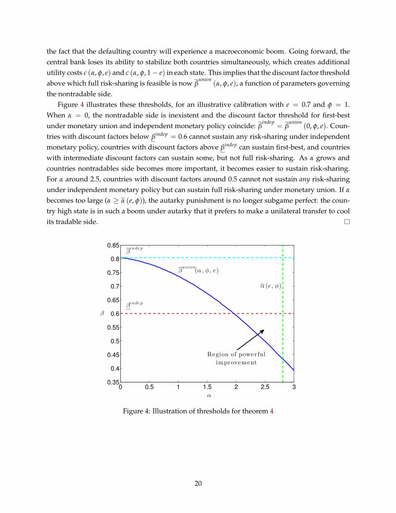
the fact that the defaulting country will experience a macroeconomic boom. Going forward, thecentral bank loses its ability to stabilize both countries simultaneously, which creates additionalutility costs c (α, φ, e) and c (α, φ, 1− e) in each state. This implies that the discount factor thresholdabove which full risk-sharing is feasible is now β

union(α, φ, e), a function of parameters governing

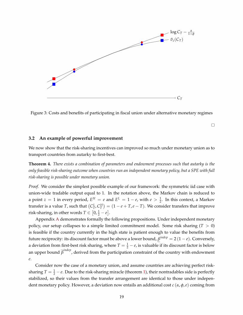
the nontradable side.Figure 4 illustrates these thresholds, for an illustrative calibration with e = 0.7 and φ = 1.

When α = 0, the nontradable side is inexistent and the discount factor threshold for first-bestunder monetary union and independent monetary policy coincide: β

indep= β

union(0, φ, e). Coun-

tries with discount factors below βindep = 0.6 cannot sustain any risk-sharing under independentmonetary policy, countries with discount factors above βindep can sustain first-best, and countrieswith intermediate discount factors can sustain some, but not full risk-sharing. As α grows andcountries nontradables side becomes more important, it becomes easier to sustain risk-sharing.For α around 2.5, countries with discount factors around 0.5 cannot not sustain any risk-sharingunder independent monetary policy but can sustain full risk-sharing under monetary union. If α

becomes too large (α ≥ α (e, φ)), the autarky punishment is no longer subgame perfect: the coun-try high state is in such a boom under autarky that it prefers to make a unilateral transfer to coolits tradable side.

0 0.5 1 1.5 2 2.5 30.35

0.4

0.45

0.5

0.55

0.6

0.65

0.7

0.75

0.8

0.85

α

β

βinde p

βinde p

βunion

(α , φ , e)

α (e, φ)

Region of powerful

improvement

Figure 4: Illustration of thresholds for theorem 4

20

3.3 Discussion

The theorems in this section are two facets of our claim that monetary union begets fiscal union.By specializing the framework of Section 2 to a case where endowments and transfer rules havelimited history dependence, we are able to prove in theorem 3 that fiscal union can improve risksharing in a particularly clear sense: any transfer rule that was feasible under independent mone-tary policy is still feasible under monetary union. And theorem 4 shows that it is possible to findpowerful improvements in this class of equilibria. We now discuss the generality of these results,by considering what would happen if we relaxed some of the assumptions imposed.

Consider relaxing the assumptions on symmetry of endowments and transfer rules. The mod-ern literature on limited commitment (Kocherlakota (1996), Alvarez and Jermann (2000), Ligonet al. (2002)) emphasizes that it is in general possible to sustain subgame-perfect outcomes thatimprove upon Markov transfer rules. In the equilibria characterized by this literature, the amounta country owes depends not only on its current and previous state, but on the full history of pastshocks, which an endogenous state variable (promised utility) keeps track of. For this more gen-eral class of equilibria, theorem 3 is in general no longer true. In particular, the country hitting itsparticipation constraint is no longer unambiguously the country which would experience a boomif if left the union: a country with a history of very bad shocks may be held at its participationconstraint as it is called upon to pay back in a mild state, even if its endowment is still relativelylow. However, even under this class of equilibria, there is still a sense in which risk-sharing isameliorated under monetary union: the discount factor thresholds to attain first-best are orderedβ

union ≤ βindep

. In fact, it is generally possible to find powerful improvements as in theorem 4for these more general endowment structures. Because of the risk-sharing miracle, the optimalpolicies in the fiscal union involve first-best risk sharing, which is simple to characterize.

Another way to relax assumptions is to add shocks to the nontradable side of the economy.Such shocks can be modelled in our framework by assuming that preferences for nontradablesare dependent on the exogenous state: αi (s). In this case, the risk-sharing miracle is in generalno longer true, as can be seen by the following argument. Assume that countries share risksto tradables perfectly, so that their relative tradables consumption is constant across all states.Since under monetary union they share the same nominal exchange rate, their relative nontradableconsumption in a state s is then, from households’ first-order condition,

C1NT (s)

C2NT (s)

= λα1 (s)α2 (s)

(27)

where λ is a constant reflecting the risk-sharing rule and nontradable prices that are constantacross all states. Unless α1 and α2 vary proportionally across states, (27) is incompatible withefficient consumption of nontradables, which still requires that C1

NT (s) = C2NT (s) = 1 (Lemma 8).

The constrained-efficient outcome that takes into account nominal rigidities, which fiscal unionwould reach absent the limited commitment constraint, does not feature perfect stabilization ineach country (Farhi and Werning (2013)). This means that joining a monetary union necessarily

21

entails some welfare losses from imperfect stabilization, but even in this case, there is still a forcepushing for welfare gains from improved incentives to share risks, so the overall welfare benefitfrom transiting into monetary union might be positive. In this sense the overall message of themodel — the risk-sharing benefits of monetary union have to be balanced against the stabilizationcosts — is unchanged by the presence of shocks to nontradables.

4 Optimal joint monetary and fiscal policy in the union

4.1 Alternative timing and the role of monetary policy

In Sections 2 and 3, we assumed that the central bank sets the exchange rate after countries an-nounced their transfers. With static welfare maximization as its objective, the central bank waslimited to stabilizing the aggregate economy ex post, without any commitment power or abilityto internalize the sustainability of fiscal union. This assumption allowed us to evaluate the directeffects of monetary union, without considering the central bank as a strategic actor in its ownright—which is inevitably a more speculative exercise.

In this section, we broaden the role of monetary policy, allowing the central bank in a monetaryunion to commit to an exchange rate policy at the beginning of each period, while retaining itsobjective of within-period welfare maximization. We now replace the timing from Figure 2 withthat depicted in Figure 5:

(ht−1)

Monetary policysets {E(s)}

Producers set PiNT

st realized

Governmentsset transfers T1, T2

End-of-periodequilibrium

(ht)

Figure 5: Alternative Timing

The choice of a state-contingent {E(s)} at the beginning of the period is driven by expectedwelfare maximization

E(s) = arg max{E(s)}

∑s

π(s)(

12

v1({ϕ1}, s, {T1(s), T2(s)}, E(s))

+12

v2({ϕ2}, s, {T1(s), T2(s)}, E(s)))

(28)

where the dependence of price distributions {ϕi} and transfers Ti(s) on monetary policy (throughthe reaction functions of nontradable pricesetters and governments) in (28) is left implicit.

Since the central bank moves first, it can internalize the effect of its decision on governments’incentives to make transfers, and it will not necessarily find aggregate stabilization optimal—thus overturning the result from Lemma 4. It may instead devise policy that actively encourages

22

sustained fiscal union, expanding upon the complementarity between monetary and fiscal unionderived in Section 3.

4.2 Expansionary monetary policy and aggregate dispersion

To illustrate the role of monetary policy in this new environment, we specialize Assumption 5 toa simpler case where the stochastic process for endowments is iid across periods, and symmetricwithin each period.

Assumption 6. There exist finitely many z ∈ Z, each of which is associated with a probability π(z) and apair of endowment levels EH(z) ≥ EL(z). Endowments are iid across periods, and in each period are drawnsuch that for each z,

Pr(

E1 = EH (z) and E2 = EL(z))= Pr

(E1 = EL (z) and E2 = EH(z)

)=

12

π(z)

We will characterize the optimal relationship between the stance of monetary policy and thedistribution of endowments across states. As in Section 3, we consider equilibria with symmetricstrategies that depend only on the current state (and whether there has yet been a deviation),rather than depending on the full history of past actions. We also repeat Assumption 3 by rulingout extreme cases where the boom in a country is so great that a unilateral transfer is worthwhile.

Assumption 7. Consider equilibria where the government receiving endowment H makes transfer T(z; d),where z ∈ Z is the aggregate state and d ∈ {0, 1} is an indicator specifying whether play is on or off theequilibrium path. Also restrict attention to equilibria where unilateral transfers are never worthwhile.

Observe that the restriction on strategies in Assumption 7, along with the symmetry of theendowment process, ensures, just as in Lemma 8, that price-setters in both countries set the samenontradable price. We can again normalize this price to 1: P1

NT = P2NT ≡ 1.

Now suppose that, out of all the equilibria consistent with Assumption 7, we aim to character-ize the equilibrium with the highest expected welfare. Quantities in this equilibrium must solvethe following planning problem:

max ∑z

π(z)(

w(EHT (z)− T(z), p(z)) + w(EL

T(z) + T(z), p(z)))

(29)

s.t. w(EHT (z), p(z))− w(EH

T (z)− T(z), p(z)) ≤ V ∀z (30)

∑z

π(z) · τH(z) + τL(z)2

= 0 (31)

where p(z) ≡ PT(z)/PNT = 1 is the relative price of tradables and nontradables in state z,w(CT, p) ≡ log CT + α

(log(αpCT)− (αpCT)

1+φ

1+φ

)is the indirect utility function corresponding to

CT, and V is the difference between expected future welfare along the equilibrium path and ex-pected future welfare following a deviation. (30) is simply the participation constraint, which isnecessary to ensure that the government with the high endowment makes transfer T(z) rather

23

than deviating and hoarding its entire endowment; while (31) is imposed by nontradable price-setting, following (20) in Lemma 5.

In the previous environment, Lemma 4 showed that the central bank stabilizes the aggregateeconomy of the monetary union, setting the average labor wedge across both countries to zero.More generally, the average labor wedge summarizes the nontradable side of the union econ-omy: a negative labor wedge corresponds to an aggregate boom, while a positive labor wedgecorresponds to an aggregate bust. In an optimum equilibrium that solves the planning problem(29)-(31), the central bank no longer seeks stabilization in every state. Instead, there is a remark-ably simple relationship between macroeconomic conditions and dispersion EH(z)/EL(z) of theendowments, captured in the following theorem.

Theorem 5. Consider the endowment process given by Assumption 6 and equilibria as described by As-sumption 7. In the subgame perfect equilibrium with maximal expected welfare, (τH(z) + τL(z))/2is weakly decreasing in the dispersion EH(z)/EL(z) between endowments. It is strictly decreasing inEH(z)/EL(z) for any z such that risk-sharing is neither perfect (CH

T (z) = CLT(z)) nor absent (CH

T (z) =

EH(z)).

In other words, in the optimal equilibrium, the central bank creates booms when dispersion ishigh. The intuition for this result is simple: when endowments are more dispersed, risk sharing ismore important, and the country with a high endowment will be more willing to make a transferwhen it is experiencing more of a boom. The central bank is willing to accept the cost of a partlyoverheated union-wide economy in order to create this boom and facilitate risk sharing in thefiscal union.

More concretely, consider the participation constraint (30), with the indirect utility function wexpanded:

(1 + α)(

log(EHT (z))− log(EH

T (z)− T(z)))

− α

1 + φα1+φ p(z)1+φ

(EH

T (z)1+φ − (EHT (z)− T(z))1+φ

)≤ V (32)

Given the stipulation in Assumption 7 that unilateral transfers are not optimal, the left side of (32)must be increasing in T(z); when the transfer is larger, making a transfer is less desirable relativeto autarky. Since higher p(z) decreases the total value on the left and relaxes the constraint, itenables higher transfers. Hence when transfers are particularly valuable—as in cases of highdispersion—it is worthwhile to raise p(z) to the point where there is an aggregate boom, tradingoff the (initially) second-order costs of aggregate overexpansion against the first-order benefits ofbetter risk sharing.

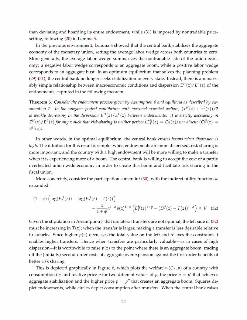
This is depicted graphically in Figure 6, which plots the welfare w(CT, p) of a country withconsumption CT and relative price p for two different values of p, the price p = p′ that achievesaggregate stabilization and the higher price p = p′′ that creates an aggregate boom. Squares de-pict endowments, while circles depict consumption after transfers. When the central bank raises

24

the relative price from p′ to p′′, at high levels of consumption there is even more of a boom, at-tenuating the within-period welfare loss from making a transfer and leaving the high-endowmentcountry’s participation constraint easier to satisfy. The change in monetary policy causes a first-order decrease in welfare for the booming high-endowment country and a first-order increase inwelfare for the depressed low-endowment country, netting out to only a second-order loss for theunion as a whole when p′′ is close to the stabilization level p′. At the margin, this loss is offset bythe benefits from easing the participation constraint.

CT

w(CT, p′′)w(CT, p′)

Figure 6: Welfare and transfer incentives under different monetary policies

The logic of Figure 6 suggests that the central bank should create a boom whenever the par-ticipation constraint is binding—which will generally be the case when perfect risk sharing is notachieved. Of course, it is not possible for the central bank to create a boom in every state: thenontradable sector sets prices that achieve aggregate stabilization in expectation, as indicated by(31). The central bank can only shape the relative pattern of boom and bust across states, not cre-ate booms across the board—and, as Theorem 5 finds, in the best equilibrium it chooses to createbooms in states with more dispersed endowments, when it is particularly important to loosenparticipation constraints and encourage transfers.

5 Conclusion

In this paper, we have examined how monetary union facilitates the formation of a stronger fiscalunion. We have seen, in an important special case, how any risk-sharing arrangement that can besustained under independent monetary policy can also be sustained under monetary union. Infact, dramatic improvement is possible: even when no risk-sharing is possible in equilibrium withindependent policy, monetary union can sometimes bring governments to a first-best outcome.

25

The key force is the complementarity of monetary and fiscal union: when countries moreeffectively share risks, their outcomes are more closely aligned, and a central bank that stabilizesthe union-wide economy can come closer to stabilizing each individual economy as well. This notonly makes fiscal union a desirable counterpart to monetary union—as is widely understood—butalso provides a channel through which monetary integration can enable otherwise unsustainablerisk-sharing. Without independent monetary policy as a fallback, governments have a greaterstake in preserving joint fiscal arrangements. This bears out the progression from monetary tofiscal union envisaged in the literature on sequencing theory; and it suggests a possible upside toa common currency, when most models featuring nominal rigidities offer only drawbacks.

Further exploring the role of monetary policy in a fiscal union, we found that when a union-wide central bank behaves strategically—taking the sustainability of the fiscal union into account—the optimal rule is expansionary when dispersion within the monetary union is high. Booms makegovernments more willing to provide transfers, and these transfers are most important when out-comes vary greatly within the union. A singleminded emphasis on stabilization is not optimal.

To what extent are the forces in this paper visible in practice? Certainly the Euro Area todayis far from perfect risk sharing—the willingness of the core to subsidize the periphery has clearlimits. At the same time, the level of cross-country support under monetary union, although oftenfrustratingly limited, has greatly exceeded what came before. There have been multiple bailoutsand transfer schemes—both explicit and implicit, often taking the form of below-market lending—made with the explicit intent of preserving the common currency’s viability.

Our model offers other reasons for guarded optimism. Although we show in Theorem 3 thatmonetary union expands the set of attainable risk sharing equilibria, we cannot be sure that gov-ernments will immediately take advantage of this feature by coordinating on the better equilibria.(After all, autarky is always an equilibrium as well.) But as participants become aware of theheightened importance of fiscal union when exchange rates are no longer free to adjust, they maylearn to play the equilibrium with improved risk sharing.

Monetary policy also has an important role. In recent years, dispersion in Euro Area outcomeshas coincided with the deepest aggregate slump in decades. This is exactly the opposite of theoptimal arrangement in Theorem 5, which prescribes monetary accommodation that creates aboom whenever members’ fates diverge and the fiscal union is under stress. To some extent,this inconsistency may be due to limitations on monetary policy that this model leaves out—inparticular, the zero lower bound. But the insufficiently expansionary policy in the Euro Areais also partly by choice: the ECB raised rates in 2011, just as the fiscal prospects of peripheralcountries were rapidly deteriorating, and it has since been hesitant to employ unconventionalexpansionary policy. Our model implies that for the full promise of fiscal union to be realized,very different choices are needed from monetary policymakers.

Monetary union begets fiscal union—but not necessarily overnight.

26

References

Abreu, Dilip, “On the Theory of Infinitely Repeated Games with Discounting,” Econometrica,March 1988, 56 (2), 383–396.

Allard, Céline, Petya Koeva Brooks, John C. Bluedorn, Fabian Bornhorst, Katharine M. Christo-pherson, Franziska Ohnsorge, Tigran Poghosyan, and IMF Staff Team, “Toward a FiscalUnion for the Euro Area,” IMF Staff Discussion Note, September 2013, 13/09.

Alvarez, Fernando and Urban J. Jermann, “Efficiency, Equilibrium, and Asset Pricing with Riskof Default,” Econometrica, July 2000, 68 (4), 775–797.

Balassa, Béla, The Theory of Economic Integration, 1st ed., Routledge, 1962.

Baldwin, Richard, “Sequencing Asian Regionalism: Theory and Lessons from Europe,” Journal ofEconomic Integration, March 2012, 27 (1), 1–32.

and Charles Wyplosz, Economics Of European Integration, 4th revised edition edition ed.,McGraw-Hill Higher Education, April 2012.

Barro, Robert J. and David B. Gordon, “Rules, Discretion and Reputation in a Model of MonetaryPolicy,” Journal of Monetary Economics, 1983, 12 (1), 101–121.

Benigno, Pierpaolo, “Optimal Monetary Policy in a Currency Area,” Journal of International Eco-nomics, July 2004, 63 (2), 293–320.

Chari, V.V., Allessandro Dovis, and Patrick J. Kehoe, “Rethinking Optimal Currency Areas,”Manuscript, September 2013.

Clarida, Richard, Jordi Galí, and Mark Gertler, “The Science of Monetary Policy: A New Keyne-sian Perspective,” Journal of Economic Literature, December 1999, 37 (4), 1661–1707.

Coate, Stephen and Martin Ravallion, “Reciprocity Without Commitment: Characterization andPerformance of Informal Insurance Arrangements,” Journal of Development Economics, February1993, 40 (1), 1–24.

Estevadeordal, Antoni and Kati Suominen, “Sequencing Regional Trade Integration and Coop-eration Agreements,” World Economy, January 2008, 31 (1), 112–140.

Farhi, Emmanuel and Iván Werning, “Fiscal Unions,” manuscript, March 2013.

Friedman, Milton, “The Case for Flexible Exchange Rates,” in “Essays in Positive Economics,”University of Chicago Press, 1953.

Fuchs, William and Francesco Lippi, “Monetary Union with Voluntary Participation,” The Reviewof Economic Studies, April 2006, 73 (2), 437–457.

27

Galí, Jordi and Tommaso Monacelli, “Monetary Policy and Exchange Rate Volatility in a SmallOpen Economy,” The Review of Economic Studies, July 2005, 72 (3), 707–734.

and , “Optimal Monetary and Fiscal Policy in a Currency Union,” Journal of InternationalEconomics, September 2008, 76 (1), 116–132.

Gustavsson, Sverker, “Monetary Union without Fiscal Union: A Politically Sustainable Asymme-try?,” in “EMU: Economic and Political Implications” Pittsburg, PA June 1999.

Haas, Ernst B., The Uniting of Europe: Political, Social, and Economic Forces, Stanford UniversityPress, 1958.

Kehoe, Timothy J. and David K. Levine, “Debt-Constrained Asset Markets,” The Review of Eco-nomic Studies, October 1993, 60 (4), 865–888.

Kenen, Peter, “The Theory of Optimum Currency Areas: An Eclectic View,” in Robert A. Mundelland A. K. Swoboda, eds., Monetary Problems of the International Economy, Chicago UniversityPress, 1969.

Kocherlakota, Narayana R., “Implications of Efficient Risk Sharing without Commitment,” TheReview of Economic Studies, October 1996, 63 (4), 595 –609.

Ligon, Ethan, Jonathan P. Thomas, and Tim Worrall, “Informal Insurance Arrangements withLimited Commitment: Theory and Evidence from Village Economies,” The Review of EconomicStudies, January 2002, 69 (1), 209–244.

McKinnon, Ronald I., “Optimum Currency Areas,” The American Economic Review, September1963, 53 (4), 717–725.

Mundell, Robert A., “A Theory of Optimum Currency Areas,” The American Economic Review,September 1961, 51 (4), 657–665.

A Appendix: proofs of theorems

Proof of Lemma 1. Substituting production into preferences

log (CT) + α

ε

ε− 1log(∫

j

(Cj

NT

) ε−1ε dj

)−

(∫j Cj

NTdj)1+φ

1 + φ

and taking a first-order condition with respect to Ck

NT shows that

(Ck

NT)− 1

ε∫j

(Cj

NT

) ε−1ε dj

=

(∫jCj

NTdj)φ

∀k

28

This shows that the efficient allocation is constant consumption across goods, CkNT = C∗NT ∀k, and

further that CNT satisfies1

CNT= Cφ

NT ⇒ C∗NT = 1

Proof of Lemma 4. Define the function CiNT (e) = α e

PiNT

CiT, and note that dCi

NT(e)de = α

CiT

PiNT

=Ci

NT(e)e .

Under independent monetary policy, the central bank chooses the exchange rate e to maximize

vi (e) = log(

CiT

)+ α

(log(

CiNT (e)

)−(∆i

NTCiNT (e)

)1+φ

1 + φ

)

Its first order condition is

αCi

NT (e)e

(1

CiNT (e)

−(

∆iNT

)1+φ (Ci

NT (e))φ)

= 0

resulting in

1−(

∆iNTCi

NT

)1+φ= 0

combining the definition of the labor wedge in (16) with labor market clearing (11), we obtain

τi = 1− CiNT∆i

NT

(Ni)φ

= 1−(

CiNT∆i

NT

)1+φ= 0

The central bank’s exchange rate choice E i ≡ e is given by

E i =1α

PiNT

∆iNTCi

T(33)

Under joint monetary policy, the central bank chooses e to maximize

12

v1 (e) +12

v2 (e)

resulting in the first-order condition

12

(C1

NTe

)(1

C1NT−(

∆1NT

)1+φ (C1

NT

)φ)+

12

(C1

NTe

)(1

C2NT−(∆2

NT)1+φ (

C2NT)φ)

= 0

12

(1−

(∆1

NTC1NT

)1+φ)+

12

(1−

(∆2

NTC2NT)1+φ

)= 0

12

τ1 +12

τ2 = 0

29

which is equation (18). That is, the central bank’s exchange rate choice E solves

12

(∆1

NTαE

P1NT

C1T

)1+φ

+12

(∆2

NTαE

P2NT

C2T

)1+φ

= 1 (34)

resulting in

E =1α

(12

(P1

NT

∆1NTC1

T

)−(1+φ)

+12

(P2

NT∆2

NTC2T

)−(1+φ))− 1

1+φ

(35)

Proof of Lemma 5. Using the relationship between consumer nontradable and tradable demand (4),we can rewrite firm profits (7) given price p, when the nominal wage is W i (s), the nominal ex-change rate is E i (s), and the price index for nontradables is Pi

NT (s), as

ψi,j (p) =(

p−(

1 + τiL

)W i (s)

)( pPi

NT (s)

)−ε

αE i (s)

PiNT (s)

CiT (s) (36)

Firms maximize the expected level of (36), valuing nominal profits in each state using the nominalstochastic discount factor 1

E i(s)CiT(s)

:

Π (p) = ∑s

π (s|s−1)1

E i (s)CiT (s)

(p−

(1 + τi

L

)W i (s)

)( pPi

NT (s)

)−ε

αE i (s)

PiNT (s)

CiT (s)

= α ∑s

π (s|s−1)(

p−(

1 + τiL

)W i (s)

)( pPi

NT (s)

)−ε1

PiNT (s)

The first-order condition yields

PijNT =

(1 + τi

L

) ε

ε− 1

∑s π (s|s−1)(

1Pi

NT(s)

)1−εW i (s)

∑s π (s|s−1)(

1Pi

NT(s)

)1−ε(37)

Hence, all firms set the same price Pi,jNT = Pi

NT = PiNT (s) ∀s, and (37) simplifies to

PiNT =

(1 + τi

L

) ε

ε− 1 ∑s

π (s|s−1)W i (s) (38)

From the household labor supply condition (6) we know that

W i (s)Pi

NT= Ci

NT (s)(

Ni (s))φ

= 1− τi (s)

30

where the latter equality holds because price dispersion is4iNT (s) = 1 in all states. We obtain

∑s

π (s|s−1) τi (s) = 1− 1− 1ε

1 + τiL

Since in each country the labor subsidy is set at the level τiL = − 1

ε , equation (20) obtains. Notethat if the subsidy is set at any level τi

L > − 1ε , the optimal price-setting problem is to equalize

the expected labor wedge to a strictly positive number, a condition inconsistent with the centralbank’s exchange-rate setting policy.

To understand the logic behind the equilibrium determination of relative prices, we furthercharacterize the price level consistent with a given expectation of the central banks’ exchange ratepolicy

{E i (s)

}. Using market clearing (11) with 4i

NT (s) = 1, we obtain Wi(s)Pi

NT=(Ci

NT (s))1+φ.

Using (4) and (9) into equation (38), we then find

(1 + τL)ε

ε− 1

(∑

sπ (s|s−1)Ci

NT (s)1+φ

)= (1 + τL)

ε

ε− 1

∑s

π (s|s−1)

(αE i (s)Ci

T (s)Pi

NT

)1+φ = 1

and results in an equilibrium price level of

PiNT =

((1 + τL)

ε

ε− 1

) 11+φ

α

(∑s∈S

π (s|s−1)(E i (s)Ci

T (s))1+φ

) 11+φ

(39)

When τiL > − 1

ε , monopolists collectively target a price that is higher than an average of E i (s)CiT (s).

This is inconsistent with central bank optimality. For example, under independent monetary pol-icy, the central bank’s exchange rate decision (33) leads to E i (s)Ci

T (s) = 1α Pi

NT in every state, andit is easy to see that these equations do not have a fixed point with positive prices.

Proof of Lemma 6. Suppressing the dependence on st−1, the central bank’s exchange rate choice (35)in the absence of price dispersion is

E (s) = 1α

(12

(P1

NT

C1T (s)

)−(1+φ)

+12

(P2

NTC2

T (s)

)−(1+φ))− 1

1+φ

(40)

while the monopolists’ price setting conditions under the labor subsidy τ1L = τ2

L = − 1ε lead to

nontradable prices given by (39)

P1NT = α

(∑s∈S

π (s|s−1)(E (s)C1

T (s))1+φ

) 11+φ

(41)

P2NT = α

(∑s∈S

π (s|s−1)(E (s)C2

T (s))1+φ

) 11+φ

(42)

31

Define ρ ≡ P2NT

P1NT

as the relative price of nontradables in the two countries. Exploiting the homo-geneity of equations, using (40) we obtain that

E (s)P1

NT=

1α

(12

(1

C1T (s)

)−(1+φ)

+12

(ρ

C2T (s)

)−(1+φ))− 1

1+φ

(43)

and this allows to rewrite (41) as

1 = α

(∑s∈S

π (s|s−1)

(E (s)P1

NTC1

T (s))1+φ

) 11+φ

=

∑s∈S

π (s|s−1)

(12+

12

(ρC1

T (s)C2

T (s)

)−(1+φ))−1

11+φ

The relative price ρ is therefore a solution to

∑s∈S

π (s|s−1)

(12+

12

(C2

T (s)ρC1

T (s)

)(1+φ))−1

= 1 (44)

The function ρ→ ∑s∈S π (s|s−1)

(12 +

12

(C2

T(s)ρC1

T(s)

)(1+φ))−1

is strictly increasing in ρ, with limits

12 as ρ → 0 and 2 as ρ → ∞, so (44) has a unique solution. Equation (44) then delivers a uniquesolution for all relative prices E(s)P1

NT, s ∈ S, and therefore for E(s)P2

NT= E(s)

P1NT

1ρ , s ∈ S also. These relative

prices are consistent with (42) because satisfaction of (44) ensures that

0 = ∑s∈S

π (s|s−1)

12 − 1

2

(C2

T(s)ρC1

T(s)

)(1+φ)

12 +

12

(C2

T(s)ρC1

T(s)

)(1+φ)

= ∑s∈S

π (s|s−1)

12

(ρC1

T(s)C2

T(s)

)(1+φ)− 1

2

12

(ρC1

T(s)C2

T(s)

)(1+φ)+ 1

2

= ∑s∈S

π (s|s−1)

1− 1

12

(ρC1

T(s)C2

T(s)

)(1+φ)+ 1

2

so we also have

∑s∈S

π (s|s−1)

(12+

12

(ρC1

T (s)C2

T (s)

)(1+φ))−1

= 1

This result is another illustration of the redundancy of equations: using τi (s) to denote the la-bor wedge in country i and state s, price-setting in country 1 implies ∑ π (s|s−1) τ1 (s) = 0, and

32

monetary policy implies τ1 (s) + τ2 (s) = 0 for all s, from we obtain ∑ π (s|s−1) τ2 (s) = 0.

Another proof of theorem 1. Following the proof of Lemma 6, consider the special case where trans-fers ensure full risk-sharing ( C2

T(s)C1

T(s)= λ for all states s). The unique solution to (44) is then clearly

ρ = λ. In this case E(s)P1NT

= 1αC1

T(s), E(s)P2

NT= 1

αC2T(s)

, and nontradables are at their efficient level in bothcountries and in all states. This is the risk-sharing miracle.

Sufficient conditions for assumption 3. Consider the period indirect utility function attained by coun-try i when choosing to make transfer T, taking as given the transfer T−i made by the other countryas well as the equilibrium reaction of the central bank to

{T, T−i}, which we denote E (T) to make

the dependence of the exchange rate on the transfer explicit. Denote CiT (T) = Ei

T + T−i − T andCi

NT (T) = αE(T)Pi

NTCi

T (T). Note that

dCiNT (T)dT

= α1

PiNT

(E ′ (T)Ci

T (T)− E (T))

= −αE (T)Pi

NT

(1− E

′ (T)E (T) Ci

T (T))

= −CiNT (T)

CiT (T)

(1− E

′ (T)E (T) Ci

T (T))

In a Nash equilibrium where current fiscal policy only has impact on current utility, T is chosen tomaximize

vi (T) = log(

CiT (T)

)+ α

(log(

CiNT (T)

)−(Ci

NT (T))1+φ

1 + φ

)The first-order condition of this problem is

dvi (T)dT

= − 1Ci

T (T)− α

CiNT (T)

CiT (T)

(1− E

′ (T)E (T) Ci

T (T))(

1Ci

NT (T)− Ci

NT (T)φ

)

= − 1Ci

T (T)

1 + α

(1− E

′ (T)E (T) Ci

T (T))(

1− CiNT (T)1+φ

)︸ ︷︷ ︸

τi(T)

where τi (T) is country i’s labor wedge, a determined by the central bank’s reaction to

(T, T−i)

and to the prices in place. From (34), this is done to enforce

12

(αE (T)P1

NTC1

T (T))1+φ

+12

(αE (T)P2

NTC2

T (T))1+φ

= 1

33

differentiating we find

12

(αE (T)P1

NTC1

T (T))1+φ

[E ′ (T)E (T) +

C1′T (T)

C1T (T)

]+

12

(αE (T)P2

NTC2

T (T))1+φ

[E ′ (T)E (T) +

C2′T (T)

C2T (T)

]= 0

which leads to the central bank adjustment rule

E ′ (T)E (T) = −1

2

(1− τ1 (T)

) C1′T (T)

C1T (T)

− 12(1− τ2 (T)

) C2′T (T)

C2T (T)

For country i, an increase in own transfer reduces home country tradable consumption and in-creases foreign: Ci′

T (T) = −1 and C−i′T (T) = 1, so

E ′ (T)CiT (T)

E (T) =12

(1− τi (T)

)− 1

2

(1− τ−i (T)

) CiT (T)

C−iT (T)

=12

(1− τi (T)

)− 1

2

(1 + τi (T)

) CiT (T)

C−iT (T)

=12

(1− Ci

T (T)C−i

T (T)

)− 1

2τi (T)

(1 +

CiT (T)

C−iT (T)

)

and finally

1− E′ (T)Ci

T (T)E (T) =

12

(1 +

CiT (T)

C−iT (T)

)(1 + τi (T)

)an expression which is always strictly positive, given that τi (T) > −1. We therefore have

dvi (T)dT

= − 1Ci

T (T)

[1 + α

12

(1 +

CiT (T)

C−iT (T)

)(1 + τi (T)

)τi (T)

]

The function τ 7→ 1 + α 12

(1 + Ci

TC−i

T

)(1 + τ) τ has value 1 at both τ = 0 and τ = −1. Its minimum

1− α 18

(1 + Ci

T(T)C−i

T (T)

)is attained at τ = − 1

2 . If

α <8

1 + CiT(T)

C−iT (T)

then vi(T)dT < 0 and country i prefers not to make a transfer.

A sufficient condition for countries not to want to make transfers in autarky is then

α <8

1 + maxs

{E1

T(s)E2

T(s); E2

T(s)E1

T(s)

}

34

more generally, the condition is that 1 + α 12

(1 + Ei

T(s)

EjT(s)

) (1 + τi (s)

)τi (s) > 0 for the labor wedge

in country i and state s that results from central bank optimization given an autarkic fiscal policy,that is

τi (s) = 1− 1

12 +

12

(ρEi

T(s)

EjT(s)

)−(1+φ)

where ρ is the solution to (44).

Proof of Lemma 8. Suppose that countries have endowment processes governed by assumption 5and follow Markov transfer rules. From (44), given any z−1, the relative nontradables price ρ =P2

NT(z−1)

P1NT(z−1)

solves

∑s∈S

π (z|z−1)

12

(12+

12

(EH (z)− T (z, z−1)

ρ (EL (z) + T (z, z−1))

)(1+φ))−1

+12

(12+

12

(EL (z) + T (z, z−1)

ρ (EH (z)− T (z, z−1))

)(1+φ))−1 = 1

(45)

making use of the equality12

112 +

12 x

+12

112 +

12

1x

= 1 ∀x

applied separately to each pair x =(

EH(z)−T(z,z−1)EL(z)+T(z,z−1)

)(1+φ), we see that ρ = 1 is a solution to (45),

hence its unique solution by Lemma 6.

Proof of theorem 3. By Lemma 8, the relative nontradables price in monetary union is ρ = 1. Thisdelivers the indirect utility function

v (C) = log (C) + α

(log (αεz (C)C)− (αεz (C)C)1+φ

1 + φ

)

where the common real exchange rate for both countries is given by

εz (C) =1α

(12

(1C

)−(1+φ)

+12

(1

E (z)− C

)−(1+φ))− 1

1+φ

(46)

with E (z) = EH (z) + EL (z). This implies that

gz (C) ≡ αεz (C)C =

(12+

12

(C

E (z)− C

)−(1+φ))− 1

1+φ

(47)

is a strictly increasing function of C. gz (C) attains 1 at C = E(z)2 .

The proof of theorem (3) now follows. By definition of subgame perfection, the H country does

35

not want to refrain from the transfer at any node zt:

log(

CHT(zt))+ β ∑

zh�zt

π(zh|zt)2

(log(

CHT(zt))+ log

(CL

T(zt)))

≥ log(

EHT(zt))+ β ∑

zh�zt

π(zh|zt)2

(log(

EHT(zt))+ log

(EL

T(zt)))

Using the Markov structure, the participation constraints for all z ∈ Z can be written

log(

EHT (z)

)− log

(CH

T (z))

︸ ︷︷ ︸One-shot gain from defaulting

≤ β ∑z

π (z′|z)2

[(log(

CLT(z′))− log

(EL (z′)))− (log

(EH (z′))− log

(CH

T(z′)))]

︸ ︷︷ ︸Expected loss from lack of future risk-sharing

where π (z′|z) are the elements of the matrix Π = Πz (I − βΠz)−1, which take into account therelevant mix of future probabilities and discounting. Due to the ordering (25) and the concavityof log, we have(

log(

CLT (z)

)− log

(EL (z)

))−(

log(

EH (z))− log

(CH

T (z)))≥ 0

Consider sustaining the same SPE under monetary union using the same on-path and off-pathactions. Lemma 8 implies that both countries have the same real exchange rate at every node, sothey evaluate tradable consumption levels using the same indirect utility function

vz (C) = log (C) + α

(log (αεz (C)C)− 1

1 + φ(αεz (C)C)1+φ

)where εz (C) is given in (46). Recall from (47) that gz (C) ≡ αεz (C)C is strictly monotone andattains the value 1 (the efficient nontradables consumption level) at C = EH(z)+EL(z)

2 . This is aconsequence of the risk-sharing miracle. Since

f (x) ≡ α

(log (x)− 1

1 + φx1+φ

)is a concave function with a maximum at x = 1, the function vz (C) − log (C) = f (gz (C)) issingle-peaked with a maximum at EL(z)+EH(z)

2 . In particular

f(

gz

(EH (z)

))≤ f

(gz

(CH

T (z)))

∀z

f(

gz

(EL (z)

))≤ f

(gz

(CL

T (z)))

∀z

from which it follows that

vz

(EH (z)

)− vz

(CH

T (z))≤ log

(EH (z)

)− log

(CH

T (z))∀z

36

and thatlog(

CLT (z)

)− log

(EL (z)

)≤ vz

(CL

T (z))− vz

(EL (z)

)∀z

Combining these inequalities, we obtain

vz

(EH

T (z))− vz

(CH

T (z))≤ log

(EH

T (z))− log

(CH

T (z))

≤ β ∑z

π (z′|z)2

[(log(

CLT (z)

)− log

(EL (z)

))−(

log(

EH (z))− log

(CH

T (z)))]

≤ β ∑z

π (z′|z)2

[(vz

(CL

T (z))− vz

(EL (z)

))−(

vz

(EH (z)

)− vz

(CH

T (z)))]

which guarantees that the participation constraint for the H country is met in every state z undermonetary union, as claimed.

Proof of theorem 4. We consider the simplest possible example of our framework: the symmetriciid case with union-wide tradable output equal to 1. In the notation above, the Markov chain isreduced to a point z = 1 in every period, EH = e and EL = 1− e, with e > 1

2 . In this context, aMarkov transfer is a value T, such that

(CL

T, CHT)= (1− e + T, e− T). We consider transfers that

improve risk-sharing, in other words T ∈[0, 1

2 − e].

Under independent monetary policy, given the flow value from the nontradables side is alwaysconstant at f ∗ = f (1) ≡ − α

1+φ , the value of being in the high state under the contract is

VH (T) = log (e− T) +β

1− β

(12

log (e− T) +12

log (1− e + T))+

f ∗

1− β

The participation constraint states that VH (T) ≥ VH (0). Since VH is concave in T, there exists aT > 0 such that this constraint is satisfied if, and only if

dVH

dT

⌋T=0

= −1e+

β

1− β

12

(−1

e+

11− e

)≥ 0

that is, if and only ifβ ≥ βindep = 2 (1− e)

Suppose countries now are sharing risks perfectly T = 12 − e, therefore obtaining

(CL

T, CHT)=( 1

2 , 12

)and value

VFB =1

1− β

(log(

12

)+ f ∗

)Consider the deviation of the country in the high state, which is punished by the grim triggerstrategy. This deviation is valuable if

log (e)− log(

12

)︸ ︷︷ ︸

One-shot gain from defaulting

≥ β

1− β

12

(2 log

12− log (e)− log (1− e)

)︸ ︷︷ ︸

Expected loss from lack of future risk-sharing

37

Which is equivalent to the condition

β ≤ βindep

= 2log (e)− log

( 12

)log (e)− log (1− e)

≤ 1

Consider now the case of a monetary union, and assume countries are achieving perfect risk-sharing T = 1

2 − e. Due to the risk-sharing miracle (theorem 1), their nontradables side is perfectlystabilized and they obtain VFB. However, a deviation now entails the additional cost

c (e) = f ∗ − f (g (e)) = f (1)− f (g (e)) = α

(g (e)1+φ − 1

1 + φ− log (g (e))

)≥ 0

where nontradable consumption, considering the central bank reaction, is

g (e) =

(12+

12

(e

1− e

)−(1+φ))− 1

1+φ

> 1

for the country in the H state and and g (1− e) < 1 for the country in the L state. The conditionfor a profitable deviation is now

log (e)− log(

12

)− c (e) ≥ β

1− β

12

(2 log

12− log (e)− log (1− e) + c (e) + c (1− e)

)which shows clearly that monetary union both lowers the benefit and raises the costs of defaulting.A country therefore finds it profitable to deviate from first-best risk-sharing under monetary unionwhen

β ≤ βunion

(α, φ, e) = 2log (e)− log

( 12

)− c (e)

log (e)− log (1− e) + c (1− e)− c (e)

It is simple to show that βunion

(α, φ, e) is strictly decreasing in α with limα→∞ βunion

(α, φ, e) < 0.This has two consequences. First,

βunion

(α, φ, e) ≤ βunion

(0, φ, e) = βindep

formalizing our claim that first-best risk-sharing is easier to sustain under monetary union thanunder independent monetary policy. Second, there always exists values of (α, φ, e) such thatβ

union(α, φ, e) ≤ βindep. To complete the claim that countries with discount factors β

union(α, φ, e) ≤

β ≤ βindep can only sustain autarky under independent monetary policy, but can sustain full risk-sharing under monetary union, one also needs to check that autarky under monetary union isindeed subgame perfect at those parameters. This is ensured by the condition

1e+

α

g (e)

(1− (g (e))1+φ

)g′ (e) ≥ 0

38

or equivalently

α ≤ α (e, φ) =1

( e1−e )

−(1+φ)

1+( e1−e )

−(1+φ)

(g(e))1+φ−11−e

39