Monetary Sovereignty, Exchange Rates, and Capital Controls ... · MONETARY SOVEREIGNTY,EXCHANGE...
34
Monetary Sovereignty, Exchange Rates, and Capital Controls: The Trilemma in the Interwar Period MAURICE OBSTFELD, JAY C. SHAMBAUGH, and ALAN M. TAYLOR * The interwar period was marked by the end of the classical gold standard regime and new levels of macroeconomic disorder in the world economy. The interwar disorder often is linked to policies inconsistent with the constraint of the open- economy trilemma—the inability of policymakers simultaneously to pursue a fixed exchange rate, open capital markets, and autonomous monetary policy. The first two objectives were linchpins of the pre-1914 order. As increasingly democratic polities faced pressures to engage in domestic macroeconomic man- agement, however, either currency pegs or freedom of capital movements had to yield. This historical analytic narrative is compelling—with significant ramifi- cations for today’s world, if true—but empirically controversial. We apply the- ory and empirics to the interwar data and find strong support for the logic of the trilemma. Thus, an inability to pursue consistent policies in a rapidly chang- ing political and economic environment appears central to an understanding of the interwar crises, and the same constraints still apply today. [JEL F33, F41, F42, N10] 75 IMF Staff Papers Vol. 51, Special Issue © 2004 International Monetary Fund * Obstfeld is the Class of 1958 Professor of Economics at the University of California, Berkeley; a Research Associate at the National Bureau of Economic Research; and a Research Fellow at the Centre for Economic and Policy Research. He gratefully acknowledges the support of the Class of 1958 chair at Berkeley. Shambaugh is an assistant professor of economics at Dartmouth College. Taylor is a professor of economics at the University of California, Davis; a Research Associate at the National Bureau of Economic Research; and a Research Fellow at the Centre for Economic and Policy Research. He grate- fully acknowledges the support of the Chancellor’s Fellowship at the University of California, Davis. All three authors thank Julian di Giovanni and Ahmed Rahman for excellent research assistance, and are grate- ful to Robert Flood and Hélène Rey for their helpful comments.
Transcript of Monetary Sovereignty, Exchange Rates, and Capital Controls ... · MONETARY SOVEREIGNTY,EXCHANGE...
Monetary Sovereignty, Exchange Rates,and Capital Controls: The Trilemma
in the Interwar Period
MAURICE OBSTFELD, JAY C. SHAMBAUGH, and ALAN M. TAYLOR*
The interwar period was marked by the end of the classical gold standard regimeand new levels of macroeconomic disorder in the world economy. The interwardisorder often is linked to policies inconsistent with the constraint of the open-economy trilemma—the inability of policymakers simultaneously to pursue afixed exchange rate, open capital markets, and autonomous monetary policy.The first two objectives were linchpins of the pre-1914 order. As increasinglydemocratic polities faced pressures to engage in domestic macroeconomic man-agement, however, either currency pegs or freedom of capital movements had toyield. This historical analytic narrative is compelling—with significant ramifi-cations for today’s world, if true—but empirically controversial. We apply the-ory and empirics to the interwar data and find strong support for the logic ofthe trilemma. Thus, an inability to pursue consistent policies in a rapidly chang-ing political and economic environment appears central to an understanding ofthe interwar crises, and the same constraints still apply today. [JEL F33, F41,F42, N10]
75
IMF Staff PapersVol. 51, Special Issue
© 2004 International Monetary Fund
*Obstfeld is the Class of 1958 Professor of Economics at the University of California, Berkeley; aResearch Associate at the National Bureau of Economic Research; and a Research Fellow at the Centrefor Economic and Policy Research. He gratefully acknowledges the support of the Class of 1958 chair atBerkeley. Shambaugh is an assistant professor of economics at Dartmouth College. Taylor is a professorof economics at the University of California, Davis; a Research Associate at the National Bureau ofEconomic Research; and a Research Fellow at the Centre for Economic and Policy Research. He grate-fully acknowledges the support of the Chancellor’s Fellowship at the University of California, Davis. Allthree authors thank Julian di Giovanni and Ahmed Rahman for excellent research assistance, and are grate-ful to Robert Flood and Hélène Rey for their helpful comments.
In the present era of globalization, one of the most difficult challenges forgovernments—and for those who advise them—is to understand the constraints
under which policies must be designed in a world of increasing economic inter-dependence. Nowhere are these constraints more pressing than in the arena of mon-etary policy design in open economies, where the recent spate of economic crisesin developing countries, from Mexico in 1994 to East Asia in 1997 to Argentina in2001, highlighted the costs to be paid when the exchange rate regime unravels. Inthis paper we place the current quandary in a longer run context, and ask whatlessons history has for contemporary problems. Our approach brings together the-ory, empirics, and history.
The theoretical foundation of this paper casts the choices faced by policy-makers in terms of the classic macroeconomic trilemma: the idea that of the threepolicy objectives of a fixed exchange rate, open capital markets, and autonomousmonetary policy, only two can be mutually consistent and, hence, tenable as stablefeatures of the policy regime. The intuition is simple: when a country credibly andpermanently pegs its exchange rate to some base country, and when capital isfreely mobile, simple interest parity pins down the domestic interest rate, forcingit to be equal to the interest rate in the base country. We do not study what mightbe driving the intent of the authorities to manipulate nominal interest rates in theshort run, but we take as given their desire to engage in active macroeconomicmanagement over the business cycle and their belief that, due to short-run nomi-nal rigidities, such intervention might be effective.
We will also take it as given—even uncontroversial—that the defining role of asovereign monetary authority is that it will exercise such powers, when feasible anddesirable, and this will affect liquidity, and hence interest rates, at the short end ofthe market. Some deeper questions intrude, however, especially with regard to fea-sibility and desirability. On feasibility, in contrast to the stark prescriptions of thetrilemma, we know that intervention can be more continuous than dichotomous,sometimes as a result of authorities’ decisions not to peg to a fixed rate, but insteadto limit exchange rate movements to a band or “target zone.” As has been recognizedin the literature at least since the writings of Goschen (1861), this can leave somewiggle room for monetary policy—but how much? On desirability, we also have tobe careful about the intent (or objectives) of policymakers, versus their constraints(or choice set). Under some policy systems, such as the gold standard, intent was notreally a matter of debate in theory, although economic historians have noted thatsubstantial deviations were witnessed in practice (Bloomfield, 1959; and Scammell,1965). Under alternative systems, such as inflation targeting or other nominal an-chors, authorities may have varying degrees of freedom depending on the regime inplace, and depending on the regime of the partner country. Thus convergence, ordivergence, from international monetary regimes or operating rules—a function ofhistory, politics, and ideology—may lead to greater or lesser degrees of synchro-nization in policymakers’ actions.
Our approach to these difficulties is to develop a formal model as a benchmarkto guide our interpretation of the empirical findings. Using a target-zone model,one can compute the extent to which policymakers create a divergence between
Maurice Obstfeld, Jay C. Shambaugh, and Alan M. Taylor
76
short-term domestic and base-country interest rates under various policy scenar-ios. Different parameterizations allow such a model to capture both tight pegs (anarrow band) and nonpegs (an infinite band width), as well as varying degrees ofactivism on the part of policymakers as they seek to smooth out, or reinforce,monetary shocks from abroad.
The goal of the subsequent empirical work is to measure the extent to whichchanges in the relevant foreign “base” nominal interest rate pass through into the domestic nominal interest rate. The data provide some challenges. Sometimescare is needed to ensure that the correct base country is chosen, because at cer-tain times in history this choice is not necessarily obvious. Furthermore, the sta-tus of a country with respect to the fixity of its exchange rate against any basecurrency is not always clear. Another difficulty arises from the near-nonstationarityof nominal interest rates in many historical periods. That feature of the data nar-rows our choice of techniques for both time series and panel estimation. Withthese problems addressed, however, the empirical method allows us to concen-trate on the central predictions of the trilemma. To what extent do countries thatpeg and have open capital markets lose their monetary sovereignty? And do theyrecoup it when they resolve the trilemma in other ways—either by allowing theexchange rate to float, or by imposing capital controls? By dividing our sampleaccording to exchange rate regime and capital control criteria, we can examinethese questions.
The trilemma is not necessarily an easy proposition to test, but we view ourapproach as one of the more direct ways to explore its validity. Previous empir-ical tests of the trilemma have produced mixed results. Often the test has beenindirect, as with the literature on the so-called “exchange rate disconnect” (Baxterand Stockman, 1989; and Flood and Rose, 1995). These authors saw very littledifference in the statistical properties of real and nominal economic fluctuationsin fixed versus floating rate episodes, except for the volatility and comovementof real and nominal exchange rates. As a corollary it could be inferred that thetrilemma trade-offs might not impinge so tightly. Yet such an inference wouldclearly depend on additional maintained assumptions, in particular about thehorizon over which autonomy can be presumed to have an effect. Further, sincethe data used for these analyses was of low frequency, it could very well under-state the ability of monetary authorities to exert some high-frequency autonomy,even if they are subject to other constraints, such as real interest rate equality, atlonger horizons.1
A more direct approach to testing the trilemma was taken by Rose (1996) whocompared the predictions of a monetary model of exchange rates, based on moneyaggregates and outputs, with actual exchange rate movements, conditional on capi-tal controls and the exchange rate regime. His results were somewhat consistent withthe trilemma, but still weak. It could be argued that one source of weakness was theuse of the monetary model, which seems to perform poorly at higher frequencies,
MONETARY SOVEREIGNTY, EXCHANGE RATES, AND CAPITAL CONTROLS
77
1Indeed, the one “robust result” cited by Flood and Rose is a negative relationship between exchangerate and output variability (Flood and Rose, 1995, p. 18). That pattern is consistent with a role for exchangerate flexibility in dampening output fluctuations.
due to unstable money demand, and which is therefore unable to cleanly capturethe high-frequency content of the trilemma. A natural alternative is to measuremonetary policy not by a quantity, money stocks, but by a price, namely the actualinstrument used by most central banks to impose their policy—the short-terminterest rate. Ours is one of several recent studies to follow this tack (Frankel,Schmukler, and Servén, 2002; Obstfeld, Shambaugh, and Taylor, 2004; andShambaugh, 2004).
We choose to bring these theoretical and empirical tools to bear on one ofthe most turbulent periods in the history of the international macroeconomy—the interwar period. In the next section we explore the history of that period,where the narratives tell of a crisis in which the implications of the trilemmawere suddenly more apparent than ever before. Subsequent sections discuss ourtheoretical simulations, describe the data we employ, and present the empiricalresults. A concluding section sums up the lessons learned and their relevancetoday.
I. Trilemma in the Interwar Period
After introducing our footholds in theory and empirics, we now turn to historyand the interwar period, which is the object of study in this paper. The period’srelevance is clear: arguably it was in this epoch that the trilemma forcefully madeits presence felt for the first time in the great debate over the political economyof macroeconomics. For that reason, the trilemma idea resonates strongly witheconomic historians, who tend to understand the evolution of the global macro-economic order in those terms. In the interwar period, all the key ingredients ofthe trilemma came into collision (Eichengreen, 1996; and Obstfeld and Taylor,1998, 2004).
In 1913, the ideology of the classical gold standard still held sway, and inter-national capital market integration had reached its zenith, leaving the authoritieswith little room for maneuver. The rise of more democratic polities led policy-makers to seek greater autonomy than the old “rules of the game” permitted. Con-ventional wisdom argues that such a combination of inconsistent elements setthe gold standard up for its swift demise following a brief reconstruction in the1920s, a key part of the wider collapse of globalization seen during the interwaryears (Temin, 1989; and James, 2001). Some have further argued that this crisisreflected a fundamental conflict between economic globalization, or at least itsmacroeconomic manifestation in the gold standard, and the advance of democracy,a tension that would perhaps henceforth place limits on the role of markets underthe modern nation-state, although the recent so-called return to globalization hasseemingly reversed that trend (Polanyi, 1944; Yergin and Stanislaw, 1998;Lindsey, 2002; and Tortella, 2003). This is the history, therefore, not of a far-removed past but a close precursor of the present, and the same trilemma clearly hasrelevance for the choices facing policymakers today. Once again, capital markets areincreasingly fluid, an air of experimentation surrounds exchange rate regime choice,and the loss of monetary sovereignty is an issue of burning interest, especially toemerging-market countries.
Maurice Obstfeld, Jay C. Shambaugh, and Alan M. Taylor
78
Thus, the interwar period stands as a defining moment in the history of mod-ern political economy and macroeconomics, and the trilemma was the issue at thevery center of events. The historical record provides plenty of examples and anec-dotes consistent with this story. Witness the heated debate over gold resumptionat par in Britain, pitting Keynes against conventional opinion, as general laborunrest simmered in the background; or, under conditions of equal or greater socialfoment, consider the tortured compromises by French politicians in the run-up toPoincaré’s resumption at a devalued parity, and the continuing policy uncertaintyas France clung to gold until 1936. Yet, despite all of this suggestive evidence, weare unaware of any research that formally and directly tests for the presence of thetrilemma, and examines its potency, in the macroeconomic crucible of the inter-war years.
Unfortunately, this is to some degree understandable given the chaotic natureof the period. Serious empirical work of the kind we envisage requires high-frequency data collection for interest rates and clear records of the capital control andexchange rate regimes for each country. The task is daunting for the years betweenthe wars, as data can be collected only with difficulty and with substantial noise.Regime definition is often imprecise and certainly volatile. Many countries changedtheir peg and capital control status several times. Some countries were off goldbut really “shadowing” the gold standard in a desperate attempt eventually torejoin. Capital control policies varied by country in their degree of strictness. Ourown work has previously examined the trilemma empirically in the pre-1914 andpost-1945 periods, where the empirical challenges are somewhat fewer (Obstfeld,Shambaugh, and Taylor, 2004). We have since, however, constructed an interwardatabase that allows us to put the trilemma to the test at perhaps its most criticalhistorical moment.
Looking on the bright side, the extreme variation in conditions during the inter-war sample period is, of course, good news from the econometric standpoint.Whereas our previous work compared economic experiences separated by manydecades, and sometimes a century or more, the interwar period supplies all thevariation we could hope for in the space of 10 or 15 years. In that brief window,fixes and floats, controls and free markets were all tried here and there. We there-fore find ample power to identify the effects we study, although sometimes theextremely short duration of peg and float episodes makes univariate time-seriesanalysis difficult. The interwar period also follows hard on the heels of an idealbenchmark era against which we can compare our results—the classical pre-1914gold standard. Accordingly, we shall refer back to results for that period as a basisfor judging the behavior of the interwar regimes. Along the way, we also gain anopportunity to consider some related hypotheses, for example, the much-discussedswitch of the world financial center from London to New York after World War I,considered essential to the hegemony theory of an evolution from a British- to aU.S.-led world order (Kindleberger, 1986).
The central aim, however, is to test the power of the trilemma as an explanatorytool. To lay the groundwork for that test, we now turn to some important theoreticalconsiderations that help buttress our econometric approach and subsequent inter-pretations of the results.
MONETARY SOVEREIGNTY, EXCHANGE RATES, AND CAPITAL CONTROLS
79
II. Empirical Methodology and Rationale
The starting point for our econometric analysis is a panel regression of the form
(1)
where Rit is the nominal interest rate in country i on date t, Rbit is the interest ratein the “base” country, and uit is a random shock.2 Under perfect internationalcapital mobility and an exchange rate credibly pegged with a zero fluctuationband, we would expect to find ordinary least squares (OLS) estimates of β = 1and R2 = 1. In practice, however, the actual estimates differ from this hypotheti-cal benchmark case, and we wish to know if there are systematic differences in thesize of βbetween pegged exchange rate regimes and nonpegs. Our claim is that suchdivergences inform us about the scope for interest rate management, and thereforefor monetary policy independence, under alternative exchange rate regimes. As analternative way to measure the impact of a peg on the sensitivity of domestic to for-eign interest rates, we pool data from peg and nonpeg regimes and look at the mag-nitude of β2 in the regression
(2)
where PEGit takes the value 1 if country i pegs to the base currency at time t and0 otherwise.
We focus our theoretical discussion on the key slope coefficient β in equation(1), though we also consider the fit of that equation in our empirical results. A con-venient starting point for interpreting estimates of equation (1) is the generalizeduncovered interest parity relationship
(3)
where ε is the expected depreciation rate of the domestic currency (over a horizoncorresponding to that of the interest rates R and Rb) and v is a random, mean-zero,excess return or risk premium that, for convenience, we take to be exogenous.Given the model of equation (3), the OLS estimate of β in the difference regres-sion (1) satisfies
(4)
plim plim plim
1
1DIFFSˆ
, ,
βε
ρ ε σ εσ
=( )
( )= +
( )
( )
= + ( ) ( )( )
∑∑
∑
∑
∆ ∆
∆
∆ ∆
∆
∆ ∆ ∆∆
R R
RT
R
TR
RR
t btt
btt
t btt
btt
t btt
bt
. .
22
1
1
R R vb= + +ε ,
∆ ∆ ∆R R R PEG uit bit bit it it= + ×( ) +β β1 2 ,
∆ ∆R R uit bit it= +β ,
Maurice Obstfeld, Jay C. Shambaugh, and Alan M. Taylor
80
2Variants of this methodology are followed in the precursor papers by Frankel, Schmukler, and Servén(2002), Obstfeld, Shambaugh, and Taylor (2004), and Shambaugh (2004). We omit fixed effects from the pre-ceding equation on the grounds that deterministic trends in nominal interest rates are implausible; and, inpractice, when we include such fixed effects they are estimated to be indistinguishable from zero.
where ρ is a correlation coefficient, σ is a standard deviation, and T is sample size.The second term on the right-hand side of equation (4) captures the average responseof exchange rate expectations to changes in the base interest rate. Under interest par-ity, if a rise in the foreign base interest rate is accompanied by a smaller absolute risein the domestic interest—as would be the case under a system of domestic interestrate smoothing by the monetary authority—then the expected rate of currencydepreciation, ε, must simultaneously fall. This could be accomplished by allowingthe domestic currency to depreciate sufficiently in the foreign exchange market toinduce a higher expected rate of future appreciation (that is, a lower expected rate offuture depreciation). In that case, the average Σt(∆εt�∆Rbt)/T is negative for largeenough T, as is the correlation coefficient ρ(∆εt,∆Rbt), and β< 1. Alternatively, werethe home monetary authority to reinforce the effect of foreign interest shocks, onewould expect β > 1. Thus, the coefficient β measures the extent to which domesticmonetary policy has (and uses) the scope to respond to foreign interest rate shocks.
An alternative specification would be the analog of equation (1) in interestrate levels rather than differences,
(5)
Such a strategy seems inadvisable in light of the persistence of nominal interestrates in our data. For the interwar period, the monthly series of U.S. interest ratesdisplays an autocorrelation coefficient of 0.99 in monthly data, and for the vastmajority of other interest rates in our sample the presence of a unit root cannot berejected statistically.3 Thus, the assumption of a unit root in interest rates is a goodapproximation to the data.
Under a unit root, however, estimation in levels of interest rates yields
assuming the expected depreciation rate is statistically stationary. Because thestochastic trends in the interest rates dominate, levels estimates are not well suitedto yield information about interest rate independence. If international interest ratesare not cointegrated, the spurious regression problem stressed by Shambaugh(2004) can arise. In the data, we find that the residual terms in equation (1) areapproximately serially uncorrelated.
To evaluate these claims, as well as to aid in interpreting the empirical results,we perform Monte Carlo experiments using simulated data based on a formal modelof exchange rate target zones. The basic model comes from Krugman (1991) andhas been extended by Flood and Garber (1991), Froot and Obstfeld (1991),Svensson (1991), and others. To generate interest rates of noninstantaneous matu-rity, we utilize Svensson’s (1991) account of the term structure of interest rates
plim plim plimLEVELSˆ ,β
ε=
( )
( )= +
( )
( )=
∑∑
∑∑
R R
R
R
R
t btt
btt
t btt
btt
. .
2 21 1
R Rit bit it= + +α β η .
MONETARY SOVEREIGNTY, EXCHANGE RATES, AND CAPITAL CONTROLS
81
3In contrast, under the pre-1914 gold standard, nominal interest rates appear stationary. Apparent non-stationarity is the rule after World War II, as during the interwar period.
within a target zone. We compare the results of interest rate regressions under anarrow target zone (bands of ±1 percent) and a freely floating exchange rate.
It is helpful to give a brief description of the model that we use in these simu-lations.4 The time-t log exchange rate, e(t), is defined as the home price of foreigncurrency. It is determined by the forward-looking pricing equation
where x(t) is a “fundamental” economic variable driving currency value (for exam-ple, the home less the foreign money supply) and η > 0. The fundamental x followsa mean reverting process of the form
(6)
where dz is Gaussian noise.5 Under these assumptions, and an allowable (reflect-ing) fluctuation band [e,e] for the exchange rate, there is a unique price solution e = s(x), from which the expected depreciation rate of the domestic currency,
follows from Itô’s Lemma.6The preceding equation defines an instantaneous expected depreciation rate.
The interest rates available for empirical analysis apply, however, to finite matu-rities. Svensson (1991) shows that when uncovered interest rate parity holds, wecan approximate the international interest differential at maturity m by
where f (m,x) is the exchange rate expected to prevail after an interval of positivelength m has elapsed.7 We specify the base foreign interest rate Rm
b of the relevantmaturity to follow a random walk, constrained only by a lower bound of zero. In
δ m xf m x s x
m,
,,( ) = ( ) − ( )
E d
dt e
txs x s x
{ }= − ′( ) + ′′( )ξ σ2
2,
d d d ,x x t z= − +ξ σ
e t x te t
tt( ) = ( ) +
( ){ }η E d
d,
Maurice Obstfeld, Jay C. Shambaugh, and Alan M. Taylor
82
4A more detailed description of the model and methodology can be found in Obstfeld, Shambaugh,and Taylor (2004).
5In Krugman’s (1991) original model, ξ = 0. Under that assumption, however, exchange rates wouldfollow a random walk under a free float, minimizing international interest differentials. To get a bettersense for the scope for interest rate independence under a float, we therefore consider the case ξ > 0 in oursimulations, following Froot and Obstfeld (1991).
6The exchange rate solution under a free float, such that [e,e] → [−∞, + ∞], is simply:
7Of course, f (0,x) = s(x). Think of m as a fraction of a year.
ex
=+1 ηξ
.
line with equation (3), which incorporates a deviation v from interest parity, thedomestic nominal interest rate of maturity m is then modeled as
We interpret the error v as an empirical, serially uncorrelated and exogenous de-parture from the underlying economic model. Svensson (1991) shows how tosolve for the term expected depreciation rate δ(m,x). In our simulations, Rm has alower bound of zero. We further constrain the noise v to preclude pure arbitrageprofits in the target zone case (that is, we rule out interest differentials larger thanthe maximum capital loss allowed by the bands). That further constraint is neces-sary when the bands are permanent and fully credible, as we are assuming.
In practice we approximate equation (6) by a discrete-time process sampled atintervals of h = 10 minutes. The base interest rate’s level is generated as a randomwalk modified by a nonnegativity constraint. Innovations in the base interest rateand the domestic fundamentals are drawn from a bivariate normal distribution. Akey parameter in the simulated data is ρ(∆z,∆Rb), defined as the instantaneous cor-relation between the innovation in the base interest rate Rbi,t
m − Rbi,t−hm and the inno-
vation in fundamentals, zt − zt−h. To interpret ρ(∆z,∆Rb), think again of zt − zt−h asthe innovation in the home less foreign money supply (in logs). In that case, a pos-itive ρ(∆z,∆Rb) signifies a tendency for domestic money to increase relative to for-eign money when the foreign interest rate rises, an outcome that would dampen theresponse of the home to the foreign interest rate. In contrast, when ρ(∆z,∆Rb) = 0that response is one-for-one, whereas for ρ(∆z,∆Rb) < 0, instead of interest ratesmoothing by the domestic central bank, we have the opposite: policy action toreinforce the domestic impact of the foreign interest rate movement.
Because expected depreciation ε is decreasing in the fundamental x,8 the cor-relation coefficient ρ(∆ε,∆Rb) in equation (4) is an inverse function of ρ(∆z,∆Rb).As a result, setting ρ(∆z,∆Rb) > 0 results in ρ(∆ε,∆Rb) < 0 and, by equation (4), inβ < 1. Conversely, setting ρ(∆z,∆Rb) < 0 yields β > 1.
Table 1 shows the mean estimates and dispersion based on 1,000 replicationsof a 30-year history. We consider both a target zone with quite narrow bands (±1 per-cent, that is, [e,e] = [−0.01,0.01]) and a floating regime.9 The simulation analysisproduces three-month rates of interest under alternative policy settings of ρ(∆z,∆Rb)= 0.8, 0.5, 0, and –0.5.10
R R m x vmbm= + ( ) +δ , .
MONETARY SOVEREIGNTY, EXCHANGE RATES, AND CAPITAL CONTROLS
83
8The validity of the last claim follows from both the mean reversion in the fundamentals process andthe curvature of the exchange rate solution function, s(x).
9We note that a target-zone width of ±1 percent corresponds to the Bretton Woods fluctuation bandsagainst the U.S. dollar, and is considerably narrower than the bands that have characterized the EuropeanExchange Rate Mechanisms. A band width of ±1 percent also is not far off estimates of the target zoneinduced by gold points prior to 1914.
10Table 1 reports results for three-month rates because that maturity is typical in our empirical analy-sis. We examined overnight rates in simulations that are not reported here. At that maturity the inter-national linkage is somewhat weaker, as one would expect, although the differences from the numbers inTable 1 are not huge. For the simulations, we calibrate the annual standard deviation of the innovation inRm
b to that in the annual average end-of-month Federal funds rate (1975–2001). We calibrate the annualstandard deviation of the innovation in fundamentals, x, to that in the annual average end-of-month dollar-
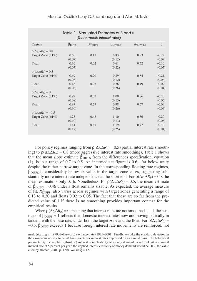
For policy regimes ranging from ρ(∆z,∆Rb) = 0.5 (partial interest rate smooth-ing) to ρ(∆z,∆Rb) = 0.8 (more aggressive interest rate smoothing), Table 1 showsthat the mean slope estimate βDIFFS from the differences specification, equation(1), is in a range of 0.7 to 0.5. An intermediate figure is 0.6—far below unitydespite the rather narrow target zone. In the corresponding floating-rate regimes,βDIFFS is considerably below its value in the target-zone cases, suggesting sub-stantially more interest rate independence at the short end. For ρ(∆z,∆Rb) = 0.8 themean estimate is only 0.16. Nonetheless, for ρ(∆z,∆Rb) = 0.5, the mean estimateof βDIFFS = 0.46 under a float remains sizable. As expected, the average measureof fit, R2
DIFFS, also varies across regimes with target zones generating a range of0.13 to 0.20 and floats 0.02 to 0.05. The fact that these are so far from the pre-dicted value of 1 if there is no smoothing provides important context for theempirical results.
When ρ(∆z,∆Rb) = 0, meaning that interest rates are not smoothed at all, the esti-mate of βDIFFS ≈ 1 reflects that domestic interest rates now are moving basically intandem with the base rate, under both the target zone and the float. For ρ(∆z,∆Rb) =−0.5, βDIFFS exceeds 1 because foreign interest rate movements are reinforced, not
Maurice Obstfeld, Jay C. Shambaugh, and Alan M. Taylor
84
mark (starting in 1999, dollar-euro) exchange rate (1975–2001). Finally, we take the standard deviation inthe exogenous noise v to be 20 basis points for interest rates expressed on an annual basis. The behavioralparameter η, the implicit (absolute) interest semielasticity of money demand, is set to 4. At a nominalinterest rate of 5 percent per year, the implied interest elasticity of money demand would be −0.2, the valuecited by Romer (2001, p. 470). We set ξ = 1.5.
Table 1. Simulated Estimates of β and θ(Three-month interest rates)
Regime βDIFFS R2DIFFS βLEVELS R2
LEVELS θ
ρ(∆z,∆Rb) = 0.8Target Zone (±1%) 0.50 0.13 0.83 0.83 −0.22
(0.07) (0.12) (0.07)Float 0.16 0.02 0.61 0.52 −0.10
(0.07) (0.22) (0.05)ρ(∆z,∆Rb) = 0.5Target Zone (±1%) 0.69 0.20 0.89 0.84 −0.21
(0.08) (0.12) (0.06)Float 0.46 0.05 0.76 0.49 −0.09
(0.08) (0.26) (0.04)ρ(∆z,∆Rb) = 0Target Zone (±1%) 0.99 0.33 1.00 0.86 −0.20
(0.08) (0.13) (0.06)Float 0.97 0.27 0.98 0.67 −0.09
(0.10) (0.26) (0.04)ρ(∆z,∆Rb) = −0.5Target Zone (±1%) 1.28 0.43 1.10 0.86 −0.20
(0.10) (0.13) (0.06)Float 1.44 0.47 1.19 0.77 −0.10
(0.17) (0.25) (0.04)
offset, by domestic policy. The effect is stronger under a float than under a targetzone. Under a float, the effects of fundamentals on the exchange rate, and hence, theinterest rate responses, are not muted by expected intervention at the band edges.
The results of estimating the levels specification, equation (5), are reported inthe column of Table 1 labeled βLEVELS. These results are as expected when the baseinterest rate, Rbit, has a unit root. The levels estimates β LEVELS are much closer tounity than β DIFFS under all policy settings, and as a result, the estimated differ-ences between the target zone and the float are much less evident than in the lesscompressed differences estimates. We have experimented with simulated sampleperiods out to 100 years and find that while the differences estimates remain quitestable, the levels estimates (as one would expect) move markedly in the directionof unity as the sample period is lengthened. The levels estimates obscure the con-trasts between regimes in finite samples, and will hide them entirely as the time-series sample grows arbitrarily long. The values of R2
LEVELS are high due to thecommon trend in foreign and domestic interest rates.
In practice we estimate equation (1) on a panel of annual year-average inter-est rate changes, so as to minimize international asymmetries caused by differentshort-term dynamic adjustment patterns to foreign interest rate changes. We pur-sue an additional estimation strategy, however, that focuses directly on the dynam-ics of adjustment. If the interest rate data are indeed statistically nonstationary, anerror-correction specification can be used to analyze the dynamics of monthlydata. In practice one cannot be sure the data are I(1) rather than I(0). To maintainan agnostic view on stationarity, we employ a technique proposed by Pesaran,Shin, and Smith (2001), henceforth PSS, in which an error-correction form is esti-mated but different critical values are applied to the I(1) and I(0) cases.11 Onlywhen test statistics lie in an intermediate range must inference rely on an assump-tion about the order of integration.
The PSS technique relies on the specification
(7)
where lags of ∆Rit and ∆Rbit are included as necessary and γ is a cointegratingcoefficient. The significance and absolute magnitude of the coefficient θ, whichwe expect to be negative, if local interest rates adjust back toward the base rateafter a shock, reflect the strength of the adjustment forces. In the monthly data weuse, a coefficient of θ = −0.5 would imply a half-life of one month. Other thingsbeing equal, faster adjustment is an indicator of a less autonomous monetary pol-icy. For nonstationary data we would expect γ = 1, in which case one could imposethat equality on the equation before estimating θ.
The final column of Table 1 reports mean simulated values of the estimate θfrom equation (7). The estimates average to around −0.2 under a target zone andabout −0.1 under a float, with the result fairly insensitive to the extent of short-runinterest rate smoothing. The implied half-lives of shocks are under three monthsfor a target zone but roughly seven months for floats.
∆ ∆R R c R R uit bit it bi t it= + + + −( ) +− −α β θ γ1 1, ,
MONETARY SOVEREIGNTY, EXCHANGE RATES, AND CAPITAL CONTROLS
85
11This technique is also used by Frankel, Schmukler, and Servén (2002).
III. Data
Interest Rate Data
To test the trilemma’s predictions, we must describe the different policy optionscountries are pursuing. As noted above, we view the short-term nominal interestrate as the instrument of a country’s monetary policy and the extent of comovementof the local nominal interest rate with a nominal base-country interest rate as an(inverse) expression of monetary policy autonomy.
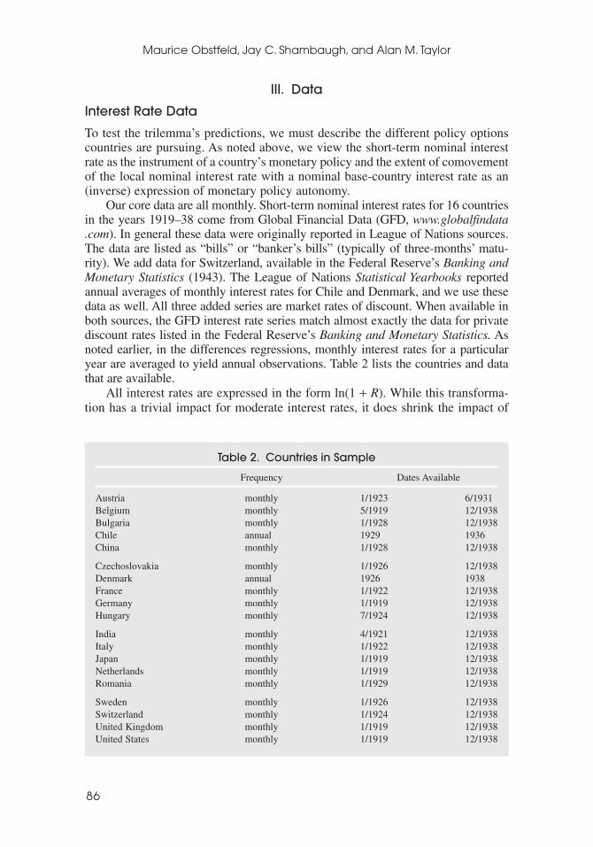
Our core data are all monthly. Short-term nominal interest rates for 16 countriesin the years 1919–38 come from Global Financial Data (GFD, www.globalfindata.com). In general these data were originally reported in League of Nations sources.The data are listed as “bills” or “banker’s bills” (typically of three-months’ matu-rity). We add data for Switzerland, available in the Federal Reserve’s Banking andMonetary Statistics (1943). The League of Nations Statistical Yearbooks reportedannual averages of monthly interest rates for Chile and Denmark, and we use thesedata as well. All three added series are market rates of discount. When available inboth sources, the GFD interest rate series match almost exactly the data for privatediscount rates listed in the Federal Reserve’s Banking and Monetary Statistics. Asnoted earlier, in the differences regressions, monthly interest rates for a particularyear are averaged to yield annual observations. Table 2 lists the countries and datathat are available.
All interest rates are expressed in the form ln(1 + R). While this transforma-tion has a trivial impact for moderate interest rates, it does shrink the impact of
Maurice Obstfeld, Jay C. Shambaugh, and Alan M. Taylor
86
Table 2. Countries in Sample
Frequency Dates Available
Austria monthly 1/1923 6/1931Belgium monthly 5/1919 12/1938Bulgaria monthly 1/1928 12/1938Chile annual 1929 1936China monthly 1/1928 12/1938
Czechoslovakia monthly 1/1926 12/1938Denmark annual 1926 1938France monthly 1/1922 12/1938Germany monthly 1/1919 12/1938Hungary monthly 7/1924 12/1938
India monthly 4/1921 12/1938Italy monthly 1/1922 12/1938Japan monthly 1/1919 12/1938Netherlands monthly 1/1919 12/1938Romania monthly 1/1929 12/1938
Sweden monthly 1/1926 12/1938Switzerland monthly 1/1924 12/1938United Kingdom monthly 1/1919 12/1938United States monthly 1/1919 12/1938
outliers. In addition, the German hyperinflation is removed to prevent the massiveinterest rate swings during that relatively short episode from overwhelming therest of the data. Thus, observations for Germany from 1923–25 are eliminated.
Because we are interested in comovements with the base interest rate, animportant choice is that of the center-country or base nominal interest rate. Undertypical post–World War II fixed exchange rate regimes, countries have pegged toother countries, thereby revealing their particular bases. In theory, however, amultilateral gold standard regime differs, in that monetary changes in any countryaffect the system as a whole, and there is symmetric adjustment. More practically,however, one thinks of a de facto center country, namely, Great Britain, at leastunder the pre-1914 gold standard. In contrast to the classical gold standard, though,there is no clear base country for the system as a whole during the interwar years.While the United States returned fully to the gold standard immediately after WorldWar I, it is not clear that the United States was the sole base for the system. Indeed,the U.S. dollar itself did not remain fixed against gold throughout the entire era(Franklin Roosevelt devalued the dollar-gold exchange rate in 1933). Sterling wasnot convertible into gold for much of the period; Britain remained on gold only forabout 77 months, so Britain is not an ideal base country either. France played amajor role in the setting of policies because of its successful attempt to amass largequantities of gold reserves, but it did not repeg to gold on a de jure basis until 1928,two years after the Poincaré macroeconomic stabilization, making it an inappropri-ate choice as a base country early on in the time period that we study. Because theUnited States and France held the majority of gold reserves, our default procedureis to use the U.S. interest rate for the early and late periods, and a combination ofU.S. and French rates for the years France is on a de jure gold standard.12 This baseinterest rate will be referred to below as the gold interest rate.13
Due to the lack of a clear center country, we consider a variety of base coun-try interest rates as robustness checks. We checked all cases using the U.S. inter-est rate alone, as well as considering the British interest rate as the base rate, as away of checking the assumption that Britain had ceased to be the center coun-try. We also tried varying the base by local country to allow for the fact that,especially after 1931, the system broke down into smaller spheres of influence.We followed the coding that Eichengreen and Irwin (1995) use to describe currencyblocs, dividing countries into Sterling countries (Denmark, India, Japan, and Sweden,using Britain as the base), Gold Bloc countries (Belgium, Italy, Netherlands, andSwitzerland, using France as the base), Reichsmark countries (Austria, Bulgaria,Czechoslovakia, Hungary, and Romania, using Germany as the base), and othercountries (China and Chile, using the United States as base).14 While the cross-base
MONETARY SOVEREIGNTY, EXCHANGE RATES, AND CAPITAL CONTROLS
87
12Mouré (2002) discusses how many view France’s gold policies as having had a strong impact on thesystem as a whole. This source also reports that France and the United States had the two largest nationalgold reserves and that, combined, they held 50 to 60 percent of the world’s total stock of gold reserves.
13For annual differences regressions, this is simply the average of the change in the U.S. and Frenchrates. For the levels analysis on monthly data, the U.S. rate is used up to 1928, and then that rate is adjustedgoing forward by the average change in the U.S. and French rates until 1936, after which it is adjusted bychanges in the U.S. rate alone.
14In addition, we tried both simply eliminating the base countries or including them using the UnitedStates as the base rate for France, Germany, and Britain.
comparisons are discussed below, we feel in general that the gold interest rate isthe most appropriate choice for the base rate.
Exchange Rate Regime Coding
The exchange rate regimes are classified based on both the legal commitment ofcountries to gold (the de jure status) as well as the de facto behavior of the exchangerate. De jure coding is based on the dates given by Obstfeld and Taylor (2003).The de jure status is in some sense a combination of the exchange rate regime andcapital control regime sides of the trilemma as countries are considered to be offgold if they restricted convertibility in any way. The de facto standard follows thecoding for the post–Bretton Woods era developed in Shambaugh (2004). We askwhether the monthly exchange rate stayed within ±2 percent bands over the courseof a year. In addition, single realignments are not considered breaks in the regimeas long as the transition is immediate from one peg to another. Finally, single-year pegs are dropped as they are quite likely a simple lack of volatility and it isunlikely that there exists either commitment on the government’s part or confi-dence in the market that the rate will not change.15 We use the categories “peg”and “nonpeg” to classify currency regimes so as to emphasize that countries with-out pegged rates may not be “pure” floats in which exchange rate management iseschewed. Countries with nonpegs simply do not peg completely (according toour metric).
Because there is no single base country to which countries peg, exchange ratesare tested for stability against gold by examining the exchange rate against the dol-lar during the dollar’s peg to gold, and against the French franc in the two-yearperiod (1933–34) of dollar instability against gold. This provides a full series ofcodes for the countries that stayed pegged to gold on a de facto basis.16 Exchangerate data come from GFD.
Capital Control Status
To conduct our empirical analysis of the trilemma, we also need to code countriesas to their use of capital controls. As mentioned, the de jure exchange rate regimesautomatically incorporate this criterion. De facto capital control classificationshave been created for more recent eras, but most are available only for a limitednumber of countries and a limited amount of time. Furthermore, some measuresrely on interest differentials (the variable upon which we focus) and thus are notappropriate for the present study. No other clear source has been used to describe
Maurice Obstfeld, Jay C. Shambaugh, and Alan M. Taylor
88
15When pursuing differences regressions, we also drop the first year of a peg to avoid differencinginterest rates across nonpegged and pegged observations. Shambaugh (2004) provides an extensive dis-cussion of different de facto classifications. Recent work by Reinhart and Rogoff (2004), which uses dataon parallel exchange rates, is not directly relevant to the present paper. Countries with parallel exchangemarkets employ capital controls to separate commercial from financial transactions, and for that reasonalone are likely to enjoy some degree of monetary independence.
16As an alternative, we also looked at the years the League of Nations listed a country as pegging to gold.The results are consistent with those reported below.
capital controls in this era before. We turn to two sources to generate our own cod-ing of capital controls. The League of Nations publication Legislation on Gold(1930) gives a history of when countries returned to gold convertibility, so we areable to code at what point after World War I countries opened their capital mar-kets to gold flows. In addition, the League of Nations’ Monetary Review (1938)provides a table that describes when countries put in place exchange controls inthe 1930s (Appendix Table 1, p. 107). Combining these sources gives us our mea-sure of capital controls. Clearly, this binary measure is imperfect in capturing therange of effectiveness that various controls may have had, but we feel that it pro-vides a useful indication of the countries trying to create breathing room by limit-ing cross-border financial flows.
Individual Country Episodes
For the dynamic time-series analysis based on specification (7), we study monthlydata on individual country/regime episodes. Two types of episodes are examined.First we look at the de jure coding, which gives us 13 pegged episodes and 21 nonpegged episodes (half of them occurring prior to the reconstituted gold stan-dard, and half after). We also use our exchange rate regime coding methodology togenerate a monthly classification of the currency regime in effect. We follow muchthe same method as for annual data, checking that the exchange rate has stayed within±2 percent bands over the preceding 12 months. We then combine this informationwith our dates for capital controls to generate four types of episode: open pegs, closedpegs, open nonpegs, and closed nonpegs. Brief episodes of less than three years areexcluded as too short to allow informative time-series inference. There are 11 openpegs, 3 closed pegs, 4 open nonpegs, and 3 closed nonpegs.
Unit Roots in Interest Rates
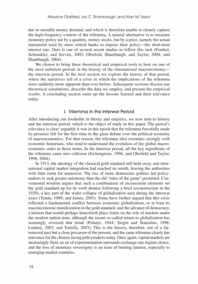
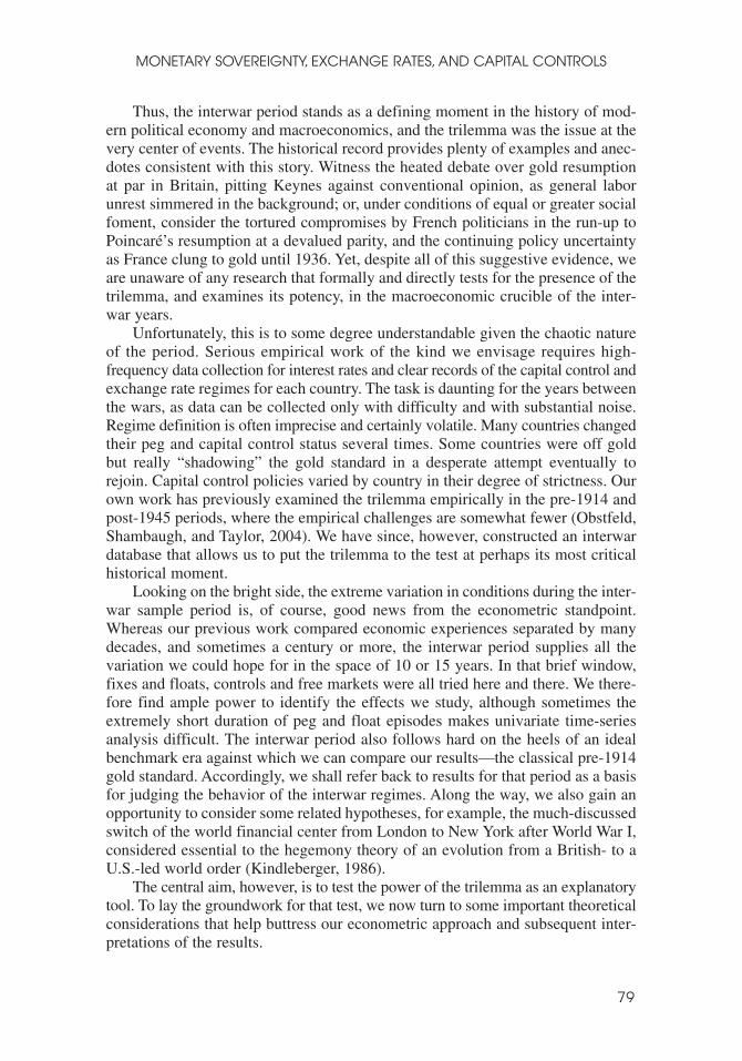
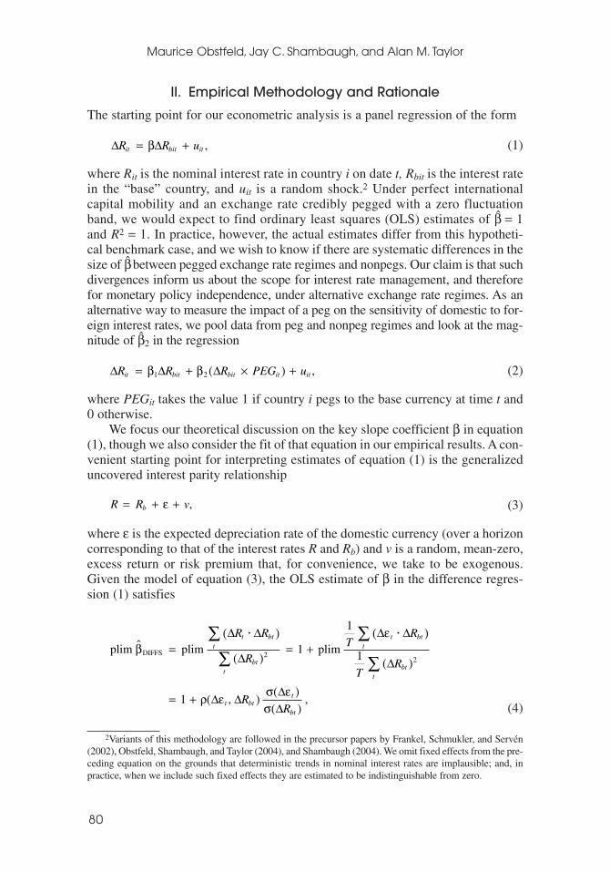
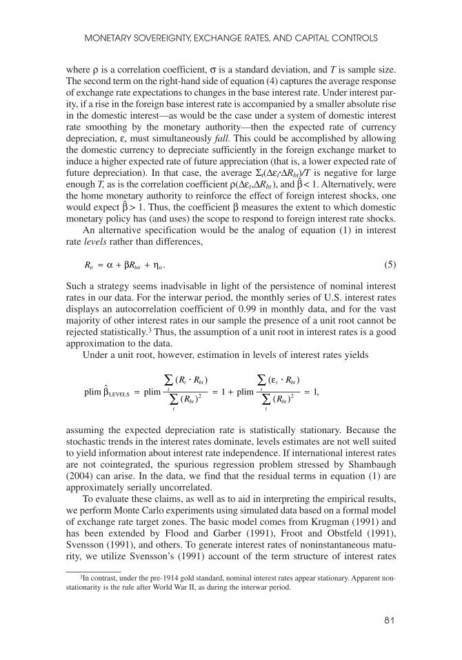
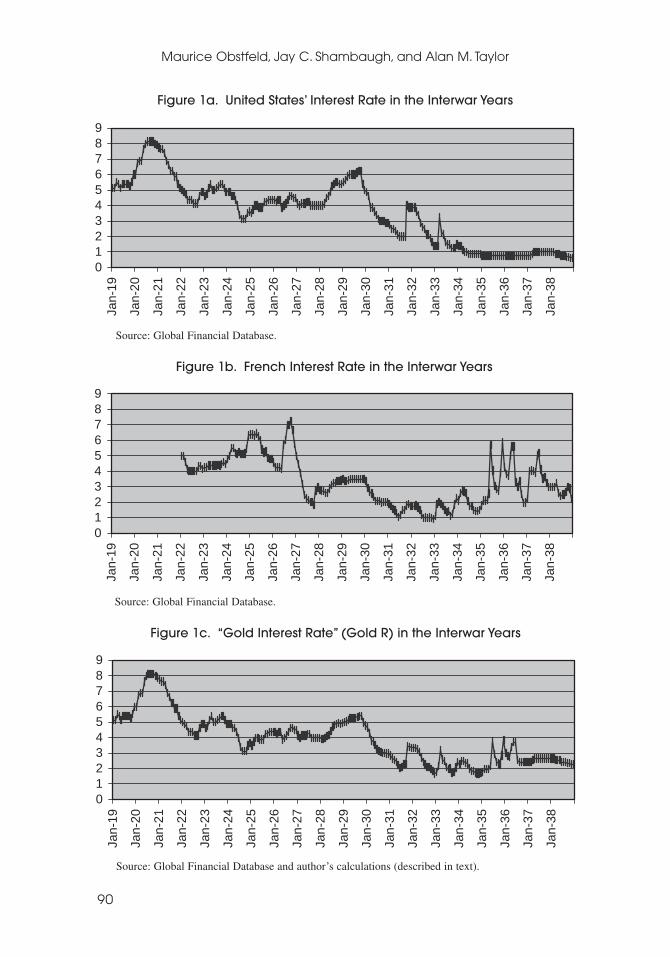
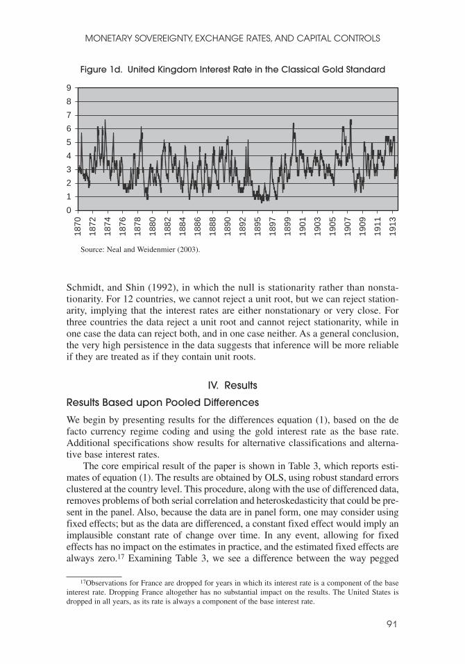
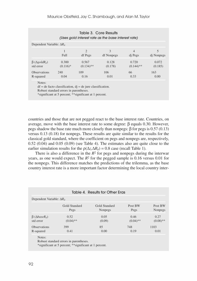
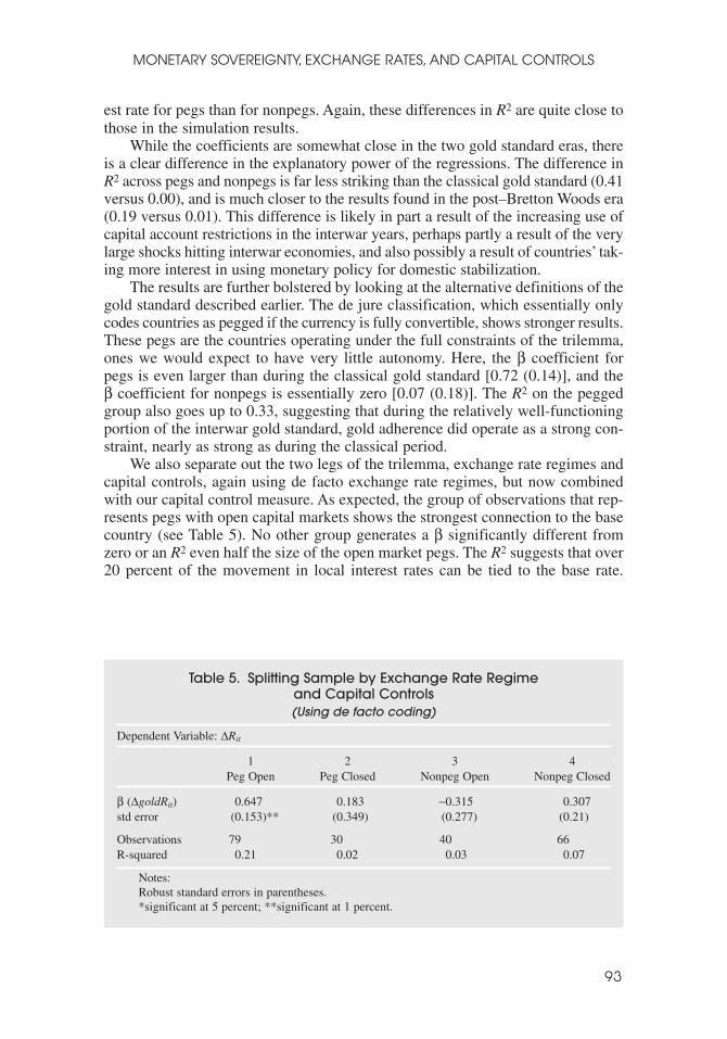
While the methodology section considers the fact that many time series of nominalinterest rate data are difficult to distinguish from unit roots, this is not necessarilytrue for the classical gold standard era. While showing persistence, the British inter-est rate, the clear base rate under the classical gold standard, is relatively stable asare the interest rates of most other gold standard countries. On the other hand, theinterwar years appear to resemble the Bretton Woods or post–Bretton Woods eras,in that the interest rates of most countries show very strong serial correlation.Figures 1a, 1b, and 1c show the interest rates for the United States, France, and thecombined gold interest rate. For comparison, Figure 1d shows Britain’s interest rateduring the classical gold standard.
Simple tests on monthly base and local interest rates back up this ocular evi-dence that interwar interest rates are highly persistent. The autocorrelation coeffi-cient for the U.S. rate is 0.99. The average autocorrelation coefficient for the othercountries is 0.96. More formally, we apply the unit root test suggested by Elliott,Rothenberg, and Stock (1996), using the modified Akaike Information Criterionof Ng and Perron (2001) to determine the appropriate number of lags to include.In addition, we test for stationarity using the KPSS test of Kwiatkowski, Phillips,
MONETARY SOVEREIGNTY, EXCHANGE RATES, AND CAPITAL CONTROLS
89
90
Maurice Obstfeld, Jay C. Shambaugh, and Alan M. Taylor
Figure 1a. United States’ Interest Rate in the Interwar Years
0123456789
Jan-
19
Jan-
20
Jan-
21
Jan-
22
Jan-
23
Jan-
24
Jan-
25
Jan-
26
Jan-
27
Jan-
28
Jan-
29
Jan-
30
Jan-
31
Jan-
32
Jan-
33
Jan-
34
Jan-
35
Jan-
36
Jan-
37
Jan-
38
Source: Global Financial Database.
Figure 1b. French Interest Rate in the Interwar Years
Source: Global Financial Database.
0123456789
Jan-
19
Jan-
20
Jan-
21
Jan-
22
Jan-
23
Jan-
24
Jan-
25
Jan-
26
Jan-
27
Jan-
28
Jan-
29
Jan-
30
Jan-
31
Jan-
32
Jan-
33
Jan-
34
Jan-
35
Jan-
36
Jan-
37
Jan-
38
Figure 1c. “Gold Interest Rate” (Gold R) in the Interwar Years
Source: Global Financial Database and author’s calculations (described in text).
0123456789
Jan-
19
Jan-
20
Jan-
21
Jan-
22
Jan-
23
Jan-
24
Jan-
25
Jan-
26
Jan-
27
Jan-
28
Jan-
29
Jan-
30
Jan-
31
Jan-
32
Jan-
33
Jan-
34
Jan-
35
Jan-
36
Jan-
37
Jan-
38
MONETARY SOVEREIGNTY, EXCHANGE RATES, AND CAPITAL CONTROLS
91
Schmidt, and Shin (1992), in which the null is stationarity rather than nonsta-tionarity. For 12 countries, we cannot reject a unit root, but we can reject station-arity, implying that the interest rates are either nonstationary or very close. Forthree countries the data reject a unit root and cannot reject stationarity, while inone case the data can reject both, and in one case neither. As a general conclusion,the very high persistence in the data suggests that inference will be more reliableif they are treated as if they contain unit roots.
IV. Results
Results Based upon Pooled Differences
We begin by presenting results for the differences equation (1), based on the defacto currency regime coding and using the gold interest rate as the base rate.Additional specifications show results for alternative classifications and alterna-tive base interest rates.
The core empirical result of the paper is shown in Table 3, which reports esti-mates of equation (1). The results are obtained by OLS, using robust standard errorsclustered at the country level. This procedure, along with the use of differenced data,removes problems of both serial correlation and heteroskedasticity that could be pre-sent in the panel. Also, because the data are in panel form, one may consider usingfixed effects; but as the data are differenced, a constant fixed effect would imply animplausible constant rate of change over time. In any event, allowing for fixedeffects has no impact on the estimates in practice, and the estimated fixed effects arealways zero.17 Examining Table 3, we see a difference between the way pegged
Figure 1d. United Kingdom Interest Rate in the Classical Gold Standard
0
1
2
3
4
5
6
7
8
918
70
1872
1874
1876
1878
1880
1882
1884
1886
1888
1890
1892
1895
1897
1899
1901
1903
1905
1907
1909
1911
1913
Source: Neal and Weidenmier (2003).
17Observations for France are dropped for years in which its interest rate is a component of the baseinterest rate. Dropping France altogether has no substantial impact on the results. The United States isdropped in all years, as its rate is always a component of the base interest rate.
countries and those that are not pegged react to the base interest rate. Countries, onaverage, move with the base interest rate to some degree: β equals 0.30. However,pegs shadow the base rate much more closely than nonpegs: β for pegs is 0.57 (0.13)versus 0.13 (0.18) for nonpegs. These results are quite similar to the results for theclassical gold standard, where the coefficient on pegs and nonpegs are, respectively,0.52 (0.04) and 0.05 (0.09) (see Table 4). The estimates also are quite close to theearlier simulation results for the ρ(∆z,∆Rb) = 0.8 case (recall Table 1).
There is also a difference in the R2 for pegs and nonpegs during the interwaryears, as one would expect. The R2 for the pegged sample is 0.16 versus 0.01 forthe nonpegs. This difference matches the predictions of the trilemma, as the basecountry interest rate is a more important factor determining the local country inter-
Maurice Obstfeld, Jay C. Shambaugh, and Alan M. Taylor
92
Table 3. Core Results(Uses gold interest rate as the base interest rate)
Dependent Variable: ∆Rit
1 2 3 4 5Full df Pegs df Nonpegs dj Pegs dj Nonpegs
β (∆goldRit) 0.300 0.567 0.128 0.720 0.072std error (0.116)* (0.134)** (0.178) (0.144)** (0.185)
Observations 240 109 106 66 163R-squared 0.04 0.16 0.01 0.33 0.00
Notes:df = de facto classification, dj = de jure classification.Robust standard errors in parentheses.*significant at 5 percent; **significant at 1 percent.
Table 4. Results for Other Eras
Dependent Variable: ∆Rit
Gold Standard Gold Standard Post BW Post BWPegs Nonpegs Pegs Nonpegs
β (∆baseRit) 0.52 0.05 0.46 0.27std error (0.04)** (0.09) (0.04)** (0.08)**
Observations 399 85 748 1103R-squared 0.41 0.00 0.19 0.01
Notes:Robust standard errors in parentheses.*significant at 5 percent; **significant at 1 percent.
MONETARY SOVEREIGNTY, EXCHANGE RATES, AND CAPITAL CONTROLS
93
Table 5. Splitting Sample by Exchange Rate Regime and Capital Controls(Using de facto coding)
Dependent Variable: ∆Rit
1 2 3 4Peg Open Peg Closed Nonpeg Open Nonpeg Closed
β (∆goldRit) 0.647 0.183 −0.315 0.307std error (0.153)** (0.349) (0.277) (0.21)
Observations 79 30 40 66R-squared 0.21 0.02 0.03 0.07
Notes:Robust standard errors in parentheses.*significant at 5 percent; **significant at 1 percent.
est rate for pegs than for nonpegs. Again, these differences in R2 are quite close tothose in the simulation results.
While the coefficients are somewhat close in the two gold standard eras, thereis a clear difference in the explanatory power of the regressions. The difference inR2 across pegs and nonpegs is far less striking than the classical gold standard (0.41versus 0.00), and is much closer to the results found in the post–Bretton Woods era(0.19 versus 0.01). This difference is likely in part a result of the increasing use ofcapital account restrictions in the interwar years, perhaps partly a result of the verylarge shocks hitting interwar economies, and also possibly a result of countries’ tak-ing more interest in using monetary policy for domestic stabilization.
The results are further bolstered by looking at the alternative definitions of thegold standard described earlier. The de jure classification, which essentially onlycodes countries as pegged if the currency is fully convertible, shows stronger results.These pegs are the countries operating under the full constraints of the trilemma,ones we would expect to have very little autonomy. Here, the β coefficient forpegs is even larger than during the classical gold standard [0.72 (0.14)], and the β coefficient for nonpegs is essentially zero [0.07 (0.18)]. The R2 on the peggedgroup also goes up to 0.33, suggesting that during the relatively well-functioningportion of the interwar gold standard, gold adherence did operate as a strong con-straint, nearly as strong as during the classical period.
We also separate out the two legs of the trilemma, exchange rate regimes andcapital controls, again using de facto exchange rate regimes, but now combinedwith our capital control measure. As expected, the group of observations that rep-resents pegs with open capital markets shows the strongest connection to the basecountry (see Table 5). No other group generates a β significantly different fromzero or an R2 even half the size of the open market pegs. The R2 suggests that over20 percent of the movement in local interest rates can be tied to the base rate.
Thus, we see it is the combination of a fixed exchange rate and open capital mar-kets that seems to generate the loss of autonomy. When countries either float orclose their capital markets, they cease to follow the base as closely.18
Our interpretation is not without caveats, however. We cannot state clearlythat the trilemma is forcing countries to follow the base because these resultscould be the consequence of pegged countries simply choosing to follow the baseor experiencing shocks highly correlated with those hitting the base country.Previous work on the post–Bretton Woods era assumes a variety of base interestrates in a given time period, and thus allows the inclusion of time controls; dis-tance and trade-share controls have been included as well. The currency regimeand capital control regime variables still show strong impacts on the degree towhich a country follows the base (Shambaugh, 2004).
Table 5 contains an apparent anomaly, though. The closed capital market non-pegs should be the group with the greatest monetary freedom. While all groupsexcept open pegs should be able to pursue autonomous monetary policy to somedegree, both conventional wisdom and results from other eras (see Obstfeld,Shambaugh, and Taylor, 2004) would suggest that the closed market nonpegs shouldbe the least linked to the base. There should be very little pressure on them torespond to the base interest rate, as they should have achieved substantial auton-omy both through shutting capital markets and by not pegging. We find, though,that this group has a larger (though still statistically insignificant) estimated βcoefficient than do open nonpegs or closed pegs, and an R2 of 0.07. This patternindicates a stronger connection for this group than for the closed pegs or the opencapital market nonpegs, and it is robust across a wide variety of base interest ratedefinitions and regime classifications. We return to this curious finding when weexamine different time periods within the interwar sample.
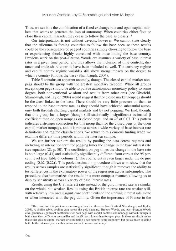
We can further explore the results by pooling the data across regimes andincluding an interaction term for pegging times the change in the base interest rate(see equation (2), p. 80). The coefficient on peg times the change in the base rateis both large (0.43) and statistically significantly different from zero at the 95 per-cent level (see Table 6, column 1). The coefficient is even larger under the de jurecoding (0.62 (0.22)). This pooled estimation procedure allows us to show that theresults across samples are statistically significant, though it removes the ability totest differences in the explanatory power of the regression across subsamples. Theprocedure also summarizes the results in a more compact manner, allowing us todisplay sensitivity across a variety of base interest rates.
Results using the U.S. interest rate instead of the gold interest rate are similaron the whole, but weaker. Results using the British interest rate are weaker still,with relatively low and insignificant coefficients on the sterling interest rate aloneor when interacted with the peg dummy. Given the importance of France in the
Maurice Obstfeld, Jay C. Shambaugh, and Alan M. Taylor
94
18The results on this point are even stronger than for other eras (see Obstfeld, Shambaugh, and Taylor,2004). A similar table, pooling data across the gold standard, Bretton Woods, and post–Bretton Woodseras, generates significant coefficients for both pegs with capital controls and nonpegs without, though inboth cases the coefficients are smaller and the R2 much lower than for open pegs. In those results, it seemsthat either closing capital markets or eliminating a peg restores some autonomy, but not as much as doingboth. In the interwar years, either action seems to restore autonomy.
system and the fact that the United States broke from gold at one point, it is notsurprising that the gold interest rate shows a stronger sway over pegged countries’interest rates than does the dollar rate alone. Likewise, given Britain’s relativelybrief tenure in the interwar gold standard, it is not surprising that the country doesnot appear to have provided a base interest rate for the system. The weak inter-national connections to Britain’s interest rate do, however, support the view thatafter World War I, London was no longer the unrivaled center of global financialpower. This finding is therefore consistent with Kindleberger’s (1986) argumentthat a shift in hegemonic financial power was in progress during the interwaryears. The regressions breaking the base interest rate into different rates for dif-ferent countries are reported in column 5 of Table 6. It seems that either the U.S.rate alone or the U.S.-French rate in combination holds a much stronger sway overcountries than the various bases that may have been regional or historical leaders.19
With each interest rate base, the divided sample results (analogous to those inTable 3) yield a significant coefficient on the peg sample and an insignificant oneon the nonpeg sample. The coefficients on nonpegs are sometimes estimated soimprecisely, however, that the differences across groups are not statistically sig-nificant for every different base interest rate when the data are pooled.
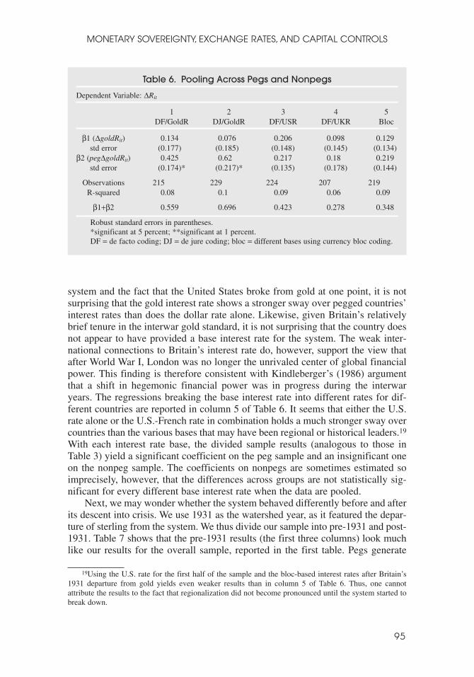
Next, we may wonder whether the system behaved differently before and afterits descent into crisis. We use 1931 as the watershed year, as it featured the depar-ture of sterling from the system. We thus divide our sample into pre-1931 and post-1931. Table 7 shows that the pre-1931 results (the first three columns) look muchlike our results for the overall sample, reported in the first table. Pegs generate
MONETARY SOVEREIGNTY, EXCHANGE RATES, AND CAPITAL CONTROLS
95
19Using the U.S. rate for the first half of the sample and the bloc-based interest rates after Britain’s1931 departure from gold yields even weaker results than in column 5 of Table 6. Thus, one cannotattribute the results to the fact that regionalization did not become pronounced until the system started tobreak down.
Table 6. Pooling Across Pegs and Nonpegs
Dependent Variable: ∆Rit
1 2 3 4 5DF/GoldR DJ/GoldR DF/USR DF/UKR Bloc
β1 (∆goldRit) 0.134 0.076 0.206 0.098 0.129std error (0.177) (0.185) (0.148) (0.145) (0.134)
β2 (peg∆goldRit) 0.425 0.62 0.217 0.18 0.219std error (0.174)* (0.217)* (0.135) (0.178) (0.144)
Observations 215 229 224 207 219R-squared 0.08 0.1 0.09 0.06 0.09
β1+β2 0.559 0.696 0.423 0.278 0.348
Robust standard errors in parentheses.*significant at 5 percent; **significant at 1 percent.DF = de facto coding; DJ = de jure coding; bloc = different bases using currency bloc coding.
higher coefficients and higher R2 than nonpegs and the predicted target-zonecoefficients in the neighborhood of 0.6 still arise. On the other hand, the post-1931results are radically different. Both pegs and nonpegs show coefficients signifi-cantly different from zero and in fact greater than 1, although we cannot reject thatthey are different from the frequently seen baseline estimate of 0.6. In addition, thesource of the anomaly in Table 5, which we discussed earlier, comes to light. Theclosed capital market nonpegs show a coefficient significantly different from zero,indeed well above 1, and an R2 exceeding 0.2. When splitting the data into suchnarrow groups, we arrive at a small number of observations (35 in the case of theclosed nonpegs after 1931). Still, despite the small number of observations, thisresult is statistically significant at the 99 percent level.
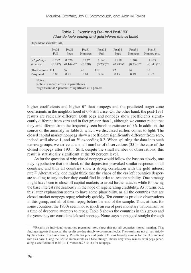
As for the question of why closed nonpegs would follow the base so closely, onemay hypothesize that the shock of the depression provoked similar responses in allcountries, and thus all countries show a strong correlation with the gold interestrate.20 Alternatively, one might think that the chaos of the era left countries desper-ate to cling to any anchor they could find in order to restore stability. One strategymight have been to close off capital markets to avoid further attacks while followingthe base interest rate zealously in the hope of regenerating credibility. As it turns out,this latter explanation seems to have some plausibility, as all the countries that areclosed market nonpegs repeg relatively quickly. Ten countries produce observationsin this group, and all of them repeg before the end of the sample. Thus, at least forsome countries, the 1930s seem not so much an era of pure monetary nationalism, asa time of desperate attempts to repeg. Table 8 shows the countries in this group andthe years they are considered closed nonpegs. None stays nonpegged straight through
Maurice Obstfeld, Jay C. Shambaugh, and Alan M. Taylor
96
20Results on individual countries, presented next, show that not all countries moved together. Thatfinding suggests that not all the results are due simply to common shocks. The results are not driven strictlyby the choice of a base country. Results for pre- and post-1931 look broadly similar for the U.S. interestrate as a base. Using the British interest rate as a base, though, shows very weak results, with pegs gener-ating a coefficient of 0.25 (0.11) versus 0.27 (0.16) for nonpegs.
Table 7. Examining Pre- and Post-1931(Uses de facto coding and gold interest rate as base)
Dependent Variable: ∆Rit
Pre31 Pre31 Pre31 Post31 Post31 Post31 Post31Full Pegs Nonpegs Full Pegs Nonpegs Nonpeg clsd
β(∆goldRit) 0.292 0.576 0.122 1.146 1.218 1.304 1.353std error (0.147) (0.144)** (0.220) (0.206)** (0.483)* (0.359)** (0.341)**
Observations 111 56 46 112 42 54 35R-squared 0.05 0.21 0.01 0.14 0.15 0.19 0.23
Notes:Robust standard errors in parentheses.*significant at 5 percent; **significant at 1 percent.
MONETARY SOVEREIGNTY, EXCHANGE RATES, AND CAPITAL CONTROLS
97
Table 8. Observations That Are Closed Nonpegs Post-1931
Country Years
Bulgaria 1933–36China 1934–35, 1938Czechoslovakia 1933–36Germany 1933Hungary 1933, 1936
Italy 1934–36Japan 1932–35, 1938Romania 1933–36Chile 1932–36Denmark 1932–34, 1938
(text continues on page 104)
to 1938; all restore a peg at some point. Many—for example, Czechoslovakia—appear to be freer than they were in reality, as they peg briefly during some of theyears they are listed as nonpegs, but not consistently enough to be considered a pegin those years. We return to these questions in the levels analysis.
Time-Series Levels Analysis
We can explore these issues further by examining individual country relationshipswith the base interest rate. To do so we use the PSS methodology to test for theexistence of levels relationships between interest rates, simultaneously examiningthe dynamics of adjustment.
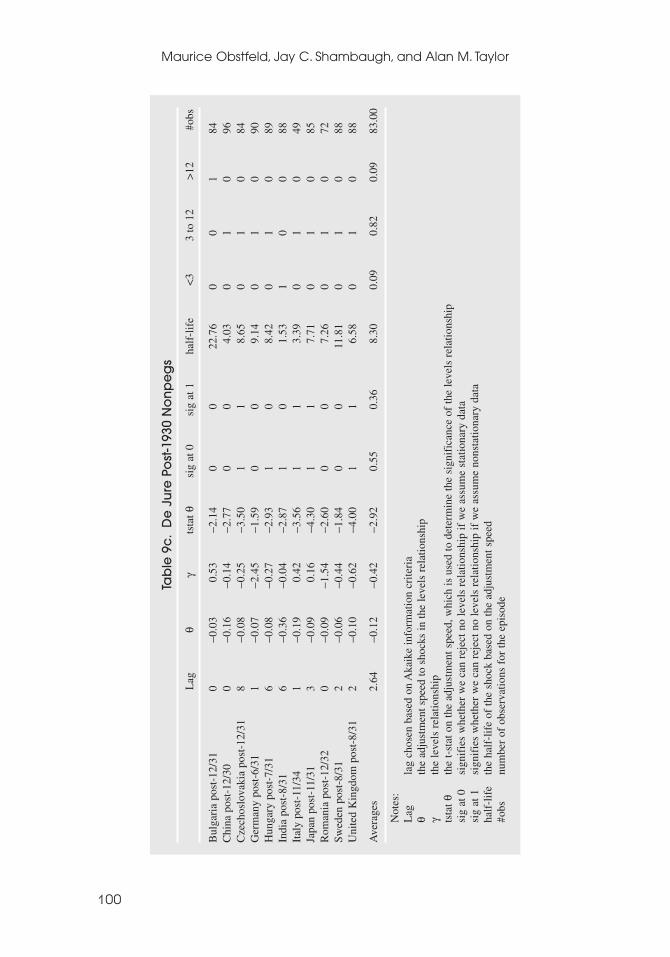
Table 9 shows the individual results grouped by type of episode. The de jureresults have the advantage of only having to group countries by one measure.We examine 3 groups, pegs, nonpegs before 1931, and nonpegs starting in 1931.It appears that the relationship seen at the pooled panel level still holds at theindividual level. By and large, the pegs seem to follow the base rate (Table 9ashows the gold interest rate results). Six out of the 13 episodes are significant atboth the I(1) and I(0) critical values, the average cointegrating coefficient is0.53 and the average half-life of adjustment is 5 months. In addition, only 1 episode(Germany) has a backwards level relationship (that is, γ < 0) and only one other(Italy) has a half-life of over 12 months. Nine out of the 13 have a levels rela-tionship of the correct sign and half-lives below six months.
Nonpegs do not show such a close relationship. Of the pre-1931 nonpegs, only1 has a levels relationship that is both significant and in the correct direction. Theaverage coefficient is −0.01, and the average adjustment half-life is 29 months.Also, 2 of the 8 cases have backwards levels relationships, and 3 more, have adjust-ment half-lives in excess of 12 months. Only China and the United Kingdom showmuch of a connection to the base rate. Post-1930 nonpegs show almost no connec-tion at all with the gold interest rate. While 2 of the 11 have significant levels rela-

Maurice Obstfeld, Jay C. Shambaugh, and Alan M. Taylor
98
Tab
le 9
a.
De
Ju
re P
eg
s to
Go
ld In
tere
st R
ate
Lag
θγ
tsta
t θsi
g at
0si
g at
1ha
lf-l
ife
<3
3 to
12
>12
#obs
Aus
tria
3/2
5–9/
311
−0.1
00.
31−3
.47
11
6.31
01
076
Bel
gium
10/
26–2
/35
1−0
.23
0.61
−5.1
41
12.
711
00
101
Bul
gari
a 4/
28–1
2/31
0−0
.12
0.60
−1.6
40
05.
370
10
44C
zech
oslo
vaki
a 1/
29–1
2/31
5−0
.72
0.40
−2.8
10
00.
541
00
36G
erm
any
10/2
4–6/
313
−0.1
8−0
.75
−4.4
81
13.
510
10
81H
unga
ry 4
/25–
7/31
0−0
.12
0.43
−4.1
01
15.
470
10
76In
dia
3/27
–8/3
11
−0.3
00.
72−3
.76
11
1.97
10
054
Ital
y 2/
28–1
1/34
1−0
.05
1.18
−1.7
60
013
.24
00
183
Net
herl
ands
4/2
5–8/
362
−0.2
31.
03−3
.39
11
2.69
10
013
7R
oman
ia 1
/29–
12/3
20
−0.1
60.
98−2
.08
00
3.98
01
044
Swed
en 3
/24–
8/31
0−0
.26
0.53
−2.7
20
02.
321
00
67Sw
itzer
land
1/2
5–12
/36
1−0
.06
0.52
−2.3
10
011
.20
01
014
4U
nite
d K
ingd
om 4
/25–
8/31
0−0
.15
0.40
−1.8
10
04.
360
10
77
Ave
rage
s−0
.21
0.53
−3.0
30.
460.
464.
900.
380.
540.
0878
.46
Not
es:
Lag
lag
chos
en b
ased
on
Aka
ike
info
rmat
ion
crite
ria
θth
e ad
just
men
t spe
ed to
sho
cks
in th
e le
vels
rel
atio
nshi
pγ
the
leve
ls r
elat
ions
hip
tsta
t θth
e t-
stat
on
the
adju
stm
ent s
peed
, whi
ch is
use
d to
det
erm
ine
the
sign
ific
ance
of
the
leve
ls r
elat
ions
hip
sig
at 0
sign
ifie
s w
heth
er w
e ca
n re
ject
no
leve
ls r
elat
ions
hip
if w
e as
sum
e st
atio
nary
dat
asi
g at
1si
gnif
ies
whe
ther
we
can
reje
ct n
o le
vels
rel
atio
nshi
p if
we
assu
me
nons
tatio
nary
dat
aha
lf-l
ife
the
half
-lif
e of
the
shoc
k ba
sed
on th
e ad
just
men
t spe
ed#o
bsnu
mbe
r of
obs
erva
tions
for
the
epis
ode

MONETARY SOVEREIGNTY, EXCHANGE RATES, AND CAPITAL CONTROLS
99
Tab
le 9
b.
De
Ju
re P
re-1
931
No
np
eg
s
Lag
θγ
tsta
t θsi
g at
0si
g at
1ha
lf-l
ife
<3
3 to
12
>12
#obs
Bel
gium
pre
-10/
260
−0.0
20.
17−0
.68
00
29.7
90
01
88C
hina
pre
-193
10
−0.1
60.
79−1
.20
00
3.95
01
035
Indi
a up
to 2
/27
1−0
.24
−0.5
4−3
.86
11
2.49
10
069
Ital
y up
to 1
/28
1−0
.03
−1.7
8−1
.50
00
25.3
20
01
70Ja
pan
up to
12/
290
−0.0
10.
20−0
.28
00
138.
280
01
131
Net
herl
ands
up
to 3
/25
1−0
.41
0.13
−5.0
51
11.
321
00
73Sw
itzer
land
up
to 1
2/24
0−0
.03
0.29
−2.0
70
022
.01
00
171
Uni
ted
Kin
gdom
up
to 3
/25
0−0
.08
0.58
−1.3
30
08.
770
10
74
Ave
rage
s−0
.12
−0.0
2−2
.00
0.25
0.25
28.9
90.
250.
250.
5076
.38
Not
es:
Lag
lag
chos
en b
ased
on
Aka
ike
info
rmat
ion
crite
ria
θth
e ad
just
men
t spe
ed to
sho
cks
in th
e le
vels
rel
atio
nshi
pγ
the
leve
ls r
elat
ions
hip
tsta
t θth
e t-
stat
on
the
adju
stm
ent s
peed
, whi
ch is
use
d to
det
erm
ine
the
sign
ific
ance
of
the
leve
ls r
elat
ions
hip
sig
at 0
sign
ifie
s w
heth
er w
e ca
n re
ject
no
leve
ls r
elat
ions
hip
if w
e as
sum
e st
atio
nary
dat
asi
g at
1si
gnif
ies
whe
ther
we
can
reje
ct n
o le
vels
rel
atio
nshi
p if
we
assu
me
nons
tatio
nary
dat
aha
lf-l
ife
the
half
-lif
e of
the
shoc
k ba
sed
on th
e ad
just
men
t spe
ed#o
bsnu
mbe
r of
obs
erva
tions
for
the
epis
ode
Maurice Obstfeld, Jay C. Shambaugh, and Alan M. Taylor
100
Tab
le 9
c.
De
Ju
re P
ost
-193
0 N
on
pe
gs
Lag
θγ
tsta
t θsi
g at
0si
g at
1ha
lf-l
ife
<3
3 to
12
>12
#obs
Bul
gari
a po
st-1
2/31
0−0
.03
0.53
−2.1
40
022
.76
00
184
Chi
na p
ost-
12/3
00
−0.1
6−0
.14
−2.7
70
04.
030
10
96C
zech
oslo
vaki
a po
st-1
2/31
8−0
.08
−0.2
5−3
.50
11
8.65
01
084
Ger
man
y po
st-6
/31
1−0
.07
−2.4
5−1
.59
00
9.14
01
090
Hun
gary
pos
t-7/
316
−0.0
8−0
.27
−2.9
31
08.
420
10
89In
dia
post
-8/3
16
−0.3
6−0
.04
−2.8
71
01.
531
00
88It
aly
post
-11/
341
−0.1
90.
42−3
.56
11
3.39
01
049
Japa
n po
st-1
1/31
3−0
.09
0.16
−4.3
01
17.
710
10
85R
oman
ia p
ost-
12/3
20
−0.0
9−1
.54
−2.6
00
07.
260
10
72Sw
eden
pos
t-8/
312
−0.0
6−0
.44
−1.8
40
011
.81
01
088
Uni
ted
Kin
gdom
pos
t-8/
312
−0.1
0−0
.62
−4.0
01
16.
580
10
88
Ave
rage
s2.
64−0
.12
−0.4
2−2
.92
0.55
0.36
8.30
0.09
0.82
0.09
83.0
0
Not
es:
Lag
lag
chos
en b
ased
on
Aka
ike
info
rmat
ion
crite
ria
θth
e ad
just
men
t spe
ed to
sho
cks
in th
e le
vels
rel
atio
nshi
pγ
the
leve
ls r
elat
ions
hip
tsta
t θth
e t-
stat
on
the
adju
stm
ent s
peed
, whi
ch is
use
d to
det
erm
ine
the
sign
ific
ance
of
the
leve
ls r
elat
ions
hip
sig
at 0
sign
ifie
s w
heth
er w
e ca
n re
ject
no
leve
ls r
elat
ions
hip
if w
e as
sum
e st
atio
nary
dat
asi
g at
1si
gnif
ies
whe
ther
we
can
reje
ct n
o le
vels
rel
atio
nshi
p if
we
assu
me
nons
tatio
nary
dat
aha
lf-l
ife
the
half
-lif
e of
the
shoc
k ba
sed
on th
e ad
just
men
t spe
ed#o
bsnu
mbe
r of
obs
erva
tions
for
the
epis
ode

MONETARY SOVEREIGNTY, EXCHANGE RATES, AND CAPITAL CONTROLS
101
Tab
le 9
d.
De
Fa
cto
Op
en
Ca
pita
l Ma
rke
t Pe
gs
Lag
θγ
tsta
t θsi
g at
0si
g at
1ha
lf-l
ife
<3
3 to
12
>12
#obs
Aus
tria
1/2
4–9/
315
−0.0
31.
15−1
.36
00
20.0
40
01
90B
elgi
um 8
/27–
2/33
0−0
.12
0.57
−2.0
00
05.
330
10
67C
zech
2/2
7–9/
311
−0.1
40.
10−1
.46
00
4.70
01
056
Fran
ce 8
/28–
9/36
0−0
.06
0.47
−1.7
90
011
.40
01
098
Ger
man
y 11
/25–
6/31
0−0
.21
0.15
−3.8
91
12.
881
00
68H
unga
ry 1
1/26
–6/3
16
−0.3
80.
87−3
.45
11
1.45
10
056
Indi
a 12
/25–
8/31
2−0
.34
0.89
−4.5
11
11.
681
00
69It
aly
12/2
8–3/
341
−0.0
51.
50−1
.24
00
12.9
80
01
64N
ethe
rlan
ds 1
0/25
–9/3
62
−0.2
21.
00−3
.21
10
2.82
10
013
2Sw
eden
1/2
6–8/
310
−0.2
60.
53−2
.72
00
2.32
10
067
Switz
erla
nd 8
/25–
8/36
1−0
.05
0.44
−1.8
50
014
.09
00
113
4U
nite
d K
ingd
om 1
/26–
8/31
0−0
.12
0.16
−1.3
70
05.
520
10
68Sw
itzer
land
(or
ig)
8/25
–9/3
63
−0.0
60.
14−2
.25
00
10.6
50
10
134
Ave
rage
s1.
64−0
.17
0.67
−2.4
60.
360.
276.
710.
450.
270.
2779
.18
Not
es:
Lag
lag
chos
en b
ased
on
Aka
ike
info
rmat
ion
crite
ria
θth
e ad
just
men
t spe
ed to
sho
cks
in th
e le
vels
rel
atio
nshi
pγ
the
leve
ls r
elat
ions
hip
tsta
t θth
e t-
stat
on
the
adju
stm
ent s
peed
, whi
ch is
use
d to
det
erm
ine
the
sign
ific
ance
of
the
leve
ls r
elat
ions
hip
sig
at 0
sign
ifie
s w
heth
er w
e ca
n re
ject
no
leve
ls r
elat
ions
hip
if w
e as
sum
e st
atio
nary
dat
asi
g at
1si
gnif
ies
whe
ther
we
can
reje
ct n
o le
vels
rel
atio
nshi
p if
we
assu
me
nons
tatio
nary
dat
aha
lf-l
ife
the
half
-lif
e of
the
shoc
k ba
sed
on th
e ad
just
men
t spe
ed#o
bsnu
mbe
r of
obs
erva
tions
for
the
epis
ode
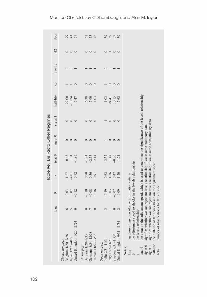
Maurice Obstfeld, Jay C. Shambaugh, and Alan M. Taylor
102
Tab
le 9
e.
De
Fa
cto
Oth
er
Reg
ime
s
Lag
θγ
tsta
t θsi
g at
0si
g at
1ha
lf-l
ife
<3
3 to
12
>12
#obs
Clo
sed
nonp
egs
Bel
gium
1/2
0–7/
266
0.03
−1.2
70.
430
0−2
7.00
10
079
Japa
n 12
/23–
4/27
50.
07−4
.01
1.01
00
−10.
241
00
41U
nite
d K
ingd
om 1
/20–
11/2
40
−0.1
20.
92−1
.86
00
5.47
01
059
Clo
sed
pegs
Bul
gari
a 1/
28–3
/33
0−0
.10
0.90
−1.8
40
06.
380
10
62G
erm
any
8/34
–12/
387
−0.0
80.
36−2
.33
00
7.90
01
053
Rom
ania
6/2
9–3/
330
−0.1
60.
91−2
.14
00
4.03
01
046
Ope
n no
npeg
sIn
dia
9/31
–11/
343
−0.4
90.
62−3
.57
11
1.03
10
039
Ital
y 1/
22–1
1/27
1−0
.03
−1.8
6−1
.47
00
24.4
10
01
69Sw
eden
9/3
1–11
/34
0−0
.07
0.47
−0.7
60
010
.15
01
039
Uni
ted
Kin
gdom
9/3
1–11
/34
2−0
.09
−1.2
0−1
.21
00
7.62
01
039
Not
es:
Lag
lag
chos
en b
ased
on
Aka
ike
info
rmat
ion
crite
ria
θth
e ad
just
men
t spe
ed to
sho
cks
in th
e le
vels
rel
atio
nshi
pγ
the
leve
ls r
elat
ions
hip
tsta
t θth
e t-
stat
on
the
adju
stm
ent s
peed
, whi
ch is
use
d to
det
erm
ine
the
sign
ific
ance
of
the
leve
ls r
elat
ions
hip
sig
at 0
sign
ifie
s w
heth
er w
e ca
n re
ject
no
leve
ls r
elat
ions
hip
if w
e as
sum
e st
atio
nary
dat
asi
g at
1si
gnif
ies
whe
ther
we
can
reje
ct n
o le
vels
rel
atio
nshi
p if
we
assu
me
nons
tatio
nary
dat
aha
lf-l
ife
the
half
-lif
e of
the
shoc
k ba
sed
on th
e ad
just
men
t spe
ed#o
bsnu
mbe
r of
obs
erva
tions
for
the
epis
ode
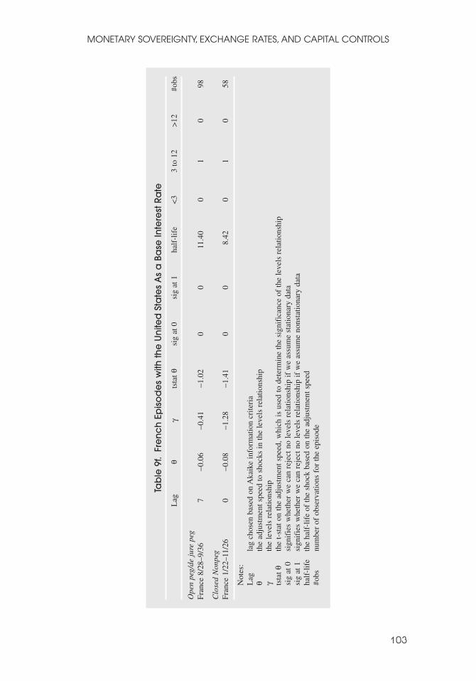
MONETARY SOVEREIGNTY, EXCHANGE RATES, AND CAPITAL CONTROLS
103
Tab
le 9
f.Fr
en
ch
Ep
iso
de
s w
ith th
e U
nite
d S
tate
s A
s a
Ba
se In
tere
st R
ate
Lag
θγ
tsta
t θsi
g at
0si
g at
1ha
lf-l
ife
<3
3 to
12
>12
#obs
Ope
n pe
g/de
jur
e pe
gFr
ance
8/2
8–9/
367
−0.0
6−0
.41
−1.0
20
011
.40
01
098
Clo
sed
Non
peg
Fran
ce 1
/22–
11/2
60
−0.0
8−1
.28
−1.4
10
08.
420
10
58
Not
es:
Lag
lag
chos
en b
ased
on
Aka
ike
info
rmat
ion
crite
ria
θth
e ad
just
men
t spe
ed to
sho
cks
in th
e le
vels
rel
atio
nshi
pγ
the
leve
ls r
elat
ions
hip
tsta
t θth
e t-
stat
on
the
adju
stm
ent s
peed
, whi
ch is
use
d to
det
erm
ine
the
sign
ific
ance
of
the
leve
ls r
elat
ions
hip
sig
at 0
sign
ifie
s w
heth
er w
e ca
n re
ject
no
leve
ls r
elat
ions
hip
if w
e as
sum
e st
atio
nary
dat
asi
g at
1si
gnif
ies
whe
ther
we
can
reje
ct n
o le
vels
rel
atio
nshi
p if
we
assu
me
nons
tatio
nary
dat
aha
lf-l
ife
the
half
-lif
e of
the
shoc
k ba
sed
on th
e ad
just
men
t spe
ed#o
bsnu
mbe
r of
obs
erva
tions
for
the
epis
ode
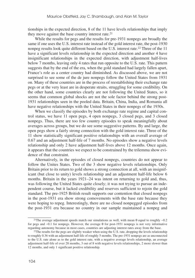
tionships in the expected direction, 8 of the 11 have levels relationships that implythey move against the base country interest rate.21
While the results for pegs and the results for pre-1931 nonpegs are broadly thesame if one uses the U.S. interest rate instead of the gold interest rate, the post-1930nonpeg results look quite different based on the U.S. interest rate.22 Three of the 11have a significant levels relationship in the expected direction and another 4 haveinsignificant relationships in the expected direction, with adjustment half-livesbelow 7 months, leaving only 4 rates that run opposite to the U.S. rate. This patternsuggests that by the end of the era, when the gold standard had largely fallen apart,France’s role as a center country had diminished. As discussed above, we are notsurprised to see some of the de jure nonpegs follow the United States from 1931on. Many of these countries are in the process of reestablishing their exchange ratepegs or at the very least are in desperate straits, struggling for some credibility. Onthe other hand, some countries clearly are not following the United States, so itseems that common global shocks are not the sole factor behind the strong post-1931 relationships seen in the pooled data. Britain, China, India, and Romania allhave negative relationships with the United States in their nonpegs of the 1930s.
When we classify the episodes by both exchange rate regime and capital con-trol status, we have 11 open pegs, 4 open nonpegs, 3 closed pegs, and 3 closednonpegs. Thus, there are too few country episodes to speak meaningfully aboutaverages across groups, but we do see some suggestive patterns. By and large, theopen pegs show a fairly strong connection with the gold interest rate. Three of the11 show statistically significant positive relationships with an overall average of0.67 and an adjustment half-life of 7 months. No episodes show a negative levelsrelationship and only 2 have adjustment half-lives above 12 months. Once again,it appears that the countries we expect to be constrained by the trilemma show evi-dence of that constraint.
Alternatively, in the episodes of closed nonpegs, countries do not appear tofollow the Unites States. Two of the 3 show negative levels relationships. OnlyBritain prior to its return to gold shows a strong connection at all, with an insignif-icant (but close to unity) levels relationship and an adjustment half-life below 6months. Britain in the years 1921–24 was intent on returning to gold and, thus,was following the United States quite closely; it was not trying to pursue an inde-pendent course, but it lacked credibility and reserves sufficient to rejoin the goldstandard. The pre-1925 British result supports our contention that closed nonpegsin the post-1931 era show strong comovements with the base rate because theywere hoping to repeg. Interestingly, there are no closed nonpegged episodes fromthe post-1931 era because no country in our sample maintained a nonpeg and
Maurice Obstfeld, Jay C. Shambaugh, and Alan M. Taylor
104
21The average adjustment speeds match our simulations as well, with mean θ equal to roughly −0.2for pegs and −0.1 for nonpegs. However, the average θ for post-1931 nonpegs is not very informativeregarding autonomy because in most cases, countries are adjusting interest rates away from the base.
22The results for the pegs are slightly weaker when using the U.S. rate, dropping the levels relationshipto roughly 0.36 with an adjustment half-life of roughly 5 months. The pre-1931 nonpegs are as unconnectedto the U.S. rate alone as to the gold interest rate, with a negative average levels relationship, an averageadjustment half-life of over 28 months, 3 out of 8 with negative levels relationships, 2 more slower than12 months, and only 1 significant positive relationship.
closed capital markets for as long as three years (our criterion for consideration asa distinct “episode”). Countries either briefly returned to pegs to break up stringsof nonpegging, or repegged within 3 years of leaving gold.
The results for the closed pegs are fairly close to those for open pegs, suggest-ing that perhaps closing capital markets does not entirely insulate a country if itintends to maintain a peg for a considerable length of time. None of the 3 levels rela-tionships is significant, but they are all positive, and 2 are quite close to 1. Theadjustment half-lives are all estimated to be between 4 and 8 months. Our datacomprise only 3 examples, though, of countries that maintained closed pegs for anyextended period, so it is difficult to conclude much about them. The open nonpegsare split, with 2 (Britain, 1931–34 and Italy, 1922–27) showing insignificant nega-tive levels relationships; 1 (Sweden, 1931–34) showing an insignificant, slowlyadjusting, positive relationship; and 1, (India, 1931–34) showing a significantpositive relationship with an adjustment half-life of 1 month.23
A final point worth noting is that interest rates in France and the United Stateswere never that closely related. Both during France’s prepegging episode from 1922to 1926, and during its peg from 1928 to 1936, a negative levels relationship pre-vailed. Thus, one sees part of the great tension in the system as a whole during thisera: the 2 center countries with the bulk of the gold reserves were moving their inter-est rates independently, making it difficult for countries to follow a single base.
Summary
The 2 types of econometric analysis broadly support the predictions of the trilemma.The pooled analysis shows that short-run interest rate movements in the pegged coun-tries, especially when they have open capital markets, follow the base interest rate.The levels analysis shows that on average, it is the open pegs or de jure pegs that fol-low the base the most closely over time. Notably, many nonpegs seem to show con-siderable independence from the base interest rate at many points in the sample. Anumber of countries that are briefly floating do combine to generate a high averageresponse of closed nonpegs to the base rate during the Great Depression, but this islargely an anomaly in our sample and the result is not significant.
Thus, we see that “fear of floating” type of behavior, while present in some cases,was not at all universal in our sample period as a whole. Many nonpeg countries wereable to move their interest rates in ways quite distinct from the base country. On theother hand, in times of crisis, more floating rate countries may have chosen to followthe base in an attempt to repeg, may have been forced to follow the base or risk fur-ther speculative attack, or may simply have been following the base because of glob-ally synchronized responses to large common shocks.
The trilemma finds considerable empirical support in this era, and the empir-ics generate results that are numerically consistent with theoretical, model-based
MONETARY SOVEREIGNTY, EXCHANGE RATES, AND CAPITAL CONTROLS
105
23The patterns when the U.S. interest rate is the base are similar, with the open pegs showing similarresults episode by episode, though with a slightly lower average half-life (in particular, Austria, Hungary,and India are somewhat weaker against the U.S. interest rate than against the gold interest rate). In othergroups, Germany shows a weaker relationship to the dollar rate as compared with the gold interest rate.Sweden’s interest rate during its open nonpeg has a significant levels relationship with the dollar ratedespite its insignificant relationship with the gold interest rate.
simulations. The trilemma was a constraint on policy for countries that fixed theirexchange rate and maintained open capital markets. They lost much of their mon-etary autonomy compared with countries that adopted alternative regimes. Theresults also show why the architects of Bretton Woods were so concerned to cre-ate a system that would allow for some monetary autonomy notwithstanding sta-ble exchange rates. The fact that some floaters did not pursue autonomy (as theycould have), and instead managed interest rates with an eye toward returning to apeg, may have convinced contemporaries like Keynes and Nurkse that the poten-tial instability of floating rates was not effectively compensated by any meaning-ful policy freedom. That view, in turn, led to the Bretton Woods consensus in favorof fixed exchange rates coupled with capital account control.
V. Conclusion
Up until now, the empirical content of the trilemma and, hence, its practical rele-vance, have remained largely untested. Our work seeks to show that the trilemmais a central feature of the macroeconomic world we have lived in for a century ormore. Understood in a target-zone context, the real world content of the trilemmadoes deviate from the simplistic idea of full international interest rate equalization,but only in degree. It is true that this deviation confers a little independence on pol-icymakers even under hard gold standard rules (Bordo, 2003; Bordo and Flandreau,2003; and Bordo and MacDonald, 1997, 2003). But that independence is very lim-ited indeed, we would argue. Under open capital markets and pegged exchangerates, the half-lives of interest rate deviations can be counted in months, and inter-est rate pass-through is very strong whether before or after World War I, or eventoday. It is not clear that such meager room for maneuver can offer any significantscope for purposeful macroeconomic management, especially when compared tothe far slower adjustment and lower pass-through seen in floating or closed capital-market countries. Only a move to floating or the imposition of capital controls canfree monetary policy to pursue domestic aims, and in practice they seem to do so.
Spanning, as it does, a century or more of experience, our empirical work inthis and other papers highlights the enduring power of this principle. In this sense,we would argue that the trilemma is alive and well. As a working proposition, itmerits attention from a wide audience, if our work is found to be persuasive. As anarrative hook, historians and political scientists have often invoked or criticized itsapplicability, but with little empirical evidence to guide interpretation. Internationaleconomists will find an old familiar part of their toolkit now has been sharpened upby use in the field. Last, but not least, policymakers may better comprehend the truenature of the constraints under which they must operate in an open economy.
REFERENCES
Baxter, Marianne, and Alan C. Stockman, 1989, “Business Cycles and the Exchange Rate Regime:Some International Evidence,” Journal of Monetary Economics, Vol. 23 (May), pp. 377–400.
Bloomfield, Arthur I., 1959, Monetary Policy Under the International Gold Standard: 1880–1914 (New York: Federal Reserve Bank of New York).
Maurice Obstfeld, Jay C. Shambaugh, and Alan M. Taylor
106
Board of Governors of the Federal Reserve System, 1943, Banking and Monetary Statistics1914–1941 (Washington: Board of Governors of the Federal Reserve System).
Bordo, Michael D., 2003, “Exchange Rate Regime Choice in Historical Perspective,” NBERWorking Paper No. 9654 (Cambridge, Massachusetts: National Bureau of EconomicResearch).
———, and Marc Flandreau, 2003, “Core, Periphery, Exchange Rate Regimes, and Glob-alization,” in Globalization in Historical Perspective, edited by M. D. Bordo, A. M. Taylor,and J. G. Williamson (Chicago: University of Chicago Press).
Bordo, Michael D., and Ronald MacDonald, 1997, “Violations of the ‘Rules of the Game’ andthe Credibility of the Classical Gold Standard, 1880–1914,” NBER Working Paper No. 6115(Cambridge, Massachusetts: National Bureau of Economic Research).
———, 2003, “The Inter-War Gold Exchange Standard: Credibility and Monetary Indepen-dence,” Journal of International Money and Finance, Vol. 22, No. 1, pp. 1–33.
Eichengreen, Barry J., 1996, Globalizing Capital: A History of the International MonetarySystem (Princeton: Princeton University Press).
———, and Douglas A. Irwin, 1995, “Trade Blocs, Currency Blocs, and the Reorientation ofWorld Trade in the 1930s,” Journal of International Economics, Vol. 38 (February), pp. 1–24.
Elliott, Graham, Thomas J. Rothenberg, and James H. Stock, 1996, “Efficient Tests for anAutoregressive Unit Root,” Econometrica, Vol. 64 (July), pp. 813–36.
Flood, Robert P., and Peter M. Garber, 1991, “The Linkage Between Speculative Attacks andTarget Zone Models of Exchange Rates,” Quarterly Journal of Economics, Vol. 106(November), pp. 1367–72.
Flood, Robert P., and Andrew K. Rose, 1995, “Fixing Exchange Rates: A Virtual Quest forFundamentals,” Journal of Monetary Economics, Vol. 36 (August), pp. 3–37.
Froot, Kenneth A., and Maurice Obstfeld, 1991, “Stochastic Process Switching: Some SimpleSolutions,” Econometrica, Vol. 59 (January), pp. 241–50.
Frankel, Jeffrey A., Sergio L. Schmukler, and Luis Servén, 2002, “Global Transmission of InterestRates: Monetary Independence and Currency Regime,” NBER Working Paper No. 8828(Cambridge, Massachusetts: National Bureau of Economic Research).
Goschen, George J., 1861, The Theory of the Foreign Exchanges (London: Effingham Wilson).
James, Harold, 2001, The End of Globalization: Lessons from the Great Depression (Cambridge,Massachusetts: Harvard University Press).
Kindleberger, Charles P., 1986, The World in Depression, 1929–1939, revised and enlarged edi-tion (Berkeley and Los Angeles: University of California Press).
Krugman, Paul R., 1991, “Target Zones and Exchange Rate Dynamics,” Quarterly Journal ofEconomics, Vol. 106 (August), pp. 669–82.
Kwiatkowski, Dennis, Peter Phillips, Peter Schmidt, and Yongcheol Shin, 1992, “Testing the NullHypothesis of Stationarity Against the Alternative of a Unit Root: How Sure Are We ThatEconomic Time Series Have a Unit Root?” Journal of Econometrics, Vol. 54, pp. 159–78.
League of Nations, 1930, Legislation on Gold (Geneva: League of Nations).
———, 1938, Monetary Review 1937/8 (Geneva: League of Nations).
———, Statistical Yearbooks, various editions.
Lindsey, Brink, 2002, Against the Dead Hand: The Uncertain Struggle for Global Capitalism(New York: John Wiley & Sons).
Mouré, Kenneth, 2002, The Gold Standard Illusion: France, the Bank of France, and the Inter-national Gold Standard, 1914–39 (Oxford: Oxford University Press).
MONETARY SOVEREIGNTY, EXCHANGE RATES, AND CAPITAL CONTROLS
107
Neal, Larry, and Marc Weidenmier, 2003, “Crises in the Global Economy from Tulips to Today:Contagion and Consequences,” in Globalization in Historical Perspective, edited by M. D.Bordo, A. M. Taylor, and J. G. Williamson (Chicago: University of Chicago Press).
Ng, Serena, and Pierre Perron, 2001, “Lag Length Selection and the Construction of Unit RootTests with Good Size and Power,” Econometrica, Vol. 69 (November), pp. 1519–54.
Obstfeld, Maurice, Jay C. Shambaugh, and Alan M. Taylor, 2004, “The Trilemma in History:Tradeoffs Among Exchange Rates, Monetary Policies, and Capital Mobility,” NBER WorkingPaper No. 10396 (Cambridge, Massachusetts: National Bureau of Economic Research).
Obstfeld, Maurice, and Alan M. Taylor, 1998, “The Great Depression As a Watershed:International Capital Mobility over the Long Run,” in The Defining Moment: The GreatDepression and the American Economy in the Twentieth Century, edited by M. D. Bordo,C. D. Goldin, and E. N. White (Chicago: University of Chicago Press).
———, 2003, “Sovereign Risk, Credibility, and the Gold Standard: 1870–1913 versus1925–31,” Economic Journal, Vol. 113 (April), pp. 1–35.
———, 2004, Global Capital Markets: Integration, Crisis, and Growth (Cambridge, England:Cambridge University Press).
Pesaran, M. Hashem, Yongcheol Shin, and Richard J. Smith, 2001, “Bounds Testing Approachesto the Analysis of Level Relationships,” Journal of Applied Econometrics, Vol. 16 (May/June),pp. 289–326.
Polanyi, Karl, 1944, The Great Transformation (New York: Rinehart).
Reinhart, Carmen M., and Kenneth S. Rogoff, 2004, “The Modern History of ExchangeRate Arrangements: A Reinterpretation,” Quarterly Journal of Economics, Vol. 119, No. 1,pp. 1–48.
Romer, David, 2001, Advanced Macroeconomics, second edition (New York: McGraw-Hill).
Rose, Andrew K., 1996, “Explaining Exchange Rate Volatility: An Empirical Analysis of ‘TheHoly Trinity’ of Monetary Independence, Fixed Exchange Rates, and Capital Mobility,”Journal of International Money and Finance, Vol. 15, No. 6, pp. 925–45.
Scammell, W. M., 1965, “The Working of the Gold Standard,” Yorkshire Bulletin of Economicand Social Research, Vol. 12, pp. 32–45.
Shambaugh, Jay C., 2004, “The Effects of Fixed Exchange Rates on Monetary Policy,”Quarterly Journal of Economics, Vol. 119, No. 1, pp. 301–52.
Svensson, Lars E. O., 1991, “The Term Structure of Interest Rate Differentials in a Target Zone:Theory and Swedish Data,” Journal of Monetary Economics, Vol. 28 (August), pp. 87–116.
Temin, Peter, 1989, Lessons from the Great Depression (Cambridge, Massachusetts: MIT Press).
Tortella, Gabriel, 2003, “Democracy and Gold” (unpublished; Universidad de Alcalá).
Yergin, Daniel, and Joseph Stanislaw, 1998, The Commanding Heights: The Battle BetweenGovernment and the Marketplace That Is Remaking the Modern World (New York: Simon& Schuster).
Maurice Obstfeld, Jay C. Shambaugh, and Alan M. Taylor
108


![[SEED SOVEREIGNTY]](https://static.fdocuments.in/doc/165x107/61ef3b9df0fbc95ef6306cbb/seed-sovereignty.jpg)