Monetary Policy with Declining Deficits: Theoryand an Application to Recent Argentine Monetary

Policy∗

Rody Manuelli Juan I. VizcainoWashington University in St. Louisand Federal Reserve Bank of St. Louis

May 29, 2017

Abstract

We study the nature of the optimal monetary policy in a regime of “fiscaldominance”when the monetary authority – that can print money or issue in-terest earning debt– is required to finance an exogenous sequence of transfersto the Treasury. We show that the degree of commitment on the part of themonetary authority has a significant impact on the details of the optimal policy.We apply this model to the recent experience of Argentina and we find thatthe inflation rate experienced by Argentina during the first year of the mone-tary program is close to the predictions of the weakly time consistent solution.Moreover, consistent with both versions of the model, the Argentine centralbank has increased the ratio of interest earning debt to monetary base.JEL Codes: E4, E5, Money, Monetary Policy

∗We thank Steve Williamson and two anonymous referees for their comments. The usual dis-claimer applies. Manuelli acknowledges financial support from the ADEMU project (A DynamicEconomic and Monetary Union) funded by the European Union (Horizon 2020 Grant 649396).

1

1 Introduction

In January 2016 the newly elected government of Argentina announced a policy ofdecreasing government budget deficits. It also specified what fraction of the deficitwould have to be financed by the monetary authority. In the case of Argentina, thisis a significant amount. For the year 2016 the Argentinean central bank (BCRA)was required to transfer to the Treasury approximately 2% of GDP out of a totalgovernment deficit of 4.8% of GDP. In addition, the BCRA decided to increase themonetary base by close to another 2.5% to increase the stock of foreign reserves.The Argentinean monetary authority finds itself in one of the versions of the econ-

omy that Sargent and Wallace (1981) studied in the well know “Unpleasant Mone-tarist Arithmetic”paper, namely, the case in which the fiscal authority moves firstand the monetary authority passively accommodates the fiscal demands. However,the problem faced by the BCRA differs from the problem studied by Sargent andWallace in that the BCRA can issue interest earning debt. Thus, the choice of mon-etary policy faced by the BCRA boils down to the choice of the mix between debtand money with the understanding that the only tax that it can use to service thedebt is the inflation tax.1

In this paper we study the policies that a monetary authority that is faced withsuch a temporary fiscal dominance situation – temporary in the sense that it is re-quired to transfer a declining amount of resources to the fiscal authority– shouldpursue. In a very general sense this is an optimal taxation problem and, like mostproblems of this type, the answer depends on the mix of taxes available and the de-gree of commitment on the part of the policy makers. In this particular applicationthe only tax available is the inflation tax so that the problem boils down to the choiceof distortionary inflation taxes over time. One possibility is to allow the stocks ofmoney to be determined by the time path of the expenditures that the central bankmust finance. Another option is control the quantity of money in the economy byissuing interest-earning securities. This allows the central bank to choose a timing ofincreases in the money supply that need not be the same as the timing of transfers.We consider the case of a central bank that can issue its own interest earning

securities of a given maturity and that, in the language of Del Negro and Sims (2015),

1It is impossible to determine why if issuing bonds is part of the optimal policy, the fiscalauthority chooses to delegate this to the monetary authority. The first best optimal policy is onein which the mix of all taxes – including the inflation tax– is pinned down and the consolidatedgovernment budget constraint determines the evolution of the public debt. The analysis of theinstituional arrangements that gives rise to this situation is beyond the scope of this paper.

2

it “does not have fiscal support,” that is, it cannot assume that the Treasury willrecapitalize with genuine resources the bank if it incurs losses in its portfolio. Thus,the only option available to the central bank is to collect seigniorage to remain solvent.Unlike the Federal Reserve Bank, it is not uncommon for central banks to issueactively tradable interest earning bills of different maturities2. Moreover, in manycountries, they are held by both financial and non-financial institutions. Accordingto Gray and Pongsaparn (2015) at least one third of their sample of central banksissue their own interest earning securities with a median maturity of a month butwith individual maturities as high as five years.3

The second element of our study is the temporary nature of the expenditures thatthe central bank incurs. As with the case of the interest earning securities, there isno obvious analog of this situation in the U.S. as the Fed is not required to maketransfers to the Treasury. However, this possibility is common in emerging countriesas central bank financing is an important share of government revenue and the modelapplies to any temporary increase in spending. For example, it includes not only thesituation in which the central bank is required to make temporary transfers to theTreasury but also the case in which the central bank responds to a banking crises byincreasing its liabilities to recapitalize financial institutions.4

What is the optimal monetary policy (or, equivalently, optimal debt policy) for acentral bank in the situation that we described above and given the available instru-ments? It turns out that the answer depends on the degree of commitment on thepart of the monetary authority as well as on the details of the amount of resourcesthat the monetary authority has to transfer to the fiscal authority which, from nowon, we will label the deficit.To make progress understanding optimal policies we study a very simple economy

in which the path of deficits and macro aggregates are known. This is similar to theeconomy that Uribe (2016) studies except that we only investigate the role of centralbank financing of a given deficit.We view the deficit as decreasing over time and eventually reaching zero. If the

monetary authority can precommit to any policy, then a relatively standard optimal

2The Federal Reserve Bank also issues a bill-like security since reserves earn interest. However,these securities are like callable bonds since the holders can turn them into money on demand.

3Nyawata (2012) Table 2 includes data on maximal maturities. In some cases, the upper bound isvery long. Thailand’s central bank can issue 20 year bonds while the Armenian monetary authoritycan issue 15 year bonds.

4Gray and Pongsaparn (2015) cite the case of the central bank of Chile that in the early 1980sissued a large amount of debt to sterilize increases in the money supply associated with bail outs ofdomestic banks. Stella and Lonnberg (2008) provide other examples.

3

taxation argument, as described in Uribe (2016), implies that the central bank shoulduse a mixture of monetary injections and debt to finance the required transfers. Thebasic idea is to smooth tax distortions – in this case the distortions associated withthe inflation tax– and to use interest earning debt to finance the difference betweenthe declining transfers and the revenue from the inflation tax. This is an extensionof the tax smoothing argument in Barro (1979) and the principles of financing ofgovernment spending in Lucas and Stokey (1983). The optimal policy is such thateven after the central bank is no longer required to finance a deficit it chooses toinflate so that it can service the existing debt and the present discounted value of therevenue from the inflation tax is equal to the present discounted value of the requiredtransfers.The assumption that the monetary authority is able to commit to positive inflation

in the presence of zero deficits is somewhat problematic since the central bank hasan incentive to implement a one time open market operation issuing non interest-earning money to buy the interesting-earning debt. In the absence of commitment,and depending on the stock of debt, such an open market operation can potentiallyresult in a jump in the price level but it allows the monetary authority to implementa zero inflation policy from then on.We will label policies that impose that inflation be zero when the deficit is zero

weakly time consistent policies. We show that weakly time consistent policies imposetight restrictions on the amount of debt that can be issued. In particular, they implythat the total value of nominal assets relative to output cannot exceed the ratio ofmoney to output under zero inflation. Our notion of weak time consistency amountsto requiring standard time consistency only when the fiscal situation is such thatthe monetary authority does not have to make any more transfers to the Treasury.As is well known in an economy with nominally denominated debt a time consistentpolicy is such that it engineers a large inflation as soon as possible to minimize thereal value of the debt. We do not find such an extreme version of time consistencya useful way of thinking about policy since it ignores other consequences of such anextreme policy. Thus, weak time consistency is a compromise that assumes that alleconomic participants – private sector and government alike– understand that thegovernment will be restricted about the policies that can implement in the future.We use this model to study the optimal monetary policy for Argentina, taking

as given the path of the deficit. We find that, consistent with both solutions, theArgentine monetary authority has increased the debt-money ratio over the first yearof the program. The key difference between the commitment and the weak time con-sistent solutions are the implications for the inflation rate. The commitment solution

4

estimates an average inflation of 2.6% while the weakly time consistent predicts avalue close to 25%. The recent Argentine experience – 33% inflation in the first yearof the program and a market expectation of 20% for the second year– appears to bemuch closer to the latter than to the former.The paper most closely related to ours – in addition to Uribe (2016)– is the

work by Diaz-Gimenez et. al. (2008) where it is also shown that time consistencylimits the ability of the monetary authority to implement optimal policies. The keydifference with our paper is that the path of deficits is not decreasing and that thereis coordination between the fiscal and monetary authorities which implies that taxesother than the inflation tax are used to finance the service of the debt. Martin (2013)has a thorough discussion of optimal policies in economies with different frictions. Herestricts himself to the case in which bonds have payoffs in real terms. In the contexta the New Keynesian models, Leeper et. al. (2016) discuss optimal monetary anddebt policy imposing time consistency. For a recent survey of monetary models andoptimal policies see Canzoneri (2011).There is a large literature that recognizes the fiscal dimension of monetary policy.

See, for example, Bassetto and Messer (2013), Berriel and Bhattarai (2009) and DelNegro and Sims (2015).

2 Model

We study the simplest economy that can be used to explore the role of lack of com-mitment. We take an off-the-shelf model similar to that used by Uribe (2016). Weassume that output, y, and government spending, g, are constant. This implies that,in equilibrium, consumption is constant as well. The fiscal authority picks a sequenceτ t of taxes and it demands from the monetary authority transfers xt = g − τ t. Weview xt as a decreasing function of time with the property that xt = 0 for all t ≥ T.It is convenient to separately describe the budget constraint for the monetary

authority and the rest of the government (which we will label the Treasury).5

• Treasury’s budget constraint:

BTt + Ptxt + Ptτ t = itB

Tt + Ptg,

where a dot over a variable indicates the time derivative. The income side ofthis constraint includes the sources of funds: bond issuance, BT

t , tax revenues,

5See Bassetto and Messer (2013) and Berriel and Bhattarai (2009) for example of anlyses thatdistinguish between the two budget constraints so as to keep track of monetary and fiscal interactions.

5

Ptτ t and transfer from the monetary authority, Ptxt. The expenditure side isthe sum of interest payments, itBT

t , and government purchases, Ptg.

• Monetary authority’s budget constraint:

Mt + BMt = itB

Mt + Ptxt.

The expenditure side of the central bank’budget constraint includes transferto the Treasury, Ptxt and interest payments on the debt it has issued, itBM

t .The only sources of funds are increases in the money supply, Mt, – defined asthe monetary base: currency in circulation plus non-interest earnings reserves–and interest earning debt, BM

t .

• The notation makes it clear that in the economy under study there is interestearning debt issued by the Treasury – which we denote by BT

t which has to bedistinguished from central bank issued debt, BM

t , since the latter is backed onlyby future increases in the real value of the money stock (seigniorage) as, in theeconomy that we study, we restrict Ptxt to be non-negative.

• Putting together these two budget constraints we arrive at the consolidatedbudgetary restriction for the government given by

Mt + BTt + BM

t + Ptτ t = it(BTt +BM

t ) + Ptg.

Given our focus in this paper – the optimal choice by the monetary authorityhow to finance the transfer Ptxt– this consolidated budget constraint plays aminor role

We assume that there is a representative dynasty that has preferences over con-sumption and real money balances given by

U =

∫ ∞0

e−ρt [u(ct) + v(mt)] dt,

where ct is consumption at time t and mt = Mt/Pt is real money balances6. Thefunctions u and v are assumed strictly concave and twice continuously differentiable.The private sector budget constraint is given by

Mt + BTt + BM

t = it(BTt +BM

t ) + Pty − Ptc− Ptτ t.6Effectively we are consolidating households and the non-governmental private sector. Thus, we

view mt as the real value of the monetary base and this includes the portion held by commercialbanks.

6

On the income side the representative dynasty earns interest at the nominal rate it onits holdings of treasury-issued debt, BT

t , as well as the stock of monetary authority-issued debt, BM

t . In addition, the representative agent earns income, spends resourcespurchasing consumption and pays taxes (if τ t < 0, the consumer receives a transfer).In what follows the key relationship is one between real money balances, consump-

tion and the nominal interest rate. It can be shown that the representative agent’sdemand for real money balances satisfies

v′(mt)

u′(ct)= it, (1)

where

mt =Mt

Pt

We assume that output is fixed and that government spending is constant. Thisimplies that private consumption is constant and, hence, that the real interest rate isequal to the discount factor. In equilibrium, the interest rate is

it = ρ+ πt

which is the standard Fisherian result. The monetary authority understands thetradeoffbetween inflation and real money balances as captured by equation (1) whichcan be more conveniently written as

v′(mt)

u′(c)= ρ+ πt. (2)

As mentioned before, the budget constraint of the monetary authority (not the con-solidated government budget constraint) is given by

Mt + BMt = itB

Mt + Ptxt,

which in real terms ismt + bMt = ρbMt + xt − πtmt,

where

bMt =BMt

Pt,

and seigniorage isst = mt + πtmt.

7

3 Optimal Monetary Policy

3.1 Optimal Policy Under Full Commitment

In this section we study the optimal monetary policy without imposing any restric-tions on the monetary authority other than those required to satisfy the budgetconstraint in equilibrium. Since output (and consumption) are fixed the optimalmonetary policy is the solution to the following problem

maxbMt ,mt

∫ ∞0

e−ρtv(mt)dt, (3)

subject to

mt + bMt = ρbMt + xt −(v′(mt)

u′(c)− ρ)mt, (4)

and the appropriate transversality condition. The optimal monetary policy (see Uribe(2016)) is summarized in the following result.

Proposition 1 (Optimal Policy Under Commitment [Uribe (2016)]) The op-timal policy is characterized by a constant level of real money balances, m, and aconstant inflation rate, π given by

π =v′(m)

u′(c)− ρ,

where m is chosen so that∫ ∞0

e−ρt[v′(m)

u′(c)m− xt

]dt = bM0 + m0.

and a debt policy given by

bMt = eρt(∫ t

0

e−ρs[xs −

(v′(m)

u′(c)− ρ)m

]ds+ bM0 + m0 −m

).

Proof. (See the Appendix)Under the optimal policy with commitment inflation is constant, and the stock of

debt initially increases and then decreases and it converges to zero as t→∞.

8

3.2 Weakly Time Consistent Optimal Policy

The optimal policy with commitment is such that after time T, the inflation taxis used to finance repayment of principal and interest on the debt issued by themonetary authority. This policy is not weakly time consistent. To see this considerwhat happens at time T. Let the stock of money at that time be denotedMT and thestock of bonds (in nominal terms) is BM

T . The problem faced by the central bank isto choose monetary policy to solve the continuation problem. Formally, the problemis

maxbMt ,mt

∫ ∞T

e−ρ(t−T )v(mt)dt,

subject to equation (4) which is

mt + bMt = ρbMt + xt −(v′(mt)

u′(c)− ρ)mt.

and subject to a given initial amount of total liabilities of the central bank, MT +BT .

Proposition 2 (Optimal Policy After Time T ) Assume that the central bank can-not issue negative debt, then the optimal monetary policy engineers an open marketoperation so that the resulting stocks of money and bonds are

M′

T = MT +BT ,

and the price level is

PT =M′T

m∗

and m∗ is such that the optimal inflation rate is zero, that is,

v′(m∗)

u′(c)= ρ

Proof. (See the Appendix)When the central bank is not required to finance any more deficits, there is no

longer any optimal taxation argument that requires any smoothing of distortions overtime and the economy reverts to the (constrained) first best. The optimal monetarypolicy solves a finite horizon version of the previous problem with the additionalterminal condition that the stock of central bank liabilities at time T must be equalto the level of real money balances under zero inflation. This condition amounts to

9

a restriction that the price level cannot jump at time T. This is one of the principlesof “honest government”as defined by Auernheimer (1974)The problem faced by the monetary authority is given by

maxbMt ,mt

∫ T

0

e−ρtv(mt)dt,

subject to

bMt = ρbMt + xt −(v′(mt)

u′(c)− ρ)mt,

and subject tomT + bMT = m∗.

Proposition 3 (Optimal Policy until T) The optimal policy is such that real moneybalances are constant and they satisfy

v′(m)m

u′(c)=

ρ

1− e−ρT

[(m0 + bM0 ) +

∫ T

0

e−ρtxtdt− e−ρTm∗]

Proof. (See the Appendix)Let Rt be the ratio of interest earnings bonds to real money balances. Thus,

Rt =bMtmt

.

Given that the optimal level of real money balances is m it follows that

Rt =eρt[(m0 + bM0 ) +

∫ t0e−ρs

(xs −

(v′(m)u′(c)

)m)ds]

m.

Since we are interested in the case in which deficits are declining, then the term(xs −

(v′(m)

u′(c)

)m

)is initially positive and it turns negative as t→ T. Thus, Rt is initially increasing andthen decreasing.Inflation is given by

π =

(v′(m)

u′(c)− ρ)

which is decreasing in real money balances.The key implication of the weak time consistency requirement is that the value

of the stock of liabilities of the monetary authority cannot exceed the level of thedemand for money under zero inflation.

10

4 Argentine Monetary Policy Through the Lens ofthe Model

In this section we briefly describe the recent monetary policy followed by the Argentinecentral bank, calibrate the model and study the implications under both commitmentand weak time consistency for the Argentine experience.

4.1 Recent Argentine Monetary Policy

The Institutional Framework The Argentine Central Bank’s charter specifiesthat its mission is “to promote, within its competencies and in agreement with thepolicy framework set forth by the national government, monetary stability, financialstability, employment and economic development in a framework of social fairness”(emphasis added).7 The board – including the president and vice-presidents– isappointed by the Executive branch with Senate agreement and it can be removed bythe Executive if a special commission of Congress agrees. In practice, it has not beendiffi cult for the Executive to replace the authorities of the central bank and that, forpractical purposes the Argentine central bank is not independent.8

The BCRA issues interest earning securities – as of this writing the only typeis denominated Lebacs– with a maturity that ranged from 28 to 273 days. Thesecentral bank bills and repos are used to conduct open market operations to regulatethe quantity of money. The BCRA also operates a discount window and manages thereserves of foreign currency.When the Argentine monetary authority transfers resources to the Treasury it

increases the liability side of its balance sheet by the amount of the transfers (anincrease in the monetary base) and, simultaneously, it increases the asset side byviewing the transfer as a loan labeled “Transitory Advances.”According to currentlegislation these “Transitory Advances”are capped at the max of 12% of the monetarybase or 10% of the annual government revenue. These loans have a duration of a

7The original in Spanish is “El banco tiene por finalidad promover, en la medida de sus facultadesy en el marco de las políticas establecidas por el gobierno nacional, la estabilidad monetaria, laestabilidad financiera, el empleo y el desarrollo económico con equidad social”.

8Even though by statute the president’s mandate lasts six years, the median duration of amandate over the last 30 years has been less than 9 months. It has been standard for incomingTreasury ministers to “choose” their own BCRA president. In many cases in which the BCRApresident’s and the Treasury’s positions do not agree the conflict is solved by the removal of theauthorities of the BCRA. For example, in 2012 the president was removed after he refused to useinternational reserves to honor debts.

11

year but continuous increases in the monetary base allow for indefinite renewals andincreases in the stock. In fact, these are never repaid.9 Since the BCRA has theability to issue its own interest earning debt it can conduct an open market operationin this security – conduct an auction– to absorb some or all of the increase in themoney supply.To illustrate the mechanism consider the following example: Suppose that the

BCRA wants to make a one time transfer to the treasury in the amount Z. Thiscreates an increase in the liability side of its balance sheet (an increase in the monetarybase) equal to Z. On the asset side the Transitory Advances account is increased byZ. If the central bank does not want to change the money supply this would be theend of the story.Consider now the case in which the central bank – for whatever reason– decides

that the monetary base should be only Z/2. Then, to absorb liquidity it auctionsoff interest earning securities in the amount Z/2. After a period – say, a year– thecentral bank increases the money supply to pay off the interest earning bills. Thus,after one period the money supply (and the liabilities of the central bank) equalZ + (Z/2)× i. On the asset side it is standard for the central bank to give the rest ofthe government a new loan in the amount Z. Thus, the Transitory Advances accountstill has a balance equal to Z. Since the BCRA has funded this “investment”in a zerointerest government loan with a mix of money (that pays no interest) and central bankbills (that earn a positive interest) the result is an operational loss. This reduces bankcapital and has to be compensated somehow. The details of how this is done varyacross the world. In some cases central banks simply “activate losses.”In other casesthe Treasury issues a non-negotiable zero interest long duration (e.g. over 50 years)bond that is used to recapitalize the bank.10 In the case of Argentina, the BCRAalso has foreign exchange reserves among its assets and it revalues them accordingto standard accounting practices. This creates a paper profit that has suffi ced tocompensate for the losses on the BCRA’s investment portfolio.

Recent Developments Even though a discussion of the monetary policy of Ar-gentina in beyond the scope of this paper, it is useful document the magnitude of the

9The law allows for doubling of the limits when economic conditions warrant such a change.This flexibility has been used in the recent past.

10For example, the government of Honduras transferred a bond that, in nominal terms, increasedthe capital of the central bank by 1.1% of GDP in 1997. However, Stella and Lonnberg (2008)estimate that the market value of that bond was 0.0006% of GDP.

12

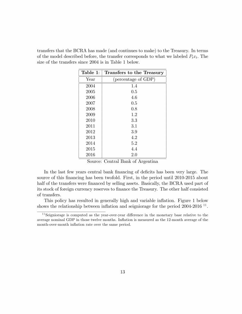
transfers that the BCRA has made (and continues to make) to the Treasury. In termsof the model described before, the transfer corresponds to what we labeled Ptxt. Thesize of the transfers since 2004 is in Table 1 below.

Table 1: Transfers to the TreasuryYear (percentage of GDP)2004 1.42005 0.52006 4.62007 0.52008 0.82009 1.22010 3.32011 3.12012 3.92013 4.22014 5.22015 4.42016 2.0Source: Central Bank of Argentina

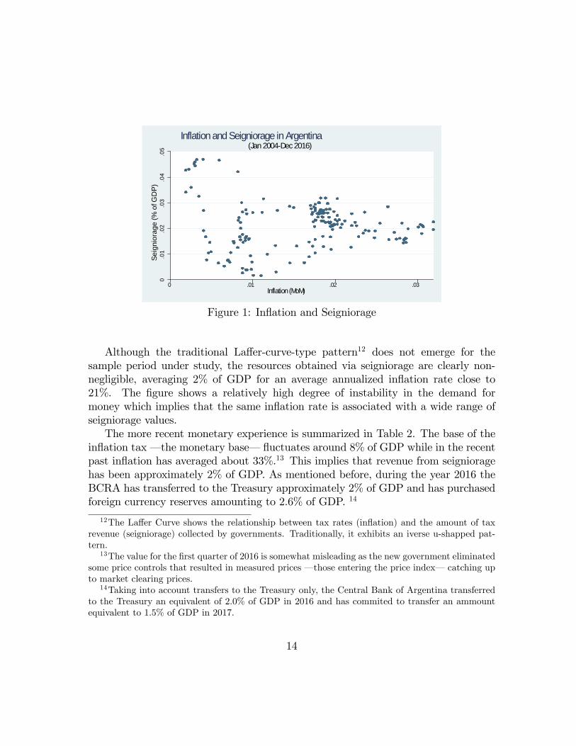
In the last few years central bank financing of deficits has been very large. Thesource of this financing has been twofold. First, in the period until 2010-2015 abouthalf of the transfers were financed by selling assets. Basically, the BCRA used part ofits stock of foreign currency reserves to finance the Treasury. The other half consistedof transfers.This policy has resulted in generally high and variable inflation. Figure 1 below

shows the relationship between inflation and seigniorage for the period 2004-2016 11.

11Seigniorage is computed as the year-over-year difference in the monetary base relative to theaverage nominal GDP in those twelve months. Inflation is measured as the 12-month average of themonth-over-month inflation rate over the same period.

13

0.0

1.0

2.0

3.0

4.0

5Se

igni

orag

e (%

 of G

DP)

0 .01 .02 .03Inflation (MoM)

(Jan 2004­Dec 2016)Inflation and Seigniorage in Argentina

Figure 1: Inflation and Seigniorage

Although the traditional Laffer-curve-type pattern12 does not emerge for thesample period under study, the resources obtained via seigniorage are clearly non-negligible, averaging 2% of GDP for an average annualized inflation rate close to21%. The figure shows a relatively high degree of instability in the demand formoney which implies that the same inflation rate is associated with a wide range ofseigniorage values.The more recent monetary experience is summarized in Table 2. The base of the

inflation tax – the monetary base– fluctuates around 8% of GDP while in the recentpast inflation has averaged about 33%.13 This implies that revenue from seignioragehas been approximately 2% of GDP. As mentioned before, during the year 2016 theBCRA has transferred to the Treasury approximately 2% of GDP and has purchasedforeign currency reserves amounting to 2.6% of GDP. 14

12The Laffer Curve shows the relationship between tax rates (inflation) and the amount of taxrevenue (seigniorage) collected by governments. Traditionally, it exhibits an iverse u-shapped pat-tern.

13The value for the first quarter of 2016 is somewhat misleading as the new government eliminatedsome price controls that resulted in measured prices – those entering the price index– catching upto market clearing prices.

14Taking into account transfers to the Treasury only, the Central Bank of Argentina transferredto the Treasury an equivalent of 2.0% of GDP in 2016 and has commited to transfer an ammountequivalent to 1.5% of GDP in 2017.

14

Table 2: Money and InflationPeriod 2015 2016Concept I II III IV I II III IVM/Y .09 .08 .09 .09 .08 .07 .08 .08B/M .56 .85 .54 .47 .67 .79 .82 .89Inflation .25 .27 .27 .34 .57 .31 .24 .20

Over the last year, the BCRA has been increasingly relying on interest earningdebt as an alternative to outright increases in the monetary base. Table 1 shows thatthere has been an increase in the ratio of central bank debt to money over the lasttwo years, and, in particular, since the beginning of the new monetary program in2016. During this last period the ratio of interest earning debt to the monetary basehas increased from 67% to almost 90%.We now develop a quantitative version of the model that is suitable to studying

optimal monetary policy in the context of the Argentine situation.

4.2 Theoretical Restrictions

We assume that

v(m) =(my)1−γ

1− γ z, u(c) =(cy + αy)1−γ

1− γ ,

where m is money demand relative to output, and c is the ratio of consumption-to-output, while α is a preference shifter that captures minimal levels of consumption.15

Following Lucas and Nicolini (2013), we take that the relevant concept of transactionsdemand for money is M1.The demand for money, m , satisfies

m = (c+ α) (zi)−1/γ .

This specification implies that seigniorage is given by

s(m) =

[z

(m1

c+ α

)−γ− r]m0,

15We experimented with a formulation that has a minimum level of money balances given byv(m) = (my+υy)1−γ

1−γ z but the estimate of υ was not significant.

15

where m0 is the monetary base (the base of the inflation tax). If the ratio of m1/m0

is denoted 1 + ζ then define

K ≡ z

(1 + ζ

c+ α

)−γ.

With this notation seigniorage is

s(m) =[K (m)−γ − r

]m

where, from now on, m denotes the stock of monetary base. Since we use seigniorageto estimate the relevant parameters it is clear that we can only identify K and notits individual components.For the time path of the deficit we assume the following functional form

xt =

{ψ0 − ψ1te−κ(T−t) t ≤ T0 t > T

.

Let,

x =

∫ T

0

e−ρtxtdt.

Given our choice of functional forms the optimal level of money balances in thecommitment case, mc, is the solution to

Km1−γc = ρ (w0 + x) . (5)

From Proposition 3 real money balances under weak time consistency, mw, satisfy

Km1−γw =

ρ

1− e−ρT(w0 + x− e−ρTm∗

)where m∗ is the solution to

K (m∗)−γ = ρ.

The level of real money balances under the weakly time consistent solution as

mw =

[ρ

K (1− e−ρT )

(w0 + x− e−ρT

(K

ρ

)1/γ)] 11−γ

(6)

and the implied inflation rate is

πw =K

mγw− ρ,

16

and the ratio of the two inflation rates is

πwπc

=

w0 + x− e−ρT(Kρ

)1/γ(1− e−ρT ) (w0 + x)

γγ−1

To summarize, the optimal level of real money balances in the commitment and weaktime consistent versions of the optimal monetary policy solve equations (5) and (6),respectively.From a qualitative perspective increases in the present value of the central bank

liabilities, w0+ x, not only increase the inflation rates in each of the two scenarios (asmore seigniorage is needed to finance the interest on the liabilities of the monetaryauthority) but also increases the gap between the inflation rates in the commitmentand weak time consistent solution. An increase in the demand for money, as measuredby an increase in K, decreases inflation in both regimes but more so in the weak timeconsistent case as it lifts up the demand for real money balances under zero inflation.16

Finally, increases in the time horizon reduce πw/πc.

4.3 Calibration

We use monthly data17 to estimate the following regression by Non-Linear LeastSquares (NLLS)

st =[Km−γt − r

]×mt + εt

where st is seigniorage in period t defined as the change in the monetary base relativeto the flow of output, mt is the monetary base, and εt is an error term. We assumethat r = ρ = 0.04.Since monetary policy in Argentina has been extremely variable with long pe-

riods in which financial institutions were forced to hold reserves in relatively largeproportions, we use monthly data for 2005-2015, a period with a relatively morestable monetary policy regime. One major disadvantage of using monthly data forArgentina (see Burdisso et. al. (2010)) is that seasonal fluctuations are large. In

16In May 2016 the BCRA announced an increase in the mandatory reserve requirements of thefinancial system that roughly corresponds to a 4% increase in the demand for money which, in ourcase corresponds to a 12% increase in K.

17Using monthly data requieres a monthly measure of private consumption and GDP. We con-struct these series by performing a cubic spline interpolation of their quarterly counterparts.

17

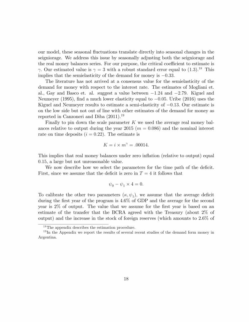
our model, these seasonal fluctuations translate directly into seasonal changes in theseigniorage. We address this issue by seasonally adjusting both the seigniorage andthe real money balances series. For our purpose, the critical coeffi cient to estimate isγ. Our estimated value is γ = 3 with a robust standard error equal to (1.3).18 Thisimplies that the semielasticity of the demand for money is −0.33.The literature has not arrived at a consensus value for the semielasticity of the

demand for money with respect to the interest rate. The estimates of Mogliani et.al., Gay and Basco et. al. suggest a value between −1.24 and −2.79. Kiguel andNeumeyer (1995), find a much lower elasticity equal to −0.05. Uribe (2016) uses theKiguel and Neumeyer results to estimate a semi-elasticity of −0.13. Our estimate ison the low side but not out of line with other estimates of the demand for money asreported in Canzoneri and Diba (2011).19

Finally to pin down the scale parameter K we used the average real money bal-ances relative to output during the year 2015 (m = 0.086) and the nominal interestrate on time deposits (i = 0.22). The estimate is

K = i×mγ = .00014.

This implies that real money balances under zero inflation (relative to output) equal0.15, a large but not unreasonable value.We now describe how we select the parameters for the time path of the deficit.

First, since we assume that the deficit is zero in T = 4 it follows that

ψ0 − ψ1 × 4 = 0.

To calibrate the other two parameters (κ, ψ1), we assume that the average deficitduring the first year of the program is 4.6% of GDP and the average for the secondyear is 2% of output. The value that we assume for the first year is based on anestimate of the transfer that the BCRA agreed with the Treasury (about 2% ofoutput) and the increase in the stock of foreign reserves (which amounts to 2.6% of

18The appendix describes the estimation procedure.19In the Appendix we report the results of several recent studies of the demand form money in

Argentina.

18

GDP).2021 Thus, κ, ψ1 solve

ψ1 ×(4 + (4− e−3κ)

2= .046

ψ1 ×(4− e−3κ + 4− 2e−2κ)

2= 0.02.

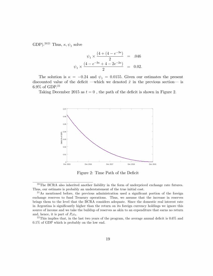
The solution is κ = −0.24 and ψ1 = 0.0155. Given our estimates the presentdiscounted value of the deficit – which we denoted x in the previous section– is6.9% of GDP.22

Taking December 2015 as t = 0 , the path of the deficit is shown in Figure 2.

Dec 2015 Dec 2016 Dec 2017 Dec 2018 Dec 20190

0.01

0.02

0.03

0.04

0.05

0.06

0.07

Defic

it (%

 of G

DP)

Figure 2: Time Path of the Deficit

20The BCRA also inherited another liability in the form of underpriced exchange rate futures.Thus, our estimate is probably an understatement of the true initial cost.

21As mentioned before, the previous administration used a significant portion of the foreignexchange reserves to fund Treasury operations. Thus, we assume that the increase in reservesbrings them to the level that the BCRA considers adequate. Since the domestic real interest ratein Argentina is significantly higher than the return on its foreign currency holdings we ignore thissource of income and we take the buildup of reserves as akin to an expenditure that earns no returnand, hence, it is part of Ptxt.

22This implies that, in the last two years of the program, the average annual deficit is 0.6% and0.1% of GDP which is probably on the low end.

19

As required by the theory, we impose that the initial value of the liabilities of thecentral bank equal to existing stock in December 2015 which was approximately 14%of output.

4.4 Implications of the Model and the Experience of Ar-gentina

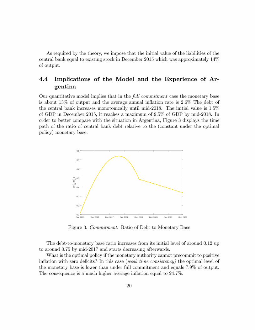
Our quantitative model implies that in the full commitment case the monetary baseis about 13% of output and the average annual inflation rate is 2.6% The debt ofthe central bank increases monotonically until mid-2018. The initial value is 1.5%of GDP in December 2015, it reaches a maximum of 9.5% of GDP by mid-2018. Inorder to better compare with the situation in Argentina, Figure 3 displays the timepath of the ratio of central bank debt relative to the (constant under the optimalpolicy) monetary base.

Dec 2015 Dec 2016 Dec 2017 Dec 2018 Dec 2019 Dec 2020 Dec 2021 Dec 20220.1

0.2

0.3

0.4

0.5

0.6

0.7

0.8

( bc M

t/m

c 0t)

Figure 3. Commitment: Ratio of Debt to Monetary Base

The debt-to-monetary base ratio increases from its initial level of around 0.12 upto around 0.75 by mid-2017 and starts decreasing afterwards.What is the optimal policy if the monetary authority cannot precommit to positive

inflation with zero deficits? In this case (weak time consistency) the optimal level ofthe monetary base is lower than under full commitment and equals 7.9% of output.The consequence is a much higher average inflation equal to 24.7%.

20

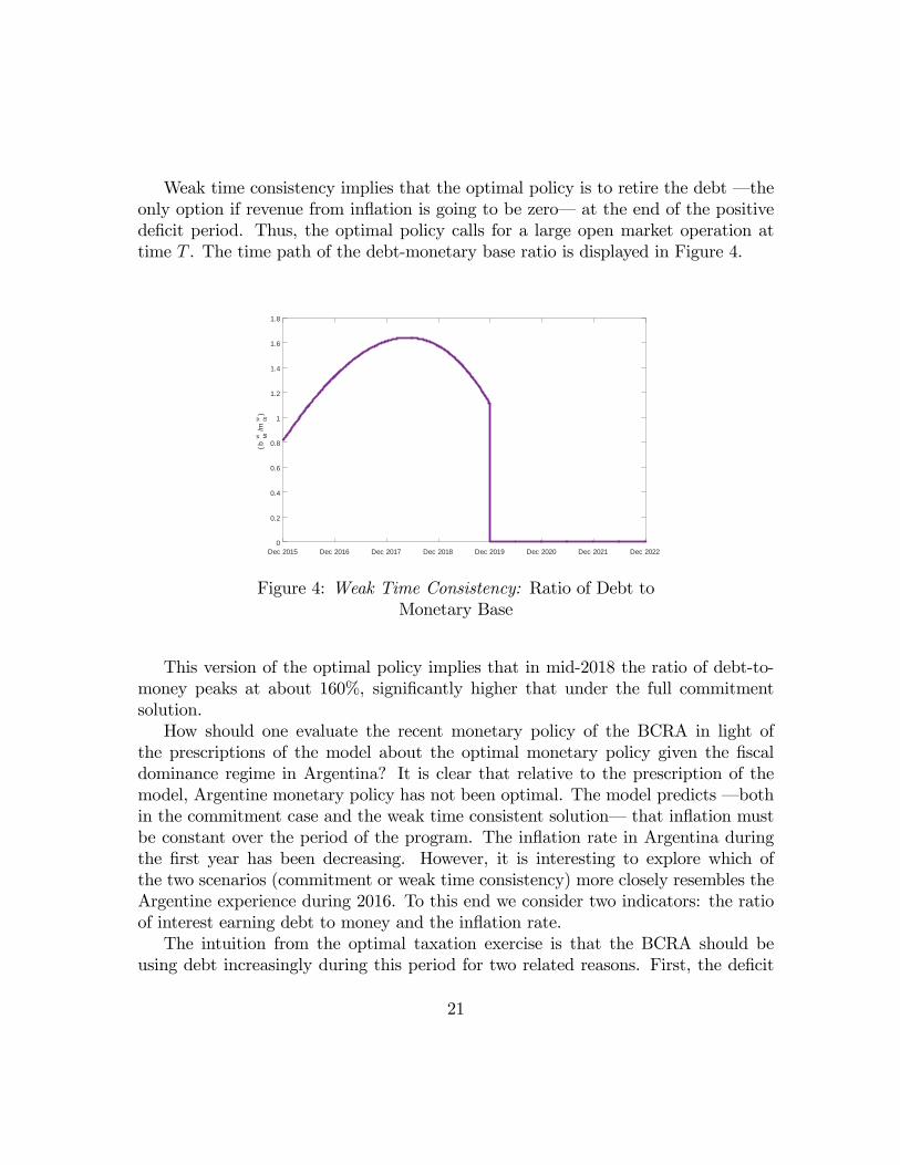
Weak time consistency implies that the optimal policy is to retire the debt – theonly option if revenue from inflation is going to be zero– at the end of the positivedeficit period. Thus, the optimal policy calls for a large open market operation attime T . The time path of the debt-monetary base ratio is displayed in Figure 4.

Dec 2015 Dec 2016 Dec 2017 Dec 2018 Dec 2019 Dec 2020 Dec 2021 Dec 20220

0.2

0.4

0.6

0.8

1

1.2

1.4

1.6

1.8

( bw M

t/m

w 0t)

Figure 4: Weak Time Consistency: Ratio of Debt toMonetary Base

This version of the optimal policy implies that in mid-2018 the ratio of debt-to-money peaks at about 160%, significantly higher that under the full commitmentsolution.How should one evaluate the recent monetary policy of the BCRA in light of

the prescriptions of the model about the optimal monetary policy given the fiscaldominance regime in Argentina? It is clear that relative to the prescription of themodel, Argentine monetary policy has not been optimal. The model predicts – bothin the commitment case and the weak time consistent solution– that inflation mustbe constant over the period of the program. The inflation rate in Argentina duringthe first year has been decreasing. However, it is interesting to explore which ofthe two scenarios (commitment or weak time consistency) more closely resembles theArgentine experience during 2016. To this end we consider two indicators: the ratioof interest earning debt to money and the inflation rate.The intuition from the optimal taxation exercise is that the BCRA should be

using debt increasingly during this period for two related reasons. First, the deficit

21

is viewed only as temporary. Second, because of the decision to increase the stockof foreign reserves during 2016, it is frontloaded. Both versions of the model –commitment and weak time consistent– prescribe that the debt-money ratio shouldhave increased during 2016. This is consistent with the evidence. The quantitativemodel implies that the debt-money ratio at the end of the first year of the programshould be between 47% (under commitment) and 133% (if the policy is weakly timeconsistent). The corresponding value for Argentina is 89%, roughly in the middle ofthe two estimates. Given the simplicity of the model it does not seem that using thisindicator can determine the degree of commitment implicit in the recent policy.The two versions of the model differ significantly in terms of their implications

for the inflation rate. Under commitment the inflation is estimated to be less than3% (average for the duration of the program) while the weak time consistent solutionestimates inflation to be much higher, close to 25%. The recent Argentine experienceseems to be much closer to the latter. As mentioned before, the inflation rate duringthe first year of the program was 33% and the market expectations for the secondyear are around 20%.23 Even if the BCRA succeeds in significantly lowering inflationduring the rest of the program it appears that the actual policy is better approximatedby the weak time consistent solution.In a recent paper, Uribe (2016) uses a similar model to analyze the Argentine

experience. He studies only the full commitment solution and includes in his analysisa much larger class of government debt as he is interested in how to finance theoverall deficit and not just the fraction that must be financed by the central bank.24

His estimates of the demand for money are different than ours as he assumes thatsemi-elasticity with respect to the interest rate is significantly lower than ours. Heconcludes that the inflation rate associated with the optimal policy is slightly below5% and the consolidated government’s debt-GDP ratio peaks above 40%.We view the more limited scope of our analysis that includes only the liabilities

of the central bank as a more appropriate use of the model. A comparison with theevidence suggests that this is the case.At the end of 2016 the total liabilities of the BCRA amounted to 16.2% of output.

Given our estimate of the present value of the deficit for the remaining three years ofthe program – x for the continuation is 2.6% of output– the weakly time consistentversion of the model implies that the average inflation rate will be close to 18%. There

23The latest available version of the BCRA’s Market Expectations Survey (REM) corresponds toJanuary 2017

24It does not appear that in his calculations Uribe takes into account the expenditures associatedwith the purchase of foreign reserves.

22

are two forces that influence the estimate of inflation. On the one hand, the presentdiscounted value of the deficit is substantially smaller (2.6% vs. 6.9%) reflecting thefrontloaded path of the deficit. This reduces required inflation. On the other hand,the stock of liabilities is higher (16.2% vs. 14%), and this requires a higher inflationrate. In a sense, our estimate is consistent with the view that inflation should bedecreasing in Argentina but – viewed as an average over the life of the program– itis higher than the offi cial forecasts.25

5 Concluding Comments

This note shows that the quantitative implications of the optimal monetary policyunder fiscal dominance depend on the assumed ability of the monetary authority tocommit. Under full commitment a standard optimal taxation argument shows thatthe monetary authority should issue both bonds and money. When the central bankcannot commit to a policy of positive inflation when the deficit is zero, then the abilityto smooth the distortion associated with the inflation tax is reduced and there is atight cap associated with the maximum amount of debt that the monetary authoritycan issue.In an example calibrated to capture the basic details of the recent monetary policy

of Argentina the model implies that the Argentine monetary authority has followeda policy that, to a first rough approximation, results in an inflation rate that is closeto that implied by the optimal policy under weak commitment. However, the actualpolicy deviates from the optimal in that the inflation rate is not constant.To what extent the issues that we discussed in this note apply to the U.S.? It is

important to note the differences in institutional setups between the type of centralbank that we analyzed – and, in particular, the Argentinean central bank– andthe Federal Reserve Bank. First, and most important, the Federal Reserve Bankis truly independent and, therefore, it does not have to agree to finance the rest ofthe government at a prespecified level.26 Second, the Fed does not issue longer terminterest earning securities and, hence, does not face the prospect of raising seigniorage

25The results of the model have to be taken as an approximation. There are at least two dimen-sions that can account for the difference in forecasts. First, the path of the deficit relative to GDPis best viewed as random. Second, the BCRA has indicated that the long run inflation rate is 5%rather than zero as we assumed.

26In the last few years the Fed has made substantial transfers to the Treasury as a result of theprofits associated with the management of its portfolio. However, these were not legally mandatedtransfers and it is unclear to us what would happen if the Fed starts incurring losses on its portfolio.

23

to service the debt.27

Are there lessons for the conduct of monetary policy in the U.S. that can be drawnfrom this exercise? The answer is a qualified yes. The Fed, just like the BCRA canissue a security – remunerated reserves– that can be used to drain liquidity fromthe system. Are there possible scenarios that the Fed could face that resemble theone analyzed in this paper? Ignoring some legal issues the Fed could find itself in asituation in which it has to transfer resources to the financial system, for exampleduring a banking crisis. In this case the Fed can choose to increase the money supplyin the form of non-interest bearing reserves to absorb part of the increase by payinginterest on some portion of the total reserves. This would come close to issuing interestearning securities to partially absorb excess liquidity. This type of arrangement isdifferent from the current situation in which all reserves receive the same return. Weview creating two types of reserves as the simplest way of creating a bond that, inthis example, would be held only by financial institutions.There is a sense in which the activities of the Fed since 2008 when it increased

its holdings of assets could fit in this framework. Ignoring for now the quality of theassets in the Fed’s portfolio (that were mostly high quality MBS and Treasuries) onecould argue that the ideas we discussed in this paper might apply to a central bankthat acquires private sector assets if, subsequently, the market value of those assetsdrops significantly. In that case the situation is analogous to the Fed making a onetime transfer to the private sector which is close to what we discussed.

27In the extreme case of losses in its asset portfolio the Fed can choose to pay no interest onreserves and, hence, cannot technically be required to increase the money supply in response todevelopments in its portfolio.

24

References

[1] Auernheimer, L., 1974, “The Honest Government’s Guide to the Revenue fromthe Creation of Money,”Journal of Political Economy, 82(3): 598-606.

[2] Barro, Robert, 1979, “On the Determination of the Public Debt,” Journal ofPolitical Economy, 87(6): 940-971.

[3] Basco, E., L. D’Amato and L. Garegnani, 2012, “The Information Value ofMoney for Forecasting Purposes: The Cases of Argentina and Chile,” BancoCentral de Argentina, working paper.

[4] Bassetto, M. and T. Messer, 2013, “Fiscal Consequences of Paying Interest onReserves,”Fiscal Studies, Vol. 34, No. 4, pp: 413-436.

[5] Berriel, T. and S. Bhattarai, 2009, “Monetary Policy and Central Bank BalanceSheet Concerns,”The B.E. Journal of Macroeconomics, Vol. 9, Issue 1, pp: 1-31

[6] Burdisso, T., Blanco, E., and Sardi, M., 2010 "Seasonal Adjustment and Lo-cal Calendar Effects in an Argentina’s Monetary Aggregate" Central Bank ofArgentina. Ensayos Económicos. June 2010.

[7] Canzoneri, M., R. and B. Diba, 2011, “The Interaction Between Monetaryand Fiscal Policy,” In Benjamin M. Friedman, and Michael Woodford, edi-tors: Handbook of Monetary Economics, Vol. 3B, The Netherlands: North-Holland, 2011, pp. 935-999.

[8] Cao, Q, 2015, “Optimal Fiscal andMonetary Policy with Collateral Constraints,”manuscript.

[9] Central Bank of Argentina, "Informe de Objetivos y Planes respecto del desar-rollo de la política monetaria, cambiaria, financiera y crediticia para el año 2017"Annual Targets and Programs Report of Central Bank of Argentina, 2017, pp:9-12.

[10] Del Negro, M. and C. Sims, 2015, “When Does a Central Bank’s Balance SheetRequire Fiscal Support?,”Federal Reserve Bank of New York, Staff Report No.701.

25

[11] Díaz-Giménez, J., Giovannetti, G., Marimon, R. and P. Teles, 2008, “NominalDebt as a Burden on Monetary Policy,”Review of Economic Dynamics, Volume11, Issue 3, pp: 493—514.

[12] Gay, A., 2005, “Money Demand in an Open Economy Framework: Argentina(1932-2002),”working paper, UNLP.

[13] Gray, S. and R. Pongsaparn, 2015, “Issuance of Central Bank Securities: Inter-national Experiences and Guidelines,”IMF working paper, wp/15/106.

[14] Kiguel, M. and P. Neumeyer, 1995, “Seignorage and Inflation: The Case ofArgentina,”Journal of Money Credit and Banking, Vol. 27, No. 3 , pp: 672-682.

[15] Leeper, E.,L. Campbell and L. Ding, 2016, “Optimal Time-Consistent Monetary,Fiscal and Debt Maturity Policy,”working paper.

[16] Lucas,R. Jr. and Nicolini, Juan, 2013. "On the stability of money demand," 2013Meeting Papers 353, Society for Economic Dynamics.

[17] Martin, F., 2013, “Government Policy in Monetary Economies,” InternationalEconomic Review, Volume 54, Issue 1, pp: 185—217.

[18] Mogliani, M., G. Urga and C.Winograd, 2009, “Monetary Disorder and FinancialRegimes. The Demand for Money in Argentina, 1900-2006,”working paper.

[19] Nyawata, O., 2012, “Treasury Bills and/or Central Bank Bills for AbsorbingSurplus Liquidity: The Main Considerations,”IMF working paper wp/12/40.

[20] Sargent, T. and N. Wallace, 1981, “Some Unpleasant Monetarist Arithmetic,”Federal Reserve Bank of Minneapolis Quarterly Review, Fall, pp:1-17.

[21] Stella, P. and A. Lonnberg, 2008, “Issues in Central Bank Finance and Indepen-dence,”IMF working paper, wp/08/37.

[22] Uribe, Martin, 2016, “Is the Monetarist Arithmetic Unpleasant?,”NBER work-ing paper 22866.

26

6 Appendix

6.1 Proofs

Proof of Proposition 1. The Hamiltonian of the problem is

HC = v(m) + λm

[ρbM + x−

(v′(m)

u′(c)− ρ)m− z

]+ λb(z).

where as a matter of notation we define

bM = z.

The first order conditions associated with the maximum problem are

λm = λb,

λm = ρλm − v′(m) + λm

[v′(m)

u′(c)− ρ− mv′′(m)

u′(c)

],

λb = ρλb − ρλm.

It follows that λb = λm = 0 and real money balances are given by

v′(m) = λm

[v′(m)

u′(c)− mv′′(m)

u′(c)

].

Thus, real money balances and the inflation rate are constant. The governmentbudget constraint implies that the real stock of central bank debt evolves accordingto

bMt = ρbMt + xt −(v′(m)

u′(c)− ρ)m,

and the solution that satisfies the transversality condition is such that

bMt = eρt(∫ t

0

e−ρs[xs −

(v′(m)

u′(c)− ρ)m

]ds+ (b0 +m0)−m

)In particular, the amount of debt issued by the monetary authority at t = 0 is∫ ∞

0

e−ρt[(

v′(m)

u′(c)− ρ)m− xt

]dt = bM0 + m0.

27

Proof of Proposition 2. The Hamiltonian for the central bank’s maximizationproblem is

HP = v(m) + λm

[ρbM + x−

(v′(m)

u′(c)− ρ)m− z

]+ λb (z) ,

which is similar to the one for the commitment case. The same argument then showsthat real money balances are constant and, under the policy that monetized the debt,inflation can be chosen so that∫ ∞

T

e−ρ(t−T )[(

v′(m)

u′(c)− ρ)m− xt

]dt = 0,

but since xt = 0 for all t ≥ T then m = m∗.Proof of Proposition 3. An argument similar to the previous proposition showsthat the optimal m is constant. Then central bank debt is given by

bMt +m = eρt[(m0 + bM0 ) +

∫ t

0

e−ρs(xs −

(v′(m)

u′(c)

)m

)ds

].

Imposing the terminal condition mT + bMT = m∗ we get the result.

6.2 Estimation

One issue with NLLS estimation is that, in some cases, estimates are very sensitiveto the initially chosen parameters. We provide to the estimation procedure an initialvalue for the money demand shifterK consistent with the average real money balancesrelative to output during the year 2015 (m = 0.086) and the nominal interest rateon time deposits (i = 0.22). We obtain K = 0.00014. In the case of γ, we provideas initialization point a set of values in the ranges suggested by the money demandestimation literature (from 0.5 to 20)In all cases we obtain K = 0.00018 (0.000585) and γ = 2.97 (1.32), where the

heteroskedasticity- and autocorrelation-consistent standard errors are reported be-tween parenthesis. Although the estimate for K is not statistically significant, a jointsignificance test suggests that the estimated coeffi cients are statistically significant atthe 1% level. For the quantitative simulation, and given that for K the confidenceinterval of the estimation suggests a wide range of possible values, we calibrate it insuch a way that it matches its average value for 2015.

28

6.3 Estimates of the Demand for Money

There are a number of estimates of the demand for money in Argentina. The differentestimates vary in terms of their coverage, the notion of money and how they handledynamic adjustment. These are the results from a cursory review of the literature:

1. Mogliani et. al. (2009?) find that in their estimation of the long run demandfor money allowing for structural breaks, real money balances – using M1 asthe notion of money– display a unit elasticity with respect to income while thesemi-elasticity with respect to the interest rate is -1.6.

2. Kiguel and Neumeyer (1995) define money as M1 and also estimate the demandfor money in different subperiods. They find that the coeffi cient of income isnot significantly different from zero and their estimates of the semi-elasticitywith respect to the interest rate range from -0.02 to -0.05.

3. Gay (2005) estimates the demand for money (does not say what he means bymoney) and he uses as his right hand side variable ln(it/(1 + it)). To turn hisestimate into a semielasticity requires taking a stand on the value of it. If Gay’sestimated coeffi cient is denoted β then the semielasticity is

β

(1 + it)it.

If we assume that it = 0.1 then the resulting semi-elasticity is (taking an averageof his estimates) -2.79, while if the interest rate is 20% (it = 0.2), the estimateis -1.24.

4. Basco et. al. (2012) estimate that the income elasticity of the demand formoney is slightly above 1 (not clear that one can reject that it is equal to one)and the interest semielasticity is -1.8.

It is not surprising that since Argentine monetary policy has been very unstableover the last half century with several episodes of hyperinflation it is not possible tofind robust estimates of the demand for money. In this paper we use some informationabout the semi-elasticity of the demand for money from the existing studies and wecomplement it with a very simple statistical model to obtain a reasonable parameter-ization of the relevant functions that allows us to make progress understanding therecent experience.

29

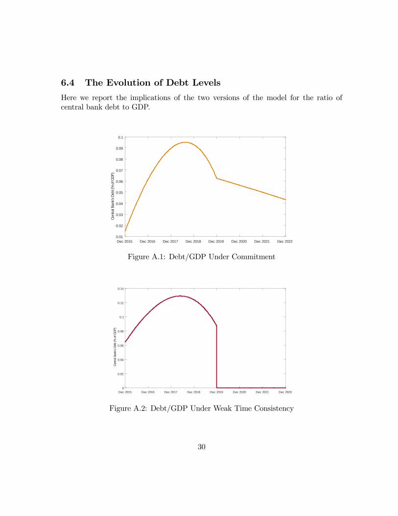
6.4 The Evolution of Debt Levels

Here we report the implications of the two versions of the model for the ratio ofcentral bank debt to GDP.

Dec 2015 Dec 2016 Dec 2017 Dec 2018 Dec 2019 Dec 2020 Dec 2021 Dec 20220.01

0.02

0.03

0.04

0.05

0.06

0.07

0.08

0.09

0.1

Cent

ral B

ank's

 Deb

t (%

 of G

DP)

Figure A.1: Debt/GDP Under Commitment

Dec 2015 Dec 2016 Dec 2017 Dec 2018 Dec 2019 Dec 2020 Dec 2021 Dec 20200

0.02

0.04

0.06

0.08

0.1

0.12

0.14

Cent

ral B

ank's

 Deb

t (%

 of G

DP)

Figure A.2: Debt/GDP Under Weak Time Consistency

30