Monetary policy transmission in China: A ... - uni … · Monetary policy transmission in China: A...
51
BOFIT Discussion Papers 9 • 2015 Michael Funke, Petar Mihaylovski and Haibin Zhu Monetary policy transmission in China: A DSGE model with parallel shadow banking and interest rate control Bank of Finland, BOFIT Institute for Economies in Transition
Transcript of Monetary policy transmission in China: A ... - uni … · Monetary policy transmission in China: A...

BOFIT Discussion Papers 9 • 2015
Michael Funke, Petar Mihaylovski and Haibin Zhu Monetary policy transmission in China: A DSGE model with parallel shadow banking and interest rate control
Bank of Finland, BOFIT Institute for Economies in Transition

BOFIT Discussion Papers Editor-in-Chief Laura Solanko BOFIT Discussion Papers 9/2015 9.3.2015 Michael Funke, Petar Mihaylovski and Haibin Zhu: Monetary policy trans-mission in China: A DSGE model with parallel shadow banking and interest rate control ISBN 978-952-323-033-0 ISSN 1456-5889 (online) This paper can be downloaded without charge from http://www.bof.fi/bofit. Suomen Pankki Helsinki 2015

BOFIT- Institute for Economies in Transition Bank of Finland
BOFIT Discussion Papers 9/ 2015
Contents
Abstract .................................................................................................................................. 4 1 Introduction ................................................................................................................... 5 2 Shadow banks and financial repression in China .......................................................... 7 3 Modelling China’s financial system with parallel shadow banking ............................ 11
3.1 Commercial banks and low-risk firms .................................................................. 13 3.2 Shadow banking and high-risk small and medium-sized firms ............................ 19 3.3 Optimism and shadow bank’s equity .................................................................... 22 3.4 Monetary policy .................................................................................................... 25 3.5 Interest rate liberalization scenarios ...................................................................... 27
4 Calibrated parameters .................................................................................................. 28 5 Model properties .......................................................................................................... 29
5.1 Impact of a contractionary monetary policy shock ............................................... 29 5.2 Impact of a positive technology shock to intermediate-good firm’s productivity 33 5.3 Expansionary window guidance shock ................................................................. 35 5.4 Shadow banking and welfare ................................................................................ 37
6 Concluding remarks ..................................................................................................... 39 References ........................................................................................................................... 41 Appendix A Rest of the model ......................................................................................... 43 Appendix B Model parameters ......................................................................................... 49
3

Michael Funke, Petar Mihaylovski and Haibin Zhu Monetary policy transmission in China: A DSGE model with parallel shadow banking and interest rate control
Michael Funke, Petar Mihaylovski and Haibin Zhu
Monetary policy transmission in China: A DSGE model with parallel shadow banking and interest rate control
Abstract The paper sheds light on the interplay between monetary policy, the commercial banking
sector and the shadow banking sector in mainland China by means of a nonlinear stochas-
tic general equilibrium (DSGE) model with occasionally binding constraints. In particular,
we analyze the impacts of interest rate liberalization on monetary policy transmission as
well as the dynamics of the parallel shadow banking sector. Comparison of various interest
rate liberalization scenarios reveals that monetary policy results in increased feed-through
to the lending and investment under complete liberalization. Furthermore, tighter regula-
tion of interest rates in the commercial banking sector in China leads to an increase in
loans provided by the shadow banking sector.
Keywords: DSGE model, monetary policy, financial market reform, shadow banking,
China
JEL: E32, E42, E52, E58
Michael Funke, Department of Economics, Hamburg University and CESifo, Munich, GERMANY. Email: [email protected]
Petar Mihaylovski, Department of Economics, Hamburg University, GERMANY. Email: [email protected]
Haibin Zhu, JP Morgan Chase Bank, HONG KONG. Email: [email protected] Acknowledgement We would like to thank Fabio Verona (Bank of Finland) for sharing his DYNARE code. We are grateful for the hospitality of the Hong Kong Institute for Monetary Research (HKIMR) and the Bank of Finland Institute for Economies in Transition (BOFIT) during the 2014–15 academic year. The views expressed herein are those of the authors and should not be attributed to the HKIMR or BOFIT.
4

BOFIT- Institute for Economies in Transition Bank of Finland
BOFIT Discussion Papers 9/ 2015
1 Introduction The Chinese financial system has undergone gradual refoms since the mid 1990s. In the
wake of the Asian crisis of 1997, the Chinese authorities recognized that structural reforms
and better regulation were necessary to tackle the growing systemic risks of the Chinese
financial system. At that time more than 20% of loans were nonperforming, which implied
potential losses in excess of banks’ net assets. The banking cleanup lasted more than a
decade and achieved considerable success. The bad debts have been replaced a decade later
by highly profitable and well-capitalized banks. A concomitant effect, however, has been a
policy of allowing large-scale interest rate distortions. This policy prevented banks from
collapsing. But China´s policy of financial repression, whose main feature is a regulated
interest rate system, forces households to endure artificially low interest rates on bank
deposits. Another direct consequence of the tight interest rate regulation is that access to
bank loans tends to be limited and uneven across borrowers. This has led to the emergence
of a shadow banking system as an important channel for alternative funding. The
superficial reason is that Chinese banks are not extending enough credit to small- and
medium-sized enterprises (SMEs), but are focusing instead on lending to established large
Chinese firms.
This distorted interest rate structure has discouraged marginal investment and is a
significant obstacle to sustaining China´s rapid economic growth. The global recession of
2008 – 2009 aggravated these difficulties in China´s financial system, as the government´s
huge stimulus package in response to the crisis emphasized bank loans rather than direct
government spending which entails a sizable risk of non-performing loans, and impaired
bank balance sheets in the future. In addition, new financing channels outside the well-
regulated banking system have subsequently developed and expanded further aggravating
the risk management challenges for monetary policy and regulators. Thus, the Chinese fi-
nancial system again stands at a cross-roads and requires a new round of reforms to ad-
dress the challenges that have accumulated over the past several years.1
1In line with this, the third plenum of the Chinese Communist Party in November 2013 has called for equal competition where firms must freely make resource allocation decisions considering market-based input prices. However, the Chinese State Council said the shifts would be carried out in an “orderly way” - usually a buzzword for moving slowly. Thus the Chinese authorities will most likely employ a piecemeal approach where those tools for which the impacts are well known are frequently used while others will be put on hold.
5

Michael Funke, Petar Mihaylovski and Haibin Zhu Monetary policy transmission in China: A DSGE model with parallel shadow banking and interest rate control
Against this background, our paper addresses the Chinese shadow bank issue and
contributes to the literature on modelling parallel shadow banks and interest rate control in
micro-founded dynamic stochastic general equilibrium (DSGE) frameworks. Few theoreti-
cal analyses exist to guide policymakers in this way. This paper is most closely related and
complementary to three recent papers modelling a shadow banking sector, but differs in
several respects. Verona et al. (2013) consider a financial accelerator DSGE model for the
US economy with investment banks investing in less risky projects while formal retail
banks provide funding to riskier firms. They are mainly concerned with the adverse effects
of shadow banking for boom-bust events caused by a level of interest rates that is too low
for too long. Meeks et al. (2014) are concerned about financial instability due to commer-
cial banks unloading risky loans to off-balance sheet shadow banks via securization. Maze-
lis (2014) has investigated the impact of monetary policy shocks on aggregate loan supply
in a DSGE framework with commercial banks and shadow banks. In contrast to Meeks et
al. (2014), Mazelis (2014) does not assume that shadow banks are funded by the commer-
cial banking sector; instead, shadow banks have to acquire deposits from the markets in
order to function as intermediaries. The funding market is modelled via search and match-
ing by shadow banks for available deposits of households. Our paper differs from the exist-
ing papers in a number of ways. None of the above papers focuses on the multifaceted in-
teractions between nonstandard monetary policy, the traditional banking sector and the
shadow banking sector in China. In our DSGE framework, in contrast, we analyze mone-
tary policy transmission with parallel shadow banking and different degrees of interest rate
control. This means, as a corollary, that we also investigate the impacts of financial liber-
alization and regulatory change in China on shadow banking.
The remainder of the paper is organized as follows. Section 2 provides a brief
overview of shadow banking activities in China: the products, the range of participants,
and the reasons behind their rapid increase. We devote section 3 to the careful construction
of a tractable DSGE model with a parallel shadow banking sector. Section 4 presents the
model calibration. Section 5 presents impulse response functions and model simulations
and analyze the main channels at work. Finally, Section 6 concludes. Omitted modelling
and calibration details are provided in two appendices. To economize on space, the com-
plete set of equilibrium conditions is available in an Online Appendix at BOFIT DP
website at http://www.suomenpankki.fi/bofit_en/tutkimus/tutkimusjulkaisut/dp/
Documents/2015/dp0915_app.pdf.
6

BOFIT- Institute for Economies in Transition Bank of Finland
BOFIT Discussion Papers 9/ 2015
2 Shadow banks and financial repression in China What is shadow banking? The definition of shadow banking is itself shadowy. According
to the Financial Stability Board (FSB), shadow banking is “credit intermediation involving
entities and activities outside the regulated banking system”. In other words, off balance
sheet shadow banking moves financial intermediation (fully or partially) outside of regular
banking and thus circumvents safeguards such as capital requirements, loan-loss provi-
sions, loan-to-deposit ratios, and well-established supervision and regulation. The FSB also
suggests a narrow definition of shadow banking as a “subset of non-bank credit interme-
diation where there are (i) developments that increase systemic risk (in particular matur-
ity/liquidity transformation, imperfect credit risk transfer, and/or leverage), and/or (ii) indi-
cations of regulatory arbitrage that is undermining the benefits of financial regulation.”2
The definition and the development of shadow banking are country-specific. In
China, shadow banking activity emerged in the wake of a “dual-track” reform strategy in
interest rate liberalization. As a background information, note that interest rates are heavily
regulated in China. In 2004, the central bank removed lower bound restrictions on deposit
rates and upper bound restrictions on lending rates, but maintained upper bound restric-
tions on deposit rates and lower bound restrictions on lending rates.
Figure 1 One-year benchmark deposit and lending rates in %: January 2008 – September 2014
Note: The green (red) line is the nominal benchmark lending (deposit) rate. Data source: CEIC and Bloomberg.
2 See FSB (2013) and Li (2013) for an overview of definitions used in the literature. FSB (2014) monitors financial stability risks using end-2013 data. The definition implies that shadow banking entities do not in-clude equity-based funds and venture capital companies, which do not make use of credit instruments in the financing process.
7

Michael Funke, Petar Mihaylovski and Haibin Zhu Monetary policy transmission in China: A DSGE model with parallel shadow banking and interest rate control
The PBoC has gradually eased interest rate controls in recent years. On the deposit rate
side, it introduced as a maximum a 10% premium above benchmark deposit rates in June
2012 and raised it further to 20% in November 2014. Despite this liberalization, the deposit
rate ceiling still appears to be binding, as deposit rates remain clustered at their upper
bound. On the lending rate side, People’s Bank of China (PBoC) raised the maximum dis-
count from the benchmark lending rate from 10% to 20% in June 2012, then to 30% in July
2012, and it finally removed lending rate control in July 2013. At end-2013, 24% of bank
loans offered were at discounts from the benchmark lending rates and 63% were at pre-
mium. Table 1 indicates that in practice there is no longer a strict enforcement mechanism.
The PBoC also controls bank credit through its administrative window guidance
policy on commercial bank lending. This quantity-based non-price instrument is an impor-
tant tool in the conduct of monetary policy and can be understood as gentle coersion
through formal statements or private discussions. Under this policy, the PBoC persuades
banks to lend according to the guideline. The guidance typically covers the level of loan
growth and sectors to which bank lending should be directed. Such window guidance has
been important in driving bank loan growth in recent years, which was 32% in 2009 and
20% in 2010 in support of the large stimulus package, and continued to decelerate after
2011 amid the central bank’s efforts to normalize monetary policy (loan growth was 13.6%
in 2014). Furthermore, since 2012 the bank regulator has restricted bank lending to local
government financing platforms and the real estate sector, and has encouraged bank lend-
ing to SMEs and to rural sectors.
China´s shadow banking initially emerged to support interest rate liberalization, a
“dual-track” reform strategy which aims to develop market-based deposit and lending rates
outside the banking system. For instance, wealth management products (WMP) are a result
of the search-for-yield effect and the endeavour to bypass regulation on maximum deposit
rates. WMPs are typically short term (usually less than 6 months) and marketed as high-
yield alternatives to bank deposits. Separately, trust loans are alternatives to bank loans, in
which a trust company invests client funds according to a pre-specified objective, purpose,
amount, maturity, and interest rates (which is not subject to interest rate control).
8

BOFIT- Institute for Economies in Transition Bank of Finland
BOFIT Discussion Papers 9/ 2015
Table 1 Share of commercial loans issued at different rates December 2007 – December 2014
Year Below benchmark At benchmark Above benchmark
December 2007 28.07 27.69 44.24
December 2008 25.56 30.13 44.31
December 2009 33.19 30.26 36.55
December 2010 27.80 29.16 43.04
December 2011 7.02 26.96 66.02
December 2012 14.16 26.10 59.74
December 2013 12.48 24.12 63.40
December 2014 13.10 19.64 67.26
Data source: CEIC and Bloomberg. The other, and perhaps more important, reason for the rapid growth in China's shadow
banking is regulatory arbitrage. This is a major reason for the rapid growth of shadow
banking in China since 2012, when the Chinese authorities started to counter inflation after
the large-scale stimulus program in response to the global financial crisis 2008–2010. Fur-
thermore, PBoC raised the bank reserve requirement ratios 12 times in 2010 and 2011 to a
record high of 21.5 percent for large institutions in June 2011. In response, WMP and
trusts driven by investors’ quest for higher yields formed a parallel lending channel to sup-
port those borrowers with limited access to bank loans. In a typical shadow banking credit
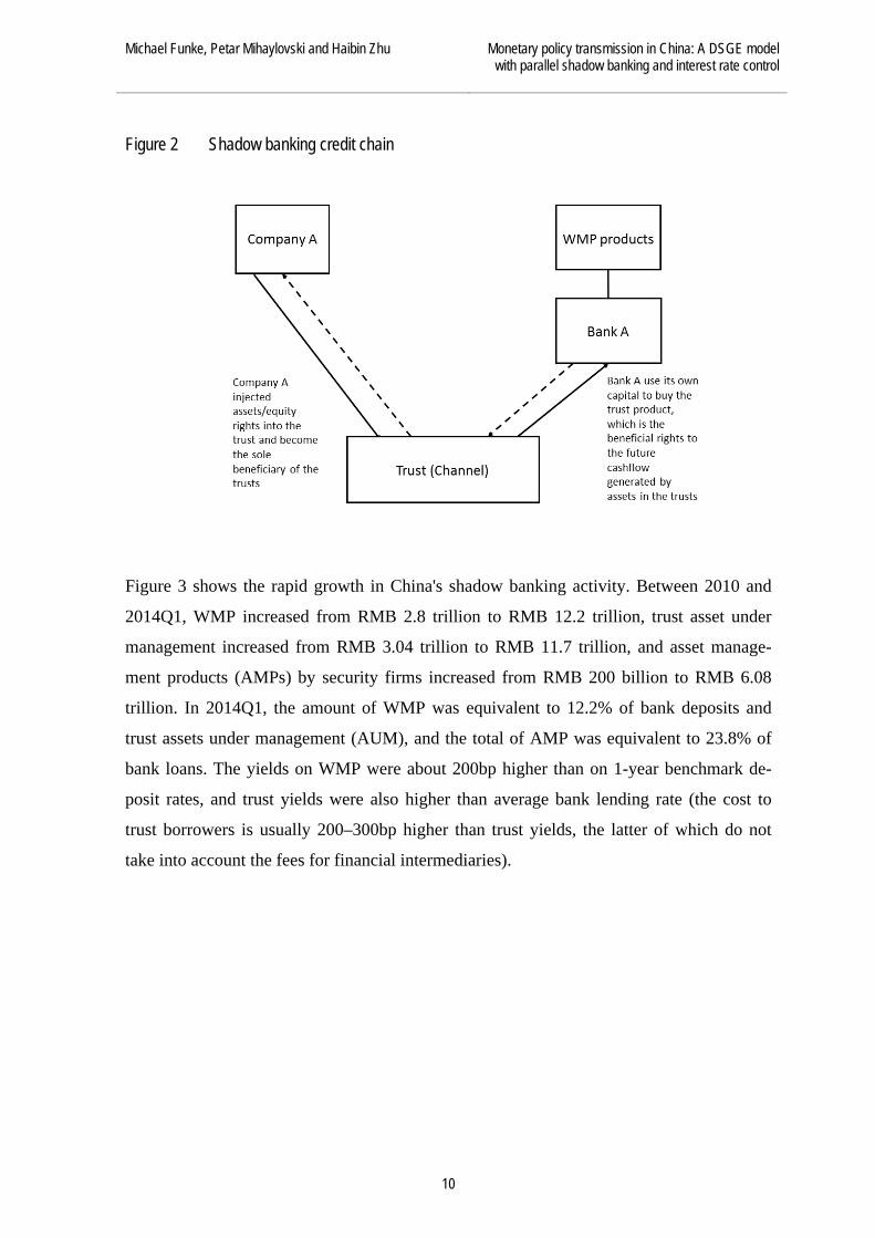
chain, a trust company received funds via WMPs and then lent to these borrowers (Figure
2). Because WMPs are banks’ off-balance sheet items and can offer attractive yields to in-
dividual investors, while trust companies do not face interest rate restrictions, loan quotas,
or loan-to-deposit ratio requirements, and are subject to lighter regulation, these parallel
lending channels have grown rapidly and support economic growth. In a nutshell, the
growth of the Chinese shadow banking system results in distortions in the formal financial
system as well as in elements of the monetary and regulatory policy framework.3
3The WMP vehicles enhance the tradability of credit portfolios, thereby allowing shadow banks to free up resources by selling loans. This in itself can give shadow banks greater scope for lending. See Altunbas et al. (2009).
9
Michael Funke, Petar Mihaylovski and Haibin Zhu Monetary policy transmission in China: A DSGE model with parallel shadow banking and interest rate control
Figure 2 Shadow banking credit chain
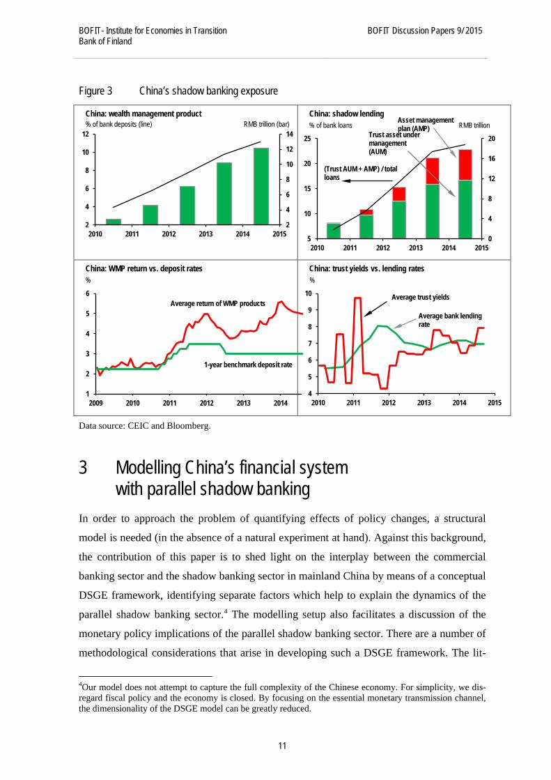
Figure 3 shows the rapid growth in China's shadow banking activity. Between 2010 and
2014Q1, WMP increased from RMB 2.8 trillion to RMB 12.2 trillion, trust asset under
management increased from RMB 3.04 trillion to RMB 11.7 trillion, and asset manage-
ment products (AMPs) by security firms increased from RMB 200 billion to RMB 6.08
trillion. In 2014Q1, the amount of WMP was equivalent to 12.2% of bank deposits and
trust assets under management (AUM), and the total of AMP was equivalent to 23.8% of
bank loans. The yields on WMP were about 200bp higher than on 1-year benchmark de-
posit rates, and trust yields were also higher than average bank lending rate (the cost to
trust borrowers is usually 200–300bp higher than trust yields, the latter of which do not
take into account the fees for financial intermediaries).
10
BOFIT- Institute for Economies in Transition Bank of Finland
BOFIT Discussion Papers 9/ 2015
Figure 3 China’s shadow banking exposure
Data source: CEIC and Bloomberg.
3 Modelling China’s financial system with parallel shadow banking
In order to approach the problem of quantifying effects of policy changes, a structural
model is needed (in the absence of a natural experiment at hand). Against this background,
the contribution of this paper is to shed light on the interplay between the commercial
banking sector and the shadow banking sector in mainland China by means of a conceptual
DSGE framework, identifying separate factors which help to explain the dynamics of the
parallel shadow banking sector.4 The modelling setup also facilitates a discussion of the
monetary policy implications of the parallel shadow banking sector. There are a number of
methodological considerations that arise in developing such a DSGE framework. The lit-
4Our model does not attempt to capture the full complexity of the Chinese economy. For simplicity, we dis-regard fiscal policy and the economy is closed. By focusing on the essential monetary transmission channel, the dimensionality of the DSGE model can be greatly reduced.
2
4
6
8
10
12
14
2
4
6
8
10
12
2010 2011 2012 2013 2014 2015
% of bank deposits (line) China: wealth management product
RMB trillion (bar)
0
4
8
12
16
20
5
10
15
20
25
2010 2011 2012 2013 2014 2015
% of bank loans China: shadow lending
RMB trillion
(Trust AUM + AMP) / total loans
Trust asset under management (AUM)
Asset management plan (AMP)
1
2
3
4
5
6
2009 2010 2011 2012 2013 2014
% China: WMP return vs. deposit rates
1-year benchmark deposit rate
Average return of WMP products
4
5
6
7
8
9
10
2010 2011 2012 2013 2014 2015
% China: trust yields vs. lending rates
Average trust yields
Average bank lending rate
11

Michael Funke, Petar Mihaylovski and Haibin Zhu Monetary policy transmission in China: A DSGE model with parallel shadow banking and interest rate control
erature has not yet presented an all-encompassing DSGE model appropriate for modelling
China’s shadow banking sector, but several elements have been developed, and we natu-
rally build on them. The papers by Chen et al. (2012) and Funke and Paetz (2012) develop
a nonlinear DSGE model that captures China’s nonstandard monetary policy toolkit. In this
paper we augment that framework with a shadow banking sector, along the lines of Verona
et al. (2013). The latter is a simplified version of the financial accelerator model proposed
by Christiano et al. (2010). We deliberately adopted a modelling approach that considers
only a simplified version of the interbank market. This choice has the virtue of keeping the
model simple without changing the nature of our modelling results. In simple terms, our
goal is to capture, for China, the interface between qualitative and quantitative monetary
policy versus shadow banking.5 A diagrammatic drawing of the main elements of the mod-
elling framework is given in Figure 4.
The modelling setup assumes homogeneity in the household sector and heteroge-
neity among banks and firms. Next we sketch the representation of the banking and firm
sectors. The model is populated by two types of banks: a commercial bank and a shadow
bank. China’s shadow banking activities typically involve direct lending to firms with un-
met demand for loans. The so-called “trusts” pool money from investors promising a state-
contingent return. There are two types of firms in the economy: Perceived low-risk large
private and state-owned firms (SOEs) and perceived high-risk SMEs. It is widely taken as
a fact that the Chinese government implicitly guarantees much, if not all, of SOEs’ debt.
Accordingly, the large and state-owned firms have access to cheap funding from the com-
mercial banking sector. In contrast, the SMEs fraught with risk find it difficult to borrow
from the formal banking sector. In addition, high-risk firms are not able to self-finance
their capital purchases and households cannot lend to SMEs directly. All this confers that
the SMEs interact with the shadow banking sector. Shadow banking finance typically car-
ries a higher interest rate than commercial bank finance.6 In what follows, superscripts se
and re stand for large private and state-owned firms and small and medium-sized firms,
5It is worth bearing in mind that we do not attempt to model the process of financial innovation and deregula-tion which lies behind the rapid expansion of the Chinese shadow banking sector. Instead, we focus upon the policy issues of nonstandard monetary policy tools, shadow banking activities and further interest rate liber-alization in China. 6The higher shadow banking lending rates are consistent with the Berlin and Mester (1999) model consider-ing the contracting relationship between a firm and a bank. The core feature of the model is the setting of lending rates subject to the liability structure of the bank.
12

BOFIT- Institute for Economies in Transition Bank of Finland
BOFIT Discussion Papers 9/ 2015
respectively. Finally, a non-standard Chinese monetary policy rule completes the model.
Next we describe the ingredients of the modelling environment in more detail.
Figure 4 Structure of the DSGE model
3.1 Commercial banks and low-risk firms To fix the modelling ideas and notation, we start with low-risk firms. Low-risk firms’ role
in this model is to purchase physical capital from capital producers and provide it to inter-
mediate-good firms. The timing of this process goes as follows. At the beginning of period
t the low-risk entrepreneur provides capital services to the intermediate-good firms. Capital
services are related to the stock of physical capital as 𝐾𝑡𝑠𝑒 = 𝑢𝑡𝑠𝑒𝐾�𝑡𝑠𝑒 where 𝑢𝑡𝑠𝑒 stands for
capital utilization. The latter faces an increasing and convex cost function of the form
(1) 𝑎(𝑢𝑡𝑠𝑒) = �̅�𝑘,𝑠𝑒
𝜎𝑎𝑠𝑒[exp(𝜎𝑎𝑠𝑒(𝑢𝑡𝑠𝑒 − 1)) − 1]
13

Michael Funke, Petar Mihaylovski and Haibin Zhu Monetary policy transmission in China: A DSGE model with parallel shadow banking and interest rate control
where �̅�𝑘,𝑠𝑒 is the steady state value of the rental rate of physical capital provided by the
risky entrepreneur and 𝜎𝑎𝑠𝑒 gives the curvature of the cost function.7
Then, at the end of period t, the entrepreneur sells the undepreciated capital to
capital producers at price Q𝐾,�𝑡 and pays interest on the loan provided by the commercial
bank. The profit function of the low-risk firm is given by the expression
(2) Π𝑡𝑠𝑒 = �𝑢𝑡𝑠𝑒𝑟𝑡
𝑘,𝑠𝑒 − 𝑎(𝑢𝑡𝑠𝑒)�𝑃𝑡 𝐾�𝑡𝑠𝑒 + (1 − 𝛿)Q𝐾,�𝑡𝐾�𝑡𝑠𝑒 − Q𝐾,�𝑡𝐾�𝑡+1𝑠𝑒 − 𝑟𝑡𝑙(Q𝐾,�𝑡−1𝐾�𝑡𝑠𝑒 − 𝑁𝑡𝑠𝑒)
where 𝑟𝑡
𝑘,𝑠𝑒 is the rental price of physical capital at time t, 𝑃𝑡 is the price of the final good
and 𝛿 is the rate of depreciation. The last term in the profit function of the low-risk firm
denotes the interest rate payable on the loan amount borrowed from the commercial bank
where credit value is given by
(3) 𝐿𝑡𝑠𝑒 = Q𝐾,�𝑡−1𝐾�𝑡𝑠𝑒 − 𝑁𝑡𝑠𝑒
The above equation emphasizes that the firm finances the acquisition of capital by means
of both equity and debt. That is, the present model follows the standard assumption in the
literature that the firm is not able to fully finance its projects by simply using their net
worth.
In period t the firm faces both a static and a dynamic optimization problem, that
is, it determines the utilization rate 𝑢𝑡𝑠𝑒 and the demand for physical capital 𝐾�𝑡+1𝑠𝑒 to be
used in period t+1. The first-order conditions give rise to the following relationships:
(4) 𝑟𝑡
𝑘,𝑠𝑒 = 𝑎′(𝑢𝑡𝑠𝑒)
(5) Q𝐾,�𝑡 = 𝛽𝐸𝑡�[𝑢𝑡+1𝑠𝑒 𝑟𝑡+1
𝑘,𝑠𝑒 − 𝑎(𝑢𝑡+1𝑠𝑒 )]𝑃𝑡+1 + (1 − 𝛿)Q𝐾,�𝑡+1 − 𝑟𝑡+1𝑙 Q𝐾,�𝑡�
Equation (4) represents the rental rate a low-risk firm would charge an intermediate-good
producer. It says that the firm would choose such a rate such that the marginal gain (profit)
is equal to the marginal cost of renting out capital, that is, the extra utilization cost. Equa-
tion (5) is the capital Euler equation of the low-risk firm and shows that the opportunity
cost of renting out capital (the price of capital today) must equal the discounted marginal
7Bars over a variable without a time index generally denote its steady-state or long-run value. It is worth mentioning that an equivalent way of modelling the costs associated with a higher utilization rate has been suggested by Gertler and Karadi (2011) and Iacoviello (2014), among many others. They assume that the depreciation rate is an increasing function of capital utilization.
14

BOFIT- Institute for Economies in Transition Bank of Finland
BOFIT Discussion Papers 9/ 2015
benefit tomorrow. The latter is given by the nominal value of the return on capital in period
t +1 net of depreciation and interest payments.
In line with DSGE models containing a banking sector, the current paper assumes
that firms cannot accumulate enough net worth so that in the future they are able to finance
their projects solely by means of their own equity. Hence, in each period a certain percent-
age of the firms exit the economy with probability 1 − 𝛾𝑠𝑒. The leaving firms transfer their
equity back to households since the latter are the owners of all firms and banks in the
economy. Therefore the amount transferred back to households is (1 − 𝛾𝑠𝑒)𝑉𝑡𝑠𝑒 where the
last term is the low-risk firm´s equity in period t and is given by:
(6) 𝑉𝑡𝑠𝑒 = �[𝑢𝑡𝑠𝑒𝑟𝑡
𝑘,𝑠𝑒 − 𝑎(𝑢𝑡𝑠𝑒)]𝑃𝑡 + (1 − 𝛿)Q𝐾,�𝑡�𝐾�𝑡𝑠𝑒 − (1 + 𝑟𝑡𝑙)(Q𝐾,�𝑡−1𝐾�𝑡𝑠𝑒 − 𝑁𝑡𝑠𝑒)
In order to keep the number of firms constant, it is assumed that in each period a new firm
is born with probability 1 − 𝛾𝑠𝑒. Hence, the total net wealth of the low-risk firm is equal to
the remaining equity plus the initial transfer from the households and evolves according to
(7) 𝑁𝑡+1𝑠𝑒 = 𝛾𝑠𝑒𝑉𝑡𝑠𝑒 + 𝑊𝑒,𝑠𝑒
The commercial banks in the present setup are assumed to have some market power in
setting interest rates. Furthermore, banks’ decision-making process is linked to the cost-
minimization problem of the firm. That is, at the end of period t the low-risk firm
minimizes the total repayment due:
(8) min
{𝐿𝑡+1𝑠𝑒 (𝑗)}
∫ 10 [1 + 𝑟𝑡+1𝑙 (𝑗)]𝐿𝑡+1𝑠𝑒 (𝑗)𝑑𝑗
subject to the Dixit-Stiglitz agregator
(9) 𝐿𝑡+1𝑠𝑒 = �∫ 10 [𝐿𝑡+1𝑠𝑒 (𝑗)]𝜀𝑡+1𝑙,𝑜𝑝−1
𝜀𝑡+1𝑙,𝑜𝑝
𝑑𝑗�
𝜀𝑡+1𝑙,𝑜𝑝
𝜀𝑡+1𝑙,𝑜𝑝−1
where 𝑟𝑡+1𝑙 (𝑗) is the lending rate charged by bank j and 𝜀𝑡+1
𝑙,𝑜𝑝 is the time-varying interest
elasticity of demand for loans. The latter essentially determines the mark-up banks charge
over the deposit rate due to monopolistic competition. The solution is characterized by the
following condition which is standard in the DSGE literature:
15

Michael Funke, Petar Mihaylovski and Haibin Zhu Monetary policy transmission in China: A DSGE model with parallel shadow banking and interest rate control
(10) 𝐿𝑡+1𝑠𝑒 (𝑗) = �1+𝑟𝑡+1𝑙 (𝑗)
1+𝑟𝑡+1𝑙 �
−𝜀𝑡+1𝑙,𝑜𝑝
𝐿𝑡+1𝑠𝑒
where 𝑟𝑡+1𝑙 is the average lending rate and is given by
(11) 1 + 𝑟𝑡+1𝑙 = �∫ 10 [1 + 𝑟𝑡+1𝑙 (𝑗)]1−𝜀𝑡+1𝑙,𝑜𝑝𝑑𝑗�
1
1−𝜀𝑡+1𝑙,𝑜𝑝
After determining the low-risk firm’s demand for loans from bank j as a function of the
total loan demand in the commercial banking sector, it is important to shed light on the
bank´s profit maximization problem. The reason for embracing this framework is that it
allows banks to have a mark-up on the lending rate and a mark-down on the deposit rate.
Differently put, commercial banks enjoy some market power in setting interest rates. The
banking sector is composed of a continuum of financial intermediaries where 𝑗 ∈ [0,1].
Furthermore, each bank consists of two main branches: a wholesale and a retail branch
where the latter is composed of both a deposit retail and a lending retail branch. The de-
posit retail branch is responsible for pooling deposits from households promising a certain
(risk-free) return. Then it provides these deposits to the wholesale branch in return for an
interest income. Afterwards, the wholesale branch generates new deposits in accord with
the money multiplier, amounting to 𝐷𝑡𝜈
, and provides all these newly generated assets to the
lending retail branch. Finally, the latter uses the newly generated deposits to provide loans
to the low-risk firms. The wholesale branch is assumed to be in a situation of perfect com-
petition and as a result it takes interest rates as given. In contrast, the retail banking sector
operates in a monopolistically competitive environment and thus the two retail branches
have some market power when setting lending and respectively deposit rates. As will be-
come clear later on, this framework is very convenient for incorporating all particularities
of the commercial banking sector in China such as monopolistic competition, interest rate
caps and floors and last but not least loan quotas.8
Next the text describes the link between the wholesale and retail branches of the
commercial bank and all maximization problems. First the maximization problem of the
deposit branch is presented where at the end of time t it sets the deposit rate in order to
maximize its profits for the following period subject to household’s demand for deposits:
8These features draw on elements of the DSGE models in Gerali et al. (2010), Chen et al. (2012) and Funke and Paetz (2012) .
16

BOFIT- Institute for Economies in Transition Bank of Finland
BOFIT Discussion Papers 9/ 2015
(12) (1 + 𝑅𝑡+1𝑑 )𝐷𝑡+1(𝑗) − [1 + 𝑟𝑡+1𝑑 (𝑗)]𝐷𝑡+1(𝑗)
subject to
(13) 𝐷𝑡+1(𝑗) = �1+𝑟𝑡+1𝑑 (𝑗)
1+𝑟𝑡+1𝑑 �
𝜀𝑑
𝐷𝑡+1
The solution to this maximization problem, after imposing symmetric equilibrium, leads to
the first-order condition:
(14) 1 + 𝑟𝑡+1𝑑 = 𝜀𝑑
𝜀𝑑−1(1 + 𝑅𝑡+1𝑑 )
where 𝜀𝑑
𝜀𝑑−1 is the mark-down on the deposit rate set by the retail bank. Likewise, the retail
loan branch of bank j faces a similar maximization problem:
(15) [1 + 𝑟𝑡+1𝑙 (𝑗)]𝐿𝑠𝑒𝑡+1(𝑗) − [1 + 𝑅𝑡+1𝑙 ]𝐿𝑠𝑒𝑡+1(𝑗) − 𝜅𝑙
2�𝑟𝑡+1
𝑙,𝑐𝑏−𝑟𝑡+1𝑙 (𝑗)
𝑟𝑡+1𝑙 �
2𝑟𝑡+1𝑙 𝐿𝑡+1𝑠𝑒
subject to
(16) 𝐿𝑠𝑒𝑡+1(𝑗) = �1+𝑟𝑡+1𝑙 (𝑗)
1+𝑟𝑡+1𝑙 �
−𝜀𝑡+1𝑙,𝑜𝑝
𝐿𝑡+1𝑠𝑒
As can be seen from equation (15), the maximization problem of the loan branch differs
slightly from that of the deposit branch. That is, we assume that the lending facility of the
bank incurs costs for negative deviations of lending rate from benchmark one set by the
PBoC. In order to circumvent the problem of penalizing the bank for deviations from the
benchmark lending rate, we set 𝜅𝑙 > 0 only in scenarios where the lending rate falls and
stays below the steady state for some time. In all other cases we assume 𝜅𝑙 = 0. The rea-
son why we use two different methods for modelling deposit and lending rate controls re-
lates to the nature of regulation. In particular, the PBoC sets only a cap on deposit rates,
and commercial banks are not allowed to offer return on deposits higher than this rate
while the lending rate floor is not strictly binding.
The section on the model’s properties provides a detailed discussion of the lend-
ing rate distribution in China. Again, taking the first-order condition with respect to 𝑟𝑡+1𝑙 (𝑗)
and imposing symmetric equilibrium yields
17
Michael Funke, Petar Mihaylovski and Haibin Zhu Monetary policy transmission in China: A DSGE model with parallel shadow banking and interest rate control
(17) 1 + 𝑟𝑡+1𝑙 = 1
𝜀𝑡+1𝑙,𝑜𝑝−1+𝜅𝑙
[𝜀𝑡+1𝑙,𝑜𝑝(1 + 𝑅𝑡+1𝑙 ) + 𝜅𝑙(1 + 𝑟𝑡+1
𝑙,𝑐𝑏)]
In the extreme case where 𝜅𝑙 = 0 we obtain the standard expression saying that the
marginal gain is equal to the marginal cost times the mark-up (time-varying in this case,
due to optimism):
(18) 1 + 𝑟𝑡+1𝑙 = 𝜀𝑡+1𝑙,𝑜𝑝
𝜀𝑡+1𝑙,𝑜𝑝−1
(1 + 𝑅𝑡+1𝑙 )
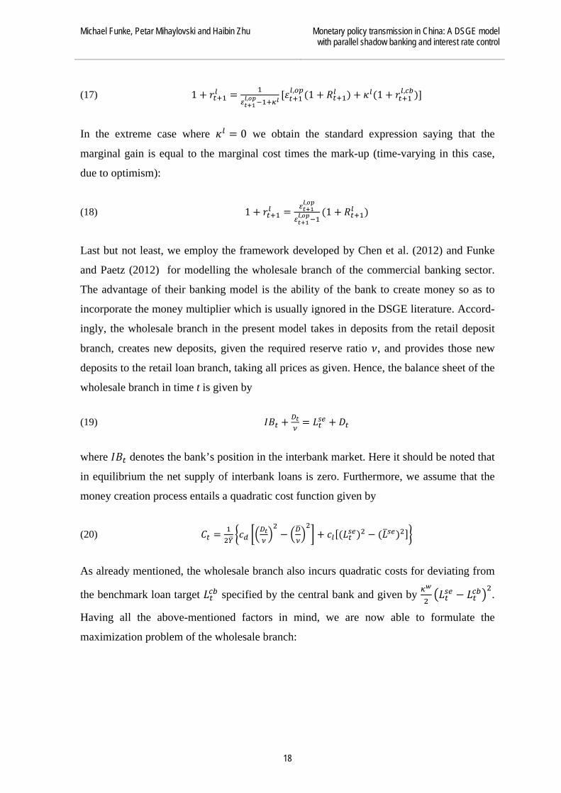
Last but not least, we employ the framework developed by Chen et al. (2012) and Funke
and Paetz (2012) for modelling the wholesale branch of the commercial banking sector.
The advantage of their banking model is the ability of the bank to create money so as to
incorporate the money multiplier which is usually ignored in the DSGE literature. Accord-
ingly, the wholesale branch in the present model takes in deposits from the retail deposit
branch, creates new deposits, given the required reserve ratio 𝜈, and provides those new
deposits to the retail loan branch, taking all prices as given. Hence, the balance sheet of the
wholesale branch in time t is given by
(19) 𝐼𝐵𝑡 + 𝐷𝑡
𝜈= 𝐿𝑡𝑠𝑒 + 𝐷𝑡
where 𝐼𝐵𝑡 denotes the bank’s position in the interbank market. Here it should be noted that
in equilibrium the net supply of interbank loans is zero. Furthermore, we assume that the
money creation process entails a quadratic cost function given by
(20) 𝐶𝑡 = 1
2𝑌��𝑐𝑑 ��
𝐷𝑡𝜈�2− �𝐷
�𝜈�2� + 𝑐𝑙[(𝐿𝑡𝑠𝑒)2 − (𝐿�𝑠𝑒)2]�
As already mentioned, the wholesale branch also incurs quadratic costs for deviating from
the benchmark loan target 𝐿𝑡𝑐𝑏 specified by the central bank and given by 𝜅𝑤
2�𝐿𝑡𝑠𝑒 − 𝐿𝑡𝑐𝑏�
2.
Having all the above-mentioned factors in mind, we are now able to formulate the
maximization problem of the wholesale branch:
18

BOFIT- Institute for Economies in Transition Bank of Finland
BOFIT Discussion Papers 9/ 2015
max
{𝐿𝑡𝑠𝑒,𝐷𝑡}
𝐸0 ∑ ∞𝑡=0 𝛽𝑤𝑏𝑡 {(1 + 𝑅𝑡𝑙)𝐿𝑡𝑠𝑒 − 𝐿𝑡+1𝑠𝑒 + (1 + 𝑅𝑡𝑅)𝐷𝑡 − 𝐷𝑡+1
(21)
−�(1+𝑅𝑡𝑑)𝐷𝑡𝜈
− 𝐷𝑡+1𝜈� − [(1 + 𝑅𝑡𝐼𝐵)𝐼𝐵𝑡 − 𝐼𝐵𝑡+1] − 𝜅𝑤
2�𝐿𝑡𝑠𝑒 − 𝐿𝑡𝑐𝑏�
2 − 𝐶𝑡}
Substituting the period budget constraint in equation (21) yields the following periodic
profit maximization problem.
(22) 𝐹𝑡𝑤𝑏 = (𝑅𝑡𝑙 − 𝑅𝑡𝐼𝐵)𝐿𝑡𝑠𝑒 + [(𝑅𝑡𝑅 − 𝑅𝑡𝐼𝐵) + 1
𝜈(𝑅𝑡𝐼𝐵 − 𝑅𝑡𝐷)]𝐷𝑡 −
𝜅𝑤
2�𝐿𝑡𝑠𝑒 − 𝐿𝑡𝑐𝑏�
2 − 𝐶𝑡
The optimal amount of deposits and loans is given by the first-order conditions and
illustrates the fact that the marginal benefit from each asset is equal to the opportunity cost
of holding it:
(23) 𝑅𝑡𝐷 = 𝑅𝑡𝐼𝐵 + 𝜈(𝑅𝑡𝑅 − 𝑅𝑡𝐼𝐵) − 𝑐𝑑
𝑌�𝐷𝑡𝜈
(24) 𝑅𝑡𝐿 = 𝑅𝑡𝐼𝐵 + 𝜅𝑤�𝐿𝑡𝑠𝑒 − 𝐿𝑡𝑐𝑏� + �𝑐𝑙
𝑌�� 𝐿𝑡𝑠𝑒
Equation (23) reveals that the opportunity cost of holding deposits is equal to the interbank
rate adjusted for the return on required reserves and the management cost entailed by the
production of new deposits. Similarly, Equation (24) illustrates that the opportunity cost
for loans is given by the interbank rate, the deviation from the window guidance loan
quota, and the management cost. Finally, closing the model entails a rule for the interbank
rate. In line with Gerali et al. (2010), we assume that the wholesale branch of the commer-
cial bank has unlimited access to the lending facility of the central bank. As a result, arbi-
trage ensures that 𝑅𝑡𝐼𝐵 = 𝑅𝑡.
3.2 Shadow banking and high-risk small and medium-sized firms This section introduces our approach to modelling shadow banking in the Chinese econ-
omy. The framework for modelling shadow banks’ behaviour in the present setup follows
Bernanke et al. (1999) and takes into account the Fisher-deflation effect emphasized by
Christensen and Dib (2008) and Iacoviello (2005), among many others. That is, we assume
the frictions arise on the firm level rather than on the side of the shadow bank. Nonethe-
19

Michael Funke, Petar Mihaylovski and Haibin Zhu Monetary policy transmission in China: A DSGE model with parallel shadow banking and interest rate control
less, bank´s net worth plays an important role in the current framework as the accumula-
tion of profits (losses) is possible due to biased expectations as to a high-risk firm’s pro-
ductivity level. This way of introducing bank equity in a DSGE model with perfectly com-
petitive financial sector has been proposed by Zhang (2009). The next paragraph sheds
light on the interaction between a perceived high potential high-risk firm and the shadow
banking sector.
High-risk firms, like their low-risk peers, own a share of the economy´s physical
stock of capital. They purchase it from capital producers and provide it to intermediate-
good firms for the production of intermediate goods. Moreover, since high-risk firms are
not able to self-finance their capital purchases and do not have access to the commercial
banking sector, they seek financing from the economy’s shadow banks. In the model, the
high-risk firms are fraught with risk because their own capital is subject to idiosyncratic
random productivity shocks in period t+1 equal to 𝜔𝑡+1. The latter is a random variable
assumed to be log-normally distributed:
(25) log (ω) ~ 𝑁 �− 1
2𝜎𝑠2,𝜎𝑠2�
Equation (25) implies 𝔼(𝜔) = 1. At the end of period t the high-risk firm decides on the
loan amount needed to purchase new capital, which is equal to the difference between the
expenditure on physical capital and the firm´s own net worth:
(26) 𝐿𝑡+1𝑟𝑒 = Q𝐾,�𝑡𝐾�𝑡+1𝑟𝑒 − 𝑁𝑡+1𝑟𝑒
At the end of period t the shadow bank offers a debt contract to the high-risk firm which
specifies the lending rate 𝑅𝑠𝑏 and the loan value 𝐿𝑟𝑒.9 In period t+1, the firm sees whether
the idiosyncratic shock to its capital stock is below or above a threshold level 𝜔�𝑡+1,
defined by
(27) 𝜔�𝑡+1(1 + 𝑅𝑡+1
𝑘,𝑟𝑒)Q𝐾,�𝑡𝐾�𝑡+1𝑟𝑒 = 𝑅𝑡+1𝑠𝑏 𝐿𝑡+1𝑟𝑒
If 𝜔𝑡+1 > 𝜔�𝑡+1 the firm remains solvent and pays the lender the principal as well as the
interest due on the loan, 𝑅𝑡+1𝑠𝑏 𝐿𝑡+1𝑟𝑒 . Accordingly the borrower is able to keep the value of
the remaining capital stock, given by (𝜔𝑡+1 − 𝜔�𝑡+1)(1 + 𝑅𝑡+1𝑘,𝑟𝑒)Q𝐾,�𝑡𝐾�𝑡+1𝑟𝑒 . On the other
9𝑅𝑠𝑏 is the only interest variable in the model and is to be interpreted as an overall return, i.e. 𝑅𝑠𝑏 = 1 + 𝑟𝑠𝑏.
20

BOFIT- Institute for Economies in Transition Bank of Finland
BOFIT Discussion Papers 9/ 2015
hand, if 𝜔𝑡+1 < 𝜔�𝑡+1, the firm declares bankruptcy and so receives nothing. Furthermore,
the insolvent firm undergoes monitoring by the bank, which appropriates what is left of the
capital stock after the occurrence of the shock. Hence, the shadow bank’s revenue in the
case of default of the firm is (1 − 𝜇)(1 + 𝑅𝑡+1𝑘,𝑟𝑒)𝜔𝑡+1Q𝐾,�𝑡𝐾�𝑡+1𝑟𝑒 . Unlike commercial finan-
cial intermediaries, shadow banks operate in perfectly competitive environment. The ad-
vantage of this assumption is that it renders the model simple enough and yet does not
leave out any of the important implications of the current paper. Then the zero-profit con-
dition of the bank is given by
(28) [1 − 𝐹𝑡(𝜔�𝑡+1)]𝑅𝑡+1𝑠𝑏 𝐿𝑡+1𝑟𝑒 + (1 − 𝜇)∫ 𝜔�𝑡+1
0 𝜔𝑑𝐹(𝜔)(1 + 𝑅𝑡+1𝑘,𝑟𝑒)Q𝐾,�𝑡𝐾�𝑡+1𝑟𝑒 = (1 + 𝑟𝑡+1𝐸 )𝐿𝑡+1𝑟𝑒
where 𝐹(𝜔) is the cumulative distribution function of 𝜔. Unlike Bernanke et al. (1999),
the opportunity cost of lending for the financial intermediary is not the risk-free rate.
Rather, shadow banks pay interest to their shareholders equal to 𝑟𝑡+1𝐸 . The latter will be
higher than the risk-free rate so long as the probability of default in the shadow banking
sector is positive. This framework is also employed by Zhang (2010) and Suh (2012). The
risky rate is equal to 𝑟𝑡+1𝐸 = (1+𝑟𝑡+1𝑑 )
(1−ϕ𝑡+1)− 1. Using the fact that 𝐺𝑡(𝜔�𝑡+1) = ∫ 𝜔�𝑡+1
0 𝜔𝑑𝐹(𝜔)
and Γ𝑡(𝜔�𝑡+1) = 𝜔�𝑡+1[1 − 𝐹𝑡(𝜔�𝑡+1)] + 𝐺𝑡(𝜔�𝑡+1), the shadow bank´s maximization
problem is given by
(29) max
{𝑘𝑡+1𝑟𝑒 ,𝜔�𝑡+1}
𝔼𝑡 �[1 − Γ𝑡(𝜔�𝑡+1)] 1+𝑅𝑡+1𝑘,𝑟𝑒
1+𝑟𝑡+1𝐸 𝑘𝑡+1𝑟𝑒 �
subject to
(30) [Γ𝑡(𝜔�𝑡+1) − 𝜇𝐺𝑡(𝜔�𝑡+1)] 1+𝑅𝑡+1
𝑘,𝑟𝑒
1+𝑟𝑡+1𝐸 𝑘𝑡+1𝑟𝑒 = 𝑘𝑡+1𝑟𝑒 − 1
where Γ𝑡(𝜔�𝑡+1) is the share of entrepreneurial profits received by the bank and 𝜇𝐺𝑡(𝜔�𝑡+1)
is the monitoring cost the bank expects to incur. Hence, 1 − Γ𝑡(𝜔�𝑡+1) is the share of the
profits received by the entrepreneur. Finally, 𝑘𝑡+1𝑟𝑒 =Q𝐾,�𝑡𝐾�𝑡+1
𝑟𝑒
𝑁𝑡+1𝑟𝑒 stands for the leverage ratio
of the risky firm. As in Bernanke et al. (1999) the solution to (30) leads to the expression
for the financial accelerator, given by
21
Michael Funke, Petar Mihaylovski and Haibin Zhu Monetary policy transmission in China: A DSGE model with parallel shadow banking and interest rate control
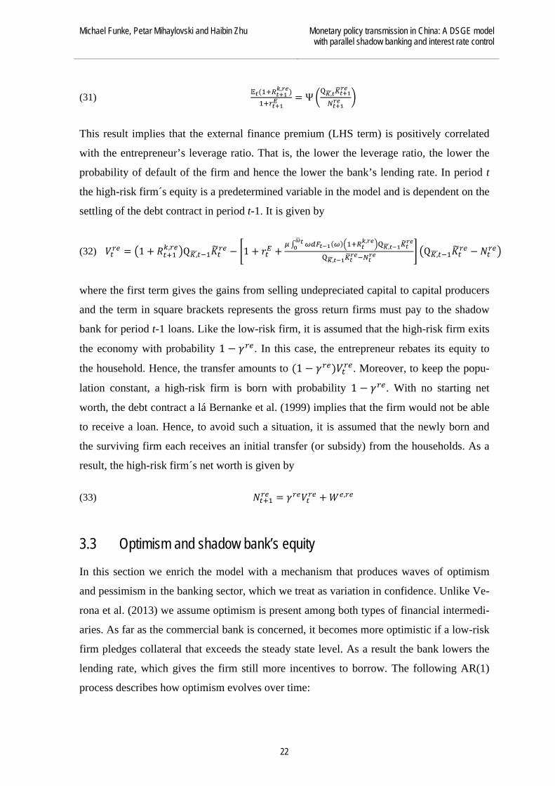
(31) 𝔼𝑡(1+𝑅𝑡+1
𝑘,𝑟𝑒)1+𝑟𝑡+1𝐸 = Ψ�
Q𝐾,�𝑡𝐾�𝑡+1𝑟𝑒
𝑁𝑡+1𝑟𝑒 �
This result implies that the external finance premium (LHS term) is positively correlated
with the entrepreneur’s leverage ratio. That is, the lower the leverage ratio, the lower the
probability of default of the firm and hence the lower the bank’s lending rate. In period t
the high-risk firm´s equity is a predetermined variable in the model and is dependent on the
settling of the debt contract in period t-1. It is given by
(32) 𝑉𝑡𝑟𝑒 = �1 + 𝑅𝑡+1𝑘,𝑟𝑒�Q𝐾,�𝑡−1𝐾�𝑡𝑟𝑒 − �1 + 𝑟𝑡𝐸 +
𝜇 ∫ 𝜔�𝑡0 𝜔𝑑𝐹𝑡−1(𝜔)�1+𝑅𝑡
𝑘,𝑟𝑒�Q𝐾,�𝑡−1𝐾�𝑡𝑟𝑒
Q𝐾,�𝑡−1𝐾�𝑡𝑟𝑒−𝑁𝑡
𝑟𝑒 � �Q𝐾,�𝑡−1𝐾�𝑡𝑟𝑒 − 𝑁𝑡𝑟𝑒�
where the first term gives the gains from selling undepreciated capital to capital producers
and the term in square brackets represents the gross return firms must pay to the shadow
bank for period t-1 loans. Like the low-risk firm, it is assumed that the high-risk firm exits
the economy with probability 1 − 𝛾𝑟𝑒. In this case, the entrepreneur rebates its equity to
the household. Hence, the transfer amounts to (1 − 𝛾𝑟𝑒)𝑉𝑡𝑟𝑒. Moreover, to keep the popu-
lation constant, a high-risk firm is born with probability 1 − 𝛾𝑟𝑒. With no starting net
worth, the debt contract a lá Bernanke et al. (1999) implies that the firm would not be able
to receive a loan. Hence, to avoid such a situation, it is assumed that the newly born and
the surviving firm each receives an initial transfer (or subsidy) from the households. As a
result, the high-risk firm´s net worth is given by
(33) 𝑁𝑡+1𝑟𝑒 = 𝛾𝑟𝑒𝑉𝑡𝑟𝑒 + 𝑊𝑒,𝑟𝑒
3.3 Optimism and shadow bank’s equity In this section we enrich the model with a mechanism that produces waves of optimism
and pessimism in the banking sector, which we treat as variation in confidence. Unlike Ve-
rona et al. (2013) we assume optimism is present among both types of financial intermedi-
aries. As far as the commercial bank is concerned, it becomes more optimistic if a low-risk
firm pledges collateral that exceeds the steady state level. As a result the bank lowers the
lending rate, which gives the firm still more incentives to borrow. The following AR(1)
process describes how optimism evolves over time:
22

BOFIT- Institute for Economies in Transition Bank of Finland
BOFIT Discussion Papers 9/ 2015
(34) 𝜒𝑡𝑟𝑏 = 𝜌𝜒𝑟𝑏𝜒𝑡−1𝑟𝑏 + (1 − 𝜌𝜒𝑟𝑏)𝛼𝑟𝑏(𝑁𝑡+1𝑠𝑒 − 𝑁�𝑠𝑒)
where 𝜒𝑡 is the level of optimism at time t, 𝜌𝑟𝑏 is the autoregressive parameter, 𝑁�𝑠𝑒 is the
steady-state value of the net worth of the low-risk firm and 𝛼𝑟𝑏 is the weight of the devia-
tion of the net worth in period t+1 from its steady state level. To be sure, our functional
form for the dynamics of optimism is assumed rather than derived from first principles.10
Equation (34) embeds the idea that the interest elasticity of credit demand depends upon
the level of optimism.
(35) 𝜀𝑡+1
𝑙,𝑜𝑝 = 𝜀𝑙(1 + 𝜒𝑡𝑟𝑏)
In a nutshell, equations (34) and (35) reveal that the higher the level of optimism, the
smaller the mark-up and the lower the lending rate charged by commercial banks. Before
discussing the law of motion for optimism in the shadow banking sector, we need first to
examine bank equity. In line with Zhang (2010) and Suh (2012), the shadow bank sets its
lending rate based on the expected return of the high-risk firm rather than on the realization
after the idiosyncratic shock has already been observed. As a result, in period t+1 the bank
might incur profits or losses. Furthermore, the shadow bank’s probability of default 𝜙𝑡 is
assumed to be log-normally distributed with mean equal to the intermediary's capital ratio
and standard deviation equal to 𝜎𝑠𝑏:
(36) 𝜅𝑡𝑠𝑏 = 𝑁𝑡
𝑠𝑏
𝐿𝑡𝑟𝑒
where 𝑁𝑡𝑠𝑏 is the shadow bank´s net worth and 𝐿𝑡𝑟𝑒 is the loan amount provided to the high-
risk firm. The model assumes that the shadow bank´s probability of default is represented
by
(37) 𝜙𝑡 = 𝑐𝑑𝑓(𝜅𝑡𝑠𝑏 ,𝜎𝑠𝑏)
where, as mentioned, 𝜅𝑡𝑠𝑏 and 𝜎𝑠𝑏 are the mean and standard deviation of 𝜙𝑡. Equation
(37) implies that the higher the capital ratio, the lower the probability of default and vice
10The modelling choice strikes a balance between the desire to enrich the dynamics of optimism and pessi-mism and the need for tractability of the model. We believe that the waves of optimism and pessimism reflect the time-varying uncertainty that confronts banks. We abstract from the deeper causes for the economic out-look for the sake of making progress in understanding its consequences.
23

Michael Funke, Petar Mihaylovski and Haibin Zhu Monetary policy transmission in China: A DSGE model with parallel shadow banking and interest rate control
versa. Consistent with the average of the capital-to-assets under management (AUM) ratio
over the 2010–2014 period, we set the capital ratio (below which the shadow bank is
deemed insolvent) at 3%. The shadow bank´s law of motion for net worth is given by
𝑁𝑡𝑠𝑏 = (1 − 𝜙𝑡−1)𝑁𝑡−1𝑠𝑏 + [1 − 𝐹𝑡(𝜔�𝑡𝑏)]𝑅𝑡𝑠𝑏𝐿𝑡𝑟𝑒 +
(38)
(1 − 𝜇)∫ 𝜔�𝑡𝑏
0 𝜔𝑑𝐹(𝜔)(1 + 𝑅𝑡𝑘,𝑟𝑒)Q𝐾,�𝑡−1𝐾�𝑡𝑟𝑒 − (1 + 𝑟𝑡𝐸)𝐿𝑡𝑟𝑒 + 𝑊𝑠𝑏
In words, current-period net worth is equal to previous period net worth excluding de-
faulted banks and including the profits from lending activity and the initial transfer from
households for the business start-up. By endogenizing the default probability of shadow
banks the model aims to capture the cyclical movement of risks in the economy. That is, if
trust companies’ net worth declines, the probability of default increases and thus investors
demand a higher premium over the risk-free rate. This is expected to have a negative im-
pact on lending, as firms’ funding costs rise. The possibility of profits in the shadow bank-
ing sector despite perfect competition results from the difference between the ex-ante
(𝜔�𝑡+1𝑎 ) and ex-post (𝜔�𝑡𝑏) default threshold levels. That is, equation (27) now becomes
(39) 𝜔�𝑎𝑡+1(1 + 𝔼𝑡𝑅𝑡+1
𝑘,𝑟𝑒)Q𝐾,�𝑡𝐾�𝑡+1𝑟𝑒 = 𝑅𝑡+1𝑠𝑏 𝐿𝑡+1𝑟𝑒
where 𝜔𝑡+1
𝑎 denotes the ex-ante default threshold level. In other words, the lending rate is
no longer state-contingent but is based on the expectation of the return to capital. Hence, in
period t+1 it is fixed and due to the idiosyncratic shocks to the high-risk firm’s capital pro-
ductivity, the shadow bank could incur profits or losses. The ex-post threshold value
(above which the risky firm remains solvent) is given by
(40) 𝜔�𝑏𝑡+1(1 + 𝑅𝑡+1
𝑘,𝑟𝑒)Q𝐾,�𝑡𝐾�𝑡+1𝑟𝑒 = 𝑅𝑡+1𝑠𝑏 𝐿𝑡+1𝑟𝑒
which leads to the following expression for 𝜔�𝑏𝑡+1:
(41) 𝜔�𝑡+1𝑏 = 𝜔�𝑡+1𝑎 (1+𝔼𝑡𝑅𝑡+1
𝑘,𝑟𝑒)(1+𝑅𝑡+1
𝑘,𝑟𝑒)
Equation (41) is the main engine by Zhang (2010) introduces the possibility of banks’ prof-
its. Nonetheless, neither Zhang (2010) nor Suh (2012) offers a possible explanation for the
24

BOFIT- Institute for Economies in Transition Bank of Finland
BOFIT Discussion Papers 9/ 2015
existence of the forecast error. The present setup aims at filling this gap and considers op-
timism in the shadow banking sector as a plausible cause of the discrepancy between the
forecasted and realized returns to capital. As is the case for the retail bank, in times of op-
timism (or pessimism) the trust company is prone to biased expectations regarding the pro-
ductivity of the high-risk firm’s physical. Consequently, equation (41) now becomes
(42) 𝜔�𝑡+1𝑏 = 𝜔�𝑡+1𝑎 (1+𝔼𝑡𝑅𝑡+1
𝑘,𝑟𝑒)(1+𝑅𝑡+1
𝑘,𝑟𝑒)= 𝜔�𝑡+1𝑎 (1 + 𝜒𝑡𝑠𝑏) ⇒ (1+𝔼𝑡𝑅𝑡+1
𝑘,𝑟𝑒)(1+𝑅𝑡+1
𝑘,𝑟𝑒)= (1 + 𝜒𝑡𝑠𝑏)
The law of motion for optimism in the shadow banking sector resembles that of the retail
bank
(43) 𝜒𝑡𝑠𝑏 = 𝜌𝜒𝑠𝑏𝜒𝑡−1𝑠𝑏 + (1 − 𝜌𝜒𝑠𝑏)𝛼𝑠𝑏(𝑁𝑡+1𝑟𝑒 − 𝑁�𝑟𝑒) ,
where all the variables are identical to those in equation (34) except that here they refer to
the level of optimism of the shadow bank and the net worth of the high-risk firm. As can
be seen, a higher level of optimism leads to a higher ex-post threshold default value for the
firm.
3.4 Monetary policy The descriptive evidence presented above indicates that PBoC currently uses a broader
range of instruments than its international peers in conducting monetary policy. To build a
unified theoretical framework for analysis, we incorporate the salient features of the non-
standard instruments and monetary policy transmission channels outlined above into our
DSGE framework.11 First, PBoC sets the short-term policy rate following a standard Tay-
lor-rule:
(44) 𝑅𝑡 = 𝜌�(𝑅𝑡−1) + (1 − 𝜌�)[𝑅� + 𝛼𝜋(𝜋𝑡 − 𝜋�) + 𝛼𝑦(𝑌𝑡 − 𝑌�)] + 𝜀𝑡𝑀𝑃
where 𝜋� is the steady-state inflation rate (assumed to be 1 in the DSGE literature), 𝑅� is the
steady-state short-term policy rate, and 𝑌� is the steady-state level of output. 𝛼𝜋 and 𝛼𝑦 are
the weights assigned to inflation and output, 𝜌� is the interest-rate smoothing parameter and
11The juxtaposition of various monetary policy instruments in Chen et al. (2012) and Funke and Paetz (2012) is a natural starting point for our subsequent analysis.
25

Michael Funke, Petar Mihaylovski and Haibin Zhu Monetary policy transmission in China: A DSGE model with parallel shadow banking and interest rate control
finally 𝜀𝑡𝑀𝑃 stands for the monetary policy shock. Furthermore, we assume that loan and
deposit rates in the commercial banking sector are restricted by the guidelines of the cen-
tral bank. Motivated by the pattern in Figure 1, we assume that the deposit rate ceiling in
the commercial banking sector is determined as follows:
(45) 𝑟𝑡𝑑 = min(𝑟𝑡
𝑑,𝑚𝑟 , 𝑟𝑡𝑑,𝑐𝑏)
where 𝑟𝑡
𝑑,𝑚𝑟 is the market-determined deposit rate, and 𝑟𝑡𝑑,𝑐𝑏 the deposit rate ceiling set by
the PBoC. Similarly, the lending rate in the commercial banking sector is determined by
(46) 𝑟𝑡𝑙 = max(𝑟𝑡
𝑙,𝑚𝑟 , 𝑟𝑡𝑙,𝑐𝑏)
where 𝑟𝑡
𝑙,𝑚𝑟 is the market-determined lending rate, and 𝑟𝑡𝑙,𝑐𝑏 is the respective lending rate
floor set by the PBoC. Since the two benchmark rates are rarely revised, we assume 𝑟𝑡𝑑,𝑐𝑏
and 𝑟𝑡𝑙,𝑐𝑏 to be exogenously given. In the baseline model calibrations below we assume that
the deposit rate ceiling in equation (45) is strictly binding. On the contrary, consistent with
Table 1 commercial banks are assumed to have some leeway in setting the lending rate.
Furthermore, PBoC steers the supply of credit in the commercial banking sector
via window guidance as part of its macroeconomic control policy.12 We assume that PBoC
determines the target for the total lending of commercial banks according to a Taylor-type
rule
(47) 𝐿𝑡𝑐𝑏 = ϕ𝑙𝑐𝑏�𝐿𝑡−1𝐶𝐵 � + �1 − ϕ𝑙𝑐𝑏��𝐿�𝑠𝑒 + ϕ𝑙𝑙[𝐿𝑡𝑠𝑒 − 𝐿�𝑠𝑒] + ϕ𝑙𝜋[𝜋𝑡 − 𝜋�] + ϕ𝑙
𝑦[𝑌𝑡 − 𝑌�]� + 𝜀𝑡𝑤𝑔
To interpret equation (47), recall that PBoC sets the loan quota in order to smooth inflation
and the output gap. In this connection, 𝜙𝑙𝜋 and 𝜙𝑙𝑦 represent the respective strengths of
monetary authority reactions to inflation and output growth and 𝜙𝜋𝑙 gives the persistence of
these responses. In addition, 𝜙𝑙𝑐𝑏 ensures that PBoC does not fully eliminate the loan sup-
ply during boom times when investment is on the rise. Furthermore, our model assumes
that the interest rate on required reserves passively mimics the PBoC’s policy rate, i.e.
𝑅𝑡𝑅 = 𝑅𝑡. Last but not least, 𝜀𝑡𝑤𝑔 is the window guidance shock. This terminates the de-
12Window guidance in China aimed at imposing lending targets is far from unique. For example, after the global recession 2008-2009 the UK government introduced lending targets for the five major UK banks to tackle the problem of reduced lending due to a weakening of bank balance sheets.
26

BOFIT- Institute for Economies in Transition Bank of Finland
BOFIT Discussion Papers 9/ 2015
scription of nonstandard monetary policy in China, which is absent from the expositions of
standard DSGE models.13
The rest of the model is standard and does not add sufficient intuition to warrant
inclusion in the main text. The interested reader is referred to Appendix A for a description
of the remaining model equations. In the remaining part of section 3, we define the interest
rate liberalization scenarios considered in the simulations.
3.5 Interest rate liberalization scenarios Chinese monetary policy is in a state of flux. In the baseline scenario, we model China’s
financial system such that the PBoC announces strictly binding benchmark deposit rates,
with a certain degree binding lending rates and “window guidance” on loan quotas, as
specified in section 3.4.14 The remaining two scenarios represent the stepwise financial
market liberalization. More precisely, we consider two different forms of interest rate lib-
eralization. In the first reform scenario, the central bank ends the control of interest rates
(i.e. the penalty function becomes zero) but window guidance on loan quotas remains. This
can be labelled as a “partial liberalization” scenario. In the second reform scenario, interest
rate control ends and window guidance is “turned off”.15 This will be termed the complete
liberalization scenario. The idea underlying the complete liberalization scenario is to cor-
rect the misallocation of credit in China. The way to do this is by raising the cost of funds
for banks. Raising deposit rates will narrow the banks’ net interest margin and put pressure
on them to raise lending rates. Higher lending rates will increase the likelihood that banks
find it profitable to lend to previously excluded firms and will force improved efficiency
on borrowers who have benefited from artificially low rates. The motivation for highlight-
ing the difference between these two reform scenarios is that removal of quota controls
13We do not consider a reaction function for the reserve requirements (v) because they are merely used to sterilize the domestic monetary consequences of foreign reserve inflows. 14In equation notation, the lending rate is given by 1 + 𝑟𝑡+1𝑙 = 1
𝜀𝑡+1𝑙,𝑜𝑝−1+𝜅𝑙
[𝜀𝑡+1𝑙,𝑜𝑝(1 + 𝑅𝑡+1𝑙 ) + 𝜅𝑙(1 + 𝑟𝑡+1
𝑙,𝑐𝑏)].
Hence, the parameter 𝜅𝑙 represents the penalty the bank incurs when the lending rate is below the benchmark rate set by the central bank. Since the lending rate is partially flexible, we set 𝜅𝑙=1 ∗ 𝜀𝑡+1
𝑙,𝑜𝑝. In other words, commercial banks set their rates approximately fifty-fifty determined by the market rate and the benchmark one. 15 To cite international experience, the objective of interest rate liberalization only involved removing interest rate control in most countries (e.g. in the US and Japan), but in some countries it also involved removing quantity control of credit (e.g. in Korea in early 1990s). See Liao and Tapsoba (2014) and Ito and Krueger (1996).
27

Michael Funke, Petar Mihaylovski and Haibin Zhu Monetary policy transmission in China: A DSGE model with parallel shadow banking and interest rate control
seems to be under-appreciated in the current discussion on China’s financial reform, as the
majority view is that the only step left in interest rate liberalization is to remove the upper
limit constraint on bank deposit rates.16
4 Calibrated parameters In calibrating the DSGE model presented above, we draw from a wide range of available
information. Parameters are selected in order to capture specific ratios in the Chinese
economy as closely as possible, with a view to the simulation properties of the model.
The discount factor 𝛽 is set to 0.9925 to match a steady-state deposit rate of 3%
on an annual basis whereas 𝜀𝑙,𝑜𝑝 and 𝜀𝑑 are assumed to equal 389 and –222, respectively.
This is done so as to match the average interest-rate spread (lending-deposit rate) of three
percentage points on an annual basis. The survival probability of the low-risk firm 𝛾𝑠𝑒 is
set at 0.96. The autoregressive parameter 𝜌𝜒𝑟𝑏 of the law of motion of optimism for the low-
risk firm is set at 0.95 since the process is highly persistent. Similarly, optimism in the
shadow banking sector is also assumed to be very persistent, albeit somewhat less than in
the commercial banking industry; hence, 𝜌𝜒𝑠𝑏 = 0.8. We assume that the share of firms fi-
nanced via the shadow (commercial) banking sector is 35% (65%). At end-2013, bank
lending amounted to about 126% of GDP and shadow banking (trust/WMP/AMP) to about
46% of GDP.17 Last but not least, in line with Zhang (2010) the model assumes the capital
adequacy ratio of the shadow bank is 10% in the steady state in order to match a steady-
state shadow bank default probability of 1%. The remaining parameters are set at standard
values in the DSGE literature and are summarized in Appendix B.
16A caveat to be stressed here is that although the direction is set, the path of further liberalization is highly uncertain. The Chinese government has not published an official roadmap and therefore the time-scales are still uncertain. 17Estimates of the size of the Chinese shadow banking sector vary widely depending on how it is defined. Li (2013: Table 1) has tied together various estimates for the years 2012/2013 ranging from 28% of GDP to 57% of GDP. For all the difficulties of making a reliable calculation, one thing is apparent: its very strong growth. A sensitivity analysis for alternative 𝜂 values is provided in Figure 11.
28

BOFIT- Institute for Economies in Transition Bank of Finland
BOFIT Discussion Papers 9/ 2015
5 Model properties Up to now the analysis has focused on the model description and calibration. Next we
delve more deeply into the quantitative model properties. At this point it is convenient to
explain our numerical solution method. We solve the nonlinear model with occasionally
binding constraints employing Guerrieri and Iacoviello´s (2014) linear first-order piece-
wise perturbation algorithm. The idea of the approach is to handle occasionally binding
constraints as different regimes of the same model. Under one regime, the occasionally
binding constraint is slack. Under the other regime, the same constraint is binding. As il-
lustrated below, the algorithm can handle the occasionally binding interest rate constraints
in China.
One way to learn about the model properties is to examine impulse response func-
tions (IRFs). The shocks that we consider are simple and abstract. Nevertheless, they are
intended to convey a rough idea of the DSGE model implications for observables. The first
two shocks considered are traditional demand and supply shocks. First we explore the re-
sponse of our key variables to a contractionary monetary policy shock. In this case, the de-
posit rate ceiling and window guidance create distortions in the baseline scenario. Then we
consider a supply shock. The supply shock is represented by a positive shock to an inter-
mediate-good firm´s productivity. Finally we trace out the effects of an expansionary win-
dow guidance shock. Below we examine each of these hypothetical experiments in turn.
5.1 Impact of a contractionary monetary policy shock In this section we consider an unexpected monetary tightening where the PBoC raises its
short-term policy rate by one percentage point. The solid black line gives the baseline sce-
nario results. The dashed red line and the dotted green line give the partial liberalization
scenario and the full liberalization scenario, respectively.18 The responses of selected ag-
gregate variables to a percentage point reduction of the short-term policy rate are shown in
Figure 5. Qualitatively almost all variables react as expected in all scenarios. The increase
in the policy rate leads to a decrease in investment. As a result output falls which drives
18Note that the horizontal axis in all IRF graphs measures quarters after the shock, and the horizontal axis are percent deviations from steady state values. For all interest rates, the absolute deviations from the steady state are given. For the remaining variables, percent deviations from the steady state are reported.
29

Michael Funke, Petar Mihaylovski and Haibin Zhu Monetary policy transmission in China: A DSGE model with parallel shadow banking and interest rate control
inflation down.19 In accordance with the notion of monetary neutrality, the temporal pattern
of output is hump-shaped back to its pre-shock level. In addition, higher deposit interest
rates in the shadow banking sector increase savings and reduce consumption. Furthermore,
the fall in asset prices induces a decrease in net worth of both types of firms, and negative
financial acceleration ensues. Noteworthy too is the horizontal segment of the deposit rate
IRF. This nicely illustrates how the occasionally binding constraint is imposed on the IRFs
by Guerrieri and Iacoviello’s (2014) linear first-order piecewise perturbation algorithm.
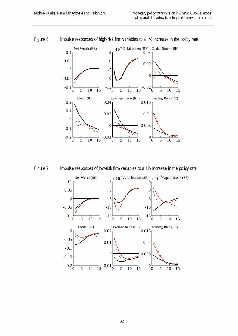
How responsive is lending to high-risk firms to changing money-market condi-
tions? In the first instance Figure 6 shows that shadow bank lending rates do react to
changes in monetary policy.20 Furthermore, Figure 6 and 7 illustrate that interest rate de-
regulation is an important factor in studying the behaviour of firm-specific variables. Fig-
ure 6 illustrates how high-risk firms react to a monetary contraction. It reveals the notable
feature that tighter regulation of interest rates in the commercial banking sector leads to an
increase in lending by the shadow banking sector. The interpretation of this result is
straightforward. Once the deposit rate ceiling becomes binding, an additional substitution
effect kicks in and “trusts” begin to engage in regulatory capital arbitrage via off-balance
sheet vehicles.21 In other words, “trusts” employ the loophole that interest rate and loan
restrictions do not apply to shadow banks. This allows them to offer higher deposit interest
rates which induces shadow banks to expand their balance sheet and leverage.22 As seen in
Figure 6, this establishes a commercial bank-like credit intermediation channel. Relatedly,
lending rates increase after a contractionary monetary policy shock across the board.
As shown in Figure 7, this induces low-risk firms to reduce the amount of capital
purchased and consequently also the demand for commercial bank loans. The flip side of
this is that commercial bank financing becomes more expensive relative to borrowing
money from the shadow banking sector. This gives rise to off-balance sheet shadow bank
lending and provides opportunities for the shadow banking sector to partially fill the gap.
19An implication is that the dynamics of the macroeconomic aggregates in response to shocks can be well approximated by a representative bank model. It fits into this picture that Fernald et al. (2014) have recently shown that monetary policy shocks generate standard IRF responses in a FAVAR framework, comprising an economic activity factor, an inflation factor, and the PBoC benchmark interest rate. 20This confirms the finding of Qin et al. (2014) that China´s informal lending rates are responsive to mone-tary policy. 21For empirical evidence on the regulatory arbitrage hypothesis, see Acharya et al. (2013). 22One needs to keep in mind that although shadow banks have been subject to restrictions on their leverage ratios and net capital requirements since 2010, the restrictions on their operations are still much looser than those for commercial banks. The fact that additional WMP sales allow the shadow banking sector to replace some of the lost commercial bank credit is consistent with the empirical evidence in Altunbas et al. (2009).
30

BOFIT- Institute for Economies in Transition Bank of Finland
BOFIT Discussion Papers 9/ 2015
In a nutshell, the reactions of lending by commercial banks and by shadow banks to a con-
tractionary monetary policy shock are in opposite directions. Whereas commercial banks
retrench, shadow banks proliferate and grow.23 This illustrates that an important measure to
discourage shadow banking is further interest rate liberalization. It has to be acknowl-
edged, however, that the additional off-balance sheet financial intermediation due to finan-
cial repression may increase the efficiency of the Chinese economy.24 Lastly, the evidence
for investment in Figure 5 indicates that window guidance has a restraining effect on the
fall in investment. Comparison of the dashed red line and the dotted green line reveals that
window guidance reduces capital decumulation by half.25
Figure 5 Impulse responses of selected aggregate variables to a 1% increase in the policy rate
23There is ample evidence that financial repression in developing countries encourages institutions to circum-vent it through nonbank intermediation. See, for example, Vittas (1992). 24Shadow banking can be conducive to further growth but also increase to risk. Allen et al. (2005), for exam-ple, have shown that shadow banking finance has bolstered SME growth in China. One of the conclusions to emerge is that the challenge for the Chinese regulators is to maximize the benefits of shadow banking while minimizing the systemic risks. It must be emphasized again that this paper does not address the regulatory issue of how to quantify empirically the real-world benefits and costs and thus enable one to maximize effi-ciency while minimizing risks. Luck and Schempp (2014) have shown that a large shadow banking sector may set the stage for a financial crisis. Plantin (2015) has studied the optimal degree of regulation when regu-latory arbitrage is present. 25One reason is that, in a model with forward-looking agents expectation effects exist, i.e. firms anticipate the window guidance reaction from the PBoC and factor it into their decision making.
0 5 10 15-10
-5
0
5x 10⁻³ Inflation
0 5 10 15-0.04
-0.03
-0.02
-0.01
0Investment
0 5 10 15-0.5
0
0.5
1Policy Rate
0 5 10 15-0.015
-0.01
-0.005
0Consumption
0 5 10 15-0.015
-0.01
-0.005
0Output
0 5 10 15-0.5
0
0.5
1
1.5Deposit Rate
31
Michael Funke, Petar Mihaylovski and Haibin Zhu Monetary policy transmission in China: A DSGE model with parallel shadow banking and interest rate control
Figure 6 Impulse responses of high-risk firm variables to a 1% increase in the policy rate
Figure 7 Impulse responses of low-risk firm variables to a 1% increase in the policy rate
0 5 10 15-0.1
-0.05
0
0.05
0.1Net Worth (RE)
0 5 10 15-15
-10
-5
0
5x 10⁻⁴C. Utilization (RE)
0 5 10 15-0.02
0
0.02
0.04Capital Stock (RE)
0 5 10 15-0.2
-0.1
0
0.1
0.2Loans (RE)
0 5 10 15-0.02
0
0.02
0.04Leverage Ratio (RE)
0 5 10 150
0.005
0.01
0.015Lending Rate (RE)
0 5 10 15-0.1
-0.05
0
0.05
0.1Net Worth (SE)
0 5 10 15-15
-10
-5
0
5x 10⁻⁴C. Utilization (SE)
0 5 10 15-15
-10
-5
0
5x 10⁻³ Capital Stock (SE)
0 5 10 15-0.2
-0.15
-0.1
-0.05
0Loans (SE)
0 5 10 15-0.01
0
0.01
0.02Leverage Ratio (SE)
0 5 10 150
0.005
0.01
0.015Lending Rate (SE)
32

BOFIT- Institute for Economies in Transition Bank of Finland
BOFIT Discussion Papers 9/ 2015
5.2 Impact of a positive technology shock to intermediate-good
firm’s productivity After looking at the effects of monetary policy shocks on both the real sector and financial
variables, it is worthwhile considering a supply-side shock. The reason for considering a
supply shock is that this creates a trade-off for PBoC, which aims at stabilizing inflation
and output. Furthermore, technology shocks are one of the main drivers of growth in an
emerging country like China. We assume that the technology shock to intermediate-good
firm´s productivity is highly persistent with an AR(1) coefficient of 0.9. Figure 8–10 give
the flavour of the monetary policy – interest rate liberalization interface.
Figure 8 Impulse responses of selected aggregate variables to a positive technology shock
0 10 20-2
-1
0
1x 10
-3 Inflation
0 10 20-10
-5
0
5x 10
-3 Investment
0 10 20-0.1
-0.05
0Policy Rate
0 10 200
2
4
6x 10
-3 Consumption
0 10 20-2
0
2
4x 10
-3 Output
0 10 20-0.2
-0.15
-0.1
-0.05
0Deposit Rate
33

Michael Funke, Petar Mihaylovski and Haibin Zhu Monetary policy transmission in China: A DSGE model with parallel shadow banking and interest rate control
Figure 9 Impulse responses of high-risk firm variables to a positive technology shock
Figure 10 Impulse responses of low-risk firm variables to a positive technology shock
Inspecting the results leads to the following conclusions. First, the aggregate variables in
Figure 8 closely resemble the typical IRF responses to a positive supply shock. As the
0 10 20-10
-5
0
5x 10
-3 Net Worth (RE)
0 10 20-10
-5
0
5x 10
-4 C. Utilization (RE)
0 10 20
-2
0
2
x 10-3 Capital Stock (RE)
0 10 20-0.04
-0.02
0
0.02
0.04Loans (RE)
0 10 20-5
0
5x 10
-3 Leverage Ratio (RE)
0 10 20-10
-5
0
5x 10
-4 Lending Rate (RE)
0 10 20-0.015
-0.01
-0.005
0Net Worth (SE)
0 10 20-1
-0.5
0x 10
-3 C. Utilization (SE)
0 10 20-4
-2
0
2x 10
-3Capital Stock (SE)
0 10 20
0
0.01
0.02
0.03Loans (SE)
0 10 200
2
4
6x 10
-3 Leverage Ratio (SE)
0 10 20-0.1
-0.05
0
0.05
0.1Lending Rate (SE)
34

BOFIT- Institute for Economies in Transition Bank of Finland
BOFIT Discussion Papers 9/ 2015
marginal productivity of capital rises, output exhibits positive steady state deviations from
trend while inflation recedes. Second, comparison of the case of full liberalization (dotted
green lines) vs. partial deregulation (dashed red lines) reveals that full liberalization results
in larger feed-through of the policy rate to the lending rate in Figure 9 and 10. From a
monetary policy point of view, the tighter the relationship between short-term and long-
term interest rates, the more effective is PBoC’s control along the yield curve. Thus, PBoC
has more scope to tailor monetary policy to macroeconomic conditions. Third, the full lib-
eralization scenario leads to a more pronounced rate shock transmission. The reason, as
before, is the effectiveness of window guidance. This subtle but important observation im-
plies that a given shock results in a larger feed-through to the loan level and investment.
The underlying reason is the financial intermediary channel of window guidance as a coun-
tervailing force. The difference between the partial reform scenario (dashed red lines) and
the full reform scenario (dotted green lines) reveals that leaning-against-the-wind window
guidance stabilizes the financing of firms by the commercial banking sector and thus coun-
teracts the technology shock.26 The next subsection completes the picture by shedding fur-
ther light on a window guidance shock.
5.3 Expansionary window guidance shock Next we investigate the effect of an expansionary window guidance shock, taking into ac-
count general equilibrium effects. In our framework, the window guidance shock is mod-
elled as an unexpected 10% expansion in the loan quotas in equation (47).27 Against the
background that window guidance still is a prominent quantity-based monetary instrument
of the PBoC, such an analysis is important for the effective design of future financial mar-
ket liberalization policies in China. Visually, the main results of the exercise are apparent
in Figure 11 and 12. The underlying assumption is the intermediate partial reform scenario
with window guidance. The experiment is conducted for two alternative shares of high-risk
firms in the economy and thus two different orders of magnitude of the shadow banking
sector. The dashed red line represents the results for η = 0.35, and the solid blue line for η
26This opens up the possibility of a vicious circle related to the co-existence of price-based monetary policy instruments and window guidance. The full effect of price-based instruments only comes into play when there is no window guidance influence involved. But as long as the interest rate instrument alone does not deliver the desired effects, the PBoC will rely on window guidance. 27We set the shock at 10% because this is the approximate magnitude of previous window guidance shocks [see Chen et al. (2012), Table 2, p. 6].
35
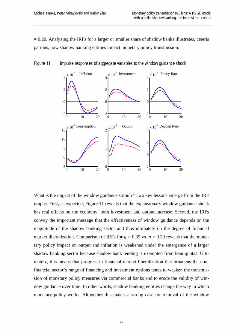
Michael Funke, Petar Mihaylovski and Haibin Zhu Monetary policy transmission in China: A DSGE model with parallel shadow banking and interest rate control
= 0.20. Analyzing the IRFs for a larger or smaller share of shadow banks illustrates, ceteris
paribus, how shadow banking entities impact monetary policy transmission.
Figure 11 Impulse responses of aggregate variables to the window guidance shock
What is the impact of the window guidance stimuli? Two key lessons emerge from the IRF
graphs. First, as expected, Figure 11 reveals that the expansionary window guidance shock
has real effects on the economy: both investment and output increase. Second, the IRFs
convey the important message that the effectiveness of window guidance depends on the
magnitude of the shadow banking sector and thus ultimately on the degree of financial
market liberalization. Comparison of IRFs for 𝜂 = 0.35 vs. 𝜂 = 0.20 reveals that the mone-
tary policy impact on output and inflation is weakened under the emergence of a larger
shadow banking sector because shadow bank lending is exempted from loan quotas. Ulti-
mately, this means that progress in financial market liberalization that broadens the non-
financial sector’s range of financing and investment options tends to weaken the transmis-
sion of monetary policy measures via commercial banks and to erode the validity of win-
dow guidance over time. In other words, shadow banking entities change the way in which
monetary policy works. Altogether this makes a strong case for removal of the window
0 10 20-2
0
2
4x 10
-4 Inflation
0 10 20-2
0
2
4x 10
-4 Investment
0 10 20-2
0
2
4x 10
-4 Policy Rate
0 10 20-5
0
5
10
15x 10
-5 Consumption
0 10 200
1
2x 10
-4 Output
0 10 20-2
0
2
4x 10
-4 Deposit Rate
36

BOFIT- Institute for Economies in Transition Bank of Finland
BOFIT Discussion Papers 9/ 2015
guidance toolbox under the complete liberalization scenario.28 In other words, the Chinese
authorities should end the heterodox policy mix of price-based and quantity-based mone-
tary policy instruments in the medium term. An even stronger case for the termination of
window guidance in the course of further financial market liberalization can be made if we
take into account the undermining of competition among commercial banks via prescribed
window guidance lending shares.
5.4 Shadow banking and welfare In the previous subsections we have described the functioning of monetary policy and the
dynamics of the shadow banking sector via impulse response functions. Now, we test the
effectiveness of both liberalization scenarios. The fundamental challenge for PBoC is how
to improve the allocation of loans without inducing economic and financial instability. To
evaluate the performance for the partial vs. the full reform scenario, we finally simulated
the model for 100,000 periods, ignoring the first 1,000. To compare both policy scenarios,
we simulated the model for each shock separately.29 Naturally, the evaluation depends on
the welfare function applied. The welfare criterion that we use to rank all scenarios, based
on a standard loss function, is to minimize the weighted sum of the variances of inflation
and output gap.
(48) Welfare Loss = Var(𝜋𝑡) + 𝛼𝑙Var(𝑌𝑡)
To be sure, equation (48) is assumed rather than derived from utility maximization.30 A
micro-founded version of the loss function derived from a second-order approximation of
the representative households’s utility function tends to give a low value of 𝛼𝑙. Since the
Chinese authorities care greatly about stabilizing output, a range of 1 < 𝛼𝑙 < 2 seems
appropriate.31
28This result bears some resemblance to that of Japan in the 1980s when financial liberalization and the asso-ciated expansion of various financial intermediary channels unrestrained by window guidance gradually un-dermined its effectiveness. 29The relevance of the way of proceeding results from the fact that countries have lived through a series of economic shocks, none of which were predicted by experts in real time. 30Note that the derivation from first principles is a futile endeavour due to the various agents and occasionally binding constraints. 31We let the weighting parameter 𝛼𝑙 vary within the range [1,2]. The qualitative results reported below re-main unaffected and are thus robust.
37

Michael Funke, Petar Mihaylovski and Haibin Zhu Monetary policy transmission in China: A DSGE model with parallel shadow banking and interest rate control
Table 2 Welfare loss of alternative policy scenarios for 𝜶𝒍 = 1.5
Policy scenario Contractionary monetary policy shock
Expansionary technology shock
Partial liberalization 2.9577e-04 1.8169e-05
Full liberalization 3.5006e-04 2.1096e-05
Full liberalization with a more aggressive Taylor Rule 2.6965e-04 1.8005e-05
Note: Taylor rule coefficients in the first three scenarios are 𝛼𝜋 = 1.8 and 𝛼𝑌 = 0.1, respectively. In the alternative more aggressive Taylor rule the coefficients are 𝛼𝜋 = 2.0 and 𝛼𝑌 = 0.2, respectively. Table 2 summarizes the results obtained for each shock and each scenario. In the first in-
stance, we compare the welfare effects for the two reform scenarios. What becomes obvi-
ous after the conduct of the analysis is that window guidance positively affects agents’
welfare. That is, the larger value of the loss function as between the two reform scenarios
is observed when the central bank abolishes both interest restrictions and loan quotas. This
reflects the counteracting window guidance effect of leaning against the wind, whereby the
PBoC opposes the accelerator and amplification mechanisms connected with the presence
of financial frictions. The other side of the coin is that when China liberalizes interest rates
further, greater volatility is a likely result.
The first two rows report the results of turning window guidance on or off in iso-
lation. Finally, we show the results for a more aggressive Taylor rule. In practice it is
highly unlikely that the parameters of the Taylor rule would remain constant after further
liberalization.32 Therefore, we revise the full liberalization scenario to incorporate induced
changes in the Taylor rule that compensate for the elimination of window guidance when
moving from the partial to the full liberalization scenario. For now, let us assume that 𝛼𝜋
and 𝛼𝑌 increase to 2.0 and 0.2, respectively. The simulations show that a more aggressive
Taylor rule with respect to inflation and the output gap leads to greater stability across the
board. All in all, the conclusion of this exercise is that full liberalization with a “hawkish”
PBoC produces an improvement in macroeconomic stabilization and is thus the preferred
policy option. Furthermore, the results indicate that waiving window guidance requires a
32Lucas (1976) has convincingly argued that the parameters of macroeconometric models are unlikely to re-main stable when policies change. This critique helped change the focus of policy evaluation from considera-tion of alternative paths of the policy instrument to consideration of rule shifts under alternative policy ap-proaches.
38

BOFIT- Institute for Economies in Transition Bank of Finland
BOFIT Discussion Papers 9/ 2015
new and active monetary policy approach that entails greater responsiveness in the short-
term monetary policy rate for loan targets.
6 Concluding remarks Ultimately, this paper is an attempt to provide some guidance on how to pursue financial
market liberalization in China. To this end, we have built a present-generation nonlinear
DSGE model with occasionally binding constraints that is tractable, versatile, and quantita-
tively potent. While not a crystal-ball, the DSGE model provides a well-organized concep-
tual framework for discussing the macroeconomic effects of financial market reforms in
China. The model is related to some recent papers on monetary policy alignment in DSGE
models with a banking sector and financial accelerator effects on both households and het-
erogeneous firms. Although the sequencing of financial market reforms and the optimal
institutional arrangement are clearly complex matters, both analytical reasoning and the
calibration results suggest some tentative policy conclusions. First, interest rate liberaliza-
tion will induce a more effective monetary policy transmission. Second, in China’s case,
interest rate liberalization not only involves removing interest rate control; it also involves
removing window guidance or quantity control on bank loans. In that sense, the prevailing
view that China is now only one step away (removing the upper bound limit of deposit
rates) from completing interest rate liberalization is not correct. Third, after interest rate
liberalization, economic activity could respond with more volatility to different shocks.
Fourth, liberalization of interest rates will attract deposits back into the commercial bank-
ing sector and rein in the expansion of the shadow banking sector. In short summary: The
results are of interest not merely for modelling purposes. Comparative evaluation of vari-
ous liberalization scenarios provides useful insights and could provide a more solid foun-
dation for future monetary policy in China.
Although the model captures several features of shadow banking in China and
leads to a novel set of economic insights, the modelling approach has some limitations and
therefore a few caveats are in order. First, on the conceptual side, what some of the litera-
ture does not always recognize, is that the numerical results are obtained in a linearized
unique-equilibrium model that rules out bubbles and other non-linear dynamics character-
izing crisis episodes. In other words, financial market instability is precluded by construc-
39

Michael Funke, Petar Mihaylovski and Haibin Zhu Monetary policy transmission in China: A DSGE model with parallel shadow banking and interest rate control
tion.33 Modelling such potential and highly nonlinear systemic risks and their evolution as
well as the regulatory responses of policymakers is beyond the DSGE´s conceptual reach.
Second, in the modelling framework all financial market variables reflect changes in fun-
damental values and are not associated with any type of irrational behaviour. Third, the
calibration exercise focuses on conceptual issues in the interpretation of the DSGE model
sketched above. In other words, the calibration exercise should be viewed as theory with
numbers, not empirical analysis in the strict sense of the term. Fourth, the IRFs consider
various shocks one at a time. Thus they defer the problem of identifying various shocks
and thus the sources of business cycle fluctuations in real time. Fifth, while DSGE models
provide rough orders of magnitude for shadow banking problems, recommendations for in-
depth financial reforms need to take into account complex political economy issues con-
straining reform implementation. All these issues are important avenues for future re-
search. In a nutshell, we consider the DSGE modelling exercise, with its virtues and limita-
tions, as a first step in a research agenda. An interesting cross-check of various results
would be to use Chinese microcensus data if such data were to become available. This
would enable the shedding of more light on the mechanisms underlying the link between
shadow banking and firm performance. In spite of these limitations, we believe the model-
ling setup explored here offers a useful tool for understanding monetary transmission as
well as the dynamics of the parallel shadow banking sector in China. It also offers some
useful policy implications and guidance for future financial market liberalization in China.
33 For a DSGE model with nonlinearities, see Benes et al. (2014). Olivier Blanchard has recently labelled the ignorance of the fact that small shocks could have large adverse effects the “dark corner” in macroeconom-ics. See http://www.imf.org/external/pubs/ft/fandd/2014/09/pdf/blanchard.pdf. Acemoglu et al. (2014) have recently characterized how the propagation and amplification of idiosyncratic microeconomic shocks can reshape the distribution of GDP and lead to deep recessions and sizable macroeconomic tail risks.
40

BOFIT- Institute for Economies in Transition Bank of Finland
BOFIT Discussion Papers 9/ 2015
References Acemoglu, D., Ozdaglar, A. and A. Tahbaz-Salehi (2014) “Microeconomic Origins of
Macroeconomic Tail Risks”, NBER Working Paper No. 20865, Cambridge (Mass.). Acharya, V.V., Schnabl, P. and G. Suarez (2013) “Securitization without Risk Transfer”,
Journal of Financial Economics 107, 515–536. Allen, F., Qian, J. and M. Qian (2005) “Law, Finance and Economic Growth in China”,
Journal of Financial Economics 77, 118–144. Altunbas, Y., Gambacorta, L. and D. Marquez-Ibanez (2009) “Securisation and the Bank
Lending Channel”, European Economic Review 53, 996–1009. Benes, J., Kumhof, M. and D. Laxton (2014) “Financial Crisis in DSGE Models: A
Prototype Model”, IMF Working Paper No. WP/14/57, Washington. Berlin, M. and L.J. Mester (1999) “Deposits and Relationship Lending”, Review of
Financial Studies 12, 579–607. Bernanke, B.S., Gertler, M. and S. Gilchrist (1999) “The Financial Accelerator in a
Quantitative Business Cycle Framework”, in: Taylor, J.B. and M. Woodford (eds.) Handbook of Macroeconomics, Vol. 1, 1341–1393, Amsterdam (Elsevier).
Calvo, G.A. (1983) “Staggered Prices in a Utility-Maximizing Framework”, Journal of Monetary Economics 12, 383–398.
Chen, Q., Funke, M. and M. Paetz (2012) “Market and Non-Market Monetary Policy Tools in a Calibrated DSGE Model for Mainland China”, BOFIT Discussion Paper No. 16/2012, Bank of Finland, Helsinki.
Christiano, L.J., Motto, R. and M. Rostagno (2010) “Financial Factors in Economic Fluctuations”, Working Paper No. 1192, European Central Bank, Frankfurt.
Fernald, J., Spiegel, M.M. and E.T. Swanson (2014) “Monetary Policy Effectiveness in China: Evidence from a FAVAR Model”, Journal of International Money and Finance 49, Part A, 83–103.
FSB (2013) Policy Framework for Strengthening Oversight and Regulation of Shadow Banking Entities, Basel (http://www.financialstabilityboard.org/wp-content/uploads/r_130829c.pdf?page_moved=1).
FSB (2014) Global Shadow Banking Monitoring Report 2014, Basel (http://www.financialstabilityboard.org/wp-content/uploads/r_141030.pdf).
Funke, M. and M. Paetz (2012) “Financial System Reforms and China's Monetary Policy Framework: A DSGE-Based Assessment of Initiatives and Proposals”, BOFIT Discussion Paper No. 30/2012, Bank of Finland, Helsinki.
Gerali, A., Neri, S., Sessa, F.M. and L. Signoretti (2010) “Credit and Banking in a DSGE Model of The Euro Area”; Journal of Money, Credit and Banking 42, 107–141.
Gertler, M. and P. Karadi (2010) “A Model of Unconventional Monetary Policy”, Journal of Monetary Economics 58, 17–34.
Guerrieri, L. and M. Iacoviello (2014) “OccBin: A Toolkit for Solving Dynamic Models With Occasionally Binding Constraints Easily”, Federal Reserve Board Working Paper No. 2014–47, Washington.
41

Michael Funke, Petar Mihaylovski and Haibin Zhu Monetary policy transmission in China: A DSGE model with parallel shadow banking and interest rate control
Iacoviello, M. (2005) “House Prices, Borrowing Constraints, and Monetary Policy in the
Business Cycle”, American Economic Review 95, 739–764. Iacoviello, M. (2014) “Financial Business Cycles”, Board of Governors of the Federal
Reserve System, International Finance Discussion Papers No. 1116, Washington. Ito, T. and A. Krueger (1996) Financial Deregulation and Integration in East Asia,
Chicago (University of Chicago Press). Li, C. (2013) “Shadow Banking in China: Expanding Scale, Evolving Structure”, Asia
Focus, April 2013, Federal Reserve Bank of San Francisco. Liao, W. and S. Tapsoba (2014) “China’s Monetary Policy and Interest Rate
Liberalization: Lessons from International Experiences”, IMF Working Paper No. WP/14/75, Washington.
Lucas, R.E. (1976) “Econometric Policy Evaluation: A Critique”, Carnegie-Rochester Conference Series on Public Policy 1, 19–46.
Luck, S. and P. Schempp (2014) “Banks, Shadow Banking, and Fragility”, ECB Working Paper No. 1726, Frankfurt.
Mazelis, F. (2014) “Monetary Policy Effects on Financial Intermediation via the Regulated and the Shadow Banking Systems”, Humboldt Universität zu Berlin, SFB 649 Discussion Paper Series No. 2014–056, Berlin.
Meeks, R., Nelson, B. and P. Alessandri (2014) “Shadow Banks and Macroeconomic Instability”, Bank of England Working Paper No. 487, London.
Plantin, G. (2015) “Shadow Banking and Bank Capital Regulation”, Review of Financial Studies 28, 146–175.
Qin, D., Zhong X. and X. Zhang (2014) “How Much Has Private Credit Lending Reacted to Monetary Policy in China? The Case of Wenzhou”, Journal of Asian Economics 31/32, 22–31.
Suh, H. (2012) “Evaluating Macroprudential Policy with Financial Friction DSGE Model”, Indiana University Bloomington, mimeo.
Verona, F., Martins, M.F. and I. Drumond (2013) “(Un)anticipated Monetary Policy in a DSGE Model with a Shadow Banking System”, International Journal of Central Banking 9, 73–117.
Vittas, D. (1992) Financial Regulation – Changing the Rules of the Game, Washington. Wu, J., Gyourko, J. and Y. Deng (2012) “Evaluating Conditions in Major Chinese Housing
Markets”, Regional Science & Urban Economics 42, 531–543. Zhang, J. (2014) Inside China's Shadow Banking: The Next Subprime Crisis?, New York
(Enrich Professional Publishing). Zhang, L. (2010) “Bank Capital Regulation, the Lending Channel and Business Cycles”,
Deutsche Bundesbank, Series 1, Economic Studies No. 33, Frankfurt. Zhang, L. and W. Xia, W. (2014) "Integrating Small and Medium-Sized Enterprises into
Global Trade Flows: The Case of China”, China Economic Review 23, 928–947.
42

BOFIT- Institute for Economies in Transition Bank of Finland
BOFIT Discussion Papers 9/ 2015
Appendix A Rest of the model
Households The infinitely-lived households in the model consume final goods, save and supply labour services monopolistically in order to maximize the expected value of their lifetime utility. The instantaneous utility function is given by
(A1) 𝑈𝑡 = 𝑙𝑜𝑔(𝐶𝑡 − 𝑏𝐶𝑡−1) − 𝜓𝑙ℎ𝑗,𝑡1+𝜎𝑙
1+𝜎𝑙 ,
where 𝐶𝑡 represents current consumption and ℎ𝑗,𝑡 is the representative household’s supply of working hours. The persistence of habit in the consumption pattern is captured by the parameter 𝑏 whereas 𝜓𝑙 is the preference parameter related to the disutility of labour. Fi-nally, 𝜎𝑙 stands for the disutility of labour and is the inverse of the Frisch elasticity of la-bour supply. The key difference regarding households in the current model vs. Verona et al. (2013) is in the saving behavior. In both modelling frameworks, the households are the only investors in the financial sector of the economy. Nonetheless, the Verona et al. (2013) model has a very simplified portfolio choice problem since households receive a certain (risk-free) return on their investment. Yet modelling the Chinese shadow banking sector entails the introduction of an asset which promises a higher but risky return. Accordingly they can either deposit their money in a savings account offered by the commercial bank-ing sector or purchase equity of the shadow bank.34 The former is risk-free since the Chi-nese government guarantees the returns on deposits whereas the latter is risky.35 The risk comes from the idiosyncratic return on capital that SMEs experience each period since part of their activity is financed by the shadow bank. Each period the household faces a budget constraint given by (1 + 𝑟𝑡𝐸)(1 − ϕ𝑡)𝐸𝑡−1 + (1 + 𝑟𝑡𝑑)𝐷𝑡−1 + 𝑊𝑗,𝑡ℎ𝑗,𝑡 + (1 − 𝛾𝑙)(1 − 𝜂)𝑉𝑡𝑠 + (A2) (1 − 𝛾𝑟)𝜂𝑉𝑡𝑟 + Π𝑡𝐼𝐺𝐹 + Π𝑟𝑏 + Π𝑠𝑏 − 𝐸𝑡 − 𝐷𝑡 − 𝑇𝑡 − 𝑃𝑡𝐶𝑡 ≥ 0
34One simplification, for the sake of tractability, is that we do not explore in depth potential determinants of the high household savings in China. Given China’s surplus of savings and a shortage of suitable vehicles for that thrift, it is easy to explain why investors are demanding WMP products. 35The argument ignores the fact that the de facto Chinese safety net for the banking sector is an ambivalent matter. On the one hand, the Chinese government announced on 30 November 2014 its plan to introduce a deposit insurance scheme which will not cover off-balance sheet vehicles. On the other hand, implicit Chi-nese state guarantees have recently been extended to shadow banks. When several off-balance sheet invest-ment products were on the verge of defaulting in 2014, the authorities orchestrated bail-outs. Therefore, it remains to be seen whether the de jure safety net is a time-consistent announcement, i.e. whether the gov-ernment will not stand any more behind uninsured deposits.
43

Michael Funke, Petar Mihaylovski and Haibin Zhu Monetary policy transmission in China: A DSGE model with parallel shadow banking and interest rate control
In words, in period t households receive the return on their equity investments from the previous period (1 + 𝑟𝑡𝐸)(1 − ϕ𝑡)𝐸𝑡−1. 𝜙𝑡 stands for the percentage of those shadow banking institutions which declared bankruptcy in period t-1 and essentially it represents the return shadow banks have to pay to investors. The equation makes it clear that in the non-bankruptcy state shadow banks have to promise a return higher than the risk-free rate on deposits because otherwise households would prefer to invest their money in the commercial banking sector. (1 + 𝑟𝑡𝑑)𝐷𝑡−1 is the safe return households receive each period as a liability on their deposits whereas 𝑊𝑗,𝑡ℎ𝑗,𝑡 represents their la-
bour income. The next two terms, (1 − 𝛾𝑙)(1 − 𝜂)𝑉𝑡𝑠 and (1 − 𝛾𝑟)𝜂𝑉𝑡𝑟, stand for the lump-sum transfers received from both high-risk and low-risk firms that exit the economy. Π𝑡𝐼𝐺𝐹, Π𝑟𝑏 and Π𝑠𝑏
are the last three terms in the income part of the budget constraint and represent respectively the profits of the intermediate-good firms and the commercial and the shadow banking sectors.36
The expenditure side of the household's budget constraint consists of investment in new shares (equity) 𝐸𝑡, the newly-made deposits 𝐷𝑡, lump-sum taxes paid by households 𝑇𝑡 and finally the nominal value of private consumption in period t, 𝑃𝑡𝐶𝑡. Hence, the max-imization problem of the representative household is given by
(A3) max{𝐶𝑡,𝐸𝑡,𝐷𝑡}
𝐸0 ∑ ∞𝑡=0 𝛽𝑡 �log(𝐶𝑡 − 𝑏𝐶𝑡−1) − 𝜓𝑙
ℎ𝑗,𝑡𝑟1+𝜎𝑙
1+𝜎𝑙�
subject to (1 + 𝑟𝑡𝐸)(1 − ϕ𝑡)𝐸𝑡−1 + (1 + 𝑟𝑡𝑑)𝐷𝑡−1 + 𝑊𝑗,𝑡ℎ𝑗,𝑡 + (1 − 𝛾𝑙)(1 − 𝜂)𝑉𝑡𝑠 + (A4) (1 − 𝛾𝑟)𝜂𝑉𝑡𝑟 + Π𝑡𝐼𝐺𝐹 + Π𝑟𝑏 + Π𝑠𝑏 − 𝐸𝑡 − 𝐷𝑡 − 𝑇𝑡 − 𝑃𝑡𝐶𝑡 ≥ 0 The solution of the maximization problem leads to the following first-order conditions with respect to 𝐶𝑡, 𝐸𝑡, and 𝐷𝑡: (A5) 𝑃𝑡𝜆𝑡 = 1
𝐶𝑡−𝑏𝐶𝑡−1− 𝛽𝑏 1
𝐶𝑡−𝑏𝐶𝑡−1
(A6) 𝜆𝑡 = 𝛽(1 + 𝑟𝑡+1𝐸 )(1 − ϕ𝑡+1)𝐸𝑡(𝜆𝑡+1) (A7) 𝜆𝑡 = 𝛽(1 + 𝑟𝑡+1𝑑 )𝐸𝑡(𝜆𝑡+1) where 𝜆𝑡 is the Lagrange multiplier (shadow price) associated with the budget constraint. As a result, we see that as long as the shadow bank’s default probability is positive, 𝑟𝐸 > 𝑟𝑑. This is the key difference between the present model and that of Verona et al. (2013), as the latter assumes that 𝑟𝐸 > 𝑟𝑑 in each period. The return on time deposits is a function of the central bank nominal interest rate and is risk-free. The labour supply deci-
36The shadow banking sector operates in a perfectly competitive environment. Nonetheless, profits are real-ized due to the difference between the ex-ante and ex-post default threshold levels for the high-risk firms.
44

BOFIT- Institute for Economies in Transition Bank of Finland
BOFIT Discussion Papers 9/ 2015
sion as well as the wage setting follows the baseline DSGE literature with both price and wage rigidities. In short, a labour agency bundles monopolistically provided and differenti-ated labour supply services of households and provides the aggregate to intermediate-good firms. Final-good firms The representative final-good firm competitively produces a final good 𝑌𝑡 using intermediate goods 𝑌𝑖,𝑡 using the Dixit-Stiglitz aggregator:
(A8) 𝑌𝑡 = [∫ 10 𝑌𝑖,𝑡
1𝜆𝑓𝑑𝑖]𝜆𝑓
where 𝜆𝑓 is the mark-up for the intermediate-good firms. The final-good firm maximizes its profits by choosing 𝑌𝑖,𝑡, taking as given the output price 𝑃𝑡 and the input prices 𝑃𝑖,𝑡 (A9) max
{𝑌𝑖,𝑡} 𝑃𝑡𝑌𝑡 − ∫ 10 𝑃𝑖,𝑡𝑌𝑖,𝑡𝑑𝑖
subject to
(A10) 𝑌𝑡 = [∫ 10 𝑌𝑖,𝑡
1𝜆𝑓𝑑𝑖]𝜆𝑓
The solution to the maximization problem leads to the following result:
(A11) 𝑌𝑖,𝑡 = �𝑃𝑖,𝑡𝑃𝑡�
𝜆𝑓1−𝜆𝑓 𝑌𝑡
where 𝑃𝑡 = [∫ 10 𝑃𝑖,𝑡
11−𝜆𝑓𝑑𝑖]1−𝜆𝑓.
Intermediate-good firms Intermediate-good firms operate in a monopolistic environment and produce differentiated intermediate goods according to the following Cobb-Douglas production function: (A12) 𝑌𝑖,𝑡 = exp(𝑎)𝐾𝑖,𝑡𝛼 𝐻𝑖,𝑡1−𝛼 where 𝑌𝑖,𝑡 is intermediate-good output, 𝛼 denotes the share of capital, 𝑎 is total factor pro-ductivity, and 𝐾𝑡 and 𝐻𝑡 are the capital and labour inputs.37 The intermediate-good firm
37 In line with the business cycle literature, we assume 𝑎 follows an AR(1) process with an autoregressive parameter 𝜌𝑎 = 0.9 and a positive innovation 𝜀~(0,𝜎𝑎2)
45

Michael Funke, Petar Mihaylovski and Haibin Zhu Monetary policy transmission in China: A DSGE model with parallel shadow banking and interest rate control
takes physical capital from both the high-risk and low-risk firms and bundles them into a single input. The CES aggregation formula is (A13) 𝐾𝑖,𝑡 = [η(𝐾𝑖,𝑡𝑟𝑒)𝜌 + (1 − 𝜂)(𝐾𝑖,𝑡𝑠𝑒)𝜌]
1𝜌
where 𝜌 stands for the degree of substitutability between both types of capital. When 𝜌 = 1, the capitals of the risky and safe entrepreneurs are perfectly substitutable. Each pe-riod the intermediate-good firm minimizes its cost function, solving the following minimi-zation problem: (A14) min
{𝐿𝑖,𝑡,𝐾𝑖,𝑡𝑟𝑒,𝐾𝑖,𝑡
𝑠𝑒}𝐶𝑡 = 𝑊𝑡𝐿𝑖,𝑡
𝑃𝑡+ 𝑟𝑡
𝑘,𝑟𝑒𝐾𝑖,𝑡𝑟𝑒 + 𝑟𝑡𝑘,𝑠𝑒𝐾𝑖,𝑡𝑠𝑒
subject to: (A15) 𝑌𝑖,𝑡 = 𝐾𝑖,𝑡𝛼 𝐻𝑖,𝑡1−𝛼 and (A16) 𝐾𝑖,𝑡 = [η(𝐾𝑖,𝑡𝑟𝑒)𝜌 + (1 − 𝜂)(𝐾𝑖,𝑡𝑠𝑒)𝜌]
1𝜌
As pointed out by Verona et al. (2013), since all firms face the same input prices and pro-duction technology, they also have the same marginal cost. As a result the "t" subscripts could be omitted. Firms’ marginal cost is thus given by
(A17) 𝑠𝑡 = [ 𝑤�𝑡1−𝛼
]1−𝛼
𝜌+𝛼(1−𝜌)[ 𝛼𝑟𝑡𝑘,𝑠𝑒 (𝐾𝑡𝑠𝑒)𝜌−1]−
𝛼𝜌+𝛼(1−𝜌)(𝑌𝑡)
𝛼(𝜌−1)𝜌+𝛼(1−𝜌) 𝜌
𝜌+𝛼(1−𝜌)
where 𝑤�𝑡 stands for the real wage in period t. The present model assumes intermediate-good firms set prices a lá Calvo (1983). That is, each period only 1 − 𝜉𝑝 of the firms are able to reoptimize their prices. The rest 𝜉𝑝 set their prices according to the following rule: (A18) 𝑃𝑖,𝑡 = 𝑃𝑖,𝑡−1(𝜋�)𝜄1(𝜋𝑡−1)1−𝜄1 where 𝜋 denotes the rate of inflation ( 𝜋� stands for steady-state inflation whereas 𝜋𝑡−1 =𝑃𝑡−1𝑃𝑡−2
) and 𝜄1 represents the degree of price indexation to steady-state inflation.38 Accord-
ingly the intermediate-good firm chooses the price level 𝑃𝑖 , 𝑡 = 𝑃�𝑖,𝑡 that maximizes its cur-rent and expected profits: (A19) max
{𝑃𝑖,𝑡}Π𝑡𝐼𝐹𝐺 = 𝐸0 ∑ ∞
𝑡=0 (𝛽𝜉𝑝)𝑡𝜆𝑡[(𝑃𝑖,𝑡 − 𝑆𝑡)𝑌𝑖,𝑡]
38 The derivation of staggered wages is identical to that of staggered prices. As a result we show only the latter. The interested reader may nevertheless refer to Appendix B of the earlier version of Verona et al. (2013) for all technical details related to wage stickiness.
46

BOFIT- Institute for Economies in Transition Bank of Finland
BOFIT Discussion Papers 9/ 2015
subject to (A20) 𝑌𝑖,𝑡 = �𝑃𝑖,𝑡
𝑃𝑡� 𝑌𝑡
where 𝑆𝑡 is the firm's nominal marginal cost and 𝛽 is the standard discount factor. In the solution to the standard sticky-price maximization problem above only a symmetric equi-librium is considered where, due to facing identical marginal costs, all firms set the same price 𝑃�𝑖,𝑡 = 𝑃�𝑡 and the aggregate price index is given by
(A21) 𝑃𝑡 = �(1 − 𝜉𝑝)𝑃�𝑡
11−𝜆𝑓 + 𝜉𝑝[𝑃𝑖,𝑡−1(𝜋�)𝜄1(𝜋𝑡−1)1−𝜄1]
11−𝜆𝑓�
1−𝜆𝑓
Capital producers Capital producers combine investment goods with undepreciated capital purchased from firms to produce new capital, which is then sold back to firms. At the end of period t the capital producers in the economy purchase the existing capital, 𝑥𝐾,𝑡, from firms and investment goods 𝐼𝑡 from the final-good firms. Then they combine these inputs in order to produce new capital 𝑥′𝐾,𝑡 according to the following law of motion: (A22) 𝑥′𝐾,𝑡 = 𝑥𝐾,𝑡 + 𝐴(𝐼𝑡 , 𝐼𝑡−1) It is assumed that there are no adjustment costs when transforming old capital into new whereas the transformation of investment goods into new capital is subject to quadratic costs represented by 𝐴(∙). Thus, the capital producer has the following maximization problem: (A23) max
{𝐼𝑡,𝑥𝐾,𝑡}𝔼0 ∑ ∞
𝑡=0 𝛽𝑡𝜆𝑡�Q𝐾,�𝑡[𝑥𝐾,𝑡 + 𝐴(𝐼𝑡 , 𝐼𝑡−1)] − Q𝐾,�𝑡𝑥𝐾,𝑡 − 𝑃𝑡𝐼𝑡�
The solution with respect to 𝑥𝐾,𝑡 leads to the conclusion that any value is profit maximiz-ing. Hence, (1 − 𝛿)𝐾�𝑡 satisfies this condition. The first-order condition with respect to 𝐼𝑡 yields the following expression (A24) 𝔼0[𝜆𝑡(Q𝐾,�𝑡𝐴1,𝑡 − 𝑃𝑡) + 𝛽𝜆𝑡+1Q𝐾,�𝑡+1𝐴2,𝑡] = 0 which is a standard Tobin's Q equation providing a link between the market price of capital and the marginal cost of producing investment goods and where 𝐴1,𝑡 = ∂𝐴(𝐼𝑡,𝐼𝑡−1)
∂𝐼𝑡 and
𝐴2,𝑡 = ∂𝐴(𝐼𝑡+1,𝐼𝑡)∂𝐼𝑡
. Finally, the law of motion for the evolution of the aggregate stock of
physical capital is given by (A25) 𝐾�𝑡+1 = 𝜂𝐾�𝑡+1𝑟𝑒 + (1 − 𝜂)𝐾�𝑡+1𝑠𝑒 = (1 − 𝛿)[𝜂𝐾�𝑡𝑟𝑒 + (1 − 𝜂)𝐾�𝑡𝑠𝑒] + 𝐴(𝐼𝑡 , 𝐼𝑡+1)
47

Michael Funke, Petar Mihaylovski and Haibin Zhu Monetary policy transmission in China: A DSGE model with parallel shadow banking and interest rate control
Aggregate variables and resource constraint The resource constraint in the economy is given by: (A26) 𝐶𝑡 + 𝐼𝑡 + 𝜂𝜇 ∫ 𝜔�𝑡
𝑏
0 𝜔𝑑𝐹(𝜔)(1 + 𝑅𝑡𝑘,𝑟𝑒)
Q𝐾,�𝑡−1𝐾�𝑡𝑟𝑒
𝑃𝑡+ 𝜂𝑎(𝑢𝑡𝑟𝑒)𝐾�𝑡𝑟𝑒 + (1 − 𝜂)𝑎(𝑢𝑡𝑠𝑒)𝐾�𝑡𝑠𝑒 = 𝑌𝑡
That is, aggregate demand consists of private consumption and investment. The last three terms represent respectively shadow banks' monitoring costs and firms' costs incurred in the capital utilization process. The aggregate net worth and aggregate leverage in the pre-sent set-up are given by the following equations: (A27) 𝑁𝑡+1
𝑎𝑔 = 𝜂𝑁𝑡+1𝑠𝑒 + (1 − 𝜂)𝑁𝑡+1𝑟𝑒 (A28) 𝑙𝑒𝑣𝑡+1
𝑎𝑔 = 𝜂𝑙𝑒𝑣𝑡+1𝑠𝑒 + (1 − 𝜂)𝑙𝑒𝑣𝑡+1𝑟𝑒 = 𝜂Q𝐾,�𝑡𝐾�𝑡+1
𝑟𝑒
𝑁𝑡+1𝑟𝑒 + (1 − 𝜂)
Q𝐾,�𝑡𝐾�𝑡+1𝑠𝑒
𝑁𝑡+1𝑠𝑒
The total amount of loans in the economy is equal to the weighted average of loans provided by both financial intermediaries: (A29) 𝐿𝑡+1
𝑎𝑔 = 𝜂𝐿𝑡+1𝑟𝑒 + (1 − 𝜂)𝐿𝑡+1𝑠𝑒 The market clearing conditions for renting capital from both firms are given by: (A30) ∫ 10 𝐾𝑖,𝑡𝑟𝑒𝑑𝑖 = 𝜂𝐾𝑡𝑟𝑒 = 𝜂𝑢𝑡𝑟𝑒𝐾�𝑡𝑟𝑒 and (A31) ∫ 10 𝐾𝑖,𝑡𝑠𝑒𝑑𝑖 = 𝜂𝐾𝑡𝑠𝑒 = 𝜂𝑢𝑡𝑠𝑒𝐾�𝑡𝑠𝑒 Finally, the total transfers from households to the firms and the shadow bank must satisfy: (A32) 𝑊𝑒 = 𝜂𝑊𝑡
𝑟𝑒,𝑒 + (1 − 𝜂)𝑊𝑡𝑠𝑒,𝑒
48

BOFIT- Institute for Economies in Transition Bank of Finland
BOFIT Discussion Papers 9/ 2015
Appendix B Model parameters
Agents Value Source Description
Households
𝛽 0.9925 Funke & Paetz (2012) Discount factor
𝜎𝑐 1 Funke & Paetz (2012) Risk-aversion coefficient
𝜎𝑙 1 Funke & Paetz (2012) Curvature of disutility of labour
𝜆𝑤 1.05 Christiano et al. (2010) Markup, workers
𝜄𝑤1 0.29 Christiano et al. (2010) Weight of wage indexation to steady-state inflation
𝜉𝑤 0.75 Our calibration Fraction of households that cannot reoptimize wage
b 0.8 Christiano et al. (2010) Habit persistence in consumption
Firms
𝛼 0.5 Funke & Paetz (2012) Capital share in the production function
𝜉𝑝 0.75 Erceg et al. (2000) Fraction of firms that cannot reoptimize
𝜄1 0.16 Christiano et al. (2010) Weight of price indexation to steady state inflation
𝜆𝑓 1.2 Christiano et al. (2010) Markup, intermediate good firms
S′′ 29.3 Christiano et al. (2010) Curvature of investment adjustment cost function
𝛿 0.03 Funke & Paetz (2012) Depreciation rate of capital
𝜌 0.78 Our calibration Degree of substitutability between capital services
Entrepreneurs
𝜎𝑎𝑟𝑒 18.9 Christiano et al. (2010) Curvature of capital utilization cost function (high-risk firm)
𝜎𝑎𝑠𝑒 18.9 Christiano et al. (2010) Curvature of capital utilization cost function (low-risk firm)
𝜇 0.3 Our calibration Fraction of realized profits lost in bankruptcy
𝜎𝑆 √0.68 Our calibration Steady state standard deviation of productivity shock
𝑊𝑒,𝑟𝑒 0.22 Christiano et al. (2010) Initial transfer from households to high-risk firms
𝑊𝑒,𝑠𝑒 0.14 Christiano et al. (2010) Initial transfer from households to low-risk firms
𝛾𝑟𝑒 0.95 Our calibration Survival probability of high-risk firms
𝛾𝑠𝑒 0.96 Our calibration Survival probability of low-risk firms
𝜂 0.35 Our calibration Share of high-risk firms
49

Michael Funke, Petar Mihaylovski and Haibin Zhu Monetary policy transmission in China: A DSGE model with parallel shadow banking and interest rate control
Agents Value Source Description
Banks
𝜌𝜒𝑟𝑏 0.9 Verona et al. (2013) Degree of persistence of optimism (commercial banks)
𝜌𝜒𝑐𝑏 0.8 Our calibration Degree of persistence of optimism (shadow banks)
𝛼𝑟𝑏 40 Verona et al. (2013) Sensitivity of optimism to low-risk firm’s net worth
𝛼𝑠𝑏 0.9 Our calibration Sensitivity of optimism to high-risk firm’s net worth
�̅�𝑟𝑏 0 Verona et al. (2013) Steady state level of optimism (commercial banks)
�̅�𝑠𝑏 0 Our calibration Steady state level of optimism (shadow banks)
𝜀𝑙 389 Our calibration Steady state level of lending rate elasticity
𝜀𝑑 –222 Our calibration Time-invariant deposit rate elasticity
𝜎𝑠𝑒 1.5504 Our calibration Standard deviation of shadow banks’ default rate
𝑐𝑑 0.01% Our calibration Cost parameter in the formal banking sector (deposit side)
𝑐𝑙 0.0158% Our calibration Cost parameter in the formal banking sector (lending side)
Policy and shock processes
ϕ𝑙𝑐𝑏 0.80 Our calibration Window guidance: sensitivity to policy rate variations
ϕ𝑙𝑙 0.30 Our calibration Window guidance: sensitivity to loans variations
ϕ𝑙𝜋 1.80 Our calibration Window guidance: sensitivity to inflation variations
ϕ𝑙𝑦 0.1 Our calibration Window guidance: sensitivity to output variations
𝜅𝑙 1 ∗ 𝜀𝑙 Our calibration Tightness of lending rate regulations
𝜅𝑤 0.40 Our calibration Window guidance sensitivity parameter
𝜈 0.2 Actual data Reserve ratio
𝜌� 0.9 Our calibration Policy rate autoregressive parameter
𝜌𝑎 0.9 Our calibration Autoregressive parameter of technology shock
𝛼𝜋 1.8 Our calibration Responsiveness of the Taylor rule to inflation
𝛼𝑦 0.1 Our calibration Responsiveness of Taylor rule to the output gap
50

BOFIT Discussion Papers A series devoted to academic studies by BOFIT economists and guest researchers. The focus is on works relevant for economic policy and economic developments in transition / emerging economies.
2013 No 21 Iftekhar Hasan, Krzysztof Jackowicz, Oskar Kowalewski and Łukasz Kozłowski: Market discipline during crisis:
Evidence from bank depositors in transition countries No 22 Yin-Wong Cheung and Risto Herrala: China’s capital controls – Through the prism of covered interest differentials No 23 Alexey Egorov and Olga Kovalenko: Structural features and interest-rate dynamics of Russia’s interbank lending market No 24 Boris Blagov and Michael Funke: The regime-dependent evolution of credibility: A fresh look at Hong Kong’s linked exchange rate system No 25 Jiandong Ju, Kang Shi and Shang-Jin Wei: Trade reforms and current account imbalances No 26 Marco Sanfilippo: Investing abroad from the bottom of the productivity ladder – BRICS multinationals in Europe No 27 Bruno Merlevede, Koen Schoors and Mariana Spatareanu: FDI spillovers and time since foreign entry No 28 Pierre Pessarossi and Laurent Weill: Do capital requirements affect bank efficiency? Evidence from China No 29 Irina Andrievskaya and Maria Semenova: Market discipline and the Russian interbank market No 30 Yasushi Nakamura: Soviet foreign trade and the money supply No 31 Anna Krupkina and Alexey Ponomarenko: Money demand models for Russia: A sectoral approach
2014 No 1 Vikas Kakkar and Isabel Yan: Determinants of real exchange rates: An empirical investigation No 2 Iftekhar Hasan, Krzysztof Jackowicz, Oskar Kowalewski and Łukasz Kozłowski: Politically connected firms in Poland and their access to bank financing No 3 Carsten A. Holz and Aaron Mehrotra: Wage and price dynamics in a large emerging economy: The case of China No 4 Zuzana Fungáčová, Anna Kochanova and Laurent Weill: Does money buy credit? Firm-level evidence on bribery and bank debt No 5 Jitka Poměnková, Jarko Fidrmuc and Iikka Korhonen: China and the World economy: Wavelet spectrum analysis of business cycles No 6 Christopher A. Hartwell: The impact of institutional volatility on financial volatility in transition economies: a GARCH family approach No 7 Christian Dreger, Tongsan Wang and Yanqun Zhang: Understanding Chinese consumption: The impact of hukou No 8 John Bonin, Iftekhar Hasan and Paul Wachtel: Banking in transition countries No 9 Chun-Yu Ho: Switching cost and deposit demand in China No 10 Zuzana Fungáčová and Laurent Weill: Understanding financial inclusion in China No 11 Anna Krupkina, Elena Deryugina and Alexey Ponomarenko: Estimating sustainable output growth in emerging market economies No 12 Qing He, Chang Xue and Chenqi Zhu: Financial Development and patterns of industrial specialization: Regional evidence from China No 13 Carsten A. Holz: Wage determination in China during the reform period No 14 Thorsten Beck, Hans Degryse, Ralph De Haas and Neeltje van Horen: When arm’s length is too far. Relationship banking over the business cycle No 15 Boris Blagov and Michael Funke: The credibility of Hong Kong’s currency board system: Looking through the prism of MS-VAR models with time-varying transition probabilities No 16 Philip Molyneux, Hong Liu and Chunxia Jiang: Bank capital, adjustment and ownership: Evidence from China No 17 Yin-Wong Cheung and Dagfinn Rime: The offshore renminbi exchange rate: Microstructure and links to the onshore market No 18 Marko Melolinna: What is the role of Emerging Asia in global oil prices? No 19 Yiwei Fang, Iftekhar Hasan and Lingxiang Li: Banking reform, risk-taking, and earnings quality – Evidence from transition countries No 20 Yanrui Wu: Local government debt and economic growth in China No 21 Christophe J. Godlewski, Rima Turk-Ariss and Laurent Weill: Do the type of sukuk and choice of shari’a scholar matter? No 22 Elena Deryugina and Alexey Ponomarenko: A large Bayesian vector autoregression model for Russia No 23 Yin-Wong Cheung, Menzie D. Chinn and Xingwang Qian: The structural behavior of China-US trade flows No 24 Claudio Cozza, Roberta Rabellotti and Marco Sanfilippo: The impact of outward FDI on the performance of Chinese multinationals
2015 No 1 Qing He, Liping Lu and Steven Ongena: Who gains from credit granted between firms? Evidence from inter-corporate loan announcements Made in China No 2 Ke Pang and Pierre L. Siklos: Macroeconomic consequences of the real-financial nexus: Imbalances and spillovers between China and the U.S. No 3 V.V. Mironov, A.V. Petronevich: Discovering the signs of Dutch disease in Russia No 4 Joshua Aizenman: The internationalization of the RMB, capital market openness, and financial reforms in China No 5 Yu-Fu Chen, Michael Funke and Kunyu Tao: Financial market reform – A new driver for China’s economic growth? No 6 Jarko Fidrmuc and Iikka Korhonen: Meta-analysis of Chinese business cycle correlation No 7 Jarko Fidrmuc, Zuzana Fungáčová and Laurent Weill: Does bank liquidity creation contribute to economic growth? Evidence from Russia No 8 Elena Deryugina, Olga Kovalenko, Irina Pantina and Alexey Ponomarenko: Disentangling loan demand and supply shocks in Russia No 9 Michael Funke, Petar Mihaylovski and Haibin Zhu: Monetary policy transmission in China: A DSGE model with parallel shadow banking and interest rate control
BOFIT Discussion Papers http://www.bof.fi/bofit_en • email: [email protected]
ISSN 1456-4564 (print) // ISSN 1456-5889 (online)