Monetary Law and Monetary Policy 4. Monetary policy – instruments and policies
Monetary Policy Report July 2017
Monetary Policy Report July 2017 ISSN 2313-9552 Online edition Publication date | July 2017 Central Bank of Argentina Reconquista 266 (C1003ABF) Ciudad Autónoma de Buenos Aires República Argentina Tel. | (54 11) 4000-1205 Web site | www.bcra.gob.ar Contents and edition | Economic Research Deputy General Management Publishing design | Communication Senior Management The contents of this report may be reproduced freely provided the source is acknowledged
For questions or comments please contact: [email protected]

Preface
As established in its Charter, the goal of the Central Bank of Argentina “is to promote monetary and financial
stability, employment, and economic development with social equity, to the extent of its powers and within
the framework of the policies implemented by the National Government”.
Without prejudice to the use of other, more specific instruments for complying with the rest of its mandates
—such as financial regulation and oversight, exchange market regulation, and innovation in savings, credit,
and means of payment instruments—, the main contribution that the monetary policy may offer to fulfill the
monetary authority’s mandates is to focus on price stability.
When inflation is low and stable, financial entities are able to better estimate their risks, which ensures higher
financial stability. Moreover, higher predictability allows producers and employers to create, endeavor,
produce and hire, which fosters investment and employment. Lastly, low income families may preserve the
value of their income and savings, which enables economic development with social equity.
The contribution of low and stable inflation to these objectives is never as evident as when it does not exist:
the flight from local currency may disrupt the financial system and lead to a crisis, the destruction of the price
system hinders productivity and genuine job creation, the inflation tax hits the most vulnerable families and
brings about redistribution of wealth that favor the most affluent segments of society. Low and stable
inflation, on the other hand, prevents all of these problems.
In line with this vision, the BCRA has formally adopted an Inflation Targeting Regime, effective as from
January 2017. As part of this new regime, the BCRA now releases its quarterly Monetary Policy Report. The
report’s main objectives are to communicate to the society the BCRA’s perspective of the recent inflationary
dynamic and its projection of price evolution, as well as to explain in a transparent manner its monetary
policy decisions.
Autonomous City of Buenos Aires, July 18th, 2017.
Contents
Page 5 | 1. Monetary Policy: Evaluation and Perspectives Page 8 | 2. International Context Page 16 | 3. Economic Activity Page 30 | Exhibit 1 / Private consumption, a difficult variable to monitor in real time Page 32 | Exhibit 2 / BCRA’s contemporary product forecast Page 35 | 4. Prices Page 41 | Exhibit 3 / National Consumer Price Index Page 44 | 5. Monetary Policy Page 53 | Exhibit 4 / An alternative look at the BCRA balance sheet Page 56 | Exhibit 5 / Movements in the high-powered money do not show changes in
monetary policy Page 59 | Abbreviations and Acronyms

Monetary Policy Report | July 2017
5
1. Monetary Policy: Assessment and Outlook The first complete semester have passed since the launch by the Central Bank of Argentina (BCRA) of the inflation targeting regime, in September, 2016. The targets are as follows: 12 % to 17 % for 2017, 10 % ± 2 percentage points (p.p.) for 2018, and 5 % ± 1,5 p.p. from 2019 onwards. At the beginning of the new regime, the BCRA established that the targets would be assessed based on the consumer price index with the greatest regional coverage among those published by the National Institute of Statistics and Census (INDEC). July, 11th marked the publication of the first National Consumer Price Index (CPI). According to that index, prices during the first half of the year increased by 11.8 %, a rate similar to that recorded in the Greater Buenos Aires Area (GBA), of 12 %. Inflation decreased systematically during the last year, as shown in the left-hand panel of Figure 1. So far this year, the national year-on-year inflation rate fell from 36.6 % (December, 2016) to 21.7 % (June, 2017). This last number is given by the combination of the CPI GBA figure up to December, 2016, and the national CPI figure from January, 2017 onwards. This inflation rate is the lowest since 2009.1
1 This comparison is based on the 7-province CPI prepared by CIFRA up to July, 2012; then the CPI of the city of Buenos Aires up to
April, 2016, then the CPI GBA up to May, 2017, and lastly the most recent nation-wide INDEC CPI figure.
Figure 1 | Consumer price indices
21.7
0
5
10
15
20
25
30
35
40
45
50
May‐16
Jun‐16
Jul‐16
Aug‐16
Sep‐16
Oct‐16
Nov‐16
Dec‐16
Jan‐17
Feb‐17
Mar‐17
Apr‐17
May‐17
Jun‐17
y.o.y. % chg.
CABA
Córdoba
San Luis
GBA
National*
Source: Statistical offices of City of Buenos Aires, San Luis, Córdoba and INDEC
1.3
0.0
0.5
1.0
1.5
2.0
2.5
3.0
3.5
4.0
May‐16
Jun‐16
Jul‐16
Aug‐16
Sep‐16
Oct‐16
Nov‐16
Dec‐16
Jan‐17
Feb‐17
Mar‐17
Apr‐17
May‐17
Jun‐17
Coremonthly % chg.
General level
CENTRAL BANK OF ARGENTINA
6
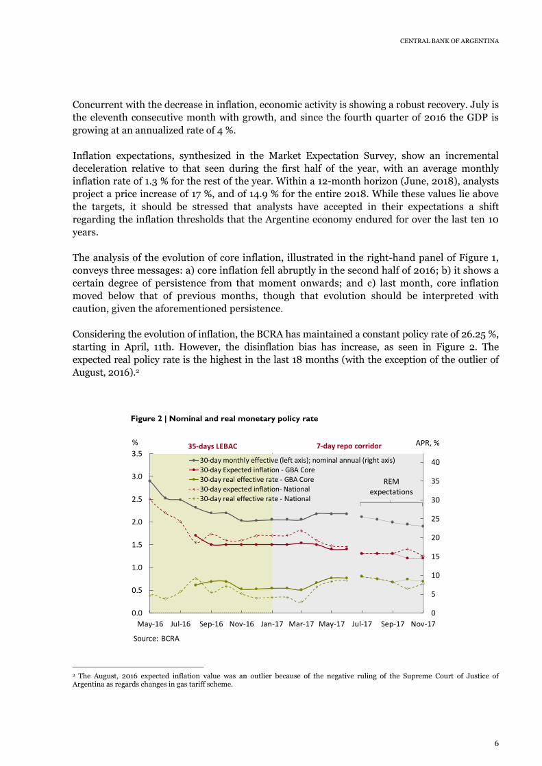
Concurrent with the decrease in inflation, economic activity is showing a robust recovery. July is the eleventh consecutive month with growth, and since the fourth quarter of 2016 the GDP is growing at an annualized rate of 4 %. Inflation expectations, synthesized in the Market Expectation Survey, show an incremental deceleration relative to that seen during the first half of the year, with an average monthly inflation rate of 1.3 % for the rest of the year. Within a 12-month horizon (June, 2018), analysts project a price increase of 17 %, and of 14.9 % for the entire 2018. While these values lie above the targets, it should be stressed that analysts have accepted in their expectations a shift regarding the inflation thresholds that the Argentine economy endured for over the last ten 10 years. The analysis of the evolution of core inflation, illustrated in the right-hand panel of Figure 1, conveys three messages: a) core inflation fell abruptly in the second half of 2016; b) it shows a certain degree of persistence from that moment onwards; and c) last month, core inflation moved below that of previous months, though that evolution should be interpreted with caution, given the aforementioned persistence. Considering the evolution of inflation, the BCRA has maintained a constant policy rate of 26.25 %, starting in April, 11th. However, the disinflation bias has increase, as seen in Figure 2. The expected real policy rate is the highest in the last 18 months (with the exception of the outlier of August, 2016).2
2 The August, 2016 expected inflation value was an outlier because of the negative ruling of the Supreme Court of Justice of Argentina as regards changes in gas tariff scheme.
Figure 2 | Nominal and real monetary policy rate
0
5
10
15
20
25
30
35
40
0.0
0.5
1.0
1.5
2.0
2.5
3.0
3.5
May‐16 Jul‐16 Sep‐16 Nov‐16 Jan‐17 Mar‐17 May‐17 Jul‐17 Sep‐17 Nov‐17
APR, %%
30‐day monthly effective (left axis); nominal annual (right axis)30‐day Expected inflation ‐ GBA Core30‐day real effective rate ‐ GBA Core30‐day expected inflation‐ National30‐day real effective rate ‐ National
REMexpectations
35‐days LEBAC 7‐day repo corridor
Source: BCRA

Monetary Policy Report | July 2017
7
The Central Bank will keep a clear disinflationary bias in order to ensure that the disinflation process moves towards the 12 % –17 % target and that inflation rate at end-2017 is consistent with the target of 10 % ± 2 p.p. for 2018.
CENTRAL BANK OF ARGENTINA
8
2. International Context
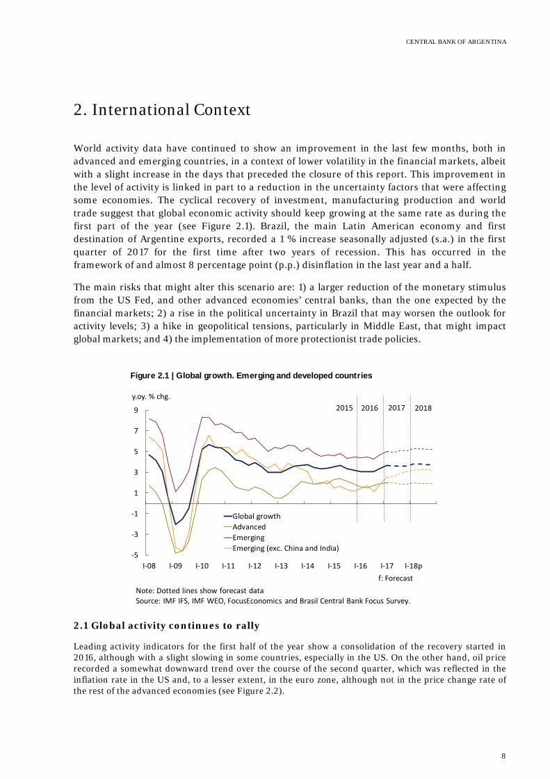
World activity data have continued to show an improvement in the last few months, both in advanced and emerging countries, in a context of lower volatility in the financial markets, albeit with a slight increase in the days that preceded the closure of this report. This improvement in the level of activity is linked in part to a reduction in the uncertainty factors that were affecting some economies. The cyclical recovery of investment, manufacturing production and world trade suggest that global economic activity should keep growing at the same rate as during the first part of the year (see Figure 2.1). Brazil, the main Latin American economy and first destination of Argentine exports, recorded a 1 % increase seasonally adjusted (s.a.) in the first quarter of 2017 for the first time after two years of recession. This has occurred in the framework of and almost 8 percentage point (p.p.) disinflation in the last year and a half.
The main risks that might alter this scenario are: 1) a larger reduction of the monetary stimulus from the US Fed, and other advanced economies’ central banks, than the one expected by the financial markets; 2) a rise in the political uncertainty in Brazil that may worsen the outlook for activity levels; 3) a hike in geopolitical tensions, particularly in Middle East, that might impact global markets; and 4) the implementation of more protectionist trade policies.
2.1 Global activity continues to rally
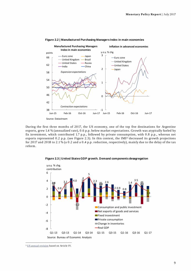
Leading activity indicators for the first half of the year show a consolidation of the recovery started in 2016, although with a slight slowing in some countries, especially in the US. On the other hand, oil price recorded a somewhat downward trend over the course of the second quarter, which was reflected in the inflation rate in the US and, to a lesser extent, in the euro zone, although not in the price change rate of the rest of the advanced economies (see Figure 2.2).
Figure 2.1 | Global growth. Emerging and developed countries
‐5
‐3
‐1
1
3
5
7
9
I‐08 I‐09 I‐10 I‐11 I‐12 I‐13 I‐14 I‐15 I‐16 I‐17 I‐18p
y.oy. % chg.
f: Forecast
Global growth
Advanced
Emerging
Emerging (exc. China and India)
Note: Dotted lines show forecast dataSource: IMF IFS, IMF WEO, FocusEconomics and Brasil Central Bank Focus Survey.
2016 20172015 2018
Monetary Policy Report | July 2017
9
During the first three months of 2017, the US economy, one of the top five destinations for Argentine exports, grew 1.4 % (annualized rate), 0.6 p.p. below market expectations. Growth was atypically fueled by fix investment, which contributed 1.7 p.p., followed by private consumption, with 0.8 p.p., whereas net exports represented 0.2 p.p. (see Figure 2.3). In this context, the IMF3 decreased its growth projections for 2017 and 2018 to 2.1 % (a 0.2 and a 0.4 p.p. reduction, respectively), mainly due to the delay of the tax reform.
3 US annual revision based on Article IV.
Figure 2.2 | Manufactured Purchasing Managers Index in main economies
Figure 2.3 | United States GDP growth. Demand components desagregation
38
42
46
50
54
58
62
66
Jun‐15 Feb‐16 Oct‐16 Jun‐17
Euro zone Japan
United Kingdom Brazil
United States Russia
India China
Source: Datastream
Contraction expectations
Expansion expectations
points
Manufactured Purchasing Managers Index in main economies
‐1
0
1
2
3
Jun‐15 Feb‐16 Oct‐16 Jun‐17
Euro zone
United Kingdom
United States
Japan
y.o.y. % chg.
Inflation in advanced economies
2.8
0.8
3.1 4.0
‐1.2
4
5
2.32.0
2.6
2 0.9 0.8
1.43.5
2.1
1.4
‐8
‐6
‐4
‐2
0
2
4
6
Q1‐13 Q3‐13 Q1‐14 Q3‐14 Q1‐15 Q3‐15 Q1‐16 Q3‐16 Q1‐17
y.o.y. % chg. contribution
Consumption and public investment
Net exports of goods and services
Fixed insvestment
Private consumption
Change in inventories
Real GDP
Source: Bureau of Economic Analysis
CENTRAL BANK OF ARGENTINA
10
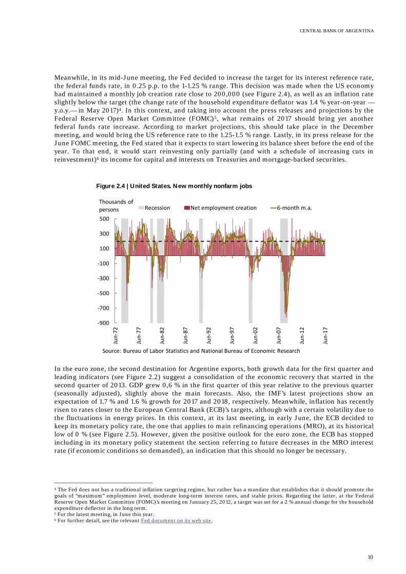
Meanwhile, in its mid-June meeting, the Fed decided to increase the target for its interest reference rate, the federal funds rate, in 0.25 p.p. to the 1-1.25 % range. This decision was made when the US economy had maintained a monthly job creation rate close to 200,000 (see Figure 2.4), as well as an inflation rate slightly below the target (the change rate of the household expenditure deflator was 1.4 % year-on-year —y.o.y.— in May 2017)4. In this context, and taking into account the press releases and projections by the Federal Reserve Open Market Committee (FOMC)5, what remains of 2017 should bring yet another federal funds rate increase. According to market projections, this should take place in the December meeting, and would bring the US reference rate to the 1.25-1.5 % range. Lastly, in its press release for the June FOMC meeting, the Fed stated that it expects to start lowering its balance sheet before the end of the year. To that end, it would start reinvesting only partially (and with a schedule of increasing cuts in reinvestment)6 its income for capital and interests on Treasuries and mortgage-backed securities.
In the euro zone, the second destination for Argentine exports, both growth data for the first quarter and leading indicators (see Figure 2.2) suggest a consolidation of the economic recovery that started in the second quarter of 2013. GDP grew 0,6 % in the first quarter of this year relative to the previous quarter (seasonally adjusted), slightly above the main forecasts. Also, the IMF’s latest projections show an expectation of 1.7 % and 1.6 % growth for 2017 and 2018, respectively. Meanwhile, inflation has recently risen to rates closer to the European Central Bank (ECB)’s targets, although with a certain volatility due to the fluctuations in energy prices. In this context, at its last meeting, in early June, the ECB decided to keep its monetary policy rate, the one that applies to main refinancing operations (MRO), at its historical low of 0 % (see Figure 2.5). However, given the positive outlook for the euro zone, the ECB has stopped including in its monetary policy statement the section referring to future decreases in the MRO interest rate (if economic conditions so demanded), an indication that this should no longer be necessary.
4 The Fed does not has a traditional inflation targeting regime, but rather has a mandate that establishes that it should promote the goals of “maximum” employment level, moderate long-term interest rates, and stable prices. Regarding the latter, at the Federal Reserve Open Market Committee (FOMC)’s meeting on January 25, 2012, a target was set for a 2 % annual change for the household expenditure deflector in the long term. 5 For the latest meeting, in June this year. 6 For further detail, see the relevant Fed document on its web site.
Figure 2.4 | United States. New monthly nonfarm jobs
‐900
‐700
‐500
‐300
‐100
100
300
500
Jun‐72
Jun‐77
Jun‐82
Jun‐87
Jun‐92
Jun‐97
Jun‐02
Jun‐07
Jun‐12
Jun‐17
Recession Net employment creation 6‐month m.a.Thousands of persons
Source: Bureau of Labor Statistics and National Bureau of Economic Research

Monetary Policy Report | July 2017
11
The outlook for the Chinese economy, the third destination for Argentine exports, has continued to improve, although there remain certain risks associated with the high indebtedness and real estate price levels, given their disruptive potential for the financial system. The Chinese authorities have accelerated the adoption of measures to deal with those risks.
As for activity indicators, the Asian giant reached its growth target for 2016 (a 6.5 to 7 % GDP increase), and, based on available information and on IMF estimations, the target should be reached this year as well. Activity data for the second quarter of 2017 show an expansion of economic activity equal to that
Figure 2.5 | Euro zone. Inflation and monetary indicators
Figure 2.6 | China. GDP growth
‐1
0
1
2
3
4
5
6
Jan‐06 Jul‐07 Jan‐09 Jul‐10 Jan‐12 Jul‐13 Jan‐15 Jul‐16
%
monetary policy rate
Inflation rate
Inflation target
Rate corridor
Source: ECB and Eurostat
4
5
6
7
8
9
10
11
12
13
Q1‐10 Q1‐11 Q1‐12 Q1‐13 Q1‐14 Q1‐15 Q1‐16 Q1‐17 Q1‐18f
y.o.y. % chg.
f: ForecastSource: FocusEconomics

CENTRAL BANK OF ARGENTINA
12
experienced in the first quarter of the year, 6.9 % y.o.y. (see Figure 2.6), whereas the June IMF projections (above those released in April)7 estimate a 6.7 % GDP growth this year and 6.4 % the next.
In Brazil —the main economy in the Latin American region and first destination for Argentine exports—, in the first quarter of 2017, and after eight consecutive quarters of reductions in the level of activity, GDP recorded a 1 % increase relative to the previous quarter (seasonally adjusted). At the same time, other activity indicators, such as the economic activity index —calculated by the Central Bank of Brazil (CBB)— and the industrial production index, have started showing positive change rates. Nevertheless, unemployment levels almost double those of 2014. In a context in which political uncertainty remains high, the latest projections from the Focus market expectations survey —carried out by the CBB— show that activity is expected to rise 0.3 % this year and 2.0 % the next.
Inflation projections from the Focus survey suggest that a CPI change rate of around 3.3 % is expected for 2017, and 4.2 % for 2018, both figures being within the inflation target (4.5 % ± 1.5 p.p.)8. The latest available inflation data shows a 3 % increase in the CPI in June, an indication of a disinflation process of almost 8 p.p. in 18 months (see Figure 2.7 and the Box in Section 5. Monetary Policy). Therefore, the CBB is expected to continue lowering its monetary policy rate, the target for the Selic rate, which has been on a downward trend since October 2016, having lost 4 p.p. to 10.25 %. Respondents of the Focus survey also forecast that the CBB will cut that target in 2.25 p.p. for the rest of 2017, which would leave the rate at 8 % at year-end.
2.2 Improving and less volatile international financial markets
International financial markets have continued to improve and lower volatility after the uncertainty created by the US election. So much so that most stock market indicators have maintained their upward path, particularly the Nikkei index in Japan and the stock market indexes in emerging markets, while yields of sovereign debt securities have remained relatively constant (with a slight downward trend).
7 April and June projections pertaining to the April 2017 World Economic Outlook and the annual review for China according to Article IV, respectively. 8 Brazil’s National Monetary Council has recently reduced the inflation target for 2019 to 4.25 % ± 1.5 p.p., and to 4 % ± 1.5 p.p. for 2020.
Figure 2.7 | Brazil. Macroeconomic indicators
‐8
‐6
‐4
‐2
0
2
4
6
8
10
12
14
0
2
4
6
8
10
12
14
16
18
20
22
Jan‐04 Jan‐06 Jan‐08 Jan‐10 Jan‐12 Jan‐14 Jan‐16
y.o.y. % chg.%
Source: Central Bank of Brazil
Policy interest rate
Policy real interest rate
Inlfation rate
Economic activity index (y.o.y. % chg.)
Monetary Policy Report | July 2017
13
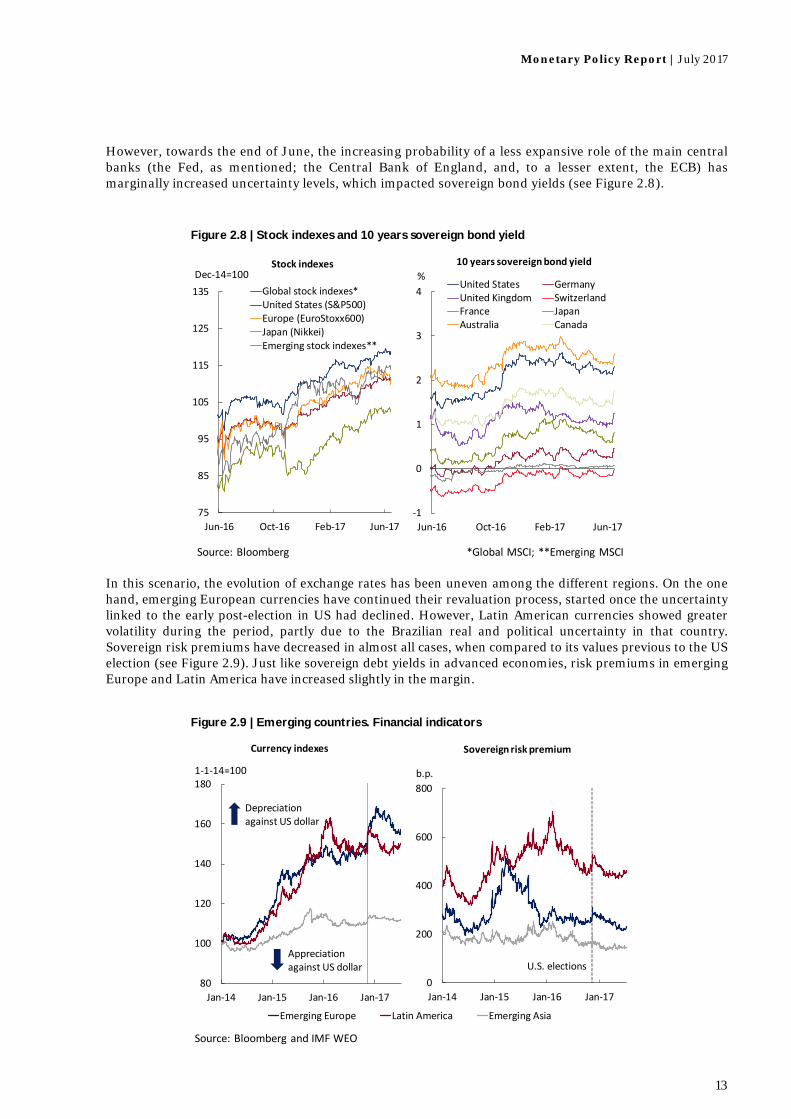
However, towards the end of June, the increasing probability of a less expansive role of the main central banks (the Fed, as mentioned; the Central Bank of England, and, to a lesser extent, the ECB) has marginally increased uncertainty levels, which impacted sovereign bond yields (see Figure 2.8).
In this scenario, the evolution of exchange rates has been uneven among the different regions. On the one hand, emerging European currencies have continued their revaluation process, started once the uncertainty linked to the early post-election in US had declined. However, Latin American currencies showed greater volatility during the period, partly due to the Brazilian real and political uncertainty in that country. Sovereign risk premiums have decreased in almost all cases, when compared to its values previous to the US election (see Figure 2.9). Just like sovereign debt yields in advanced economies, risk premiums in emerging Europe and Latin America have increased slightly in the margin.
Figure 2.8 | Stock indexes and 10 years sovereign bond yield
Figure 2.9 | Emerging countries. Financial indicators
‐1
0
1
2
3
4
Jun‐16 Oct‐16 Feb‐17 Jun‐17
United States GermanyUnited Kingdom SwitzerlandFrance JapanAustralia Canada
%
Source: Bloomberg *Global MSCI; **Emerging MSCI
75
85
95
105
115
125
135
Jun‐16 Oct‐16 Feb‐17 Jun‐17
Global stock indexes*United States (S&P500)Europe (EuroStoxx600)Japan (Nikkei)Emerging stock indexes**
Dec‐14=100Stock indexes 10 years sovereign bond yield
Source: Bloomberg and IMF WEO
80
100
120
140
160
180
Jan‐14 Jan‐15 Jan‐16 Jan‐17
Currency indexes
Emerging Europe Latin America Emerging Asia
Depreciation against US dollar
Appreciation against US dollar
1‐1‐14=100
0
200
400
600
800
Jan‐14 Jan‐15 Jan‐16 Jan‐17
Sovereign risk premium
U.S. elections
b.p.
CENTRAL BANK OF ARGENTINA
14
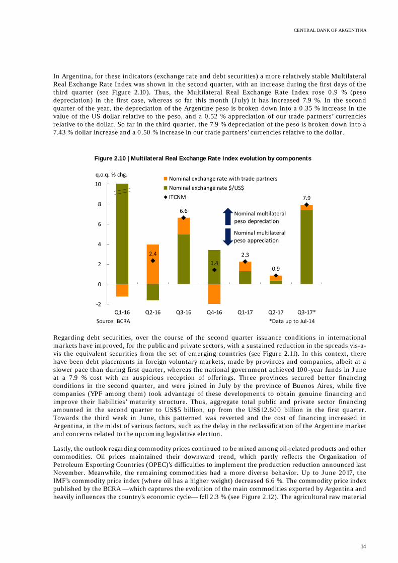
In Argentina, for these indicators (exchange rate and debt securities) a more relatively stable Multilateral Real Exchange Rate Index was shown in the second quarter, with an increase during the first days of the third quarter (see Figure 2.10). Thus, the Multilateral Real Exchange Rate Index rose 0.9 % (peso depreciation) in the first case, whereas so far this month (July) it has increased 7.9 %. In the second quarter of the year, the depreciation of the Argentine peso is broken down into a 0.35 % increase in the value of the US dollar relative to the peso, and a 0.52 % appreciation of our trade partners’ currencies relative to the dollar. So far in the third quarter, the 7.9 % depreciation of the peso is broken down into a 7.43 % dollar increase and a 0.50 % increase in our trade partners’ currencies relative to the dollar.
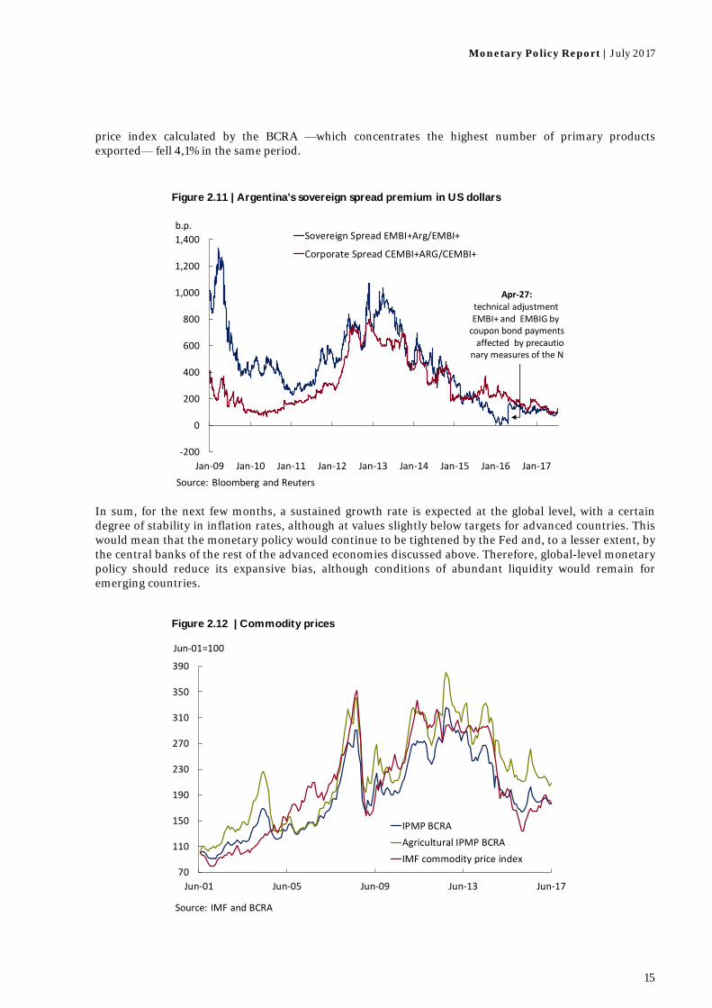
Regarding debt securities, over the course of the second quarter issuance conditions in international markets have improved, for the public and private sectors, with a sustained reduction in the spreads vis-a-vis the equivalent securities from the set of emerging countries (see Figure 2.11). In this context, there have been debt placements in foreign voluntary markets, made by provinces and companies, albeit at a slower pace than during first quarter, whereas the national government achieved 100-year funds in June at a 7.9 % cost with an auspicious reception of offerings. Three provinces secured better financing conditions in the second quarter, and were joined in July by the province of Buenos Aires, while five companies (YPF among them) took advantage of these developments to obtain genuine financing and improve their liabilities’ maturity structure. Thus, aggregate total public and private sector financing amounted in the second quarter to US$5 billion, up from the US$12.600 billion in the first quarter. Towards the third week in June, this patterned was reverted and the cost of financing increased in Argentina, in the midst of various factors, such as the delay in the reclassification of the Argentine market and concerns related to the upcoming legislative election.
Lastly, the outlook regarding commodity prices continued to be mixed among oil-related products and other commodities. Oil prices maintained their downward trend, which partly reflects the Organization of Petroleum Exporting Countries (OPEC)’s difficulties to implement the production reduction announced last November. Meanwhile, the remaining commodities had a more diverse behavior. Up to June 2017, the IMF’s commodity price index (where oil has a higher weight) decreased 6.6 %. The commodity price index published by the BCRA —which captures the evolution of the main commodities exported by Argentina and heavily influences the country’s economic cycle— fell 2.3 % (see Figure 2.12). The agricultural raw material
Figure 2.10 | Multilateral Real Exchange Rate Index evolution by components
2.4
6.6
1.4
2.3
0.9
7.9
‐2
0
2
4
6
8
10
Q1‐16 Q2‐16 Q3‐16 Q4‐16 Q1‐17 Q2‐17 Q3‐17*
q.o.q. % chg.Nominal exchange rate with trade partners
Nominal exchange rate $/US$
ITCNM
Source: BCRA *Data up to Jul‐14
Nominal multilateral peso depreciation
Nominal multilateral peso appreciation
Monetary Policy Report | July 2017
15
price index calculated by the BCRA —which concentrates the highest number of primary products exported— fell 4,1% in the same period.
In sum, for the next few months, a sustained growth rate is expected at the global level, with a certain degree of stability in inflation rates, although at values slightly below targets for advanced countries. This would mean that the monetary policy would continue to be tightened by the Fed and, to a lesser extent, by the central banks of the rest of the advanced economies discussed above. Therefore, global-level monetary policy should reduce its expansive bias, although conditions of abundant liquidity would remain for emerging countries.
Figure 2.11 | Argentina’s sovereign spread premium in US dollars
Figure 2.12 | Commodity prices
‐200
0
200
400
600
800
1,000
1,200
1,400
Jan‐09 Jan‐10 Jan‐11 Jan‐12 Jan‐13 Jan‐14 Jan‐15 Jan‐16 Jan‐17
Sovereign Spread EMBI+Arg/EMBI+
Corporate Spread CEMBI+ARG/CEMBI+
b.p.
Source: Bloomberg and Reuters
Apr‐27:technical adjustmentEMBI+ and EMBIG bycoupon bond paymentsaffected by precautio
nary measures of the N
70
110
150
190
230
270
310
350
390
Jun‐01 Jun‐05 Jun‐09 Jun‐13 Jun‐17
Jun‐01=100
IPMP BCRA
Agricultural IPMP BCRA
IMF commodity price index
Source: IMF and BCRA

CENTRAL BANK OF ARGENTINA
16
3. Economic Activity July marks 11 months after having overcome the recession started in September 2015. Since the fourth quarter in 2016, the GDP has expanded at an annual rate of 4 %.
The characteristics of this expansive phase have shared typical traits of growth cycles in other countries in the region. Internal expenditure components (consumption and investment) have accompanied GDP growth, showing higher variation rates. Net foreign flows have correlated inversely, with imports growing at a higher rate than exports.
The increase in GDP consolidates with more widespread growth among productive and higher-intensity sectors.
It is expected that these economic trends would strengthen in the forthcoming periods, reaching a 2.7 % growth for the year, according to the latest estimations drawn from the survey of market expectations (REM). For 2018 and 2019, the REM expects the economy to stay in its path, with a 3 % and 3.2 % growth, respectively.
3.1 Almost One Year After the End of the Recession
The economy has continued to strengthen9. June marked three quarters of growth at an annualized rate of around 4 % (see Figure 3.1). From January to March 2017, the GDP grew at a quarterly rate of 1.1 % (s.a.), thus exceeding the forecast of the previous IPOM (0.7 % s.a.) and in line with the REM’s expectations. During the second quarter, activity seems to have continued to expand, at a quarterly rate of 1 % according to the BCRA contemporary forecast for the GDP (PCP-BCRA; see Exhibit 2 / BCRA’s contemporary product forecast).
9 The level of activity is still below potential GDP — the one that may be reached keeping a constant inflation rate.
Figure 3.1 | Economic activity
138
141
144
147
150
153
May‐15 Aug‐15 Nov‐15 Feb‐16 May‐16 Aug‐16 Nov‐16 Feb‐17 May‐17
2004=100 EMAE s.a. EMAE t.c. IGA s.a. IGA t.c. GDP s.a.
Notes: s.a.: seasonally adjusted. t.c.: trend‐cycle. EMAE:monthly Economic Activity Indicator INDEC. IGA: General Activity Index released by Orlando J. Ferreres. PCP‐BCRA: BCRA Nowcast
PCP‐BCRAQ2‐17:+0.99%
+0.1%+0.7%
+1.1%
Monetary Policy Report | July 2017
17
3.2 What Can be Expected for the Expansive Phases of an Economic Cycle?
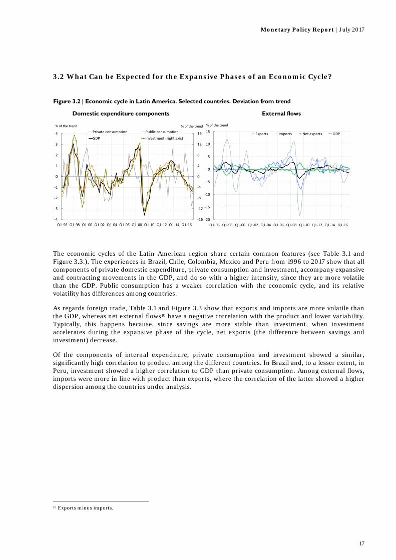
The economic cycles of the Latin American region share certain common features (see Table 3.1 and Figure 3.3.). The experiences in Brazil, Chile, Colombia, Mexico and Peru from 1996 to 2017 show that all components of private domestic expenditure, private consumption and investment, accompany expansive and contracting movements in the GDP, and do so with a higher intensity, since they are more volatile than the GDP. Public consumption has a weaker correlation with the economic cycle, and its relative volatility has differences among countries.
As regards foreign trade, Table 3.1 and Figure 3.3 show that exports and imports are more volatile than the GDP, whereas net external flows10 have a negative correlation with the product and lower variability. Typically, this happens because, since savings are more stable than investment, when investment accelerates during the expansive phase of the cycle, net exports (the difference between savings and investment) decrease.
Of the components of internal expenditure, private consumption and investment showed a similar, significantly high correlation to product among the different countries. In Brazil and, to a lesser extent, in Peru, investment showed a higher correlation to GDP than private consumption. Among external flows, imports were more in line with product than exports, where the correlation of the latter showed a higher dispersion among the countries under analysis.
10 Exports minus imports.
Figure 3.2 | Economic cycle in Latin America. Selected countries. Deviation from trend
Domestic expenditure components External flows
‐16
‐12
‐8
‐4
0
4
8
12
16
‐4
‐3
‐2
‐1
0
1
2
3
4
Q1‐96 Q1‐98 Q1‐00 Q1‐02 Q1‐04 Q1‐06 Q1‐08 Q1‐10 Q1‐12 Q1‐14 Q1‐16
Private consumption Public consumption
GDP Investment (right axis)
% of the trend% of the trend
‐20
‐15
‐10
‐5
0
5
10
15
Q1‐96 Q1‐98 Q1‐00 Q1‐02 Q1‐04 Q1‐06 Q1‐08 Q1‐10 Q1‐12 Q1‐14 Q1‐16
Exports Imports Net exports GDP
% of the trend

CENTRAL BANK OF ARGENTINA
18
‐18
‐15
‐12
‐9
‐6
‐3
0
3
6
9
12
‐12
‐10
‐8
‐6
‐4
‐2
0
2
4
6
8
Q1‐96 Q1‐98 Q1‐00 Q1‐02 Q1‐04 Q1‐06 Q1‐08 Q1‐10 Q1‐12 Q1‐14 Q1‐16
Private consumption Public consumption
GDP Investment (right axis)
% of the trend % of the trend
‐20
‐15
‐10
‐5
0
5
10
15
20
Q1‐96 Q1‐98 Q1‐00 Q1‐02 Q1‐04 Q1‐06 Q1‐08 Q1‐10 Q1‐12 Q1‐14 Q1‐16
Exports Imports
Net exports GDP
% of the trend
‐20
‐15
‐10
‐5
0
5
10
15
20
‐8
‐6
‐4
‐2
0
2
4
6
8
Q1‐96 Q1‐98 Q1‐00 Q1‐02 Q1‐04 Q1‐06 Q1‐08 Q1‐10 Q1‐12 Q1‐14 Q1‐16
% of the trend % of the trend
‐25
‐20
‐15
‐10
‐5
0
5
10
15
20
Q1‐96 Q1‐98 Q1‐00 Q1‐02 Q1‐04 Q1‐06 Q1‐08 Q1‐10 Q1‐12 Q1‐14 Q1‐16
% of the trend
‐45
‐30
‐15
0
15
30
45
60
75
‐6
‐4
‐2
0
2
4
6
8
10
Q1‐96 Q1‐98 Q1‐00 Q1‐02 Q1‐04 Q1‐06 Q1‐08 Q1‐10 Q1‐12 Q1‐14 Q1‐16
% of the trend % of the trend
‐20
‐15
‐10
‐5
0
5
10
15
20
Q1‐96 Q1‐98 Q1‐00 Q1‐02 Q1‐04 Q1‐06 Q1‐08 Q1‐10 Q1‐12 Q1‐14 Q1‐16
% of the trend
‐20
‐15
‐10
‐5
0
5
10
15
‐8
‐6
‐4
‐2
0
2
4
6
Q1‐96 Q1‐98 Q1‐00 Q1‐02 Q1‐04 Q1‐06 Q1‐08 Q1‐10 Q1‐12 Q1‐14 Q1‐16
% of the trend % of the trend
‐25
‐20
‐15
‐10
‐5
0
5
10
15
Q1‐96Q1‐98Q1‐00Q1‐02Q1‐04Q1‐06Q1‐08Q1‐10Q1‐12Q1‐14Q1‐16
% of the trend
‐30
‐15
0
15
30
45
‐10
‐5
0
5
10
15
Q1‐96 Q1‐98 Q1‐00 Q1‐02 Q1‐04 Q1‐06 Q1‐08 Q1‐10 Q1‐12 Q1‐14 Q1‐16
% of the trend % of the trend
‐20
‐15
‐10
‐5
0
5
10
15
20
Q1‐96Q1‐98Q1‐00Q1‐02Q1‐04Q1‐06Q1‐08Q1‐10Q1‐12Q1‐14Q1‐16
% of the trend
Figure 3.3 | Economic cycle. Selected countries. Deviation from trend
Brazil
Chile
Colombia
Mexico
Peru

Monetary Policy Report | July 2017
19
3.3 The Growth Phase in the Argentine Cycle
The Argentine experience is in line with the observations made for the region. Both investment and exports have showed even a higher correlation to GDP than its Latin American peers. Notoriously, while exports’ and private consumption’s variability matches the median for the rest of the economies, and investment, public consumption and imports have relatively low volatility, the GDP is the most volatile in the region (see Table 3.1).
3.3.1 Unlike Other Cycles, Exports’ Recovery Preceded GDP Growth
Since the onset of the economic recovery to the end of the first quarter of 2017, external sales grew 7.4 %, thus exceeding growth in the components of domestic expenditure. Exports have even rallied in the recessive phase of the cycle, owing to the elimination of the pervasive foreign exchange controls (cepo cambiario) and the tax reduction, which distinguished the country’s experience from that of its neighbors and its own history (see Figure 3.4).
Although there are signs that exports may have temporarily stopped growing in the second quarter, they are expected to resume their growing path in the second half of the year. On one hand, producers should start shipping corn once again, after the interruptions caused by weather conditions in the first half of the year, while soy product sales should become more dynamic as prices in local currency increase their appeal11. Also, industrial manufactured exports should maintain the growth trend they initiated in mid-2016, with a growing contribution from Brazil.
11 External sales of soy products in the second quarter were impacted by the holdup of soy beans by local producers waiting for better internal price. The internal price depends on the evolution of international prices and the exchange rate.
Table 3.1 | Empirical regularity in cycles. Selected countries.
Standard deviation
GDP correlations vs. variables
Private consumption Public consumption Investment Exports Imports Net exports
Brasil 1.60 1.13 1.11 2.93 2.67 4.77 0.51
Chile 1.80 1.26 0.75 3.58 1.68 3.79 0.85
Colombia 1.62 0.99 1.77 6.11 2.26 4.41 0.82
México 2.23 1.14 0.64 3.42 2.07 3.17 0.51
Perú 2.12 1.18 2.26 5.67 2.12 3.31 0.79
Argentina 2.89 1.14 0.47 2.94 1.93 3.08 0.49
Avg. 6 countries 2.04 1.14 1.17 4.11 2.12 3.75 0.66
Country GDP deviation (%)Std. Deviation relative to GDP
Country Private consumption Public consumption Investment Exports Imports Net exports
Brazil 0.74 0.20 0.87 0.35 0.72 ‐0.60
Chile 0.94 0.10 0.84 0.61 0.85 ‐0.54
Colombia 0.90 0.46 0.81 0.30 0.86 ‐0.75
Mexico 0.93 0.50 0.90 0.42 0.93 ‐0.68
Peru 0.68 0.10 0.69 0.32 0.72 ‐0.43
Argentina 0.90 0.28 0.94 0.70 0.87 ‐0.55
Avg. 6 countries 0.85 0.27 0.84 0.45 0.82 ‐0.59
CENTRAL BANK OF ARGENTINA
20
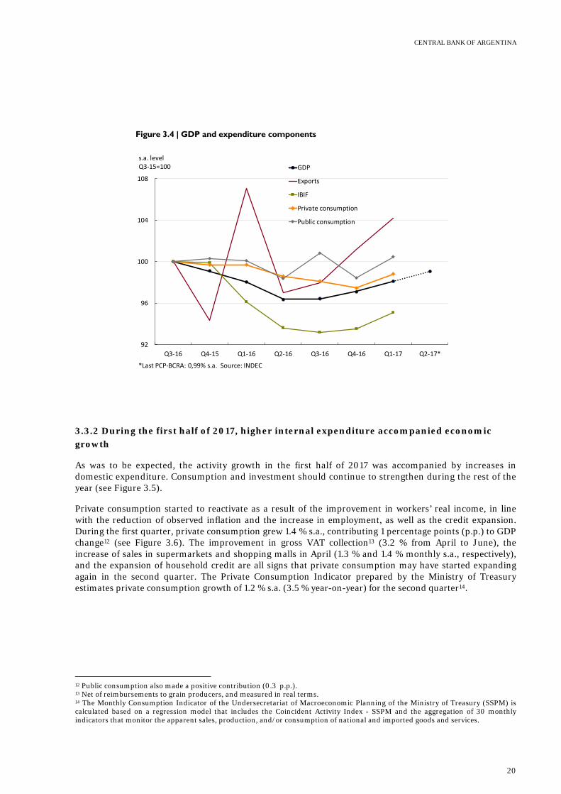
3.3.2 During the first half of 2017, higher internal expenditure accompanied economic growth
As was to be expected, the activity growth in the first half of 2017 was accompanied by increases in domestic expenditure. Consumption and investment should continue to strengthen during the rest of the year (see Figure 3.5).
Private consumption started to reactivate as a result of the improvement in workers’ real income, in line with the reduction of observed inflation and the increase in employment, as well as the credit expansion. During the first quarter, private consumption grew 1.4 % s.a., contributing 1 percentage points (p.p.) to GDP change12 (see Figure 3.6). The improvement in gross VAT collection13 (3.2 % from April to June), the increase of sales in supermarkets and shopping malls in April (1.3 % and 1.4 % monthly s.a., respectively), and the expansion of household credit are all signs that private consumption may have started expanding again in the second quarter. The Private Consumption Indicator prepared by the Ministry of Treasury estimates private consumption growth of 1.2 % s.a. (3.5 % year-on-year) for the second quarter14.
12 Public consumption also made a positive contribution (0.3 p.p.). 13 Net of reimbursements to grain producers, and measured in real terms. 14 The Monthly Consumption Indicator of the Undersecretariat of Macroeconomic Planning of the Ministry of Treasury (SSPM) is calculated based on a regression model that includes the Coincident Activity Index - SSPM and the aggregation of 30 monthly indicators that monitor the apparent sales, production, and/or consumption of national and imported goods and services.
Figure 3.4 | GDP and expenditure components
92
96
100
104
108
Q3‐16 Q4‐15 Q1‐16 Q2‐16 Q3‐16 Q4‐16 Q1‐17 Q2‐17*
s.a. levelQ3‐15=100 GDP
Exports
IBIF
Private consumption
Public consumption
*Last PCP‐BCRA: 0,99% s.a. Source: INDEC
Monetary Policy Report | July 2017
21
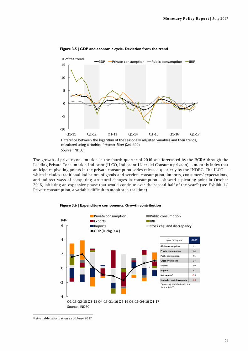
The growth of private consumption in the fourth quarter of 2016 was forecasted by the BCRA through the Leading Private Consumption Indicator (ILCO, Indicador Lider del Consumo privado), a monthly index that anticipates pivoting points in the private consumption series released quarterly by the INDEC. The ILCO —which includes traditional indicators of goods and services consumption, imports, consumers’ expectations, and indirect ways of computing structural changes in consumption— showed a pivoting point in October 2016, initiating an expansive phase that would continue over the second half of the year15 (see Exhibit 1 / Private consumption, a variable difficult to monitor in real time).
15 Available information as of June 2017.
Figure 3.5 | GDP and economic cycle. Deviation from the trend
Figure 3.6 | Expenditure components. Growth contribution
‐10
‐5
0
5
10
15
Q1‐11 Q1‐12 Q1‐13 Q1‐14 Q1‐15 Q1‐16 Q1‐17
% of the trendGDP Private consumption Public consumption IBIF
Source: INDEC
Difference between the logarithm of the seasonally adjusted variables and their trends, calculated using a Hodrick‐Prescott filter (λ=1.600)
‐4
‐2
0
2
4
6
Q1‐15 Q2‐15 Q3‐15 Q4‐15 Q1‐16 Q2‐16 Q3‐16 Q4‐16 Q1‐17
Private consumption Public consumption
Exports IBIF
Imports stock chg. and discrepancy
GDP (% chg. s.a.)
p.p.
Source: INDEC
GDP constant prices 1.1
Private consumption 1.4
Public consumption 2.1
Gross investment 1.7
Exports 2.9
Imports 3.2
Net exports* ‐0.3
Stock chg. and discrepancy ‐0.3
Source: INDEC
*q.o.q. chg. contribution in p.p.
Q1‐17q.o.q. % chg. s.a.

CENTRAL BANK OF ARGENTINA
22
Gross domestic investment continued to rally, in line with the expansive phase of the cycle. It grew 1.7 % s.a. in the first quarter and, according to several indicators, it would grew again in April and June. Public works accounted for most of the behavior of construction activity in the first half of the year. Asphalt orders for road works were among the historical records, with an 83 % increase year-on-year in June 2017. Based on the infrastructure projects tendered in the last year, and in line with the expansion expected in the 2017 budget, public works should stay dynamic for the next few months (see Figure 3.7).
During the second quarter, private investment also joined this trend with more momentum, with signs of reactivation both in the construction and the durable production equipment segments. Within construction, bagged cement sales were strongly dynamic, and there was an important increase in the Construya Index, which captures mainly the categories related to private building construction completion. The outlook of the private building construction sector is mostly optimistic16, and the sector will also be benefited by the BCRA’s enabling of financial entities to accept Preliminary sales contract and construction trust fund shares as collateral for UVA-denominated mortgage loans17. The rise in real expenditure in the durable production equipment was translated into a strong increase of imported quantities and a more moderate rise in demand for domestic equipment. Based on FIEL’s capital goods imports and industrial production data, an increase in investment in the durable production equipment is to be expected for the second quarter (see Figure 3.8).
16 52.6 percent of respondents expect their activity to increase between June and August, above the share expecting it to remain unchanged (42.1 percent). INDEC, Indicadores de coyuntura de la actividad de la construcción. May 2017. Vol. 1 N° 6. 17 This is coupled by increasing funding in UVA mortgage loans. During the second quarter, financial entities granted $8,667 million in UVA loans, 63.6 percent of which were mortgage loans.
Figure 3.7 | Investment in construction
75
85
95
105
115
125
Jun‐14 Jun‐15 Jun‐16 Jun‐17
s.a. 2011=100
Total cement dispatches todomestic marketConstruya Index
30
50
70
90
110
130
May‐14 Nov‐15 May‐17
Asphalt
Bulk cement dispatches
Capital expenditure
s.a. 2011=100
*Real direct investment and capital transfers to the non‐financial national public sector deflated by Construction Cost Index Source: INDEC, Treasury Secretariat, AFCP and Ministry of Energy and Mines
Monetary Policy Report | July 2017
23
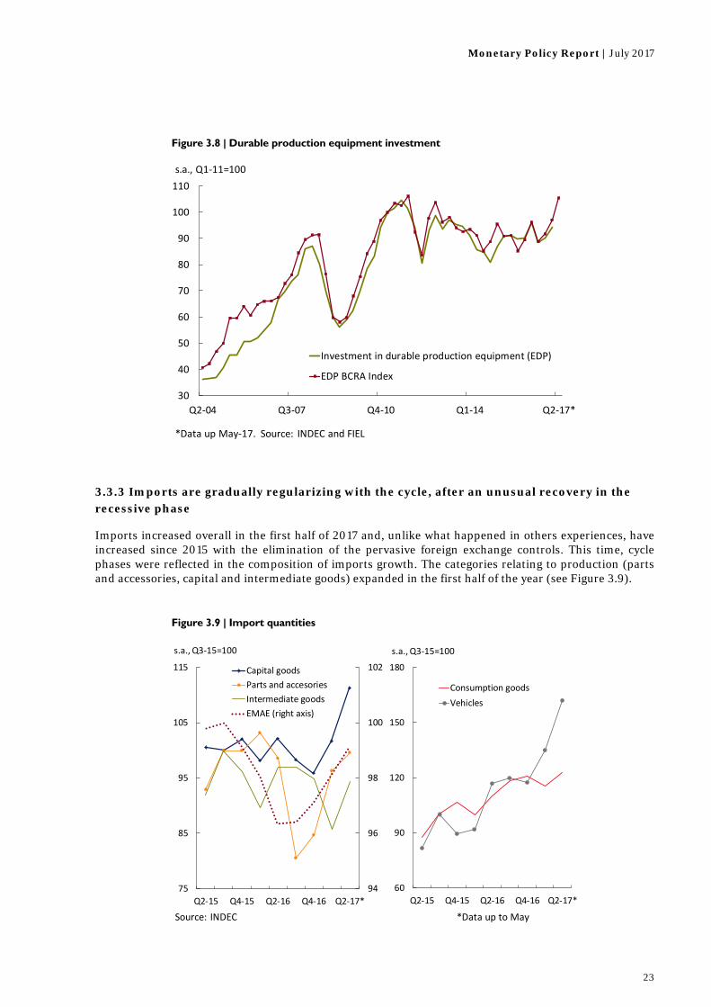
3.3.3 Imports are gradually regularizing with the cycle, after an unusual recovery in the recessive phase
Imports increased overall in the first half of 2017 and, unlike what happened in others experiences, have increased since 2015 with the elimination of the pervasive foreign exchange controls. This time, cycle phases were reflected in the composition of imports growth. The categories relating to production (parts and accessories, capital and intermediate goods) expanded in the first half of the year (see Figure 3.9).
Figure 3.8 | Durable production equipment investment
Figure 3.9 | Import quantities
30
40
50
60
70
80
90
100
110
Q2‐04 Q3‐07 Q4‐10 Q1‐14 Q2‐17*
Investment in durable production equipment (EDP)
EDP BCRA Index
*Data up May‐17. Source: INDEC and FIEL
s.a., Q1‐11=100
94
96
98
100
102
75
85
95
105
115
Q2‐15 Q4‐15 Q2‐16 Q4‐16 Q2‐17*
s.a., Q3‐15=100s.a., Q3‐15=100
Capital goods
Parts and accesories
Intermediate goods
EMAE (right axis)
Source: INDEC *Data up to May
60
90
120
150
180
Q2‐15 Q4‐15 Q2‐16 Q4‐16 Q2‐17*
Consumption goods
Vehicles
CENTRAL BANK OF ARGENTINA
24
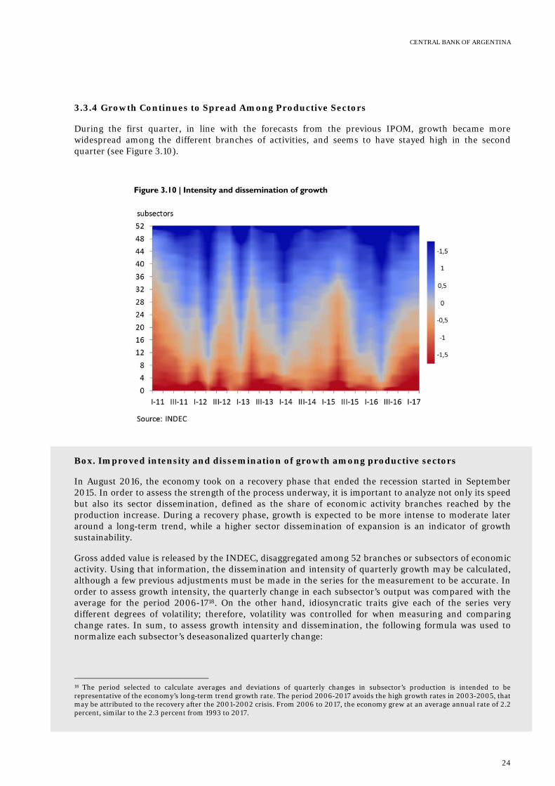
3.3.4 Growth Continues to Spread Among Productive Sectors
During the first quarter, in line with the forecasts from the previous IPOM, growth became more widespread among the different branches of activities, and seems to have stayed high in the second quarter (see Figure 3.10).
Box. Improved intensity and dissemination of growth among productive sectors
In August 2016, the economy took on a recovery phase that ended the recession started in September 2015. In order to assess the strength of the process underway, it is important to analyze not only its speed but also its sector dissemination, defined as the share of economic activity branches reached by the production increase. During a recovery phase, growth is expected to be more intense to moderate later around a long-term trend, while a higher sector dissemination of expansion is an indicator of growth sustainability.
Gross added value is released by the INDEC, disaggregated among 52 branches or subsectors of economic activity. Using that information, the dissemination and intensity of quarterly growth may be calculated, although a few previous adjustments must be made in the series for the measurement to be accurate. In order to assess growth intensity, the quarterly change in each subsector’s output was compared with the average for the period 2006-1718. On the other hand, idiosyncratic traits give each of the series very different degrees of volatility; therefore, volatility was controlled for when measuring and comparing change rates. In sum, to assess growth intensity and dissemination, the following formula was used to normalize each subsector’s deseasonalized quarterly change:
18 The period selected to calculate averages and deviations of quarterly changes in subsector’s production is intended to be representative of the economy’s long-term trend growth rate. The period 2006-2017 avoids the high growth rates in 2003-2005, that may be attributed to the recovery after the 2001-2002 crisis. From 2006 to 2017, the economy grew at an average annual rate of 2.2 percent, similar to the 2.3 percent from 1993 to 2017.
Figure 3.10 | Intensity and dissemination of growth

Monetary Policy Report | July 2017
25
= normalized quarterly change i
= quarterly change i
= 2006-2017 average quarterly change
= standard deviation of quarterly change
The standardized quarterly change of the 52 subsectors of activity is listed from lower to higher standardized growth in a heatmap. The higher the quarterly increase (fall), the more intense the red (blue) subsectors were illustrated with.
The figure shows that the number of activity branches growing around or above their mean has gradually increased, together with the intensity of their growth (see Figure 3.10). In the first quarter of 2017, 51.9 % (27) of subsectors grew at a rate above their mean, while in the second quarter of 2016 only 5.8 % (3) did so with a higher intensity.
The set of policies adopted since late 201519 have started to come to fruition in terms of economic growth and have been reflected in the sectors that have led the economic recovery. Among them is the agricultural sector, which anticipated the GDP recovery, construction, real estate, transport and communications, and financial intermediation. Other, more moderately growing groups, such as hotels and restaurants, and other basic services, such as education and health, have accompanied the cycle. Lastly, industry and commerce also show signs of reactivation, albeit weakly for now (see Figure 3.11).
19 The policies implemented include the elimination of exchange restrictions, the lowering and elimination of duties on exports, the elimination of exports quotas and records, the end of the default, which allowed the public and private sectors to access international financial markets, the implementation of the inflation targeting regime, the deregulation of interest rates, and the UVA credits.
Figure 3.11 | GDP. Main productive sectors
80
85
90
95
100
105
Q1‐15 Q4‐15 Q3‐16 Q2‐17e
s.a. 2015=100
Real estate activities
Financial intermediation
Construction88
92
96
100
104
Q1‐15 Q4‐15 Q3‐16 Q2‐17e
Industry
Commerce
s.a. 2015=100
Note: Q2‐17 has been estimated with ARIMA models, using as determinants the available leading indicators.Source: INDEC, BCRA, AFCP, Notary College of CABA and Buenos Aires province, FIEL and O.J. Ferreres

CENTRAL BANK OF ARGENTINA
26
In another aspect of this expansive phase, total formal employment grew 1 % in April 2017 relative to last year. Private sector job creation accounted for 70 % of this increase20 (73,400 workers), unlike the previous period of employment expansion (Dec/14-Oct/15), when total employment evolution was largely due to the increase in public employment (54 %)21 (see Figure 3.12). The number of workers in the formal private sector offset the fall recorded during the contraction phase, and is now slightly above regarding October 2015.
According to the INDEC, labor supply during the period —as measured by the activity rate— exceeded the increase in demand, which led the unemployment rate to rise to 9.2 %. The outlook for the next three months is optimistic, based on the job creation expectations of the Labor Market Indicators Survey (EIL Encuesta de Indicadores Laborales) of the Ministry of Labor, Employment and Social Security from last May.
The private employment growth rate is expected to be lower than product growth in the onset of an expansion phase, which shows a rise in productivity per worker22. During the contraction phase, companies often operate underusing the labor factor through suspensions and/or working hours reductions. In the onset of a recovery of economic activity, firms tend to normalize underuse before deciding on a staff expansion. Economic reforms aimed at increasing productivity will encourage job creation and an improvement in real wages (see Figure 3.13).
20 Excluding self-employee. 21During the last year (April 17-April 16), 69 percent of the evolution of total formal employment was accounted for by private sector job creation, whereas public employment accounted for 31 percent. In contrast, during the previous expansion (December 14-October 15), public employment represented 54 percent of employment change, while the private sector contributed 46 percent. 22 In the onset of an expansive phase, the higher flexibility of work hours relative to jobs creates more intense growth in product per job than in productivity per hour.
Figure 3.12 | Employment and activity
97
98
99
100
101
102
103
104
‐60
‐40
‐20
0
20
40
60
80
100
120
140
Aug‐15 Dec‐15 Apr‐16 Aug‐16 Dec‐16 Apr‐17
accum. chg. Apr‐16=0
Public sector employment
Total employment
Private employment
EMAE (right axis)
Apr‐16=100
Source: INDEC and Ministry of Labor, Employment and Social Security

Monetary Policy Report | July 2017
27
3.3.5 Real Wages and the Relative Price of Nontradable Goods and Services Improve, along with the Expansive Phase of the Cycle
The recovery process of real wages in the formal private sector, that had begun in the second half of last year, continued during the second quarter, in context of GDP improvement and lower rates of price increase (see Figure 3.14).
Figure 3.13 | Private employment, activity and real wages. Deviation from the trend
Figure 3.14 | GDP and real wage. Deviation from the trend
‐10
‐8
‐5
‐3
0
3
5
Apr‐09 Apr‐10 Apr‐11 Apr‐12 Apr‐13 Apr‐14 Apr‐15 Apr‐16 Apr‐17
% of trend
EMAE/total private employment ratio
EMAE
Private sector total employment
Deflated wages
Note: Difference between the logarithm of the seasonally adjusted variables and their trends, calculated using a Hodrick‐Prescott filter (λ = 1,600).Source: INDEC, AFIP and Ministry of Labor, Employment and Social Security
‐6
‐5
‐4
‐3
‐2
‐1
0
1
2
3
4
III‐12 II‐13 I‐14 IV‐14 III‐15 II‐16 I‐17
GDP Real wage
% of trend
Difference between the logarithm of the seasonally adjusted variables and their trends, calculated using a Hodrick‐Prescott filter (λ=1.600) Source: INDEC, AFIP and Statistical offices of City of Buenos Aires, San Luis and Córdoba
CENTRAL BANK OF ARGENTINA
28
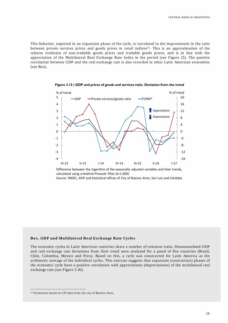
This behavior, expected in an expansion phase of the cycle, is correlated to the improvement in the ratio between private services prices and goods prices in retail indices23. This is an approximation of the relative evolution of non-tradable goods prices and tradable goods prices, and is in line with the appreciation of the Multilateral Real Exchange Rate Index in the period (see Figure 15). The positive correlation between GDP and the real exchange rate is also recorded in other Latin American economies (see Box).
Box. GDP and Multilateral Real Exchange Rate Cycles
The economic cycles in Latin American countries share a number of common traits. Deseasonalized GDP and real exchange rate deviations from their trend were analyzed for a panel of five countries (Brazil, Chile, Colombia, Mexico and Peru). Based on this, a cycle was constructed for Latin America as the arithmetic average of the individual cycles. This exercise suggests that expansion (contraction) phases of the economic cycle have a positive correlation with appreciations (depreciations) of the multilateral real exchange rate (see Figure 3.16).
23 Estimation based on CPI data from the city of Buenos Aires.
Figure 3.15 | GDP and prices of goods and services ratio. Deviation from the trend
‐16
‐12
‐8
‐4
0
4
8
12
16
20
‐4
‐3
‐2
‐1
0
1
2
3
4
5
III‐12 II‐13 I‐14 IV‐14 III‐15 II‐16 I‐17
GDP Private services/goods ratio ITCRM*
% of trend % of trend
Appreciation
Depreciation
Difference between the logarithm of the seasonally adjusted variables and their trends, calculated using a Hodrick‐Prescott filter (λ=1.600)Source: INDEC, AFIP and Statistical offices of City of Buenos Aires, San Luis and Córdoba

Monetary Policy Report | July 2017
29
3.4 Outlook: On the Right Path, With Room for Further Growth
The new macroeconomic setting implemented jointly with the correction of relative prices, the tax reduction and the elimination of distortions that hindered the economy has triggered widespread, increasingly intense growth.
For the next few quarters, the BCRA expects the economy to continue on the expansion phase started during the third quarter of 2016. This expectation is in line with the Survey of Market Expectations, who projected 4 % annualized growth rates for the third and fourth quarters of 2017 (see Figure 3.17).
Growth should continue to spread among the different sectors, fueling job creation. Exports will resume their positive trend in the second half of the year, driven by the sale of the record crop in the agricultural sector and the recovery of demand from Brazil. Domestic expenditure components should continue to accompany the product expansion phase, as usual, together with real wages.
Figure 3.16 | Latin America. Selected countries. GDP and Real Multilateral Exchange Rate (dollar/currency). Deviation from trend
Figure 3.17 | REM growth forecasts
‐5
‐4
‐3
‐2
‐1
0
1
2
3
4
‐25
‐20
‐15
‐10
‐5
0
5
10
15
20
I‐97
II‐98
III‐99
IV‐00
I‐02
II‐03
III‐04
IV‐05
I‐07
II‐08
III‐09
IV‐10
I‐12
II‐13
III‐14
IV‐15
I‐17
Real Multilateral Exchange Rate (US$/currency)
GDP* (right axis)
*Corresponds to the GDP of the set of countries (Brazil, Chile,Colombia, Mexico and Peru). Difference between the logarithmof the seasonally adjusted variable and its trend, calculated witha Hodrick‐Prescott filter (λ = 1,600). For the Real Exchange Rate,the deviation from the linear trend was considered. Source:Official bodies of the Institutes of Statistics and Bruegel
% deviation from trend % deviation from trend
Appreciation
Depreciation
1.0 1.0 1.0
2.73.0
3.2
‐1.1
‐1.7
0.1
0.71.1
‐2.0
‐1.0
‐
1.0
2.0
3.0
4.0
Q1‐16 Q2‐16 Q3‐16 Q4‐16 Q1‐17 Q2‐17 Q3‐17 Q4‐17 2017 2018 2019
% chg.
REM Dec‐16
REM Mar‐17
REM Jun‐17
Quarterly data s.a.
Source: REM ‐ BCRA Q2‐17 annual implicit forecast
annualq.o.q. s.a.
Country
Correlation
coefficient
with cycles
Brazil 0.29
Chile 0.35
Colombia 0.31
Mexico 0.26
Peru 0.22

CENTRAL BANK OF ARGENTINA
30
Exhibit 1 / Private consumption, a difficult variable to monitor in real time In the BCRA’s monitoring of the current scenario, private consumption is one of the most interesting, and also one of the most complex, variables. As a result of the many consumption indicators that offer valuable (albeit partial or incomplete) information as they are published, these must be analyzed always within a wider set of informative variables for them to acquire relevant predictive value for private consumption.
The aim is to create leading consumption indicators or simply predict consumption behavior by means of proxy variables related to private consumption, published before quarterly national accounts. Typically, market analysts link private consumption only to the demand for goods (supermarket, retail, and shopping mall sales; car or house appliances sales) without taking into account that services (such as transport, housing, health, education, recreation, etc.) have a significant share in households’ consumption expenditure. In 2016, service consumption accounted for around 60 % of total private consumption, whereas goods barely represented 40 %.24
For these reasons, analyzing private consumption based on a single indicator, such as supermarket sales, besides representing only one part of total consumption, can create mixed, incomplete, partial signs that should not be generalized without taking into account a composite indicator involving a wider range of representative consumption indicators.
On the other hand, the changes in agents’ consumption habits, which are both circumstantial and structural, create challenges for traditional models and decrease their predictive power. In particular, the increased use of alternative or wholesale sales channels to the detriment of traditional outlets, such as supermarkets; or the gradual but irreversible changes in consumption patterns, such as the irruption of electronic commerce25, must be acknowledged to accurately model and forecast private consumption.
Bearing these considerations in mind and controlling for the seasonal effects, irregularities and volatility in the original series, the methodology used for the Leading Private Consumption Index (ILCO, Indicador Lider de Consumo Privado) was replicated (see IPOM January 2017) in order to identify pivoting points in the series and better anticipate policy and shock impact on consumption.
This indicator is made of variables26 that reflect traditional consumption measures for goods and services and imports, as well as indirect ways to compute structural changes in consumption. Lastly, an expectations variable is included, together with one reflecting growth diffusion for the whole variable set. Variables representing consumed quantities month on month are deseasonalized and receive a special treatment in order to minimize volatility.
A simple comparison between the partial indicators frequently used as consumption predictors and a more comprehensive one —in this case, the ILCO— indicates that the former are less accurate in monitoring the variable. The following table shows the correlation between these indicators and private consumption in the national accounts, once seasonal and irregular elements are eliminated from the series. As can be seen, the only one with a correlation above 80 % is the comprehensive ILCO indicator.
24 For more detail, see http://www.indec.gov.ar/uploads/gacetillasdeprensa/gacetilla_consumption_privado_05_17.pdf. 25 According to the data published by the Argentine Chamber of Electronic Commerce (CACE, Cámara Argentina de Comercio Electrónico), sales through this kind of channels accounted for 40 billion pesos in 2014, 68 billion in 2015, and 102 billion in 2016. 26 The indicator comprises the following variables: supermarket sales, shopping mall sales, real gross VAT, national car sales. Credit flows with cards, service imports, tourism, travel and tickets, personal loan flows, CCI CABA, consumption goods imports, commerce, hotels and restaurants.

Monetary Policy Report | July 2017
31
What does the ILCO have to say then of private consumption in the present economic situation? We know that, in the sample period 2004-17, the leading consumption indicator identified the turning points in the private consumption series two quarters ahead once, one quarter ahead three times, and in the same quarter twice (see Figure 1). In the third quarter of 2016, the ILCO signaled a turning point that effectively occurred in the following quarter. Last, for the second quarter of 2017, the ILCO forecasts that private consumption will continue to show positive signs.
Table 1 | Correlation with trend-cycle of private consumption
Figure 1 | Leading Private Consumption Index
Variable Coefficient
Supermarkets 45%
Car sales 47%
Shoppings 52%
VAT 69%
Leading indicator 85%
Source: INDEC, Treasury Secretariat, ADEFA, UTDT and BCRA
250
300
350
400
450
500
550
90
110
130
150
170
190
210
Q1‐04
Q3‐04
Q1‐05
Q3‐05
Q1‐06
Q3‐06
Q1‐07
Q3‐07
Q1‐08
Q3‐08
Q1‐09
Q3‐09
Q1‐10
Q3‐10
Q1‐11
Q3‐11
Q1‐12
Q3‐12
Q1‐13
Q3‐13
Q1‐14
Q3‐14
Q1‐15
Q3‐15
Q1‐16
Q3‐16
Q1‐17
Mar‐94=100
Leading consumption index
Private consumption (right axis)
billion $ of 2004
0
‐1
0‐1
0‐1
+1‐2
f: Forecast. Source: INDEC, Treasury Secretariat, ADEFA, UTDT and BCRA
Q2‐17f
CENTRAL BANK OF ARGENTINA
32
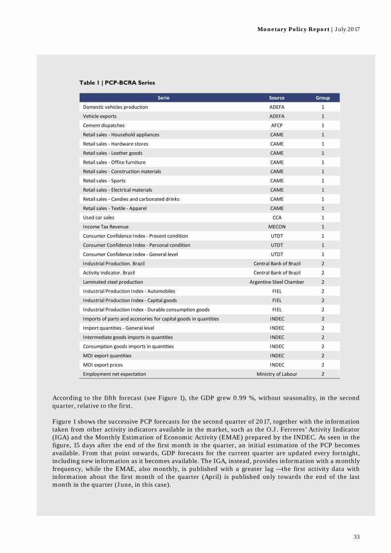
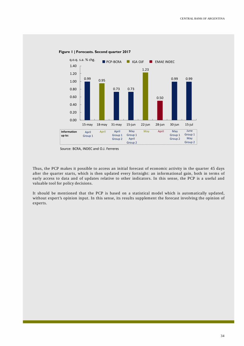
Exhibit 2 / BCRA’s contemporary product forecast Starting in the second quarter of 2017, the BCRA’s contemporary product forecast (PCP-BCRA) includes a greater number of economic indicators in order to capture the dynamics of a wider range of sectors in the economy. According to the PCP, with data as of July 15, the GDP grew 0.99 %, without seasonality, in the second quarter relative to the first. The PCP makes it possible to leverage the wealth of information from a large number of indicators published more frequently than the GDP in order to elaborate product forecasts within the quarter. Thus, it is possible to have access, 45 days after the start of the quarter, to leading estimations of the GDP figure, which is usually published approximately 10 weeks after the end of the quarter. Recently, new series were considered to be included in the PCP and thus achieve a greater coverage in terms of sectors of the economy. This process initially considered a broad set of cycle indicators (116 in total) with potential to be used. They included “hard” indicators (so labeled because they convey rather accurate signals about the economy’s performance) —industrial production, construction activity, commerce, employment, foreign trade, and Brazilian monetary, financial, fiscal and activity variables—, as well as “soft” indicators, seen as less accurate but providing valuable information about the perception of various economic agents as regards current and future conditions in the economy —employment expectation surveys, consumer confidence, among others. The criterion used to select the series to be included in the PCP was the existence of a significant contemporary correlation between the growth rate of each variable and the growth rate of activity (GDP). As a result, 30 series were chosen from the initial potential set (see Table 1). The methodology used to obtain the PCP, which is the same used in previous estimations, implies estimating the factors common to the set of indicators for the selected cycle and using those factors to predict the growth of GDP. The idea underlying this methodology is that the shared dynamics of the variables of interest can be explained by a reduced number of unobservable factors which account for the economy’s cyclical behavior. This set of 30 series was used to estimate the factors and, based on them, a model for the variation of the GDP. It was found that the first two factors account for 99% of the joint variability of the indicators at hand. Finally, the new factor model’s predictive power was compared to that of the one using a smaller set of series, based on both models’ forecast errors. It was found that the predictive power improves with the new set of data in 70% of the cases —44% in 2012–15 and 92 % starting in 2016. Having chosen the model, forecasts are updated as new information becomes available. To that effect, two groups of indicators are considered (Group 1 and Group 2), depending on the speed with which new data are available for the update (every fortnight), which makes it possible to produce 6 forecasts of activity in each quarter.
Monetary Policy Report | July 2017
33
According to the fifth forecast (see Figure 1), the GDP grew 0.99 %, without seasonality, in the second quarter, relative to the first. Figure 1 shows the successive PCP forecasts for the second quarter of 2017, together with the information taken from other activity indicators available in the market, such as the O.J. Ferreres’ Activity Indicator (IGA) and the Monthly Estimation of Economic Activity (EMAE) prepared by the INDEC. As seen in the figure, 15 days after the end of the first month in the quarter, an initial estimation of the PCP becomes available. From that point onwards, GDP forecasts for the current quarter are updated every fortnight, including new information as it becomes available. The IGA, instead, provides information with a monthly frequency, while the EMAE, also monthly, is published with a greater lag —the first activity data with information about the first month of the quarter (April) is published only towards the end of the last month in the quarter (June, in this case).
Table 1 | PCP-BCRA Series
Serie Source Group
Domestic vehicles production ADEFA 1
Vehicle exports ADEFA 1
Cement dispatches AFCP 1
Retail sales ‐ Household appliances CAME 1
Retail sales ‐ Hardware stores CAME 1
Retail sales ‐ Leather goods CAME 1
Retail sales ‐ Office furniture CAME 1
Retail sales ‐ Construction materials CAME 1
Retail sales ‐ Sports CAME 1
Retail sales ‐ Electrical materials CAME 1
Retail sales ‐ Candies and carbonated drinks CAME 1
Retail sales ‐ Textile ‐ Apparel CAME 1
Used car sales CCA 1
Income Tax Revenue MECON 1
Consumer Confidence Index ‐ Present condition UTDT 1
Consumer Confidence Index ‐ Personal condition UTDT 1
Consumer Confidence Index ‐ General level UTDT 1
Industrial Production. Brazil Central Bank of Brazil 2
Activity indicator. Brazil Central Bank of Brazil 2
Laminated steel production Argentine Steel Chamber 2
Industrial Production Index ‐ Automobiles FIEL 2
Industrial Production Index ‐ Capital goods FIEL 2
Industrial Production Index ‐ Durable consumption goods FIEL 2
Imports of parts and accesories for capital goods in quantities INDEC 2
Import quantities ‐ General level INDEC 2
Intermediate goods imports in quantities INDEC 2
Consumption goods imports in quantities INDEC 2
MOI export quantities INDEC 2
MOI export prices INDEC 2
Employment net expectation Ministry of Labour 2
CENTRAL BANK OF ARGENTINA
34
Thus, the PCP makes it possible to access an initial forecast of economic activity in the quarter 45 days after the quarter starts, which is then updated every fortnight: an informational gain, both in terms of early access to data and of updates relative to other indicators. In this sense, the PCP is a useful and valuable tool for policy decisions. It should be mentioned that the PCP is based on a statistical model which is automatically updated, without expert’s opinion input. In this sense, its results supplement the forecast involving the opinion of experts.
Figure 1 | Forecasts. Second quarter 2017
0.99 0.95
0.73 0.73
1.23
0.50
0.99 0.99
0.00
0.20
0.40
0.60
0.80
1.00
1.20
1.40
15‐may 18‐may 31‐may 15‐jun 22‐jun 28‐jun 30‐jun 15‐jul
q.o.q. s.a. % chg.PCP‐BCRA IGA OJF EMAE INDEC
AprilGroup 1
AprilGroup 1Group 2
MayGroup 1April
Group 2
MayGroup 1Group 2
JuneGroup 1May
Group 2
April May AprilInformationup to:
Source: BCRA, INDEC and O.J. Ferreres

Monetary Policy Report | July 2017
35
4. Prices The second quarter saw a further deceleration of inflation in year-on-year terms, reflecting the continuation of the disinflation process prevalent since mid-2016. In June, 2017, retail prices reached a year-on-year rate of increase of 22 %, the lowest since 2009. Inflation in the second quarter of the year was below of the period January-March. Having said that, core inflation showed some persistence in 2017, above the levels pretended by the monetary authority. Core inflation behavior is related to the dynamics of both goods and private services. The recovery of services relative to goods continued, both private and public. The expectations of the analysts of the Market Expectations Survey (REM) remained virtually unchanged relative to the survey included in the last Monetary Policy Report. In this scenario, the BCRA will keep a clear anti-inflation bias to ensure that the disinflation process continues on its path towards the target of 12 %-17 % for 2017, as well as an inflation rate at the end of 2017 compatible with the target of 10 % ± 2 % for 2018. 4.1 Inflation Resumed its Deceleration Path During the second quarter, inflation slowed down in year-on-year terms, reflecting the disinflation process prevalent since mid-2016. The various official retail indicators grew at a year-on-year rate of 22 %, the lowest since 200927. This price behavior took place during a strong reconfiguration of the relative prices of public utilities (see Figure 4.1). Wholesale prices decelerated more markedly, with year-on-year increase rates of about 13 % in June, 2017.
27 The 7-province CPI prepared by CIFRA up to July, 2012, the Buenos Aires CPI up to April, 2016, the CPI GBA up to May, 2017, and lastly the nation-wide INDEC CPI were used for this analysis. Even if the San Luis series is considered (the only one with historical data), the lowest year-on-year value of the series since 2009 is 21.7 %, though that was the value reached in February and March, 2011 as well.
Figure 4.1 | Inflation dynamics
0
5
10
15
20
25
30
35
40
45
50
y.o.y. % chg.
Wholesale price index (IPIM)
Construction cost index (ICC)
Buenos Aires CPI Headline
Buenos Aires CPI Core
IPC*
*7‐province CPI CIFRA up to Jul‐12, then BuenosAires CPI upto apr‐16, then GBA CPI up to May‐17 and INDEC CPI of national coverage last data. ** Corresponds to the first semester of 2017. ***Core and seasonal. Source: INDEC, CIFRA, Statistical office of City of Buenos Aires
2.0
0.8
2.2
2.9
5.4
2.52.1
3.2
1.8
0
1
2
3
4
5
62015
2016
2017**
m.o.m. % avg. chg.
Buenos Aires CPI

CENTRAL BANK OF ARGENTINA
36
In July, the INDEC launched a nation-wide CPI, which will be used as benchmark for monetary policy (see Exhibit 3 / National Consumer Price Index). According to the new measure, the average monthly variation in the first half of the year was 1.9 %: a cumulative increase of 11.8 % for the year. These results are similar to the ones seen in comparable periods in the GBA area, whose weight in the national total is of 45 %, and whose price index was the benchmark for monetary policy since the inflation targeting regime was established. In the rest of the country, the dispersion in cumulative inflation was low (1.3 percentage points28 —p.p.—), with a very homogeneous overall behavior between regions.
In the second quarter, prices showed an average monthly growth rate below versus the previous quarter (see Figure 4.2)29. However, the core indicator30 is proving persistent, though with a slight deceleration in the last few months. Independently of the price measure and the methodology used for its construction31, the core inflation persisted. Core inflation moved above the disinflation path included in the January, 2017 edition of the IPOM (see Figure 4.3).
28 With 11.4 % as the lowest value (for the Pampa region), and 12.7 % as the highest value (in the Northwest). 29 There is no available monthly information from the nation-wide CPI published by the INDEC: the behavior of prices over the semester is analyzed based on the CPI GBA and, eventually, other official indicators. 30 This represents approximately 70 % of the basket. 31 The method used by the Statistics Bureaus is the exclusion of components, but it is also possible to compute other measures through the use of econometric techniques (such as main components and truncated means; see Exhibit 5 of the July, 2016 Monetary Policy Report).
Figure 4.2 | Recent Inflation dynamics
1.21.3
0
1
2
3
4
5
6
m.o.m. % chg.
Greater Buenos Aires CPI HeadlineGreater Buenos Aires CPI RegulatedGreater Buenos Aires CPI CoreNational CPI HeadlineNational CPI Core
Source: INDEC and Statistical office of City of Buenos Aires
2.0
1.8
2.3
1.8
1.4
1.1
0.0
0.5
1.0
1.5
2.0
2.5
3.0
3.5
4.0
Q1‐17 Q2‐17
Greater Buenos Aires CPI
Buenos Aires CPI
Wholesale price index (IPIM)
m.o.m. % avg. chg.
Avg. Q1‐17: 1.9
Avg. Q2‐17: 1.6
CPI

Monetary Policy Report | July 2017
37
The various high-frequency indicators available, which show a greater contemporary correlation with the evolution of core inflation, also showed a certain degree of persistence in monthly growth (see Figure 4.4). Seasonal goods and services showed mixed behaviors, but with a limited incidence on the overall price level. In the first half of the year, they accumulated an increase of 10.1 % in the nation-wide CPI, similar to that of core inflation. The prices of goods increased less than those of private services, in a context of a greater openness in the economy. As prices begin to grow less, idiosyncratic movements become more noticeable. The evolution of the prices of private services was consistent with the dynamics of wages in the formal private sector, given the labor-intensity of their production function.
Figure 4.3 | Disinflation path
Figure 4.4 | High frequency indicators and core inflation
1.3
3.25.1
7.59.2
10.99.3
10.7
0
2
4
6
8
10
12
14
16
18
20acum. % chg.
Disinflation path with REM as of Jun‐17
Disinflation path with REM as of Dec‐16*
Greater Buenos Aires CPI Core
National CPI core
* Published in the Monetary policy report of January 2017 f: ForecastSource: INDEC
14.4
9.4
14.9
0
1
2
3
4
5
6
m.o.m. % chg.PriceStats
BA CPI Core*
Greater Buenos Aires CPI Core*
BA CPI ‐ Pincipal components
CPI core
* In both cases health insurance and formal education are excludedSource: PriceStats' Aggregate Inflation Series, INDEC y Dirección General de Estadísticasde la Ciudad de Buenos Aires
CENTRAL BANK OF ARGENTINA
38
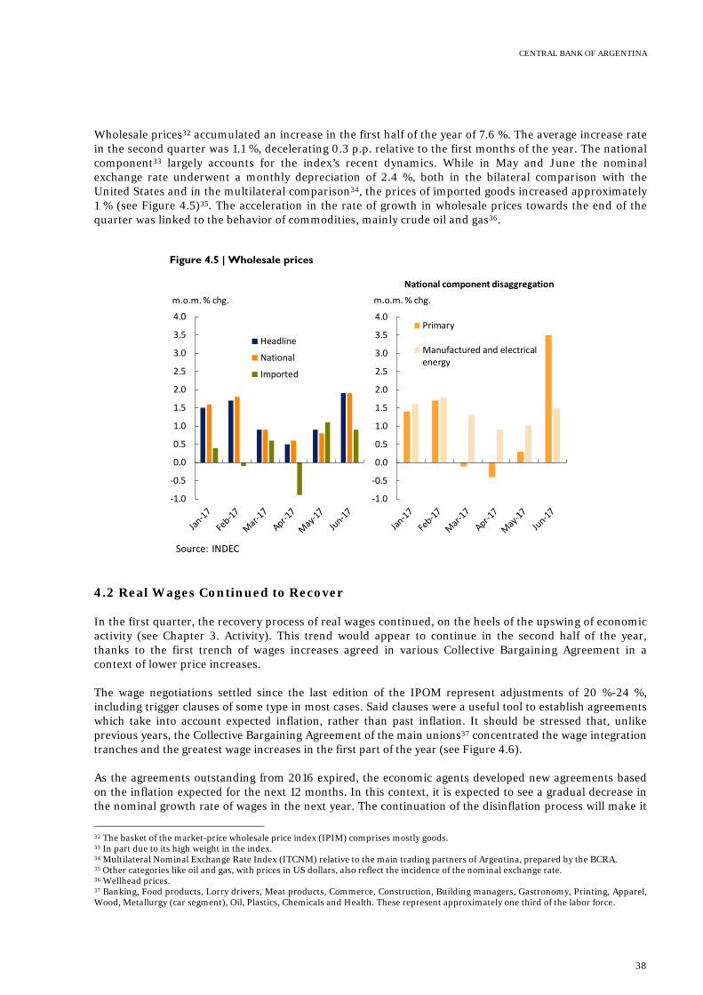
Wholesale prices32 accumulated an increase in the first half of the year of 7.6 %. The average increase rate in the second quarter was 1.1 %, decelerating 0.3 p.p. relative to the first months of the year. The national component33 largely accounts for the index’s recent dynamics. While in May and June the nominal exchange rate underwent a monthly depreciation of 2.4 %, both in the bilateral comparison with the United States and in the multilateral comparison34, the prices of imported goods increased approximately 1 % (see Figure 4.5)35. The acceleration in the rate of growth in wholesale prices towards the end of the quarter was linked to the behavior of commodities, mainly crude oil and gas36.
4.2 Real Wages Continued to Recover In the first quarter, the recovery process of real wages continued, on the heels of the upswing of economic activity (see Chapter 3. Activity). This trend would appear to continue in the second half of the year, thanks to the first trench of wages increases agreed in various Collective Bargaining Agreement in a context of lower price increases. The wage negotiations settled since the last edition of the IPOM represent adjustments of 20 %-24 %, including trigger clauses of some type in most cases. Said clauses were a useful tool to establish agreements which take into account expected inflation, rather than past inflation. It should be stressed that, unlike previous years, the Collective Bargaining Agreement of the main unions37 concentrated the wage integration tranches and the greatest wage increases in the first part of the year (see Figure 4.6). As the agreements outstanding from 2016 expired, the economic agents developed new agreements based on the inflation expected for the next 12 months. In this context, it is expected to see a gradual decrease in the nominal growth rate of wages in the next year. The continuation of the disinflation process will make it
32 The basket of the market-price wholesale price index (IPIM) comprises mostly goods. 33 In part due to its high weight in the index. 34 Multilateral Nominal Exchange Rate Index (ITCNM) relative to the main trading partners of Argentina, prepared by the BCRA. 35 Other categories like oil and gas, with prices in US dollars, also reflect the incidence of the nominal exchange rate. 36 Wellhead prices. 37 Banking, Food products, Lorry drivers, Meat products, Commerce, Construction, Building managers, Gastronomy, Printing, Apparel, Wood, Metallurgy (car segment), Oil, Plastics, Chemicals and Health. These represent approximately one third of the labor force.
Figure 4.5 | Wholesale prices
‐1.0
‐0.5
0.0
0.5
1.0
1.5
2.0
2.5
3.0
3.5
4.0
m.o.m. % chg.
Headline
National
Imported
‐1.0
‐0.5
0.0
0.5
1.0
1.5
2.0
2.5
3.0
3.5
4.0Primary
Manufactured and electricalenergy
National component disaggregation
m.o.m. % chg.
Source: INDEC
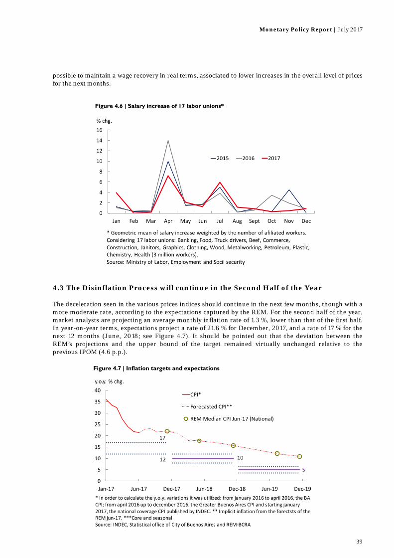
Monetary Policy Report | July 2017
39
possible to maintain a wage recovery in real terms, associated to lower increases in the overall level of prices for the next months.
4.3 The Disinflation Process will continue in the Second Half of the Year The deceleration seen in the various prices indices should continue in the next few months, though with a more moderate rate, according to the expectations captured by the REM. For the second half of the year, market analysts are projecting an average monthly inflation rate of 1.3 %, lower than that of the first half. In year-on-year terms, expectations project a rate of 21.6 % for December, 2017, and a rate of 17 % for the next 12 months (June, 2018; see Figure 4.7). It should be pointed out that the deviation between the REM’s projections and the upper bound of the target remained virtually unchanged relative to the previous IPOM (4.6 p.p.).
Figure 4.6 | Salary increase of 17 labor unions*
Figure 4.7 | Inflation targets and expectations
0
2
4
6
8
10
12
14
16
Jan Feb Mar Apr May Jun Jul Aug Sept Oct Nov Dec
% chg.
2015 2016 2017
* Geometric mean of salary increase weighted by the number of afiliated workers. Considering 17 labor unions: Banking, Food, Truck drivers, Beef, Commerce, Construction, Janitors, Graphics, Clothing, Wood, Metalworking, Petroleum, Plastic, Chemistry, Health (3 million workers).Source: Ministry of Labor, Employment and Socil security
10
5
17
12
0
5
10
15
20
25
30
35
40
Jan‐17 Jun‐17 Dec‐17 Jun‐18 Dec‐18 Jun‐19 Dec‐19
y.o.y. % chg.
CPI*
Forecasted CPI**
REM Median CPI Jun‐17 (National)
* In order to calculate the y.o.y. variations it was utilized: from january 2016 to april 2016, the BA CPI; from april 2016 up to december 2016, the Greater Buenos Aires CPI and starting january 2017, the national coverage CPI published by INDEC. ** Implicit inflation from the forectsts of the REM jun‐17. ***Core and seasonalSource: INDEC, Statistical office of City of Buenos Aires and REM‐BCRA

CENTRAL BANK OF ARGENTINA
40
In the current scenario, the main challenge will be to move core inflation back to the disinflation path in the second half. In this context, the BCRA will keep its clear anti-inflation bias, in order to ensure that the disinflation process remains on its path towards the inflation target of 12 %-17 % for 2017 and an inflation rate at end-2017 compatible with the target of 10 % ± 2 % for 2018.

Monetary Policy Report | July 2017
41
Exhibit 3 / National Consumer Price Index In July, 2017, the National Institute of Statistics and Census (INDEC) launched its nation-wide Consumer Price Index (CPI), publishing data for the January-June period of this year. On account of its being the indicator with the broadest coverage published by the INDEC, the BCRA will use it for monetary policy decisions, as was announced in September, 2016, when the inflation targeting regime was launched. The preparation of a nation-wide CPI, following homogeneous methodological definitions for the whole country, which ensure its quality and comparability at the regional level, allows us to have a trustworthy indicator of the evolution of prices, representative of the whole country. The increase in coverage, which up to this point only included the Greater Buenos Aires area (CPI-GBA), follows international recommendations, and is particularly important for the project for Argentina to enter the Organization for Economic Cooperation and Development (OECD). For its preparation, approximately 320,000 prices are compiled monthly in 40 urban conglomerates (including the city of Buenos Aires, and the 24 subdivisions which comprise the GBA), covering all provinces in the country. Price information from all the provinces, the city of Buenos Aires and the subdivisions of the GBA are grouped in 6 geographical regions: GBA, Pampeana, Argentine Northwest (NOA), Argentine Northeast (NEA), Cuyo and Patagónica. The CPI is constructed through a weighted average of regional indices, which are also disseminated. Each regional index is included in the nation-wide CPI based on the weight of urban consumption in the region relative to the total urban expenditure at the national level, based on the results of the 2004 Household Expenditure Survey 2004/05 (ENGHo 2004/05). The GBA and Pampeana regions have the greatest weight on the national indicator, with almost 80 % of the total urban households expenditure (see Figure 1).
Figure 1 | Urban household expenditure by region
GBA44.7%
Pampeana 34.2%
Northwest6.9%
Cuyo5.2%
Patagónica4.6%
Northeast4.5%
Source: INDEC

CENTRAL BANK OF ARGENTINA
42
The primary information based on which the goods and services included in each region’s CPI basket and their weight structures was selected, was also estimated based on the ENGHo 2004/05, considering consumption expenditures of resident households in urban center without exclusions of any kind. Just as in the case of the CPI-GBA, the weight structure of regional baskets was updated based on the evolution of prices between said survey’s reference period and the index base period (December, 2015), thus reflecting all eventual relative price changes seen over that period. An innovation in the publication of the nation-wide CPI and the regional CPI is the adoption of a new classification for the goods and services basket. The INDEC began disseminating the CPI results using the 1999 UN’s Classification of Individual Consumption According to Purpose (COICOP), which is an international standard. This classification comprises a first disaggregation level with 12 divisions, which are in turn divided in groups (the second disaggregation level), which are in turn divided into classes (the third level). Up to the the class level, the national classification coincides with the international one, facilitating international comparisons, as most countries use this classification, and also comparisons with the CPI of the city of Buenos Aires (see Table 1).
It is important to highlight that the use of different classifications to group data does not alter the results at the overall level, thanks to the additive property satisfied by the index’s aggregation formula38. The distribution of expenditure in 12 divisions which represent the first disaggregation level in the new classification makes it possible to describe the expenditure patterns in the different regions. Comparing the structure of the nation-wide basket with the GBA one, it can be seen that the expenditure in divisions related to services (Restaurants and hotels, Housing, Water, Power and other fuels, Health, Education, and Transportation) have a greater relative weight in the GBA than in the rest of the country. The weight of goods and services was approximately 60 % and 40 %, respectively, in the CPI-GBA as of December 2016, and in the nation-wide CPI it was of 67 % and 33 %, respectively (see Figure 2). In any event, the price changes captured by the nation-wide CPI in the first six months of 2017 are not significantly different from the CPI-GBA ones at the aggregate level. While the nation-wide CPI increased 11.8 % in the first half of 2017, the CPI-GBA increase 12.0 % over the same period.
38 Laspeyres-type formula, which in the case of the CPI is ∑ ∗∑ ∗
where n are the goods in the consumption basket with prices
and quantities, 0 is the prices’ base period (December, 2015=100), b is the reference period for the quantities stemming from the ENGHo (2004/05) and t is the current period.
Table 1 | Disaggregation levels of the CPI basket. —COICOP Classification—. Example
National COICOP Level Name Example
0 Level 0 Headline IPC. Headline
01 Level 1 Division Food and non‐alcoholic beverages
01.1 Level 2 Group Food
01.1.4 Level 3 Class Milk, milk‐based products and eggs
01.1.4.1 Level 4 Subclass Milks
01.1.4.1.001 Level 5 Variety Refrigerated whole milk
Source: INDEC
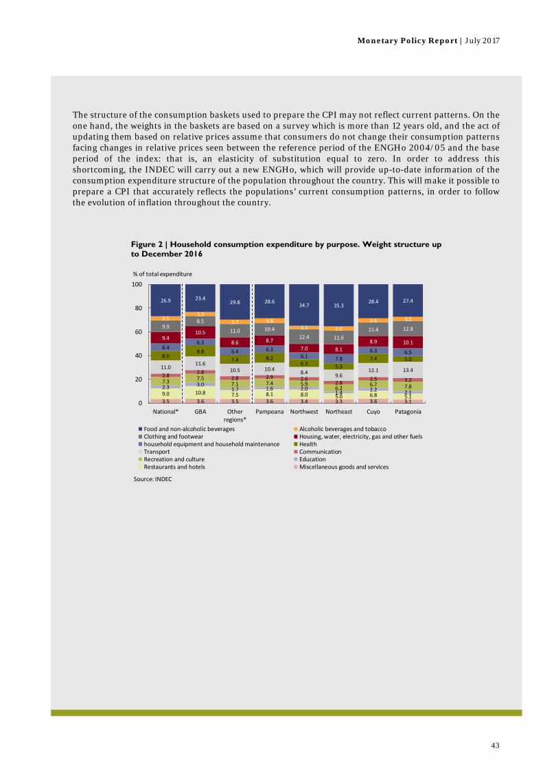
Monetary Policy Report | July 2017
43
The structure of the consumption baskets used to prepare the CPI may not reflect current patterns. On the one hand, the weights in the baskets are based on a survey which is more than 12 years old, and the act of updating them based on relative prices assume that consumers do not change their consumption patterns facing changes in relative prices seen between the reference period of the ENGHo 2004/05 and the base period of the index: that is, an elasticity of substitution equal to zero. In order to address this shortcoming, the INDEC will carry out a new ENGHo, which will provide up-to-date information of the consumption expenditure structure of the population throughout the country. This will make it possible to prepare a CPI that accurately reflects the populations’ current consumption patterns, in order to follow the evolution of inflation throughout the country.
Figure 2 | Household consumption expenditure by purpose. Weight structure up to December 2016
3.5 3.6 3.5 3.6 3.4 3.3 3.6 3.1
9.0 10.8 7.5 8.1 8.0 5.0 6.8 5.1
2.3 3.01.7 1.6 2.0
1.42.2 2.1
7.37.5
7.1 7.4 5.96.2
6.7 7.8
2.82.8
2.8 2.9 2.62.8
2.5 3.2
11.011.6
10.5 10.48.4
9.612.1 13.4
8.08.8
7.4 8.26.3
5.3
7.4 5.0
6.46.3
6.4 6.36.1 7.8
6.3 6.5
9.410.5
8.6 8.7
7.0 8.1
8.9 10.1
9.98.5
11.0 10.4
12.4 11.6
11.4 12.8
3.53.3
3.7 3.83.1 3.6
3.6 3.5
26.9 23.429.8 28.6
34.7 35.328.4 27.4
0
20
40
60
80
100
National* GBA Otherregions*
Pampeana Northwest Northeast Cuyo Patagonia
% of total expenditure
Food and non‐alcoholic beverages Alcoholic beverages and tobaccoClothing and footwear Housing, water, electricity, gas and other fuelshousehold equipment and household maintenance HealthTransport CommunicationRecreation and culture EducationRestaurants and hotels Miscellaneous goods and services
Source: INDEC

CENTRAL BANK OF ARGENTINA
44
5. Monetary Policy Starting in January, 2017, the BCRA formally adopted an inflation targeting regime, with the goal of achieving a decreasing rate of inflation over time: between 12 % and 17 % for 2017, 10 % ± 2 % for 2018, and 5 % ± 1,5 % starting in 2019. It also defined that compliance with the BCRA’s yearly targets shall be assessed based on the index with the broadest coverage published by the INDEC, which is currently the nation-wide CPI, recently developed. After nine months in which the CPI-GBA monthly core inflation fluctuated between 1.3 % and 1.9 %, and facing signs that the April inflation reading could persist in a level above the one compatible with the path defined by the monetary authority, on April 11th the BCRA established a 150 basis point increase in the policy rate, which reached 26.25 %. Even though the various monthly inflation measures resumed a decreasing path in May, as they still were above the path foreseen by the BCRA for this part of the year and as the core inflation showed signs of persistence above the level compatible with the target, the BCRA decided to keep its policy rate unchanged. Having maintained its nominal interest rate, in a context of decreasing inflation expectations, the real interest rate grew, and thus the BCRA stressed the disinflationary nature of its monetary policy. The BCRA will keep a clear anti-inflation bias in order to ensure that the disinflation process continues on its path towards a target of 12 %-17 % for 2017 and that the monthly inflation rate at end-2017 is consistent with the target of 10 % ± 2 % for 2018. 5.1 The central bank’s policy during the second quarter Starting in January, 2017, the BCRA formally adopted an inflation targeting regime, with the goal of achieving a decreasing rate of inflation over time: between 12 % and 17 % for 2017, 10 % ± 2 % for 2018, and 5 % ± 1,5 % starting in 2019. In September, 2016, it had also defined that compliance with the BCRA’s yearly targets shall be assessed based on the CPI with the broadest coverage published by the INDEC, as the monetary policy aims at reducing inflation throughout the national territory, and not in a particular region. Back then, the CPI with the greatest coverage available was the CPI-GBA, but the INDEC was progressing in the creation of a nation-wide index, which was launched in July, 2017. For the first half of the year, said indices show no significant deviations, and they are not expected to do so in the future (see Chapter 4). For that reason, the nation-wide CPI will be used to assess compliance with the BCRA’s annual target. After several months in which core inflation showed no clear signs of decreasing (see Chapter 4. Prices), and in which headline inflation moved at level higher than that compatible with the path set forth by the monetary authority, on April 11th, the BCRA increased its policy rate, the mid-band 7-days repo corridor, by 150 basis points, setting it at 26.25 %, and kept it unchanged since then. As the nominal interest rate remained unchanged, in a context of decreasing inflation expectations, the BCRA continued to stress the disinflationary nature of its monetary policy, raising the real policy rate (See Figure 5.1).

Monetary Policy Report | July 2017
45
With the goal of assessing the nature of the monetary policy, it is convenient to consider the price indices measuring core inflation. These measures provide a more accurate reading of the underlying inflation. Computing real rates taking into account core inflation expectations reduces the fluctuations created by changes in regulated and seasonal prices. Inflation expectations, as measured by the market analysts expectations survey carried out by the BCRA (REM), show a clearly decreasing trajectory for the future. Analysts expect for the BCRA to keep reducing its policy rate in the coming months, as inflation continues to decelerate, so as to keep the disinflationary nature of its policy (see Figure 5.1) However, expectations continue to deviate from the BCRA’s target for December, 2017: rather, they expect for inflation fall to 17 %, the upper bound of this year’s target, only towards the middle of 2018 (see Figure 5.2).
Figure 5.1 | Nominal and real monetary policy rate
Figure 5.2 | Inflation expectations
0
5
10
15
20
25
30
35
40
0.0
0.5
1.0
1.5
2.0
2.5
3.0
3.5
May‐16 Jul‐16 Sep‐16 Nov‐16 Jan‐17 Mar‐17 May‐17 Jul‐17 Sep‐17 Nov‐17
APR, %%
30‐day effective rate (left axis); annual nominal (right axis)
30‐day expected inflation ‐ GBA Core
30‐day real effective rate ‐ GBA Core
30‐day expected inflation ‐ National
30‐day real effective rate ‐ National
REMexpectations
Source: BCRA
35‐day LEBAC 7‐day repo corridor
12
17
10
5
21.5
14.9
9.6
0
5
10
15
20
25
30
35
40
45
50
Jun‐16
Sep‐16
Dec‐16
Mar‐17
Jun‐17
Sep‐17
Dec‐17
Mar‐18
Jun‐18
Sep‐18
Dec‐18
Mar‐19
Jun‐19
Sep‐19
Dec‐19
y.o.y. % chg.
Inflation y.o.y. (National)
REM inflation expectations 12 month (effective)
Targets
REM. Year end expectations
Source: BCRA

CENTRAL BANK OF ARGENTINA
46
So far this year, the year-on-year nation-wide inflation fell by almost 15 percentage points (p.p.), from 36.5 % in December, 2016, to 21.7 % in June, 2017, the lowest level in the last ten years. However, it continues to be 4.7 p.p. above the upper bound of the end-2017 target range. In the next few months, the BCRA will keep a clear anti-inflation bias in order to ensure that the disinflation process continues on its path towards a target of 12 %-17 % for 2017 and that the inflation rate at end-2017 is consistent with the target of 10 % ± 2 % for 2018. In order to strengthen the transmission mechanism of its policy rate to the rest of the market interest rates, the BCRA repeated its open market operations (OMA), through the sale of LEBAC in the secondary market. In this manner, it managed to remove the excess liquidity used for reverse repo with the BCRA, and managed for the LEBAC interest rate in the secondary market to recover 5 p.p. (see Figure 5.3), reaching in early July values above 26 %.
Unlike the operations carried out in 2016, when the BCRA traded in the LEBAC secondary market in the 35-day segment, in order to keep the interest rates deviation from the policy rate under half a point (which back then was the 35-day LEBAC tender), in 2017, its open market operations were distributed over all maturity tranches (see Figure 5.4).
Figure 5.3 | BCRA LEBAC secondary market operations
20
21
22
23
24
25
26
27
Feb‐28‐17 Mar‐31‐17 Apr‐30‐17 May‐31‐17 Jun‐30‐17
35‐day LEBAC LEBAC Aug‐16 LEBAC Jul‐19
LEBAC Jun‐21 LEBAC May‐17 LEBAC Apr‐19
LEBAC Mar‐15
Souce: BCRA
APR; %
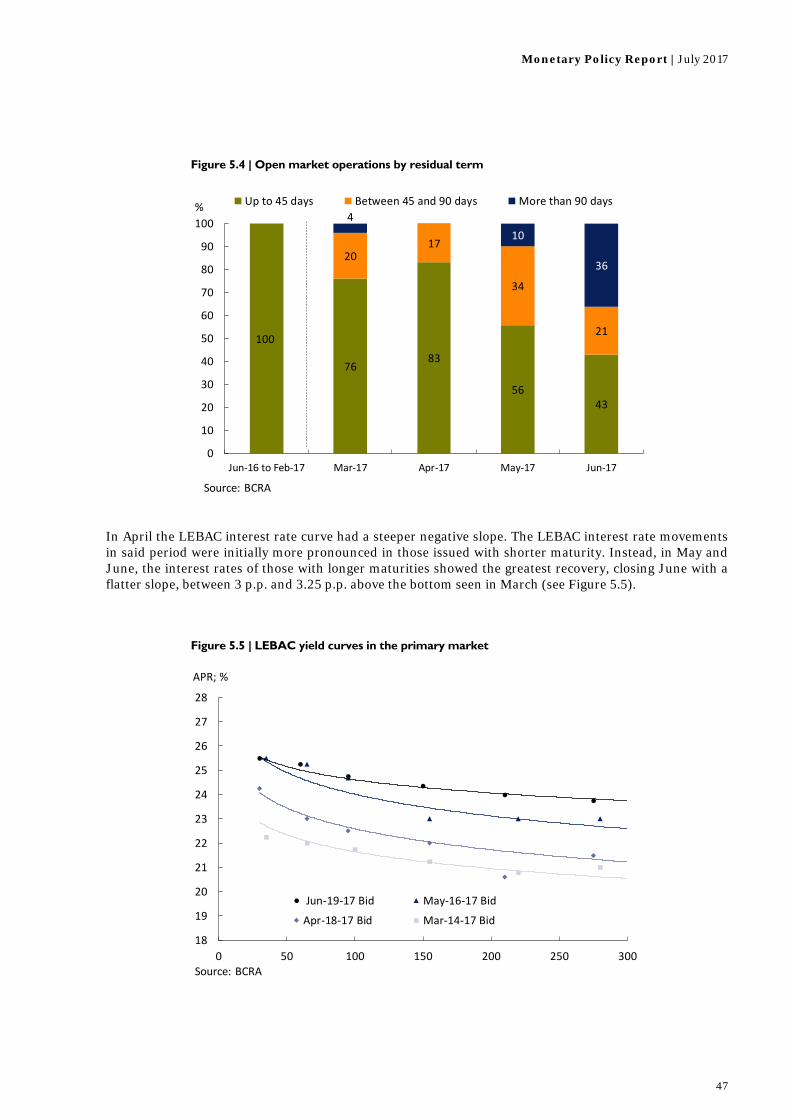
Monetary Policy Report | July 2017
47
In April the LEBAC interest rate curve had a steeper negative slope. The LEBAC interest rate movements in said period were initially more pronounced in those issued with shorter maturity. Instead, in May and June, the interest rates of those with longer maturities showed the greatest recovery, closing June with a flatter slope, between 3 p.p. and 3.25 p.p. above the bottom seen in March (see Figure 5.5).
Figure 5.4 | Open market operations by residual term
Figure 5.5 | LEBAC yield curves in the primary market
100
7683
5643
2017
34
21
4
10
36
0
10
20
30
40
50
60
70
80
90
100
Jun‐16 to Feb‐17 Mar‐17 Apr‐17 May‐17 Jun‐17
Up to 45 days Between 45 and 90 days More than 90 days%
Source: BCRA
18
19
20
21
22
23
24
25
26
27
28
0 50 100 150 200 250 300
APR; %
Jun‐19‐17 Bid May‐16‐17 Bid
Apr‐18‐17 Bid Mar‐14‐17 Bid
Source: BCRA
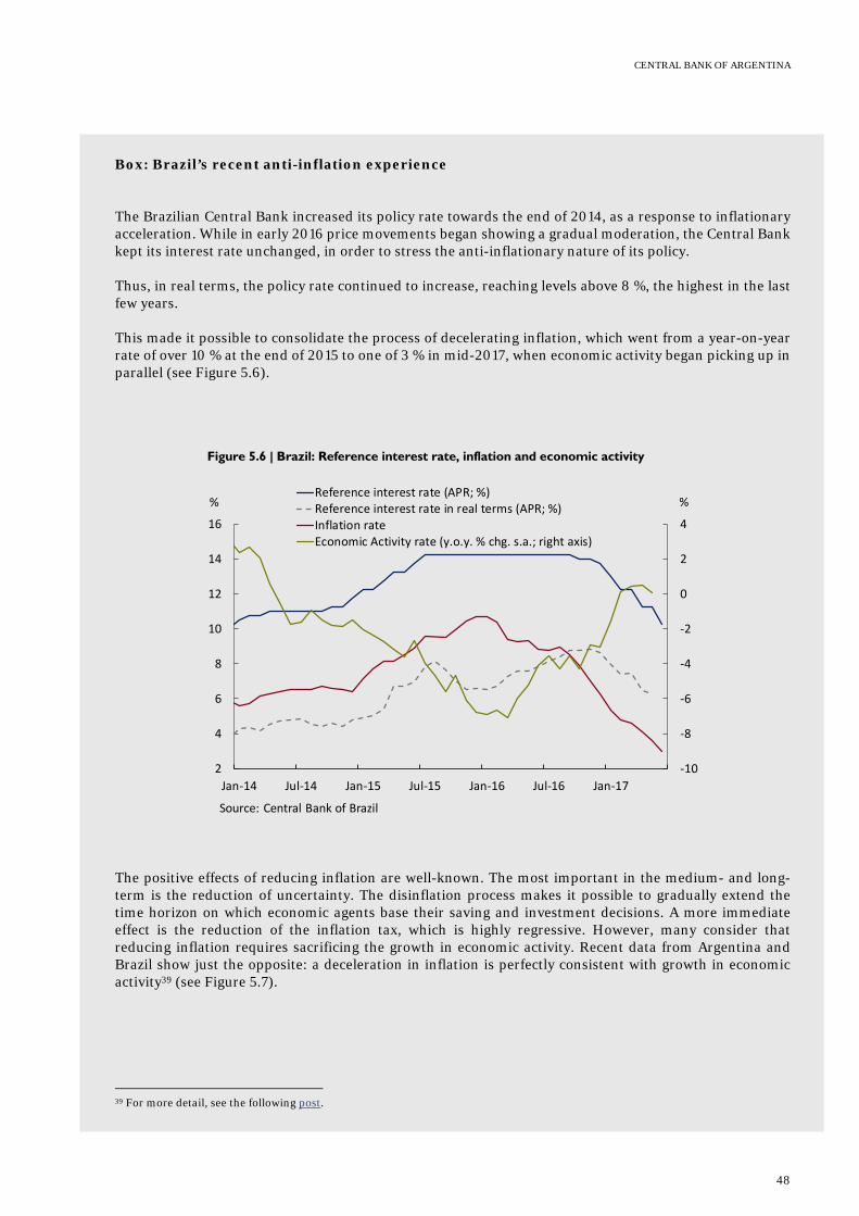
CENTRAL BANK OF ARGENTINA
48
Box: Brazil’s recent anti-inflation experience
The Brazilian Central Bank increased its policy rate towards the end of 2014, as a response to inflationary acceleration. While in early 2016 price movements began showing a gradual moderation, the Central Bank kept its interest rate unchanged, in order to stress the anti-inflationary nature of its policy. Thus, in real terms, the policy rate continued to increase, reaching levels above 8 %, the highest in the last few years. This made it possible to consolidate the process of decelerating inflation, which went from a year-on-year rate of over 10 % at the end of 2015 to one of 3 % in mid-2017, when economic activity began picking up in parallel (see Figure 5.6).
The positive effects of reducing inflation are well-known. The most important in the medium- and long-term is the reduction of uncertainty. The disinflation process makes it possible to gradually extend the time horizon on which economic agents base their saving and investment decisions. A more immediate effect is the reduction of the inflation tax, which is highly regressive. However, many consider that reducing inflation requires sacrificing the growth in economic activity. Recent data from Argentina and Brazil show just the opposite: a deceleration in inflation is perfectly consistent with growth in economic activity39 (see Figure 5.7).
39 For more detail, see the following post.
Figure 5.6 | Brazil: Reference interest rate, inflation and economic activity
‐10
‐8
‐6
‐4
‐2
0
2
4
2
4
6
8
10
12
14
16
Jan‐14 Jul‐14 Jan‐15 Jul‐15 Jan‐16 Jul‐16 Jan‐17
%%
Source: Central Bank of Brazil
Reference interest rate (APR; %)Reference interest rate in real terms (APR; %)Inflation rateEconomic Activity rate (y.o.y. % chg. s.a.; right axis)
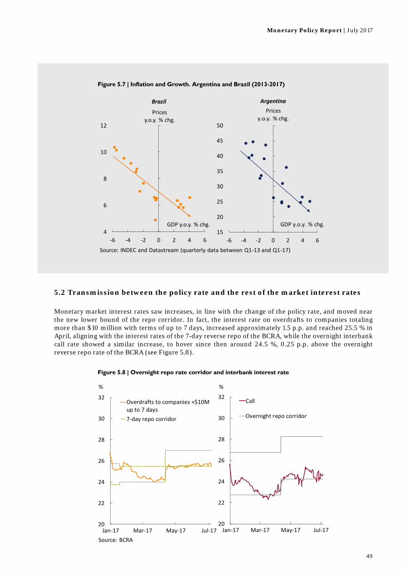
Monetary Policy Report | July 2017
49
5.2 Transmission between the policy rate and the rest of the market interest rates Monetary market interest rates saw increases, in line with the change of the policy rate, and moved near the new lower bound of the repo corridor. In fact, the interest rate on overdrafts to companies totaling more than $10 million with terms of up to 7 days, increased approximately 1.5 p.p. and reached 25.5 % in April, aligning with the interest rates of the 7-day reverse repo of the BCRA, while the overnight interbank call rate showed a similar increase, to hover since then around 24.5 %, 0.25 p.p. above the overnight reverse repo rate of the BCRA (see Figure 5.8).
Figure 5.7 | Inflation and Growth. Argentina and Brazil (2013-2017)
Figure 5.8 | Overnight repo rate corridor and interbank interest rate
4
6
8
10
12
‐6 ‐4 ‐2 0 2 4 6
Pricesy.o.y. % chg.
GDP y.o.y. % chg.15
20
25
30
35
40
45
50
‐6 ‐4 ‐2 0 2 4 6
Pricesy.o.y. % chg.
GDP y.o.y. % chg.
Source: INDEC and Datastream (quarterly data between Q1‐13 and Q1‐17)
Brazil Argentina
20
22
24
26
28
30
32
Jan‐17 Mar‐17 May‐17 Jul‐17
%
Overdrafts to companies +$10Mup to 7 days
7‐day repo corridor
Source: BCRA
20
22
24
26
28
30
32
Jan‐17 Mar‐17 May‐17 Jul‐17
%
Call
Overnight repo corridor
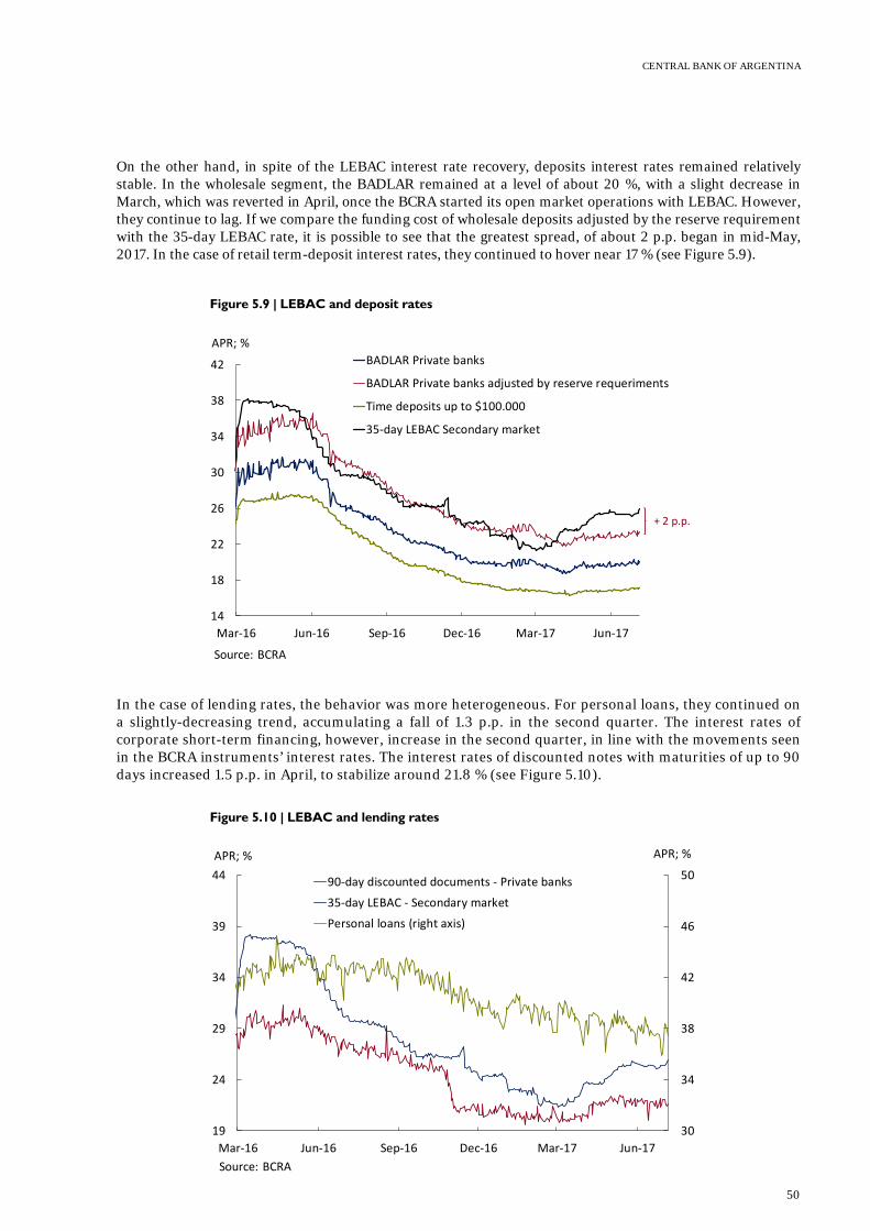
CENTRAL BANK OF ARGENTINA
50
On the other hand, in spite of the LEBAC interest rate recovery, deposits interest rates remained relatively stable. In the wholesale segment, the BADLAR remained at a level of about 20 %, with a slight decrease in March, which was reverted in April, once the BCRA started its open market operations with LEBAC. However, they continue to lag. If we compare the funding cost of wholesale deposits adjusted by the reserve requirement with the 35-day LEBAC rate, it is possible to see that the greatest spread, of about 2 p.p. began in mid-May, 2017. In the case of retail term-deposit interest rates, they continued to hover near 17 % (see Figure 5.9).
In the case of lending rates, the behavior was more heterogeneous. For personal loans, they continued on a slightly-decreasing trend, accumulating a fall of 1.3 p.p. in the second quarter. The interest rates of corporate short-term financing, however, increase in the second quarter, in line with the movements seen in the BCRA instruments’ interest rates. The interest rates of discounted notes with maturities of up to 90 days increased 1.5 p.p. in April, to stabilize around 21.8 % (see Figure 5.10).
Figure 5.9 | LEBAC and deposit rates
Figure 5.10 | LEBAC and lending rates
14
18
22
26
30
34
38
42
Mar‐16 Jun‐16 Sep‐16 Dec‐16 Mar‐17 Jun‐17
APR; %
BADLAR Private banks
BADLAR Private banks adjusted by reserve requeriments
Time deposits up to $100.000
35‐day LEBAC Secondary market
Source: BCRA
+ 2 p.p.
30
34
38
42
46
50
19
24
29
34
39
44
Mar‐16 Jun‐16 Sep‐16 Dec‐16 Mar‐17 Jun‐17
APR; %
90‐day discounted documents ‐ Private banks
35‐day LEBAC ‐ Secondary market
Personal loans (right axis)
APR; %
Source: BCRA
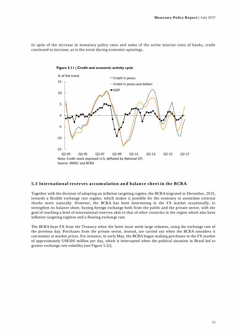
Monetary Policy Report | July 2017
51
In spite of the increase in monetary policy rates and some of the active interest rates of banks, credit continued to increase, as is the norm during economic upswings.
5.3 International reserves accumulation and balance sheet in the BCRA Together with the decision of adopting an inflation targeting regime, the BCRA migrated in December, 2015, towards a flexible exchange rate regime, which makes it possible for the economy to assimilate external shocks more naturally. However, the BCRA has been intervening in the FX market occasionally, to strengthen its balance sheet, buying foreign exchange both from the public and the private sector, with the goal of reaching a level of international reserves akin to that of other countries in the region which also have inflation targeting regimes and a floating exchange rate. The BCRA buys FX from the Treasury when the latter must settle large volumes, using the exchange rate of the previous day. Purchases from the private sector, instead, are carried out when the BCRA considers it convenient at market prices. For instance, in early May, the BCRA began making purchases in the FX market of approximately US$100 million per day, which it interrupted when the political situation in Brazil led to greater exchange rate volatility (see Figure 5.12).
Figure 5.11 | Credit and economic activity cycle
‐15
‐10
‐5
0
5
10
15
Q2‐03 Q2‐05 Q2‐07 Q2‐09 Q2‐11 Q2‐13 Q2‐15 Q2‐17
% of the trendCredit in pesos
Credit in pesos and dollars
GDP
Nota: Credit stock expresed in $, deflated by National CPI. Source: INDEC and BCRA

CENTRAL BANK OF ARGENTINA
52
All in all, US$3.1 billion were purchased during the second quarter, and an additional US$500 million in the first half of July (see Figure 5.13).
Figure 5.12 | Exchange rate and purchases and sales on the exchange market
Figure 5.13 | BCRA purchases on the exchange markets
8.5
10.5
12.5
14.5
16.5
18.5
‐800
0
800
1,600
2,400
3,200
Jan‐15 May‐15 Sep‐15 Jan‐16 May‐16 Sep‐16 Jan‐17 May‐17
$/US$Net purchases to the National Treasury
Net purchases to the rest of counterparties
Reference exchange rate (right axis)
Elimination of clamp
Brexit
U.S elections
Source: BCRA
Brazil politic
situation
million US$
2,000
1,100
0
500
‐1,000
‐500
0
500
1,000
1,500
2,000
2,500
3,000
3,500
Jan‐16 Mar‐16 May‐16 Jul‐16 Sep‐16 Nov‐16 Jan‐17 Mar‐17 May‐17 Jul‐17
million US$
*Data up to July 14. Source: BCRA
*

Monetary Policy Report | July 2017
53
Exhibit 4 / An alternative look at the BCRA balance sheet The analysis of an entity’s equity can be approached according to different criteria, depending on the aspect to be studied. It is possible to focus, for instance, on its creditworthiness level, or the liquidity of its different assets, both in terms of present or face value and of what could be expected in the future, among many other variables. Along that line, this exhibit presents a study about the BCRA’s equity based on an approach which differs from one based exclusively on accounting. Figure 1 shows the BCRA’s net worth, expressed in US dollars40, based on two alternative criteria. The red line shows the institution’s net worth as is reflected in its balance sheet every year since 2003. As shown, it has always remained in positive values during the period at hand.
However, not all assets included in the balance sheet have the same level of liquidity. Particularly, it includes Non-Transferable Bills (securities extended by the Treasury as a counterpart for the use of international reserves) and Temporary Advances (the stock of peso-denominated loans the BCRA can extend to the Treasury as provided in Article 20 of its Charter41). A particular aspect shared by both assets is that neither can be traded in the markets, and so their degree of liquidity is very small in comparative terms. It is thus relevant to assess how the entity’s net worth evolved discounting the value of these nontradable assets. In Figure 1, blue bars show this alternate concept. The figure shows that the path over time of both measures differs radically. According to the second approach, the entity’s net worth turned negative in 2006 (when approximately US$9.5 billion of international reserves were used to repay a debt with the International Monetary Fund). Afterwards, it remained relatively stable until 2010, when its dynamics undergoes a qualitative change and begins deteriorating quickly. Between end-2009 and the last public administration change at the national level, it decreased the equivalent of US$ 86.86 billion dollars. This phenomenon is mainly accounted for by the
40 According to the benchmark peso-dollar exchange rate of each day, published in Communication “A” 3500. 41 Law No. 24144 and amendments.
Figure 1 | BCRA net worth based on two alternative criteria
782 1,217 1,594‐7,960‐6,984‐8,545‐6,111
‐18,000
‐32,642
‐47,000
‐54,465
‐70,552
‐92,971
‐60,268‐64,330
3,293 5,692 6,872 7,727 9,522 8,80213,084
9,714 8,68312,470
16,45712,698
5,084
13,6378,493
‐100,000
‐90,000
‐80,000
‐70,000
‐60,000
‐50,000
‐40,000
‐30,000
‐20,000
‐10,000
0
10,000
20,000
30,000
million US$
Net worth discounting illiquid assets
Net worth (balance sheet)
CENTRAL BANK OF ARGENTINA
54
issuance of Non-Transferable Bills for a value of approximately US$ 55 billion, and an increase of US$23.9 billion in Temporary Advances42. That is, the interpretation of the BCRA’s balance sheet varies significantly if the government securities and illiquid loans taken as part of its assets are considered separately43. However, we should note that it would not be technically correct to discount the whole amount represented by the aforementioned securities, as it is possible to swap them for more liquid assets, as was done in late 2015, with the Treasury Non-Transferable Bills (the 2006 issuance and two 2010 issuances), for a total of US$16 billion, swapped for new issuances of BONAR 2022, BONAR 2025 and BONAR 2027, all of which are tradable in financial markets. Moreover, an additional aspect which is often overlooked when analyzing the central bank’s balance sheet is the importance of seigniorage as a source of income for the monetary authority. This refers to the real resources the bank collects for issuing money the public wants to keep. It is based on the fact that the BCRA issues a liability which pays no interest (and with a small marginal issuance cost), but is demanded for economic agents to be used as a means of payment and store of value. This income can be broken down into two factors: 1) the public’s intention to modify its money demand (its real balances), which depends on the interest rate and the level of economic activity; and 2) the inflation tax, that is, the loss of purchasing power associated with holding money, due to the effect of inflation, which represents a resource transfer from the public to the government. In this context, it is possible to run a simple exercise to compute the present value of seigniorage, in order to assess its relevance in the BCRA accounts from a more “economic” standpoint, not as focused on accounting. Considering a scenario in which the economy grows 3 % per year (close to the average expansion of the Argentine economy in the last 100 years), with an annual inflation rate of 5 %, and with a stable high-powered money of 10 % of GDP (near the current level), we arrive at an annual seigniorage of 0.8 % of GDP. This flow can be broken down into a 0.3 % of GDP linked to the growth in the money demand, due to the expansion of the economy, and a 0.5 % of GDP linked to the inflation tax44. If this income flow is considered as if it was a perpetuity and is discounted with a real annual interest rate of 4 %, the present value of seigniorage stands at 79 % of GDP45. It can be seen, then, that this source of resources reaches a significant magnitude relative to the nonmonetary liabilities held by the BCRA, and proves the need of taking them into account when analyzing the inter-temporal sustainability of its accounts comprehensively. In sum, once these elements have been considered, it is possible to posit two complementary ways of approaching the analysis of the BCRA balance sheet: one purely focused on accounting aspects (based directly on the published balance sheet), and a second, more “economic” in nature, based on what was detailed above. Now we present the simplified results showing what the BCRA balance sheet would look like based on each approach: 42 It is worth remembering that the reform of the BCRA Charter established in March, 2012, expanded the ceiling for the issuance of Temporary Advances to the Treasury. 43 In this line, it should be mentioned that the BCRA will implement the International Financial Reporting Standards (IFRS) for the preparation of its balance sheet starting in 2018. Based on that change in methodology, its portfolio securities will now be valued at market prices. 44 While the inflationary tax is not desirable in distributional terms, the inflation rate used in the exercise is at the levels seen in the region’s economies and other emerging economies, and is the result of achieving price stability. Besides, this inflation rate provides the monetary policy with room to avoid the issue of the zero lower bound for the nominal interest rate (which is not currently a problem of Argentina, but could turn problematic in the future, after the disinflation process). 45 The present value of seigniorage with the variables in long term values can be expressed as follows:
∆ 1
Where ∆
is the annual seigniorage in terms of GDP (0.8 % of GDP for all periods), is the real interest rate (4 %), and
is the growth rate of the economy (3 %). The present value of seigniorage can also be expressed considering the present value of the interest not paid for using a monetary liability, less the initial high-powered money stock:
This is the way in which seigniorage is expressed in the economic balance of Table 1. For a detailed analysis of the computation of seigniorage by the government, see Buiter, W. (2007): “Seigniorage”, NBER, working document No. 12919.

Monetary Policy Report | July 2017
55
The left-hand table is simply a summary version of the institution’s accounting balance sheet, while the right-hand one shows the present value of net seigniorage and discounts from the asset the amount of nontradable assets (temporary advances and nontransferable bills). The present value of net seigniorage is computed based on the assumptions detailed above, with a real annual interest rate of 4 %, deducting the BCRA’s expenditures (at their current level as a percentage of GDP), and the monetary assistance to the government (which converges towards zero), and assuming the uncovered interest rates parity is respected at all times. As can be seen, even though deducting illiquid assets implies a marked downward revision of the net worth, from the point of view of creditworthiness, the BCRA has resources which more than offset this deterioration, which is why the net worth in the right-hand table is markedly higher. Even if some of the exercise’s assumptions are modified to create scenarios with a lower level of annual seigniorage, as a reduction in the high-powered money-GDP ratio to 7 %, for instance, due to an increase in the use of electronic means of payment (greater use of transactional deposits and lower use of notes and coins), or a fall in long-term annual inflation to 3 %, the “economic” net worth remains in high levels (falling from 65.5 % of GDP to 37.5 % and 46.7 %, respectively).
Table 1 | BCRA balance sheet from “countable” and “acounting” approach (% of GDP, up to Dec. 31, 2016)
International reserves 7.6% monetary base 10.2% International reserves 7.6% Monetary base 10.2%
Non‐Transferable Bills 9.6% Liabilities in US$ 5.3% Non‐Transferable Bills 0.0% Liabilities in US$ 5.3%
Government securities in US$ 3.4% LEBAC and Net repos 8.8% Government securities in US$ 3.4% LEBAC and Net repos 8.8%
Government securities in $ 0.6% Government securities in $ 0.6%
Temporary Advances and other
net assets in $4.7%
Temporary Advances and
other net assets in $0.0%
Net seigniorage 78.2%
Net worth 1.7% Net worth 65.5%
"Accounting" "Economic"
Asset Liability and Net worth Asset Pasivo y PN
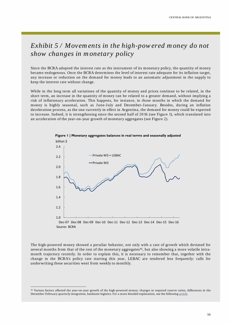
CENTRAL BANK OF ARGENTINA
56
Exhibit 5 / Movements in the high-powered money do not show changes in monetary policy Since the BCRA adopted the interest rate as the instrument of its monetary policy, the quantity of money became endogenous. Once the BCRA determines the level of interest rate adequate for its inflation target, any increase or reduction on the demand for money leads to an automatic adjustment in the supply to keep the interest rate without change. While in the long term all variations of the quantity of money and prices continue to be related, in the short term, an increase in the quantity of money can be related to a greater demand, without implying a risk of inflationary acceleration. This happens, for instance, in those months in which the demand for money is highly seasonal, such as June-July and December-January. Besides, during an inflation deceleration process, as the one currently in effect in Argentina, the demand for money could be expected to increase. Indeed, it is strengthening since the second half of 2016 (see Figure 1), which translated into an acceleration of the year-on-year growth of monetary aggregates (see Figure 2).
The high-powered money showed a peculiar behavior, not only with a rate of growth which deviated for several months from that of the rest of the monetary aggregates46, but also showing a more volatile intra-month trajectory recently. In order to explain this, it is necessary to remember that, together with the change in the BCRA’s policy rate starting this year, LEBAC are tendered less frequently: calls for underwriting these securities went from weekly to monthly. 46 Various factors affected the year-on-year growth of the high-powered money: changes in required reserve ratios, differences in the December-February quarterly integration, banknote logistics. For a more detailed explanation, see the following article.
Figure 1 | Monetary aggregates balances in real terms and seasonally adjusted
1.0
1.2
1.4
1.6
1.8
2.0
2.2
2.4
Dec‐07 Dec‐08 Dec‐09 Dec‐10 Dec‐11 Dec‐12 Dec‐13 Dec‐14 Dec‐15 Dec‐16
billion $
Private M3 + LEBAC
Private M3
Source: BCRA

Monetary Policy Report | July 2017
57
Given the flexibility of reserve requirements, which must be complied with taking into account monthly average balances, the concentration of LEBAC maturities on the third Wednesday of each month, and the strategy used by banks to manage their liquidity, translated into temporary expansions of the high-powered money on the LEBAC due dates, which were reverted in the remaining days of the month (see Figure 3). Particularly, the financial entities partially rolled-over the LEBAC maturities, creating an excess in their reserve requirement positions, offset during the rest of the month.
Figure 2 | Monetary aggregates variation
Figure 3 | monetary base balance
15
20
25
30
35
40
45
50
Jun‐12 Jun‐13 Jun‐14 Jun‐15 Jun‐16 Jun‐17
y.o.y. % chg.
Monetary Base
Private M2
Private M3
M3
Source: BCRA
750
770
790
810
830
850
870
890
Mar‐1‐17 Apr‐1‐17 May‐1‐17 Jun‐1‐17
billion $
National Treasury bond
Money demand seasonality
LEBACmaturities

CENTRAL BANK OF ARGENTINA
58
Additionally, in June, the Treasury placed a peso-denominated bond with a 2020 maturity for a total of $75 billion (nominal value), settled on the third Wednesday in June, the LEBAC due date. 70 percent of this security was underwritten in pesos, with most of the funds used for the underwriting coming from LEBAC. For this reason, during June’s LEBAC tender, there was a monetary expansion much greater than that of the previous months, which heightened the aforementioned behavior. Another factor which also affected that tender’s result was the seasonal increase in the demand of liquidity of late June and early July, related to the 13th month salary and the winter vacations.
In sum, all these factors provide the high-powered money with a behavior which should not be mistaken with a change in the monetary policy’s nature. If the BCRA keeps its policy rate unchanged, potential increases or reductions in the high-powered money do not mean that the BCRA has adopted a more expansionary or restrictive policy.
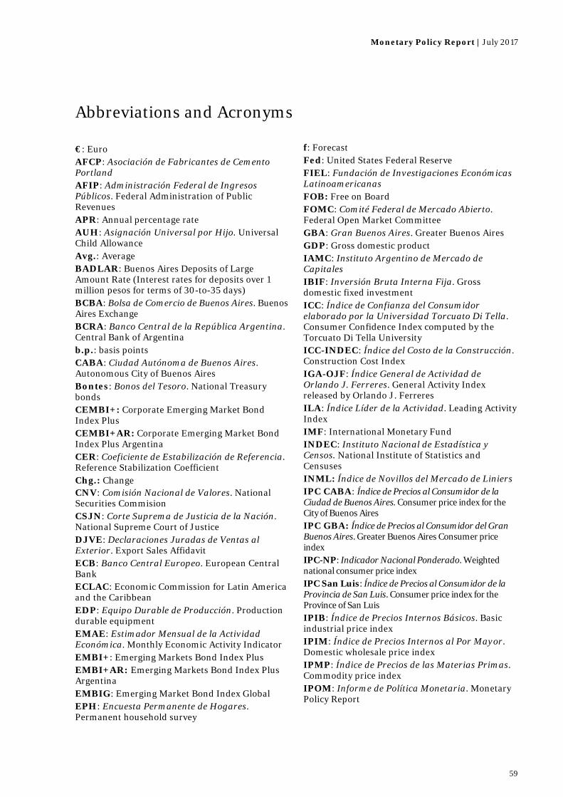
Monetary Policy Report | July 2017
59
Abbreviations and Acronyms €: Euro AFCP: Asociación de Fabricantes de Cemento Portland AFIP: Administración Federal de Ingresos Públicos. Federal Administration of Public Revenues APR: Annual percentage rate AUH: Asignación Universal por Hijo. Universal Child Allowance Avg.: Average BADLAR: Buenos Aires Deposits of Large Amount Rate (Interest rates for deposits over 1 million pesos for terms of 30-to-35 days) BCBA: Bolsa de Comercio de Buenos Aires. Buenos Aires Exchange BCRA: Banco Central de la República Argentina. Central Bank of Argentina b.p.: basis points CABA: Ciudad Autónoma de Buenos Aires. Autonomous City of Buenos Aires Bontes: Bonos del Tesoro. National Treasury bonds CEMBI+: Corporate Emerging Market Bond Index Plus CEMBI+AR: Corporate Emerging Market Bond Index Plus Argentina CER: Coeficiente de Estabilización de Referencia. Reference Stabilization Coefficient Chg.: Change CNV: Comisión Nacional de Valores. National Securities Commision CSJN: Corte Suprema de Justicia de la Nación. National Supreme Court of Justice DJVE: Declaraciones Juradas de Ventas al Exterior. Export Sales Affidavit ECB: Banco Central Europeo. European Central Bank ECLAC: Economic Commission for Latin America and the Caribbean EDP: Equipo Durable de Producción. Production durable equipment EMAE: Estimador Mensual de la Actividad Económica. Monthly Economic Activity Indicator EMBI+: Emerging Markets Bond Index Plus EMBI+AR: Emerging Markets Bond Index Plus Argentina EMBIG: Emerging Market Bond Index Global EPH: Encuesta Permanente de Hogares. Permanent household survey
f: Forecast Fed: United States Federal Reserve FIEL: Fundación de Investigaciones Económicas Latinoamericanas FOB: Free on Board FOMC: Comité Federal de Mercado Abierto. Federal Open Market Committee GBA: Gran Buenos Aires. Greater Buenos Aires GDP: Gross domestic product IAMC: Instituto Argentino de Mercado de Capitales IBIF: Inversión Bruta Interna Fija. Gross domestic fixed investment ICC: Índice de Confianza del Consumidor elaborado por la Universidad Torcuato Di Tella. Consumer Confidence Index computed by the Torcuato Di Tella University ICC-INDEC: Índice del Costo de la Construcción. Construction Cost Index IGA-OJF: Índice General de Actividad de Orlando J. Ferreres. General Activity Index released by Orlando J. Ferreres ILA: Índice Líder de la Actividad. Leading Activity Index IMF: International Monetary Fund INDEC: Instituto Nacional de Estadística y Censos. National Institute of Statistics and Censuses INML: Índice de Novillos del Mercado de Liniers IPC CABA: Índice de Precios al Consumidor de la Ciudad de Buenos Aires. Consumer price index for the City of Buenos Aires IPC GBA: Índice de Precios al Consumidor del Gran Buenos Aires. Greater Buenos Aires Consumer price index IPC-NP: Indicador Nacional Ponderado. Weighted national consumer price index IPC San Luis: Índice de Precios al Consumidor de la Provincia de San Luis. Consumer price index for the Province of San Luis IPIB: Índice de Precios Internos Básicos. Basic industrial price index IPIM: Índice de Precios Internos al Por Mayor. Domestic wholesale price index IPMP: Índice de Precios de las Materias Primas. Commodity price index IPOM: Informe de Política Monetaria. Monetary Policy Report
CENTRAL BANK OF ARGENTINA
60
ITCRM: Índice de Tipo de Cambio Real Multilateral. Real Multilateral Exchange Rate Index LAC: Latin American Consensus Forecasts LEBAC: Letras del Banco Central. BCRA bills LFPIF: Línea de financiamiento para la producción y la inclusión financiera M2: Billetes y monedas + cuasimonedas en circulación + cuentas corrientes en $ y cajas de ahorro en $. Notes and coins + quasimonies + $ savings and current accounts m.a.: moving average MATBA: Mercado a Término de Buenos Aires MERVAL: Mercado de Valores de Buenos Aires MIP: Matriz insumo-producto. Input-output matrix MOA: Manufacturas de Origen Agropecuario. Manufactures of agricultural origin MOI: Manufacturas de Origen Industrial. Manufactures of industrial origin MSCI: Morgan Stanley Capital International Index MTEySS: Ministerio de Trabajo, Empleo y Seguridad Social. Ministry of Labor, Employment and Social Security MULC: Mercado Único y Libre de Cambios. Single free exchange market National IPC: Índice de Precios al Consumidor Nacional. National consumer price index NOBAC: Notas del Banco Central. BCRA notes OPEC: Organization of the Petroleum Exporting Countries p.p.: Percentage points PCP-BCRA: Predicción contemporánea del BCRA
PMI: Purchasing Managers’ Index PP: Productos primaries. Primary products R$: Brazilian Real REM: Relevamiento de Expectativas de Mercado. Market Expectations Survey REPO: Repurchase Agreement ROE: Registros de Operaciones de Exportación. Export operations records Rueda REPO: Tasa de interés promedio de las operaciones a 1 día hábil entre entidades financieras en el mercado garantizado s.a.: Seasonally adjusted TFP: Productividad total de los factores. Total factor productivity TN: Tesoro Nacional. National Treasury UCI: Utilización de la capacidad instalada. Installed capacity utilization US$: United States Dollar UTA: Unión Tranviarios Automotores UTDT: Universidad Torcuato Di Tella. Torcuato Di Tella University UVA: Unidad de Valor Adquisitivo. Acquisition Value Unit VAR: Modelo de Vectores Autorregresivos. Vector Autorregresive Models VAT: Value added tax VBP: valor bruto de producción. Gross production value y.o.y.: year-on-year YPF SA: Yacimientos Petrolíferos Fiscales Sociedad Anónima