Monetary policy regimes and capital account restrictions in a small

FEDERAL RESERVE BANK OF SAN FRANCISCO

WORKING PAPER SERIES

Optimal Monetary Poilicy and Capital Account

Restrictions in a Small Open Economy

Zheng Liu Federal Reserve Bank of San Francisco

Mark M. Spiegel

Federal Reserve Bank of San Francisco

February 2015

The views in this paper are solely the responsibility of the authors and should not be interpreted as reflecting the views of the Federal Reserve Bank of San Francisco or the Board of Governors of the Federal Reserve System.

Working Paper 2013-33 http://www.frbsf.org/publications/economics/papers/2013/wp2013-33.pdf

http://www.frbsf.org/publications/economics/papers/2013/wp2013-33.pdf

OPTIMAL MONETARY POLICY AND CAPITAL ACCOUNTRESTRICTIONS IN A SMALL OPEN ECONOMY

ZHENG LIU AND MARK M. SPIEGEL

Abstract. Declines in interest rates in advanced economies during the global fi-nancial crisis resulted in surges in capital flows to emerging market economies andtriggered advocacy of capital control policies. We evaluate the effectiveness formacroeconomic stabilization and the welfare implications of the use of capital ac-count policies in a monetary DSGE model of a small open economy. Our modelfeatures incomplete markets, imperfect asset substitutability, and nominal rigidi-ties. In this environment, policymakers can respond to fluctuations in capital flowsthrough capital account policies such as sterilized interventions and taxing capitalinflows, in addition to conventional monetary policy. Our welfare analysis suggeststhat optimal sterilization and capital controls are complementary policies.

Date: February 23, 2015.Key words and phrases. capital controls, sterilization, optimal policy, capital flows, open-economy.JEL classification: F31, F32, E42.

Liu: Federal Reserve Bank of San Francisco, 101 Market Street, San Francisco, CA 94105(email: [email protected]). Spiegel: Federal Reserve Bank of San Francisco, 101 MarketStreet, San Francisco, CA 94105 (email: [email protected]). We thank Olivier Blanchard,Pierre-Olivier Gourinchas, Young Sik Kim, seminar participants at the Federal Reserve Bank of SanFrancisco, the IMF-BOK conference on “Asia: Challenges of Stability and Growth,” the Banque deFrance, the 7th Annual MIFN Conference, UC Santa Cruz, and an anonymous referee for helpfulcomments. The views expressed herein are those of the authors and do not necessarily reflect theviews of the Federal Reserve Bank of San Francisco or the Federal Reserve System.

1

OPTIMAL MONETARY POLICY AND CAPITAL CONTROLS 2

I. Introduction

In the wake of the recent global financial crisis, central banks in advanced economiesreduced global interest rates dramatically. Small open economies that were perceivedas having desirable growth prospects experienced surges of foreign capital inflows[e.g. Ghosh et al. (2014)]. Many commentators argue that these capital inflowsassociated with easy monetary policies in advanced economies posed potential threatsto emerging market economies by pushing up inflation. Moreover, sudden reversalsin capital flows could pose challenges for financial stability in the capital recipientcountries.1

Concerns about the potential risks posed by surges in capital flows have led toreconsideration of the merits of capital control policies (Ostry et al., 2010). Conven-tional monetary policy is likely to be ineffective in mitigating surges in capital inflowsin small open economies, as raising interest rates can have the counterproductive effectof raising the attractiveness of a nation as a destination for foreign investment [e.g.Rey (2013)]. Still, if assets are imperfect substitutes, sterilization may be effectivelyused as a policy response. By using a combination of capital account restrictions andsterilization of capital flows, a central bank can mitigate the effects of excess foreigncapital flows caused by external shocks [e.g. Fernandez-Arias and Montiel (1996),Farhi and Werning (2012) and Unsal (2013)].

However, capital controls and sterilization policies can be costly. Capital controlscan be distortionary [e.g. Edwards (1999), Johnson and Mitton (2003)]. Similarly,sterilization policies can have adverse fiscal implications in environments with lowprevailing global interest rates. These costs must be incorporated in the pursuitof optimal policy. For example, Chang et al. (2012) show that the large increasesin the spread between domestic and foreign interest rates following the crisis raisedsubstantially the cost of sterilization for the People’s Bank of China (PBOC).2 Inthe wake of an unexpected decline in foreign interest rates, optimal monetary policyin such an environment includes slowing the pace of sterilization and allowing forincreased inflation.

In this paper, we study the effectiveness of capital controls and sterilization policiesin a small open economy with incomplete markets and imperfect asset substitutability.

1Central bankers in advanced economies defended these policies by maintaining that they wereappropriate for stimulating their domestic economies, and that ensuring the recovery of the advancedeconomies was also in the interest of the emerging economies [e.g. Bernanke (2012)].

2The PBOC engages in extensive sterilization activity to maintain the country’s closed capitalaccount in the face of persistent Chinese current account surpluses.


Our model generalizes the standard small open economy model of Schmitt-Grohé andUribe (2003) in three dimensions. First, to study the macroeconomic and welfareimplications of sterilization policies, we introduce imperfect substitutability betweendomestic and foreign assets. Specifically, we incorporate adjustment costs for privateholdings of foreign and domestic assets. These costs drive a wedge into the standarduncovered interest rate parity (UIP) condition and result in imperfect risk sharingacross countries. Second, to study optimal capital control policies, we introduce atime-varying tax on capital inflows. Third, to allow monetary policy to have realeffects, we assume that prices are sticky.

We consider optimal Ramsey policy under which the Ramsey planner maximizesthe representative household’s welfare, taking private sector optimizing decisions asgiven. In our benchmark model, the planner makes use of not just the conventionalmonetary policy instruments, but also sterilization activity and capital control policiesto maximize welfare.3 Sterilization activity takes the form of optimally adjusting thecentral bank’s foreign bond portfolio, while capital control policies are modeled aslevying an optimal time-varying tax on foreign earnings on domestic bonds.4

Imperfect asset substitutability in the model inhibits international risk sharing andraises the scope for capital account policies to influence macroeconomic stability andwelfare. Thus, unlike the standard small open economy model such as that in Galíand Monacelli (2005), even if there are no markup shocks and fiscal subsidies areavailable to offset steady-state markup distortions, monetary policy in general cannotcompletely stabilize the welfare-relevant output gap (Corsetti et al., forthcoming).However, this same imperfect asset substitutability allows the central bank to engagein sterilization activity to insulate the economy from external shocks and surges incapital inflows. We therefore explicitly model the central bank’s balance-sheet deci-sions to illustrate the macroeconomic effects of sterilization activity. In addition, weconsider the implications of direct capital controls in the form of optimal taxation offoreign earnings on domestic bonds.

Importantly, acting alone, neither of these capital account policies are capable offully addressing the frictions associated with imperfect asset substitution. Sterilizationcan influence asset demands, but has fiscal implications that impact on the governmentbudget constraint. Taxes on capital inflows influence foreign demand for domestic

3The Ramsey policy problem that we consider here is similar to the jointly optimal fiscal andmonetary policy problem studied by Schmitt-Grohé and Uribe (2004).

4Time-varying capital flow restrictions have been considered in a different context in previousstudies [e.g., Jeanne and Korinek (2010) and Korinek (2013)].


assets, but do not directly address the impact of external shocks on domestic householdasset demands. Moreover, taxing foreign returns on domestic assets introduces awedge between domestic and foreign returns, raising distortions.5 As such, the jointimplementation of both optimal sterilization and capital control policies has potentialfor improving social welfare, even relative to optimal use of the other stabilizing policyin isolation.

We calibrate our model to examine the effectiveness of the two types of capitalaccount polices – sterilization and capital controls – for macroeconomic stability. Wealso evaluate welfare outcomes under alternative policy regimes where the Ramseyplanner cannot optimally set one or both of the capital account policies.

Our benchmark results suggest that optimal policy makes use of both sterilizationand capital controls in the presence of external interest rate shocks or domestic tech-nology shocks. For example, in the wake of a negative foreign interest rate shock in ourmodel, the planner raises simultaneously the government’s holdings of foreign reservesand the tax rate on capital inflows. In our calibrated results below, the combination ofthese polices succeeds in smoothing macroeconomic volatility and increasing welfare.

We then consider three alternative regimes to isolate the impacts of the capitaltax and sterilization policies. We first shut off each of these policies in isolationsequentially, and then shut off both of them at once. We shut off sterilization activityby forcing the government foreign reserve holdings to be constant at the steady statelevel over the course of the business cycle; similarly, when we shut off the capitalcontrol policies, we restrict the capital inflow tax to its steady state value throughoutthe cycle. Comparisons of the welfare outcomes across these regimes, along withour benchmark results, demonstrate the marginal welfare enhancement of introducingeach of the policies.

Our welfare results indicate that introducing optimal capital controls policy in anenvironment with optimal sterilization results in much larger gains than doing soin an environment where the central bank does not sterilize. These results thereforesuggest that capital controls and sterilization policies are complementary in addressingexternal shocks, rather than substitutes. The sensitivity of our conclusions concerningthe efficacy of capital controls policies in stabilizing the economy also demonstrates

5A more comprehensive set of capital controls, with different tax schedules to accommodate dif-ferences in domestic and foreign asset demand, may mitigate the welfare gains from also engagingin sterilization. However, such a policy would likely be difficult to implement, as it would requiredifferent schedules for all of the adjustment margins considered.


the importance of accurate portrayal of the overall policy toolkit when evaluatingindividual stabilization policies.

The remainder of this paper is divided into four sections. Section II discusses thecontributions of this paper relative to literature. Section III introduces the benchmarkDSGE model that features imperfect asset substitutability and nominal rigidities.Section IV presents the optimal policy problem and discusses the effectiveness ofsterilization and capital control policies for macroeconomic stabilization. There, wealso study the welfare implications of alternative policy regimes. Finally, Section Vprovides some concluding remarks. Some detailed derivations of Ramsey optimalpolicy problem are presented in the Appendix.

II. Related Literature

The DSGE model that we examine here provides a coherent theoretical frameworkfor studying optimal monetary policy and for evaluating welfare performances of al-ternative policy regimes. In the standard DSGE model of a closed economy, monetarypolicy faces no trade off between stabilizing inflation and stabilizing the output gap(Blanchard and Galí, 2007). This “divine coincidence,” which is obtained from a closedeconomy model, can be carried over to a small open economy with perfect interna-tional capital flows and flexible exchange rates (Clarida et al., 2002). Indeed, Obstfeldand Rogoff (2002) show that the gains from international policy coordination may belimited relative to welfare attainable from “self-oriented” monetary policies gearedtowards national macroeconomic goals. Subsequent literature shows that the divinecoincidence breaks down in more general environments, such as one with multiplesources of nominal rigidities. Examples include a model with sticky prices and stickynominal wages (Erceg et al., 2000), a model with sticky prices in multiple sectors(Mankiw and Reis, 2003; Huang and Liu, 2005), and a model with multiple countries(Benigno, 2004; Liu and Pappa, 2008; Monacelli, 2013). For a survey of the litera-ture on optimal monetary policy in open economies, see, for example, Corsetti et al.(forthcoming).

In our benchmark open-economy model with imperfect international asset sub-stitutability, monetary policy faces additional constraints in stabilizing inflation andoutput fluctuations. In particular, our analysis follows a growing literature that arguesthat capital controls may be welfare-enhancing under credit market imperfections. Ina recent paper, Jeanne and Korinek (2010) demonstrate that a time-varying Pigou-vian tax on borrowing can induce borrowers to internalize the externalities associated


with international borrowing. Korinek (2013) finds that if such taxes are addressed atneutralizing domestic distortions, outcomes are Pareto efficient and there are no gainsfrom global policy coordination.6 Bianchi (2011) also introduces a model with finan-cial frictions and finds that constrained-efficient allocations can be recovered throughappropriate state-contingent capital controls, reserve requirements, or margin require-ments on borrowing. Farhi and Werning (2012) argue that capital controls can mit-igate the effects of excess international capital movements caused by risk premiumshocks. Benigno et al. (2014) demonstrate that the desirability of capital controlsprior to a crisis may depend on the quality of crisis management tools available. Dev-ereux and Yetman (2014a) demonstrate that capital controls themselves, by limitingcapital account openness, can increase the effectiveness of monetary policy responsesto external conditions, such as a global liquidity trap.

The efficacy of sterilized intervention has been in question since Backus and Kehoe(1989), who demonstrate that sterilized intervention does not represent an additionalinstrument for monetary policy. However, our “sterilization” policy here is better un-derstood as analogous to unsterilized intervention in the literature, in the sense thatadjustments to the central bank’s foreign asset holdings, all else equal, will correspondto changes in monetary policy according to our model’s budget constraint for the con-solidated government. Of course, these unsterilized interventions are well-understoodto have real effects in sticky price models through their influence on monetary condi-tions [e.g. Olivier Blanchard and Adler (2014)].

General equilibrium modeling of sterilization activity has been relatively scarce. Tohave real effects of sterilization activity requires a monetary model with imperfectasset substitutability and consequent deviations from uncovered interest rate parity,as in our model. One exception is Kumhof (2010), which demonstrates in a generalequilibrium model with money and imperfect asset substitutability that sterilizationcan act as a second policy instrument. Some others have examined the effects of steril-ization policies under a closed capital account. For example, Chang et al. (2012) studysterilization policies for China in a DSGE model with imperfect asset substitutabil-ity and a nearly closed capital account. Similarly, Devereux and Yetman (2014b)demonstrate that sterilization policies may enhance welfare under under limited good

6Capital controls can also be a welfare-enhancing tool as a means of terms of trade manipulation.For a recent example, see Costinot et al. (2011).


market integration. Prasad (2013) demonstrates that even under perfect asset substi-tutability, sterilized intervention can be welfare enhancing in an environment wherethe capital account is closed to domestic households.

To our knowledge, however, our paper is the first to examine the relative efficacyof capital controls and sterilization policies for small open economies in a monetaryDSGE model in which the mix of money and bond holdings affects real allocations.7

Such a model is necessary for proper assessment of the implications of sterilizationactivity. In the wake of a foreign interest rate shock, increases in the costs of steriliza-tion further constrain the central bank’s ability to stabilize domestic price inflation.A monetary model is therefore necessary to evaluate the impact of the sterilizationactivity. Our results differ from non-monetary open-economy models [e.g. Hevia andNicolini (2013)] that retain the “divine coincidence” result that price stabilizationalone remains optimal in open-economy models with price rigidities.

III. Benchmark model

We study a small open economy model with a flexible exchange rate regime anda single traded final consumption good. The model generalizes the standard smallopen economy of Schmitt-Grohé and Uribe (2003) in three dimensions: First, tostudy optimal sterilization policies, we incorporate portfolio adjustment costs so thatdomestic and foreign assets are imperfect substitutes and the standard uncoveredinterest rate parity (UIP) condition does not hold. Second, to study optimal capitalcontrol policies, we introduce a time-varying tax on capital inflows. Third, to havereal effects of monetary policy, we introduce nominal rigidities.

The country is populated by a continuum of infinitely lived households. The rep-resentative household consumes a final good, holds real money balances, and supplieslabor hours to firms. The final good is a composite of differentiated products, each ofwhich is produced using labor as the only input. Final goods can be either consumedby domestic households or exported to the foreign country. The law of one price holdsfor the final goods, so that the real exchange rate is one. All markets are perfectly

7Unsal (2013) considers a “monetary authority” that follows a standard interest rate rule in a realeconomy, while Korinek (2013) examines “reserve accumulation,” in the sense that a central plannerpurchases and holds foreign assets on behalf of domestic agents. Monacelli (2013) characterizesoptimal monetary policy in an open economy as the constrained-efficient Ramsey allocation underpreset prices, but does not consider capital account policies. Chang et al. (2012) look at capitalcontrols and sterilization policy in a DSGE model for the special closed capital account case ofChina. The capital account in Prasad (2013) is also closed.


competitive, except that the markets for differentiated retail goods are monopolisti-cally competitive. Each firm takes all prices but its own as given and sets a price forits differentiated product. Adjustments in prices are subject to a quadratic cost, asin Rotemberg (1982).

III.1. The households. The representative household has preferences representedby the utility function

U = E∞∑t=0

βt{

ln ct + φm lnmt − φll1+ηt

1 + η

}, (1)

where E is an expectation operator, ct denotes consumption of final goods, mt denotesreal money balances, and lt denotes labor hours. The parameter β ∈ (0, 1) is asubjective discount factor; the non-negative terms φm and φl are utility weights onreal money balances and labor, respectively; and the parameter η > 0 is a curvatureparameter that represents the disutility of labor.

The household faces the sequence of budget constraints

ct + mt + bht + b∗ht ≤ wtlt +mt−1

πt+Rt−1

bh,t−1πt

+R∗t−1b∗h,t−1

+ dt + Tt −ψ1

2(bht − b̄h)2 −

ψ2

2(b∗ht − b̄∗h)2, (2)

where bht denotes the real value of a domestic bond; b∗ht denotes the real value of aforeign-currency bond (in final consumption good units); Rt and R∗t denote one plusthe nominal interest rates on domestic and foreign bonds, respectively; wt denotes thereal wage rate; πt denotes one plus the domestic inflation rate; dt is the real profitincome from the household’s ownership shares of firms; and Tt is a lump-sum transferreceived from the government. The parameters ψ1 and ψ2 measure the size of theportfolio adjustment costs for domestic and foreign bonds, respectively. The terms b̄hand b̄∗h denote the steady-state holdings of domestic and foreign bonds.

In the budget constraint (2), we have assumed that the household takes as giventhe foreign inflation rate, which is normalized to zero. We have also assumed thatthe law of one price holds for the final consumption goods, so that the real exchangerate is one. It follows that the nominal exchange rate corresponds to the domesticprice level and that changes in the nominal exchange rate corresponds to domesticinflation.

The household chooses ct, mt, lt, bht, and b∗ht to maximize the utility function (1)subject to the budget constraints (2).


The optimal money demand equation is given by

φmctmt

= 1− βEtctct+1

1

πt+1

. (3)

The optimal labor supply decision equates the real wage rate to the marginal rateof substitution between leisure and consumption. In particular, it is described by thefirst-order condition

wt = φllηt ct (4)

The optimal choice of domestic bond bht implies the intertemporal Euler equation

1 + ψ1(bht − b̄h) = βEtctct+1

Rt

πt+1

. (5)

Similarly, the optimal choice of foreign bond b∗ht implies that

1 + ψ2(b∗ht − b̄∗h) = βEt

ctct+1

R∗t . (6)

Absent portfolio adjustment costs, the standard UIP condition would hold. This canbe seen by combining equations (5) and (6) with ψ1 = ψ2 = 0 imposed. In the moregeneral case with portfolio adjustment costs, however, domestic and foreign bonds areno longer perfect substitutes and the UIP fails to hold. In this case, equations (5)and (6) represent downward-sloping demand curves for domestic and foreign bonds,respectively. When the relative price of domestic bonds falls, for example, the relativenominal interest rate (adjusted for expected changes in the nominal exchange rate)increases, and the household’s optimal holdings of domestic bond increases relative tothe steady state level.8

The household takes the foreign interest rate R∗t as given. We assume that R∗tfollows the exogenous stochastic process

lnR∗t = (1− ρr) lnR∗ + ρr lnR∗t−1 + εrt, (7)

where ρr denotes the persistence of the shock, R∗ is the steady-state level of the foreigninterest rate, and εrt is an innovation to the shock and follows a normal process witha mean of zero and a standard deviation of σr.

8Incorporating portfolio adjustment costs in our model helps pin down equilibrium dynamics ofoptimal portfolio holdings. More importantly, it implies imperfect substitutability between domesticand foreign assets, and therefore creating a scope for sterilization policy. Our approach is differentfrom Devereux and Sutherland (2011), who propose an approach to obtaining equilibrium portfolioshares in a standard open-economy model without portfolio adjustment costs.


III.2. The firms. There is a continuum of firms, each producing a differentiatedproduct yt(j) using the constant returns technology

yt(j) = Ztlt(j), (8)

where lt(j) denotes labor input for firm j and Zt denotes an aggregate technologyshock. The technology shock follows the stationary stochastic process

lnZt = ρz lnZt−1 + εzt, (9)

where ρz is a persistence parameter and εzt is an innovation to the technology shockand follows a normal process with a mean of zero and a standard deviation of σz. Wehave normalized the mean level of the technology shock to one.

Firms face a competitive input market and a monopolistically competitive productmarket. We assume that the final good is a Dixit-Stiglitz aggregator of differentiatedproducts with the aggregation technology

yt =

[∫ 1

0

yt(j)θ−1θ dj

] θθ−1

, (10)

where θ > 1 denotes the elasticity of substitution between differentiated products.The optimizing aggregation decisions imply the demand schedule

ydt (j) =

[Pt(j)

Pt

]−θyt, (11)

where the price level Pt is related to the individual prices Pt(j) by Pt =[∫ 1

0Pt(j)

1−θdj] 1

1−θ .Firm j takes as given the the real wage rate wt, the price level Pt, and the demand

schedule (11), and sets a price Pt(j) for its own differentiated product to maximizeexpected discounted dividend flows. Following Rotemberg (1982), firms are assumedto face a quadratic price adjustment cost

ψ3

2

(Pt(j)

πPt−1(j)− 1

)2

ct,

where ψ3 measures the size of the price adjustment costs and π is the steady-stateinflation rate. We normalize the adjustment cost in aggregate consumption units ct.9

Firm j solves the problem

MaxPt(j) Et

∞∑k=0

βkΛt+k

Λt

dt+k(j), (12)

9The results do not change if we normalize using aggregate output units.


where dt+k(j) denotes the dividend flow from firm j in period t+ k and is given by

dt+k(j) =

(Pt+k(j)

Pt+k− wt+kZt+k

)ydt+k(j)−

ψ3

2

(Pt+k(j)

πPt+k−1(j)− 1

)2

ct+k. (13)

The optimal price-setting decision implies that, in a symmetric equilibrium withPt(j) = Pt for all j, we have

wtZt

=θ − 1

θ+ψ3

θ

ctyt

[(πtπ− 1) πtπ− βEt

(πt+1

π− 1) πt+1

π

]. (14)

Absent price adjustment costs (i.e., when ψ3 = 0), the optimal pricing rule wouldimply that the real marginal cost equals the inverse markup.

III.3. Capital flows and capital control policy. Foreign investors’ demand fordomestic debt follows the demand schedule

bft = ψ4

[(1− τt)Et

Rt

πt+1

−R∗t], (15)

where bft denotes the real value (in final consumption good units) of domestic bondsheld by foreign investors, τt is a time-varying tax rate on the interest earnings forforeign investors through holding domestic bonds, and ψ4 is a parameter that capturesthe sensitivity of foreign demand for domestic bonds to changes in (after-tax) relativereturns to domestic and foreign bonds.10

When foreign investors’ demand for domestic bonds increases, the small open econ-omy experiences a capital inflow. The government may wish to stabilize capital inflowsby adjusting the tax rate on interest earnings for foreign investors. We interpret thetime-varying tax rate τt as an instrument for capital controls. We assume that rev-enues from taxing foreign capital inflows are rebated to the representative household

10The foreign investor’s demand schedule (15) can be derived from the foreign consumer’s optimiz-ing decisions. In particular, the foreign bond Euler equations (analogous to equations (5) and (6))imply that

ψ∗1(b∗ft − b̄∗f )− ψ∗

2(bft − b̄f ) = β∗Etc∗tc∗t+1

(R∗t

π∗t+1

− Rtπt+1

(1− τt)),

where ψ∗1 and ψ∗

2 are the adjustment-cost parameters for foreign consumers’ holdings of foreignbonds b∗ft and domestic bonds bft, respectively, and the other starred-variables correspond to theforeign counterparts to the domestic variables. Since the foreign variables are taken as given by thesmall open economy, we assume – without loss of generality – that all foreign variables (i.e., thestarred variables) are constant, except for R∗

t , which follows the stochastic process in equation (7).Further, we normalize the steady-state foreign demand for domestic bonds b̄f to zero. We thenobtain equation (15), with ψ4 ≡ β∗/ψ∗

2 .


through lump-sum transfers, so that

Tt = τt−1Rt−1

πtbf,t−1. (16)

The country also experiences capital outflows since domestic households and thegovernment both hold foreign bonds. We have derived the optimizing decisions forforeign-bond holdings by the household (equation (6)). We now describe how thegovernment adjusts its holdings of foreign bonds (i.e., foreign reserves).

The government faces the flow-of-funds constraints

b∗gt −R∗t−1b∗g,t−1 ≤ bt −Rt−1

πtbt−1 +ms

t −mst−1

πt, (17)

where b∗gt denotes the real value (in final consumption good units) of the government’sholdings of the foreign bond, bt denotes the real value of domestic bond supply, ms

t

denotes the real value of money supply. The government finances interest paymentsfor matured domestic debt and increases in foreign bond holdings by a combinationof new domestic debt issuance, interest payments on matured foreign bonds, andseigniorage revenue from money creation.

The aggregate capital outflow (denoted by b∗t ) is therefore given by

b∗t = b∗ht + b∗gt. (18)

The balance of payments then implies that the real value of the current accountbalance (denoted by cat) equals the net foreign capital outflows. Thus, we have

cat = b∗t − b∗t−1 −(bft −

bf,t−1πt

). (19)

III.4. Market clearing and equilibrium. In equilibrium, the markets for finalgoods, labor, money, domestic bonds all clear. Goods market clearing implies that thecountry’s trade balance (or net exports) is given by aggregate output net of domesticconsumption and adjustment costs. Denote by tbt the trade balance. We then have

tbt = yt − ct −ψ1

2(bht − b̄h)2 −

ψ2

2(b∗ht − b̄∗h)2 −

ψ3

2

(πtπ− 1)2ct. (20)

The trade balance is related to the current account through

cat = tbt + (R∗t − 1)b∗t−1 − [Rt−1(1− τt−1)− 1]bf,t−1πt

. (21)

This relation can be derived by combining the household budget constraint (2) andthe government flow-of-funds constraint (17), where the lump-sum transfer is given byequation (16) and the current account balance is given by equation 19. This conditioncorresponds to the goods market clearing condition.


The market clearing conditions for labor, money, and domestic bonds are summa-rized below.

lt =

∫ 1

0

lt(j)dj, (22)

mst = mt, (23)

bt = bht + bft. (24)

With the labor market clearing condition (22), we obtain the aggregate productionfunction

yt = Ztlt. (25)

Given government policy, an equilibrium in this economy is a sequence of prices{Pt, wt, πt, Rt} and aggregate quantities {ct, yt, lt,mt,m

st , bt, bht, bft, b

∗ht, b

∗gt, b

∗t , tbt, cat},

as well as the prices Pt(j) and quantities {yt(j), lt(j)} for each firm j ∈ [0, 1], suchthat (i) taking all prices but its own as given, the price and allocations for each firmsolves its profit maximizing problem, (ii) taking all prices as given, the allocations forthe households solve the utility maximizing problem, and (iii) markets for the finalgoods, labor, money balances, and bond holdings all clear.

IV. Optimal policy

Portfolio adjustment costs imply imperfect capital mobility and limited risk sharing.Thus, even if monetary policy can undo the nominal rigidities, the flexible-price equi-librium allocations are still inefficient, leaving room for other policy instruments toimprove social welfare. We focus on two such alternative policy instruments: sterilizedintervention and capital account restrictions. With sterilized intervention, the gov-ernment chooses its portfolio composition between foreign reserves, domestic bonds,and the money supply. Under capital account restrictions, the government adjuststhe tax rate on capital inflows. In this sense, the planner’s problem involves optimalmonetary and fiscal policy along the lines, for example, of Schmitt-Grohé and Uribe(2004).

IV.1. The Ramsey problem. To characterize optimal policy, we focus on a Ramseyproblem under which the planner sets these policy instruments optimally to maximizethe social welfare subject to the private sector’s optimizing decisions. We followWoodford (2003) and focus on optimal commitment policy with a timeless perspective.


The Ramsey planner has the objective function

Et

∞∑t=0

βt[ln ct − φl

l1+ηt

1 + η

]. (26)

Note that this objective function corresponds to the value function of the representa-tive household except that the planner does not value real money balances.11

The planner maximizes (26) subject to the household’s optimizing conditions (3)-(6), the firm’s optimal pricing decision (14), the capital inflow schedule (15), thegovernment flow-of-funds constraint (17), the market clearing conditions (18)-(24),and the aggregate production function (25). We derive the first-order conditions thatcharacterize the Ramsey problem in the appendix.

Our model is sufficiently complex that it is infeasible to derive an analytical expres-sion for the Ramsey planner’s welfare objective based on second-order approximationsto the representative household’s utility function. Thus, we solve the Ramsey plan-ner’s problem numerically based on calibrated parameters. We compute the dynamicresponses of macroeconomic variables in the model to a foreign interest rate shock anda technology shock to examine the model’s transmission mechanism under Ramseyoptimal policy. We also evaluate welfare based on second-order approximations to theRamsey planner’s optimizing decision rules.12

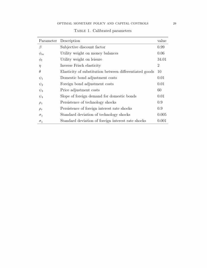
IV.2. Parameter calibration. The parameters to be calibrated include β, the sub-jective discount factor; φm and φl, the utility weights for real money balances andleisure; η, the inverse Frisch elasticity of labor supply; θ, the elasticity of substitu-tion between differentiated products; ψ1 and ψ2, the adjustment cost parameters fordomestic and foreign bonds; ψ3, the adjustment cost parameter for price setting; ψ4,the slope parameter in the foreign investor’s demand schedule for domestic bonds; ρzand ρr, the persistence parameters for the technology shock and foreign interest rateshock processes; and σz and σr, the standard deviations of the two shocks. Table 1displays the calibrated values of these parameters.

Since we have a quarterly model, the subjective discount factor β is set to 0.99,so that the steady-state real interest rate is 4 percent. Based on the money demand

11See also Woodford (2003).12Evaluating welfare requires second-order approximations because the model’s risky steady state

is in general different from the deterministic steady state (Kim et al., 2008; Coeurdacier et al., 2011).Our approach to evaluating welfare based on second-order approximations is similar to the approachused by Schmitt-Grohé and Uribe (2004), which takes into account of potential effects of the riskysteady state.


regression by Chari et al. (2000), we set Φm = 0.06. We set η = 2, so that the Frischelasticity of labor supply is 0.5, which is consistent with empirical studies Keane andRogerson (2011). We calibrate φl so that the steady-state labor hours are about 30percent of the time endowment The elasticity of substitution between differentiatedproducts is set to θ = 10, implying a steady-state markup of about 11 percent, whichlies in the range estimated by Basu and Fernald (1997). We set the price adjustmentcost parameter to ψ3 = 60, which is consistent with an average duration of pricecontracts of about three quarters, in line with empirical evidence on price rigidities(Nakamura and Steinsson, 2008).13 We have less guidance for calibrating the portfolioadjustment cost parameters. We set φj = 0.01 as a baseline (j ∈ {1, 2, 4}) and weexamine the sensitivity of our results for different values of these adjustment costparameters. For the shock parameters, we set the persistence to ρz = 0.9 and ρr = 0.9

and the standard deviations to σz = 0.005 and σr = 0.001.14

In all our numerical experiments below, we focus on a steady state equilibrium withzero inflation (i.e., π̄ = 1), no capital flow taxes (τ̄ = 0), no government holdings offoreign reserves (b̄∗g = 0), and with a ratio of trade balance to aggregate output of 2

percent.

IV.3. Optimal policy outcomes. We now discuss the optimal policy outcomes.In the benchmark case, we assume that the Ramsey planner optimally sets bothsterilized interventions (by varying the amount of foreign reserves) and capital accountrestrictions (by varying the tax rate on capital inflows) to maximize the social welfare,taking as given the private-sector’s optimizing decisions. We then consider threealternative regimes, each being a special case of the benchmark policy. In the firstregime, the planner optimally sets capital control policies but not sterilization policies.Thus, while the tax rate on capital inflows is adjusted optimally, the amount of foreignreserves is held fixed at the steady-state value (i.e., b∗gt = b̄∗g = 0). In the secondregime, the capital-inflow tax rate is held at the steady-state value (i.e., τt = τ̄ = 0),

13The slope of the Phillips curve in our model is given by κ ≡ θ−1ψ3

CY , where the steady-state ratio

of consumption to gross output is 0.98 (so that the steady-state trade balance to output ratio is 2percent, as in Mendoza (1991)). The values of θ = 10 and ψ3 = 60 imply that κ = 0.153. In aneconomy with Calvo (1983) price contracts, the slope of the Phillips curve is given by (1−βαp)(1−αp)

αp,

where αp is the probability that a firm cannot reoptimize prices. A slope of 0.153 for the Phillipscurve in the Calvo model implies that αp = 0.68 (taking β = 0.99 as given), which corresponds to anaverage price contract duration of about 3 quarters. The study by Nakamura and Steinsson (2008)shows that the median price contract duration is between 8 and 12 months.

14The qualitative results do not change for a reasonable range of these shock parameters.


while the foreign reserve position is optimally adjusted. In the third regime, both thecapital-inflow taxes and the foreign reserves are held at their steady-state values andtherefore neither capital controls nor sterilization is optimally set by the planner. Inthe third regime, the only instrument for the planner is domestic monetary policy (bychoosing either the nominal interest rate or the inflation rate).

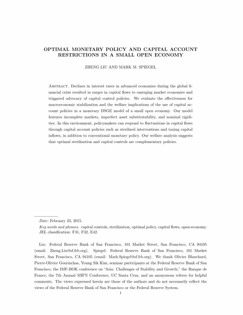
IV.3.1. Impulse responses. Figure 1 shows the impulse responses of macroeconomicvariables to an unexpected decline in the foreign interest rate in the benchmark case.The shock leads to a reduction in capital outflows and an increase in capital inflows.The balance of payments implies that the current account goes into deficit. The declinein foreign demand reduces aggregate output and inflation. Since the real exchangerate is constant under the law of one price, the decline in inflation corresponds to anominal exchange rate appreciation.

Optimal Ramsey policy calls for an easing of domestic monetary policy by reducingthe domestic nominal interest rate. Such policy easing helps alleviate the declinesin output and inflation. Optimal policy also calls for stabilization of the impact ofcapital flows through increased holdings of foreign securities and tightened capitalcontrols. To implement the latter, the government raises the tax rate on the returnsfor foreign investors. The combination of these capital account policies smoothesfluctuations in capital flows (e.g., the response of bft is close to zero). Furthermore,the increase in foreign reserves, combined with the decline in domestic bond supply,implies a large increase in money supply and thus a highly expansionary monetarypolicy. As a consequence, domestic consumption rises despite the fall in aggregateoutput, implying a large decline in the trade balance (not shown).15

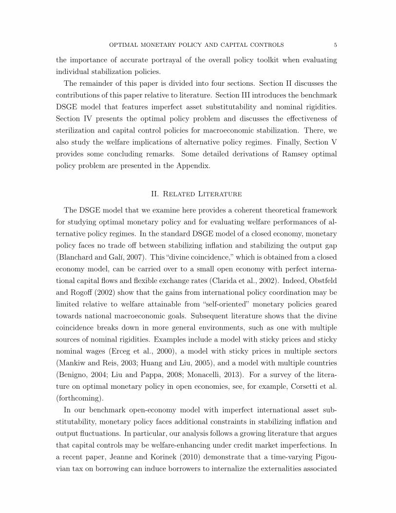
Figure 2 shows the impulse responses to an unexpected negative technology shock inthe benchmark case. Similar to that in the standard New Keynesian model, a declinein aggregate productivity reduces output and raises inflation. As inflation rises, theplanner tightens monetary policy by raising the nominal interest rate. However, theincrease in the nominal interest rate does not sufficiently compensate for the increasein inflation, leading to a decline in the real interest rate. With a lower real return,the demand for domestic bonds falls, resulting in a reduction in capital inflows and

15To keep our analysis tractable, our model has neither capital nor non-tradable goods. In a moregeneral model with investment, foreign interest rate declines may trigger capital inflow surges andcould lead to investment booms, potentially raising output and inflation. Nonetheless, we wouldexpect the sterilization and capital control policies that we consider here to be similarly useful forstabilization in these environments.


raising the scope for stabilization through sterilized intervention or capital controlpolicy adjustments. The planner therefore lowers the tax rate on foreign earnings andreduces its holdings of foreign reserves. Again, the planner is able to effectively insulatecapital inflows from the productivity shock (the impulse responses of bft is close tozero). At the same time, since the foreign interest rate does not change, the householddemand for foreign bonds does not change either.16 Thus, the overall capital outflowdeclines. The tightening of policy, coupled with the decline in aggregate productivity,leads to a persistent fall in consumption.

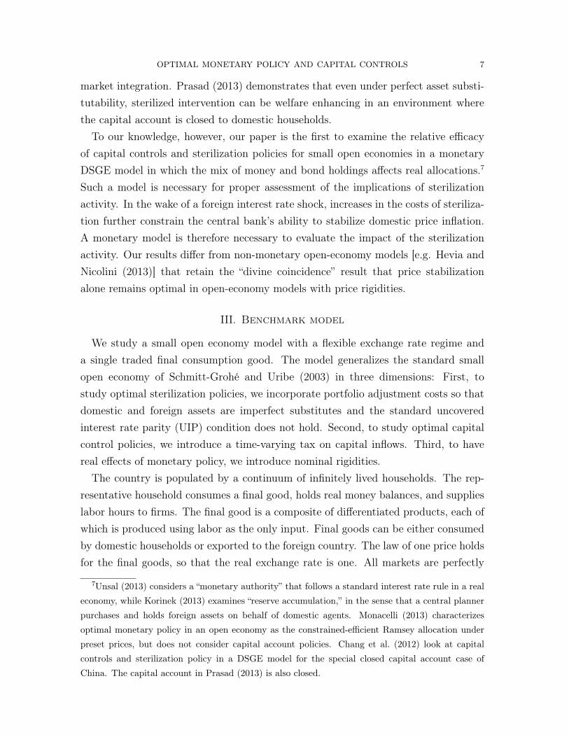
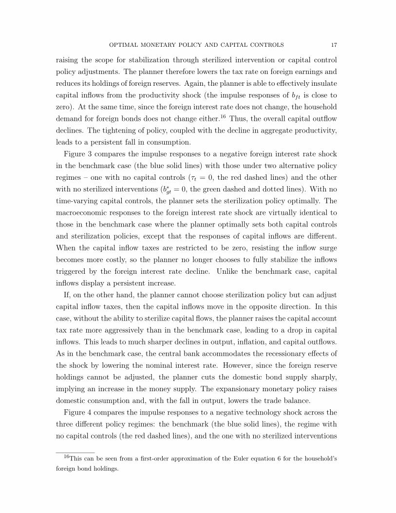
Figure 3 compares the impulse responses to a negative foreign interest rate shockin the benchmark case (the blue solid lines) with those under two alternative policyregimes – one with no capital controls (τt = 0, the red dashed lines) and the otherwith no sterilized interventions (b∗gt = 0, the green dashed and dotted lines). With notime-varying capital controls, the planner sets the sterilization policy optimally. Themacroeconomic responses to the foreign interest rate shock are virtually identical tothose in the benchmark case where the planner optimally sets both capital controlsand sterilization policies, except that the responses of capital inflows are different.When the capital inflow taxes are restricted to be zero, resisting the inflow surgebecomes more costly, so the planner no longer chooses to fully stabilize the inflowstriggered by the foreign interest rate decline. Unlike the benchmark case, capitalinflows display a persistent increase.

If, on the other hand, the planner cannot choose sterilization policy but can adjustcapital inflow taxes, then the capital inflows move in the opposite direction. In thiscase, without the ability to sterilize capital flows, the planner raises the capital accounttax rate more aggressively than in the benchmark case, leading to a drop in capitalinflows. This leads to much sharper declines in output, inflation, and capital outflows.As in the benchmark case, the central bank accommodates the recessionary effects ofthe shock by lowering the nominal interest rate. However, since the foreign reserveholdings cannot be adjusted, the planner cuts the domestic bond supply sharply,implying an increase in the money supply. The expansionary monetary policy raisesdomestic consumption and, with the fall in output, lowers the trade balance.

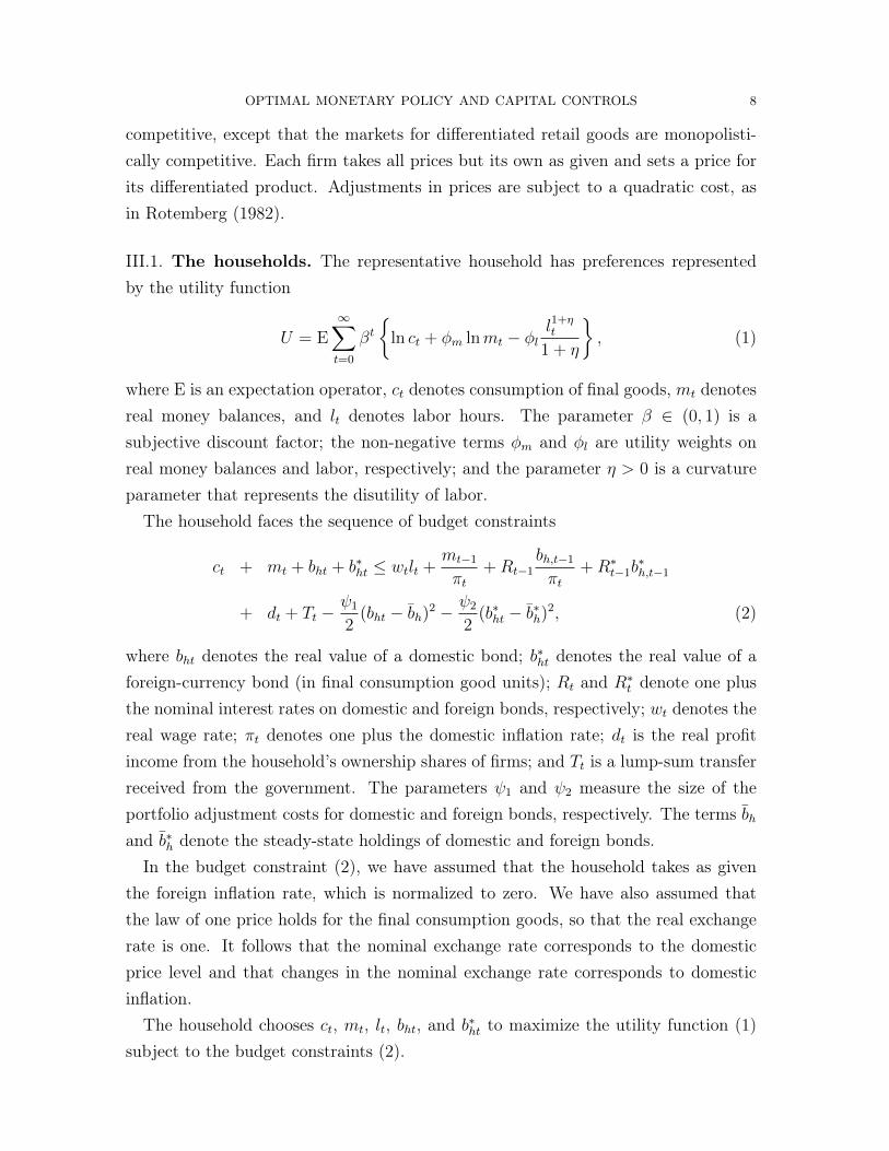
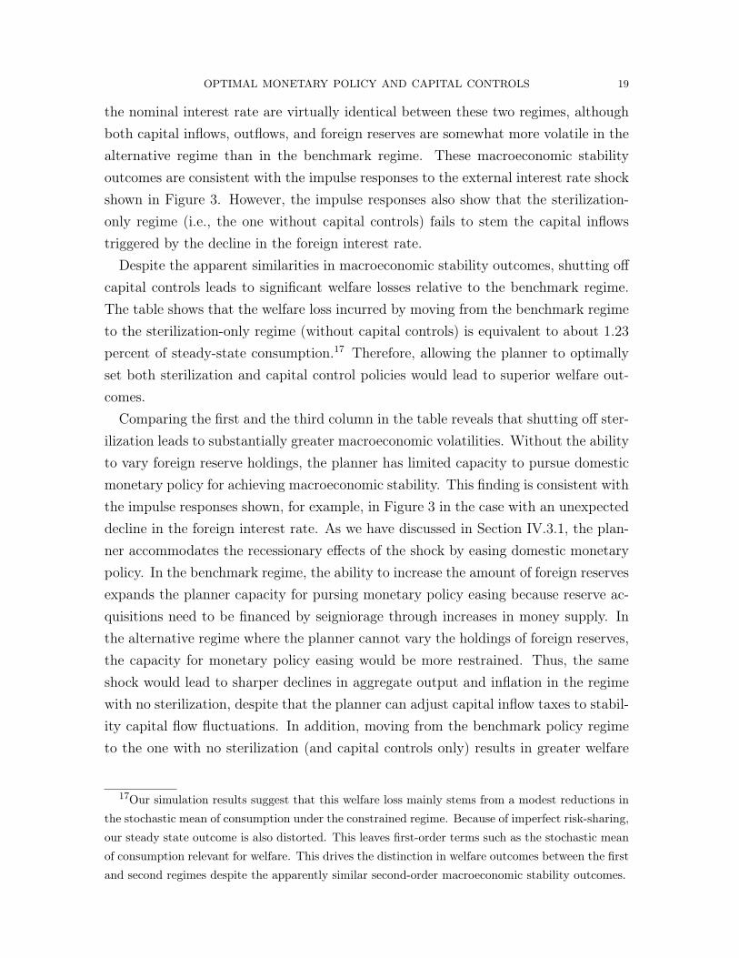
Figure 4 compares the impulse responses to a negative technology shock across thethree different policy regimes: the benchmark (the blue solid lines), the regime withno capital controls (the red dashed lines), and the one with no sterilized interventions

16This can be seen from a first-order approximation of the Euler equation 6 for the household’sforeign bond holdings.


(the green dashed and dotted lines). The differences of the impulse responses acrosspolicy regimes are broadly similar to the case with a foreign interest rate shock. Inparticular, the macroeconomic responses under the regime with no capital controlsare virtually identical to those in the benchmark regime, except that the responses ofcapital inflows are different. In the benchmark regime, the planner is able to smoothfluctuations in capital inflows by cutting the tax rate. When the taxes are restrictedto be zero, however, a negative technology shock leads to a decline in capital inflowsbecause the domestic real interest rate falls, as the inflation rate rises more than thenominal interest rate. In the case in which sterilized interventions are not pursued,the planner reduces capital inflow taxes more aggressively than in the benchmarkcase. As a result, the shock leads to an increase in capital inflows despite the declinein domestic real interest rates. Inflation also rises more than in the benchmark case,forcing the planner to tighten even more by raising the nominal interest rate. Thepolicy tightening along with the negative technology shock result in more persistentdeclines in consumption than in the benchmark case.

IV.3.2. Macroeconomic stability and welfare. Table 2 shows the macroeconomic sta-bility and welfare outcomes under the benchmark policy regime along with the threealternative regimes. These results are obtained with the economy exposed to bothtechnology shocks and foreign interest rate shocks. We evaluate welfare losses in termsof consumption equivalence for the three alternative regimes, i.e., how much additionalconsumption would be required to yield welfare comparable to the benchmark casewhere both sterilization and capital control policies are optimally set by the Ramseyplanner. Our model is sufficiently stylized that we would not stress the particularquantitative results. Instead, we focus on the qualitative results, which prove to beintuitive and helpful for understanding the implications of sterilization and capitalcontrol policies in our model framework.

The results for macroeconomic stability are consistent with the intuition from ouranalysis of the impulse responses. In particular, the results suggest that optimal ster-ilization policy is quite effective for stabilizing macroeconomic fluctuations driven bythe two types of shocks, while optimal capital control policy less so. To see this, wefirst compare the outcomes under the benchmark policy regime with both optimalsterilization and capital inflow taxes (the first column, under the title “Benchmark”)with those in the alternative regime where the planner is able to optimize over steril-ization policies but cannot vary the capital inflow tax rate (the second column, underthe title “No capital controls”). The volatilities of aggregate output, inflation, and


the nominal interest rate are virtually identical between these two regimes, althoughboth capital inflows, outflows, and foreign reserves are somewhat more volatile in thealternative regime than in the benchmark regime. These macroeconomic stabilityoutcomes are consistent with the impulse responses to the external interest rate shockshown in Figure 3. However, the impulse responses also show that the sterilization-only regime (i.e., the one without capital controls) fails to stem the capital inflowstriggered by the decline in the foreign interest rate.

Despite the apparent similarities in macroeconomic stability outcomes, shutting offcapital controls leads to significant welfare losses relative to the benchmark regime.The table shows that the welfare loss incurred by moving from the benchmark regimeto the sterilization-only regime (without capital controls) is equivalent to about 1.23

percent of steady-state consumption.17 Therefore, allowing the planner to optimallyset both sterilization and capital control policies would lead to superior welfare out-comes.

Comparing the first and the third column in the table reveals that shutting off ster-ilization leads to substantially greater macroeconomic volatilities. Without the abilityto vary foreign reserve holdings, the planner has limited capacity to pursue domesticmonetary policy for achieving macroeconomic stability. This finding is consistent withthe impulse responses shown, for example, in Figure 3 in the case with an unexpecteddecline in the foreign interest rate. As we have discussed in Section IV.3.1, the plan-ner accommodates the recessionary effects of the shock by easing domestic monetarypolicy. In the benchmark regime, the ability to increase the amount of foreign reservesexpands the planner capacity for pursing monetary policy easing because reserve ac-quisitions need to be financed by seigniorage through increases in money supply. Inthe alternative regime where the planner cannot vary the holdings of foreign reserves,the capacity for monetary policy easing would be more restrained. Thus, the sameshock would lead to sharper declines in aggregate output and inflation in the regimewith no sterilization, despite that the planner can adjust capital inflow taxes to stabil-ity capital flow fluctuations. In addition, moving from the benchmark policy regimeto the one with no sterilization (and capital controls only) results in greater welfare

17Our simulation results suggest that this welfare loss mainly stems from a modest reductions inthe stochastic mean of consumption under the constrained regime. Because of imperfect risk-sharing,our steady state outcome is also distorted. This leaves first-order terms such as the stochastic meanof consumption relevant for welfare. This drives the distinction in welfare outcomes between the firstand second regimes despite the apparently similar second-order macroeconomic stability outcomes.


losses than moving to the regime with no capital controls (and sterilization only), asshown in the table.

When both sterilization and capital controls are taken away from the planner’s pol-icy toolkit, the only policy instrument available for the planner would be domesticmonetary policy (e.g., by using the nominal interest rate as an instrument). Compar-ing the first and the last columns in Table 2 reveals that such an alternative regimewould result in greater macroeconomic volatilities and significant welfare losses rel-ative to the benchmark. Furthermore, the macroeconomic implications of this mostrestrictive capital account regime are similar to those in the regime with no steriliza-tion policy (with capital controls only). This last finding confirms that allowing theplanner to purse optimal sterilization policies helps achieve superior macroeconomicstability and welfare outcomes, with or without optimal capital control policies.

Finally, it is interesting to compare the welfare outcomes seen from shutting offthe capital controls policy from our benchmark case (i.e. moving from the first tothe second column) and that obtained from allowing capital control implementationunder an environment with both policies shut off (i.e. moving from column four tocolumn three). We observe almost no welfare gain from allowing capital controls inan environment that does not allow for sterilization policy. In contrast, we observe anon-trivial decline in welfare when shutting off capital controls policy alone relative tothe regime where both policies are allowed. The observed gains to the use of capitalcontrols in our model are therefore sensitive to the presence or absence of sterilizationpolicy. When the central bank can use sterilization, the gains from optimal capitalcontrols policy are shown to be non-trivial. This implies that the two types of stabi-lization policies are complementary. However, a model which shuts off this channelmight erroneously reach the conclusion that the stability gains from capital controlsare modest. It is therefore important to accurately depict the available set of policyoptions when assessing the stability contributions of any individual policy.18

V. Conclusion

This paper examines the effectiveness of sterilization and capital control policies instabilizing macroeconomic fluctuations in a small open economy. We compare welfareoutcomes when these policies are used in concert and in isolation. Imperfect asset

18Since our model is stylized and we focus on specific shocks and specific types of asset marketfrictions, the magnitude of relative welfare losses can be sensitive to the inclusion of other shocksand frictions in the model. We leave for future research to investigate the welfare implications ofcapital account policies in a model with more realistic frictions and a broader set of shocks.


substitutability in our model leads to distortions on capital flows. This distortioncreates a role for sterilization and capital control policies to improve welfare in theface of external shocks beyond the use of conventional monetary policies alone.

We find that these capital account policies play an important role in isolating thesmall open economy from external and domestic shocks. We also find that the wel-fare improvement associated with the introduction of either of these policies is muchgreater when the other policy is also being implemented. Thus, our results suggestthat sterilization and capital controls serve as complements, rather than substitutes.Our findings demonstrate the importance of correctly specifying the overall policytoolkit when evaluating the contributions of individual stabilization policies.


Appendix A. Derivations of the Ramsey optimal policy problem

In this appendix, we derive the Ramsey planner’s optimizing decisions. The plannermaximizes the welfare objective

Et

∞∑t=0

βt[ln ct − φl

l1+ηt

1 + η

], (A1)

taking as given the private sector’s optimizing decisions summarized below.φmctmt

= 1− βEtctct+1

1

πt+1

, (A2)

wt = φllηt ct, (A3)

1 + ψ1(bht − b̄h) = βEtctct+1

Rt

πt+1

, (A4)

1 + ψ2(b∗ht − b̄∗h) = βEt

ctct+1

R∗t , (A5)

wtZt

=θ − 1

θ+ψ3

θ

ctyt


(πt+1

π− 1) πt+1

π

], (A6)

bft = ψ4

[(1− τt)Et

Rt

πt+1

−R∗t], (A7)

b∗gt − R∗t−1b∗g,t−1 = bt −

Rt−1

πtbt−1 +mt −

mt−1

πt, (A8)

bt = bht + bft, (A9)

b∗t = b∗ht + b∗gt, (A10)

yt = Ztlt. (A11)

cat = b∗t − b∗t−1 −(bft −

bf,t−1πt

), (A12)

tbt = yt − ct −ψ1

2(bht − b̄h)2 −

ψ2

2(b∗ht − b̄∗h)2 −

ψ3

2

(πtπ− 1)2ct, (A13)

cat = tbt + (R∗t − 1)b∗t−1 − [Rt−1(1− τt−1)− 1]bf,t−1πt

, (A14)

To keep the Ramsey problem tractable, we further reduce the set of private op-timizing conditions by substituting out the six variables wt, bht, b∗ht, lt, cat, and tbt

using equations (A3) and (A9)-(A13). The private optimizing conditions can then bereduced to 7 equations.


The Lagrangian for the Ramsey planner’s optimal policy problem is given by

L = Et

∞∑t=0

βt{

ln ct − φll1+ηt

1 + η

λ1t

{1− β ct

ct+1

1

πt+1

− φmctmt

}λ2t

{βctct+1

Rt

πt+1

− 1− ψ1(bt − bft − b̄h)}

λ3t

{βctct+1

R∗t − 1− ψ2(b∗t − b∗gt − b̄∗h)

}λ4t

{θ − 1

θ+ψ3

θ

ctyt

[(πtπ− 1) πtπ− β

(πt+1

π− 1) πt+1

π

]− φl

yηt ct

Z1+ηt

,

}λ5t

{bt −

Rt−1

πtbt−1 +mt −

mt−1

πt− b∗gt +R∗t−1b

∗g,t−1

}λ6t

{ψ4

[(1− τt)

Rt

πt+1

−R∗t]− bft

}λ7t

{yt − ct −

ψ1

2(bt − bft − b̄h)2 −

ψ2

2(b∗t − b∗gt − b̄∗h)2 −

ψ3

2

(πtπ− 1)2ct+

R∗t−1b∗t−1 −

Rt−1

πt(1− τt−1)bf,t−1 − b∗t + bft

}} (A15)

The planner solves the optimal policy problem by choosing the 10 endogenousvariables summarized in the vector

Xt ≡ [ct,mt, πt, bt, bft, Rt, b∗t , b∗gt, yt, τt]

along with the 7 Lagrangian multipliers λjt for j ∈ {1, 2, . . . , 7}. The first-orderconditions are summarized below.

0 = 1− λ1t[φmctmt

+ Etβctct+1

1

πt+1

]+ Etλ2tβ

ctct+1

Rt

πt+1

+ Etλ3tβctct+1

R∗t − λ4tφlyηt ct

Z1+ηt

+λ4tψ3

θ

ctyt


(πt+1

π− 1) πt+1

π

]− λ7t

ψ3

2

(πtπ− 1)2

+

λ1,t−1ct−1ctπt− λ2,t−1

ct−1ct

Rt−1

πt− λ3,t−1

ct−1ctR∗t−1, (A16)

0 = λ1tφmctm2t

+ λ5t − βEtλ5,t+1

πt+1

, (A17)

0 = λ1,t−1ct−1ctπt− λ2,t−1

ct−1ct

Rt−1

πt+ λ4t

ψ3

θ

ctyt

(2πt − 1)πt −


λ4,t−1ψ3

θ

ct−1yt−1

(2πt−1 − 1)πt + λ5t

[Rt−1

πtbt−1 +

mt−1

πt

]−

λ6,t−1ψ4

β(1− τt−1)

Rt−1

πt− λ7tψ3

(πtπ− 1)πtct + λ7t

Rt−1

πt(1− τt−1)bf,t−1, (A18)

0 = −λ2tψ1 + λ5t − Etβλ5,t+1Rt

πt+1

− λ7tψ1(bt − bft − b̄h), (A19)

0 = λ2tψ1 − λ6t + λ7t[1 + ψ1(bt − bft − b̄h)

]− Etβλ7,t+1

Rt

πt+1

(1− τt), (A20)

0 = Etλ2tβctct+1

1

πt+1

− Etβλ5,t+1btπt+1

+ λ6tψ4(1− τt)Et1

πt+1

−

Etβλ7,t+1(1− τt)bft1

πt+1

, (A21)

0 = −λ3tψ2 − λ7t[1 + ψ2(b

∗t − b∗gt − b̄∗h)

]+ Etβλ7,t+1R

∗t , (A22)

0 = λ3tψ2 − λ5t + Etβλ5,t+1R∗t + λ7tψ2(b

∗t − b∗gt − b̄∗h), (A23)

0 = −φlyηtZ1+ηt

− λ4tηφlyη−1t ct

Z1+ηt

−

λ4tψ3

θ

cty2t

[(πtπ− 1) πtπ− β

(πt+1

π− 1) πt+1

π

]+ λ7t, (A24)

0 = −λ6tψ4EtRt

πt+1

+ Etβbftλ7,t+1Rt

πt+1

. (A25)

The Ramsey optimal policy solution corresponds to the solution to the 17 equa-tions (A2), (A4)-(A8), (A14), and (A16)-(A25) for the 17 variables including the 10variables in the vector Xt and the 7 Lagrangian multipliers for the Ramsey problem.

We solve the Ramsey problem with calibrated parameters. To evaluate welfareunder the Ramsey optimal policy, we solve the Ramsey problem by taking second-order approximations of all optimizing decisions around the Ramsey steady state.This approach takes into account the effects of shocks on the stochastic means of theendogenous variables, which are important for welfare calculations (Schmitt-Grohéand Uribe, 2004; Kim et al., 2008)


References

Backus, D. K. and P. J. Kehoe (1989): “On the Denomination of GovernmentDebt: A Critique of the Portfolio Balance Approach,” 23, 359–376.

Basu, S. and J. G. Fernald (1997): “Returns to Scale in U.S. Production: Esti-mates and Implications,” 105, 249–283.

Benigno, G., H. Chen, C. Otrok, A. Rebucci, and E. R. Young (2014): “Op-timal Capital Controls and Real Exchange Rate Policies: A Pecuniary ExternalityPerspective,” CEPR Discussion Paper No. 9936.

Benigno, P. (2004): “Optimal monetary policy in a currency area,” Journal of In-ternational Economics, 63, 293–320.

Bernanke, B. S. (2012): “U.S. Monetary Policy and International Implications,”Speech at the "Challenges of the Global Financial System: Risks and Governanceunder Evolving Globalization," A High-Level Seminar sponsored by Bank of Japan-International Monetary Fund, Tokyo, Japan.

Bianchi, J. (2011): “Overborrowing and Systemic Externalities in the Business Cy-cle,” American Economic Review, 101, 3400–3426.

Blanchard, O. J. and J. Galí (2007): “Real Wage Rigidities and the New Key-nesian Model,” Journal of Money, Credit, and Banking, 39, 35–65.

Calvo, G. A. (1983): “Staggered Prices in a Utility-Maximizing Framework,” 12,383–398.

Chang, C., Z. Liu, and M. M. Spiegel (2012): “Capital Controls and OptimalChinese Monetary Policy,” Federal Reserve Bank of San Francisco Working Paper2012-13.

Chari, V., P. J. Kehoe, and E. R. McGrattan (2000): “Sticky Price Models ofThe Business Cycle: Can The Contract Multiplier Solve The Persistence Problem?”Econometrica, 68, 1151–1180.

Clarida, R., J. Galí, and M. Gertler (2002): “Optimal Monetary Policy inOpen versus Closed Economies: An Integrated Approach,” American EconomicReview, 91, 248–252.

Coeurdacier, N., H. Rey, and P. Winant (2011): “The Risky Steady State,”American Economic Review: Papers & Proceedings, 101, 398–401.

Corsetti, G., L. Dedola, and S. Leduc (forthcoming): “Optimal Monetary Pol-icy in Open Economies,” in Handbook of Monetary Economics, ed. by M. Woodfordand B. Friedman, Elsevier.


Costinot, A., G. Lorenzoni, and I. Werning (2011): “A Theory of CapitalControls as Dynamic Terms of Trade Manipulation,” NBER Working Paper 17680.

Devereux, M. B. and A. Sutherland (2011): “Country Portfolios In Open Econ-omy MacroâĂ?Models,” Journal of the European Economic Association, 9, 337–369.

Devereux, M. B. and J. Yetman (2014a): “Capital Controls, Global LiquidityTraps, and the International Policy Trilemma,” Journal of Scandinavian Economics,116, 218–313.

——— (2014b): “Globalisation, pass-through and the optimal policy response to ex-change rates,” Journal of International Money and Finance, 49, 104–128.

Edwards, S. (1999): “How Effective Are Capital Controls?” Journal of EconomicPerspectives, 13, 65–84.

Erceg, C. J., D. W. Henderson, and A. T. Levin (2000): “Optimal MonetaryPolicy with Staggered Wage and Price Contracts,” Journal of Monetary Economics,46, 218–313.

Farhi, E. and I. Werning (2012): “Dealing with the Trilemma: Optimal CapitalControls with Fixed Exchange Rates,” NBER Working Paper 18199.

Fernandez-Arias, E. and P. J. Montiel (1996): “The Surge in Capital Inflowsto Developing Countries: An Analytical Overview,” The World Bank EconomicReview, 10, 51–77.

Galí, J. and T. Monacelli (2005): “Monetary Policy and Exchange Rate Volatilityin a Small Open Economy,” The Review of Economic Studies, 72, pp. 707–734.

Ghosh, A. R., M. S. Qureshi, J. I. Kim, and J. Zalduendo (2014): “Surges,”Journal of International Economics, 92, 266–285.

Hevia, C. and J. P. Nicolini (2013): “Optimal Devaluations,” IMF EconomicReview, 61, 22–51.

Huang, K. X. and Z. Liu (2005): “Inflation Targeting: What Inflation Rate toTarget?” Journal of Monetary Economics, 52, 1435–1462.

Jeanne, O. and A. Korinek (2010): “Managing Credit Booms and Busts: APigouvian Taxation Approach,” NBER Working Paper No. 16377.

Johnson, S. and T. Mitton (2003): “Cronyism and Capital Controls,” Journal ofFinancial Economics, 67, 351–382.

Keane, M. P. and R. Rogerson (2011): “Reconciling Micro and Macro LaborSupply Elasticities: A Structural Perspective,” NBER Working Paper 17430.

Kim, J., S. Kim, E. Schaumburg, and C. A. Sims (2008): “Calculating and UsingSecond-Order Accurate Solutions of Discrete Time Dynamic Equilibrium Models,”


Journal of Economic Dynamics and Control, 32, 3397–3414.Korinek, A. (2013): “Capital Controls and Currency Wars,” Manuscript, Universityof Maryland.

Kumhof, M. (2010): “On the Theory of Sterilized Foreign Exchange Intervention,”Journal of Economic Dynamics and Control, 34, 1403–1420.

Liu, Z. and E. Pappa (2008): “Gains from International Monetary Policy Coordi-nation: Does It Pay to Be Different?” Journal of Economic Dynamics and Control,32, 2085–2117.

Mankiw, N. G. and R. Reis (2003): “What Measure of Inflation Should a CentralBank Target?” Journal of European Economic Association, 1, 1058–1086.

Mendoza, E. (1991): “Real business cycles in a small-open economy,” AmericanEconomic Review, 81, 797–818.

Monacelli, T. (2013): “Is Monetary Policy in an Open Economy FundamentallyDifferent?” IMF Economic Review, 61, 6–21.

Nakamura, E. and J. Steinsson (2008): “Five Facts About Prices: A Reevalua-tion of Menu Cost Models,” Quarterly Journal of Economics, 123, 1415–1464.

Obstfeld, M. and K. Rogoff (2002): “Global Implications of Self-Oriented Na-tional Monetary Rules,” Quarterly Journal of Economics, 117, 503–35.

Olivier Blanchard, I. d. C. F. and G. Adler (2014): “Can Sterilized ForeignExchange Intervention Stem Exchange Rate Pressures from the Global FinancialCycle?” Mimeo, IMF.

Ostry, J. D., A. R. Ghosh, K. Habermeier, M. Chamon, M. S. Qureshi,

and D. B. Reinhart (2010): “Capital Inflows: The Role of Controls,” IMF StaffPosition note SPN/10/04, February 19.

Prasad, N. (2013): “Sterilized Intervention and Caital Controls,” Mimeo.Rey, H. (2013): “Dilemma not Trilemma: The Global Financial Cycle and MonetaryPolicy Independence,” Jackson Hole Economic Symposium, 285–333.

Rotemberg, J. J. (1982): “Sticky Prices in the United States,” 90, 1187–1211.Schmitt-Grohé, S. and M. Uribe (2003): “Closing small open economy models,”Journal of International Economics, 61, 163–185.

——— (2004): “Optimal Fiscal and Monetary Policy under Sticky Prices,” Journal ofEconomic Theory, 114, 198–230.

Unsal, D. F. (2013): “Capital Flows and Financial Stability: Monetary Policy andMacroprudential Responses,” International Journal of Central Banking, 9, 233–285.


Woodford, M. (2003): Interest and Prices: Foundations of a Theory of MonetaryPolicy, Princeton, New Jersey: Princeton University Press.


Table 1. Calibrated parameters

Parameter Description valueβ Subjective discount factor 0.99φm Utility weight on money balances 0.06φl Utility weight on leisure 34.01η Inverse Frisch elasticity 2θ Elasticity of substitution between differentiated goods 10ψ1 Domestic bond adjustment costs 0.01ψ2 Foreign bond adjustment costs 0.01ψ3 Price adjustment costs 60ψ4 Slope of foreign demand for domestic bonds 0.01ρz Persistence of technology shocks 0.9ρr Persistence of foreign interest rate shocks 0.9σz Standard deviation of technology shocks 0.005σz Standard deviation of foreign interest rate shocks 0.001


Table 2. Macroeconomic volatilities and welfare under alternative pol-icy regimes

Benchmark No capital No sterilization Neither controlscontrols nor sterilization

σy 0.00553 0.00553 0.00784 0.00784σπ 0.00260 0.00260 0.00598 0.00598σR 0.00115 0.00115 0.00053 0.00053σb∗ 0.15919 0.15920 0.07033 0.07032σbf 0 0.00001 0.00002 0.00001σb∗g 0.21028 0.21029 0 0στ 0.00147 0 0.00207 0Welfare loss – 1.2304 2.9437 2.9424

Note: The term σx denotes the standard deviation of the variable x, where x denotesaggregate output (y), domestic inflation (π), nominal interest rate (R), domesticholdings of foreign bonds (b∗), foreign holdings of domestic bonds (bf), foreignreserves held by the government (b∗g), and the tax rate on interest earnings by foreigninvestors on domestic bonds. The welfare loss under each regime is measured bysteady-state consumption equivalent relative to the benchmark regime.


0 10 20

Dev

. fro

m S

S

#10-3

-3

-2

-1

0

1Output

0 10 20

#10-3

-3

-2

-1

0

1Inflation

0 10 20

#10-4

-6

-4

-2

0Interest rate

0 10 20

#10-3

-10

-5

0

5Domestic bond supply

0 10 20

#10-3

-6

-4

-2

0Capital outflow (b*)

0 10 20

#10-17

-2

0

2

4Capital inflows (bf)

0 10 200

0.02

0.04

0.06

0.08Govt foreign reserves (b

g*)

Quarters0 10 20

#10-4

0

2

4

6

8Capital inflow tax

0 10 20

#10-4

-5

0

5

10Consumption

Figure 1. Impulse responses to a negative foreign interest rate shockunder optimal sterilization and capital control policies.


0 10 20

Dev

. fro

m S

S

#10-3

-2

-1.5

-1

-0.5

0Output

0 10 20

#10-4

0

1

2

3

4Inflation

0 10 20

#10-5

2

4

6

8

10Interest rate

0 10 20

#10-4

-10

-8

-6

-4

-2Domestic bond supply

0 10 20-0.02

-0.015

-0.01

-0.005


0 10 20

#10-18

-6

-4

-2

0


0 10 20-0.02

-0.015

-0.01

-0.005Govt foreign reserves (b

g*)

Quarters0 10 20

#10-5

-6

-4

-2

0Capital inflow tax

0 10 20

#10-4

-2.5

-2

-1.5

-1

-0.5Consumption

Figure 2. Impulse responses to a negative technology shock underoptimal sterilization and capital control policies.


0 10 20

Dev

. fro

m S

S

#10-3

-10

-5

0

5Output

BenchmarkNo capital controlsNo sterilization

0 10 20

#10-3

-6

-4

-2

0

2Inflation

0 10 20

#10-4

-6

-4

-2

0Interest rate

0 10 20-0.03

-0.02

-0.01

0

0.01Domestic bond supply

0 10 20-0.015

-0.01

-0.005


0 10 20

#10-5

-1

-0.5

0

0.5


0 10 200

0.02

0.04

0.06

0.08Govt foreign reserves (b

g*)

Quarters0 10 20

#10-4

0

5

10Capital inflow tax

0 10 20

#10-3

-1

0

1

2Consumption

Figure 3. Impulse responses to a negative foreign interest rate shockunder alternative policy regimes.


0 10 20

Dev

. fro

m S

S

#10-3

-2

-1.5

-1

-0.5

0Output

BenchmarkNo capital controlsNo sterilization

0 10 20

#10-3

-1

0

1

2Inflation

0 10 20

#10-4

0

0.5

1Interest rate

0 10 20

#10-3

-5

0

5

10Domestic bond supply

0 10 20-0.02

-0.01

0

0.01Capital outflow (b*)

0 10 20

#10-6

-1

0

1

2


0 10 20-0.02

-0.015

-0.01

-0.005

0Govt foreign reserves (b

g*)

Quarters0 10 20

#10-4

-3

-2

-1

0

1Capital inflow tax

0 10 20

#10-4

-6

-4

-2

0Consumption

Figure 4. Impulse responses to a negative technology shock underalternative policy regimes.

Monetary policy regimes and capital account restrictions in a small

Documents

Transcript of Monetary policy regimes and capital account restrictions in a small