Monetary Policy ReportMonetary Policy Report | May 2016 7 Specifically, global economic activity...
49
Monetary Policy Report May 2016
Transcript of Monetary Policy ReportMonetary Policy Report | May 2016 7 Specifically, global economic activity...

Monetary Policy ReportMay 2016

Monetary Policy Report May 2016

Monetary Policy Report May 2016 Online edition Publication date | May 2016 Central Bank of Argentina Reconquista 266 (C1003ABF) Ciudad Autónoma de Buenos Aires República Argentina Tel. | (54 11) 4000-1207 Web site | www.bcra.gob.ar Contents and edition | Economic Research Deputy General Management Publishing design | Institutional Relations and Corporate Image Management The contents of this report may be reproduced freely provided the source is acknowledged
For questions or comments please contact: [email protected]

Preface
In the words of its Charter, the Central Bank of the Republic of Argentina “has as its purpose the promotion
of monetary and financial stability, employment and economic development with social equity, to the extent
of its powers and within the policies adopted by the national government”.
This order in its mandates clearly identifies monetary stability as the priority aim of the Central Bank. For
this reason, attaining a low and stable level of inflation is the objective on which the principal policies of the
institution, and specifically monetary policy, must focus.
Notwithstanding the use of other more specific instruments to fulfill its remaining mandates – such as
financial regulation and supervision, exchange regulation and innovation in savings, credit and means of
payment instruments – the principal contribution that monetary policy can make so that the monetary
authority complies with all its mandates is to focus on its fundamental priority.
With low and stable inflation, financial institutions are better able to calculate their risks, which ensures
greater financial stability. When inflation is low and stable, manufacturers and employers enjoy increased
predictability so that they can invent, undertake, produce and hire, which promotes investment and
employment. Thanks to low and stable inflation, lower-income families are able to preserve the value of
their earnings and their savings, making it possible to achieve economic development with social equity.
The contribution of low and stable inflation to these objectives is never so evident as when it does not exist:
the flight from domestic currency can destabilize the financial system and lead to crisis, destruction of the
pricing system hinders productivity and the creation of genuine employment, and the inflation tax hits the
most vulnerable households and fosters wealth redistribution in favor of the wealthiest. Low and stable
inflation prevents all this.
In line with this vision, the Central Bank is working towards an Inflation Targeting regime. As part of this
new mechanism, the institution is starting to publish its Monetary Policy Report on a quarterly basis. This
report is similar to the quarterly reports issued by countries that have already adopted Inflation Targeting.
Its main purpose is to inform society of the Central Bank’s perception of recent inflation dynamics and how
it expects prices will develop, explaining in a transparent manner the reasons for its monetary policy
decisions.
Buenos Aires, May 9, 2016.

Contents
Page 5 | 1. Monetary Policy: Evaluation and outlook Page 6 | 2. International context Page 12 | 3. Economic activity Page 20 | 4. Prices Page 26 | Box 1 / Public utility tariff adjustments Page 27 | Box 2 / Retail price measurement methodology Page 29 | Box 3 / Exchange rate pass-through in Latin America: lessons from recent experience Page 31 | 5. Monetary policy Page 38 | Box 4 / Inflation Targeting: the international experience Page 40 | Box 5 / Savings and financial investments under a flexible exchange rate regime Page 41 | Box 6 / Interest rates and inflation Page 43 | Box 7 / Monetary policy interaction with the treasury Page 46 | Abbreviations and acronyms

Monetary Policy Report | May 2016
5
1. Monetary Policy: Evaluation and outlook The Central Bank is implementing its monetary policy so that within a reasonable time-frame it can reach an annual rate of inflation of 5%. As an interim target during a transition year towards the formal adoption of an Inflation Targeting mechanism as from 2017, the monetary authority is seeking to ensure that inflation for the rest of 2016 comes in at below current inflation expectations, reaching a level as close to 25% year-on-year as possible in December. The Central Bank also aims to have inflation expectations for 2017 down to fewer than 17% before the end of the year. Because of the statistical emergency, the Central Bank uses various indicators to monitor the inflationary dynamic. These indicators record a rise in inflation between the end of 2015 and the early months of 2016 from levels of around 25% year-on-year to levels of close to 35%. This increase in the rate of inflation has mainly been due to the sharp correction in relative prices that has taken place as a result of the expectation, and subsequent materialization, of a rise in the official exchange rate, and higher rates for various public utilities, for which prices had been lagging very severely, particularly in the metropolitan area. As a result, price levels, which had been rising at a monthly rate of approximately 2%, accelerated temporarily to a rate of around 4% in the December/February period and to close to 3% in March. Inflation in the metropolitan area is expected to be high in April because of the impact of various increases in the prices of regulated services, but various sources point to a reduction in the core inflation rate. In this context, the Central Bank has given its monetary policy a contractionary bias. As from the end of February it adopted the interest rate as its principal monetary policy instrument, setting its policy rate – the cut-off rate for 35-day LEBAC bills – at 37%, and later at 38%. At the beginning of May, following signs of a decline in core inflation in the month of April, it decided to lower that rate by 50 basis points to 37.5%, to limit an increase in the tight money bias in monetary policy. This policy contributed to contain the inflationary dynamic. First, price level acceleration was limited, considering the size of the corrections. Second, this acceleration does not appear to have had a negative impact on monthly inflation expectations, which even declined slightly to levels of around 1.5% for the third quarter. Meanwhile, activity levels, stagnated since the end of 2011, still showed no sign of recovery in the first quarter. Various activity indicators have shown a certain weakness in consumption, a mixed performance in the case of investment, and a strong recovery in foreign trade. Nevertheless, looking forward, various forecasts coincide in predicting an economic recovery as from the second half of the year, mainly as a consequence of the elimination of the distortions that weighed on various sectors, the regaining of access to voluntary international credit markets as from the agreement reached with the holders of public bonds in litigation, and the macroeconomic restructuring that is currently under way. The Central Bank will continue to monitor the macroeconomic situation, using its instruments with flexibility to achieve its inflation target of an annual 5%.

CENTRAL BANK OF ARGENTINA
6
2. International context
The international context provided Argentina with mixed results in the early months of 2016. On the one hand, the most significant variables affecting the country’s external sector, such as growth by its trading partners and commodity prices, recorded a weak performance in year-on-year terms, although with significant improvements in the margin in the case of agricultural goods prices. On the other, global financial conditions, significant in determining access to external financing and its cost for the country’s public and private sectors, remain extraordinarily favorable. 2.1 External demand Given the structure of Argentina’s exports, the variables of most relevance to the country’s external demand are the growth of its trading partners — particularly those to which Argentina exports manufactured goods— and international commodity prices —regardless of the countries to which they are exported. Increases in the prices of exported commodities have an impact on domestic economic activity because they provide an incentive to produce. Above all, , they have a positive wealth effect, and this stimulates domestic demand. Of course, this wealth effect can also be felt from the lower prices for imported goods; nevertheless, in the case of Argentina, primary goods have a much greater weight in the export basket than in the import basket (see Charts 2.1, 2.2 and 2.3).
2.1.1 Global and trading partner growth The outlook for global growth is critical for both the growth of Argentina’s main trading partners and the price of its exports. This outlook remained modest in the early months of 2016.
Chart 2.1 | Argentina. Exports by category (2015)
Primary products23%
Manufactures of vegetable and animal
origin41%
Manufactures of industrial origin
32%
Fuels and energy4%
Source: BCRA from INDEC data
Soybeans32%
Wheat8%
Corn23%
Rest37%
Chart 2.2 | Argentina. Exports of manufactured goods (2015)
Brazil20%
Euro zone11%
United States6%
Chile5%India
5%
Rest53%
Total manufactures
Industrial originAnimal and vegetable origin
Euro zone16%
India8%
Brazil6%
Vietnam5%
Chile5%
Rest60%
Brazil40%
United States
8%Switzerland
7%Canada
6%
Chile5%
Rest34%
Source: BCRA from INDEC data
Chart 2.3 | Argentina. Imports
58,892 62,31253,775 52,922
11,917
9,12811,343
11,4546,865
877
111.9108.8
98.9
52.4
34.4
0
20
40
60
80
100
120
0
20,000
40,000
60,000
80,000
100,000
2012 2013 2014 2015 Q1-16
US$/bblUS$ millions
Fuels Rest Brent price(right axis)
Source: BCRA from INDEC and Bloomberg data

Monetary Policy Report | May 2016
7
Specifically, global economic activity continued to expand at a modest rate, despite the significant stimuli implemented by the world’s leading central banks. Growth forecasts for 2016 and 2017 have been revised downward slightly since the end of 2015, standing at 2.7% and 3.1%, respectively. In 2016, advanced economies are expected to show lower dynamism compared with 2015 (1.7% vs. 1.9%), but a slight recovery is expected in emerging countries (4.6% vs. 4.4%; see Chart 2.4). In this context, growth by the group of Argentina’s main trading partners continued to underperform in relation to global growth and the levels of previous years, mainly because of the weakness of Brazil (see Chart 2.5). This trend is expected to persist in 2016, to then moderate considerably in 2017. Brazil, destination of 21% of Argentina’s manufactured goods1, is today the main head-wind
1 Share of Brazil as a destination for Manufactured Goods of Industrial Origin (MOI) and Manufactured Goods of Agricultural Origin (MOA) in 2015.
facing Argentina’s external demand. A further fall in GDP is expected this year, after systematic downward revisions following the decline recorded for 2015 of 3.8%. In the first quarter it is expected that the economy will have declined by 6% year-on-year) (y.o.y) and 0.8% seasonally adjusted (s.a.) compared with the previous quarter2. In the euro zone, the destination of 11%3 of the country’s manufactured exports, the growth forecast is 1.5% for 2016, similar to that for 2015. In the first quarter, the region grew by 0.6% s.a. compared with the previous quarter. To conclude, the U.S. economy, which receives 6% of Argentina’s manufactured goods4, will grow by a moderate 2.0% in 2016, below the 2.5% rate forecasted in December. The first quarter was weaker than expected, with growth up an annualized 0.5% compared with the previous quarter.
2.1.2 Multilateral real exchange rate In addition to the dynamism of its trading partners, there is another factor relevant to the external demand for Argentine goods, and that is their “purchasing power” for such goods, or from another point of view, the relative competitiveness of Argentina when it comes to penetrating their markets. This competitiveness is reflected in the Multilateral Real Exchange Rate (ITCRM). According to the recent evolution of the ITCRM, the Argentine economy has recovered competitiveness since December 2015, with a rise in the ITCRM of close to 30%. Needless to say, this was mainly due to the normalization and unification of the exchange market (see Monetary Policy section), but it was also influenced by an improvement in the real parity with Brazil, basically a product of the nominal appreciation of its currency (see Chart 2.6). In addition, the effective real rate of exchange recorded an increase, also influenced by the elimination or reduction of export duties5 and the
2 According to forecasts surveyed by FocusEconomics. 3 Share of the countries making up the euro zone as destinations of MOI and MOA in 2015. 4 Share of the United States as the destination of exports of MOI and MOA in 2015. 5 Decrees 133/2015 and 160/2015 and their amendments.
Chart 2.4 | Global. Economic growth
-6
-4
-2
0
2
4
6
8
10
Q1-08 Q1-09 Q1-10 Q1-11 Q1-12 Q1-13 Q1-14 Q1-15 Q1-16 Q1-17f
y.o.y. % chg.
Emerging economies
World
Advanced economies
Source: FocusEconomics f: forecast
2016f 2017f
1,7 1,9
4,6 5,1
2,73,1
2015
4,4
2,8
1,9
Chart 2.5 | World and Argentina’s main trade partners economic growth
-4
-3
-2
-1
0
1
2
3
4
5
6
7
Q1-08 Q1-09 Q1-10 Q1-11 Q1-12 Q1-13 Q1-14 Q1-15 Q1-16f Q1-17f
y.o.y. % chg.
World Argentina´s main trade partners
*Weighted by argentine exports´shares, totalizing 75%.Source: FocusEconomics, IMF, Datastream and INDEC f: forecast

CENTRAL BANK OF ARGENTINA
8
replacement of the Export Transaction Registers (ROE) by the Export Sales Affidavit (DJVE)6, which has facilitated foreign trade operations, improving export incentives (see Economic Activity section). 2.1.3 Commodity prices In the context of modest global growth, international commodity prices remained below their levels one year earlier. This behavior was also influenced by a widespread appreciation of the U.S. dollar and an abundant offer of such goods, with production at close to record levels and stock-consumption rations close to the highest levels for the last decade (see Chart 2.7 and 2.8). Nevertheless, in the year to date important improvements have been noted in the margin, driven by actions and expectations of a more relaxed monetary policy in leading economies (see sub-section 2.2). This development can be seen in the commodities price index (IPMP), published on a daily basis by the Central Bank since 21 April. The IPMP —which
6 Joint Resolutions 4/2015, 7/2015 and 7/2015 and their amend-ments.
reflects the development of the international prices of the main primary products exported by Argentina – has risen by 13.3% in the year to date. By category, agricultural products have risen 13%, metals were up 15% and oil increased 22% (see Chart 2.9).
Chart 2.6 | Multilateral (ITCRM) and bilaterals (ITCRB) real exchange rates
60
70
80
90
100
110
120
Jan-15 Apr-15 Jul-15 Oct-15 Jan-16 Apr-16
12-17-15=100
RER against Brazil RER against United States RER against China
RER against Euro zone REER
Source: BCRA from INDEC, Datastream, DEGCBA and DPESL data
Real depreciation
Real appreciation
Chart 2.7 | Multilateral dollar and commodity prices
0
25
50
75
100
125
150
175
200
225
76
82
88
94
100
106
112
118
124
130
Apr-04 Apr-06 Apr-08 Apr-10 Apr-12 Apr-14 Apr-16
Dec-05=100
Dollar multilateral exchange rate index
IMF commodity price index (right axis)
Source: Fed and IMF
Dec-05=100
Depreciation
Appreciation

Monetary Policy Report | May 2016
9
In the case of agricultural products, in the year to date there have been higher prices for soybean, wheat and corn (12.8%, 7.5% and 2.0%, respectively). The rise in soybean price has been due to the impact on the coarse grain harvest of heavy rainfall in March and April. Nevertheless, the significance of the price increase, combined with the fact that it is taking place in the context of a widespread rise in the prices of various different primary products, is expected to offset the effect from harvest losses, given the weight in the export basket of these products. Looking forward, the forecast for high global agricultural production for the 2015/16 cycle remains unchanged, implying an abundant global supply. According to futures contracts, however, the prices of leading grains will show moderate increases over the rest of the year, compared with those seen during April (see Chart 2.10). In year-on-year terms, average levels for 2016 will remain virtually constant in the case of soybean and corn
(at around US$343/tn and US$144/tn, respectively), and somewhat lower in the case of wheat (around US$169/tn). In the case of the price of Argentina’s imports, Brent crude oil has risen 21.9% since the beginning of 2016. Oil prices are expected to continue to recover during the rest of the year, although they will still be lower in year-on-year terms averaging US$41/bbl.
2.2 International financial markets: favorable to borrowing International financial markets began 2016 showing considerable volatility, but this trend has been significantly reversed in recent months (see Chart 2.11).
Chart 2.8 | Main grains. Stock-consumption ratio
0.0
0.1
0.2
0.3
0.4
0.5
1985/86 1990/91 1995/96 2000/01 2005/06 2010/11 2015/16*
stock-consumptionratio
Corn Soybean
Wheat Rice
Source: USDA *Apr-16 estimation
Chart 2.9 | Index of commodity prices (IPMP)
100
200
300
400
500
600
700
27-Apr-13 27-Oct-13 27-Apr-14 27-Oct-14 27-Apr-15 27-Oct-15 27-Apr-16
Dec-01=100
IPMP - Agricultural
IPMP metals
Crude oil (brent)
IPMP
Source: INDEC and Datastream
Soybean meal 19.5Soybean 15.1Corn 4.7Wheat 15.2Copper 4.4Aluminum 9.4Crude oil 21.1Soybean oil 8.1Steal 51.7Gold 17.5Beef -8.2Barley 13.3IPMP 13.7
Accum. % chg. 2016
Chart 2.10 | Oil and main grain prices
352.4
143.5163.3
42.3
347.2
145.3166.0
43.0
350.1
147.2
173.4
44.2
0
50
100
150
200
250
300
350
400
Soy Corn Wheat Brent
US$/tn.
Apr-16
Futures May-16
Average futures - rest of 2016
Source: Bloomberg
Chart 2.11 | Advanced economies. Stock indexes
80
85
90
95
100
105
110
Jun-15 Aug-15 Oct-15 Dec-15 Feb-16 Apr-16
S&P500 (United States)
EuroStoxx600 (Europe)
MSCI Global
Dec-14 = 100
Source: Bloomberg
CENTRAL BANK OF ARGENTINA
10
Prices of emerging market financial assets followed this pattern (see Chart 2.12). The aggregate for emerging market indexes (measured in dollars) went from recording sharp falls in 2015 to posting gains in the year to date. Sovereign risk premiums, which had risen in 2015, have fallen in the first few months of the year. Currencies, which depreciated strongly in January, have appreciated since then. This performance, particularly as regards the recovery, was mainly driven by a change in monetary policy actions and outlook in the world’s leading economies: faced by moderate economic growth and a persistence of deflationary risks, the leading developed nation central banks intensified their expansive monetary policies or delayed any return to contractionary policies (see Chart 2.13).
Indeed, inflation in the world’s leading economies remained well under control. Latest figures for year-on-year inflation in the United States and China have been very moderate (0.9% and 2.3%, respectively). In Japan and the euro zone, year-on-year price variations even fell into negative territory (-0.1% and -0.2%, respectively). In response to this situation, the Federal Reserve left its interest rate unchanged and forecasted more moderate increases than those predicted at previous meetings. The members of the Federal Open Market Committee (FOMC) forecast gradual rises for current and next year that will depend on both the evolution of the global context and the U.S. economy (with a focus on inflation and the labor market). Markets have also seen a reduction in the likelihood of new increases in interest rates during 2016, with futures contracts suggesting lower levels than those forecasted by FOMC members, although with volatility as new economic indicators are published (see Chart 2.14). In line with this situation, yields on U.S. government bonds continue at historically low levels (see Chart 2.15).
Chart 2.13 | Benchmark interest rate of monetary policy
-1
0
1
2
3
4
5
6
7
Q4-11 Q4-12 Q4-13 Q4-14 Q4-15 Q4-16f Q4-17f
%
China
Japan
Euro area
United States
Source: Datastream and FocusEconomics f: forecast
Chart 2.15 | U.S. Treasury notes yields
0.0
0.5
1.0
1.5
2.0
2.5
Jun-15 Aug-15 Oct-15 Dec-15 Feb-16 Apr-16
%
Treasury notes - 2 years
Treasuty notes - 10 years
Source: Bloomberg
Chart 2.14 | U.S. fed funds target forecasts of FOMC members and fed funds futures
0
0.5
1
1.5
2
2.5
3
3.5
Dec-16 Dec-17 Dec-18
%
Fed funds forecast median of FOMC members
Fed funds rate futures
Source: Bloomberg
Chart 2.12 | Financial assets prices of emerging markets
40
70
100
130
160
Jun-15 Sep-15 Dec-15 Mar-16
Dec-14=100
MSCI* EMMSCI* Latin AmericaBrazilArgentina
Stocks
Source: Bloomberg *Morgan Stanley Capital International
0
200
400
600
800
Sovereign debt- Perceived risk
EMBI+
EMBI+ Latin America
EMBI+ Brazil
EMBI+ Argentina
b.p.
100
125
150
175
200
Jun-15 Sep-15Dec-15Mar-16
Currencies
Emerging currencies index
Latin America
Brazil
Argentina
Dec-14=100
Depreciation
Appreciation

Monetary Policy Report | May 2016
11
Meanwhile, the European Central Bank cut its deposit rate by 10 basis points (b.p.), to -0.40%, and its refinancing and marginal lending facility rates to 0.0% and 0.25%, respectively. It also increased its asset purchase program from €60 billion to €80 billion monthly. Last, in January the Bank of Japan imposed a negative rate on excess bank reserves, while the Bank of China reduced its reserve requirement ratio by 50 b.p. in February. All these actions represent extraordinarily favorable financial conditions from the standpoint of access to financing. It coincides with the reduction in country risk and the reopening for Argentina of financial markets, a consequence of the change in government that took place in December 2015 and the normalization by the public sector of its debt with bondholders in litigation. The relaxation of external restrictions on public financing is of great significance, given the need and advisability of this sector to gain access to funds from abroad to implement a non-inflationary financing program in the framework of a gradual reduction in the fiscal imbalance.
This improvement in external borrowing conditions also extends to the private sector, a fact already reflected in the recent fall in the Corporate Emerging Markets Bond Index (CEMBI7; see Chart 2.16). Any decline in the yield on corporate bonds on foreign markets directly benefits companies with access to international financing. In addition, when such companies borrow abroad, they free up resources on the domestic credit market. The drop in the yield of bonds issued by Argentine corporations abroad also benefits companies that finance their investment out of retained earnings. This is because that yield is a good proxy for the cost of long-term capital that these companies use to determine the profitability of their projects.
7 The CEMBI is an index compiled by JP Morgan that follows the development of liquid bonds in dollars of companies in emerging markets. The CEMBI risk premium measures the surcharge on the yields of these bonds compared to US Treasur-ies and functions as the corporate equivalent of the sovereign risk premium measured by the EMBI+ (JP Morgan Emerging Market Bond Index).
Chart 2.16 | EMBI and CEMBI risk premiums for Argentina
300
450
600
750
900
1,050
1,200
1,350
Apr-10 Apr-11 Apr-12 Apr-13 Apr-14 Apr-15 Apr-16
Sovereing debt (EMBI)
Corporate debt (CEMBI)
basic points
Note: On 04-27-16 EMBI risk premium went up more than100 basic points due to technical factors (price corrections because of cupons that could not been collected since the middle of 2014).Source: Bloomberg

CENTRAL BANK OF ARGENTINA
12
3. Economic activity8 Towards the end of 2015 the economy was stalled, with output and private sector employment recording levels similar to those of 2011. Faced by this situation, the Government promoted a change in the focus of its economic policy with the aim to recover the path of growth. In the first quarter of the year the response of activity indicators varied, with weakness in consumption, mixed signs for investment, and a strong recovery in international trade flows. It is however expected that the measures that have been taken will begin to provide a boost to economic activity as from the second half of the year. Shored up by various factors, it is unlikely that this recovery will be adversely affected by the anti-inflationary bias of monetary policy.
8 Within the framework of the emergency in the National Statistical System (Decree 55/2016) declared in relation to the INDEC, at the time this report is being prepared there is insufficient statistical information for any detailed monitoring of economic activity and the labor market. As a result, use has been made of several partial indicators that are available, prepared by public and private bodies (the latter including indicators compiled and published by various business sector chambers).
100
110
120
130
140
150
Mar-06 Mar-08 Mar-10 Mar-12 Mar-14 Mar-16
2004=100
General Activity Index (IGA)
Private registered employment
Source: O.J.Ferreres and Ministry of Labor, Employment and Social Security
Chart 3.1 | Private employment and economic activity

Monetary Policy Report | May 2016
13
At the end of 2015 the Argentine economy showed signs of having stalled, according to the various partial indicators that the Central Bank analyzes to monitor economic activity. Output and private employment remained at levels similar to those of 2011 (see Chart 3.1) and trade volumes were significantly down on their peak levels (see Chart 3.2). In this context, the Government introduced changes to the system, in the understanding that this stagnation was caused by the restrictions placed on the purchase of foreign currency, a lagging exchange rate and high taxes and impediments to international trade, as well as the uncertainty generated by growing fiscal and monetary imbalances at a time during which access to international financial markets was blocked. The principal ingredients of the new macroeconomic regime were therefore the normalization and unifying of the exchange market (see Monetary Policy sub-section), the reduction or elimination of taxes on exports and the easing of trade restrictions (see subsection 3.1.3), announcement of a fiscal program –including cuts in subsidies to the private sector during 2016— the refocusing of monetary policy towards its basic objective of combating inflation (see Monetary Policy chapter) and the recovery of access to international markets. In this context there were mixed signs from the economy in the first quarter, and any clear indication of a recovery is unlikely to be seen in the second quarter. Nevertheless, it is expected that as from the second half of the year the measures that have been taken will begin to be reflected in positive activity levels.
3.1 The economy in the first quarter According to the Central Bank’s Activity Nowcast9, the output of goods and services has shown a slight improvement in the first quarter (0.8% year-on-year —y.o.y.— and o.5% when seasonally adjusted —s.a— see Chart 3.3). Other short-term economic indicators are sending out ambiguous signals, however: weakness can be observed in various consumption indicators, there is a mixed performance by investment, while international trade flows are showing strong recovery.
3.1.1. Weakness in consumption Several indicators have pointed to a drop in private consumption in the first quarter. Supermarket and shopping mall sales measured in real terms10 fell 4.8% seasonally adjusted (s.a.) and 6.4% s.a., respectively, compared with the previous quarter, and retail sales measured by CAME were down 2.4% s.a. (see Chart 3.4). Consumer-linked tax receipts (Value Added Tax—IVA— gross) fell 2.2% s.a.
9 The Nowcast is an early economic activity prediction methodology for the current quarter. It takes advantage of the wealth of data available from a large number of indicators published with a greater frequency than that of GDP data, and is updated as soon as new information becomes available. See http://www.bcra.gov.ar/Pdfs/Investigaciones/WP_69_2015e.pdf 10 Throughout this chapter use has been made of a combined index made up of the Consumer Price Index for Buenos Aires (IPCBA) and the San Luis Consumer Price Index (IPC-SL) as a deflator of the nominal variables.
Chart 3.2 | Quantity indexes for exports and imports
132,5
101,0
253,5
215,5
70
110
150
190
230
270
Mar-04 Mar-06 Mar-08 Mar-10 Mar-12 Mar-14 Mar-16
seasonally adjusted series, 3 months m.a.,
2004=100
Exports Imports
Source: BCRA from INDEC data
-15%
-24%
Chart 3.3 | Nowcast of economic activity
0,8%
-3,5
-2,5
-1,5
-0,5
0,5
1,5
2,5
3,5
4,5
5,5
Q1-14 Q2-14 Q3-14 Q4-14 Q1-15 Q2-15 Q3-15 Q4-15 Q1-16
y.o.y. % chg.
Average
Source: BCRA
CENTRAL BANK OF ARGENTINA
14
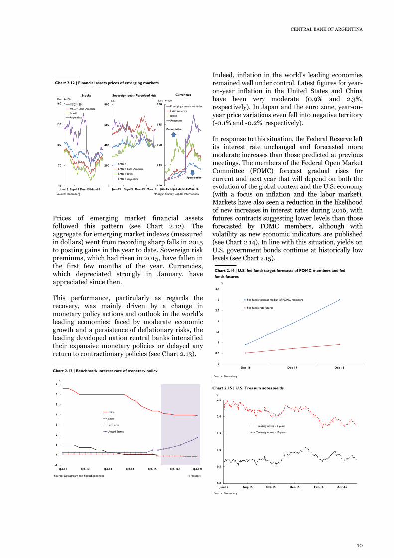
Certain indicators showed a more positive performance by household spending. Consumer goods imports picked up in the first three months of the year (14% y.o.y. and 3.3% for the quarter, s.a.; see Chart 3.5). Purchases abroad of vehicles were also up thanks largely to a boost from changes in taxation11, encouraging domestic market car sales, which rose 22.6% for the quarter s.a. (see Chart 3.6). Overall, the weakness in private consumption observed in the first quarter seems to have been influenced in part by the anticipation of spending that took place at the end of 2015. In addition, consumption was affected by the decline in real family income in the context of a temporary increase in the rate of inflation (see Prices chapter). According to the Federal Administration of Public Revenues (AFIP), nominal wage income rose 31% y.o.y. and employment was up 1.6% y.o.y. in the first quarter, in line with a real contraction
11 At the beginning of the year taxes on new car sales were modi-fied, with a rise in the tax-free minimum and a differentiated rate for locally-manufactured vehicles (Decree 11/2016).
of the wage mass of 0.9% y.o.y. in this sector. To a lesser extent, the behavior by private consumption could be linked to the anti-inflationary bias of monetary policy that could be encouraging greater saving by families. Public sector consumption has shown a neutral or slightly downward behavior during the first quarter of the year, influenced by the change in government and delays in executing certain budget items, reflected in a reduction in real terms of primary spending in the Non-Financial National Public Sector of around 5% y.o.y.
3.1.2. Mixed signals from investment Signals from investment indicators for the first quarter have been mixed. On the one hand, they suggest a recovery in investment in machinery and equipment. On the other, they mark a decline in construction. In the case of machinery and equipment, external purchases of capital goods and their parts and accessories measured in volume terms increased 2% y.o.y. and 15% y.o.y., respectively, although this was somewhat less than the year-on-year increases observed in the fourth quarter (see Chart 3.7).
Chart 3.5 | Vehicles and other consumer goods imports (volume)
Chart 3.4 | Short-term economic indicators: Private Consumption (volume)
-15
-10
-5
0
5
10
15
I-12 III-12 I-13 III-13 I-14 III-14 I-15 III-15 I-16
y.o.y. % chg.Retail stores Supermarkets* Shoppings* Real wage
Source: BCRA from INDEC, CAME, AFIP and DGEC-GCBA data *data up to feb-16
100
150
200
250
300
350
400
-60
-40
-20
0
20
40
60
I-12 I-13 I-14 I-15 I-16
2004=100y.o.y. % chg. Consumer goods
Vehicles
Level of consumer goods (s.a.; right axis)
Level of vehicles (s.a.; right axis)
Source: BCRA from INDEC data
Chart 3.6 | Vehicle production, sales and imports (in units)
-90
-60
-30
0
30
60
90
Q1-12 Q3-12 Q1-13 Q3-13 Q1-14 Q3-14 Q1-15 Q3-15 Q1-16
y.o.y % chg.External sales Sales in the internal market National production Imports
Source: BCRA from ADEFA data

Monetary Policy Report | May 2016
15
The recovery in flows of parts and accessories could have been brought forward in anticipation of a change in the system, already expected in 2015. Also, this recovery was probably encouraged by the easing of restrictions on foreign currency purchases and the elimination of impediments to trade as from December. In the case of construction indicators, cement shipments and the “Construya” index dropped 8.4% y.o.y. and 3.6% y.o.y. (5.6% s.a. and 17% s.a., respectively, compared with the previous period; see Chart 3.8). Employment in the sector was also down significantly (-3.4% y.o.y. in the formal segment according to AFIP data), as was domestic iron and steel output (17.8% y.o.y. and 17.3% y.o.y., respectively). Construction was probably affected by a combination of higher costs and a temporary fall in public works. Capital disbursements by the national public sector fell by more than 20 percentage points (p.p.) in real terms. This
significant drop could possibly have been due to a temporary phenomenon caused by ministerial reorganization and a review of the outstanding payments being claimed by related sectors. In general, the change in the focus of economic policy as a whole, including expectations of stabilization will probably have acted as a factor that will encourage investment in the long term. To a lesser extent, the anti-inflationary thrust of monetary policy could have a contractive impact on investment in the accumulation of inventory.
3.1.3. Rebound in exports and imports There have been strong signs of recovery in the external sector. Export volumes for goods increased 20% y.o.y. and 25% s.a. in the first quarter of the year, while import volumes rose 10% y.o.y and 2.7% s.a. There were various factors responsible for this performance. Exports in general benefitted from the normalization and unifying of the exchange market, which resulted in a more competitive exchange rate (see Chart 3.9; see Monetary Policy chapter). In addition, primary products and manufactured goods of agricultural origin (MOA) gained from the elimination or reduction of export duty rates and the elimination of impediments12 (see Chart 3.10). Although these measures
12 Joint Resolutions 4/2015, 7/2015 and 7/2015 eliminated the ROE register of export transactions and reintroduced the Export Sales Affidavits (DJVE), while Decree 133/2015 scrapped export duties on wheat and corn of 23% and 20%, respectively, and cut duties on the soybean complex by 5 percentage points, which in the case of soybean means a drop from 35% to 30%. In addition, restrictions on beef exports were eliminated and the US and Canadian markets were opened up, and it will now be possible to increase shipments to Russia and China.
Chart 3.7 | Investment indicators of capital goods
60
70
80
90
100
110
120
-60
-40
-20
0
20
40
60
Q1-12 Q3-12 Q1-13 Q3-13 Q1-14 Q3-14 Q1-15 Q3-15 Q1-16
y.o.y. % chg.Capital goods Parts and pieces
Level of capital goods (s.a.; right axis) Level of parts and pieces (s.a.; right axis)
Source: BCRA from INDEC data
2012=100
Chart 3.8 | Indicators of construction
-20
-15
-10
-5
0
5
10
15
Q1-12 Q3-12 Q1-13 Q3-13 Q1-14 Q3-14 Q1-15 Q3-15 Q1-16
s.a. m.o.m % chg.
Cement deliveries Construya Index
Source: BCRA from Grupo Construya and AFCP data
Chart 3.9 | Goods exports (quantities)
20
65
43
-17
-25
-40
-20
0
20
40
60
80
Total exports Primary products Agriculturalmanufactures
IndustrialManufactures
Energy and fuel
y.o.y. % chg. Q1-15 Q2-15 Q3-15 Q4-15 Q1-16
Source: BCRA from INDEC data

CENTRAL BANK OF ARGENTINA
16
probably encouraged a reduction in stocks, which had been at exceptionally high levels because of the effect of exchange market controls, they also appear to have acted as a stimulus to agricultural output (see sub-section 3.2). Export volumes of primary products, mainly grains, were up 65% y.o.y. in the first quarter (39% y.o.y. in value). MOA volumes rose 43% y.o.y., with an increase of 15% y.o.y. in export volumes. This performance was clearly reflected in certain production sectors, such as that of soybean milling, which grew 67% y.o.y. between January and March (see Chart 3.11). Exports of Manufactured Goods of Industrial Origin (MOI) fell 17% y.o.y. in volume, but the rate of decline was notably lower than that seen in the fourth quarter of 2015 (see Chart 3.12). The economic recession in Brazil has been a critical factor in the drop of MOI in recent years, particularly in the auto sector, as 73% of its exports are directed to that country. The rise in the exchange rate does however appear to have
moderated this headwind in the first few months of the year, as has the recent strengthening of the Brazilian currency. In the case of imports, all categories posted increases in the first quarter of the year, driven by the elimination of quantitative restrictions on trade, despite the fact that they could have been discouraged by the increase in the exchange rate. In volume terms, there were notable increases in purchases of passenger vehicles (53% y.o.y.), fuel and energy (39% y.o.y.), capital goods parts and accessories (15% y.o.y.) and consumer goods (14% y.o.y.). Purchases of intermediate and capital goods showed more moderate rises (1% and 2% y.o.y. respectively; see Chart 3.13). 3.2 Outlook for recovery First quarter indicators record a weak economic performance. In addition, according to the Leading
Charts 3.11 | Soybean crushing
0
1
2
3
4
5
jan feb mar apr may jun jul aug sep oct nov dec
2007 (47.5) 2008 (46.2) 2009 (30.9) 2010 (52.7) 2011 (48.9)
2012 (40.1) 2013 (49.3) 2014 (53.4) 2015 (61.4) 2016 (57.6)
million tonnes
Note: In the legend in brackets the relative production information for the cycle is presented Source: Ministry of Agro industry
Q1-16+67%
Chart 3.12 | Economic activity in Brazil and manufacturing exports
-15
-10
-5
0
5
10
15
20
-60
-40
-20
0
20
40
60
80
Q1-04 Q1-06 Q1-08 Q1-10 Q1-12 Q1-14 Q1-16
y.o.y. % chg.
Local production of vehicles
Industrial manufacture exports in quantities
Brazil economic activity (right axis)
Source: BCRA from INDEC and Brazil Central Bank data
y.o.y. % chg.
Chart 3.13 | Goods imports (quantities)
10
2 1
39
15 14
53
-60
-40
-20
0
20
40
60
Total imports Capital goods Intermediategoods
Fuels andlubricants
Parts andaccesories ofcapital goods
Consumptiongoods
Passengerautomotives
y.o.y. % chg. Q1-15 Q2-15 Q3-15 Q4-15 Q1-16
Source: BCRA from INDEC data
Chart 3.10 | Domestic and international grain prices
0.4
0.6
0.8
1.0
1.2
Jan-15 Apr-15 Jul-15 Oct-15 Jan-16 Apr-16
internal price/international price ratio
Wheat Corn Soybean
Source: BCRA from CBOT, MAGyP and MATBA data *data up to 20-apr

Monetary Policy Report | May 2016
17
Activity Indicator (ILA) prepared by the Central Bank 13 , there are as yet no clear signs of any recovery in the second quarter (see Chart 3.14). Nevertheless, the Central Bank expects to see a recovery in the Argentine economy as from the second half of the year, in line with forecasts from various sources (see Chart 3.15). These expectations are supported by various factors that are likely to impact, or will continue to impact, in a positive manner on economic activity. First, the comprehensive change that has taken place in economic policy has reduced the previously-existing levels of uncertainty and significantly improved agent expectations. The consumer confidence index prepared by the Torcuato Di Tella University reports optimistic expectations, despite certain moderation in recent months (see Chart 3.16). 13 The ILA, based on the methodology used by the Conference Board Leading Economic Index, is designed to anticipate possible changes in the domestic economic cycle. See https://www.conference-board.org/data/bci/index.cfm?id=2161
Second, the normalization and unifying of the exchange market are likely to continue to boost activity in various sectors, particularly in the case of tradable goods. The increased competitiveness of the exchange rate, added to the reduction and/or elimination of restrictions and taxes on exports, will no doubt continue to encourage exporting sectors and regional economies. Initial estimates indicate a 25% increase in the area sown with wheat for the 2016/17 season14. In addition, prospects for improved profitability will encourage greater investment in agrichemicals and high-technology farm machinery that will improve yields. In a similar manner, the livestock sector has in recent months seen a strong holding back of breeding cows from slaughter, a sign that beef farmers are planning to rebuild their cattle stocks (see Chart 3.17). Third, unrestricted access to the exchange market and the elimination of impediments to imports should continue to encourage a recovery in
14 Buenos Aires Grain Exchange report dated April 13, 2016.
Chart 3.14 | Leading indicator of economic activity (cycle component)
-30
-20
-10
0
10
20
30
Mar-05 Mar-06 Mar-07 Mar-08 Mar-09 Mar-10 Mar-11 Mar-12 Mar-13 Mar-14 Mar-15 Mar-16
Diffusion
Leader
General Activity Index (IGA)
Note: The cyclical component arises from applying the Christiano-Fitzgerald filter to the original series. Diffusion index represents the percentage of components with positive variations of Leader index.Source: BCRA from OJF, Industry associations, Bloomberg, AFIP and UTDT data
Chart 3.15 | Economic Growth Forecasts 2016 y 2017
-4
-2
0
2
4
Q1-16 Q2-16 Q3-16 Q4-16
y.o.y. % chg.
FocusEconomics
Bloomberg
3,2
2,8
2,9
3,0
1,9
-1,1
-1,0
-0,7
-0,5
0,7
Consensus Economics
IMF
FocusEconomics
Bloomberg
World Bank
2016 2017y.o.y. % chg.
Chart 3.17 | Cattle slaugher
38
40
42
44
46
48
-12
-6
0
6
12
18
Q1-13 Q3-13 Q1-14 Q3-14 Q1-15 Q3-15 Q1-16
y.o.y. % chg.
Female participation (right axis) Cattle slaughter
Source: BCRA from Ministry of Agroindustry and Instituto de Promoción de la Carne Vacuna data
%
Chart 3.16 | Consumer confidence index
0
10
20
30
40
50
60
70
80
Apr-12 Oct-12 Apr-13 Oct-13 Apr-14 Oct-14 Apr-15 Oct-15 Apr-16
points
Difference (expectations-current conditions)
Expectations
Current conditions
Source: UTDT
Optimism
Pesimism

CENTRAL BANK OF ARGENTINA
18
purchases abroad, which are essential for manufacturing activity (see Chart 3.18). Fourth, settlement of the litigation with bondholders has improved access and cost of external financing for the whole economy. In the case of the public sector, this will enable the financing of greater volumes of public works, although always within the limits of the fiscal consolidation process. For the private sector, this will mean external funding for major private corporations. In addition, it will help free up domestic market resources for borrowers without access to international financing and will encourage investments using own funds because of the lower opportunity cost of long-term capital (see International Context chapter). Fifth, the opening of the capital account together with the normalization of profit remittances abroad will lead to an increased inflow of Foreign Direct Investment (FDI). Latest available ECLAC15 data indicate that in 2014 FDI received by Latin America and the Caribbean totaled US$158.803 billion, of which only US$6.612 billion (that is to say, 4.2%) were directed to Argentina. FDI income in the region in 2014 represented on average 2.5% of GDP, while Argentina received only the equivalent to 1.2% of its GDP (see Chart 3.19). This means that FDI could more than double if the country converges on the regional average in terms of Product.
15 Economic Commission for Latin America and the Caribbean (ECLAC); “Foreign Direct Investment in Latin America and the Caribbean”, 2015, Santiago de Chile. A UN publication.
This having been said, certain factors could have a negative impact on aggregate demand. First, the temporary increase in prices could continue to have a negative impact on real household income, although this impact will probably be moderated by the wage adjustments that have been agreed and the social policies that have been implemented 16 . Second, the expected decline in economic activity in Brazil will continue to restrict the growth in exports of industrial manufactured goods, and thus the related sectors of industry. Last, it is probable that public consumption will be neither an expansion factor nor a factor restricting economic recovery, in line with the gradual fiscal reorganization being carried out by the Government. Similarly, it is expected that international prices of the main export commodities will remain relatively stable for the rest of the year. On balance, the prospects for economic recovery are encouraging, and its seems unlikely that they will be compromised by the anti-inflationary bias of monetary economy (see Table 3.1). In the long term, low and stable inflation contribute to sustained growth.
16 These include: social tariffs and preferential pricing for residential electricity and gas as long as there is a saving in consumption, increased family allowances and the inclusion of self-employed workers in the system, extension of the universe of beneficiaries qualifying for the Universal Child Allowance (AUH), a once-only subsidy for those collecting the minimum retirement and pension benefit, and the planned return to lower-income sectors of the VAT they have paid.
Chart 3.18 | Imports and economic activity
-60
-30
0
30
60
-15
-10
-5
0
5
10
15
Q1-05 Q1-06 Q1-07 Q1-08 Q1-09 Q1-10 Q1-11 Q1-12 Q1-13 Q1-14 Q1-15 Q1-16
y.o.y. % chg.y.o.y. % chg.Economic activity Industrial production Imported quantities (right axis)
Source: BCRA from OJF, FIEL and INDEC data
Chart 3.19 | Foreign Direct investments / GDP
2.1
1.2
2.1
2.72.8
2.5
0
1
2
3
4
prom. 2004-2007
2008 2009 2010 2011 2012 2013 2014
% Argentina Brazil Latin america and the caribbean average
Source: BCRA from ECLAC

Monetary Policy Report | May 2016
19
Box 3.1 | Short-term drivers of the economic activity
Ex
pans
ive
fact
ors
-Reduction of macroeconomic uncertainty
-High international liquidity
-Normalization of exchange market and increase of exchange competitiveness
-Reduction or elimination of export duties
-Elimination of quantitative restrictions on imports
-Normalization of turns of profits abroad and opening of the capital account
-Lowering the costs of access and reopening of international financial markets
-Moderate growth in the economies of our major trading partners
-Lower real household income by the transitory rise in the general price level
Factors with neutral impact
-International prices of major export products
-Fiscal policy
Containmentfactors

CENTRAL BANK OF ARGENTINA
20
4. Prices17
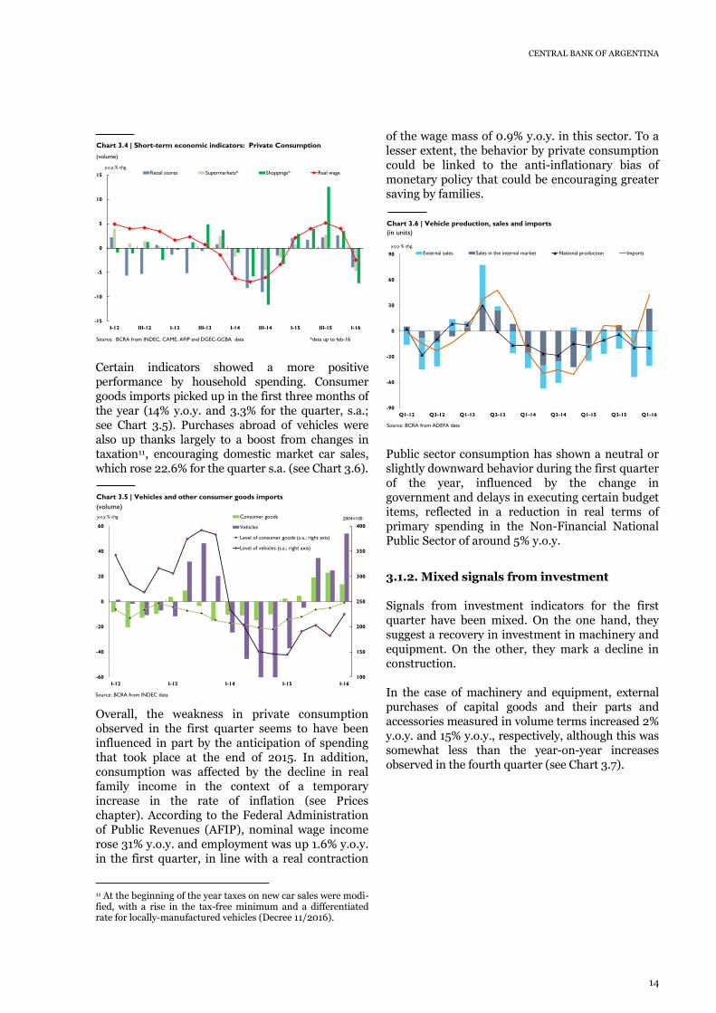
Various price indexes have shown an increase in inflation in the first quarter. Starting from levels of around 25% year-on-year of recent years, inflation has risen since the end of 2015 because of the expected, and subsequently materialized, increase in the official exchange rate, as well as because of the bringing up to date of various regulated prices that had been lagging, mainly in the Buenos Aires metropolitan region. Looking forward, although annual inflation expectations for the year to December are high, they predict a sharp drop in monthly inflation in coming months, which is already beginning to be seen in the underlying rate. The Central Bank will seek to lower inflation to below the level expected by the consensus for 2016, and reduce inflation expectations for 2017 to under 17%. All of this with the aim of moving towards an annual level of inflation of 5% in 2019. In recent years various retail price indexes have recorded rates of inflation in the order of 25% year-on-year (y.o.y.). The subordination of monetary policy to fiscal and exchange rate targets was the main reason for these high and persistent levels of inflation. Since the end of 2015 the rate of inflation has accelerated. The Consumer Price Index for the City of Buenos Aires (IPCBA) increased by a monthly 3.5% on average between November and March, consistent with an inflation rate of 35% y.o.y. at the end of the quarter. A similar performance was seen in consumer prices in San Luis (see Charts 4.1 and 4.2). This acceleration in prices was mainly the result of the anticipation and subsequent materialization of a sharp increase in the official rate of exchange as a consequence of the normalization and unification of the exchange market. To this were added other measures to improve the competitiveness of the tradable goods sector (see the International Context and Economic Activity chapters). In some districts, especially in the metropolitan area of Buenos Aires, an updating was also carried out in the case of various public services for which prices
had lagged considerably (see Box 1).
In line with this higher inflation there was also an increase in the expectations for annual average urban inflation by the end of the year, which rose from 31.8% last December to 33.4% in the latest measurement. The anti-inflationary bias of monetary policy has however helped contain the inflationary impact of the measures that have been adopted.
17 In the context of the emergency in the National Statistics System (Decree 55/2016), the Central Bank tracks the development of prices on the basis of various indicators that are available compiled by provincial statistical institutes, complementing the information with weekly surveys. Nevertheless, in this report the Central Bank will detail the development of prices by analyzing the Consumer Prices Indexes of the Province of San Luis (IPC-SL) and the Autonomous City of Buenos Aires (IPCBA). As informed by the INDEC (National Institute of Statistics and Census), both these indicators represent suitable alternatives to the Consumer Price Index in the absence of the index published by that Institute, as they both adopt methodologies that are mutually consistent, are based on their own representative baskets, and over the medium term show similar percentage variations. Recently the INDEC has informed that the official CPI for Greater Buenos Aires (GBA) will be published this June. The monthly variation corresponding to May will be reported in relation to the calculation for April 2016. Weightings will be based on the National Household Expenditure Survey (ENGH) corresponding to 2004-2005, although work is being carried out on the design of a new spending survey for 2017. It is also hoped to be able to count next year on an official index with a nationwide scope (see Box 2).
Chart 4.1 | Consumer price index. City of Buenos Aires and San Luis
0
5
10
15
20
25
30
35
40
45
50
Jan-07 Nov-07 Sep-08 Jul-09 May-10 Mar-11 Jan-12 Nov-12 Sep-13 Jul-14 May-15 Mar-16
y.o.y. % chg.
San Luis CPI
City of Buenos Aires CPI
Source: DGEC-GCBA, DPE-SL
Monetary Policy Report | May 2016
21
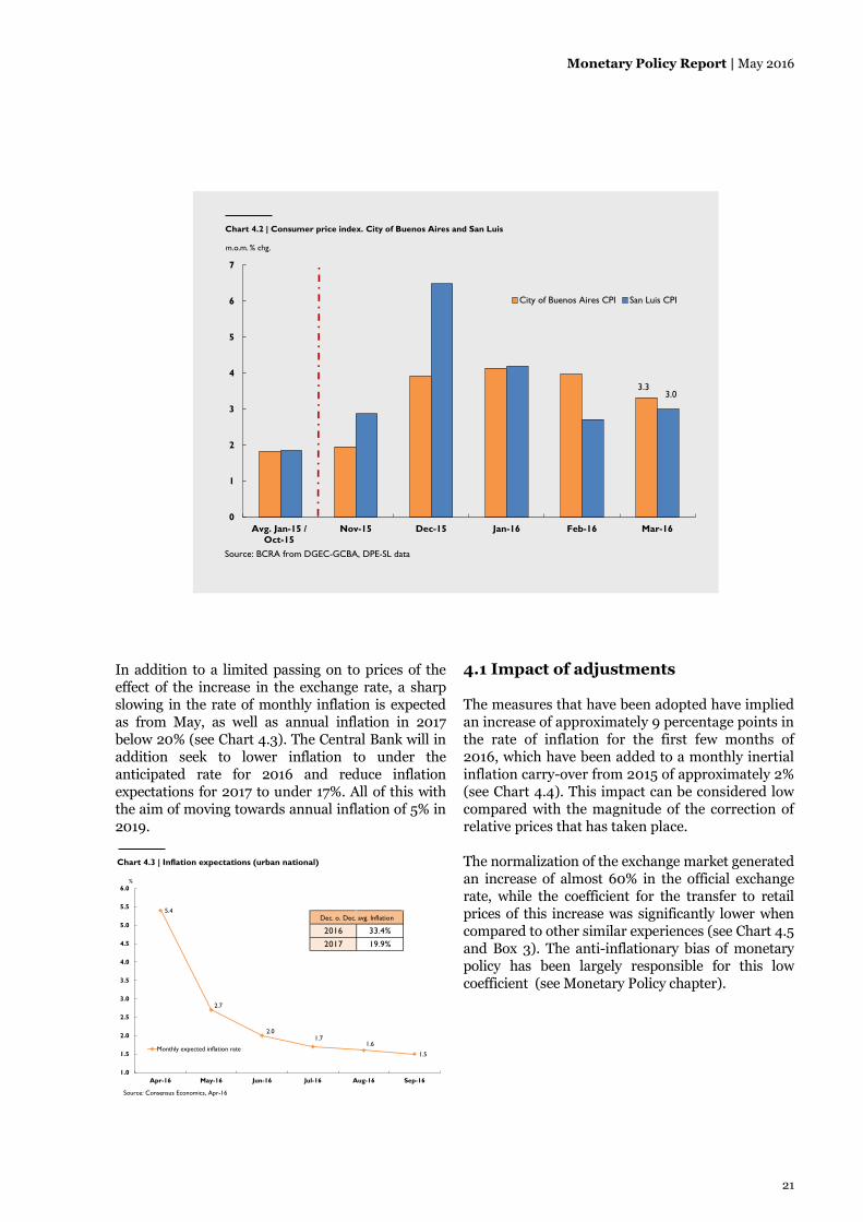
In addition to a limited passing on to prices of the effect of the increase in the exchange rate, a sharp slowing in the rate of monthly inflation is expected as from May, as well as annual inflation in 2017 below 20% (see Chart 4.3). The Central Bank will in addition seek to lower inflation to under the anticipated rate for 2016 and reduce inflation expectations for 2017 to under 17%. All of this with the aim of moving towards annual inflation of 5% in 2019.
4.1 Impact of adjustments The measures that have been adopted have implied an increase of approximately 9 percentage points in the rate of inflation for the first few months of 2016, which have been added to a monthly inertial inflation carry-over from 2015 of approximately 2% (see Chart 4.4). This impact can be considered low compared with the magnitude of the correction of relative prices that has taken place. The normalization of the exchange market generated an increase of almost 60% in the official exchange rate, while the coefficient for the transfer to retail prices of this increase was significantly lower when compared to other similar experiences (see Chart 4.5 and Box 3). The anti-inflationary bias of monetary policy has been largely responsible for this low coefficient (see Monetary Policy chapter).
Chart 4.2 | Consumer price index. City of Buenos Aires and San Luis
3.33.0
0
1
2
3
4
5
6
7
Avg. Jan-15 /Oct-15
Nov-15 Dec-15 Jan-16 Feb-16 Mar-16
m.o.m. % chg.
City of Buenos Aires CPI San Luis CPI
Source: BCRA from DGEC-GCBA, DPE-SL data
Chart 4.3 | Inflation expectations (urban national)
5.4
2.7
2.01.7
1.6
1.5
1.0
1.5
2.0
2.5
3.0
3.5
4.0
4.5
5.0
5.5
6.0
Apr-16 May-16 Jun-16 Jul-16 Aug-16 Sep-16
%
Monthly expected inflation rate
2016 33.4%
2017 19.9%
Dec. o. Dec. avg. Inflation
Source: Consensus Economics, Apr-16

CENTRAL BANK OF ARGENTINA
22
Chart 4.5 | CPI and nominal exchang rate. Pass-Through
In particular, its carry-over into construction costs was low. With a high participation by materials —goods that are sensitive to the exchange rate — construction costs accelerated in December but recorded a decline in their monthly rate of increase as from January (see Chart 4.6). In a similar manner, the retail prices of certain tradable goods for which additional measures were taken to improve their competitiveness (see Economic Activity chapter) did not fully
reflect increased producer prices. This is the case of the rises in the wholesale markets 18 for wheat, corn and beef, which have recorded increases of between 20% and 58% since December (see Chart 4.7).
18 As determined from the Buenos Aires Forward Market (MATBA) and the Liniers Cattle Market.
Chart 4.4 | Consumer price index. Evolution and linear trend
0.95
0.96
0.97
0.98
0.99
1.00
1.01
1.02
1.03
1.04
1.05
Mar-15 Jun-15 Sep-15 Dec-15 Mar-16
Nov-15 = 1Core City of Buenos Aires CPI
Core City of Buenos AiresCPI (ln)
Source: BCRA from DGEC-GCBA and DPE-SL data
Linear trend
Gap: 8,7%
0.95
0.96
0.97
0.98
0.99
1.00
1.01
1.02
1.03
1.04
1.05
Mar-15 Jun-15 Sep-15 Dec-15 Mar-16
Core San Luis CPI
San Luis CPI (ln)
Linear trend
Gap: 9,4%
Linear trendLinear trendLinear trend
3.4
4.74.0
2.6
4.5 4.13.0 3.0
11.3 11.4
0.8 0.9
18.319.5
8.7
0.8
29.7
34.2
50.3
59.0
24.421.1 22.3
28.0
0
20
40
60
80
0
4
8
12
16
20
Jan-14 Feb-14 Mar-14 Apr-14 Dec-15 Jan-16 Feb-16 Mar-16
ratio m.o.m. % chg.Core City of Buenos Aires CPI (a)
Nominal exchange rate (b)
Pass-Through (a/b accumulated; right axis)
Source: BCRA from DGEC-GCBA data
Chart 4.6 | Construction costs
2.6
2.0
1.1
4.8
0.8 1.0
2.0
5.1
3.0 2.8
1.0
18
22
26
30
34
38
0
2
4
6
8
10
Aug-15 Sep-15 Oct-15 Nov-15 Dec-15 Jan-16 Feb-16 Mar-16
%%
M.o.m. % chg. INDEC
M.o.m. % chg. CAC
Y.o.y. % chg. CAC (right axis)
Source: INDEC and CAC

Monetary Policy Report | May 2016
23
In the case of the increases in public utility prices, adjustments centered mainly on the metropolitan region of Buenos Aires – where rates showed the greatest lag. This change in relative prices between goods and services is being combined with an adjustment of prices on a geographical basis that has continued into the third quarter (see Table 4.1).
4.2 Analysis by region The City of Buenos Aires and San Luis price indexes went up by 12% and 10%, respectively in the first quarter. Although these increases were similar, the impact of their various components differed. In general terms, the increase in regulated service prices had a greater impact in the City of Buenos Aires, whereas in San Luis it was goods prices, and in particular food, that had the greatest impact. This was due in part to the mentioned tariff adjustments, but there was also an effect from differences in the consumer baskets, with food having a greater weight in San Luis.
In the City of Buenos Aires retail prices rose by 12% in the first three months of 2016, in line with an increase of 35% y.o.y. by the end of the period. Regulated services prices increased 18.4% in the quarter (accounting for 20% of the total increase), while the Seasonal CPI and Others CPI19 went up 11% in each case (see Chart 4.8). The “Housing, water, electricity and other fuels” component had the greatest impact, accounting for 20% of the rise in the general level accumulated in the year to date. In San Luis, almost 27% of the 10% rise accumulated in the first three months was explained by higher food prices, and between 13% and 14% in each case by the Transport and Communications, Leisure, and Housing and Basic Services headings (see Chart 4.9).
19 The “Others” category is a sub-basket that measures the change in prices of goods and services that do not have a seasonal compo-nent and are not subject to regulation, being a proxy for underly-ing inflation or so-called “core” inflation. Seasonal goods include fruit, vegetables, outdoor clothing, travel for tourism, lodging and excursions (General Directorate of Statistics and Census, Ministry of the Treasury, GCBA).
Chart 4.7 | Food prices
-10
10
30
50
70
90
110
130
150
Oct-15 Dec-15 Feb-16
y.o.y. % chg. Food wholesale prices
Wheat(MATBA*)Corn(MATBA*)Beef index**(Liniers)
-10
10
30
50
70
90
110
130
150
Oct-15 Nov-15 Dec-15 Jan-16 Feb-16 Mar-16
y.o.y. % chg. Food retail pricesBaked goods andcerealsBeef
Oil
*Mercado a Términos de Buenos Aires. **Mercado de Liniers beef indexSource: DGEC-GCBA, MATBA and Mercado de Liniers
Table 4.1 | Estimated incidence of tariffs on City of Buenos Aires CPI. 1Q-16 accumulated.
Item
Incidence(in p.p.)
Gas 2.13
Electricity 1.35
Urban transport 1.31
Water 0.83
Fuel 0.45
Taxi 0.29
Train 0.05
Cigarettes 0.09
Total 6.5Source: BCRA from DGEC-GCBA data
Chart 4.8 | City of Buenos Aires CPI. Regulated, seasonal and core goods and services
3.23
2.342.74
0.71
0.14
0.18
0.20
1.49 0.40
4.143.97
3.32
0
1
2
3
4
5
Jan-16 Feb-16 Mar-16
contribution to m.o.m. % chg. in p.p.
Regulated
Seasonally
Core
Source: DGEC-GCBA
Chart 4.9 | San Luis CPI. Incidence by components
4.2
2.7
3.0
0.0
0.5
1.0
1.5
2.0
2.5
3.0
3.5
4.0
4.5
Jan-16 Feb-16 Mar-16
contribution tom.o.m. % chg. in p.p.
Food & beverages Housing
Recreation Transport and communications
House eq. and maint. Apparel
Education Other goods and services
Health
Source: BCRA from DPE-SL data

CENTRAL BANK OF ARGENTINA
24
4.2.1 Significance of the “Other” category Analysis of inflation broken down into its constituent parts enables a more precise assessment of the underlying inflationary dynamic. In effect, in addition to monitoring indicators of the general level of inflation, the Central Bank carefully evaluates the development of indicators that do not consider transitory price changes, whether for seasonal reasons or because of once-only increases in public utility tariffs. These indicators are known as “underlying” or “core” indexes, or in the case of the City of Buenos Aires, IPC Resto or the CPI “Others” index. In the City of Buenos Aires a decline was recorded in the CPI “Others” index in the February-March two-month period compared with the December-January period, but even so its level was higher than the Central Bank would have wished (see Chart 4.10). Nevertheless, in April various public and private sources monitored by the monetary authority continue to record a further decline in core inflation. 4.3 Wages Approximately 70% of waged workers are registered, and 53% have their wages set by means of collective bargaining agreements (see Chart 4.11). Negotiations announced to date, involving over 30% of all workers covered by collective bargaining, have concluded with increases of between 15% and 24% in the case of agreements for six months and 28-22% in the case of annual agreements (except for workers in the vegetable oil sector, who negotiated a 38% increase, see Table 4.2).
4.4 Outlook Coming quarters will probably record a marked reduction in monthly inflation. The anti-inflationary bias of monetary policy would appear to be having some success in containing the second round effects of relative price adjustments on the inflationary dynamic. Although the annual inflation recorded in the first quarter and the expected inflation for the year to December 2016 are both high, inflation expectations for December 2017 are anchored at slightly below 20%. According to the survey that the Latin American Consensus Forecasts (LAC) performs among specialized analysts, a clearly downward path can be expected for monthly inflation as from May 2016.
Chart 4.10 | City of Buenos Aires. Core CPI
2.0 2.0 2.0 2.02.2
4.5
4.1
3.0
3.5
0.0
1.0
2.0
3.0
4.0
5.0
Q1-15 Q2-15 Q3-15 Oct-15 Nov-15 Dec-15 Jan-16 Feb-16 Mar-16
avg. m.o.m. % chg.
Soruce: DGEC-GCBA
Chart 4.11 | Formal private sector workers under collective wage agree-ment
52.7%47.3%
Total workers of the formal private sector: 6,581 million
Source: Ministry of Labor, employment and social security
4.3%5.0%
27.0%
12.9%6.5%
8.4%
8.7%
27.2%
Alimentation Truck drivers Trade
Construction Gastronomic Metallurgical
Health Other
Under collective
agreement
Without collective
agreement
Table 4.2 | 2016 wage agreements
Union
% of total agreement 3
Period Fixed sumRenegociation clause
2016
Oil producers
(FTCIODyARA) 38Apr-16/Mar-17
- -
Oct-15/Sep-16 - -
20% Oct-15/Nov-15 / 28% from Dec-15 - -
Bank workers (AB) 33 Jan-16/Dec-16 - √
Public transport (UTA)2
29Abr-16/Mar-17
$3.500 in 2-times fee √
Beef industry workers
(FGPICD) 20Apr-16/Sep-16
$2.000 in 6-times fee
Construction (UOCRA) 22 Apr-16/Sep-16 -
Trade and commerce20
Apr-16/Sep-16$2.000 in 2-times fee
Oil station workers 17 Apr-16/Sep-16 $1.480 in 2-time fee
Apr-16/Sep-16
20% Apr-16/Jul-16 and
3.33% since Aug-16
Jan-16/Jun-16
10% Jan-16/Feb-16 and 15% since Mar-16
Jan-16 / Jun-16
7.5% Jan-16/Mar-16 and 11% since Apr-16
(3) The agreement fee does not include fixed sums
Source: Journalism and union press information
Automotive (SMATA) 19 -
(1) Preliminar information, not yet published by Ministry of labor, employment and social security
(2) The agreement was signed for short and medium distance drivers
Sport and civil soc.
organizations
(UTEDyC)
15 -
Plastic producers (UOYEP) 24 $5.000 in 3-time fee
Semestral agreements 2016
Anual agreements 2016
Rural workers (UATRE) 28

Monetary Policy Report | May 2016
25
Since January, on average the consultants surveyed have been estimating that by June inflation will slow to a monthly 2%. These projections have not increased following the one-off increases in public utility tariffs announced in recent months – with an impact on the IPCBA of almost 7 percentage points in the first four months. On the contrary, they estimate that country-wide inflation will drop to 1.5% in September (see Chart 4.12).
With its monetary policy, the Central Bank is looking to have inflation follow a path that is lower than those expectations. The signs of a marked decline in core inflation in April suggest that this monetary policy is beginning to show results.
Chart 4.12 | 6-months expected inflation rate
3.8
3.0
2.32.1
1.91.7
5.4
2.7
2,0
1.71.6 1.5
1.0
1.5
2.0
2.5
3.0
3.5
4.0
4.5
5.0
5.5
6.0
Nov-15 Dec-15 Jan-16 Feb-16 Mar-16 Apr-16 May-16 Jun-16 Jul-16 Aug-16 Sep-16
m.o.m. % chg.
Nov-15
Dec-15
Jan-16
Feb-16
Mar-16
Apr-16
Source: Latin American Consensus Forecast, DGEC-GCBA, DPE-SL
LA Consensus Forecast monthly publication

CENTRAL BANK OF ARGENTINA
26
Box 1 / Public utility tariff adjustments Within the process for correction of the fiscal imbalance, which has required cuts in subsidy levels, the Government has ordered a series of increases in the prices of public utilities. First, it announced20 an increase in the seasonal reference price for wholesale electricity in February. This price is used to set rates for users obtaining their supplies through a distributor. As this tariff component is common to all the country’s consumers, the measure had a nationwide impact. The announcement established a differential adjustment between industries not registered as Wholesale Electricity Market (MEM) agents on the one hand, and traders, small industries and residential users, on the other. The adjustment not only meant an increase in wholesale prices but also a rise in costs in the various stages of the chain of production. In the Buenos Aires metropolitan area (AMBA) an additional increase was ordered for the added value of distribution 21, so that the average increase in the electricity tariff for that region was 250%, higher than the increase at national level. This increase had an impact on the Consumer Price Index for the City of Buenos Aires (IPCBA) of 1.3 percentage points in the month of February. As from April, increases were implemented nation-wide for natural gas network carrying and distribution costs, with differentiated percentages according to region and user category (classified by level of consumption)22. These increases were in addition to the rise in the price to producers of gas at Point of Entry to the Carrying System (PIST)23. In the case of residential users in the AMBA benefitting from a subsidy – almost 85% - rates rose by a minimum 144% for the R34 category (two-month consumption in excess of 1,800 cubic meters) and a maximum of 313% for R31, for two-monthly gas consumption of up to 500 cubic
20 Resolution 6/2016 issued by the Ministry of Energy and Mining. 21 Resolution 1/2016 issued by the National Electricity Regulator (ENRE). 22 Resolutions from 3723/2016 to 3733/2016 issued by the National Gas Regulator (ENERGAS) 23 Resolution 28/2016 issued by the Ministry of Energy and Mining.
meters). As a result, the rate has risen by an average of close to 195%. It should be noted that at the same time as the tariff change, the charge to cover the cost of imported gas in force since 2008 was eliminated, helping to soften the impact of the increase. A new rate schedule was also established for the drinking water and sewerage services in the AMBA provided by Agua y Saneamientos Argentinos S.A. (AySA)24. Calculation of the new tariff continues to use the same formula, but the value of the coefficient applied to determine the variable charge has been increased by 217%. In addition, the percentages applied to set preferential rate were lowered. Overall, the average increase will be close to 300%. Last, as from April 8 new fares came into force for urban bus and train services in the AMBA area of 100% in each case, with an impact in April of 65% and 60% respectively, with the remainder being applied in May25. It should be mentioned that in all cases the new tariff schemes include a social tariff for lower-income sectors, while in the case of electricity and gas, preferential prices are based on certain levels of savings in consumption. On the basis of the rises in the AMBA, it is estimated that the tariff adjustments will mean a floor for inflation of around 5% in April.
24 Provision 62/2016 issued by the Ministry of the Interior, Public Works and Housing. 25 Resolutions 46/2016 to 50/2016 issued by the Ministry of Transport.

Monetary Policy Report | May 2016
27
Box 2 / Retail price measurement methodology The Consumer Price Index —CPI— measures changes over time in the general price level of goods and services purchased by households for consumption. In many countries these indexes appeared to measure the cost of living of salaried workers, with the aim of adjusting salaries on the basis of price rises. Over the years, with the progress made in index number statistics, CPIs have broadened their scope, and today they are used as macroeconomic inflation indicators. Governments and central banks use them to monitor price stability, so that awareness of their methodological aspects is important. The most relevant price index from an economic standpoint is the one that is able to measure with precision the changes in the cost of living of consumers (the Cost of Living Index —COL)26. This makes it possible to determine the monetary income necessary to maintain a given level of welfare or satisfaction over time. The index number formulas that are the closest approximation to the COL are the so-called superlative indices that treat prices and quantities of all products consumed symmetrically and combine them, and are approximations to flexible functional forms of the underlying utility functions of consumers. These indices require information on the current period and the period with which they are being compared, which in practice makes it impossible for them to be published monthly27. For practical reasons, and to be able to calculate a price index that can be published on a regular basis, usually monthly, Laspeyres-type formulae are used to prepare the CPI. These indices, the origin of which dates back to the 18th century, provide timely information on the inflation rate, and are therefore used for a broad range of
26 This concept was introduced at the beginning of the 20th century. See “Consumer Price Index Manual – Theory and Practice”; International Labor Office (ILO), International Mon-etary Fund (IMF), Organization for Economic Cooperation and Development (OECD), Eurostat , United Nations (UN) and World Bank (WB), 2004. 27 These indexes assume that the preferences of individuals are homothetic, in other words, that changes in the income of indi-viduals do not affect the fraction they allocate to each product. There are three superlative indices that are widely used in eco-nomic statistics: Törnqvist or Törnqvist-Theil, Walsh and Fish-er. The latter is calculated as geometric mean between a Laspeyres index and a Paasche index.
purposes, including their use as a target in Inflation Targeting regimes. The exact way a CPI is defined and constructed largely depends on its intended purpose and who it will be used by. Nevertheless, there are some characteristics that are shared among the various measurement methodologies. Currently, in most cases the national statistical institutes prepare such indicators. Price data are surveyed by these entities at specific points of sale, selected on the basis of economic surveys. The products surveyed arise from research on consumer spending distribution, which must also be periodically reviewed by these bodies. Under some assumptions, it is possible to determine a range within the cost of living can be situated, with the upper band the result of a Laspeyres-type index and the lower band obtained by calculating a Paasche index28. The Laspeyres formulas assume that family consumer patterns remain constant over time. To calculate the index, a consumer basket of goods corresponding to a base period is taken, and their prices changes are calculated. In other words, the quantities of goods and services consumed do not vary when there are changes in their prices. A Paasche-type index measures the development of the prices of different baskets for each period. This measurement always considers the quantities consumed in the current period. One example of this type of index is the implicit deflator in Product arising as a quotient between nominal GDP and real GDP that is measured in base year prices. In the case of private consumption, the ratio between nominal consumption and real consumption indicates the additional income needed to consume the same current period basket in the base period. Laspeyres formulas are those most used to measure prices as they enable monthly publication and are simple to interpret and communicate. They present two kinds of imperfections however: their
28 Hill, Robert J. (2004). “Inflation Measurement for Central Bankers”, Reserve Bank of Australia.

CENTRAL BANK OF ARGENTINA
28
substitution bias29 and their composition effects. There are two dimensions to the latter: 1) no consideration is given to any possible change in the value of a product category because of quality, durability or prestige, and 2) no new products, generally those associated with improvements in technology, are included. Failure to take these defects into account increases the risk of obsolescence and loss of representativeness of the index. One way of introducing a certain amount of substitution in a Laspeyres index is to use a geometric calculation that assumes that consumers maintain the proportion of their spending on each category of goods constant. This is a very limited form of substitution, according to which the price elasticity of goods is constant and equal to -1, implying that any variation in relative prices does not modify total spending incurred. For reasons of opportunity, cost and transparency, and in order to increase the frequency with which household consumption patterns are updated, many countries adopt Laspeyres-type indexes chained annually to prepare their CPI30. In general, these are Lowe formulas, in which the amounts are referenced to a year preceding the reference period for prices31. For example, the 12 monthly indexes from January 2010 to January 2011, with January 2010 as the price reference period, are based on 2008 expenditure restated according to prices. The
29 The substitution bias in the Laspeyres index arises from the fact that over time an economy tends to record changes in the relative prices of the goods and services traded. If these changes are persistent, meaning that a given series of goods becomes cheaper or more expensive than another, it is likely that con-sumers will opt to consume more of those goods that are cheap-er and less of those that become more expensive. If the price index is incapable of reflecting this fact, the indicator will per-manently undervalue or overvalue the loss of consumer welfare. 30 The European Central Bank monitors the HICP (Harmonized Index of Consumer Prices) which is a chain-linked Laspeyres index that is updated annually. The US Federal Reserve takes as its reference inflation measure that obtained from the Personal Consumption Expenditures (PCE) index. Unlike the CPI, which uses a fixed basket of goods updated every 12 months, the PCE is calculated monthly using the Fisher Ideal chain-linked formu-la. This is also known as the consumption deflator (Clark, T. (2004). “A Comparison of the CPI and the PCE Price Index”, Kansas Federal Reserve). 31 The Lowe index is calculated as ∑(pt+1*qt-j)/∑(pt*qt-j). Quantities refer to a period preceding by “j” periods the reference period for prices “t”. If j=0, the chained Lowe index becomes a chained Laspeyres index, but if j=-1, it is a chained Paasche index. This is the formula recommended by the Consumer Price Index Manual of the ILO (2004), a compendium of best international practices on the matter.
12 indexes for January 2011 to January 2012 are based on 2009 expenditure adjusted according to prices, and so on successively. Chained indexes are positioned mid-way between a pure price index and a cost of living index. Weightings can be updated at any point on the chain, as long as there is information on expenditure distribution. The difficulty they present is that by removing the additive function of the series they hinder interpretation and review of result. When the economic transition between the first and the last link in the chain is gradual and the trends in relative prices and quantities do not show sharp variations, the chain linking tends to narrow the difference between the Laspeyres, Lowe and Paasche indexes. On the other hand, when there are considerable fluctuations in prices and quantities, the chain-linking can not only increase the differences between the various indexes, but may also distort the measurement of the total change between periods. Other significant considerations when it comes to evaluating the quality of price indexes concern the choice of aggregation formulas at basic level, the treatment of seasonality, missing prices, average prices of goods and services making up the index basket, the scope or regional coverage of the samples, classification systems, changes in quality, product replacements, etc. The importance of updating the consumer basket is evident, for which reason it is usually recommended that the distribution of household spending be surveyed at least every 5 years. The CPI is a statistic of extraordinary importance, with variations that can influence central bank monetary policy, the stock market, salaries, fiscal policy, etc. The public must be able to trust its reliability, and the professionalism and integrity of those responsible for preparing it. Therefore, the methods used to calculate it must be duly documented, transparent and publicly available. A highly trained and autonomous team is required, as well as significant financial support to ensure the CPI is correctly determined. For all these reasons, the public sector is best positioned to provide this information, basing itself on global best practices in the matter.

Informe de Política Monetaria | Mayo de 2016
29
Box 3 / Exchange rate pass-through in Latin America: lessons from recent experience Exchange rate “pass-through” is conventionally considered to be the grade in which exchange rate variations impact on the prices of an economy. Empirical evidence suggests that for various reasons, movements in the nominal exchange rate do not immediately translate into a proportional change in the consumer price index, and that the size of the pass-through is very variable in different currency depreciation experiences. This variation can indeed be expected, because there can be significant differences in the structure of the economy (the share of imported and exported goods in the consumer basket, the monetary policy framework and inflationary expectations, the level of employment), as well as in the type of economic shocks originating the depreciations in question. Table 1 shows the correlation between the exchange rate and money supply on the one hand and between the former and the terms of trade on the other, in the case of Latin America. Money supply in the 80s and 90s is the variable that is clearly most closely linked to exchange rate variations, although in the last 15 years it has begun to show a lower correlation than that observed with terms of trade. On this basis it can be considered that monetary shocks have lost the pre-eminence they possessed in previous decades compared with real shocks in the explanation of exchange rate variations. In such a situation, economic theory indicates that the pass-through rate to price levels will be lower, and this is precisely what has been seen in Latin America in recent years. This situation has taken place in the context of an increased commitment by central banks to achieving price stability, and the
adoption of Inflation Targeting regimes in most countries in the region. In effect, recent Latin American experience tell us that currency depreciation and acceleration in inflation tend to show a less narrow and linear relationship than what they had in the past, and therefore the countries in the region as a whole are recording a drop in the rate of pass-through. In particular, the economies in the region that today have recorded successful disinflation processes show indications of this phenomenon. Countries such as Chile, Colombia, Mexico and Peru, for example have in recent periods shown correlation coefficients between depreciation and inflation far lo wer than those of previous years, which clearly coincides with progress towards more consistent monetary systems than they had in previous decades (see Charts 2, 3, 4 and 5). There is a simple explanation. The greater the stability of prices and the commitment of the central bank, the fewer the incentives of companies to pass through exchange rate variations (see Taylor, 2000)32.
32 Taylor, J. B. (2000). “Low inflation, pass-through, and the pricing power of firms, European Economic Review, 44, 1389-1408.
Table 1 | Money supply, terms of trade and depreciation in Latin America* (correlations)
Period M1 / depreciation rate Terms of trade / depreciation rate
1970-1980 0.72 -0.59
1980-1990 0.94 -0.16
1990-2000 0.68 -0.07
2000-2015 0.04 -0.07Source: BCRA from IMF data
Chart 2 | Chile. Rate of depreciation and rate of inflation
-500
0
500
1,000
1,500
2,000
2,500
1970 1980 1990 2000 2010
y.o.y. % chg. 1970-2015
Inflation
Depreciation rate
correlation1970-2015 = 0.9155
-30
-20
-10
0
10
20
30
40
2000 2003 2006 2009 2012 2015
y.o.y. % chg. 2000-2015
correlation 2000-2015 = 0.2750
Source: BCRA from IMF data

BANCO CENTRAL DE LA REPÚBLICA ARGENTINA
30
In the words of Edwards (2006), this creates a kind of virtuous circle: lower inflation reduces the pass-through coefficient, and in turn, a lower pass-though coefficient lowers inflation33. Empirical literature would appear to validate this assertion. Justel and Sansone (2015) have found that pass-through has fallen since the adoption of
33 Edwards, S. (2006). “The relationship between exchange rates and inflation targeting revisited”, Working Paper, N° 12163, NBER.
Inflation Targeting by the Central Bank of Chile34. González, Rincón and Rodríguez (2008), who analyzed quarterly data for Colombia for the period from 1985 to 2007 by means of linear and non-linear econometric models, have shown that the pass-through is greater when the economy is peaking and inflation is higher35. Based on vector autoregressive models (VAR), Capistrán, Ibarra-Ramirez and Ramos-Francia (2011) have confirmed the fact that the pass-through to consumer prices of the depreciation of the Mexican peso seem to have substantially declined since 2001, which coincides with the adoption of an inflation targeting scheme by the Bank of Mexico36. Last, Winkelried (2003), when analyzing the experience of Peru between 1992 and 2002, has found that changes in the monetary policy regime can have a significant repercussion on the relationship between the exchange rate and prices37. To conclude, instead of being considered a “fundamental” parameter of the economy, the pass-through rate should be seen as a variable that is determined by economic policy decisions. Recent evidence from Latin America shows how this coefficient has fallen as a result of monetary policies that have been successful in anchoring inflation expectations.
34 Justel, S. y A. Sansone (2015). “Exchange Rate Pass-Through to Prices: VAR Evidence for Chile”, Documentos de Trabajo n°747, Banco Central de Chile. 35 González, A., H. Rincón y N. Rodríguez (2008). “La transmi-sión de los choques a la tasa de cambio sobre la inflación de los bienes importados en presencia de asimetrías”, Borradores de Economía, N°538, Banco de la República. 36 Capistrán, C., R. Ibarra-Rodriguez and M. Ramos-Francia (2011). “El traspaso de movimientos de tipo de cambio a los precios: un análisis para la economía mexicana”, Documento de Investigación 2011-12, Banco de México. 37 Winkelried, Q. (2003). “¿Es asimétrico el pass-through en el Perú?: un análisis agregado,” Revista Estudios Económicos, 10, Banco Central de Reserva del Perú.
Chart 3 | Colombia. Rate of depreciation and rate of inflation
-25
-15
-5
5
15
25
35
45
55
65
1970 1980 1990 2000 2010
1970-2015
Inflation Depreciation rate
correlation1970-2015 = 0.4882
-30
-20
-10
0
10
20
30
40
50
60
70
2000 2003 2006 2009 2012 2015
2000-2015
correlation2000-2015 = 0.3620
Source: BCRA from IMF data
Chart 4 | Mexico. Rate of depreciation and rate of inflation
-50
0
50
100
150
200
250
300
1970 1980 1990 2000 2010
1970-2015
Inflation Depreciation rate
correlation1970-2015 = 0.7989
-20
-10
0
10
20
30
40
2000 2003 2006 2009 2012 2015
2000-2015
correlation2000-2015 = 0.0323
Source: BCRA from IMF data
Chart 5 | Peru. Rate of depreciation and rate of inflation
-40
-20
0
20
40
60
80
100
120
140
160
1992 1997 2002 2007 2012
1992-2015
Inflation Depreciation rate
correlation1970-2015 = 0.8760
-15
-10
-5
0
5
10
15
20
2000 2003 2006 2009 2012 2015
2000-2015
correlation2000-2015 = 0.2002
Source: BCRA from IMF data
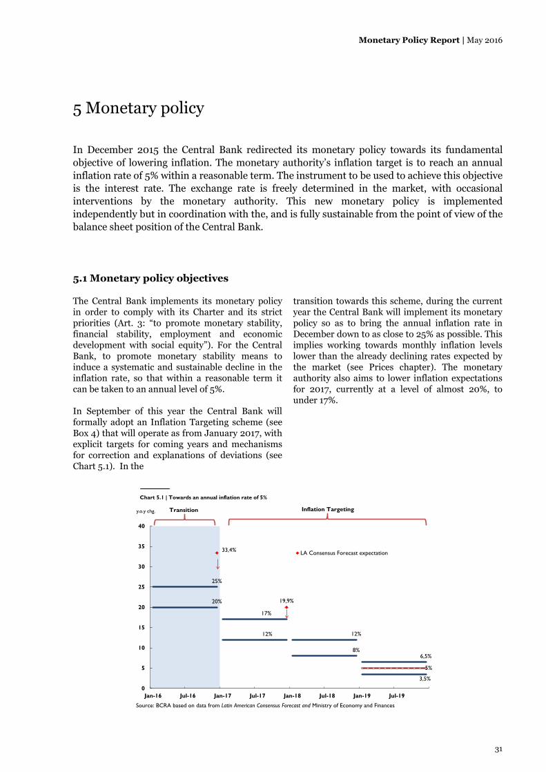
Monetary Policy Report | May 2016
31
5 Monetary policy In December 2015 the Central Bank redirected its monetary policy towards its fundamental objective of lowering inflation. The monetary authority’s inflation target is to reach an annual inflation rate of 5% within a reasonable term. The instrument to be used to achieve this objective is the interest rate. The exchange rate is freely determined in the market, with occasional interventions by the monetary authority. This new monetary policy is implemented independently but in coordination with the, and is fully sustainable from the point of view of the balance sheet position of the Central Bank. 5.1 Monetary policy objectives
The Central Bank implements its monetary policy in order to comply with its Charter and its strict priorities (Art. 3: “to promote monetary stability, financial stability, employment and economic development with social equity”). For the Central Bank, to promote monetary stability means to induce a systematic and sustainable decline in the inflation rate, so that within a reasonable term it can be taken to an annual level of 5%. In September of this year the Central Bank will formally adopt an Inflation Targeting scheme (see Box 4) that will operate as from January 2017, with explicit targets for coming years and mechanisms for correction and explanations of deviations (see Chart 5.1). In the
transition towards this scheme, during the current year the Central Bank will implement its monetary policy so as to bring the annual inflation rate in December down to as close to 25% as possible. This implies working towards monthly inflation levels lower than the already declining rates expected by the market (see Prices chapter). The monetary authority also aims to lower inflation expectations for 2017, currently at a level of almost 20%, to under 17%.
Chart 5.1 | Towards an annual inflation rate of 5%
25%
20%
17%
12% 12%
8%6,5%
3,5%
5%
33,4%
19,9%
0
5
10
15
20
25
30
35
40
Jan-16 Jul-16 Jan-17 Jul-17 Jan-18 Jul-18 Jan-19 Jul-19
y.o.y chg.
LA Consensus Forecast expectation
Source: BCRA based on data from Latin American Consensus Forecast and Ministry of Economy and Finances
Transition Inflation Targeting

CENTRAL BANK OF ARGENTINA
32
5.2 Interest rate as a tool As from the end of February, the Central Bank has adopted the interest rate as the main instrument of its monetary policy. In this initial stage it has defined as its monetary policy rate the rate resulting from the 35-day peso LEBAC auction, at the same time as setting a corridor for its repos and reverse repos consistent with the policy rate. The main advantage of using the interest rate as a monetary policy instrument is that it should not necessarily be altered when there are changes in the demand for money. In addition, it makes it possible to demonstrate the Central Bank’s position with respect to inflation in a more transparent manner; in the current context, it can set a real rate of interest that is sufficiently positive in comparison to expected future inflation. In addition, it offers greater predictability by encouraging a more stable yield for domestic currency assets (see Box 5).
Once the interest rate has been defined, the monetary base and aggregates increase or decrease in relation to liquidity needs, without necessarily generating inflationary or deflationary pressures. Any expansion in the amount of money not validated by an increase in demand is automatically absorbed by bills, notes, public bonds or reverse repos. As from the end of February, when the Central Bank adopted the 35-day LEBAC as the principal tool of its monetary policy, it set that rate first at 37% and later at 38%. In addition, it began to play a more active role in the secondary LEBAC market (see Chart 5.2). At the beginning of May, in response to lower underlying inflation in April, and to limit any contractive bias from its monetary policy, it modified its monetary policy rate to 37.5%, its current level.
Chart 5.2 | LEBAC interest rate and amount traded by BCRA in the secondary market (35-day LEBAC)
0
1
2
3
4
5
20
25
30
35
40
45
50
15-Dec-15 04-Jan-16 24-Jan-16 13-Feb-16 04-Mar-16 24-Mar-16 13-Apr-16 03-May-16
Source: BCRA
billion $Amount traded by the BCRA in the secondary market (right scale)
Secondary market interest rate
Weekly auction interest rate
APR %
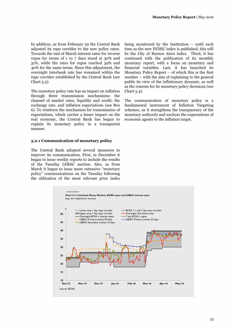
Monetary Policy Report | May 2016
33
In addition, as from February 29 the Central Bank adjusted its repo corridor to the new policy rates. Towards the end of March interest rates for reverse repos for terms of 1 to 7 days stood at 30% and 31%, while the rates for repos reached 39% and 40% for the same terms. Since this adjustment, the overnight interbank rate has remained within the repo corridor established by the Central Bank (see Chart 5.3). The monetary policy rate has an impact on inflation through three transmission mechanisms: the channel of market rates, liquidity and credit; the exchange rate, and inflation expectations (see Box 6). To reinforce the mechanism for transmission of expectations, which carries a lesser impact on the real economy, the Central Bank has begun to explain its monetary policy in a transparent manner.
5.2.1 Communication of monetary policy The Central Bank adopted several measures to improve its communication. First, in December it began to issue weekly reports to include the results of the Tuesday LEBAC auction. Also, as from March it began to issue more extensive “monetary policy” communications on the Tuesday following the ublication of the most relevant price index
being monitored by the Institution – until such time as the new INDEC index is published, this will be the City of Buenos Aires index. Third, it has continued with the publication of its monthly monetary report, with a focus on monetary and financial variables. Last, it has launched its Monetary Policy Report – of which this is the first number – with the aim of explaining to the general public its view of the inflationary dynamic, as well as the reasons for its monetary policy decisions (see Chart 5.4). The communication of monetary policy is a fundamental instrument of Inflation Targeting schemes, as it strengthens the transparency of the monetary authority and anchors the expectations of economic agents to the inflation target.
Chart 5.3 | Interbank Money Markets, BCRA repos and LEBAC interest rates (avg. rate weighted per amount)
10
15
20
25
30
35
40
45
50
Oct-15 Nov-15 Dec-15 Jan-16 Feb-16 Mar-16 Apr-16 May-16
Lower area 1 day repo corridor BCRA´s 1 and 7 day repo corridorUpper area 7 day repo corridor Overnight Call interes rateOvernight BCRA´s reverse repos 7 day BCRA´s reposLEBAC Primary market 90 days LEBAC Primary market 35 daysLEBAC Secondary market 15 days
Source: BCRA
%

CENTRAL BANK OF ARGENTINA
34
5.3 A new exchange regime In line with its intention to adopt an Inflation Targeting scheme, the Central Bank migrated as from December to a flexible exchange rate regime. The Institution considers that a floating exchange rate will be important to decouple movements in the exchange rate from the behavior of domestic prices. Furthermore, limiting the (pass-through) transfer of movements in the nominal exchange rate to prices is crucial for the real exchange rate to fulfill its stabilizing role in the event of shocks of various types. The monetary authority has nevertheless retained the possibility of intervening occasionally in the exchange rate market to administer the profile of its balance sheet and forestall unwarranted fluctuations in the exchange rate. As from December 17, when most of the restrictions on exchange rate market operations were lifted (see section 5.5), the exchange rate has for the most part been left to float (see Chart 5.5). The Central Bank only intervened on 20 days since then, buying US$1.324 billion on 11 days (at an average of 14.25 $/US$) and selling US$1.418 billion on 9 days (at an average of 15.03 $/US$ ; see Chart 5.6).
Chart5.5 | Exchange rate and BCRA operations
8.0
9.5
11.0
12.5
14.0
15.5
17.0
-300
-150
0
150
300
450
600
02-Mar-15 12-Jun-15 18-Sep-15 31-Dec-15 12-Apr-16
$/US$billion US$
BCRA purchasesBCRA salesOfficial exchange rate (right axis)Alternative exchange rate* (right axis)
*Arbitrage of the same bond traded in the local and foreign marketSource: BCRA
Gap+50% +45%
Chart 5.6 | BCRA operations in the Exchange rate market
Average exchange rate of sales:15,03
Average exchange rate of purchases:
14,25
9.0
10.0
11.0
12.0
13.0
14.0
15.0
16.0
-450
-300
-150
0
150
300
450
600
17-Dec-15 18-Jan-16 17-Feb-16 16-Mar-16 15-Apr-16
billion US$
BCRA purchases
BCRA sales
Exchange rate (right axis)
Source: BCRA
$/US$
Chart 5.4 | Monetary policy communication
Monetary Policy Report Monthly Monetary Report Report to the National CongressWednesday, June 15
Central Bank Bills Auction SpeechEvery Tuesday
Monetary Policy Speech
Friday, December 30
MAY 2016 JUNE 2016 JULY 2016 AUGUST 2016
SEPTEMBER 2016 OCTOBER 2016 NOVEMBER 2016 DECEMBER 2016SUN MON TUE WED THU FRI SAT SUN MON TUE WED THU FRI SAT SUN MON TUE WED THU FRI SAT SUN MON TUE WED THU FRI SAT
SUN MON TUE WED THU FRI SAT SUN MON TUE WED THU FRI SAT SUN MON TUE WED THU FRI SAT SUN MON TUE WED THU FRI SAT
Targets and programs for the
development of monetary, exchange
rate, �nancial and credit policies
for 2016
Monday, May 9Monday, July 18Tuesday, October 18
Friday, May 6Tuesday, June 7�ursday, July 7Friday, August 5Wednesday, September 7 Friday, October 7Monday, 7 NovemberWednesday, December 7
Tuesday a�er the publication of the In�ation index

Monetary Policy Report | May 2016
35
5.4 Monetary and fiscal coordination and the Central Bank balance sheet The Central Bank has agreed on a cap on the transfer of resources to the Treasury for 2016 equivalent to $160 billion. The fact of having clarified and placed a limit on the amount of transfers to the Treasury, together with not having committed to any given exchange rate, has given the monetary authority the necessary flexibility and predictability for it to be able to focus on its aim of lowering inflation. The amount of transfers agreed for 2016 in no way compromises the aim of the institution or its balance sheet (see Box 7).
5.5 The path to inflation targeting The path towards the adoption of an Inflation Targeting scheme, planned for September, began with an initial stage in which the Central Bank worked to correct the imbalances that existed in the economy in 2015 and absorb excess liquidity (see Chart 5.7).
In effect, until December 2015 the exchange rate market was affected by a series of restrictions on the purchase of foreign currency (which became known as the “exchange clamp”), with a gap of over 50% between the official exchange rate and the implicit rate in financial assets and heavy intervention by the monetary authority to support the official rate in a context of high uncertainty. In addition, monetary policy was subordinated to fiscal objectives (see Chart 5.8) as well as exchange rate objectives, implying a sharp rate of increase in monetary aggregates. As part of the preparation for the switch to an Inflation Targeting scheme with a floating exchange rate, the Central Bank has taken a series of measures to normalize the operation of the exchange rate and monetary markets.
Chart 5.7 | Towards an Inflation Targeting regime

CENTRAL BANK OF ARGENTINA
36
5.5.1 Exit from the “clamp” On December 17 the monetary authority lifted restrictions on the flow of current transactions and the purchase of foreign currency for forming of external assets for up to US$2 million per month for natural or legal persons, a limit that was raised at the beginning of May to US$5 million per month (although the obligation to settle export proceeds on the exchange market was maintained). The result of this measure was the almost complete unifying of the exchange market at an initial level of around $14 per US dollar.
5.5.2. Strengthening of the Central Bank balance sheet Within the framework of this liberalization, the Central Bank took various measures to strengthen its balance sheet, improving its liquidity in US dollars. First, it agreed the partial conversion into dollars of the yuans corresponding to the currency swap agreed between the Central Bank and the Central Bank of the People’s Republic of China. Second, it carried out the exchange of 3 Non-Transferrable National Treasury Bills for a total of US$16 billion for new issues of BONAR 2022, BONAR 2025 and BONAR 2027, assets of much greater liquidity. Indeed, at the end of January the Central Bank used these bonds to enter into a repo agreement in US dollars for US$5 billion with banks abroad for a term of approximately 1 year (see Chart 5.9).
5.5.3. Elimination of financial market restrictions To normalize the operation of the financial system, a crucial channel for the transmission of monetary policy, the Central Bank scrapped the limits on loan and deposit interest, leaving these transactions to be freely agreed between financial institutions and their customers. As a consequence of this measure and the greater confidence inspired in the peso, private sector deposits, which had been falling sharply in the weeks prior to the unifying of the exchange market, showed strong growth as from the second half of December. This trend would have been even greater had it not been for a drop in time deposits for amounts of over $1 million, probably due to their having been attracted by the yield on Central Bank instruments (see section 5.2).
5.5.4 Absorption of excess liquidity
Since December 2015 the Central Bank has assumed responsibility for the absorption of excess liquidity generated by strong monetary expansion in the past. In addition, it has had to neutralize the expansive monetary effect of the over $52 billion in losses linked to futures transactions entered into in 2015 (see Chart 5.10).
Chart 5.8 | Transfer of profits and financing demands to the Treasury
160
1.6
0.5
5.0
0.5
0.9
1.2
3.73.5
4.3
4.7
6.1
5.2
2.5
0
1
2
3
4
5
6
7
0
50
100
150
200
250
300
350
2004 2005 2006 2007 2008 2009 2010 2011 2012 2013 2014 2015 2016f
% GDPbillion $
Use of international reserves
Temporary advances+transfer of profits
Total as % of GDP (right scale)
Source: BCRA f: forecast
Chart 5.9 | BCRA International reserves
0
5
10
15
20
25
30
35
40
0
5
10
15
20
25
30
35
40
7-Dec-15 23-Dec-15 31-Jan-16 30-Apr-16
%billion US$
Rest of reserves China swap (in yuans)China swap (in dollars) Reverse repo with entitiesInternational reserves / asset (right axis)
Source: BCRA
Chart 5.10 | Monetary Base Explanatory factors (contribution per factor to the y.o.y change)
40.527.1
-80
-40
0
40
80
120
2004 2006 2008 2010 2012 2014 2016*
p.p.
OtherForeign exchange purchasesPublic SectorLEBAC-NOBAC and ReposMB
*Accumulated figure corresponding to the last 12 months up to April 2016. The item “Other” includes the cancelation of rediscount or the operations related to the bicentenary credit line, purchase/sale of government securities, and gain/loss for exchange rate futures, among others. The y.o.y change of the MB is influenced by changes in reserve requirements, which in 2006 registered an increase, and since 2010 decreases.Source: BCRA.
3.4
-6.4
-16
-8
0
8
16
4m-15 4m-16
p.p.
Exchange rate
futures effect
12 -month changeFour-month change

Monetary Policy Report | May 2016
37
Specifically, the monetary authority placed Bills on the primary market, made sales in the secondary market, and used the repo window, with a total contractive effect of $108 billion in the first four months of the year. To sharpen its monetary policy tools, it introduced a wider range of rates and terms for its securities, re-launching LEBAC bills in pesos adjusted by the exchange rate and including securities for shorter terms, as from 35 days. At the same time, it expanded the universe of potential holders, once again allowing them to be acquired by non-residents. It also changed the auction mechanisms, eliminating the predetermined interest rates segment. As a result of these actions, the year-on-year rate of growth in the monetary base fell by over 13.4 percentage points (p.p.) compared to that recorded in December, reaching 27.1% y.o.y. in April after a year-on-year low of 25% in February38 (see Chart 5.11). Sharp reductions in the growth rate were also recorded for the rest of the monetary aggregates. The broadest private sector aggregate in pesos (private M339) posted a year-on-year variation of 29.3% in April, which was 10.9 p.p. down on that for the last month of 2015, while private sector
38 The monetary base posted a temporary acceleration in its growth in March, mainly for regulatory reasons. In the context of a quarterly Minimum Cash requirement (in effect between December and February), and facing the imminent unifying of the exchange market, financial institutions recorded an unusual-ly high level of cash reserve requirement compliance in Decem-ber, which they offset with lower compliance in the two subse-quent months, particularly in February. With the start of the new calculation period in March, financial institutions were obliged to rebuild their banking reserves. 39 Private M3 is made up of cash in the hands of the public, settlement checks in pesos and deposits by the private and public non-financial sectors in pesos.
means of payment (private M2 40) lowered their growth rate by over 11.2 p.p. compared with the end of 2015, showing a year-on-year change of 25.5% (see Chart 5.12).
40 Private M2 is made up of cash in the hands of the public, settlement checks in pesos and private sector sight deposits.
Chart 5.11 | Monetary Base
-10
0
10
20
30
40
50
Apr-08 Apr-09 Apr-10 Apr-11 Apr-12 Apr-13 Apr-14 Apr-15 Apr-16
y.o.y chg.
Monetary baseMoney held by the publicBank reserves
Source: BCRA
Chart 5.12 | Monetary Aggregates (monthly avg. changes)
-20
-10
0
10
20
30
40
50
-4
-2
0
2
4
6
8
10
Apr-08 Apr-09 Apr-10 Apr-11 Apr-12 Apr-13 Apr-14 Apr-15 Apr-16
%%
Private M2 monthly change
Private M3 y.o.y change (right scale)
Private M2 y.o.y change (right scale)
Note: M3 includes money held by the public and total deposits in pesos.
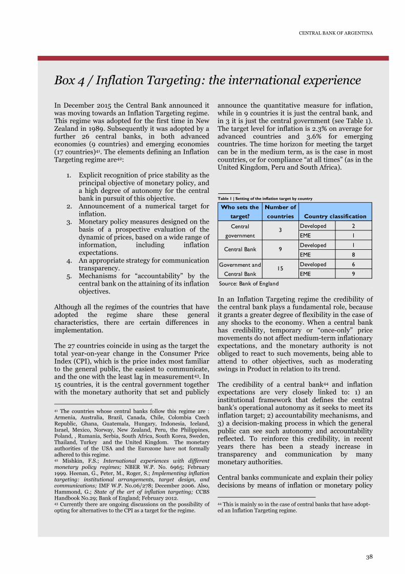
CENTRAL BANK OF ARGENTINA
38
Box 4 / Inflation Targeting: the international experience In December 2015 the Central Bank announced it was moving towards an Inflation Targeting regime. This regime was adopted for the first time in New Zealand in 1989. Subsequently it was adopted by a further 26 central banks, in both advanced economies (9 countries) and emerging economies (17 countries)41. The elements defining an Inflation Targeting regime are42:
1. Explicit recognition of price stability as the principal objective of monetary policy, and a high degree of autonomy for the central bank in pursuit of this objective.
2. Announcement of a numerical target for inflation.
3. Monetary policy measures designed on the basis of a prospective evaluation of the dynamic of prices, based on a wide range of information, including inflation expectations.
4. An appropriate strategy for communication transparency.
5. Mechanisms for “accountability” by the central bank on the attaining of its inflation objectives.
Although all the regimes of the countries that have adopted the regime share these general characteristics, there are certain differences in implementation. The 27 countries coincide in using as the target the total year-on-year change in the Consumer Price Index (CPI), which is the price index most familiar to the general public, the easiest to communicate, and the one with the least lag in measurement43. In 15 countries, it is the central government together with the monetary authority that set and publicly
41 The countries whose central banks follow this regime are : Armenia, Australia, Brazil, Canada, Chile, Colombia Czech Republic, Ghana, Guatemala, Hungary, Indonesia, Iceland, Israel, Mexico, Norway, New Zealand, Peru, the Philippines, Poland, , Rumania, Serbia, South Africa, South Korea, Sweden, Thailand, Turkey and the United Kingdom. The monetary authorities of the USA and the Eurozone have not formally adhered to this regime. 42 Mishkin, F.S.; International experiences with different monetary policy regimes; NBER W.P. No. 6965; February 1999. Heenan, G., Peter, M., Roger, S.; Implementing inflation targeting: institutional arrangements, target design, and communications; IMF W.P. No.06/278; December 2006. Also, Hammond, G.; State of the art of inflation targeting; CCBS Handbook No.29; Bank of England; February 2012. 43 Currently there are ongoing discussions on the possibility of opting for alternatives to the CPI as a target for the regime.
announce the quantitative measure for inflation, while in 9 countries it is just the central bank, and in 3 it is just the central government (see Table 1). The target level for inflation is 2.3% on average for advanced countries and 3.6% for emerging countries. The time horizon for meeting the target can be in the medium term, as is the case in most countries, or for compliance “at all times” (as in the United Kingdom, Peru and South Africa). In an Inflation Targeting regime the credibility of the central bank plays a fundamental role, because it grants a greater degree of flexibility in the case of any shocks to the economy. When a central bank has credibility, temporary or “once-only” price movements do not affect medium-term inflationary expectations, and the monetary authority is not obliged to react to such movements, being able to attend to other objectives, such as moderating swings in Product in relation to its trend. The credibility of a central bank44 and inflation expectations are very closely linked to: 1) an institutional framework that defines the central bank’s operational autonomy as it seeks to meet its inflation target; 2) accountability mechanisms, and 3) a decision-making process in which the general public can see such autonomy and accountability reflected. To reinforce this credibility, in recent years there has been a steady increase in transparency and communication by many monetary authorities. Central banks communicate and explain their policy decisions by means of inflation or monetary policy
44 This is mainly so in the case of central banks that have adopt-ed an Inflation Targeting regime.
Table 1 | Setting of the inflation target by country Who sets the
target?Number of countries
Developed 2
EME 1
Developed 1
EME 8
Developed 6
EME 9
Source: Bank of England
Country classification
Central
government
Central Bank
Government and
Central Bank
3
9
15

Monetary Policy Report | May 2016
39
reports (usually quarterly), communiqués and/or public announcements following the meetings at which they take their decisions, the minutes of such meetings, open letters when targets have failed to be met, and appearances by officials before the legislative branch (see Table 2)45. For the adoption of an Inflation Targeting regime to be successful, there are certain pre-requisites: 1) the technical capability of the central bank in its implementation; 2) absence of fiscal dominance; 3) a sound financial system, together with 4) an institutional framework that supports and encourages compliance with the inflation target46. The principal policy instrument used by central banks with Inflation Targeting regimes is the interest rate, which may be a market rate or one from an operation of the central bank itself. One of the advantages of this instrument is that it makes it possible to indicate the policy bias and the position of the monetary authority in the face of inflation in a clear and transparent manner, which contributes to transparency in communication. In addition, so as to provide greater transparency on the operation of the regime, many central banks schematically explain their channels for transmission through which their monetary policy operates (see section 6) and the lags with which it is operating. The experience of those countries that have imple-mented such regimes has largely been successful.
45 Heenan et al, 2006. 46 Does inflation targeting work in emerging markets?; World Economic Outlook (WEO); Chapter 4; IMF; September 2005.
In general, in the countries that have adopted them empirical literature documents lower inflation and volatility in prices, and also, to a lesser extent, low-er volatility in growth (see Charts 1 and 2).
Table 2 | Tools for communication in Inflation Targeting schemes
Number of countries
Developed 2
EME 5
Developed 7
EME 13
Number of countries
Developed 3
EME 5
Developed 0
EME 2
Developed 6
EME 11
Number of countries
Developed 6
EME 12
Developed 3
EME 6
If the target is not fulfilled Country classification
Open letter
No open letter
7
20
17
Announcement of policydecision
Press release
Press conference
Both
Source: Bank of England
Country classification
8
2
Publication of minutes Country classification
18
9
Yes
No
Chart 1 | Inflation Rates (before and after the adoption of Inflation Targeting)
Arm
Aus
Bra
Can
Chl
Col
Gha
GtmHun
Isl Idn
IsrKor Mex
NzlNor
PerPhl
PolCze
Rum
SrbZaf
Swe
Tha
Tur
Gbr
0
5
10
15
20
25
0 5 10 15 20 25
%
%
Note: Average of the inflation rate measured as the y.o.y. change of the CPI (December of each year). It was taken into account five years before the adoption of the IT regime (whether data were available and with the exception of Brazil). In the case of the inflation rate after adopting the regime, it were taken into account all the years available up to 2014.Source: BCRA based on IMF.
Inflation Rate after adopting the IT regime
Inflation Rate before adopting the IT regime
Chart 2 | Volatility of inflation (before and after the adoption of Inflation Targeting)
ArmAus
Bra
CanChl Col
Gha
GtmHun
Isl
IdnIsr
Kor MexNzlNor
Per Phl
PolCze Rum
Srb
Zaf
SweThl
Gbr0
3
6
9
12
15
0 3 6 9 12 15
Inflation Rate volatility after adopting the IT
regime
Inflation Rate volatility before adopting the IT regime
Note: Standard deviation of the average of the inflation rate measured as the y.o.y. change of the CPI (December of each year). It was taken into account five years before the adoption of the IT regime (whether data were available and with the exception of Brazil). In the case of the inflation rate after adopting the regime, it were taken into account all the years available up to 2014. In the case of Turkey the volatility before the adoption of the regime was above 20 p.p. and after it reduced below 2 p.p.Source: BCRA based on IMF.
p.p.
p.p.

CENTRAL BANK OF ARGENTINA
40
Box 5 / Savings and financial investments under a flexible exchange rate regime In December 2015 the Central Bank centered its economic policy on achieving price stability, focusing on the level of inflation as the guide for its monetary policy, letting the exchange rate float. Under the current flexible exchange rate regime, the monetary authority can intervene in the exchange market in certain circumstances to manage the profile of its balance sheet and prevent unjustified fluctuations, but it does not commit to a given level for the exchange rate. Its commitment is to preserve the stability of local currency, that is to say, to achieve a reduction in inflation. Table 1 shows the development of monthly yield, except for the period between 17 and 31 December, of two savings options commonly favored by Argentine savers: the holding of dollars in cash and pesos in time deposits. Included in the comparison is a hypothetical possibility of making a deposit in Housing Units (UVI), an instrument created by the Central Bank recently to encourage long-term saving. The table shows that the yield on savings in dollars or time deposits was similar during the comparison period. However, the yield in pesos of the saving in dollars alternative showed far greater volatility (see Chart 1). In this period the option of a deposit in UVI would also have been very profitable for a saver.
These behaviors illustrate a characteristic feature of flexible exchange rate regimes: savings and financial investments in foreign currency may sometimes show a higher yield, and sometimes a lower yield, but will always show greater volatility compared with investments in pesos, given the fluctuations in the exchange rate.
Table1 | Yield on savings alternatives*
PeriodDeposits in
pesosUS$ in cash
UVI (spread 0)
March 2.07% -6.67% 4.04%
February 2.01% 12.10% 3.74%
January 1.84% 6.84% 2.20%
Dec-17-15 to Dec-31-15 2.66% -9.33% 2.15%
Dec-17-15 to Mar-31-16 7.53% 6.14% 11.56%
Average yield 2.15% 0.73% 3.03%Standard deviation 0.31% 8.98% 0.87%
Source: BCRA
*Rates accrued by business or calendar days (as appropiate). Monthly rates are reported for december. For the Dec-17-
15 to Mar-31-16 period, december yields were not monthly converted.
Chart 1 | Yield and volatility of savings alternatives
7.5
0.3
6.1
9.0
11.6
0.9
0
2
4
6
8
10
12
14
Yield Dec-17-15 to Mar-31-16 Standard deviation
%
Deposits in pesos US$ in cash UVI (spread 0)
Source: BCRA

Monetary Policy Report | May 2016
41
Box 6 / Interest rates and inflation Use of an interest rate as an instrument of monetary policy is the norm in the 27 countries that have adopted Inflation Targeting mechanisms (see Box 4). It is a novelty in Argentina, however. How does a monetary policy interest rate affect inflation? Diagram 1 helps to visualize and understand the principal mechanisms by means of which rate decisions impact on prices. In first place, the monetary policy interest rate impacts directly on market interest rates, liquidity and credit. These variables in turn impact on aggregate spending, and the latter impacts on inflation. This is the first transmission mechanism. Second, the interest rate influences the rate of exchange, and the latter has a certain impact on aggregate spending, but in particular it impacts directly on many prices, and specifically on tradable goods. This impact is reflected in the transmission coefficient (see Box 3). This is the second transmission mechanism. Third, the rate decision, accompanied by communication from the central bank, influences inflation expectations. If agents in the economy perceive that the monetary authority is using its instruments to bring down inflation, they incorporate this information to their price and wage-forming processes even before effects are seen from the other mechanisms mentioned. This is the third transmission mechanism. The relative size and importance of each of these mechanisms differs among economies and even in the same country at different moments, depending on its structural characteristics – such as the depth of credit or the openness of the economy – as well
as its institutional characteristics. In Argentina, although the Central Bank is studying the strengths and the lags with which each of these mechanisms exert an impact, it is difficult to determine their precise dimension because the interest rate has never been used as an instrument of monetary policy. Nevertheless, there are signs of the probable relative importance of these channels in comparison with other countries. First, there are indications that the transmission mechanism involving aggregate spending is limited in its impact compared with other countries. This is because Argentina has a financial system that is not highly developed, with a very low credit to GDP ratio (Chart 1), although the interest rate could affect the opportunity cost of spending regardless of the size of lending. Second, the transmission mechanism that involves the exchange rate seems to be comparable to that of other countries (see Box 3). Last, as the use of the interest rate as an instrument is very recent, it is likely that the transmission mechanism that affects expectations is still in its infancy. Nevertheless, the limited transfer to prices of the huge corrections to relative prices in the first months of 2016 suggests that it is not inconsidera-ble. This transmission mechanism is the most interest-ing of the three because it has the least impact on the real economy. When it takes effect, monetary policy serves as a device for coordination, so that
Diagram 1 | Transmission mechanisms of the monetary policy rate
Monetarypolicy
interest rate
Inflation rateInflationexpectations
Exchange rate Aggregate spending
Market interestrates, liquidity and
credit
Chart 1 | Credit to the private sector
13,3
0
20
40
60
80
100
120
140
160
180
Spai
n
Swit
zerl
and
Por
tuga
l
Aus
tral
ia
UK
Ger
man
y
Japa
n
US
Chi
na
Tha
iland
Tur
key
Sout
h A
fric
a
Rus
ia
Rum
ania
Chi
le
Bra
zil
Col
ombi
a
Bol
ivia
Ven
ezue
la
Per
u
Uru
guay
Mex
ico
Arg
enti
na
% of GDP
Note: Data up to 2015, except Argentina up to february 2016, (estimated data)Source: BCRA from IMF and Central Banks data
Advanced (avg.138%)
Other emerging(avg.86%)
Latin America (avg.41%)

CENTRAL BANK OF ARGENTINA
42
variations in relative prices occurring naturally in the economy materialize with smaller nominal variations. In the absence of fiscal dominance or other elements conditioning monetary policy, there is nothing to prevent it from fulfilling its coordinat-ing role to lower inflation. That is why the Central Bank seeks to strengthen the effect of its monetary policy on expectations by means of increased and improved communication with the general public.

Monetary Policy Report| May 2016
43
6.0 5.2
-4.6 -4.8
-300
-225
-150
-75
0
75
150
225
300
-8
-6
-4
-2
0
2
4
6
8
2004 2005 2006 2007 2008 2009 2010 2011 2012 2013 2014 2015
% of GDP
Using free reserves (right axis)Profits (right axis)Net grant temporary advances (right axis)BCRA transfers to the National TreasuryPrimary balance of National Treasury without income
* Transfers by special allocations of Special Drawing Rights (SDR) of the IMF in 2009 and 2010 are not considered (by $ 9,575,000 million and $ 777 million, respectively).Source: BCRA from Ministery of Treasury and Public Finance and INDEC data
billion $
the national treasury without Central Bank
Box 7 / Monetary policy interaction with the Treasury In a context of growing fiscal imbalances and voluntary credit market rationing, and through the use of various mechanisms, in recent years the Central Bank became one of the main sources of financing for the significant requirements for funds by the Treasury. One of the consequences of this situation was that the emission designed to meet this constant demand for resources was transformed into an independent monetary base creation factor of the first order. This caused a marked monetary imbalance that was the root cause of the acceleration in inflation experienced by the Argentine economy in the past decade. In such conditions, the country experienced the development of a typical situation of fiscal dominance of its monetary policy. As has been analyzed in theoretical and empirical literature48, in such systems the decisions of the monetary authority lose autonomy and give way to those of fiscal policy. In this regard, a basic requirement for ensuring a steady decline in the rate of inflation will be to escape from the fiscal dominance that has been inherited.
48 Systems for coordination —either implicit or explicit — between monetary and fiscal policies and the resulting interaction between them has been the subject of intense scrutiny by theoretical and empirical literature. A at a theoretical level Sargent and Wallace (1981). “Some unpleasant monetarist arithmetic”; Federal Reserve Bank of Minneapolis; has become a classic reference, but others provide a useful source for consultation, such as Leeper, E. M. (1991). “Equilibria under ‘active’ and ‘passive’ monetary and fiscal policies”; Journal of Monetary Economics, 27(1), 129-147. What these writings show is that in fiscal dominance situations (that is to say, in circumstances in which structural fiscal underfunding imposes on the central bank to continually monetize budgetary imbalances), the residual recourse to seigniorage in the final instance prevents monetary policy from exercising nominal control of the system. When that happens, monetary policy becomes “passive” and the central bank authorities find themselves unable to anchor private sector expectations (which it turn negatively affects the public’s demand for money). In such circumstances, if there are limits on the amount of public debt the market is prepared to absorb, monetary policy becomes incapable of having a permanent impact on the rate of inflation in the economy( in fact explained by the present value of the fiscal need for resources, determined “exogenously” for the monetary authorities). In such instances there can even be “paradoxical” results, such as when a current monetary restriction effectively leads to higher prices than those corresponding to a lax monetary policy (see Drazen (1985). “Tight Money and Inflation: Further Results”, Journal of Monetary Economics, 15, pp. 113-20). Empirical study of numerous experiences —in both developing countries and advanced economies – in which the passive monetization of fiscal imbalances has given rise to the generation of episodes of high inflation and hyperinflation, is a vivid illustration of these phenomena. For a detailed study of the working of these mechanisms in the local case, see Heymann and Leijonhufvud (1995). “High Inflation: The Arne Ryde Memorial Lectures”; Clarendon Press, Oxford, 1995.
This will allow monetary policy to gradually recover a degree of freedom to anchor expectations and influence the nominal development of the economy in the direction of a persistent decline in inflation levels. The deterioration in public finances and the restriction on access to external financing in recent years led to growing dependence on the various mechanisms for transferring Central Bank resources to the Treasury (see Chart 1). In 2015 such funding totaled over 5 percentage points of GDP, covering not only the entire primary deficit but also a substantial part of the public sector’s capital and interest maturities. While the placing of Non-Transferrable Bills as a counterpart to the use of international reserves represented around 2% of GDP during that year, recourse to financing with a domestic monetary impact (temporary advances under Article 20 of the Charter and the transfer of profits) was equivalent to over 3% of GDP.
One consequence of this situation was that in recent years fiscal monetary financing became the main factor behind monetary base growth (see Chart 2). There it can be seen that if before 2009 the public sector was a factor that on a net basis contributed in a contractive manner to the evolution of the monetary base, that situation altered drastically as from 2010, when the monetization of fiscal imbalances came to represent more than the total amount of the net growth of high power money. Despite the fact that —with a differing intensity depending on the stage— the Central Bank sought to sterilize part of this growth in the money supply by placing Bills to adjust it to the evolution of the demand for

CENTRAL BANK OF ARGENTINA
44
monetary base, the high rate of growth imposed by the growing need for fiscal financing (and a weak demand for domestic financial assets in a high inflation context) led to a marked imbalance in the money market. This imbalance was at the base of a trend towards a systematic rise in the rate of inflation being recorded.
The intention of the Central Bank and the economic authorities is to reverse this dynamic, as a basic prerequisite for a gradual but steady decline in inflation. As part of the gradual process for fiscal reorganization and the normalizing of access to external voluntary credit markets that is currently taking place, it has been agreed by the monetary authorities and the Executive Branch to make a start on significantly reducing the financing provide by the Central Bank to the Treasury. This will still mean the commitment of a certain volume of monetary resources to finance the fiscal deficit during a period of transition. It has been agreed that during the current year the Central Bank will make transfers to the Treasury of net temporary advances and profits for a total of $160 billion (2.1% of GDP), at the rate of some $40 billion per quarter. In real terms, this represents a reduction in the order of 20% compared with the amount transferred to the Treasury last year as net temporary advances and profits. During the last week of April, when presenting the financial program following the agreement reached in the dispute with foreign creditors, the Minster of the Treasury and Public Finances formally and publicly announced that the financing that the Treasury expected to receive from the Central Bank was as indicated above. The Executive has committed to a reduction in this figure in coming years. The shared objective is to exit in a definitive manner from the fiscal dominance structure that has
seriously conditioned monetary policy actions in recent years and has led to the high inflation environment for which the current functioning of the Argentine economy is noted. Unlike the situation in previous years, the figure for Treasury financing committed to by the Central Bank for 2016 is entirely consistent with the dynamic envisaged for the decline in the rate of inflation49. The Central Bank estimates that the increase in monetary base demand will exceed the remaining transfers to the Treasury for 2016 ($120 billion) by between $53 billion and $95 billion (see Chart 3). This can be determined from the projection for demand of real M2 balances by the private sector – which is expected to increase in nominal terms at the end of the current year by between 16.4% y.o.y. and 22.8% y.o.y. with a central forecast of 19.6% y.o.y.— and the forecasts for the evolution of the monetary multiplier. In these conditions, the demand for monetary base by the public and financial institutions will enable the absorption of the total amount of monetary emission foreseen for the financing of the Treasury, without it giving rise to subsequent inflationary pressures. The existence of this potential excess monetary base demand will gradually provide the Central Bank with a degree of freedom to manage its monetary policy. Depending on the circumstances, the monetary authority will be able to meet surplus demand for primary liquidity by opting between reducing the stock of LEBAC and/or increasing its
49 See the 2016 monetary presentation program.. http://www.bcra.gov.ar/Pdfs/Prensa_comunicacion/ PresentacionPoliticasMonetarias2016.pdf
Chart 3 | Nominal monetary base demand and effect of Central Bank transfers to the Treasury (standard deviation bands)
Chart 2 | Factors making up the monetary base Chart 1 | Primary result for
-60
-40
-20
0
20
40
60
80
100
2004 2005 2006 2007 2008 2009 2010 2011 2012 2013 2014 2015
contribution to the y.o.y. % chg. Others
Foreing exchanges purchases
Public Sector
LEBAC-NOBAC and Repos
MB
*Accumulated figure corresponding to the last 12 months up to April 2016. The item “Other” includes the cancelation of rediscount or the operations related to the bicentenary credit line, purchase/sale of government securities, and gain/loss for exchange rate futures, among others. The y.o.y change of the MB is influenced by changes in reserve requirements.Source: BCRA.
587
781
587
760
587
802
587
707
500
550
600
650
700
750
800
850
Sep-15 Dec-15 Mar-16 Jun-16p Sep-16p Dic-16p
billion $
MB demand
Dynamic of the money supply associated with transfers to Treasury
Source: BCRA p:proyected

Monetary Policy Report | May 2016
45
holding of foreign reserves. If it were to opt for the former of these two courses of action, the stock of LEBAC could reverse its upward dynamic, going from an average of $427 billion in March to a projected level by December of between $415 billion and $463 billion (with a central forecast of $439 billion). On the contrary, if the purchase of international reserves were to be favored, the stock of liquid assets held by the Central Bank could increase by between US$4 billion and US$6.2 billion. In the latter case, contingent on the projected base macroeconomic scenario, it is estimated that the stock of LEBAC would reach a level of around $519 billion in average balances in the final month of the year. It should be noted that in either of the possible policy courses, LEBAC stocks should show a declining dynamic as a proportion of the monetary base (see Chart 4). That is because —as has been announced in the weekly communiqués accompanying the LEBAC auctions and at the presentation of the monetary program for the year in progress – as monthly inflation levels go declining in line with the forecasts of this monetary authority, the Central Bank estimates that it will be in a position to reduce the high nominal interest rates currently in force over coming months. In particular, and in so far as a very significant portion of its sterilization instruments are concentrated at present on the shortest terms (the average life of the stock is currently around 44 days), any reduction in nominal policy rates will be rapidly translated into a reduction in the associated interest burden. In line with the gradual overcoming of the fiscal dominance situation that has been inherited, the expected evolution of the stock of LEBAC will reflect a composition of Central Bank liabilities that is compatible with increasing margins for maneuver, so that monetary policy can regain its ability to ensure an environment of nominal stability.
Chart 4 | LEBAC stocks
56.2
66.4
53.1
72.8
59.2
50
55
60
65
70
75
80
Jan-16 Mar-16 May-16p Jul-16p Sep-16p Nov-16p
% of MB
Policy option: cancellation LEBACs
Policiy option: purchase of reserves
Source: BCRA p: proyected

CENTRAL BANK OF ARGENTINA
46
Abbreviations and acronyms
€: Euro Acum.: Acumulado ADEFA: Asociación de Fábricas de Automotores de Argentina ADIMRA: Asociación de Industriales metalúrgi-cos de la República Argentina AFCP: Asociación de Fabricantes de Cemento Portland AFIP: Administración Federal de Ingresos Públi-cos AHORA 12: Programa oficial de promoción del consumo interno mediante instrumentos financie-ros AMBA: Área Metropolitana de Buenos Aires ANSeS: Administración Nacional de la Seguridad Social AT: Adelantos Transitorios AUH: Asignación Universal por Hijo para Protec-ción Social BADLAR: Buenos Aires Deposits of Large Amount Rate (tasa de interés pagada por depósitos a plazo fijo de más de un millón de pesos en el tra-mo de 30 a 35 días por el promedio de entidades bancarias) Bbl: Barriles BCB: Banco Central de Brasil BCBA: Bolsa de Comercio de Buenos Aires BCE: Banco Central Europeo BCRA: Banco Central de la República Argentina Bim: Bimestre BNDES: Banco Nacional de Desarrollo Bonac: Bono del Tesoro Nacional Bonad: Bono atado en dólares Bonar: Bono de la Nación Argentina BRIC: Brasil, Rusia, India y China BTU: British Thermal Unit CABA: Ciudad Autónoma de Buenos Aires Call: Tasa de interés promedio de las operaciones a 1 día hábil del mercado interfinanciero no garanti-zado CAME: Confederación Argentina de la Mediana Empresa CCBCRA: Cuenta Corriente del Banco Central de la República Argentina CEDIN: Certificados de Depósitos para la Inver-sión CEMBI+: Corporate Emerging Market Bond Index plus
CER: Coeficiente de Estabilización de Referencia CFI: Coparticipación Federal de Impuestos CGV: Cadenas Globales de Valor CNPHV: Censo Nacional de Población, Hogares y Vivienda CNV: Comisión Nacional de Valores Contrib.: Contribución DEG: Derecho Especial de Giro DGA: Dirección General de Aduanas DJVE: Declaraciones Juradas de Ventas al Exte-rior DPN: Deuda Pública Nacional e: Estimado EDP: Equipo Durable de Producción EFSF: European Financial Stability Facility EIA: Oficina de Información de Energía de los Estados Unidos ELA: Emergency Liquidity Assistance EMBI+: Emerging Markets Bond Index Plus EMEA: Europa emergente, Medio oriente y África EMI: Estimador Mensual Industrial ENARSA: Empresa Energía Argentina S.A. ENERGAS: Ente Nacional Regulador del Gas ENGH: Encuesta Nacional de Gasto de los Hoga-res ENRE: Ente Nacional Regulador de la Electricidad EPA: Agencia de Protección del Medio Ambiente de los Estados Unidos EPH: Encuesta Permanente de Hogares ERM: Exchange Rate Mechanism ETFs: Exchanged Traded Funds (fondos negocia-bles) excl.: Excluyendo FBC: Formación bruta de capital FCI: Fondos Comunes de Inversión Fed: Reserva Federal de los Estados Unidos FFS: Fondo Federal Solidario FGS: Fondo de Garantía de Sustentabilidad FMI: Fondo Monetario Internacional FOB: Free on Board (operaciones de compraventa que se realiza por barco) FOMC: Comité Federal de Mercado Abierto FONDEA: Fondo de Desendeudamiento Argen-tino FONDEAR: Fondo de desarrollo económico ar-gentino

Monetary Policy Report | May 2016
47
G-7: Estados Unidos, Japón, Alemania, Francia, Reino Unido, Italia, Canadá GBA: Gran Buenos Aires HOGAR: Programa de subsidios para adquirir la garrada social i.a.: Interanual IAMC: Instituto Argentino de Mercado de Capita-les ICA: Intercambio Comercial Argentino ICC: Índice del Costo de la Construcción ICDCB: Impuesto a los Créditos y Débitos en Cuentas Bancarias ICV: Índice del Costo de Vida IED: Inversión Extranjera Directa IFS: Institute of Fiscal Studies (Instituto de Estu-dios Fiscales) IGA-OJF: Índice General de Actividad de Orlando J. Ferreres ILA: Índice Líder de la Actividad INDEC: Instituto Nacional de Estadística y Censos INML: Índice de Novillos del Mercado de Liniers IOER: Interest on excess reserve balances IPMP: Índice de Precios de las Materias Primas IPC Nacional: Índice de Precios al Consumidor Nacional IPCBA: Índice de Precios al Consumidor de la Ciudad de Buenos Aires IPC GBA: Índice de Precios al Consumidor del Gran Buenos Aires IPCNu: Índice de Precios al Consumidor Nacional ur-bano IPCSL: Índice de Precios al Consumidor de San Luis IPI: Índice de Precios Implícitos IPI-FIEL: Índice de Producción Industrial de la Fundación de Investigaciones Económicas Lati-noamericanas IPIB: Índice de Precios Internos Básicos IPIM: Índice de Precios Internos al Por Mayor IPMP: Índice de Precios de las Materias Primas IPP: Índice de Precios al Productor ISAC: Índice Sintético de Actividad de la Cons-trucción ISM: Institute for supply management (índice de perspectivas los gerentes de compras en el sector manufacturero) ISSP: Indicador Sintético de Servicios Públicos ITCRB: Índice de Tipo de Cambio Real Bilateral ITCRM: Índice de Tipo de Cambio Real Multilate-ral IVA DGA: Impuesto al Valor Agregado Dirección General de Aduanas
IVA: Impuesto al Valor Agregado kg: Kilogramo LAC: Latin American Consensus Forecasts LCIP: Línea de Créditos para la Inversión Produc-tiva LEBAC: Letras del Banco Central (Argentina) LTRO: Long Term Refinancing Operation MAE: Mercado Abierto Electrónico M2: Billetes y monedas + cuasimonedas en circu-lación + cuentas corrientes en $ y cajas de ahorro en $ M3*: Billetes y monedas + cuasimonedas + depó-sitos totales en $ y US$ M3: Billetes y monedas + cuasimonedas en circu-lación + depósitos totales en $ MAGyP: Ministerio de Agricultura, Ganadería y Pesca MATBA: Mercado a Término de Buenos Aires Mbd: Millones de barriles por día MEM: Mercado Eléctrico Mayorista MERVAL: Mercado de Valores de Buenos Aires mill.: Millones Min.: Ministerio MIPyMEs: Micro, Pequeñas y Medianas Empre-sas MOA: Manufacturas de Origen Agropecuario MOI: Manufacturas de Origen Industrial MRO: Main Refinancing Operations MSCI: Morgan Stanley Capital International Index MTySS: Ministerio de Trabajo y Seguridad Social NOBAC: Notas del Banco Central (Argentina) OCDE: Organización para la Cooperación y el Desarrollo Económico OEDE: Observatorio de Empleo y Dinámica Em-presarial OFEPHI: Organización Federal de los Estados Productores de Hidrocarburos OIT: Organización internacional del trabajo OMA: Operaciones de mercado abierto ON: Obligaciones Negociables ON RRPs: Overnight Reverse Repurchase Agree-ment Operations ONU: Organización de las Naciones Unidas OPEP: Países Exportadores de Petróleo p.b.: Puntos básicos p.p.: Puntos porcentuales p: Proyectado PAMI: Obra Social para Jubilados y Pensionados PEA: Población Económicamente Activa PIB: Producto Interno Bruto PII: Posición de inversion internacional

CENTRAL BANK OF ARGENTINA
48
PIST: Punto de Ingreso al Sistema de Transporte PMI: Purchasing Managers’ Index PP: Productos primarios PROCER: Programa de Competitividad de Eco-nomías Regionales PROCREAR: Programa de Crédito Argentino PROCREAUTO: Plan oficial para financiar la compra de vehículos PROGRESAR: Programa de Respaldo a Estudian-tes de Argentina Prom. móv.: Promedio móvil Prom.: Promedio PyMEs: Pequeñas y Medianas Empresas P5+1: Consejo de Seguridad de las Naciones Uni-das (Estados Unidos, Francia, China, Rusia y Reino Unido) más Alemania R$: Real REPO: Repurchase Agreement (Operación de Recompra) RIPTE: Remuneraciones Imponibles Promedio de los Trabajadores Estables ROFEX: Mercado a Término de Rosario ROE: Registros de Operaciones de Exportación Rueda REPO: Tasa de interés promedio de las operaciones a 1 día hábil entre entidades financieras en el mercado garantizado S.A: Sociedad Anónima s.e.: Serie sin estacionalidad SAC: Sueldo Anual Complementario SEDLAC: Socio-Economic Database for Latin America and the Caribbean Seg.: Seguridad SELIC: Sistema Especial de Liquidação e Custo-dia (Tasa de referencia de Brasil) SENASA: Servicio Nacional de Sanidad y Calidad Agroalimentaria SIPA: Sistema Integrado Previsional Argentino SMVM: Salario mínimo vital y móvil SPNF: Sector Público Nacional no Financiero SSN: Superintendencia de Seguros de la Nación TCNM: Tipo de Cambio Nominal Multilateral TFF: Tasa de interés de los Fondos Federales tn.: Tonelada TN: Tesoro Nacional TNA: Tasa Nominal Anual Trim.: Trimestral / Trimestre UE: Unión Europea UOCRA: Unión Obrera de la Construcción de la República Argentina US$: Dólares Americanos
USDA: United States Department of Agriculture (Secretaría de Agricultura de EE.UU.) UTDT: Universidad Torcuato Di Tella UTEDyC: Unión de Trabajadores de Entidades Deportivas y Civiles VAD: Valor Agregado Doméstico VAE: Valor Agregado Extranjero Var.: Variación VAR: Modelo de Vectores Autorregresivos VN: Valor Nominal VNO: Valor Nominal original
Vol.: Volumen WTI: West Texas Intermediate WEO: World Economic Outlook YPF SA: Yacimientos Petrolíferos Fiscales Socie-dad Anónima ZLB: Zero Lower Band (restricción de no negati-vidad)