Monetary Policy and Business Cycles with Endogenous Entry andProduct Variety∗

Florin O. Bilbiie†

University of Oxford,Nuffield College

Fabio Ghironi‡

Boston College,EABCN, and NBER

Marc J. Melitz§

Princeton University,CEPR, and NBER

June 11, 2007

Abstract

This paper studies the role of endogenous producer entry and product creation for monetarypolicy analysis and business cycle dynamics in a general equilibrium model with imperfectprice adjustment. Optimal monetary policy stabilizes product prices, but lets the consumerprice index vary to accommodate changes in the number of available products. The free entrycondition links the price of equity (the value of products) with marginal cost and markups,and hence with inflation dynamics. No-arbitrage between bonds and equity links the expectedreturn on shares, and thus the financing of product creation, with the return on bonds, affectedby monetary policy via interest rate setting. This new channel of monetary policy transmissionthrough asset prices restores the Taylor Principle in the presence of capital accumulation (in theform of new production lines) and forward-looking interest rate setting, unlike in models withtraditional physical capital. We also study the implications of endogenous variety for the NewKeynesian Phillips curve and business cycle dynamics more generally, and we document theeffects of technology, deregulation, and monetary policy shocks, as well as the second momentproperties of our model, by means of numerical examples.JEL Codes: E31; E32; E52.Keywords: Business cycles; Monetary policy; Producer entry; Product variety.

∗For helpful comments, we thank Daron Acemoglu, Virgiliu Midrigan, Gernot Müller, Julio Rotemberg, MichaelWoodford, and participants in the Twenty-second NBER Annual Conference on Macroeconomics, the Thirty-eighthKonstanz Seminar on Monetary Theory and Policy, and a seminar at Boston College. We are grateful to MassimoGiovannini, Margarita Rubio, and Frank Virga for excellent research assistance. Remaining errors are our responsi-bility. Bilbiie thanks the NBER for hospitality as a Visiting Fellow while this paper was written. Ghironi and Melitzthank the NSF for financial support through a grant to the NBER.

†Nuffield College, New Road, Oxford, OX1 1NF, UK or florin.bilbiie@nuffield.oxford.ac.uk; URL:http://www.nuff.ox.ac.uk/Users/Bilbiie/index.htm

‡Department of Economics, Boston College, 140 Commonwealth Avenue, Chestnut Hill, MA 02467-3859, U.S.A.or Fabio.Ghironi@bc.edu. URL: http://fmwww.bc.edu/ec/Ghironi.php.

§Department of Economics, Princeton University, Fisher Hall, NJ 08544, U.S.A. or mmelitz@princeton.edu. URL:http://www.princeton.edu/~mmelitz.

1 Introduction

Since the mid 1980s, a large body of literature has developed in which monetary policy is analyzed in

microfounded, dynamic, stochastic, general equilibrium (DSGE) models of the business cycle with

monopolistic competition and nominal rigidity. The importance of this ‘New Keynesian’ literature

(summarized, for instance, by Woodford, 2003) for policymaking is evidenced by the current use

of such models by many central banks or international institutions as input for policy decisions.1

Most of this literature, however, relies on monopolistic competition merely as a vehicle to introduce

price (or wage) setting power and then assume that price (or wage) setting is not frictionless,

resulting in nominal rigidity and a role for monetary policy. The overwhelming majority of models

abstracts from producer entry mechanisms and assumes a constant number of producers. The

joint assumptions of monopolistic competition and no entry raise both theoretical and empirical

questions. First, absent either properly designed markup-offsetting subsidies or increasing returns

of appropriate degree, monopolistic competition in these models results in permanent (i.e., steady-

state) positive profits, casting doubts on the theoretical appeal of the zero-entry assumption.2

Furthermore, recent empirical evidence for the U.S. has substantiated the endogenous fluctuations

in the number of producers and the range of available goods that take place over the typical

length of a business cycle. A previous literature documented the strong procyclical behavior of net

producer entry (measured either as incorporated firms or as production establishments).3 Bernard,

Redding, and Schott (2006) document how existing U.S. manufacturing establishments devote a

substantial portion of their production to goods that they did not previously produce. For U.S.

aggregate manufacturing, the value of new goods produced represents just under 10% of annual

manufacturing output.4 Axarloglou (2003) and Broda and Weinstein (2007) directly measure the

introduction of new varieties in the U.S. economy and document a strong correlation with the

business cycle. Across a wide sample of U.S. consumer purchases, Broda and Weinstein (2007)

document that a 1% increase in aggregate sales is associated with a 0.35% increase in the sales of

1See, for instance, the IMF’s GEM model (illustrated by Laxton and Pesenti, 2003, among others) and the FederalReserve Board’s SIGMA model (illustrated by Erceg, Guerrieri, and Gust, 2005, among others).

2Rotemberg and Woodford (1995) addressed the implausibility of positive steady-state profits by assuming in-creasing returns to scale induced by fixed, per-period costs. However, under this assumption, any shock that causesprofits to fall below zero should generate exit and induce a non-linearity in firm decisions.

3See Campbell (1998), Chatterjee and Cooper (1993), and Devereux, Head, and Lapham (1996a,b). We illustratesimilar evidence in Bilbiie, Ghironi, and Melitz (2005).

4Bernard, Redding, and Schott (2006) measure new goods at a relatively coarse level of disaggregation: a 5-digitU.S. SIC code. Contributions of product creation at a more disaggregated level would be substantially higher. SeeBilbiie, Ghironi, and Melitz (2005) for further details.

1

newly introduced products in that quarter.5 These theoretical and empirical observations suggest

that there is scope for introducing producer entry and product creation in models with monopolistic

competition and imperfect price adjustment, and studying the consequences of endogenous product

variety for business cycle propagation and policy in these models.

This paper takes an initial step in this direction by re-introducing the endogenous link between

product creation (firm entry) and monopolistic competition in a DSGE model with imperfect price

adjustment. We explore the positive and normative consequences of endogenous producer entry

and product variety over the business cycle by introducing nominal rigidity into the flexible price

model developed by Bilbiie, Ghironi, and Melitz (2005 — henceforth, BGM). We incorporate nominal

rigidity in a standard form often used in the recent New Keynesian literature — a quadratic cost of

price adjustment as in Rotemberg (1982).6 The endogenous response of producer entry — product

creation subject to sunk entry costs — over the business cycle provides a key new transmission

mechanism in our model. This producer entry, in general equilibrium, is tied to the household

saving decisions via the purchase of share holdings in the portfolio of firms that operate in the

economy.7 In BGM, we show that such a model, under flexible prices, performs similarly to the

standard real business cycle (RBC) model concerning the cyclicality of key U.S. macroeconomic

aggregates that are traditionally the subject of RBC studies. However, this model can additionally

explain many other important empirical patterns over the business cycle, such as the procyclicality

of firm entry and profits, and — with non-C.E.S. preferences — the countercyclicality of markups.

Significantly, these countercyclical markups are induced while still preserving the procyclicality of

profits (due to the response of producer entry) — a well known challenge for the benchmark New

Keynesian model with sticky prices.8

5Although the level of product substitutability can be very high in the Broda and Weinstein (2007) sample, theirevidence suggests that product creation is concentrated in product categories that are much more differentiated(non-food products).

6We choose the Rotemberg model over the familiar Calvo (1983)-Yun (1996) setup to avoid heterogeneity in priceswithin and across cohorts of price setters that entered at different dates. Earlier flexible-price, business cycle modelswith monopolistic competition and endogenous entry include also Ambler and Cardia (1998) and Cook (2001). Cominand Gertler (2006), Jaimovich (2004), Jovanovic (2006), and Stebunovs (2006) are more recent contributions to thetheoretical literature. See BGM for a discussion of the relation with our model.

7There is a one-to-one mapping between a product, a producer, and a firm in our model. For consistency withthe recent literature, we routinely use the word firm to refer to an individual unit of production. The latter is bestthought of as a production line associated with a specific good. These goods can potentially be introduced withinincumbent firms, where product managers independently make profit maximizing decisions for their production lines.Our model thus does not address the boundaries of the firm.

8When we augment the model to include physical capital in production of existing goods and creation of newproduction lines, the model does better than the standard RBC framework at matching volatility and persistenceof U.S. GDP. However, a high rate of capital depreciation is required for the model to have a unique, non-explosivesolution.

2

The introduction of endogenous product variety in a sticky-price model of the business cycle

allows us to address issues that are absent in existing, fixed-variety models, as well as to qualify some

of the results of those models in the presence of this new margin. To start with, the consumer price

index coincides with the price of each individual product in the symmetric equilibrium of one-sector,

fixed-variety models. In a model with endogenous variety, a meaningful distinction between the

consumer price index and the average product price arises because the welfare-relevant consumer

price index varies with the number of varieties (it is cheaper to satisfy a given level of demand with

more varieties) for given product price level. Otherwise put, the price of each good relative to the

consumption basket increases with the number of varieties — the marginal benefit from consuming

the bundle is thus higher relative to the marginal benefit of any unit of an individual good, making

consumption of the basket more desirable. We show that, when price rigidity concerns price setting

for individual goods, optimal policy should stabilize product prices (the average price of output,

often referred to as producer price below) rather than the welfare-consistent consumer price index.9

Our framework also suggest a new motive for price stability as a desirable policy prescription.

Since, as in Rotemberg (1982), price adjustment costs are deducted from firm profits, and these

costs are proportional to (squared) producer price inflation, the latter acts as a distortionary tax

on firm profits in our model. This tax distorts the allocation of resources to product creation

(versus production of existing varieties) and induces a suboptimal amount of product variety in

each period. This is an intuitive explanation for why the central bank should pursue producer price

stability in our model, and an extra argument for price stability absent from fixed-variety models.

Turning to implications that qualify results from fixed-variety models, but remaining in the

area of policy prescriptions, it is by now conventional wisdom from the benchmark fixed-variety

model without physical capital that the central bank should follow what has become known as

the Taylor Principle. This policy prescription requires that the central bank be ‘active,’ in the

sense of increasing the nominal interest rate more than one-to-one in response to increases in

inflation.10 Perhaps surprisingly, however, the introduction of physical capital in the fixed-variety

model changes this prescription dramatically, as shown by Dupor (2001) in a continuous-time

9The issue of what inflation rate should be targeted by policy is also related to an empirically relevant measurementproblem that occurs because CPI data do not account for the introduction of new goods in the welfare-consistentmanner prescribed by the model. As a consequence, the observed CPI is a biased measure of the welfare-basedcost-of-living index, as documented by a recent and growing literature — see e.g. Broda and Weinstein (2006). Broda(2004) argues that the central bank should stabilize CPI inflation. This is not inconsistent with the prescription ofour model if measured CPI inflation is closer to average product price inflation than to welfare-based consumer priceinflation.10Kerr and King (1996) and Clarida, Galí, and Gertler (2000) were the first to derive this result in the now standard

New Keynesian framework. Leeper (1991) has a related discussion.

3

model and further developed by Carlstrom and Fuerst (2005) in discrete time and in the presence

of adjustment costs. Dupor shows that ‘passive’ interest rate setting (a less than proportional

response to inflation) is necessary and sufficient for local determinacy and stability, while Carlstrom

and Fuerst conclude that it is essentially impossible to achieve determinacy with forward-looking

interest rate setting. In contrast to these results, the Taylor Principle holds in our economy in

which capital accumulation takes the form of creating new production lines, regardless of whether

the monetary authority responds to expected or current product price inflation.11

The Taylor Principle is restored with our form of capital accumulation precisely because our

framework features an endogenous price of capital that plays a crucial role in monetary policy

transmission. Indeed, we show that free entry implies that the price of equity shares (the value

of the firm) appears in the New Keynesian Phillips curve that governs the dynamics of inflation.

Moreover, a no-arbitrage condition links the real return on bonds (which the central bank affects

by setting the nominal interest rate) to the real return on equity — the ratio of next period’s

dividends and share price to the current price of equity. This identifies a novel channel of monetary

policy transmission that links interest rate setting to equity prices and, through free entry and the

Phillips curve, inflation. In a nutshell, a temporary interest rate cut reduces the real return on

bonds, inducing the expected return on equity to fall and the household to consume more today.

The decrease in the expected return from investing in product creation is brought about by an

increase in today’s price of equity (the value of the firm) relative to tomorrow’s. The price of equity

(the value of the firm) is related to marginal cost (the ratio of the real wage to labor productivity)

by the free entry condition in our model. Marginal cost rises, inducing a fall in the markup and,

by the Phillips curve, an increase in inflation. This transmission of monetary policy through the

price of equity is absent in standard, fixed-variety models even when those models do feature an

endogenous price of capital due to adjustment costs (see Carlstrom and Fuerst, 2005).

Further implications of explicitly modeling endogenous product creation pertain to inflation

and markup dynamics. As in the standard fixed-variety model, a New Keynesian Phillips curve

relating producer price inflation to its expected value and the current markup holds in our model.

However, endogenous product creation has important consequences for empirical exercises that

estimate Phillips curves. First, in the presence of endogenous variety, the markup is not simply

the inverse of the labor share of income, as in Sbordone (2002) or Galí and Gertler (1999). In

11The same holds for welfare-consistent CPI inflation, subject to the caveat implied by our normative analysis —that monetary policy should not target welfare-consistent consumer prices in our model.

4

our model, the markup can be expressed as the inverse of a labor share in consumption output,

controlling for labor used to set up new production lines (labor that is ‘overhead’ from an aggregate

perspective). A close proxy for this labor share has been estimated by Rotemberg and Woodford

(1999), and it is the relevant variable that should be used to estimate the Phillips curve in the

presence of endogenous variety.12 We propose an alternative proxy for the markup based on the

inverse of the share of profits in consumption, which is ‘model-free,’ in the sense that it could be

used regardless of one’s stand on product creation. Furthermore, we identify an ‘endogeneity bias’

in the identification of what the literature commonly labels ‘cost-push shocks’ (see e.g. Clarida,

Galí, and Gertler, 1999): In the presence of endogenous variety, the Phillips curve features an

extra term that depends on the number of available varieties. This term would be attributed to

cost-push shocks by a researcher using a markup proxy that does not account for variety when

estimating the Phillips curve. Finally, it has been pointed out that one of the main drawbacks of

the forward-looking New Keynesian Phillips curve is its failure to generate endogenous inflation

persistence (see e.g. Fuhrer and Moore, 1995). We show that our version of the Phillips curve can

potentially alleviate this problem, because the number of varieties featured in the Phillips curve is

a state variable, and hence it induces extra persistence in inflation.

Numerical examples show that the responses to aggregate productivity and deregulation shocks

under simple, but plausible specifications of interest rate setting are close to the flexible-price

responses. Exogenous interest rate cuts induce the economy to expand, but reduce entry because

the associated increase in real wages increases the cost of firm creation and the expected return

from investing in new products falls. With productivity shocks as the source of fluctuations and

an empirically plausible, simple rule for interest rate setting involving interest rate smoothing and

a response to expected producer price inflation, the cyclical properties of endogenous variables are

very close to those of the flexible-price counterpart and, in turn, to those of the benchmark RBC

model, as documented by BGM. In contrast to the flexible-price model with translog preferences

studied in BGM, sticky prices with C.E.S. preferences yield too much markup countercyclicality and

a counterfactual time profile of this cyclicality. This happens because the markup is no longer tied to

the number of producers as in BGM with translog preferences. On the bright side, aggregate profits

remain procyclical (consistent with stylized facts) even in the presence of a very countercyclical

markup, and the model remains able to explain the procyclicality of business creation.

12Sbordone (2002) showed that using this corrected measure does not affect the estimates obtained when using thebaseline markup proxy. Our framework suggests a specific calibration scheme for the share of overhead labor used inthis correction, based on the share of labor used for creating new products.

5

Producer entry and product creation pose an interesting question for the modeling of nominal

rigidity. When a new entrant makes its first price setting decision, we must take a stand on whether

it operates as all pre-existing producers do, subject to the same nominal rigidity — thus preserving

the symmetry across producers that is a feature of the Rotemberg (1982) model —, or whether it

sets its price in flexible fashion, but knowing that it will face a cost of adjusting its price in all

subsequent periods. We begin our analysis by assuming that new entrants inherit the same price

rigidity as pre-existing firms. This considerably simplifies the model and allows us to obtain an

initial set of analytical and numerical results. We then turn to the model in which new entrants set

prices in flexible fashion, but knowing that they will be subject to a cost of price adjustment from

the following period on.13 In this case, nominal rigidity results in heterogeneity in price levels across

cohorts of producers that entered the economy at different points in time, and the aggregate degree

of nominal rigidity is endogenous: Expansions are associated with lower aggregate rigidity because

the number of new entrants whose decision is not influenced by past price setting increases. We

show that the log-linear version of this extended model can still be solved in tractable fashion, and

we explore the consequences of endogeneity in aggregate rigidity by means of numerical examples.

Plausible parameter values imply responses to shocks that are virtually indistinguishable from those

of the benchmark model. Since we assume that average product turnover is realistically small at

quarterly frequency, small changes in the fraction of firms that set prices in more flexible fashion

triggered by shocks have negligible aggregate consequences, and the benchmark model in which

new entrants inherit the same price adjustment cost as incumbents yields robust conclusions.

As in BGM, we explore the consequences of non-C.E.S. preferences by replacing the familiar

Dixit-Stiglitz (1977) variety aggregator with a general, homothetic specification of symmetric pref-

erences — parametrized in translog form for model solution purposes. This implies that the elasticity

of substitution across products increases with the number of producers, introducing an additional

effect of the number of available goods on inflation in the New Keynesian Phillips curve. In our

numerical examples, this extension yields conclusions that are similar to those of the benchmark

model, although it further improves the performance of the model on the inflation persistence front.

Lewis (2006) and Elkhoury and Mancini Griffoli (2006) develop models with nominal rigidity

that are closest to the one studied here. Lewis introduces monopoly power in the labor market

and sticky wages in familiar Calvo (1983)-Yun (1996) fashion into the BGM model. She documents

13For completeness of comparison, we also consider a version of the model in which new price setters simply settheir initial price as a constant markup over marginal cost.

6

VAR evidence that monetary policy expansions result in increased firm entry by boosting aggregate

demand, and she shows that the sticky-wage model reproduces this evidence. Elkhoury and Mancini

Griffoli assume that entry costs in the BGM model take the form of fees paid to lawyers with

monopoly power. Under nominal rigidity, the lawyers set the entry fees in Calvo-Yun fashion

and, as in Lewis, a monetary expansion that boosts the economy results in increased firm entry.

Monetary policy expansions boost firm entry in these models because they induce the real cost of

product creation to fall.14 Bergin and Corsetti (2005) document VAR evidence on the consequences

of exogenous changes in monetary policy for entry similar to that in Lewis’ paper. They set up a

model with entry and one-period price rigidity that replicates this evidence, and they characterize

optimal monetary policy and the properties of shock transmission. In Bergin and Corsetti’s model,

monetary expansions induce increased firm entry by increasing discounted expected future profits.

We show that a version of our model in which entry requires purchases of materials rather than

hiring labor generates increased entry in response to monetary policy shocks by removing the tight

connection between marginal production cost and the value of the firm embedded in the benchmark

setup. Berentsen and Waller (2007) contribute to this literature on monetary policy with firm entry

by introducing endogenous seller entry subject to an entry fee in Lagos and Wright’s (2005) model,

in which informational frictions motivate the existence of money as a medium of exchange. Price

posting in advance of entry constitutes a price rigidity similar to Bergin and Corsetti’s in their

model. They show that the Friedman rule (zero nominal interest rate) is optimal in their model

with fixed entry costs. But departures from the Friedman rule are optimal when congestion effects

cause entry costs to increase with the number of firms.

The rest of the paper is organized as follows. Section 2 presents our benchmark model. Section

3 obtains the results on optimal monetary policy in the benchmark setup. Section 4 discusses

the implications of endogenous entry and product variety for the New Keynesian Phillips curve.

Section 5 studies monetary policy through interest rate setting in our model. Section 6 illustrates

the business cycle properties of the model. Section 7 discusses the main results of the extensions we

explore: the assumption that entry requires materials rather than labor, the alternative assumptions

on initial price setting by new entrants, and non-C.E.S. preferences. Section 8 concludes.

14The models in Lewis (2006) and Elkhoury and Mancini Griffoli (2006) are in principle subject to one of theproblems that our approach aims to address: They rely on monopoly power as a stepping stone for nominal rigidity,but they abstract from entry (by workers or lawyers) in the presence of monopoly profits.

7

2 The Model

Household Preferences and the Intratemporal Consumption Choice

We consider a cashless economy as in Woodford (2003). The economy is populated by a unit

mass of atomistic, identical households. The representative household supplies Lt hours of work

in each period t in a competitive labor market for the nominal wage rate Wt and maximizes

expected intertemporal utility Et

£P∞s=t β

s−tU (Cs, Ls)¤, where Ct is consumption and β ∈ (0, 1)

the subjective discount factor. The period utility function takes the form U (Ct, Lt) = lnCt −

χ (Lt)1+1/ϕ / (1 + 1/ϕ), χ > 0, where ϕ ≥ 0 is the Frisch elasticity of labor supply to wages, and

the intertemporal elasticity of substitution in labor supply.

At time t, the household consumes the basket of goods Ct, defined over a continuum of goods Ω:

Ct =³R

ω∈Ω ct (ω)θ−1/θ dω

´θ/(θ−1), where θ > 1 is the symmetric elasticity of substitution across

goods. At any given time t, only a subset of goods Ωt ⊂ Ω is available. Let pt (ω) denote the

nominal price of a good ω ∈ Ωt. The consumption-based price index for the home economy is

then Pt =³R

ω∈Ωt pt (ω)1−θ dω

´1/(1−θ), and the household’s demand for each individual good ω is

ct (ω) = (pt (ω) /Pt)−θ Ct.

Firms

There is a continuum of monopolistically competitive firms, each producing a different variety

ω ∈ Ω. Production requires only one factor, labor. Aggregate labor productivity is indexed by

Zt, which represents the effectiveness of one unit of labor. Productivity is exogenous and follows

an AR(1) process in percent deviation from its steady-state level. Output supplied by firm ω is

yt (ω) = Ztlt (ω), where lt (ω) is the firm’s labor demand for productive purposes. The unit cost of

production, in units of the consumption good Ct, is wt/Zt, where wt ≡Wt/Pt is the real wage.

Prior to entry, firms face a sunk entry cost of fE,t effective labor units, equal to wtfE,t/Zt

units of the consumption good. There are no fixed production costs. Hence, all firms that enter

the economy produce in every period, until they are hit with a “death” shock, which occurs with

probability δ ∈ (0, 1) in every period. We assume that the entry cost fE,t is exogenous and treat

changes in fE,t as changes in market regulation.

Firms face nominal rigidity in the form of a quadratic cost of adjusting prices over time (Rotem-

berg, 1982). Specifically, the real cost (in units of the composite basket) of output-price inflation

8

volatility around a steady-state level of inflation equal to 0 facing firm ω is:

pact (ω) ≡κ

2

µpt(ω)

pt−1(ω)− 1¶2 pt(ω)

PtyDt (ω) , κ ≥ 0.

This expression is interpreted as the amount of marketing materials that the firm must purchase

when implementing a price change. We assume that this basket has the same composition as the

consumption basket. The cost of adjusting prices is proportional to the real revenue from output

sales, (pt (ω) /Pt) yDt (ω), where yDt (ω) is firm ω’s output demand.

Firms face demand for their output from consumers and firms themselves when they change

prices. In each period, there is a mass Nt of firms producing and setting prices in the economy.

When a new firm sets the price of its output for the first time, we appeal to symmetry across firms

and interpret the t − 1 price in the expression of the price adjustment cost for that firm as the

notional price that the firm would have set at time t − 1 if it had been producing in that period.

An intuition for this simplifying assumption is that all firms (even those that are setting the price

for the first time) must buy the bundle of goods pact (ω) when implementing a price decision.15

It should be noted, however, that this assumption is entirely consistent both with the original

Rotemberg (1982) setup and with our timing assumption below. Specifically, new entrants behave

as the (constant number of) price-setters do in Rotemberg’s framework, where an initial condition

for the individual price is dictated by nature. In our framework, new entrants at any time t who

start producing and setting prices at t + 1 are subject to precisely the same assumption as price

setters in Rotemberg’s original setup. Moreover, the assumption that a new entrant, at the time

of its first price setting decision, knows the average product price last period is consistent with the

timing assumption that an entrant starts producing only one period after entry, hence being able

to ‘learn’ the average product price during the entry period.16

The total demand for the output of firm ω is thus

yDt (ω) ≡µpt (ω)

Pt

¶−θ(Ct + PACt) ,

where PACt ≡ Ntpact (ω), and we used symmetry across firms in the definition of the aggregate

demand of the consumption basket for price adjustment purposes PACt.

Let ρt (ω) ≡ pt (ω) /Pt denote the real price of firm ω’s output. Then, firm ω’s real profit in

15We relax this assumption below.16Symmetry of the equilibrium will imply pt−1 (ω) = pt−1∀ω.

9

period t (distributed to households as dividend) can be written as

dt(ω) = ρt (ω) yDt (ω)− wtlt (ω)−

κ

2

µpt(ω)

pt−1(ω)− 1¶2

ρt (ω) yDt (ω) .

The real value of the firm at time t (in units of consumption) is the expected present discounted

value of future profits from t+1 on, discounted with the household’s stochastic discount factor (see

below):

vt (ω) = Et

∞Xs=t+1

Λt,sds (ω) , (1)

where Λt,s ≡ [β (1− δ)]s−t UC (Cs, Ls) /UC (Ct, Lt) is the discount factor applied by households to

future profits from firm ω (which faces a probability δ of being hit with the “death” shock in each

period).

At time t, firm ω chooses lt (ω) and pt (ω) to maximize dt (ω)+vt (ω) subject to yt (ω) = yDt (ω),

taking wt, P t, Ct, PACt, and Zt as given. Letting λt (ω) denote the Lagrange multiplier on the

constraint yt (ω) = yDt (ω), the first-order condition with respect to lt (ω) yields:

λt (ω) =wt

Zt.

The shadow value of an extra unit of output is simply the firm’s marginal cost, common across all

firms in the economy.

The first-order condition with respect to pt (ω) yields:

pt (ω) = μt (ω)Ptλt (ω) .

Firm ω sets the price as a markup (μt (ω)) over nominal marginal cost, where the markup μt (ω) is

given by

μt (ω) ≡θyt (ω)

(θ − 1) yt (ω)∙1− κ

2

³pt(ω)

pt−1(ω)− 1´2¸

+ κΥt

,

Υt ≡ yt (ω)pt(ω)

pt−1(ω)

µpt(ω)

pt−1(ω)− 1¶−Et

"Λt,t+1yt+1 (ω)

PtPt+1

µpt+1(ω)

pt(ω)

¶2µpt+1(ω)pt(ω)

− 1¶#

.

As expected, the markup reduces to θ/ (θ − 1) in the absence of nominal rigidity (κ = 0) or if the

price pt(ω) is constant.

10

Firm Entry and Exit

In every period, there is an unbounded mass of prospective entrants. These entrants are forward

looking, and correctly anticipate their future expected profits dt (ω) in every period as well as the

probability δ (in every period) of incurring the exit-inducing shock. We assume that entrants at

time t only start producing at time t + 1, which introduces a one-period time-to-build lag in the

model. The exogenous exit shock occurs at the very end of the time period (after production and

entry). A proportion δ of new entrants will therefore never produce. Prospective entrants in period

t compute their expected post-entry value given by the present discounted value of their expected

stream of profits vt (ω). This also represents the average value of incumbent firms after production

has occurred (since both new entrants and incumbents then face the same probability 1−δ of survival

and production in the subsequent period). Entry occurs until firm value is equalized with the entry

cost, leading to the free entry condition vt (ω) = wtfE,t/Zt. This condition holds so long as the

mass NE,t of entrants is positive. We assume that macroeconomic shocks are small enough for this

condition to hold in every period.17 Finally, the timing of entry and production we have assumed

implies that the number of producing firms during period t is given byNt = (1− δ) (Nt−1 +NE,t−1).

Symmetric Firm Equilibrium

In equilibrium, all firms make identical choices. Hence, λt (ω) = λt, pt (ω) = pt, μt (ω) = μt,

ρt (ω) = ρt, lt (ω) = lt, yt (ω) = yt, pact (ω) = pact, dt (ω) = dt, and vt (ω) = vt. The aggregate

output of the consumption basket (used for consumption and to pay price adjustment costs) is

Y Ct ≡ Ct + PACt = Ntρtyt = NtρtZtlt.

The expression of the price index Pt implies that the relative price ρt and the number of producing

firms Nt are tied by the “variety effect” equation ρt = pt/Pt = (Nt)1

θ−1 .

Let πt denote inflation in producer prices: πt ≡ pt/pt−1 − 1. Then, we can write:

μt =θ

(θ − 1)h1− κ

2 (πt)2i+ κ

n(1 + πt)πt − β (1− δ)Et

hCtCt+1

NtNt+1

Y Ct+1

Y Ct(1 + πt+1)πt+1

io .This can be simplified further by noting that PACt = κ (πt)

2 Y Ct /2, so that Ct =

h1− κ (πt)

2 /2iY Ct ,

17 If vt (ω) < wtfE,t/Zt, prospective entrants will not be willing to incur the sunk entry cost, resulting in zero entry.

11

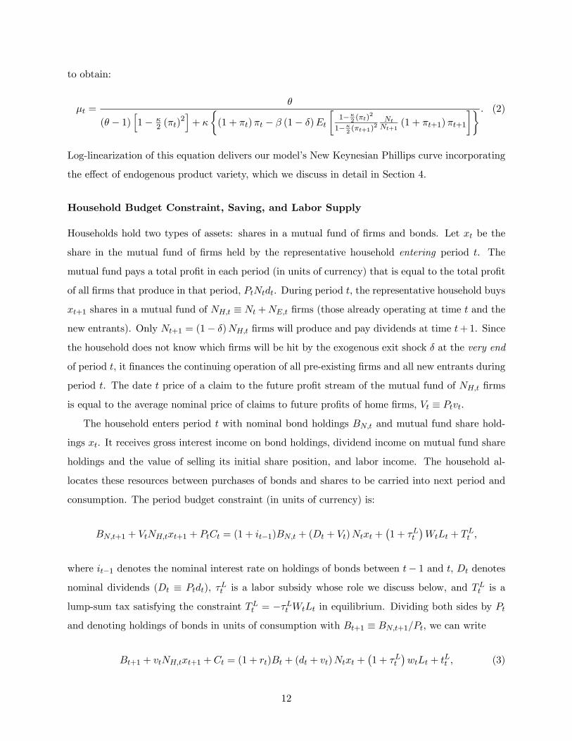
to obtain:

μt =θ

(θ − 1)h1− κ

2 (πt)2i+ κ

½(1 + πt)πt − β (1− δ)Et

∙1−κ

2(πt)

2

1−κ2(πt+1)

2NtNt+1

(1 + πt+1)πt+1

¸¾ . (2)

Log-linearization of this equation delivers our model’s New Keynesian Phillips curve incorporating

the effect of endogenous product variety, which we discuss in detail in Section 4.

Household Budget Constraint, Saving, and Labor Supply

Households hold two types of assets: shares in a mutual fund of firms and bonds. Let xt be the

share in the mutual fund of firms held by the representative household entering period t. The

mutual fund pays a total profit in each period (in units of currency) that is equal to the total profit

of all firms that produce in that period, PtNtdt. During period t, the representative household buys

xt+1 shares in a mutual fund of NH,t ≡ Nt +NE,t firms (those already operating at time t and the

new entrants). Only Nt+1 = (1− δ)NH,t firms will produce and pay dividends at time t+1. Since

the household does not know which firms will be hit by the exogenous exit shock δ at the very end

of period t, it finances the continuing operation of all pre-existing firms and all new entrants during

period t. The date t price of a claim to the future profit stream of the mutual fund of NH,t firms

is equal to the average nominal price of claims to future profits of home firms, Vt ≡ Ptvt.

The household enters period t with nominal bond holdings BN,t and mutual fund share hold-

ings xt. It receives gross interest income on bond holdings, dividend income on mutual fund share

holdings and the value of selling its initial share position, and labor income. The household al-

locates these resources between purchases of bonds and shares to be carried into next period and

consumption. The period budget constraint (in units of currency) is:

BN,t+1 + VtNH,txt+1 + PtCt = (1 + it−1)BN,t + (Dt + Vt)Ntxt +¡1 + τLt

¢WtLt + TL

t ,

where it−1 denotes the nominal interest rate on holdings of bonds between t− 1 and t, Dt denotes

nominal dividends (Dt ≡ Ptdt), τLt is a labor subsidy whose role we discuss below, and TLt is a

lump-sum tax satisfying the constraint TLt = −τLt WtLt in equilibrium. Dividing both sides by Pt

and denoting holdings of bonds in units of consumption with Bt+1 ≡ BN,t+1/Pt, we can write

Bt+1 + vtNH,txt+1 + Ct = (1 + rt)Bt + (dt + vt)Ntxt +¡1 + τLt

¢wtLt + tLt , (3)

12

where 1+ rt is the gross, consumption-based, real interest rate on holdings of bonds between t− 1

and t, defined by 1 + rt ≡ (1 + it−1) /¡1 + πCt

¢, with πCt ≡ Pt/Pt−1 − 1, and tLt ≡ TL

t /Pt. The

home household maximizes its expected intertemporal utility subject to this budget constraint.

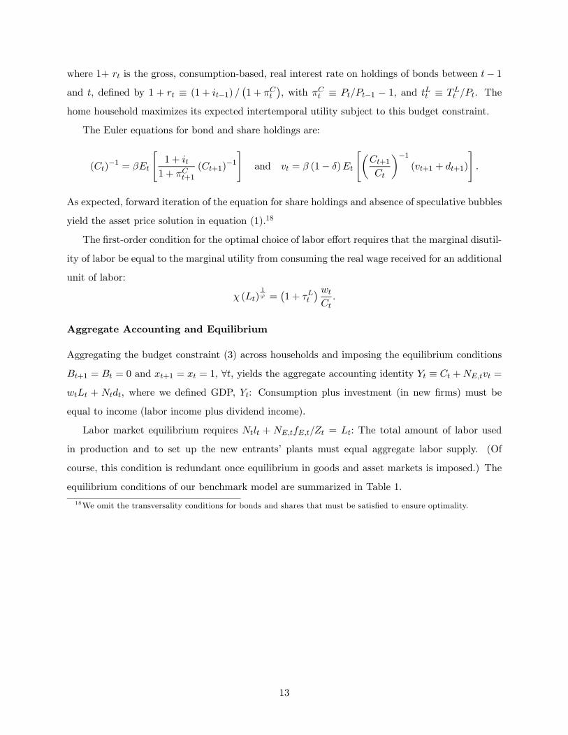
The Euler equations for bond and share holdings are:

(Ct)−1 = βEt

"1 + it

1 + πCt+1(Ct+1)

−1#

and vt = β (1− δ)Et

"µCt+1

Ct

¶−1(vt+1 + dt+1)

#.

As expected, forward iteration of the equation for share holdings and absence of speculative bubbles

yield the asset price solution in equation (1).18

The first-order condition for the optimal choice of labor effort requires that the marginal disutil-

ity of labor be equal to the marginal utility from consuming the real wage received for an additional

unit of labor:

χ (Lt)1ϕ =

¡1 + τLt

¢ wt

Ct.

Aggregate Accounting and Equilibrium

Aggregating the budget constraint (3) across households and imposing the equilibrium conditions

Bt+1 = Bt = 0 and xt+1 = xt = 1, ∀t, yields the aggregate accounting identity Yt ≡ Ct +NE,tvt =

wtLt + Ntdt, where we defined GDP, Yt: Consumption plus investment (in new firms) must be

equal to income (labor income plus dividend income).

Labor market equilibrium requires Ntlt + NE,tfE,t/Zt = Lt: The total amount of labor used

in production and to set up the new entrants’ plants must equal aggregate labor supply. (Of

course, this condition is redundant once equilibrium in goods and asset markets is imposed.) The

equilibrium conditions of our benchmark model are summarized in Table 1.

18We omit the transversality conditions for bonds and shares that must be satisfied to ensure optimality.

13

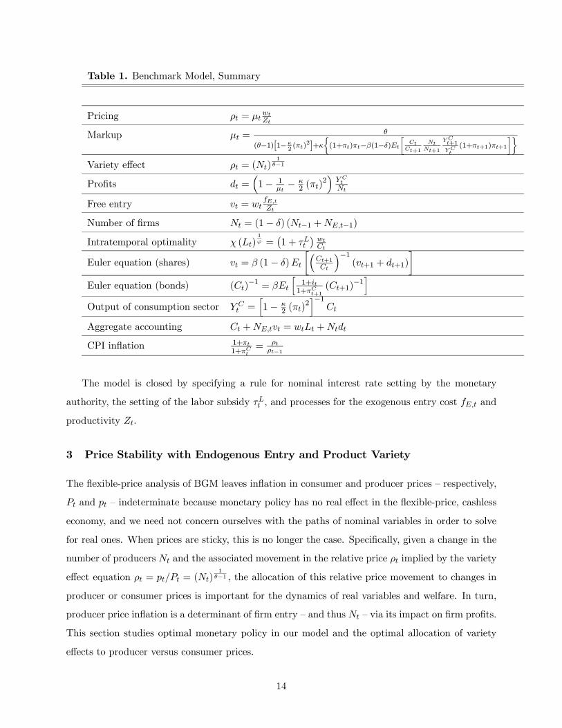
Table 1. Benchmark Model, Summary

Pricing ρt = μtwtZt

Markup μt =θ

(θ−1)[1−κ2(πt)

2]+κ (1+πt)πt−β(1−δ)Et CtCt+1

NtNt+1

Y Ct+1

Y Ct(1+πt+1)πt+1

Variety effect ρt = (Nt)1

θ−1

Profits dt =³1− 1

μt− κ

2 (πt)2´

Y CtNt

Free entry vt = wtfE,tZt

Number of firms Nt = (1− δ) (Nt−1 +NE,t−1)

Intratemporal optimality χ (Lt)1ϕ =

¡1 + τLt

¢wtCt

Euler equation (shares) vt = β (1− δ)Et

∙³Ct+1Ct

´−1(vt+1 + dt+1)

¸Euler equation (bonds) (Ct)

−1 = βEt

h1+it1+πCt+1

(Ct+1)−1i

Output of consumption sector Y Ct =

h1− κ

2 (πt)2i−1

Ct

Aggregate accounting Ct +NE,tvt = wtLt +Ntdt

CPI inflation 1+πt1+πCt

= ρtρt−1

The model is closed by specifying a rule for nominal interest rate setting by the monetary

authority, the setting of the labor subsidy τLt , and processes for the exogenous entry cost fE,t and

productivity Zt.

3 Price Stability with Endogenous Entry and Product Variety

The flexible-price analysis of BGM leaves inflation in consumer and producer prices — respectively,

Pt and pt — indeterminate because monetary policy has no real effect in the flexible-price, cashless

economy, and we need not concern ourselves with the paths of nominal variables in order to solve

for real ones. When prices are sticky, this is no longer the case. Specifically, given a change in the

number of producers Nt and the associated movement in the relative price ρt implied by the variety

effect equation ρt = pt/Pt = (Nt)1

θ−1 , the allocation of this relative price movement to changes in

producer or consumer prices is important for the dynamics of real variables and welfare. In turn,

producer price inflation is a determinant of firm entry — and thus Nt — via its impact on firm profits.

This section studies optimal monetary policy in our model and the optimal allocation of variety

effects to producer versus consumer prices.

14

Our analysis of optimal monetary policy builds on results in Bilbiie, Ghironi, and Melitz (2006).

We show there that the flexible-price version of the economy described above is efficient — the

competitive equilibrium coincides with the social planner’s optimum — if labor supply is inelastic

(ϕ = 0) and Lt = 1 ∀t. The reason is that, with C.E.S. Dixit-Stiglitz preferences, the profit

destruction externality generated by producer entry (which reduces demand for each individual

firm) is exactly matched by the consumer’s love for variety — both determined by the elasticity of

substitution θ. The flexible-price economy is inefficient if ϕ > 0 because there is a misalignment

of markups across the items the consumer cares about (consumption, priced at a markup over

marginal cost, and leisure, priced competitively), but efficiency is restored if the labor subsidy τLt

is equal to the net markup of pricing over marginal cost, 1/ (θ − 1) in all periods. This subsidy

aligns markups across consumption goods and leisure while preserving the expected profitability of

firm entry, thus inducing the efficient equilibrium. We assume that τLt = 1/ (θ − 1) ∀t below.

Sticky prices imply a time-varying markup whenever producer prices are changing over time.

As shown in Bilbiie, Ghironi, and Melitz (2006), markup non-synchronization across periods (as

well as across states and arguments of the utility function) generates inefficiency compared to the

planner’s optimum. Since in this particular model time variation of the markup in the competitive

equilibrium is due to producer price inflation, we expect a zero rate of inflation in producer prices

to be the optimal monetary policy chosen by a planner. The following proposition confirms that

this is indeed the case. To isolate our main result, we prove the proposition for the case of inelastic

labor and then briefly discuss the elastic labor case. As in Bilbiie, Ghironi, and Melitz (2006),

we assume that the planner chooses the amount of labor that is allocated to producing existing

varieties, which, in turn, determines the number of produced varieties. In addition, in this paper,

the planner also chooses the rate of producer price inflation.

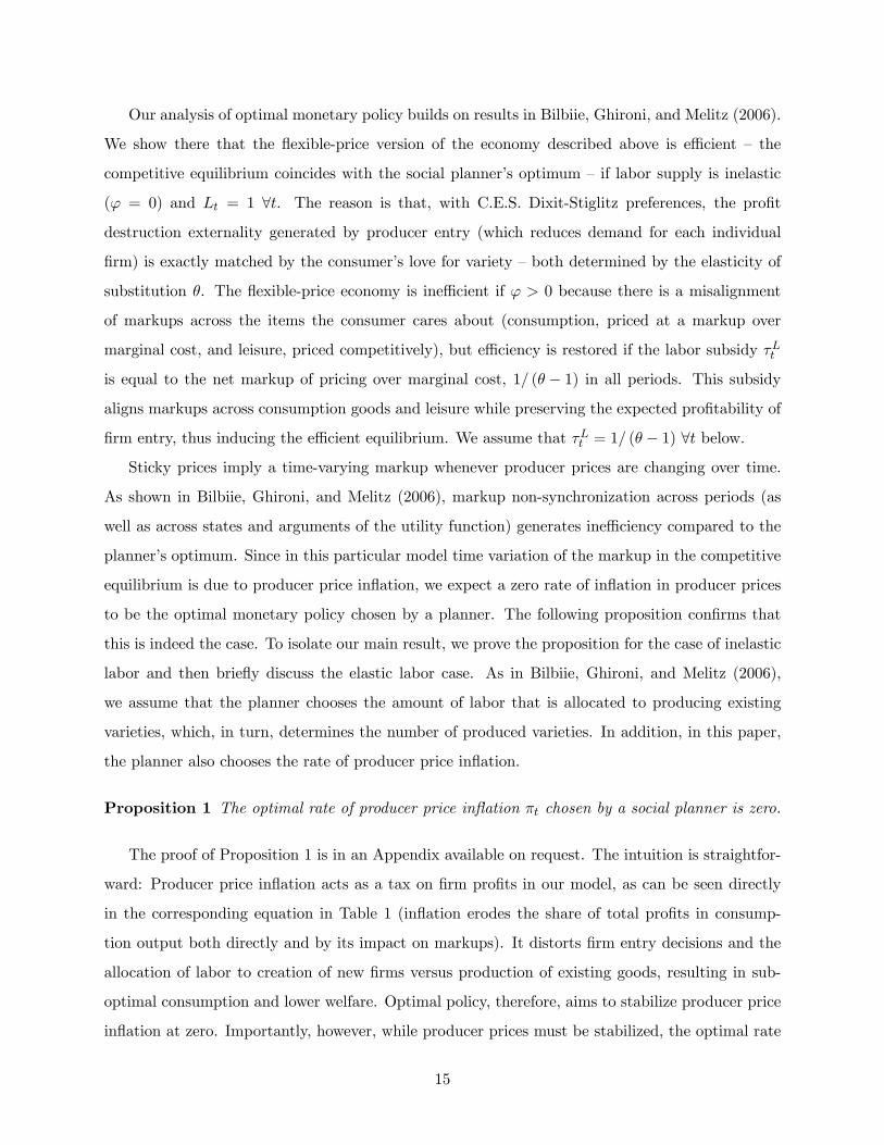
Proposition 1 The optimal rate of producer price inflation πt chosen by a social planner is zero.

The proof of Proposition 1 is in an Appendix available on request. The intuition is straightfor-

ward: Producer price inflation acts as a tax on firm profits in our model, as can be seen directly

in the corresponding equation in Table 1 (inflation erodes the share of total profits in consump-

tion output both directly and by its impact on markups). It distorts firm entry decisions and the

allocation of labor to creation of new firms versus production of existing goods, resulting in sub-

optimal consumption and lower welfare. Optimal policy, therefore, aims to stabilize producer price

inflation at zero. Importantly, however, while producer prices must be stabilized, the optimal rate

15

of consumer price inflation must move freely to accommodate changes in the number of varieties:

1 + πC∗t =

µρ∗tρ∗t−1

¶−1=

µN∗t

N∗t−1

¶− 1θ−1

,

where a star denotes variables in the efficient equilibrium. Given the evidence of bias in the

measurement of CPI inflation (precisely due to poor accounting for new varieties) convincingly

documented by Broda and Weinstein (2006), we view this normative implication of our model as

“good news.” The central bank should target inflation in producer prices rather than (mismeasured)

CPI inflation.

When labor supply is elastic, the subsidy τLt = 1/ (θ − 1) ensures that the flexible-price equilib-

rium is efficient, removing the wedge otherwise present between the marginal rates of substitution

and transformation between consumption and leisure. In this case, price stickiness distorts both

the total amount of labor supplied and its allocation to creation of new firms and production of

existing goods. It is easy to verify that a zero rate of inflation in producer prices is still the optimal

monetary policy.

The optimality of producer price stability with inelastic labor supply highlights a new argument

for price stability (at the producer level) implied by endogenous entry and product variety. In a

model with exogenously fixed number of firms and inelastic labor supply, time variation in the

markup would have no impact on the equilibrium path of consumption and welfare: Consumption

would be simply determined by the exogenous productivity and labor supply regardless of markup

dynamics. Endogenous entry and product variety imply that markup variation reduces welfare by

distorting entry decisions and the allocation of the fixed amount of labor to firm creation versus

production of existing goods. This introduces a role for monetary policy in welfare maximization by

stabilizing producer price inflation at zero — and the markup at its flexible-price level. We discuss

implementation of the optimal monetary policy by setting the nominal interest rate below.

4 The New Keynesian Phillips Curve and the Log-Linear Model

This section describes the implications of endogenous entry and product variety for the New Key-

nesian Phillips curve and presents the key log-linear equations of the model.

16

The New Keynesian Phillips Curve

To study the propagation of shocks and compute second moments of the endogenous variables

implied by assumptions on the processes for exogenous shocks, we log-linearize the model around the

efficient steady state with zero inflation under assumptions of log-normality and homoskedasticity.

We denote percent deviations from steady state with sans serif fonts. Our model’s version of the

New Keynesian Phillips curve follows from log-linearizing equation (2):

πt = β (1− δ)Etπt+1 −θ − 1κ

μt, (4)

where πt and μt now denote percent deviations from steady state (of gross inflation in the case of

πt).

Since ρt = pt/Pt = (Nt)1

θ−1 and optimal firm pricing implies μt = ρt/λt = ρtZt/wt, it follows

that μt = (Nt)1

θ−1 Zt/wt, or, in log-linear terms:

μt =1

θ − 1Nt − (wt − Zt) . (5)

(With a constant number of firms, this relation reduces to the familiar negative relation between

markup and marginal cost of the benchmark New Keynesian model.) Substituting (5) into (4)

yields:

πt = β (1− δ)Etπt+1 +θ − 1κ

(wt − Zt)−1

κNt. (6)

Equation (6) is a New Keynesian Phillips curve relation that ties firm-level inflation dynamics to

marginal cost in a standard fashion. Importantly, the effect of marginal cost is adjusted to reflect

the number of producers that operate in the economy. This is a predetermined, state variable, which

introduces directly a degree of endogenous persistence in the dynamics of product price inflation

in the Phillips curve.

Furthermore, our model links the dynamics of inflation to asset prices in an endogenous way,

as can be seen by combining (6) with the log-linear free entry condition to obtain:

πt = β (1− δ)Etπt+1 +θ − 1κ

(vt − fE,t)−1

κNt. (7)

This equation ties inflation dynamics to the relative price of investment in new firms. It stipulates

that, for given expected inflation and number of firms, inflation is positively related to equity prices.

17

Together with the no-arbitrage condition between bonds and equity implied by optimal household

behavior, this connection between inflation and equity prices (and thus capital accumulation in our

model) plays a crucial role for the determinacy and stability properties of interest rate setting that

we discuss below.

Finally, using the definition of CPI inflation, we can write the New Keynesian Phillips curve

for consumption-based inflation:

πCt = β (1− δ)EtπCt+1 +

θ − 1κ

(wt − Zt)−1

κNt −

1

θ − 1 [Nt − Nt−1 − β (1− δ) (Nt+1 −Nt)] , (8)

where πCt now denotes the percent deviation of the gross CPI inflation rate from the steady state.

Consumption-based inflation displays an additional degree of endogenous persistence relative to

firm-level inflation in that it depends directly on the number of firms that produced at time t− 1,

which was determined in period t− 2.

Implications for Empirical Exercises

Existing empirical studies estimating the New Keynesian Phillips curve (4), such as Sbordone (2002)

and Galí and Gertler (1999), proxy the (unobservable) markup variable with the inverse of the labor

share. This is an approximation that holds exactly in a model without endogenous variety. In our

model with endogenous variety, however, this relationship no longer holds. Indeed, if one believes

product variety to be important for business cycles, the proxy for the markup that one should

use is the inverse of the share of labor (in consumption output) beyond the ‘overhead’ quantity

(from an aggregate perspective) used to set up new product lines, μt = Y Ct / [wt (Lt − LE,t)] . This

markup measure corresponds closely to the labor share measure used by Rotemberg and Woodford

(1999) that takes into account overhead labor. Log-linearization of this equation, when replaced

into (4), delivers a relation that is testable empirically.19 Alternatively, exploiting the equation

for profits, one could use the inverse of (one minus) the profit share, μt =¡1−DG

t /YCt

¢−1, as aproxy for markups, where DG

t ≡ dtNt+κ2 (πt)

2 Y Ct are profits gross of the costs of price adjustment.

Note that since these costs are zero when log-linearizing around a zero-inflation steady-state (and

hence consumption is equal to consumption output and gross profits are equal to net profits), the

19Sbordone (2002) indeed showed that using this corrected measure does not affect the estimates obtained whenusing the baseline markup proxy. Our framework suggests a specific calibration scheme for the share of overheadlabor used in this correction, namely: LE/L = δ (μ− 1) / (r + δμ), where we denote steady-state levels of variablesby dropping the subscript t. Under our baseline parametrization below, this is approximately 0.20; the upper boundsuggested by the empirical results of Basu and Kimball (1997) is 0.25.

18

empirically usable equation will feature only observable variables, i.e., consumption and total profit

receipts (or dividends).20

A further implication of our framework for empirical exercises comes from the natural distinc-

tion between consumer and producer price inflation in our model: Our framework implies that,

in order to overcome measurement issues inherent in using CPI inflation, empirical studies of the

Phillips curve should concentrate on producer price inflation (which is also the relevant objective

for monetary policy). Construction of CPI data by statistical agencies does not adjust for availabil-

ity of new varieties in the specific functional form dictated by the welfare-consistent price index.

Furthermore, adjustment for variety, when it happens, certainly does not happen at the frequency

represented by periods in our model. Actual CPI data are closer to pt (the average price level in our

economy) than Pt. For this reason, when investigating the properties of the model in relation to the

data (for instance, when computing second moments below or in the specification of policy rules

that allow for reaction to measured real quantities), one should focus on real variables deflated

by a data-consistent price index. For any variable Xt in units of the consumption basket, such

data-consistent counterpart is obtained as XR,t ≡ PtXt/pt = Xt/ρt.21

Related to this measurement issue, our framework implies an ‘endogeneity bias’ in cost-push

shocks in much empirical literature on the New Keynesian Phillips curve. An endogenous term

that depends on Nt (due the measurement bias from not accounting for variety) is attributed to

exogenous cost-push shocks when estimating the Phillips curve equation (6) using a proxy for

marginal cost without variety.

When the variety effect is removed from the welfare-consistent equity price, the Phillips curve

(7) becomes:

πt = β (1− δ)Etπt+1 +θ − 1κ

(vR,t − fE,t) , (9)

where vR,t is the value of the firm/price of shares net of the variety effect. For given expectations

of future inflation, actual inflation is increasing in the data-consistent price of equity.

20We leave estimation of Phillips curves using these alternative profit-based proxies for the markup for futureresearch.21Returning to the normative prescription that the central bank should stabilize producer prices, our model implies

that if the central bank targeted CPI inflation, the bias in its measurement would indeed be beneficial to the extentthat biased CPI inflation is closer to producer price inflation than welfare-consistent consumer price inflation.

19

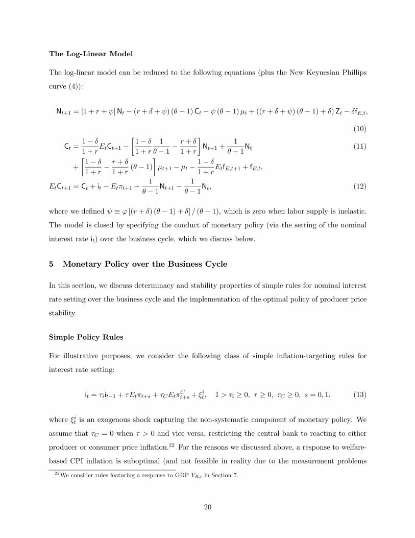
The Log-Linear Model

The log-linear model can be reduced to the following equations (plus the New Keynesian Phillips

curve (4)):

Nt+1 = [1 + r + ψ]Nt − (r + δ + ψ) (θ − 1)Ct − ψ (θ − 1)μt + ((r + δ + ψ) (θ − 1) + δ)Zt − δfE,t,

(10)

Ct =1− δ

1 + rEtCt+1 −

∙1− δ

1 + r

1

θ − 1 −r + δ

1 + r

¸Nt+1 +

1

θ − 1Nt (11)

+

∙1− δ

1 + r− r + δ

1 + r(θ − 1)

¸μt+1 − μt −

1− δ

1 + rEtfE,t+1 + fE,t,

EtCt+1 = Ct + it −Etπt+1 +1

θ − 1Nt+1 −1

θ − 1Nt, (12)

where we defined ψ ≡ ϕ [(r + δ) (θ − 1) + δ] / (θ − 1), which is zero when labor supply is inelastic.

The model is closed by specifying the conduct of monetary policy (via the setting of the nominal

interest rate it) over the business cycle, which we discuss below.

5 Monetary Policy over the Business Cycle

In this section, we discuss determinacy and stability properties of simple rules for nominal interest

rate setting over the business cycle and the implementation of the optimal policy of producer price

stability.

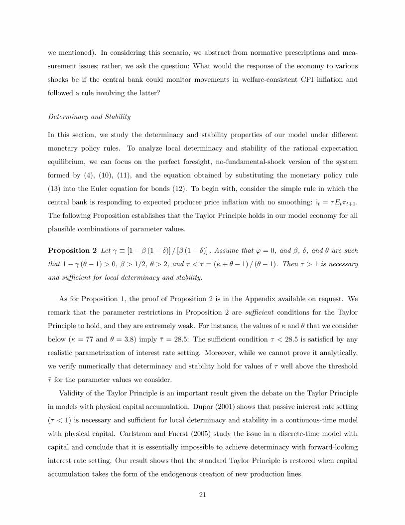
Simple Policy Rules

For illustrative purposes, we consider the following class of simple inflation-targeting rules for

interest rate setting:

it = τiit−1 + τEtπt+s + τCEtπCt+s + ξit, 1 > τi ≥ 0, τ ≥ 0, τC ≥ 0, s = 0, 1. (13)

where ξit is an exogenous shock capturing the non-systematic component of monetary policy. We

assume that τC = 0 when τ > 0 and vice versa, restricting the central bank to reacting to either

producer or consumer price inflation.22 For the reasons we discussed above, a response to welfare-

based CPI inflation is suboptimal (and not feasible in reality due to the measurement problems

22We consider rules featuring a response to GDP YR,t in Section 7.

20

we mentioned). In considering this scenario, we abstract from normative prescriptions and mea-

surement issues; rather, we ask the question: What would the response of the economy to various

shocks be if the central bank could monitor movements in welfare-consistent CPI inflation and

followed a rule involving the latter?

Determinacy and Stability

In this section, we study the determinacy and stability properties of our model under different

monetary policy rules. To analyze local determinacy and stability of the rational expectation

equilibrium, we can focus on the perfect foresight, no-fundamental-shock version of the system

formed by (4), (10), (11), and the equation obtained by substituting the monetary policy rule

(13) into the Euler equation for bonds (12). To begin with, consider the simple rule in which the

central bank is responding to expected producer price inflation with no smoothing: it = τEtπt+1.

The following Proposition establishes that the Taylor Principle holds in our model economy for all

plausible combinations of parameter values.

Proposition 2 Let γ ≡ [1− β (1− δ)] / [β (1− δ)] . Assume that ϕ = 0, and β, δ, and θ are such

that 1− γ (θ − 1) > 0, β > 1/2, θ > 2, and τ < τ = (κ+ θ − 1) / (θ − 1). Then τ > 1 is necessary

and sufficient for local determinacy and stability.

As for Proposition 1, the proof of Proposition 2 is in the Appendix available on request. We

remark that the parameter restrictions in Proposition 2 are sufficient conditions for the Taylor

Principle to hold, and they are extremely weak. For instance, the values of κ and θ that we consider

below (κ = 77 and θ = 3.8) imply τ = 28.5: The sufficient condition τ < 28.5 is satisfied by any

realistic parametrization of interest rate setting. Moreover, while we cannot prove it analytically,

we verify numerically that determinacy and stability hold for values of τ well above the threshold

τ for the parameter values we consider.

Validity of the Taylor Principle is an important result given the debate on the Taylor Principle

in models with physical capital accumulation. Dupor (2001) shows that passive interest rate setting

(τ < 1) is necessary and sufficient for local determinacy and stability in a continuous-time model

with physical capital. Carlstrom and Fuerst (2005) study the issue in a discrete-time model with

capital and conclude that it is essentially impossible to achieve determinacy with forward-looking

interest rate setting. Our result shows that the standard Taylor Principle is restored when capital

accumulation takes the form of the endogenous creation of new production lines.

21

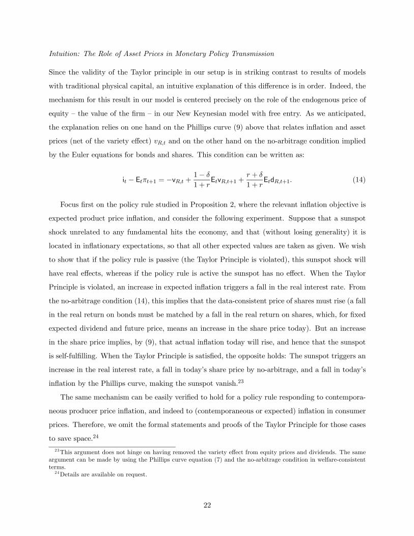
Intuition: The Role of Asset Prices in Monetary Policy Transmission

Since the validity of the Taylor principle in our setup is in striking contrast to results of models

with traditional physical capital, an intuitive explanation of this difference is in order. Indeed, the

mechanism for this result in our model is centered precisely on the role of the endogenous price of

equity — the value of the firm — in our New Keynesian model with free entry. As we anticipated,

the explanation relies on one hand on the Phillips curve (9) above that relates inflation and asset

prices (net of the variety effect) vR,t and on the other hand on the no-arbitrage condition implied

by the Euler equations for bonds and shares. This condition can be written as:

it − Etπt+1 = −vR,t +1− δ

1 + rEtvR,t+1 +

r + δ

1 + rEtdR,t+1. (14)

Focus first on the policy rule studied in Proposition 2, where the relevant inflation objective is

expected product price inflation, and consider the following experiment. Suppose that a sunspot

shock unrelated to any fundamental hits the economy, and that (without losing generality) it is

located in inflationary expectations, so that all other expected values are taken as given. We wish

to show that if the policy rule is passive (the Taylor Principle is violated), this sunspot shock will

have real effects, whereas if the policy rule is active the sunspot has no effect. When the Taylor

Principle is violated, an increase in expected inflation triggers a fall in the real interest rate. From

the no-arbitrage condition (14), this implies that the data-consistent price of shares must rise (a fall

in the real return on bonds must be matched by a fall in the real return on shares, which, for fixed

expected dividend and future price, means an increase in the share price today). But an increase

in the share price implies, by (9), that actual inflation today will rise, and hence that the sunspot

is self-fulfilling. When the Taylor Principle is satisfied, the opposite holds: The sunspot triggers an

increase in the real interest rate, a fall in today’s share price by no-arbitrage, and a fall in today’s

inflation by the Phillips curve, making the sunspot vanish.23

The same mechanism can be easily verified to hold for a policy rule responding to contempora-

neous producer price inflation, and indeed to (contemporaneous or expected) inflation in consumer

prices. Therefore, we omit the formal statements and proofs of the Taylor Principle for those cases

to save space.24

23This argument does not hinge on having removed the variety effect from equity prices and dividends. The sameargument can be made by using the Phillips curve equation (7) and the no-arbitrage condition in welfare-consistentterms.24Details are available on request.

22

A comparison of our results and intuition with those of Carlstrom and Fuerst (2005) allows us to

further emphasize the crucial role of the different type of capital at the core of our model. Carlstrom

and Fuerst show that indeterminacy occurs in a discrete-time model with physical capital when

the central bank responds to expected future inflation because the no-arbitrage condition between

bonds and capital contains no variable dated at time t. This happens because the expected return

to capital depends only on future variables determining the marginal product of capital at time

t + 1. In turn, this implies that there is a zero root in the system, and indeterminacy.25 Instead,

in our model, the expected return on shares depends on the price of shares today (an endogenous

variable), hence removing this ‘zero-root’ problem. Indeed, through today’s price of equity, our

model provides a novel link between the no-arbitrage condition and the Phillips curve that is

absent in models that do not feature endogenous variety and free entry.

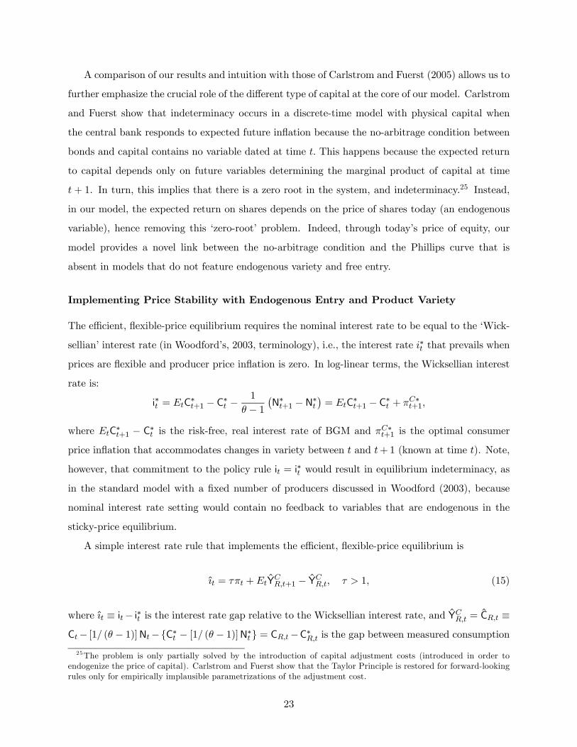
Implementing Price Stability with Endogenous Entry and Product Variety

The efficient, flexible-price equilibrium requires the nominal interest rate to be equal to the ‘Wick-

sellian’ interest rate (in Woodford’s, 2003, terminology), i.e., the interest rate i∗t that prevails when

prices are flexible and producer price inflation is zero. In log-linear terms, the Wicksellian interest

rate is:

i∗t = EtC∗t+1 − C∗t −

1

θ − 1¡N∗t+1 − N∗t

¢= EtC

∗t+1 − C∗t + πC∗t+1,

where EtC∗t+1 − C∗t is the risk-free, real interest rate of BGM and πC∗t+1 is the optimal consumer

price inflation that accommodates changes in variety between t and t+1 (known at time t). Note,

however, that commitment to the policy rule it = i∗t would result in equilibrium indeterminacy, as

in the standard model with a fixed number of producers discussed in Woodford (2003), because

nominal interest rate setting would contain no feedback to variables that are endogenous in the

sticky-price equilibrium.

A simple interest rate rule that implements the efficient, flexible-price equilibrium is

ıt = τπt +EtYCR,t+1 − YCR,t, τ > 1, (15)

where ıt ≡ it− i∗t is the interest rate gap relative to the Wicksellian interest rate, and YCR,t = CR,t ≡

Ct− [1/ (θ − 1)]Nt−C∗t − [1/ (θ − 1)]N∗t = CR,t−C∗R,t is the gap between measured consumption25The problem is only partially solved by the introduction of capital adjustment costs (introduced in order to

endogenize the price of capital). Carlstrom and Fuerst show that the Taylor Principle is restored for forward-lookingrules only for empirically implausible parametrizations of the adjustment cost.

23

output and its flexible-price level. The interest rate rule (15) requires the monetary authority to

track changes in the Wicksellian interest rate and in expected growth of the consumption output

gap, and to respond more than proportionally to inflation. It is possible to verify that the following

equation holds for the dynamics of the consumption output gap:

EtYCR,t+1 − YCR,t = ıt −Etπt+1.

Substituting the interest rate rule (15) into this equation yields τπt = Etπt+1, which has unique

solution πt = 0 ∀t since the Taylor Principle is satisfied. In turn, zero producer price inflation in

all periods implies YCR,t = 0, and, therefore, it = i∗t ∀t.26

6 Business Cycles: Propagation and Second Moments

In this section, we explore the properties of our benchmark model by means of numerical examples.

We compute impulse responses to productivity, deregulation, and monetary policy shocks. Next,

we compute second moments of our artificial economy and compare them to second moments in the

data and those produced by the baseline BGM model with flexible prices and C.E.S. preferences.

As shown in BGM, these moments (which also correspond to those under the optimal monetary

policy in the sticky-price economy) are very close to those generated by the standard RBC model.

Calibration

In our baseline calibration, we interpret periods as quarters and set β = 0.99 — a standard choice

for quarterly business cycle models. We set the size of the exogenous firm exit shock δ = 0.025 to

match the U.S. empirical level of 10 percent job destruction per year.27 We use the value of θ from

Bernard, Eaton, Jensen, and Kortum (2003) and set θ = 3.8, which was calibrated to fit U.S. plant

and macro trade data.28 We set initial productivity to Z = 1. The initial steady-state entry cost

26Rule (15) is by no means the only interest rate rule that implements the optimal monetary policy. It is of coursepossible to design alternative rules that achieve this goal.27Empirically, job destruction is induced by both firm exit and contraction. In our model, the “death” shock δ

takes place at the product level. In a multi-product firm, the disappearance of a product generates job destructionwithout firm exit. Since we abstract from the explicit modeling of multi-product firms, we include this portion of jobdestruction in δ. As a higher δ implies less persistent dynamics, our choice of δ is also consistent with not overstatingthe ability of the model to generate persistence.28 It may be argued that the value of θ results in a steady-state markup that is too high relative to the evidence.

However, it is important to observe that, in models without any fixed cost, θ/ (θ − 1) is a measure of both markupover marginal cost and average cost. In our model with entry costs, free entry ensures that firms earn zero profitsnet of the entry cost. This means that firms price at average cost (inclusive of the entry cost). Thus, althoughθ = 3.8 implies a fairly high markup over marginal cost, our parametrization delivers reasonable results with respect

24

fE does not affect any impulse response; we therefore set fE = 1 without loss of generality. We

consider different values for the elasticity of labor supply, ϕ, and we set the weight of the disutility

of labor in the period utility function, χ, so that the steady-state level of labor effort is 1 — and

steady-state levels of all variables are the same — regardless of ϕ.29 We set the price stickiness

parameter κ = 77, the value estimated by Ireland (2001). Although Ireland obtained this estimate

using a different model, without entry and endogenous variety, our results are not sensitive to

changes in the value of this parameter within a plausible range.

Impulse Responses

Productivity

Figure 1 shows the responses (percent deviations from steady state) to a 1 percent increase in

productivity for the inelastic labor case. For consistence with the second moment results below,

we assume productivity persistence 0.979 as in King and Rebelo (1999). The figure compares the

efficient flexible-price equilibrium obtained under optimal monetary policy (blue, round markers)

with three alternative parametrizations of the monetary policy rule (13). The first is a simple rule

responding to expected producer price inflation, it = 1.5Etπt+1 (red, cross markers); the second is

a rule involving interest rate smoothing, it = 0.8it−1 + 0.3Etπt+1 (green, square markers), which

features the same long-run response to expected inflation (1.5) as the previous rule; and the third is

a rule responding to expected welfare-consistent CPI inflation, it = 1.5EtπCt+1 (pink, star markers).

Note that the difference between the responses under each of the simple rules and the optimal

policy measures the gap relative to the flexible-price equilibrium under the alternative rules. The

number of years after the shock is on the horizontal axis, and responses are normalized so that 0.3

(for instance) denotes 0.3 percent.

Focus on the responses under the optimal policy. The increase in productivity makes the

business environment temporarily more attractive, drawing a higher number of entrants (NE,t),

which translates into a gradual increase in the number of producers (Nt) before entry and the stock

of production lines return to the steady state. The larger number of producers induces marginal

cost (wt/Zt — not shown) and the relative price of each product ρt to increase gradually with

unchanged markup. GDP (Yt) and consumption (Ct) increase, and so does investment in new firms

to pricing and average costs. The main qualitative features of the impulse responses below are not affected if we setθ = 6, resulting in a 20 percent markup of price over marginal cost as in Rotemberg and Woodford (1992) and severalother studies.29This requires χ = 0.924271.

25

(vEt ≡ vtNE,t) as the fixed labor supply is reallocated toward creation of new products. Interestingly,

firm-level output (yt) is below the steady state during most of the transition, except for an initial

expansion. The effect of a higher relative price prevails on the expansion in consumption demand

to push individual firm output below the steady state for much of the transition, with expansion

in the number of producers and investment in new firms responsible for GDP remaining above the

steady state throughout the transition. Notably, the dynamics of firm entry result in responses

that persist beyond the duration of the exogenous shock, and, for some key variables, display a

hump-shaped pattern.30

When comparing responses across policy rules, a remarkable feature of the results is that the

dynamics of macroeconomic aggregates under the first two simple policy rules are strikingly similar

to those in the flexible-price equilibrium. Indeed, the responses of GDP are virtually indistinguish-

able, and those of consumption and the number of producers are also very close. Equivalently, the

changes in producer price inflation and the markup induced by technology shocks under these pol-

icy rules are small. It is worth stressing that this is in contrast with responses in the fixed-variety,

benchmark New Keynesian model, where there are quantitatively significant deviations from the

flexible-price equilibrium under such simple policy rules. In our model, instead, a simple rule such

as it = 1.5Etπt+1, despite not featuring an overly aggressive response to inflation, manages to bring

the economy quite close to its first-best optimum. This is no longer true when monetary policy

responds to welfare-consistent CPI inflation: There are more evident differences in the responses

of consumption and the number of producers, stemming from the suboptimal response of the cen-

tral bank to movements in welfare-based CPI inflation that reflect fluctuations in the number of

products.31

Importantly, our model with entry can induce inflation and countercyclical markups, and po-

tentially procyclical labor, in response to technology shocks. To understand this result, recall the

intuition in the standard New Keynesian model, which implies deflation and procyclical markups in

response to productivity increases: Marginal cost falls, prices decrease (there is deflation), but not

by as much because of stickiness, so output increases and markups increase too — i.e., the markup is

procyclical. In our model with entry, there is an additional channel of shock transmission working

in the opposite direction: Positive productivity shocks increase future profits and the value of the

30The responses of several macroeconomic variables deflated by average prices (the producer price level pt) ratherthan with the consumption-based price index are qualitatively similar. For instance, CR,t increases, with a hump-shaped response except when policy responds to welfare-based CPI inflation. YR,t also rises, although without ahump.31Results from policy rules featuring a response to GDP are available on request.

26

firm (it is more productive to create new goods). Entry puts pressure on labor demand, inducing

marginal cost to increase in order to satisfy free entry. By this channel, prices increase, but not by

as much, and output increases (both consumption and investment increase). There is inflation and

the markup is countercyclical. Otherwise put, through the usual channel, labor demand by existing

firms falls, the real wage falls, and the markup increases. Through the new channel, labor demand

by entrants increases and, if it increases enough, it can overturn the usual effect and generate an

increase in total labor demand, a higher real wage, and a countercyclical markup. Which channel

dominates depends on parameter values (for instance, shock persistence). As shown in Figure 1,

the new channel dominates on impact with the persistence that we use to compute second moments

below.

Deregulation

Figure 2 shows the responses to a 1 percent, permanent deregulation shock (a lowering of the entry

cost fE,t) with inelastic labor supply under the same policy scenarios as above.

Focus again on responses under the optimal policy. Deregulation attracts new entrants and

firm value decreases (the relative price of the investment good falls). Since investment is relatively

more attractive than consumption, there is intersectoral labor reallocation from the latter to the

former. Consumption falls initially as households now postpone consumption to invest more in firms

whose productivity has not increased. The number of firms starts increasing, but GDP initially

falls as the decline in consumption dominates the increase in investment. All variables then move

monotonically toward their new steady-state levels. A consequence of C.E.S. preferences is that

the long run expansion of consumption is entirely driven by the extensive margin (the long-run

increase in the number of producers), with output per firm back at the initial steady-state level.

As in the case of a productivity shock, the responses for the first two alternative policy rules,

where the targeted measure of inflation is producer price inflation, are again very similar to the

flexible-price responses. As for productivity, the difference is larger when the monetary authority

responds to welfare-based CPI inflation, for the same reasons discussed above. The most notable

difference with respect to the flexible-price case in all responses (but more so when the rule responds

to welfare-based CPI inflation) concerns the dynamics of the consumer price index. Under the

optimal policy, deregulation induces deflation in the welfare-based CPI (at a decreasing rate in

absolute terms) precisely because there is an increase in the number of products (at a decreasing

rate). Under the alternative rules, this response changes sign, positive inflation in the welfare-based

27

CPI occurs, because the increase in producer price inflation is high enough to compensate the effect

of the increase in the number of available varieties. This effect is strongest when the central bank

responds to welfare-based CPI inflation.

Monetary Policy

The next set of responses, plotted in Figure 3, shows the effects of a purely transitory shock to

the nominal interest rate — a 1 percent decrease with zero exogenous persistence. Because of

the assumption of zero exogenous persistence, all responses are plotted for the policy rule involving

interest rate smoothing (otherwise, the effect of the shock is very short-lived), but for different values

of the labor supply elasticity, ϕ = 0, 2, and 4, respectively.32 An interest rate cut generates inflation

and a positive response of GDP (as measured both by Yt and the data-consistent counterpart, YR,t).

Wages rise, consistent with conventional wisdom and the bulk of empirical evidence for the post-

1980 U.S. (for instance, Christiano, Eichenbaum, and Evans, 1999). However, the expansionary

effect on GDP is combined with a contractionary impact effect on entry (and a gradual decrease in

the number of producers) that conflicts with the evidence in Bergin and Corsetti (2005) and Lewis

(2006).33 The fall in the number of entrants occurs because no-arbitrage requires the expected

return on equity to fall along with the ex ante real return on bonds. The decrease in the expected

return on equity is brought about by an increase in the price of shares today relative to the future:

The procyclical impact response of the real wage translates into an increase in today’s equity price

via the free entry condition. The cost of firm creation — which requires labor — increases, and its

expected return falls, inducing investment in new products to fall (the combination of prices that

the household faces makes it relatively more attractive to consume rather than invest). This effect

changes sign after a few years, when the real wage falls and share prices are below the steady state,

making it attractive to invest in product creation. The contractionary effect of monetary expansions

on entry relies crucially on the link between firm value and marginal cost implied by free entry. In

Section 7, we study a version of the model that breaks this link and implies an expansionary effect

of monetary policy expansions on firm entry.34

32The inelastic labor case is in blue (round markers); ϕ = 2 is in red (cross markers); and ϕ = 4 is in green (squaremarkers).33Note, however, that Bergin and Corsetti find that unconditional correlations between a measure of expansionary

monetary policy and measures of entry (gross or net) are negative.34We should note, however, that if the economy started from a situation of zero entry (in which the free entry

condition holds with inequality, v < wfE/Z, and NE = 0), a strong enough monetary expansion could induce anincrease in share prices that brings the economy to the ‘entry’ region studied in this paper (in which the entrycondition holds with equality and there is a positive mass of entrants at all times). In that case, expansionary

28

Second Moments

To further evaluate the properties of the sticky-price model, we compute the implied unconditional

second moments of our artificial economy for some key macroeconomic variables and compare them

to those of the data and those produced by the BGM flexible-price model with C.E.S. preferences.

In this exercise, we focus on random shocks to Zt as the source of business cycle fluctuations,

assuming that sunk entry costs are constant at fE,t = 1 and abstracting from exogenous monetary

policy shocks.35 To start with, we compute moments of GDP, consumption, investment, and hours

worked. We use the same productivity process as King and Rebelo (1999), with persistence 0.979

and a standard deviation of innovations equal to 0.0072, to facilitate comparison of results with the

baseline RBC setup and BGM. As in King and Rebelo’s benchmark calibration, we set ϕ = 2.36

Under sticky prices, we assume that monetary policy follows the rule it = 0.8it−1+0.3Etπt+1. This

rule is empirically plausible based on the findings of a large empirical literature, which documents

the importance of interest rate smoothing in Federal Reserve policy, its focus on inflation targeting

since the 1980s, and the marginal significance of GDP responses. Table 2 presents the results.

For each moment, the first number (bold fonts) is the empirical moment implied by the U.S. data

reported in King and Rebelo (1999), the second number (normal fonts) is the moment generated

by the flexible-price model (or optimal monetary policy under sticky prices), and the third number

(italics) is the moment generated by the sticky-price model under the rule above. We compute

model-implied second moments for HP-filtered variables for consistency with data and standard

RBC practice, and we measure investment in our model with the real value of household investment

in new firms (vR,tNE,t).

monetary policy would have an expansionary effect on entry also in this version of the model.35The empirical literature has downplayed the role of exogenous monetary policy as a source of fluctuations, focusing

instead on the role of systematic policy in response to economic conditions as a mechanism for propagation of thecycle. See, for instance, Leeper, Sims, and Zha (1996).36The period utility function is defined over leisure (1− Lt) in King and Rebelo (1999), where the endowment of

time in each period is normalized to 1. The elasticity of labor supply is then the risk aversion to variations in leisure(set to 1 in their benchmark calibration) multiplied by (1 − L)/L, where L is steady-state effort, calibrated to 1/3.This yields ϕ = 2 in our specification.

29

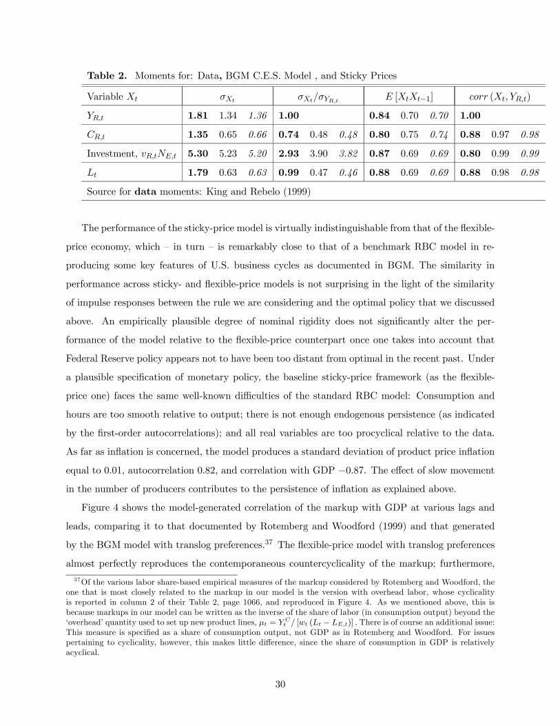
Table 2. Moments for: Data, BGM C.E.S. Model , and Sticky Prices

Variable Xt σXt σXt/σYR,t E [XtXt−1] corr (Xt, YR,t)

YR,t 1.81 1.34 1.36 1.00 0.84 0.70 0.70 1.00

CR,t 1.35 0.65 0.66 0.74 0.48 0.48 0.80 0.75 0.74 0.88 0.97 0.98

Investment, vR,tNE,t 5.30 5.23 5.20 2.93 3.90 3.82 0.87 0.69 0.69 0.80 0.99 0.99

Lt 1.79 0.63 0.63 0.99 0.47 0.46 0.88 0.69 0.69 0.88 0.98 0.98

Source for data moments: King and Rebelo (1999)

The performance of the sticky-price model is virtually indistinguishable from that of the flexible-

price economy, which — in turn — is remarkably close to that of a benchmark RBC model in re-

producing some key features of U.S. business cycles as documented in BGM. The similarity in

performance across sticky- and flexible-price models is not surprising in the light of the similarity

of impulse responses between the rule we are considering and the optimal policy that we discussed

above. An empirically plausible degree of nominal rigidity does not significantly alter the per-

formance of the model relative to the flexible-price counterpart once one takes into account that

Federal Reserve policy appears not to have been too distant from optimal in the recent past. Under

a plausible specification of monetary policy, the baseline sticky-price framework (as the flexible-

price one) faces the same well-known difficulties of the standard RBC model: Consumption and

hours are too smooth relative to output; there is not enough endogenous persistence (as indicated

by the first-order autocorrelations); and all real variables are too procyclical relative to the data.

As far as inflation is concerned, the model produces a standard deviation of product price inflation

equal to 0.01, autocorrelation 0.82, and correlation with GDP −0.87. The effect of slow movement

in the number of producers contributes to the persistence of inflation as explained above.

Figure 4 shows the model-generated correlation of the markup with GDP at various lags and

leads, comparing it to that documented by Rotemberg and Woodford (1999) and that generated

by the BGM model with translog preferences.37 The flexible-price model with translog preferences

almost perfectly reproduces the contemporaneous countercyclicality of the markup; furthermore,

37Of the various labor share-based empirical measures of the markup considered by Rotemberg and Woodford, theone that is most closely related to the markup in our model is the version with overhead labor, whose cyclicalityis reported in column 2 of their Table 2, page 1066, and reproduced in Figure 4. As we mentioned above, this isbecause markups in our model can be written as the inverse of the share of labor (in consumption output) beyond the‘overhead’ quantity used to set up new product lines, μt = Y C

t / [wt (Lt − LE,t)] . There is of course an additional issue:This measure is specified as a share of consumption output, not GDP as in Rotemberg and Woodford. For issuespertaining to cyclicality, however, this makes little difference, since the share of consumption in GDP is relativelyacyclical.

30

the time profile of its correlation with the business cycle is very similar to that documented by

Rotemberg and Woodford. The markup is countercyclical with translog preferences because the

elasticity of substitution across goods is tied to the number of producers, which increases during

expansions. The time profile of the correlation is due to the slow response of the stock of producers

to shocks, with GDP increasing on impact, and the number of producers responding gradually and

with a lag. The sticky-price model with C.E.S. preferences generates excessive contemporaneous

countercyclicality and fails to replicate the time profile of the correlation because the markup —

now determined by the dynamics of producer price inflation — is no longer tied to the number of

producers. On the bright side, the sticky-price model with endogenous entry and product variety

generates procyclical producer entry, qualitatively in line with empirical evidence, and procyclical

aggregate profits: The contemporaneous correlation between DR,t ≡ NtdR,t and YR,t is 0.95. Even

if the markup falls during expansions, aggregate profits increase due to the expansion in the number

of producers.38

In sum, given plausible nominal rigidity and policy behavior for inflation-sensitive policymak-

ers, the performance of the sticky-price model at replicating key business cycle moments is — not

surprisingly — close to the flexible-price counterpart. The sticky price model fails to match the

cyclicality of the markup, though endogenous variety generates procyclical profits. Interestingly,

and consistent with the presence of an endogenous state variable in the New Keynesian Phillips

curve (6), the model delivers a persistent inflation rate. This goes in the direction of ameliorating

the inability of the standard setup to generate sufficient persistence highlighted by Fuhrer and

Moore (1995).

7 Extensions

In this section, we discuss the implications of three extensions of the benchmark model above.

First, we study a version of our model in which the tight link between firm value and marginal

production cost implied by free entry is broken by assuming that entry requires purchasing units of

the consumption basket rather than hiring labor. We show that this version of the model generates

increased producer entry in response to expansionary monetary policy shocks. Second, returning to

the benchmark specification of the entry cost, we remove the assumption that new entrants inherit

the same degree of price stickiness as incumbents and we allow new entrants to take their first price38Firm-level real profits dR,t increase on impact following a favorable productivity shock with persistence 0.979,

but quickly drop below the steady state and return to it from below. It is expansion in Nt that boosts DR,t abovethe steady state throughout the transition, with a hump-shaped response. The figure is available on request.

31

setting decision in flexible fashion. We consider two alternative assumptions: In one case, new

entrants set their initial price flexibly, but taking into account that they will face a cost of price

adjustment from next period on. In the other case, we simply assume that new entrants charge a

constant markup over marginal cost. We show that these versions of the model deliver dynamic

responses to shocks that are virtually identical to those of the benchmark model for plausible

parameter values. Finally, returning to the benchmark assumption on the cost of price adjustment,

we explore the implications of departing from C.E.S. preferences, extending the benchmark model

to a general, homothetic specification of consumption preferences. We parametrize this specification

in translog form and show that also this extension leaves the key properties of the model roughly

unchanged.

Entry Cost in Units of Consumption

Our benchmark model generates reductions in firm entry in response to expansionary monetary

policy shocks. This is a consequence of the increase in the entry cost evaluated in units of con-

sumption, wtfE,t/Zt, induced by the shock. The countercyclical impact response of the markup in

Figure 3 is associated with a procyclical response of the real wage. This induces an increase in the

cost of hiring labor for firm creation and, via the free entry condition, the price of investment, thus

discouraging entry. This result conflicts with empirical evidence on the response of firm entry to

monetary policy shocks in Bergin and Corsetti (2005) and Lewis (2006). Here, we present a simple

modification of our benchmark model that delivers a positive response of entry to reductions in the

interest rate.

The modification consists of assuming that the entry cost fE,t, rather than being defined in

units of effective labor, is defined in units of the consumption basket, Ct: Instead of hiring labor,

entry now requires purchasing a basket of materials in the amount fCE,t, where this basket has

exactly the same composition as consumption, and we introduce the superscript C to differentiate

the notation relative to the benchmark case. As a consequence of this modification, output of the

consumption sector now coincides with GDP: Yt = Ntρtyt = wtLt + Ntdt, and there is no longer

any sectoral reallocation of labor between product creation and production of existing goods. The

new assumption implies the following changes in the model of Table 1: Yt replaces Y Ct in the

expressions for markup and profits (it is no longer necessary to have an equation defining Y Ct ),

and the free entry condition equates the value of the firm to fCE,t. In log-linear terms, the New

Keynesian Phillips curve is unaffected.

32

The new free entry condition implies that the price of investment in new firms in units of

consumption is now constant absent exogenous changes in fCE,t due to changes in market regula-

tion. Absent such shocks, and normalizing fCE,t to one, the model reduces to one in which the

consumption-based price of investment in firm creation is constant and equal to one unit of con-

sumption — exactly as in the standard RBC setup without costs of capital adjustment. Importantly,

this does not imply that the price of investment evaluated in data-consistent units, vR,t ≡ vt/ρt, or

the nominal price of investment, Vt, are constant. But the even tighter isomorphism between our

entry model and the familiar RBC framework in welfare-consistent units has important implications

that we discuss below.

Abstracting from regulation changes, setting fCE,t = 1, and imposing free entry, no-arbitrage

between bonds and shares now implies:

(1− δ)Et

h(Ct+1)

−1 (1 + dt+1)i= Et

"(Ct+1)

−1 1 + it

1 + πCt+1

#. (16)

In log-linear terms, a monetary policy shock that reduces the ex ante real interest rate between

t and t + 1 lowers expected profits for period t + 1. However, it necessarily leaves the expected

present discounted value of profits over the infinite future unchanged, to preserve the free entry

condition vt = 1.

We log-linearize the modified model around the zero-inflation steady state. Figure 5 presents

the impulse responses of the log-linearized model to a zero-persistence one-percent decrease in

the interest rate under three alternative parametrizations for interest rate setting: Round markers

(blue) denote the responses under the rule it = 0.8it−1+0.3πt+ξit, cross markers (red) denote the case

it = 0.8it−1+0.3πt+0.1YR,t+ξit, and square markers (green) denote the case it = 1.5πt+0.5YR,t+ξit.

In all three cases, the central bank is responding to current rather than expected inflation. By tying

the equilibrium stock market price of investment in product creation to the exogenous entry cost and

making the model behave exactly as the RBC framework in the investment dimension, the modified

setup reintroduces the problem highlighted by Carlstrom and Fuerst (2005): If interest rate setting

responds only to expected inflation, the no arbitrage condition (16) features only expected future

variables, exposing the economy to indeterminacy.39 For this reason, we restrict attention to rules

in which the central bank responds to current inflation, studying the consequences of interest rate

smoothing and/or a response to data-consistent GDP. The responses in Figure 5 are computed for

39The link between inflation and equity prices reflected in (9) and discussed at length in the baseline model nowdisappears, precisely because marginal cost is no longer tied to the value of the firm.

33

the same parameter values as the responses above, focusing on the case in which the elasticity of

labor supply is ϕ = 2. Inspection of the figure shows that the responses preserve several key features

of those in Figure 3: The shock lowers the real interest rate and has expansionary consequences for

consumption and GDP. The markup falls and the real wage increases. Importantly, however, the

price of investment no longer rises. Even if firm profits fall, the expansion in consumption demand

with unchanged firm value draws more firms into the market, and the number of entrants increases

under all policy rules.40 Labor effort expands because there is no longer a contraction in the use

of labor for firm creation as in Figure 3.

The response of the number of entrants is very large under the rule it = 0.8it−1 + 0.3πt +

ξit, with an impact expansion in investment over eighty percent above the steady state — and

a correspondingly large expansion in GDP. This result is another consequence of reducing the

investment side of the model to the standard RBC setup: Absent capital adjustment costs, it is

a familiar result of RBC models that investment is excessively volatile. When the equilibrium

value of the firm is tied to one, our model reproduces this result. Policy, however, plays a role:

Introducing a response to GDP in interest rate setting dampens the volatility of investment and

GDP, as highlighted by the responses under the rule it = 0.8it−1+0.3πt+0.1YR,t+ ξit. Finally, the

volatility of investment and GDP is further dampened by removing interest rate smoothing, thus

reducing the persistence of the interest rate movement, as shown by the responses under the rule

it = 1.5πt + 0.5YR,t + ξit.

We omit the responses to productivity or deregulation shocks in this scenario (they are available

on request). Importantly, under the three policy rules above and with ϕ = 2, a positive productivity

shock with persistence 0.979 now causes inflation to fall and the markup to rise on impact, as in the

benchmark fixed-variety model. This happens precisely because the link between firm value and

marginal cost (which was providing the extra channel generating the opposite results in our baseline

model) is absent when entry requires purchasing materials. The markup moves in countercyclical

fashion only under the policy rule it = 0.8it−1 + 0.3πt + 0.1YR,t + ξit because YR,t falls on impact

under this rule.41

To conclude, assuming that the entry cost is in the form of purchasing materials rather than

hiring labor brings the predictions of the model in response to monetary policy shocks closer to

40 Instead of vt, which does not move, we report the response of vR,t, which shows a decline in the data-consistentprice of investment in response to the shock. Note that the response of vEt coincides with that of NE,t since vEt ≡vtNE,t.41Computing the time profile of the markup correlation with the cycle in this case results in no significant improve-

ment relative to the benchmark model.

34

the evidence in Bergin and Corsetti (2005) and Lewis (2006), at least qualitatively. However, pre-

cisely the feature that generates this result also has some less appealing implications: The link

between monetary policy and inflation through equity prices disappears, undermining the deter-

minacy properties that rely on this link. More generally, the crucial allocative role of movements

in (welfare-consistent) firm value (the relative price of investment) disappears in this variation of

the model.42 Additionally, this version of the model introduces an important asymmetry between

the investment sector (creating new product varieties) and the production sector in terms of the

consequences of the “love of variety” effect embedded in the definition of the consumption basket.

Ceteris paribus, an increase in variety increases productivity in the investment sector while leaving

that in the production sector unchanged. In the benchmark model, any changes due to the variety

effect did not have such relative productivity implications.43 If we discount exogenous monetary

policy shocks as a source of business cycles, these features of the modified model lead us to prefer

our benchmark specification as a starting point for analysis.44

Endogenous Aggregate Stickiness and Producer Entry

So far, we assumed that new entrants are subject to the same nominal rigidity as incumbent firms.

It is plausible, however, that new entrants in period t will make their first price setting decision

in period t + 1 without having to pay a cost of price adjustment relative to a past price setting

decision they did not make. In this case, heterogeneity in price levels arises across cohorts of firms

that entered at different points in time, as their price level decisions will differ depending on the

marginal cost conditions at the time of entry, thus affecting price setting decisions in subsequent

periods. The degree of aggregate price rigidity in the economy becomes endogenous, as the number

of new price setters that face no cost of adjusting relative to a past price decision varies with the

business cycle.45

42Unless we introduce additional ad hoc costs of adjusting the number of firms along the lines of familiar costs ofadjusting capital.43To further understand this, observe that the cost of creating a new product in real units (purged of the variety

effect) is wR,tfE,t/Zt in the benchmark model, where wR,t ≡ wt/ρt, and division by ρt = (Nt)1

θ−1 removes the purevariety effect. In the modified model, absent changes in market regulation (i.e., setting fCE,t = 1), the cost of creatinga new product purged of the variety effect is 1/ρt. Expansion in product variety thus lowers this cost of productcreation through the pure variety effect, while wR,tfE,t/Zt is invariant to the latter.44A further alternative specification would combine the two assumptions by positing that entry requires a Cobb-

Douglas combination of labor and materials. The properties of responses to shocks would then depend on therelative share of these two inputs in firm creation. We leave the development of this version of the model (and theincorporation of traditional physical capital) for future work.45Fabiani, Gattulli, and Sabbatini (2004), Gautier (2006), and Hoeberichts and Stockman (2004) find evidence

of higher price flexibility in more competitive sectors of the economies they consider. To the extent that entry ismore prevalent in more competitive sectors, this evidence may be suggestive of a connection between entry and price

35

We present the extended model in the Appendix available on request.46 Prior to log-linearization,

the model features an infinite number of state variables (we assume that the economy has existed

since the infinite past; thus, the set of currently producing firms, Nt, includes representatives of an

infinite number of entrant cohorts). However, we show that in log-linear terms, the time-t price

setting decisions of firms that entered in period t− 2 and further in the past are identical.47 This

allows us to characterize the log-linearized behavior of producing firms in terms of the representa-

tive members of only two sets of firms: those that are one-period old at time t (and thus are taking

their first price setting decision, given our assumptions on the timing of entry and production) and

those who are two or more periods old.

Under the assumption that new price setters take into account that they will be subject to a

cost of adjusting prices relative to their previous choice from their second period of price setting

on, optimal behavior does not result in a constant markup over marginal cost in the first period of

price setting, since new price setters incorporate the incentive to smooth price movements between

the initial choice and next period’s price implied by the expectation of future adjustment costs.

For completeness of comparison, we consider also the scenario in which we assume that new price

setters simply charge the constant elasticity markup θ/ (θ − 1) over marginal cost.

Figure 6 presents the responses to a one percent productivity increase with persistence 0.979

for the benchmark model (blue, round markers), the model in which new entrants do not pay a

cost of price adjustment but take into account future costs optimally (red, cross markers), and

the model in which new entrants charge a constant markup over marginal cost (green, square

markers). We keep the same parameter values as in the exercises above and we assume that labor

supply is inelastic. For simplicity, we assume a policy rule in which the central bank responds with

coefficient 1.5 to expected inflation in producer prices in the benchmark model. In the alternative

(log-linearized) models, there are two producer price inflation rates: one that measures the change

in the initial price set for time t by firms that entered at t − 1 relative to the initial choice at

t− 1 by those that entered at t− 2, and the other measuring inflation in producer prices by older

firms. However, responding to producer prices in the benchmark model amounts to responding to

stickiness. Hoffmann and Kurz-Kim (2006) analyze consumer prices in Germany over the period 1998-2003, takinginto account the effect of product replacements. They report that the incidence of price changes increases whenreplacements are taken into account (although it is not clear that replacements are truly new products or just newlyadopted products in a particular outlet).46As a by-product, the model in the Appendix also extends Rotemberg’s (1982) original model by removing the

assumption of a nature-given initial price.47We log-linearize the model around the same steady state with zero inflation in all prices as the benchmark model

to facilitate the comparison of responses to shocks.

36

the empirically consistent measure of consumer price inflation in the context of that model (since

producer price inflation is equal to welfare-consistent consumer price inflation minus the product

variety effect that is not captured by available CPI data). For this reason, we assume that in the

alternative models, the central bank is responding with coefficient 1.5 to inflation in an average

consumer price level Pt that removes the pure product variety effect from the welfare-consistent

price index Pt: Pt ≡ (Nt)1

θ−1 Pt.48 Under all scenarios, the central bank is thus responding to the

empirically relevant measure of expected consumer price inflation in the context of the relevant

model. Figure 6 focuses on aggregate quantities, the nominal and real interest rates, inflation in

the welfare consistent price index, inflation in producer prices in the benchmark model, inflation in

Pt (denoted πCA,t) in the alternative models, and the real wage. The responses of non-model-specific

variables are virtually identical across models. In addition, the response of πCA,t is virtually identical

to that of πt in the benchmark model. To explore the intuition for this result, Figure 7 presents the

responses of variables that are specific to cohorts of firms. For all variables other than firm values,

variables indexed by a superscript 1 refer to one-period-old firms in the alternative models, and

variables without superscript refer to older firms in the alternative models and the representative

firm in the benchmark model.49 The response of vt is the response of firm value in the benchmark

model. The response of vtt is the response of the value of new entrants in the alternative models

(the asset price that determines the allocation of resources to creation of firms versus production

of existing goods). Although the responses point to heterogeneity of behavior across new price

setters and incumbents in the extended models, the behavior of the representative firm of the

benchmark model is virtually indistinguishable from that of incumbents in the alternative models

— and vt is essentially identical to vtt. Given the assumption of a small steady-state rate of product

turnover implied by δ = 0.025, the virtual identity of behavior across the representative firm of the

benchmark model and incumbents in the alternatives implies that small departures of the number

of new entrants (and new price setters) from the steady state have negligible consequences for

aggregate dynamics relative to the benchmark model.

The role of δ for the differences across nominal rigidity assumptions is best illustrated by the

extreme example of Figure 8. There, we present the responses of the same variables as in Figure 6

48The price index Pt is closer than Pt to empirical CPI data for the reason discussed above that data do notaccount for availability of new products at the frequency relevant for our model and in the form tied to our preferencespecification. Given any variable Xt in units of consumption, the data-consistent counterpart in the extended modelsis thus defined as: XR,t ≡ PtXt/Pt. See Ghironi and Melitz (2005) for further discussion.49The inflation rate π1t measures the change in the initial price set by those that entered at t− 1 relative to those

that entered at t− 2.

37

to a permanent decrease in the nominal interest rate with the rate of product destruction set to the

unrealistically high value of δ = 0.25. The shock causes a permanent increase in inflation, and thus

a permanent drop in the number of producers, and a permanent reallocation of labor from firm

creation to production of incumbent goods. Consistent with intuition, the real consequences of the

shock become smaller as we move from the benchmark model to the model in which new price setters

take into account the future cost of price adjustment, and from this to the model in which new price

setters charge a constant markup. This is in line with decreasing aggregate nominal rigidity as we

move from one model to the next. Nevertheless, unrealistically large average product turnover (and

extremely high shock persistence) are required in our model for any noticeable difference to emerge

in shock transmission as a consequence of more flexible price setting behavior by new entrants.

Non-C.E.S. Preferences

Having verified that our benchmark assumption on price stickiness yields results that are robust

to alternative specifications of pricing behavior by new entrants, we return to the benchmark

assumption on pricing, and we study the consequences of extending the model in a different direction

— allowing for non-C.E.S. preferences. Suppose the consumption basket takes a general, symmetric,

homothetic form with elasticity of substitution across individual products θ (Nt) increasing in the

number of available goods (θ0 (Nt) > 0). This is the assumption of BGM. A derivation mirroring

that for C.E.S. preferences delivers a markup equation similar to (2), with θ (Nt) replacing θ. The

only other equation from Table 1 that is affected is the one governing the variety effect, which now

becomes ρt = ρ (Nt), with elasticity (Nt) ≡ ρ0(Nt)Nt/ρ(Nt).

We prove in the Appendix available on request that the (first-best) optimal rate of producer price

inflation remains zero under this general preference specification. The same policy rule (15) as in

the C.E.S case implements the optimal allocation, when combined with appropriately designed (and

lump-sum-financed) fiscal instruments studied in detail in Bilbiie, Ghironi, and Melitz (2006).50 We

log-linearize the markup equation for this general preference specification around the steady state

with zero inflation, and parametrize preferences in the translog form introduced by Feenstra (2003)

and explored by BGM (with symmetric price elasticity of demand − (1 + σNt), σ > 0). Assuming

the calibration scheme θ (N) = 1 + σN = θ that ensures equality of the steady state across C.E.S.

50The (Ramsey) optimal rate of inflation would be non-zero in a second-best environment in which lump-suminstruments are unavailable. The monetary authority would trade the welfare costs of inflation against the welfarecosts of markup variation coming from both a time-varying elasticity of substitution and the misalignment of thebenefit of extra variety with the profit incentive provided by the markup. We leave this extension for future research.

38

and translog preferences, we obtain the New Keynesian Phillips curve for producer price inflation

under translog preferences:

πt = β (1− δ)Etπt+1 +θ − 1κ

(wt − Zt)−µ1

2κ+

θ − 1θκ

¶Nt. (17)

Notice the difference from the Phillips curve with C.E.S. preferences (6): The steady-state benefit

of additional variety is now half of its C.E.S. counterpart and variation in the number of firms has

an independent effect on the flexible-price markup via its effect on the elasticity of substitution,

generating an additional effect of the number of firms on inflation.

Figure 9 shows the impulse responses to a one percent productivity increase with persistence

0.979 under C.E.S. (blue, round markers) and translog (red, cross markers) preferences for the

benchmark parameter values. We assume that policy responds to expected inflation in producer

prices with coefficient 1.5. Most responses are qualitatively similar across preference specifications,

although quantitative differences are noticeable. The most pronounced qualitative differences are in

the markup and firm-level output responses. The markup is below the steady state throughout the

horizon of the response under translog preferences due to the effect of a larger number of producing

firms on the elasticity of substitution. At the same time, the welfare benefit of product variety is

smaller under translog preferences, and so the response of the number of producers to the shock is

muted relative to the C.E.S. scenario. This dampens the response of the relative price and keeps

firm-level output above the steady state throughout the transition.

To verify whether translog preferences have noticeable quantitative implications, we repeat the

experiment of Table 2 under the translog specification. Table 3 replaces the model generated

moments of Table 2 with the results of the flexible-price model with translog preferences (BGM

Translog) and its sticky-price version. The conclusions are largely unchanged relative to Table

2, although — consistent with what we noted above — translog preferences noticeably increase the

persistence of producer price inflation: Standard deviation, autocorrelation, and correlation of πt

with GDP are now 0.02, 0.94, and −0.61, respectively.

39

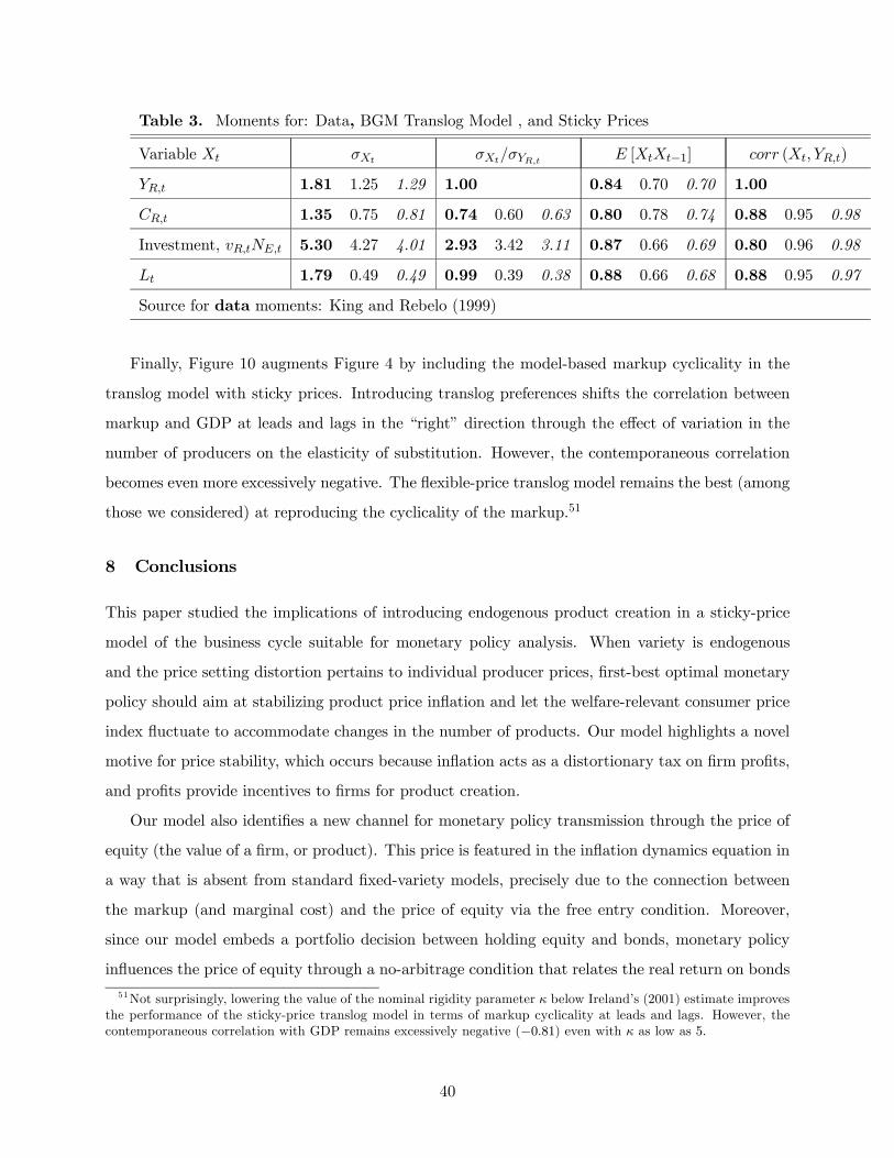
Table 3. Moments for: Data, BGM Translog Model , and Sticky Prices

Variable Xt σXt σXt/σYR,t E [XtXt−1] corr (Xt, YR,t)

YR,t 1.81 1.25 1.29 1.00 0.84 0.70 0.70 1.00

CR,t 1.35 0.75 0.81 0.74 0.60 0.63 0.80 0.78 0.74 0.88 0.95 0.98

Investment, vR,tNE,t 5.30 4.27 4.01 2.93 3.42 3.11 0.87 0.66 0.69 0.80 0.96 0.98

Lt 1.79 0.49 0.49 0.99 0.39 0.38 0.88 0.66 0.68 0.88 0.95 0.97

Source for data moments: King and Rebelo (1999)

Finally, Figure 10 augments Figure 4 by including the model-based markup cyclicality in the

translog model with sticky prices. Introducing translog preferences shifts the correlation between

markup and GDP at leads and lags in the “right” direction through the effect of variation in the

number of producers on the elasticity of substitution. However, the contemporaneous correlation

becomes even more excessively negative. The flexible-price translog model remains the best (among

those we considered) at reproducing the cyclicality of the markup.51

8 Conclusions

This paper studied the implications of introducing endogenous product creation in a sticky-price

model of the business cycle suitable for monetary policy analysis. When variety is endogenous

and the price setting distortion pertains to individual producer prices, first-best optimal monetary

policy should aim at stabilizing product price inflation and let the welfare-relevant consumer price

index fluctuate to accommodate changes in the number of products. Our model highlights a novel

motive for price stability, which occurs because inflation acts as a distortionary tax on firm profits,

and profits provide incentives to firms for product creation.

Our model also identifies a new channel for monetary policy transmission through the price of

equity (the value of a firm, or product). This price is featured in the inflation dynamics equation in

a way that is absent from standard fixed-variety models, precisely due to the connection between

the markup (and marginal cost) and the price of equity via the free entry condition. Moreover,

since our model embeds a portfolio decision between holding equity and bonds, monetary policy

influences the price of equity through a no-arbitrage condition that relates the real return on bonds

51Not surprisingly, lowering the value of the nominal rigidity parameter κ below Ireland’s (2001) estimate improvesthe performance of the sticky-price translog model in terms of markup cyclicality at leads and lags. However, thecontemporaneous correlation with GDP remains excessively negative (−0.81) even with κ as low as 5.

40

(which the central bank influences) to the expected real return on equity. This link between inflation

dynamics and monetary policy through assets prices is central to the validity of the Taylor Principle

in our endogenous-variety model with capital accumulation in the form of new production lines.

This is unlike results from fixed-variety models with physical capital.

Endogenous product variety has implications for inflation dynamics and the estimation of New

Keynesian Phillips curve equations. Empirical proxies for (unobservable) markups need to be

amended in order to estimate Phillips curves in the presence of product creation. Moreover, we

show that the Phillips curve in the presence of endogenous variety features an extra term (with

respect to its fixed-variety counterpart) that depends on the number of available varieties, a state

variable. This goes in the direction of alleviating the notorious difficulty of New Keynesian models

in accounting for inflation persistence with forward-looking price-setting. Finally, we identify an

‘endogeneity bias’ that is present whenever estimates of the Phillips curve ignore product variety

and hence attribute the endogenous component coming from its impact on inflation dynamics to

exogenous ‘cost-push’ shocks.

Numerical exercises show that the sticky-price model performs similarly to the flexible-price

counterpart in terms of matching several features of the U.S. business cycle given a policy spec-

ification that is plausible for inflation-sensitive policymakers. Consistent with the presence of an

endogenous state variable in the Phillips curve, the model generates fairly persistent inflation dy-

namics. These results are confirmed by two extensions of the benchmark setup, studying alternative

assumptions for the initial price setting decision by new entrants and the consequences of non-C.E.S.

(specifically, translog) preferences. Another extension studies a version of the model in which entry

requires purchasing materials rather than hiring labor. In that model, the link between firm value

and marginal production cost implied by free entry disappears: Monetary expansions induce an

increase in entry, but technology shocks generate procyclical markups and immediate deflation for

a wider range of parameter values.

Recent empirical literature has documented the pervasiveness of product creation and destruc-

tion at a frequency that is relevant for business cycle propagation. This paper provides a starting

point for incorporation of this phenomenon in monetary models of the business cycle suitable for

policy analysis. Like the benchmark New Keynesian model with fixed product variety, the bench-

mark model of this paper has shortcomings from an empirical, quantitative perspective. Combined

with the procyclical response of entry to productivity shocks, price stickiness induces excessive

countercyclicality of markups relative to the data. However, the model highlights realistic conse-

41

quences of product creation subject to sunk costs (persistence), a new motive for price stability,

and a new connection between monetary policy and equity prices that is not featured in the pre-

vious New Keynesian literature. The ability of the model to generate procyclical producer entry

and profits (even in the presence of such countercyclical markups) significantly improves on the

New Keynesian benchmark with respect to these stylized facts. Quantitative extensions to address

remaining empirical shortcomings — for instance, the introduction of congestion effects in entry that

would dampen the procyclicality of real wages and the countercyclicality of markups — would be

easy to pursue.52 Thus, we view the model of this paper as a promising stepping stone for future

research on a variety of positive and normative questions in potentially richer, monetary models

with endogenous producer entry.

References

[1] Ambler, S., and E. Cardia (1998): “The Cyclical Behaviour of Wages and Profits under Im-

perfect Competition,” Canadian Journal of Economics 31: 148-164.

[2] Axarloglou, K. (2003): “The Cyclicality of New Product Introductions,” Journal of Business

76: 29-48.

[3] Basu, S., and M. S. Kimball (1997): “Cyclical Productivity with Unobserved Input Variation,”

NBER WP 5915.

[4] Berentsen, A., and C. Waller (2007): “Optimal Stabilization with Endogenous Firm Entry,”

manuscript, University of Basel and University of Notre Dame.

[5] Bergin, P. R., and G. Corsetti (2005): “Towards a Theory of Firm Entry and Stabilization

Policy,” NBER WP 11821.

[6] Bernard, A. B., J. Eaton, J. B. Jensen, and S. Kortum (2003): “Plants and Productivity in

International Trade,” American Economic Review 93: 1268-1290.

[7] Bernard, A. B., S. J. Redding, and P. K. Schott (2006): “Multi-Product Firms and Product

Switching,” NBER WP 12293.

[8] Bilbiie, F. O., F. Ghironi, and M. J. Melitz (2005): “Endogenous Entry, Product Variety, and

Business Cycles,” manuscript, University of Oxford, Boston College, and Princeton University.52Congestion effects would also dampen the positive response of entry to monetary expansions when entry requires

materials.

42

[9] Bilbiie, F. O., F. Ghironi, and M. J. Melitz (2006): “Monopoly Power and Endogenous Va-

riety in Dynamic Stochastic General Equilibrium: Distortions and Remedies,” manuscript,

University of Oxford, Boston College, and Princeton University.

[10] Broda, C. (2004): “CPI Biases and their Impact on Policy”, International Perspectives 32,

Federal Reserve Bank of New York.

[11] Broda, C., and D. E. Weinstein (2006): “Globalization and the Gains from Variety,” Quarterly

Journal of Economics 121: 541-585.

[12] Broda, C., and D. E. Weinstein (2007): “Product Creation and Destruction: Evidence and

Price Implications,” manuscript, University of Chicago and Columbia University.

[13] Calvo, G. A. (1983): “Staggered Prices in a Utility Maximizing Framework,” Journal of Mon-

etary Economics 12: 983-998.

[14] Campbell, J. R. (1998): “Entry, Exit, Embodied Technology, and Business Cycles,” Review of

Economic Dynamics 1: 371-408.

[15] Carlstrom, C. T., and T. S. Fuerst (2005): “Investment and Interest Rate Policy: A Discrete

Time Analysis,” Journal of Economic Theory 123: 4-20.

[16] Chatterjee, S., and R. Cooper (1993): “Entry and Exit, Product Variety and the Business

Cycle,” NBER WP 4562.

[17] Christiano, L. J., M. S. Eichenbaum, and C. L. Evans (1999): “Monetary Policy Shocks: What

Have We Learned and to What End?” in Taylor, J. B., and M. Woodford, eds., Handbook of

Macroeconomics, vol. 1B, 65-148, Elsevier, Amsterdam

[18] Clarida, R., J. Galí, and M. Gertler (1999): “The Science of Monetary Policy: A New Keyne-

sian Perspective,” Journal of Economic Literature 37: 1661-1707.

[19] Clarida, R., J. Galí, and M. Gertler (2000): “Monetary Policy Rules and Macroeconomic

Stability: Evidence and Some Theory,” Quarterly Journal of Economics 115: 147-180.

[20] Comin, D., and M. Gertler (2006): “Medium Term Business Cycles,” American Economic

Review 96: 523-551.

43

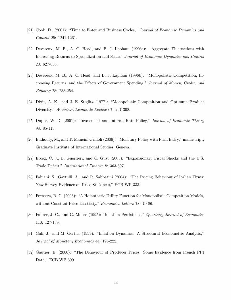
[21] Cook, D., (2001): “Time to Enter and Business Cycles,” Journal of Economic Dynamics and

Control 25: 1241-1261.

[22] Devereux, M. B., A. C. Head, and B. J. Lapham (1996a): “Aggregate Fluctuations with

Increasing Returns to Specialization and Scale,” Journal of Economic Dynamics and Control

20: 627-656.

[23] Devereux, M. B., A. C. Head, and B. J. Lapham (1996b): “Monopolistic Competition, In-

creasing Returns, and the Effects of Government Spending,” Journal of Money, Credit, and

Banking 28: 233-254.

[24] Dixit, A. K., and J. E. Stiglitz (1977): “Monopolistic Competition and Optimum Product

Diversity,” American Economic Review 67: 297-308.

[25] Dupor, W. D. (2001): “Investment and Interest Rate Policy,” Journal of Economic Theory

98: 85-113.

[26] Elkhoury, M., and T. Mancini Griffoli (2006): “Monetary Policy with Firm Entry,” manuscript,

Graduate Institute of International Studies, Geneva.

[27] Erceg, C. J., L. Guerrieri, and C. Gust (2005): “Expansionary Fiscal Shocks and the U.S.

Trade Deficit,” International Finance 8: 363-397.

[28] Fabiani, S., Gattulli, A., and R. Sabbatini (2004): “The Pricing Behaviour of Italian Firms:

New Survey Evidence on Price Stickiness,” ECB WP 333.

[29] Feenstra, R. C. (2003): “A Homothetic Utility Function for Monopolistic Competition Models,

without Constant Price Elasticity,” Economics Letters 78: 79-86.

[30] Fuhrer, J. C., and G. Moore (1995): “Inflation Persistence,” Quarterly Journal of Economics

110: 127-159.

[31] Galí, J., and M. Gertler (1999): “Inflation Dynamics: A Structural Econometric Analysis,”

Journal of Monetary Economics 44: 195-222.

[32] Gautier, E. (2006): “The Behaviour of Producer Prices: Some Evidence from French PPI

Data,” ECB WP 699.

44

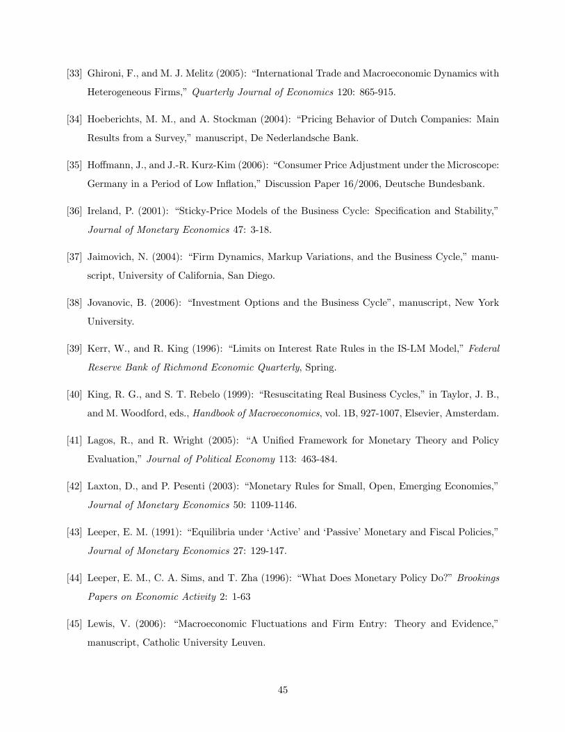
[33] Ghironi, F., and M. J. Melitz (2005): “International Trade and Macroeconomic Dynamics with

Heterogeneous Firms,” Quarterly Journal of Economics 120: 865-915.

[34] Hoeberichts, M. M., and A. Stockman (2004): “Pricing Behavior of Dutch Companies: Main

Results from a Survey,” manuscript, De Nederlandsche Bank.

[35] Hoffmann, J., and J.-R. Kurz-Kim (2006): “Consumer Price Adjustment under the Microscope:

Germany in a Period of Low Inflation,” Discussion Paper 16/2006, Deutsche Bundesbank.

[36] Ireland, P. (2001): “Sticky-Price Models of the Business Cycle: Specification and Stability,”

Journal of Monetary Economics 47: 3-18.

[37] Jaimovich, N. (2004): “Firm Dynamics, Markup Variations, and the Business Cycle,” manu-

script, University of California, San Diego.

[38] Jovanovic, B. (2006): “Investment Options and the Business Cycle”, manuscript, New York

University.

[39] Kerr, W., and R. King (1996): “Limits on Interest Rate Rules in the IS-LM Model,” Federal

Reserve Bank of Richmond Economic Quarterly, Spring.

[40] King, R. G., and S. T. Rebelo (1999): “Resuscitating Real Business Cycles,” in Taylor, J. B.,

and M. Woodford, eds., Handbook of Macroeconomics, vol. 1B, 927-1007, Elsevier, Amsterdam.

[41] Lagos, R., and R. Wright (2005): “A Unified Framework for Monetary Theory and Policy

Evaluation,” Journal of Political Economy 113: 463-484.

[42] Laxton, D., and P. Pesenti (2003): “Monetary Rules for Small, Open, Emerging Economies,”

Journal of Monetary Economics 50: 1109-1146.

[43] Leeper, E. M. (1991): “Equilibria under ‘Active’ and ‘Passive’ Monetary and Fiscal Policies,”

Journal of Monetary Economics 27: 129-147.

[44] Leeper, E. M., C. A. Sims, and T. Zha (1996): “What Does Monetary Policy Do?” Brookings

Papers on Economic Activity 2: 1-63

[45] Lewis, V. (2006): “Macroeconomic Fluctuations and Firm Entry: Theory and Evidence,”

manuscript, Catholic University Leuven.

45

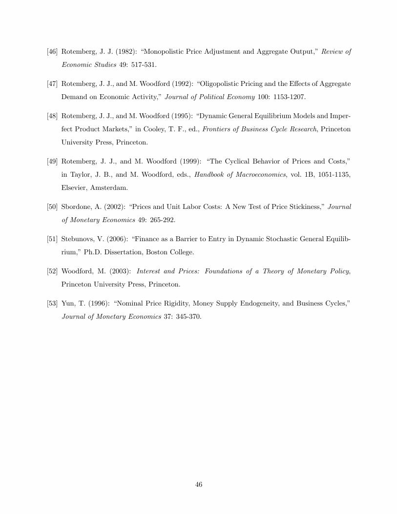
[46] Rotemberg, J. J. (1982): “Monopolistic Price Adjustment and Aggregate Output,” Review of

Economic Studies 49: 517-531.

[47] Rotemberg, J. J., and M. Woodford (1992): “Oligopolistic Pricing and the Effects of Aggregate

Demand on Economic Activity,” Journal of Political Economy 100: 1153-1207.

[48] Rotemberg, J. J., and M. Woodford (1995): “Dynamic General EquilibriumModels and Imper-

fect Product Markets,” in Cooley, T. F., ed., Frontiers of Business Cycle Research, Princeton

University Press, Princeton.

[49] Rotemberg, J. J., and M. Woodford (1999): “The Cyclical Behavior of Prices and Costs,”

in Taylor, J. B., and M. Woodford, eds., Handbook of Macroeconomics, vol. 1B, 1051-1135,

Elsevier, Amsterdam.

[50] Sbordone, A. (2002): “Prices and Unit Labor Costs: A New Test of Price Stickiness,” Journal

of Monetary Economics 49: 265-292.

[51] Stebunovs, V. (2006): “Finance as a Barrier to Entry in Dynamic Stochastic General Equilib-

rium,” Ph.D. Dissertation, Boston College.

[52] Woodford, M. (2003): Interest and Prices: Foundations of a Theory of Monetary Policy,

Princeton University Press, Princeton.

[53] Yun, T. (1996): “Nominal Price Rigidity, Money Supply Endogeneity, and Business Cycles,”

Journal of Monetary Economics 37: 345-370.

46

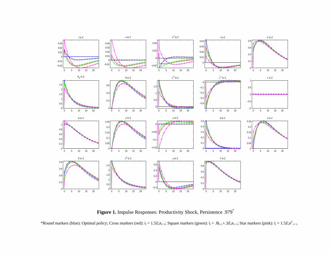
Figure 1. Impulse Responses: Productivity Shock, Persistence .979*

*Round markers (blue): Optimal policy; Cross markers (red): it = 1.5Etπt+1; Square markers (green): it = .8it–1+.3Etπt+1; Star markers (pink): it = 1.5EtπCt+1.

0 5 10 15 20

−0.02

−0.01

0

0.01

0.02

0.03

i to Z

0 5 10 15 20

−0.01

0

0.01

0.02

0.03

0.04

π to Z

0 5 10 15 20

−0.02

0

0.02

0.04

πC to Z

0 5 10 15 20

0

0.01

0.02

0.03

0.04

r to Z

0 5 10 15 200

0.2

0.4

0.6

0.8C to Z

0 5 10 15 200

0.5

1

1.5

2

2.5

NE to Z

0 5 10 15 200

0.2

0.4

0.6

N to Z

0 5 10 15 20

0

0.5

1

1.5

LE to Z

0 5 10 15 20

−0.4

−0.3

−0.2

−0.1

0

LC to Z

0 5 10 15 20−1

−0.5

0

0.5

1L to Z

0 5 10 15 200

0.2

0.4

0.6

0.8

1

w to Z

0 5 10 15 200

0.05

0.1

0.15

0.2

0.25

ρ to Z

0 5 10 15 20−0.15

−0.1

−0.05

0

μ to Z

0 5 10 15 200

0.1

0.2

0.3

0.4

0.5d to Z

0 5 10 15 200

0.05

0.1

0.15

0.2

0.25v to Z

0 5 10 15 200

0.2

0.4

0.6

0.8

D to Z

0 5 10 15 200

0.5

1

1.5

2

2.5

vE to Z

0 5 10 15 20

−0.2

0

0.2

0.4

0.6

y to Z

0 5 10 15 200

0.2

0.4

0.6

0.8

Y to Z

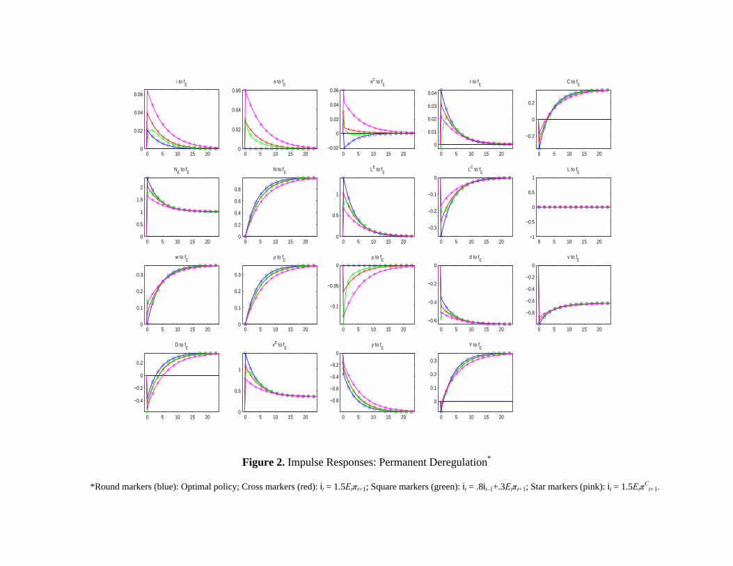
Figure 2. Impulse Responses: Permanent Deregulation*

*Round markers (blue): Optimal policy; Cross markers (red): it = 1.5Etπt+1; Square markers (green): it = .8it–1+.3Etπt+1; Star markers (pink): it = 1.5EtπCt+1.

0 5 10 15 200

0.02

0.04

0.06

i to fE

0 5 10 15 200

0.02

0.04

0.06

π to fE

0 5 10 15 20−0.02

0

0.02

0.04

0.06

πC to fE

0 5 10 15 20

0

0.01

0.02

0.03

0.04

r to fE

0 5 10 15 20

−0.2

0

0.2

C to fE

0 5 10 15 200

0.5

1

1.5

2

NE to f

E

0 5 10 15 200

0.2

0.4

0.6

0.8

N to fE

0 5 10 15 200

0.5

1

LE to fE

0 5 10 15 20

−0.3

−0.2

−0.1

0

LC to fE

0 5 10 15 20−1

−0.5

0

0.5

1

L to fE

0 5 10 15 200

0.1

0.2

0.3

w to fE

0 5 10 15 200

0.1

0.2

0.3

ρ to fE

0 5 10 15 20

−0.1

−0.05

0

μ to fE

0 5 10 15 20

−0.6

−0.4

−0.2

0

d to fE

0 5 10 15 20

−0.8

−0.6

−0.4

−0.2

0

v to fE

0 5 10 15 20

−0.4

−0.2

0

0.2

D to fE

0 5 10 15 200

0.5

1

vE to fE

0 5 10 15 20

−0.8

−0.6

−0.4

−0.2

0

y to fE

0 5 10 15 20

0

0.1

0.2

0.3

Y to fE

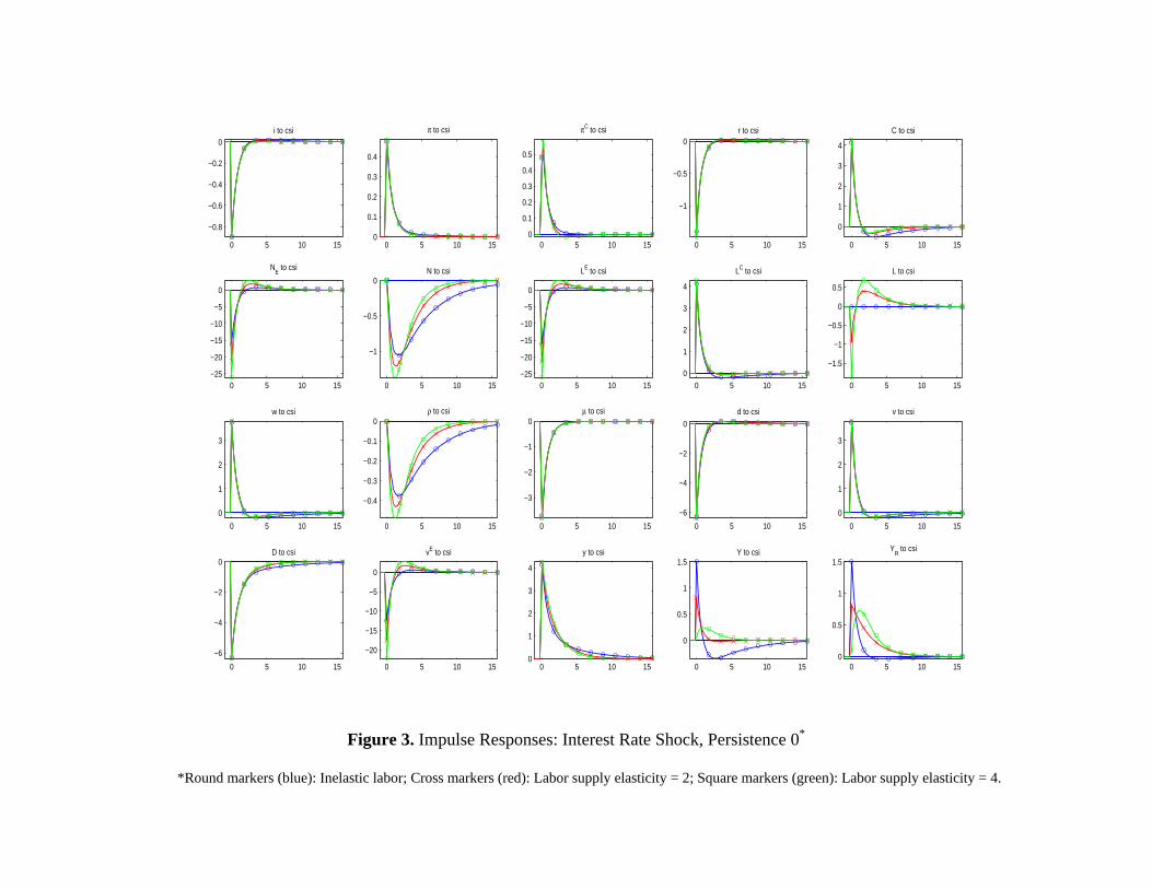
Figure 3. Impulse Responses: Interest Rate Shock, Persistence 0*

*Round markers (blue): Inelastic labor; Cross markers (red): Labor supply elasticity = 2; Square markers (green): Labor supply elasticity = 4.

0 5 10 15

−0.8

−0.6

−0.4

−0.2

0i to csi

0 5 10 150

0.1

0.2

0.3

0.4

π to csi

0 5 10 150

0.1

0.2

0.3

0.4

0.5

πC to csi

0 5 10 15

−1

−0.5

0r to csi

0 5 10 15

0

1

2

3

4

C to csi

0 5 10 15−25

−20

−15

−10

−5

0

NE to csi

0 5 10 15

−1

−0.5

0N to csi

0 5 10 15−25

−20

−15

−10

−5

0

LE to csi

0 5 10 150

1

2

3

4

LC to csi

0 5 10 15

−1.5

−1

−0.5

0

0.5

L to csi

0 5 10 15

0

1

2

3

w to csi

0 5 10 15

−0.4

−0.3

−0.2

−0.1

0ρ to csi

0 5 10 15

−3

−2

−1

0μ to csi

0 5 10 15

−6

−4

−2

0

d to csi

0 5 10 15

0

1

2

3

v to csi

0 5 10 15

−6

−4

−2

0D to csi

0 5 10 15

−20

−15

−10

−5

0

vE to csi

0 5 10 150

1

2

3

4

y to csi

0 5 10 15

0

0.5

1

1.5Y to csi

0 5 10 150

0.5

1

1.5

YR to csi

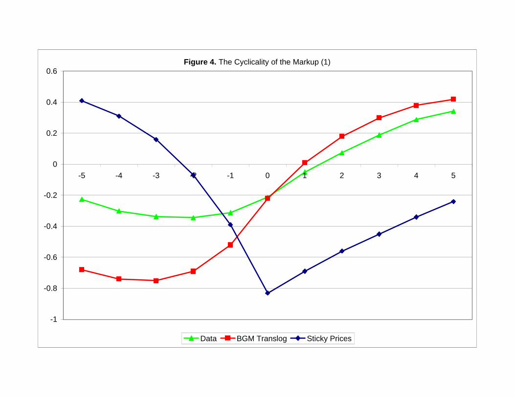
Figure 4. The Cyclicality of the Markup (1)

-1

-0.8

-0.6

-0.4

-0.2

0

0.2

0.4

0.6

-5 -4 -3 -2 -1 0 1 2 3 4 5

Data BGM Translog Sticky Prices

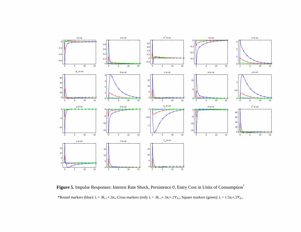
Figure 5. Impulse Responses: Interest Rate Shock, Persistence 0, Entry Cost in Units of Consumption*

*Round markers (blue): it = .8it–1+.3πt; Cross markers (red): it = .8it–1+.3πt+.1YR,t; Square markers (green): it = 1.5πt+.5YR,t.

0 5 10 15

−0.6

−0.4

−0.2

0

i to csi

0 5 10 150

0.2

0.4

0.6

0.8

π to csi

0 5 10 15

−0.2

0

0.2

0.4

0.6

0.8

πC to csi

0 5 10 15

−0.3

−0.2

−0.1

0r to csi

0 5 10 150

1

2

3

C to csi

0 5 10 150

20

40

60

80

NE to csi

0 5 10 150

1

2

3

4N to csi

0 5 10 150

5

10

15

L to csi

0 5 10 150

5

10

w to csi

0 5 10 150

0.5

1

ρ to csi

0 5 10 15

−10

−5

0μ to csi

0 5 10 15

−15

−10

−5

0d to csi

0 5 10 15

−1

−0.5

0

vR to csi

0 5 10 15

−15

−10

−5

0

D to csi

0 5 10 150

20

40

60

80

vE to csi

0 5 10 15

0

5

10

15

y to csi

0 5 10 150

5

10

15

Y to csi

0 5 10 150

5

10

15

YR to csi

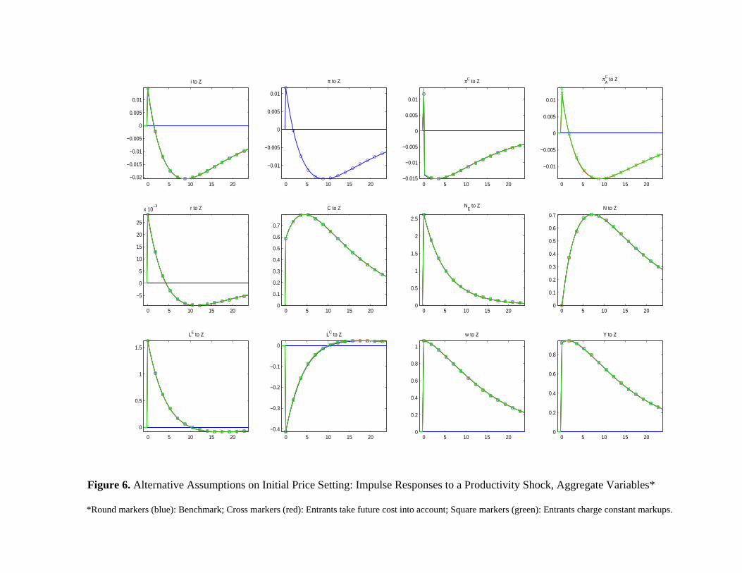
Figure 6. Alternative Assumptions on Initial Price Setting: Impulse Responses to a Productivity Shock, Aggregate Variables*

*Round markers (blue): Benchmark; Cross markers (red): Entrants take future cost into account; Square markers (green): Entrants charge constant markups.

0 5 10 15 20−0.02

−0.015

−0.01

−0.005

0

0.005

0.01

i to Z

0 5 10 15 20

−0.01

−0.005

0

0.005

0.01

π to Z

0 5 10 15 20−0.015

−0.01

−0.005

0

0.005

0.01

πC to Z

0 5 10 15 20

−0.01

−0.005

0

0.005

0.01

πCA to Z

0 5 10 15 20

−5

0

5

10

15

20

25

x 10−3 r to Z

0 5 10 15 200

0.1

0.2

0.3

0.4

0.5

0.6

0.7

C to Z

0 5 10 15 200

0.5

1

1.5

2

2.5

NE to Z

0 5 10 15 200

0.1

0.2

0.3

0.4

0.5

0.6

0.7N to Z

0 5 10 15 20

0

0.5

1

1.5

LE to Z

0 5 10 15 20−0.4

−0.3

−0.2

−0.1

0

LC to Z

0 5 10 15 200

0.2

0.4

0.6

0.8

1

w to Z

0 5 10 15 200

0.2

0.4

0.6

0.8

Y to Z

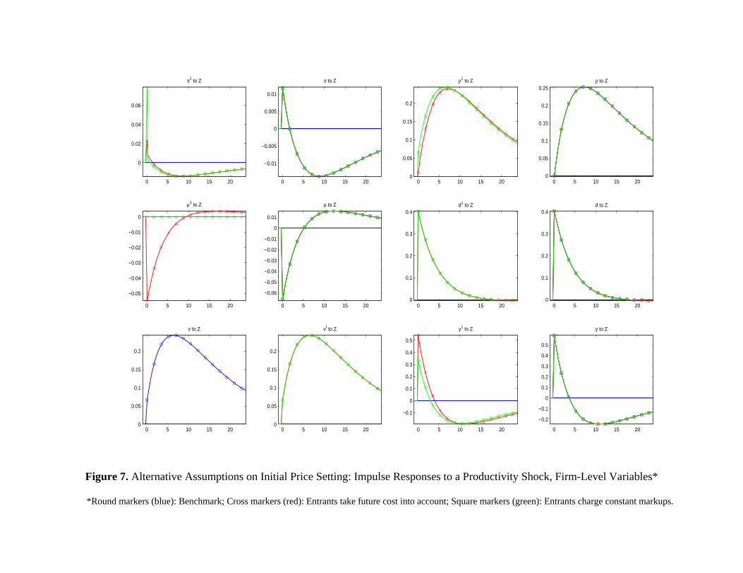
Figure 7. Alternative Assumptions on Initial Price Setting: Impulse Responses to a Productivity Shock, Firm-Level Variables*

*Round markers (blue): Benchmark; Cross markers (red): Entrants take future cost into account; Square markers (green): Entrants charge constant markups.

0 5 10 15 20

0

0.02

0.04

0.06

π1 to Z

0 5 10 15 20

−0.01

−0.005

0

0.005

0.01

π to Z

0 5 10 15 200

0.05

0.1

0.15

0.2

ρ1 to Z

0 5 10 15 200

0.05

0.1

0.15

0.2

0.25ρ to Z

0 5 10 15 20

−0.05

−0.04

−0.03

−0.02

−0.01

0

μ1 to Z

0 5 10 15 20

−0.06

−0.05

−0.04

−0.03

−0.02

−0.01

0

0.01

μ to Z

0 5 10 15 200

0.1

0.2

0.3

0.4d1 to Z

0 5 10 15 200

0.1

0.2

0.3

0.4d to Z

0 5 10 15 200

0.05

0.1

0.15

0.2

v to Z

0 5 10 15 200

0.05

0.1

0.15

0.2

vt to Z

0 5 10 15 20

−0.1

0

0.1

0.2

0.3

0.4

0.5

y1 to Z

0 5 10 15 20

−0.2

−0.1

0

0.1

0.2

0.3

0.4

0.5

y to Z

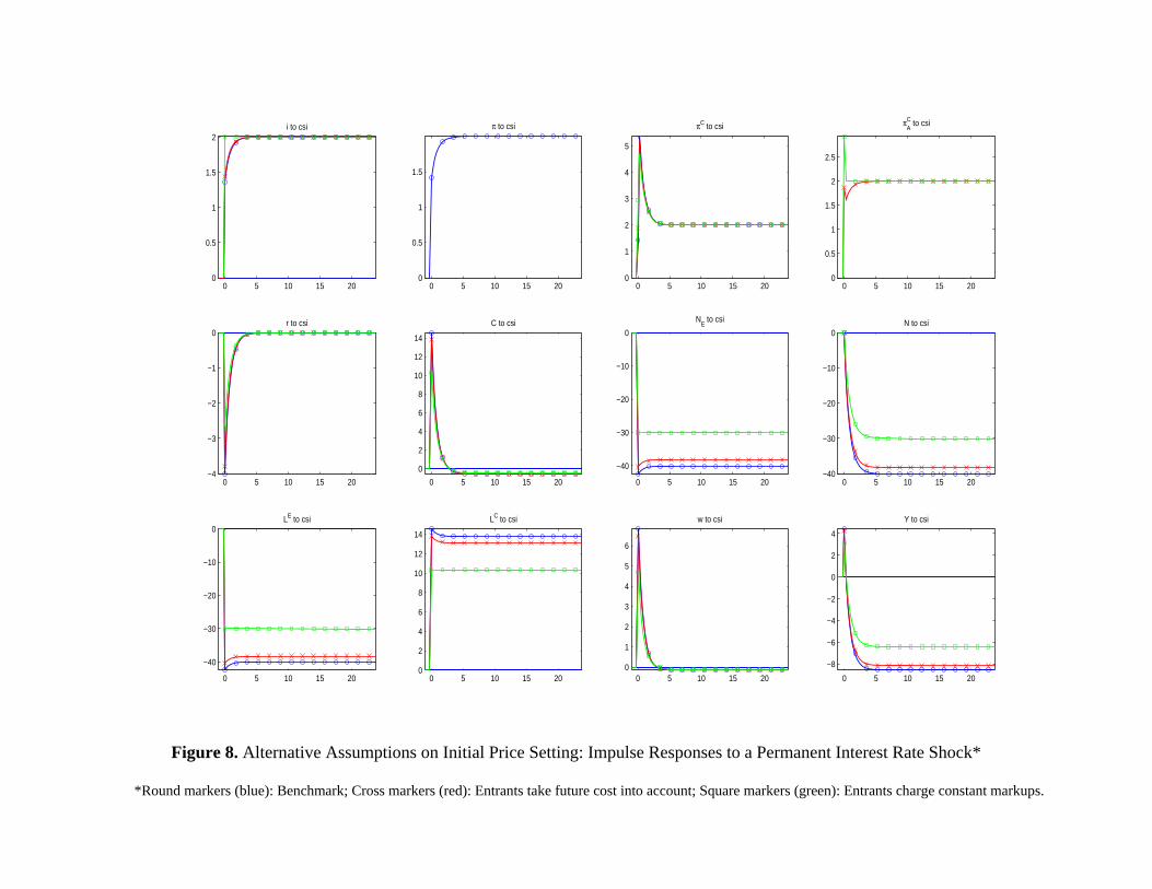
Figure 8. Alternative Assumptions on Initial Price Setting: Impulse Responses to a Permanent Interest Rate Shock*

*Round markers (blue): Benchmark; Cross markers (red): Entrants take future cost into account; Square markers (green): Entrants charge constant markups.

0 5 10 15 200

0.5

1

1.5

2i to csi

0 5 10 15 200

0.5

1

1.5

π to csi

0 5 10 15 200

1

2

3

4

5

πC to csi

0 5 10 15 200

0.5

1

1.5

2

2.5

πCA to csi

0 5 10 15 20−4

−3

−2

−1

0r to csi

0 5 10 15 20

0

2

4

6

8

10

12

14

C to csi

0 5 10 15 20

−40

−30

−20

−10

0

NE to csi

0 5 10 15 20−40

−30

−20

−10

0N to csi

0 5 10 15 20

−40

−30

−20

−10

0LE to csi

0 5 10 15 200

2

4

6

8

10

12

14

LC to csi

0 5 10 15 200

1

2

3

4

5

6

w to csi

0 5 10 15 20

−8

−6

−4

−2

0

2

4

Y to csi

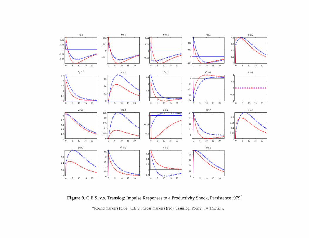
Figure 9. C.E.S. v.s. Translog: Impulse Responses to a Productivity Shock, Persistence .979*

*Round markers (blue): C.E.S.; Cross markers (red): Translog; Policy: it = 1.5Etπt+1.

0 5 10 15 20

−0.02

−0.01

0

0.01

0.02

i to Z

0 5 10 15 20

−0.01

0

0.01

0.02π to Z

0 5 10 15 20

−0.01

0

0.01

0.02πC to Z

0 5 10 15 20−0.01

0

0.01

0.02

r to Z

0 5 10 15 200

0.2

0.4

0.6

0.8C to Z

0 5 10 15 200

0.5

1

1.5

2

2.5

NE to Z

0 5 10 15 200

0.2

0.4

0.6

N to Z

0 5 10 15 20

0

0.5

1

1.5

LE to Z

0 5 10 15 20−0.4

−0.3

−0.2

−0.1

0

LC to Z

0 5 10 15 20−1

−0.5

0

0.5

1L to Z

0 5 10 15 200

0.2

0.4

0.6

0.8

1

w to Z

0 5 10 15 200

0.05

0.1

0.15

0.2

0.25ρ to Z

0 5 10 15 20

−0.1

−0.05

0

μ to Z

0 5 10 15 20

0

0.1

0.2

0.3

0.4d to Z

0 5 10 15 200

0.05

0.1

0.15

0.2

v to Z

0 5 10 15 200

0.2

0.4

0.6

D to Z

0 5 10 15 200

0.5

1

1.5

2

2.5

vE to Z

0 5 10 15 20

−0.2

0

0.2

0.4

0.6

y to Z

0 5 10 15 200

0.2

0.4

0.6

0.8

Y to Z

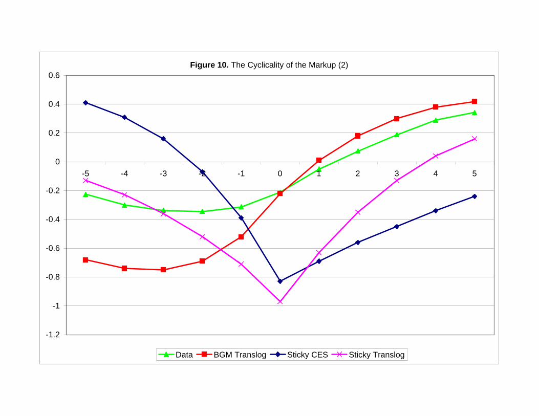
Figure 10. The Cyclicality of the Markup (2)

-1.2

-1

-0.8

-0.6

-0.4

-0.2

0

0.2

0.4

0.6

-5 -4 -3 -2 -1 0 1 2 3 4 5

Data BGM Translog Sticky CES Sticky Translog