MONETARY INTERVENTION MITIGATED BANKINGPANICS DURING THE GREAT DEPRESSION? QUASI-EXPERIMENTAL

EVIDENCE FROM THE FEDERAL RESERVE DISTRICTBORDER IN MISSISSIPPI, 1929 TO 1933

Gary Richardson

William Troost

WORKING PAPER 12591

NBER WORKING PAPER SERIES

MONETARY INTERVENTION MITIGATED BANKING PANICS DURING THEGREAT DEPRESSION: QUASI-EXPERIMENTAL EVIDENCE FROM THE FEDERAL

RESERVE DISTRICT BORDER IN MISSISSIPPI, 1929 TO 1933

Gary RichardsonWilliam Troost

Working Paper 12591http://www.nber.org/papers/w12591

NATIONAL BUREAU OF ECONOMIC RESEARCH1050 Massachusetts Avenue

Cambridge, MA 02138October 2006

We thank friends and colleagues for advice and encouragement. Dan Bogart, Michael Bordo, Jan Brueckner,Ami Glazer, Michelle Garfinkel, Jean-Laurent Rosenthal, Eugene White, and participants in seminarsat the Federal Deposit Insurance Corporation, Federal Reserve Board of Governors, NBER SummerInstitute, Rutgers University, UC Irvine, and Western Economics Association provided commentson earlier drafts. Please direct inquiries to the principal author, Gary Richardson, garyr@uci.edu. Theviews expressed herein are those of the author(s) and do not necessarily reflect the views of the NationalBureau of Economic Research.

© 2006 by Gary Richardson and William Troost. All rights reserved. Short sections of text, not toexceed two paragraphs, may be quoted without explicit permission provided that full credit, including© notice, is given to the source.

Monetary Intervention Mitigated Banking Panics During the Great Depression: Quasi-ExperimentalEvidence from the Federal Reserve District Border in Mississippi, 1929 to 1933Gary Richardson and William TroostNBER Working Paper No. 12591October 2006JEL No. E5,E6,E65,N1,N2

ABSTRACT

The Federal Reserve Act of 1913 divided Mississippi between the 6th (Atlanta) and 8th (St. Louis)Federal Reserve Districts. Before and during the Great Depression, these districts' policies differed.The Atlanta Fed championed monetary activism and the extension of credit to troubled banks. TheSt. Louis Fed adhered to the doctrine of real bills and eschewed expansionary initiatives. Outcomesdiffered across districts. In the 6th District, banks failed at lower rates than in the 8th District, particularlyduring the banking panic in the fall of 1930. The pattern suggests that discount lending reduced failurerates during periods of panic. Historical evidence and statistical analysis corroborates this conclusion.

Gary RichardsonDepartment of EconomicsUniversity of California, IrvineIrvine, CA 92697-5100and NBERgaryr@uci.edu

William TroostDepartment of Economics University of California, IrvineIrvine, CA 92697-5100wtroost@uci.edu

1

Banks failed throughout the Great Depression. Their demise contributed to the disruption of

financial intermediation, contraction of monetary aggregates, and decline in aggregate demand that

spawned the deepest downturn in American history (Benjamin Bernanke, 1983; Milton Friedman and

Anna Schwartz, 1963; Christina Romer, 1993; Peter Temin, 1989). The Federal Reserve did little to

stem the falling tide. It failed for many reasons. Its leaders adhered to outdated doctrines and

monitored misleading indicators of monetary conditions. The Board of Governors lacked leadership

and could not coordinate policies amongst its disputatious districts. The gold standard fettered

mechanisms of monetary policy (Barry Eichengreen, 1992).

Even if the Federal Reserve had tried to alleviate the banking crisis, no clear evidence exists that it

could have helped depository institutions. Two schools of thought exist on this issue. One school believes

the principal causes of banking crises were withdrawals of deposits, illiquidity of assets, and the Federal

Reserve’s reluctance to act. The Fed could have alleviated banking problems by acting as a lender of last

resort (Friedman and Schwartz, 1963; Elmus Wicker, 1996). The second school concludes that banks

failed because the economy contracted. Asset prices fell. Loan default rates rose. Banks became insolvent,

continuing a process of liquidation and consolidation in the banking industry that began during the 1920s.

In such circumstances, the Fed could not aid banks by injecting liquidity into the banking system (Temin,

1976; Charles Calomiris and Joseph Mason, 2003).

These opposing views coexist for several reasons. One is methodological. None of the studies

directly measures the effects of monetary policy. All infer the Fed’s ability to influence the banking

system indirectly, by analyzing correlations between bank failures and economic activity which in theory

should shed light on the issue. Another reason the debate continues is differences in data sources.

Friedman and Schwartz (1963) analyze data on bank suspensions aggregated at the national level. Their

successors scrutinize similar series at lower levels of aggregation, or disaggregated data consisting of

samples of national banks, or panels of banks from within individual cities, states, or Federal Reserve

districts. The most recent and comprehensive work analyzes a panel of data for all Federal Reserve

member banks. Future research, Calomiris and Mason (2003, p. 1639) indicate, should analyze data on all

banks, multiple measures of financial distress such as suspensions and liquidations, and multiple channels

of contagion such as bank runs and correspondent linkages.

Even with such data, analyzing the impact of Federal Reserve policies would be difficult. At the

national level, Fed policies were endogenous reactions to ongoing economic events. Changes in Fed

policies often coincided with changes in fiscal, tariff, and regulatory policies and with shocks to the

economy for which data is insufficient or nonexistent. At the district level, the boundaries of Federal

2

Reserve Districts coincided in most cases with state borders. States changed policies throughout the

depression, often at the same time and occasionally in reaction to actions of the Federal Reserve.

Economic shocks also differed across states. The endogeneity of policies, simultaneous changes in

multiple policy dimensions, and the spectrum of unobserved impede efforts to attribute differences in

outcomes to differences in policies. When observed, correlations between outcomes and policies might

have been caused by phenomena for which investigators cannot control.

In such circumstances, quasi-experimental econometric strategies have become increasingly

popular. The task is to find a group of banks that operated in a single regulatory and economic

environment but which were exposed to different Federal Reserve policy regimes. Comparing outcomes

across regimes yields insights free from problems of inference inherent in traditional analysis. The

obvious place to seek such a group is along the Federal Reserve district borders. Borders occasionally

divided states. Mississippi is an example. Its northern half lay within the 8th Federal Reserve District (St.

Louis). Its southern half lay within the 6th Federal Reserve District (Atlanta). The two districts’ policies

differed dramatically early in the depression. St. Louis was a staunch advocate of non-intervention.

Atlanta was a leading advocate of assisting banks in need. The St. Louis and Atlanta Feds applied their

different policies to the portions of Mississippi lying within their jurisdictions. The adoption of these

policies preceded the onset of the depression, and had little to do with circumstances in Mississippi,

which was a small and peripheral portion of each Federal Reserve district, and much to do with the

philosophies and experiences of the leadership of the two banks. Thus, the application of Federal Reserve

policies to Mississippi possessed the characteristics of an exogenous policy experiment.1

This essay analyzes the impact of Federal Reserve policies in the Mississippi case. Section 1

describes the data that we analyze. Section 2 examines the historical and economic justification for

1 Mississippi possesses advantages over all other candidates for quasi-experimental analysis. The principal proponents of

monetary activism were the 2nd (New York) and 6th (Atlanta) districts. They shared within-state borders with the 8th (St. Louis), 3rd (Philadephia), and 1st (Boston) districts, which at the onset of the depression adhered to the doctrine of real bills. The 6th/8th district border divided Mississippi along a line of latitude into regions of equal size with similar industrial, agricultural, and demographic environments. In contrast, the 6th/8th district border in Tennessee separated regions with distinct industries and agricultures and which experienced different shocks during the downturn. The collapse of Caldwell and Company, which initiated the first banking panic of the depression, occurred in the 6th District’s section of the state. Similar concerns complicate analysis along the borders of the 2nd district. The 1st/2nd district border in Connecticut and the 2nd/3rd district border in New Jersey separated the commercial and industrial suburbs of New York City from the rest of each state. It may be difficult to determine whether differences in outcomes along those borders were due to Federal Reserve policies or New York City effects. In addition, the unit-banking system in Mississippi was widely representative of the type of banks which failed in large numbers during the early 1930s, and as the last section of this essay discusses, the small-to-medium sized banks which predominated in Mississippi were the type which throughout the nation played the largest role in transmitting financial panics, depositors’ behavior, and monetary policy to the real economy. The experience of banks in New York (state, city, and metropolitan area), where failure rates were low and uncorrelated across time and institutions, was not representative of banks in the rest of the nation.

3

employing quasi-experimental methods. Section 3 describes our methods and results. Our analysis

progresses through two stages. The first is a non-parametric examination of the building blocks of

duration analysis: survival and hazard functions. The second is a parametric analysis of our panel of data.

These methods directly address key questions concerning the collapse of the banking system during the

early 1930s. Did Federal Reserve policies influence bank failure rates? Did monetary intervention

mitigate banking panics? Did providing liquidity (or credibly committing to do so) reduce rates of bank

suspension and liquidation? To each question, the answer is yes.

Our statistical methods indicate that inter-district differences in discount lending generated

interdistrict differences in survival rates during banking panics. No other factor observed in our panel data

set does so. Section 4 examines the robustness of this result, and eliminates plausible alternative

explanations of the patterns that appear in the data. Principle alternatives include shocks, selection, and

policies that might have occurred but which in our panel data set, we do not observe. This section presents

an array of qualitative, quantitative, and analytical evidence pertaining to those possibilities. This

additional data demonstrates that these phenomena could not have caused banks in the 6th District to

survive during the banking panic in the fall of 1930 at higher rates than banks in the 8th District. In most

cases, these phenomena were ‘unobserved’ because they did not, in actuality, occur.

Section 5 discusses the implications of our analysis. By injecting liquidity into the banking

system, particularly during the banking panic in the fall of 1930, the Federal Reserve Bank of Atlanta

reduced bank failure rates. If other Federal Reserve Banks had pursued similar strategies, fewer banks

would have failed, and the course of the depression may have been different.

1. Data Sources

The extant evidence is insufficient for the investigation of events in Mississippi. No published data

distinguishes banks lacking liquidity from banks suffering insolvency or banks that suspended payments

temporarily from those which closed permanently. No scholarly study elucidates the policies pursued by

the Federal Reserve Bank of Atlanta. No scholarly study describes the banking panics which struck

Mississippi. The Biennial Report of the Banking Department of the State of Mississippi lacks information

on individual operating banks.

An array of sources, however, provides the essential information. The Rand McNally Bankers’

Directory describes individual banks. Details include balance sheet data, correspondents, Federal Reserve

membership, and dozens of other bank characteristics. Rand McNally published biennially in July and

January. Information for Mississippi state banks appears to have been updated in June annually.

4

Observations drawn from the July issue, therefore, provide a panel of annual observations on state and

national banks at their spring calls. Table 1 and 2 recapitulate this information. The former indicates the

number of banks in operation during the depression. The latter presents summary statistics for individual

bank characteristics.

Data on economic conditions comes from several sources. The United States Censuses of

Agriculture, Manufacturing, and Population provide data on the characteristics of counties. Summary

statistics appear in Table 3. Bradstreet’s Weekly, Dun’s Review, The Commercial and Financial

Chronicle, the Federal Reserve Bulletin, and the Annual Reports of the Federal Reserve Board and the

Federal Reserve Banks provide information on building permits, business failures, commodity prices,

interests rates, and price and production indices.

The archives of the Federal Reserve Board of Governors provide additional information. The

Division of Bank Operations form St. 6386b reports individual bank suspensions and their causes. Form

St. 6386c reports changes in bank status such as reopenings of suspended institutions and voluntary

liquidations, a category of closures in which banks ceased operations and arranged to repay depositors the

full value of their deposits without the intervention of courts or receivers.2 This data distinguishes

between temporary and permanent closures of banks. A temporary suspension occurred when a bank

closed its doors to the public for the opening of at least one business day, whether or not the bank

reopened for business at some time in the future. Permanent liquidations were the subset of suspensions

where insolvent banks permanently ceased operations, surrendered charters, sold assets, and repaid

creditors to the greatest extent possibly usually under the auspices of a court appointed officer called a

receiver.

From these sources, we construct a data panel consisting of all banks that operated in Mississippi

between July 1929 and July 1933. Our panel contains standard information about bank characteristics and

economic conditions and novel information such as multiple measures of financial distress (including

suspensions and liquidations), all other possible changes in bank status (including mergers, consolidations

forced by financial difficulties, and voluntary liquidations), multiple paths of contagion (including

correspondent linkages and runs on banks), factors fundamental to the performance of the national

economy and particularly pertinent to Mississippi (such as levels of farm indebtedness and the condition

of the cotton crop), and measures of Federal Reserve policy regimes.

To determine the policy regimes of the Atlanta and St. Louis Federal Reserve Banks, we examine 2 These records reside in Record Group 82, Central Subject File of the Federal Reserve Board of Governors, 1913-1954,

National Archives and Records Administration, College Park, Maryland. For detailed descriptions of this archival evidence, see Richardson (2004 and 2006).

5

a wide variety of historical sources. The archives of the Board of Governors contain correspondence

between the Board, the Atlanta Fed, and the St. Louis Fed which describes the actions and illuminates the

intentions of the two districts. So does Richard Gamble’s in-house history of the Atlanta Fed (1989) and

articles in depression-era newspapers and periodicals. The monthly bulletins and annual reports of the

Reserve Banks also describe their policies and provide data demonstrating the implementation of their

plans. Additional evidence of implementation comes from the weekly balance sheets of each Reserve

Bank and Banking and Monetary Statistics (Board of Governors, 1943).

Three independent sources enable us to determine the dates and the nature of Mississippi’s

banking crises. The first source is data collected by the Board of Governors’ Division of Bank Operations

on Form St. 6386b, which indicates the causes of bank suspensions. The second source is the narrative

description of events contained within the biennial reports of Mississippi’s state banking department. The

third is articles in seven newspapers including three of the most prominent in Mississippi, the Meridian

Star, Vicksburg Herald, and Vicksburg Sunday Post-Herald; the leadings papers from the headquarters’

cities of the 6th and 8th Federal Reserve Districts, the Atlanta Journal, St. Louis Globe-Democrat, and St.

Louis Post-Dispatch; and the New York Times.

2. Historical Background

Our quasi-experimental approach builds upon three facts. First, when the depression began, the

policy regimes of Atlanta and St. Louis Federal Reserve Banks differed, and those differences were

exogenous to the state of Mississippi and events occurring at the time. In the summer of 1931, the St.

Louis Fed reformulated its policy regime, and thereafter, its actions resembled those of the Atlanta Fed.

Second, in Mississippi, bank suspensions surged on two occasions, and the nature of those surges

differed. During the panic which began in December 1930, depositors withdrew funds from all banks en

masse. During the crises in the fall of 1931 and winter of 1933, depositors withdrew funds from some, but

not all, banks after shocks to fundamentals temporarily confused depositors about the solvency of

depository institutions. Third, Mississippi was economically homogenous, particularly in counties

adjacent to the Federal Reserve district boundary.

2.1 Policy Regimes of 6th and 8th Districts

Friedman and Schwartz (1963) pioneered efforts to identify Federal Reserve policy regimes by

analyzing historical documents. Scholars who have followed in their footsteps have named their method

the narrative historical approach. Principal proponents of the method, Christina and David Romer,

emphasize the importance of establishing clear criteria for identifying policy regimes, particularly during

6

the interwar era, when there was wide “variation in monetary institutions, in the theoretical framework

adhered to by central bankers, and in the particulars of important monetary episodes (C. Romer and D.

Romer, 1989).” Since our essay focuses on bank failures, we define policy regimes in terms of a Federal

Reserve district’s philosophies, plans, and rules regarding the extension of aid to troubled banks and

concerning whether and how to intervene during banking panics. In our case, the identification of these

regimes is simplified by the stability of the leadership of the 6th and 8th Federal Reserve Districts from the

founding of the Federal Reserve until the reorganization of the system during the Roosevelt

Administration.

In the spring of 1913, the organizing committee of the Federal Reserve System split the state of

Mississippi into nearly equal portions. Counties lying north of 33 degrees latitude became a part of the 8th

District. Counties lying south of that line became a part of the 6th District. Banks located in one district

could petition to be placed under the jurisdiction of different districts. A few banks in central Louisiana

took this opportunity to shift from the 8th to the 6th District, after it established a branch in New Orleans.

However, no banks in Mississippi requested a transfer in either direction (Gamble, 1989, p. 5).

Since its inception, the Federal Reserve Bank of Atlanta pursued a policy similar to

Bagehot’s Law, a doctrine that during financial panics, central banks should act as lenders of last

resort and extend credit to all financial institutions, and if necessary, to merchants and firms. Such

lending should be substantial enough to enable solvent but illiquid banks to survive deposit losses

and the contraction of credit, and thus, to prevents runs from driving healthy banks into insolvency.3

Prior to the stock market crash in October 1929, the Atlanta Fed faced four situations when it

could employ such policies. In 1920, a cotton price bubble burst, triggering financial panics

throughout the South. In 1926, rumors triggered runs on banks in Cuba, where the Atlanta Fed

operated a branch office. In the spring of 1929, an infestation of Mediterranean fruit flies crippled

crops in central Florida, triggering runs on banks in Tampa which threatened to spread throughout

the state. In September 1929, bank runs once again swept Cuba. In each instance, the Atlanta Fed

rushed large quantities of cash to the afflicted region, extended emergency loans to member banks,

helped member banks extend credit to their country clients, and returned the situation to status-quo

ex-ante.

During the twelve months following the stock market crash in October 1929, rates of bank failure

3 Bagehot’s Law is named after Walter Bagehot, one of its earliest and most influential advocates. His classic explication of

the doctrine appears in Lombard Street (Bagehot 1873). In the canonical version of Bagehot’s Law, the lender of last resort charges a penalty rate, to discourage banks from relying on such assistance and to alleviate moral hazard. During the Great Depression, the Atlanta Fed did not charge a penalty rate.

7

resembled those that had prevailed throughout the previous decade. In November 1930, however,

Caldwell and Company failed in Nashville, Tennessee. The firm controlled one of the largest banking

chains in the South, and its principal affiliates, the Bank of Tennessee, held deposits from hundreds of

institutions. When reports of the incident reached Atlanta, the Governor of the Federal Reserve Bank of

Atlanta, Eugene Black, and two cashiers rushed to the scene to help the Federal Reserve branch in

Nashville supply currency and credit to banks in the city and surrounding region. Two days later, runs

began on banks in Knoxville. Deposits in each of the three largest institutions, the Holston-Union Bank,

City National Bank, and the East Tennessee National Bank, fell by $500,000 in an afternoon, forcing the

banks to invoke the thirty day clause on certificate holders and savings depositors. One of Atlanta’s

cashiers rushed to Knoxville, while Eugene Black endeavored “to aid the Knoxville situation in any way

that [he] could” and “keep the Nashville situation in check.” In a report to the board on November 14,

Black wrote that

We are shipping sums to these two banks [City National and East Tennessee National] in Knoxville which will be adequate for any demand made upon them and I am hopeful that the situation there has been relieved (Gamble, 1989, p. 20).

Caldwell’s collapse had repercussions throughout the surrounding region. Suspension rates rose rapidly in

states, such as Arkansas, with banking chains linked to the Caldwell conglomerate.

As the 6th District endured the onslaught following Caldwell’s collapse, it acted everywhere as it

had in the past. It rushed cash in large quantities to banks undergoing runs. It extended credit to member

banks as quickly and substantially as possible and helped them extend loans to their correspondents and

clients. During the first three weeks of the Caldwell crisis, discounts to member banks increased by

$2,800,000. Total Federal Reserve credit outstanding increased by more than $8,100,000 (Wicker, 1996,

p. 54).

At the nadir of the depression in late 1932 and early 1933, the Atlanta Fed repeated this

performance, and advanced funds to “member banks on any asset having value (Gamble, 1989, pp. 22-

23).” At that time, as they had throughout the contraction, the leaders of the Federal Reserve Bank of

Atlanta advocated expansionary doctrines. The Governors of the Atlanta and New York Federal Reserve

Banks, Eugene Black and George Harrison, “were the only Reserve Bank governors who advocated

significant open-market purchases during the depression (Wheelock, 1991, p. 97; see also Meltzer 2003 p.

293).” Black’s insistent advocacy of expansionary initiatives eventually won the ear of Congress and the

President, who appointed Black chairman of the Federal Reserve Board of Governors in 1933.

The policies and philosophies of the Federal Reserve Bank of St. Louis were far different. During

the panic following the collapse of Caldwell, the St. Louis Fed did not rush to extend loans and may have

8

slowed their disbursement by more stringently monitoring the quality of paper submitted for

rediscounting. During the first three weeks of the crisis, discounts to member banks in the 8th District

declined by $2,100,000. Total Federal Reserve credit outstanding in the 8th District declined by more than

$11,800,000 (Wicker, 1996, p. 54). The St. Louis bank was one of only three Reserve banks – including

Chicago and Cleveland – which “thought that discount rates should be held above market rates (Caroline

Whitney, 1934, p. 68).”

The St. Louis Fed’s reluctance to extend credit to banks or increase the monetary base, either

through open-market purchases or the discount window, “stemmed from a fundamental Real Bills view

that the supply of credit should contract during recessions” since a lower level of economic activity

required less credit to sustain it (Wheelock, 1991, pp. 53, 111). According to this doctrine, occasional

depressions weeded out inefficient firms, moderated wages, and cleansed the capitalist system. Excessive

credit expansion generated fears of inflation and uncertainty about interest rates which deterred business

investment and retarded economic activity. For this reason, the directors “opposed reductions in discount

rates and other actions [which would] retard the necessary process of liquidation (Lester Chandler, 1971,

p. 142).” The St. Louis Fed retained this hard line position throughout the first 18 months of the

depression.

Attitudes changed, however, during the summer of 1931. In July, the St. Louis Fed ceased to

oppose intervention and eased restrictions on discount lending. The 8th District’s chairman wrote that

open-market purchases of government securities “may have been of some benefit. Therefore, it seems to

me worthwhile to continue the experiment (Chander 1971 p. 142).” In the spring of 1932, the St. Louis

Fed participated in the open-market purchase program pursued by the Federal Reserve System as a whole.

The operation of the discount window appears to have been a principal difference between the 6th

and 8th Districts. The Federal Reserve Act of 1913 narrowly defined assets that banks could use as

collateral when borrowing from the Federal Reserve. Legal changes expanded this authority. The Glass-

Steagall Act (February 27, 1932) permitted Federal Reserve Banks to discount hitherto ineligible assets

for member banks. The Emergency Relief and Construction Act (July 21, 1932) allowed Federal Reserve

banks to lend money to “individuals, partnerships, and corporations” having no other sources of funds

(Whitney, 1934, p. 64). The Emergency Banking Act (March 9, 1933) empowered Federal Reserve banks

“under exceptional and exigent circumstances … to make advances to member banks which have no

eligible assets on their own promissory notes secured to the satisfaction of the Reserve Bank (Whitney,

1934, p. 65).”

The Federal Reserve Act permitted, but did not require, Reserve Banks to discount eligible paper.

9

Reserve Banks possessed broad discretion about when, to whom, and under what condition to extend

loans. During the 1930s, Reserve Banks exercised this discretion and regulated borrowing by individual

member banks directly, rather than relying on the discount rate to ration loans (Anderson, 1965, p. 47).

Reserve Banks closely monitored member bank borrowing. Most Reserve Banks used a basic line,

sometimes seasonally adjusted, to determine which member banks borrowed excessively. Reserve Banks

discouraged the use of discounts either to supplement a member bank’s own resources or to take

advantage of rate differentials. Member banks that persisted in such activities found the discount window

closed to them (Anderson, 1965, pp. 46-47). The Board of Governors encouraged such practices. In 1929,

the Board of Governors “directed the Reserve Banks to pursue a policy of ‘direct pressure,’ in which

discount loans simply were refused to any bank carrying stock market loans (Wheelock, 1991, p. 73).” In

1931, when applications at discount windows mounted at a record rate, the Federal Reserve sent member

banks a letter admonishing them for such behavior and stressing the inappropriateness of increased bank

borrowing (Lloyd Thomas, 2005, p. 389).

The operative aspect of discount window operations were, therefore, the willingness of Federal

Reserve Banks to extend loans based on various forms of collateral. Throughout the depression, the

Federal Reserve Bank of Atlanta operated an open window. It extended loans to member banks that

wanted to borrow at the prevailing rate and, up until February 1932, possessed sufficient eligible paper,

and after February 1932, possessed assets of any type judged to be of any value. During panics, the

Federal Reserve Bank of Atlanta rushed funds to afflicted areas, sent personnel to expedite the lending

process, and publicly proclaimed its willingness to extend credit sufficient to alleviate the situation. This

behavior constituted Atlanta’s policy regime, which remained constant throughout the depression.

St. Louis Fed’s policy regime changed in midstream. Until the summer of 1931, the Federal

Reserve Bank of St. Louis adhered to the doctrine of real bills and its prescription of pro-cyclical policies.

It ran a tight discount window. It took little or no action to expedite the lending process during periods of

panic. It limited lending and frequently refused requests to rediscount eligible paper. When it did extend

loans, the St. Louis Fed usually required what was then known as marginal or double collateral – that is,

collateral consisting of the eligible paper required by law plus an equal amount of United States

government securities, which remained as collateral on deposit at the Fed until the loan was repaid. This

practice discouraged banks from using the discount window as a source of liquidity, since they had to

pledge $2 of their most liquid assets to get $1 of cash (Westerfield 1932). In the summer of 1931, the St.

Louis Fed changed policies, eased collateral requirements, and expanded lending through the discount

window. Thereafter, its philosophies and policies moved towards those of the Federal Reserve Bank of

10

Atlanta.

Data on discounting in Table 4 illuminates differences between the districts. At the end of 1929,

Atlanta extended credit to member banks principally by rediscounting commercial paper. St. Louis

extended credit principally upon the security of United States government obligations. At the end of 1933,

after the Glass-Steagall Act of 1932 expanded the discretionary lending powers of the Federal Reserve

district banks, commercial paper remained over 60% of Atlanta’s discounts. Hitherto ineligible assets

amounted to more than one-quarter of Atlanta’s total lending. In St. Louis, the majority of lending to

member banks continued to be secured by United States government obligations. About one-tenth of all

lending was on hitherto ineligible assets.

Figures 1 and 2 illuminates changes in discount lending during the crises in the falls of 1930 and

1931. After the collapse of Caldwell, discounts of the 6th District rose rapidly, peaking at a level more

than 40% higher than that before the crisis. Discounts of the 8th District fell gradually, as the extension of

new discount loans slowed and existing discount loans expired. After Britain abandoned the gold standard,

both the 6th and 8th Districts raised discount rates substantially and restricted lending. Discounts of the 6th

District plunged nearly 50% in two weeks. Discounts of the 8th District declined steadily. Three months

later, discounts of both districts converged to a new level, roughly 25% lower than the previous level.

The last issue concerning Federal Reserve policy is how it affected non-member institutions. The

preponderance of banks in Mississippi did not belong to the Federal Reserve System and could not

directly access the Federal Reserve discount window. They could, however, discount eligible paper

through and borrow funds from banking correspondents. All non-member institutions possessed

correspondents which cleared checks, processed wire transfers, and provided other services that linked

non-member institution to the wider financial system. Non-member institutions kept deposits at

correspondent banks in reserve cities, and these deposits counted as a portion of the non-member’s legal

reserves. Non-members needing liquidity turned to their correspondents. The Federal Reserve encouraged

(or discouraged) correspondents from providing liquidity by promising to loan (or withhold loans) from

them in turn. In other words, the Federal Reserve controlled the liquidity of non-member institutions by

influencing the willingness and ability of correspondents to extend credit.

2.2 Banking Crises

Bank failures occurred most often in Mississippi during two periods when bank failure rates rose

in other states. Scholars identify two events as triggers (not necessarily exclusive) of these surges in bank

suspensions.

First, on 7 November 1930, Caldwell and Company collapsed. Failures initially spread through

11

correspondent networks to banks in Tennessee, Arkansas, Illinois, and North Carolina. Caldwell’s

correspondent network did not extend into Mississippi, where the banking situation remained calm for six

weeks following Caldwell’s collapse. Newspapers in Mississippi, however, reported the financial scandal

underlying Caldwell’s demise (e.g. Vicksburg Herald, Saturday, 8 November 1930, p. 1). The scandal

remained a prominent news item for the next two months. Newspapers also covered defalcations of

greater magnitude which caused the closure of the Guaranty Building and Loan Association and affiliated

investment institutions in Hollywood, California (Atlanta Journal, 12 December 1930, pp. 1, 10) and the

closure of the Bank of the United States in New York City (Atlanta Journal, 11 December 1930, p. 33; 12

December 1930, p. 36; 16 December 1930, p. 29). Mississippi’s newspapers also emphasized a court

decision that invalidated a law which exempted state banks from taxation (Meridian Star, 1 December

1930, p. 1). The decision threatened to increase banks’ operating expenses and weaken their financial

position. The decision also cast doubt upon the states recently revised banking codes and threatened to

saddle operating banks with large liabilities from the deposit insurance program which the state

discontinued in the spring.

The incessant discussion of financial corruption, banking panics, industrial recession, and court

cases appears to have taken a toll on depositors’ confidence. The Vicksburg Herald’s weekly tabulation of

Vicksburg bank balance sheets shows deposits falling at a rapid and increasing rate during November and

December. The process remained orderly until Friday, December 19, 1930, when panic struck. On that

day, the state banking department closed three banks; one due to embezzlement, and two due to frozen

assets and poor collections. The next day, one of the larger banks in the state “placed itself in the hands of

the State Banking Department for liquidation because of an unusual situation caused by the death of G. A.

Wilson (Atlanta Journal, 21 December 1930, p. 11).”

Rumors triggered runs on nearby banks, which soon spread to neighboring towns, and within a

week, throughout the state. Bank funs forced the closure of 49 institutions. Other institutions suspended

operations to forestall runs which management believed to be imminent. State law allowed banks to close

their doors to depositors for up to five days and for a longer period if they could demonstrate both

compelling necessity and the ability to reopen after the crisis passed. Banks that remained in operation

slowed the decline in deposits by restricting withdrawals from savings accounts for periods of up to 30

days (a provision in most deposit contracts) and refusing to terminate time deposits ahead of the maturity

date. The number of bank runs fell during January. Runs occurred sporadically in February. The last bank

to suspend operations due to deposit losses did so on March 2, 1931.

During this whirlwind of withdrawals, aggregate deposits at Mississippi’s banks fell by more than

12

40%, and they remained at this lower level for the remainder of the depression. During the same period,

banks liquidated roughly one-third of their assets. “The amount of paper held by the banks in the form of

loans and discounts reached its low figure at the end of the year 1930 (Mississippi Banking Department,

1931, p. 4).” Resources remained near this nadir for the next two years. From the peak in 1929 to the

trough in 1933, total deposits in Mississippi’s banks declined by 55.1%.

Mississippi’s second surge in bank suspensions began after England abandoned the gold standard

on 11 September 1931. Britain’s action did not directly affect banks in Mississippi, which lacked links to

financial centers abroad. Fear that the United States might also abandon the gold standard, however,

reduced deposits at banks in American money centers. To combat the external drain and defend the gold

standard, the Federal Reserve System raised discount rates from 1.5% to 3.5% in two steps in October

1931, reduced the monetary base, and restricted discount lending. These actions weakened the financial

position of banks throughout the nation.

In Mississippi, depositors withdrew substantial sums from some banks. The afflicted institutions

tended to be in poor financial condition. A few of the banks which closed their doors due to deposit losses

managed to reopen, but most of them did so only after recapitalizing, either through assessments on

stockholders, contributions by depositors, or both. The first failure due to deposit losses occurred on

November 13, 1931. The last occurred on January 11, 1932. During this episode, aggregate deposits at

banks in Mississippi changed little, and “no liquidation of consequence” occurred in terms of bank assets

(Mississippi Banking Department, 1931, p. 4).”

In sum, the historical record reveals two banking crises in Mississippi. The first, in December

1930, was a panic of the type modeled by Diamond-Dybvig (1983), in which a sudden shift in depositors’

perceptions about the safety and solvency of the financial system triggered runs on banks. Withdrawals en

masse forced banks to liquidate assets, or to suspend operations temporarily, or to seek assistance from

lenders of last resort. Solvent institutions which could not maintain cash flows suspended operations

temporarily. Solvent institutions which could not bear the costs of such actions went out of business. The

second, in the fall 1931, was a crisis of the type modeled by Jacklin and Battacharya (1988), where

adverse shocks pushed some banks into insolvency. Depositors did not know which banks would fail and

withdrew funds from banks whose health they questioned.

2.3 Economic Conditions

Mississippi was homogenous in regulatory, economic, and demographic dimensions. Mississippi’s

banking department applied standard procedures throughout the state. So did departments of federal

government, since Mississippi lay within a single district for the Office of the Comptroller of Currency,

13

Reconstruction Finance Corporation, Department of Agriculture, Works Progress Administration, and all

other organizations which we have checked. Mississippi’s economic and demographic structures were

similar throughout the state. Table 3 demonstrates this by displaying county-level data drawn from the

censuses of population, manufacturing, and agriculture for 1930. The columns segregate the information

by Federal Reserve district. In both the 6th and 8th Districts, the fraction of the population in the labor

force was substantial. Unemployment rates were low. Levels of farm debt hovered around one-third to

one-fifth of farm value. Rural counties concentrated on cultivating cotton, with cotton farms comprising

nearly 80% of the acres in the northern half of the state and 60% of the acres in the southern section.

Disposable incomes differed little across counties. Prevailing prices for labor (average annual

manufacturing wage in row (5)) and capital (ratio of interest charges to mortgage debt in row (13)) also

differed little across counties. The largest differences arose in the extremities of the state. The

southernmost counties abutting the Gulf of Mexico retained large swaths of undeveloped bayou and

substantial maritime industries. The counties adjoining the Federal Reserve district border had few

discernible differences.

2.4 The Historical Experiment

The homogeneity of banking systems and business conditions and the exogeneity of policies

makes Mississippi’s experience a valid policy experiment. The homogeneity of treatment groups and

exogeneity of treatments implies that differences in outcomes resulted from differences in treatments.

What differences should be expected? During the post-Caldwell panic, when the Atlanta Fed

followed Bagehot’s Law and the St. Louis Fed followed the doctrine of real bills, economic theory

predicts that bank failure rates in the 6th District should have been lower than bank failure rates in the 8th

District. In the Diamond-Dybvig framework, which characterizes this panic, a lender of last resort can

mitigate a financial panic by extending credit to illiquid institutions (and perhaps forestall a panic by

credibly committing to do so). Liquidity enables financial institutions to satisfy the demands of depositors

without unloading assets at panic prices. Since the Atlanta Fed implemented such a policy in a prompt,

ample, and public manner, difference in outcomes between the 6th and 8th Districts (if any) should reveal

the effectiveness (or ineffectiveness) of Atlanta’s policies.

In contrast, during the crisis in the fall of 1931, when the Atlanta and St. Louis Fed pursued

similar contractionary policies, the 6th and 8th Districts should have experienced similar suspension and

14

liquidation rates.4 Economic theory strengthens this prediction. In the Jacklin-Battacharaya framework,

which characterizes that event, real shocks and imperfect information are the fatal factors. Withdrawals,

which reallocate funds from questionable to healthy banks, threaten a few banks on the margin. A lender

of last resort may be able to aid those marginal institutions, but it cannot change the fate of insolvent

banks. Since illiquidity is not the root of the problem, creating liquidity cannot solve the problem.

Non-panic periods serve as a control case which helps to test the homogeneity assumption

underlying our analysis. Bagehot’s Law is a policy implemented during panics, when withdrawals,

contagion, and illiquidity bedevil banks. The policy does not operate, and therefore, should have no direct

effect on bank failure rates outside of panic periods.5

2.5 Basic Patterns in the Data

Table 5 and Figure 3 illuminate the patterns of bank failures at the heart of this essay. Table 5

reports suspension and liquidation rates for each year from July 1929 to July 1934. The rates peaked in

the second year of the depression and remained above pre-depression levels until the national banking

holiday in March, 1933. Table 5 shows that when the Atlanta and St. Louis Feds pursued opposite

policies during the fall and winter of 1930, fewer banks failed in the 6th District, which made every effort

to inject liquidity into the banking system. More banks failed in the 8th District, which preached non-

intervention and where Federal Reserve credit outstanding fell substantially. Afterward, as the policies of

the districts converged and the nature of the banking difficulties changed, rates of suspension and

liquidations did likewise. For the entire contractionary phase of the Great Depression, July 1929 through

March 1933, the rate of suspension in the 8th District (59.2%) exceeded the rate in the 6th District (38.7%)

by a wide margin. The rate of liquidation in the 8th District (34.4%) exceeded the rate in the 6th District

(26.8%) by a smaller amount.

Figure 3 illustrates these patterns by plotting the percentage of banks in business and operation

each day over the entire span of our data panel from 1 July 1929 to 30 June 1933. Figure 3 also indicates

the date when the St. Louis Fed’s policies began to converge toward those of the Atlanta Fed and the

dates of the events which the historical literature identifies as triggers of the surges in suspensions

apparent in the evidence. Figure 3 shows that during the post-Caldwell panic, when policy regimes

4 In the lexicon of experimental analysis, the fall of 1931 serves as a placebo treatment. The experimental and control groups

receive similar therapies, and therefore, should experience similar outcomes. If outcomes differ, some unnoted difference between the groups must be influencing the results, and the experimental design may be invalid.

5 In this sentence, the caveat ‘direct’ indicates that Bagehotian policies might influence outcomes in non-panic periods indirectly, either by (a) influencing bankers’ expectations of the probabilities and consequences of future panics, and thereby, influencing bankers’ behavior, or (b) altering the composition of banks that survive panics. The former might alter behavior and outcomes in pre-panic periods. The latter might alter outcomes in post panic periods.

15

differed across districts, banks suspended operations (temporarily and permanently) at much higher rates

in the 8th District. During later banking crises, when policies differed little and the rise in failures

stemmed largely from fundamental factors, banks in the 6th and 8th Districts failed at similar rates.

3. Methods and Results

Statistical analysis substantiates this supposition by controlling for characteristics of individual

banks, the economic environment, and other phenomena which might have generated the observed

differences across districts. Section 3.1 controls for potentially confounding factors non-parametrically.

Section 3.2 presents parametric estimates.

3.1 Non-Parametric Estimates

The analysis of time-to-failure rests on survivor and hazard functions. This section presents non-

parametric estimates of survivor functions constructed via the Kaplan-Meier method and of hazard

functions constructed by smoothing raw hazard rates (i.e. the number of bank failures divided by the

number of banks at risk on each date). Kernels are Epanechnikov. Bandwidths of 28 days on graphs

spanning four years and 7 days on graphs spanning four months are wide enough to smooth daily

volatility without obscuring weekly shifts in the probability of failure.

Figure 4 presents survival and hazard functions for all banks in Mississippi during the three

banking crises. In Figure 4(a) and (b), the time under analysis is restricted to the four months following

the collapse of Caldwell and Company. In Figure 4(c) and (d), the time under analysis is the four months

after Britain abandoned the gold standard. In each figure, the population at risk is all banks in operation. A

bank that surrendered its charter voluntarily or merged with another institution departs from the

population at risk (but is not counted as a failure) on the date when it ceased operations. A bank that

suspended operations is counted as a failure on the date that it closed its doors to the public.

In Figure 4, the gray lines depict the 6th District. The black lines depict the 8th District. Figures 4(a)

and (b) show that following Caldwell’s collapse, patterns of hazard and survival differed dramatically

between the 6th and 8th Districts. Failure rates in the 8th District rose rapidly and exceeded those in the 6th

District for most of the crisis. The array of standard non-parametric tests for the equality of survival

functions – including the log rank, Breslow, Peto-Peto, and Tarone-Ware tests – reject at the 1%

significance level the null hypothesis of that the survival function for the 6th District equaled that for the

8th District. All of the tests produce χ2 statistics (with 1 degree of freedom) of over 20.

Figures 4(c) and (d) show that after Britain abandoned the gold standard, suspension rates in the

6th District resembled those in the 8th District. For a brief period in November, suspensions occurred more

16

frequently in the southern half of the state, but hazard rates soon rose north of the border. Tests of equality

of the survivor functions cannot reject the null hypothesis of equality. The standard tests all produce χ2

statistics of less than 1.

Figure 5 demonstrates that differences in suspension rates across districts during the post-Caldwell

panic cannot be attributed to fundamentals or selection. Figures 5(a) and (b) limit the analysis to banks

that operated within one degree latitude of the Federal Reserve district border.6 Figures 5(c) and (d) limit

the analysis to banks operating within 50 miles of the border. These figures demonstrate that even in a

narrow band along the border, banks failed at a higher rate in the 8th District and a lower rate in the 6th

District. Economic fundamentals varied little over such short distances, particularly in economically and

politically homogenous central Mississippi. Thus, differences in fundamentals were not the reason that

failure rates differed between districts.

Figures 5(e) and (f) limit the analysis to banks in operation before the founding of the Federal

Reserve in 1913. Figures 5(g) and (h) limit the analysis to banks founded after the Federal Reserve

System. These figures demonstrate that banks in both groups failed at a higher rate in the 8th District.

Therefore, selective pressures, which would have altered the pattern for one of these groups, were not the

reason that failure rates differed between districts.

Table 6 extends the comparative exercise of the Figure 5 to later periods of panic. The table

indicates the results of log-rank tests for the equality of survival functions from the 6th and 8th Districts.

The test statistics are χ2 with 1 degree of freedom. For the post-Caldwell panic, the null hypothesis of

equality can be rejected in every instance. For the post-Britain-abandoned-gold and post-Roosevelt-

election surges in suspensions, the null hypothesis of equality cannot be rejected.

Figure 6 illustrates patterns of suspensions over the entire sample period. The event under analysis

is suspension of operations. The definition of the population at risk remains as above except for

temporarily suspended banks, which depart the population at risk when suspended and reenter the

population at risk after resuming operations. All of the graphs depict a similar pattern. In the 8th District,

more banks failed, and failures were clustered during periods of panic. In the 6th District, fewer banks

failed, particularly during the banking panic of 1930, and failures were spaced more evenly through time.

6 Throughout this essay, whenever we state ‘within 1º latitude of the border,’ we are referring to this county-based distance

definition. The set includes all banks operating within a county for which at least 50% of the surface area of the county lay within one degree latitude of the border. This geographic restriction defines a band running through the center of the state straddling the Federal Reserve district border. The outer edges of the band vary from 70 to 95 miles distance from the boundary. This county-based measure of distance from the border proves useful in regressions whose explanatory variables include county-level characteristics, county fixed effects, or county contagion effects as well as error terms clustered by county.

17

Figures 6(a) and (b) illuminate important issues. During non-panic periods, the suspension rate in

the 6th District exceeded that of the 8th District, particularly in the period preceding the collapse of

Caldwell, when principal employers in two towns in the southern half of the state closed, forcing nearby

banks out of business. This pattern suggests that economic fundamentals favored banks in the 8th District

over those in the 6th District. During periods of panic, however, banks in the 8th District failed at higher

rates. This pattern is consistent with the effective application of Bagehot’s law, which should reduce

liquidation rates during panics, when the lender of last resort loans freely, but not during normal times,

when the lender of last resort husbands its reserves and allows insolvent banks to liquidate.

The remaining figures demonstrate the robustness of the result. Figures 6(c) and (d) limit the

analysis to all banks that operated within one degree latitude of the border. Figure 6(e) and (f) limit the

analysis to all banks that operated within 50 miles of the border.7 Figures 6(g) and (h) limit the analysis to

banks established before 1913. The pattern remains the same. The pattern also remains the same when we

limit analysis to groups of banks with similar characteristics, such as longevity or stable management, or

groups of banks operating in similar environments, such as cities or cotton-growing regions.

Subpopulations which we have examined include state banks, non-member banks, member banks,

national banks, banks in the western and eastern halves of the state, banks in operation for more or less

years than the median age of all banks, banks with and without management changes between 1925 and

1929, banks in counties with more and less than the median percentage of agricultural acreage dedicated

to cotton cultivation, and banks in counties with above and below the median number of manufacturing

establishments. A companion essay available from the authors shows that when the measure of distress is

changed to liquidation, patterns of survival and hazard do not change. For both suspensions and

liquidations, our results also hold for all subpopulations which we have examined. The invariance of the

pattern across subpopulations defined by likely correlates with economic fundamentals and selected

characteristics suggests that neither fundamentals nor selection drive our results.

The tripartite pattern apparent in Figure 6 – (1) hazard rates for the 6th and 8th Districts similar at

all times except during panic following Caldwell’s collapse, when the hazard for the 8th District exceeded

that in the 6th by a wide margin, (2) cumulative hazard for the entire period higher in the 8th District, (3)

failures clustered during three periods of heightened risk – appears robust to reasonable alterations in our

non-parametric framework. A non-parametric test for this pattern, however, does not exist. Generating

such tests requires additional assumptions. For this task, we turn to parametric methods.

7 Note: The pattern persists even for extremely small bands. For example, in a 25 mile radius around the border, 8 banks

failed in the 8th district, while only one bank failed in the 6th district.

18

3.2 Parametric Estimates

A plethora of potential parameterizations exist for our analysis. We present results for the current

gold standard in this literature, the log-logistic survival model of Calomiris and Mason (2003b). In this

model, the unit of observation is the individual bank. The dependent variable is log days until liquidation.

Time under observation begins on July 1, 1929 and ends at the national banking holiday in March 1933.

The explanatory variables include the characteristics of banks, the characteristics of counties in which

banks operate, measures of business conditions at the state and national level, indicators of periods of

panic, and in our version of this model, indicators of Federal Reserve policy regimes. Bank characteristics

update annually each July 1st. County characteristics (from Census of 1930) remain constant over time.

National and state economic conditions update monthly. This framework allows us to determine the

relative importance of fundamentals and contagion as sources of bank distress and to test whether Federal

Reserve intervention mitigated (or accentuated) banking panics.

Table 7 presents the results of this exercise. Column (1) reports the basic model. It contains

indicator variables for the three banking crises, for whether a bank operated within the 6th District, and for

whether during each of three banking crises a bank operated within the 6th District. The crisis indicators

reveal to what extent liquidation rates rose above the baseline during each period of panic. These

crisis/district interaction terms reveal for each crisis whether liquidation rates differed between the 6th and

8th Districts. The coefficient for the fall 1930 crisis indicator is statistically significant, indicating that

during the crisis, the liquidation rate rose above the baseline. The coefficient for fall ’30 crisis/Atlanta Fed

interaction term is also statistically significant, indicating that during the crisis, banks in the 6th District

liquidated at lower rates than banks in the 8th District. We cannot reject the null hypothesis that the other

coefficients equal zero, suggesting that during the later crises, outcomes differed little from the baseline or

between Federal Reserve districts.

Table 8 reveals the magnitudes of the coefficients. Column (1) indicates the crisis in the fall of

1930 raised bank liquidation rates substantially. The marginal effects can be stated as changes in

cumulative hazard rates (a metric readily comparable to that of the graphs in the previous section). The

regression coefficients, the parametric assumptions concerning the survival function, and the data can be

combined to estimate the probability of liquidation for each bank for each day during the crisis period.

The mean estimate is 1.593 per thousand. A counterfactual – what would the hazard rate have been in the

absence of the panic – can be estimated by setting the panic indicator variable equal to zero and redoing

the calculation. The mean estimate for the counterfactual is 0.089 per thousand. The average difference in

estimates is 1.504 per thousand. Compounding over the 73 days of the fall ’30 crisis reveals that the panic

19

increased the cumulative hazard for each bank by 11.0%. The fall ’30 crisis, in other words, accounts for

approximately one third of the total cumulative hazard experienced by banks in Mississippi between July

1929 and March 1933. Similar calculations reveal the effect of the Atlanta Fed’s expansionary policy

during the fall ’30 crisis. Cumulative hazard in the 6th District was 10.2% lower than cumulative hazard in

the 8th District. In other words, in the 8th District, where the St. Louis Fed followed the real bills doctrine,

the crisis in the fall of 1930 raised cumulative hazard by 11.0%, while in the 6th District, where the

Atlanta Fed followed Bagehot’s Law, the crisis increased cumulative hazard by only 0.8%.

Columns (2) through (6) in Tables 7 and 8 strengthen this supposition. Column (2) adds to the

explanatory variables a vector of bank characteristics. The characteristics include the percentage of total

assets comprised of cash, exchanges with banks, and marketable securities [Assets % Cash]; net worth as

a share of total assets [Net Worth / Total Assets]; deposits as a percentage of total liabilities [Liabilities %

Deposits]; the number of years that the bank had been in operation; whether the bank possessed a state

charter; the natural log of total assets; and the percentage of non-cash assets invested in real estate. We do

not report coefficients for the latter two variables, which are statistically insignificant in most

specifications.8

In all of our specifications, we correct standard errors for heterogeneity using the Huber-White

sandwich method with error terms clustered on individual banks. We account for the possibility of

selective survival based on unobserved characteristics using the standard frailty method of assuming a

gamma distribution for the unobserved parameters and estimating the parameter (theta) of that distribution.

While these corrections improve the efficiency of our estimates, in no case do they change the signs or

significance levels of the key coefficients.

Columns (3) and (4) add to the regression the characteristics of the counties within which each

bank operated. Column (3) adds measures of population density, the ratio of aggregate farm debt to farm

value, the percentage of land under cultivation planted with cotton, the percentage of farm acres in pasture

or fallow, and the percentage of farms under 100 acres. This set of five county characteristics is the most

powerful, parsimonious specification which we have identified among the hundreds of available county-

level characteristics. Rather than accounting for county characteristics by choosing a subset of the

numerous, available variables, Column (4) adds to the regression the 12 principal components (as

8 Note: Our database contains over 30 bank characteristics. We chose to include these seven because they have clear

interpretations. For example, Assets % Cash indicates liquidity. Net Worth indicates solvency. Liabilities % Deposits indicates the cost of capital and vulnerability to changes in depositors’ preferences for cash. In addition, these seven provide the most powerful, parsimonious set of explanatory variables. Results obtained with them correspond closely to results obtained from running regressions on the principal components of the array of all bank characteristics.

20

identified by the Kaiser Criterion) of the vast array of county-level data. Employing the principal

components improves the fit of our regression, but changes neither the signs nor the significance levels of

variables concerning the banking crises and Federal Reserve policy regimes, and changes their

magnitudes only marginally.

Column (5) adds variables measuring temporal variation in state and national economic conditions.

The variables are the dollar values of building permits in Mississippi as well as the value of building

permits and business bankruptcies for the United States as a whole. The variables enter the regression in

the form which maximizes the value of their coefficients and minimizes the value of the coefficients for

the banking panics and policy regimes. Building permits (for both Mississippi and the United States) enter

the regressions in an annual log difference transformation at lags of 3 and 5 months. Business failures

enter the regression in contemporaneous levels. Incorporating this information improves the fit of our

regression, increases the estimated magnitude of the impact of the banking crisis and monetary

intervention in the fall of 1930 (see Table 8, column (5)), but reduces the precision of the estimate (see

Table 7, column (5)).

Column (6) estimates the canonical Calomiris and Mason version of the model. We format our

data as in their (2003b) essay, employing identical county, state, and national data and nearly identical

bank characteristics, and replicate their result. The regression does an excellent job of predicting the

longevity of individual institutions. Fundamentals are highly correlated with bank distress. However, our

version of the model includes indicators for Federal Reserve policy regimes. The coefficients on these

indicators demonstrate that the Federal Reserve could lower bank failure rates by acting as a lender of last

resort during banking panics.

Our model of fundamentals enables us to perform an additional exercise. Split the banks into two

groups, those operating in the 6th District and those operating in the 8th District. For each group, use a

parsimonious probit model of bank and county characteristics in July 1929 to predict suspension rates

between July 1929 and June 1930. Then, use the coefficients from that regression and characteristics in

July 1930 to predict suspension rates between July 1930 and June 1931.

Table 9 presents the results. Column (i) indicates the average predicted probability of suspension

for 1929. Column (iii) indicates the actual suspension rate in 1929. The null hypothesis that the former

equals the latter cannot be rejected, demonstrating that our model fits the data reasonably well. Column

(ii) indicates the average predicted probability of suspension for 1930. The prediction for the 8th District

changes little, because the balance sheets of banks in the 8th District changed little between July 1929 and

July 1930. The prediction for the 6th District falls substantially, because the 6th Districts high failure rate

21

for 1929 was driven by adverse shocks in particular counties. In 1930, fewer banks operate in those

counties (in fact, almost all of the banks in those counties failed). In the remainder of the district, the

balance sheets of banks, and thus the predicted probability of failure, changed little. Comparing Columns

(ii) and (iv) shows that our model of fundamentals which fit the data well for 1929 does not predict the

events that occurred in the following year.

A more complicated model, where we define insolvency and illiquidity thresholds, and run a

multinomial logistic regression predicting suspensions, liquidations, consolidations, and voluntary

departures from the banking business, yields the same conclusions. The relationship between

fundamentals and failures changes radically between the first and second years of the depression. During

the first year of the depression, fundamentals were worse and failure rates were higher in the 6th District.

During the second year of the depression, fundamentals remained much as they had before. The banks

operating in the two districts appear to have been in similar financial shape and to have had similar

prospects of survival. The increase in failure rates following Caldwell’s collapse (and the different fates

faced by the two districts) was not a product of the fundamental forces acting on the banking system in

the recent past.

4. Robustness, Shocks, Selection, Alternative Explanations, and Additional Evidence

Our conclusion remains robust to a wide variety of alterations in our econometric framework.

Models employing different parametric assumptions, explanatory variables, and corrections for

heterogeneity and serial correlation yield identical qualitative and similar quantitative results. The

robustness of our results suggest that the specifications which we report successfully control for

differences in the observed characteristics of banks and the environments in which they operate. All of

our parametric regressions also include corrections for unobserved heterogeneity and selection on

unobserved characteristics. Our non-parametric analysis demonstrates that our results do not depend upon

particular mathematical and statistical assumptions.

As we noted earlier, differences between districts in economic conditions, bank characteristics,

and government policies violate the homogeneity assumption underlying our analysis. The design of our

study, which limits analysis to a single state, and the statistical tests which we perform in the preceding

section, allay this concern, at least for the observable characteristics of the environment and institutions.

We have also tried to correct for unobserved characteristics, as much as possible given the statistical

methods available.

Several crucial issues, however, cannot be addressed statistically. Could some unmeasured

22

fundamental shock explain differences between the 6th and 8th Districts during the post-Caldwell crisis?

To be consistent with the evidence, the shock would have to be one which raised failure rates in the 8th

District relative to the 6th District during the period beginning December 19, 1930 and ending March 2,

1931, but neither before nor after, and the shock would have to be one which affected the districts

uniformly and which retained its punch right up to the border, but which did not spill over into the

adjoining district. The shock could not be one which we have controlled for both parametrically and non-

parametrically. Such shocks include anything correlated with the characteristics of banks – such as size,

age, services, financial characteristics, or Federal Reserve membership – or the economic or demographic

characteristics of the towns or counties in which banks operated – such as population density, number of

manufacturing establishments, and cotton cultivation. These facts seem to rule out all possible climatic,

cultural, agricultural, and industrial shocks, all of which would seem to be correlated with our controls or

to operate on time-horizons longer than ten weeks.

Could the confounding factor be financial links to the Caldwell conglomerate or geographic

proximity to the locus of the post-Caldwell panic? The evidence indicates otherwise. Consider the case of

financial linkages. One of our sources, Rand McNally, lists the correspondents for all banks in Mississippi.

Another source, the St 6386 forms in archives of the Board of Governors, indicates whether a

correspondent’s closure caused the suspension of a client. These sources show that no links existed

between banks in Mississippi and the Caldwell organization or its subsidiaries. This evidence of absence

confirms statements made by Mississippi’s Superintendent of Banks, J. S. Love, during a press

conference on November 22, 1930. “Our [Mississippi’s] banks are free from outside allied connections.

There does not exist in this state any group or chain banking system. … [We] see no cause for alarm

(Vicksburg Sunday Post-Herald, 23 November 1930, p.11; Meridian Star, 23 November 1930, pp. 1-2).”

Finally, including the matrix of correspondent linkages on the right-hand side of our regressions alters

neither the signs nor the significance levels of our coefficients.

Now, consider the case of geographic proximity. In Mississippi, bank runs began 6 weeks after

Caldwell’s demise and 3½ weeks after the last bank in another state failed due to correspondent links to

the Caldwell conglomerate. Runs began in the center of Mississippi, not in close proximity to borders of

states engulfed by Caldwell’s collapse. In addition, although the eastern half of Mississippi lay closer to

Nashville, which contained Caldwell’s headquarters, the bulk of Caldwell’s financial operations, and its

largest banking affiliate, the pattern of failures did not differ in the eastern and western halves of

Mississippi or based upon distance from Nashville.

Could the confounding factor be some difference in policy between the districts other than

23

discount lending? One potential candidate is open-market purchases. But for both districts, discount

lending far exceeded open market purchases.9 Moreover, when the districts purchased eligible paper and

government securities, they did so as an adjunct to discount lending, in order to provide favorable terms,

expedite the process of converting assets to cash, and quickly provide liquidity to specific banks. The

quantities of assets that the districts purchased were never large enough to influence macroeconomic

aggregates such as the inflation or interest rate. Changes in macroeconomic aggregates cannot explain

inter-district differences in bank survival rates during the post-Caldwell panic, since macroeconomic

aggregates neither differed between districts nor varied substantially during the event.

Another potential candidate is bank standards and supervision. But, nine-out-of-ten banks in

Mississippi were state chartered institutions. Mississippi applied identical standards and examination

procedures in the northern and southern sections of the state. The Biennial Report of Mississippi’s

Banking Department, which lists the names of the examiners and the institutions which they examined,

indicates that examiners rotated among institutions throughout the state. Mississippi’s state banking codes

required that banks being examined “at least twice each year at irregular intervals without prior notice,

and with no bank to be examined by the same examiner twice in succession (Warburton, 1955, p. 15).” So,

north/south differences in regulations and examination procedures did not exist.

Another potential candidate is bailouts and subsidies. While neither the state government nor the

Federal Reserve District Banks provided such assistance, other institutions did. The Reconstruction

Finance Corporation “assisted 147 state banks [in Mississippi] in rebuilding their capital structures

(Mississippi Banking Department, 1933, p. 4).” The National Credit Corporation lent the largest bank in

Mississippi, the Merchants Bank and Trust Company, between one and two million dollars and

underwrote all deposits in the bank for a period of twelve months (Mississippi Banking Department,

1933, p. 5).” In other words, nearly three out of four banks which survived the depression received

assistance. But, all of these loans were extended after 1931, most during the latter half of 1932, more than

eighteen months after the post-Caldwell panic. The institutions that extended the loans did not exist at the

time of the panic. The process for determining which institutions received loans was uniform throughout

the state. Moreover, no banks that temporarily suspended or permanently liquidated during the post-

Caldwell panic received subsidies or bailouts of any kind whatsoever.

Affirmative evidence of the last fact – the absence of subsidies and bailouts – exists. The Board of

9 Between September 7 and December 28, 1931, for example, the quantity of United States government securities possessed

by the 8th District changed not at all and the quantity of possessed by the 6th District increased by only $4,000. At the same time, the quantity of discounts on the balance sheet of the two districts fell by roughly $4,000,000 and $7,000,000 respectively.

24

Governors form St. 6386c, which records reopenings, contains a section to describe changes in financial

structure and assistance received towards reopening, and these forms indicate that none of the banks

which reopened following the Caldwell panic received any assistance or changed their financial structures

in any way. The Board of Governors form St. 6386b, which records bank suspensions, contains a section

describing borrowings from the Federal Reserve and borrowing from the RFC and similar institutions,

and these forms indicate that none of the state banks which closed their doors (temporarily or

permanently) during the post-Caldwell panic held such loans. In addition, we should note that no narrative

source – neither reports of the state banking department, the Federal Reserve banks, nor newspapers –

reports the extension of subsidies or bailouts to banks during the post-Caldwell panic. Since bailouts and

subsidies did not occur during the post-Caldwell period and the assistance that banks received several

years later was disbursed uniformly through the state, policy differences along this dimension could not

have caused differences in outcomes which we attribute to differences in discount policies.

Could the confounding factor be some other unmeasured shock or policy? To answer that question,

we scrutinized seven newspapers (named in Section 2) for the months of September 1930 through March

1931, (ii) read the annual reports of Mississippi’s banking commissioner for the years 1928 through 1937,

(iii) read the annual reports and monthly bulletins of the Federal Reserve 6th and 8th Districts, and (iv)

compiled records of bank failures collected by the Board of Governors. All of these sources described the

epidemic of bank runs which occurred in Mississippi at that time. None described a shock to the economy

or differences in policies (other than discount lending) which might have caused more banks to fail in the

northern than in the southern half of the state. It seems unlikely that such a large number of observers,

with the knowledge needed to detect such an unusual and sizeable shock and with the ability and

incentive to report it, would have failed to report such an event, if it had occurred.

What about selection? Selection could have operated through several channels including the

opening of new banks, closing of old banks, and migration of banks between districts. In each of these

cases, banks likely to benefit from a supportive discount window because they possessed less liquid

portfolios would grow as a proportion of the banks in the 6th District, while banks which did not perceive

the need for assistance during panics because they possessed more liquid portfolios, would grow as a

percentage of the banks in the 8th District. This process of selection would concentrate banks susceptible

to panics in the 6th District. The concentration could cause the efficacy of monetary intervention to be

understated, since the treatment group consisted disproportionately of vulnerable institutions.

The extant evidence, however, allays such concerns. First, when given the option to change

districts in 1913, none of Mississippi’s banks chose to do so. Second, statistical tests cannot reject null

25

hypotheses that bank survival, failure, and establishment rates in the 6th District equaled those in the 8th

District between 1916 and 1928, the pre-depression years for which we have data. Third, statistical tests

cannot reject the null hypotheses that in 1929, banks possessed similar asset portfolios and similar

numbers of correspondents in the 6th and 8th Districts.

Selection might have operated through other channels. Managers and depositors are also be mobile.

Careful managers who worried about panics, foresaw the need for liquidity, and believed the 6th District

would provide more liquidity than the 8th might have migrated to the 6th District. They may also have

been better judges of credit, more efficient, and kept more cash on hand. Depositors might also have

anticipated benefits from the 6th District’s policies and have shifted funds towards the district that

promised to provide liquidity. Either reaction might have made banks in the 6th District stronger than

those in the 8th District. In this case, the efficacy of monetary intervention would be overstated.

The extant evidence, once again, allays such concerns. First, a sample of bank presidents, vice-

presidents, managers, and cashiers drawn randomly from 50 banks (approximately 1/6 of those in

Mississippi) for the years 1915, 1925, 1929, and 1930 shows no shifts of management between the 6th and

8th Districts. Second, Clark Warburton’s study of banking in Mississippi found no significant shifts in

distribution of deposits from 1915 through 1929. Throughout this period, roughly the same percentage of

deposits was held by state banks, by failed banks, and by the five largest banks. The five largest

institutions, for example, held 25.4% of the deposits in 1915 and 24.3% in 1929 (Warburton, 1955, pp.

31-36).

Third, data from banks near the Federal Reserve District boundary shows no change in the

quantity of deposits at banks in the 6th District relative to the 8th District between July 1929, just prior to

the suspension of deposit insurance, and July 1930, just after Mississippi discontinued its deposit

insurance system, a point in time when the danger of bank runs, and thus liquidity assistance, increased

suddenly and substantially. The last observation under deposit insurance shows banks in the 6th District

holding 57% of all deposits in the state. The first observation after deposit insurance shows banks in the

6th District holding 56% of all deposits. A small reallocation did occur among banks near the border. The

last observation under deposit insurance shows near-border banks in the 6th District holding $1.08 in

deposits for every $1.00 deposited in banks near the border in the 8th District. The first observation under

after deposit insurance shows a ratio of $1.00 to $1.00. But, this flow of deposits from the 6th District to

the 8th District is in the opposite direction of the flow that would have occurred if depositors moved funds

towards the district which would, in the future, extend credit during panics.

Deposits did not flow from the St. Louis to the Atlanta District even in the wake of the post-

26

Caldwell panic. Data shows that the quantity of deposits at banks in the 8th District more than 1° latitude

from the border fell by 61.5% between July 1929 and July 1932. Deposits at banks in the 8th District

within 1° latitude from the border fell by 49.9% during the same period. Thus, banks in the 8th District

near the border lost fewer deposits than banks farther from the border, all else held equal, which is the

opposite of what one would expect, if proximity to the border proximity induced the flight of deposits.

Moreover, for banks operating near the border, average deposits at banks which remained in business in

the 8th District rose relative to average deposits at banks which remained in business in the 6th District.

What explains the absence of selection? Several explanations appear plausible. One, the public

may not have been aware of policy differences between the 6th and 8th Districts. The 8th District did not

publicize its opposition to discount lending during panics or the way in which it planned to operate the

discount window, and since no panics occurred in the 8th District between the founding of the Fed and the

Great Depression, the 8th District never demonstrated the actions that it would take in such an event.

Two, the public may not have anticipated beneficial effects from discount lending. Debates over

the effectiveness of the policy have raged for at least two centuries, dating back to Hume’s writings on the

topic and continuing vigorously today. The benefits of the approach were disputed during the 1920s.

Leading academics, bankers, businessmen, and policy makers, including much of the leadership of the

Federal Reserve, believed that discount lending would exacerbate, rather than alleviate, the situation. It is

unclear what depositors believed about the topic or if they had any beliefs at all.10

Three, depositors and bankers may not have anticipated the need for a lender of last resort, and

they may have underestimated the likelihood and severity of a potential panic, because severe banking

panics had not occurred in Mississippi or on a national scale for a more than a generation, and because

during the Roaring ‘20s, few people expected the onset of a great depression.

Four, from 1914 until 1930, Mississippi operated a statewide deposit insurance system. Its

existence may have rendered the Atlanta Fed’s assistance superfluous and may also have reduced

depositors’ attention to the issue. Mississippi’s Superintendent of Banking believed this to be the case. He

repeatedly wrote that deposit insurance discouraged depositor monitoring, and therefore, encouraged

mismanagement. For this reason, Mississippi discontinued its deposit insurance system on March 13,

1930 (Mississippi Banking Department, 1929 p. 4-9 and 1931 p. 4-5).

Fifth, even if the public had possessed perfect foresight, shifting from one district to another may

not have been in their best interest. Consider managers of banks. Their ability to attract deposits depended 10 Perhaps we should point out that even after the fact, the public may not have detected the beneficial effects of discount

lending. After all, economists employing evidence, techniques, and theories far beyond those available to ordinary individuals have debated the issue for more than 70 years without approaching a consensus.

27

largely on their standing within their community and their reputation for honesty, reliability, and financial

acumen. Their ability to earn profits depended on personal knowledge of individuals and businesses and

their success at using that knowledge to assess the risks and returns of extending credit. Moving to a new

location meant abandoning the informational and reputational advantages that enabled individuals to

operate small banks profitably. Moving also entailed large fixed costs, both economic and personal.

Moving, in other words, was an extremely costly and probably risky solution, since it is uncertain whether

the move would work out in professional or personal terms, to a problem with cheaper and more effective

solutions such as holding larger reserves of cash, concentrating one’s investments in liquid assets such as

eligible paper and government securities, establishing correspondent relationships with multiple

institutions in financial centers such as Chicago and New York, and establishing lines of credit with non-

traditional lenders such as local businesses. Banks pursued all of these strategies during the depths of the

depression in 1932 and 1933. They could have pursued such strategies during 1929 and 1930. That they

chose not to do so suggests that at that time, they did not fear a liquidity crisis.

Now, consider depositors. Informed depositors with perfect foresight may have considered

shifting savings to banks in the southern part of the state, where the provision of liquidity reduced the

liquitdation rate of banks during the panic from 18% in the 8th District to 7% in the 6th District. But, when

one held deposits at a distance, it was much more difficult to withdraw them during a panic, when

individuals at the head of the line received the full value of their deposits, and individuals at the back of

the line received less (on average in this case, just over 70 cents on the dollar). Thus, whether shifting

savings southward increased the security of ones deposits depended upon a tradeoff: the reduction in risk

that a panic closed one’s bank versus the increase in risk of being at the end of the line should one’s bank

close. The latter probability depended upon the likelihood of depositors with varying degrees of

information living different distances from a bank being at the head of the line. Combining plausible

values for this probability (e.g. informed depositors twice as likely to be at the front of the line) with data

on the probability of banks failing in different districts at different point in time, asset recovery rates, and

other evidence outlined in this essay indicates that informed depositors should not have shifted their

savings. This conclusion arises even without considering the costs of holding one’s deposits at a distance

and exposure to other risks, such as theft of cash in transit, and without considering the failure of banks

for reasons other than runs, such as mismanagement and malfeasance, exposure to which might be

increased when depositing funds in distant towns.

Additional sources of evidence corroborate our depiction of events. These sources indicate that in

the fall of 1930 and months that followed, an epidemic of illiquidity plagued banks in Mississippi, as the

28

public withdrew 40% of the deposits within the state. The liquidity crisis was less severe in 6th District’s

half of the state, where the Atlanta Fed injected liquidity into the banking system, than in the 8th District’s

half of the state, where the St. Louis Fed did not.

In a series of publications, the Mississippi’s Superintendent of Banks set out his conclusions

concerning the nature, course, and cause of the banking difficulties in his state.11 During the 1920s,

mismanagement, defalcation, and losses due to unforeseen agricultural or industrial disasters caused most

bank failures (Mississippi Banking Department, 1929, pp. 4-5. See also Warburton, 1955, pp. 34-40).

During the fall of 1930, deposits at banks throughout the state declined dramatically “due in the main to

the restlessness of depositors caused by [national economic] conditions and the repeal of the guaranty law

(Mississippi Banking Department, 1933, p. 6).” Banks were “unable to borrow from correspondent banks

in order to meet the demands that were being made by depositors (Mississippi Banking Department, 1933,

p. 5).” Banks were forced to liquidate assets. Aggregate deposits fell by more than 40% and aggregate

assets declined by more than 30%. “The amount of paper held by banks in the form of loans and discounts

reached its low figure at the end of the year 1930 (Mississippi Banking Department, 1931, p. 3).” These

events caused the wave of closings in the fall of 1930 and following winter. During the next year, “the

inability of the banks to make collections … caused much uneasiness and of course many failures

(Mississippi Banking Department, 1931, p. 4).” In 1932, an influx of credit shored up the foundations of

the banking system. The Reconstruction Finance Corporation “assisted 147 state banks in rebuilding their

capital structures in the total amount of a little less than $6,500,000 with the final result that ... a large

percentage of bills payable in these banks have been retired, with very few banks carrying any bills at all

… [and] all state banks operating in Mississippi have cash reserves ample to enable them to operate

comfortably throughout the year 1934, without borrowing very much, if any, money (Mississippi Banking

Department, 1933, p. 4).”

The Board of Governors St. 6386 series of forms illuminates the circumstances surrounding the

closure of each bank. The forms indicate whether examiners or directors decided to close each institution.

Table 10 presents this data. During the months of October 1930 through March 1931, which we refer to as

the period of panic, directors closed all institutions which shut their doors in the 8th District and the

preponderance of those which shut their doors in the 6th District. Several of the exceptions in the 6th

District are the institutions whose closure triggered the panic. During all other months between January

1929 and March 1933, roughly half of all banks closed their doors when examiners ordered them to, 11 Note that Mississippi’s Bank Superintendent was an opponent of deposit insurance, which he believed discouraged

depositor monitoring and encouraged mismanagement, and a proponent of branch banking, which he argued would enable banks to better diversify portfolios and economize on scarce managerial capital.

29

usually after uncovering problems during examinations. Under all conditions, examiners closed a higher

percentage of institutions in the 6th District.

The St. 6386 forms also indicate the cause of each bank suspension. In Table 11, we present this

data after grouping in the causes into five categories: suspensions due to (i) the closure of correspondents,

(ii) bank runs only, (iii) primarily due to runs but with contributing causes (usually frozen assets), (iv)

primarily due to asset problems but with contributing causes (usually heavy withdrawals), and (v)

problematic assets only. We have excluded from the calculation the small number of banks closed due to

defalcation and mismanagement. During periods of panic, the majority of suspensions in the 8th District

were caused by the closure of correspondents and runs (categories (i) and (ii)), which were purely

phenomena of illiquidity. Outside of the panic, the share of suspensions due to illiquidity fell

substantially. During all periods, the share of banks suspending due to reasons relating to illiquidity was

higher in the 8th District and lower in the 6th District.

Comments written on the St. 6386 forms often elaborate on events that precipitated suspensions.

During initial 18 months of the depression, deteriorating economic conditions caused the closure of

several banks in the 6th District. For example, on April 4, 1930, the D'Lo Guaranty Bank in D’Lo ceased

operations after a “large saw mill closing” in town raised the specter that many loans would default and

many depositors would depart. During the panic following the collapse of Caldwell, banks suspended

operations due to runs, for “fear of runs,” “to forestall” runs, and due to “frozen assets.” For example, on

December 23, 1930, the Bolivar County Bank in Rosedale (8th District) ceased operations “to prevent a

run … due to [the] closing of several banks in Greenwood,” a nearby town. On January 12, 1931, the First

National Bank in McComb (6th) closed its doors “due to unsettled banking conditions” and reopened one

month later. On February 2, 1931, The Merchants and Farmers Bank in Lexington (8th District) suspended

operations due to “inability to borrow from correspondent banks and anticipation of withdrawal of several

large accounts” and reopened on April 11, 1931 after rebuilding its cash reserves.12

The St. 6386 forms also indicate the quality of assets at suspended banks. Examiners judged the

quality of assets at banks to be good, and neither to have been a primary nor a contributing cause of the

suspension, or problematic (i.e. either slow, doubtful, or worthless) and to have been either a primary or

contributing cause of the suspension. Table 12 presents this information. During the period of panic,

assets were good at nearly one-quarter of all institutions which suspended operations in the 6th District

and at more than one-half of all institutions which suspended operations in the 8th District. During the

remainder of the depression, those ratios were one-in-twelve and one-in-four respectively. Under all 12 Richardson 2004 indicates how to find these quotes in the files of the St. 6386 forms at the National Archives.

30

conditions, the quality of assets at institutions suspended in the 8th District was better than the quality in

the 6th District.

Two sources, the Biennial Reports of Mississippi’s Banking Department and Clark Warburton’s

study on Deposit Guaranty in Mississippi, provide evidence on recoveries from institutions undergoing

liquidation (Mississippi Banking Department, 1929, 1930, and 1931, Tables F and G; Warburton, 1955,

pp. 41-51 and Tables 11 through 13). From 1916 to March 1930, when Mississippi guaranteed bank

deposits, recoveries from the assets of failed banks averaged just over 51.5% of deposit liability.

Recoveries from the assets of banks that failed during the post-Caldwell panic averaged 70.4% of deposit

liability. By this measure, the banks which failed during the panic, when liquidity forced banks with cash-

flow problems out of business, were healthier than banks which failed at other times.

Table 13 presents evidence from a sample of 39 banks that failed during the post-Caldwell

panic for which we have data on (a) recoveries from the sale of assets during the first year after

suspension, (b) the initial estimate of the value of the remaining assets, and (c) eventual recoveries from

the sale of those remaining assets during the years 1931 through 1933. The assets sold during the year

following closure were those which receivers believed would yield close to face value. Table 13 indicates

that banks in the 6th District had a higher percentage (47.5%) of those assets than banks in the 8th District

(29.5%). We can reject the null hypothesis that those sample averages arise from populations with equal

means (t-stat = 2.43). After the initial liquidation, examiners estimated the total value of the assets

remaining from banks in the 6th District to be $1,022,025. By the end of 1933, recoveries from the sale of

those assets equaled $1,014,735 (i.e. 99.3% of their estimated value). After the initial liquidation,

examiners estimated the total value of the assets remaining from banks in the 8th District to be $2,738,760.

By the end of 1933, recoveries from the sale of those assets equaled $2,179,231 (i.e. 79.6% of their

estimated value). These facts suggest that the value of bank assets, primarily loans to local businessmen,

consumers, and farmers, fell more in the 8th District than in the 6th District. The ex-post revelation of asset

values, in other words, was lower in the 8th District, although as Table 12 indicated, the ex-ante quality of

those assets, as judged during examinations preceding suspension, was higher in the 8th District.

In sum, multiple independent sources – including all principle observers of the event and all

extant quantitative and qualitative evidence – corroborate our conclusions. None contradict our claims.

These sources rule out most, if not all, plausible alternative explanations.

5. Discussion

The multiple methods and sources employed in the previous sections tell a consistent tale. During

31

the banking panic that began in December 1930, banks failed at lower rates in the 6th Federal Reserve

District, where the Atlanta Fed injected liquidity into the banking system, than in the 8th Federal Reserve

District, where the St. Louis Fed followed the doctrine of real bills. The St. Louis Fed could have

followed the same policy as the Atlanta Fed, and if it had, rates of bank suspension and liquidation would

have been lower.

The quasi-experimental structure of our study, which frees our estimates from difficulties of

inference which typically trouble studies of firms in complex, changing, and endogenous economic

environments, strengthens our conclusion. The limitations of our analysis are the same as those for any

study of this type. While our methods generate a precise and powerful result, they do so for a particular

point in time and space: Mississippi during the early 1930s. The generalizability of our result depends on

the representativeness of the place and period under study. On this dimension, our study stands on strong

ground.

The depository institutions in Mississippi were broadly representative of the portion of the

banking system that bore the brunt of the Great Depression. Mississippi was an agricultural state suffering

from droughts, falling commodity prices, and the broad economic downturn that followed the stock

market crash. Unit banks predominated. Most banks possessed state charters. Similar conditions existed in

the regions of the nation and segments of financial industry that suffered the bulk of all bank failures.

The depository institutions in Mississippi were also broadly representative of the segments of the

banking industry crucial for understanding links between financial markets, monetary policies, and the

real economy. Most of the banks in the cotton state were medium-to-small-sized state-chartered

institutions. Their customers tended to be individuals, farmers, and businesses that lacked access to equity

markets and other non-bank sources of credit. Their management possessed information about local

borrowers and local economic conditions which was lost when they ceased operations. Bernanke (1983)

identifies the destruction of this information and the resulting disintermediation as one of the channels by

which financial crises exacerbated the Great Depression. Moreover, the medium-to-small-sized banks in

Mississippi were typical of the institutions which bore the brunt of the deposit losses during the early

years of the depression, as depositors shifted funds towards larger, member banks which were less likely

to fail or removed funds entirely from the depository system. Medium-to-small-sized banks state banks

were also the institutions that accumulated the largest excess reserves. Monetarists identify declines of the

deposit-currency and deposit-reserve ratios as principal factors behind the collapse of the money supply

and aggregate economy between 1931 and 1933 (Friedman and Schwartz, 1963). Moreover, the collapse

of state-banking systems which began in the fall of 1930 received prominent media coverage. This

32

widespread reporting of the banking situation – including seemingly obsessive coverage of defalcations,

indictments, and suicides of bankers – must have generated fear and uncertainty among consumers and

businessmen. Romer (1993) among others identifies uncertainty and expectations as mechanisms by

which financial crises deepened the depression. Thus, the banking situation in Mississippi during the

1930s reflects the three primary channels – money, intermediation, and expectations – by which bank

failures influenced real economic activity.

The majority of Mississippi bank suspensions occurred during the 18 months following the stock

market crash, particularly during the fall of 1930 and following winter, when banks in large numbers

failed throughout the South and Midwest. Mississippi’s experience provides an accurate representation of

broader events during this pandemic, but may not provide an accurate representation of events which

occurred in northern industrial cities at later times, such as the surges in bank liquidations in Chicago,

Pittsburg, or Philadelphia in 1931 and 1932, or the increase in bank failures when the Federal Reserve

raised discount rates to defend the gold standard in the fall of 1931. For those periods, our findings – that

the preponderance of banks failed for fundamental reasons and failure rates did not differ across Federal

Reserve districts – are consistent with the conclusions of Temin, White, Calomiris, and Mason.

Our methods are also most reliable for the first 18 months of the depression. Before the summer of

1931, policies differed starkly between the 6th and 8th Districts. The differences were long standing and

exogenous both to circumstances in Mississippi and the recession underway at the time. The recession’s

influence on Mississippi’s economy was limited. Failures of banks and firms had not yet become a loop

of reinforcing feedback. Fears of depositors had not yet drained the financial system of funds, forcing

banks to shed assets and driving down prices of securities. Until Caldwell collapsed, bank failures were

uncommon and localized. The banking panic which struck Mississippi in December 1930, in other words,

struck virgin territory. In such circumstances, our estimates should have clear causal interpretations. After

the spring of 1931, however, the 8th District changed policies. Banks and firms failed in large numbers.

The money multiplier declined. Interactions among economic actors and aggregates dragged the economy

deeper into depression. In such circumstances, causation is unclear. Conclusions must be cautious.

Policies of the 6th and 8th Districts converged as did outcomes for banks. This is consistent with our claim

that monetary policies influenced rates of suspension and liquidation (policies were similar and outcomes

were similar), but probably also consistent with the range of reasonable alternatives.

The issues of representativeness and robustness focus attention on the post-Caldwell panic.

Friedman and Schwartz (1963) emphasize this event’s influence on the course of the contraction. This

panic marks the month when the money multiplier, the deposit-currency ratio, the deposit-reserve ratio,

33

and most measures of money supply plunged toward their nadir in the trough of the depression. Their

decline during the next three years remains the most rapid and prolonged descent in American monetary

history. The banking panic in the fall of 1930 also appears to be a turning point of many macroeconomic

models of the Great Depression. For example, Cecchetti and Karras find “there is an aggregate supply

collapse that coincides with the onset of severe bank panics” … “suggesting an association between [the

supply shocks] and the credit channels emphasized by Bernanke (Stephen Cecchetti and Georgios Karras,

1994, pp. 80-81, 99-100).” Lawrence J. Christiano, Roberto Motto, and Massimo Rostagno find that the

flight from deposits to currency during the year following Caldwell’s collapse (and the consequent

accelerator effects, debt deflation, and credit crunch) explains the severity of the contraction during the

years 1931 through 1933 (Christiano, Motto, and Rostagno, 2004).

Our results suggest the banking panic in the fall of 1930 need not have been such a turning point.

The Federal Reserve Bank of Atlanta’s aggressive intervention reduced rates of bank suspension

substantially. The benefits of Atlanta’s actions spread beyond the banking system. Data from the Census

of Manufactures demonstrates that between 1929 and 1931, industrial output contracted more in the 6th

District than in the 8th and all other Federal Reserve districts. After 1931, the depression deepened in the

8th District and the United States as a whole, but in the 6th District, industrial production increased, and

recovery began (Rosenbloom and Sundstrom, 1999).

Atlanta’s success suggests that concerted action by the Federal Reserve System as a whole should

have reduced rates of bank failure at least as much and perhaps more, since substantial reductions in the

number of failures should have increased depositors’ confidence and assets’ values, which would improve

the health of the banking system as a whole. At the time, the economic justification for such action was

well known. Bagehot’s Law predated the doctrine of real bills and was standard operating procedures at

the Bank of England and other European central banks. The Federal Reserve had the resources to

implement expansionary policies. Gold stocks were large. Credit could have been extended without

endangering the exchange-rate regime. Golden fetters did not yet restrain the Federal Reserve’s behavior.

In sum, during the fall of 1930, monetary authorities missed an opportunity to avert the onset of banking

panics, and this sin of omission lengthened and deepened the Great Depression.

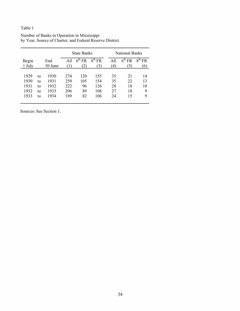
34

Table 1

Number of Banks in Operation in Mississippi by Year, Source of Charter, and Federal Reserve District

State Banks National Banks

Begin End All 6th FR 8th FR All 6th FR 8th FR 1 July 30 June (1) (2) (3) (4) (5) (6)

1929 to 1930 274 120 155 35 21 14 1930 to 1931 259 105 154 35 22 13 1931 to 1932 222 96 126 28 18 10 1932 to 1933 206 89 108 27 18 91933 to 1934 189 82 106 24 15 9

Sources: See Section 1.

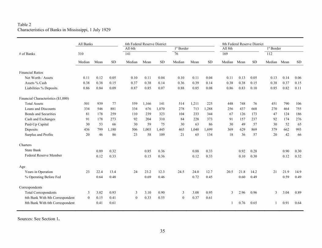
35

Table 2 Characteristics of Banks in Mississippi, 1 July 1929

All Banks 6th Federal Reserve District 8th Federal Reserve District All 6th 1º Border All 8th 1º Border # of Banks 310 141 76 169 112

Median Mean SD Median Mean SD Median Mean SD Median Mean SD Median Mean SD Financial Ratios Net Worth / Assets 0.11 0.12 0.05 0.10 0.11 0.04 0.10 0.11 0.04 0.11 0.13 0.05 0.13 0.14 0.06 Assets % Cash 0.38 0.38 0.15 0.37 0.38 0.14 0.36 0.39 0.14 0.38 0.38 0.15 0.38 0.37 0.15 Liabilities % Deposits 0.86 0.84 0.09 0.87 0.85 0.07 0.88 0.85 0.08 0.86 0.83 0.10 0.85 0.82 0.11 Financial Characteristics ($1,000) Total Assets 501 939 77 559 1,166 141 514 1,211 225 448 748 76 451 790 106 Loans and Discounts 334 546 881 334 676 1,070 278 713 1,288 256 437 668 270 464 755 Bonds and Securities 81 178 259 110 239 323 104 233 344 67 126 173 47 124 186 Cash and Exchanges 91 178 273 92 204 310 84 228 373 91 157 237 92 174 276 Paid-Up Capital 30 53 66 30 59 75 30 63 86 30 49 57 30 52 65 Deposits 436 799 1,180 506 1,003 1,445 465 1,040 1,699 369 629 869 379 662 993 Surplus and Profits 20 46 86 23 58 109 21 65 134 18 36 57 20 42 66 Charters

State Bank 0.89 0.32 0.85 0.36 0.88 0.33 0.92 0.28 0.90 0.30 Federal Reserve Member 0.12 0.33 0.15 0.36 0.12 0.33 0.10 0.30 0.12 0.32 Age Years in Operation 23 22.4 13.4 24 23.2 12.3 24.5 24.0 12.7 20.5 21.8 14.2 21 21.9 14.9 % Operating Before Fed 0.64 0.48 0.69 0.46 0.72 0.45 0.60 0.49 0.59 0.49 Correspondents Total Correspondents 3 3.02 0.93 3 3.10 0.90 3 3.08 0.95 3 2.96 0.96 3 3.04 0.89 6th Bank With 8th Correspondent 0 0.15 0.41 0 0.33 0.55 0 0.37 0.61 8th Bank With 6th Correspondent 0.41 0.61 1 0.76 0.65 1 0.91 0.64

Sources: See Section 1.

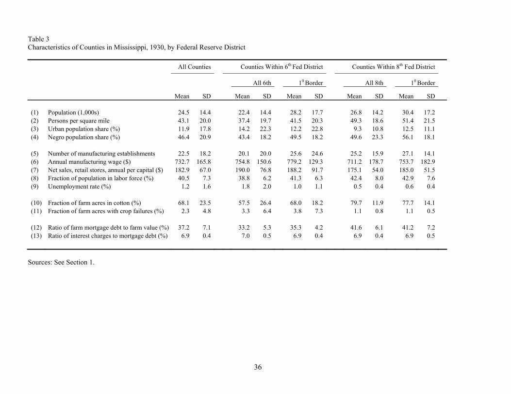
36

Table 3 Characteristics of Counties in Mississippi, 1930, by Federal Reserve District

All Counties Counties Within 6th Fed District Counties Within 8th Fed District

All 6th 10 Border All 8th 10 Border

Mean SD Mean SD Mean SD Mean SD Mean SD

(1) Population (1,000s) 24.5 14.4 22.4 14.4 28.2 17.7 26.8 14.2 30.4 17.2 (2) Persons per square mile 43.1 20.0 37.4 19.7 41.5 20.3 49.3 18.6 51.4 21.5 (3) Urban population share (%) 11.9 17.8 14.2 22.3 12.2 22.8 9.3 10.8 12.5 11.1 (4) Negro population share (%) 46.4 20.9 43.4 18.2 49.5 18.2 49.6 23.3 56.1 18.1 (5) Number of manufacturing establishments 22.5 18.2 20.1 20.0 25.6 24.6 25.2 15.9 27.1 14.1 (6) Annual manufacturing wage ($) 732.7 165.8 754.8 150.6 779.2 129.3 711.2 178.7 753.7 182.9 (7) Net sales, retail stores, annual per capital ($) 182.9 67.0 190.0 76.8 188.2 91.7 175.1 54.0 185.0 51.5 (8) Fraction of population in labor force (%) 40.5 7.3 38.8 6.2 41.3 6.3 42.4 8.0 42.9 7.6 (9) Unemployment rate (%) 1.2 1.6 1.8 2.0 1.0 1.1 0.5 0.4 0.6 0.4 (10) Fraction of farm acres in cotton (%) 68.1 23.5 57.5 26.4 68.0 18.2 79.7 11.9 77.7 14.1 (11) Fraction of farm acres with crop failures (%) 2.3 4.8 3.3 6.4 3.8 7.3 1.1 0.8 1.1 0.5 (12) Ratio of farm mortgage debt to farm value (%) 37.2 7.1 33.2 5.3 35.3 4.2 41.6 6.1 41.2 7.2 (13) Ratio of interest charges to mortgage debt (%) 6.9 0.4 7.0 0.5 6.9 0.4 6.9 0.4 6.9 0.5

Sources: See Section 1.

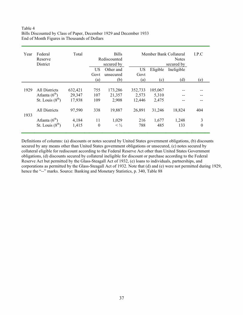
37

Table 4 Bills Discounted by Class of Paper, December 1929 and December 1933 End of Month Figures in Thousands of Dollars Year Federal

Reserve District

Total Bills Rediscounted

secured by

Member Bank Collateral Notes

secured by

US Govt

Other and unsecured

US Govt

Eligible Ineligible

I.P.C

(a) (b) (a) (c) (d) (e)

1929 All Districts 632,421 755 173,286 352,733 105,067 -- -- Atlanta (6th) 29,347 107 21,357 2,573 5,310 -- -- St. Louis (8th) 17,938 109 2,908 12,446 2,475 -- --

1933

All Districts 97,590 338 19,887 26,891 31,246 18,824 404

Atlanta (6th) 4,184 11 1,029 216 1,677 1,248 3 St. Louis (8th) 1,415 0 < ½ 788 485 133 0

Definitions of columns: (a) discounts or notes secured by United States government obligations, (b) discounts secured by any means other than United States government obligations or unsecured, (c) notes secured by collateral eligible for rediscount according to the Federal Reserve Act other than United States Government obligations, (d) discounts secured by collateral ineligible for discount or purchase according to the Federal Reserve Act but permitted by the Glass-Steagall Act of 1932, (e) loans to individuals, partnerships, and corporations as permitted by the Glass-Steagall Act of 1932. Note that (d) and (e) were not permitted during 1929, hence the “--” marks. Source: Banking and Monetary Statistics, p. 340, Table 88

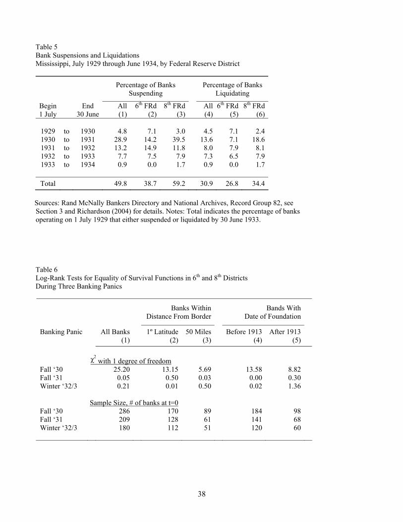
38

Table 5 Bank Suspensions and Liquidations Mississippi, July 1929 through June 1934, by Federal Reserve District Percentage of Banks

Suspending Percentage of Banks

Liquidating

Begin End All 6th FRd 8th FRd All 6th FRd 8th FRd1 July 30 June (1) (2) (3) (4) (5) (6)

1929 to 1930 4.8 7.1 3.0 4.5 7.1 2.41930 to 1931 28.9 14.2 39.5 13.6 7.1 18.61931 to 1932 13.2 14.9 11.8 8.0 7.9 8.11932 to 1933 7.7 7.5 7.9 7.3 6.5 7.91933 to 1934 0.9 0.0 1.7 0.9 0.0 1.7

Total 49.8 38.7 59.2 30.9 26.8 34.4

Sources: Rand McNally Bankers Directory and National Archives, Record Group 82, see Section 3 and Richardson (2004) for details. Notes: Total indicates the percentage of banks operating on 1 July 1929 that either suspended or liquidated by 30 June 1933. Table 6 Log-Rank Tests for Equality of Survival Functions in 6th and 8th Districts During Three Banking Panics

Banks Within Distance From Border

Bands With Date of Foundation

Banking Panic All Banks 1º Latitude 50 Miles Before 1913 After 1913 (1) (2) (3) (4) (5)

χ2 with 1 degree of freedom

Fall ‘30 25.20 13.15 5.69 13.58 8.82 Fall ‘31 0.05 0.50 0.03 0.00 0.30 Winter ‘32/3 0.21 0.01 0.50 0.02 1.36

Sample Size, # of banks at t=0 Fall ‘30 286 170 89 184 98 Fall ‘31 209 128 61 141 68 Winter ‘32/3 180 112 51 120 60

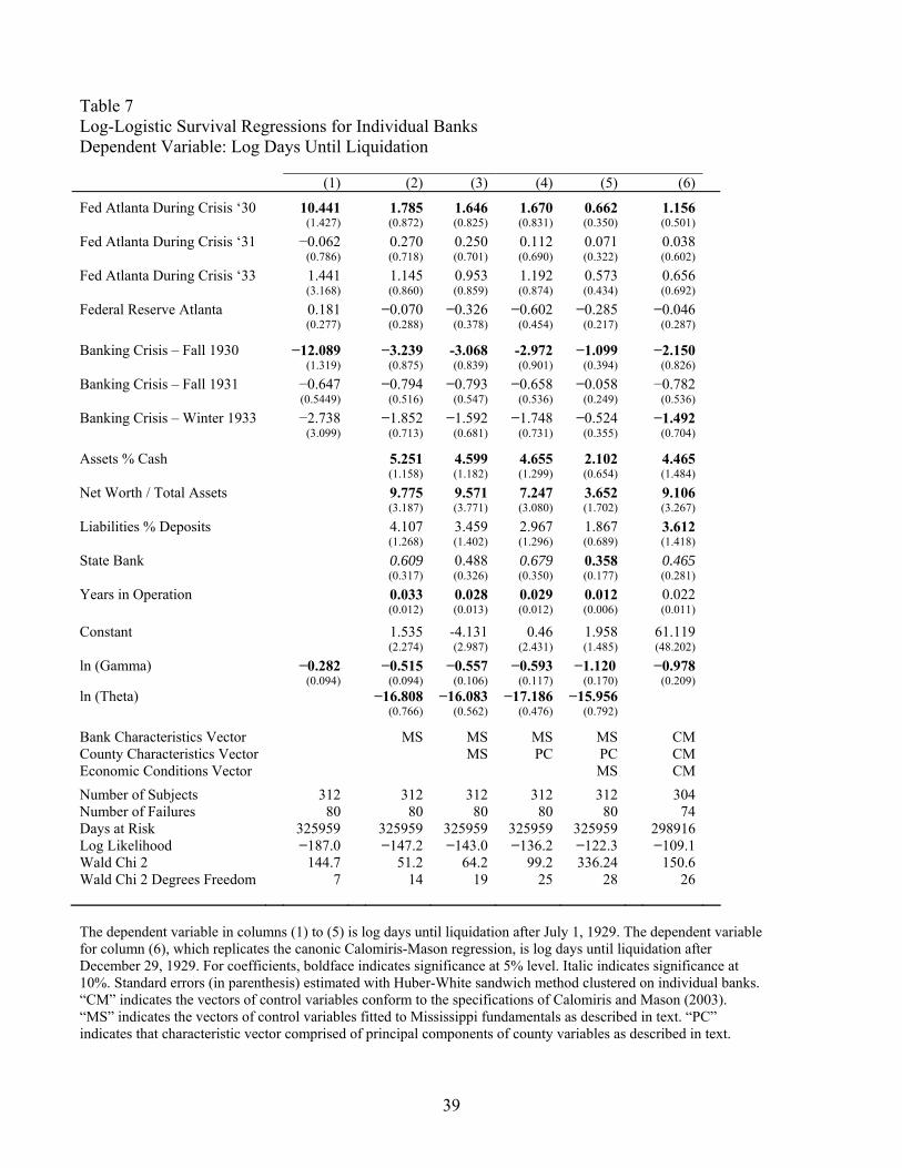
39

Table 7 Log-Logistic Survival Regressions for Individual Banks Dependent Variable: Log Days Until Liquidation (1) (2) (3) (4) (5) (6)

Fed Atlanta During Crisis ‘30 10.441 1.785 1.646 1.670 0.662 1.156 (1.427) (0.872) (0.825) (0.831) (0.350) (0.501)

Fed Atlanta During Crisis ‘31 −0.062 0.270 0.250 0.112 0.071 0.038 (0.786) (0.718) (0.701) (0.690) (0.322) (0.602)

Fed Atlanta During Crisis ‘33 1.441 1.145 0.953 1.192 0.573 0.656 (3.168) (0.860) (0.859) (0.874) (0.434) (0.692)

Federal Reserve Atlanta 0.181 −0.070 −0.326 −0.602 −0.285 −0.046 (0.277) (0.288) (0.378) (0.454) (0.217) (0.287)

Banking Crisis – Fall 1930 −12.089 −3.239 -3.068 -2.972 −1.099 −2.150 (1.319) (0.875) (0.839) (0.901) (0.394) (0.826)

Banking Crisis – Fall 1931 −0.647 −0.794 −0.793 −0.658 −0.058 −0.782 (0.5449) (0.516) (0.547) (0.536) (0.249) (0.536)

Banking Crisis – Winter 1933 −2.738 −1.852 −1.592 −1.748 −0.524 −1.492 (3.099) (0.713) (0.681) (0.731) (0.355) (0.704)

Assets % Cash 5.251 4.599 4.655 2.102 4.465 (1.158) (1.182) (1.299) (0.654) (1.484)

Net Worth / Total Assets 9.775 9.571 7.247 3.652 9.106 (3.187) (3.771) (3.080) (1.702) (3.267)

Liabilities % Deposits 4.107 3.459 2.967 1.867 3.612 (1.268) (1.402) (1.296) (0.689) (1.418)

State Bank 0.609 0.488 0.679 0.358 0.465 (0.317) (0.326) (0.350) (0.177) (0.281)

Years in Operation 0.033 0.028 0.029 0.012 0.022 (0.012) (0.013) (0.012) (0.006) (0.011)

Constant 1.535 -4.131 0.46 1.958 61.119 (2.274) (2.987) (2.431) (1.485) (48.202)

ln (Gamma) −0.282 −0.515 −0.557 −0.593 −1.120 −0.978 (0.094) (0.094) (0.106) (0.117) (0.170) (0.209) ln (Theta) −16.808 −16.083 −17.186 −15.956

(0.766) (0.562) (0.476) (0.792)

Bank Characteristics Vector MS MS MS MS CM County Characteristics Vector MS PC PC CM Economic Conditions Vector MS CM

Number of Subjects 312 312 312 312 312 304 Number of Failures 80 80 80 80 80 74 Days at Risk 325959 325959 325959 325959 325959 298916 Log Likelihood −187.0 −147.2 −143.0 −136.2 −122.3 −109.1 Wald Chi 2 144.7 51.2 64.2 99.2 336.24 150.6 Wald Chi 2 Degrees Freedom 7 14 19 25 28 26 The dependent variable in columns (1) to (5) is log days until liquidation after July 1, 1929. The dependent variable for column (6), which replicates the canonic Calomiris-Mason regression, is log days until liquidation after December 29, 1929. For coefficients, boldface indicates significance at 5% level. Italic indicates significance at 10%. Standard errors (in parenthesis) estimated with Huber-White sandwich method clustered on individual banks. “CM” indicates the vectors of control variables conform to the specifications of Calomiris and Mason (2003). “MS” indicates the vectors of control variables fitted to Mississippi fundamentals as described in text. “PC” indicates that characteristic vector comprised of principal components of county variables as described in text.

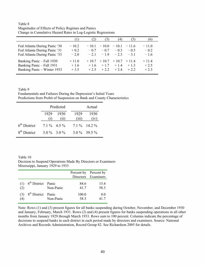
40

Table 8 Magnitudes of Effects of Policy Regimes and Panics Change in Cumulative Hazard Rates in Log-Logistic Regressions

(1) (2) (3) (4) (5) (6)

Fed Atlanta During Panic ‘30 − 10.2 − 10.1 − 10.0 − 10.1 − 11.6 − 11.0 Fed Atlanta During Panic ‘31 + 0.2 − 0.7 − 0.7 − 0.3 − 0.5 − 0.2 Fed Atlanta During Panic ‘33 − 2.0 − 2.1 − 1.9 − 2.3 − 3.1 − 1.6

Banking Panic – Fall 1930 + 11.0 + 10.7 + 10.7 + 10.7 + 11.4 + 11.4 Banking Panic – Fall 1931 + 1.6 + 1.6 + 1.7 + 1.4 + 1.3 + 2.5 Banking Panic – Winter 1933 + 3.5 + 2.5 + 2.2 + 2.4 + 2.2 + 2.3

Table 9 Fundamentals and Failures During the Depression’s Initial Years Predictions from Probit of Suspension on Bank and County Characteristics

Predicted Actual

1929 1930 1929 1930 (i) (ii) (iii) (iv)

6th District 7.1 % 4.5 % 7.1 % 14.2 %

8th District 3.0 % 3.0 % 3.0 % 39.5 %

Table 10 Decision to Suspend Operations Made By Directors or Examiners Mississippi, January 1929 to 1933

Percent by Directors

Percent by Examiners

(1) 6th District Panic 84.6 15.4(2) Non-Panic 41.7 58.3

(3) 8th District Panic 100.0 0.0(4) Non-Panic 58.3 41.7

Note: Rows (1) and (3) present figures for all banks suspending during October, November, and December 1930 and January, February, March 1931. Rows (2) and (4) present figures for banks suspending operations in all other months from January 1929 through March 1933. Rows sum to 100 percent. Columns indicate the percentage of decisions to suspend banks in each district in each period made by directors and examiners. Source: National Archives and Records Administration, Record Group 82. See Richardson 2005 for details.

41

Table 11 Causes of Bank Suspensions Mississippi, January 1929 through March 1933

Correspondents

(i)

Runs Only

(ii)

Runs Primary

(iii)

Assets Primary

(iv)

Assets Only

(v)

(1) 6th District Panic 0.0 23.1 15.4 61.5 0.0 (2) Non-Panic 0.0 8.3 29.2 50.0 12.5 (3) 8th District Panic 19.0 34.5 3.4 41.4 1.7 (4) Non-Panic 4.2 20.8 29.2 25.0 20.8

Note: Rows defined as in Table 9. Columns indicate the percentage of suspended banks in each district in each period whose cause of suspension was judged to be due to the closure of correspondents, due to runs only, due primarily to runs but with contributing causes (usually frozen assets), due primarily to asset problems but with contributing causes (usually heavy withdrawals), or due to asset problems only. Source: Richardson 2004. Table 12 Asset Quality at Suspended Banks Mississippi, January 1929 through March 1933

Percent Good

Percent Problematic

(1) 6th District Panic 23.1 76.9(2) Non-Panic 8.3 91.7 (3) 8th District Panic 53.4 46.6(4) Non-Panic 25.0 75.0

Note: Rows defined as in Table 9. Columns indicate the percentage of suspended banks in each district in each period whose assets were judged by examiners to be good, and thus, neither to have been a primary nor a contributing cause of the suspension, and problematic (i.e. either slow, doubtful, or worthless) and to have been either a primary or contributing cause of the suspension. Source: Richardson 2004. Table 13 Percentage of Assets Recovered By End of 1931 for Banks Which Ceased Operations From October 1930 through January 1931

FR District 6th 8th

Percent Recovered 0.475 0.295 Standard Deviation 0.159 0.165 Sample Size 6 33

Source: Mississippi State Banking Department, 1931 and 1933.

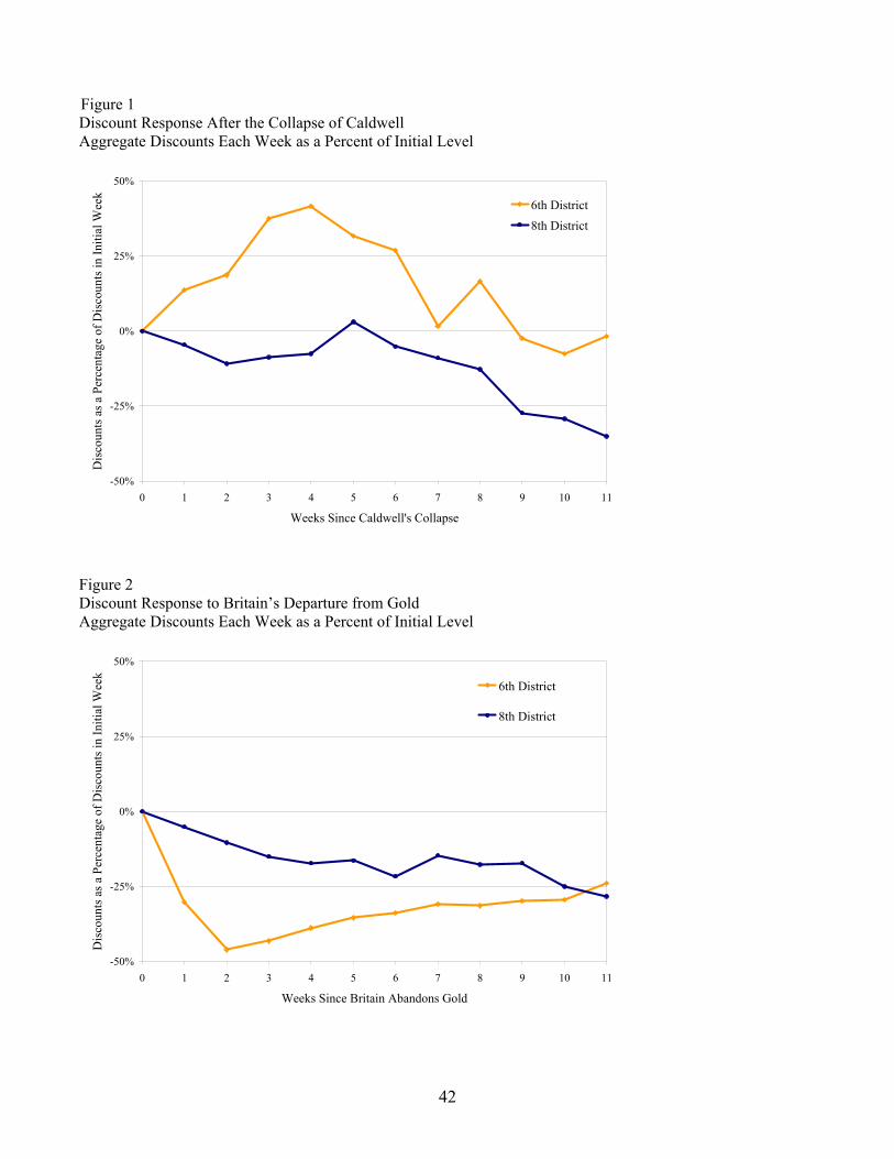
42

Figure 1 Discount Response After the Collapse of Caldwell Aggregate Discounts Each Week as a Percent of Initial Level

-50%

-25%

0%

25%

50%

0 1 2 3 4 5 6 7 8 9 10 11

Weeks Since Caldwell's Collapse

Dis

coun

ts a

s a P

erce

ntag

e of

Dis

coun

ts in

Initi

al W

eek

6th District8th District

Figure 2 Discount Response to Britain’s Departure from Gold Aggregate Discounts Each Week as a Percent of Initial Level

-50%

-25%

0%

25%

50%

0 1 2 3 4 5 6 7 8 9 10 11

Weeks Since Britain Abandons Gold

Dis

coun

ts a

s a P

erce

ntag

e of

Dis

coun

ts in

Initi

al W

eek

6th District

8th District

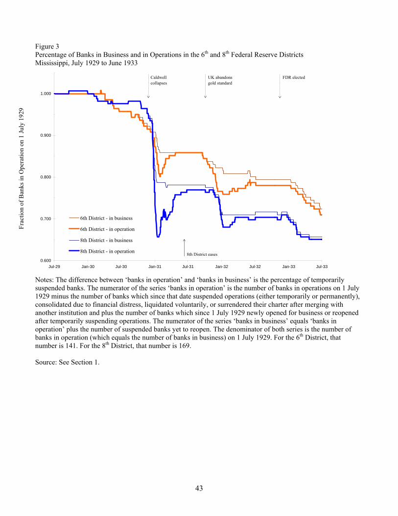
43

Figure 3 Percentage of Banks in Business and in Operations in the 6th and 8th Federal Reserve Districts Mississippi, July 1929 to June 1933

0.600

0.700

0.800

0.900

1.000

Jul-29 Jan-30 Jul-30 Jan-31 Jul-31 Jan-32 Jul-32 Jan-33 Jul-33

6th District - in business

6th District - in operation

8th District - in business

8th District - in operation

Caldwell collapses

UK abandons gold standard

FDR elected

8th District eases Glass-Steagall Feb. '32

Notes: The difference between ‘banks in operation’ and ‘banks in business’ is the percentage of temporarily suspended banks. The numerator of the series ‘banks in operation’ is the number of banks in operations on 1 July 1929 minus the number of banks which since that date suspended operations (either temporarily or permanently), consolidated due to financial distress, liquidated voluntarily, or surrendered their charter after merging with another institution and plus the number of banks which since 1 July 1929 newly opened for business or reopened after temporarily suspending operations. The numerator of the series ‘banks in business’ equals ‘banks in operation’ plus the number of suspended banks yet to reopen. The denominator of both series is the number of banks in operation (which equals the number of banks in business) on 1 July 1929. For the 6th District, that number is 141. For the 8th District, that number is 169. Source: See Section 1.

Frac

tion

of B

anks

in O

pera

tion

on 1

July

192

9

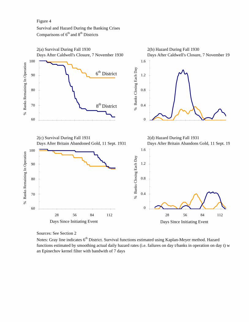
Figure 4Survival and Hazard During the Banking CrisesComparisons of 6th and 8th Districts

2(a) Survival During Fall 1930 2(b) Hazard During Fall 1930Days After Caldwell's Closure, 7 November 1930 Days After Caldwell's Closure, 7 November 19

2(c) Survival During Fall 1931 2(d) Hazard During Fall 1931Days After Britain Abandoned Gold, 11 Sept. 1931 Days After Britain Abandons Gold, 11 Sept. 19

Sources: See Section 2Notes: Gray line indicates 6th District. Survival functions estimated using Kaplan-Meyer method. Hazardfunctions estimated by smoothing actual daily hazard rates (i.e. failures on day t/banks in operation on day t) wan Epinechov kernel filter with bandwith of 7 days

28

Days Since Initiating Event56 84 112 28

Days Since Initiating Event56 84 112

% B

anks

Rem

aini

ng In

Ope

ratio

n 100

90

80

70

60

% B

anks

Rem

aini

ng In

Ope

ratio

n 100

90

80

70

60

% B

anks

Clo

sing

Eac

h D

ay

1.6

1.2

0.8

0.4

0

% B

anks

Clo

sing

Eac

h D

ay

1.6

1.2

0.8

0.4

0

6th District

8th District

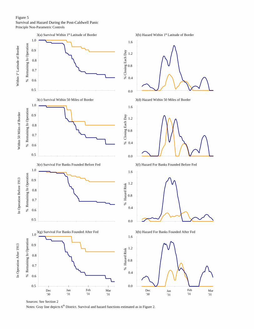
Figure 5Survival and Hazard During the Post-Caldwell PanicPrinciple Non-Parametric Controls

3(c) Survival Within 50 Miles of Border 3(d) Hazard Within 50 Miles of Border

3(e) Survival For Banks Founded Before Fed 3(f) Hazard For Banks Founded Before Fed

3(g) Survival For Banks Founded After Fed 3(h) Hazard For Banks Founded After Fed

Sources: See Section 2Notes: Gray line depicts 6th District. Survival and hazard functions estimated as in Figure 2.

3(b) Hazard Within 1º Latitude of Border

In O

pera

tion

Afte

r 191

3

3(a) Survival Within 1º Latitude of Border

With

in 1

º Lat

itude

of B

orde

rW

ithin

50

Mile

s of B

orde

rIn

Ope

ratio

n B

efor

e 19

13

Dec'30

Dec'30

Jan'31

Feb'31

Mar'31

Jan'31

Feb'31

Mar'31

1.6

1.2

0.8

0.4% C

losi

ng E

ach

Day

0.0

1.6

1.2

0.8

0.4% C

losi

ng E

ach

Day

0.0

1.6

1.2

0.8

0.4

% H

azar

d R

isk

0.0

1.6

1.2

0.8

0.4

% H

azar

d R

isk

0.0

1.0

0.9

0.8

0.7

% R

emai

ning

In O

pera

tion

0.6

0.5

1.0

0.9

0.8

0.7

% R

emai

ning

In O

pera

tion

0.6

0.5

1.0

0.9

0.8

0.7

% R

emai

ning

In O

pera

tion

0.6

0.5

1.0

0.9

0.8

0.7

% R

emai

ning

In O

pera

tion

0.6

0.5

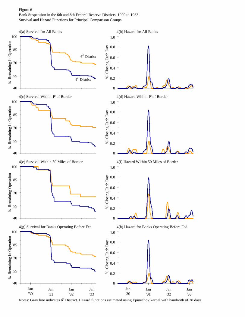
Figure 6Bank Suspension in the 6th and 8th Federal Reserve Districts, 1929 to 1933Survival and Hazard Functions for Principal Comparison Groups

4(a) Survival for All Banks 4(b) Hazard for All Banks

4(c) Survival Within 1º of Border 4(d) Hazard Within 1º of Border

4(e) Survival Within 50 Miles of Border 4(f) Hazard Within 50 Miles of Border

4(g) Survival for Banks Operating Before Fed 4(h) Hazard for Banks Operating Before Fed

Notes: Gray line indicates 6th District. Hazard functions estimated using Epinechov kernel with bandwith of 28 days.

Jan'30

Jan'31

Jan'32

Jan'33

1.0

0.8

0.6

0.4

% C

losi

ng E

ach

Day

0.2

0

100

85

70

55

% R

emai

ning

In O

pera

tion

40

Jan'30

Jan'31

Jan'32

Jan'33

6th District

8th District

1.0

0.8

0.6

0.4

% C

losi

ng E

ach

Day

0.2

0

1.0

0.8

0.6

0.4

% C

losi

ng E

ach

Day

0.2

0

1.0

0.8

0.6

0.4

% C

losi

ng E

ach

Day

0.2

0

100

85

70

55

% R

emai

ning

In O

pera

tion

40

100

85

70

55

% R

emai

ning

Ope

ratio

n

40

100

85

70

55

% R

emai

ning

In O

pera

tion

40

47

Bibliography

Anderson, Clay J. A Half-Century of Federal Reserve Policymaking, 1914-1964. Philadelphia: Federal Reserve Bank of Philadelphia, 1965.

Bagehot, Walter. Lombard Street: A Description of the Money Market. New York: Scriber, Armstrong and

Company, 1873. Bernanke, B. S. “Nonmonetary Effects of the Financial Crisis in the Propagation of the Great Depression.”

American Economic Review, June 1983, (73), pp. 257-276. Board of Governors of the Federal Reserve System. Annual Report. Washington, D.C.: Government Printing

Office. Various dates 1928 to 1933. ----- Banking and Monetary Statistics, 1914-1941. Washington, D.C.: Federal Reserve System, 1943. Bradstreet’s Weekly. New York: Bradstreet Company, various issues. Calomiris, Charles W. and Joseph R. Mason. “Contagion and Bank Failures During The Great Depression: The

June 1932 Chicago Banking Panic.” American Economic Review, December 1997, 87(5), pp. 863-883. ----- “Fundamentals, Panics, and Bank Distress During the Depression.” American Economic Review, December

2003, 93(5): pp. 1615-1646. Carlson, Mark. “Are Branch Banks Better Survivors? Evidence from the Depression Era.” Economic Inquiry,

January 2004, (42), pp. 111-126 Cecchetti, Stephen G and Karras, Georgios. “Sources of Output Fluctuations during the Interwar Period: Further

Evidence on the Causes of the Great Depression.” The Review of Economics and Statistics, 1994, 76(1): pp. 80-102

Chandler, Lester Vernon. American Monetary Policy 1928-1941. Harper and Row Publishers, 1971. Christiano, Lawrence J., Roberto Motto, and Massimo Rostagno. “The Great Depression and the Friedman-

Schwartz Hypothesis,” Working Paper 0318, Federal Reserve Bank of Cleveland. 2004. Clark, Lawrence E. Central Banking Under the Federal Reserve System. New York: Macmillan, 1935. Commercial and Financial Chronicle. New York: William B. Dana Company. Various issues. Diamond, Douglas W. and Philip H. Dybvig. “Bank Runs, Deposit Insurance, & Liquidity,” Journal of Political

Economy, 1983, Vol. 91, pp. 401-419. Dun’s Review: A Weekly Survey of Business Conditions in the United States and Canada. R.G. Dun and

Company, various issues 1928 to 1935. Eichengreen, Barry. Golden Fetters. New York: Oxford University Press, 1992. Friedman, Milton and Anna J. Schwartz. A Monetary History of the United States, 1867-1960. Princeton:

Princeton University Press for the National Bureau of Economic Research. 1963. Gamble, Richard. A History of the Federal Reserve Bank of Atlanta, 1914-1989. Federal Reserve Bank of Atlanta,

48

1989. Goldenweiser, Emanuel A. American Monetary Policy. New York: McGraw-Hill for the Committee on Economic

Development. 1951. Hardy, Charles O. Credit Policies of the Federal Reserve System. Washington, D.C.: The Brookings Institution,

1932. Historical, Demographic, Economic, and Social Data: The United States, 1790-1970. Intrauniversity Consortium

for Political and Social Research Study # 3. Ann Arbor, MI: University of Michigan and ICPSR. Jacklin, C. and Bhattacharya, S. 1988. “Distinguishing Panics and Information-Based Bank Runs: Welfare Policy

Implications.” Journal of Political Economy, June 1988, (96), pp. 568-592. Martin, Antoine. “Liquidity Provision vs. Deposition Insurance: Preventing Bank Panics Without Moral Hazard.”

RWP 01-05. Federal Reserve Bank of Kansas City, September 2004. McFerrin, J. B. 1969. Caldwell and Company. North Carolina University Press. 1939. Meltzer, Allan H. “Monetary and Other Explanations for the Start of the Great Depression.” Journal of Monetary

Economics 2 (1976): 455-72. ----- A History of the Federal Reserve, Volume 1, 1913-1951. Chicago: University of Chicago Press, 2003. Mississippi Banking Department. Biennial Report of the Banking Department of the State of Mississippi. Various

issues 1916 to 1939. Mitchener, Kris. “Are Prudential Supervision and Regulation Pillars of Financial Stability? Evidence from the

Great Depression.” Leavey Business School Working Paper 03/04-06-WP. 2004. Moore, Carl H. The Federal Reserve System: a history of the first 75 years. McFarland and Company, Inc, 1990. Rand-McNally Bankers’ Directory. Rand McNally: Chicago. Various issues 1929 through July 1935. Richardson, Gary. “Categories and Causes of Bank Distress, 1929 to 1933, New Data from the Archives of the

Board of Governors.” UC Irvine Mimeo, 2004. ----- “The Central Subject File of the Federal Reserve Board of Governors, 1913 to 1954: An Archival Survey.”

Journal of Financial History (expected spring 2006). Richardson, Gary and William Troost. “Monetary Intervention Mitigated Banking Panics During the Great

Depression: Additional Evidence and Robustness Checks.” UC Irvine Mimeo, 2005. Romer, Christina. “The Nation in Depression.” The Journal of Economic Perspectives. Vol 7, No. 2 (Spring,

1993), pp. 19-39.

Romer, Christina and David Romer. “Does Monetary Policy Matter? A New Test in the Spirit of Friedman and Schwartz.” In Olivier Blanchard and Stanley Fischer, eds., NBER Macroeconomics Annual, Cambridge MA: MIT Press. 1989.

Rosenbloom, Joshua and William Sundstrom. “The Sources of Regional Variation in the Severity of the Great Depression: Evidence from U.S. Manufacturing, 1919-1937.” Journal of Economic History 59, September

49

1999, pp. 714-747. Thomas, Lloyd B. Money, Banking, and Financial Markets. New York: Thomson, South-Western. 2005 Temin, Peter. Did Monetary Forces Cause the Great Depression? New York: W.W. Norton, 1976. ---- Lessons from the Great Depression. Cambridge, MA: MIT Press, 1989. Warburton, Clark. Deposit Guaranty in Mississippi. Manuscript, Division of Research and Statistics, Federal

Reserve Deposit Corporation, 1955. Westerfield, Ray B. Marginal Collateral to Discounts at the Federal Reserve Banks. American Economic Review,

Vol. 22, No. 1, March 1932, pp. 34-55. Wheelock, David. “Member Bank Borrowing and the Fed’s Contractionary Monetary Policy During the Great

Depression.” Journal of Money, Credit and Banking November 1990, (22) pp. 409-426. ----- The Strategy and Consistency of Federal Reserve Monetary Policy, 1924-1933. Cambridge University Press,

1991. Whitney, Caroline. Experiments in Credit Control, The Federal Reserve System. New York: Columbia University

Press, 1934. Wicker, Elmus. Federal Reserve Monetary Policy: 1917-1933. New York: Random House, 1966. ----- The Banking Panics of the Great Depression. Cambridge: Cambridge University Press, 1996.