arX

iv:1

006.

1351

v2 [

astr

o-ph

.CO

] 1

5 D

ec 2

010

Mon. Not. R. Astron. Soc. 000, 000–000 (0000) Printed 3 November 2021 (MN LATEX style file v2.2)

The GMRT Epoch of Reionization Experiment: A new

upper limit on the neutral hydrogen power spectrum at

z ≈ 8.6

Gregory Paciga1⋆, Tzu-Ching Chang1,2, Yashwant Gupta3, Rajaram Nityanada3,

Julia Odegova1, Ue-Li Pen1†, Jeffrey B. Peterson4, Jayanta Roy3, Kris Sigurdson51 CITA, University of Toronto, 60 St George Street, Toronto, ON M5S 3H8, Canada2 IAA, Academia Sinica, P.O. Box 23-141, Taipei 10617, Taiwan3 National Center for Radio Astrophysics, Tata Institute for Fundamental Research, Pune 411 007, India4 Department of Physics, Carnegie Mellon University, 5000 Forbes Ave, Pittsburgh, PA 15213, USA5 Department of Physics and Astronomy, University of British Columbia, Vancouver, BC V6T 1Z1, Canada

3 November 2021

ABSTRACT

We present a new upper limit to the 21 cm power spectrum during the Epoch ofReionization (EoR) which constrains reionization models with an unheated IGM. TheGMRT-EoR experiment is an ongoing effort to make a statistical detection of the powerspectrum of 21 cm neutral hydrogen emission at redshift z ∼ 9. Data from this redshiftconstrain models of the EoR, the end of the Dark Ages arising from the formation ofthe first bright UV sources, probably stars or mini-quasars. We present results fromapproximately 50 hours of observations at the Giant Metrewave Radio Telescope inIndia from December 2007. We describe radio frequency interference (RFI) localisationschemes which allow bright sources on the ground to be identified and physicallyremoved in addition to automated flagging. Singular-value decomposition is used toremove remaining broadband RFI by identifying ground sources with large eigenvalues.Foregrounds are modelled using a piecewise linear filter and the power spectrum ismeasured using cross-correlations of foreground subtracted images.

Key words: cosmology: observations – intergalactic medium – radio lines: general –diffuse radiation

1 INTRODUCTION

Between the recombination epoch at z ∼ 1100 and thefirst round of star formation at z ∼ 10 the Universe wasfilled with neutral hydrogen. This neutral gas is thought tohave produced 21 cm hyperfine emission with an effectivecontinuum brightness temperature between -500 and 30mK(Furlanetto et al. 2006) using z = 8.6 and WMAP 7-yearcosmological parameters (Komatsu et al. 2010), which haveformal error bars of roughly 10 per cent. As the first starsformed, beginning at local peaks in the matter density, thehydrogen gas was locally ionized. This is the start of a periodof cosmic evolution called the Epoch (or Era) of Reionization(EoR). Over time the ionized cells grew and overlapped, cre-ating a patchwork of ionized and neutral cells. This generalpatchy topology is well motivated by theory and simulations

⋆ Email:paciga@astro.utoronto.ca† Email:pen@cita.utoronto.ca

(e.g. Furlanetto et al. 2004; Iliev et al. 2006; McQuinn et al.2007; Zahn et al. 2007; see Trac & Gnedin 2009 for a review)though the exact properties are poorly constrained. Even-tually, by z ∼ 6, the ionization of the broadly distributedmaterial was complete, leaving only rare pockets of neutralgas.

In addition to directly constraining the redshift oflast scattering zls ∼ 1100, Cosmic Microwave Background(CMB) polarization data have been used to constrainthe redshift to the range 8.0 < z < 12.8 (WMAP7;Komatsu et al. 2010) under the assumption it was instan-taneous, although evidence from the CMB indicates thatreionization was an extended process (Dunkley et al. 2009).There is also substantial information on the neutral contentof the intergalactic medium (IGM) since z ∼ 6 via observa-tions of the Gunn-Peterson trough (Gunn & Peterson 1965)in quasar spectra (Djorgovski et al. 2001; Becker et al. 2001;Fan et al. 2006; Willott et al. 2007). Lyman-alpha (Ly-α)absorption provides a sensitive probe of neutral gas density

c© 0000 RAS

2 G. Paciga et al.

and can be used to constrain reionization (e.g., Fan et al.2002). With these two techniques we can observe the startand the end of the neutral era. However, neither CMB norquasar observations allow detailed examination of the reion-ization era itself. For this it has long been proposed to use21 cm fluctuations in the brightness temperature of neu-tral hydrogen (Sunyaev & Zeldovich 1975; Hogan & Rees1979). The 21 cm power spectrum, resulting from a com-bination of the patchy ionized and neutral medium andthe underlying mass power spectrum, is generally con-sidered one of the most promising signals (Scott & Rees1990; Zaldarriaga et al. 2004) and much attention has beenpaid in the literature toward designing suitable experimentsto detect it (e.g., Morales & Hewitt 2004; Morales 2005;Bowman et al. 2006; Harker et al. 2010).

Here the observing frequency is 1420MHz(1 + z)−1,in the very high frequency (VHF) range of the radiospectrum near 150MHz. Several programs are underwayto study the EoR in the VHF band including LOFAR1

(Kassim et al. 2004; Rottgering et al. 2006; for the EoRcase see, e.g., Zaroubi & Silk 2005; Harker et al. 2010),MWA2 (Lonsdale et al. 2009; for the EoR case see, e.g.,Morales et al. 2006; Bowman et al. 2006; Lidz et al. 2008),PAPER3 (Parsons et al. 2010), 21CMA4 (a.k.a. PaST;Peterson et al. 2004), in addition to the current GMRT5

program, and the first goal of such efforts is to determinethe redshift at which roughly half the volume of the uni-verse is ionized. Because the 21 cm emission is an isolatedsingle line, these observations can provide three dimensionalinformation over a large redshift range (Loeb & Zaldarriaga2004; Furlanetto et al. 2006), allowing a broad search forthe half-ionization redshift. In the future 21 cm tomographyhas the potential to add strong constraints on cosmologicalparameters (e.g., McQuinn et al. 2006; Cooray et al. 2008;Mao et al. 2008; Furlanetto et al. 2009; Masui et al. 2010).

The brightness temperature of the 21 cm line relativeto the CMB is determined by the ionization fraction ofhydrogen and the spin temperature of the neutral popu-lation, which is in turn governed by the background radia-tion and the kinetic temperature of the gas (Purcell & Field1956; Field 1959; Furlanetto et al. 2006). Reionization re-quires a minimum expenditure of 13.6 eV of energy per hy-drogen atom. In contrast, Ly-α photons, when absorbed bya neutral atom, are quickly re-emitted. Ly-α photons aresaid to undergo ‘resonant scattering’ and each (multiply-scattered) photon can affect many atoms before cosmic red-shifting makes them ineffective (Wouthuysen 1952; Field1959; Chuzhoy & Shapiro 2006). This means Ly-α pumpingof the hyperfine transition requires only about 1 per centof the UV flux required for ionization. Assuming a gradualincrease in UV flux with time, well before flux levels forreionization are reached, Ly-α pumping will couple the spintemperature to the kinetic temperature of the gas. If therewas no source of heat at that era other than a weak UV flux,the gas kinetic temperature must have been at its adiabatic

1 http://www.lofar.org/2 http://www.mwatelescope.org/3 http://astro.berkeley.edu/~dbacker/eor/4 http://web.phys.cmu.edu/~past/5 http://gmrt.ncra.tifr.res.in/

expansion value 1.7K at z = 8.5, and neutral gas will pro-duce a signal due to absorption of CMB photons in excess ofstimulated emission and ionized structures would be seen aslow-brightness regions on the sky (Chen & Miralda-Escude2004). In such a cold-gas model the brightness temperatureof the neutral gas against the CMB can be as low as -500mK.

A small fraction of the mass will have collapsed intominihaloes, which have a temperature higher than this adi-abatic temperature (Shapiro et al. 2006). This fraction mayeven be substantially smaller due to non-perturbative veloc-ity flows (Tseliakhovich & Hirata 2010; Dalal et al. 2010).No study was found on the impact of these non-linear effectson the Ly-α pumped IGM temperature. At linear order, thepositive and negative over and under densities cancel, andthe non-linear collapse fraction is still small, so we expectthe realistic value to be similar to the adiabatic prediction.

Alternatively, X-rays from supernovae or QSOsmight have heated the IGM above the CMB temper-ature of ≈ 30K before reionization (Madau et al. 1997;Chen & Miralda-Escude 2004). X-ray heating between 30Kand 10 000K will result in a largely neutral but warm IGM,which would be seen in emission. In the limit that Ts ≫ 30K,the volume emissivity becomes independent of tempera-ture. Patchy X-ray heating can also result in large angu-lar scale structure (Alvarez et al. 2010). The sky brightnesstemperature of the neutral gas has an asymptote at ∼ 30mK(Furlanetto et al. 2006).

The cosmic luminosity of X-rays at z ∼ 9 is notknown and difficult to estimate (see e.g., Dijkstra et al.2004; Salvaterra et al. 2007; Guo et al. 2009). If the rate ofcore collapse SNe at high redshift matches that of today,the X-ray output at z ∼ 9 would have been sufficient toraise the IGM temperature above the CMB temperature atthe onset of reionization. However, the mechanism of andfactors affecting core-collapse are not known and most nu-merical models appear to generically not result in SNe at all(Mezzacappa 2005). It is possible that at high z, core col-lapse SNe were not as abundant as today, and the IGM wasstill in absorption during the EoR. We therefore consider twolimits: one where the IGM is still cold and Tb = −500mK,and another where it is heated above CMB and Tb = 30mK.A general parametrization of these scenarios was recentlyproposed by Pritchard & Loeb (2010).

The GMRT-EoR project uses the Giant Metrewave Ra-dio Telescope (GMRT; Ananthakrishnan 1995) near Pune,India, to make measurements of the power spectrum of theneutral hydrogen signal with the hope of characterizing thestructure in the range 8.1 < z < 9.2. The FWHM of theGMRT primary beam at 150MHz is 3.3◦ which provides acylindrical comoving survey volume of (280 h−1Mpc)3, withabout equal dimensions in three directions. The primary sen-sitivity comes from the compact central core which is con-tained within ≈ 1 km, or 30 dish diametres, which gives im-ages with ∼ 302 resolution elements. As recorded, the datahave high spectral resolution along the line of sight, but webin the data for comparable transverse and radial resolution.Each data cube has ∼ 303 ≈ 30000 resolution elements soeven though the signal to noise ratio of each element is lessthan one, the spatial power can be measured to 1 per cent. Astatistical measurement of the power spectrum provides thebest hope of pinning down the EoR half-ionization redshift.

In section 2 we describe the data and analysis, including

c© 0000 RAS, MNRAS 000, 000–000

The GMRT-EoR Experiment: H I Power Spectrum 3

RFI removal and foreground filters used. In section 3 we ex-tend the analysis to cross-correlations of multiple nights, anda measurement of the power spectrum. We then conclude insection 4. All distances are in comoving coordinates.

2 OBSERVATIONS

2.1 GMRT and Data Description

The GMRT is a radio interferometer consisting of 30 an-tennas, each with a diametre of 45m. Fourteen of these arearranged in a dense central core within 1 km which allowsthe high brightness sensitivity required to search for thedim EoR signal (Pen et al. 2009). The longest separationbetween antennas is about 25 km. For this experiment thetelescope was operated at 150MHz with a 16.7MHz band-width. For 21 cm (1421MHz) emission, this frequency rangeprobes a redshift range of 8.1 < z < 9.2. The highest angu-lar resolution at this observing frequency at GMRT is about20 arcseconds.

Each antenna provides a pair of left and right circularlypolarized signals, which are passed through a new signalprocessing system, built in part for this project, called theGMRT Software Backend (GSB; Roy et al. 2010). The finalrecorded visibilities have a resolution of 7.8 kHz and 1/4 s infrequency and time, respectively.

The field is centred on the pulsar B0823+26. This pul-sar has a period of 0.53 seconds and an average flux of350mJy at 150MHz (Hobbs et al. 2004). It is situated ina relatively cold part of the sky at galactic latitude ≈ 30◦

with few nearby bright sources. The on-pulse flux is about6 Jy, brighter than all other sources in the field, making it agood calibrator. The calibration of this data was describedin Pen et al. (2009) and is summarized below. The positionsof the brightest sources in the field are shown in Fig. 1.

The data are folded in time into 16 ‘gates’ such thatthe pulse from the pulsar is contained within one gate. Theperiod of the pulsar is much shorter than the time-scale atwhich ionospheric fluctuations dominate, so by comparingthe ‘on’ gate with the neighbouring ‘off’ gates, everythingin the field that is constant over the period of the pulsar canbe removed. This includes sky sources and most radio fre-quency interference (RFI). By comparing the pulsar signalreceived by each antenna, the relative system gain of eachantenna can be calibrated. This technique allows calibrationof both phase and polarization in real time, with 100 percent observing efficiency, since no additional time is neededfor phase or flux calibration. Errors in clock synchronizationsometimes cause the pulsar pulse to straddle two gates. Inthese cases it is necessary to include the flanking gates whenidentifying the pulsar signal. This is not ideal since the pul-sar signal is diluted over multiple gates, but the correctionis limited to only the portion of observations that require it.

Since the pulsar amplitude varies from pulse to pulse,the absolute system gain needs to be measured separately.This is done using a noise injection system, which the GMRTsoftware backend decodes to calibrate the absolute gain ofthe system, while a sky radio source is used to transfer thenoise source calibration on to the sky. The primary fluxcalibrator used was 5C 7.245, a radio galaxy at z ≈ 1.6(Willott et al. 2001), located within the field of view (see

-3

-2

-1

0

1

2

3

-3 -2 -1 0 1 2 3

Rel

ativ

e D

eclin

atio

n [d

egre

es]

Relative Right Ascension [degrees]

N

E

3C 200

5C 7.245

B2 0825+24

B2 0819+25

PKS 0832+26

B2 0829+28

5C 7.111B2 0832+26A

B2 0828+27B2 0816+26B

5C 7.223B 0823+26

Figure 1. The 12 brightest sources in the field used for theseobservations. Pulsar PSR B0823+26 is at the centre of the field.The circle denotes the half-power diametre of the main beam.

Fig. 1). However, since this radio galaxy is an extended ob-ject, it can only be used as a calibrator for short baselineswhere its structure is not resolved. For antennas in longerbaselines we determine the relative gain calibration usingthe pulsar.

2.2 Data Analysis

Data from 2007 December 10, 11, 14, 16, 17, and 18 areincluded in the current analysis. A software pipeline hasbeen developed to automate the calibration and interfer-ence removal steps described below. The current configura-tion takes approximately 11 hours to process one hour ofdata on the CITA Sunnyvale computing cluster, or 20 hourson the National Centre for Radio Astronomy (NCRA) HPcomputing cluster in Pune, India. The NCRA facility canprocess four hours in parallel, completing one night of ob-servations in slightly less than two days. While the Sunny-vale cluster has the capacity to process as much as 12 hoursof data at once, storage capacity, shared usage, and otherbottlenecks reduce this significantly.

One of the limiting factors for measurement of theEoR signal is broadband radio frequency interference (RFI),which dominates the signal at 150MHz. In addition to thestandard procedure of flagging bad data, we also use a sin-gular value decomposition (SVD) to remove broadband RFIfrom the data, and also to identify and remove interferencesources. We believe this approach is unique among otherRFI mitigation strategies in the radio community.

Narrow line interference was removed by masking pointsin each frequency bin with an intensity above some thresh-old. This was done twice in the data reduction pipeline. In-put data are initially flagged with a threshold of 8σ on aGaussian scale, and then again at 3σ after broadband in-

c© 0000 RAS, MNRAS 000, 000–000

4 G. Paciga et al.

Figure 2. Representative stages in the data reduction pipeline.In each panel, the horizontal axis is frequency, covering approx-imately 1MHz, and the vertical is time, increasing downward,and covering approximately one hour. The grey-scale is the cross-power spectral density. The top row is the C0-C8 baseline and thebottom row the C0-W4 baseline, which are approximately 560mand 9400m respectively. Large bright patches indicate broadbandRFI, and vertical lines indicate line RFI. The first panel in eachrow is the initial input data. The second is after the initial 8σmask, with most interference still visible. The third panel is afterremoving the largest eigenvalues in the SVD. The broadband in-terference is no longer visible. The last panel shows the final 3σmask removing the line RFI, leaving a nearly uniform image.

terference was removed. The first mask can not be too ag-gressive or the techniques to remove broadband interference,discussed below, will fail.

Singular value decomposition (SVD) is used to separatebroadband radio sources on the ground from those in thesky. Ground-based sources contribute most to the largesteigenvalues since they do not move as a function of timewith respect to the array, while sky sources rotate. Onehour of data has 14396 time records, and each record hasabout 7.5 million entries corresponding to the number offrequency channels and baselines between the 60 antennas.This is treated as a matrix with each time record as onerow. The 50 largest eigenvalues are identified through anSVD and flagged as noise to be removed. A sample of thedata at a few intermediate stages showing the successful re-moval of both line and broadband RFI can be seen in Fig. 2.The RFI patterns in (u, v) space both before and after theSVD are illustrated in Fig. 3.

2.3 Physical Removal of Radio Interference

Sources

While some RFI can be removed in the data analysis, thisrisks removing sky signal as well. Ideally one would preventRFI from occurring at all by identifying and correcting thephysical sources. We can take advantage of the fact that asan interferometer GMRT is able to make images of the near-

Figure 3. Raw visibilities with (u, v) distance |b| < 200 be-fore the SVD RFI removal step (left) and after the RFI removal(right). The bright patterns in the central vertical strip (low |u|)are caused by RFI, and are significantly reduced by the SVD pro-cedure. The effect of this process on the final power spectrum isconsidered in section 3.2.

field, and create maps of bright RFI sources near the GMRTitself.

Candidate sources detected by a single baseline appearas a hyperbola of equal light arrival time in near-field imagesof a single SVD mode. When a source is detected by manybaselines, the corresponding hyperbolas intersect at a singlepoint in the image. These near-field images, an example ofwhich is shown in Fig. 4, become the ‘RFI maps’ whichare used to isolate interference sources. For sources with ahigh enough duty cycle, the GPS position given by the RFImaps are accurate enough that a handheld yagi antennaand portable radio receiver can be used to find the precisesource. With the handheld antenna direction to a sourcecan be determined by ear to better than 30 degrees, andthereafter localised by successive triangulation.

By comparing the position of a noise transmitter rela-tive to the candidate interference source both physically andin the RFI map, we can confirm whether we have identifiedthe correct source. Occasional misidentifications are likelydue to the intermittent nature of the sources; there is noguarantee that the radiating source in the images will stillbe active when an attempt at identification is made. Sincethe beginning of this effort, calibration has been improvedto locate sources within about 100m. Sources could in prin-ciple be located using only the array with a precision 10m,but the accuracy of available maps, GPS equipment, andother factors limit the real-world precision.

Candidate RFI sources identified so far include trans-formers, power line junctions, and loose wires in contact withpower lines. Table 1 lists some candidate sources recordedon 2008 December 6, and descriptions. In February 2009,GMRT began a collaboration effort with MSEDCL, whichcontrols the power transmission lines in the area aroundGMRT, to assist us in removing local interference sources.A wire hanging over 132 kV high tension power lines (#1 inTable 1) which was by far the brightest interference sourcewithin 20 km, appearing in 30 of the 50 largest eigenmodes,was removed in February 2009. Other bright sources havealso been removed since then. Although these sources arestill present in the raw data from 2007, this procedure hasshown that the SVD algorithm applied in the present workis successful in identifying real RFI sources during analysis.

c© 0000 RAS, MNRAS 000, 000–000

The GMRT-EoR Experiment: H I Power Spectrum 5

Table 1. List of candidate RFI sources based on observations on 2008 December 6, identified by the strongest SVD mode number fromwhich the GPS coordinates are derived. The two brightest sources, modes number 1 and 9, were removed in early 2009.

Mode Longitude Latitude Description

1 74.034653 19.147676 Conclusively identified as a wire hanging over 132 kV high tension power lines, clearly visibleusing the handheld yagi antenna several kilometres away. Wire removed with assistance fromMSEDCL on February 26, 2009.

9 74.085335 19.171797 Identified with wires hanging from an unused telephone pole, positioned directly under hightension lines.

13 74.034271 19.037518 Source in the area transmitted very intermittently, making identification difficult. Potentiallya transformer 20m north of coordinate.

14 74.096581 19.209597 Identified as a small wire hanging on a 500 kV power line, removed in February 2010.15 74.120018 19.181877 Two possible sources, both transmission towers, separated by about 300m. The one closest

to the coordinate is a T-junction of two high voltage lines.17 74.072952 19.088457 Initially identified to be a small pump approximately 150m west of this coordinate, though

other candidates include two nearby transformers.33 74.075623 19.108976 Transformer approximately 100m northwest, unambiguously radiating at low levels.

2.4 Single-night Images

After RFI removal has been completed in each one hourscan, polarization calibration is used to combine these intoimages of an entire night, typically of about 8 hours, as canbe seen in Fig. 5. This step accounts for leakage between theleft and right polarization signals, as well as effects causedby the relative rotation of the array and sky source by takinginto account the changing parallactic angle with time.

Although the array elements very nearly lie in a sin-gle plane, the rotation of the Earth turns this plane overtime with respect to the line of sight. To correctly stackmany hours together, one must consider the frequency anddirectional dependence of the measurement. One effect toconsider is the change of the primary beam with frequency.For a given frequency, the primary beam is well defined andindependent of (u, v). Deconvolution is difficult, but one canpick the frequency with the smallest beam and restrict thefield of view at other frequencies to match. Computation-ally this can be done by convolving with the ratio of thebeams, which is possible because of the commutativity ofthe primary beam operators.

However, this is a small effect compared to the effectsof a w term. Typically relative antenna positions are con-sidered to be on a two dimensional plane with coordinatesparametrized by (u, v) in units of the observing wavelength.Since baselines become non-coplanar over the course of thenight, a third dimension, w, must be included, without whichthe image becomes blurred.

For a thorough explanation of w term issues, see forexample Cornwell et al. (2008) and, for a more generaloverview, Thompson et al. (2001). As the observing fre-quency changes across the band, a single baseline samplesdifferent points in (u, v) space. At any given frequency, the(u, v) plane is typically sparsely sampled, but with manyfrequency channels there will often be data at a single (u, v)point for at least a few channels. One can subtract the aver-age from these, and under the assumption that foregroundsources have the same spectral index as the calibrator, thisremoves the foregrounds very well. Unfortunately, when con-sidering the full (u, v, w) cube, the data is too sparse for thisto work. Since the w coordinate is dependent on the positionin (u, v) space, and can become very large, the effects of the

w term can not be corrected at different frequencies in thesame way as the beam.

Strategies for correcting this effect for GMRT are be-ing developed, which build on those used in CMB studies(Myers et al. 2003; Hobson & Maisinger 2002), but we havenot yet applied these to our data. In the interim we restrictourselves to the short baselines for which w is small and suchcorrections are not needed. The short baselines are the onesmost sensitive to the EoR signal, so we retain most of theEoR sensitivity of the array.

The flux scale of the field is set by calibrating relativeto the pulsar in the centre of the field for every baseline,receiver, and frequency. Since the pulsar flux is known tobe variable, to set the absolute flux scale we identify thesource with the highest flux in the sky image, and set thispeak value equal to the known flux of that source. The ex-act value found depends on the angular resolution, deter-mined by the maximum baseline length used. For all daysanalysed in this work, the brightest apparent source is theradio galaxy 5C 7.245. The flux of this source was measuredas 215.1 ± 12.6mJy at 1415MHz by Willis et al. (1976) atthe Westerbork Radio Telescope, and as 685 ± 47mJy at408MHz in the 5C catalogue (Pearson & Kus 1978) for aspectral index of 0.93 ± 0.07. Following the same argumentas Pen et al. (2009), to achieve the best match with otherbright sources in the field, we adopt a value of 1.6 Jy for5C 7.245. Although the flux of this source changes by asmuch as 10 per cent across the band, this change is lessthan that due to the uncertainty in the spectral index. Ad-ditionally, this galaxy has two components separated by12 arcsec (Willott et al. 2001). GMRT is capable of resolv-ing this structure with |b| & 2600, where b = (u, v) is thedistance between the two antennas in the baseline in units ofthe observing wavelength. To calibrate the flux we require apoint source so that the flux is not spread over multiple im-age pixels. This is achieved by limiting the maximum base-line length used while calibrating to |b| 6 2000. At muchsmaller |b|, we become similarly limited by confusion.

Removing the foregrounds adequately is essential fordetecting the EoR signal (see, e.g., Wang et al. 2006) andmuch work has been done on simulating foregrounds (e.g.Bowman et al. 2009; Jelic et al. 2010) and designing removalstrategies (Morales et al. 2006; Harker et al. 2009; Liu et al.

c© 0000 RAS, MNRAS 000, 000–000

6 G. Paciga et al.

Figure 4. (a) A near-field image, measuring about 40 km on eachside and centred on GMRT. An RFI source identified throughlarge SVD modes is clearly visible as a bright spot in the upperright. (b) A map of GMRT covering the same area as in (a).Each black circle indicates an antenna location, and the opencircle corresponds to the RFI source, #14 in Table 1, identifiedin (a).

2009, and others). For a review see Morales & Wyithe (2010)and references therein. To remove foreground sources, wetake advantage of the fact that the flux of such sources donot vary greatly with frequency. A signal originating fromthe EoR will appear as additional variation on top of theforeground signal. To model spectrally smooth sources, forevery timestamp and baseline we subtract a piecewise linearfit between the median fluxes in frequency bins of 8, 2, or

Figure 5. Dirty sky image made with 8 hours of data from 2007December 10. The maximum (u, v) distance is 2000 with grid sizeof approximately ∆u = 8 giving a field of view of 7.3 degrees oneach side. This same (u, v) distance cut is used to calibrate thepeak flux of 5C 7.245 to 1.6 Jy for each day. The RMS of thisimage is 44mJy within the primary beam.

0.5MHz. This is simple to implement and has the advan-tage over a polynomial fit of a having straightforward andlocal window function which is simple to interpret. Fore-grounds which do not vary over this range are removed, whilefeatures with variability at higher frequencies remain. Thismethod results in an upper limit to the EoR signal sincethe measured power may still include residual foregroundvariation. By subtracting the mean flux over 2MHz to re-move galactic foregrounds, noise levels can be lowered toabout 2mJy for maps of approximately 10 degrees. Brightpoint sources may play a significant role (Datta et al. 2010;Liu et al. 2009; Di Matteo et al. 2004), but are not treatedseparately here.

To first order, this is the same as a boxcar average 6

which we can write as

D(ν) =

∫

D(ν′)w(ν − ν′)dν′ (1)

where D(ν) is the input data, D(ν) is the data after filtering,and the window function is

w(x) = δ(x)−H(x,∆ν). (2)

Here, δ(x) is the Dirac delta function and H(x,∆ν) is a stepfunction centred at x with width ∆ν corresponding to ourchosen filter, and of unit area.

In Fourier space, this window function is

w(kν) = 1−sin(kν∆ν/2)

kν∆ν/2, (3)

6 More precisely it is a boxcar average with a variable width, andtherefore a somewhat different curvature.

c© 0000 RAS, MNRAS 000, 000–000

The GMRT-EoR Experiment: H I Power Spectrum 7

0.001

0.01

0.1

1

0.01 0.1 1 10

k|| [h Mpc-1]

w(k||)

w(k||)2/k||

3

Figure 6. Fourier transform of our chosen window function for∆ν = 0.5MHz (solid line). Dashed lines indicate where w(k‖) =0.5, which sets the minimum k‖ to which we are sensitive. Thisvalue scales inversely with ∆ν. The peak of w(k‖)

2/k3‖(the dot-

dashed line) indicates the k‖ to which we are most sensitive underthe assumption that the power spectrum is proportional to k−3.

shown in Fig. 6, where we have denoted the wave number askν to make explicit that it is in units of inverse frequency.This can be rewritten in terms of k‖ using the fact that inour redshift range 1MHz ≈ 11.6 h−1Mpc. When convertedto units of hMpc−1, we write the wave number as k‖ toemphasize that the window function acts on structure alongthe line of sight only.

After filtering in this way, we denote the kν for whichw(kν) = 0.5 as corresponding to the minimum k‖ alongthe line of sight to which we are sensitive, while smallerk‖ are removed by the filter and will not contribute asstrongly to the power spectrum. The three filters of 8MHz,2MHz, and 0.5MHz correspond to minimum k‖ of 0.04, 0.16,and 0.65 hMpc−1 respectively. Since the power spectrum isthought to be proportional to k−3 (Iliev et al. 2008), the linew(k‖)

2/k3

‖ indicates the k‖ to which we are most sensitive.The 0.5MHz foreground filter reduces the peak and

RMS values by a factor of 50, as can be seen in Fig. 7. The fil-ter is most effective within the primary beam. Fig. 8 demon-strates the dominance of RFI in the filtered dirty maps, andthe improvement that the SVD step provides. Without theSVD, the maps in Fig. 7 would have been a factor of 4 nois-ier.

3 MULTIDAY ANALYSIS

3.1 Differences Between Nights

Since RFI and foreground signals are so much larger than theEoR signal, small errors in the subtraction of foregroundscould easily result in a spurious signal. To avoid this we usecross-correlations between multiple days to make a statisti-cal measurement.

To gauge how successful a cross-correlation measure-ment might be, we are interested in the relative similarityof the different nights, which we can gauge by taking thedifference of visibilities. Days which subtract well will showmostly noise, while days which subtract poorly will still show

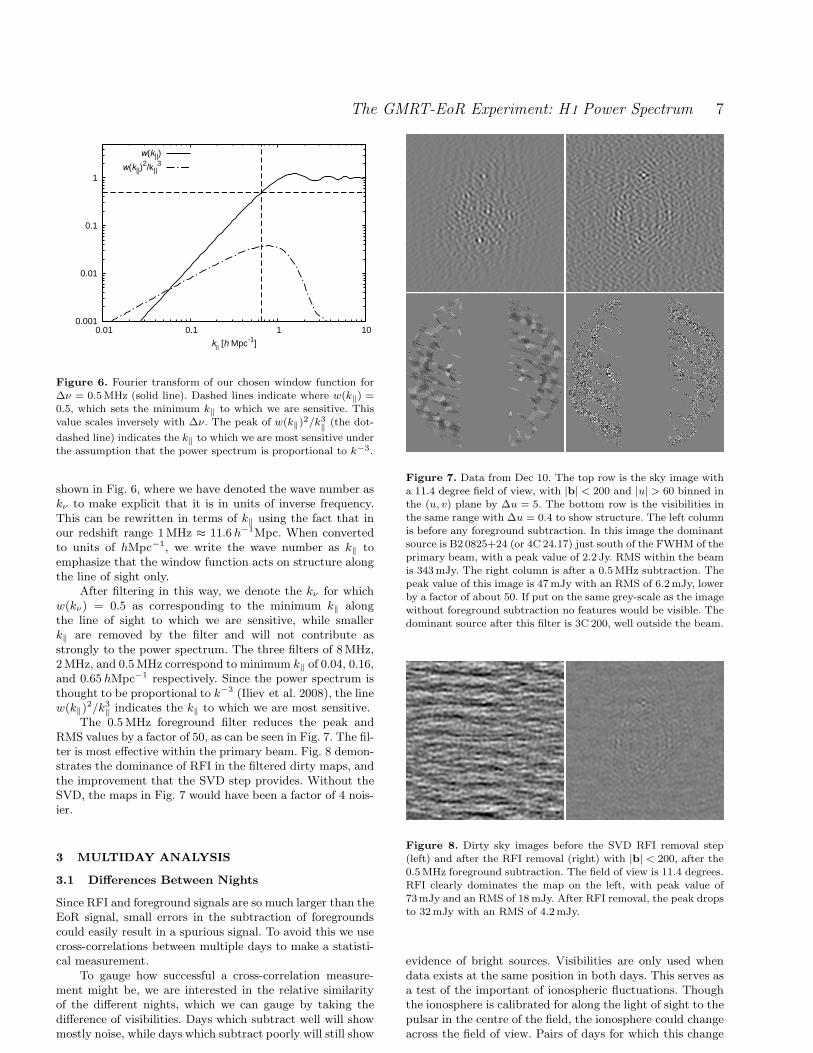
Figure 7. Data from Dec 10. The top row is the sky image witha 11.4 degree field of view, with |b| < 200 and |u| > 60 binned inthe (u, v) plane by ∆u = 5. The bottom row is the visibilities inthe same range with ∆u = 0.4 to show structure. The left columnis before any foreground subtraction. In this image the dominantsource is B2 0825+24 (or 4C 24.17) just south of the FWHM of theprimary beam, with a peak value of 2.2 Jy. RMS within the beamis 343mJy. The right column is after a 0.5MHz subtraction. Thepeak value of this image is 47mJy with an RMS of 6.2mJy, lowerby a factor of about 50. If put on the same grey-scale as the imagewithout foreground subtraction no features would be visible. Thedominant source after this filter is 3C 200, well outside the beam.

Figure 8. Dirty sky images before the SVD RFI removal step(left) and after the RFI removal (right) with |b| < 200, after the0.5MHz foreground subtraction. The field of view is 11.4 degrees.RFI clearly dominates the map on the left, with peak value of73mJy and an RMS of 18mJy. After RFI removal, the peak dropsto 32mJy with an RMS of 4.2mJy.

evidence of bright sources. Visibilities are only used whendata exists at the same position in both days. This serves asa test of the important of ionospheric fluctuations. Thoughthe ionosphere is calibrated for along the light of sight to thepulsar in the centre of the field, the ionosphere could changeacross the field of view. Pairs of days for which this change

c© 0000 RAS, MNRAS 000, 000–000

8 G. Paciga et al.

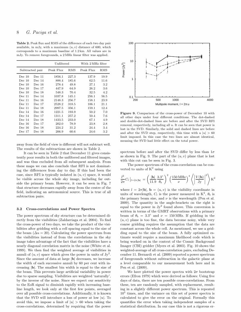
Table 2. Peak flux and RMS of the difference of each two day pairavailable, in mJy, with a maximum (u, v) distance of 600, whichcorresponds to a maximum baseline of 1.2 km. All values are inmJy. To remove foregrounds, a 2MHz linear filter was applied.

Unfiltered With 2MHz filter

Subtracted pair Peak Flux RMS Peak Flux RMS

Dec 10 Dec 11 1856.1 227.3 137.9 19.9Dec 10 Dec 14 888.4 185.6 62.5 11.6Dec 10 Dec 16 278.4 49.8 27.1 3.2Dec 10 Dec 17 447.9 64.9 26.2 3.6Dec 10 Dec 18 548.3 70.4 32.5 4.2Dec 11 Dec 14 1037.8 145.1 256.1 56.5Dec 11 Dec 16 2148.3 256.7 158.1 23.9Dec 11 Dec 17 2528.2 318.5 106.1 21.1Dec 11 Dec 18 2997.5 356.1 159.1 12.4Dec 14 Dec 16 1221.5 193.9 50.2 7.0Dec 14 Dec 17 1311.1 257.2 50.4 7.6Dec 14 Dec 18 1433.5 233.0 67.1 4.9Dec 16 Dec 17 202.0 78.9 23.8 2.8Dec 16 Dec 18 224.2 31.2 24.4 3.4Dec 17 Dec 18 206.9 60.6 24.6 3.2

away from the field of view is different will not subtract well.The results of the subtractions are shown in Table 2.

It can be seen in Table 2 that December 11 gives consis-tently poor results in both the unfiltered and filtered images,and was thus excluded from all subsequent analysis. Fromthese maps we can also conclude that RFI is not dominat-ing the differences from day to day. If this had been thecase, since RFI is typically isolated in (u, v) space, it wouldbe visible across the whole sky image, including far out-side the primary beam. However, it can be seen in Fig. 7that structure decreases rapidly away from the centre of thefield, indicating an astronomical source. This is true of allsubtraction pairs.

3.2 Cross-correlations and Power Spectra

The power spectrum of sky structure can be determined di-rectly from the visibilities (Zaldarriaga et al. 2004). To findthe cross-power of two days, we take the product of the visi-bilities after gridding with a cell spacing equal to the size ofthe beam (∆u = 20). Calculating the power spectrum fromthe visibilities instead of from the correlations in the skyimage takes advantage of the fact that the visibilities have anearly diagonal correlation matrix in the noise (White et al.1999). We then find the weighted average of visibilities inannuli of (u, v) space which gives the power in units of Jy2.Since the amount of data at large |b| decreases, we increasethe width of each successive annuli by 60 per cent with in-creasing |b|. The smallest bin width is equal to the size ofthe beam. This prevents large artificial variability in powerdue to sparse sampling. Visibilities are weighted ‘naturally’,by the inverse of the noise. Since we expect our sensitivityto the EoR signal to diminish rapidly with increasing base-line length, we look only at the first few points, averagedover all possible cross-correlations. Additionally, it is knownthat the SVD will introduce a loss of power at low |u|. Toavoid this, we impose a limit of |u| > 60 when taking thecross-correlations, determined by requiring that the power

0.1

1

10

100

200 500 1000 4000

Pow

er [J

y2 ]

Multipole moment, l = 2π u

Figure 9. Comparison of the cross-power of December 10 withall other days under four different conditions. The dot-dashedand double-dot-dashed lines are before and after the SVD RFIremoval, respectively, including all u. It can be seen that power islost in the SVD. Similarly, the solid and dashed lines are beforeand after the SVD step, respectively, this time with a |u| > 60limit imposed. In this case the two lines are almost identical,meaning the SVD had little effect on the total power.

spectrum before and after the SVD differ by less than 1σas shown in Fig. 9. The part of the (u, v) plane that is lostwith this cut can be seen in Fig. 3.

The power spectrum of the cross-correlation can be con-verted to units of K2 using

l2

2πCl

∣

∣

l=2π|b| =

(

|b|

11.9

3.3◦

θb

)2(

150MHz

ν

)4

⟨

∣

∣

∣

∣

V (b)

Jy

∣

∣

∣

∣

2⟩

K2

where l = 2π|b|, b = (u, v) is the visibility coordinate inunits of wavelength, Cl is the power measured in K2, θb isthe primary beam size, and ν is the wavelength (Pen et al.2009). The quantity in the angle-brackets on the right isequal to the power in Jy2 found above. This conversion iswritten in terms of the GMRT observations with a primarybeam of θb = 3.3◦ and ν = 150MHz. If gridding in the(u, v) plane is too fine, the data become noisy, while verycoarse gridding requires the assumption that the data areconstant across the whole cell. As mentioned, we use a grid-ding equal to the size of the beam. A fully optimized es-timate would require a maximum likelihood code which isbeing worked on in the context of the Cosmic BackgroundImager (CBI) gridder (Myers et al. 2003). Fig. 10 shows theweighted-average of all cross-correlation pairs, excluding De-cember 11. Bernardi et al. (2009) reported a power spectrumof foregrounds without subtraction in the galactic plane ata level comparable to our measurement both here and inPen et al. (2009).

We have plotted the power spectra with 2σ bootstraperrors (Efron 1979) which were derived as follows: Using fivedays of data, there are ten possible cross-correlations. Fromthese, ten are randomly sampled, with replacement, result-ing in a slightly different power spectrum. This is repeated104 times, and the variance on this set of power spectra iscalculated to give the error on the original. Formally thisquantifies the error when taking independent samples of astatistical distribution. In our case this is not a rigorous er-

c© 0000 RAS, MNRAS 000, 000–000

The GMRT-EoR Experiment: H I Power Spectrum 9

10-4

10-2

100

102

104

400 600 800 1000 1200 1400

l2 Cl /

2 π

[K2 ]

Multipole moment, l = 2π u

Figure 10. Average power spectrum in units of K2 of all com-binations of days, excluding December 11, as a function of themultipole moment l. Each point is shown with a 2σ upper limitderived from a bootstrap error analysis, which is in most casessmaller than the size of the point. The points are logarithmicallyspaced as described in the text, from left to right covering theranges 377 < l < 578, 578 < l < 899, and 899 < l < 1414. Tri-angles are the power before subtracting foregrounds, diamondsare after 8MHz mean subtraction, squares are after 2MHz meansubtraction, and circles are after 0.5MHz subtraction. The curvedsolid line is the theoretical EoR signal from Jelic et al. (2008), andthe dashed line is the theoretical EoR signal with a cold absorbingIGM as described in the text.

ror, but a suitable straightforward estimate given the maincomplications discussed earlier.

3.3 Comparison to Models

Fig. 10 can be compared to simulated results from theLow Frequency Array (LOFAR) EoR project in Jelic et al.(2008), which assumes Ts ≫ TCMB. At low l, their simu-lated EoR signal is approximately (10mK)2, while our low-est point with a similar 0.5MHz bandwidth filter is (50mK)2

with a 2σ upper limit of (70mK)2. These results are com-parable to the sensitivities LOFAR expects after 400 hoursof the EoR project. We have also considered the case wherereheating of the IGM does not occur, so the spin temper-ature remains coupled to the kinetic temperature of thegas (Ciardi & Madau 2003). In this case, the IGM coolsadiabatically after decoupling from the CMB at z ≈ 150.The temperature fluctuations scale with (1 + TCMB/Ts),and the power scales with the same factor squared. UsingTk = TCMB(1 + z)/150 at z = 8.6, the power becomes ap-proximately 275 times larger. This line is shown in Fig. 10,and is comparable to the data. Scaling up the warm IGMpower spectrum from Iliev et al. (2008) or Jelic et al. (2008)in this way is a reasonable approximation to what the ex-pected signal in a cold IGM. For a more detailed studies ofthe signal in such an absorption regime, we point the readerto Baek et al. (2009) and Baek et al. (2010).

The power spectrum of reionization is intrinsically threedimensional (Morales & Hewitt 2004). The strongest con-straints on the 3D power spectrum for the ∆ν = 2 and0.5MHz foreground filter case are shown in Fig. 11. Thisuses k2 = k2

‖+k2

⊥, where k‖ is given by the windowing func-

10-6

10-5

10-4

10-3

10-2

10-1

100

101

0.1 0.5 1

(k3 /2

π2 ) P

(k)

[K2 ]

k [h Mpc-1]

Figure 11. 3D power spectrum for the same data shown inFig. 10, using k2 = k2

‖+ k2

⊥. This is dominated by k‖, so the

bin width in k⊥ does not influence the horizontal position of thelimits. The strongest constraints from the 2MHz and 0.5MHz fil-ters are shown (square and circle, respectively). Upper limits are2σ bootstrap errors. Three possible signals are shown. The dashedline is the prediction from Iliev et al. (2008) and the double-dot-dashed line is the same for a cold IGM. The solid line comes fromthe single-scale bubble model as described in the text for a coldIGM, using k = 2.5/R to show the maximum power at all k. Forthe two points shown, the bubble diametres which achieve this

maximum power are 27 and 7.4h−1Mpc respectively. Only the0.5MHz point imposes a limit on the diametre. For a warm IGMcase, this signal would be reduced by the same factor as in thetwo dashed lines.

tion of the filter and k⊥ = l/6 h−1Gpc. When comparingthis to the prediction from Iliev et al. (2008), one shouldnote that our windowing function will also reduce the pre-dicted signal by at most a factor of two.

We also consider an idealized case in which the ionizedbubbles during reionization are of uniform scale and non-overlapping. Then for a given k there will be a characteristicbubble radius R at which the power is maximized. By takingthe 3D Fourier transform of a perfectly ionized bubble, andrequiring that the universe is 50 per cent ionized, one canshow the power is given by

k3

2π2P (k) =

3T 2

b

2π(kR)3

[

cos kR

(kR)2−

sin kR

(kR)3

]2

(4)

and is maximized when kR ≈ 2.5. In this case,k3/(2π2)P (k) ≈ T 2

b/5, where Tb is the brightness tempera-ture ≈ 30mK in an X-ray heated IGM or almost -500mKin a cold absorbing IGM. This signal would be more thanan order of magnitude larger than the predictions by e.g.Iliev et al. (2008) or Jelic et al. (2008). In Fig. 11 we haveincluded the power spectrum from this model with k cho-sen to maximize the power in the range of interest. Thedata currently impose a limit on the size of bubbles in thissingle-scale model. Our upper limits with a 0.5MHz fore-ground subtraction rule out bubbles with diametres from2.2 to 12.4 h−1Mpc in the redshift range 8.1 < z < 9.2. Thecold IGM constraint is applicable even in the case of simula-tions, since only UV photons are included which themselvesdo not heat the IGM.

c© 0000 RAS, MNRAS 000, 000–000

10 G. Paciga et al.

4 CONCLUSION

The data analysis has been completed on six days from De-cember 2007 with a noise level of approximately 2mJy onmost nights. The SVD removal strategies for broadband RFIused lower noise by a factor of 4 in temperature, or 16 inpower, which flagging alone cannot achieve. We have alsotested for ionospheric variations and found that our pulsarcalibration is sufficient for dealing with these effects. AfterRFI removal and foreground subtraction, we have measureda power spectrum which represents a new upper limit on the21 cm brightness temperature fluctuations during the epochof reionization. These results can be used to constrain as-sumptions about the state of the IGM at these times, par-ticularly in the case of a Ly-α pumped, but cold, IGM.

The previous best limit on 21 cm signal at comparableredshift was by Bebbington (1986), who reported no fea-tures down to 5K at z = 8.4. Parsons et al. (2010) havereported a similar limit of about 5K using PAPER. Theupper limit we present here is approximately 70mK on thevariance in 21 cm brightness temperature at z = 8.6, almosttwo orders of magnitude better than these previous limits.Residual foreground contamination and RFI may still becontributing to this power, but the EoR signal can not belarger than this.

The analysis of additional observations of the B0823+26field made since 2007, containing approximately 2 timesmore data than has been treated in this work, is ongoing.We expect to continue to improve these results, and theplanned addition of a second field will strengthen this sta-tistical measurement. The dominant uncertainty source re-mains RFI and foreground modelling.

These results provide a first-look at the progress madeat GMRT in detecting EoR. The GMRT-EoR team has beencontinuing observations, most recently with an additional150 hours allocated in the summer of 2010. We continue toimprove both the system temperature of GMRT antennasand the RFI monitoring and removal strategies and expectto improve upon these results as the analysis of the newerdata progresses.

5 ACKNOWLEDGMENTS

We thank Chris Hirata for his contributions to the analysispipeline and a reading of the paper, and the anonymous re-viewer for many useful comments. We also thank the staff ofthe GMRT that made these observations possible. GMRTis run by the National Centre for Radio Astrophysics ofthe Tata Institute of Fundamental Research. The compu-tations were performed on CITA’s Sunnyvale clusters whichare funded by the Canada Foundation for Innovation, theOntario Innovation Trust, and the Ontario Research Fund.The work of UP is supported by the National Science andEngineering Research Council of Canada. The map imagein Fig. 4 is copyright by OpenStreetMap7 contributors andused under license8.

7 http://www.openstreetmap.org/8 http://creativecommons.org/licenses/by-sa/2.0/

REFERENCES

Alvarez M. A., Pen U., Chang T., 2010, ApJ, 723, L17Ananthakrishnan S., 1995, Journal of Astrophysics and As-tronomy Supplement, 16, 427

Baek S., Di Matteo P., Semelin B., Combes F., Revaz Y.,2009, A&A, 495, 389

Baek S., Semelin B., Di Matteo P., Revaz Y., Combes F.,2010, preprint (astro-ph/1003.0834)

Bebbington D. H. O., 1986, MNRAS, 218, 577Becker R. H. et al., 2001, AJ, 122, 2850

Bernardi G., de Bruyn A. G., Brentjens M. A., Ciardi B.,Harker G., Jelic V., Koopmans L. V. E., Labropoulos P.,Offringa A., Pandey V. N., Schaye J., Thomas R. M.,Yatawatta S., Zaroubi S., 2009, A&A, 500, 965

Bowman J. D., Morales M. F., Hewitt J. N., 2006, ApJ,638, 20

Bowman J. D., Morales M. F., Hewitt J. N., 2009, ApJ,695, 183

Chen X., Miralda-Escude J., 2004, ApJ, 602, 1Chuzhoy L., Shapiro P. R., 2006, ApJ, 651, 1

Ciardi B., Madau P., 2003, ApJ, 596, 1Cooray A., Li C., Melchiorri A., 2008, Phys. Rev. D, 77,103506

Cornwell T. J., Golap K., Bhatnagar S., 2008, IEEE Jour-nal of Selected Topics in Signal Processing, Vol. 2, Issue5, p.647-657, 2, 647

Dalal N., Pen U., Seljak U., 2010, preprint (astro-ph/1009.4704)

Datta A., Bowman J. D., Carilli C. L., 2010, ApJ, 724, 526

Di Matteo T., Ciardi B., Miniati F., 2004, MNRAS, 355,1053

Dijkstra M., Haiman Z., Loeb A., 2004, ApJ, 613, 646

Djorgovski S. G., Castro S., Stern D., Mahabal A. A., 2001,ApJ, 560, L5

Dunkley J., Komatsu E., Nolta M. R., Spergel D. N., Lar-son D., Hinshaw G., Page L., Bennett C. L., Gold B.,Jarosik N., Weiland J. L., Halpern M., Hill R. S., KogutA., Limon M., Meyer S. S., Tucker G. S., Wollack E.,Wright E. L., 2009, ApJS, 180, 306

Efron B., 1979, Ann. Statist., 7, 1Fan X., Narayanan V. K., Strauss M. A., White R. L.,Becker R. H., Pentericci L., Rix H., 2002, AJ, 123, 1247

Fan X., Strauss M. A., Becker R. H., White R. L., GunnJ. E., Knapp G. R., Richards G. T., Schneider D. P.,Brinkmann J., Fukugita M., 2006, AJ, 132, 117

Field G. B., 1959, ApJ, 129, 536Furlanetto S. R. et al, 2009, in astro2010: The Astronomyand Astrophysics Decadal Survey Vol. 2010 of Astronomy,Cosmology from the Highly-Redshifted 21 cm Line. pp82–+

Furlanetto S. R., Oh S. P., Briggs F. H., 2006, Phys. Rep.,433, 181

Furlanetto S. R., Zaldarriaga M., Hernquist L., 2004, ApJ,613, 1

Gunn J. E., Peterson B. A., 1965, ApJ, 142, 1633Guo Q., Wu X., Xu H. G., Gu J. H., 2009, ApJ, 693, 1000

Harker G., Zaroubi S., Bernardi G., Brentjens M. A., deBruyn A. G., Ciardi B., Jelic V., Koopmans L. V. E.,Labropoulos P., Mellema G., Offringa A., Pandey V. N.,Pawlik A. H., Schaye J., Thomas R. M., Yatawatta S.,2010, MNRAS, 405, 2492

c© 0000 RAS, MNRAS 000, 000–000

The GMRT-EoR Experiment: H I Power Spectrum 11

Harker G., Zaroubi S., Bernardi G., Brentjens M. A., deBruyn A. G., Ciardi B., Jelic V., Koopmans L. V. E.,Labropoulos P., Mellema G., Offringa A., Pandey V. N.,Schaye J., Thomas R. M., Yatawatta S., 2009, MNRAS,397, 1138

Hobbs G., Lyne A. G., Kramer M., Martin C. E., JordanC., 2004, MNRAS, 353, 1311

Hobson M. P., Maisinger K., 2002, MNRAS, 334, 569Hogan C. J., Rees M. J., 1979, MNRAS, 188, 791Iliev I. T., Mellema G., Pen U., Merz H., Shapiro P. R.,Alvarez M. A., 2006, MNRAS, 369, 1625

Iliev I. T., Mellema G., Pen U.-L., Bond J. R., ShapiroP. R., 2008, MNRAS, 384, 863

Jelic V., Zaroubi S., Labropoulos P., Bernardi G., de BruynA. G., Koopmans L. V. E., 2010, MNRAS, pp 1369–+

Jelic V., Zaroubi S., Labropoulos P., Thomas R. M.,Bernardi G., Brentjens M. A., de Bruyn A. G., CiardiB., Harker G., Koopmans L. V. E., Pandey V. N., SchayeJ., Yatawatta S., 2008, MNRAS, 389, 1319

Kassim N. E., Lazio T. J. W., Ray P. S., Crane P. C.,Hicks B. C., Stewart K. P., Cohen A. S., Lane W. M.,2004, Planet. Space Sci., 52, 1343

Komatsu E., Smith K. M., Dunkley J., et al 2010, preprint(astro-ph/1001.4538)

Lidz A., Zahn O., McQuinn M., Zaldarriaga M., HernquistL., 2008, ApJ, 680, 962

Liu A., Tegmark M., Bowman J., Hewitt J., ZaldarriagaM., 2009, MNRAS, 398, 401

Liu A., Tegmark M., Zaldarriaga M., 2009, MNRAS, 394,1575

Loeb A., Zaldarriaga M., 2004, Phys. Rev. Lett., 92, 211301Lonsdale C. J. et al., 2009, IEEE Proceedings, 97, 1497Madau P., Meiksin A., Rees M. J., 1997, ApJ, 475, 429Mao Y., Tegmark M., McQuinn M., Zaldarriaga M., ZahnO., 2008, Phys. Rev. D, 78, 023529

Masui K. W., McDonald P., Pen U., 2010, Phys. Rev. D,81, 103527

McQuinn M., Lidz A., Zahn O., Dutta S., Hernquist L.,Zaldarriaga M., 2007, MNRAS, 377, 1043

McQuinn M., Zahn O., Zaldarriaga M., Hernquist L.,Furlanetto S. R., 2006, ApJ, 653, 815

Mezzacappa A., 2005, Annual Review of Nuclear and Par-ticle Science, 55, 467

Morales M. F., 2005, ApJ, 619, 678Morales M. F., Bowman J. D., Cappallo R., Hewitt J. N.,Lonsdale C. J., 2006, New Astronomy Review, 50, 173

Morales M. F., Bowman J. D., Hewitt J. N., 2006, ApJ,648, 767

Morales M. F., Hewitt J., 2004, ApJ, 615, 7Morales M. F., Wyithe J. S. B., 2010, ARA&A, 48, 127Myers S. T., Contaldi C. R., Bond J. R., Pen U., PogosyanD., Prunet S., Sievers J. L., Mason B. S., Pearson T. J.,Readhead A. C. S., Shepherd M. C., 2003, ApJ, 591, 575

Parsons A. R., Backer D. C., Foster G. S., Wright M. C. H.,Bradley R. F., Gugliucci N. E., Parashare C. R., BenoitE. E., Aguirre J. E., Jacobs D. C., Carilli C. L., Herne D.,Lynch M. J., Manley J. R., Werthimer D. J., 2010, AJ,139, 1468

Pearson T. J., Kus A. J., 1978, MNRAS, 182, 273Pen U., Chang T., Hirata C. M., Peterson J. B., Roy J.,Gupta Y., Odegova J., Sigurdson K., 2009, MNRAS, 399,181

Peterson J., Pen U., Wu X., 2004, preprint (astro-ph/0404083)

Pritchard J. R., Loeb A., 2010, Phys. Rev. D, 82, 023006Purcell E. M., Field G. B., 1956, ApJ, 124, 542Rottgering H. J. A. et al., 2006, preprint (astro-ph/0610596)

Roy J., Gupta Y., Pen U., Peterson J. B., Kudale S.,Kodilkar J., 2010, Experimental Astronomy, 28, 25

Salvaterra R., Haardt F., Volonteri M., 2007, MNRAS, 374,761

Scott D., Rees M. J., 1990, MNRAS, 247, 510Shapiro P. R., Ahn K., Alvarez M. A., Iliev I. T., MartelH., Ryu D., 2006, ApJ, 646, 681

Sunyaev R. A., Zeldovich I. B., 1975, MNRAS, 171, 375Thompson A. R., Moran J. M., Swenson Jr. G. W., 2001,Interferometry and Synthesis in Radio Astronomy, 2ndEdition

Trac H., Gnedin N. Y., 2009, preprint (astro-ph/0906.4348)Tseliakhovich D., Hirata C., 2010, preprint (astro-ph/1005.2416)

Wang X., Tegmark M., Santos M. G., Knox L., 2006, ApJ,650, 529

White M., Carlstrom J. E., Dragovan M., Holzapfel W. L.,1999, ApJ, 514, 12

Willis A. G., Oosterbaan C. E., de Ruiter H. R., 1976,A&AS, 25, 453

Willott C. J., Delorme P., Omont A., Bergeron J., DelfosseX., Forveille T., Albert L., Reyle C., Hill G. J., Gully-Santiago M., Vinten P., Crampton D., Hutchings J. B.,Schade D., Simard L., Sawicki M., Beelen A., Cox P., 2007,AJ, 134, 2435

Willott C. J., Rawlings S., Blundell K. M., 2001, MNRAS,324, 1

Wouthuysen S. A., 1952, AJ, 57, 31Zahn O., Lidz A., McQuinn M., Dutta S. a., 2007, ApJ,654, 12

Zaldarriaga M., Furlanetto S. R., Hernquist L., 2004, ApJ,608, 622

Zaroubi S., Silk J., 2005, MNRAS, 360, L64

c© 0000 RAS, MNRAS 000, 000–000