Momentum has its Moments�

Pedro Barrosoy and Pedro Santa-Claraz

First version: April 2012This version: April 2013

Abstract

Compared to the market, value or size factors, momentum has o¤ered

investors the highest Sharpe ratio. However, momentum has also had the

worst crashes, making the strategy unappealing to investors with reasonable

risk aversion. We �nd that the risk of momentum is highly variable over time

and quite predictable. The major source of predictability is not time-varying

market risk but rather momentum-speci�c risk. Managing this risk virtually

eliminates crashes and nearly doubles the Sharpe ratio of the momentum

strategy. Risk management works because high risk forecasts both high risk

and low returns. As a result, risk-managed momentum is a much greater

puzzle than the original version.

�We thank Abhay Abhyankar, Eduardo Schwartz, David Lando, Denis Chaves, James Sefton,José Filipe Corrêa Guedes, Kent Daniel, Kristian Miltersen, Lasse Pederson, Nigel Barradale,Pasquale Della Corte, Richard Harris, Robert Kosowski, Soeren Hvidkjaer and numerous seminarparticipants at BI Norwegian School of Business, Copenhagen Business School, CUNEF, ImperialCollege, Nova School of Business and Economics, Universidad Carlos III and University of Exeterfor their helpful comments and suggestions. A previous version of this paper circulated with thetitle �Managing the Risk of Momentum�. Santa-Clara is supported by a grant from the Fundaçãopara a Ciência e Tecnologia (PTDC/EGE-GES/101414/2008).

yNova School of Business and Economics. E-mail: pmsb@novasbe.pt.zMillennium Chair in Finance. Nova School of Business and Economics and NBER and

CEPR. E-mail: psc@novasbe.pt.

1

1 Introduction

Momentum is a pervasive anomaly in asset prices. Jegadeesh and Titman (1993)

�nd that previous winners in the US stock market outperform previous losers by

as much as 1.49 percent a month. The Sharpe ratio of this strategy exceeds the

Sharpe ratio of the market itself, as well as the size and value factors. Momentum

returns are even more of a puzzle since they are negatively correlated to those of the

market and value factors. Indeed, from 1927 to 2011, momentum had a monthly

excess return of 1.75 percent controlling for the Fama-French factors.1 Moreover,

momentum is not just a US stock market anomaly. Momentum has been docu-

mented in European equities, emerging markets, country stock indices, industry

portfolios, currency markets, commodities and across asset classes.2 Grinblatt and

Titman (1989,1993) �nd most mutual fund managers incorporate momentum of

some sort in their investment decisions, so relative strength strategies are wide-

spread among practitioners.

But the remarkable performance of momentum comes with occasional large

crashes.3 In 1932, the winners-minus-losers strategy delivered a -91.59 percent

return in just two months. In 2009, momentum experienced a crash of -73.42

percent in three months. Even the large returns of momentum do not compensate

an investor with reasonable risk aversion for these sudden crashes that take decades

to recover from.

The two most expressive momentum crashes occurred as the market rebounded

following large previous declines. One explanation for this pattern is the time-

varying systematic risk of the momentum strategy. Grundy and Martin (2001)

show that momentum has signi�cant negative beta following bear markets.4 They

argue that hedging this time-varying market exposure produces stable momentum

1This result has led researchers to use momentum as an additional risk factor � Carhart(1997).

2See Rouwenhorst (1998,1999) for international evidence, Asness, Liew, and Stevens (1997)for country stock indices, Moskowitz and Grinblatt (1999) for industry portfolios, Okunev andWhite (2003) and Menkhof, Sarno, Schmeling, and Schrimpf (2012) for currency markets, Erband Harvey (2006) for commodities and Asness, Moskowitz, and Pederson (2011) for momentumacross asset classes.

3Daniel and Moskowitz (2011)4Following negative returns for the overall market, winners tend to be low-beta stocks and

the reverse for losers. Therefore the winner-minus-losers strategy will have a negative beta.

2

returns but Daniel and Moskowitz (2012) show that using betas in real time does

not avoid the crashes.

In this work we propose a di¤erent method to manage the risk of the momentum

strategy. We estimate the risk of momentum by the realized variance of daily

returns and �nd that it is highly predictable. An auto-regression of monthly

realized variances yields an out-of-sample (OOS) R-square of 57.82 percent. This

is 19.01 percentage points (p.p.) higher than a similar auto-regression for the

variance of the market portfolio which is already famously predictable.5

Furthermore, we �nd that high risk also forecasts lower momentum returns. In

the years after a period of low realized volatility, the return of momentum is on

average 24.35 percent. This contrasts with 0.96 percent in the years following a

period of high realized volatility. The strategy delivers higher return when it is less

risky, a clearly counter intuitive result that challenges any risk-based explanation

for the strategy�s performance.

Managing the risk of momentum leads to substantial economic gains. We sim-

ply scale the long-short portfolio by its realized volatility in the previous 6 months,

targeting a strategy with constant volatility.6 The Sharpe ratio improves from 0.53

for unmanaged momentum to 0.97 for its risk-managed version. But the most im-

portant bene�t comes from a reduction in crash risk. The excess kurtosis drops

from 18.24 to 2.68 and the left skew improves from -2.47 to -0.42. The minimum

one-month return for raw momentum is -78.96 percent while for risk-managed mo-

mentum is -28.40 percent. The maximum drawdown of raw momentum is -96.69

percent versus -45.20 percent for its risk-managed version.

To assess the economic signi�cance of our results, we evaluate the bene�ts of

risk management for a risk-averse investor with a one-year horizon using a power

utility function with Constant Relative Risk Aversion (CRRA) of four. Holding

the market portfolio has an annual certainty equivalent of 0.14 percent to this

investor. Adding momentum to the portfolio reduces the certainty equivalent to

-5.46 percent. However, combining the market with risk-managed momentum

achieves a certainty equivalent of 13.54 percent. We �nd that the main bene�t of

5Engle and Bollerslev (1986), Schwert (1989).6This aproach only relies on past data and thus does not su¤er from look-ahead bias. Scaling

the portfolio to have constant volatility over time is actually a more natural way of implementingthe strategy than having a constant amount long and short with varying volatility.

3

risk management comes in the form of lower crash risk. This alone provides a gain

of 14.96 p.p. in annual certainty equivalent.

The performance of scaled momentum is robust in sub-samples and in interna-

tional data. Using overlapping 10-year periods, we show that managing the risk

of momentum not only avoids its worse crashes but it also improves the Sharpe

ratio in 97.66 percent of the 10-year periods. Besides the US, risk-management

also improves the Sharpe ratio of momentum in all the major markets we examine

(France, Germany, Japan, and the UK).

One pertinent question is why managing risk with realized variances works

while using time-varying betas does not. To answer this question we decompose

the risk of momentum into market risk (from time-varying exposure to the market)

and speci�c risk. We �nd that the market component is only 23 percent of total

risk on average, so most of the risk of momentum is speci�c to the strategy.7 This

speci�c risk is more persistent and predictable than the market component. The

OOS R-square of predicting the speci�c component is 47 percent versus 21 percent

for the systematic component. This is why hedging with time-varying betas fails:

it focuses on the smaller and less predictable part of risk.

The research that is most closely related to ours is Grundy and Martin (2001)

and Daniel and Moskowitz (2012). But their work studies the time-varying sys-

tematic risk of momentum, while we focus on momentum�s speci�c risk. Our

results have the distinct advantage of o¤ering investors using momentum strate-

gies an e¤ective way to manage risk without forward-looking bias. The resulting

risk-managed strategy deepens the puzzle of momentum.

After the dismal performance of momentum in the last ten years, some could

argue it is a dead anomaly. Our results indicate that momentum is not dead. It just

so happens that the last ten years were rich in the kind of high-risk episodes that

lead to bad momentum performance. Our paper is related to the recent literature

that proposes alternative versions of momentum. Blitz, Huij and Martens (2011)

show that sorting stocks according to their past residuals rather than gross returns

produces a more stable version of momentum. Chaves (2012) shows that most of

7By momentum-speci�c risk we do not mean �rm-speci�c risk or idiosyncratic risk. Momen-tum is a well diversi�ed portfolio and all its risk is systematic. It just happens that a largeportion of the risk of momnetum is not explained by other risk factors.

4

the bene�t in that method comes from using the market model in the regression

and extends the evidence for residual momentum internationally.

Our work is also related to the literature on whether risk factors explain the

risk of momentum (Gri¢ n, Ji, and Martin (2003), Cooper, Gutierrez, and Hameed

(2004), Fama and French (2012)).

This paper is structured as follows. Section 2 discusses the long-run properties

of momentum returns and its exposure to crashes. Section 3 shows that momentum

risk varies substantially over time in a highly predictable manner. Section 4 shows

there is no risk-return trade-o¤ for momentum. Actually we �nd the opposite

of a trade-o¤. We analyze the implications of the predictability in momentum

risk and return in Section 5. In Section 6 we use an utility based approach to

decompose the gains of risk management according to the moments of returns.

In Section 7 we decompose the risk of momentum and study the persistence of

each of its components separately. In section 8 we check if our �ndings also hold

internationally. In section 9 we assess the robustness of our �ndings across sub-

samples. Finally, Section 10 presents our conclusions.

2 Momentum in the long run

We compare momentum to the Fama-French factors using a long sample of 85

years of monthly returns from July 1926 to December 2011.8 This is the same

sample period as in Daniel and Moskowitz (2012).

Figure 1 presents the cumulative returns of each factor. As each factor consists

of a long-short strategy, we construct the series of returns assuming the investor

puts $1 in the risk-free asset at the beginning of the sample, buys $1 worth of

the long portfolio and sells the same amount of the short portfolio. Then, in

each subsequent month, the strategy fully reinvests the accumulated wealth in the

risk-free asset, assuming a position of the same size in the long and short legs

of the portfolio. The winners-minus-losers (WML) strategy o¤ered an impressive

performance for investors. One dollar fully reinvested in the momentum strategy

grew to $68,741 by the end of the sample. This compares to the cumulative return

8See the appendix for a description of the data.

5

of $2,136 from simply holding the market portfolio. Table 1 compares descriptive

statistics for momentum in the long run with the Fama-French factors. Buying

winners and shorting losers has provided large returns of 14.46 percent per year,

with a Sharpe ratio higher than the market.

There would be nothing puzzling about momentum�s returns if they corre-

sponded to a very high exposure to risk. However, running an OLS regression of

the WML on the Fama-French factors gives (t-stats in parenthesis):

rWML;t = 1:752 �0:378 rRMRF;t �0:249 rSMB;t �0:677 rHML;t

(7:93) (�8:72) (�3:58) (�10:76)(1)

so momentum provided abnormal returns of 1.75 percent per month after control-

ling for its negative exposure to the Fama and French (1992) risk factors. This

amounts to a 21 percent per year abnormal return and the negative loadings on

the risk factors imply momentum actually diversi�ed risk in this extended sample.

The impressive excess returns of momentum, its high Sharpe ratio and negative

relation to other risk factors, particularly the value premium, make it look like a

free lunch to investors. But as Daniel and Moskowitz (2012) show there is a

dark side to momentum. Its large gains come at the expense of a very high excess

kurtosis of 18.24 combined with a pronounced left-skew of -2.47. These two features

of the distribution of returns of the momentum strategy imply a very fat left tail

�signi�cant crash risk. Momentum returns can very rapidly turn into a free fall,

wiping out decades of returns.

Figure 2 shows the performance of momentum in the two most turbulent

decades for the strategy: the 1930�s and the 2000�s. In July and August 1932,

momentum had a cumulative return of -91.59 percent. From March to May 2009,

momentum had another large crash of -73.42 percent. These short periods had

an enduring impact on cumulative returns. For example, someone investing one

dollar in the WML strategy in July 1932 would only recover it in April 1963, 31

years later and with considerably less real value. This puts the risk to momentum

investing in an adequate long-run perspective.

Both in 1932 and in 2009, the crashes happened as the market rebounded

6

after experiencing large losses.9 This leads to the question of whether investors

could have predicted the crashes in real time and hedge them away. Grundy

and Martin (2001) show that momentum has a substantial time-varying loading

on stock market risk. The strategy ranks stocks according to returns during a

formation period, for example the previous 12 months. When the stock market

performed well in the formation period, winners tend to be high-beta stocks and

losers low-beta stocks. So the momentum strategy, by shorting losers to buy

winners, has by construction a signi�cant time-varying beta: positive after bull

markets and negative after bear markets. They argue that hedging this time-

varying risk produces stable returns, even in pre-WWII data, when momentum

performed poorly. In particular, the hedging strategy would be long in the market

portfolio whenever momentum has negative betas, hence mitigating the e¤ects of

rebounds following bear markets, which is when momentum experiences the worst

returns. But the hedging strategy in Grundy and Martin (2001) uses forward

looking betas, estimated with information investors did not have in real time.

Using betas estimated solely on ex-ante information does not avoid the crashes

and portfolios hedged in real time often perform even worse than the original

momentum strategy (Daniel and Moskowitz (2012), Barroso (2012)).

3 The time-varying risk of momentum

One possible cause for excess kurtosis is time-varying risk.10 The very high excess

kurtosis of 18.24 of the momentum strategy (more than twice the market portfolio)

leads us to study the dynamics of its risk and compare it with the risk of the market

(RMRF), value (HML) and size (SMB) risk factors.

For each month, we compute the realized variance RVt from daily returns in

the previous 21 sessions. Let frdgDd=1 be the daily returns and fdtgTt=1 the timeseries of the dates of the last trading sessions of each month. Then the realized

variance of factor i in month t is:11

9Daniel and Moskowitz (2011) argue this is due to the option-like payo¤s of distressed �rmsin bear markets.10See, for example, Engle (1982) and Bollerslev (1987).11Correcting for serial correlation of daily returns does not change the results signi�cantly.

7

RVi;t =20Xj=0

r2i;dt�j (2)

Figure 3 shows the monthly realized volatility of momentum. This varies substan-

tially over time, from a minimum of 3.04 percent (annualized) to a maximum of

127.87 percent.

Table 2 shows the results of AR (1) regressions of the realized variances of the

WML, RMRF, SMB and HML:

RVi;t = �+ �RVi;t�1 + "t (3)

Panel A presents the results for RMRF and WML, for which we have daily

data available from 1927:03 to 2011:12. Panel B adds the results for HML and

SMB, for which daily data is available only from 1963:07 onwards.

Momentum returns are the most volatile. From 1927:03 to 2011:12, the average

realized volatility of momentum is 15.03, more than the 12.81 of the market port-

folio. For 1963:07 onwards, the average realized volatility of momentum is 16.40,

also the highest when compared to RMRF, SMB and HML.

In the full sample period, the standard deviation of monthly realized volatilities

is higher for momentum (12.26) than the market (7.82). Panel B con�rms this

result compared to the other factors in the 1963:07 onwards sample. So the risk

of momentum is the most variable.

The risk of momentum is also the most persistent. The AR(1) coe¢ cient of

the realized variance of momentum in the 1963:07 sample is 0.77, which is 0.19

more than for the market and higher than the estimates for SMB and HML.

To check the out-of-sample (OOS) predictability of risk, we use a training sam-

ple of 240 months to run an initial AR(1) and then use the estimated coe¢ cients

and last observation of realized variance to forecast the realized variance in the

following month. Then each month we use an expanding window of observations to

produce OOS forecasts and compare these to the accuracy of the historical mean

RV i;t. As a measure of goodness of �t we estimate the OOS R-square as:

8

R2i;OOS = 1�

T�1Pt=S

(b�t + b�tRVi;t �RVi;t+1)2T�1Pt=S

(RV i;t �RVi;t+1)2(4)

where S is the initial training sample, b�t;b�t and RV i;t are estimated with informa-tion available only up to time t.

The last column of table 2 shows the OOS R-squares of each auto-regression.

The AR(1) of the realized variance of momentum has an OOS R-square of 57.82

percent (full sample), which is 50 percent more than the market. For the period

from 1963:07 to 2011:12, the OOS predictability of momentum risk is twice that

of the market. Hence more than half of the risk of momentum is predictable, the

highest level among risk factors.

4 No risk-return trade-o¤ in momentum

Predictable risk does not necessarily imply the possibility of achieving economic

gains by managing risk. If higher risk also forecasts higher returns, the implicit

trade-o¤could leave investors indi¤erent. But in fact, we �nd exactly the opposite.

Higher risk in the momentum factor forecasts lower expected returns going forward.

A predictive regression of the monthly returns of momentum on lagged 6-month

realized variance holds (t-stats in parenthesis):rWML;t+1 = 1:79 �1:51 RVWML(�6);t

(6:46) (�4:63)The monthly returns are from 1927:03 to 2011:12. The regression has an R-

square of 2.06 percent, which is high for a predictive regression at monthly fre-

quency. Moreover, the OOS R-square, considering a training sample of 240 months,

is of 1.85 percent. So, unlike most predictive regressions for the market return

(Goyal and Welch (2008)), the regression is robust out of sample.12

Figure 4 illustrates the potential of realized variance of momentum to condition

exposure to the factor. We sort the months into quintiles according to the level

12Examining the two legs separately, we �nd the variance of momentum forecasts both higherreturns for the losers portfolio and lower returns for the winners portfolio. But predictability ismuch stronger for the winner-minus-losers portfolio.

9

of realized variance in the previous 6 months for each factor: the market and

momentum. Quintile 1 is the set of months with lowest risk and quintile 5 is

the one with highest risk. Then we report, for each factor, the average realized

volatility, return and Sharpe ratio in the following 12 months.

In general, higher risk in the recent past forecasts higher risk going forward.

This is true both for the market and the momentum factors, but more so in the

case of momentum.

For the market there is no obvious trade-o¤ between risk and return. This

illustrates the well-known di¢ culty in estimating this relation.13 But this is not

true for momentum. The winners-minus-losers portfolio has a very clear negative

relation between risk and return. In the years following calm periods (in quintile

1), the average annual return of the momentum strategy is 24.35%. By contrast,

in the years following a turbulent period (in quintile 5), the average return of the

momentum strategy is only 0.96%.

This negative relation between risk and return adds a new layer to the mo-

mentum puzzle. Higher risk forecasts both higher risk and lower returns. As a

consequence the Sharpe ratio of the momentum factor changes considerably con-

ditional on its previous risk. In the years after a calm period, the Sharpe ratio

is 1.72 on average. By contrast, after a turbulent period the Sharpe ratio is only

0.28 on average.

In the next section, we explore the combined potential of this predictability

in returns with the predictability of risk and show their usefulness to manage the

exposure to momentum.

5 Risk-managed momentum

We use an estimate of momentum risk to scale the exposure to the strategy in

order to have constant risk over time.14 For each month we compute a variance

13See, for example, Glosten et al. (1993), Ghysels et al. (2005).14Volatility-scaling has been used in the time series momentum literature (Moskowitz, Ooi,

and Pederson (2012) and Baltas and Kosowski (2013)). But there it serves a di¤erent purpose:use the asset-speci�c volatility to prevent the results from being dominated by high-volatilityassets only. We do not consider asset-speci�c volatilities and actually show that the persistencein risk of the winners-minus-losers strategy is more interesting than that of a long-only portfolio

10

forecast �̂2t from daily returns in the previous 6 months.15 Let frWML;tgTt=1 be the

monthly returns of momentum and frWML;dgDd=1; fdtgTt=1 be, as above, the dailyreturns and the time series of the dates of the last trading sessions of each month.

The variance forecast is:

�̂2WML;t = 21125Xj=0

r2WML;dt�1�j=126 (5)

As WML is a zero-investment and self-�nancing strategy we can scale it with-

out constraints. We use the forecasted variance to scale the returns:

rWML�;t =�target�̂t

rWML;t (6)

where rWML;t is the unscaled or plain momentum, rWML�;t is the scaled or risk-

managed momentum, and �target is a constant corresponding to the target level

of volatility. Scaling corresponds to having a weight in the long and short legs

that is di¤erent from one and varies over time, but it keeping the strategy still

self-�nancing. We pick a target corresponding to an annualized volatility of 12

percent.16

Figure 5 shows the cumulative returns of risk-managed momentum compared

to plain momentum. The risk-managed momentum strategy achieves a higher

cumulative return with less risk. So there are economic gains to risk management

of momentum. The scaled strategy bene�ts from the large momentum returns

when it performs well and e¤ectively shuts o¤ in turbulent times, thus mitigating

momentum crashes. As a result, one dollar invested in risk-managed momentum

grows to $6,140,075 by the end of the sample, nearly 90 times more than the plain

momentum strategy.17 Also, the risk-managed strategy no longer has variable and

of assets, such as the market.15We also used one-month and three-month realized variances as well as exponentially-weighted

moving average (EWMA) with half-lifes of 1, 3 and 6 months. All work well with nearly identicalresults.16The annualized standard deviation from monthly returns will be higher than 12% as volatil-

ities at daily frequency are not directly comparable to those at lower frequencies due to the smallpositive autocorrelation of daily returns.17This di¤erence in cumulative returns is fundamentally due to risk management successfully

avoiding the two momentum crashes. But in the post-war period from 1946 to 2007, not includingthe crashes, the Sharpe ratio of momentum was 0.86, versus 1.15 for risk-managed momentum.

11

persistent risk, so risk management does indeed work.18

Table 3 provides a summary of the economic performance of WML� in 1927-

2011. The risk-managed strategy has a higher average return, with a gain of 2.04

percentage points per year, with substantially less standard deviation (less 10.58

percentage points per year). As a result, the Sharpe ratio of the risk-managed

strategy almost doubles from 0.53 to 0.97. The most important gains of risk-

management show up in the improvement in the higher order moments. Managing

the risk of momentum lowers the excess kurtosis from a very high value of 18.24 to

just 2.68 and reduces the left skew from -2.47 to -0.42. This practically eliminates

the crash risk of momentum. Figure 6 shows the density function of momentum

and its risk-managed version. Momentum has a very long left tail which is much

reduced in its risk-managed version.

The bene�ts of risk-management are especially important in turbulent times.

Figure 7 shows the performance of risk-managed momentum in the decades with

the most impressive crashes. The scaled momentum manages to preserve the

investment in the 1930�s. This compares very favorably to the pure momentum

strategy which loses 90 percent in the same period. In the 2000�s simple momentum

loses 28 percent of wealth, because of the crash in 2009. Risk-managed momentum

ends the decade up 88 percent as it not only avoids the crash but also captures

part of the positive returns of 2007-2008.

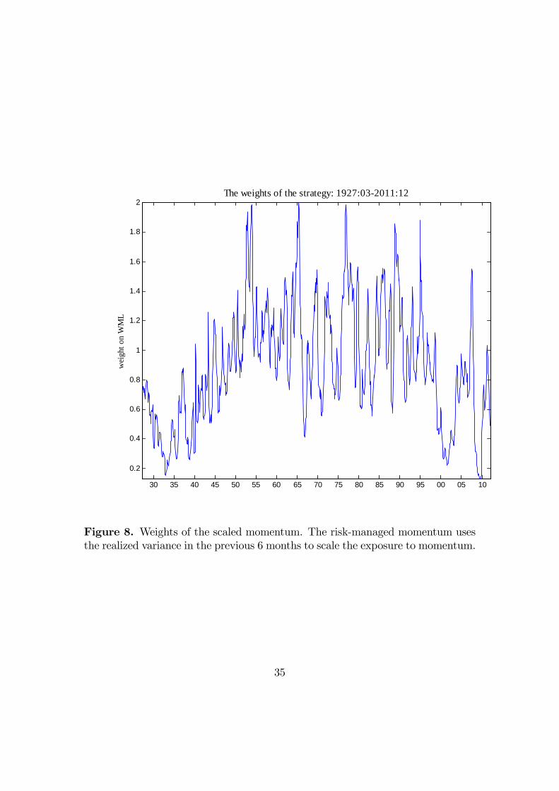
Figure 8 shows the weights of the scaled momentum strategy over time �in-

terpreted as the dollar amount in the long or short leg. These range between the

values of 0.13 and 2.00, reaching the most signi�cant lows in the early 1930�s, in

2000-02, and in 2008-09. On average, the weight is 0.90, slightly less than full

exposure to momentum. As these weights depend only on ex-ante information

this strategy could actually be implemented in real time. Actually, running a

long-short strategy to have constant volatility is closer to what real investors (like

hedge funds) try to do than keeping a constant amount invested in the long and

short legs of the strategy.

So risk management also contributes to performance in less turbulent times.18The AR(1) coe¢ cient of monthly squared returns is only 0.14 for the scaled momentum versus

0.40 for the original momentum. Besides, the auto-correlation of raw momentum is signi�cant upto 15 lags while only 1 lag for risk-managed momentum. So persistence in risk is much smallerfor the risk-managed strategy.

12

6 Economic signi�cance: An investor perspec-

tive

Raw momentum o¤ers a trade-o¤ between an appealing Sharpe ratio, obtained

from the �rst two moments of its distribution, and less appealing higher order mo-

ments, such as high kurtosis and left skewness. An economic criterion is needed to

assess whether this trade-o¤ is interesting. Risk management o¤ers improvements

to momentum across the board, higher expected returns, lower standard deviation

and crash risk. Still it is pertinent to evaluate the relative economic importance

of each of these contributions.

We use an utility-based approach to discuss the appeal of momentum to a

representative investor. We adopt the power utility function as it has the advantage

of taking into consideration higher order moments instead of focusing merely on

the mean and standard deviation of returns. This is particularly important since

momentum has a distribution far from normal. The utility of returns is:

U(r) =(1 + r)1�

1� (7)

where is the Constant Coe¢ cient of Relative risk aversion (CRRA). Bliss and

Panigirtzoglou (2004) estimate empirically from risk-aversion implicit in one-

month options on the S&P and the FTSE and �nd a value very close to 4. This is

a more plausible value for CRRA than previous estimates in the equity premium

puzzle literature using utility over consumption. So we adopt this value for . We

obtain the certainty equivalent from the utility of returns:

CE(r) = f(1� )E[U(r)]g1

1� � 1 (8)

This states the welfare a series of returns o¤ers the investor in terms of an equiv-

alent risk-free annual return, expressed in a convenient unit of percentage points

per year.

For an economic measure of the importance of the mean return, variance and

higher order moments, we use a Taylor series approximation to expected utility

around the mean:

13

E[U(r)] = U(E(r)) +1

2U 00(E(r))E(r � E(r))2 + �3(r) (9)

where �3 is the remainder corresponding to the utility from moments with order

greater than 2. From this we obtain the certainty equivalent due to each moment:

CE(�1) = f(1� )U(E(r))g1

1� � 1 (10)

CE(�2) =

�(1� )[U(E(r)) + 1

2U 00(E(r))E(r � E(r))2]

� 11�

�CE(�1)� 1 (11)

CE(�h>2) = CE(r)� CE(�1)� CE(�2) (12)

We compute the certainty equivalent from annual overlapping returns. A one-

year horizon captures the occasional large drawdowns of momentum documented

in Section 2.

Table 4 shows the decomposition of the certainty equivalent for the represen-

tative investor holding 100% of the wealth in the market portfolio. It also assesses

whether it is optimal to deviate from the market portfolio to include some weight

in a long-short strategy such as momentum.

The �rst row shows the results for holding only the market portfolio. The mean

return had a positive contribution for the certainty equivalent of 11.72 percent per

year, but the variance of returns reduces this by 7.39 percentage points. Higher

order moments diminish the certainty equivalent by a further 4.18 percentage

points. As a result the certainty equivalent of the market portfolio was only 0.14

percent per year.

Adding momentum to the market portfolio increases returns. As a result, the

certainty equivalent of the mean return increases from 11.72 percent per year to

28.51 percent. The higher standard deviation partially o¤sets this gain by reducing

the certainty equivalent by 6.51 percentage points. Still, looking only at the �rst

two moments of the combined portfolio leads to the conclusion that the investor

is better o¤ including momentum.

14

But the increase in higher order risk �the momentum crashes �reduces the

certainty equivalent by 15.89 percentage points per year. As a result, including

momentum actually reduces the economic performance of the market portfolio.

The certainty equivalent of the market plus momentum is -5.46 percent per year

versus 0.14 percent of the market only. So, in spite of the impressive cumulative

returns of momentum in the long-run, crash risk is so high that a reasonably

risk-averse investor would rather just hold the market portfolio.

This illustrates with an economic measure how far the distribution of momen-

tum is from normality. Indeed, momentum has a distribution with many small

gains and few, but extreme, large losses. Taking this into account, the momentum

puzzle of Jegadeesh and Titman (1993) is substantially diminished.

In contrast, risk-managed momentum produces large economic gains. These

come from higher returns when compared to the market (a 19.92 percentage point

gain) and less crash risk than the market with plain momentum (a 14.96 percentage

point gain). As a result, the annual certainty equivalent of the market with risk-

managed momentum is 13.54 percent, which compares very favorably to the 0.14

percent of the market alone and even more so with the -5.46 percent of the market

combined with raw momentum.

7 Anatomy of momentum risk

A well documented result in the momentum literature is that momentum has time-

varying market risk (Grundy and Martin (2001)). This is an intuitive �nding since

after bear markets winners are low-beta stocks and the losers have high betas. But

Daniel and Moskowitz (2012) show that using betas to hedge risk in real time does

not work. This contrasts with our �nding that the risk of momentum is highly

predictable and managing it o¤ers strong gains. Why is scaling with forecasted

variances so di¤erent from hedging with market betas? We show it is because

time-varying betas are not the main source of predictability in momentum risk.

We use the market model to decompose the risk of momentum into market and

speci�c risk:

RVwml;t = �2tRVrmrf;t + �

2e;t (13)

15

The realized variances and betas are estimated with 6-months of daily returns.

On average, the market component �2tRVrmrf;t accounts for only 23 percent of

the total risk of momentum. Almost 80 percent of the momentum risk is speci�c

to the strategy. Also, the di¤erent components do not have the same degree of

predictability. Table 5 shows the results of an AR (1) on each component of risk.

Either in-sample or out-of-sample (OOS), �2t is the least predictable component

of momentum risk. Its OOS R-square is only 5 percent. The realized variance of

the market also has a small OOS R-square of 7 percent. When combined, both

elements form the market risk component and show more predictability with an

OOS R-square of 21 percent, but still less than the realized variance of momen-

tum with an OOS R-square of 44 percent. The most predictable component of

momentum variance is the speci�c risk with an OOS R-square of 47 percent, more

than double the predictability of the part due to the market.

Hedging the market risk alone, as in Daniel and Moskowitz (2012) fails because

most of the risk is left out.19

8 International Evidence

Recently, Chaves (2012) examines the properties of momentum in an international

sample of 21 countries. We use his data set, constructed from Datastream stock-

level data, to check if our results also hold in international equity markets. Chaves

(2012) requires at least 50 listed stocks in each country, selects only those in the

top half according to market capitalization and further requires that they comprise

at least 90% of the total market capitalization of each country. This aims to ensure

that the stocks considered are those of the largest, most representative and liquid

shares in each market. Then he sorts stocks into quintiles according to previous

returns from month t-12 to t-2 and computes winners-minus-losers returns at daily

and monthly frequencies for each country. These are de�ned as the di¤erence

19One alternative way to decompose the risk of the winner-minus-losers portfolio is to considerthe variance of the long and short leg separately and also their covariance. We examine thisalternative decomposition and �nd the predictability of the risk of momentum cannot be fullyattributed to just one of its components. They all show predictability and contribute to the endresult. We omit the results for the sake of brevity.

16

between the return of winner quintile and the loser quintile.20 There are only

four countries that consistently satisfy the minimum data requirements: France,

Germany, Japan and the United Kingdom. We choose to only report results for

these four countries for which data is more reliable and therefore avoid possible

issues with missing observations and outliers.21

Table 6 shows the results of the risk-managed momentum in the four countries

considered. The risk-managed strategy uses, as above, the realized volatility in

the previous 6 months to target a constant volatility of 12 percent (annualized).

Managing the risk of momentum improves both the Sharpe ratio and the cer-

tainty equivalent in all four countries. Notably in Japan, where the momentum

strategy usually fails (Asness (2011), Chaves (2012)) we �nd that managing the

risk of momentum triples the Sharpe ratio from an insigni�cant 0.08 to (a still

modest) 0.24. Risk management improves the Sharpe ratio up to 0.68 (in the UK)

and the annual certainty equivalent up to 22.49 percentage points (also in the UK).

As such we conclude that the bene�ts of managing the risk of momentum

are pervasive in international data. Since we did not have this data at the time of

writing the �rst version of the paper, we see this as true out-of-sample con�rmation

of our initial results.

9 Robustness checks

As �gure 2 shows, managing the risk of momentum makes a crucial di¤erence to

investors at times of greater uncertainty. This begs the reverse question of whether

there are any bene�ts of risk-management in less turbulent times too. There are

two crashes of a very large magnitude in our sample, the �rst one in 1932 and

the second in 2009. Therefore it is pertinent to ask to what extent are our entire

results totally driven by these two singular occurrences.

To address this issue we examine the performance of both momentum and risk-

managed momentum in the relatively benign period of 1945:01 to 2005:12. This

20We thank Denis Chaves for letting us use his data. We refer to his paper for a more detaileddescription of the international data used.21Nevertheless, we check if managing the risk of momentum improves its performance in the

other 17 countries with less reliable data. We �nd that it does improve the Sharpe ratio in all ofthose countries.

17

roughly corresponds to the post-war period up to the years preceding the Great

Recession. Figure 9 shows the cumulative returns of both investment strategies.

In this period the performance of the raw momentum strategy is much more im-

pressive than in the more extended sample we discuss in section 2. The Sharpe

ratio of the WML portfolio is 0.86, the excess kurtosis 6.00 and the skewness -0.91.

This makes it a formidable benchmark to outperform. But our risk-managed mo-

mentum still has better performance in this period, achieving a higher cumulative

return with less risk. Its Sharpe ratio in this period is 1.16, the excess kurtosis of

1.20 is much smaller than for raw WML and the skewness of -0.17 is closer to zero.

We also check if risk-management produces robust economic gains across sub-

samples. We consider the performance of both strategies in rolling (overlapping)

one-year, 3-year, 5-year and 10-year horizons and compute the Sharpe ratios and

certainty equivalents for each period.

The bene�ts of managing risk are stronger the longer the horizon considered.

Table 7 shows that risk management increases the Sharpe ratio of 60.38 percent

of one-year periods and 97.66 percent of 10-year periods. The results for the cer-

tainty equivalent con�rm this pattern. On average, for a 5-year horizon, managing

the risk of momentum produces a 10.66 percentage points gain in annual certainty

equivalent and leads to outperformance in 85.61 percent of the periods. So, con-

sidering a long enough investment horizon, risk management produces large and

consistent economic gains.

Overall, we conclude the results are robust across subsamples and are not driven

by just rare events in the 1930�s and in the 2000�s.

Another issue is to what extend our results overlap with other research on the

predictability of momentum�s risk and return. Most of that literature has focused

on the time-varying market risk of momentum. Grundy and Martin (2001) show

how the beta of the momentum strategy changes over time with lagged market

returns. Cooper, Gutierrez, and Hameed (2004) show that momentum�s expected

returns depend on the state of the market. Daniel and Moskowitz (2012) show

that momentum crashes follow a pattern, occurring during reversals after a bear

market. We compare the predictive power of our conditional variable �realized

volatility of momentum - with a bear-market state variable. We �nd that the

realized volatility of momentum has an informational content �forecasting both

18

returns and risk � that is much greater and more robust than the bear-market

indicator.22

10 Conclusion

Unconditional momentum has a distribution that is far from normal, with huge

crash risk. We �nd that taking this crash risk into consideration, momentum is

not appealing for a risk-averse investor.

However, we �nd the risk of momentum is highly predictable. Managing this

risk eliminates exposure to crashes and increases the Sharpe ratio of the strategy

substantially. This presents a new challenge to any theory attempting to explain

momentum.

Our results are con�rmed with international evidence and robust across sub-

samples.

References

[1] Asness, C. S. (2011). �Momentum in Japan: The Exception That Proves the

Rule.�Journal of Portfolio Management, vol. 37, no. 4, pp. 67-75.

[2] Asness, C. S., J. M. Liew, and R. L. Stevens (1997). �Parallels Between The

Cross-sectional Predictability Of Stock and Country Returns�, Journal of

Portfolio Management, vol. 23, pp. 79-87.

[3] Asness, C. S., T. Moskowitz, and L. Pedersen (2011). �Value And Momentum

Everywhere�, The Journal of Finance, forthcoming.

[4] Baltas, A.-N., and R. Kosowski (2013). �Momentum Strategies In Futures

Markets And Trend-following Funds�Paris December 2012 Finance Meeting

EUROFIDAI-AFFI Paper.

[5] Barroso, P. (2012). �The Bottom-Up Beta Of Momentum�, working paper.

22We omit those results for the sake of brevity.

19

[6] Bliss, R., and N. Panigirzoglou (2004). �Option-Implied Risk Aversion Esti-

mates�, The Journal of Finance, 59 (1), pp. 407-446.

[7] Blitz, D., J. Huij, and M. Martens (2011). �Residual Momentum�, Journal of

Empirical Finance, 18 (3), pp. 506-521.

[8] Bollerslev, T. (1987), �A Conditional Heteroskedastic Time Series Model For

Speculative Prices And Rates Of Return�, Review of Economics and Statis-

tics, 69, pp. 542-547.

[9] Carhart, M. (1997). �On Persistence In Mutual Fund Performance�, The Jour-

nal of Finance, 52 (1), pp. 57-82.

[10] Chaves, D. (2012). �Eureka! A Momentum Strategy That Also Works In

Japan�, working paper.

[11] Cooper, M., R. Gutierrez Jr., and A. Hameed (2004). �Market States And

Momentum�, The Journal of Finance, 59 (3), pp. 1345-1366.

[12] Daniel, K., and T. Moskowitz (2012).�Momentum Crashes�, working paper.

[13] Engle, R. (1982). �Autoregressive Conditional Heteroscedasticity With Esti-

mates Of the Variance of U.K. In�ation�, Econometrica 50, pp. 987-1008.

[14] Engle, R., and T. Bollerslev (1986). �Modeling The Persistence Of Conditional

Variances�, Econometric Reviews, 5, pp. 1-50.

[15] Erb, C. B., and C. R. Harvey (2006). �The Strategic And Tactical Value Of

Commodity Futures�, Financial Analysts Journal 62, pp. 69-97.

[16] Fama, E. and K. French (1992). �The Cross-Section Of Expected Stock Re-

turns�, The Journal of Finance, 47 (2), pp. 427-465.

[17] Fama, E. and K. French (1996). �Multifactor Explanations Of Asset Pricing

Anomalies�, The Journal of Finance, 51 (1), pp. 55-84.

[18] Fama, E. and K. French (2012). �Size, Value, AndMomentum In International

Stock Returns�, Journal of Financial Economics, 105 (3), pp. 457-472.

20

[19] Ghysels, E., P. Santa-Clara, and R. Valkanov (2005). �There Is A Risk-Return

Trade-O¤ After All�, Journal of Financial Economics 76, pp. 509-548.

[20] Glosten, L.R., R. Jagannathan, and D.E. Runkle (1993). �On The Relation

Between The Expected Value And The Volatility Of The Nominal Excess

Return On Stocks�Journal of Finance 48 (5), pp. 1779�1801.

[21] Goyal, A. and I. Welch (2008). �A Comprehensive Look At The Empirical

Performance Of Equity Premium Prediction�, Review of Financial Studies,

21 (4), pp. 1455-1508.

[22] Gri¢ n, J., X. Ji, and J.S. Martin (2003). �Momentum Investing And Business

Cycle Risk: Evidence From Pole to Pole�, The Journal of Finance, 53 (6), pp.

2515-2546.

[23] Grinblatt, M., and S. Titman (1989). �Mutual Fund Performance: An Analy-

sis Of Quarterly Portfolio Holdings�, Journal of Business, 62, pp. 394-415

[24] Grinblatt, M., and S. Titman (1993). �Performance Measurement Without

Benchmarks: An Examination Of Mutual Fund Returns�, Journal of Business,

66, pp. 47-68.

[25] Grundy, B., and J. S. Martin (2001). �Understanding The Nature Of The

Risks And The Source Of The Rewards To Momentum Investing�, Review of

Financial Studies, 14, pp. 29-78.

[26] Jegadeesh, N., and S. Titman (1993). �Returns to Buying Winners And Sell-

ing Losers: Implications For Stock Market E¢ ciency�, The Journal of Fi-

nance, 48 (1), pp. 65-91.

[27] Menkho¤, L., L. Sarno, M. Schmeling, and A. Schrimpf (2012). �Currency

Momentum Strategies�, Journal of Financial Economics, 106, pp. 620-684.

[28] Moskowitz, T., Y. H. Ooi, and L. Pedersen (2012). �Time Series Momentum�,

Journal of Financial Economics, 104, pp. 228-250.

[29] Moskowitz, T., and M. Grinblatt (1999). �Do Industries Explain Momen-

tum?�, The Journal of Finance, 54 (4), pp. 1249-1290.

21

[30] Okunev, J., and D.White (2003). �DoMomentum-Based Strategies Still Work

In Foreign Currency Markets?�, Journal of Financial and Quantitative Analy-

sis, 38, pp. 425-447.

[31] Schwert, G. (1989). �Why Does Stock Market Volatility Change Over Time?�,

The Journal of Finance, 44 (5), pp. 1115-1154.

[32] Rouwenhorst, K. (1998). �International Momentum Strategies�, The Journal

of Finance, 53 (1), pp. 267-284.

[33] Rouwenhorst, K. (1999). �Local Return Factors And Turnover In Emerging

Stock Markets�, The Journal of Finance 54 (4), pp. 1439-1464.

22

Appendix: Data sources

We obtain daily and monthly returns for the market portfolio, the high-minus-low,

the small-minus-big, the ten momentum-sorted portfolios and the risk-free (one-

month Treasury-bill return) from Kenneth French�s data library. The monthly

data is from July 1926 to December 2011 and the daily data is from July 1963 to

December 2011.

For the period from July 1926 to June 1963, we use daily excess returns on

the market portfolio (the value-weighted return of all �rms on NYSE, AMEX

and Nasdaq) from the Center for Research in Security Prices (CRSP). We also

have daily returns for ten value-weighted portfolios sorted on previous momentum

from Daniel and Moskowitz (2012). This allows us to work with a long sample

of daily returns for the winner-minus-losers (WML) strategy from August 1926 to

December 2011. We use these daily returns to calculate the realized variances in

the previous 21, 63 and 126 sessions at the end of each month.

For the momentum portfolios, all stocks in the NYSE, AMEX and Nasdaq

universe are ranked according to returns from month t-12 to t-2, then classi�ed

into deciles according to NYSE cuto¤s. So there is an equal number of NYSE �rms

in each bin. The WML strategy consists on shorting the lowest (loser) decile and

a long position in the highest (winner) decile. Individual �rms are value weighted

in each decile. Following the convention in the literature, the formation period for

month t excludes the returns in the preceding month. See Daniel and Moskowitz

(2012) for a more detailed description of how they build momentum portfolios. The

procedures (and results) are very similar to those of the Fama-French momentum

portfolios for the 1963:07-2011:12 sample.

23

Tables

Max Min Mean STD KURT SKEW SRRMRF 38.27 -29.04 7.33 18.96 7.35 0.17 0.39SMB 39.04 -16.62 2.99 11.52 21.99 2.17 0.26HML 35.48 -13.45 4.50 12.38 15.63 1.84 0.36WML 26.18 -78.96 14.46 27.53 18.24 -2.47 0.53

Table 1. The long-run performance of momentum compared to the Fama-Frenchfactors. All statistics computed with monthly returns. Max and Min are themaximum and minimum one-month returns observed in the sample. Mean is theaverage excess return (annualized) and �STD�is the (annualized) standard devia-tion of each factor. �KURT�stands for excess kurtosis and �SR�for (annualized)Sharpe ratio. The sample returns are from 1927:03 to 2011:12.

24

� t-stat � t-stat R2 OOS R2 � ��Panel A: 1927:03 to 2011:12

RMRF 0.0010 6.86 0.60 23.92 36.03 38.81 12.81 7.82WML 0.0012 5.21 0.70 31.31 49.10 57.82 15.03 12.26

Panel B: 1963:07 to 2011:12RMRF 0.0009 5.65 0.58 17.10 33.55 25.46 13.76 8.48SMB 0.0004 8.01 0.33 8.32 10.68 -8.41 7.36 3.87HML 0.0001 4.88 0.73 25.84 53.55 53.37 6.68 4.29WML 0.0009 3.00 0.77 29.29 59.71 55.26 16.40 13.77

Table 2. AR (1) of one-month realized variances. The realized variances arethe sum of squared daily returns in each month. The AR (1) regresses the non-overlapping realized variance of each month on its own lagged value and a constant.The OOS R-square uses the �rst 240 months to run an initial regression so produc-ing an OOS forecast. Then uses an expanding window of observations till the endof the sample. In panel A the sample period is from 1927:03 to 2011:12. In panel Bwe repeat the regressions for RMRF and WML and add the same information forthe HML and SMB. The last two columns show, respectively, the average realizedvolatility and its standard deviation.

Max Min Mean STD KURT SKEW SRWML 26.18 -78.96 14.46 27.53 18.24 -2.47 0.53WML� 21.95 -28.40 16.50 16.95 2.68 -0.42 0.97

Table 3. Momentum and the economic gains from scaling. The �rst row presentsas a benchmark the economic performance of plain momentum from 1927:03 to2011:12. The second row presents the performance of risk-managed momentum.The risk-managed momentum uses the realized variance in the previous 6 monthsto scale the exposure to momentum.

25

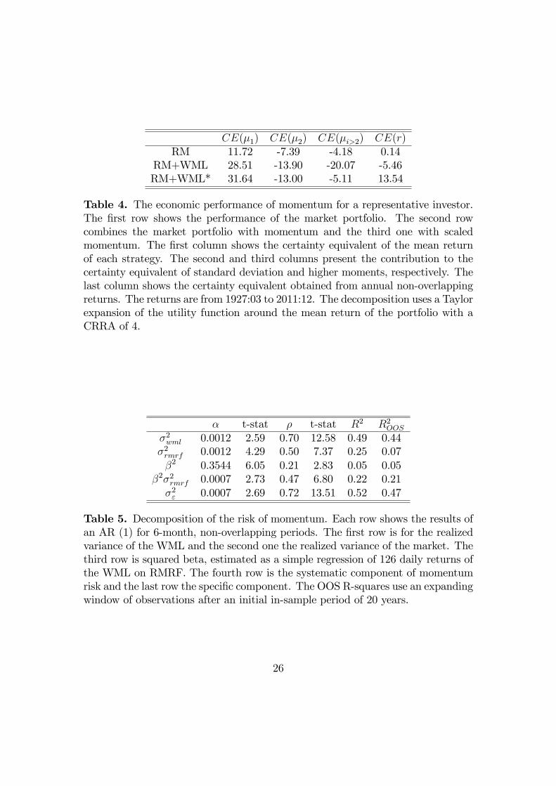
CE(�1) CE(�2) CE(�i>2) CE(r)RM 11.72 -7.39 -4.18 0.14

RM+WML 28.51 -13.90 -20.07 -5.46RM+WML* 31.64 -13.00 -5.11 13.54

Table 4. The economic performance of momentum for a representative investor.The �rst row shows the performance of the market portfolio. The second rowcombines the market portfolio with momentum and the third one with scaledmomentum. The �rst column shows the certainty equivalent of the mean returnof each strategy. The second and third columns present the contribution to thecertainty equivalent of standard deviation and higher moments, respectively. Thelast column shows the certainty equivalent obtained from annual non-overlappingreturns. The returns are from 1927:03 to 2011:12. The decomposition uses a Taylorexpansion of the utility function around the mean return of the portfolio with aCRRA of 4.

� t-stat � t-stat R2 R2OOS�2wml 0.0012 2.59 0.70 12.58 0.49 0.44�2rmrf 0.0012 4.29 0.50 7.37 0.25 0.07�2 0.3544 6.05 0.21 2.83 0.05 0.05

�2�2rmrf 0.0007 2.73 0.47 6.80 0.22 0.21�2" 0.0007 2.69 0.72 13.51 0.52 0.47

Table 5. Decomposition of the risk of momentum. Each row shows the results ofan AR (1) for 6-month, non-overlapping periods. The �rst row is for the realizedvariance of the WML and the second one the realized variance of the market. Thethird row is squared beta, estimated as a simple regression of 126 daily returns ofthe WML on RMRF. The fourth row is the systematic component of momentumrisk and the last row the speci�c component. The OOS R-squares use an expandingwindow of observations after an initial in-sample period of 20 years.

26

Country SR �SR CE �CEWML WML* WML WML*

FRANCE 0.67 1.03 0.36 2.50% 11.32% 8.82%GERMANY 1.02 1.39 0.38 11.32% 17.55% 6.23%JAPAN 0.08 0.24 0.15 -5.70% -3.01% 2.69%

UNITED KINGDOM 1.09 1.77 0.68 5.27% 27.76% 22.49%

Table 6. The Sharpe ratio and the certainty equivalent of plain momentum andscaled momentum (all measures are annualized). Original data from datastream.The returns for country-speci�c momentum portfolios are from Chaves (2012). Thescaled momentum uses the realized volatility in the previous 6-months, obtainedfrom daily data. The certainty equivalent uses annual overlapping returns andconsiders a CRRA of 4. The certainty equivalent assumes an investment in thedomestic risk-free rate asset of the US for all countries plus the respective long-short stock portfolio. The returns are from 1980:07 to 2011:10.

Periods CE*-CE CE*>CE (%) SR*-SR SR*>SR (%)1 year 3.09 62.96 0.06 60.383 years 7.95 76.30 0.15 79.155 years 10.66 85.61 0.17 83.4210 years 11.12 91.21 0.18 97.66

Table 7. Comparison of rolling-period Sharpe ratios and certainty equivalents ofraw momentum and risk-managed momentum (denoted with a star). We computethe monthly returns of both strategies for rolling, overlaping, intervals of one,three, �ve and ten years. From these, we obtain the certainty equivalent (assuminga CRRA of 4) and the Sharpe ratio for each interval. The �rst column reportsthe average di¤erence in certainty equivalent of the risk-managed strategy overraw momentum. The second column shows the percentage of intervals for whichthe risk-managed strategy outperformes the plain one. Columns 3 and 4 show thesame information for the Sharpe ratio. The returns are from 1927:03 to 2011:12.

27

Figures

30 35 40 45 50 55 60 65 70 75 80 85 90 95 00 05 10

100

101

102

103

104

105

Mom and FF factors: 1927:03­2011:12

cum

ulat

ive 

retu

rns 

(log 

scal

e) $2,135

$145

$475

$68,741

RMRFSMBHMLWML

Figure 1. The long-run cumulative returns of momentum compared to the Fama-French factors. Each strategy consists on investing $1 at the beginning of thesample in the risk-free rate and combine it with the respective long-short portfolio.The proceeds are fully reinvested till the end of the sample. On the right is theterminal value of each strategy.

28

30 31 32 33 34 35 36 37 38 390

0.5

1

1.5

2

2.5Mom and the market: 1930:01 to 1939:12

cum

ulat

ive 

retu

rns

$0.98

$0.1

00 01 02 03 04 05 06 07 08 090

0.5

1

1.5

2

2.5

3

3.5Mom and the market: 2000:01 to 2009:12

cum

ulat

ive 

retu

rns

$1.02$0.72

RMRF WML

Figure 2. Momentum crashes. The �gure plots the cumulative return and ter-minal value of the momentum and market portfolio strategies in its two mostturbulent periods: the 1930�s and the 2000�s.

29

30 35 40 45 50 55 60 65 70 75 80 85 90 95 00 05 10

20

40

60

80

100

120

The monthly realized volatility of momentum

annu

aliz

ed in

 p.p

.

Figure 3. The realized volatility of momentum obtained from daily returns ineach month from 1927:03 to 2011:12.

30

1 2 3 4 50

0.5

1

Risk and Risk

1 2 3 4 50

5

10

15

20

25Risk and Return

1 2 3 4 50

0.5

1

1.5

2Risk and SR

WML RMRF

Figure 4. The performance of the market factor ( �RMRF�) and momentum (�WML�) conditional on realized volatility in the previous 6 months. Returns aresorted into quintiles according with volatility in the previous 6 months for eachfactor. The �gure presents the following year volatility (computed from dailyreturns), the cumulative return in percentage points and the Sharpe Ratio. Thereturns are from 1927:03 to 2011:12.

31

30 35 40 45 50 55 60 65 70 75 80 85 90 95 00 05 10

100

101

102

103

104

105

106

Risk­managed momentum: 1927:03­2011:12

cum

ulat

ive 

log 

retu

rns

$68,741

$6,140,075

WMLWML*

Figure 5. The long-run performance of risk-managed momentum. The risk-managed momentum (WML*) scales the exposure to momentum using the realizedvariance in the previous 6-months. In the beginning of the sample the strategyinvests $1 in the risk-free asset and combines it with the long-short portfolio. Theproceeds are fully reinvested till the end of the sample. On the right is the terminalvalue of the strategy.

32

­80 ­60 ­40 ­20 0 20 400

2

4

6

8

10Density of WML and WML* monthly returns

­80 ­70 ­60 ­50 ­40 ­30 ­20 ­100

0.2

0.4

0.6

0.8

1Density of WML and WML* for returns lower than ­10 p.p.

WMLWML*

WMLWML*

Figure 6. The density of plain momentum (WML) and risk-managed momentum(WML*). The risk-managed momentum uses the realized variance in the previous6 months to scale the exposure to momentum. The returns are from 1927:03 to2011:12.

33

30 31 32 33 34 35 36 37 38 39

10­1

100

Risk­managed momentum: 1930:01 to 1939:12

cum

ulat

ive 

log 

retu

rns

$0.1

$1

00 01 02 03 04 05 06 07 08 09

100

Risk­managed momentum: 2000:01 to 2009:12

cum

ulat

ive 

log 

retu

rns

$0.72

$1.88

WML WML*

Figure 7. The bene�ts of risk-management in the 1930�s and the 00�s. The risk-managed momentum (WML*) uses the realized variance in the previous 6 monthsto scale the exposure to momentum.

34

30 35 40 45 50 55 60 65 70 75 80 85 90 95 00 05 10

0.2

0.4

0.6

0.8

1

1.2

1.4

1.6

1.8

2The weights of the strategy: 1927:03­2011:12

wei

ght o

n W

ML

Figure 8. Weights of the scaled momentum. The risk-managed momentum usesthe realized variance in the previous 6 months to scale the exposure to momentum.

35

50 55 60 65 70 75 80 85 90 95 00 05

101

102

103

104

105

106

107

Momentum and risk­managed momentum: 1945:01 to 2005:12

cum

ulat

ive 

retu

rns 

(log 

scal

e)

$147073

$862028

WMLWML*

Figure 9. Cumulative return of momentum and risk-managed momentum from1945:01 to 2005:12. The risk-managed momentum uses the realized volatility ofthe momentum strategy in the previous 6 months to scale the exposure and achievea target constant volatility of 12 percent (annualized).

36