Molecular simulation of the vapor-liquid equilibrium of methanethiol + propane mixtures

E L S E V I E R Fluid Phase Equilibria 131 (1997) 51-65

I

Molecular simulation of the vapor-liquid equilibrium of methanethiol + propane mixtures

Rupal Agrawal, Eric P. Wallis *

Phillips Petroleum Company, Research and Development, 331A Pl, PRC, Bartlescille, OK 74004, USA

Received 21 May 1996; accepted 17 November 1996

Abstract

We have used the Gibbs ensemble Monte Carlo (GEMC) method to calculate the vapor-liquid equilibrium properties for pure propane and methanethiol as well as their mixtures. We used two different potential-energy surfaces to describe the propane and methanethiol molecules. The results show that the simple site-site potential-energy surfaces work well for the pure components by optimizing the parameters to reproduce the liquid-phase density at the normal boiling point. For mixtures, the site-site potential-energy surface predicts the liquid-phase densities fairly well, but is not accurate enough to give quantitative results for the vapor-phase mole fraction for this system. © 1997 Elsevier Science B.V.

Keywords: Gibbs ensemble Monte Carlo simulations; Methanethiol; Propane; Mixture; Coexistence properties

1. I n t r o d u c t i o n

Molecular simulations use potential models which are fit to reproduce experimental data, usually for the pure components. Since the parameters are optimized only for the pure compounds, there is no guarantee that they will describe the interactions between dissimilar molecules in the mixtures correctly. Mixtures of polar and non-polar components, i.e. alcohols/alkanes, self-association of the polar species can occur which results in non-random mixing, and thus these systems can show large deviation from the ideal solution law [1]. Recent studies on strongly interacting systems [2-6], have shown that molecular simulations can predict mixture properties in good agreement with experiment. These studies employed simple potential models which were optimized to reproduce thermodynamic data for the pure components. However, they concentrated on the liquid phase and were performed mainly at ambient temperatures and pressures. Van Leeuwen and Smit [7] used simple two-body interactions to predict the coexistence curve for methanol by fitting the potential-energy parameters to

* Corresponding author.

0378-3812/97/$17.00 © 1997 Elsevier Science B.V. All rights reserved. PII S0378-3812(96)03225-6

52 R. Agrawal, E.P. Wallis/ Fluid Phase Equilibria 131 (1997) 51-65

reproduce the coexistence densities at two points along the saturation curve. Although this fitting method gives good results compared with experimental data, it assumes one knows some of the coexistence curve a priori. In this study, we test the ability of simple two-body interactions, that were fitted to reproduce the pure component liquid-phase density at the normal boiling point, to predict the vapor-liquid equilibrium for the mixture.

Using the Gibbs ensemble Monte Carlo (GEMC) computer simulation method, [8-11], the phase coexistence properties for pure components and mixtures can be calculated directly without specifying the chemical potential. The method has been used for simple systems [8-11] and complex fluids: both as pure components [7,12-17] and as mixtures [18-22].

Sulfur compounds, and their behavior with hydrocarbons, are important in the petroleum and chemical industry. The ability to accurately predict the vapor-liquid coexistence properties of mixtures is critical for the development of practical models which are used to design and optimize purification, separation and environmental processes. In particular, thiols (mercaptans) are an important class of compounds used as odorants in the storage of natural gas [23-27]. In earlier papers [28,29], we studied the thermodynamic properties of mercaptan in alkanes and showed that non-ideal behavior was present even at low concentrations of the mercaptan. In this study, we use potential-energy parameters which were optimized to reproduce the liquid density of pure propane and methanethiol at their normal boiling points and carry out GEMC simulations to calculate the vapor-liquid coexistence properties for propane( l )+ methanethiol(2) mixtures. We compare our results with experimental data as well as the COSTALD correlation [30-32] and the Redlich-Dunlop vapor density correlation [33].

2. Computational methods

2.1. Potential energy surface

The methanethiol (MESH) and propane molecules were modelled as rigid molecules in their equilibrium configurations [34,35] and the united atom representation was employed, that is, all CH 3 and CH 2 moieties were represented as single sites. Thus, MeSH consists of three sites, one centered on the CH 3 groups, one on the sulfur atom and one on the hydrogen atom. Propane is modelled with three sites, one on each CH n group.

Since the molecules are held rigid, the total potential-energy surface is given by summing all intermolecular interactions between each site i on molecule k and site j on molecule I according to

Ukl = °Lk~lqiqje2__ + It rij)[[°'ij]'2 (O'ij) 6]~/j 4Eij - - _ _

i j rij (1)

where rij is the distance between site i and site j and ~ij and o-ij are obtained using standard combining rules given by

eij = v/e, ej (2)

R. Agrawal, E.P. Wallis / Fluid Phase Equilibria 131 (1997)51-65 53

and

1 ,~ij = ~(,~, + ~j), (3)

where e i and o- i are the Lennard-Jones parameters for site i. Two potential-energy surfaces were employed in this study. The first potential-energy surface

(PES1) used the OPLS potential-energy parameters for liquid hydrocarbons [35] and thiols [34] unaltered. For simulations of pure components such as hydrocarbons and alcohols, OPLS parameters are generally adequate. However, the OPLS parameters do not perform as well for mixtures of polar and non-polar mixtures. For example, interactions between highly polar species and weakly polar hydrocarbons are completely ignored since hydrocarbons are uncharged in the OPLS parameteriza- tion. Therefore, partial atomic charges were obtained from ab initio calculations. The charge parameters, q, for all of the atomic sites on each molecule for PES2 were obtained from ab inito calculations at the Hartree Fock level using the 6-31G * basis set [36] holding the molecule rigid in its gas-phase configuration. The partial charges for all the atomic sites were determined via fits to the electrostatic potentials obtained from the calculated wavefunction using the CHELPG routine in Gaussian 92 [37]. Then, for each CH n group, the partial charges on the hydrogen atoms were summed to the carbon atoms to give the charge for the CH n group. This resulted in reducing the number of sites per molecule, which made the run-times much shorter. Since the partial charges had been modified, we had to adjust the • and tr parameters to reproduce the pure component liquid-phase density at the normal boiling point. This set of adjusted parameters will be referred to as PES2. To calculate the density for the liquid phase, we use the isothermal-isobaric ensemble (NPT) method implemented in CChAPPs [38]. The calculated density for the pure components using our modified model (PES2) are in good agreement with literature values (see below).

Component Temperature (°C) Exp

O (g c c - t )

PES1 PES2

MeSH 5.96 0.888 a 0.867 + .006 0.888 + .007

Propane -42 .07 0.581 b 0.551 + .003 0.583 + .002

a Ref [391. b Ref [40].

The potential-energy parameters for both PES1 and PES2 are listed in Table 1. The factor e 2 in Eq. (1) is 332.18 kcal A tool -1.

Intermolecular interactions were truncated according to a spherical cut-off based on the center-of- mass distance between molecules. The cut-off value was a little less than half the box length. Corrections to the potential energy arising from truncations of intermolecular interactions were calculated according to [41]

M M on M k on M / zc

Ec,, = 27rNE E E E f x, ptr~go(r)uij(r)dr, (4) k t i j r~

where M is the number of different components in the solution, x k = Nk/N, Pt = NI/V, where N is

54 R. Agrawal, E.P. Wallis / Fluid Phase Equilibria 131 (1997) 51-65

Table 1

Site parameters for methanethiol and propane ~

Site PES 1 PES2

orb e c q d orb ~c q d

CH 3 (MESH) 3.775 0.207 0.18 3.775 0.280 0.161

S 3.550 0.250 - 0.45 3.550 0.338 - 0.361 H 0.000 0.000 0.27 0.000 0.000 0.200

CH 3 (propane) 3.905 0.175 0.00 3.870 0.190 - 0.100 CH 2 (propane) 3.905 0.118 0.00 3.870 0.128 0.200

The geometries for both MeSH and propane are held fixed at rcs = 1.82 A,

a c c c = I 12.0 °. b Units are angstroms. c Units are kcal m o l - t

d Units are electrons.

rsH = 1.34 ,~, rcc = 1.53 ,~, acs n = 96.0 ° and

the total number of molecules (N = N~ + N 2 + ... + N m), V is the volume of the cube, rij is the radial distance between sites i and j, gij is the radial distribution function between sites i and j (assumed to be unity beyond the cutoff distance re), and uij is the intermolecular pairwise interaction between sites i and j. A correction was not made for the truncated electrostatic interaction, since the effects have been shown to be small for water [2,34,42,43] and methyl iodide [17].

2.2. Gibbs ensemble Monte Carlo procedure

The Gibbs ensemble Monte Carlo (GEMC) calculations were carried out using standard proce- dures, including periodic boundary conditions, Metropolis sampling [44] and the Gibbs ensemble [8-11], using the computer program CChAPPs [38]. One drawback of the standard GEMC method is the slow convergence of the vapor-phase due to the low acceptance of insertions. Recent advances have helped increase the sampling efficiency of the Gibbs ensemble method [45-48]. The total number of molecules for each run was between 200-250, depending on the simulation conditions. The initial densities at a new temperature or pressure were taken as the final densities from the previous temperature or pressure simulation. New configurations were generated by randomly selecting a molecule, translating it randomly in all three Cartesian directions, and randomly rotating it about a randomly chosen axis. After every 500 configurations, one volume change and 50-300 molecular transfers were attempted. The ranges for the molecular and volume moves were chosen to yield an acceptance ratio of about 0.45 for new configurations. The acceptance ratio for the molecular transfers depended on the number of attempts and the density of the liquid phase. The average acceptance ratio ranged from 0.01% for conditions far from the critical point to 9.0% near the critical.

To test for convergence of the simulation, we monitored the average chemical potential for each component in each phase. The chemical potential is estimated during the particle transfer step using the Widom "test particle" method which was formulated for the Gibbs ensemble [49] and written here for region 1:

kTln{ V! e -t~avl+) (5) ll'i = - - \ N I . i + 1 '

R. Agrawal, E.P. Wallis / Fluid Phase Equilibria 131 (1997) 51-65 55

where AU ÷ is the configurational energy change of region I during attempted transfers of particles of species i.

The initial configuration of each phase was generated by a randomly distributing the molecules on a cubic lattice and randomly orienting them. The volume of the cube was determined by the initial density and number of molecules. Each simulation was melted for 0.5 × 106 steps which consisted of only molecular translations and rotations and then equilibrated for 1.0 × 10 6 steps which were discarded. Averages of the computed properties were obtained over an additional 3.0 × 10 6 configurations for the pure component simulations and 3.0-5.0 × 10 6 configurations for the mixtures. The statistical uncertainties ( + lo-) reported were obtained from averages over 5 subsets of each simulation. For a system of 216 molecules, a sequence of 1 × 10 6 steps took approximately 5 h of CPU time on an IBM RISC/6000 model 590 workstation.

In order to estimate the critical properties, the vapor and liquid densities were fitted to the law of rectilinear diameters

- - = Pc + C , ( T - T~) (6) Pl + Pv

and the law of order parameter scaling

Pl - P~ - C2( L - T) ~ -

2 (7)

where /3 c is the critical exponent taken as 0.313 for the 3-D Ising model [50] (see Appendix A for a detailed derivation and example calculation).

3. Results and discussion

Gibbs ensemble Monte Carlo (GEMC) simulations were performed using two different potential- energy surfaces to describe propane and methanethiol. The standard OPLS potential-energy parameters were used for PES 1 while for PES2, the q, e and o- were adjusted to better reproduce the liquid density at normal boiling point conditions (see Section 2.1).

The average properties were calculated using configurations which were saved every 500 steps during the MC run. Unfortunately, we know of no experimental vapor-liquid coexistence density data for pure methanethiol or the propane(1)/methanethiol(2) mixture. Therefore, the densities of methanethiol, propane and the mixture were taken from correlation equations. The correlations should predict the density of propane well enough for this study. The liquid-phase densities were estimated using the COSTALD [30-32] correlation while the vapor-phase densities were estimated using the Redlich-Dunlop vapor density correlation [33]. The experimental data for the P -xy diagram for the propane(1)/methanethiol(2) mixture were taken from the work by Eng and Wilson [51].

3.1. Vapor-liquid equilibrium for propane

GEMC simulations were performed for different temperatures from the normal boiling point of T = 231 to 365 K. For PES 1, only four simulations were performed over this range of temperatures while for PES2, six simulations were performed. Fig. 1 shows the convergence of the liquid and vapor


e~

B1 0.7

0.6

0.5

0.4 - ~ ................... :=:=z==:-_=:==::: A1

0.3

0.2

0.1 B2 ~_'_'_'_'_---_-_--_-_'_'__~_._ ___ __~ ..................................... 0 ............................................................................. A2 .....................

a h t L t 1000 2000 3000 4000 5000 6000

# of Steps/500

Fig. 1. Convergence of the liquid and vapor densities for pure propane at T = 340 K and pure methanethiol at T = 393 K. The solid lines represent the cumulative averages and the standard deviations are the dashed lines: A1 is liquid-phase propane, A2 vapor-phase propane, B 1 is liquid-phase methanethiol, B2 is vapor-phase methanethiol.

-5.2

-5.4

-5.6

I i . Wr t/J"~! -5.8 i

-6 I~ " Y J ....... [~" - ~ : ; ~ " ............... ~'~ .....................

-6.2 [ ' . . . . 0 1000 2000 3000 4000 5000 6000

# of Steps/500

Fig. 2. Convergence of the liquid and vapor phase chemical potential for pure propane at T = 340 K and pure methanethiol at T = 393 K: - - propane, - - - methanethiol.

Table 2 Coexistence densities for pure propane

T (K) PES1 PES2 Correlation

pn (gcc -n) pv(gCc -1) p n ( g c c - I ) p v ( g c c - j ) p n ( g c c - n ) b p v ( g c c - n ) c

231 0.551 +0.008 0.0084+0.0002 0.582+0.002 0.0050+0.0003 0.5816 0.0025 273 0.538 ± 0.003 0.0071 ± 0.0007 0.5269 0.0103 300 0.459 ± 0.005 0.023 + 0.001 0.4890 0.0220 313 0.486±0.006 0.0170___0.0009 0.4656 0.0310 340 0.387 ± 0.009 0.059 ± 0.004 0.434 ± 0.006 0.0337 ± 0.0003 0.4069 0.0611 355 0.22+0.09 0.091 _+0.009 0.40_+0.06 0.2±0.03 365 0.33 ± 0.02 0.30 ± 0.07 0.2460 0.1760

a The final temperature was above the critical temperature for this potential-energy surface (see the text). b Values were obtained using the COSTALD correlation [30-32]. c Values were obtained using the Redlich-Dunlop correlation [33].

400

350

Correlation • PF~I

m 300 [ -

250

200

R. Agrawal, E.P, Wallis / Fluid Phase Equilibria 131 (1997) 51-65 57

I I I I I

0 0.1 0.2 0.3 0.4 0.5 0.6

p (g/co)

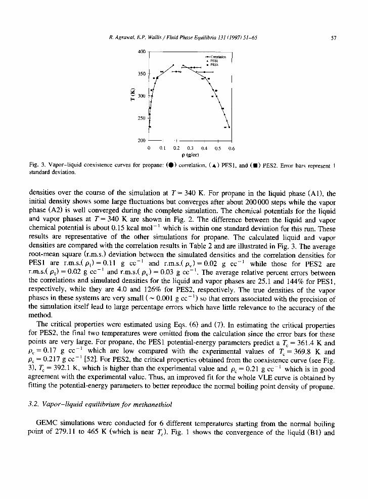
Fig. 3. Vapor-liquid coexistence curves for propane: (O) correlation, ( , ) PES1, and (11) PES2. Error bars represent 1 standard deviation.

densities over the course of the simulation at T = 340 K. For propane in the liquid phase (A1), the initial density shows some large fluctuations but converges after about 200 000 steps while the vapor phase (A2) is well converged during the complete simulation. The chemical potentials for the liquid and vapor phases at T = 340 K are shown in Fig. 2. The difference between the liquid and vapor chemical potential is about 0.15 kcal mol - 1 which is within one standard deviation for this run. These results are representative of the other simulations for propane. The calculated liquid and vapor densities are compared with the correlation results in Table 2 and are illustrated in Fig. 3. The average root-mean square (r.m.s.) deviation between the simulated densities and the correlation densities for PES1 are r .m . s . (p l )=0 .11 g cc -~ and r .m . s . (pv )=0 .02 g cc -~ while those for PES2 are r.m.s.(Pl) = 0.02 g cc -~ and r.m.s.(Pv) = 0.03 g cc -1. The average relative percent errors between the correlations and simulated densities for the liquid and vapor phases are 25.1 and 144% for PES1, respectively, while they are 4.0 and 126% for PES2, respectively. The true densities of the vapor phases in these systems are very small ( ~ 0.001 g cc-1) so that errors associated with the precision of the simulation itself lead to large percentage errors which have little relevance to the accuracy of the method.

The critical properties were estimated using Eqs. (6) and (7). In estimating the critical properties for PES2, the final two temperatures were omitted from the calculation since the error bars for these points are very large. For propane, the PES1 potential-energy parameters predict a Tc = 361.4 K and p c = 0 . 1 7 g cc -~ which are low compared with the experimental values of Tc=369.8 K and Pc = 0.217 g cc-~ [52]. For PES2, the critical properties obtained from the coexistence curve (see Fig. 3), T c = 392.1 K, which is higher than the experimental value and Pc = 0.21 g cc - t which is in good agreement with the experimental value. Thus, an improved fit for the whole VLE curve is obtained by fitting the potential-energy parameters to better reproduce the normal boiling point density of propane.

3.2. Vapor-liquid equilibrium for methanethiol

GEMC simulations were conducted for 6 different temperatures starting from the normal boiling point of 279.11 to 465 K (which is near To). Fig. 1 shows the convergence of the liquid (B1) and


Table 3 Coexistence densities for pure methanethiol

PES 1 PES2 Correlation

T(K) P l (gcc - I ) Pv(gCc-I) P l (gcc - I ) Pv(gcc - t ) p~(gcc- I )b Pv(gcc I)c

279 0.854 + 0.009 0.009 + 0.002 0.888 + 0.005 0.007 + 0.0007 0.8612 0.0022 313 0.795+0.005 0.0271 +0.0005 0.836+0.002 0.0096+0.001 0.8160 0.0072 355 0.69 + 0.01 0.054 + 0.007 0.768 + 0.009 0.022 + 0.001 0.7530 0.0187 393 0.51 +0.03 0.11 +0.02 0.6851 +0.005 0.0603+0.01 0.6859 0.0411 431 0.29_+0.05 0.29-t-0.05 0.59_+0.02 0.186-+0.003 0.5977 0.0856 465 0.43 _+ 0.06 0.22 + 0.05 0.3563 0.2320

a The final temperature was above the critical temperature for this potential-energy surface (see the text). b Values were obtained using the COSTALD correlation [30-32]. c Values were obtained using the Redlicb-Dunlop correlation [33].

vapor (B2) densities for pure methanethiol over the course of the simulation at T = 393 K. Both the liquid and vapor phases for pure methanethiol are well equil ibrated during the course of the

simulation. The average chemical potentials for the liquid and vapor phases at T = 393 K are illustrated in Fig. 2. For this simulation, the difference in chemical potential between the liquid and

vapor phase is less than 0.1 kcal m o l - l , which is less than the simulation uncertainty. To test the

effects o f longer simulations on the calculated results for the density, we extended the run at T = 393 K f rom 3.0 × 10 6 to 19.0 × 10 6 steps and saw no appreciable differences in the l iquid-phase or

vapor-phase densities. The liquid and vapor densities for both the correlation and the simulation results are given in Table 3 and illustrated in Fig. 4. The average r.m.s, deviation between the experimental densities and our simulated results using PES1 are r . m . s . ( p l ) = 0 . 1 6 g cc - l and

r .m.s . (Pv) = 0.10 g cc - l while those for PES2 are r .m.s . (P l ) - 0.01 g cc - l and r .m.s . (Pv) = 0.04 g cc-~ . The average relative percent errors between the correlations and simulated densities for the liquid and vapor phases are 26.2 and 249% for PES1, respectively, while they are 2.2 and 144% for

PES2, respectively.

500 Correlation

400450 = ~ • 1'~2

[,. 350

300

250 I I I I

0 0.2 0.4 0.6 0.8 p (g/cc)

Fig. 4. Vapor-liquid coexistence curves for methanethiol: (O) correlation, ( • ) PES 1 and ( • ) PES2. Error bars represent 1 standard deviation.


0.7

0.6

0.5

0.4

~ 0.3

0.2

0.1

, , , , , f , , ,

, . . . ~ . q ' ~ k a i ~

• . ~ . ,

, . . . . . . , . . , , , ,

i i i i i i " i i i

100 200 300 400 500 600 700 800 900 1000 # of Steps/2000

Fig. 5. Convergence of the liquid and vapor densities for p ropane ( l )+ methanethiol(2) mixture at T = 313 K and 10.0 atm. The solid lines represent the cumulative averages, the small dash lines represent the instantaneous densities, and the standard deviations are the long dashed lines.

For pure methanethiol, the PES1 parameters predicted a T c = 418 K and Pc = 0.30 g cc-~ which are low compared with the experimental values [52] of 469.8 K and 0.3315 g cc -~, respectively. Using PES2, the resulting coexistence curve (see Fig. 4) gives a good prediction of the critical properties, Tc = 457 K and Pc = 0.34 g cc-~. Therefore, by fitting the potential-energy parameters to better reproduce the normal boiling point liquid density for methanethiol, we obtained a better overall representation of the VLE curve.

3.3. VLE f o r p r o p a n e ( l ) + MESH(2) mix ture

For the propane( l )+ methanethiol(2) mixture, five GEMC simulations were conducted at a temperature of 313.15 K and pressures of 5.5, 7.0, 8.5, 10.0, 11.5 atm. The simulations were performed using both the PES1 or PES2 parameters unaltered from the pure component calculations

-3

-3.5

o -4 .5

' ~-22_.~ --:-_ __: _222r22 --_-.= -6

-6.5

-7 0 100 200 300 400 500 600 700 800 900 1000

# of Steps/2000

Fig. 6. Convergence of the liquid and vapor chemical potentials for p ropane ( I )+ methanethiol(2) mixture at T = 313 K and 10.0 atm.: - - propane, - - - methanethiol.


0.8

0.7

0.6

0.5

......................................................... y£t) ...............

. . . . . . . . . . . . . . . . . . . . . . . . . . . . . . . . . . . . . .

x(1)

0 4 . , i , i , , , i ,

0 1 0 0 2 0 0 3 0 0 4 0 0 5 0 0 6 0 0 7 0 0 8 0 0 9 0 0 1 0 0 0 # of Steps/2000

Fig. 7. Convergence of the liquid (x) and vapor (y) mole fractions for propane(l) + methanethiol(2) mixture at T = 313 K and 10.0 atm. Mole fractions x(l) and y(l) are of propane. The solid lines represent the cumulative averages and the standard deviations are the dashed lines.

and combining the potential-energy parameters for dissimilar sites according to Eqs. (2) and (3). Fig. 5 illustrates the convergence of the average density for the liquid and vapor phases of the propane(1)/methanethiol(2) mixture at T = 313 K and P = 10.0 atm. The dashed lines represent l o- deviation. As the figure shows, the density is well equilibrated over the length of the simulation. The average chemical potentials for propane and methanethiol, at T = 313 K and P = 10.0 atm, are illustrated in Fig. 6. The difference in the liquid and vapor chemical potential for both species (see Fig. 6) is within the standard deviation of the simulation which is about + 0.8 kcal m o l - ~ for propane and ___ 0.6 kcal mol-~ for methanethiol. Fig. 7 illustrates the convergence of the mole fraction for propane. The mole fraction takes longer to equilibrate as is shown in Fig. 7. The liquid mole fraction of propane, x(1), is fairly well equilibrated after 600000 steps. The propane vapor mole fraction, y(1), has much larger fluctuations and therefore, takes longer to equilibrate but is within the error bars within 600000 steps. The small number of molecules in the vapor phase makes this phase more sensitive to the addition or subtraction of particles compared with the liquid phase.

We compared the pressure-composit ion ( P - x y ) data obtained from the five simulations to the experimental results of Eng and Wilson. [51] The P - x y curves for the experimental data and those predicted using PES 1 and PES2 are given in Table 4 and shown in Fig. 8. For the liquid phase, both PES1 and PES2 predict the composition in very good agreement with the experimental data. The

Table 4 P -xy data for the propane(l)+ methanethiol(2) mixture a

P (atm) PES 1 PES2 Experiment

x(l) y(l) x(1) y(1) x(l) y(1)

5.5 11.6+0.2 40+2 9.9+0.1 47+3 9.08 44.43 7 13+1 47+5 16+1 34+10 16.17 56.32 8.5 25+ 1 61 +5 28+ 1 55___5 28.50 66.67 10 45+ 1 68+3 47.9+0.2 72+2 47.32 75.39 11.5 70+1 77+1 71.6+0.5 76+5 70.20 84.0

a x and y represent the mole percent of propane in the liquid and gas phase, respectively.


14

- - Ealmim~t x ( 1 ) ~ ~ • PK.~I

12 ,, I , ~2

- . ._- : ~ 6

4 ~

2 I I i i 20 40 60 80 100

x(1),y(1) Fig. 8. P - x y diagram for propane(l)+methanethiol(2) mixture at 313 K. Mole percents x(1) and y( l ) are of propane: ( - - ) experiment, ( • ) PES 1 and ( • ) PES2. Error bars represent 1 standard deviation.

average r.m.s, deviations between the simulations and experimental results for the liquid phase using PES1 and PES2 are r.m.s.(x(1)) = 0.02 and 0.007, respectively. For the vapor phase, the comparison is not as good with the average r.m.s, deviations for PES1 and PES2 being r.m.s.(y(1)) = 0.06 and 0.09, respectively. The average relative percent errors for the mole fractions in the liquid and vapor phases are 13.6 and 9.3% for PES1, respectively, while those for PES2 are 4.0 and 16.4%, respectively. A possible explanation for the poor agreement in the vapor-phase composition is that the potential models used were developed to match the liquid phase properties and therefore incorporate some three-body as well as polarization effects, which are important in the liquid phase in the two-body interactions, and these effects are probably not present in the vapor phase of the real system. This effect was observed in VLE calculations of pure water [53,54] as well as in alkane mixtures [55].

The liquid and vapor densities for the simulation results using PES 1 and PES2 are given in Table 5 and illustrated in Fig. 9. Unfortunately, we know of no experimental data with which to compare our coexistence density results, but we can compare the predicted liquid-phase densities with those

Table 5 Coexistence densities for propane (1)+ methanethiol(2) mixtures ~

P (atm) PES1 PES2 COSTALD b

P l ( g c c - I ) P v ( g c c - I ) P l ( g c c - l ) P v ( g c c i) P l ( g c c i)

3.2 0.795+_0.005 0.0271 ___0.0005 0.836_+0.002 0.009+0.001 0.8160 5.5 0.733 ___ 0.004 0.0202 + 0.0006 0.78 _+ 0.02 0.034 _+ 0.004 0.7773 7 0.725 ± 0.009 0.029 +_ 0.007 0.760 _+ 0.007 0.012 +_ 0.003 0.7484 8.5 0.662___0.007 0.029_+0.003 0.712_+0.005 0.017+0.006 0.7003

10 0.57 _+ 0.01 0.037 + 0.005 0.639 +- 0.006 0.029 +- 0.002 0.6323 11.5 0.499+_0.008 0.05 _+0.01 0.560+-0.003 0.017 +_0.003 0.5568 13.42 0.459 ± 0.005 0.023 ___ 0.001 0.486 _+ 0.006 0.0170 _+ 0.0009 0.4678

a The temperature is T = 313 K. b Values were obtained using the COSTALD correlation [30-32].

6 2 R. Agrawal, E.P. Wallis / Fluid Phase Equilibria 131 (1997) 51-65

14

12 ¸

1 0

6

4 -

2

0

CO~TALD • • PESI

i

?

-

mA •

I P I f

0.2 0.4 0.6 0.8

p (g/cc)

Fig. 9. Vapor-liquid coexistence curves for propane(l) + methanethiol(2): (O) correlation, ( • ) PES 1 and ( • ) PES2. Error bars represent 1 standard deviation.

predicted by the COSTALD correlation, since earlier work showed that this correlation gives accurate predictions of the mixture densities for the n-butanethiol + n-heptane system [29]. The average relative errors between the correlation and simulation results for the liquid-phase densities are 6.3 and 2.0% for PES1 and PES2, respectively. For the liquid phase, PES1 does a fairly good job in predicting the mixing behavior, but by fitting the potential-parameters to better reproduce the thermodynamic data for the pure components at their normal boiling points (PES2), we get better agreement for this phase over a large range of pressures and compositions. We do not compare the vapor-phase densities since we are unsure of the accuracy of the correlations for this phase.

4. Conclusions

Our results show that simple site-site potential-energy models, optimized for the pure components, can adequately describe the pure component coexistence behavior, but do not yield quantitative results for mixture properties of this systems. In this study, two potential-energy surfaces were used, PES 1 and PES2. For PES 1, the OPLS potential-energy parameters for propane and methanethiol were used unaltered, while for PES2, the potential-energy parameters were adjusted to better reproduce the liquid-phase densities at the normal boiling conditions for the pure components. For the mixtures, the potential-energy surfaces were used unaltered from the pure components simulations and standard mixing rules were employed to calculate the interactions between dissimilar sites. Monte Carlo simulations in the Gibbs ensemble (GEMC) have been performed for pure propane and methanethiol at temperatures ranging for the normal boiling point to near the critical points and for propane(1)/methanethiol(2) mixtures at 313 K and pressures of 5.5, 7.0, 8.5, 10.0 and 11.5 atm in order to calculate the vapor-liquid equilibrium properties for these mixtures. The coexistence curves for the pure components are in very good agreement with the correlation data. For propane, the relative error between the experimental and predicted critical temperatures, T c, is 2.2% for PES 1 and 6.2% PES2, while the relative error for the critical density, Pc, is 21.6% for PES1 and 3.2% for PES2. For methanethiol, the relative error between the experimental and predicted T c is 11.1% for PES I and

R. AgrawaL E.P. Wallis / Fluid Phase Equilibria 131 (1997) 51-65 63

2.8% for PES2, while that for Pc is 9.5 and 2.6% for PES1 and PES2, respectively. For mixtures of propane(i) + methanethiol(2), the average r.m.s, deviation between the simulations and experimental mole fractions of propane in the liquid phase using PES1 and PES2 are r.m.s.(x(1)) = 0.02 and 0.007, respectively, while the comparison for the vapor phase is not as good with the average r.m.s. deviations for PES1 and PES2 being r.m.s.(y(1)) = 0.06 and 0.09, respectively. The average relative percent errors for the mole fractions in the liquid and vapor phases are 13.6 and 9.3% for PES1, respectively, while those for PES2 are 4.0 and 16.4%, respectively. The average relative errors for the liquid-phase densities are 6.3 and 2.0% for PES 1 and PES2, respectively. One possible suggestion for the poor agreement in the vapor-phase composition is that the potential models were developed to match the liquid-phase densities for the pure components and therefore have some three-body effects as well as polarization effects, which are important in the liquid phase, incorporated into the two-body interactions. These two-body interactions are then used to describe the molecules in both the liquid and vapor phase. Since the composition of a near-ideal vapor phase is a measure of the interactions in the liquid phase, potential models which more accurately describe the molecular interactions should increase the accuracy of the models. The results are encouraging in that good qualitative predictions of the complete coexistence curves can be obtained using these simple site-site potential-energy models with limited experimental data.

Acknowledgements

The authors would like to thank George Parks, Don Lauffer, R.W. Hankinson and Bill Parrish for helpful comments and suggestions about this research. EPW would also like to thank A.Z. Pana- giotopoulos (Cornell University) for helpful discussions during this work.

References

[1] J.S. Rowlinson and F.L. Swinton, Liquids and Liquid Mixtures, 3rd ed., Butterworths, 1982. [2] X.-W. Wu, Y.-G. Li, J.-F. Lu, T. Teng, Monte carlo simulation of the water-methanol system, Fluid Phase Equil., 77

(1992) 139-156. [3] P.F.W. Stouten and J. Kroon, Computation confirms contraction: A molecular dynamics study of liquid methanol,

water and a methanol-water mixture, Mol. Simulations, 5 (1990) 175. [4] C.A. Koh, H. Tanaka, J.M. Walsh, K.E. Gubbins, J.A. Zollweg, Thermodynamic and structural properties of

methanol-water mixtures: experiment, theory, and molecular simulations, Fluid Phase Equil., 83 (1993) 51-58. [5] Y. Adachi and K. Nakanishi, Monte carlo study of self-association of methanol in benzene, Mol. Simulations, 6 (1991)

299. [6] Y. Adachi and K. Nakanishi, Monte carlo study of local structure in benzene-methanol mixtures, Fluid Phase Equil.,

83 (1993) 69. [7] M.E. Vanleeuwen and B. Smit, Molecular simulation of the vapor-liquid coexistence curve of methanol, J. Phys.

Chem., 99 (1995) 1831. [8] A.Z. Panagiotopoulos, Direct determination of phase-coexistence properties of fluids by Monte Carlo simulation in a

new ensemble, Mol. Phys., 61 (1987) 813. [9] A.Z. Panagiotopoulos, N. Quirke, M. Stapleton, D.J. Tildesley, Phase equilibria by simulation in the Gibbs ensemble:

Alternative derivation, gerneralization and application to mixture and membrane equilibria, Mol. Phys., 63 (1988) 527-545.


[10] A.Z. Panagiotopouios, Direct determination of fluid phase equilibria by simulation in the Gibbs ensemble: A review, Mol. Simulations, 9 (1992) 1.

[11] A.Z. Panagiotopoulos, Gibbs Ensemble Techniques, in NATO ASI Ser. C. 1995, Kluwer Academic Publishers. [12] R.F. Cracknell, D. Nicholson, N.G. Parsonage, H. Evans, Rotational insertion bias: A novel method for simulating

dense phases of structured particles, with particular application to water, Mol. Phys., 71 (1990) 931-943. [13] M. Laso, J.J. dePablo and U.W. Suter, Simulation of phase equilibria for chain molecules, J. Chem. Phys., 97 (1992)

2817. [14] J.I. Siepmann, S. Karaborni and B. Smit, Vapor-liquid equilibria of model alkanes, J. Am. Chem. Soc., 115 (1993)

6454. [15] J.I. Siepmann, S. Karaborni and B. Smit, Simulating the critical properties of complex fluids, Nature, 365 (1993) 330. [16] K. Esselink, P.A.J. Hilbers, S. Karaborni, J.I. Siepmann, B. Smit, Simulating complex fluids, Mol. Simulation, 14

(1995) 259-274. [17] F.F.M. Freitas, F.M.S.S. Fernandes and B.J.C. Cabral, Vapor-liquid equilibrium and structure of methyl iodide liquid,

J. Phys. Chem., 99 (1995) 5180. [I 8] J.J, dePablo and J.M. Prausnitz, Phase Equilibria for Fluid Mixtures From Monte Carlo Simulation, Fluid Phase Equil.,

53 (1989) 177. [19] J.J. dePablo, J.M. Prausnitz, H.J. Strauch, P.T. Cummings, Molecular simulation of water along the liquid-vapor

coexistence curve from 25 °C to the critical point, J. Chem. Phys., 93 (1990) 7355. [20] J.J, dePablo, M. Bonnin and J.M. Prausnitz, Vapor-liquid equilibria for polyatomic fluids from site-site computer

simulations: pure hydrocarbons and binary mixtures containing methane, Fluid Phase Equil., 73 (1992) 187. [21] H.J. Strauch and P.T. Cummings, Computer simulation of vapor-liquid equilibrium in mixed solvent electrolyte

solutions, Fluid Phase Equil., 83 (1993) 213. [22] H.J. Strauch and P.T. Cummings, Gibbs Ensemble Simulation of Mixed Solvent Electrolyte Solutions, Fluid Phase

Equil., 86 (1993) 147. [23] M.L. Whisman, J.W. Goetzinger, F.O. Cotton, D.W. Brinkman, C.J. Thompson, A New Look at Odorization Levels for

Propane Gas, Technical Information Center, US Dept. of Energy, 1977. [24] R.W. Hankinson and G.M. Wilson, Vapor-Liquid Equilibrium Data for Ethyl Mercaptan in Propane Vapors., Proc.

Annu. Conv. Nat. Gas Process. Assoc., 53 (1974) 98. [25] D. Zudkevitch and G.M. Wilson, Phase Equilibria in Solutions of Methyl Mercaptan and Light Hydrocarbons., Proc.

Annu. Conv. Nat. Gas Process. Assoc., 53 (1974) 101. [26] J.W. Goetzinger, D.W. Brinkman, B.E. Poling, M.L. Whisman, Vapor-liquid equilibrium data of ethanethiol and

tetrahydrothiophene in propane., J. Chem. Eng. Data, 22 (1977) 396. [27] H. Ng and D.B. Robinson, Vapor-liquid equilibrium in propane-odorant systems, Gas Processors Assoc., RR-113,

January 1989. [28] E.P. Wallis, Monte carlo study of the thermodynamics and structural properties of thiol-propane mixtures, Fluid Phase

Equil., 103 (1994) 97. [29] E.P. Wallis, Monte Carlo study of the thermodynamic and structural properties of 1-butanethiol + N-heptane mixtures,

Mol. Simulation, 14 (1995) 177. [30] R.W. Hankinson and G.H. Thomson, A new correlation for saturated densities of liquids and their mixtures, Am. Inst.

Chem. Eng. J., 25 (1979) 653. [31] G.H. Thomson, K.R. Brobst and R.W. Hankinson, An improved correlation for densities of compressed liquids and

liquid mixtures, J. Am. Inst. Chem. Eng., 28 (1982) 671. [32] R.C. Reid, J.M. Prausnitz and B.E. Poling, The Properties of Gases and Liquids, 4th ed., McGraw-Hill Book Company,

1987. [33] R.C. Reid and T.K. Sherwood, The Properties of Gases and Liquids, 1st ed., McGraw-Hill Book Company Inc., 1958. [34] W.L. Jorgensen, Intermolecular potential functions and monte carlo simulations for liquid sulfur compounds, J. Phys.

Chem., 90 (1986) 6379. [35] W.L. Jorgensen, J.D. Madura and C.J. Swenson, Optimized intermolecular potential functions for liquid hydrocarbons,

J. Am. Chem. Soc., 106 (1984) 6638. [36] H.A. Carlson, T.B. Nguyen, M. Orozco, W.L. Jorgensen, Accuracy of free energies of hydration for organic molecules

from 6-31 G-asterisk-derived partial charges, J. Computat. Chem., 14 (1993) 1240-1249. [37] M.J. Frisch, G.W. Trucks, M. Head-Gordon, P.M.W. Gill, M.W. Wong, J.B. Foresman, B.G. Johnson, H.B. Schlegel,


M.A. Robb, E.S. Replogle, R. Gomperts, J.L. Andres, K. Raghavachari, J.S. Binkley, C. Gonzalez, R.L. Martin, D.J. Fox, D.J. Defrees, J. Baker, J.J.P. Stewart, J.A. Pople, GAUSSIAN-92, Gaussian Inc., Pittsburgh, 1992.

[38] E.P. Wallis, Computational Chemistry at Phillips Petroleum (CChAPPs), Phillips Petroleum Company, Bartlesville, Oklahoma, 1995.

[39] API, Selected values of physical and thermodynamic properties of hydrocarbons and related compounds, American Petroleum Institute Research Project 44, Carnegie Press, 1953.

[40] A. Berthound and R.J. Brum, Thermodynamics of methanethiol, J. Chim. Phys. Phys.-Chim. Biol., 21 (1924) 143. [41] M.P. Allen and D.L. Tildesley, Computer Simulations of Liquids, Oxford University Press, 1987. [42] W.L. Jorgensen and J.D. Madura, Solvation and conformation of methanol in water, J. Am. Chem. Soc., 105 (1983)

1407. [43] W.L. Jorgensen and J.D. Madura, Temperature and size dependence for Monte Carlo simulations of TIP4P water, Mol.

Phys., 56 (1985) 1381. [44] N. Metropolis, A.W. Rosenbluth, M.N. Rosenbluth, A.H. Teller, E. Teller, Equation of state calculations by fast

computing machines, J. Chem. Phys., 21 (1953) 1087. [45] J.P. Valleau, Density-scaling Monte-Carlo study of subcritical Lennard-Jonesium, J. Chem. Phys., 99 (1993) 4718. [46] N.B. Wilding, Critical-point and coexistence-curve properties of the Lennard-Jones fluid: A finite-size scaling study,

Phys. Rev. E, 52 (1995) 602. [47] F.A. Escobedo and J.J. Depablo, A new method for generating volume changes in isobaric-isothermal Monte Carlo

simulations of flexible molecules, Macromolecular Theory and Simulations, 4 (1995) 691. [48] G. Orkoulas and A.Z. Panagiotopoulos, Phase diagram of the two-dimensional Coulomb gas: A thermodynamic scaling

Monte Carlo study, J. Chem. Phys., 104 (1996) 7205. [49] B. Smit and D. Frenkel, Calculation of chemical potential in the Gibbs ensemble, Mol. Phys., 68 (1989) 951. [50] D. Chandler, Introduction to Statistical Mechanics, Oxford University Press, 1987. [51] W.W.Y. Eng, Vapor-Liquid Equilibrium Behavior of Thiol Binary Systems Studied by the Total Pressure Method

Thiol Group Contribution Model, in Department of Chemical Engineering, 1977, Brigham Young University, Salt Lake, p. 61.

[52] R.P. Danner and T.E. Daubert (eds.), Tables of Physical and Thermodynamic Properties of Pure Compounds, AIChE Design Institute for Physical Property Research, Vol. Project 801, 1993, The Pennsylvania State University, University Park, Pennsylvania.

[53] H.J. Strauch and P.T. Cummings, Comment on: Molecular simulation of water along the liquid-vapor coexistence curve from 25°C to the critical point, J. Chem. Phys., 96 (1992) 864.

[54] J.J. de Pablo, J.M. Prausnitz, H.J. Strauch, P.T. Cummings, Molecular simulation of water along the liquid-vapor coexistence curve from 25°C to the critical point, J. Chem. Phys., 93 (1991) 7355.

[55] J.J. de Pablo, M. Bonnin and J.M. Prausnitz, Vapor-liquid equilibria for polyatomic fluids form site-site computer simulations: pure hydrocarbons and binary mixtures containing methane, Fluid Phase Equil., 73 (1992) 187.

Molecular simulation of the vapor-liquid equilibrium of methanethiol + propane mixtures

Documents

Transcript of Molecular simulation of the vapor-liquid equilibrium of methanethiol + propane mixtures