EJECTION FORCES AND STATIC FRICTION COEFFICIENTS

FOR RAPID TOOLED INJECTION MOLD INSERTS

DISSERTATION

Presented in Partial Fulfillment of the Requirements for

the Degree Doctor of Philosophy in the Graduate School of

The Ohio State University

By

Mary E. Kinsella, M.S.

* * * * *

The Ohio State University 2004

Dissertation Committee: Approved by

Professor Blaine Lilly, Adviser

Professor Jose Castro ______________________________

Professor Jerald Brevick Adviser Industrial and Systems Engineering Graduate Program

ii

ABSTRACT

While manufacturing is typically considered a high-volume industry, the necessity

for small quantities of products and components exists for aerospace customers and those

producers wishing to mass customize their products. Because of the high cost of tooling,

injection molding processes are seldom used to produce only small quantities of parts.

This, however, can be remedied if cost effective tooling methods are implemented.

Rapid prototyping processes show great potential for such tooling applications because

they generally require shorter lead times, produce less waste, and, in some cases, use less

expensive materials.

The research presented herein studies the feasibility of using injection mold

inserts produced with additive methods by investigating ejection and friction. Through

experimentation, the application of P-20 steel, laser sintered LaserForm ST-100, and

stereolithography SL 5170 tools to produce limited quantities of a thin-walled cylindrical

part are explored. A substantial amount of data and statistical analysis are provided that

reveal conditions during the actual injection molding process, and comparisons are made

among the three insert types. Experimental ejection forces from each tool type are

compared with model-based calculations, and apparent coefficients of static friction are

calculated and compared to standard test results. Based on the data and analyses, the

benefits and limitations of using rapid tooled injection mold inserts are presented.

iii

For Michael, Amelia, and Nathaniel

iv

ACKNOWLEDGMENTS

“Gratitude is not only the greatest of virtues, but the parent of all the others.”

--Cicero

At the Materials and Manufacturing Directorate in the Air Force Research

Laboratory, I am grateful to Charlie Browning, Bill Russell, and Chuck Wagner for

providing the time and funding to complete this research; to John Jones for assembling

and programming the data acquisition system; and to Neal Ontko, Nick Jacobs, and Ben

Gardner for performing friction tests.

At the NASA Marshall Space Flight Center, thanks to Ken cooper, who provided

the laser sintered and stereolithography inserts for the experimental work.

At The Ohio State University, many thanks to the following people: Brian

Carpenter for finite element modeling of the inserts for thermal and deformation

simulations, and for helping with experiments; Bob Miller for his machining and

injection molding expertise; Mary Hartzler for providing machining services and design

consultation; Barney Barnhart for providing equipment and expertise for the

thermoplastic tensile tests; Mauricio Cabrera-Rios for design of experiments and

statistical analysis consultation; Narayan Bhagavatula for helping with tensile tests and

injection molding simulations; and especially my adviser, Dr. Blaine Lilly, and Drs. Jose

Castro and Jerry Brevick for serving on my dissertation committee.

Finally, I extend my gratitude to my parents, Robert and Carolyn Corbin, who

deserve more than I can ever express.

v

VITA

June 5, 1961 Born – Longview, WA, USA 1983 Bachelor of Science, Applied Science Miami University, Oxford, OH, USA 1983 - 1986 Production Supervisor, NCR Microelectronics Fort Collins, CO, USA 1987 - Present Project Engineer, Materials and Manufacturing Directorate US Air Force Research Laboratory Wright-Patterson AFB, OH, USA 1991 Master of Science, Materials Engineering University of Dayton, Dayton, OH, USA

PUBLICATIONS

Kinsella, M. E., Heberling, M. E. 1997, “Applying Commercial Processes to Defense Acquisition,” National Contract Management Journal, vol. 28, issue 1, p. 11. Kinsella, M. E., Lilly, B. L., Bhagavatula, N., Cooper, K. G. 2002, “Application of Solid Freeform Fabrication Processes for Injection Molding Low Production Quantities: Process Parameters and Ejection Force Requirements for SLS Inserts,” Proceedings of the 13th Annual Solid Freeform Fabrication Symposium, Austin, TX, pp. 92-100.

FIELDS OF STUDY

Major Field: Industrial and Systems Engineering

vi

TABLE OF CONTENTS

Abstract ........................................................................................................... ii

Acknowledgments.......................................................................................... iv

Vita .................................................................................................................. v

Table of Contents ........................................................................................... vi

List of Figures ................................................................................................ xi

List of Tables................................................................................................. xv

Chapter 1 Introduction .................................................................................... 1

1.1 Background ........................................................................................................... 1

1.2 Problem Statement ................................................................................................ 6

1.3 Research Objective.............................................................................................. 10

1.4 Research Description........................................................................................... 11

1.5 Organization........................................................................................................ 12

Chapter 2 Literature Search .......................................................................... 14

2.1 Ejection Force ..................................................................................................... 14

2.1.1. Ejection Force Models............................................................................... 14

2.1.2 Shrinkage ................................................................................................... 22

vii

2.1.3 Friction and Adhesion ................................................................................ 25

2.2 Rapid Tooling ..................................................................................................... 34

2.2.1 Background ................................................................................................ 34

2.2.2 Stereolithography and Laser Sintering for Injection Molding Tools........... 44

2.2.3 Summary .................................................................................................... 48

Chapter 3 Theory........................................................................................... 50

3.1 Thermoplastic Materials...................................................................................... 50

3.1.1 High Impact Polystyrene ............................................................................ 51

3.1.2 High Density Polyethylene ......................................................................... 54

3.2 The Adhesion Component of Friction ................................................................. 55

3.3 Ejection Force Model Derivation ........................................................................ 60

3.3.1 Model derivation ........................................................................................ 60

3.3.2 Additional Consideration for Strain............................................................ 65

Chapter 4 Experimentation ........................................................................... 66

4.1 Friction Testing ................................................................................................... 66

4.1.1 Friction Test Apparatus .............................................................................. 68

4.1.2 Test Matrix and Procedure ......................................................................... 70

4.2 Measurement of Elastic Modulus ........................................................................ 72

4.3 Injection Molding................................................................................................ 75

4.3.1 Mold Design and Materials ........................................................................ 75

4.3.2 The Injection Molding Process ................................................................... 79

4.3.3 Design of Experiments ............................................................................... 84

viii

4.3.4 Experimental Procedure ............................................................................. 87

4.4 Set-up and Data Acquisition................................................................................ 88

4.4.1 Temperature Measurement and Thermal Model ......................................... 89

4.4.2 Ejection Force Measurement ...................................................................... 98

4.4.3 Diameter and Thickness Measurement ..................................................... 100

4.4.4 Calculation of Static Friction Coefficient ................................................. 101

Chapter 5 Results and Analysis .................................................................. 102

5.1 Injection Molding Experiments ......................................................................... 103

5.1.1 Experimental Results and Discussion....................................................... 103

5.1.2 HDPE Experimental Ejection Force Results............................................. 105

5.1.3 HIPS Experimental Ejection Force Results .............................................. 107

5.1.4 Experimental Ejection Force Results from the P-20 and ST-100 Inserts .. 109

5.1.5 Experimental Ejection Force Results from the SL 5170 and SL 5170/P-20

Inserts................................................................................................................ 109

5.2 Statistical Analysis ............................................................................................ 112

5.2.1 DOE Results............................................................................................. 112

5.2.2 Main Effects and Interactions................................................................... 112

5.3 Standard Friction Testing Results...................................................................... 120

5.3.1 HDPE Standard Friction Results .............................................................. 120

5.3.2 HIPS Standard Friction Results ................................................................ 124

5.4 Reliability of the Data ....................................................................................... 128

5.5 Calculation of Ejection Force Using the Model................................................. 130

ix

5.5.1 Calculated Ejection Force for HDPE........................................................ 133

5.5.2 Calculated Ejection Force for HIPS.......................................................... 134

5.5.3 Possible Sources of Error ......................................................................... 135

5.6 Calculation of Apparent Friction Coefficients using the Menges Model ........... 138

5.6.1 HDPE Apparent Coefficient of Friction Results....................................... 140

5.6.2 HIPS Apparent Coefficient of Friction Results......................................... 141

5.6.3 Apparent Friction Coefficient Results from the P-20 and ST-100 Inserts. 143

5.6.4 Apparent Friction Coefficient Results from the SL 5170 and SL 5170/P-20

Inserts................................................................................................................ 144

5.6.5 Comparing Calculated Friction Results to Standard Friction Test Results 146

5.7 Other Observations of Rapid Tooled Inserts...................................................... 150

Chapter 6 Conclusions ................................................................................ 156

6.1 Molding HDPE and HIPS with ST-100 and SL 5170 Inserts ............................ 156

6.1.1 Benefits and Limitations of Using Rapid Tooled Injection Mold Inserts .. 156

6.1.2 Friction and Ejection Force Considerations.............................................. 158

6.2 Using a Model to Determine Ejection Force and the Coefficient of Friction..... 160

6.3 Implications and Future Work........................................................................... 162

6.4 Summary........................................................................................................... 165

LIST OF REFERENCES ............................................................................ 167

Appendix A Data Tables............................................................................. 174

A.1 Tensile Test Data Table.............................................................................. 176

A.2 Modulus Look-up Table ............................................................................. 177

x

A.3 Thermal Analysis Convergence Table ........................................................ 178

A.4 Sample Experimental Data Set, All Runs ................................................... 182

A.5 Sample Experimental Part Dimensions (2 Runs Shown) ............................ 184

A.6 Experimental Data and Calculated Coefficient of Friction (Menges), Run

Average............................................................................................................. 185

A.7 Analysis of Variance Tables by Set ............................................................ 187

Appendix B Mold and Canister Drawings.................................................. 190

B.1 Part Drawing............................................................................................... 191

B.2 Mold Insert Drawings ................................................................................. 192

B.3 Mold Assembly Drawings .......................................................................... 205

xi

LIST OF FIGURES

Figure 1.1: Importance characteristics for various tool types……………………….. .4

Figure 2.1: A schematic of the laser engineered net shaping (LENS™) process…... 36

Figure 2.2: A schematic of the selective laser sintering process……………………. 38

Figure 2.3: A schematic of the stereolithography process…………………………...42

Figure 3.1: Polystyrene monomer……………………………………………………52

Figure 3.2: High impact polystyrene………...…………………………… ............... 53

Figure 3.3: Polyethylene monomer. .......................................................................... 55

Figure 3.4: High density polyethylene linear molecule. ............................................ 55

Figure 3.5: Thin-walled cylindrical pressure vessel. ................................................. 61

Figure 3.6: Section of the part and the core with associated stresses. ........................ 62

Figure 4.1: Schematic of friction apparatus............................................................... 68

Figure 4.2: Friction test apparatus: sled on plate specimen inside furnace and tester…

.................................................................................................................................. 69

Figure 4.3: Tensile testing apparatus with tube furnace............................................ 73

Figure 4.4: HIPS specimens after tensile tests.......................................................... 74

Figure 4.5: Elastic modulus at various temperatures for HDPE and HIPS. .............. 74

Figure 4.6: Sprue side of the MUD base mounted in the injection molding machine

with SL 5170 cavity insert. ....................................................................................... 76

xii

Figure 4.7: Core and cavity inserts, before final machining, made of SL 5170, P-20

steel, and LaserForm ST-100. ................................................................................... 76

Figure 4.8: Canister part with vent holes and no taper.............................................. 78

Figure 4.9: Sumitomo SH50M injection molding machine. ..................................... 79

Figure 4.10: Signal conditioner and computer with front panel for data acquisition,

and core side of mold with thermocouple and load cell sensor wires. ....................... 89

Figure 4.11: Thermocouple placement within core insert.......................................... 90

Figure 4.12: Representative thermal traces of the injection molding cycle............... 91

Figure 4.13: Graphs of the thermal analysis results for each material combination... 94

Figure 4.14: Representative ejection force traces ...................................................... 99

Figure 4.15: Digital pictures of HDPE canisters for measuring inside and outside

diameter. ................................................................................................................. 101

Figure 5.1: Experimental ejection force results for HDPE, all runs. ....................... 106

Figure 5.2: Experimental ejection force values for HIPS, all runs.......................... 108

Figure 5.3: Experimental ejection force results from the P-20 and ST-100 inserts. 110

Figure 5.4: Experimental ejection force results from the SL 5170 insert and the

combination SL 5170/P-20 insert. ........................................................................... 111

Figure 5.5: Main effects and interactions for HDPE with the P-20 insert............... 114

Figure 5.6: Main effects and interactions for HIPS with the P-20 insert................. 115

Figure 5.7: Main effects and interactions for HDPE with the ST-100 insert. ......... 116

Figure 5.8: Main effects and interactions for HIPS with the ST-100 insert. ........... 117

Figure 5.9: Main effects and interactions for HDPE with the SL 5170/P-20 insert.118

xiii

Figure 5.10: Main effects and interactions for HIPS with the SL 5170/P-20 insert.119

Figure 5.11: Standard friction test results for HDPE; means and ranges shown in the

table. ....................................................................................................................... 122

Figure 5.12: Standard friction test results for HIPS; means and ranges shown in the

table. ....................................................................................................................... 123

Figure 5.13: Sample plot of load vs. time for HIPS on SL 5170 from elevated

temperature tests. .................................................................................................... 126

Figure 5.14: Sample plot of load vs. time for HIPS on P-20 from elevated

temperature tests. .................................................................................................... 127

Figure 5.15: Calculated values for ejection force for HPDE compared with

experimental values, averaged across all runs. ........................................................ 134

Figure 5.16: Calculated values for ejection force for HIPS parts from the P-20 and

ST-100 cores compared with experimental values, averaged across all runs........... 137

Figure 5.17: Calculated values for ejection force for HIPS parts from the SL 5170

core compared with experimental values, averaged across all runs. ........................ 137

Figure 5.18: Calculated values of the apparent coefficient of static friction for HDPE,

all runs. ................................................................................................................... 140

Figure 5.19: Apparent coefficients of friction calculated from experimental results

for HIPS, P-20 and ST-100 results only, and results from all runs. ......................... 142

Figure 5.20: Apparent coefficient of static friction for parts from the P-20 insert. . 143

Figure 5.21: Apparent coefficient of static friction for parts from the ST-100 insert.

................................................................................................................................ 144

xiv

Figure 5.22: Apparent coefficient of static friction for parts from the SL 5170 insert.

................................................................................................................................ 145

Figure 5.23: Apparent coefficient of static friction for parts from the SL 5170 core

with the P-20 cavity. ............................................................................................... 146

Figure 5.24: Average apparent coefficient of static friction for HDPE compared to

standard test results. ................................................................................................ 148

Figure 5.25: Average apparent coefficient of static friction for HIPS compared to

standard test results. ................................................................................................ 149

Figure 5.26: Defects in the SL 5170 core. .............................................................. 152

Figure 5.27: Simulation results of HDPE injection into SL 5170 insert, no packing.

................................................................................................................................ 153

Figure 5.28: Simulation results of HIPS injection into SL 5170 insert, no packing.154

Figure 5.29: Simulation results of HIPS injection into SL 5170 insert, with packing.

................................................................................................................................ 155

Figure A.1: Sample plots from tensile test data. ...................................................... 175

xv

LIST OF TABLES

Table 1.1: Properties of tooling materials.................................................................... 9

Table 2.1: Vanguard System Specifications from 3D Systems.................................. 40

Table 2.2: LaserForm ST-100 (Sintered and Infiltrated) Material Properties from 3D

Systems. .................................................................................................................... 40

Table 2.3: SLA 250 System Specifications from 3D Systems. .................................. 43

Table 2.4: Vantico SL5170 Typical Properties (90-minute UV post cure). ............... 43

Table 4.1: Friction data for polymers on steel. .......................................................... 67

Table 4.2: Friction test matrix. ................................................................................. 71

Table 4.3: Injection molding machine specifications................................................ 80

Table 4.4: Injection Molding Parameters .................................................................. 82

Table 4.5: Typical data for Lutene-H ME9180. ........................................................ 83

Table 4.6: Typical data for BASF PS 495F. .............................................................. 83

Table 4.7: Experimental design for six sets, including process parameters. ............. 86

Table 4.8: Resulting convergence times from the thermal simulation. ..................... 93

Table 4.9: Input conditions for the thermal analysis. ................................................. 93

Table 5.1: Experimental ejection force results for HDPE and HIPS according to

packing time, cooling time, and packing pressure parameters. ................................ 104

xvi

Table 5.2: Results from the designed experiment indicating which factors had a

significant effect on ejection force. ......................................................................... 113

Table 5.3: Surface roughnesses of all plates (friction tests) and cores (injection

molding experiments).............................................................................................. 129

Table 5.4: Calculated values of ejection force for HDPE from the Menges equation

and experimental data. ............................................................................................ 131

Table 5.5: Calculated values of ejection force for HIPS from the Menges equation

and experimental data. ............................................................................................ 132

Table 5.6: Calculated apparent coefficient of friction results according to packing

time, cooling time, and packing pressure parameters. ............................................. 139

1

CHAPTER 1

INTRODUCTION

1.1 Background

Manufacturing is predominantly a high volume industry and is constantly striving

toward greater efficiencies at lower cost. A growing sector of manufacturers, both in the

aerospace and consumer markets, however, is targeting small quantity production to meet

customer needs. The demand for low volume production is strong in the aerospace

industry, where customer organizations such as the military services and NASA need

relatively small numbers of end products to accomplish their missions. Product variety is

generally higher, and lot sizes smaller, in the defense industry compared to other

industries. The U.S. Defense Department and other government organizations have been

focused on finding ways to build low volume products more cost effectively (e.g.,

Kinsella 2000). These organizations and their contractors must implement new methods

of producing extremely robust equipment in reduced time at reduced cost (Kaminsky

1996).

2

Small production quantities in the consumer market have historically applied to

prototypes and market testing. In the past decade, however, market forces have altered

the way industry looks at low volume requirements. Increasing product variety and

shorter product lifetimes have led to mass customization, in which products are designed

and made to order for individual customers, but produced by methods that still allow for

economies of scale. Mass customization is already evident in a number of industries,

including pagers, fiber optics, and blue jeans (Victor & Boynton 1998). The concept

continues to spread as customers become more particular and manufacturers become

more flexible.

Thermoplastic injection molding is inherently well suited to high volume

production requirements. A quality mold, running with material and process variables

under tightly controlled conditions, is capable of producing very large quantities of parts

with little or no manual intervention. When coupled with automated material feeding and

robotic part removal systems, injection molding operations can be extremely cost

effective over large production runs, turning out millions of components per year at a cost

of a few pennies per part. At these production scales, the cost of the tooling essentially

disappears, and the part cost results almost entirely from material, handling, and

overhead.

Minimum economic production quantities for injection molded parts are typically

large due to tooling costs, which are incurred at the beginning of the product life. Molds

are expensive, regardless of part size, and typically require production volumes of tens of

thousands of parts in order to amortize their costs. For this reason, injection molding is

3

generally feasible only when the total production run is large enough to recoup the cost of

the tool. Many design situations exist in which the complexity and versatility of injection

molded thermoplastics would be an ideal solution were it not for the high initial cost of

the tooling. For many low volume applications, the ability to use the best engineering

solution is inhibited by the inability to cost effectively produce the necessary tooling.

Injection molds expressly designed for low volumes have successfully been

fabricated for prototyping use and as bridge tools. Small numbers of prototypes are

typically built to test out a design for fit and function, and to allow changes to be made

before tooling designs are finalized. Since so many consumer products use injection

moldings, it is often necessary to build prototype tools to produce the design prototypes,

especially in cases where the prototype must be fully functional to answer questions of

strength, rigidity, etc. Bridge molds, on the other hand, are built and put into production

very quickly. That is, they produce a small volume of parts prior to the completion of

the final tooling, thus “bridging” the gap between prototype tools and final production.

While prototype tooling can reduce time to market by accelerating the product

development cycle, bridge tooling is designed to get a new product to market quickly

while the high volume production tooling is still under construction. In both cases,

reduced time to market is the prime consideration, and the cost of the tooling will

eventually be folded into the total tooling cost and amortized over the lifetime of the

product.

As opposed to prototype and bridge tooling, molds intended specifically for low

volume production have many fewer products over which to amortize costs. In low

4

volume production environments, tooling must be low cost, unless the product is very

expensive. Time to market is a secondary consideration in this scenario. For these

reasons, the strategies for determining tooling methods will differ between prototype or

bridge tooling and low volume production tooling.

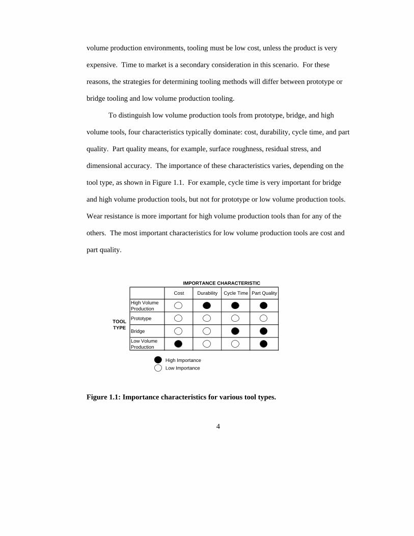
To distinguish low volume production tools from prototype, bridge, and high

volume tools, four characteristics typically dominate: cost, durability, cycle time, and part

quality. Part quality means, for example, surface roughness, residual stress, and

dimensional accuracy. The importance of these characteristics varies, depending on the

tool type, as shown in Figure 1.1. For example, cycle time is very important for bridge

and high volume production tools, but not for prototype or low volume production tools.

Wear resistance is more important for high volume production tools than for any of the

others. The most important characteristics for low volume production tools are cost and

part quality.

Figure 1.1: Importance characteristics for various tool types.

High Volume Production

Prototype

Bridge

Low Volume Production

High Importance

Low Importance

TOOL TYPE

IMPORTANCE CHARACTERISTIC

Cost Durability Cycle Time Part Quality

5

There are a few ideas that have been implemented for reducing tooling costs for

low volume production. For example, a less expensive tooling material can be used that

is easier to machine, such as aluminum instead of steel. Universal mold bases with

interchangeable inserts are another possibility, though this can be problematic if the piece

parts differ widely in design. “Family molds,” in which several components of an

assembly are molded together in the same tool, have been used with limited success due

to constraints imposed by filling and cooling. Any or all of these approaches can be

implemented to minimize tooling costs.

The application of rapid prototyping processes for the purpose of making tools,

known as rapid tooling, has been the object of much interest for prototype and low

volume production. Rapid tooling encompasses many processes based on the rapid

prototyping concepts of additive, layer-by-layer manufacturing. While these processes

are still finding their way into the injection mold market, they hold significant potential

for tools intended to build small quantities of parts.

Depending on the process used, rapid tooled molds are made from various

materials, which typically have much lower strength and thermal conductivity than the

tool steel used in conventionally machined molds. For these reasons, it is generally

believed that rapid tooled molds are inadequate for quality production injection molding.

If, however, the mold is required only to make a small quantity of products, and if

molding conditions are allowed to vary from those used with machined steel molds, rapid

tooling may be an economical alternative. These variations may occur at the expense of

6

cycle time, but cycle time is generally not considered to be as critical for low volume

production.

1.2 Problem Statement

Manufacturers who currently build products in small quantities, such as aerospace

systems, can benefit from injection molding tools that will cost effectively produce low

volumes of production parts. A growing need for such tools is evidenced by the

increasing applications for mass customization. Furthermore, if injection molds for low

volume production become economically feasible, then manufacturers will most likely

discover their overwhelming potential.

Aerospace applications that require small quantities of molded parts, especially

for the military, include composites and electronics packaging. In the composites area,

injection molding and related processes can be used to mold filled thermoplastics for

structural components or for resin transfer, such as for aircraft skins. Future aerospace

applications will also include micro molding for microelecromechanical systems.

Mass customization refers to the mass production of customized products

(Anderson & Pine 1997). The goal of mass customization is to develop, produce, market,

and deliver affordable goods and services with enough variety and customization that

nearly everyone finds exactly what they want (Pine 1993, p. 44). A modular approach to

injection molding using rapid tooled inserts facilitates mass customization at the

fabrication level, allowing smaller quantities to be customized economically.

7

Thermoplastic injection molds, in general, must perform several functions,

including distribution of the melt, formation of the melt into its final shape, cooling of the

melt, and ejection of the part. To meet these requirements, high volume molds are

traditionally machined of steel, are very strong, and have good thermal properties. Rapid

tooling processes, on the other hand, may be very well suited to building injection molds

for small quantity production. These processes have certain advantages for tooling

applications. For example, because rapid tooling processes can generate complex

geometries as easily as simple ones, they can build mold shapes and cooling lines that are

impossible to machine. Also, the capability for local composition control further

enhances the appeal of rapid tooled injection molds.

The material properties of rapid tools, however, vary from conventional molds,

i.e., strength and thermal conductivity can be much lower than for machined steel (Table

1.1). But for small quantity production, the robust material properties exhibited by

conventional machined steel molds may not be necessary. With less rigorous molding

parameters, such as injection pressures and temperatures, rapid tools might be used

successfully for injection molding. The properties of rapid tools may be adequate to meet

many small quantity injection molded part requirements, such as those for the aerospace

and mass customization industries. This research studied aspects of rapid injection mold

tooling in an attempt to find out if this is true.

The issue addressed in this research was whether or not rapid tooled injection

mold inserts are suitable for small quantity injection molding. Many aspects must be

researched in order to confirm any suitability, too many to address in a single project.

8

Therefore, this work has focused on aspects related to ejection force. Rapid tooling

materials must be able to withstand the forces inherent in the injection molding process,

including forces resulting from ejection of the molded part. Ejection force requirements

and the effects of process parameters on ejection force were investigated in this work.

Also included was the determination and analysis of friction coefficients from standard

test results, injection molding experiments, and an ejection force model. With respect to

these areas, this research provides a comparison of rapid tooled inserts to conventional

steel inserts, and further provides an assessment of the benefits and limitations of rapid

tooled inserts for injection molding small quantities of parts.

9

Table 1.1: Properties of tooling materials.

Process Mold Material Density Tensile Strength Hardness Conductivitykg/m3 MPa W/moC

BaselineMachining P-20 Mold Steel [1] 7870 1080 30-35 HRC 47.6 @ 204oC

H-13 Tool Steel [1] 7800 1550 52 HRC 25.1 @ 199oC

Moldmax XL (R) [2] 8900 760 28-32 HRC 63-70

(copper-nickel-tin)

Rapid Tooling Materials [2]3D Printing - Prometal Bronze/infiltrant 8100 406 60 HRB 7.35

Laser Sintering - 3D Systems Copper polyamide 3450 33.6 75 ShoreD 1.28 @ 40oC0.92 @ 150oC

S Steel w/bronze 7700 510 79 HRB 49 @ 100oCas machined 56 @ 200oC

Laser Generating - LENS S Steel 316 8000 [3] 800 80 HRB [3] 15 [3]

Plastic Casting -CIBA Ceramic-filled Epoxy 64 (UFS) 91 ShoreD

Stereolithography - 3D Systems SL 5170 cured resin 1220 59 85 ShoreD 0.200

[1] ed. Rubin 1990[2] From company literature[3] From www.matweb.com, various ss 316 properties

10

1.3 Research Objective

The purpose of this research was to determine the feasibility of using rapid tooled

inserts for injection molding small quantities of products. The objective was to

quantitatively determine the benefits and limitations of laser sintered and

stereolithography tools by: 1) comparing ejection force requirements among materials, 2)

learning which process parameters affect them, and 3) determining the friction

coefficients between the injection mold insert core and the thermoplastic part. The data

generated help to answer the following questions for two thermoplastic molding materials

(one amorphous and one crystalline) and two types of rapid tooled mold inserts:

• How do ejection forces compare among conventional and rapid tooled

injection mold inserts?

• How do model-based values for ejection force compare to experimentally

measured values?

• Do cooling time, packing pressure and packing time affect ejection forces for

conventional and rapid tooled injection mold inserts in a similar manner?

• What are the coefficients of friction between the thermoplastic materials and

the core materials during ejection?

• How do standard friction coefficient test results compare to model-based

calculations?

• Based on these data, what are the potential benefits and limitations for using

rapid tooled inserts for small quantity injection molding?

11

1.4 Research Description

The present research investigated the ejection portion of the thermoplastic

injection molding process. First, ejection forces were measured experimentally for parts

produced from steel, laser sintered steel (infiltrated with bronze), and stereolithography

resin mold inserts. A full factorial statistical experiment was designed to determine the

effects of three process parameters on the ejection force. Second, the experimental

ejection force values were compared to calculated values from an ejection force model.

Standard friction testing was conducted to determine static friction coefficients to use in

the model. Model-based values for the static friction coefficients were also determined

and compared with the standard test results. These results, along with observations of

tool performance, provide some indication of how successfully the rapid tooled inserts

might apply to injection molding.

The chosen part for the experiments is a vented, closed-end cylinder, similar to

the plastic canisters used to store photographic film. The thermoplastic materials were

chosen according to their moldability for the given application and their range of

applications for manufacturing and consumer products. High density polyethylene

(HDPE), a semicrystalline thermoplastic, and high impact polystyrene (HIPS), an

amorphous thermoplastic, are widely used consumer resins, and are known to be well

suited to injection molding.

The experimental core and cavity pairs were built as inserts that were fitted to a

standard mold base. The rapid tooling processes and materials have been chosen

12

according to their potential application for injection molding and to their availability for

experimentation. These processes are laser sintering and stereolithography. While the

experiments with the laser sintered insert were similar to those with the baseline steel

insert, the stereolithography insert posed more of a challenge due to the softness of the

material and its insulating qualities.

The number of experimental runs was determined by the designed experiment,

which varied three input parameters: packing pressure, packing time, and cooling time.

These input parameters are key in defining an optimal injection molding process and

producing a quality part. For each experimental part, ejection force, temperature at

ejection, and part diameter data were collected. The ejection force data were compared

with values calculated using a model for estimating ejection force developed by Menges.

Apparent coefficients of friction for all material pairs were calculated using the Menges

model and data from the experiments. These values were compared with results from

standard friction tests. Statistical analysis was performed to determine the effects of the

three input parameters on ejection force.

1.5 Organization

The remainder of this document is organized as follows. Chapter 2 is the result of

a literature search of relevant previous work. It first presents topics related to ejection

forces in injection molding, such as ejection force models, shrinkage, friction and

13

adhesion. A section on rapid tooling is also presented that includes a background of rapid

prototyping processes and details of the stereolithography and laser sintering processes.

Chapter 3 presents the theoretical basis for this work. This includes the materials

aspects of the two thermoplastics used in the experiments, HDPE and HIPS, and further

definition of the coefficient of friction. The last section in Chapter 3 derives the equation

for ejection force.

Chapter 4 provides details on how the experimental work was accomplished. It

describes the standard friction test, the injection molding experimental design, the part

and tool designs and data acquisition. Chapter 5 presents all test and experimental results

and statistical analysis, and Chapter 6 presents conclusions, implications and future work.

References are listed following Chapter 6. There are two appendixes: Appendix A

includes data tables, and Appendix B includes part and tool drawings.

14

CHAPTER 2

LITERATURE SEARCH

This chapter presents comprehensive results of a literature search on the topics of

ejection force and rapid tooling. Extensive work has been published on topics related to

ejection forces, including shrinkage, friction, adhesion, and modeling. Topics cited in

rapid tooling include various rapid prototyping processes and works specifically

pertaining to stereolithography and laser sintering.

2.1 Ejection Force

2.1.1. Ejection Force Models

Several researchers have developed force equations for the ejection of parts from

injection mold cores based on mechanical or thermo-mechanical models. Most of these

equations derive from the friction-based concept ApfF AR ××= (see derivation in

Chapter 3), where FR is the ejection (or release) force, f is the coefficient of friction

between the mold and the part, pA is the contact pressure of the part against the mold

15

core, and A is the area of contact. While area is a straightforward measure, friction

coefficient and contact pressure have various interpretations or methods of estimation. A

number of models and variations are summarized below.

The version of the ejection force equation developed by Menges et al for a vented

cylinder defines contact pressure as

mrA sdTEp ×∆×= )( 2.1

and therefore ejection force is:

LsdTEfF mrR π2)( ××∆××= 2.2

where E(T) is the elastic modulus of the thermoplastic part material at ejection

temperature, ∆dr is the relative change in diameter of the part immediately after ejection,

sm is the thickness of the part, and L is the length of the part in contact with the mold core

(Menges, Michaeli, & Mohren 2001). The rationale for this formulation is that shrinkage

of the part is constrained by the core, thus causing stresses to build up in the cross

sections of the part and resulting in forces normal to the surfaces restrained from

shrinking. When the part is ejected from the mold, the stored energy-elastic forces can

recover spontaneously. The relative change in circumference, measured immediately

after ejection, is used as a measure of tensile strain in the cross section of the part while it

is still on the core. The strain multiplied by the elastic modulus, the surface area in

16

contact, and an assumed friction coefficient then gives an estimate of the force required

to remove the part from the core.

Malloy and Majeski (1989) referenced the ejection force equation as used by

Menges et al and a more detailed version by Glanvill, as shown below. Their paper

examined ejection variables with respect to designing ejector pins.

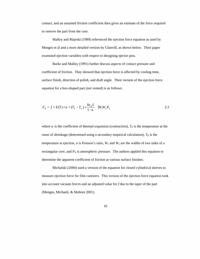
Burke and Malloy (1991) further discuss aspects of contact pressure and

coefficient of friction. They showed that ejection force is affected by cooling time,

surface finish, direction of polish, and draft angle. Their version of the ejection force

equation for a box-shaped part (not vented) is as follows:

( )Am

ESR PWWLs

TTTEfF 2118

)()( +−

×−×××=ν

α 2.3

where α is the coefficient of thermal expansion (contraction), TS is the temperature at the

onset of shrinkage (determined using a secondary empirical calculation), TE is the

temperature at ejection, ν is Poisson’s ratio, W1 and W2 are the widths of two sides of a

rectangular core, and PA is atmospheric pressure. The authors applied this equation to

determine the apparent coefficient of friction at various surface finishes.

Michalski (2000) used a version of the equation for closed cylindrical sleeves to

measure ejection force for film canisters. This version of the ejection force equation took

into account vacuum forces and an adjusted value for f due to the taper of the part

(Menges, Michaeli, & Mohren 2001).

17

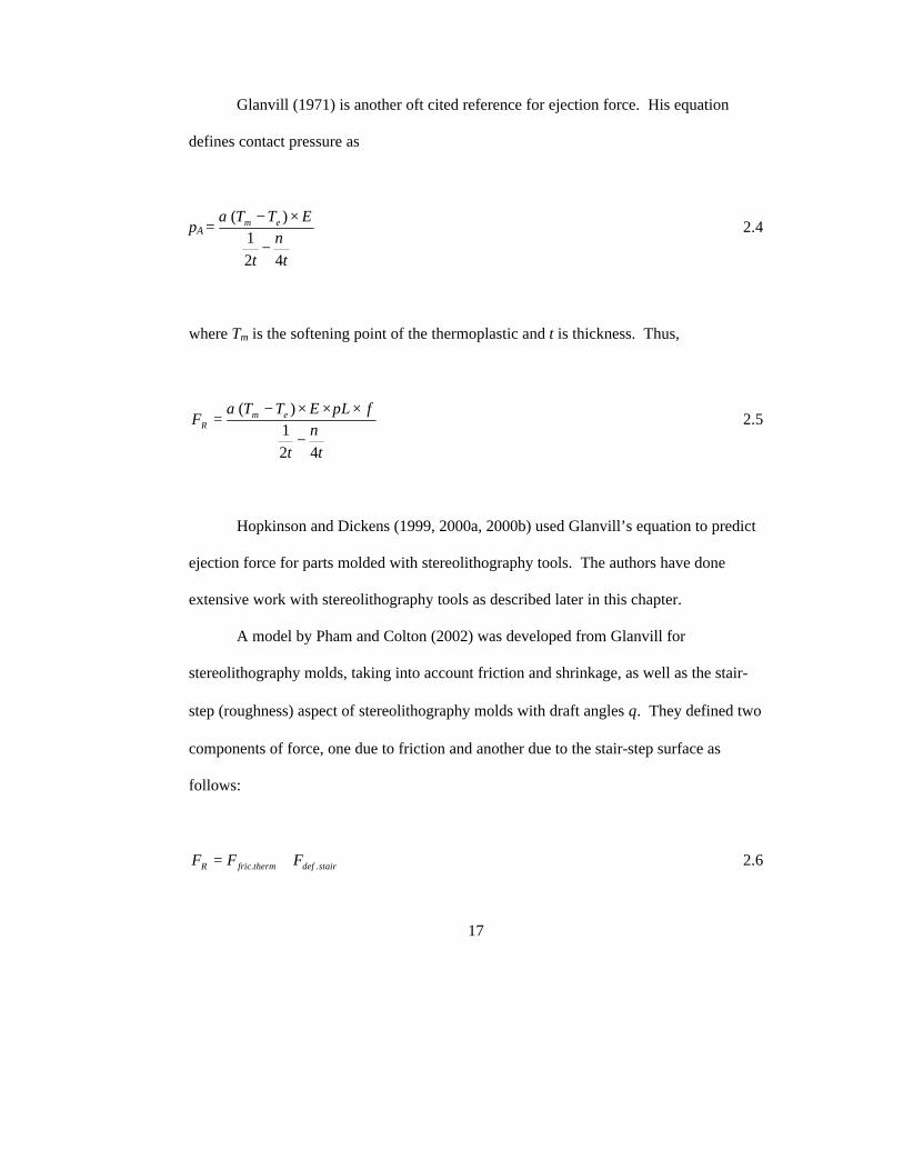
Glanvill (1971) is another oft cited reference for ejection force. His equation

defines contact pressure as

pA

tt

ETT em

421

)(ν

α

−

×−= 2.4

where Tm is the softening point of the thermoplastic and t is thickness. Thus,

tt

fLETTF em

R

421

)(ν

πα

−

×××−= 2.5

Hopkinson and Dickens (1999, 2000a, 2000b) used Glanvill’s equation to predict

ejection force for parts molded with stereolithography tools. The authors have done

extensive work with stereolithography tools as described later in this chapter.

A model by Pham and Colton (2002) was developed from Glanvill for

stereolithography molds, taking into account friction and shrinkage, as well as the stair-

step (roughness) aspect of stereolithography molds with draft angles θ. They defined two

components of force, one due to friction and another due to the stair-step surface as

follows:

stairdefthermfricR FFF .. += 2.6

18

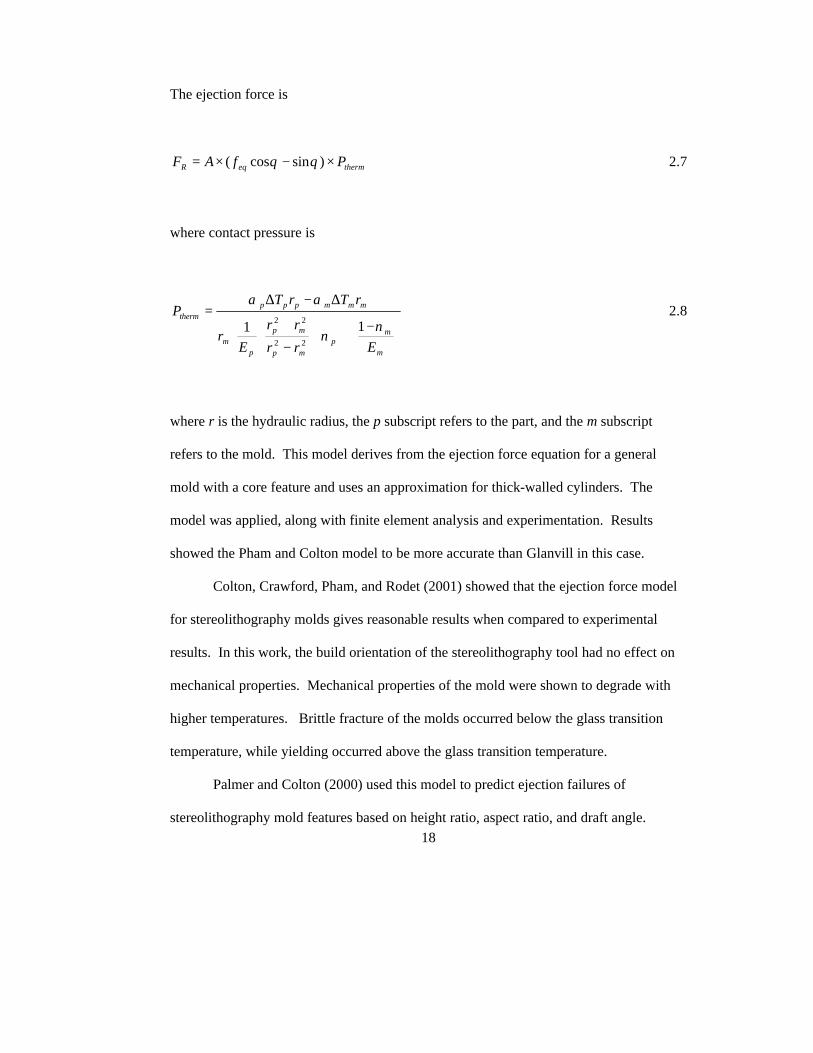
The ejection force is

thermeqR PfAF ×−×= )sincos( θθ 2.7

where contact pressure is

−+

+

−

+

∆−∆=

m

mp

mp

mp

pm

mmmppptherm

Err

rr

Er

rTrTP

νν

αα

1122

22 2.8

where r is the hydraulic radius, the p subscript refers to the part, and the m subscript

refers to the mold. This model derives from the ejection force equation for a general

mold with a core feature and uses an approximation for thick-walled cylinders. The

model was applied, along with finite element analysis and experimentation. Results

showed the Pham and Colton model to be more accurate than Glanvill in this case.

Colton, Crawford, Pham, and Rodet (2001) showed that the ejection force model

for stereolithography molds gives reasonable results when compared to experimental

results. In this work, the build orientation of the stereolithography tool had no effect on

mechanical properties. Mechanical properties of the mold were shown to degrade with

higher temperatures. Brittle fracture of the molds occurred below the glass transition

temperature, while yielding occurred above the glass transition temperature.

Palmer and Colton (2000) used this model to predict ejection failures of

stereolithography mold features based on height ratio, aspect ratio, and draft angle.

19

Height ratio was the most critical factor in determining feature life, while aspect ratio had

no conclusive effect. As expected, larger draft angles increased feature life. Fatigue-

based chipping failures also occurred.

Cedorge and Colton (2000) studied the stair step effect of stereolithography tools.

Surface roughness resulting from the stereolithography build process depended on layer

thickness and draft angle. The authors showed a trade-off between these two parameters

in terms of ejection force. For tools built with thin layers, ejection force decreased with

draft angle, while for thick layers, ejection force increased with draft angle.

Colton and LeBaut (2000) showed that ejection force decreases with number of

shots in a stereolithography mold. This was because the mold gradually heated up, and

shrinkage was less because the mold and part temperatures were closer together. The

authors also found that the stereolithography material continued to cure and become

harder.

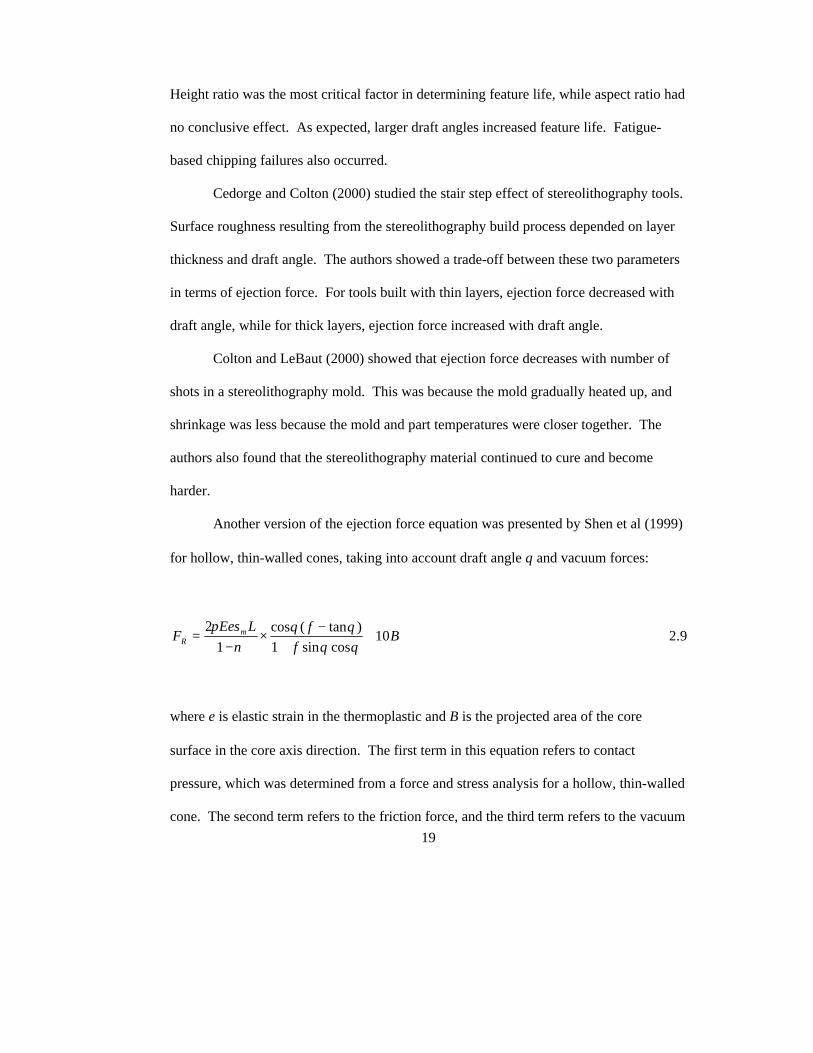
Another version of the ejection force equation was presented by Shen et al (1999)

for hollow, thin-walled cones, taking into account draft angle θ and vacuum forces:

Bf

fLsEF m

R 10cossin1

)tan(cos1

2+

+−

×−

=θθθθ

νεπ

2.9

where ε is elastic strain in the thermoplastic and B is the projected area of the core

surface in the core axis direction. The first term in this equation refers to contact

pressure, which was determined from a force and stress analysis for a hollow, thin-walled

cone. The second term refers to the friction force, and the third term refers to the vacuum

20

force. Experiments by Shen, et al showed agreement with model results, though molding

parameters were not discussed.

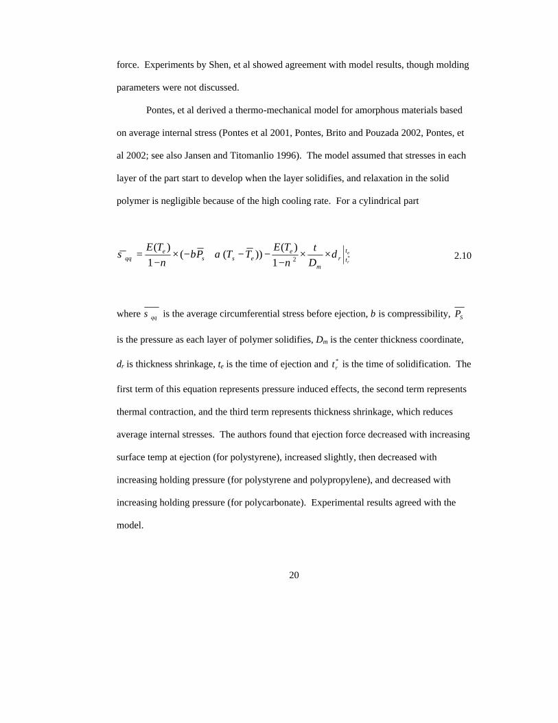
Pontes, et al derived a thermo-mechanical model for amorphous materials based

on average internal stress (Pontes et al 2001, Pontes, Brito and Pouzada 2002, Pontes, et

al 2002; see also Jansen and Titomanlio 1996). The model assumed that stresses in each

layer of the part start to develop when the layer solidifies, and relaxation in the solid

polymer is negligible because of the high cooling rate. For a cylindrical part

e

r

ttr

m

eess

e

DtTE

TTPTE

*21)(

))((1

)(δ

ναβ

νσ θθ ××

−−−+−×

−= 2.10

where θθσ is the average circumferential stress before ejection, β is compressibility, SP

is the pressure as each layer of polymer solidifies, Dm is the center thickness coordinate,

δr is thickness shrinkage, te is the time of ejection and *rt is the time of solidification. The

first term of this equation represents pressure induced effects, the second term represents

thermal contraction, and the third term represents thickness shrinkage, which reduces

average internal stresses. The authors found that ejection force decreased with increasing

surface temp at ejection (for polystyrene), increased slightly, then decreased with

increasing holding pressure (for polystyrene and polypropylene), and decreased with

increasing holding pressure (for polycarbonate). Experimental results agreed with the

model.

21

Kabanemi, et al (1998) derived a numerical model for prediction of residual

stresses, shrinkage and warpage for thin, complex injection molded products. Wang,

Kabanemi, and Salloum (1997, 2000) presented the numerical approach to predict

ejection force from mold-part constraining forces and friction forces. It included finite

element thermoviscoelastic solidification analysis to account for stress and volume

relaxation of polymers under cavity-constrained conditions, and predicted distribution of

ejection force among ejector pins. The model worked well for a rigid polymer

(polycarbonate), but HDPE had significant post-molding shrinkage and warpage that was

not taken into account.

Several examples of research using models for injection force have been

described in this section. Many researchers have used the Menges or Glanvill models,

while others have derived their own models. Much of this work has shown the effects of

various parameters on ejection force and has illustrated the many different variables that

need to be taken into account. The present work follows up on these ideas by

determining the effects of three parameters on ejection forces for three mold insert

materials and two thermoplastic materials, and by applying an existing ejection force

models (from Menges) and comparing the results to experimental values. The present

work is unique in that it includes three different injection mold inserts in the same

experiment, and two of these are made by rapid prototyping processes. It is also unique

in that it includes values for modulus at temperature, standard measurements of

coefficients of friction at elevated temperatures, and near real time measurements of part

diameters (to determine shrinkage and part thickness).

22

2.1.2 Shrinkage

An important aspect of the above ejection force models is shrinkage of the

thermoplastic part. Shrinkage influences the contact pressure of the part against the core

and can affect strain and friction. The extent of shrinkage that occurs depends on

material properties and process conditions. The following works, most by researchers

previously mentioned, address shrinkage in the context of thermoplastic injection

molding and ejection forces.

Malloy and Majeski (1989) explained aspects of shrinkage that relate to the

injection molding process. They stated that shrinkage values for thermoplastics are often

given in ranges because they vary both parallel and perpendicular to flow and with

process conditions. Standard shrinkage values, however, have limited value in

determining ejection forces since ejection is normally at elevated temperatures. Deep

gates, long holding times, and high holding pressures in the injection molding process

can compensate for shrinkage of the part. In calculating the ejection force, accurate

values of the coefficient of thermal expansion may not be available since it is a function

of temperature and pressure in the process. Therefore, shrinkage (strain) values can be

used instead.

Burke and Malloy (1991) stated that shrinkage results from thermal contraction

and directional distortion. Thermal contraction is due to atomic vibration in which atoms

move closer together at lower energy levels, and directional distortion results from

orientation of polymer molecules during flow, and their subsequent relaxation back to a

23

coiled state after flow ends. Shrinkage is greatly influenced by ejection temperature, is

material dependent, and varies for amorphous and semicrystalline polymers.

Semicrystalline materials exhibit greater shrinkage due to phase transformation of the

crystalline portion: random amorphous coils and high free volume in the melt reduce to

orderly packed chains in the crystal lattice. Amorphous polymers, on the other hand,

contract much more gradually.

Michaeli et al (1999) modeled the development of material properties and

crystallization due to processing. They found that the temperature at which the

crystallization peak occurs decreases, and the crystallization interval widens, with

increasing cooling rate. That is, crystallization starts earlier at lower cooling rates.

Menges, et al (2001) stated that, for both amorphous and crystalline

thermoplastics, holding pressure exerts the greatest effect on shrinkage (degressive

effect) in the injection molding process. The temperature of the material is the second

major factor influencing shrinkage. Higher temperature results in higher thermal

contraction potential, but also lowers viscosity for better pressure transfer. With a longer

holding time, the effect of improved cavity pressure predominates for crystalline

materials. Menges et al provided shrinkage values for some thermoplastics, but stated

that the best data are found through experience.

Pantani and Titomanlio (1999) found that higher pressure histories inside the

injection mold cavity – obtained by increasing either holding time or holding pressure –

result in a lower final shrinkage and in a delayed start of shrinkage inside the mold for a

polystyrene plate.

24

In mold experiments with polycarbonate, Pontes et al (2001) found that increasing

holding pressure reduces contact pressure by decreasing diametrical shrinkage. Holding

time, however, had no effect on the shrinkage due to fast solidification of this material.

In their ejection force modeling work, the authors described average circumferential

stress to include volumetric shrinkage due to thermal contraction (and crystallization) and

thickness shrinkage, which reduces stress. Ejection force, then, depended on elastic

modulus, friction coefficient, part thickness, and variation of the volumetric shrinkage.

In their model, initially, ejection force increased (or plateaued) with increasing holding

pressure because of thickness shrinkage, while at higher holding pressures a reduction in

volumetric shrinkage reduced ejection force.

As indicated by the research described in this section, shrinkage varies with

parallel and perpendicular flow, injection and ejection temperature, holding pressure and

time, material structure and properties, and pressure histories. In the present work, while

shrinkage is not analyzed directly, it is measure and used in the Menges model to

calculate ejection force. Shrinkage influences the contact pressure of the part on the core

(see Chapter 3). Furthermore the effects of cooling time, packing pressure, and packing

time on ejection force are determined in part by the shrinkage characteristics of the

thermoplastic material.

25

2.1.3 Friction and Adhesion

Friction is another important aspect in determining ejection forces. Friction

between the thermoplastic part and the injection mold core not only depends on the

mechanical relationship between the two surfaces, but also on an adhesive component

inherent in the properties of the two materials at processing conditions. The following

works address friction and adhesion, some in general terms, others specifically as they

apply to polymers and injection molding.

Contact between two solids occurs only at asperities (ed. Eley 1961, Ch. V).

Extremely high pressures are produced at these contact points and, in metals, plastic flow

occurs. Under plastic conditions, the area of real contact is directly proportional to the

load and is independent of the apparent area of contact. During sliding at slow speeds,

with no temp increase, fragments of one metal can strongly adhere to the other (cold

welding). The frictional force is then the force required to shear the junctions formed in

this way.

With softer metals junctions are more ductile and easily deformed, and

appreciable adhesion may occur. Relatively smaller adhesions occur in plastics due to

higher elastic recovery. Adhesion may thus occur by reducing elastic stress or by

increasing ductility.

A number of concepts relating polymer friction and adhesion to thermoplastic

injection molding (with steel molds) were presented by Burke and Malloy (1991) and are

summarized below. More on friction and adhesion theory is presented in Chapter 3.

26

• Plastics have relatively low modulus values, which lead to frictional values that

are not always directly proportional to load. This is attributable to adhesion and

deformation.

• Theoretical calculations show that van der Waals forces, which attract molecules

with permanent dipoles, and London dispersion forces, which cause dipoles

created by motion of electrons in the molecule, are great enough to produce bonds

exceeding the cohesive strength of most adhesives.

• In the surface energy theory, a liquid may wet and spread over a solid surface if

the critical surface tension of the solid is greater than that of the liquid. Heat

decreases viscosity and improves wettability; heat and pressure promote wetting

and spreading. Molten polymers on steel under injection molding conditions are a

good environment for wetting and spreading.

• Wetting and spreading does not necessarily imply adhesion. Apparently both

physical adsorption and surface energy criteria must be met for adhesion to occur.

An increase in adhesion will increase the apparent coefficient of friction, which

depends on the specific polymer-steel combination.

• Surface roughness causes mechanical coupling and increases surface area over

which van der Waals forces can act. Imperfect surfaces lead to inherent voids or

trapped gas bubbles and imperfect molecular fit, limiting the bond strength.

• The coefficient of static friction increases with increasing surface roughness,

depending on viscosity and pressure applied. A highly viscous material under

low pressure may not wet the steel. The direction of polishing affects part

27

ejection. The coefficient of friction decreases with increasing cooling time

because shrinkage decreases the mechanical anchorage of the polymer, i.e., it no

longer completely penetrates irregularities in the mold.

Looking at polymer adhesion from the standpoint of wear, Briscoe (1981)

summarized several fundamental aspects, including cohesive wear and interfacial wear.

Cohesive wear mechanisms occur adjacent to the interface, e.g., abrasion and fatigue

wear induced by tractive stresses. Interfacial wear processes dissipate frictional work in

much thinner regions and at greater energy densities, e.g., transfer wear and chemical or

corrosive wear. In interfacial wear, frictional work originates from adhesive forces

emanating from the contacting solids. These forces generate localized plastic surface

deformation and transfer of relatively undegraded polymers to the counterface in certain

systems.

Also discussed in this paper is natural adhesive or transfer wear, specifically,

initial adhesion. Briscoe stated that initial junction strength is a function of the

interaction of surface forces and mechanical properties of the contact. For polymers, the

surface forces consist of van der Waals, coulombic and possibly hydrogen bonding

forces. The higher the surface free energy of the polymer, the greater the adhesive force.

Polymers above the glass transition temperature will adhere more strongly because they

conform to surface imperfections and have a relatively low level of stored elastic strain.

Very clean metal surfaces may promote chemical bonding. Essentially brittle and highly

28

elastic crosslinked polymers tend to fail at the interface. This includes polymers below

the glass transition temperature and crosslinked systems.

Czichos (1983, 1985) investigated contact deformation, static friction, and

tribological behavior of polymers. In his work contact deformation was measured for

four crystalline thermoplastics in loading and unloading conditions. A model was

proposed that takes into account elastic, viscoelastic, and viscoplastic components.

Polymer to polymer coefficients of friction were measured, using a pin-on-disc

configuration, and plotted against sliding distance. Experimental frictional work was

plotted against the work of adhesion using the Dupre equation (see Chapter 3), showing

that a reasonable correlation exists. Also, coefficient of friction and wear rate were

plotted against surface roughness for four polymers against steel. The author found that

adhesion was the primary influence for very low surface roughness, while abrasion was

the primary influence for higher roughness.

Benabdallah and Fisa (1989) measured the static friction coefficient between a

steel surface and three thermoplastics with surface roughnesses varying between 0.4 µm

RMS to 40.5 µm RMS. Parameters measured were normal load, relative displacement

and tangential force. In these tests, static coefficient of friction decreased with increasing

normal loads ranging up to 160 N. This is explained by an increasing influence of the

adhesion component of friction. Also, the friction coefficients decreased with increasing

surface roughness since, with smoother surfaces, there is more adhesion. The authors

present a model for friction coefficient µs based on this work:

29

µs = αFNn 2.11

where FN is normal load, α is a proportionality constant that depends on polymer surface

roughness and n is experimentally determined for each polymer.

Benabdallah (1993) investigated static shear strength during contact between a

bulk plastic and a metallic plate, both with smooth surfaces. The experimental equipment

included one apparatus to measure static friction force and another to measure the real

area of contact. The adhesion component of friction was approximated by the measured

static friction force. The author determined bulk shear strength of plastics experimentally

following ASTM D732-78 and found surface energies from the Young equation (see

Chapter 3). In this work the friction force was assumed to consist only of the adhesion

component due to the smoothness of the contacting surfaces. That is, the deformation (or

ploughing) component was not considered. Friction force equaled the maximum

tangential load, which corresponded to the minimum force required to initiate motion.

The paper includes plots of the adhesion component of friction against the calculated

work of adhesion according to the Dupre equation, ( ) 21

212 γγφ=aW , where the

interaction parameter, φ, equals 1, and the static shear strength against the real contact

pressure (the ratio of applied load and real area of contact).

Benabdallah then combined the Young equation with the geometric mean

equation to obtain:

30

( )( )

( ) ( ) 212

1

21

21

2

cos1 dSd

L

pLp

SdL

L γγγ

γγ

θγ+

=

+ 2.12

This equation is in the form y = mx+b. Given known surface energies of six liquids,

contact angles were measured and x and y plotted. Then the square of the intercept

determined the dispersion component, the square of the slope determined the polar

component, and the addition of the two gave the total surface energy of the solid γs.

The author concluded that the adhesion component of friction increases with the

real area of contact and is large when the surface energy of the plastic material is high. It

was also found that a correlation may exist between the adhesion component of friction

and the work of adhesion when evaluated as a function of the real area of contact.

Menges and Bangert (1981) measured static coefficients of friction for

determining opening and ejection forces in injection molding. This work looks at the

effects of various parameters, including surface (contact) pressure, cooling time, mold

temperature, holding pressure, and surface roughness. Various thermoplastics were

studied, but results were reported only for polypropylene. In all cases, the friction

coefficient decreased with surface roughness in the range 1 to 35 microns. In general the

friction coefficient also decreased with increasing cooling time. The effects of other

parameters were varied. The friction coefficient results varied from standard

measurements for polypropylene.

Balsamo, Hayward and Malloy (1993) conducted studies on ejection forces and

coefficients of friction. The authors found, first, that external lubricants have a large

31

effect on ejection force. They also measured static friction coefficients for polystyrene,

polypropylene, a polycarbonate/polyethylene alloy, and filled polycarbonate parts on

nickel, steel, and polytetrafluoroethylene (PTFE)/nickel plated mold cores. While noting

that the friction test does not exactly duplicate the injection molding environment, they

found that friction coefficients are generally lowest on PTFE/nickel surfaces and highest

on steel surfaces. Some coefficients changed significantly with temperature.

In Dearnley’s work (1999) to study low friction surfaces for injection molds, steel

rings were coated with TiN (polished), CrN (polished and spark eroded), and MoS2

(polished and spark eroded) and used as a core around which an acetal ring was molded.

Coating thickness, surface hardness, and surface roughness were measured, and friction

force was determined experimentally. Spark eroded surfaces were found to have higher

roughness values and higher friction forces compared to polished surfaces. The author

attributed this to mechanical interlocking. Polished CrN had the lowest friction forces

even though polished TiN and MoS2 had lower roughness values. This was attributed to

possible differences in chemical behavior at the interface, e.g., lower surface energy (or

wettability) of CrN coatings.

Pontes et al (1997) studied the effects of processing conditions on ejection forces

for tubular moldings. Parameters included surface roughness, injection temperature and

holding pressure. Two thermoplastics were used, one amorphous and one crystalline.

For polyphenylene ether (PPE), ejection force increased with injection temperature and

decreased with holding pressure, as would be expected. For polypropylene, ejection

force decreased initially with surface roughness (less than 0.75 microns), then increased.

32

For polypropylene, ejection force decreased as injection temperature increased, indicating

that the core surface temperature was different than ejection temperature, and that

deformation ability increased with higher temperature. For polypropylene, ejection force

decreased with increasing holding pressure, as was expected. The diametrical shrinkage

was determined from shrinkage at room temperature and the coefficient of thermal

expansion. Calculated values for the equivalent coefficient of friction of PPE

(amorphous) were near the lower range of published values. The authors concluded that

adhesion appears to be an important factor for semicrystalline materials molded on

surfaces with low surface roughness.

Sasaki et al (2000) molded cylindrical parts with polypropylene, polymethyl

methacrylate (PMMA), and polyethylene terephthalate (PET) at a range of surface

roughnesses from 0.016 to 0.689 microns Ra. In all cases, ejection force increased

significantly when surface roughness approached zero. Optimum surface roughness (in

terms of ejection force) for polypropylene and PET was approx. 0.2 microns and for

PMMA was 0.009 microns. For lower values of roughness, the meniscus force or van der

Waals force was thought to be the greatest factor, whereas for higher values of roughness,

the “engraving or scratching” of the surface came into play. Ejection force was also

measured on polypropylene and PET parts from cores with various coatings. Here,

tungsten carbide/carbon coating was found to be most effective for reducing ejection

force. TiN (HCD), TiN (Arc), DLC, and CrN coatings also showed ejection force

reduction effects.

33

Ferreira et al (2001) friction tested polycarbonate and polypropylene using a

special prototype apparatus. The testing procedure included heating the specimens to

processing temperatures, applying a normal load (so that the specimen replicated the

mold surface), cooling to ejection temperature, then pulling the specimen. At room

temperature, the coefficient of friction of polycarbonate at 0.32 was similar to published

values at 0.31. At high temperature, the coefficient was much higher at 0.47. For

polypropylene at high temperature, the coefficient of friction was 0.19, much lower than

published values, 0.36. A similar approach to imprinting the mold surface onto the

specimens was used in the standard friction tests in the present work (see Chapter 4).

In related work, design of experiments was used to determine the effect of polish

direction, surface roughness, and temperature on the coefficient of friction (Ferreira et al

2002). Results showed that testing temperature and surface roughness had a significant

effect on the coefficient of friction for polycarbonate. For polypropylene, none of the

parameters had a significant effect on the coefficient, except possibly the interaction of

polish direction and roughness. Friction values for both polymers were higher than

published values.

Muschalle (2001) measured the coefficient of friction for polycarbonate

(amorphous) and polypropylene (semi-crystalline) materials against steel with two

different surface roughnesses, machining directions, and temperatures. Results showed

that the friction coefficient for polycarbonate was higher at higher temperature, while that

for polypropylene was lower at higher temp. Also, the coefficient for polypropylene was

34

higher when temperature and pressure caused surface reproduction of the metal on the

plastic.

The works described in this section indicate the many aspects of friction, which

includes both a mechanical and an adhesive component. No unifying theory seems to

exist for friction, but, rather, it can be explained by one or another or a combination of

concepts. This can be seen in the friction testing in the present work, where coefficients

of static friction are influenced by adhesion and/or mechanical components of friction to

varying degrees (reference Chapters 5 and 6).

2.2 Rapid Tooling

2.2.1 Background

One of the most promising techniques for low volume, net shape manufacturing

tools is rapid tooling, i.e., the application of rapid prototyping processes for the purpose

of making tools. Rapid tooling processes are additive and produce a tool or pattern from

a CAD model. Direct rapid tooling processes generate the tool itself from the CAD file,

while indirect rapid tooling processes require intermediate steps and usually generate a

pattern from which a tool is made. A wide range of materials can be used in rapid tooling

processes, from waxes and resins to ceramics and metals. Those processes that use metal

materials and build tools directly tend to be more suitable for production tools. These

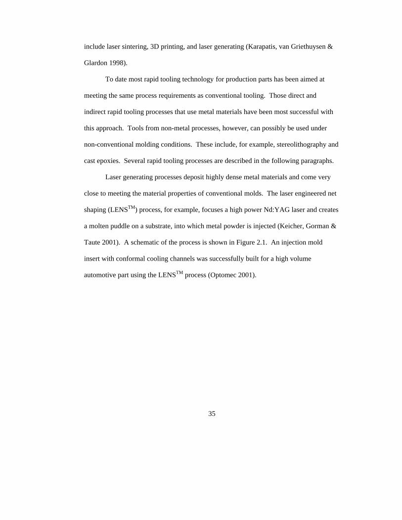
35

include laser sintering, 3D printing, and laser generating (Karapatis, van Griethuysen &

Glardon 1998).

To date most rapid tooling technology for production parts has been aimed at

meeting the same process requirements as conventional tooling. Those direct and

indirect rapid tooling processes that use metal materials have been most successful with

this approach. Tools from non-metal processes, however, can possibly be used under

non-conventional molding conditions. These include, for example, stereolithography and

cast epoxies. Several rapid tooling processes are described in the following paragraphs.

Laser generating processes deposit highly dense metal materials and come very

close to meeting the material properties of conventional molds. The laser engineered net

shaping (LENSTM) process, for example, focuses a high power Nd:YAG laser and creates

a molten puddle on a substrate, into which metal powder is injected (Keicher, Gorman &

Taute 2001). A schematic of the process is shown in Figure 2.1. An injection mold

insert with conformal cooling channels was successfully built for a high volume

automotive part using the LENSTM process (Optomec 2001).

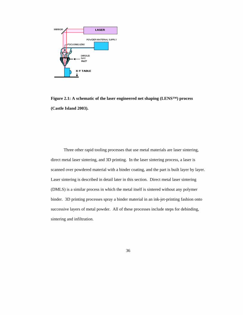
36

Figure 2.1: A schematic of the laser engineered net shaping (LENS™) process

(Castle Island 2003).

Three other rapid tooling processes that use metal materials are laser sintering,

direct metal laser sintering, and 3D printing. In the laser sintering process, a laser is

scanned over powdered material with a binder coating, and the part is built layer by layer.

Laser sintering is described in detail later in this section. Direct metal laser sintering

(DMLS) is a similar process in which the metal itself is sintered without any polymer

binder. 3D printing processes spray a binder material in an ink-jet-printing fashion onto

successive layers of metal powder. All of these processes include steps for debinding,

sintering and infiltration.

37

Stereolithography, like laser sintering, employs a scanning laser, but uses liquid

resin build materials. The stereolithography process is described in detail later in this

section.

Indirect processes generate a pattern using rapid prototyping techniques, then

build a tool from that pattern. Although indirect processes have more steps, they benefit

from a wider range of material choices. At the Pennsylvania State University, a powder

metallurgy process was used to make a mold insert (Weaver et al 2000). From a three

dimensional model, a pattern was generated using a three dimensional plotting process, a

negative of the tool was cast in silicone rubber, and a slurry of steel and ceramic was cast

into the negative to make the final tool insert. Such a tool has excellent mechanical

properties and is capable of high volume production.

Another option for indirect tooling is cast epoxy, in which a blend of resin and

aluminum filler is cast over a rapid prototyped pattern. The resulting tool insert is

machineable, capable of withstanding typical molding pressures and temperatures, and

can produce low volumes of prototype or production parts.

The two rapid tooled injection mold inserts for this research were built using laser

sintering and stereolithography processes. These represent two very different processes

among the spectrum of rapid tooling techniques. While the laser sintering material is

more like conventional tool steel, the stereolithography material is unlike what you would

expect in a production tool. The two processes were chosen first for their availability,

and second based on their economic potential for producing small quantities of parts. In

the remaining paragraphs of this section, these processes will be described in detail.

38

Laser sintering is an additive layer process in which a laser melts powdered

material by cross sections to build a part. The process is versatile in that it can use any of

several powdered materials including polymers, ceramics, and metals. For the Selective

Laser Sintering (SLS®) process, developed by the University of Texas at Austin, early

processing materials included wax, polycarbonate, unreinforced nylon, and glass

reinforced nylon (McAlea et al 1995). Today metal materials can be sintered and

infiltrated for higher densities. The laser scans across each layer of metal powder coated

with a polymer binder, and fuses the binder to create the tool (Figure 2.2). Later the

“green” part is sintered and infiltrated with copper or bronze (Beaman et al 1997, Kai &

Fai 1997).

Figure 2.2: A schematic of the selective laser sintering process (Castle Island 2003).

39

The selective laser sintering process was used to make one of the injection mold

inserts for this research. This process involves a polymer-coated 420 stainless steel-

based powder, known as LaserForm ST-100, and a 3D Systems Vanguard machine. The

sintered ST-100 material was subsequently infiltrated with bronze. Specifications of the

Vanguard are shown in Table 2.1 and material properties of ST-100 are shown in Table

2.2.

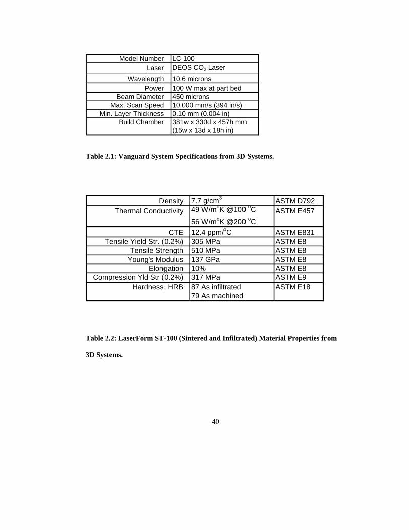
40

Table 2.1: Vanguard System Specifications from 3D Systems.

Table 2.2: LaserForm ST-100 (Sintered and Infiltrated) Material Properties from

3D Systems.

Model Number LC-100Laser DEOS CO2 Laser

Wavelength 10.6 micronsPower 100 W max at part bed

Beam Diameter 450 micronsMax. Scan Speed 10,000 mm/s (394 in/s)

Min. Layer Thickness 0.10 mm (0.004 in)Build Chamber 381w x 330d x 457h mm

(15w x 13d x 18h in)

Density 7.7 g/cm3 ASTM D792Thermal Conductivity 49 W/moK @100 oC ASTM E457

56 W/moK @200 oCCTE 12.4 ppm/oC ASTM E831

Tensile Yield Str. (0.2%) 305 MPa ASTM E8Tensile Strength 510 MPa ASTM E8

Young's Modulus 137 GPa ASTM E8Elongation 10% ASTM E8

Compression Yld Str (0.2%) 317 MPa ASTM E9Hardness, HRB 87 As infiltrated ASTM E18

79 As machined

41

When the 3-dimensional part is initially built on the Vanguard System, the laser

heats the metallic particles above the glass transition temperature of the polymer coating.

The polymer softens and deforms, then fuses with other particles at each contact surface.

The temperature is such that melting of the metal does not occur, only viscous flow of the

polymer coating. The metal powder is then bound together by the polymer to form the

“green” part. After the build is complete, the green part is removed from the machine

and excess powder is brushed away. A furnace cycle follows in a reducing atmosphere to

burn off the polymer, sinter the steel powder, and infiltrate the part with bronze.

Infiltration eliminates any voids within the steel, resulting in a fully dense part (Bourell et

al 1994, McAlea et al 1995).

Stereolithography, a non-metal process, uses a laser to scan a vat of liquid resin

and build a part layer by layer. Stereolithography resin, in direct comparison to

conventional mold steel, has vastly different mechanical and thermal properties. With

enhancement, such as a metal backing, a metal coating, or water cooling channels, a

stereolithography resin mold still underperforms an aluminum one under traditional

molding conditions (Li, Gargiulo & Keefe 2000). Nevertheless, there are several

examples of research in stereolithography tooling, as described in the next section.

Stereolithography was one of the first rapid prototyping processes to emerge, and

the 3D Systems stereolithography apparatus (SLA) was a pioneer rapid prototyping

system in the late 1980s (Kai & Fai 1997). The SLA system consists of a control

computer, a control panel, a laser, an optical system, and a process chamber. The SLA

250, appropriate for many applications, has been widely used across the globe and, in

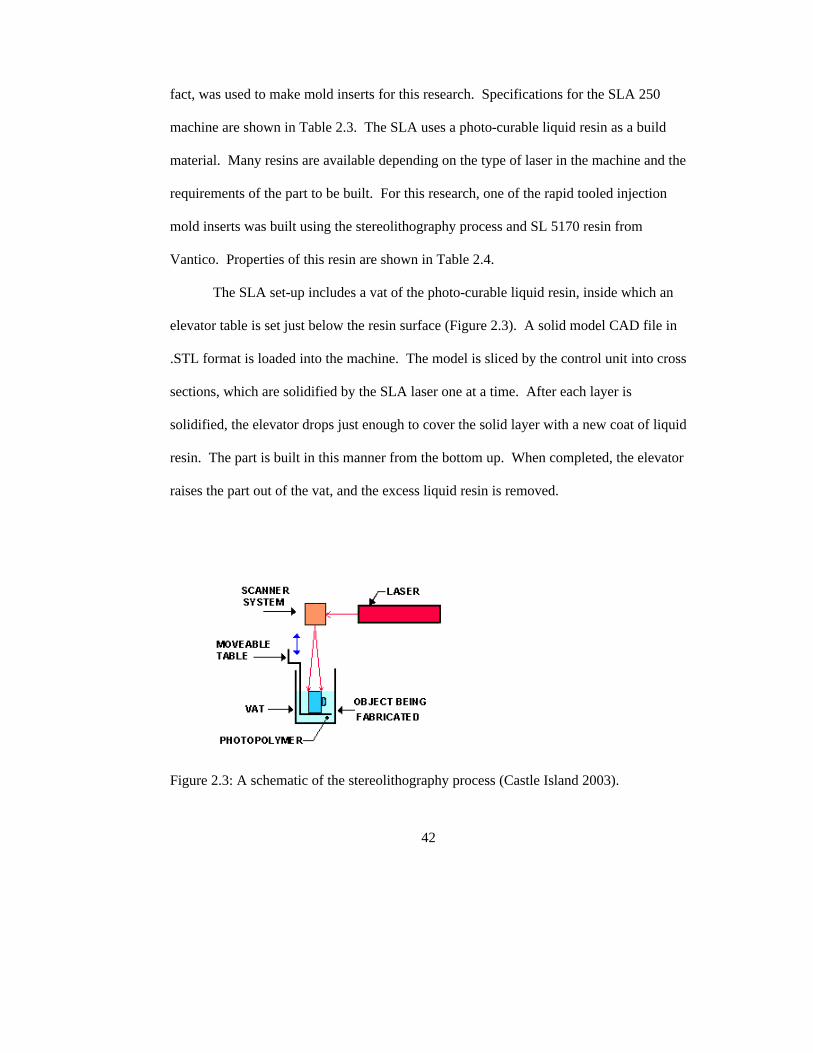
42

fact, was used to make mold inserts for this research. Specifications for the SLA 250

machine are shown in Table 2.3. The SLA uses a photo-curable liquid resin as a build

material. Many resins are available depending on the type of laser in the machine and the

requirements of the part to be built. For this research, one of the rapid tooled injection

mold inserts was built using the stereolithography process and SL 5170 resin from

Vantico. Properties of this resin are shown in Table 2.4.

The SLA set-up includes a vat of the photo-curable liquid resin, inside which an

elevator table is set just below the resin surface (Figure 2.3). A solid model CAD file in

.STL format is loaded into the machine. The model is sliced by the control unit into cross

sections, which are solidified by the SLA laser one at a time. After each layer is

solidified, the elevator drops just enough to cover the solid layer with a new coat of liquid

resin. The part is built in this manner from the bottom up. When completed, the elevator

raises the part out of the vat, and the excess liquid resin is removed.

Figure 2.3: A schematic of the stereolithography process (Castle Island 2003).

43

Table 2.3: SLA 250 System Specifications from 3D Systems.

Table 2.4: Vantico SL5170 Typical Properties (90-minute UV post cure).

Laser HeCdWavelength 325 nm

Power 24 mWBeam Diameter 0.20-0.28 mm

Max. Drawing Speed 762 mm/s

Min. Layer Thickness 0.1 mmElevator Resolution 0.0025 mm

Max. Part Weight 9.1 kgVat Capacity 32.2 L

Max. Build Envelope 250 x 250 x 250 mm

Tensile Strength 59-60 MPa ASTM D638Tensile Modulus 3737-4158 MPa ASTM D638

Elongation at Break 8% ASTM D638Glass Transition Temp 65-90oC DMA

CTE 90 ppm/oC TMA (T<Tg)

Thermal Conductivity 0.200 W/moKHardness, Shore D 85 DIN 53505

Density 1.22 g/cm3

44

The mechanisms that are the basis for the stereolithography process are free

radical and cationic photopolymerization. Polymerization is the process by which

monomers are linked into larger, chain-like molecules called polymers. Further linking

leads to the crosslinking of these chains. In free radical polymerization, heat or light

energy decomposes an initiator to generate free radicals that catalyze the polymerization

process. In cationic photopolymerization, cationic photoinitiators cause reactions that

open molecular ring structures to catalyze the polymerization process. Free radical

photopolymerization is associated with acrylate resins, and cationic photopolymerization

is associated with epoxy resins.

The resins used in the 3D Systems’ SLA machines are UV-curable photopolymers

made up of photoinitiators and reactive liquid monomers. In the SLA polymerization

process, sufficient crosslinking is required to prevent the polymer molecules from

dissolving back into monomers. Furthermore, since the cured resin must withstand forces

during recoating, the polymer molecules must be sufficiently strong. Increasing the laser

power results in a higher polymerization rate and thus a faster build rate, but brittleness

also results, due to lower molecular weight. Cure depth must be deep enough to prevent

delamination, but not so deep as to cause distortion and, therefore, inaccurate parts (Kai

& Fai 1997, Beaman et al 1997).

2.2.2 Stereolithography and Laser Sintering for Injection Molding Tools

Rapid tooling processes lend themselves well to injection molds because of their

ability to generate complex shapes as easily as simple ones. Complex shapes that are

45

difficult or impossible to machine, detailed internal structures, and thin walls can be

readily generated. This allows the integration of conformal cooling channels within the

mold, which lower residual thermal stresses and can reduce cycle times (Sachs et al

2000). Some rapid prototyping processes have the ability to vary material composition

during fabrication. This local composition control benefits rapid tooling because it

allows tailoring of various material properties, such as conductivity, corrosion resistance,

and hardness (Cho, Sachs, & Patrikalakis 2001). It is theoretically possible, for example,

to build an injection mold with a core of highly conductive material, such as copper, and

surround it with a wear resistant material, such as stainless steel. Rapid tooling processes

lend themselves well to low volume production because they reduce the requirements for

labor intensive machining, minimize material waste, and, in some cases, use less

expensive materials. Thus they have the potential to reduce tooling costs enough to make

low volume injection molding economically feasible.

Research in the area of rapid tooling for injection molding is varied. The work

described in section 2.1.1 includes some research with rapid prototyped tools. Additional

work specifically pertaining to stereolithography and laser sintering, is summarized

below.

Laser sintering uses powdered metals for tooling and is not as challenging as

stereolithography in terms of strength and thermal conductivity, so there are more

examples of its use for injection molding prototyping in industry (e.g., Campbell 2000).

Laser sintering with copper polyamide has been used to build small, low volume mold

inserts, such as those for a brake reservoir and a glass guide (Nelson et al 1998). In these

46

cases, the advantages of laser sintering included durability for up to hundreds of parts,

low cost and lead time, and cycle times that are comparable to those with conventional

tools.

Pham, Dimov and Lacan (2000) studied characteristics related to laser sintered

tool accuracy, including shrinkage of the tool material and finishing requirements. Mold

insert accuracy requires fine tuning of scaling and offset factors due to shrinkage and

careful planning of tool finishing processes. Two case studies indicate successful use of

laser sintering for injection molding and gravity die casting. In cases for two injection

molded parts, Dalgarno and Stewart (2001) studied cycle time effects of conformal

cooling and molding costs based on tool durability, and compared laser sintered tool

results with conventional tooling. Due to tool finishing requirements, they found no lead

time advantage for the laser sintered tooling process. The laser sintered tools, however,

did exhibit cycle time savings with conformal cooling channels and economic benefits at

low demand rates. Other work includes optimization of shapes for heating and cooling

lines in mold inserts made with the direct metal laser sintering process (commercialized

by EOS), which sinters bronze particles and infiltrates with epoxy resin (Hopkinson &

Dickens 2000a).

Hopkinson and Dickens have investigated stereolithography tools for injection

molding, including tool failure, tool strength and ejection force. In a comparison of

stereolithography with aluminum injection mold tooling, they found that the low thermal

conductivity can be advantageous since the tool surface stays above its glass transition

temperature for easier ejection. Also, tool degradation due to thermal cycling is reduced,

47

and the ability to mold long thin slots is enhanced. Ejection forces in this work were

calculated using the equations developed by Glanvill and Menges et al (Hopkinson &

Dickens 2000b).

In other work, models were developed to predict tool strength and ejection force

(Hopkinson & Dickens 2000c, 2000d). Heat transfer through the tool was measured and

modeled. Then the results of the heat transfer analysis were used in a finite element

analysis model to predict tool strength. The model showed a decrease in tool strength

with increased cooling time before ejection. Ejection forces were predicted based on a

modified equation by Glanville and Denton. Longer cooling times were found to lead to

higher ejection forces, as expected, due to part shrinkage onto the core. The predicted

values, however, were approximately 30 percent lower than actual values, and the

measured values contained some inherent variation.

Harris and Dickens (2001) explored two design variables for stereolithography

injection mold inserts, namely, layer thickness and draft angle. They found that ejection

forces increase with increasing stereolithography layer thickness and decreasing draft

angles, thus increasing the risk of mold breakage. Interestingly, the linear changes in

these two variables cause nonlinear changes in the ejection force, suggesting that

optimum values must be found that balance ejection force requirements with desired part

design and economy of stereolithography process. A later paper describes their study of

the morphology of thermoplastic materials injection molded from stereolithography and

aluminum tools (Harris & Dickens 2003). Parts from the stereolithography tool had

longer cooling times and higher crystallinity. Experimental work demonstrated that

48

crystallinity can be controlled by using a nucleating agent or by adjusting melt

temperature.

The work of Dickens and Rudgley (2001) demonstrates the successful use of

stereolithography resin inserts to mold an engineering polymer. With much lower

injection pressure, speed, and clamping force, poly ether ether Ketone (PEEK), an

engineering polymer, was injected into a room temperature stereolithography mold insert.

The low thermal conductivity of the insert allowed the mold to fill completely at the

lower pressure level. The part was ejected at a higher temperature so that the insert

flexed during ejection. The part was molded successfully, and the slower cooling

resulted in higher crystallinity as compared to parts molded in a conventional tool.

2.2.3 Summary

There are many rapid prototyping processes in use or under development today,

some of which have been described in this section. A subset of the rapid prototyping

processes can be applied to make tools, including injection mold inserts. The present

work investigates tools from two of these processes, laser sintering and stereolithography.

Laser sintering with powdered metal has been successfully used to build injection molds

for limited quantities of parts. Stereolithography with epoxy resin has been the subject of

research for injection mold inserts, but has not been used for production to any significant

extent. This work follows up much of the work described previously in this section by

taking a systematic look at inserts from these two processes for molding two different

thermoplastic materials. Ejection forces and friction coefficients are measured, compared

49

with model-based calculations, and baselined against a machined steel insert. The data

collected help to determine the applicability of these rapid tools to injection molding, at

least in terms of their ability to withstand the forces of ejection.

50

CHAPTER 3

THEORY

This chapter includes necessary theoretical background on polymeric materials,

the coefficient of friction, and an ejection force model. First amorphous and crystalline

aspects of the thermoplastic materials used in this work are presented. Some friction

theory follows, including discussions on the deformation and adhesion components of

friction. The final section derives the primary ejection force equation used in this

research.

3.1 Thermoplastic Materials

Chemical structures and some properties of the two thermoplastics used in this

work are presented in this section because they relate to the shrinkage, friction, and

strength characteristics of the materials. These characteristics explain much of the

behavior of these materials in the present work during testing and experimentation and

described in Chapters 5 and 6.

51

A thermoplastic material is a polymer that has a linear macromolecular structure

and will repeatedly soften when heated and harden when cooled. Examples of

thermoplastics include styrenes, acrylics, polyethylenes, vinyls, and nylons. A crystalline

thermoplastic has sections of crystallinity, i.e., periodic ordering of molecules, whereas

an amorphous thermoplastic lacks any long range molecular order. The characteristic

differences between amorphous and crystalline polymers determine processing

parameters and influence the properties of an injection molded part.

Amorphous polymers have a second order transition, or glass transition

temperature, above which the material flows, and below which the material is glassy

(Trantina & Nimmer 1994). In general, they have lower and more uniform shrinkage,

greater post-mold stability, and high melt viscosities. Amorphous polymers also tend to

be more susceptible to chemical attack.

Crystalline polymers have a well-defined melting point below which crystals are

formed, and above which the crystals dissolve and the material flows. In general they

shrink more, and shrink more anisotropically, have low melt viscosities (long flow

lengths), and have more temperature dependent mechanical properties. Crystalline

polymers also tend to be more resistant to solvents.

3.1.1 High Impact Polystyrene

Polystyrene is a vinyl polymer (i.e., formed from hydrocarbon monomers with

double carbon bonds) having a phenyl group attached to every other carbon atom in its

hydrocarbon chain (Figure 3.1) (University of Southern Mississippi 2002). In atactic

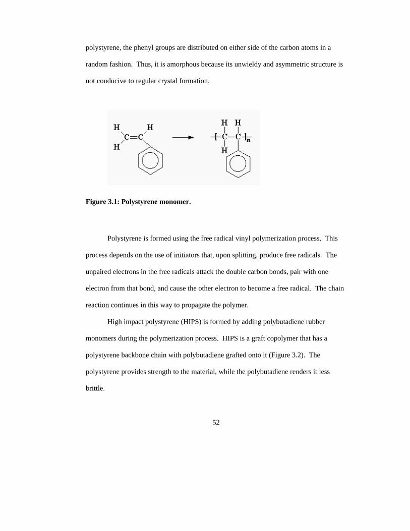
52

polystyrene, the phenyl groups are distributed on either side of the carbon atoms in a

random fashion. Thus, it is amorphous because its unwieldy and asymmetric structure is

not conducive to regular crystal formation.

Figure 3.1: Polystyrene monomer.

Polystyrene is formed using the free radical vinyl polymerization process. This

process depends on the use of initiators that, upon splitting, produce free radicals. The

unpaired electrons in the free radicals attack the double carbon bonds, pair with one

electron from that bond, and cause the other electron to become a free radical. The chain

reaction continues in this way to propagate the polymer.

High impact polystyrene (HIPS) is formed by adding polybutadiene rubber

monomers during the polymerization process. HIPS is a graft copolymer that has a

polystyrene backbone chain with polybutadiene grafted onto it (Figure 3.2). The

polystyrene provides strength to the material, while the polybutadiene renders it less

brittle.

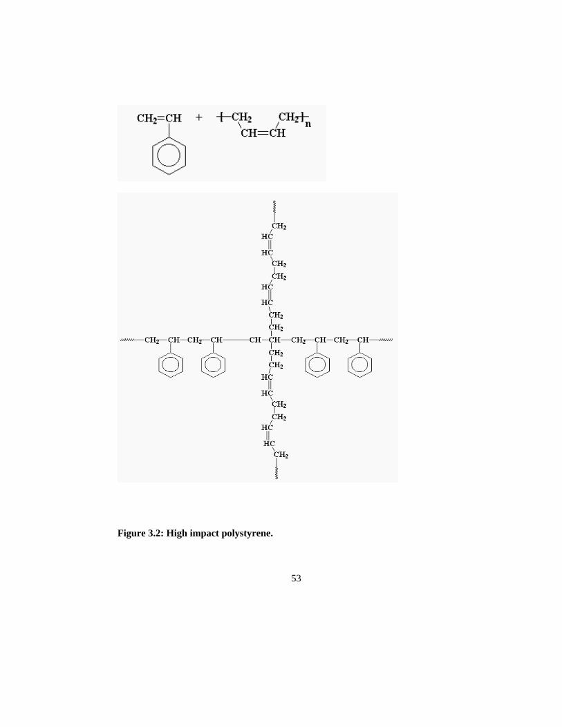
53

Figure 3.2: High impact polystyrene.

54

The HIPS material used in this work is BASF PS 495F. Its glass transition

temperature is 100 oC (212 oF). This material is more brittle at room temperature

compared to high density polyethylene. The properties of PS 495F are given in Chapter

4.

3.1.2 High Density Polyethylene

Polyethylene is also a vinyl polymer with a very simple hydrocarbon chain

(Figure 3.3). High density polyethylene (HDPE) has linear molecules (Figure 3.4) that

can pack more tightly together, as opposed to low density polyethylene that has branched

molecules. Because of its regular symmetric structure, HDPE is conducive to crystal

formation and is considered a crystalline polymer.

HDPE cannot be produced using free radical vinyl polymerization because some

termination reactions result in branching of the molecules. Instead, the Ziegler-Natta

vinyl polymerization process is used. The Ziegler-Natta process involves transition metal

catalysts and co-catalysts based on the Group III metals, and it can produce polymers of a

specific tacticity (University of Southern Mississippi 2002).

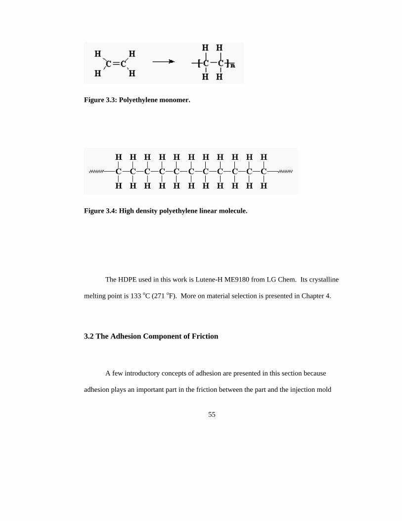
55

Figure 3.3: Polyethylene monomer.

Figure 3.4: High density polyethylene linear molecule.

The HDPE used in this work is Lutene-H ME9180 from LG Chem. Its crystalline

melting point is 133 oC (271 oF). More on material selection is presented in Chapter 4.

3.2 The Adhesion Component of Friction

A few introductory concepts of adhesion are presented in this section because

adhesion plays an important part in the friction between the part and the injection mold

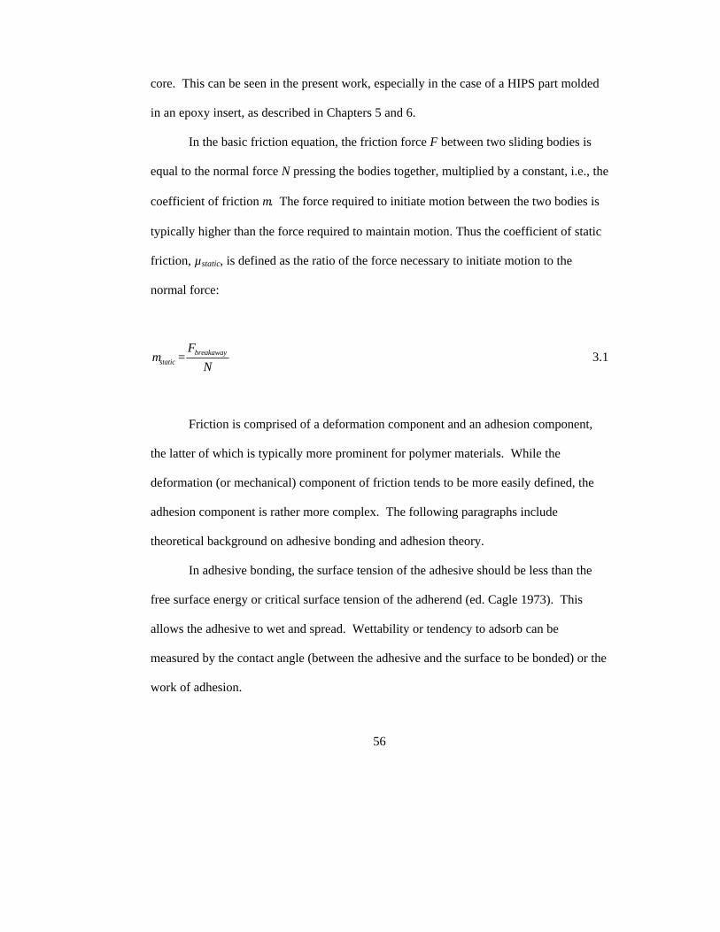
56

core. This can be seen in the present work, especially in the case of a HIPS part molded

in an epoxy insert, as described in Chapters 5 and 6.

In the basic friction equation, the friction force F between two sliding bodies is

equal to the normal force N pressing the bodies together, multiplied by a constant, i.e., the

coefficient of friction µ. The force required to initiate motion between the two bodies is

typically higher than the force required to maintain motion. Thus the coefficient of static

friction, µstatic, is defined as the ratio of the force necessary to initiate motion to the

normal force:

µstatic =Fbreakaway

N 3.1

Friction is comprised of a deformation component and an adhesion component,

the latter of which is typically more prominent for polymer materials. While the

deformation (or mechanical) component of friction tends to be more easily defined, the

adhesion component is rather more complex. The following paragraphs include

theoretical background on adhesive bonding and adhesion theory.

In adhesive bonding, the surface tension of the adhesive should be less than the

free surface energy or critical surface tension of the adherend (ed. Cagle 1973). This

allows the adhesive to wet and spread. Wettability or tendency to adsorb can be

measured by the contact angle (between the adhesive and the surface to be bonded) or the

work of adhesion.

57

Forces in the wetting and spreading phenomena include chemical bonds,

mechanical entanglement, physical and chemical adsorption, electrostatic forces of

attraction, and combinations thereof. Physical adsorption involves secondary attractive

forces, i.e., van der Waals forces: molecules with permanent dipoles, dipoles induced by

permanent dipoles in neighboring molecules (Debye forces), and London dispersion

forces. Dispersion forces are dipoles produced by the motion of electrons and are

independent of molecular polarity. Dispersion forces are considered to be the major

attractive force even when polar groups and hydrogen bonding groups are present.

Hydrogen bonding is demonstrated by molecules with hydroxyl groups.

If the critical surface tension of the solid is greater than the surface tension of the

liquid, a good bond can occur. Surface free energies of metals range from 100 to 3000

ergs/cm2, while organic liquids (including molten thermoplastics) have surface free

energies of less than 100 ergs/cm2. Heat serves to increase the ability of the adhesive to

adsorb, dissolve, and disperse. Heat also decreases viscosity, thus increasing wetting and

adsorption. Pressure and heat together improve wetting and spreading of more viscous

materials.

Some of the equations of adhesion theory that derive from surface energy are

introduced below. Surface energy or surface tension is represented by γ, where subscripts

S and L represent solid and liquid, respectively (Wu 1982). Interfacial energy is

represented by γLS. The Young equation relates contact angle θ, formed between a drop

of liquid and a solid surface, to interfacial tensions as follows:

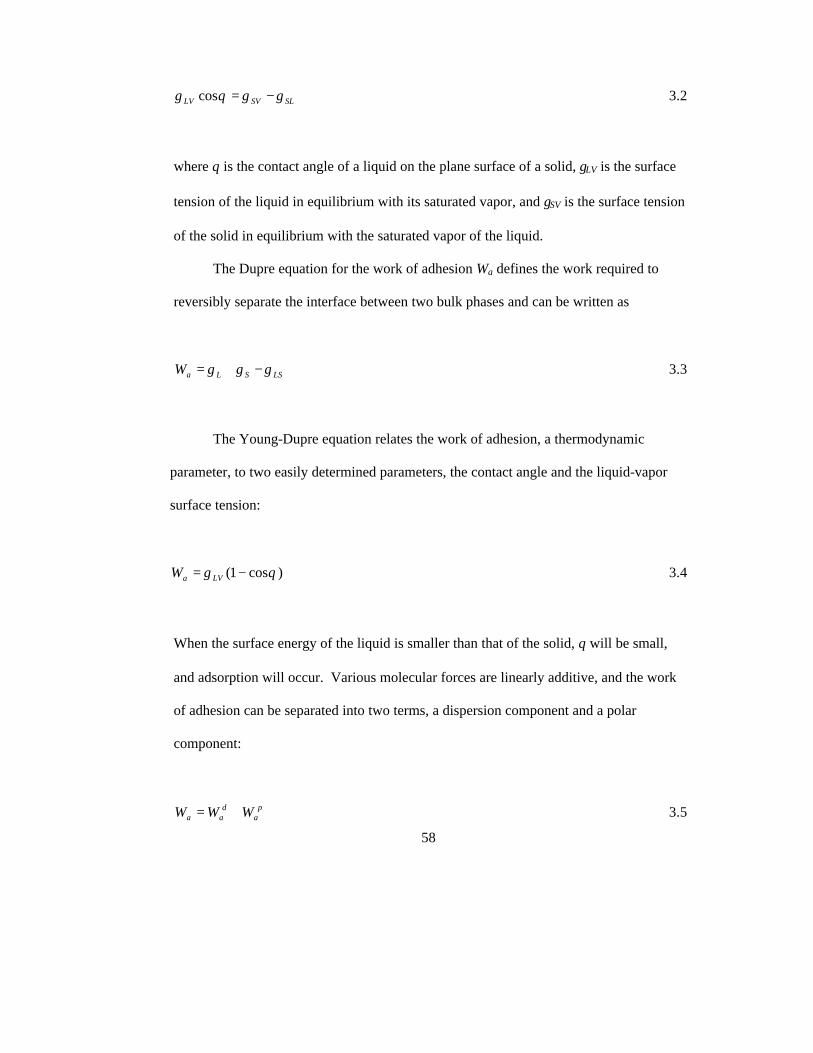
58

SLSVLV γγθγ −=cos 3.2

where θ is the contact angle of a liquid on the plane surface of a solid, γLV is the surface

tension of the liquid in equilibrium with its saturated vapor, and γSV is the surface tension

of the solid in equilibrium with the saturated vapor of the liquid.

The Dupre equation for the work of adhesion Wa defines the work required to

reversibly separate the interface between two bulk phases and can be written as

LSSLaW γγγ −+= 3.3

The Young-Dupre equation relates the work of adhesion, a thermodynamic

parameter, to two easily determined parameters, the contact angle and the liquid-vapor

surface tension:

)cos1( θγ −= LVaW 3.4

When the surface energy of the liquid is smaller than that of the solid, θ will be small,

and adsorption will occur. Various molecular forces are linearly additive, and the work

of adhesion can be separated into two terms, a dispersion component and a polar

component:

pa

daa WWW += 3.5

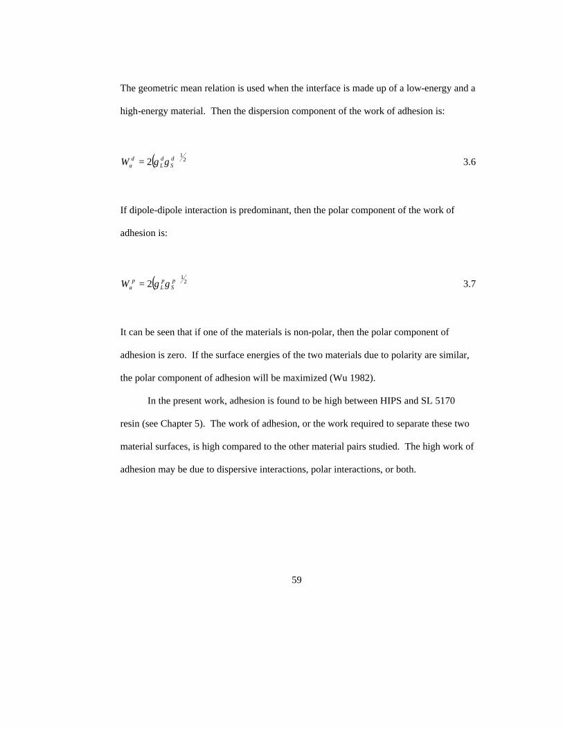
59

The geometric mean relation is used when the interface is made up of a low-energy and a

high-energy material. Then the dispersion component of the work of adhesion is:

( ) 21

2 dS

dL

daW γγ= 3.6

If dipole-dipole interaction is predominant, then the polar component of the work of

adhesion is:

( ) 21

2 pS

pL

paW γγ= 3.7

It can be seen that if one of the materials is non-polar, then the polar component of

adhesion is zero. If the surface energies of the two materials due to polarity are similar,

the polar component of adhesion will be maximized (Wu 1982).

In the present work, adhesion is found to be high between HIPS and SL 5170

resin (see Chapter 5). The work of adhesion, or the work required to separate these two

material surfaces, is high compared to the other material pairs studied. The high work of

adhesion may be due to dispersive interactions, polar interactions, or both.

60

3.3 Ejection Force Model Derivation

The ejection force model derived in this section is a key component of the present

work. It is used for theoretical comparison to experimental measurement, both for the

ejection force and the coefficient of static friction, for all the injection mold insert and

thermoplastic material combinations used.

3.3.1 Model derivation

Ejection force equations are derived from the empirical law of the friction

phenomenon, presented above, in which the friction force between two surfaces is

proportional to the normal force pressing the two surfaces together:

NF µ= 3.8

where N is the normal force and µ is the coefficient of friction, a characteristic constant

of the materials involved.

For deep parts with cores and cavities, the friction force is equal to the release

force FR, and the normal force results from the product of the contact pressure P and the

area of contact A (see Burke 1991):

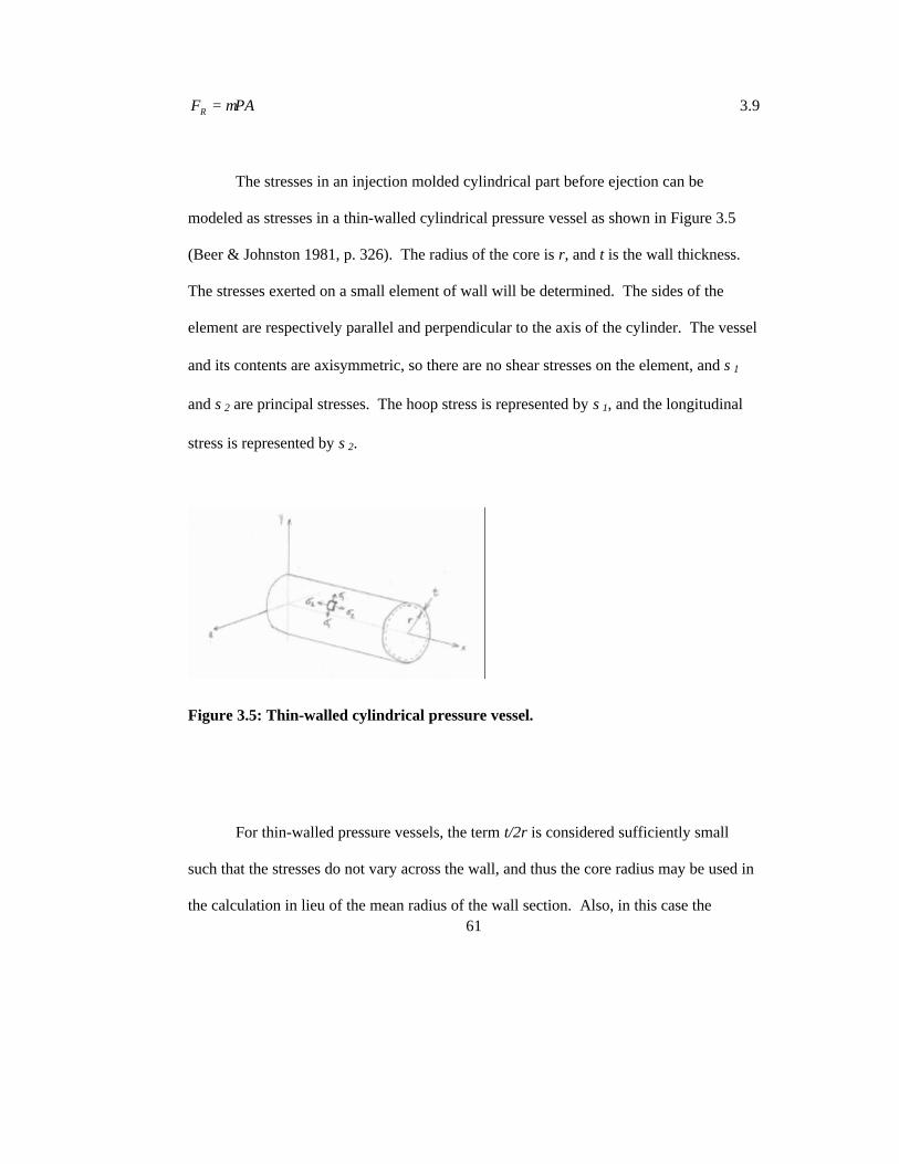
61

PAFR µ= 3.9

The stresses in an injection molded cylindrical part before ejection can be

modeled as stresses in a thin-walled cylindrical pressure vessel as shown in Figure 3.5

(Beer & Johnston 1981, p. 326). The radius of the core is r, and t is the wall thickness.

The stresses exerted on a small element of wall will be determined. The sides of the

element are respectively parallel and perpendicular to the axis of the cylinder. The vessel

and its contents are axisymmetric, so there are no shear stresses on the element, and σ1

and σ2 are principal stresses. The hoop stress is represented by σ1, and the longitudinal

stress is represented by σ2.

Figure 3.5: Thin-walled cylindrical pressure vessel.

For thin-walled pressure vessels, the term t/2r is considered sufficiently small

such that the stresses do not vary across the wall, and thus the core radius may be used in

the calculation in lieu of the mean radius of the wall section. Also, in this case the

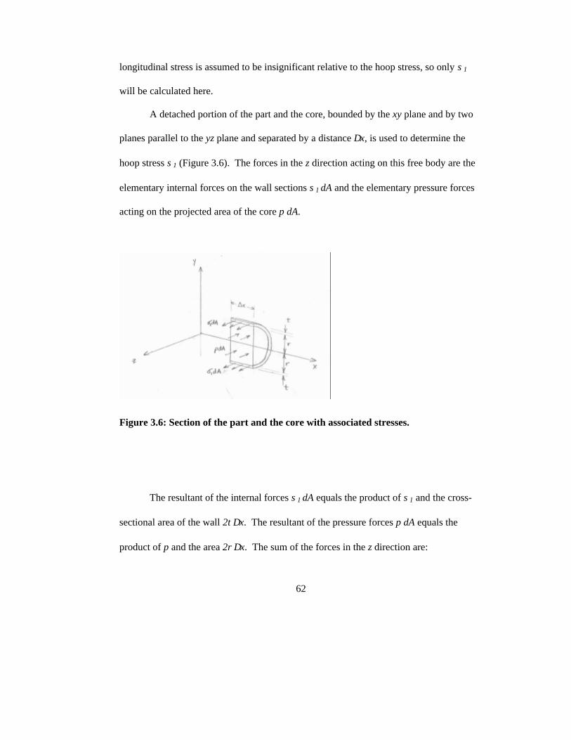
62

longitudinal stress is assumed to be insignificant relative to the hoop stress, so only σ1

will be calculated here.

A detached portion of the part and the core, bounded by the xy plane and by two

planes parallel to the yz plane and separated by a distance ∆x, is used to determine the

hoop stress σ1 (Figure 3.6). The forces in the z direction acting on this free body are the

elementary internal forces on the wall sections σ1 dA and the elementary pressure forces

acting on the projected area of the core p dA.

Figure 3.6: Section of the part and the core with associated stresses.

The resultant of the internal forces σ1 dA equals the product of σ1 and the cross-

sectional area of the wall 2t ∆x. The resultant of the pressure forces p dA equals the

product of p and the area 2r ∆x. The sum of the forces in the z direction are:

63

:0=Σ zF ( ) ( ) 0221 =∆−∆ xrpxtσ 3.10

Solving for hoop stress σ1:

tpr

=1σ 3.11

Rearranging equation 3.11 to solve for the pressure force, i.e., the contact pressure P in

this case:

crt

Pσ

= 3.12

Next, Hooke’s Law is applied, assuming elasticity in the solidified part.

According to equation 3.12, contact pressure P is proportional to tensile (circumferential)

stress σ. Stress σ is directly proportional to the elastic modulus and strain Eε:

( )εσ TE= 3.13

where E(T) is the elastic modulus at the ejection temperature, and ε represents

engineering strain. The injection molding case involves changing temperatures, thus

strain can be represented by thermal strain as follows:

64

( )EM TT −= αε 3.14

where α is the coefficient of thermal expansion, TM is the melt temperature, and TE is the

temperature at ejection. Combining equations 3.13 and 3.14 gives:

( ) ( )EM TTTE −= ασ 3.15

As previously mentioned, the term t/2r must be sufficiently small in order to

apply the equation for thin-walled pressure vessels. For example, ensuring that 102 crt < is

a good rule of thumb (Popov 1976, p 290). Combining equations 3.12 and 3.15 gives:

( )c

EM

rtTTTE

P−

=α)(

3.16

With the area of the cylinder LDA cπ= and equations 3.9 and 3.16:

( ) ( )c

cEMR r

LDtTTTEF

παµ −= 3.17

Menges et al (2001) approximate strain by the relative change in diameter ∆dr of

the cylinder immediately after ejection. With this change, then, the ejection force is:

65

( )c

crR r

LDtdTEF

πµ ∆= 3.18

3.3.2 Additional Consideration for Strain

The description of strain in equation 3.14 may be a simplification considering

other transformations within the material. For example, in addition to thermal strain,

there may also be crystallization strain for crystalline materials, reaction strain for

thermosets, and hydrostatic strain due to the compressibility of the material (Jansen &

Titomanlio 1996). Total strain would be the sum of thermal strain, hydrostatic strain, and

crystallization and reaction strain as applicable. In this work, reaction strain does not

apply, and crystallization strain would only apply to HDPE, since HIPS is amorphous.

By using a measure of relative change in diameter in place of thermal strain, as shown in

equation 3.18, all aspects of strain are taken into consideration. Thus ∆dr represents total

strain, and improves the accuracy of the ejection force model.

66

CHAPTER 4

EXPERIMENTATION

This chapter describes the details about how data were collected for this research.

For friction testing, this includes a description of the test apparatus and the test matrix

and procedure. The process for measurement of thermoplastic modulus at temperature is

then presented. For the injection molding experiments, the mold and part design, the

injection molding machine and process parameters, and the experimental design and

procedure are all explained. The last section on data acquisition summarizes core

temperature, ejection force, and part diameter measurements.

4.1 Friction Testing

Most published data on coefficients of friction for thermoplastics result from

room temperature tests against steel or against like materials. For example, the ASM

Handbook lists friction data for polymers on steel as shown in Table 4.1 (ASM

International 1992). Actual friction coefficients during the injection molding process are

difficult to determine because of the rapidly changing temperature and pressure

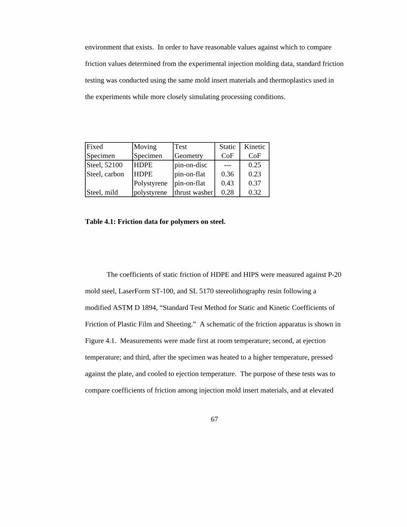
67

environment that exists. In order to have reasonable values against which to compare

friction values determined from the experimental injection molding data, standard friction

testing was conducted using the same mold insert materials and thermoplastics used in

the experiments while more closely simulating processing conditions.

Table 4.1: Friction data for polymers on steel.

The coefficients of static friction of HDPE and HIPS were measured against P-20

mold steel, LaserForm ST-100, and SL 5170 stereolithography resin following a

modified ASTM D 1894, “Standard Test Method for Static and Kinetic Coefficients of

Friction of Plastic Film and Sheeting.” A schematic of the friction apparatus is shown in

Figure 4.1. Measurements were made first at room temperature; second, at ejection

temperature; and third, after the specimen was heated to a higher temperature, pressed

against the plate, and cooled to ejection temperature. The purpose of these tests was to

compare coefficients of friction among injection mold insert materials, and at elevated

Fixed Specimen

Moving Specimen

Test Geometry

Static CoF

Kinetic CoF

Steel, 52100 HDPE pin-on-disc --- 0.25Steel, carbon HDPE pin-on-flat 0.36 0.23

Polystyrene pin-on-flat 0.43 0.37Steel, mild polystyrene thrust washer 0.28 0.32

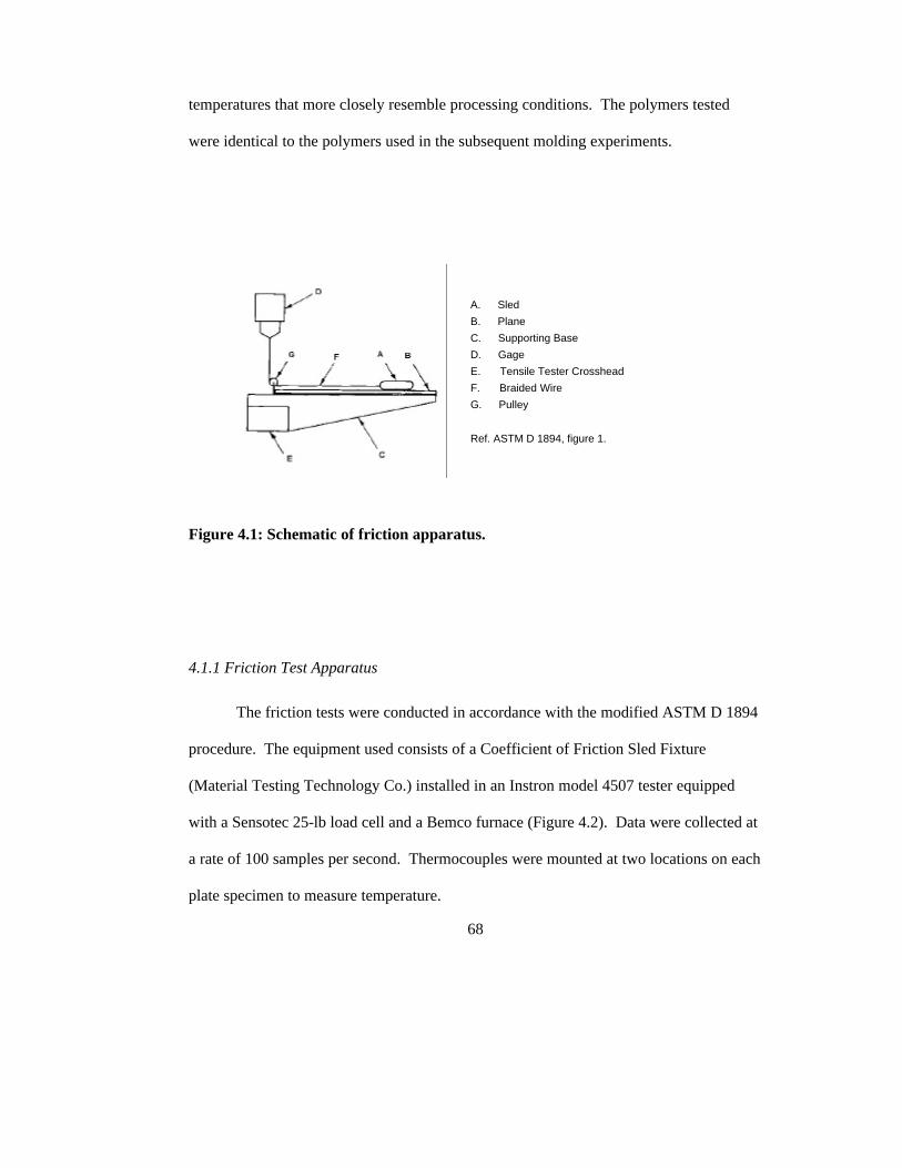
68

temperatures that more closely resemble processing conditions. The polymers tested

were identical to the polymers used in the subsequent molding experiments.

Figure 4.1: Schematic of friction apparatus.

4.1.1 Friction Test Apparatus

The friction tests were conducted in accordance with the modified ASTM D 1894

procedure. The equipment used consists of a Coefficient of Friction Sled Fixture

(Material Testing Technology Co.) installed in an Instron model 4507 tester equipped

with a Sensotec 25-lb load cell and a Bemco furnace (Figure 4.2). Data were collected at

a rate of 100 samples per second. Thermocouples were mounted at two locations on each

plate specimen to measure temperature.

A.       Sled

B.       Plane

C.       Supporting Base

D.       Gage

E.        Tensile Tester Crosshead

F.        Braided Wire

G.       Pulley

Ref. ASTM D 1894, figure 1.

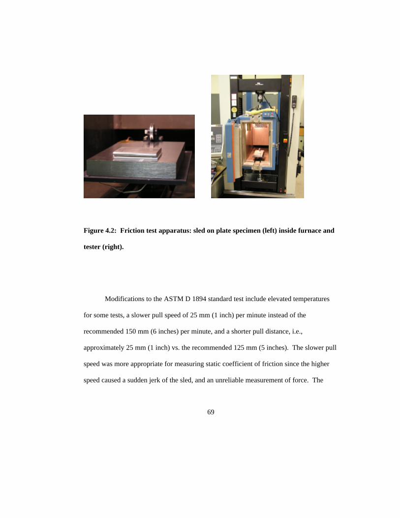
69

Figure 4.2: Friction test apparatus: sled on plate specimen (left) inside furnace and

tester (right).

Modifications to the ASTM D 1894 standard test include elevated temperatures

for some tests, a slower pull speed of 25 mm (1 inch) per minute instead of the

recommended 150 mm (6 inches) per minute, and a shorter pull distance, i.e.,

approximately 25 mm (1 inch) vs. the recommended 125 mm (5 inches). The slower pull

speed was more appropriate for measuring static coefficient of friction since the higher

speed caused a sudden jerk of the sled, and an unreliable measurement of force. The

70

shorter pull distance was used because, for determining static friction, only the force

necessary to set the sled in motion is required.

4.1.2 Test Matrix and Procedure

The friction test matrix is shown in Table 4.2. Two thermoplastics and three mold

insert materials were tested under three temperature conditions. The thermoplastic

specimens were 63.5 mm (2.5 inches) square and attached to the sled using double-sided,

high temperature fiberglass tape. The mold insert material specimens were

approximately 125 mm (5 inches) wide by 250 mm (10 inches) long and were positioned

on the base plate of the apparatus. The surface roughnesses of the plate specimens were

0.7 microns (28 microinches) for P-20, 0.2 microns (8 microinches) for ST-100, and 3.6

microns (142 microinches) for SL 5170.

The first temperature condition was room temperature, 22 oC (71 oF). The second

condition was ejection temperature, i.e., the temperature at which molded parts are

ejected from the injection molding machine. The second temperature condition simulated

the environment in which friction is encountered in the injection molding process, i.e., 50

oC (120 oF) for P-20 and ST-100 plate materials and 55 oC (130 oF) for SL 5170 plate

material. The third condition consisted of first heating to an elevated temperature (120

oC (250 oF) for HDPE specimens and 150 oC (300 oF) for HIPS specimens), then cooling

down to the ejection temperatures mentioned above before testing. While at the elevated

temperature, a 0.9 kg (2-lb) mass was placed on the sled. When the plate cooled to

ejection temperature, the weight was removed and the specimen tested. The purpose of

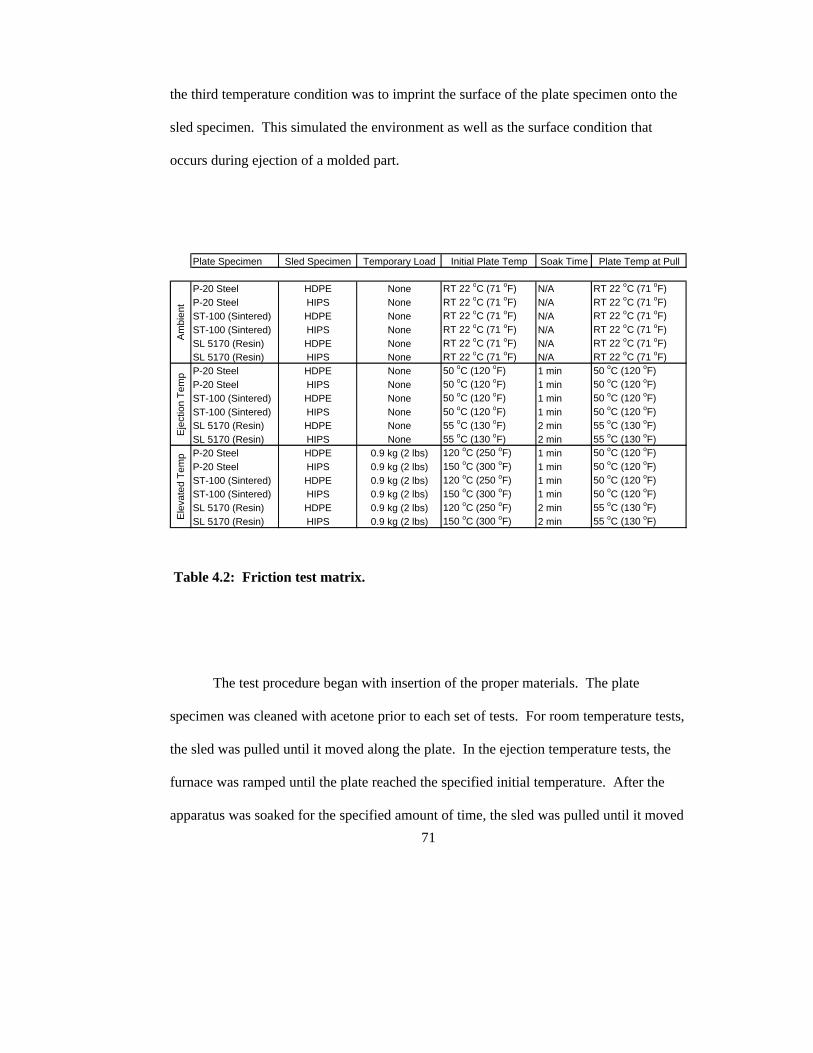
71

the third temperature condition was to imprint the surface of the plate specimen onto the

sled specimen. This simulated the environment as well as the surface condition that

occurs during ejection of a molded part.

Table 4.2: Friction test matrix.

The test procedure began with insertion of the proper materials. The plate

specimen was cleaned with acetone prior to each set of tests. For room temperature tests,

the sled was pulled until it moved along the plate. In the ejection temperature tests, the

furnace was ramped until the plate reached the specified initial temperature. After the

apparatus was soaked for the specified amount of time, the sled was pulled until it moved

Plate Specimen Sled Specimen Temporary Load Initial Plate Temp Soak Time Plate Temp at Pull

P-20 Steel HDPE None RT 22 oC (71 oF) N/A RT 22 oC (71 oF)P-20 Steel HIPS None RT 22 oC (71 oF) N/A RT 22 oC (71 oF)ST-100 (Sintered) HDPE None RT 22 oC (71 oF) N/A RT 22 oC (71 oF)ST-100 (Sintered) HIPS None RT 22 oC (71 oF) N/A RT 22 oC (71 oF)SL 5170 (Resin) HDPE None RT 22 oC (71 oF) N/A RT 22 oC (71 oF)SL 5170 (Resin) HIPS None RT 22 oC (71 oF) N/A RT 22 oC (71 oF)P-20 Steel HDPE None 50 oC (120 oF) 1 min 50 oC (120 oF)P-20 Steel HIPS None 50 oC (120 oF) 1 min 50 oC (120 oF)ST-100 (Sintered) HDPE None 50 oC (120 oF) 1 min 50 oC (120 oF)ST-100 (Sintered) HIPS None 50 oC (120 oF) 1 min 50 oC (120 oF)SL 5170 (Resin) HDPE None 55 oC (130 oF) 2 min 55 oC (130 oF)SL 5170 (Resin) HIPS None 55 oC (130 oF) 2 min 55 oC (130 oF)P-20 Steel HDPE 0.9 kg (2 lbs) 120 oC (250 oF) 1 min 50 oC (120 oF)P-20 Steel HIPS 0.9 kg (2 lbs) 150 oC (300 oF) 1 min 50 oC (120 oF)ST-100 (Sintered) HDPE 0.9 kg (2 lbs) 120 oC (250 oF) 1 min 50 oC (120 oF)ST-100 (Sintered) HIPS 0.9 kg (2 lbs) 150 oC (300 oF) 1 min 50 oC (120 oF)SL 5170 (Resin) HDPE 0.9 kg (2 lbs) 120 oC (250 oF) 2 min 55 oC (130 oF)SL 5170 (Resin) HIPS 0.9 kg (2 lbs) 150 oC (300 oF) 2 min 55 oC (130 oF)

Am

bien

tE

ject

ion

Tem

pE

leva

ted

Tem

p

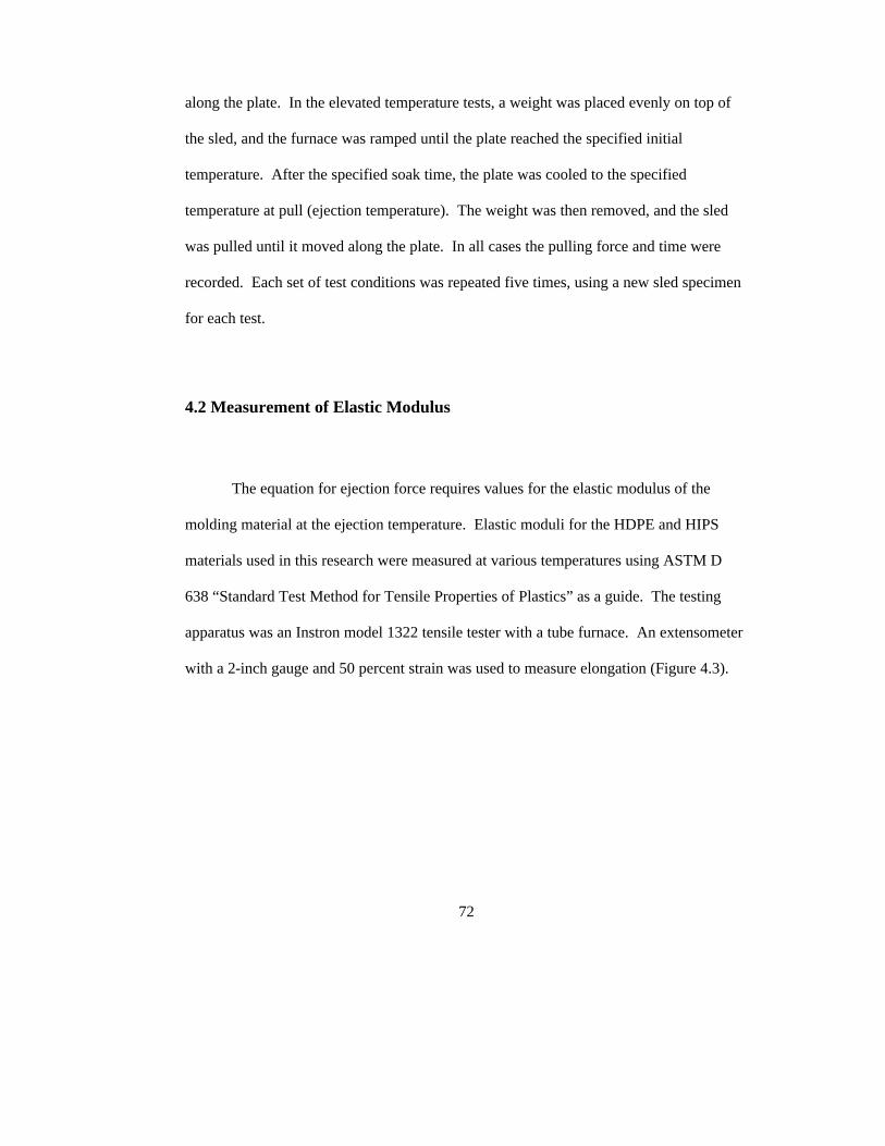
72

along the plate. In the elevated temperature tests, a weight was placed evenly on top of

the sled, and the furnace was ramped until the plate reached the specified initial

temperature. After the specified soak time, the plate was cooled to the specified

temperature at pull (ejection temperature). The weight was then removed, and the sled

was pulled until it moved along the plate. In all cases the pulling force and time were

recorded. Each set of test conditions was repeated five times, using a new sled specimen

for each test.

4.2 Measurement of Elastic Modulus

The equation for ejection force requires values for the elastic modulus of the

molding material at the ejection temperature. Elastic moduli for the HDPE and HIPS

materials used in this research were measured at various temperatures using ASTM D

638 “Standard Test Method for Tensile Properties of Plastics” as a guide. The testing

apparatus was an Instron model 1322 tensile tester with a tube furnace. An extensometer

with a 2-inch gauge and 50 percent strain was used to measure elongation (Figure 4.3).

73

Figure 4.3: Tensile testing apparatus with tube furnace.

ASTM Type I (dogbone) specimens were molded from each thermoplastic

material and were tested at room temperature, 30oC, and at ten degree increments until no

elastic region was detected (Figure 4.4). HDPE was tested through 70oC, and HIPS was

tested through 50oC. At least three samples of HIPS were tested at each temperature,

while at least 5 samples of HDPE were tested at each temperature. Data from the tensile

tests are included in Appendix A, and a graph of the results is shown in Figure 4.5.

Modulus values for HIPS at higher ejection temperatures than 50oC were determined by

extrapolating the graph. The lookup table generated from this graph and used in the

calculations of friction coefficient can also be found in Appendix A.

74

Figure 4.4: HIPS specimens after tensile tests.

Figure 4.5: Elastic modulus at various temperatures for HDPE and HIPS.

0

500

1000

1500

2000

2500

3000

3500

4000

20 30 40 50 60 70 80

Temperature (°C)

Mo

du

lus

(MP

a)

HIPS PS 495F

HDPE ME 9180

75

4.3 Injection Molding

4.3.1 Mold Design and Materials

Since this research involved the study of different rapid tooling materials, a

modular mold design was employed. The mold base was a steel Master Unit Die (MUD)

having a core and cavity that could be removed and replaced with those of other materials

(Figure 4.6). The baseline core and cavity were made of P-20 steel, a typical mold steel,

and the two rapid tooled core and cavity sets were made of SL 5170 epoxy resin and

LaserForm ST-100 material (Figure 4.7). The SL 5170 insert was built at NASA

Marshall Space Flight Center using the stereolithography process, and the ST-100 insert

was built at General Pattern Company (Blaine, MN) using the laser sintering process, as

described in Chapter 2. Machining allowances were included in the design of each rapid

tooled insert so that it could be machined to fit properly into the mold base. The baseline

steel insert core had a surface finish of Ra = 0.7 microns (28 microinches). The

stereolithography insert also had a surface finish of Ra = 0.7 microns (28 microinches),

and the laser sintered insert had a surface finish of Ra = 0.3 microns (12 microinches).

76

Figure 4.6: Sprue side of the MUD base mounted in the injection molding machine

with SL 5170 cavity insert.

Figure 4.7: Core and cavity inserts, before final machining, made of SL 5170 (left),

P-20 steel (center), and LaserForm ST-100 (right).

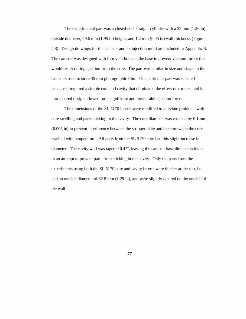
77

The experimental part was a closed-end, straight cylinder with a 32 mm (1.26 in)

outside diameter, 49.6 mm (1.95 in) height, and 1.2 mm (0.05 in) wall thickness (Figure

4.8). Design drawings for the canister and its injection mold are included in Appendix B.

The canister was designed with four vent holes in the base to prevent vacuum forces that

would result during ejection from the core. The part was similar in size and shape to the

canisters used to store 35 mm photographic film. This particular part was selected

because it required a simple core and cavity that eliminated the effect of corners, and its

non-tapered design allowed for a significant and measurable ejection force.

The dimensions of the SL 5170 inserts were modified to alleviate problems with

core swelling and parts sticking in the cavity. The core diameter was reduced by 0.1 mm,

(0.005 in) to prevent interference between the stripper plate and the core when the core

swelled with temperature. All parts from the SL 5170 core had this slight increase in

diameter. The cavity wall was tapered 0.42o, leaving the canister base dimension intact,

in an attempt to prevent parts from sticking in the cavity. Only the parts from the

experiments using both the SL 5170 core and cavity inserts were thicker at the rim, i.e.,

had an outside diameter of 32.8 mm (1.29 in), and were slightly tapered on the outside of

the wall.

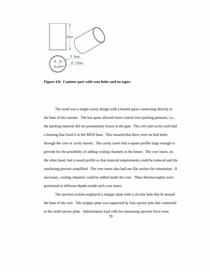
78

Figure 4.8: Canister part with vent holes and no taper.

The mold was a single-cavity design with a heated sprue connecting directly to

the base of the canister. The hot sprue allowed more control over packing pressure, i.e.,

the packing material did not prematurely freeze at the gate. The core and cavity each had

a housing that fixed it to the MUD base. This ensured that there were no bolt holes

through the core or cavity inserts. The cavity insert had a square profile large enough to

provide for the possibility of adding cooling channels in the future. The core insert, on

the other hand, had a round profile so that material requirements could be reduced and the

machining process simplified. The core insert also had one flat surface for orientation. If

necessary, cooling channels could be added inside the core. Three thermocouples were

positioned at different depths inside each core insert.

The ejection system employed a stripper plate with a circular hole that fit around

the base of the core. The stripper plate was supported by four ejector pins that connected

to the mold ejector plate. Subminiature load cells for measuring ejection force were

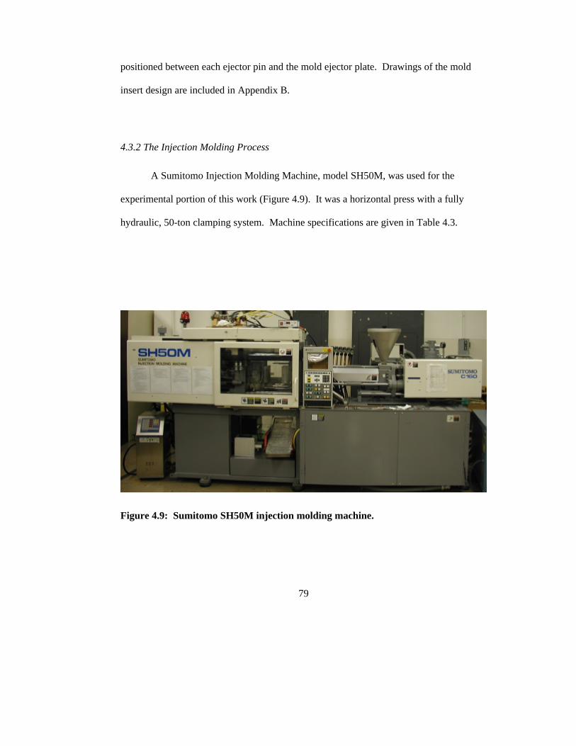
79

positioned between each ejector pin and the mold ejector plate. Drawings of the mold

insert design are included in Appendix B.

4.3.2 The Injection Molding Process

A Sumitomo Injection Molding Machine, model SH50M, was used for the

experimental portion of this work (Figure 4.9). It was a horizontal press with a fully

hydraulic, 50-ton clamping system. Machine specifications are given in Table 4.3.

Figure 4.9: Sumitomo SH50M injection molding machine.

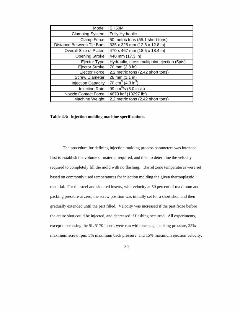
80

Table 4.3: Injection molding machine specifications.

The procedure for defining injection molding process parameters was intended

first to establish the volume of material required, and then to determine the velocity

required to completely fill the mold with no flashing. Barrel zone temperatures were set

based on commonly used temperatures for injection molding the given thermoplastic

material. For the steel and sintered inserts, with velocity at 50 percent of maximum and

packing pressure at zero, the screw position was initially set for a short shot, and then

gradually extended until the part filled. Velocity was increased if the part froze before

the entire shot could be injected, and decreased if flashing occurred. All experiments,

except those using the SL 5170 insert, were run with one stage packing pressure, 25%

maximum screw rpm, 5% maximum back pressure, and 15% maximum ejection velocity.

Model SH50MClamping System Fully Hydraulic

Clamp Force 50 metric tons (55.1 short tons)Distance Between Tie Bars 325 x 325 mm (12.8 x 12.8 in)

Overall Size of Platen 470 x 467 mm (18.5 x 18.4 in)Opening Stroke 440 mm (17.3 in)

Ejector Type Hydraulic, cross multipoint ejection (5pts)Ejector Stroke 70 mm (2.8 in)Ejector Force 2.2 metric tons (2.42 short tons)

Screw Diameter 28 mm (1.1 in)Injection Capacity 70 cm3 (4.3 in3)

Injection Rate 99 cm3/s (6.0 in3/s)Nozzle Contact Force 4670 kgf (10297 lbf)

Machine Weight 2.2 metric tons (2.42 short tons)

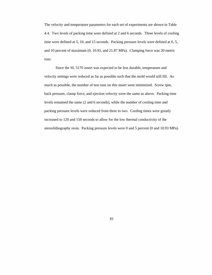
81

The velocity and temperature parameters for each set of experiments are shown in Table

4.4. Two levels of packing time were defined at 2 and 6 seconds. Three levels of cooling

time were defined at 5, 10, and 15 seconds. Packing pressure levels were defined at 0, 5,

and 10 percent of maximum (0, 10.93, and 21.87 MPa). Clamping force was 20 metric

tons.

Since the SL 5170 insert was expected to be less durable, temperature and

velocity settings were reduced as far as possible such that the mold would still fill. As

much as possible, the number of test runs on this insert were minimized. Screw rpm,

back pressure, clamp force, and ejection velocity were the same as above. Packing time

levels remained the same (2 and 6 seconds), while the number of cooling time and

packing pressure levels were reduced from three to two. Cooling times were greatly

increased to 120 and 150 seconds to allow for the low thermal conductivity of the

stereolithography resin. Packing pressure levels were 0 and 5 percent (0 and 10.93 MPa).

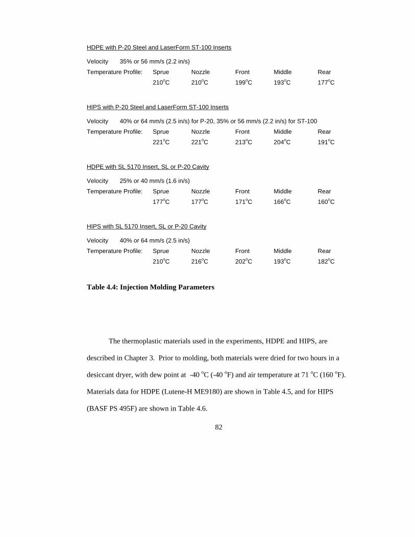
82

HDPE with P-20 Steel and LaserForm ST-100 Inserts

Velocity 35% or 56 mm/s (2.2 in/s)

Temperature Profile: Sprue Nozzle Front Middle Rear

210oC 210oC 199oC 193oC 177oC

HIPS with P-20 Steel and LaserForm ST-100 Inserts

Velocity 40% or 64 mm/s (2.5 in/s) for P-20, 35% or 56 mm/s (2.2 in/s) for ST-100

Temperature Profile: Sprue Nozzle Front Middle Rear

221oC 221oC 213oC 204oC 191oC

HDPE with SL 5170 Insert, SL or P-20 Cavity

Velocity 25% or 40 mm/s (1.6 in/s)

Temperature Profile: Sprue Nozzle Front Middle Rear

177oC 177oC 171oC 166oC 160oC

HIPS with SL 5170 Insert, SL or P-20 Cavity

Velocity 40% or 64 mm/s (2.5 in/s)

Temperature Profile: Sprue Nozzle Front Middle Rear

210oC 216oC 202oC 193oC 182oC

Table 4.4: Injection Molding Parameters

The thermoplastic materials used in the experiments, HDPE and HIPS, are

described in Chapter 3. Prior to molding, both materials were dried for two hours in a

desiccant dryer, with dew point at -40 oC (-40 oF) and air temperature at 71 oC (160 oF).

Materials data for HDPE (Lutene-H ME9180) are shown in Table 4.5, and for HIPS

(BASF PS 495F) are shown in Table 4.6.

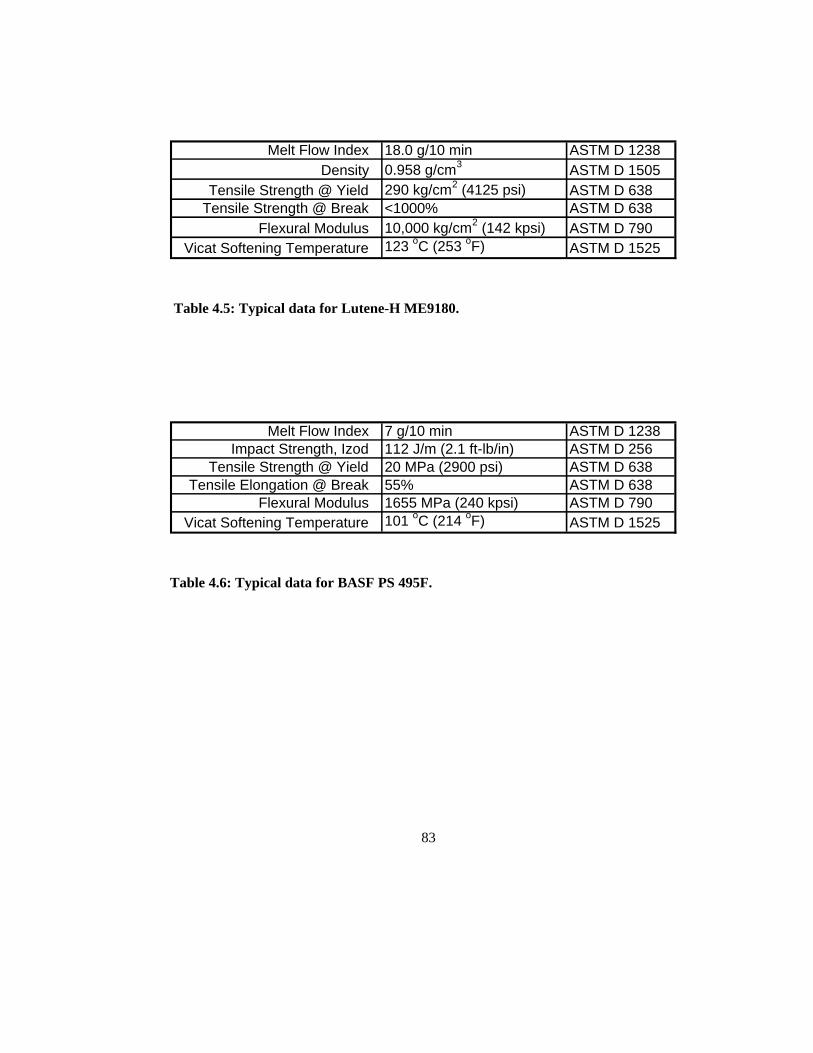
83

Table 4.5: Typical data for Lutene-H ME9180.

Table 4.6: Typical data for BASF PS 495F.

Melt Flow Index 18.0 g/10 min ASTM D 1238Density 0.958 g/cm3 ASTM D 1505

Tensile Strength @ Yield 290 kg/cm2 (4125 psi) ASTM D 638Tensile Strength @ Break <1000% ASTM D 638

Flexural Modulus 10,000 kg/cm2 (142 kpsi) ASTM D 790Vicat Softening Temperature 123 oC (253 oF) ASTM D 1525

Melt Flow Index 7 g/10 min ASTM D 1238Impact Strength, Izod 112 J/m (2.1 ft-lb/in) ASTM D 256

Tensile Strength @ Yield 20 MPa (2900 psi) ASTM D 638Tensile Elongation @ Break 55% ASTM D 638

Flexural Modulus 1655 MPa (240 kpsi) ASTM D 790Vicat Softening Temperature 101 oC (214 oF) ASTM D 1525

84

4.3.3 Design of Experiments

Statistical design of experiments has been used to design the six sets of

experiments run in this work. Each set was blocked by insert material and thermoplastic

material, and then randomized by packing time, cooling time and packing pressure. In

the first four experimental sets, there were two levels of packing time, three levels of

cooling time, and three levels of packing pressure as described above. Each combination

of factors was repeated eight times. The experimental design with process parameters is

shown in Table 4.7.

The last two experimental sets, using the SL 5170 insert, were designed to be

smaller than the other sets due to the expected low durability of the insert material. In

this case there were two levels each of packing time, cooling time, and packing pressure

as described above. Each combination of factors was repeated five times. A much

longer cooling time was required for this insert to accommodate its low thermal

conductivity. It was initially intended that cooling time levels be set at 150 and 180

seconds. However these levels were reduced to 120 and 150 seconds to reduce the

shrinkage on the core, and thus ejection force requirements. Also note that only a limited

number of parts could be processed using the SL 5170 cavities due to deformation that

caused sticking of parts (see Chapter 6). The designed experiment, therefore, was carried

out using the SL 5170 core with the P-20 cavity. While the use of steel cavity material

greatly changed the thermal performance of this insert and reduced the temperature at

ejection, it also allowed a complete experiment to be performed in which ejection force

from the SL 5170 core could be measured.

85

Design of experiments (DOE) analyses in Minitab® have been performed using

packing time, cooling time and packing pressure as factors and ejection force as the

response. Using analysis of variance (ANOVA), the effects of variables and their

interactions on each response were determined. ANOVA tables for each data set are

included in Appendix A. DOE results and graphs identifying main effects and

interactions are included in Chapter 5.

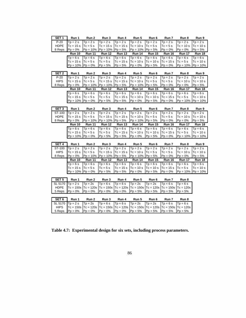
86

Table 4.7: Experimental design for six sets, including process parameters.

SET 1 Run 1 Run 2 Run 3 Run 4 Run 5 Run 6 Run 7 Run 8 Run 9P-20 Tp = 2 s Tp = 2 s Tp = 2 s Tp = 2 s Tp = 2 s Tp = 2 s Tp = 2 s Tp = 2 s Tp = 2 s

HDPE Tc = 15 s Tc = 5 s Tc = 15 s Tc = 15 s Tc = 10 s Tc = 5 s Tc = 5 s Tc = 10 s Tc = 10 s8 Reps Pp = 0% Pp = 10% Pp = 10% Pp = 5% Pp = 10% Pp = 5% Pp = 0% Pp = 0% Pp = 5%

Run 10 Run 11 Run 12 Run 13 Run 14 Run 15 Run 16 Run 17 Run 18Tp = 6 s Tp = 6 s Tp = 6 s Tp = 6 s Tp = 6 s Tp = 6 s Tp = 6 s Tp = 6 s Tp = 6 sTc = 15 s Tc = 5 s Tc = 5 s Tc = 15 s Tc = 10 s Tc = 10 s Tc = 15 s Tc = 5 s Tc = 10 sPp = 10% Pp = 0% Pp = 5% Pp = 5% Pp = 0% Pp = 5% Pp = 0% Pp = 10% Pp = 10%

SET 2 Run 1 Run 2 Run 3 Run 4 Run 5 Run 6 Run 7 Run 8 Run 9P-20 Tp = 2 s Tp = 2 s Tp = 2 s Tp = 2 s Tp = 2 s Tp = 2 s Tp = 2 s Tp = 2 s Tp = 2 sHIPS Tc = 15 s Tc = 5 s Tc = 15 s Tc = 15 s Tc = 10 s Tc = 5 s Tc = 5 s Tc = 10 s Tc = 10 s

8 Reps Pp = 0% Pp = 10% Pp = 10% Pp = 5% Pp = 10% Pp = 5% Pp = 0% Pp = 0% Pp = 5%Run 10 Run 11 Run 12 Run 13 Run 14 Run 15 Run 16 Run 17 Run 18

Tp = 6 s Tp = 6 s Tp = 6 s Tp = 6 s Tp = 6 s Tp = 6 s Tp = 6 s Tp = 6 s Tp = 6 sTc = 15 s Tc = 5 s Tc = 5 s Tc = 15 s Tc = 10 s Tc = 10 s Tc = 15 s Tc = 5 s Tc = 10 sPp = 10% Pp = 0% Pp = 5% Pp = 5% Pp = 0% Pp = 5% Pp = 0% Pp = 10% Pp = 10%

SET 3 Run 1 Run 2 Run 3 Run 4 Run 5 Run 6 Run 7 Run 8 Run 9ST-100 Tp = 2 s Tp = 2 s Tp = 2 s Tp = 2 s Tp = 2 s Tp = 2 s Tp = 2 s Tp = 2 s Tp = 2 sHDPE Tc = 15 s Tc = 5 s Tc = 15 s Tc = 15 s Tc = 10 s Tc = 5 s Tc = 5 s Tc = 10 s Tc = 10 s8 Reps Pp = 0% Pp = 10% Pp = 10% Pp = 5% Pp = 10% Pp = 5% Pp = 0% Pp = 0% Pp = 5%

Run 10 Run 11 Run 12 Run 13 Run 14 Run 15 Run 16 Run 17 Run 18Tp = 6 s Tp = 6 s Tp = 6 s Tp = 6 s Tp = 6 s Tp = 6 s Tp = 6 s Tp = 6 s Tp = 6 sTc = 15 s Tc = 5 s Tc = 5 s Tc = 15 s Tc = 10 s Tc = 10 s Tc = 15 s Tc = 5 s Tc = 10 sPp = 10% Pp = 0% Pp = 5% Pp = 5% Pp = 0% Pp = 5% Pp = 0% Pp = 10% Pp = 10%

SET 4 Run 1 Run 2 Run 3 Run 4 Run 5 Run 6 Run 7 Run 8 Run 9ST-100 Tp = 2 s Tp = 2 s Tp = 2 s Tp = 2 s Tp = 2 s Tp = 2 s Tp = 2 s Tp = 2 s Tp = 2 sHIPS Tc = 15 s Tc = 5 s Tc = 15 s Tc = 15 s Tc = 10 s Tc = 5 s Tc = 5 s Tc = 10 s Tc = 10 s

8 Reps Pp = 0% Pp = 10% Pp = 10% Pp = 5% Pp = 10% Pp = 5% Pp = 0% Pp = 0% Pp = 5%Run 10 Run 11 Run 12 Run 13 Run 14 Run 15 Run 16 Run 17 Run 18

Tp = 6 s Tp = 6 s Tp = 6 s Tp = 6 s Tp = 6 s Tp = 6 s Tp = 6 s Tp = 6 s Tp = 6 sTc = 15 s Tc = 5 s Tc = 5 s Tc = 15 s Tc = 10 s Tc = 10 s Tc = 15 s Tc = 5 s Tc = 10 sPp = 10% Pp = 0% Pp = 5% Pp = 5% Pp = 0% Pp = 5% Pp = 0% Pp = 10% Pp = 10%

SET 5 Run 1 Run 2 Run 3 Run 4 Run 5 Run 6 Run 7 Run 8SL 5170 Tp = 2 s Tp = 2s Tp = 6 s Tp = 6 s Tp = 2s Tp = 2s Tp = 6 s Tp = 6 sHDPE Tc = 150s Tc = 120s Tc = 150s Tc = 120s Tc = 150s Tc = 120s Tc = 150s Tc = 120s5 Reps Pp = 0% Pp = 0% Pp = 0% Pp = 0% Pp = 5% Pp = 5% Pp = 5% Pp = 5%

SET 6 Run 1 Run 2 Run 3 Run 4 Run 5 Run 6 Run 7 Run 8SL 5170 Tp = 2 s Tp = 2s Tp = 6 s Tp = 6 s Tp = 2s Tp = 2s Tp = 6 s Tp = 6 s

HIPS Tc = 150s Tc = 120s Tc = 150s Tc = 120s Tc = 150s Tc = 120s Tc = 150s Tc = 120s5 Reps Pp = 0% Pp = 0% Pp = 0% Pp = 0% Pp = 5% Pp = 5% Pp = 5% Pp = 5%

87

4.3.4 Experimental Procedure

An experimental set was defined by the mold insert and thermoplastic material.

The procedure followed for each experimental set is as follows:

1) Begin Set

2) Setup hardware and load thermoplastic material

3) Load parameter settings

4) Begin Run

i) Adjust DOE settings for packing time, cooling time and packing pressure

ii) Process test parts to bring insert to temperature

iii) Begin Iteration

(a) Inject part

(b) Capture ejection force and temperature during ejection

(c) Digitally photograph part immediately after ejection

(d) Wait for core to return to desired temperature

iv) Repeat iteration 8 times (5 times with SL 5170 insert)

5) Repeat run for all DOE combinations

6) Go to next set

Ejection force data were used to determine the initial force required to release

each part from the core. Thermal data were used to determine the elastic modulus of

each thermoplastic at ejection. Inside and outside diameters of the canister parts,

88

measured from digital photographs, were used to determine part thickness. All of these

data were used with the Menges ejection force model to calculate the ejection force and

the apparent coefficient of static friction. Statistical analysis of variance, as described

above, was conducted using packing time, cooling time, and packing pressure as input

factors, and ejection force as the response. Experimental results and conclusions are

included in Chapters 5 and 6. Experimental data are included in Appendix A.

4.4 Set-up and Data Acquisition

The data required from the injection molding experiments included thermal (core

temperature at ejection), load (ejection force), and dimensional (part diameter and

thickness at ejection) measurements. Type J thermocouples were used to measure

temperature, subminiature load cells were used to measure force, and digital imaging was

used to measure diameter. The three thermal and four load sensors collected data through

a National Instruments SC-2311 signal conditioner with associated thermocouple and

strain gage input modules. A LabVIEW™ program was used to read the ejection force

and temperature data and write them to a Microsoft Excel® spreadsheet. Pictures of each

part were taken with an Olympus Camedia C-740 digital camera and processed using

Adobe PhotoShop software. The inside and outside diameters of each part were

measured in pixels and converted to inches and millimeters by reference to a scale, a

picture of which was taken during each set of experiments. The data acquisition

equipment is shown in Figure 4.10.

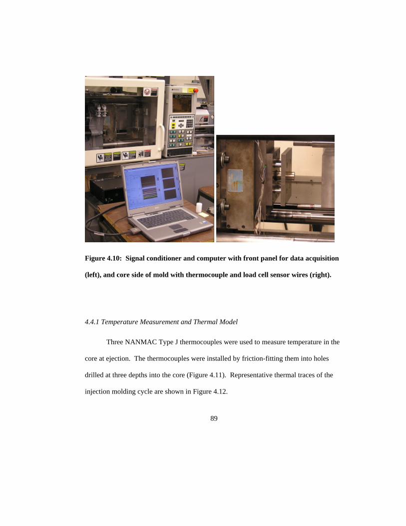
89

Figure 4.10: Signal conditioner and computer with front panel for data acquisition

(left), and core side of mold with thermocouple and load cell sensor wires (right).

4.4.1 Temperature Measurement and Thermal Model

Three NANMAC Type J thermocouples were used to measure temperature in the

core at ejection. The thermocouples were installed by friction-fitting them into holes

drilled at three depths into the core (Figure 4.11). Representative thermal traces of the

injection molding cycle are shown in Figure 4.12.

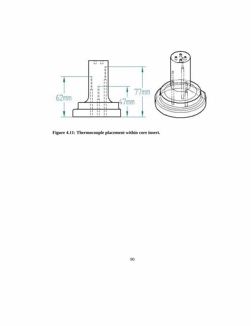
90

Figure 4.11: Thermocouple placement within core insert.

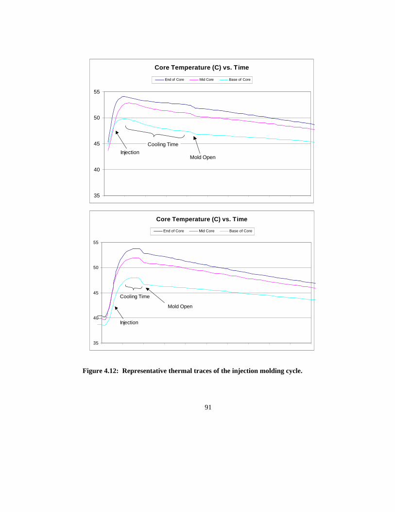
91

Figure 4.12: Representative thermal traces of the injection molding cycle.

Core Temperature (C) vs. Time

35

40

45

50

55

End of Core Mid Core Base of Core

InjectionCooling Time

Mold Open

Core Temperature (C) vs. Time

35

40

45

50

55

End of Core Mid Core Base of Core

Injection

Cooling Time

Mold Open

92

Since the distance between each thermocouple and the surface of the core was

more than a millimeter, there was a time lag from heating of the surface to heating of the

thermocouple. A thermal analysis was run to determine the convergence time between

the thermocouple reading and the actual temperature at the surface of the core (Carpenter

2004). The analysis simulated injection of the thermoplastic into the mold insert for each

material combination. The simulation was run using ABAQUS, and the results show the

time required for temperature at the thermocouple to match the temperature at the surface

of the core (Table 4.8). Initial and boundary conditions for the thermal analysis are

shown in Table 4.9, and graphs of the results are shown in Figure 4.13. The table of

temperature values is included in Appendix A. The graphs show that the P-20 and ST-

100 thermocouple readings and surface temperatures converge within 5 seconds for

HDPE, and within 10 seconds for HIPS. Convergence in the SL 5170 insert requires 110

seconds for HDPE and 120 seconds for HIPS. All processing times allow for these

convergence times so that thermocouple readings are accurate. It can be seen from the

simulation of the SL 5170 core with the P-20 cavity that convergence times are

approximately 10 seconds for HDPE and 20 seconds for HIPS. The longer cooling times,

therefore, are not necessary. In the experiments with this combination insert, however,

the longer, more conservative cooling times were used.

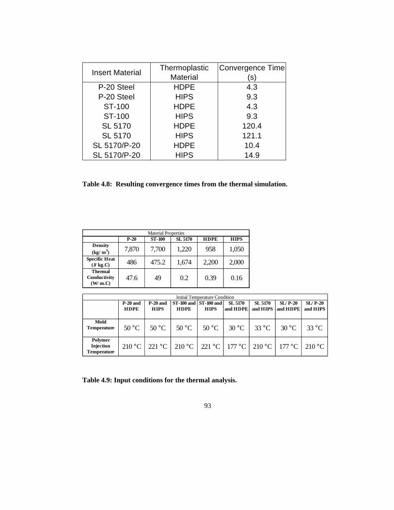
93

Table 4.8: Resulting convergence times from the thermal simulation.

Table 4.9: Input conditions for the thermal analysis.

P-20 ST-100 SL 5170 HDPE HIPSDensity (kg/m3) 7,870 7,700 1,220 958 1,050

Specific Heat (J/kg.C) 486 475.2 1,674 2,200 2,000Thermal

Conductivity (W/m.C)

47.6 49 0.2 0.39 0.16

P-20 and HDPE

P-20 and HIPS

ST-100 and HDPE

ST-100 and HIPS

SL 5170 and HDPE

SL 5170 and HIPS

SL/P-20 and HDPE

SL/P-20 and HIPS

Mold Temperature 50 °C 50 °C 50 °C 50 °C 30 °C 33 °C 30 °C 33 °C

Polymer Injection

Temperature210 °C 221 °C 210 °C 221 °C 177 °C 210 °C 177 °C 210 °C

Material Properties

Initial Temperature Condition

Insert MaterialThermoplastic

MaterialConvergence Time

(s)P-20 Steel HDPE 4.3P-20 Steel HIPS 9.3

ST-100 HDPE 4.3ST-100 HIPS 9.3SL 5170 HDPE 120.4SL 5170 HIPS 121.1

SL 5170/P-20 HDPE 10.4SL 5170/P-20 HIPS 14.9

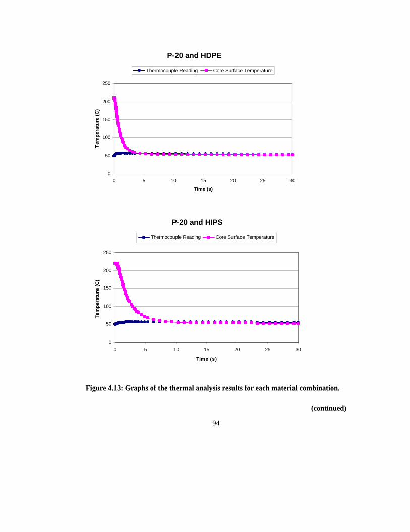
94

P-20 and HDPE

0

50

100

150

200

250

0 5 10 15 20 25 30

Time (s)

Tem

per

atu

re (

C)

Thermocouple Reading Core Surface Temperature

P-20 and HIPS

0

50

100

150

200

250

0 5 10 15 20 25 30

Time (s)

Tem

per

atu

re (

C)

Thermocouple Reading Core Surface Temperature

Figure 4.13: Graphs of the thermal analysis results for each material combination.

(continued)

95

Figure 4.13 (continued.)

ST-100 and HDPE

0

50

100

150

200

250

0 5 10 15 20 25 30

Time (s)

Tem

per

atu

re (

C)

Thermocouple Reading Core Surface Temperature

ST-100 and HIPS

0

50

100

150

200

250

0 5 10 15 20 25 30

Time (s)

Tem

per

atu

re (

C)

Thermocouple Reading Core Surface Temperature

(continued)

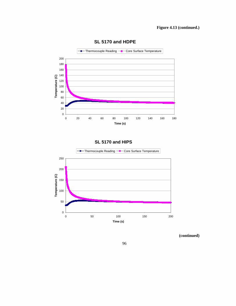
96

Figure 4.13 (continued.)

SL 5170 and HDPE

0

20

40

60

80

100

120

140

160

180

200

0 20 40 60 80 100 120 140 160 180

Time (s)

Tem

per

atu

re (

C)

Thermocouple Reading Core Surface Temperature

SL 5170 and HIPS

0

50

100

150

200

250

0 50 100 150 200

Time (s)

Tem

per

atu

re (

C)

Thermocouple Reading Core Surface Temperature

(continued)

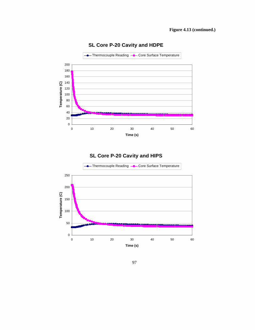
97

Figure 4.13 (continued.)

SL Core P-20 Cavity and HDPE

0

20

40

60

80

100

120

140

160

180

200

0 10 20 30 40 50 60

Time (s)

Tem

per

atu

re (

C)

Thermocouple Reading Core Surface Temperature

SL Core P-20 Cavity and HIPS

0

50

100

150

200

250

0 10 20 30 40 50 60

Time (s)

Tem

per

atu

re (

C)

Thermocouple Reading Core Surface Temperature

98

4.4.2 Ejection Force Measurement

Four Sensotec subminiature load cells, rated at 100 lbs each, were used to

measure ejection force. Each load cell was installed between one of four ejector pins and

the ejector plate. The four pins, mounted on bearings to reduce friction, were attached to

the stripper plate, which removed the canister from the core. Total load was measured

during ejection of each part, and the ejection force was determined from the initial peak

load required to release the part from the insert core. Sample ejection force traces are

shown in Figure 4.14.

After each experimental run, the ejection force was measured without a part on

the core. This no-load ejection force, i.e., the force required to simply move the ejection

mechanism, was subtracted from the peak load measurement of every canister to

determine the actual force required to release the part.

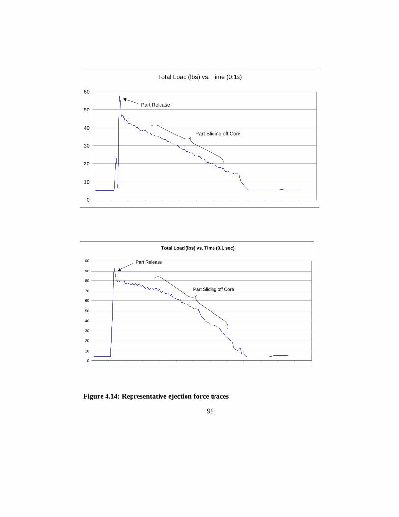
99

Figure 4.14: Representative ejection force traces

Total Load (lbs) vs. Time (0.1s)

0

10

20

30

40

50

60

Part Release

Part Sliding off Core

Total Load (lbs) vs. Time (0.1 sec)

0

10

20

30

40

50

60

70

80

90

100 Part Release

Part Sliding off Core

100

4.4.3 Diameter and Thickness Measurement

The inside and outside diameters of each canister were measured immediately

after ejection to determine the relative change in diameter due to shrinkage and the

canister wall thickness. The relative change in diameter and the thickness measurements

are required in order to use the Menges equation (see Chapter 3). A digital picture of

each canister was taken immediately after ejection (Figure 4.15). A picture including a

scale was taken for each set of experiments. Using Adobe Photoshop® software, the

pictures were magnified and the inside and outside diameters of each canister were

measured in four places: vertically, horizontally, and at 45-degree angles. The four

measurements were averaged for each diameter value. The scale reference picture was

also magnified and measured to determine the number of pixels per inch. The resolution

for each set of measurements varied between 0.0009 and 0.0010 inches per pixel.

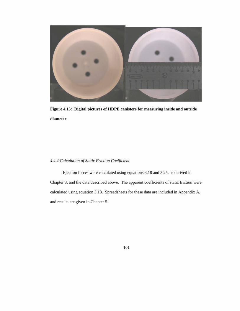
101

Figure 4.15: Digital pictures of HDPE canisters for measuring inside and outside

diameter.

4.4.4 Calculation of Static Friction Coefficient

Ejection forces were calculated using equations 3.18 and 3.25, as derived in

Chapter 3, and the data described above. The apparent coefficients of static friction were

calculated using equation 3.18. Spreadsheets for these data are included in Appendix A,

and results are given in Chapter 5.

102

CHAPTER 5

RESULTS AND ANALYSIS

This chapter summarizes results from the injection molding experiments and

standard friction tests. First, the data from each are discussed individually. Next,

experimental ejection forces are compared with those calculated from the ejection force

model, using friction coefficients from the standard tests. Then, calculations of the

coefficient of static friction, using data from the injection molding experiments, are

presented and compared to standard test results. Analysis of variance results from the

designed experiment are also included. The last section of the chapter presents a

qualitative analysis of the rapid tooled injection mold inserts, i.e., some observations of

how these tools performed.

103

5.1 Injection Molding Experiments

5.1.1 Experimental Results and Discussion

Ejection forces from the injection molding experiments for HDPE and HIPS are

shown in Table 5.1. Measured ejection force results are listed by levels of packing time,

cooling time, and packing pressure. Other experimental data, including diameter and

temperature measurements, are included in Appendix A. The following discussion

comments on the ejection force results according to thermoplastic material and mold

insert material.

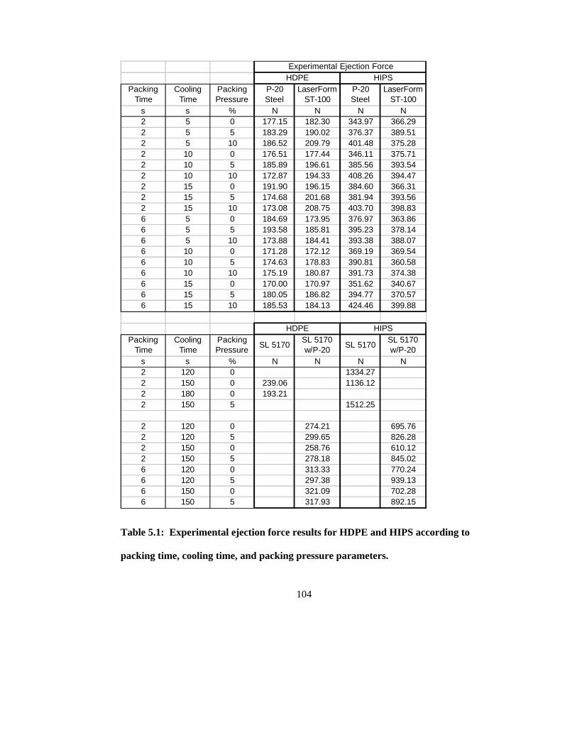
104

Packing Time

Cooling Time

Packing Pressure

P-20 Steel

LaserForm ST-100

P-20 Steel

LaserForm ST-100

s s % N N N N2 5 0 177.15 182.30 343.97 366.292 5 5 183.29 190.02 376.37 389.512 5 10 186.52 209.79 401.48 375.282 10 0 176.51 177.44 346.11 375.712 10 5 185.89 196.61 385.56 393.542 10 10 172.87 194.33 408.26 394.472 15 0 191.90 196.15 384.60 366.312 15 5 174.68 201.68 381.94 393.562 15 10 173.08 208.75 403.70 398.836 5 0 184.69 173.95 376.97 363.866 5 5 193.58 185.81 395.23 378.146 5 10 173.88 184.41 393.38 388.076 10 0 171.28 172.12 369.19 369.546 10 5 174.63 178.83 390.81 360.586 10 10 175.19 180.87 391.73 374.386 15 0 170.00 170.97 351.62 340.676 15 5 180.05 186.82 394.77 370.576 15 10 185.53 184.13 424.46 399.88

Packing Time

Cooling Time

Packing Pressure

SL 5170SL 5170 w/P-20

SL 5170SL 5170 w/P-20

s s % N N N N2 120 0 1334.272 150 0 239.06 1136.122 180 0 193.212 150 5 1512.25

2 120 0 274.21 695.762 120 5 299.65 826.282 150 0 258.76 610.122 150 5 278.18 845.026 120 0 313.33 770.246 120 5 297.38 939.136 150 0 321.09 702.286 150 5 317.93 892.15

Experimental Ejection Force

HDPE HIPS

HDPE HIPS

Table 5.1: Experimental ejection force results for HDPE and HIPS according to

packing time, cooling time, and packing pressure parameters.

105

5.1.2 HDPE Experimental Ejection Force Results

Figure 5.1 shows experimental ejection force results for HDPE. Ejection forces

for HDPE from the P-20 core, averaged per run, are generally lower than from the ST-

100 core, which are lower than from the SL 5170 core. Ejection forces from the ST-100

core at low level packing time are higher than at high level packing time. The parts with

higher ejection force also had lower shrinkage values, as measured by the relative change

in diameter immediately after ejection.

Ejection forces for HDPE from the SL 5170 core with the P-20 cavity are higher

than from the SL 5170 insert because the P-20 cavity draws away much of the heat,

resulting in more shrinkage of the HDPE against the SL 5170 core.

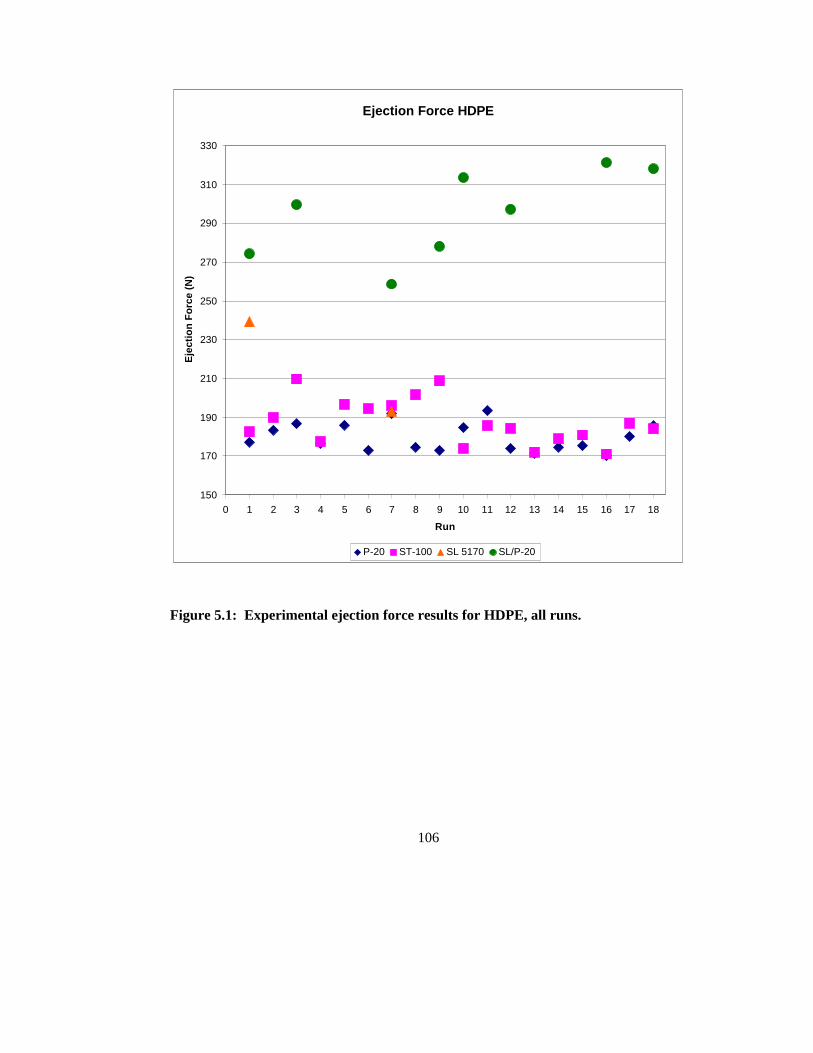
106

Figure 5.1: Experimental ejection force results for HDPE, all runs.

Ejection Force HDPE

150

170

190

210

230

250

270

290

310

330

0 1 2 3 4 5 6 7 8 9 10 11 12 13 14 15 16 17 18

Run

Eje

ctio

n F

orc

e (N

)

P-20 ST-100 SL 5170 SL/P-20

107

5.1.3 HIPS Experimental Ejection Force Results

Figure 5.2 shows experimental ejection force results for HIPS. In contrast to

HDPE, ejection forces from the P-20 core, averaged per run, are greater than from the

ST-100 core for 12 out of 18 runs. Ejection forces from the SL 5170 core are much

higher than from the other two. Also in contrast to HDPE, ejection forces for HIPS from

the SL 5170 insert are larger than those from the combination SL 5170/P-20 insert. This

is because, as will be seen in the standard friction tests, HIPS and SL 5170 react more

strongly with each other at higher temperatures.

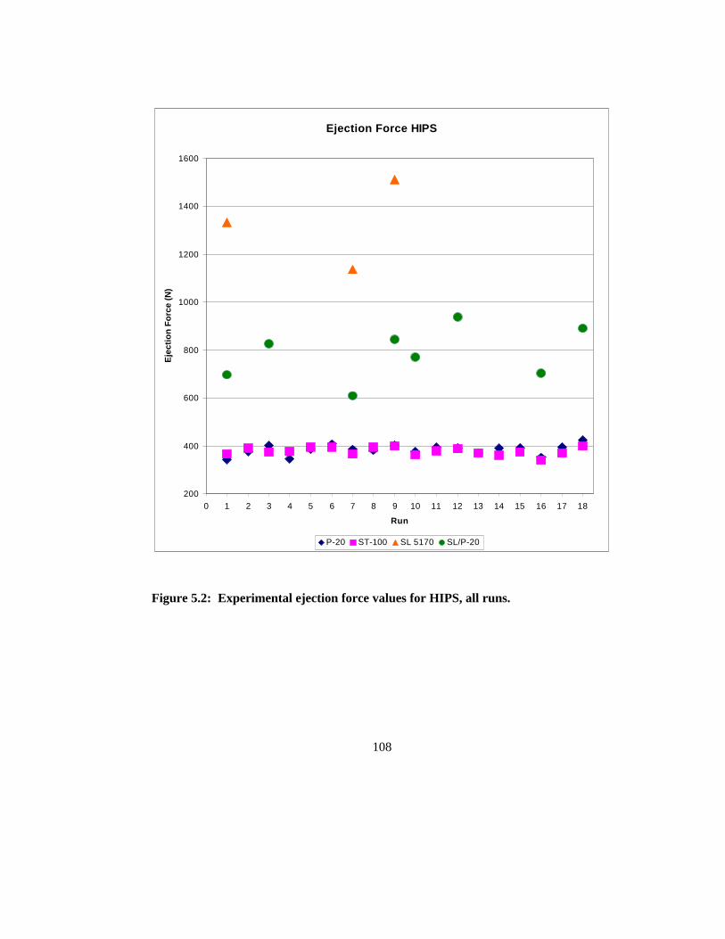
108

Figure 5.2: Experimental ejection force values for HIPS, all runs.

Ejection Force HIPS

200

400

600

800

1000

1200

1400

1600

0 1 2 3 4 5 6 7 8 9 10 11 12 13 14 15 16 17 18

Run

Eje

ctio

n F

orc

e (N

)

P-20 ST-100 SL 5170 SL/P-20

109

5.1.4 Experimental Ejection Force Results from the P-20 and ST-100 Inserts

From both the P-20 and ST-100 inserts, ejection forces for HDPE were lower than

for HIPS for all experimental runs (Figure 5.3).

5.1.5 Experimental Ejection Force Results from the SL 5170 and SL 5170/P-20 Inserts

Due to the problems with cavity deformation and parts sticking in the core, only

two HDPE runs and three HIPS runs were completed with the SL 5170 core and cavity.

With this insert, ejection forces for HIPS were much higher than for HDPE (Figure 5.4).

The same result can be seen from the SL 5170 insert with the P-20 cavity.

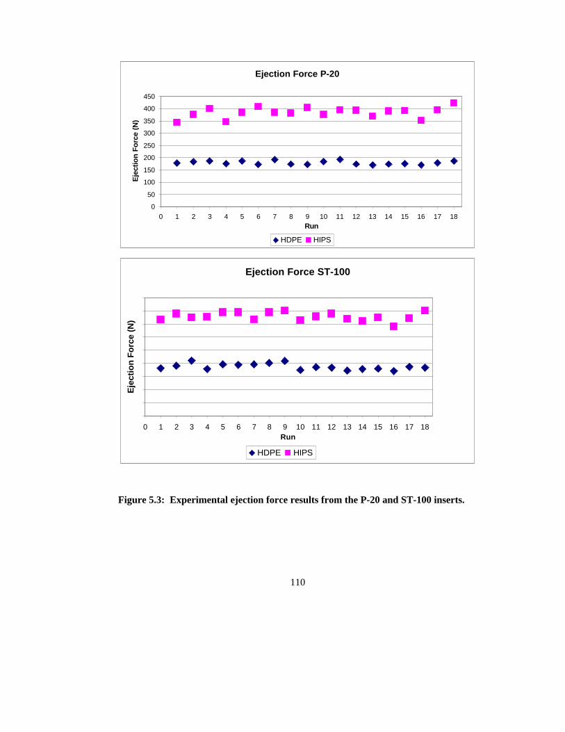
110

Ejection Force P-20

0

50

100

150

200

250

300

350

400

450

0 1 2 3 4 5 6 7 8 9 10 11 12 13 14 15 16 17 18Run

Eje

ctio

n Fo

rce

(N)

HDPE HIPS

Ejection Force ST-100

0 1 2 3 4 5 6 7 8 9 10 11 12 13 14 15 16 17 18Run

Eje

ctio

n F

orc

e (N

)

HDPE HIPS

Figure 5.3: Experimental ejection force results from the P-20 and ST-100 inserts.

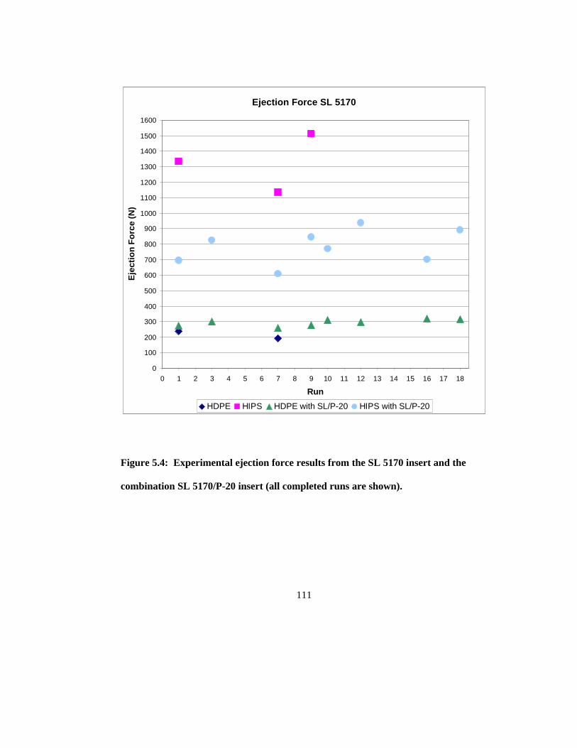
111

Ejection Force SL 5170

0

100

200

300

400

500

600

700

800

900

1000

1100

1200

1300

1400

1500

1600

0 1 2 3 4 5 6 7 8 9 10 11 12 13 14 15 16 17 18

Run

Eje

ctio

n F

orc

e (N

)

HDPE HIPS HDPE with SL/P-20 HIPS with SL/P-20

Figure 5.4: Experimental ejection force results from the SL 5170 insert and the

combination SL 5170/P-20 insert (all completed runs are shown).

112

5.2 Statistical Analysis

5.2.1 DOE Results

Analysis of variance results for the designed experiment described in Chapter 4

are shown in Table 5.2. Numbers are given for the slope of the line that defines the effect

(in Newtons per unit) and the correlation coefficient. The slope of the line indicates the

magnitude of the effect. The correlation coefficient applies only for three-level

parameters and indicates how well the line (defined by the slope) fits the data. If the

correlation coefficient is low, then the effect is not linear. A check mark indicates that

there was an interaction between the parameters shown.

5.2.2 Main Effects and Interactions

As shown in Table 5.2, ejection force increased with packing time for the SL

5170 insert, and decreased with packing time for the ST-100 insert. Packing time also

had an effect from the P-20 insert on the HIPS ejection force, but not on the HDPE

ejection force. Ejection force decreased with cooling time for the P-20 insert. Note that,

for HDPE, the correlation coefficient was low, indicating that the effect was not linear.

Packing pressure had an effect on ejection force for HIPS with the SL 5170 and P-20

inserts, but did not for HDPE. There were no interaction effects for the SL 5170 insert.

The effects on ejection force from these parameters differed between the baseline

steel insert and the rapid tooled inserts. Furthermore, there were differences in effects

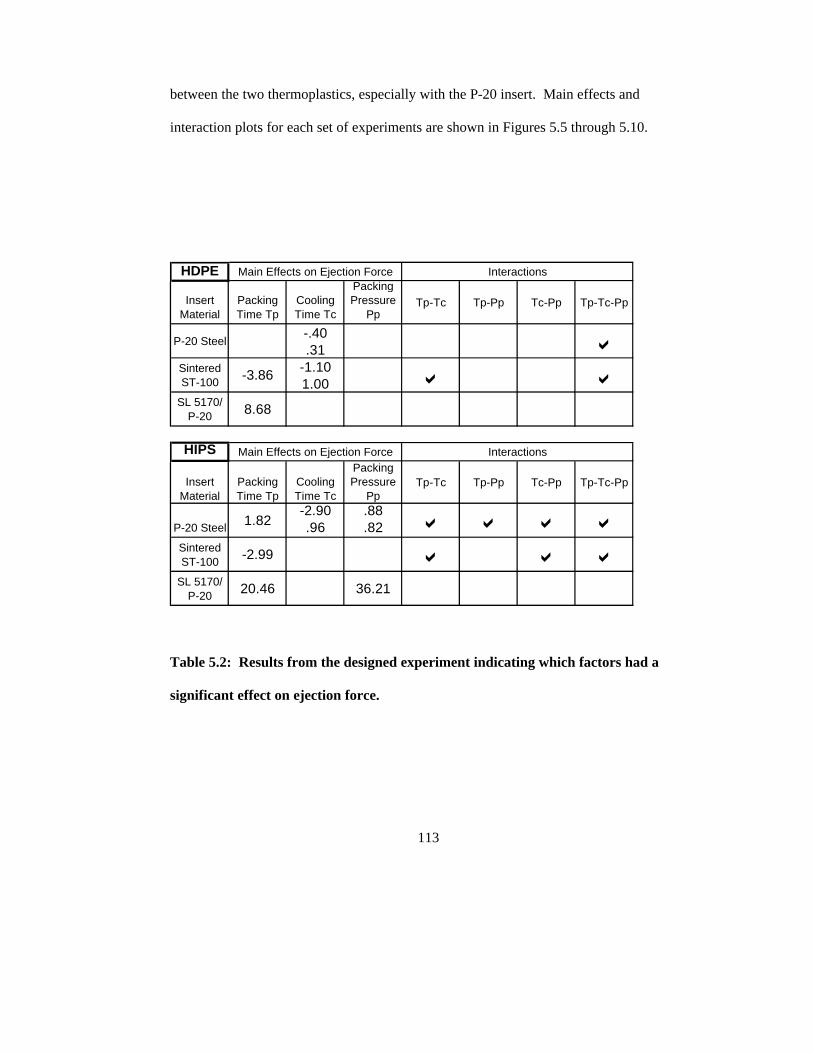
113

between the two thermoplastics, especially with the P-20 insert. Main effects and

interaction plots for each set of experiments are shown in Figures 5.5 through 5.10.

Table 5.2: Results from the designed experiment indicating which factors had a

significant effect on ejection force.

HDPE

Insert Material

Packing Time Tp

Cooling Time Tc

Packing Pressure

PpTp-Tc Tp-Pp Tc-Pp Tp-Tc-Pp

P-20 Steel-.40 .31 a

Sintered ST-100 -3.86 -1.10

1.00 a aSL 5170/

P-20 8.68

HIPS

Insert Material

Packing Time Tp

Cooling Time Tc

Packing Pressure

PpTp-Tc Tp-Pp Tc-Pp Tp-Tc-Pp

P-20 Steel 1.82-2.90 .96

.88

.82 a a a aSintered ST-100 -2.99 a a a

SL 5170/ P-20 20.46 36.21

Main Effects on Ejection Force Interactions

Main Effects on Ejection Force Interactions

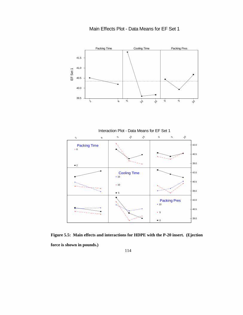
114

Packing PresCooling TimePacking Time

10 5 01510 562

41.5

41.0

40.5

40.0

39.5

EF

Set

1

Main Effects Plot - Data Means for EF Set 1

10 5 01510 562

42.0

40.5

39.0

42.0

40.5

39.0

42.0

40.5

39.0

Packing Time

Cooling Time

Packing Pres10

5

0

15

10

5

6

2

Interaction Plot - Data Means for EF Set 1

Figure 5.5: Main effects and interactions for HDPE with the P-20 insert. (Ejection

force is shown in pounds.)

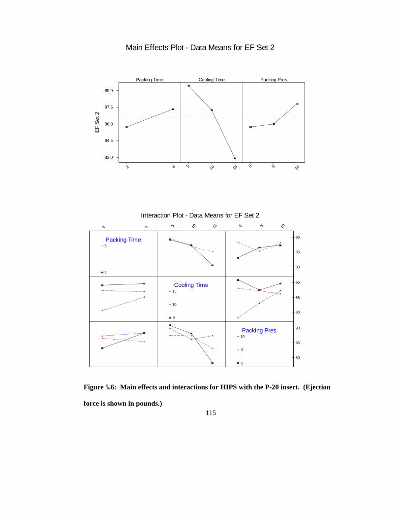
115

Packing Time Cooling Time Packing Pres

2 6 5 10 15 0 5 10

83.0

84.5

86.0

87.5

89.0

EF

Set

2

Main Effects Plot - Data Means for EF Set 2

2 6 5 10 15 0 5 10

80

85

90

80

85

90

80

85

90Packing Time

Cooling Time

Packing Pres

2

6

5

10

15

0

5

10

Interaction Plot - Data Means for EF Set 2

Figure 5.6: Main effects and interactions for HIPS with the P-20 insert. (Ejection

force is shown in pounds.)

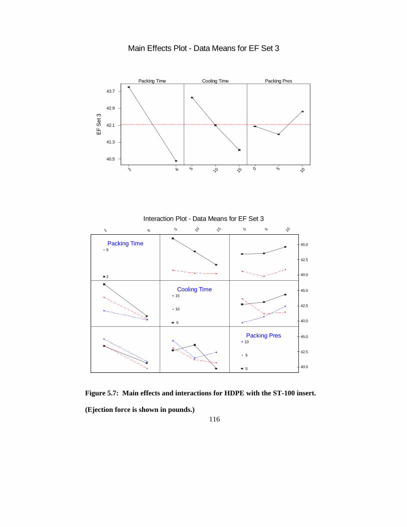
116

Packing Time Cooling Time Packing Pres

2 6 5 10 15 0 5 10

40.5

41.3

42.1

42.9

43.7

EF

Set

3

Main Effects Plot - Data Means for EF Set 3

10 5 01510 562

45.0

42.5

40.0

45.0

42.5

40.0

45.0

42.5

40.0

Packing Time

Cooling Time

Packing Pres10

5

0

15

10

5

6

2

Interaction Plot - Data Means for EF Set 3

Figure 5.7: Main effects and interactions for HDPE with the ST-100 insert.

(Ejection force is shown in pounds.)

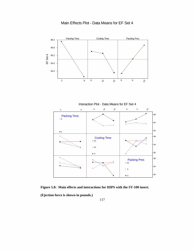
117

Packing Time Cooling Time Packing Pres

2 6 5 10 15 0 5 10

84.0

84.6

85.2

85.8

86.4

EF

Set

4

Main Effects Plot - Data Means for EF Set 4

2 6 5 10 15 0 5 10

80

84

88

80

84

88

80

84

88Packing Time

Cooling Time

Packing Pres

2

6

5

10

15

0

5

10

Interaction Plot - Data Means for EF Set 4

Figure 5.8: Main effects and interactions for HIPS with the ST-100 insert.

(Ejection force is shown in pounds.)

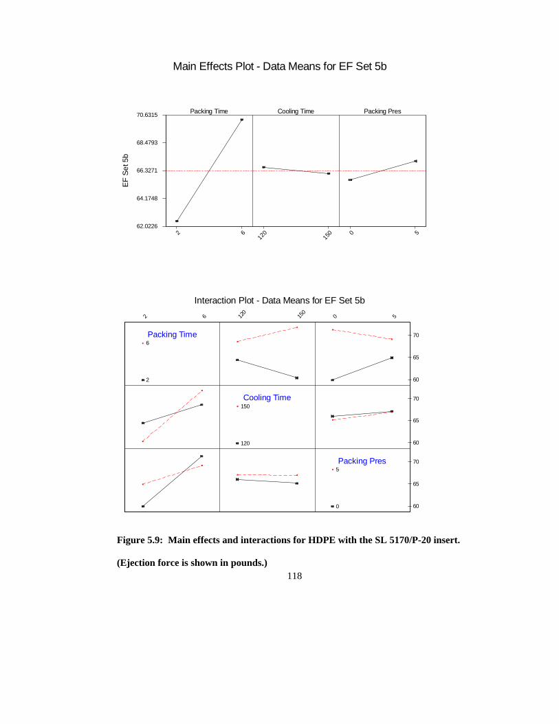
118

Packing Time Cooling Time Packing Pres

2 612

015

0 0 562.0226

64.1748

66.3271

68.4793

70.6315

EF

Set

5b

Main Effects Plot - Data Means for EF Set 5b

2 6 120

150

0 5

60

65

70

60

65

70

60

65

70Packing Time

Cooling Time

Packing Pres

2

6

120

150

0

5

Interaction Plot - Data Means for EF Set 5b

Figure 5.9: Main effects and interactions for HDPE with the SL 5170/P-20 insert.

(Ejection force is shown in pounds.)

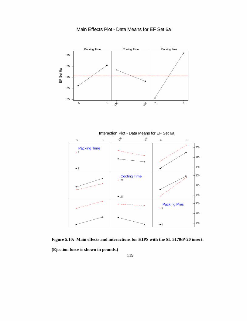
119

Packing Time Cooling Time Packing Pres

2 612

015

0 0 5

155

165

175

185

195

EF

Set

6a

Main Effects Plot - Data Means for EF Set 6a

2 6 120

150

0 5

150

175

200

150

175

200

150

175

200Packing Time

Cooling Time

Packing Pres

2

6

120

150

0

5

Interaction Plot - Data Means for EF Set 6a

Figure 5.10: Main effects and interactions for HIPS with the SL 5170/P-20 insert.

(Ejection force is shown in pounds.)

120

5.3 Standard Friction Testing Results

Coefficient of friction results from the standard tests are shown in Figures 5.11

and 5.12. In general the data show some expected trends. For example, at room

temperature, the friction coefficient of HIPS is larger than that of HDPE on all three plate

materials. Also, the friction coefficients of both thermoplastics on the SL 5170 plate are

higher than those on the metal plates.

5.3.1 HDPE Standard Friction Results

Temperature did not make a dramatic difference in friction coefficient for HDPE

on P-20, ST-100, or SL 5170. For the P-20 plate, the difference in coefficient between

temperatures was not statistically significant. With the ST-100 and SL 5170 plates, there

was an increase in the friction coefficient in the ejection temperature tests as compared to

the room temperature tests. This is probably because the adhesion component of friction

became more apparent in the heated tests. From ejection temperature to elevated

temperature for the ST-100 plate, the difference in the coefficient of friction was not

statistically significant. For the SL 5170 plate, there was actually a slight decrease in

friction coefficient from ejection temperature to elevated temperature, an unexpected

result.

In all cases, elevating the initial temperature to imprint the surface of the

specimen was presumed to increase the friction coefficient. This was not the case for any

of the HDPE tests. No change in coefficient (in the case of P-20 and ST-100) and the

slight decrease in coefficient (in the case of SL 5170) may be due to shrinkage of the sled

121

specimen from the plate and a reduction in the area of contact due to the imprinted

pattern. HDPE is a crystalline polymer and will shrink more than HIPS, which is an

amorphous polymer. As discussed in Chapter 3, compared to amorphous materials, a

crystalline structure can arrange itself into a tighter, more orderly fashion as the polymer

cools. It is noted, however, that the imprinted pattern was not very pronounced on the

HDPE specimens. Therefore, the temperature to which the specimens were heated was

probably not high enough to sufficiently soften the polymer.

The relationship of HDPE friction coefficients among the three plate materials

was as expected. The coefficients for HDPE on SL 5170 were highest because of the

nature of polymer on polymer materials and because the surface roughness of this plate

was higher than that of the other two. The coefficients of HDPE on ST-100 were lowest

because the surface roughness of this plate was lower than that of the other two. The

conductivity of the ST-100 plate is also highest, which may have contributed to a

reduction in adhesion by dissipating heat at a faster rate in the heated tests.

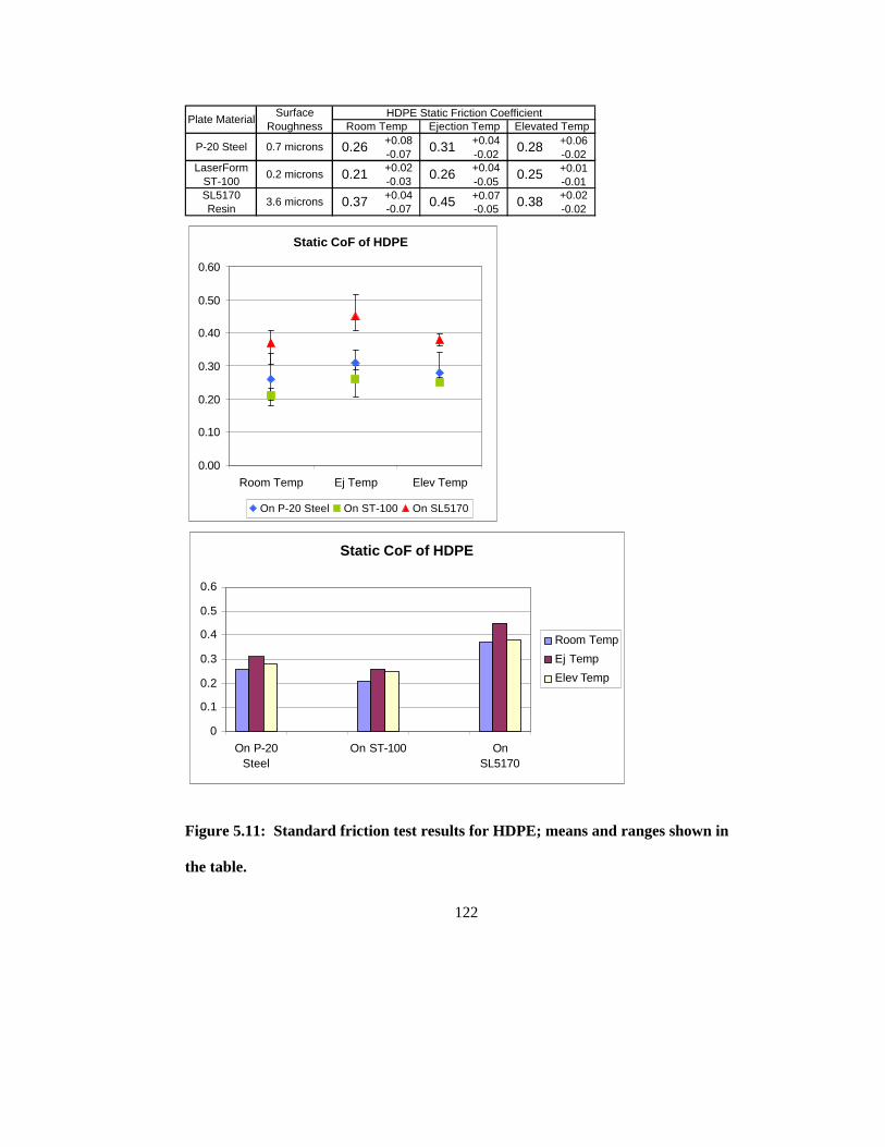
122

Figure 5.11: Standard friction test results for HDPE; means and ranges shown in

the table.

Static CoF of HDPE

0

0.1

0.2

0.3

0.4

0.5

0.6

On P-20Steel

On ST-100 OnSL5170

Room Temp

Ej Temp

Elev Temp

+0.08 +0.04 +0.06-0.07 -0.02 -0.02+0.02 +0.04 +0.01-0.03 -0.05 -0.01+0.04 +0.07 +0.02-0.07 -0.05 -0.02

Room Temp Ejection Temp Elevated Temp

0.26

0.21

0.37

0.31

0.26

0.45

0.28

SL5170 Resin

3.6 microns

0.25

0.38

LaserForm ST-100

0.2 microns

P-20 Steel 0.7 microns

HDPE Static Friction CoefficientPlate MaterialSurface

Roughness

Static CoF of HDPE

0.00

0.10

0.20

0.30

0.40

0.50

0.60

Room Temp Ej Temp Elev Temp

On P-20 Steel On ST-100 On SL5170

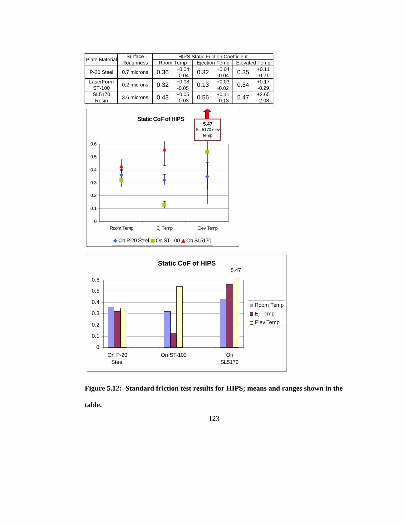
123

Figure 5.12: Standard friction test results for HIPS; means and ranges shown in the

table.

Static CoF of HIPS5.47

0

0.1

0.2

0.3

0.4

0.5

0.6

On P-20Steel

On ST-100 OnSL5170

Room Temp

Ej Temp

Elev Temp

+0.04 +0.04 +0.11-0.04 -0.04 -0.21+0.08 +0.03 +0.17-0.05 -0.02 -0.29+0.05 +0.11 +2.65-0.03 -0.13 -2.08

HIPS Static Friction CoefficientRoom Temp Ejection Temp Elevated Temp

LaserForm ST-100

0.2 microns

SL5170 Resin

3.6 microns

Plate MaterialSurface

Roughness

P-20 Steel 0.7 microns 0.36

0.32

0.32

0.13

0.35

0.54

0.43 0.56 5.47

Static CoF of HIPS5.47

SL 5170 elev temp

0

0.1

0.2

0.3

0.4

0.5

0.6

Room Temp Ej Temp Elev Temp

On P-20 Steel On ST-100 On SL5170

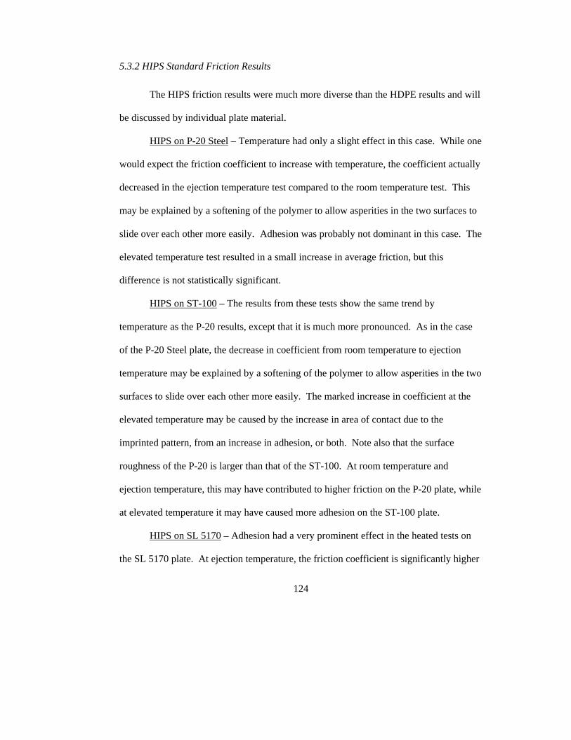
124

5.3.2 HIPS Standard Friction Results

The HIPS friction results were much more diverse than the HDPE results and will

be discussed by individual plate material.

HIPS on P-20 Steel – Temperature had only a slight effect in this case. While one

would expect the friction coefficient to increase with temperature, the coefficient actually

decreased in the ejection temperature test compared to the room temperature test. This

may be explained by a softening of the polymer to allow asperities in the two surfaces to

slide over each other more easily. Adhesion was probably not dominant in this case. The

elevated temperature test resulted in a small increase in average friction, but this

difference is not statistically significant.

HIPS on ST-100 – The results from these tests show the same trend by

temperature as the P-20 results, except that it is much more pronounced. As in the case

of the P-20 Steel plate, the decrease in coefficient from room temperature to ejection

temperature may be explained by a softening of the polymer to allow asperities in the two

surfaces to slide over each other more easily. The marked increase in coefficient at the

elevated temperature may be caused by the increase in area of contact due to the

imprinted pattern, from an increase in adhesion, or both. Note also that the surface

roughness of the P-20 is larger than that of the ST-100. At room temperature and

ejection temperature, this may have contributed to higher friction on the P-20 plate, while

at elevated temperature it may have caused more adhesion on the ST-100 plate.

HIPS on SL 5170 – Adhesion had a very prominent effect in the heated tests on

the SL 5170 plate. At ejection temperature, the friction coefficient is significantly higher

125

than at room temperature. Whereas the softened polymer slid over the metal plates with

less resistance, it adhered to the resin plate, causing a larger peak frictional force. The

elevated temperature test shows an extreme case of this adhesion, due to a strong

interaction between the two materials. Secondary forces such as dispersion forces,

polarity, or hydrogen bonding, contribute to this interaction. Adhesion between two

materials, for example, will be maximized when their polarities are similar. While the

imprinted pattern of the SL 5170 plate into the softened HIPS material may also have

contributed to the spike in frictional force, the mechanical interaction was not a dominant

influence.

Figure 5.13 shows a sample plot from the HIPS on SL 5170 test. The graph

shows an initial large peak followed by a lower peak as the specimen begins to slide. The

initial peak may be explained by the strong force required to overcome adhesion,

followed by a lesser force required to overcome roughness once the specimen is

“unstuck.” The HIPS on SL 5170 at elevated temperature was the only test to show this

phenomenon. The secondary molecular forces that caused HIPS and SL 5170 to adhere

to each other were not a prominent factor with other material pairs. Polarity has no effect

between HIPS and the two metal plates, because the metal plates become oxidized, and

there is an insulating layer between the polymer specimen and the plate. Polarity has no

effect between HDPE and any of the plates because HDPE is a nonpolar material. Other

test results looked more like the sample HIPS on P-20 graph shown in Figure 5.14.

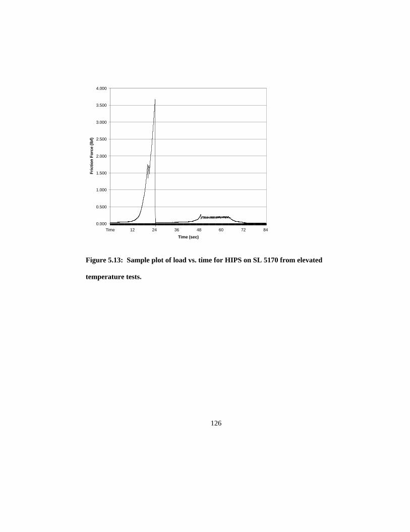
126

Figure 5.13: Sample plot of load vs. time for HIPS on SL 5170 from elevated

temperature tests.

0.000

0.500

1.000

1.500

2.000

2.500

3.000

3.500

4.000

Time 12 24 36 48 60 72 84

Time (sec)

Fri

ctio

n F

orc

e (lb

f)

127

Figure 5.14: Sample plot of load vs. time for HIPS on P-20 from elevated

temperature tests.

The relationship of HIPS friction coefficients among the three plate materials was

as expected, except for the elevated temperature test on ST-100 compared to P-20 Steel.

One would anticipate that the coefficient of friction on ST-100 would be lower because

its surface roughness is lower than that of the P-20. Instead, however, the smoother

finish may have allowed the adhesion component of friction to dominate in this case. In

the room temperature and ejection temperature cases, the friction coefficient of HIPS on

ST-100 was lowest, and in all cases the friction coefficient of HIPS on SL 5170 was

highest.

0.000

0.050

0.100

0.150

0.200

0.250

Time 12 24 36 48 60 72 84

Time (sec)

Fric

tion

Forc

e (lb

f)

128

5.4 Reliability of the Data

In conjunction with the experimental and test discussions above, a few parameter

discrepancies and data variations must be noted. First, there are differences in injection

molding process parameters among experimental sets. These are necessary because of

the nature of the materials used. For example, HDPE and HIPS have different processing

temperatures and injection velocities. Also, the temperatures and pressures used with the

SL 5170 resin mold insert are as low as the processing window will allow so that minimal

deformation or degradation occurs. A complete list of process parameters is included in

Chapter 4.

Second, there may be some variation in the data due to the following:

• HDPE parts were flared slightly at the rim in ejections from the P-20 and ST-100

cores. This flaring occurred due to the magnitude of the ejection force applied by

the stripper plate and the softness of the warm thermoplastic material. This

flaring may have increased canister diameter measurements slightly, and can

affect ejection force calculations.

• The SL 5170 core was susceptible to swelling. Experiments with the SL 5170

core and the P-20 cavity were run with significantly lower ejection temperature

because, if the heat was increased to raise ejection temperature, then core swelling

was excessive. Core swelling may have affected diameter measurements as well.

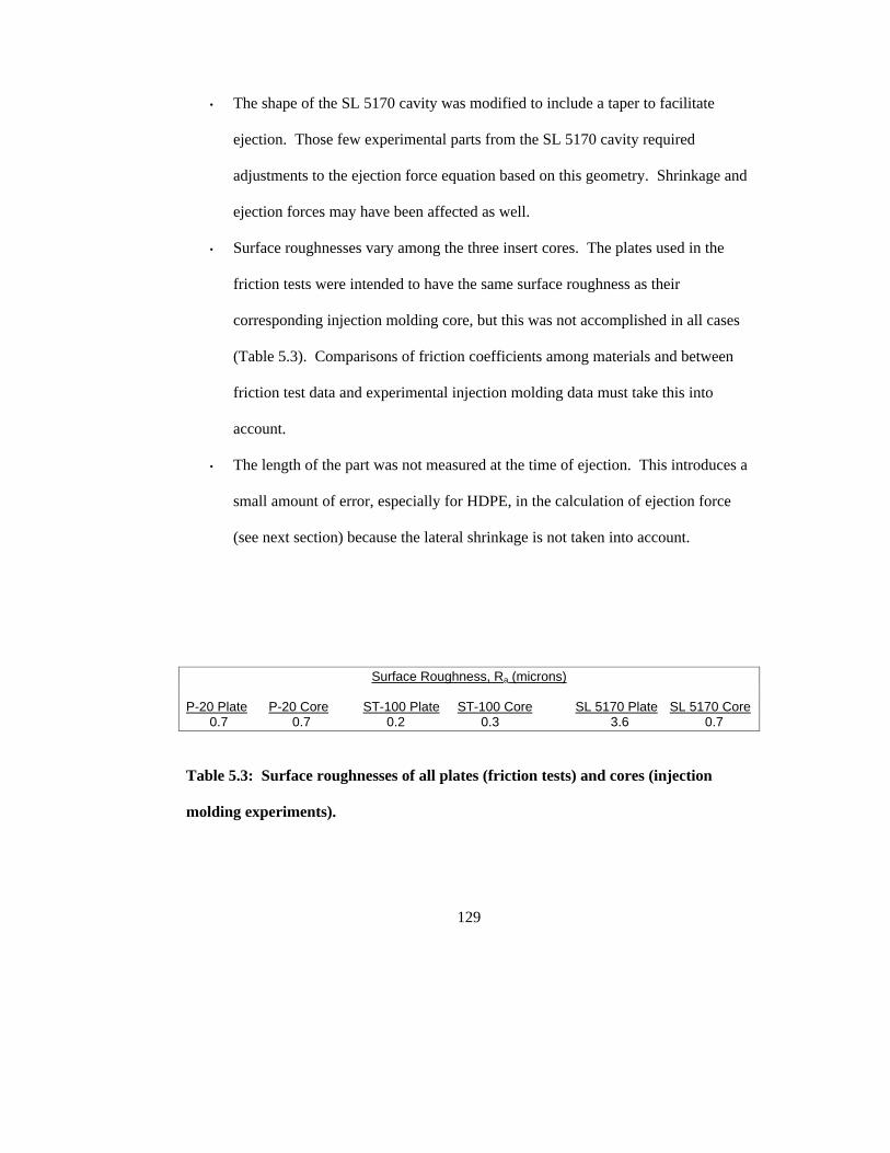
129

• The shape of the SL 5170 cavity was modified to include a taper to facilitate

ejection. Those few experimental parts from the SL 5170 cavity required

adjustments to the ejection force equation based on this geometry. Shrinkage and

ejection forces may have been affected as well.

• Surface roughnesses vary among the three insert cores. The plates used in the

friction tests were intended to have the same surface roughness as their

corresponding injection molding core, but this was not accomplished in all cases

(Table 5.3). Comparisons of friction coefficients among materials and between

friction test data and experimental injection molding data must take this into

account.

• The length of the part was not measured at the time of ejection. This introduces a

small amount of error, especially for HDPE, in the calculation of ejection force

(see next section) because the lateral shrinkage is not taken into account.

Surface Roughness, R a (microns)

P-20 Plate P-20 Core ST-100 Plate ST-100 Core SL 5170 Plate SL 5170 Core 0.7 0.7 0.2 0.3 3.6 0.7

Table 5.3: Surface roughnesses of all plates (friction tests) and cores (injection

molding experiments).

130

5.5 Calculation of Ejection Force Using the Model

Using the values for coefficient of static friction from the standard tests at

elevated temperature, ejection forces have been calculated using the Menges model

derived in Chapter 3. These values, along with the experimental values for ejection

force, are shown in Tables 5.4 and 5.5. The difference between calculated values and

actual experimental values for ejection force is significant, and excessive in some of the

HIPS cases.

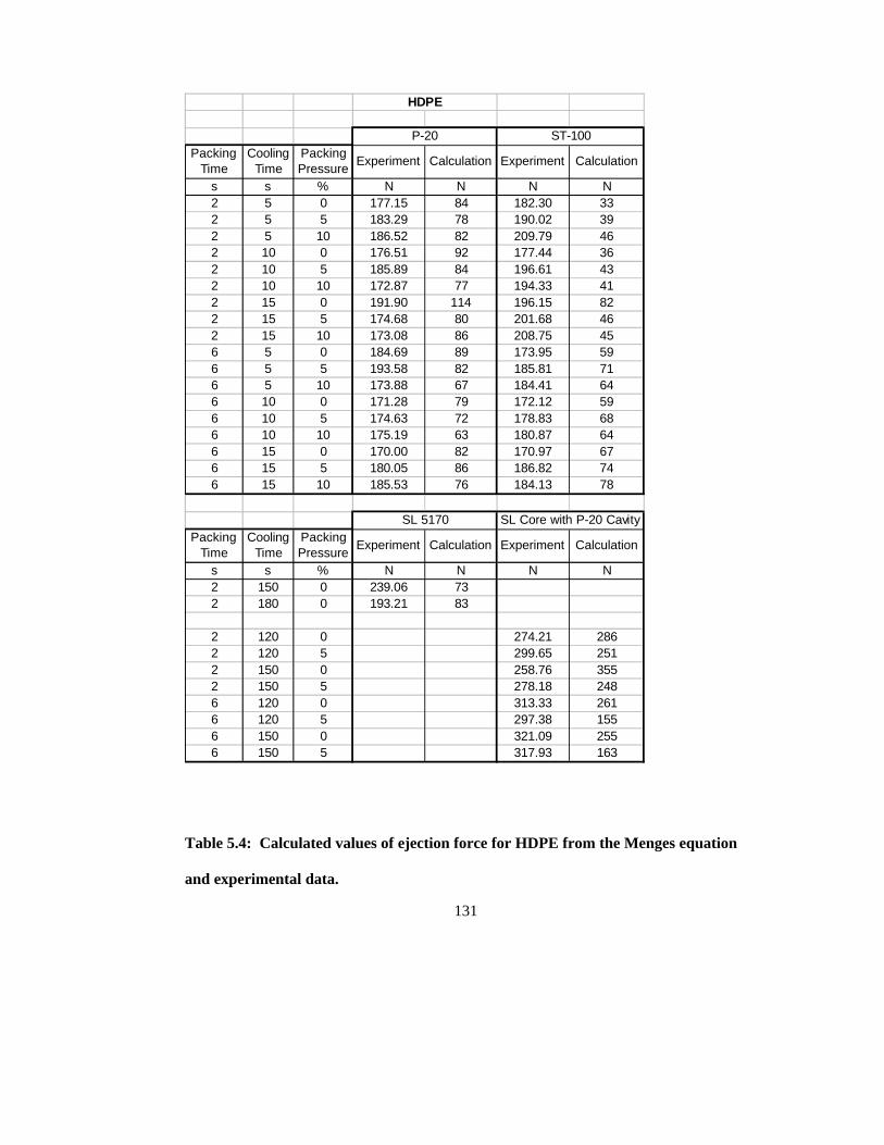
131

Packing Time

Cooling Time

Packing Pressure

Experiment Calculation Experiment Calculation

s s % N N N N2 5 0 177.15 84 182.30 332 5 5 183.29 78 190.02 392 5 10 186.52 82 209.79 462 10 0 176.51 92 177.44 362 10 5 185.89 84 196.61 432 10 10 172.87 77 194.33 412 15 0 191.90 114 196.15 822 15 5 174.68 80 201.68 462 15 10 173.08 86 208.75 456 5 0 184.69 89 173.95 596 5 5 193.58 82 185.81 716 5 10 173.88 67 184.41 646 10 0 171.28 79 172.12 596 10 5 174.63 72 178.83 686 10 10 175.19 63 180.87 646 15 0 170.00 82 170.97 676 15 5 180.05 86 186.82 746 15 10 185.53 76 184.13 78

Packing Time

Cooling Time

Packing Pressure

Experiment Calculation Experiment Calculation

s s % N N N N2 150 0 239.06 732 180 0 193.21 83

2 120 0 274.21 2862 120 5 299.65 2512 150 0 258.76 3552 150 5 278.18 2486 120 0 313.33 2616 120 5 297.38 1556 150 0 321.09 2556 150 5 317.93 163

HDPE

SL 5170 SL Core with P-20 Cavity

P-20 ST-100

Table 5.4: Calculated values of ejection force for HDPE from the Menges equation

and experimental data.

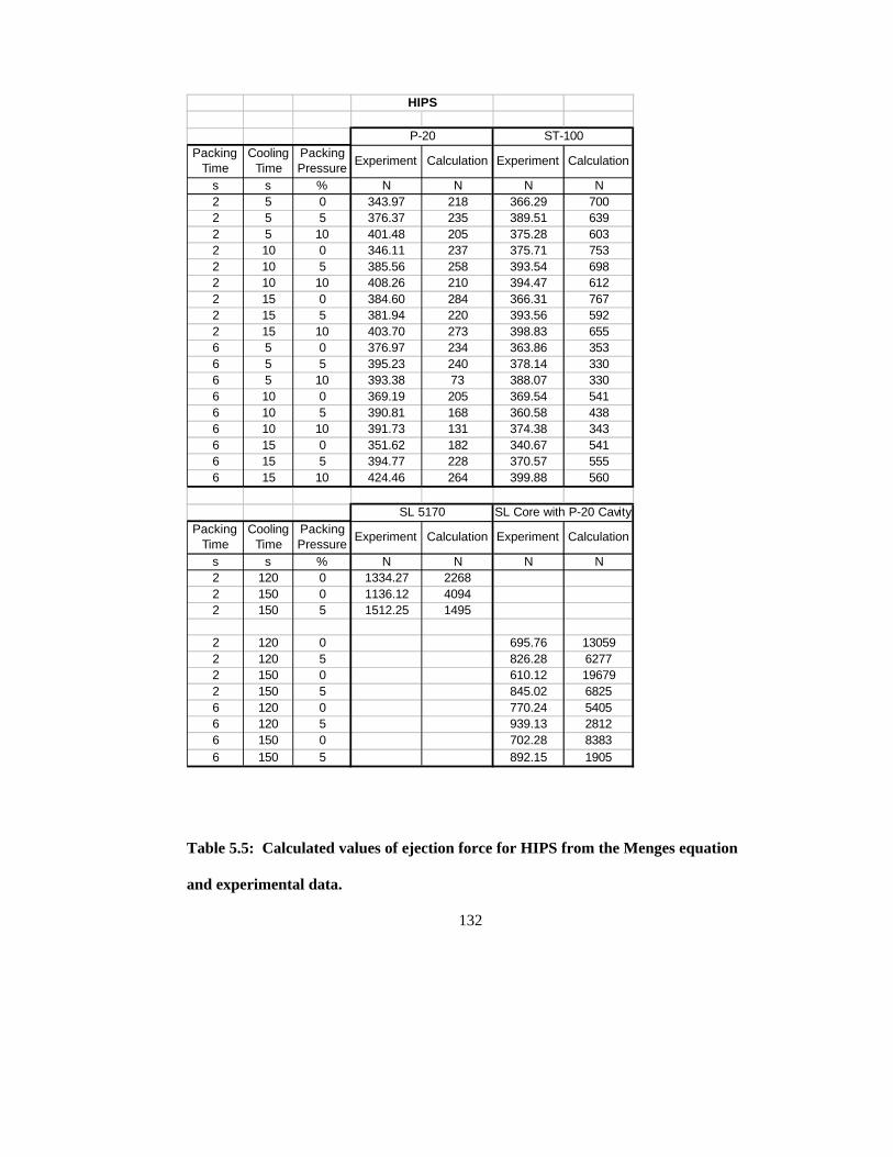
132

Packing Time

Cooling Time

Packing Pressure

Experiment Calculation Experiment Calculation

s s % N N N N2 5 0 343.97 218 366.29 7002 5 5 376.37 235 389.51 6392 5 10 401.48 205 375.28 6032 10 0 346.11 237 375.71 7532 10 5 385.56 258 393.54 6982 10 10 408.26 210 394.47 6122 15 0 384.60 284 366.31 7672 15 5 381.94 220 393.56 5922 15 10 403.70 273 398.83 6556 5 0 376.97 234 363.86 3536 5 5 395.23 240 378.14 3306 5 10 393.38 73 388.07 3306 10 0 369.19 205 369.54 5416 10 5 390.81 168 360.58 4386 10 10 391.73 131 374.38 3436 15 0 351.62 182 340.67 5416 15 5 394.77 228 370.57 5556 15 10 424.46 264 399.88 560

Packing Time

Cooling Time

Packing Pressure

Experiment Calculation Experiment Calculation

s s % N N N N2 120 0 1334.27 22682 150 0 1136.12 40942 150 5 1512.25 1495

2 120 0 695.76 130592 120 5 826.28 62772 150 0 610.12 196792 150 5 845.02 68256 120 0 770.24 54056 120 5 939.13 28126 150 0 702.28 83836 150 5 892.15 1905

HIPS

SL 5170 SL Core with P-20 Cavity

P-20 ST-100

Table 5.5: Calculated values of ejection force for HIPS from the Menges equation

and experimental data.

133

5.5.1 Calculated Ejection Force for HDPE

Figure 5.15 shows that the calculated values for ejection force for HDPE from the

Menges model are lower than the measured values by 50 to 70 percent on average, except

for those from the SL 5170 core with the P-20 cavity. Based on results from the standard

friction test at elevated temperature, the calculated values for ejection force were

expected to be lower than the actual values because, as previously mentioned, the

elevated temperature was probably not high enough to measure an accurate value of the

coefficient of static friction for HDPE. Furthermore, the standard test environment was

not identical to the injection molding environment in terms of temperatures and pressures

and their respective histories.

Calculated ejection force values for HDPE from the SL 5170 core with the P-20

cavity were closer to actuals, i.e., within 16 percent on average. This is because the

ejection temperatures during these experiments were lower than the others, so the friction

coefficient from the standard test is more comparable.

134

Ejection Force HDPE

SL/P-20 SL 5170ST-100P-200

50

100

150

200

250

300

350

400

N

Experimental Calculated

Figure 5.15: Calculated values for ejection force for HPDE using the Menges model

compared with experimental values, averaged across all runs.

5.5.2 Calculated Ejection Force for HIPS

Calculated values for ejection force, averaged across all runs, for HIPS parts from

the P-20 and ST-100 cores are shown with experimental values in Figure 5.16. Those

from the SL 5170 insert, and the SL 5170 core with the P-20 cavity are shown in Figure

5.17. The model estimated ejection force for HIPS on P-20 to be 44 percent lower than

135

actuals, and on ST-100 to be 47 percent higher on average. For the SL 5170 core,

calculated values were higher on average than actual values by 97 percent. (Note that

only three runs of data were collected for the SL 5170 insert.) For the SL 5170 core with

the P-20 cavity, calculated values were extremely high (924 percent higher than actuals).

As was shown for HDPE, differences between calculated and actual ejection force

values for HIPS are due in part to friction coefficients, which vary between standard

measurements and actual ejection. Assuming this to be a primary reason for the

differences in calculated and actual ejection forces, the measured friction coefficient for

HIPS with P-20 was low, and the measured friction coefficients for HIPS with ST-100

and HIPS with SL 5170 were high. In any case, the surface interactions of each material

pair were different during the standard tests as compared to during the injection molding

experiments. Therefore the friction coefficient measured in the standard test caused some

error in the calculation of ejection force when applied to the injection molding case.

5.5.3 Possible Sources of Error

One source of error in the calculation of ejection force using the model developed

by Menges is the coefficient of friction measurement. As mentioned above, the

environment of the standard friction test is not identical to the environment of the

injection molding experiment. Therefore, it is likely that the standard measurement of

the coefficient of friction, even at elevated temperature, is not accurate.

Another possible source of error in the ejection force calculation is the elastic

modulus measurement. Again, the environment of the standard modulus measurement

136

does not exactly simulate the injection molding environment, so there is likely to be some

error. Furthermore, the elastic modulus of the HIPS material is more sensitive to

temperature as compared with HDPE. A small difference between the measured and

actual temperatures in the modulus measurements described in Chapter 4 or in the

injection molding experiments would cause a significant change in elastic modulus and a

resultant change in the calculation of ejection force.

A third source of error in the ejection force calculation is the measurement of the

relative change in diameter of the part. The digital imaging approach used to measure the

inside and outside diameters of the part was probably the most accurate method short of a

laser-based, real time, and much more expensive system. However, digital imaging

required manual transfer of the part from the injection molding machine to the camera

fixture and most likely introduced some error by expanding the time between ejection

and capture of the digital data.

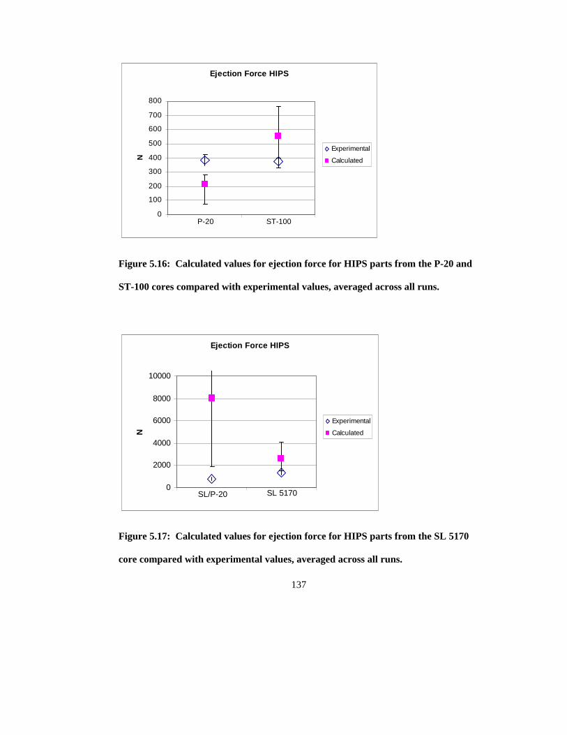
137

Ejection Force HIPS

ST-100P-200

100

200

300

400

500

600

700

800

NExperimental

Calculated

Figure 5.16: Calculated values for ejection force for HIPS parts from the P-20 and

ST-100 cores compared with experimental values, averaged across all runs.

Ejection Force HIPS

SL 5170SL/P-200

2000

4000

6000

8000

10000

N

Experimental

Calculated

Figure 5.17: Calculated values for ejection force for HIPS parts from the SL 5170

core compared with experimental values, averaged across all runs.

138

5.6 Calculation of Apparent Friction Coefficients using the Menges Model

By rearranging the Menges model equation, and using experimental ejection force

and shrinkage data, the apparent coefficient of static friction was calculated for each

material combination. Table 5.7 lists the calculated values by experimental parameters.

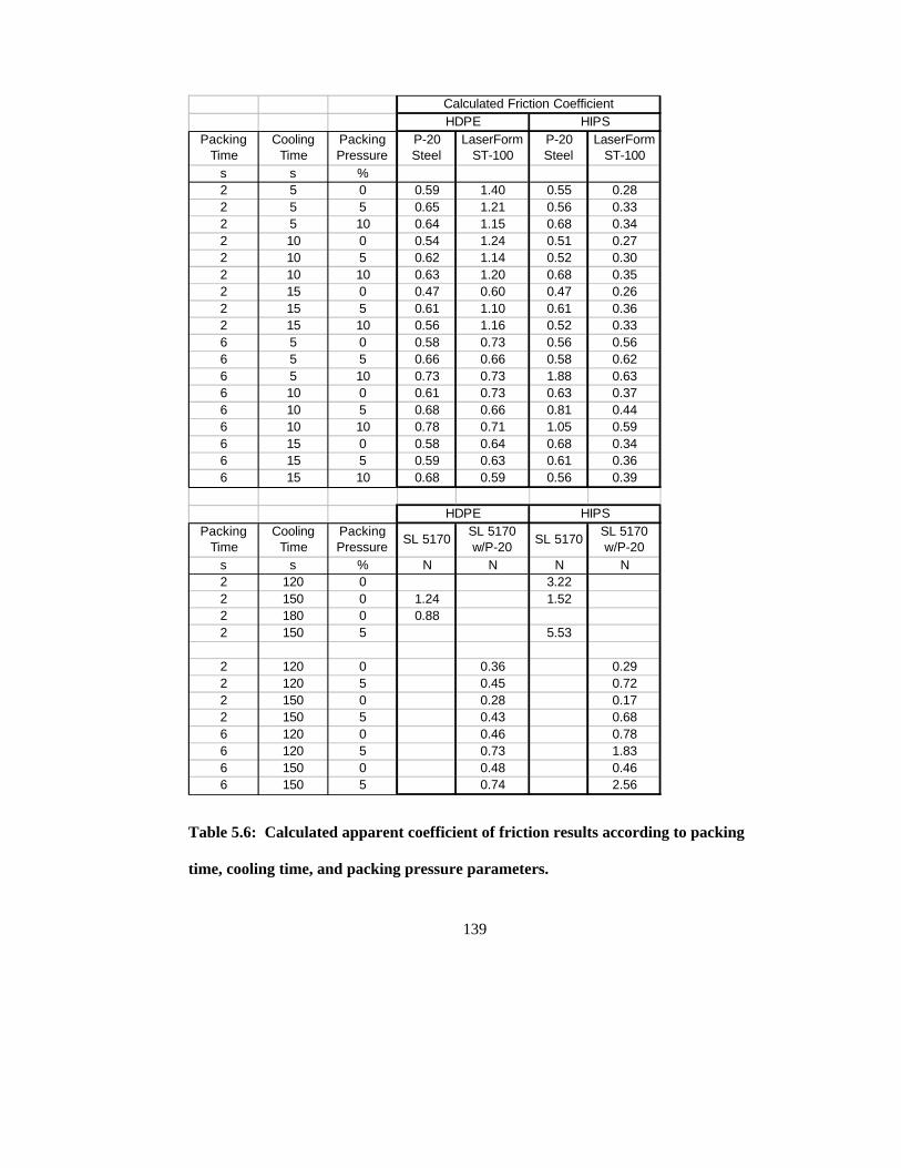
139

Packing Time

Cooling Time

Packing Pressure

P-20 Steel

LaserForm ST-100

P-20 Steel

LaserForm ST-100

s s %2 5 0 0.59 1.40 0.55 0.282 5 5 0.65 1.21 0.56 0.332 5 10 0.64 1.15 0.68 0.342 10 0 0.54 1.24 0.51 0.272 10 5 0.62 1.14 0.52 0.302 10 10 0.63 1.20 0.68 0.352 15 0 0.47 0.60 0.47 0.262 15 5 0.61 1.10 0.61 0.362 15 10 0.56 1.16 0.52 0.336 5 0 0.58 0.73 0.56 0.566 5 5 0.66 0.66 0.58 0.626 5 10 0.73 0.73 1.88 0.636 10 0 0.61 0.73 0.63 0.376 10 5 0.68 0.66 0.81 0.446 10 10 0.78 0.71 1.05 0.596 15 0 0.58 0.64 0.68 0.346 15 5 0.59 0.63 0.61 0.366 15 10 0.68 0.59 0.56 0.39

Packing Time

Cooling Time

Packing Pressure

SL 5170SL 5170 w/P-20

SL 5170SL 5170 w/P-20

s s % N N N N2 120 0 3.222 150 0 1.24 1.522 180 0 0.882 150 5 5.53

2 120 0 0.36 0.292 120 5 0.45 0.722 150 0 0.28 0.172 150 5 0.43 0.686 120 0 0.46 0.786 120 5 0.73 1.836 150 0 0.48 0.466 150 5 0.74 2.56

Calculated Friction Coefficient

HDPE HIPS

HDPE HIPS

Table 5.6: Calculated apparent coefficient of friction results according to packing

time, cooling time, and packing pressure parameters.

140

5.6.1 HDPE Apparent Coefficient of Friction Results

Figure 5.18 shows calculated values of the static friction coefficient by run for

HDPE. The average calculated value of friction coefficient for HDPE from the P-20 core

is lower than that from the ST-100 core, which is lower than that from the SL 5170 core.

The calculated value of friction coefficient from the SL 5170 core with the P-20 cavity is

lower than the other calculated values due to the lower ejection temperature.

Coefficient of Static Friction HDPE

0

0.2

0.4

0.6

0.8

1

1.2

1.4

1.6

0 1 2 3 4 5 6 7 8 9 10 11 12 13 14 15 16 17 18

Run

Co

F

P-20 ST-100 SL 5170 SL/P-20

Figure 5.18: Calculated values of the apparent coefficient of static friction for

HDPE, all runs.

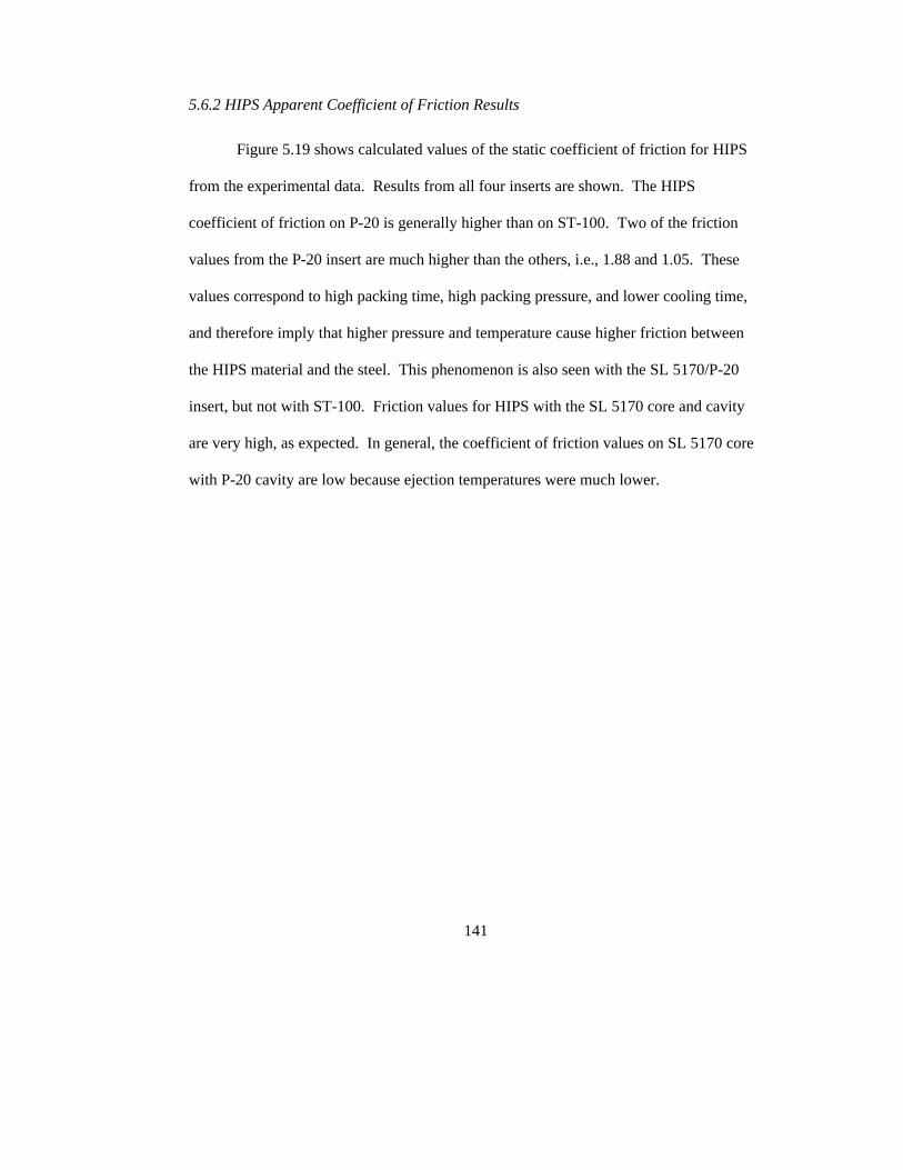
141

5.6.2 HIPS Apparent Coefficient of Friction Results

Figure 5.19 shows calculated values of the static coefficient of friction for HIPS

from the experimental data. Results from all four inserts are shown. The HIPS

coefficient of friction on P-20 is generally higher than on ST-100. Two of the friction

values from the P-20 insert are much higher than the others, i.e., 1.88 and 1.05. These

values correspond to high packing time, high packing pressure, and lower cooling time,

and therefore imply that higher pressure and temperature cause higher friction between

the HIPS material and the steel. This phenomenon is also seen with the SL 5170/P-20

insert, but not with ST-100. Friction values for HIPS with the SL 5170 core and cavity

are very high, as expected. In general, the coefficient of friction values on SL 5170 core

with P-20 cavity are low because ejection temperatures were much lower.

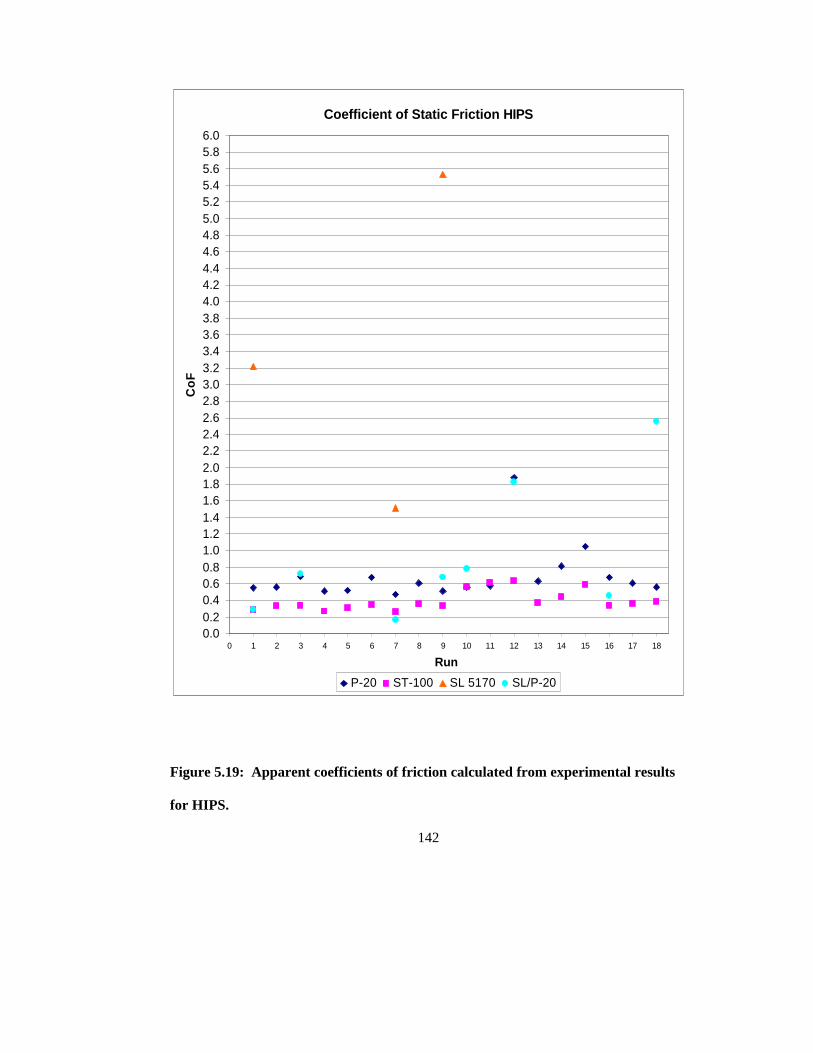
142

Coefficient of Static Friction HIPS

0.00.20.40.60.81.01.21.41.61.82.02.22.42.62.83.03.23.43.63.84.04.24.44.64.85.05.25.45.65.86.0

0 1 2 3 4 5 6 7 8 9 10 11 12 13 14 15 16 17 18

Run

Co

F

P-20 ST-100 SL 5170 SL/P-20

Figure 5.19: Apparent coefficients of friction calculated from experimental results

for HIPS.

143

5.6.3 Apparent Friction Coefficient Results from the P-20 and ST-100 Inserts

From the P-20 insert, the friction coefficient was lower for HDPE than for HIPS

for 10 out of 18 runs, most of which correspond to the higher level of packing time

(Figure 5.20). From the ST-100 insert, the friction coefficient for HDPE was higher than

for HIPS for all runs (Figure 5.21). The HDPE coefficients corresponding to low packing

time were higher than those corresponding to high packing time, whereas the HIPS

coefficients showed the opposite relation to a lesser degree.

Coefficient of Static Friction P-20

00.2

0.40.6

0.81

1.21.4

1.61.8

2

0 1 2 3 4 5 6 7 8 9 10 11 12 13 14 15 16 17 18

Run

Co

F

HDPE HIPS

Figure 5.20: Apparent coefficient of static friction for parts from the P-20 insert.

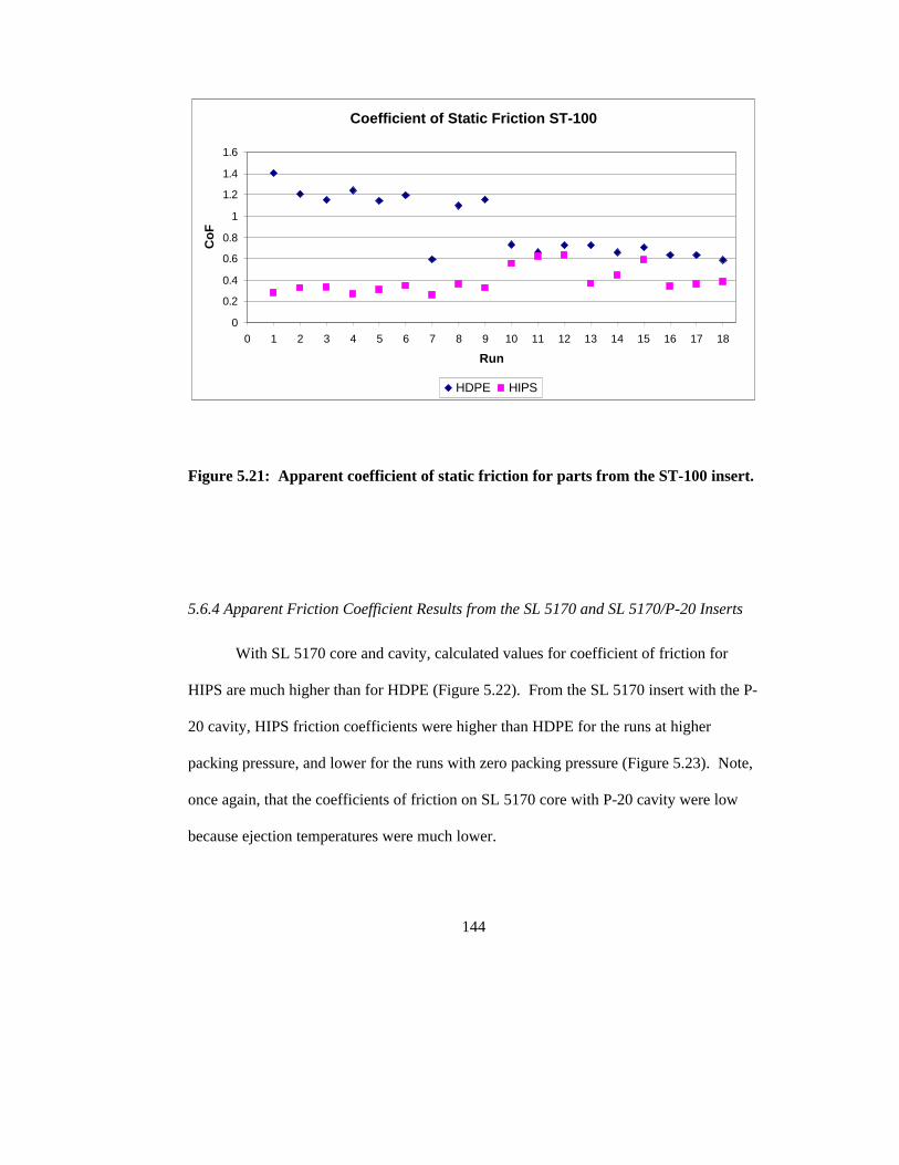
144

Coefficient of Static Friction ST-100

0

0.2

0.4

0.6

0.8

1

1.2

1.4

1.6

0 1 2 3 4 5 6 7 8 9 10 11 12 13 14 15 16 17 18

Run

Co

F

HDPE HIPS

Figure 5.21: Apparent coefficient of static friction for parts from the ST-100 insert.

5.6.4 Apparent Friction Coefficient Results from the SL 5170 and SL 5170/P-20 Inserts

With SL 5170 core and cavity, calculated values for coefficient of friction for

HIPS are much higher than for HDPE (Figure 5.22). From the SL 5170 insert with the P-

20 cavity, HIPS friction coefficients were higher than HDPE for the runs at higher

packing pressure, and lower for the runs with zero packing pressure (Figure 5.23). Note,

once again, that the coefficients of friction on SL 5170 core with P-20 cavity were low

because ejection temperatures were much lower.

145

Coefficient of Static Friction SL 5170

0.0

1.0

2.0

3.0

4.0

5.0

6.0

0 1 2 3 4 5 6 7 8 9 10 11 12 13 14 15 16 17 18

Run

Co

F

HDPE HIPS

Figure 5.22: Apparent coefficient of static friction for parts from the SL 5170

insert.

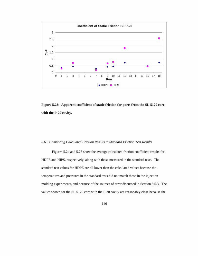
146

Coefficient of Static Friction SL/P-20

0

0.5

1

1.5

2

2.5

3

0 1 2 3 4 5 6 7 8 9 10 11 12 13 14 15 16 17 18Run

Co

F

HDPE HIPS

Figure 5.23: Apparent coefficient of static friction for parts from the SL 5170 core

with the P-20 cavity.

5.6.5 Comparing Calculated Friction Results to Standard Friction Test Results

Figures 5.24 and 5.25 show the average calculated friction coefficient results for

HDPE and HIPS, respectively, along with those measured in the standard tests. The

standard test values for HDPE are all lower than the calculated values because the

temperatures and pressures in the standard tests did not match those in the injection

molding experiments, and because of the sources of error discussed in Section 5.5.3. The

values shown for the SL 5170 core with the P-20 cavity are reasonably close because the

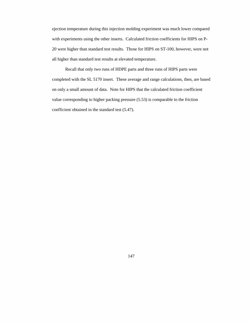
147

ejection temperature during this injection molding experiment was much lower compared

with experiments using the other inserts. Calculated friction coefficients for HIPS on P-

20 were higher than standard test results. Those for HIPS on ST-100, however, were not

all higher than standard test results at elevated temperature.

Recall that only two runs of HDPE parts and three runs of HIPS parts were

completed with the SL 5170 insert. These average and range calculations, then, are based

on only a small amount of data. Note for HIPS that the calculated friction coefficient

value corresponding to higher packing pressure (5.53) is comparable to the friction

coefficient obtained in the standard test (5.47).

148

Static Friction Coefficient for HDPE

CalculatedSTD ElevSTD RT

0.0

0.2

0.4

0.6

0.8

1.0

1.2

1.4

1.6

P-20

ST-100

SL 5170

SL/P20

Figure 5.24: Average apparent coefficient of static friction for HDPE compared to

standard test results at room temperature and elevated temperature.

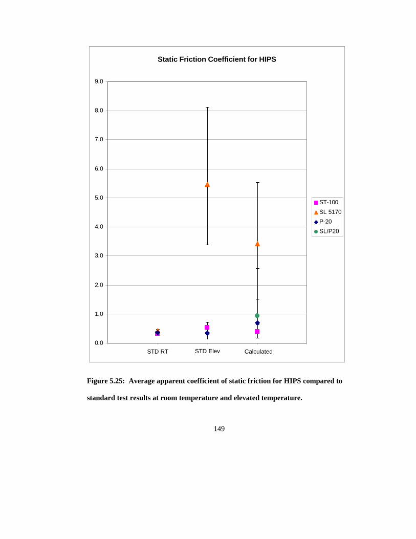
149

Static Friction Coefficient for HIPS

STD RT STD Elev Calculated0.0

1.0

2.0

3.0

4.0

5.0

6.0

7.0

8.0

9.0

ST-100

SL 5170

P-20

SL/P20

Figure 5.25: Average apparent coefficient of static friction for HIPS compared to

standard test results at room temperature and elevated temperature.

150

5.7 Other Observations of Rapid Tooled Inserts

In addition to the quantitative analyses, a number of qualitative observations were

made during experiments with the ST-100 and SL 5170 tools. These are summarized in

the paragraphs below.

The ST-100 insert seemed to operate as well as the P-20 insert. There were no

problems with core swelling or parts adhering to the sintered material. The insert held up

well for the number of parts that were processed, and had every indication that it would

last for many more. There were, however, differences in data between the ST-100 and P-

20 experiments, indicating that there are thermal and adhesion differences that affect

ejection force and friction coefficient.

The SL 5170 insert, on the other hand, operated quite differently from the other

two metal inserts, as one would expect. Surprisingly, the resin core held up for more than

105 full parts, with minimal flashing and no catastrophic failure. The following are some

of the anomalies of the SL 5170 insert discovered during processing.

It was obvious during molding of both HDPE and HIPS that there was adhesion

of the parts to the SL 5170 core (no matter which cavity was used). The adhesion was

both visible and audible. After the mold opened and before the part was ejected, the

portion of the part that adhered was more translucent than the rest. At ejection, the part

would audibly snap upon release, then slide off the core. It is quite possible that the force

from the stripper plate, in conjunction with the adhesion, forced the part to bow outward

somewhat, thus reducing the amount of shear along the core surface.

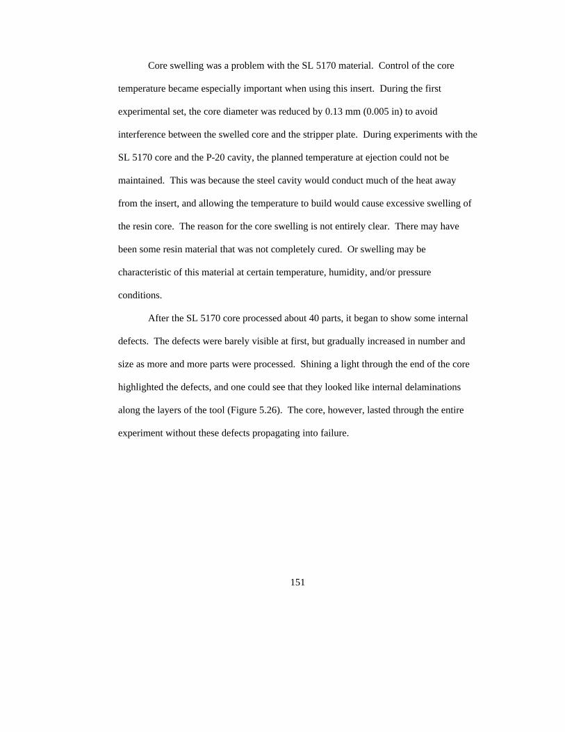
151

Core swelling was a problem with the SL 5170 material. Control of the core

temperature became especially important when using this insert. During the first

experimental set, the core diameter was reduced by 0.13 mm (0.005 in) to avoid

interference between the swelled core and the stripper plate. During experiments with the

SL 5170 core and the P-20 cavity, the planned temperature at ejection could not be

maintained. This was because the steel cavity would conduct much of the heat away

from the insert, and allowing the temperature to build would cause excessive swelling of

the resin core. The reason for the core swelling is not entirely clear. There may have

been some resin material that was not completely cured. Or swelling may be

characteristic of this material at certain temperature, humidity, and/or pressure

conditions.

After the SL 5170 core processed about 40 parts, it began to show some internal

defects. The defects were barely visible at first, but gradually increased in number and

size as more and more parts were processed. Shining a light through the end of the core

highlighted the defects, and one could see that they looked like internal delaminations

along the layers of the tool (Figure 5.26). The core, however, lasted through the entire

experiment without these defects propagating into failure.

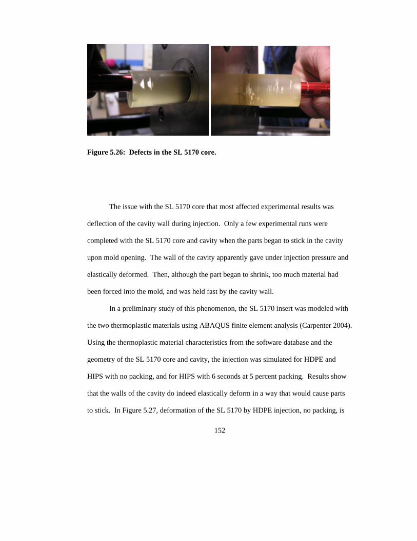
152

Figure 5.26: Defects in the SL 5170 core.

The issue with the SL 5170 core that most affected experimental results was

deflection of the cavity wall during injection. Only a few experimental runs were

completed with the SL 5170 core and cavity when the parts began to stick in the cavity

upon mold opening. The wall of the cavity apparently gave under injection pressure and

elastically deformed. Then, although the part began to shrink, too much material had

been forced into the mold, and was held fast by the cavity wall.

In a preliminary study of this phenomenon, the SL 5170 insert was modeled with

the two thermoplastic materials using ABAQUS finite element analysis (Carpenter 2004).

Using the thermoplastic material characteristics from the software database and the

geometry of the SL 5170 core and cavity, the injection was simulated for HDPE and

HIPS with no packing, and for HIPS with 6 seconds at 5 percent packing. Results show

that the walls of the cavity do indeed elastically deform in a way that would cause parts

to stick. In Figure 5.27, deformation of the SL 5170 by HDPE injection, no packing, is

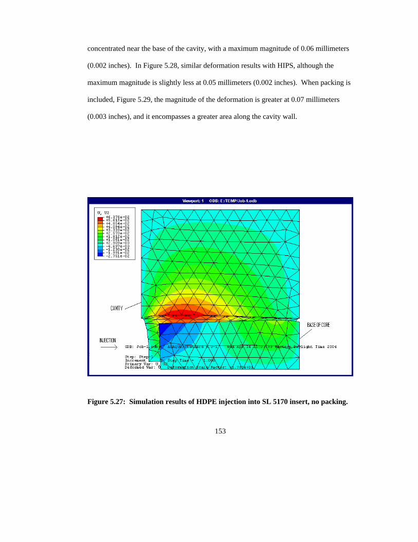
153

concentrated near the base of the cavity, with a maximum magnitude of 0.06 millimeters

(0.002 inches). In Figure 5.28, similar deformation results with HIPS, although the

maximum magnitude is slightly less at 0.05 millimeters (0.002 inches). When packing is

included, Figure 5.29, the magnitude of the deformation is greater at 0.07 millimeters

(0.003 inches), and it encompasses a greater area along the cavity wall.

Figure 5.27: Simulation results of HDPE injection into SL 5170 insert, no packing.

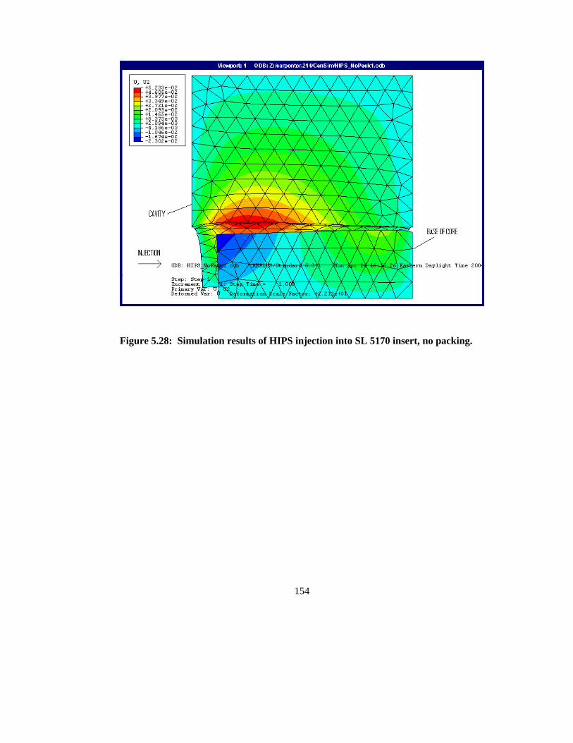
154

Figure 5.28: Simulation results of HIPS injection into SL 5170 insert, no packing.

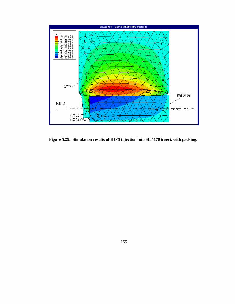
155

Figure 5.29: Simulation results of HIPS injection into SL 5170 insert, with packing.

156

CHAPTER 6

CONCLUSIONS

This chapter presents the conclusions of this research project. First, conclusions

regarding the molding of HDPE and HIPS parts using the rapid tooled inserts are

presented, including the benefits and limitations of rapid tooled injection mold inserts.

Next, the use of a model for determining ejection force and the coefficient of friction is

discussed. Implications and future work are also included, and the chapter concludes

with an overall summary.

6.1 Molding HDPE and HIPS with ST-100 and SL 5170 Inserts

6.1.1 Benefits and Limitations of Using Rapid Tooled Injection Mold Inserts

The general benefits of rapid tools were discussed in Chapter 1. These include

the ability to build complex geometries and incorporate conformal cooling lines, and

potential savings in lead times and material and labor costs. As an injection molding

insert, the ST-100 tool was very capable. Few process problems were experienced in this

157

work. This particular insert withstood the processing of 288 parts plus many test parts

with no signs of wear or damage. For these quantities, the ST-100 performed just as well

as the P-20, and even showed some advantages for processing HIPS in terms of friction

coefficients. For the scope of this work, no limitations of the ST-100 insert are noted.

The SL 5170 tool shares the same general benefits as the ST-100 and other rapid

tools as mentioned above. Some unexpected benefits, as seen in this work, include its

ability to mold both HDPE and HIPS, and durability of the core for processing more than

105 parts. The use of SL 5170 for injection molds, however, is limited because of the

deformation that occurs with high pressure and swelling of the material at high

temperature. Although the SL 5170 core did not fail catastrophically during these

experiments, it is assumed that the fatigue life of the core is limited because of the defects

that developed after approximately 40 parts. The interaction of the surface of SL 5170

with those of some thermoplastic materials, such as HIPS, is also a drawback. Adhesion

often occurs between the two surfaces, which can accelerate failure of the core and

potentially affect the quality of the part.

The statistical analysis shows the effects of processing parameters on ejection

forces for all three inserts. Packing time, cooling time, and packing pressure affect

ejection force differently between the baseline steel and the rapid tooled inserts. Effects

are also different between thermoplastic materials. Conclusions from the statistical

analysis that relate directly to the insert material are as follows:

• Ejection force increases with packing time for the SL 5170 insert.

158

• Ejection force decreases with packing time for the ST-100 insert.

• Ejection force decreases with cooling time for the P-20 insert; but this is a non-

linear effect.

6.1.2 Friction and Ejection Force Considerations

In the standard tests, the friction coefficients of HDPE were similar on P-20, ST-

100, and SL 5170 at all temperature conditions. HIPS showed a different friction

response than HDPE, and its friction coefficients varied significantly between plate

materials in heated tests. Both polymers showed highest coefficients on SL 5170 at all

three temperature conditions. The HIPS test on SL 5170 showed the interplay of the

adhesion and deformation components of friction and how this affects the friction

coefficient.

Although the standard friction tests at elevated temperatures may have given a

more accurate estimate of the friction coefficient during ejection than those at room

temperature, they still did not exactly simulate the actual process. Additional adjustments

might be made to the temperatures and normal forces applied in the standard tests to

render the results more similar to actual molding conditions.

In the injection molding experiments, ejection forces for parts from the ST-100

core were generally similar to those from the P-20 baseline core (170 – 200 N for HDPE

and 340 – 430 N for HIPS). HDPE parts from the SL 5170 core had slightly higher

ejection forces (190 to 240 N), and those from the SL 5170 core with the P-20 cavity

were higher still (250 – 330 N). Conversely, HIPS parts had higher ejection forces from

159

the SL 5170 core with the P-20 cavity (600 – 950 N), and much higher ejection forces

from the SL 5170 core (1100 – 1600 N). This seems to indicate that, when ejecting

HPDE parts from the SL 5170 core, a lower ejection temperature will increase shrinkage

and increase ejection force, and, when ejecting HIPS parts from the SL 5170 core, a

higher ejection temperature will increase adhesion and increase ejection force.

Given the discussion above and all the results of this research, the following

conclusions are drawn:

§ ST-100 inserts can be used to mold HDPE parts. This insert material performed

similarly to P-20, but was affected differently by process parameters.

Calculations of apparent coefficient of static friction indicated that friction can be

high when packing time is low, but these values did not cause extremely large

ejection forces.

§ ST-100 inserts can be used to mold HIPS parts. Once again, ST-100 performed

similarly to P-20, and in some cases had lower ejection forces.

§ SL 5170 can be used to mold HDPE parts, but with adjusted process parameters

or alternative cavity materials to minimize cavity deformation. Ejection

temperatures should be relatively high to minimize the load on the core.

Minimizing this load may extend core life prior to defect formation.

160

§ SL 5170 is not recommended for molding HIPS due to adhesion and very high

ejection forces. The coefficient of friction will increase with higher ejection

temperatures and packing times due to adhesion, which is enhanced by the

secondary forces between the two materials. Maintaining a lower ejection

temperature (e.g., by using a P-20 core) reduces the ejection force somewhat.

Core life, however, will probably be minimal.

6.2 Using a Model to Determine Ejection Force and the Coefficient of Friction

In this work the Menges model was used to determine ejection force for

comparison to experimental measurements. This model requires values for the

coefficient of static friction between the part and the core, the elastic modulus of the part

material at the time of ejection, and the relative change in diameter of the part

immediately after ejection. Each of these values is difficult to obtain and introduces error

into the calculation. The differences between the calculated ejection force and the actual

ejection force varied from 16 percent to 70 percent for HDPE, and from 44 percent to 924

percent for HIPS. While some of the calculations provided good ballpark estimates,

others did not, and only one was within 20 percent.

The static friction coefficient measurement may have been the largest contributor

to the lack of accuracy in the ejection force calculations. Standard friction tests provided

values for static friction coefficients that were an improvement over room temperature

161

values, but were still not an exact simulation of the injection molding experiment. More

standard testing at a wider range of temperature and pressure environments would be

required to determine more accurate values for the static friction coefficient that occur

during ejection of an injection molded part.

The Menges model was also used to determine the apparent coefficient of friction

for comparison to results from the standard friction tests. The specific description of

friction coefficient is still largely a mystery. The term includes deformation and adhesion

in unknown proportions and affected by certain conditions to unknown extents. The

calculation of apparent coefficient of friction from ejection force models, as was done

here, results in a value that encompasses a complete surface interaction under the given

processing conditions. How this value compares with standard measures of friction

coefficient has not been entirely clear. Furthermore, the calculated value of the apparent

coefficient of friction includes error from the measurements of elastic modulus and the

relative change in diameter, and so is not an apples-to-apples comparison with the

standard friction test values.

The apparent friction coefficient calculation, however, can be potentially useful in

testing a new material for an injection mold insert application. For example, to estimate

the ejection forces that will occur, a simple cylindrical mold insert can be built with the

new material, and the apparent coefficient of friction can be calculated using the Menges

model and injection molding data from the cylindrical mold. This calculated value can

then be applied to the model to estimate ejection force for molds having different

geometries but the same materials and similar processing parameters.

162

Results from this work, however, are insufficient to validate this application of the

model. Additional experimentation with a different part geometry would be required to

provide comparison data and prove this concept.

6.3 Implications and Future Work

This work has included friction testing of thermoplastics against rapid prototyped

materials, following a standard procedure and including higher temperatures; direct

measurement of ejection force from steel and rapid tooled injection mold inserts;

calculation of ejection forces using a model developed by Menges; and determination of

the apparent coefficient of static friction from experimental data using the same Menges

model.

A good indication of the processing capability of a mold material are its ejection

force requirements. The experimental results provide these data for all material

combinations. The results were compared among thermoplastic and mold insert

materials, and then compared to calculated ejection force values. These results give an

indication of the usefulness of the ejection force model.

The static friction coefficient results from the standard tests were also compared

among materials, and then compared with calculations of apparent coefficients of

friction. The friction test data are a useful reference for understanding the basic friction

conditions between the thermoplastics, HDPE and HIPS, and the mold insert materials,

163

P-20, ST-100 and SL 5170. Friction results from the standard tests have also pointed out

the adhesion phenomenon that occurs between HIPS and SL 5170. The adhesion results

from the molecular forces between the two materials and is enhanced by higher ejection

temperatures.

The statistical results are useful for determining those process parameters that can

be adjusted to optimize ejection force for the material pairs studied. Analysis of variance

has shown which parameters affect ejection force and how strong those effects are for the

given process window. This information can be used, once a decision has been made to

use one of these inserts, to design a process that meets ejection force requirements.

The experiments have shown the molding of HDPE and HIPS parts with P-20 and

ST-100 mold inserts as rather routine. The more interesting results come from the use of

the SL 5170 insert. While HDPE parts can be molded with SL 5170 inserts, higher

friction coefficients and ejection forces will result. HIPS parts were molded with the SL

5170 insert as well, but with extremely high friction coefficients and ejection forces.

These forces caused high cyclic loads on the SL 5170 core, leading to the formation of

internal defects. Additionally, deformation of the cavity occurred during injection.

These considerations must be taken into account in the application of this rapid tooled

material for injection molds.

Overall, the data are useful for choosing mold insert materials, for deciding

whether or not to use rapid tooled inserts for small quantity production, for development

of rapid prototyping materials and processes, or for injection molding part or machine

design.

164

As mentioned in the previous section, additional work in static friction coefficient

measurement and ejection force comparison with a different part geometry would

enhance the current work. Friction testing under various temperature and pressure

conditions may provide more accurate values of the friction that exists during ejection.

These values could then be used with the ejection force model. Further injection molding

experiments with a different part shape would provide ejection force data to compare to

those from the cylindrical part. This comparison would indicate whether or not the

Menges model could be used to determine ejection forces for new mold insert materials.

Other possible areas for future work include further study on the deformation and

swelling of the SL 5170 material, failure testing and analysis of the SL 5170 core,

optimization of injection molding process parameters, and materials characterization for

adhesion. The deformation and swelling of the SL 5170 resin can be investigated to

determine their actual causes. If curing of the material is an issue, improvements in the

stereolithography process or its post-cure may have an effect. The selection of alternative

materials may also be a solution, including more recently developed materials and resins

that contain fillers. The defects that developed in the SL 5170 core can be analyzed to

confirm whether or not they are in fact delaminations and to determine why they

occurred. Improvements in the building or curing of the stereolithography tool might be

required, or it may be characteristic of the process or material. Further testing to failure

would provide useful data on the actual life expectancy of the core.

Any of the designed experiments could be expanded to encompass a broader

processing window, leading to the optimization of process parameters. This might be

165

especially useful for the SL 5170 core and the HDPE thermoplastic. Further study of the

temperature and pressure parameters would further delineate the effects of the adhesion

component of friction and clarify a feasible processing space.

Since the role of adhesion and friction in injection molding is not explicitly

understood, further study in this area would also be useful. This would include materials

characterization and research into the interfaces between the thermoplastics and rapid

prototyped materials.

Areas that were not addressed in this work include part quality, as-built rapid

tools, and conformal cooling lines. First, the performance of rapid tooled inserts cannot

be completely assessed without consideration for part quality; this would include

dimensional and surface finish quality. Second, the rapid tools used in this work were

finish machined. The advantage to using rapid tools is maximized, however, if they are

inserted as built and not post-processed. And third, the addition of conformal cooling

lines would allow more control of processing temperatures. The nature of rapid

prototyping processes is such that they facilitate the incorporation of conformal cooling

lines. Further research in each of these areas would contribute to the potential use of

rapid tools for injection molding.

6.4 Summary

The application of rapid prototyped tools for injection molding, if technically

feasible, may allow for small quantity production by reducing the cost of tooling. This

166

work has investigated one aspect of the technical feasibility through testing and

experimentation to determine ejection force requirements and coefficients of friction.

Friction coefficients between thermoplastics and rapid tooled materials were measured

using a modified standard testing process. Injection molding experiments were

conducted using three mold insert materials, P-20 steel, laser sintered ST-100, and

stereolithography SL 5170 resin. Ejection forces for cylindrical parts molded with high

density polyethylene and high impact polystyrene were measured directly and then

compared with values calculated from an ejection force model. Process parameters

affected the adhesion and deformation components of friction differently, depending on

the materials characteristics. Results show that ST-100 is a good candidate for injection

molding tools, and that SL 5170 may be a good candidate for molding some

thermoplastics, but only in very small quantities.

167

LIST OF REFERENCES

Anderson, D. M., Pine, B. J. II 1997, Agile Product Development for Mass Customization, Irwin Professional Publishing, Chicago.

ASM International 1992, “Static and Kinetic Friction Coefficients for Selected Materials,” ASM Handbook, vol. 18, p. 73.

Balsamo, R., Hayward, D., Malloy, R. 1993, “An Experimental Evaluation of Ejection Forces: Frictional Effects,” ANTEC, pp. 2515-2521.

Beaman, J.J., Barlow, J.W., Bourell, D.L., Crawford, R.H., Marcus, H.L., McAlea, K.P 1997, Solid Freeform Fabrication: A new Direction in Manufacturing, Kluwer Academic Publishers, Dordrecht.

Beer, F.P., Johnston, E.R. 1981, Mechanics of Materials, McGraw-Hill, New York, pp 325-6.

Benabdallah, H., Fisa, B. 1989, “Static Friction Coefficient of Some Thermoplastics,” ANTEC, pp. 1055-1058.

Benabdallah, S.H. 1993, “Static Shear Strength and Adhesion Friction of Some Thermoplastics,” Polymer Engineering and Science, vol. 33, no. 9, pp. 543-548.

Bourell, D.L., Crawford, R.H., Marcus, H.L., Beaman, J.J., Barlow, J.W. 1994, “Selective Laser Sintering of Metals,” Proceedings of the 1994 ASME Winter Annual Meeting, November, pp. 519-528.

Briscoe, B.J. 1981, “Wear of polymers: an essay on fundamental aspects,” Tribology International, August, pp. 231-243.

Brydson, J.A. 1999, Plastics Materials, Butterworth-Heinemann, [On line] Available from www.knovel.com, [June 2004].

Burke, C.T. 1991, Ejection Force Measurement for the Injection Molding Process, Master Thesis, University of Lowell, Appendix E.

168

Burke, C., Malloy, R. 1991, “An Experimental Study of the Ejection Forces Encountered During Injection Molding,” ANTEC 1991, pp. 1781-1787.

Cagle, C.V. (ed.) 1973, Handbook of Adhesive Bonding, McGraw-Hill, New York.

Callister, W.D., Jr. 1985, Materials Science and Engineering An Introduction, John Wiley & Sons, New York.

Campbell, C. 2000, “Rapid Tooling for Real World Applications,” Rapid Tooling Technologies for Plastic Applications, Society of Manufacturing Engineers Symposium, October, Detroit, MI.

Carpenter, B. 2004, personal communication.

Castle Island, “Worldwide Guide to Rapid Prototyping,” [Online]. Copyright Castle Island Co. Available: home.att.net/~castleisland/home.htm [May 2003].

Cedorge, T., Colton, J. 2000, “Draft Angle and Surface Roughness Effects on Stereolithography Molds,” Polymer Engineering and Science, vol. 40, no. 7, pp. 1581-1588.

Cho, W., Sachs, E. M., Patrikalakis, N., M. 2001, “Solid Freeform Fabrication with Local Composition Control,” Rapid Prototyping, Society of Manufacturing Engineers, vol. 7, no. 2, pp 1-5.

Colton, J. S., Crawford, J., Pham, G., Rodet, V. 2001, “Failure of Rapid Prototype Molds During Injection Molding,” CIRP Annals – Manufacturing Technology, vol. 50, no. 1, pp. 129-132.

Colton, J.S., LeBaut, Y. 2000, “Thermal Effects on Stereolithography Injection Mold Inserts,” Polymer Engineering and Science, vol. 40, no. 6.

Czichos, H. 1983, “Influence of Adhesive and Abrasive Mechanisms on the Tribological Behaviour of Thermoplastic Polymers,” Wear, vol. 88, pp. 27-43.

Czichos, H. 1985, “Contact Deformation and Static Friction of Polymers, Influences of Viscoelasticity and Adhesion,” Polymer Wear and Its Control, American Chemical Society, pp. 3-26.

Dalgarno, K. W., Stewart, T. D. 2001, “Manufacture of production injection mould tooling incorporating conformal cooling channels via indirect selective laser sintering,” Proceedings of the Institution of Mechanical Engineers Part B, Journal of Engineering Manufacture, vol. 215, pp.1323-1332.

Dearnley, P.A. 1999, “Low friction surfaces for plastic injection moulding dies – an experimental case study,” Wear, vol. 225-229, pp. 1109-1113.

169

Dickens, P., Rudgley, M. 2001, “DirectAIMTM in a New Direction,” Rapid Prototyping and Manufacturing Conference [CD-ROM], Society of Manufacturing Engineers, Cincinnati.

Eley, D.D. (ed.) 1961, Adhesion, Oxford University Press, London.

Ferreira, E.C., Neves, N.M., Muschalle, R., Pouzada, A.S. 2001, “Friction Properties of Thermoplastics in Injection Molding,” ANTEC Portugal, [Online]. Available: www.dep.uminho.pt/NP/2001_03.pdf, [July 2003].

Ferreira, E. C., Muschalle, R., Neves, N. M., Pouzada, A. S. 2002, “Analysis of parameters determining the friction properties of thermoplastics in injection molding,” ANTEC 2002, vol. 1, pp. 878-881.

Glanvill, A.B. 1971, The Plastics Engineer’s Data Book, Machinery Publishing Co. Ltd., The Whitefriars Press Ltd., London, p. 30.

Harris, R. A., Dickens, P. M. 2001, “Mould Variables in Stereolithography Injection Moulds,” ANTEC 2001, vol. 1, pp 107-111.

Harris, R. A., Dickens, P. M. 2003, “Determining, Understanding, and Controlling the Morphology of Injection Moulded Parts Produced in Stereolithography Moulds,” ANTEC 2003, pp. 889-893.

Hopkinson, N., Dickens, P. 1999, “Study of ejection forces in the AIM™ process,” Materials and Design, vol. 20, pp. 99-105.

Hopkinson, N., Dickens, P. 2000a, “Conformal Cooling and Heating Channels using Laser Sintered Tools,” Proceedings of the Solid Freeform Fabrication Symposium, Austin, TX, pp. 490-497.

Hopkinson, N., Dickens, P. 2000b, “A comparison between stereolithography and aluminium injection moulding tools,” Rapid Prototyping Journal, vol. 6, no.4, pp. 253-258.

Hopkinson, N., Dickens, P. 2000c, “Predicting stereolithography injection mould tool behaviour using models to predict ejection force and tool strength,” International Journal of Production Research, vol. 38, no. 16, pp. 3747-3757.

Hopkinson, N., Dickens, P. 2000d, “Using stereolithography tools for injection moulding: research into tensile tool failure and unexpected benefits of the process,” Proceedings of the Institution of Mechanical Engineers, vol. 214, part B, pp. 891-899.

Jacobs, P. F. 1996, Stereolithography and other RP&M Technologies, Society of Manufacturing Engineers, Dearborn, MI, ASME Press, New York.

170

Jansen, K.M.B, Titomanlio, G. 1996, “Effect of Pressure History on Shrinkage and Residual Stresses – Injection Molding with Constrained Shrinkage,” Polymer Engineering and Science, vol. 36, no. 15, pp 2029-2040.

Kabanemi, K.K., Vaillancourt, Wang, H., Salloum, G. 1998, “Residual Stresses, Shrinkage and Warpage of Complex Injection Molded Products: Numerical Simulation and Experimental Validation,” Polymer Engineering and Science, vol. 38, no. 1, pp. 21-37.

Kai, C.C., Fai, L.K 1997, Rapid Prototyping, Principles and Applications in Manufacturing, John Wiley & Sons, New York.

Kaminsky, P.G. 1996, “Lean Logistics: Better, Faster, Cheaper,” Defense Issues, vol. 11, no. 99, [Online] Available: http://www.defenselink.mil/speeches/index.html.

Karapatis, N.P., van Griethuysen, J.-P.S., Glardon, R. 1998, “Direct rapid tooling: a review of current research,” Rapid Prototyping Journal, vol. 4, no. 2, pp. 77-89.

Keicher, D., Gorman, P., Taute, L. 2001, “A Novel Method for Fabrication and Repair of Tooling?” National Tooling and Machining Association Record, January.

Kinsella, M.E. 2000, “Piloted Concepts for Commercial-Military Integration Ready for Implementation,” Program Manager, July-August, p. 30.

Li, Y., Gargiulo, E.P., Keefe, M. 2000, “Studies in Direct Tooling Using Stereolithography,” Journal of Manufacturing Science and Engineering, vol. 122, May, pp. 316-322.

Malloy, R., Majeski, P. 1989, “Design of Pin Ejector Systems for Injection Molds,” ANTEC 1989, pp. 1231-1235.

MatWeb Material Property Data (March 2004), [Online], Available from: www.matweb.com [6 June 2004].

McAlea, K., Booth, R., Forderhase, P., Lakshminarayan, U. 1995, “Materials for Selective Laser Sintering Processing,” Proceedings of the 27th International SAMPE Technical Conference, vol. 27, pp. 949-961.

Menges, G., Bangert, H. 1981, “Measurement of Coefficients of Static Friction as a Means of Determining Opening and Demoulding Forces in Injection Moulds,” Kunststoffe, vol. 71, no. 9, pp. 552-557.

Menges, G., Michaeli, W., Mohren, P. 2001, How to Make Injection Molds, Hanser Gardner Publications, Munich, Cincinnati.

171

Michaeli, W., Gutberlet, D., Hoffmann, S., Zachert, J. 1999, “Development steps for integrated material modeling for a semicrystalline polymer,” Computational Materials Science, vol.16, pp. 151-157.

Michalski, D.D. 2000, A Parametric Study of the Ejection Forces Encountered During the Injection-Molding Process, Master Thesis, The Ohio State University.

Muschalle, R. 2001, “Friction Behaviour of Thermoplastics,” Kunststoffe, vol. 91, no. 12, pp. 48-54.

Nelson, C., Kepler, J., Booth, R., Conner, P. 1998, “Direct Injection Molding Tooling Inserts from the SLS Process with Copper Polyamide,” Proceedings of the Solid Freeform Fabrication Symposium, August, Austin TX, pp. 451-459.

Optomec, Inc. 2001, company literature, Albuquerque.

Osswald, T.A. 1998, Polymer Processing Fundamentals, Hanser Publishers, Munich.

Palmer, A.E., Colton, J.S., 2000, “Failure Mechanisms in Stereolithography Injection Molding Tooling,” Polymer Engineering and Science, vol. 40, no. 6, pp. 1395-1404.

Pantani, R., Titomanlio, G. 1999, “Analysis of Shrinkage Development of Injection Moulded PS Samples,” Intern. Polymer Processing, vol. XIV, no.2, pp. 183-190.

Petrie, E.M. 2000, Handbook of Adhesives and Sealants, McGraw-Hill, [On line] Available from www.knovel.com, [June 2004].

Pham, G.T., Colton, J.S. 2002, “Ejection Force Modeling for Stereolithography Injection Molding Tools,” Polymer Engineering and Science, vol. 42, no. 4, pp.681-693.

Pham, D. T., Dimov, S. S., Lacan, F. 2000, “The RapidTool process: technical capabilities and applications,” Proceedings of the Institution of Mechanical Engineers Part B, Journal of Engineering Manufacture,vol. 214, pp 107-116.

Pine, B. J. II 1993, Mass Customization – The new Frontier in Business Competition, Harvard Business School Press, Boston.

Pontes, A.J., Pinho, A.M., Miranda, A.S., Pouzada, A.S. 1997, “Effect of Processing Conditions on Ejection Forces in Injection Moulds,” O Molde, October-December, pp. 25-34.

Pontes, A.J., Pantani, R., Titomanlio, G., Pouzada, A.S. 2001, “Prediction of Ejection Forces in Tubular Moldings in Amorphous Polymers,” ANTEC, vol. I, pp. 927-931.

172

Pontes, A.J., Brito, A.M., and Pouzada, A.S. 2002, “Assessment of the Ejection Force in Tubular Injection Moldings,” Journal of Injection Molding Technology, vol. 6, no. 4, pp. 343-352.

Popov, E.P. 1976, Mechanics of Materials, second edition, Prentice-Hall, Inc., Englewood Cliffs, New Jersey.

Rosato, D.V., Rosato, D.V. 1986, Injection Molding Handbook, Van Nostrand Reinhold Company, New York.

Rubin, I.I. (ed.) 1990, Handbook of Plastic Materials and Technology, John Wiley & Sons, Inc., New York.

Sachs, E., Wylonis, E., Allen, S., Cima, M., Guo H. 2000, “Production of Injection Molding Tooling With Conformal Cooling Channels Using the Three Dimensional Printing Process,” Polymer Engineering and Science, May, vol. 40, no. 5, pp. 1232-1247.

Sasaki, T., Koga, N., Shirai, K., Koayashi, Y., Toyoshima, A. 2000, “An experimental study on ejection forces of injection molding,” Precision Engineering, vol. 24, pp. 270-273.

Shen, K., Chen, L.-M., Jiang, L. 1999, “Calculation of ejection force of hollow, thin walled, and injection molded cones,” Plastics, Rubber, and Composites, vol. 28, no. 7, pp. 341-345.

Titomanlio, G., Jansen, K.M.B. 1996, “In-Mold Shrinkage and Stress Prediction in Injection Molding,” Polymer Engineering and Science, vol. 36, no. 15, pp. 2041-2049.

Trantina, G.G., Nimmer, R. 1994, Structural Analysis of Thermoplastic Components, McGraw-Hill, NewYork.

University of Southern Mississippi, “The Macrogalleria,” [Online]. Copyright 1995-2002 by the Department of Polymer Science, Available: www.psrc.usm.edu/macrog/index.htm [November 2003].

Victor, B., Boynton, A. 1998, Invented Here – Maximizing Your Organization’s Internal Growth and Profitability, Harvard Business School Press, Boston.

Wang, H., Kabanemi, K. K., Salloum, G. 1997

Wang, H., Kabanemi, K. K., Salloum, G. 2000, “Numerical and Experimental Studies on the Ejection of Injection-Molded Plastic Products,” Polymer Engineering and Science, vol. 40, no. 3, pp. 826-840.

173

Weaver, T.J., Thomas, J.A., Atre, S.V., German, R.M. 2000, “Time compression-rapid steel tooling for an ever-changing world,” Materials and Design, vol. 21, pp. 409-415.

Wu, S. 1982, Polymer Interface and Adhesion, Marcel Dekker, New York.

Wypych, G. 2004, Handbook of Plasticizers, Noyes Publications, [On line] Available from www.knovel.com, [June 2004].

174

APPENDIX A

DATA TABLES

175

Figure A.1: Sample plots from tensile test data.

HDPE at Temperature - Sample

0

50

100

150

200

250

-0.05 0 0.05 0.1 0.15 0.2 0.25 0.3

Extension i/i

Lo

ad lb

s

60 C

50 C

40 C

30 C

RT

HIPS at Temperature - Sample

0

50

100

150

200

250

300

350

400

0 0.05 0.1 0.15 0.2

Elongation i/i

Load

lbs

Room Temp

30 C

40 C

50 C

60 C

Type I Specimen - HDPEThickness 3.09 mm 0.12 in

Width 12.35 mm 0.49 inArea 38.22 mm2 0.06 in2

Type I Specimen - HIPSThickness 3.12 mm 0.12 in

Width 12.76 mm 0.50 inArea 39.85 mm2 0.06 in2

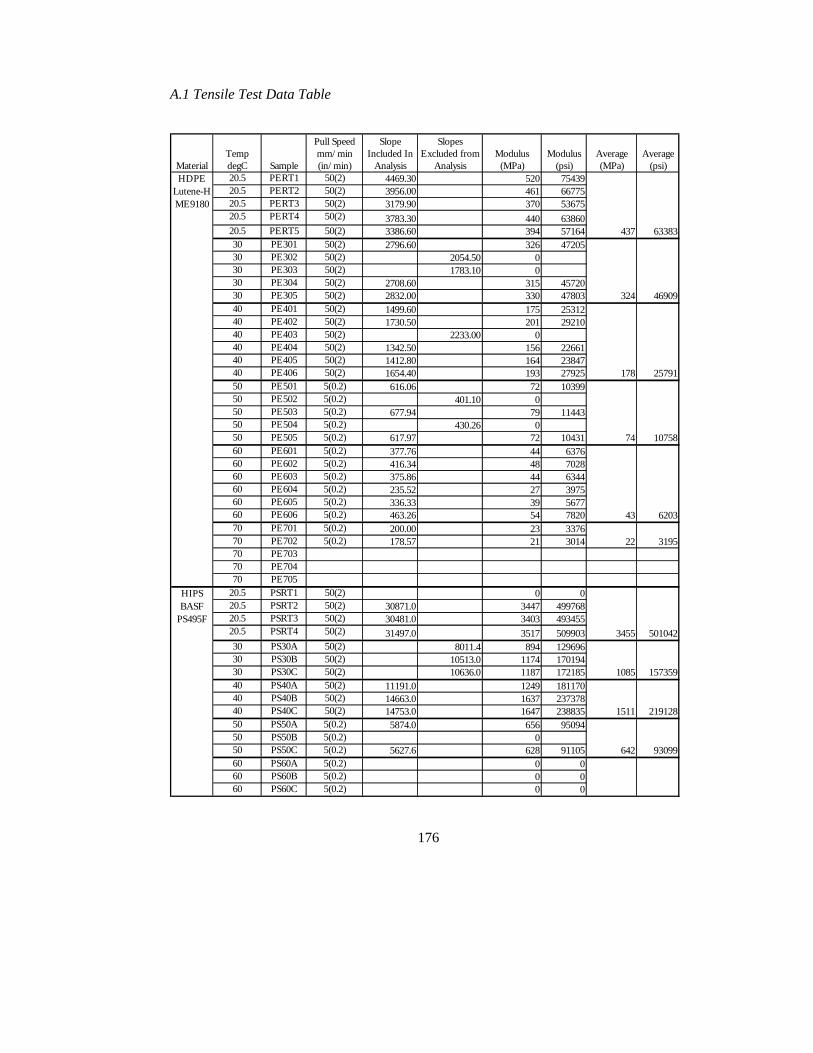
176

A.1 Tensile Test Data Table

MaterialTemp degC Sample

Pull Speedmm/min (in/min)

Slope Included In

Analysis

Slopes Excluded from

AnalysisModulus

(MPa)Modulus

(psi)Average (MPa)

Average (psi)

HDPE 20.5 PERT1 50(2) 4469.30 520 75439Lutene-H 20.5 PERT2 50(2) 3956.00 461 66775ME9180 20.5 PERT3 50(2) 3179.90 370 53675

20.5 PERT4 50(2) 3783.30 440 6386020.5 PERT5 50(2) 3386.60 394 57164 437 6338330 PE301 50(2) 2796.60 326 4720530 PE302 50(2) 2054.50 030 PE303 50(2) 1783.10 030 PE304 50(2) 2708.60 315 4572030 PE305 50(2) 2832.00 330 47803 324 4690940 PE401 50(2) 1499.60 175 2531240 PE402 50(2) 1730.50 201 2921040 PE403 50(2) 2233.00 040 PE404 50(2) 1342.50 156 2266140 PE405 50(2) 1412.80 164 2384740 PE406 50(2) 1654.40 193 27925 178 2579150 PE501 5(0.2) 616.06 72 1039950 PE502 5(0.2) 401.10 050 PE503 5(0.2) 677.94 79 1144350 PE504 5(0.2) 430.26 050 PE505 5(0.2) 617.97 72 10431 74 1075860 PE601 5(0.2) 377.76 44 637660 PE602 5(0.2) 416.34 48 702860 PE603 5(0.2) 375.86 44 634460 PE604 5(0.2) 235.52 27 397560 PE605 5(0.2) 336.33 39 567760 PE606 5(0.2) 463.26 54 7820 43 620370 PE701 5(0.2) 200.00 23 337670 PE702 5(0.2) 178.57 21 3014 22 319570 PE70370 PE70470 PE705

HIPS 20.5 PSRT1 50(2) 0 0BASF 20.5 PSRT2 50(2) 30871.0 3447 499768

PS495F 20.5 PSRT3 50(2) 30481.0 3403 49345520.5 PSRT4 50(2) 31497.0 3517 509903 3455 50104230 PS30A 50(2) 8011.4 894 12969630 PS30B 50(2) 10513.0 1174 17019430 PS30C 50(2) 10636.0 1187 172185 1085 15735940 PS40A 50(2) 11191.0 1249 18117040 PS40B 50(2) 14663.0 1637 23737840 PS40C 50(2) 14753.0 1647 238835 1511 21912850 PS50A 5(0.2) 5874.0 656 9509450 PS50B 5(0.2) 050 PS50C 5(0.2) 5627.6 628 91105 642 9309960 PS60A 5(0.2) 0 060 PS60B 5(0.2) 0 060 PS60C 5(0.2) 0 0

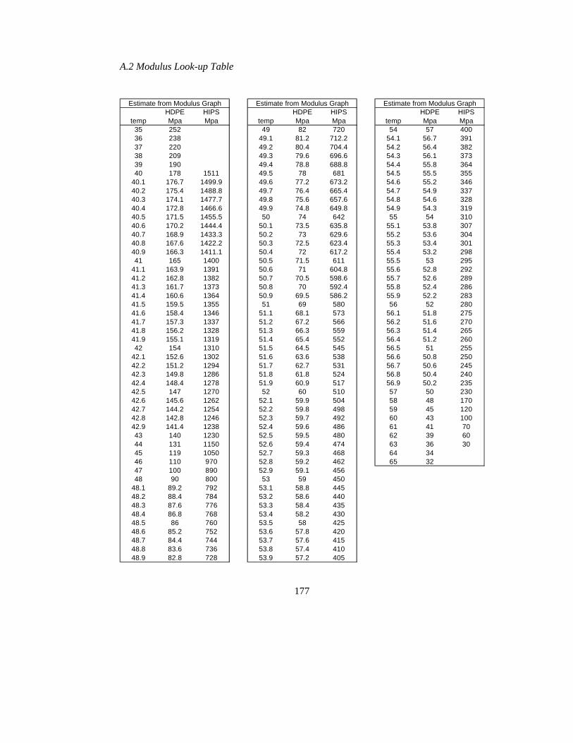
177

A.2 Modulus Look-up Table

Estimate from Modulus Graph Estimate from Modulus Graph Estimate from Modulus GraphHDPE HIPS HDPE HIPS HDPE HIPS

temp Mpa Mpa temp Mpa Mpa temp Mpa Mpa35 252 49 82 720 54 57 40036 238 49.1 81.2 712.2 54.1 56.7 39137 220 49.2 80.4 704.4 54.2 56.4 38238 209 49.3 79.6 696.6 54.3 56.1 37339 190 49.4 78.8 688.8 54.4 55.8 36440 178 1511 49.5 78 681 54.5 55.5 355

40.1 176.7 1499.9 49.6 77.2 673.2 54.6 55.2 34640.2 175.4 1488.8 49.7 76.4 665.4 54.7 54.9 33740.3 174.1 1477.7 49.8 75.6 657.6 54.8 54.6 32840.4 172.8 1466.6 49.9 74.8 649.8 54.9 54.3 31940.5 171.5 1455.5 50 74 642 55 54 31040.6 170.2 1444.4 50.1 73.5 635.8 55.1 53.8 30740.7 168.9 1433.3 50.2 73 629.6 55.2 53.6 30440.8 167.6 1422.2 50.3 72.5 623.4 55.3 53.4 30140.9 166.3 1411.1 50.4 72 617.2 55.4 53.2 29841 165 1400 50.5 71.5 611 55.5 53 295

41.1 163.9 1391 50.6 71 604.8 55.6 52.8 29241.2 162.8 1382 50.7 70.5 598.6 55.7 52.6 28941.3 161.7 1373 50.8 70 592.4 55.8 52.4 28641.4 160.6 1364 50.9 69.5 586.2 55.9 52.2 28341.5 159.5 1355 51 69 580 56 52 28041.6 158.4 1346 51.1 68.1 573 56.1 51.8 27541.7 157.3 1337 51.2 67.2 566 56.2 51.6 27041.8 156.2 1328 51.3 66.3 559 56.3 51.4 26541.9 155.1 1319 51.4 65.4 552 56.4 51.2 26042 154 1310 51.5 64.5 545 56.5 51 255

42.1 152.6 1302 51.6 63.6 538 56.6 50.8 25042.2 151.2 1294 51.7 62.7 531 56.7 50.6 24542.3 149.8 1286 51.8 61.8 524 56.8 50.4 24042.4 148.4 1278 51.9 60.9 517 56.9 50.2 23542.5 147 1270 52 60 510 57 50 23042.6 145.6 1262 52.1 59.9 504 58 48 17042.7 144.2 1254 52.2 59.8 498 59 45 12042.8 142.8 1246 52.3 59.7 492 60 43 10042.9 141.4 1238 52.4 59.6 486 61 41 7043 140 1230 52.5 59.5 480 62 39 6044 131 1150 52.6 59.4 474 63 36 3045 119 1050 52.7 59.3 468 64 3446 110 970 52.8 59.2 462 65 3247 100 890 52.9 59.1 45648 90 800 53 59 450

48.1 89.2 792 53.1 58.8 44548.2 88.4 784 53.2 58.6 44048.3 87.6 776 53.3 58.4 43548.4 86.8 768 53.4 58.2 43048.5 86 760 53.5 58 42548.6 85.2 752 53.6 57.8 42048.7 84.4 744 53.7 57.6 41548.8 83.6 736 53.8 57.4 41048.9 82.8 728 53.9 57.2 405

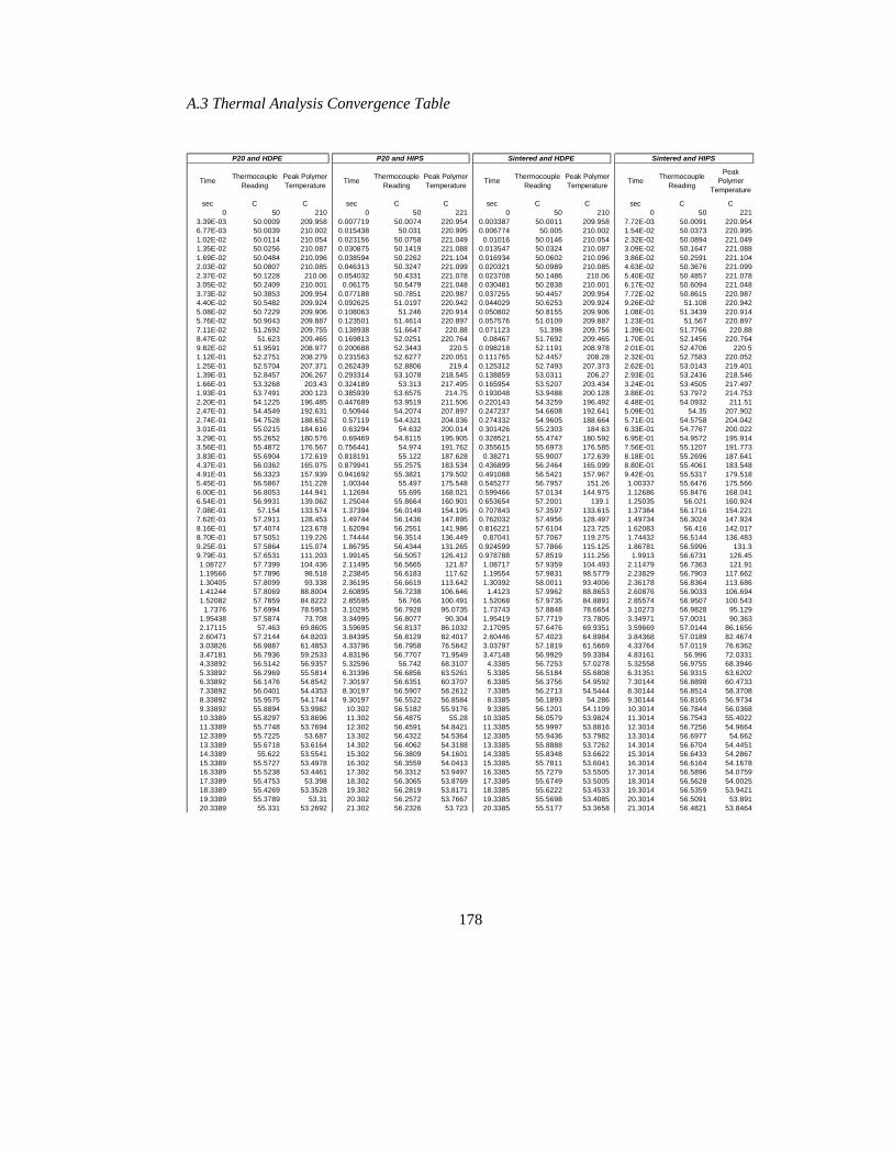
178

A.3 Thermal Analysis Convergence Table

TimeThermocouple

ReadingPeak Polymer Temperature

TimeThermocouple

ReadingPeak Polymer Temperature

TimeThermocouple

ReadingPeak Polymer Temperature

TimeThermocouple

Reading

Peak Polymer

Temperature

sec C C sec C C sec C C sec C C0 50 210 0 50 221 0 50 210 0 50 221

3.39E-03 50.0009 209.958 0.007719 50.0074 220.954 0.003387 50.0011 209.958 7.72E-03 50.0091 220.9546.77E-03 50.0039 210.002 0.015438 50.031 220.995 0.006774 50.005 210.002 1.54E-02 50.0373 220.9951.02E-02 50.0114 210.054 0.023156 50.0758 221.049 0.01016 50.0146 210.054 2.32E-02 50.0894 221.0491.35E-02 50.0256 210.087 0.030875 50.1419 221.088 0.013547 50.0324 210.087 3.09E-02 50.1647 221.0881.69E-02 50.0484 210.096 0.038594 50.2262 221.104 0.016934 50.0602 210.096 3.86E-02 50.2591 221.1042.03E-02 50.0807 210.085 0.046313 50.3247 221.099 0.020321 50.0989 210.085 4.63E-02 50.3676 221.0992.37E-02 50.1228 210.06 0.054032 50.4331 221.078 0.023708 50.1486 210.06 5.40E-02 50.4857 221.0783.05E-02 50.2409 210.001 0.06175 50.5479 221.048 0.030481 50.2838 210.001 6.17E-02 50.6094 221.0483.73E-02 50.3853 209.954 0.077188 50.7851 220.987 0.037255 50.4457 209.954 7.72E-02 50.8615 220.9874.40E-02 50.5482 209.924 0.092625 51.0197 220.942 0.044029 50.6253 209.924 9.26E-02 51.108 220.9425.08E-02 50.7229 209.906 0.108063 51.246 220.914 0.050802 50.8155 209.906 1.08E-01 51.3439 220.9145.76E-02 50.9043 209.887 0.123501 51.4614 220.897 0.057576 51.0109 209.887 1.23E-01 51.567 220.8977.11E-02 51.2692 209.755 0.138938 51.6647 220.88 0.071123 51.398 209.756 1.39E-01 51.7766 220.888.47E-02 51.623 209.465 0.169813 52.0251 220.764 0.08467 51.7692 209.465 1.70E-01 52.1456 220.7649.82E-02 51.9591 208.977 0.200688 52.3443 220.5 0.098218 52.1191 208.978 2.01E-01 52.4706 220.51.12E-01 52.2751 208.279 0.231563 52.6277 220.051 0.111765 52.4457 208.28 2.32E-01 52.7583 220.0521.25E-01 52.5704 207.371 0.262439 52.8806 219.4 0.125312 52.7493 207.373 2.62E-01 53.0143 219.4011.39E-01 52.8457 206.267 0.293314 53.1078 218.545 0.138859 53.0311 206.27 2.93E-01 53.2436 218.5461.66E-01 53.3268 203.43 0.324189 53.313 217.495 0.165954 53.5207 203.434 3.24E-01 53.4505 217.4971.93E-01 53.7491 200.123 0.385939 53.6575 214.75 0.193048 53.9488 200.128 3.86E-01 53.7972 214.7532.20E-01 54.1225 196.485 0.447689 53.9519 211.506 0.220143 54.3259 196.492 4.48E-01 54.0932 211.512.47E-01 54.4549 192.631 0.50944 54.2074 207.897 0.247237 54.6608 192.641 5.09E-01 54.35 207.9022.74E-01 54.7528 188.652 0.57119 54.4321 204.036 0.274332 54.9605 188.664 5.71E-01 54.5758 204.0423.01E-01 55.0215 184.616 0.63294 54.632 200.014 0.301426 55.2303 184.63 6.33E-01 54.7767 200.0223.29E-01 55.2652 180.576 0.69469 54.8115 195.905 0.328521 55.4747 180.592 6.95E-01 54.9572 195.9143.56E-01 55.4872 176.567 0.756441 54.974 191.762 0.355615 55.6973 176.585 7.56E-01 55.1207 191.7733.83E-01 55.6904 172.619 0.818191 55.122 187.628 0.38271 55.9007 172.639 8.18E-01 55.2696 187.6414.37E-01 56.0362 165.075 0.879941 55.2575 183.534 0.436899 56.2464 165.099 8.80E-01 55.4061 183.5484.91E-01 56.3323 157.939 0.941692 55.3821 179.502 0.491088 56.5421 157.967 9.42E-01 55.5317 179.5185.45E-01 56.5867 151.228 1.00344 55.497 175.548 0.545277 56.7957 151.26 1.00337 55.6476 175.5666.00E-01 56.8053 144.941 1.12694 55.695 168.021 0.599466 57.0134 144.975 1.12686 55.8476 168.0416.54E-01 56.9931 139.062 1.25044 55.8664 160.901 0.653654 57.2001 139.1 1.25035 56.021 160.9247.08E-01 57.154 133.574 1.37394 56.0149 154.195 0.707843 57.3597 133.615 1.37384 56.1716 154.2217.62E-01 57.2911 128.453 1.49744 56.1436 147.895 0.762032 57.4956 128.497 1.49734 56.3024 147.9248.16E-01 57.4074 123.678 1.62094 56.2551 141.986 0.816221 57.6104 123.725 1.62083 56.416 142.0178.70E-01 57.5051 119.226 1.74444 56.3514 136.449 0.87041 57.7067 119.275 1.74432 56.5144 136.4839.25E-01 57.5864 115.074 1.86795 56.4344 131.265 0.924599 57.7866 115.125 1.86781 56.5996 131.39.79E-01 57.6531 111.203 1.99145 56.5057 126.412 0.978788 57.8519 111.256 1.9913 56.6731 126.451.08727 57.7399 104.436 2.11495 56.5665 121.87 1.08717 57.9359 104.493 2.11479 56.7363 121.911.19566 57.7896 98.518 2.23845 56.6183 117.62 1.19554 57.9831 98.5779 2.23829 56.7903 117.6621.30405 57.8099 93.338 2.36195 56.6619 113.642 1.30392 58.0011 93.4006 2.36178 56.8364 113.6861.41244 57.8069 88.8004 2.60895 56.7238 106.646 1.4123 57.9962 88.8653 2.60876 56.9033 106.6941.52082 57.7859 84.8222 2.85595 56.766 100.491 1.52068 57.9735 84.8891 2.85574 56.9507 100.543

1.7376 57.6994 78.5953 3.10295 56.7928 95.0735 1.73743 57.8848 78.6654 3.10273 56.9828 95.1291.95438 57.5874 73.708 3.34995 56.8077 90.304 1.95419 57.7719 73.7805 3.34971 57.0031 90.3632.17115 57.463 69.8605 3.59695 56.8137 86.1032 2.17095 57.6476 69.9351 3.59669 57.0144 86.16562.60471 57.2144 64.8203 3.84395 56.8129 82.4017 2.60446 57.4023 64.8984 3.84368 57.0189 82.46743.03826 56.9887 61.4853 4.33796 56.7958 76.5642 3.03797 57.1819 61.5669 4.33764 57.0119 76.63623.47181 56.7936 59.2533 4.83196 56.7707 71.9549 3.47148 56.9929 59.3384 4.83161 56.996 72.03314.33892 56.5142 56.9357 5.32596 56.742 68.3107 4.3385 56.7253 57.0278 5.32558 56.9755 68.39465.33892 56.2969 55.5814 6.31396 56.6856 63.5261 5.3385 56.5184 55.6808 6.31351 56.9315 63.62026.33892 56.1476 54.8542 7.30197 56.6351 60.3707 6.3385 56.3756 54.9592 7.30144 56.8898 60.47337.33892 56.0401 54.4353 8.30197 56.5907 58.2612 7.3385 56.2713 54.5444 8.30144 56.8514 58.37088.33892 55.9575 54.1744 9.30197 56.5522 56.8584 8.3385 56.1893 54.286 9.30144 56.8165 56.97349.33892 55.8894 53.9982 10.302 56.5182 55.9176 9.3385 56.1201 54.1109 10.3014 56.7844 56.036810.3389 55.8297 53.8696 11.302 56.4875 55.28 10.3385 56.0579 53.9824 11.3014 56.7543 55.402211.3389 55.7748 53.7694 12.302 56.4591 54.8421 11.3385 55.9997 53.8816 12.3014 56.7256 54.966412.3389 55.7225 53.687 13.302 56.4322 54.5364 12.3385 55.9436 53.7982 13.3014 56.6977 54.66213.3389 55.6718 53.6164 14.302 56.4062 54.3188 13.3385 55.8888 53.7262 14.3014 56.6704 54.445114.3389 55.622 53.5541 15.302 56.3809 54.1601 14.3385 55.8348 53.6622 15.3014 56.6433 54.286715.3389 55.5727 53.4978 16.302 56.3559 54.0413 15.3385 55.7811 53.6041 16.3014 56.6164 54.167816.3389 55.5238 53.4461 17.302 56.3312 53.9497 16.3385 55.7279 53.5505 17.3014 56.5896 54.075917.3389 55.4753 53.398 18.302 56.3065 53.8769 17.3385 55.6749 53.5005 18.3014 56.5628 54.002518.3389 55.4269 53.3528 19.302 56.2819 53.8171 18.3385 55.6222 53.4533 19.3014 56.5359 53.942119.3389 55.3789 53.31 20.302 56.2572 53.7667 19.3385 55.5698 53.4085 20.3014 56.5091 53.89120.3389 55.331 53.2692 21.302 56.2326 53.723 20.3385 55.5177 53.3658 21.3014 56.4821 53.8464

P20 and HIPS Sintered and HIPSP20 and HDPE Sintered and HDPE

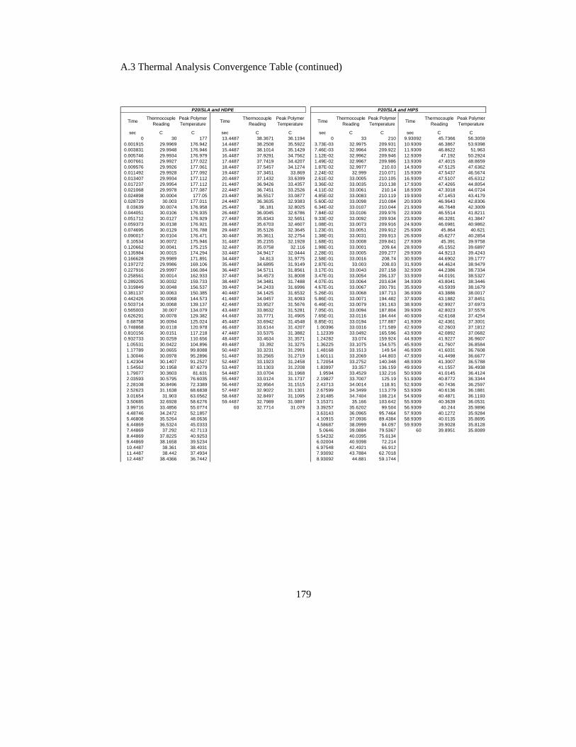
179

A.3 Thermal Analysis Convergence Table (continued)

TimeThermocouple

ReadingPeak Polymer Temperature

TimeThermocouple

ReadingPeak Polymer Temperature

TimeThermocouple

ReadingPeak Polymer Temperature

TimeThermocouple

ReadingPeak Polymer Temperature

sec C C sec C C sec C C sec C C0 30 177 13.4487 38.3671 36.1194 0 33 210 9.93092 45.7366 56.3059

0.001915 29.9969 176.942 14.4487 38.2508 35.5922 3.73E-03 32.9975 209.931 10.9309 46.3867 53.93980.003831 29.9948 176.946 15.4487 38.1014 35.1429 7.46E-03 32.9964 209.922 11.9309 46.8622 51.9630.005746 29.9934 176.979 16.4487 37.9291 34.7562 1.12E-02 32.9962 209.946 12.9309 47.192 50.29240.007661 29.9927 177.022 17.4487 37.7419 34.4207 1.49E-02 32.9967 209.986 13.9309 47.4015 48.86590.009576 29.9926 177.061 18.4487 37.5457 34.1274 1.87E-02 32.9977 210.03 14.9309 47.5125 47.63620.011492 29.9928 177.092 19.4487 37.3451 33.869 2.24E-02 32.999 210.071 15.9309 47.5437 46.56740.013407 29.9934 177.112 20.4487 37.1432 33.6399 2.61E-02 33.0005 210.105 16.9309 47.5107 45.63120.017237 29.9954 177.112 21.4487 36.9426 33.4357 3.36E-02 33.0035 210.138 17.9309 47.4265 44.80540.021068 29.9978 177.087 22.4487 36.7451 33.2526 4.11E-02 33.0061 210.14 18.9309 47.3018 44.07240.024898 30.0004 177.05 23.4487 36.5517 33.0877 4.85E-02 33.0083 210.119 19.9309 47.1453 43.41790.028729 30.003 177.011 24.4487 36.3635 32.9383 5.60E-02 33.0098 210.084 20.9309 46.9643 42.8306

0.03639 30.0074 176.958 25.4487 36.181 32.8025 6.34E-02 33.0107 210.044 21.9309 46.7648 42.30090.044051 30.0106 176.935 26.4487 36.0045 32.6786 7.84E-02 33.0106 209.976 22.9309 46.5514 41.82110.051712 30.0127 176.929 27.4487 35.8343 32.5651 9.33E-02 33.0092 209.934 23.9309 46.3281 41.38470.059373 30.0138 176.921 28.4487 35.6703 32.4607 1.08E-01 33.0073 209.916 24.9309 46.0981 40.98620.074695 30.0129 176.788 29.4487 35.5126 32.3645 1.23E-01 33.0051 209.912 25.9309 45.864 40.6210.090017 30.0104 176.471 30.4487 35.3611 32.2754 1.38E-01 33.0031 209.913 26.9309 45.6277 40.2854

0.10534 30.0072 175.946 31.4487 35.2155 32.1928 1.68E-01 33.0008 209.841 27.9309 45.391 39.97580.120662 30.0041 175.215 32.4487 35.0758 32.116 1.98E-01 33.0001 209.64 28.9309 45.1552 39.68970.135984 30.0015 174.294 33.4487 34.9417 32.0444 2.28E-01 33.0005 209.277 29.9309 44.9213 39.42430.166628 29.9989 171.891 34.4487 34.813 31.9775 2.58E-01 33.0016 208.74 30.9309 44.6902 39.17770.197272 29.9986 169.106 35.4487 34.6895 31.9149 2.87E-01 33.003 208.03 31.9309 44.4624 38.94790.227916 29.9997 166.084 36.4487 34.5711 31.8561 3.17E-01 33.0043 207.158 32.9309 44.2386 38.73340.258561 30.0014 162.933 37.4487 34.4573 31.8008 3.47E-01 33.0054 206.137 33.9309 44.0191 38.53270.289205 30.0032 159.733 38.4487 34.3481 31.7488 4.07E-01 33.0064 203.634 34.9309 43.8041 38.34460.319849 30.0048 156.537 39.4487 34.2433 31.6996 4.67E-01 33.0067 200.791 35.9309 43.5939 38.16790.381137 30.0063 150.385 40.4487 34.1425 31.6532 5.26E-01 33.0068 197.713 36.9309 43.3886 38.00170.442426 30.0068 144.573 41.4487 34.0457 31.6093 5.86E-01 33.0071 194.482 37.9309 43.1882 37.84510.503714 30.0068 139.137 42.4487 33.9527 31.5676 6.46E-01 33.0079 191.163 38.9309 42.9927 37.69730.565003 30.007 134.079 43.4487 33.8632 31.5281 7.05E-01 33.0094 187.804 39.9309 42.8023 37.55760.626291 30.0078 129.382 44.4487 33.7771 31.4905 7.65E-01 33.0116 184.444 40.9309 42.6168 37.4254

0.68758 30.0094 125.024 45.4487 33.6942 31.4548 8.85E-01 33.0194 177.887 41.9309 42.4361 37.30010.748868 30.0118 120.978 46.4487 33.6144 31.4207 1.00396 33.0316 171.589 42.9309 42.2603 37.18120.810156 30.0151 117.218 47.4487 33.5375 31.3882 1.12339 33.0492 165.596 43.9309 42.0892 37.06820.932733 30.0259 110.656 48.4487 33.4634 31.3571 1.24282 33.074 159.924 44.9309 41.9227 36.9607

1.05531 30.0422 104.896 49.4487 33.392 31.3275 1.36225 33.1075 154.575 45.9309 41.7607 36.85841.17789 30.0655 99.8088 50.4487 33.3231 31.2991 1.48168 33.1513 149.54 46.9309 41.6031 36.76081.30046 30.0978 95.2896 51.4487 33.2565 31.2719 1.60111 33.2069 144.803 47.9309 41.4498 36.66771.42304 30.1407 91.2527 52.4487 33.1923 31.2458 1.72054 33.2752 140.348 48.9309 41.3007 36.57881.54562 30.1958 87.6279 53.4487 33.1303 31.2208 1.83997 33.357 136.159 49.9309 41.1557 36.49381.79077 30.3603 81.631 54.4487 33.0704 31.1968 1.9594 33.4529 132.216 50.9309 41.0145 36.41242.03593 30.5795 76.6035 55.4487 33.0124 31.1737 2.19827 33.7007 125.19 51.9309 40.8772 36.33442.28108 30.8496 72.3389 56.4487 32.9564 31.1515 2.43713 34.0014 118.91 52.9309 40.7436 36.25972.52623 31.1638 68.6838 57.4487 32.9022 31.1301 2.67599 34.3499 113.279 53.9309 40.6136 36.18813.01654 31.903 63.0562 58.4487 32.8497 31.1095 2.91485 34.7404 108.214 54.9309 40.4871 36.11933.50685 32.6928 58.6276 59.4487 32.7989 31.0897 3.15371 35.166 103.642 55.9309 40.3639 36.05313.99716 33.4856 55.0774 60 32.7714 31.079 3.39257 35.6202 99.504 56.9309 40.244 35.98964.48746 34.2472 52.1857 3.63143 36.0965 95.7464 57.9309 40.1272 35.92845.46808 35.5264 48.0636 4.10915 37.0936 89.4384 58.9309 40.0135 35.86956.44869 36.5324 45.0333 4.58687 38.0999 84.097 59.9309 39.9028 35.81287.44869 37.292 42.7113 5.0646 39.0884 79.5367 60 39.8951 35.80898.44869 37.8225 40.9253 5.54232 40.0395 75.61349.44869 38.1658 39.5234 6.02004 40.9398 72.21410.4487 38.361 38.4031 6.97548 42.4921 66.91211.4487 38.442 37.4934 7.93092 43.7884 62.701812.4487 38.4366 36.7442 8.93092 44.881 59.1744

P20/SLA and HDPE P20/SLA and HIPS

180

A.3 Thermal Analysis Convergence Table (continued)

Time Thermocouple Reading

Peak Polymer Temperature

Time Thermocouple Reading

Peak Polymer Temperature

Time Thermocouple Reading

Peak Polymer

Temperature

sec C C sec C C sec C C0 30 177 44.3874 47.3999 51.8966 124.387 42.873 43.3108

0.001915 29.9969 176.939 45.3874 47.3293 51.663 125.387 42.8349 43.25960.003831 29.9948 176.944 46.3874 47.2581 51.4368 126.387 42.7971 43.2090.005746 29.9934 176.978 47.3874 47.1864 51.2176 127.387 42.7596 43.1590.007661 29.9927 177.022 48.3874 47.1143 51.0051 128.387 42.7225 43.10960.009576 29.9926 177.064 49.3874 47.042 50.7989 129.387 42.6857 43.06080.011492 29.9928 177.096 50.3874 46.9695 50.5987 130.387 42.6492 43.01250.013407 29.9934 177.117 51.3874 46.897 50.4043 131.387 42.613 42.96480.017237 29.9954 177.118 52.3874 46.8245 50.2154 132.387 42.5772 42.91760.021068 29.9978 177.092 53.3874 46.7521 50.0317 133.387 42.5416 42.8710.024898 30.0004 177.054 54.3874 46.6799 49.853 134.387 42.5064 42.82490.028729 30.003 177.014 55.3874 46.6079 49.6791 135.387 42.4715 42.7793

0.03639 30.0074 176.961 56.3874 46.5362 49.5097 136.387 42.4368 42.73420.044051 30.0106 176.94 57.3874 46.4649 49.3447 137.387 42.4025 42.68960.059373 30.013 176.91 58.3874 46.3939 49.1839 138.387 42.3684 42.64550.074695 30.0125 176.784 59.3874 46.3233 49.0271 139.387 42.3347 42.60180.090017 30.0102 176.499 60.3874 46.2532 48.8741 140.387 42.3012 42.55870.105339 30.0073 176.03 61.3874 46.1835 48.7248 141.387 42.268 42.5160.135983 30.0023 174.47 62.3874 46.1143 48.5791 142.387 42.2351 42.47370.166628 29.9996 172.471 63.3874 46.0456 48.4368 143.387 42.2024 42.43190.197272 29.9991 170.206 64.3874 45.9775 48.2978 144.387 42.17 42.3905

0.25856 30.0014 165.42 65.3874 45.9099 48.1619 145.387 42.1379 42.34960.319848 30.004 160.784 66.3874 45.8428 48.029 146.387 42.106 42.30910.381137 30.0057 156.469 67.3874 45.7763 47.8991 147.387 42.0745 42.2690.442425 30.0065 152.525 68.3874 45.7104 47.772 148.387 42.0431 42.22930.503713 30.0069 148.947 69.3874 45.645 47.6476 149.387 42.012 42.19

0.62629 30.0091 142.997 70.3874 45.5803 47.5259 150.387 41.9812 42.15110.748866 30.0144 137.993 71.3874 45.5161 47.4067 151.387 41.9506 42.11260.871443 30.0238 133.722 72.3874 45.4525 47.2899 152.387 41.9203 42.07450.994019 30.0384 130.023 73.3874 45.3895 47.1755 153.387 41.8902 42.0368

1.23917 30.0998 124.133 74.3874 45.3271 47.0634 154.387 41.8603 41.99941.48433 30.2049 119.284 75.3874 45.2653 46.9535 155.387 41.8307 41.96241.72948 30.3615 115.184 76.3874 45.204 46.8457 156.387 41.8013 41.92581.97463 30.5729 111.644 77.3874 45.1434 46.7401 157.387 41.7721 41.88952.46494 31.1932 106.025 78.3874 45.0834 46.6364 158.387 41.7432 41.85352.95524 31.9665 101.419 79.3874 45.0239 46.5347 159.387 41.7144 41.81793.44555 32.8439 97.5524 80.3874 44.965 46.4348 160.387 41.6859 41.78264.42616 34.7255 91.6781 81.3874 44.9067 46.3368 161.387 41.6577 41.74775.40678 36.5589 87.0491 82.3874 44.849 46.2406 162.387 41.6296 41.71316.38739 38.253 83.2962 83.3874 44.7919 46.1461 163.387 41.6018 41.67887.38739 39.7962 80.1313 84.3874 44.7353 46.0532 164.387 41.5741 41.64488.38739 41.147 77.4634 85.3874 44.6793 45.962 165.387 41.5467 41.61129.38739 42.3143 75.178 86.3874 44.6238 45.8724 166.387 41.5195 41.577810.3874 43.3146 73.1934 87.3874 44.5689 45.7843 167.387 41.4925 41.544811.3874 44.1668 71.45 88.3874 44.5145 45.6976 168.387 41.4656 41.51212.3874 44.8896 69.9031 89.3874 44.4607 45.6125 169.387 41.439 41.479613.3874 45.5007 68.5185 90.3874 44.4074 45.5287 170.387 41.4126 41.447414.3874 46.0156 67.2699 91.3874 44.3547 45.4463 171.387 41.3864 41.415515.3874 46.448 66.1363 92.3874 44.3024 45.3652 172.387 41.3604 41.383916.3874 46.8098 65.101 93.3874 44.2507 45.2855 173.387 41.3345 41.352617.3874 47.1112 64.1507 94.3874 44.1995 45.207 174.387 41.3089 41.321618.3874 47.3607 63.2742 95.3874 44.1488 45.1297 175.387 41.2834 41.290819.3874 47.5658 62.4624 96.3874 44.0986 45.0536 176.387 41.2581 41.260320.3874 47.7326 61.7077 97.3874 44.0489 44.9787 177.387 41.233 41.230121.3874 47.8666 61.0037 98.3874 43.9997 44.905 178.387 41.2081 41.200122.3874 47.9722 60.3449 99.3874 43.951 44.8323 179.387 41.1834 41.170323.3874 48.0534 59.7267 100.387 43.9027 44.7607 180.387 41.1588 41.140924.3874 48.1134 59.1451 101.387 43.855 44.6902 181.387 41.1344 41.111625.3874 48.1551 58.5965 102.387 43.8076 44.6208 182.387 41.1102 41.082626.3874 48.1809 58.0781 103.387 43.7608 44.5523 183.387 41.0862 41.053927.3874 48.193 57.587 104.387 43.7144 44.4848 184.387 41.0623 41.025428.3874 48.1931 57.1211 105.387 43.6684 44.4183 185.387 41.0386 40.997129.3874 48.1828 56.6781 106.387 43.6229 44.3527 186.387 41.0151 40.969130.3874 48.1634 56.2563 107.387 43.5778 44.288 187.387 40.9917 40.941231.3874 48.1363 55.8541 108.387 43.5332 44.2242 188.387 40.9685 40.913632.3874 48.1022 55.47 109.387 43.489 44.1613 189.387 40.9454 40.886333.3874 48.0623 55.1026 110.387 43.4452 44.0993 190.387 40.9225 40.8591

SLA and HDPE

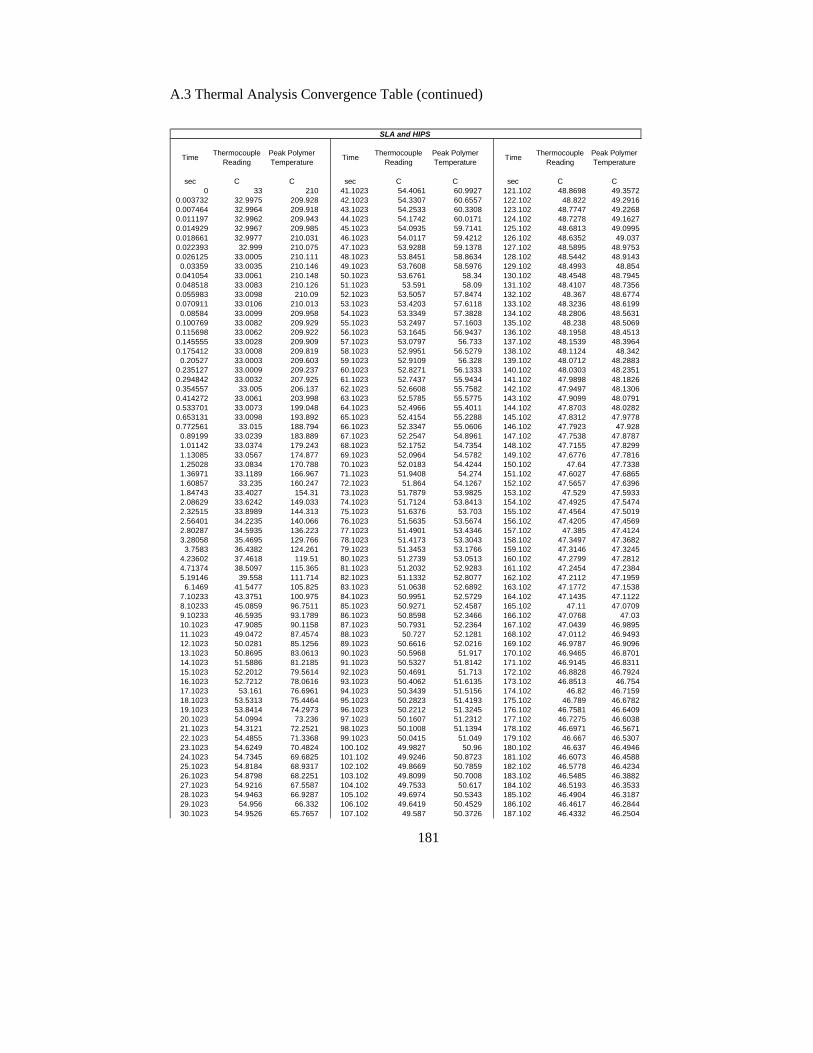
181

A.3 Thermal Analysis Convergence Table (continued)

TimeThermocouple

ReadingPeak Polymer Temperature

TimeThermocouple

ReadingPeak Polymer Temperature

TimeThermocouple

ReadingPeak Polymer Temperature

sec C C sec C C sec C C0 33 210 41.1023 54.4061 60.9927 121.102 48.8698 49.3572

0.003732 32.9975 209.928 42.1023 54.3307 60.6557 122.102 48.822 49.29160.007464 32.9964 209.918 43.1023 54.2533 60.3308 123.102 48.7747 49.22680.011197 32.9962 209.943 44.1023 54.1742 60.0171 124.102 48.7278 49.16270.014929 32.9967 209.985 45.1023 54.0935 59.7141 125.102 48.6813 49.09950.018661 32.9977 210.031 46.1023 54.0117 59.4212 126.102 48.6352 49.0370.022393 32.999 210.075 47.1023 53.9288 59.1378 127.102 48.5895 48.97530.026125 33.0005 210.111 48.1023 53.8451 58.8634 128.102 48.5442 48.9143

0.03359 33.0035 210.146 49.1023 53.7608 58.5976 129.102 48.4993 48.8540.041054 33.0061 210.148 50.1023 53.6761 58.34 130.102 48.4548 48.79450.048518 33.0083 210.126 51.1023 53.591 58.09 131.102 48.4107 48.73560.055983 33.0098 210.09 52.1023 53.5057 57.8474 132.102 48.367 48.67740.070911 33.0106 210.013 53.1023 53.4203 57.6118 133.102 48.3236 48.6199

0.08584 33.0099 209.958 54.1023 53.3349 57.3828 134.102 48.2806 48.56310.100769 33.0082 209.929 55.1023 53.2497 57.1603 135.102 48.238 48.50690.115698 33.0062 209.922 56.1023 53.1645 56.9437 136.102 48.1958 48.45130.145555 33.0028 209.909 57.1023 53.0797 56.733 137.102 48.1539 48.39640.175412 33.0008 209.819 58.1023 52.9951 56.5279 138.102 48.1124 48.342

0.20527 33.0003 209.603 59.1023 52.9109 56.328 139.102 48.0712 48.28830.235127 33.0009 209.237 60.1023 52.8271 56.1333 140.102 48.0303 48.23510.294842 33.0032 207.925 61.1023 52.7437 55.9434 141.102 47.9898 48.18260.354557 33.005 206.137 62.1023 52.6608 55.7582 142.102 47.9497 48.13060.414272 33.0061 203.998 63.1023 52.5785 55.5775 143.102 47.9099 48.07910.533701 33.0073 199.048 64.1023 52.4966 55.4011 144.102 47.8703 48.02820.653131 33.0098 193.892 65.1023 52.4154 55.2288 145.102 47.8312 47.97780.772561 33.015 188.794 66.1023 52.3347 55.0606 146.102 47.7923 47.928

0.89199 33.0239 183.889 67.1023 52.2547 54.8961 147.102 47.7538 47.87871.01142 33.0374 179.243 68.1023 52.1752 54.7354 148.102 47.7155 47.82991.13085 33.0567 174.877 69.1023 52.0964 54.5782 149.102 47.6776 47.78161.25028 33.0834 170.788 70.1023 52.0183 54.4244 150.102 47.64 47.73381.36971 33.1189 166.967 71.1023 51.9408 54.274 151.102 47.6027 47.68651.60857 33.235 160.247 72.1023 51.864 54.1267 152.102 47.5657 47.63961.84743 33.4027 154.31 73.1023 51.7879 53.9825 153.102 47.529 47.59332.08629 33.6242 149.033 74.1023 51.7124 53.8413 154.102 47.4925 47.54742.32515 33.8989 144.313 75.1023 51.6376 53.703 155.102 47.4564 47.50192.56401 34.2235 140.066 76.1023 51.5635 53.5674 156.102 47.4205 47.45692.80287 34.5935 136.223 77.1023 51.4901 53.4346 157.102 47.385 47.41243.28058 35.4695 129.766 78.1023 51.4173 53.3043 158.102 47.3497 47.3682

3.7583 36.4382 124.261 79.1023 51.3453 53.1766 159.102 47.3146 47.32454.23602 37.4618 119.51 80.1023 51.2739 53.0513 160.102 47.2799 47.28124.71374 38.5097 115.365 81.1023 51.2032 52.9283 161.102 47.2454 47.23845.19146 39.558 111.714 82.1023 51.1332 52.8077 162.102 47.2112 47.1959

6.1469 41.5477 105.825 83.1023 51.0638 52.6892 163.102 47.1772 47.15387.10233 43.3751 100.975 84.1023 50.9951 52.5729 164.102 47.1435 47.11228.10233 45.0859 96.7511 85.1023 50.9271 52.4587 165.102 47.11 47.07099.10233 46.5935 93.1789 86.1023 50.8598 52.3466 166.102 47.0768 47.0310.1023 47.9085 90.1158 87.1023 50.7931 52.2364 167.102 47.0439 46.989511.1023 49.0472 87.4574 88.1023 50.727 52.1281 168.102 47.0112 46.949312.1023 50.0281 85.1256 89.1023 50.6616 52.0216 169.102 46.9787 46.909613.1023 50.8695 83.0613 90.1023 50.5968 51.917 170.102 46.9465 46.870114.1023 51.5886 81.2185 91.1023 50.5327 51.8142 171.102 46.9145 46.831115.1023 52.2012 79.5614 92.1023 50.4691 51.713 172.102 46.8828 46.792416.1023 52.7212 78.0616 93.1023 50.4062 51.6135 173.102 46.8513 46.75417.1023 53.161 76.6961 94.1023 50.3439 51.5156 174.102 46.82 46.715918.1023 53.5313 75.4464 95.1023 50.2823 51.4193 175.102 46.789 46.678219.1023 53.8414 74.2973 96.1023 50.2212 51.3245 176.102 46.7581 46.640920.1023 54.0994 73.236 97.1023 50.1607 51.2312 177.102 46.7275 46.603821.1023 54.3121 72.2521 98.1023 50.1008 51.1394 178.102 46.6971 46.567122.1023 54.4855 71.3368 99.1023 50.0415 51.049 179.102 46.667 46.530723.1023 54.6249 70.4824 100.102 49.9827 50.96 180.102 46.637 46.494624.1023 54.7345 69.6825 101.102 49.9246 50.8723 181.102 46.6073 46.458825.1023 54.8184 68.9317 102.102 49.8669 50.7859 182.102 46.5778 46.423426.1023 54.8798 68.2251 103.102 49.8099 50.7008 183.102 46.5485 46.388227.1023 54.9216 67.5587 104.102 49.7533 50.617 184.102 46.5193 46.353328.1023 54.9463 66.9287 105.102 49.6974 50.5343 185.102 46.4904 46.318729.1023 54.956 66.332 106.102 49.6419 50.4529 186.102 46.4617 46.284430.1023 54.9526 65.7657 107.102 49.587 50.3726 187.102 46.4332 46.2504

SLA and HIPS

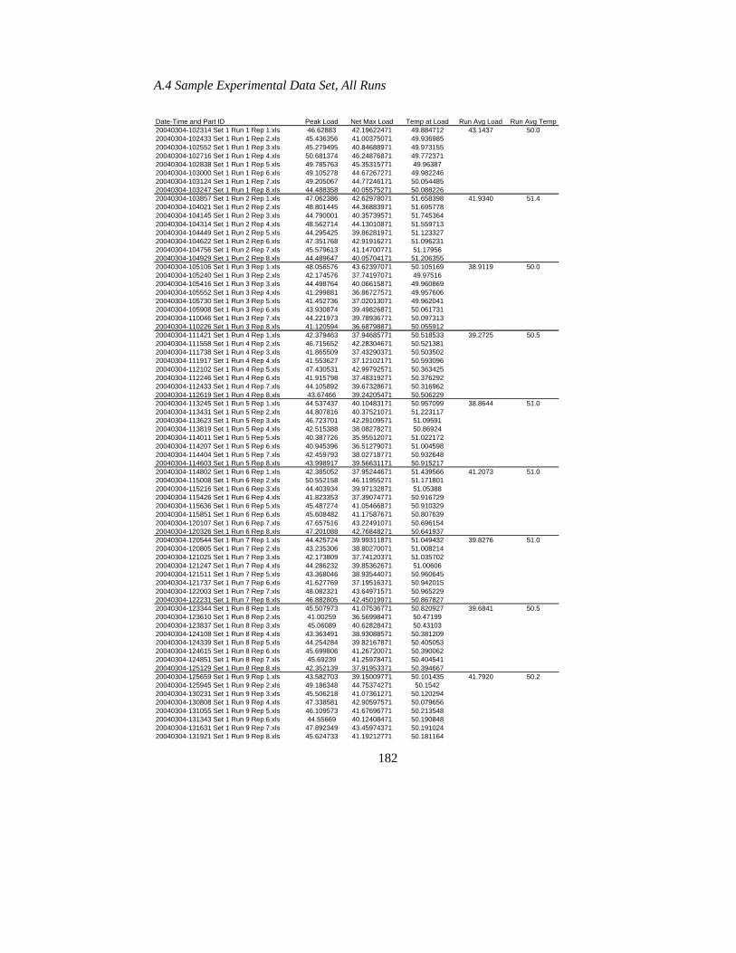
182

A.4 Sample Experimental Data Set, All Runs

Date-Time and Part ID Peak Load Net Max Load Temp at Load Run Avg Load Run Avg Temp20040304-102314 Set 1 Run 1 Rep 1.xls 46.62883 42.19622471 49.884712 43.1437 50.020040304-102433 Set 1 Run 1 Rep 2.xls 45.436356 41.00375071 49.93698520040304-102552 Set 1 Run 1 Rep 3.xls 45.279495 40.84688971 49.97315520040304-102716 Set 1 Run 1 Rep 4.xls 50.681374 46.24876871 49.77237120040304-102838 Set 1 Run 1 Rep 5.xls 49.785763 45.35315771 49.9638720040304-103000 Set 1 Run 1 Rep 6.xls 49.105278 44.67267271 49.98224620040304-103124 Set 1 Run 1 Rep 7.xls 49.205067 44.77246171 50.05448520040304-103247 Set 1 Run 1 Rep 8.xls 44.488358 40.05575271 50.08822620040304-103857 Set 1 Run 2 Rep 1.xls 47.062386 42.62978071 51.658398 41.9340 51.420040304-104021 Set 1 Run 2 Rep 2.xls 48.801445 44.36883971 51.69577820040304-104145 Set 1 Run 2 Rep 3.xls 44.790001 40.35739571 51.74536420040304-104314 Set 1 Run 2 Rep 4.xls 48.562714 44.13010871 51.55971320040304-104449 Set 1 Run 2 Rep 5.xls 44.295425 39.86281971 51.12332720040304-104622 Set 1 Run 2 Rep 6.xls 47.351768 42.91916271 51.09623120040304-104756 Set 1 Run 2 Rep 7.xls 45.579613 41.14700771 51.1795620040304-104929 Set 1 Run 2 Rep 8.xls 44.489647 40.05704171 51.20635520040304-105106 Set 1 Run 3 Rep 1.xls 48.056576 43.62397071 50.105169 38.9119 50.020040304-105240 Set 1 Run 3 Rep 2.xls 42.174576 37.74197071 49.9751620040304-105416 Set 1 Run 3 Rep 3.xls 44.498764 40.06615871 49.96086920040304-105552 Set 1 Run 3 Rep 4.xls 41.299881 36.86727571 49.95760620040304-105730 Set 1 Run 3 Rep 5.xls 41.452736 37.02013071 49.96204120040304-105908 Set 1 Run 3 Rep 6.xls 43.930874 39.49826871 50.06173120040304-110046 Set 1 Run 3 Rep 7.xls 44.221973 39.78936771 50.09731320040304-110226 Set 1 Run 3 Rep 8.xls 41.120594 36.68798871 50.05591220040304-111421 Set 1 Run 4 Rep 1.xls 42.379463 37.94685771 50.518533 39.2725 50.520040304-111558 Set 1 Run 4 Rep 2.xls 46.715652 42.28304671 50.52138120040304-111738 Set 1 Run 4 Rep 3.xls 41.865509 37.43290371 50.50350220040304-111917 Set 1 Run 4 Rep 4.xls 41.553627 37.12102171 50.59309620040304-112102 Set 1 Run 4 Rep 5.xls 47.430531 42.99792571 50.36342520040304-112246 Set 1 Run 4 Rep 6.xls 41.915798 37.48319271 50.37629220040304-112433 Set 1 Run 4 Rep 7.xls 44.105892 39.67328671 50.31696220040304-112619 Set 1 Run 4 Rep 8.xls 43.67466 39.24205471 50.50622920040304-113245 Set 1 Run 5 Rep 1.xls 44.537437 40.10483171 50.957099 38.8644 51.020040304-113431 Set 1 Run 5 Rep 2.xls 44.807816 40.37521071 51.22311720040304-113623 Set 1 Run 5 Rep 3.xls 46.723701 42.29109571 51.0959120040304-113819 Set 1 Run 5 Rep 4.xls 42.515388 38.08278271 50.8692420040304-114011 Set 1 Run 5 Rep 5.xls 40.387726 35.95512071 51.02217220040304-114207 Set 1 Run 5 Rep 6.xls 40.945396 36.51279071 51.00459820040304-114404 Set 1 Run 5 Rep 7.xls 42.459793 38.02718771 50.93264820040304-114603 Set 1 Run 5 Rep 8.xls 43.998917 39.56631171 50.91521720040304-114802 Set 1 Run 6 Rep 1.xls 42.385052 37.95244671 51.439566 41.2073 51.020040304-115008 Set 1 Run 6 Rep 2.xls 50.552158 46.11955271 51.17180120040304-115216 Set 1 Run 6 Rep 3.xls 44.403934 39.97132871 51.0538820040304-115426 Set 1 Run 6 Rep 4.xls 41.823353 37.39074771 50.91672920040304-115636 Set 1 Run 6 Rep 5.xls 45.487274 41.05466871 50.91032920040304-115851 Set 1 Run 6 Rep 6.xls 45.608482 41.17587671 50.80763920040304-120107 Set 1 Run 6 Rep 7.xls 47.657516 43.22491071 50.69615420040304-120326 Set 1 Run 6 Rep 8.xls 47.201088 42.76848271 50.64193720040304-120544 Set 1 Run 7 Rep 1.xls 44.425724 39.99311871 51.049432 39.8276 51.020040304-120805 Set 1 Run 7 Rep 2.xls 43.235306 38.80270071 51.00821420040304-121025 Set 1 Run 7 Rep 3.xls 42.173809 37.74120371 51.03570220040304-121247 Set 1 Run 7 Rep 4.xls 44.286232 39.85362671 51.0060620040304-121511 Set 1 Run 7 Rep 5.xls 43.368046 38.93544071 50.96064520040304-121737 Set 1 Run 7 Rep 6.xls 41.627769 37.19516371 50.94201520040304-122003 Set 1 Run 7 Rep 7.xls 48.082321 43.64971571 50.96522920040304-122231 Set 1 Run 7 Rep 8.xls 46.882805 42.45019971 50.86782720040304-123344 Set 1 Run 8 Rep 1.xls 45.507973 41.07536771 50.820927 39.6841 50.520040304-123610 Set 1 Run 8 Rep 2.xls 41.00259 36.56998471 50.4719920040304-123837 Set 1 Run 8 Rep 3.xls 45.06089 40.62828471 50.4310320040304-124108 Set 1 Run 8 Rep 4.xls 43.363491 38.93088571 50.38120920040304-124339 Set 1 Run 8 Rep 5.xls 44.254284 39.82167871 50.40505320040304-124615 Set 1 Run 8 Rep 6.xls 45.699806 41.26720071 50.39006220040304-124851 Set 1 Run 8 Rep 7.xls 45.69239 41.25978471 50.40454120040304-125129 Set 1 Run 8 Rep 8.xls 42.352139 37.91953371 50.39466720040304-125659 Set 1 Run 9 Rep 1.xls 43.582703 39.15009771 50.101435 41.7920 50.220040304-125945 Set 1 Run 9 Rep 2.xls 49.186348 44.75374271 50.154220040304-130231 Set 1 Run 9 Rep 3.xls 45.506218 41.07361271 50.12029420040304-130808 Set 1 Run 9 Rep 4.xls 47.338581 42.90597571 50.07965620040304-131055 Set 1 Run 9 Rep 5.xls 46.109573 41.67696771 50.21354820040304-131343 Set 1 Run 9 Rep 6.xls 44.55669 40.12408471 50.19084820040304-131631 Set 1 Run 9 Rep 7.xls 47.892349 43.45974371 50.19102420040304-131921 Set 1 Run 9 Rep 8.xls 45.624733 41.19212771 50.181164

183

A.4 Sample Experimental Data Set, All Runs (continued)

Date-Time and Part ID Peak Load Net Max Load Temp at Load Run Avg Load Run Avg Temp20040305-091132 Set 1 Run 10 Rep 1.xls 47.874283 43.44167771 49.551394 41.7107 49.620040305-091217 Set 1 Run 10 Rep 2.xls 46.989723 42.55711771 49.37364720040305-091301 Set 1 Run 10 Rep 3.xls 46.881813 42.44920771 49.66121820040305-091349 Set 1 Run 10 Rep 4.xls 45.736076 41.30347071 49.48452920040305-091433 Set 1 Run 10 Rep 5.xls 45.029144 40.59653871 49.62528120040305-091521 Set 1 Run 10 Rep 6.xls 46.069248 41.63664271 49.70783720040305-091609 Set 1 Run 10 Rep 7.xls 48.469646 44.03704071 49.69173620040305-091658 Set 1 Run 10 Rep 8.xls 42.096375 37.66376971 49.54598920040305-092152 Set 1 Run 11 Rep 1.xls 44.725861 40.29325571 50.649783 41.5225 49.420040305-092303 Set 1 Run 11 Rep 2.xls 44.587673 40.15506771 50.05003120040305-092421 Set 1 Run 11 Rep 3.xls 42.717182 38.28457671 49.42305820040305-092535 Set 1 Run 11 Rep 4.xls 46.337166 41.90456071 49.43257820040305-092653 Set 1 Run 11 Rep 5.xls 44.815929 40.38332371 49.19435220040305-092816 Set 1 Run 11 Rep 6.xls 45.658592 41.22598671 48.90143820040305-092938 Set 1 Run 11 Rep 7.xls 49.946003 45.51339771 48.90898620040305-093058 Set 1 Run 11 Rep 8.xls 48.852619 44.42001371 49.01373920040305-093332 Set 1 Run 12 Rep 1.xls 51.720848 47.28824271 49.580786 43.5216 49.520040305-093449 Set 1 Run 12 Rep 2.xls 45.144958 40.71235271 49.47220220040305-093609 Set 1 Run 12 Rep 3.xls 43.349007 38.91640171 49.34560120040305-093730 Set 1 Run 12 Rep 4.xls 51.384926 46.95232071 49.33205520040305-093852 Set 1 Run 12 Rep 5.xls 50.378567 45.94596171 49.24517820040305-094011 Set 1 Run 12 Rep 6.xls 41.728935 37.29632971 49.55756420040305-094129 Set 1 Run 12 Rep 7.xls 48.978333 44.54572771 49.72049820040305-094249 Set 1 Run 12 Rep 8.xls 50.947769 46.51516371 49.87151320040305-094533 Set 1 Run 13 Rep 1.xls 41.8722 37.43959471 48.736814 40.4794 49.120040305-094652 Set 1 Run 13 Rep 2.xls 43.347034 38.91442871 48.67456420040305-094807 Set 1 Run 13 Rep 3.xls 44.334808 39.90220271 48.83470220040305-094919 Set 1 Run 13 Rep 4.xls 45.608547 41.17594171 49.22759220040305-095033 Set 1 Run 13 Rep 5.xls 49.756042 45.32343671 49.3911620040305-095150 Set 1 Run 13 Rep 6.xls 45.773117 41.34051171 49.2881620040305-095307 Set 1 Run 13 Rep 7.xls 40.27779 35.84518471 49.36791420040305-095422 Set 1 Run 13 Rep 8.xls 48.326248 43.89364271 49.55803220040305-100925 Set 1 Run 14 Rep 1.xls 43.114841 38.68223571 50.717812 38.5078 50.620040305-101047 Set 1 Run 14 Rep 2.xls 41.929817 37.49721171 50.76961520040305-101219 Set 1 Run 14 Rep 3.xls 40.761803 36.32919771 50.15043520040305-101340 Set 1 Run 14 Rep 4.xls 44.940529 40.50792371 50.77556720040305-101504 Set 1 Run 14 Rep 5.xls 44.202026 39.76942071 50.93581120040305-101632 Set 1 Run 14 Rep 6.xls 45.258545 40.82593971 50.82292720040305-101806 Set 1 Run 14 Rep 7.xls 39.655685 35.22307971 50.44938320040305-101943 Set 1 Run 14 Rep 8.xls 43.660015 39.22740971 50.22961620040305-102447 Set 1 Run 15 Rep 1.xls 43.201645 38.76903971 50.501971 39.2605 50.720040305-102617 Set 1 Run 15 Rep 2.xls 44.945435 40.51282971 50.60903820040305-102747 Set 1 Run 15 Rep 3.xls 44.624767 40.19216171 50.68684520040305-102919 Set 1 Run 15 Rep 4.xls 41.508282 37.07567671 50.74748220040305-103050 Set 1 Run 15 Rep 5.xls 43.016941 38.58433571 50.83082520040305-103224 Set 1 Run 15 Rep 6.xls 40.242275 35.80966971 50.82224420040305-103358 Set 1 Run 15 Rep 7.xls 48.910042 44.47743671 50.77231120040305-103532 Set 1 Run 15 Rep 8.xls 43.095409 38.66280371 50.92340220040305-103715 Set 1 Run 16 Rep 1.xls 45.12886 40.69625471 50.471526 38.2203 50.520040305-103855 Set 1 Run 16 Rep 2.xls 45.127762 40.69515671 50.41387820040305-104036 Set 1 Run 16 Rep 3.xls 42.580982 38.14837671 50.51411720040305-104221 Set 1 Run 16 Rep 4.xls 41.723831 37.29122571 50.40225320040305-104407 Set 1 Run 16 Rep 5.xls 44.49881 40.06620471 50.35189920040305-104556 Set 1 Run 16 Rep 6.xls 37.737038 33.30443271 50.2258920040305-104735 Set 1 Run 16 Rep 7.xls 37.382568 32.94996271 50.76344420040305-104916 Set 1 Run 16 Rep 8.xls 47.043259 42.61065371 50.89240820040305-105845 Set 1 Run 17 Rep 1.xls 41.832466 37.39986071 51.569878 39.0911 50.720040305-110035 Set 1 Run 17 Rep 2.xls 40.071449 35.63884371 51.32120820040305-110236 Set 1 Run 17 Rep 3.xls 43.794182 39.36157671 50.66980120040305-110443 Set 1 Run 17 Rep 4.xls 41.143127 36.71052171 50.37951420040305-110647 Set 1 Run 17 Rep 5.xls 39.029778 34.59717271 50.39036220040305-110854 Set 1 Run 17 Rep 6.xls 46.641609 42.20900371 50.40425120040305-111102 Set 1 Run 17 Rep 7.xls 47.707619 43.27501371 50.40962520040305-111310 Set 1 Run 17 Rep 8.xls 47.969162 43.53655671 50.40358420040305-112848 Set 1 Run 18 Rep 1.xls 39.171555 34.73894971 49.835092 39.3858 50.120040305-113056 Set 1 Run 18 Rep 2.xls 48.006432 43.57382671 50.09345920040305-113310 Set 1 Run 18 Rep 3.xls 47.755684 43.32307871 49.99326120040305-113522 Set 1 Run 18 Rep 4.xls 39.958481 35.52587571 50.17830120040305-113735 Set 1 Run 18 Rep 5.xls 40.581181 36.14857571 50.23739420040305-113954 Set 1 Run 18 Rep 6.xls 47.601276 43.16867071 50.09685420040305-114208 Set 1 Run 18 Rep 7.xls 44.750404 40.31779871 50.24234920040305-114427 Set 1 Run 18 Rep 8.xls 42.72242 38.28981471 50.195285

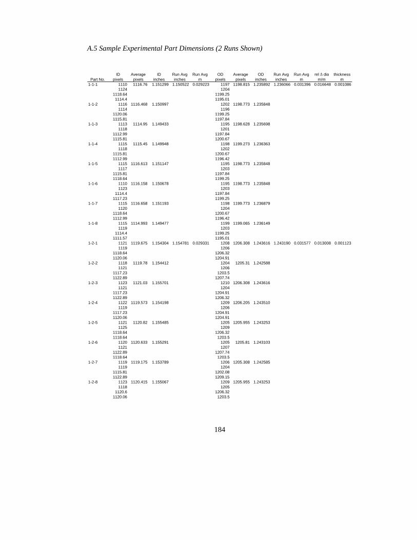
184

A.5 Sample Experimental Part Dimensions (2 Runs Shown)

ID Average ID Run Avg Run Avg OD Average OD Run Avg Run Avg rel ∆ dia thicknessPart No. pixels pixels inches inches m pixels pixels inches inches m m/m m

1-1-1 1110 1116.76 1.151299 1.150522 0.029223 1197 1198.815 1.235892 1.236066 0.031396 0.016648 0.0010861124 1204

1118.64 1199.251114.4 1195.01

1-1-2 1116 1116.468 1.150997 1202 1198.773 1.2358481114 1196

1120.06 1199.251115.81 1197.84

1-1-3 1113 1114.95 1.149433 1195 1198.628 1.2356981118 1201

1112.99 1197.841115.81 1200.67

1-1-4 1115 1115.45 1.149948 1198 1199.273 1.2363631118 1202

1115.81 1200.671112.99 1196.42

1-1-5 1115 1116.613 1.151147 1195 1198.773 1.2358481117 1203

1115.81 1197.841118.64 1199.25

1-1-6 1110 1116.158 1.150678 1195 1198.773 1.2358481123 1203

1114.4 1197.841117.23 1199.25

1-1-7 1115 1116.658 1.151193 1198 1199.773 1.2368791120 1204

1118.64 1200.671112.99 1196.42

1-1-8 1115 1114.993 1.149477 1199 1199.065 1.2361491119 1203

1114.4 1199.251111.57 1195.01

1-2-1 1121 1119.675 1.154304 1.154781 0.029331 1208 1206.308 1.243616 1.243190 0.031577 0.013008 0.0011231119 1206

1118.64 1206.321120.06 1204.91

1-2-2 1118 1119.78 1.154412 1204 1205.31 1.2425881121 1206

1117.23 1203.51122.89 1207.74

1-2-3 1123 1121.03 1.155701 1210 1206.308 1.2436161121 1204

1117.23 1204.911122.89 1206.32

1-2-4 1122 1119.573 1.154198 1209 1206.205 1.2435101119 1206

1117.23 1204.911120.06 1204.91

1-2-5 1121 1120.82 1.155485 1205 1205.955 1.2432531125 1209

1118.64 1206.321118.64 1203.5

1-2-6 1120 1120.633 1.155291 1205 1205.81 1.2431031121 1207

1122.89 1207.741118.64 1203.5

1-2-7 1119 1119.175 1.153789 1206 1205.308 1.2425851119 1204

1115.81 1202.081122.89 1209.15

1-2-8 1123 1120.415 1.155067 1209 1205.955 1.2432531118 1205

1120.6 1206.321120.06 1203.5

185

A.6 Experimental Data and Calculated Coefficient of Friction (Menges), Run Average

Insert/ Thermoplastic Tpack Tcool Ppack

Ejection Force (N)

Ejection Temp (oC)

Modulus at Ejection

Temp (Pa)

Relative Change in Dia (m/m)

Thickness (m) CoF

P-20 -1 -1 -1 177.1534 51.0 69000000 0.013299 0.001075 0.589265HDPE -1 -1 0 183.2899 51.0 69000000 0.012021 0.001109 0.653811

-1 -1 1 186.5225 51.4 65400000 0.013008 0.001123 0.640622-1 0 -1 176.5148 50.5 71500000 0.013940 0.00108 0.537958-1 0 0 185.891 50.2 73000000 0.012097 0.001114 0.619705-1 0 1 172.8689 51.0 69000000 0.011691 0.001121 0.627208-1 1 -1 191.9032 50.0 74000000 0.016648 0.001086 0.470372-1 1 0 174.6842 50.5 71500000 0.011819 0.00111 0.610927-1 1 1 173.0801 50.0 74000000 0.012125 0.001127 0.5613181 -1 -1 184.6922 49.4 78800000 0.012311 0.00107 0.5836841 -1 0 193.5839 49.5 78000000 0.011043 0.001118 0.6594971 -1 1 173.8771 50.7 70500000 0.009859 0.001123 0.7306781 0 -1 171.2827 50.6 71000000 0.012184 0.001066 0.6091971 0 0 174.6307 50.7 70500000 0.010684 0.001114 0.6828871 0 1 175.1881 50.1 73500000 0.008880 0.001125 0.7827971 1 -1 170.0038 50.5 71500000 0.012579 0.001074 0.5771231 1 0 180.0522 49.1 81200000 0.011084 0.001115 0.5887281 1 1 185.5291 49.6 77200000 0.010279 0.001126 0.681465

P-20 -1 -1 -1 343.9689 51.0 580000000 0.003089 0.001138 0.553423HIPS -1 -1 0 376.3673 51.1 573000000 0.003377 0.00114 0.559850

-1 -1 1 401.4804 51.1 573000000 0.002935 0.001144 0.684961-1 0 -1 346.1149 50.8 592400000 0.003301 0.001134 0.511977-1 0 0 385.5599 50.8 592400000 0.003565 0.001146 0.522718-1 0 1 408.2617 51.0 580000000 0.002989 0.001133 0.681704-1 1 -1 384.5955 50.4 617200000 0.003788 0.001139 0.473993-1 1 0 381.943 50.2 629600000 0.002896 0.001131 0.607589-1 1 1 403.7004 50.2 629600000 0.00354 0.00115 0.5168811 -1 -1 376.9719 50.5 611000000 0.003199 0.001124 0.5630751 -1 0 395.2322 51.1 573000000 0.003444 0.001138 0.5773281 -1 1 393.3786 51.5 545000000 0.001107 0.00114 1.8767601 0 -1 369.1949 50.6 604800000 0.002796 0.001139 0.6289231 0 0 390.8133 50.8 592400000 0.002337 0.001137 0.8147461 0 1 391.7333 50.9 586200000 0.001826 0.001146 1.0474711 1 -1 351.6246 50.4 617200000 0.002424 0.001141 0.6757131 1 0 394.7653 49.6 673200000 0.002791 0.001137 0.6062391 1 1 424.4616 48.9 728000000 0.003016 0.001127 0.562590

ST-100 -1 -1 -1 182.3003 50.9 69500000 0.005901 0.00104 1.402205HDPE -1 -1 0 190.0239 50.9 69500000 0.006708 0.001108 1.207056

-1 -1 1 209.7913 50.3 72500000 0.007395 0.001116 1.150452-1 0 -1 177.4434 50.3 72500000 0.006204 0.001045 1.238469-1 0 0 196.6074 50.2 73000000 0.006976 0.001109 1.142516-1 0 1 194.3292 51.4 65400000 0.007264 0.001122 1.196203-1 1 -1 196.1544 49.1 81200000 0.012154 0.001093 0.596783-1 1 0 201.6826 50.2 73000000 0.007462 0.001105 1.099385-1 1 1 208.7471 49.6 77200000 0.006877 0.001113 1.1591081 -1 -1 173.9534 50.8 70000000 0.010785 0.00103 0.7338391 -1 0 185.8118 50 74000000 0.011344 0.001103 0.6581921 -1 1 184.4146 50.6 71000000 0.010469 0.001122 0.7253771 0 -1 172.1205 50.4 72000000 0.010469 0.001031 0.7264031 0 0 178.8341 50.2 73000000 0.010979 0.001109 0.6599691 0 1 180.8674 50.2 73000000 0.010258 0.001119 0.7078421 1 -1 170.97 50.2 73000000 0.011443 0.001055 0.6363091 1 0 186.8184 49.3 79600000 0.01105 0.001104 0.6311151 1 1 184.1281 48.6 85200000 0.010809 0.001114 0.589072

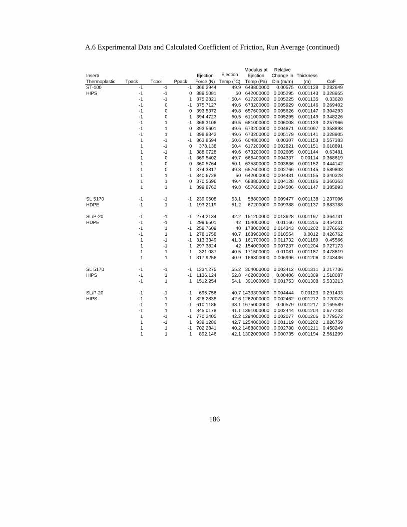
186

A.6 Experimental Data and Calculated Coefficient of Friction, Run Average (continued)

Insert/ Thermoplastic Tpack Tcool Ppack

Ejection Force (N)

Ejection Temp (oC)

Modulus at Ejection

Temp (Pa)

Relative Change in Dia (m/m)

Thickness (m) CoF

ST-100 -1 -1 -1 366.2944 49.9 649800000 0.00575 0.001138 0.282649HIPS -1 -1 0 389.5081 50 642000000 0.005295 0.001143 0.328955

-1 -1 1 375.2821 50.4 617200000 0.005225 0.001135 0.33628-1 0 -1 375.7127 49.6 673200000 0.005929 0.001146 0.269402-1 0 0 393.5372 49.8 657600000 0.005626 0.001147 0.304293-1 0 1 394.4723 50.5 611000000 0.005295 0.001149 0.348226-1 1 -1 366.3106 49.5 681000000 0.006008 0.001139 0.257966-1 1 0 393.5601 49.6 673200000 0.004871 0.001097 0.358898-1 1 1 398.8342 49.6 673200000 0.005179 0.001141 0.3289051 -1 -1 363.8594 50.6 604800000 0.00307 0.001153 0.5573831 -1 0 378.138 50.4 617200000 0.002821 0.001151 0.6188911 -1 1 388.0728 49.6 673200000 0.002605 0.001144 0.634811 0 -1 369.5402 49.7 665400000 0.004337 0.00114 0.3686191 0 0 360.5764 50.1 635800000 0.003636 0.001152 0.4441421 0 1 374.3817 49.8 657600000 0.002766 0.001145 0.5898031 1 -1 340.6728 50 642000000 0.004431 0.001155 0.3403281 1 0 370.5696 49.4 688800000 0.004128 0.001186 0.3603631 1 1 399.8762 49.8 657600000 0.004506 0.001147 0.385893

SL 5170 -1 -1 -1 239.0608 53.1 58800000 0.009477 0.001138 1.237096HDPE -1 1 -1 193.2119 51.2 67200000 0.009388 0.001137 0.883788

SL/P-20 -1 -1 -1 274.2134 42.2 151200000 0.013628 0.001197 0.364731HDPE -1 -1 1 299.6501 42 154000000 0.01166 0.001205 0.454231

-1 1 -1 258.7609 40 178000000 0.014343 0.001202 0.276662-1 1 1 278.1758 40.7 168900000 0.010554 0.0012 0.4267621 -1 -1 313.3349 41.3 161700000 0.011732 0.001189 0.455661 -1 1 297.3824 42 154000000 0.007237 0.001204 0.7271731 1 -1 321.087 40.5 171500000 0.01081 0.001187 0.4786191 1 1 317.9256 40.9 166300000 0.006996 0.001206 0.743436

SL 5170 -1 -1 -1 1334.275 55.2 304000000 0.003412 0.001311 3.217736HIPS -1 1 -1 1136.124 52.8 462000000 0.00406 0.001309 1.518087

-1 1 1 1512.254 54.1 391000000 0.001753 0.001308 5.533213

SL/P-20 -1 -1 -1 695.756 40.7 1433300000 0.004444 0.00123 0.291433HIPS -1 -1 1 826.2838 42.6 1262000000 0.002462 0.001212 0.720073

-1 1 -1 610.1186 38.1 1675000000 0.00579 0.001217 0.169589-1 1 1 845.0178 41.1 1391000000 0.002444 0.001204 0.6772331 -1 -1 770.2405 42.2 1294000000 0.002077 0.001206 0.7795721 -1 1 939.1286 42.7 1254000000 0.001119 0.001202 1.8267591 1 -1 702.2841 40.2 1488800000 0.002788 0.001211 0.4582491 1 1 892.146 42.1 1302000000 0.000735 0.001194 2.561299

187

A.7 Analysis of Variance Tables by Set

General Linear Model: P-20 and HDPE EF Set 1 versus Packing Time, Cooling Time, Packing Pressure Factor Type Levels Values Packing fixed 2 2 6 Cooling fixed 3 5 10 15 Packing fixed 3 0 5 10 Analysis of Variance for EF Set 1, using Adjusted SS for Tests Source DF Seq SS Adj SS Adj MS F P Packing 1 3.836 3.836 3.836 0.54 0.465 Cooling 2 149.135 149.135 74.568 10.44 0.000 Packing 2 13.938 13.938 6.969 0.98 0.380 Packing*Cooling 2 36.255 36.255 18.128 2.54 0.083 Packing*Packing 2 3.204 3.204 1.602 0.22 0.799 Cooling*Packing 4 40.352 40.352 10.088 1.41 0.234 Packing*Cooling*Packing 4 106.985 106.985 26.746 3.75 0.006 Error 126 899.771 899.771 7.141 Total 143 1253.478

General Linear Model: P-20 and HIPS EF Set 2 versus Packing Time, Cooling Time, Packing Pressure (One Outlier Removed) Factor Type Levels Values Packing fixed 2 2 6 Cooling fixed 3 5 10 15 Packing fixed 3 0 5 10 Analysis of Variance for EF Set 2, using Adjusted SS for Tests Source DF Seq SS Adj SS Adj MS F P Packing 1 89.91 95.44 95.44 8.84 0.004 Cooling 2 1059.86 1063.93 531.97 49.29 0.000 Packing 2 119.56 114.30 57.15 5.30 0.006 Packing*Cooling 2 166.61 158.03 79.01 7.32 0.001 Packing*Packing 2 245.27 254.54 127.27 11.79 0.000 Cooling*Packing 4 689.01 691.83 172.96 16.03 0.000 Packing*Cooling*Packing 4 863.76 863.76 215.94 20.01 0.000 Error 125 1349.12 1349.12 10.79 Total 142 4583.09

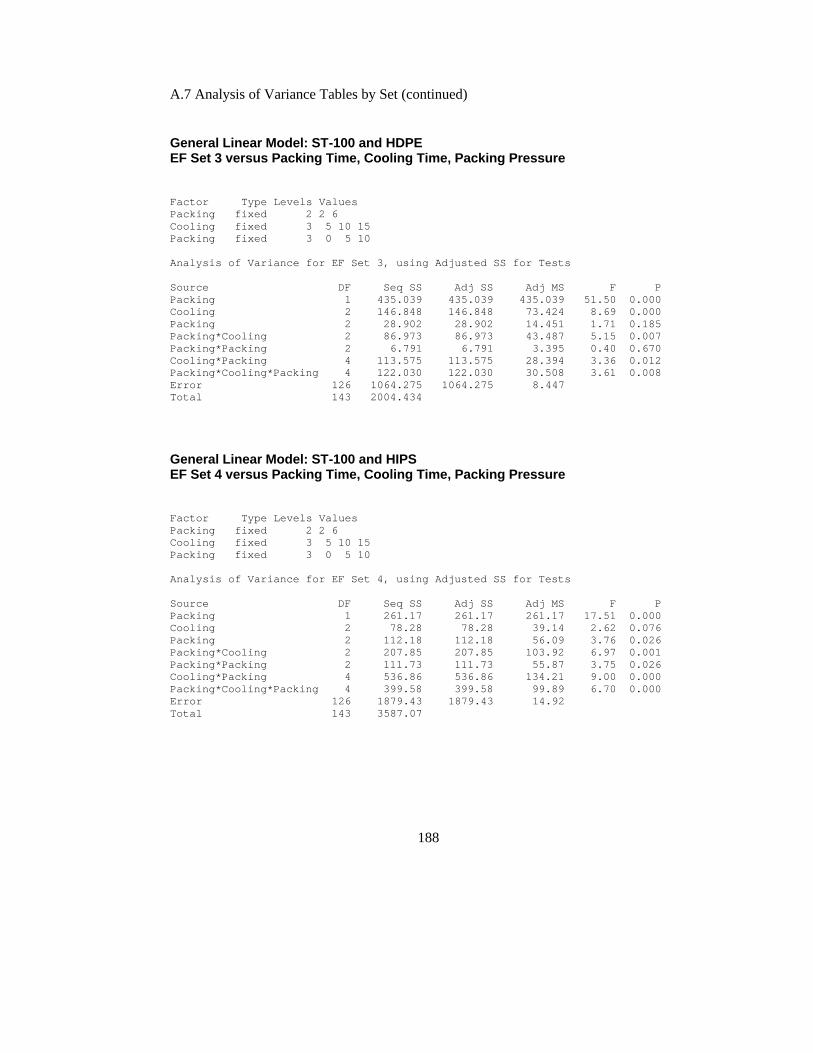
188

A.7 Analysis of Variance Tables by Set (continued)

General Linear Model: ST-100 and HDPE EF Set 3 versus Packing Time, Cooling Time, Packing Pressure Factor Type Levels Values Packing fixed 2 2 6 Cooling fixed 3 5 10 15 Packing fixed 3 0 5 10 Analysis of Variance for EF Set 3, using Adjusted SS for Tests Source DF Seq SS Adj SS Adj MS F P Packing 1 435.039 435.039 435.039 51.50 0.000 Cooling 2 146.848 146.848 73.424 8.69 0.000 Packing 2 28.902 28.902 14.451 1.71 0.185 Packing*Cooling 2 86.973 86.973 43.487 5.15 0.007 Packing*Packing 2 6.791 6.791 3.395 0.40 0.670 Cooling*Packing 4 113.575 113.575 28.394 3.36 0.012 Packing*Cooling*Packing 4 122.030 122.030 30.508 3.61 0.008 Error 126 1064.275 1064.275 8.447 Total 143 2004.434 General Linear Model: ST-100 and HIPS EF Set 4 versus Packing Time, Cooling Time, Packing Pressure Factor Type Levels Values Packing fixed 2 2 6 Cooling fixed 3 5 10 15 Packing fixed 3 0 5 10 Analysis of Variance for EF Set 4, using Adjusted SS for Tests Source DF Seq SS Adj SS Adj MS F P Packing 1 261.17 261.17 261.17 17.51 0.000 Cooling 2 78.28 78.28 39.14 2.62 0.076 Packing 2 112.18 112.18 56.09 3.76 0.026 Packing*Cooling 2 207.85 207.85 103.92 6.97 0.001 Packing*Packing 2 111.73 111.73 55.87 3.75 0.026 Cooling*Packing 4 536.86 536.86 134.21 9.00 0.000 Packing*Cooling*Packing 4 399.58 399.58 99.89 6.70 0.000 Error 126 1879.43 1879.43 14.92 Total 143 3587.07

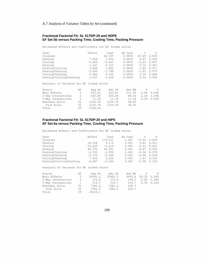
189

A.7 Analysis of Variance Tables by Set (continued)

Fractional Factorial Fit: SL 5170/P-20 and HDPE EF Set 5b versus Packing Time, Cooling Time, Packing Pressure Estimated Effects and Coefficients for EF (coded units) Term Effect Coef SE Coef T P Constant 66.337 0.9830 67.49 0.000 Packing 7.809 3.904 0.9830 3.97 0.000 Cooling -0.485 -0.243 0.9830 -0.25 0.807 Packing 1.447 0.723 0.9830 0.74 0.467 Packing*Cooling 3.666 1.833 0.9830 1.86 0.071 Packing*Packing -3.595 -1.798 0.9830 -1.83 0.077 Cooling*Packing 0.380 0.190 0.9830 0.19 0.848 Packing*Cooling*Packing 1.057 0.529 0.9830 0.54 0.594 Analysis of Variance for EF (coded units) Source DF Seq SS Adj SS Adj MS F P Main Effects 3 633.01 633.01 211.00 5.46 0.004 2-Way Interactions 3 265.08 265.08 88.36 2.29 0.098 3-Way Interactions 1 11.18 11.18 11.18 0.29 0.594 Residual Error 32 1236.78 1236.78 38.65 Pure Error 32 1236.78 1236.78 38.65 Total 39 2146.06 Fractional Factorial Fit: SL 5170/P-20 and HIPS EF Set 6a versus Packing Time, Cooling Time, Packing Pressure Estimated Effects and Coefficients for EF (coded units) Term Effect Coef SE Coef T P Constant 176.511 2.401 73.50 0.000 Packing 18.358 9.179 2.401 3.82 0.001 Cooling -10.220 -5.110 2.401 -2.13 0.041 Packing 40.702 20.351 2.401 8.47 0.000 Packing*Cooling -2.700 -1.350 2.401 -0.56 0.578 Packing*Packing -0.375 -0.188 2.401 -0.08 0.938 Cooling*Packing 7.045 3.523 2.401 1.47 0.152 Packing*Cooling*Packing -4.687 -2.344 2.401 -0.98 0.336 Analysis of Variance for EF (coded units) Source DF Seq SS Adj SS Adj MS F P Main Effects 3 20981.5 20981.5 6993.8 30.32 0.000 2-Way Interactions 3 570.6 570.6 190.2 0.82 0.490 3-Way Interactions 1 219.7 219.7 219.7 0.95 0.336 Residual Error 32 7381.2 7381.2 230.7 Pure Error 32 7381.2 7381.2 230.7 Total 39 29153.1

190

APPENDIX B

MOLD AND CANISTER DRAWINGS

191

B.1 Part Drawing

192

B.2 Mold Insert Drawings

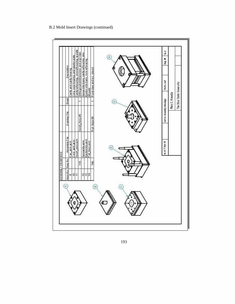
193

B.2 Mold Insert Drawings (continued)

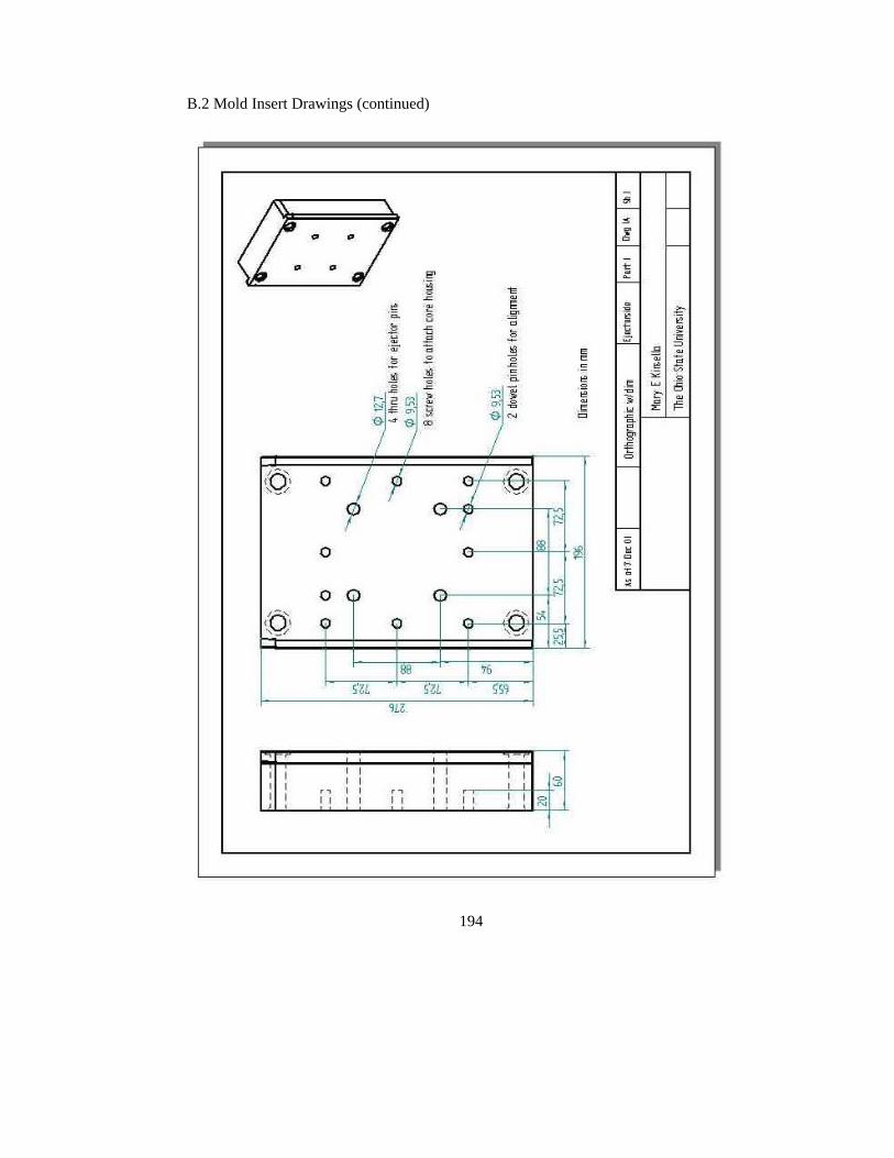
194

B.2 Mold Insert Drawings (continued)

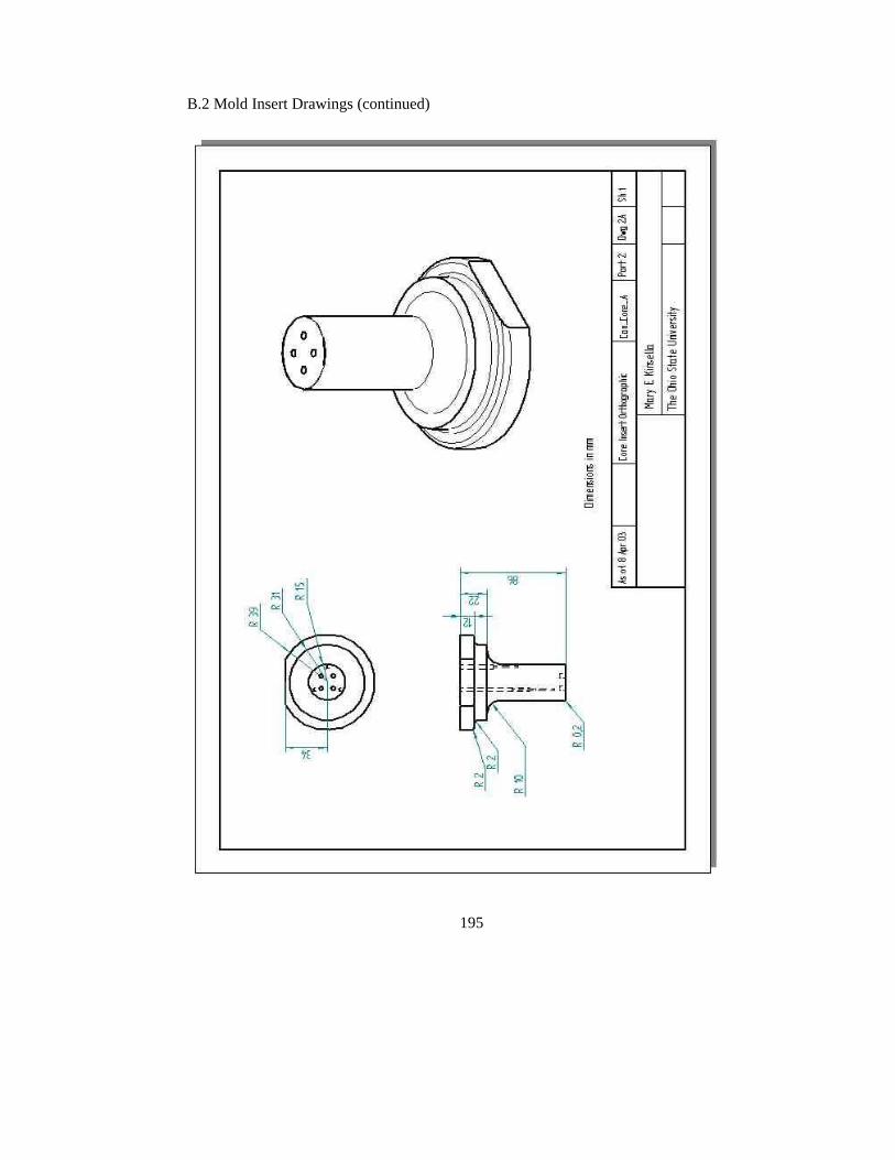
195

B.2 Mold Insert Drawings (continued)

196

B.2 Mold Insert Drawings (continued)

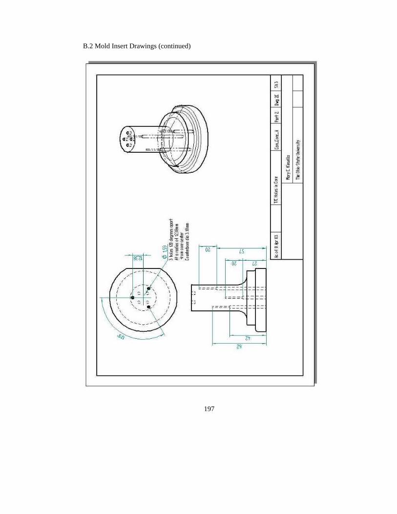
197

B.2 Mold Insert Drawings (continued)

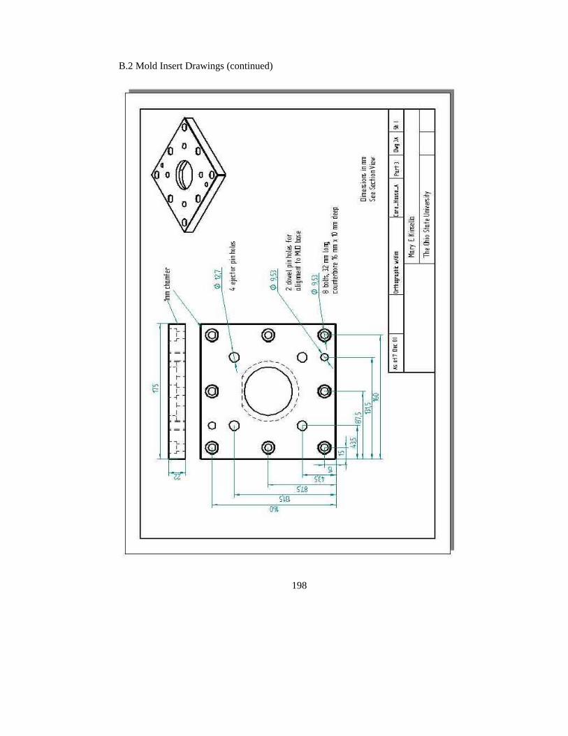
198

B.2 Mold Insert Drawings (continued)

199

B.2 Mold Insert Drawings (continued)

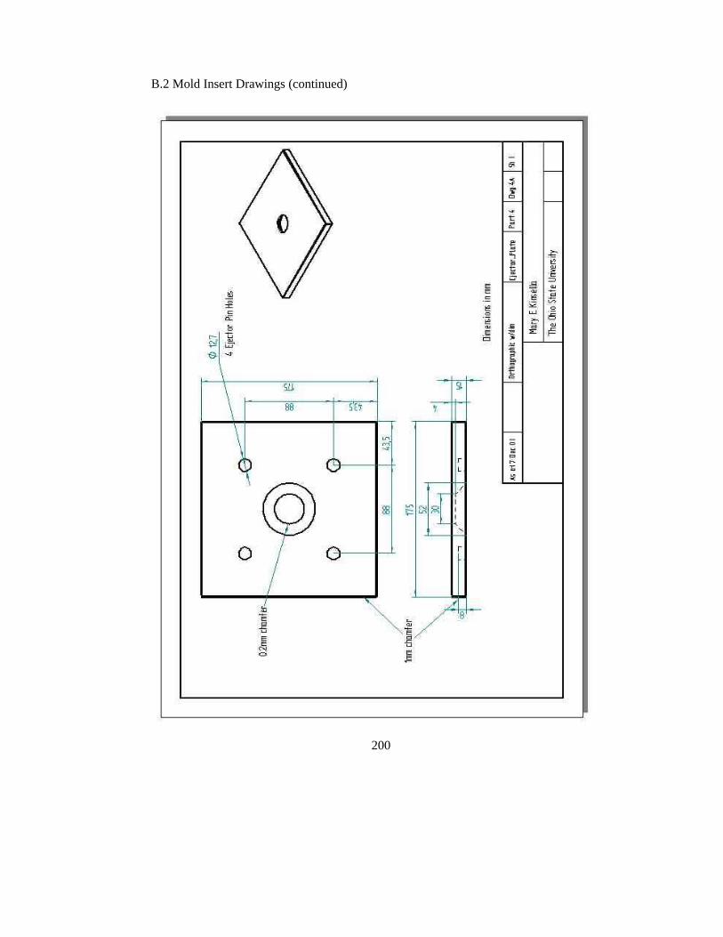
200

B.2 Mold Insert Drawings (continued)

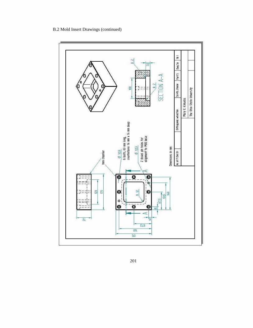
201

B.2 Mold Insert Drawings (continued)

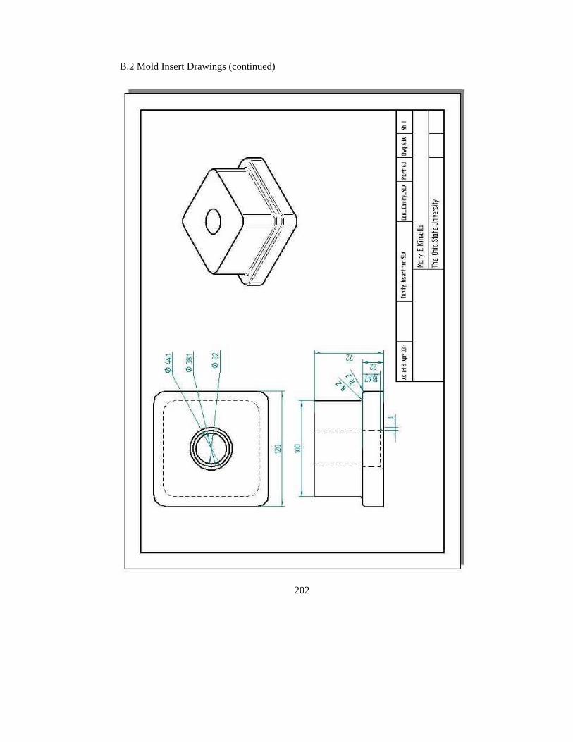
202

B.2 Mold Insert Drawings (continued)

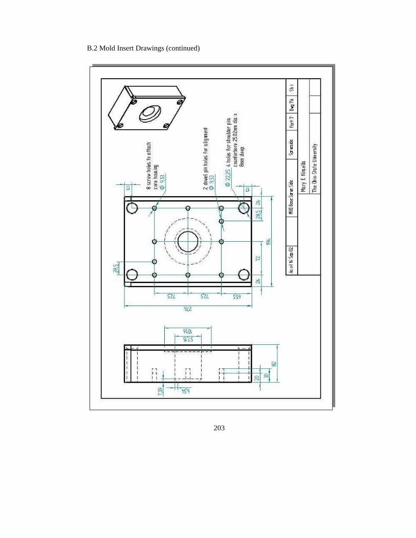
203

B.2 Mold Insert Drawings (continued)

204

B.2 Mold Insert Drawings (continued)

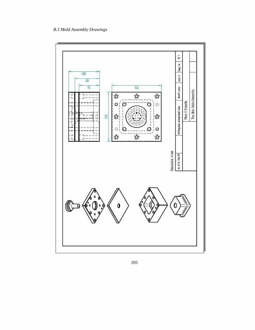
205

B.3 Mold Assembly Drawings

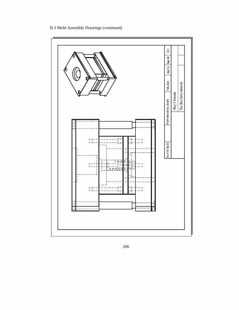
206

B.3 Mold Assembly Drawings (continued)