Module3 direct stiffness- rajesh sir
87
Structural Analysis - III Di t Stiff M th d Direct Stiffness Method Dr. Rajesh K. N. Assistant Professor in Civil Engineering Assistant Professor in Civil Engineering Govt. College of Engineering, Kannur Dept. of CE, GCE Kannur Dr.RajeshKN Dept. of CE, GCE Kannur Dr.RajeshKN 1
-
Upload
shamjith-km -
Category
Engineering
-
view
107 -
download
9
Transcript of Module3 direct stiffness- rajesh sir
Structural Analysis - III
Di t Stiff M th dDirect Stiffness Method
Dr. Rajesh K. N.Assistant Professor in Civil EngineeringAssistant Professor in Civil EngineeringGovt. College of Engineering, Kannur
Dept. of CE, GCE Kannur Dr.RajeshKNDept. of CE, GCE Kannur Dr.RajeshKN
1
Module IIIModule III
Direct stiffness method
• Introduction – element stiffness matrix – rotation transformation
Direct stiffness method
matrix – transformation of displacement and load vectors and stiffness matrix – equivalent nodal forces and load vectors –assembly of stiffness matrix and load vector – determination of assembly of stiffness matrix and load vector determination of nodal displacement and element forces – analysis of plane truss beam and plane frame (with numerical examples) – analysis of grid space frame (without numerical examples) grid – space frame (without numerical examples)
Dept. of CE, GCE Kannur Dr.RajeshKN
2
Introduction
• The formalised stiffness method involves evaluating the displacement transformation matrix CMJ correctlyp y
• Generation of matrix CMJ is not suitable for computer programming
H th l ti f di t tiff th d • Hence the evolution of direct stiffness method
Dept. of CE, GCE Kannur Dr.RajeshKN3
Direct stiffness method
• We need to simplify the assembling process of SJ , the Jassembled structure stiffness matrix
• The key to this is to use member stiffness matrices for actions The key to this is to use member stiffness matrices for actions and displacements at BOTH ends of each member
If b di l d i h f • If member displacements are expressed with reference to global co-ordinates, the process of assembling SJ can be made simplesimple
Dept. of CE, GCE Kannur Dr.RajeshKN
4
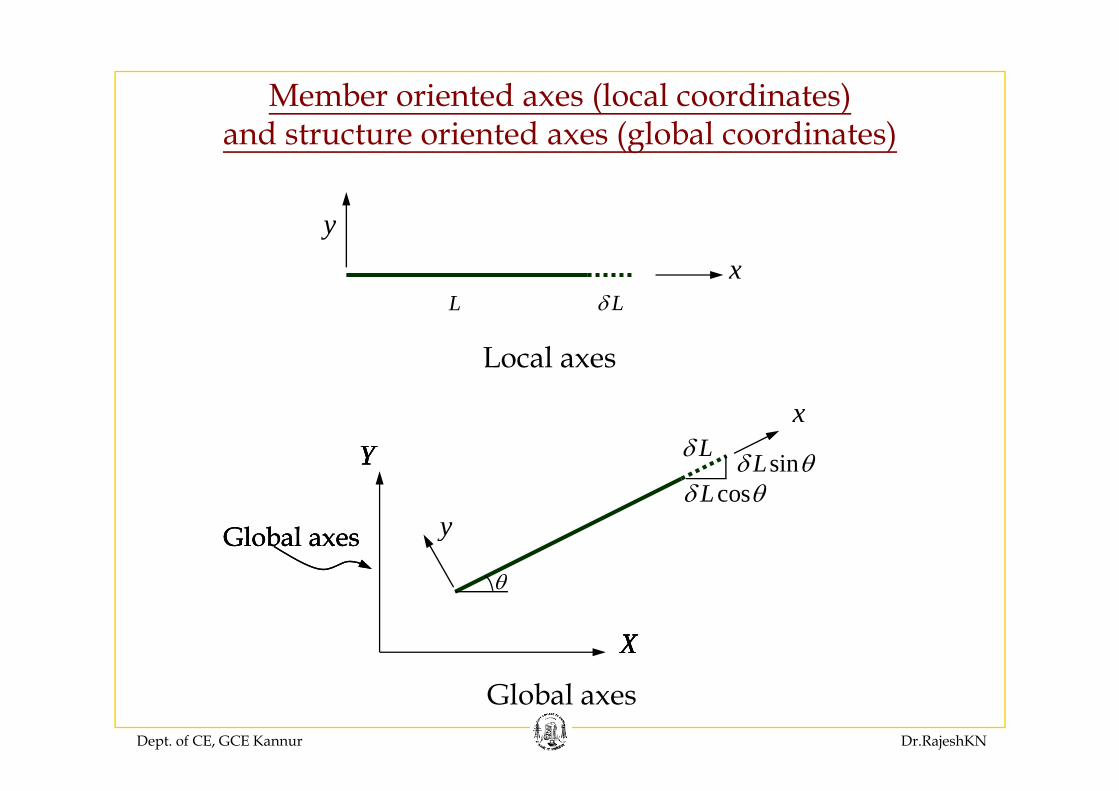
Member oriented axes (local coordinates) d t t i t d ( l b l di t )and structure oriented axes (global coordinates)
Lδx
y
L
Local axes
LδL
Lδ sinLδ θLδ θ
xYYYY
cosLδ θ
θ
Global axes yGlobal axesGlobal axesθ
XXXX
Dept. of CE, GCE Kannur Dr.RajeshKN
Global axes
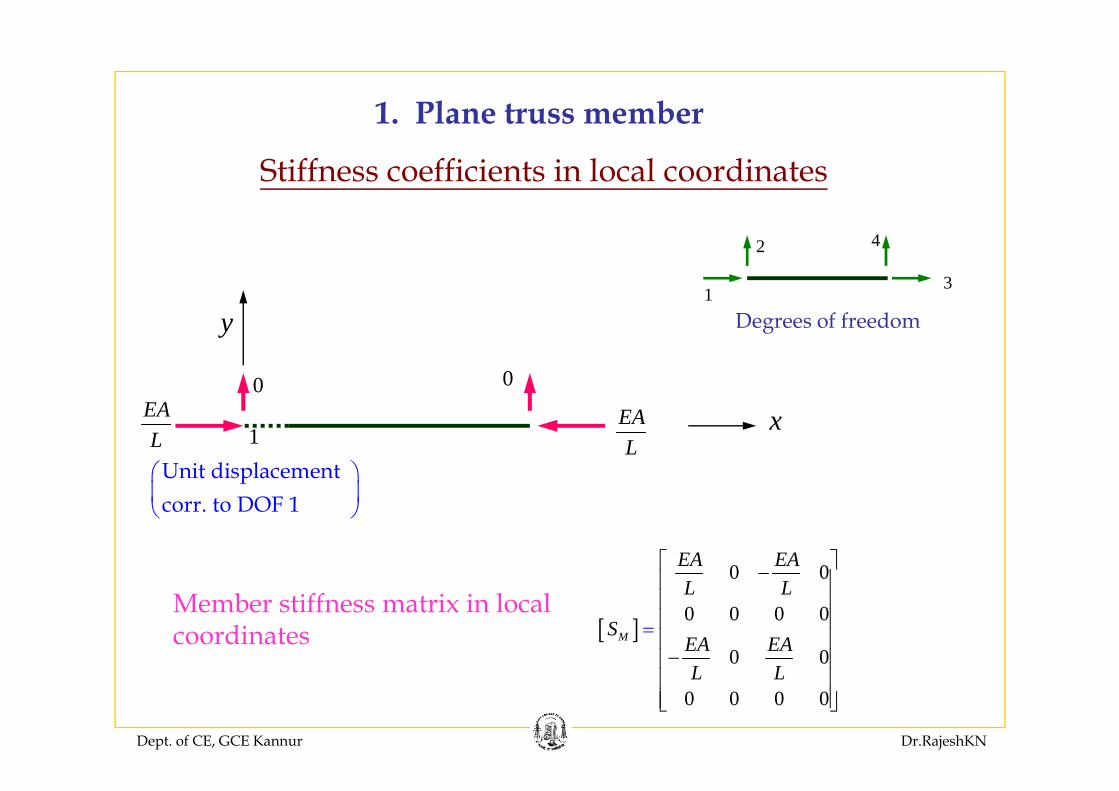
1. Plane truss member
Stiffness coefficients in local coordinates
13
2 4
y
0 0
Degrees of freedom
1
⎛ ⎞⎜ ⎟
Unit displacement
xEAL
EAL
⎜ ⎟⎝ ⎠corr. to DOF 1
0 0EA EA⎡ ⎤−⎢ ⎥
[ ]
0 0
0 0 0 0
0 0M
L L
SEA EA
⎢ ⎥⎢ ⎥⎢ ⎥⎢ ⎥−⎢ ⎥
=Member stiffness matrix in local coordinates
Dept. of CE, GCE Kannur Dr.RajeshKN
0 0 0 0L L⎢ ⎥
⎢⎢⎣ ⎦
⎥⎥
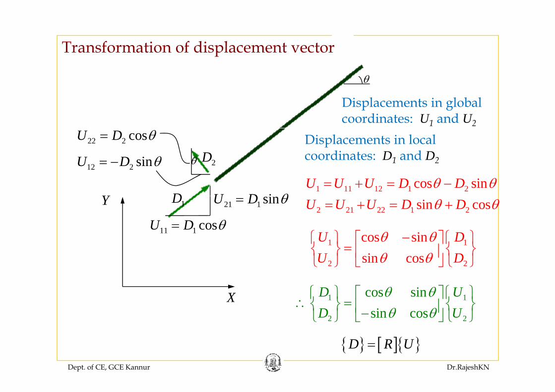
Transformation of displacement vector
θ
Displacements in global
22 2 cosU D θ=
p gcoordinates: U1 and U2
Displacements in local di D d D
2D
DY iU D θ
12 2 sinU D θ= − θ
1 11 12 1 2cos sinU U U D Dθ θ= + = −
coordinates: D1 and D2
1DY
11 1 cosU D θ=
21 1 sinU D θ=2 21 22 1 2sin cosU U U D Dθ θ= + = +
1 1cos sinU Dθ θ−⎧ ⎫ ⎧ ⎫⎡ ⎤
⎧ ⎫ ⎧ ⎫⎡ ⎤
1 1
2 2
cos sinsin cos
U DU D
θ θθ θ
⎧ ⎫ ⎧ ⎫⎡ ⎤=⎨ ⎬ ⎨ ⎬⎢ ⎥⎣ ⎦⎩ ⎭ ⎩ ⎭
X 1 1
2 2
cos sinsin cos
D UD U
θ θθ θ
⎧ ⎫ ⎧ ⎫⎡ ⎤∴ =⎨ ⎬ ⎨ ⎬⎢ ⎥−⎣ ⎦⎩ ⎭ ⎩ ⎭
Dept. of CE, GCE Kannur Dr.RajeshKN
{ } [ ]{ }D R U=
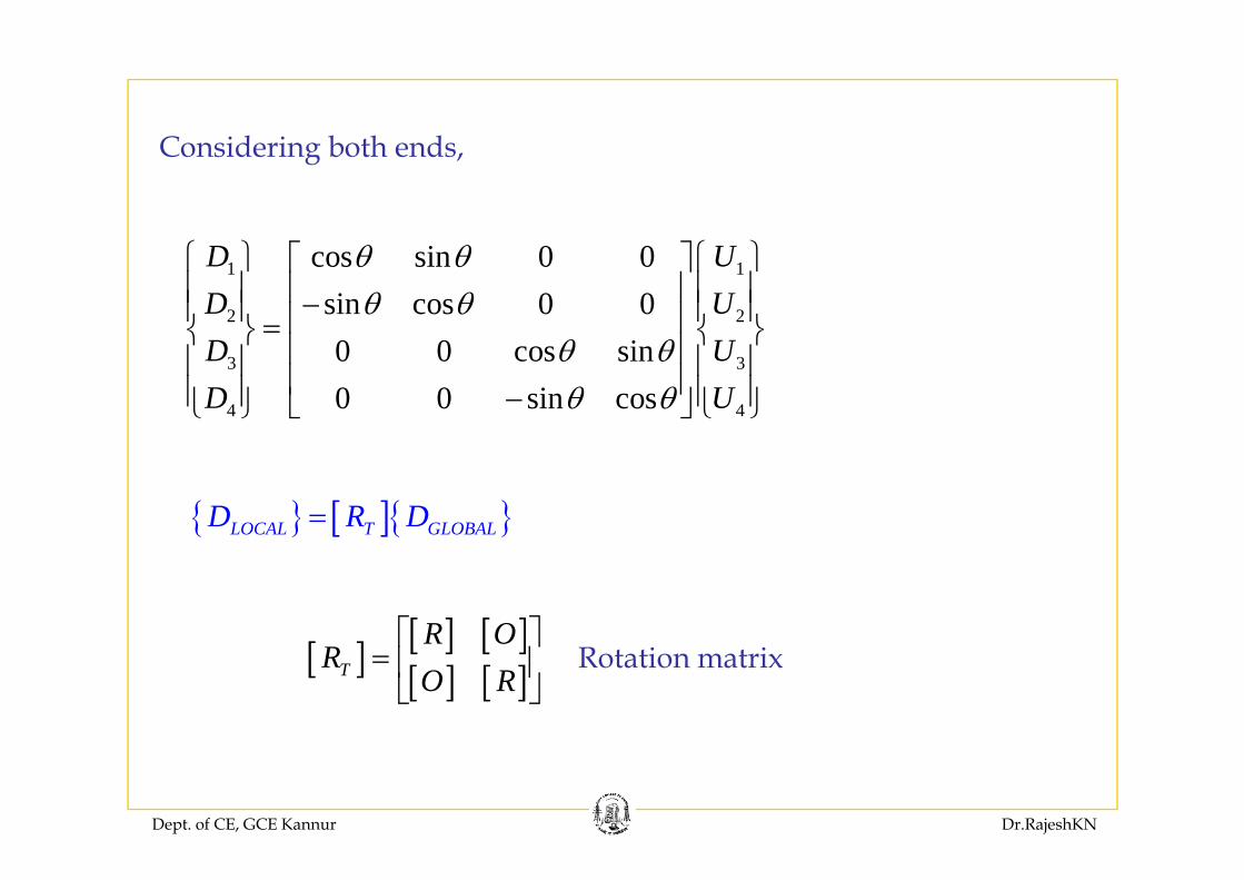
C id i b th d
⎧ ⎫ ⎧ ⎫
Considering both ends,
1 1
2 2
cos sin 0 0sin cos 0 00 0 i
D UD UD U
θ θθ θ
θ θ
⎧ ⎫ ⎧ ⎫⎡ ⎤⎪ ⎪ ⎪ ⎪⎢ ⎥−⎪ ⎪ ⎪ ⎪⎢ ⎥=⎨ ⎬ ⎨ ⎬⎢ ⎥3 3
4 4
0 0 cos sin0 0 sin cos
D UD U
θ θθ θ
⎨ ⎬ ⎨ ⎬⎢ ⎥⎪ ⎪ ⎪ ⎪⎢ ⎥⎪ ⎪ ⎪ ⎪−⎩ ⎭ ⎣ ⎦ ⎩ ⎭
{ } [ ]{ }LOCAL T GLOBALD R D=
[ ] [ ]R O⎡ ⎤[ ] [ ] [ ][ ] [ ]T
R OR
O R⎡ ⎤
= ⎢ ⎥⎣ ⎦
Rotation matrix
Dept. of CE, GCE Kannur Dr.RajeshKN
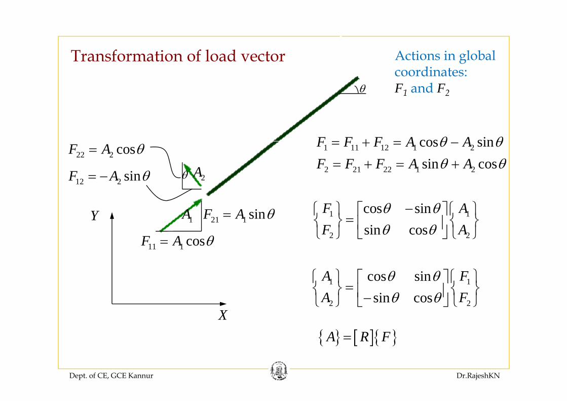
Transformation of load vector Actions in global
θcoordinates: F1 and F2
22 2 cosF A θ= 1 11 12 1 2cos sinF F F A Aθ θ= + = −22 2
12 2 sinF A θ= − θ 2A 2 21 22 1 2sin cosF F F A Aθ θ= + = +
Y
11 1 cosF A θ=
21 1 sinF A θ=1A 1 1
2 2
cos sinsin cos
F AF A
θ θθ θ
−⎧ ⎫ ⎧ ⎫⎡ ⎤=⎨ ⎬ ⎨ ⎬⎢ ⎥⎣ ⎦⎩ ⎭ ⎩ ⎭
11 1
1 1cos sinA Fθ θ⎧ ⎫ ⎧ ⎫⎡ ⎤=⎨ ⎬ ⎨ ⎬⎢ ⎥
X2 2sin cosA Fθ θ⎨ ⎬ ⎨ ⎬⎢ ⎥−⎩ ⎭ ⎣ ⎦ ⎩ ⎭
{ } [ ]{ }A R F=
Dept. of CE, GCE Kannur Dr.RajeshKN
{ } [ ]{ }A R F=
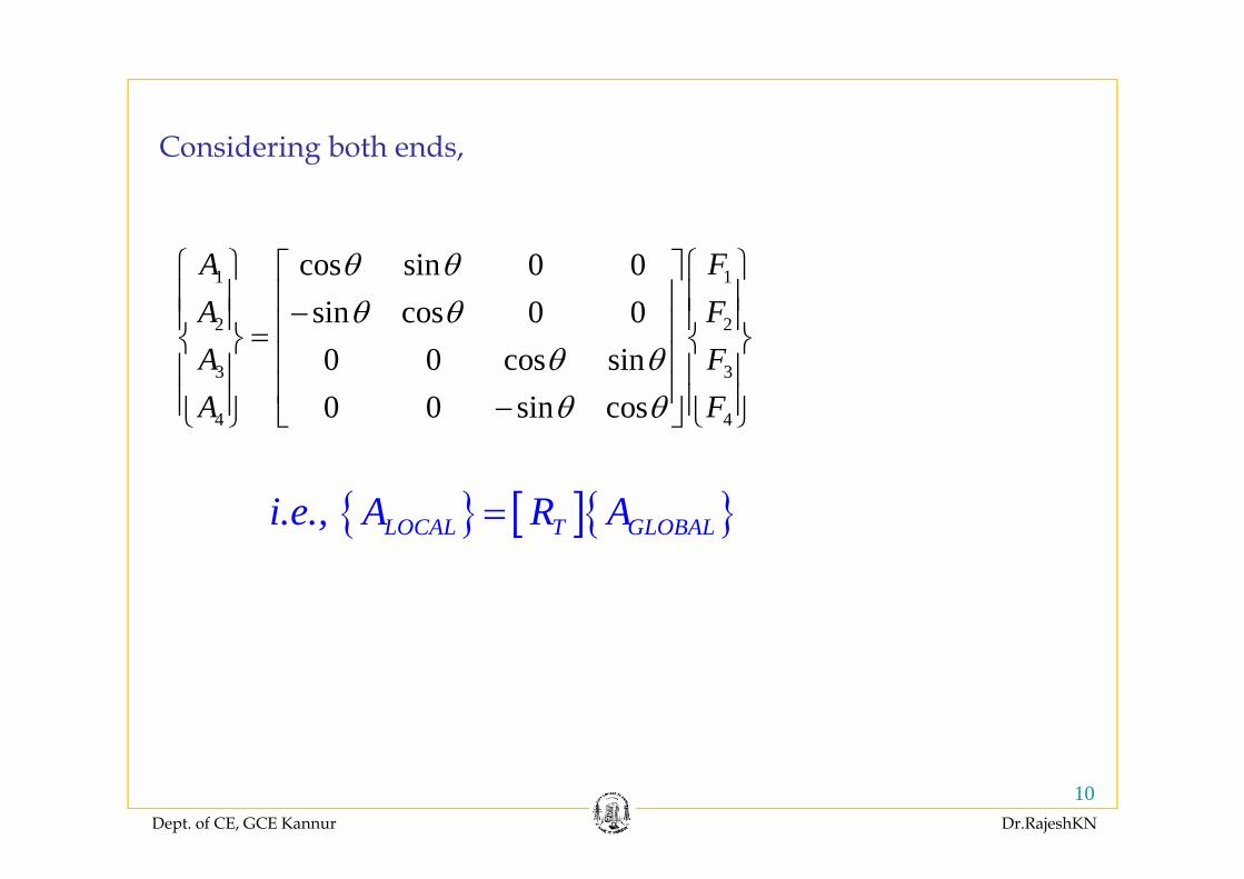
C id i b th dConsidering both ends,
1 1
2 2
cos sin 0 0sin cos 0 0
A FA F
θ θθ θ
⎧ ⎫ ⎧ ⎫⎡ ⎤⎪ ⎪ ⎪ ⎪⎢ ⎥−⎪ ⎪ ⎪ ⎪⎢ ⎥=⎨ ⎬ ⎨ ⎬
3 3
4 4
0 0 cos sin0 0 sin cos
A FA F
θ θθ θ
⎢ ⎥=⎨ ⎬ ⎨ ⎬⎢ ⎥⎪ ⎪ ⎪ ⎪⎢ ⎥⎪ ⎪ ⎪ ⎪−⎩ ⎭ ⎣ ⎦ ⎩ ⎭
{ } [ ]{ }LOCAL T GLOBALi.e., A R A=
Dept. of CE, GCE Kannur Dr.RajeshKN
10
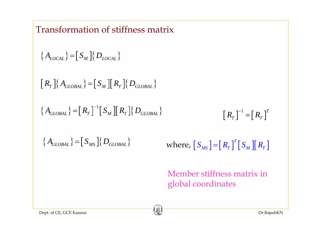
Transformation of stiffness matrix
{ } [ ]{ }LOCAL M LOCALA S D=
[ ]{ } [ ][ ]{ }T GLOBAL M T GLOBALR A S R D=
{ } [ ] [ ][ ]{ }1GLOBAL T M T GLOBALA R S R D−=
[ ]{ } [ ][ ]{ }T GLOBAL M T GLOBAL
[ ] [ ]1 TR R−{ } [ ] [ ][ ]{ }GLOBAL T M T GLOBAL
{ } [ ]{ }A S D
[ ] [ ]T TR R=
{ } [ ]{ }GLOBAL MS GLOBALA S D= [ ] [ ] [ ][ ]TMS T M TS R S R=where,
Member stiffness matrix in global coordinates
Dept. of CE, GCE Kannur Dr.RajeshKN
[ ] [ ] [ ][ ]TS R S R=
T⎡ ⎤ ⎡ ⎤ ⎡ ⎤
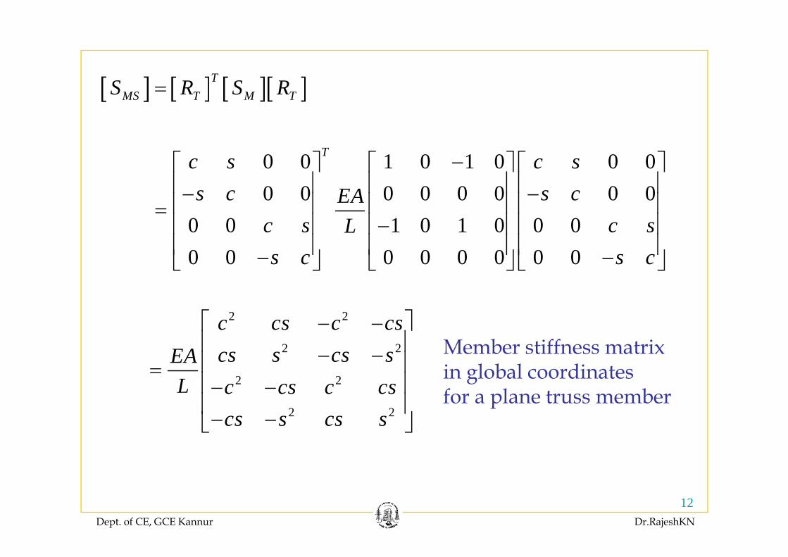
[ ] [ ] [ ][ ]MS T M TS R S R=
0 0 1 0 1 0 0 00 0 0 0 0 0 0 0
Tc s c ss c s cEA
−⎡ ⎤ ⎡ ⎤ ⎡ ⎤⎢ ⎥ ⎢ ⎥ ⎢ ⎥− −⎢ ⎥ ⎢ ⎥ ⎢ ⎥=⎢ ⎥ ⎢ ⎥ ⎢ ⎥0 0 1 0 1 0 0 0
0 0 0 0 0 0 0 0c s c sLs c s c
−⎢ ⎥ ⎢ ⎥ ⎢ ⎥⎢ ⎥ ⎢ ⎥ ⎢ ⎥− −⎣ ⎦ ⎣ ⎦ ⎣ ⎦
2 2c cs c cs⎡ ⎤− −⎢ ⎥ M b tiff t i 2 2
2 2
cs s cs sEAL c cs c cs
⎢ ⎥− −⎢ ⎥=⎢ ⎥− −⎢ ⎥
Member stiffness matrix in global coordinatesfor a plane truss member
2 2cs s cs s⎢ ⎥− −⎣ ⎦
p
Dept. of CE, GCE Kannur Dr.RajeshKN
12
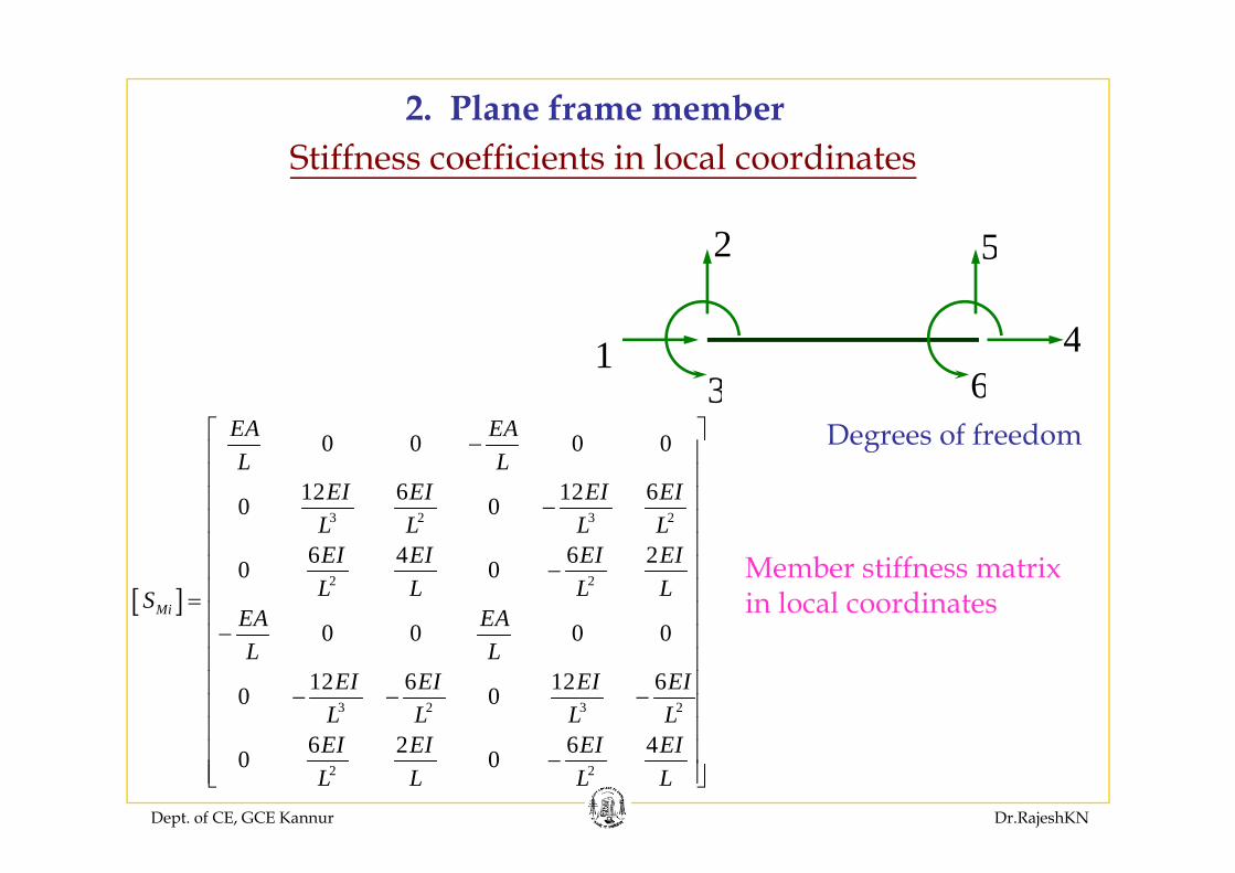
2. Plane frame memberStiffness coefficients in local coordinates
2 52
4
5
Degrees of freedom0 0 0 0EA EA⎡ ⎤
13
46
Degrees of freedom
3 2 3 2
0 0 0 0
12 6 12 60 0
L LEI EI EI EI
L L L L
⎡ ⎤−⎢ ⎥⎢ ⎥⎢ ⎥−⎢ ⎥⎢ ⎥
[ ]2 2
6 4 6 20 0
0 0 0 0Mi
EI EI EI EIL L L LS
EA EA
⎢ ⎥⎢ ⎥−⎢ ⎥=⎢ ⎥−⎢ ⎥
Member stiffness matrix in local coordinates
3 2 3 2
0 0 0 0
12 6 12 60 0
L LEI EI EI EI
L L L L
−⎢ ⎥⎢ ⎥⎢ ⎥− − −⎢ ⎥⎢ ⎥
Dept. of CE, GCE Kannur Dr.RajeshKN
2 2
6 2 6 40 0EI EI EI EIL L L L
⎢ ⎥⎢ ⎥−⎢ ⎥⎣ ⎦
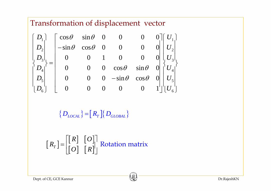
Transformation of displacement vector
1 1
2 2
cos sin 0 0 0 0sin cos 0 0 0 0
D UD U
θ θθ θ
⎧ ⎫ ⎧ ⎫⎡ ⎤⎪ ⎪ ⎪ ⎪⎢ ⎥−⎪ ⎪ ⎪ ⎪⎢ ⎥
3 3
4 4
0 0 1 0 0 00 0 0 cos sin 0
D UD Uθ θ
⎪ ⎪ ⎪ ⎪⎢ ⎥⎪ ⎪ ⎪ ⎪⎢ ⎥
=⎨ ⎬ ⎨ ⎬⎢ ⎥⎪ ⎪ ⎪ ⎪⎢ ⎥⎪ ⎪ ⎪ ⎪⎢ ⎥5 5
6 6
0 0 0 sin cos 00 0 0 0 0 1
D UD U
θ θ⎪ ⎪ ⎪ ⎪⎢ ⎥−⎪ ⎪ ⎪ ⎪⎢ ⎥
⎣ ⎦⎩ ⎭ ⎩ ⎭
{ } [ ]{ }LOCAL T GLOBALD R D=
[ ] [ ]R O⎡ ⎤
{ } [ ]{ }LOCAL T GLOBAL
[ ] [ ] [ ][ ] [ ]T
R OR
O R⎡ ⎤
= ⎢ ⎥⎣ ⎦
Rotation matrix
Dept. of CE, GCE Kannur Dr.RajeshKN
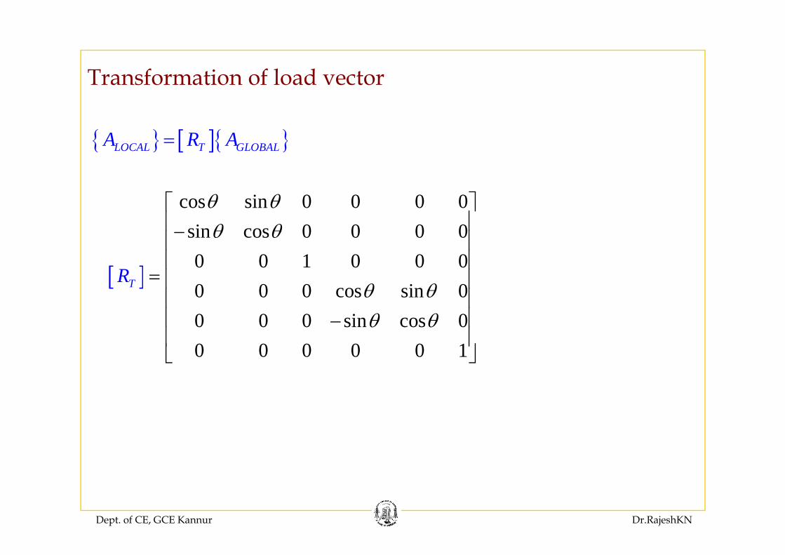
Transformation of load vector
{ } [ ]{ }LOCAL T GLOBALA R A={ } [ ]{ }
cos sin 0 0 0 0θ θ⎡ ⎤⎢ ⎥
[ ]
sin cos 0 0 0 00 0 1 0 0 0
R
θ θ⎢ ⎥−⎢ ⎥⎢ ⎥
= ⎢ ⎥[ ]0 0 0 cos sin 00 0 0 sin cos 0
TRθ θθ θ
= ⎢ ⎥⎢ ⎥⎢ ⎥−⎢ ⎥0 0 0 0 0 1⎢ ⎥⎣ ⎦
Dept. of CE, GCE Kannur Dr.RajeshKN
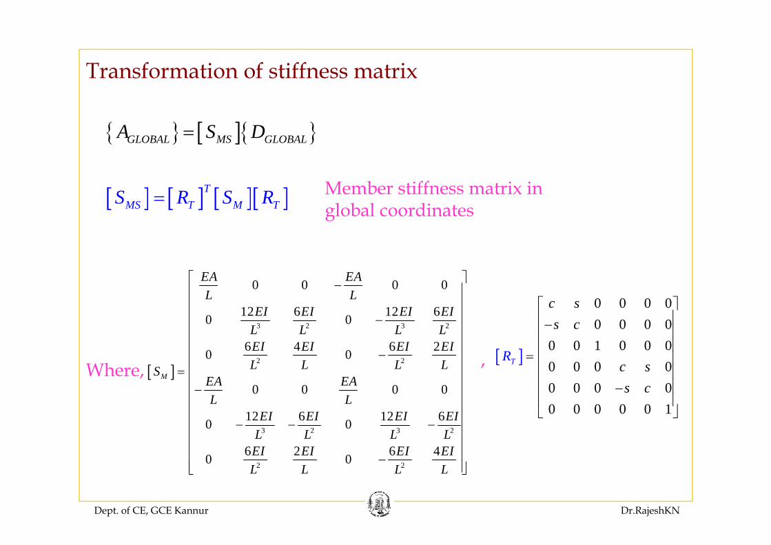
Transformation of stiffness matrix
{ } [ ]{ }GLOBAL MS GLOBALA S D=
[ ] [ ] [ ][ ]TMS T M TS R S R= Member stiffness matrix in
global coordinatesglobal coordinates
EA EA⎡ ⎤
0 0 0 00 0 0 0
c ss c
⎡ ⎤⎢ ⎥−⎢ ⎥3 2 3 2
0 0 0 0
12 6 12 60 0
EA EAL L
EI EI EI EIL L L L
⎡ ⎤−⎢ ⎥⎢ ⎥⎢ ⎥−⎢ ⎥⎢ ⎥
[ ] 0 0 1 0 0 00 0 0 00 0 0 0
T c ss c
R
⎢ ⎥⎢ ⎥
= ⎢ ⎥⎢ ⎥⎢ ⎥−⎢ ⎥
[ ]2 2
6 4 6 20 0
0 0 0 0M
EI EI EI EIL L L LS
EA EAL L
⎢ ⎥⎢ ⎥−⎢ ⎥=⎢ ⎥−⎢ ⎥
Where, ,
0 0 0 0 0 1⎢ ⎥⎣ ⎦
3 2 3 2
12 6 12 60 0
6 2 6 40 0
L LEI EI EI EI
L L L LEI EI EI EI
⎢ ⎥⎢ ⎥⎢ ⎥− − −⎢ ⎥⎢ ⎥⎢ ⎥
Dept. of CE, GCE Kannur Dr.RajeshKN
2 20 0L L L L
⎢ ⎥−⎢ ⎥⎣ ⎦
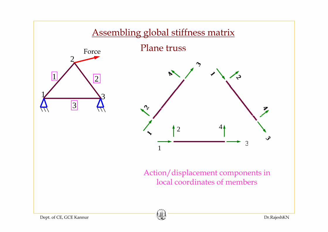
Assembling global stiffness matrixg gPlane truss
2Force
21
331
3
2 4
13
Action/displacement components in local coordinates of members
Dept. of CE, GCE Kannur Dr.RajeshKN
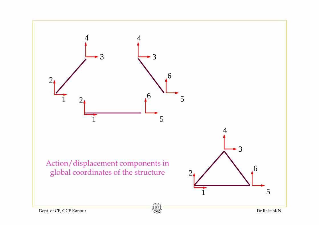
4 4
3
4
3
4
2 6
1 562
514
3
Action/displacement components in 2
5
6Action/displacement components in
global coordinates of the structure
Dept. of CE, GCE Kannur Dr.RajeshKN
1 5
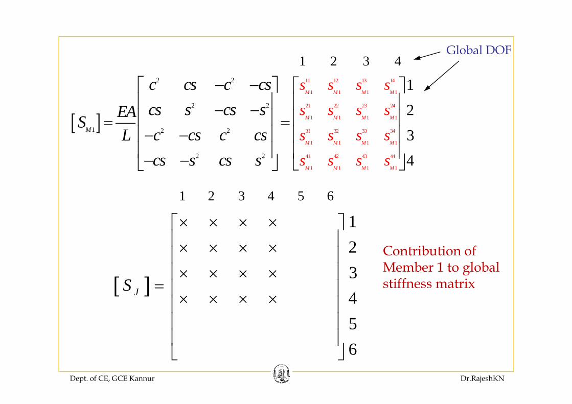
1 2 3 4Global DOF
11 12 13 14
1 1 1 1
21 22 23 24
2 2
2 2
12
M M M Ms s s ss s s s
c cs c cscs s cs sEA
− −⎡ ⎤ ⎡ ⎤⎢ ⎥ ⎢ ⎥− −⎢ ⎥ ⎢ ⎥
1 2 3 4
[ ] 1 1 1 1
31 32 33 34
1 1 1 1
41 42 43 44
1 2 2
2 2
234
M M M M
M M M M
M
s s s ss s s s
cs s cs sEASc cs c csL
− −⎢ ⎥ ⎢ ⎥= =− −⎢ ⎥ ⎢ ⎥⎢ ⎥ ⎢ ⎥
⎣ ⎦⎣ ⎦41 42 43 44
1 1 1 1
2 2 4M M M M
s s s scs s cs s⎢ ⎥ ⎢ ⎥− − ⎣ ⎦⎣ ⎦
1 2 3 4 5 6
12
× × × ×⎡ ⎤⎢ ⎥× × × ×⎢ ⎥ C t ib ti f
[ ]
234JS
× × × ×⎢ ⎥× × × ×⎢ ⎥
= ⎢ ⎥
Contribution of Member 1 to global stiffness matrix[ ]
45
J ⎢ ⎥× × × ×⎢ ⎥⎢ ⎥⎢ ⎥
Dept. of CE, GCE Kannur Dr.RajeshKN
6⎢ ⎥⎣ ⎦
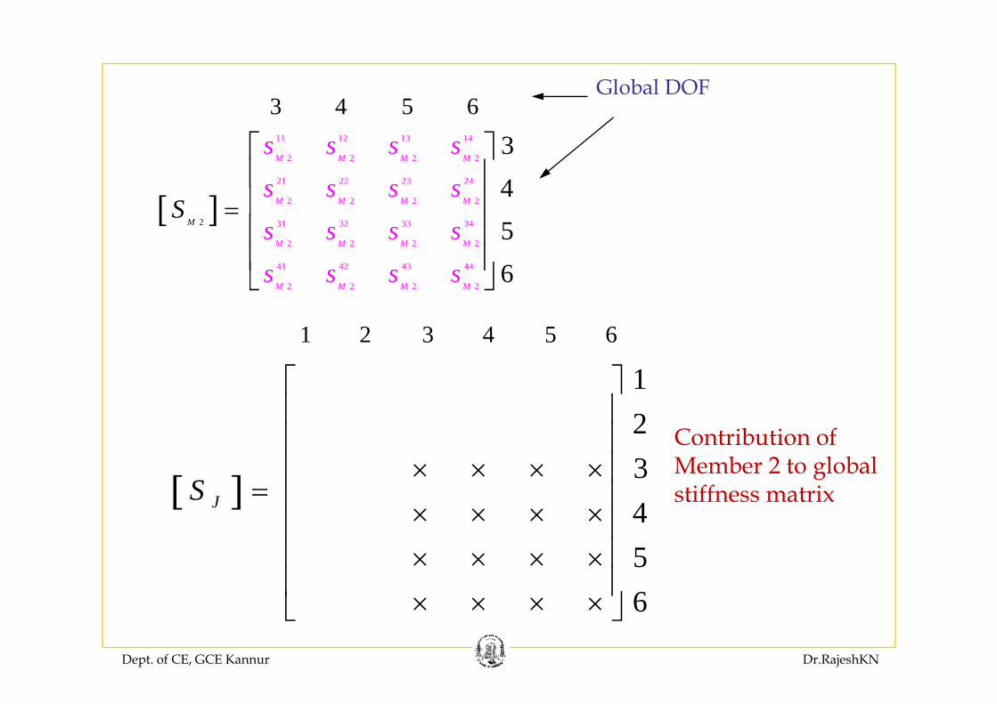
3 4 5 6Global DOF
11 12 13 14
2 2 2 2
21 22 23 24
34
M M M Ms s s ss s s s⎡ ⎤⎢ ⎥⎢ ⎥
3 4 5 6
[ ] 2 2
2
2 2
31 32 33 34
2 2 2 2
41 42 43 44
456
M M M M
M M M
M
M
s s s ss s s ss s s s
S = ⎢ ⎥⎢ ⎥⎢ ⎥⎣ ⎦2 2 2 2
6M M M M
s s s s⎣ ⎦
1 2 3 4 5 6
12
⎡ ⎤⎢ ⎥⎢ ⎥ C t ib ti f
[ ]
234JS
⎢ ⎥× × × ×⎢ ⎥
= ⎢ ⎥× × × ×⎢ ⎥
Contribution of Member 2 to global stiffness matrix
456
× × × ×⎢ ⎥⎢ ⎥× × × ×⎢ ⎥⎣ ⎦
Dept. of CE, GCE Kannur Dr.RajeshKN
6⎢ ⎥× × × ×⎣ ⎦

11 12 13 14 1⎡ ⎤1 2 5 6
Global DOF
[ ]
11 12 13 14
3 3 3 3
21 22 23 24
3 3 3 3
12
M M M M
M M M M
s s s ss s s s
S
⎡ ⎤⎢ ⎥⎢ ⎥[ ] 3 3
3
3 3
31 32 33 34
3 3 3 3
41 42 43 44
56
M M M M
M M M
M
Ms s s s
S = ⎢ ⎥⎢ ⎥⎢ ⎥⎣ ⎦
41 42 43 44
3 3 3 36
M M M Ms s s s⎢ ⎥⎣ ⎦
1 2 3 4 5 6
12
× × × ×⎡ ⎤⎢ ⎥
1 2 3 4 5 6
[ ]
23
JS
⎢ ⎥× × × ×⎢ ⎥⎢ ⎥
= ⎢ ⎥
Contribution of Member 3 to global stiffness matrix[ ]
45
JS ⎢ ⎥⎢ ⎥⎢ ⎥× × × ×⎢ ⎥
stiffness matrix
Dept. of CE, GCE Kannur Dr.RajeshKN
6⎢ ⎥× × × ×⎣ ⎦
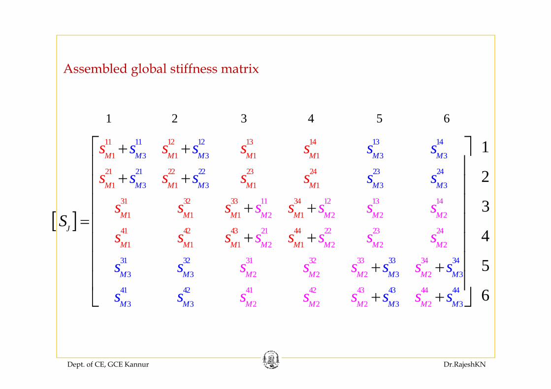
Assembled global stiffness matrix
11 12 13 1411 12 13 14s s s ss s s s+ + 1⎡ ⎤
1 2 3 4 5 6
1 1 1 1
21 22 23 24
1 1 1 1
3 3 3 3
21 22 23 24
3 3 3 3
M M M M
M M M M
M M M M
M M M M
s s s s
s s s s
s s s s
s s s s
+ +
+ +
1
2
⎡ ⎤⎢ ⎥⎢ ⎥⎢ ⎥
[ ]31 32 3 11 12 13 14
2 2 2 2
21 22 23 24
3 34
1 1 1 1
41 42 43 44
M M M MM M M M
J
s s s s
s s s s
s s s s
sS
ss s
+ +=
+ +
3
4
⎢ ⎥⎢ ⎥⎢ ⎥
31 3
2 2 2 2
31 32 33
1 1
2
2
1 1
23 3 32
M M M M
M MM M
M M M M
MMs s
s s s s
s s
s s
s
s s
s
+ +
+ 34
2
33 34
3
4
5MM ss +
⎢ ⎥⎢ ⎥⎢ ⎥41 42 43 44
2
41 42 43 44
3 2 23 32 36
M M M MM M M Ms s s ss s s s+ +⎢ ⎥⎣ ⎦
Dept. of CE, GCE Kannur Dr.RajeshKN
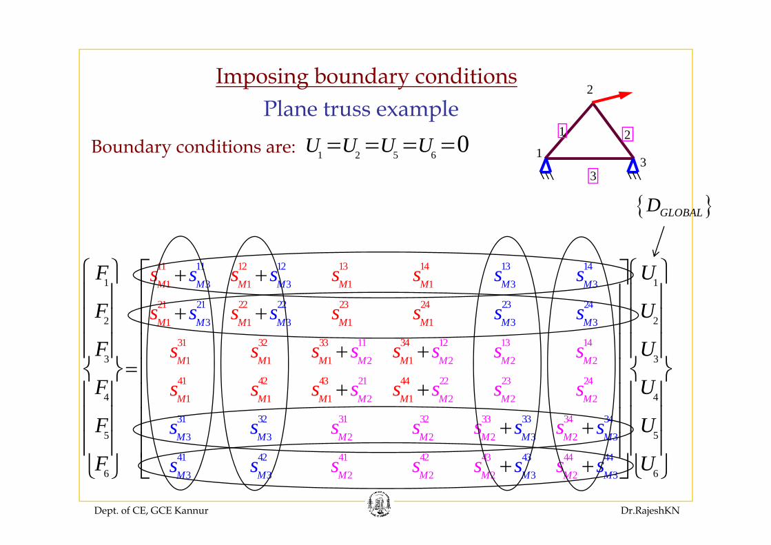
Imposing boundary conditions2
p g yPlane truss example
21
1
2
0U U U U= = = =Boundary conditions are:3
311 2 5 6 0U U U UBoundary conditions are:
{ }GLOBALD
11 12 13 1411 12 13 14s s s ssF s s s+ +⎧ ⎫ U⎧ ⎫⎡ ⎤
{ }GLOBALD
3 3 3 31 1 1 1
2 21 221 22 23 24
1 1 1 1
23 24
1
2 3 3 3 3
M MM M M M
M M M M
M M
M M M M
s s s s
s s s s
sF
F
s s s
s s s s
+ +
+ +
⎧ ⎫⎪ ⎪⎪ ⎪⎪ ⎪
1
2
U
U
⎧ ⎫⎡ ⎤⎪ ⎪⎢ ⎥⎪ ⎪⎢ ⎥⎪ ⎪⎢ ⎥11 12 13 14
2 2 2 2
21 22 23 24
2
31 32 33 34
1 1 1 1
41 42 43 44
1
3
1 1 1 24 2 2
M M M M M M M
M M M
M
M M M M M
s s s s
s s s
s s s s
s s s s
F
F s
+ +=
+ +
⎪ ⎪⎨ ⎬⎪ ⎪ 4
3U
U
⎪ ⎪⎢ ⎥⎨ ⎬⎢ ⎥⎪ ⎪⎢ ⎥21 1 1 1 24
5
2 2M M MM M M M M
F
F
s⎪ ⎪⎪ ⎪⎪ ⎪⎩ ⎭
31 32 33 34
2 2 2 2
41 42 43 44
31 32 33 34
3 3 3 3
41 42 43 44
4
5M M M MM M M Ms ss s s s s U
U
+ +⎪ ⎪⎢ ⎥⎪ ⎪⎢ ⎥⎪ ⎪⎢ ⎥
⎣ ⎦⎩ ⎭Dept. of CE, GCE Kannur Dr.RajeshKN
6F⎩ ⎭41 42 43 44
2 2 2 2
41 42 43 44
3 3 3 3 6M MM M M MM Mss s s s ss s U+ +⎣ ⎦⎩ ⎭
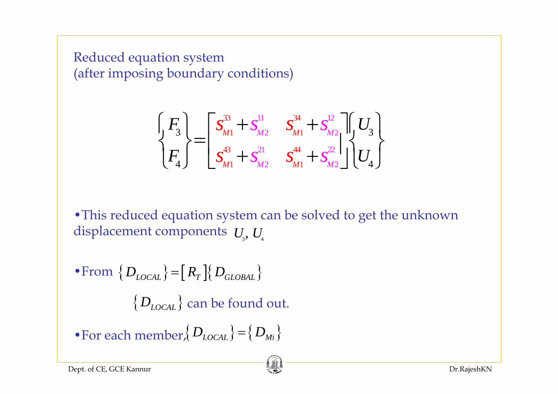
Reduced equation system q y(after imposing boundary conditions)
33 34
1 1
43 44
11 12
2 2
21 22
3 3MM M MF U
F U
s ss s+ +⎧ ⎫ ⎧ ⎫⎡ ⎤=⎨ ⎬ ⎨ ⎬⎢ ⎥+ +⎩ ⎭ ⎣ ⎦⎩ ⎭1 2 1 24 4M MM M
F Us sss⎢ ⎥+ +⎩ ⎭ ⎣ ⎦⎩ ⎭
•This reduced equation system can be solved to get the unknown displacement components
3 4,U U
{ } [ ]{ }LOCAL T GLOBALD R D=•From
{ }LOCALD can be found out.
{ } { }D D=F h b
Dept. of CE, GCE Kannur Dr.RajeshKN
{ } { }LOCAL MiD D=•For each member,

{ } { } [ ]{ }A A S D{ } { } [ ]{ }Mi MLi Mi MiA A S D= +Member end actions
Where,
Fixed end actions on the member, { }MLiA
Member stiffness matrix, [ ]MiS
[ ]
in local coordinates
Displacement components of the member, [ ]MiD
{ } { } [ ]{ }LOCAL T GLOBALMi D R DD ==As we know,
{ } { } [ ][ ]{ }i i iM ML M i iT GLOBALA A S R D∴ = +
Dept. of CE, GCE Kannur Dr.RajeshKN
25
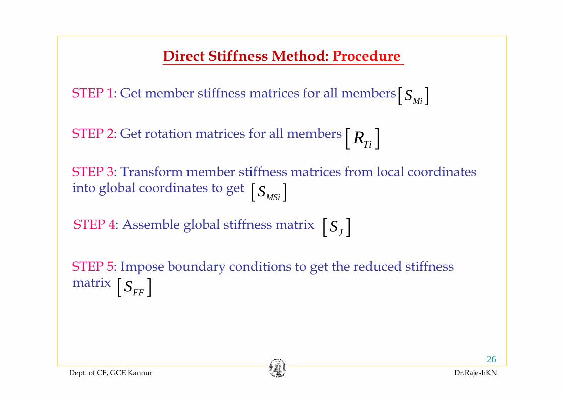
Direct Stiffness Method: Procedure
STEP 1: Get member stiffness matrices for all members [ ]MiS
STEP 2: Get rotation matrices for all members [ ]TiR
STEP 3: Transform member stiffness matrices from local coordinates into global coordinates to get [ ]MSiS[ ]MSi
STEP 4: Assemble global stiffness matrix [ ]JS
STEP 5: Impose boundary conditions to get the reduced stiffness matrix [ ]S[ ]FFS
Dept. of CE, GCE Kannur Dr.RajeshKN
26
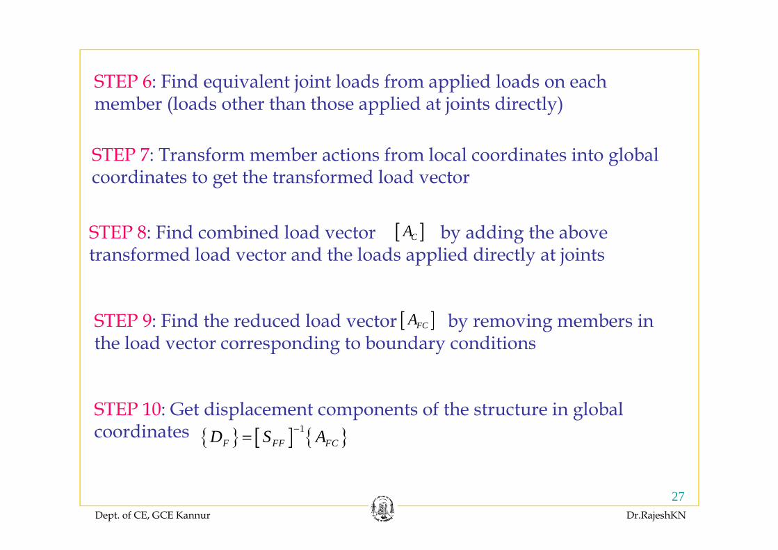
STEP 6: Find equivalent joint loads from applied loads on each q j ppmember (loads other than those applied at joints directly)
STEP 7 T f b ti f l l di t i t l b l STEP 7: Transform member actions from local coordinates into global coordinates to get the transformed load vector
STEP 8: Find combined load vector by adding the above transformed load vector and the loads applied directly at joints
[ ]CA
STEP 9: Find the reduced load vector by removing members in h l d di b d di i
[ ]FCAthe load vector corresponding to boundary conditions
STEP 10: Get displacement components of the structure in global coordinates { } [ ] { }1
F FF FCD S A−=
Dept. of CE, GCE Kannur Dr.RajeshKN
27
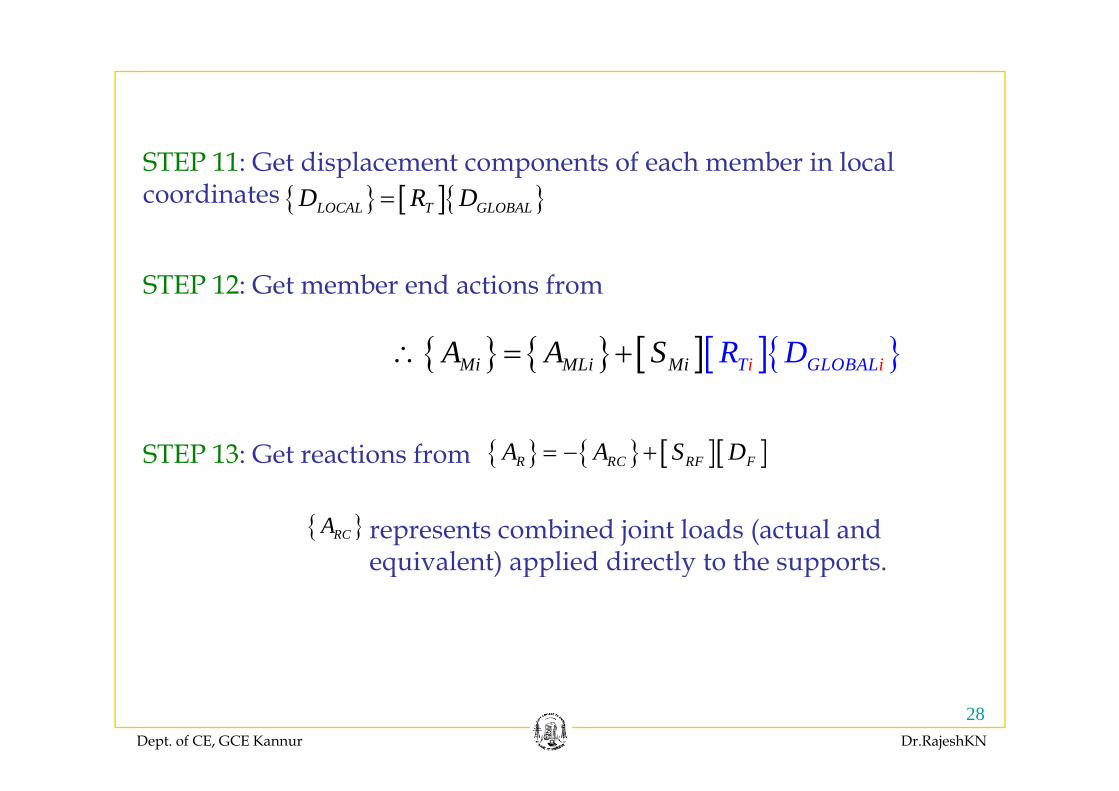
{ } [ ]{ }LOCAL T GLOBALD R D=STEP 11: Get displacement components of each member in local coordinates
STEP 12: Get member end actions from
{ } { } [ ][ ]{ }Mi MLi Mi iT GLOB iALR DA A S∴ = +
{ } { } [ ][ ]R RC RF FA A S D= − +STEP 13: Get reactions from
{ }RCA represents combined joint loads (actual and equivalent) applied directly to the supports.q ) pp y pp
Dept. of CE, GCE Kannur Dr.RajeshKN
28
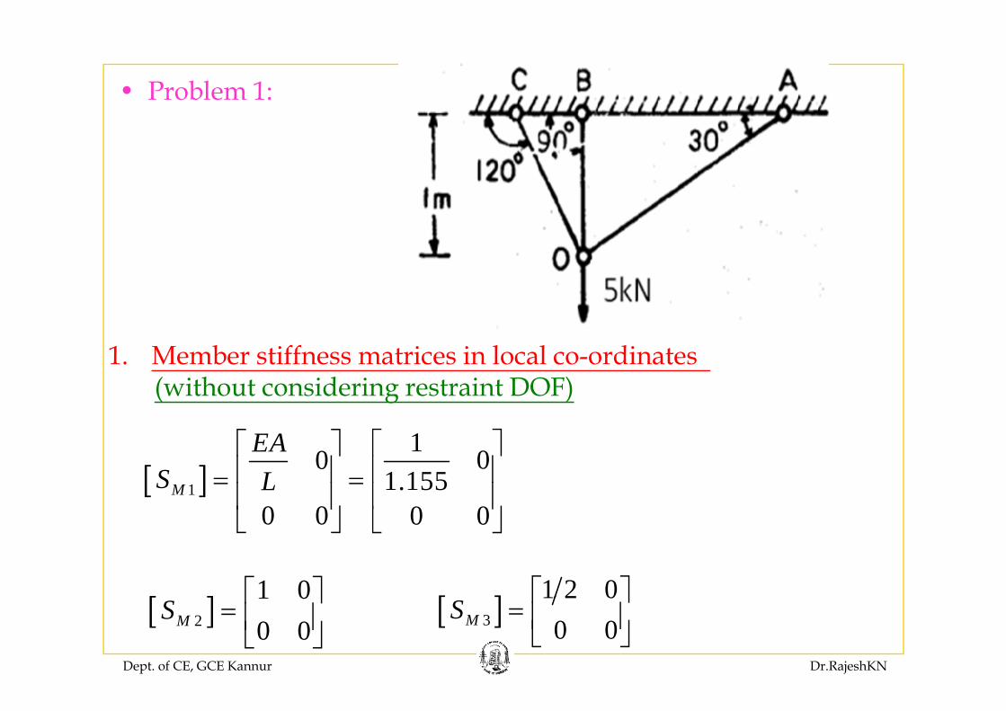
• Problem 1:
1 Member stiffness matrices in local co ordinates
1EA ⎡ ⎤⎡ ⎤
1. Member stiffness matrices in local co-ordinates (without considering restraint DOF)
[ ]1
1 001.155
0 0 0 0M
EAS L
⎡ ⎤⎡ ⎤⎢ ⎥⎢ ⎥= =⎢ ⎥⎢ ⎥
⎣ ⎦ ⎣ ⎦0 0 0 0⎣ ⎦ ⎣ ⎦
[ ] 1 0⎡ ⎤ [ ] 1 2 0⎡ ⎤
Dept. of CE, GCE Kannur Dr.RajeshKN
[ ]2
1 00 0MS ⎡ ⎤
= ⎢ ⎥⎣ ⎦
[ ]3
1 2 00 0MS ⎡ ⎤
= ⎢ ⎥⎣ ⎦
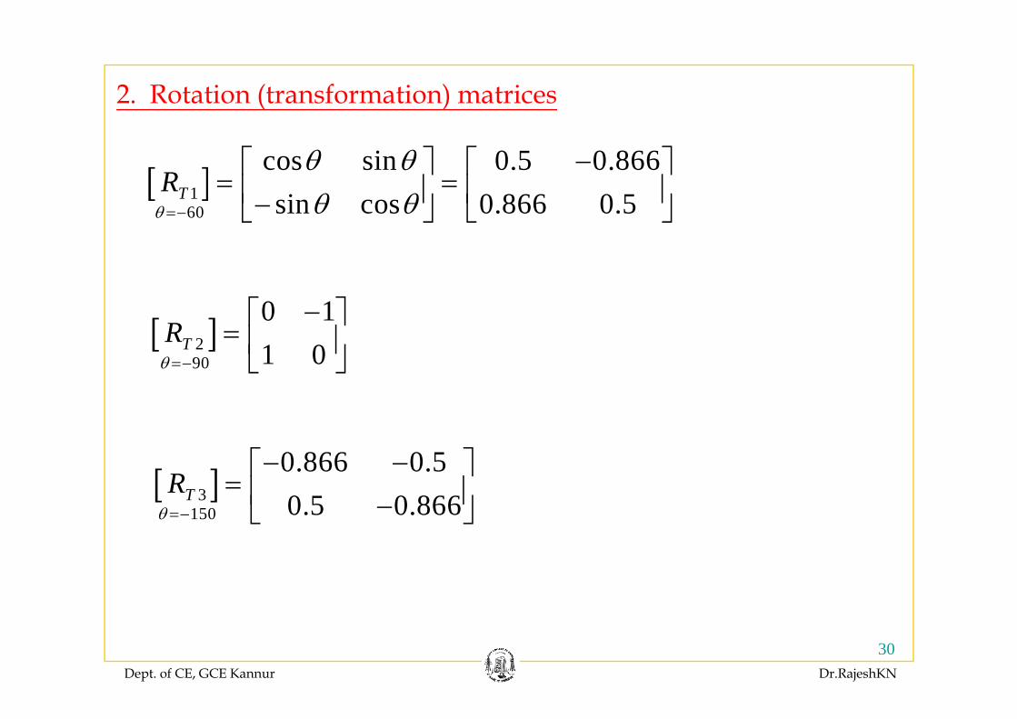
2. Rotation (transformation) matrices
[ ]1
cos sin 0.5 0.866i 0 866 0 5TRθ θθ θ
−⎡ ⎤ ⎡ ⎤= =⎢ ⎥ ⎢ ⎥⎣ ⎦ ⎣ ⎦
[ ]160 sin cos 0.866 0.5T
θ θ θ=−⎢ ⎥ ⎢ ⎥−⎣ ⎦ ⎣ ⎦
[ ]290
0 11 0TR
θ
−⎡ ⎤= ⎢ ⎥⎣ ⎦90 1 0θ =− ⎣ ⎦
[ ]3150
0.866 0.50.5 0.866TR
θ =−
− −⎡ ⎤= ⎢ ⎥−⎣ ⎦⎣ ⎦
Dept. of CE, GCE Kannur Dr.RajeshKN
30
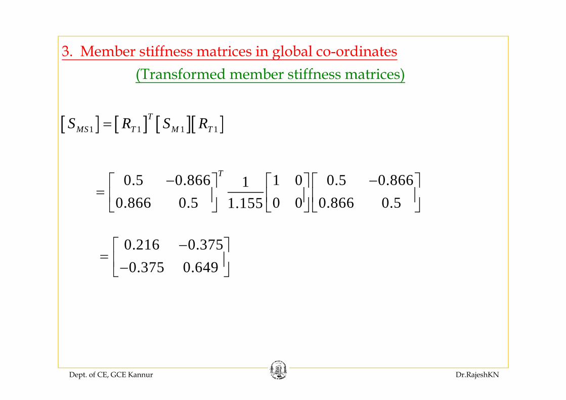
3. Member stiffness matrices in global co-ordinates(Transformed member stiffness matrices)
[ ] [ ] [ ][ ]1 1 1 1T
MS T M TS R S R=
0.5 0.866 1 0 0.5 0.86610 866 0 5 0 0 0 866 0 51 155
T− −⎡ ⎤ ⎡ ⎤ ⎡ ⎤= ⎢ ⎥ ⎢ ⎥ ⎢ ⎥⎣ ⎦ ⎣ ⎦ ⎣ ⎦0.866 0.5 0 0 0.866 0.51.155⎢ ⎥ ⎢ ⎥ ⎢ ⎥⎣ ⎦ ⎣ ⎦ ⎣ ⎦
0 216 0 375−⎡ ⎤0.216 0.3750.375 0.649
−⎡ ⎤= ⎢ ⎥−⎣ ⎦
Dept. of CE, GCE Kannur Dr.RajeshKN
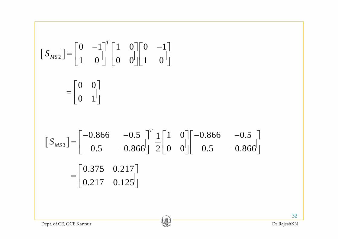
[ ]2
0 1 1 0 0 11 0 0 0 1 0
T
MSS− −⎡ ⎤ ⎡ ⎤ ⎡ ⎤
= ⎢ ⎥ ⎢ ⎥ ⎢ ⎥⎣ ⎦ ⎣ ⎦ ⎣ ⎦⎣ ⎦ ⎣ ⎦ ⎣ ⎦
0 0⎡ ⎤= ⎢ ⎥0 1= ⎢ ⎥⎣ ⎦
[ ]3
0.866 0.5 1 0 0.866 0.510 5 0 866 0 0 0 5 0 8662
T
MSS− − − −⎡ ⎤ ⎡ ⎤ ⎡ ⎤
= ⎢ ⎥ ⎢ ⎥ ⎢ ⎥⎣ ⎦ ⎣ ⎦ ⎣ ⎦
[ ]3 0.5 0.866 0 0 0.5 0.8662MS ⎢ ⎥ ⎢ ⎥ ⎢ ⎥− −⎣ ⎦ ⎣ ⎦ ⎣ ⎦
0.375 0.217⎡ ⎤⎢ ⎥0.217 0.125
= ⎢ ⎥⎣ ⎦
Dept. of CE, GCE Kannur Dr.RajeshKN
32
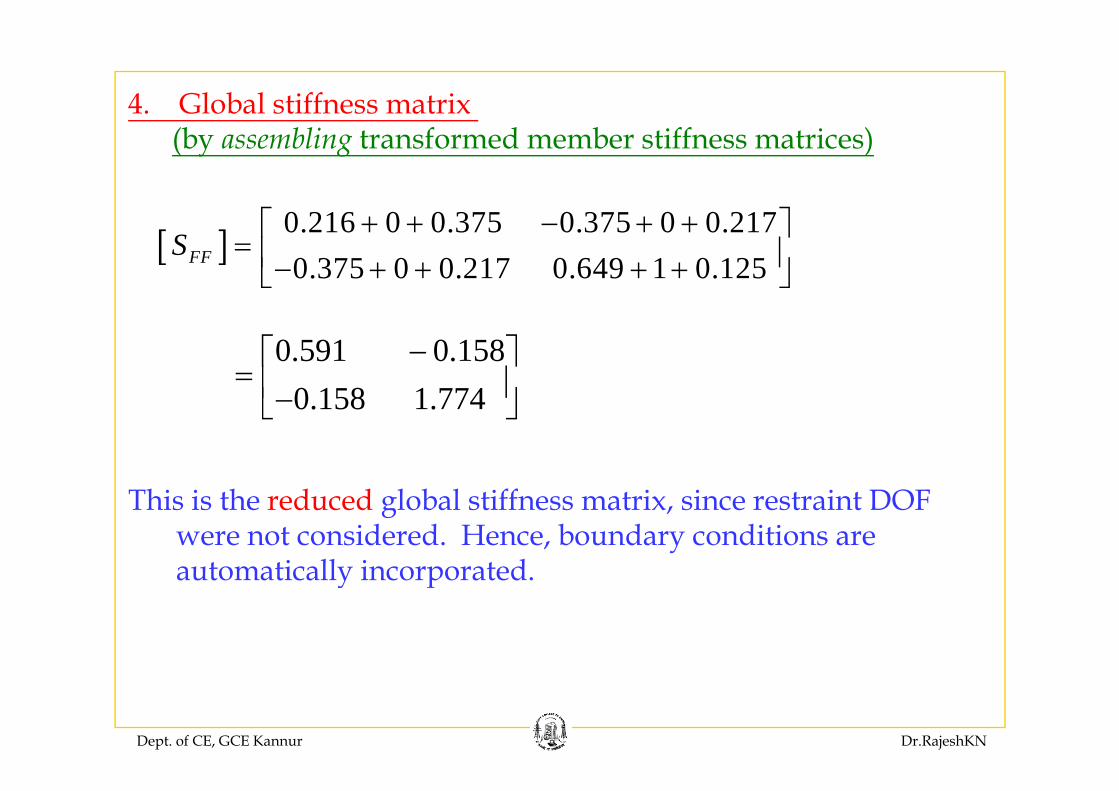
4. Global stiffness matrix
0 216 0 0 375 0 375 0 0 217⎡ ⎤
(by assembling transformed member stiffness matrices)
[ ] 0.216 0 0.375 0.375 0 0.2170.375 0 0.217 0.649 1 0.125FFS
+ + − + +⎡ ⎤= ⎢ ⎥− + + + +⎣ ⎦
0.591 0.1580 158 1 774
−⎡ ⎤= ⎢ ⎥⎣ ⎦0.158 1.774 ⎢ ⎥−⎣ ⎦
This is the reduced global stiffness matrix, since restraint DOF were not considered. Hence, boundary conditions are automatically incorporated automatically incorporated.
Dept. of CE, GCE Kannur Dr.RajeshKN
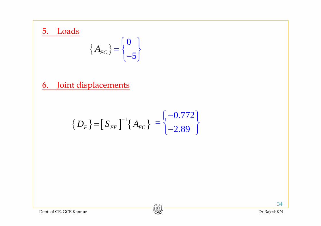
5. Loads
{ }0
5FCA ⎧ ⎫= ⎨ ⎬−⎩ ⎭
6. Joint displacements6. Joint displacements
0 772⎧ ⎫{ } [ ] { }1
F FF FCD S A−=0.7722.89
−⎧ ⎫= ⎨ ⎬−⎩ ⎭
Dept. of CE, GCE Kannur Dr.RajeshKN
34
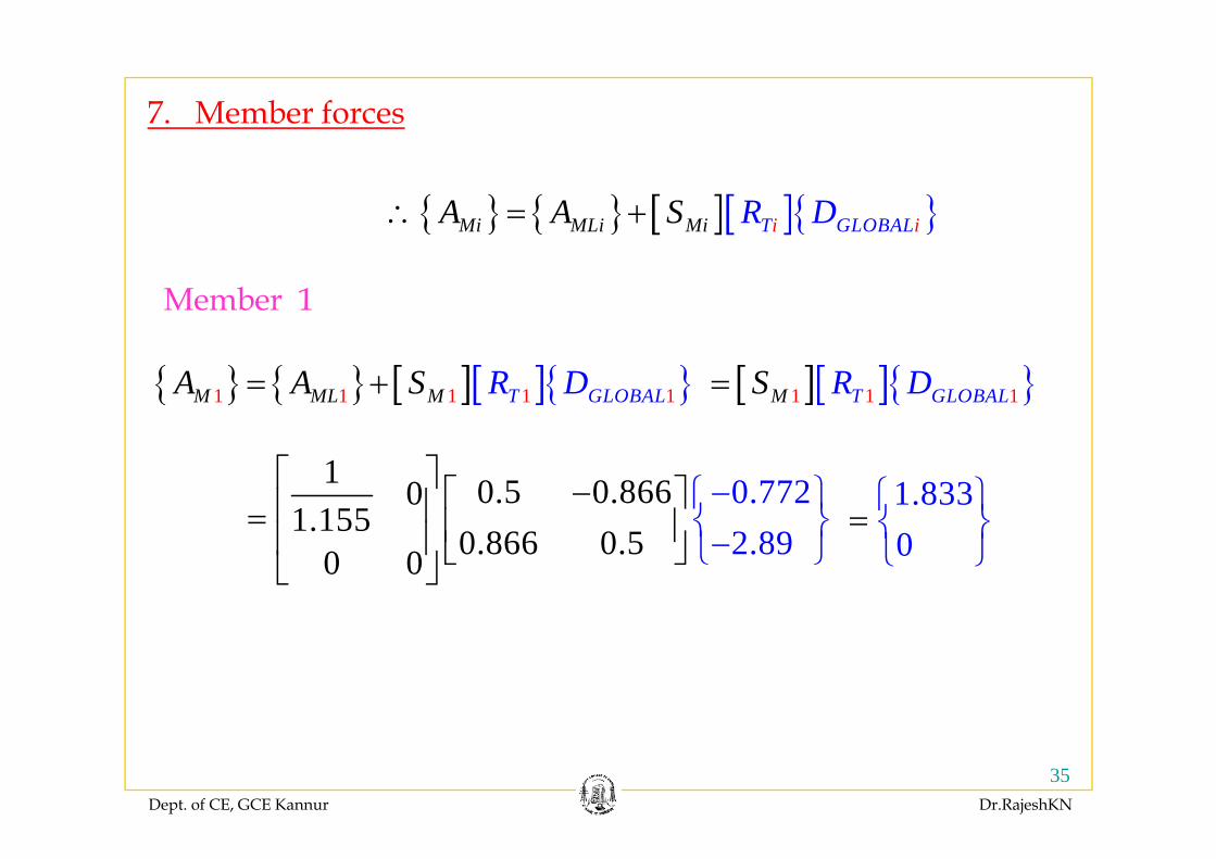
7. Member forces
{ } { } [ ][ ]{ }Mi MLi Mi iT GLOB iALR DA A S∴ = +
Member 1
{ } { } [ ][ ]{ }
{ } { } [ ][ ]{ }1 1 1 1 1TM M G LM L BAL OR DA A S= + [ ][ ]{ }1 1 1T GLOBALM R DS=
1 0.5 0.86601 155
0.772⎡ ⎤ −⎡ ⎤⎢ ⎥= ⎢ ⎥⎢−⎧
⎥⎫
⎨ ⎬1.833
=⎧ ⎫⎨ ⎬1.155
0.866 0.50 0 2.89⎢ ⎥⎢ ⎥ ⎣ ⎦⎣ ⎦⎨ ⎬−⎩ ⎭ 0⎨ ⎬
⎩ ⎭
Dept. of CE, GCE Kannur Dr.RajeshKN
35
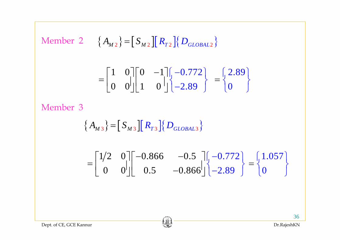
{ } [ ][ ]{ }R DA SM b 2 { } [ ][ ]{ }2 2 2 2T GLOBALM M R DA S=Member 2
0.7722
1 0 0 10 0 1 0 .89
−⎡ ⎤ ⎡ ⎤= ⎢ ⎥ ⎢ ⎥⎣ ⎦
−⎧ ⎫⎨
⎦ −⎩⎣⎬⎭
2.890⎧
=⎫
⎨ ⎬⎩ ⎭
Member 3
{ } [ ][ ]{ }3 3 3 3T GLOBALM M R DA S=
1 2 0 0.866 0.50 0 0.5 0.866
0.7722.89
− −⎡ ⎤ ⎡ ⎤= ⎢ ⎥ ⎢ ⎥−⎣ ⎦
−⎧ ⎫⎨
⎣ ⎦⎬−⎩ ⎭
1.0570
=⎧ ⎫⎨ ⎬⎩ ⎭⎣ ⎦ ⎣ ⎦ ⎩ ⎭ ⎩ ⎭
Dept. of CE, GCE Kannur Dr.RajeshKN
36
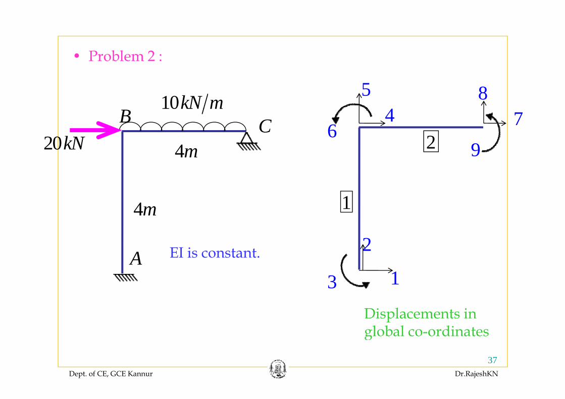
• Problem 2 :
10kN m5
48
4m
0kN mCB
20kN 24
6 794m
1
9
4m 1
2A EI is constant.
1
2
3Displacements in global co-ordinates
Dept. of CE, GCE Kannur Dr.RajeshKN
37
global co ordinates
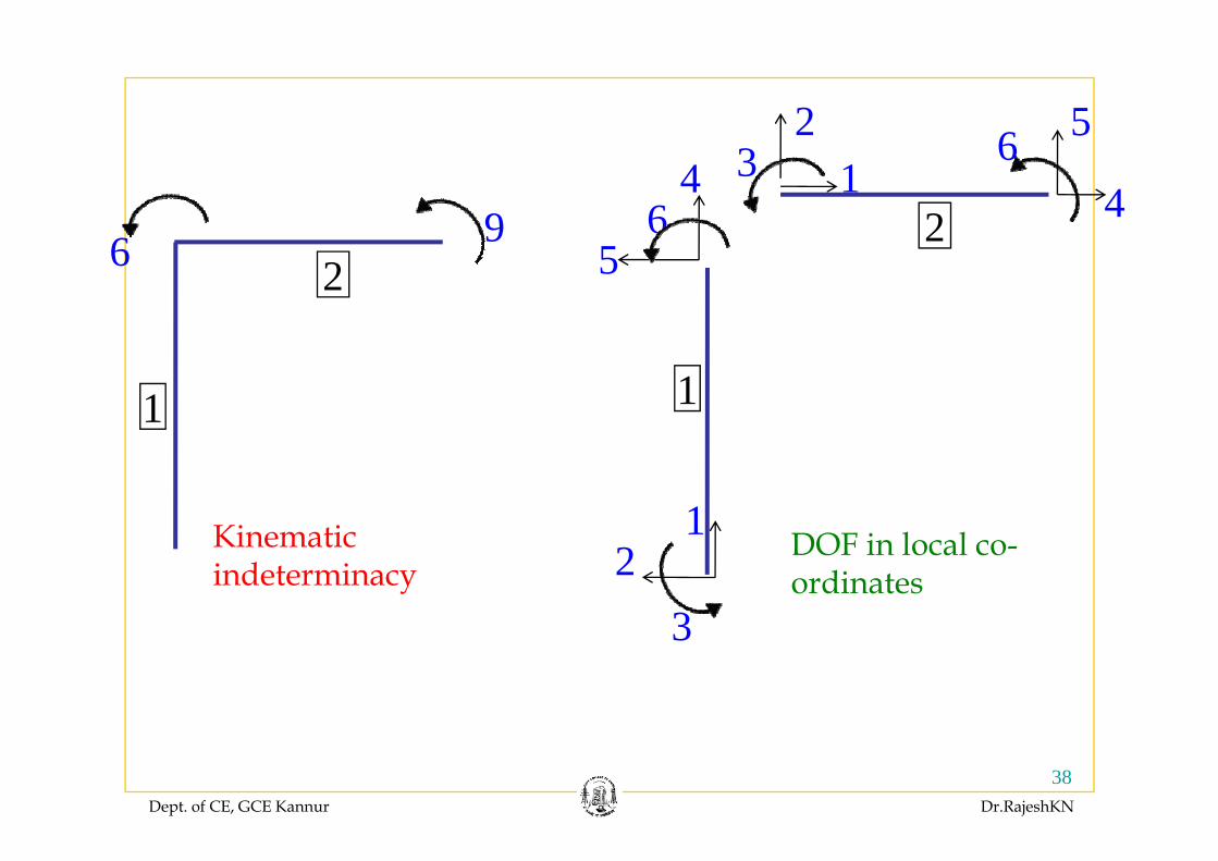
2 56
9 21 4
3 64
626 9 2
5
1 1
Ki ti 1Kinematic indeterminacy
DOF in local co-ordinates
12
33
Dept. of CE, GCE Kannur Dr.RajeshKN
38
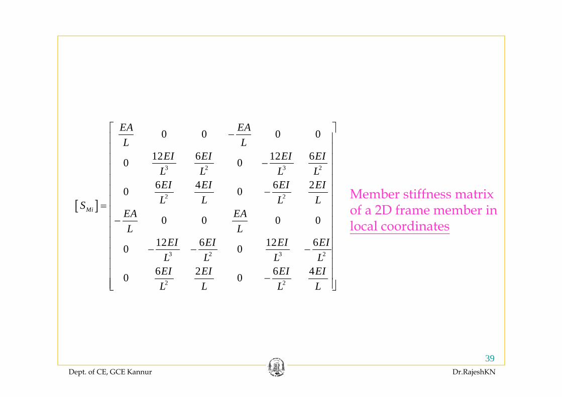
0 0 0 0
12 6 12 6
EA EAL L
EI EI EI EI
⎡ ⎤−⎢ ⎥⎢ ⎥⎢ ⎥
3 2 3 2
2 2
12 6 12 60 0
6 4 6 20 0
EI EI EI EIL L L LEI EI EI EIL L L L
⎢ ⎥⎢ ⎥−⎢ ⎥⎢ ⎥⎢ ⎥−⎢ ⎥
Member stiffness matrix [ ]
0 0 0 0
12 6 12 6
MiL L L LS
EA EAL L
EI EI EI EI
⎢ ⎥=⎢ ⎥−⎢ ⎥⎢ ⎥⎢ ⎥
of a 2D frame member in local coordinates
3 2 3 2
2 2
12 6 12 60 0
6 2 6 40 0
EI EI EI EIL L L LEI EI EI EIL L L L
⎢ ⎥− − −⎢ ⎥⎢ ⎥⎢ ⎥−⎢ ⎥⎣ ⎦L L L L⎢ ⎥⎣ ⎦
Dept. of CE, GCE Kannur Dr.RajeshKN
39
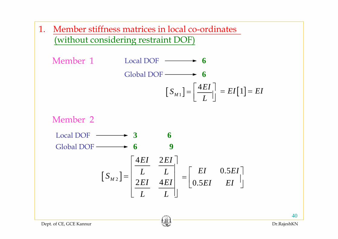
1. Member stiffness matrices in local co-ordinates ( ith t id i t i t DOF)
6Local DOFMember 1
(without considering restraint DOF)
[ ] 4EIS ⎡ ⎤= ⎢ ⎥ [ ]1EI EI= =
6Global DOF
[ ]1MSL
= ⎢ ⎥⎣ ⎦[ ]1EI EI
Member 2
6 9Global DOF3 6Local DOF
Member 2
[ ]4 2EI EI
L LS
⎡ ⎤⎢ ⎥⎢ ⎥
6 9Global DOF
0.5EI EI⎡ ⎤[ ]2 2 4ML LSEI EIL L
= ⎢ ⎥⎢ ⎥⎢ ⎥⎣ ⎦
0.5EI EI⎡ ⎤
= ⎢ ⎥⎣ ⎦
Dept. of CE, GCE Kannur Dr.RajeshKN
40
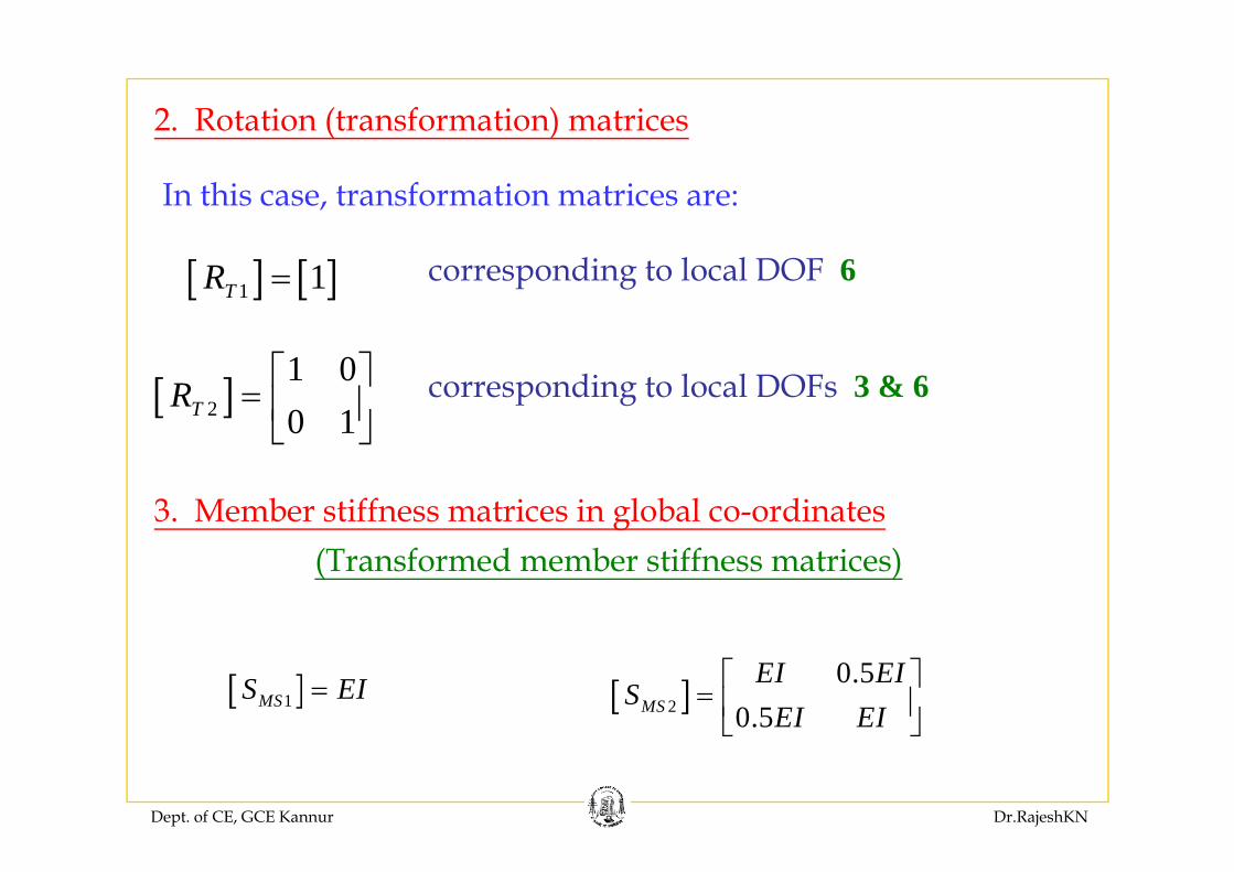
2. Rotation (transformation) matrices
In this case, transformation matrices are:
[ ] [ ]1 1TR = corresponding to local DOF 6
[ ]2
1 00 1TR ⎡ ⎤
= ⎢ ⎥⎣ ⎦
corresponding to local DOFs 3 & 6⎣ ⎦
3. Member stiffness matrices in global co-ordinates(Transformed member stiffness matrices)
[ ]1MSS EI= [ ]2
0.50.5MS
EI EIS
EI EI⎡ ⎤
= ⎢ ⎥⎣ ⎦
Dept. of CE, GCE Kannur Dr.RajeshKN
⎣ ⎦
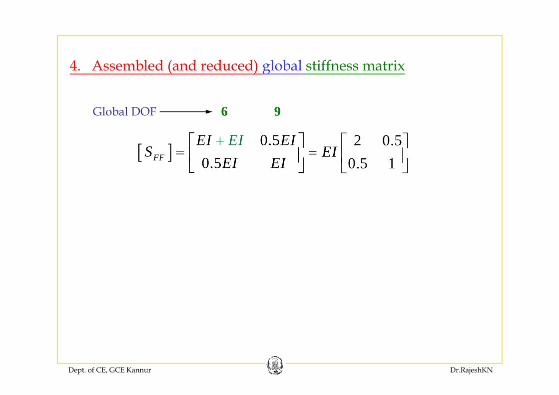
4 A bl d ( d d d) l b l tiff t i
6 9Gl b l DOF
4. Assembled (and reduced) global stiffness matrix
[ ] 0.5EI EIS
IE⎡ + ⎤= ⎢ ⎥
6 9Global DOF
2 0.5EI ⎡ ⎤
= ⎢ ⎥[ ]0.5FFS
EI EI= ⎢ ⎥⎣ ⎦ 0.5 1
EI= ⎢ ⎥⎣ ⎦
Dept. of CE, GCE Kannur Dr.RajeshKN
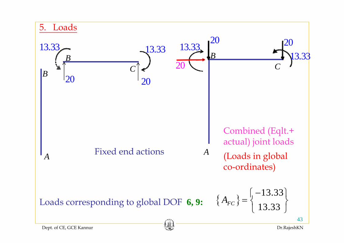
5. Loads20
13.33 13.33B
C
2013.33 20
13.33BC20
B 20 20C C20
Fi d d ti A
Combined (Eqlt.+ actual) joint loads
A Fixed end actions A (Loads in global co-ordinates)
{ }13.33
13 33FCA−⎧ ⎫
= ⎨ ⎬⎩ ⎭
Loads corresponding to global DOF 6, 9:
Dept. of CE, GCE Kannur Dr.RajeshKN
43
{ }13.33FC ⎨ ⎬
⎩ ⎭Loads corresponding to global DOF 6, 9:
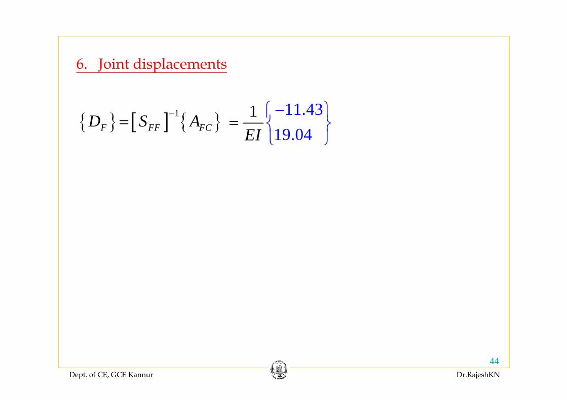
6 Joint displacements
11 431 ⎧ ⎫
6. Joint displacements
{ } [ ] { }1F FF FCD S A−=
11.4319.04
1EI
−⎧=
⎫⎨ ⎬⎩ ⎭
Dept. of CE, GCE Kannur Dr.RajeshKN
44
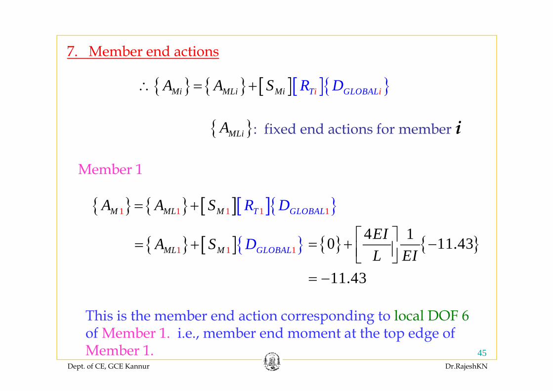
7. Member end actions
{ } { } [ ][ ]{ }Mi MLi Mi iT GLOB iALR DA A S∴ = +
: fixed end actions for member i{ }MLiA
Member 1
{ } { } [ ][ ]{ }1 1 1 1 1TM M G LM L BAL OR DA A S= +
{ } [ ]{ }DA S { } { }4 10 11 43EI⎡ ⎤{ } [ ]{ }1 1 1ML M GLOBALDA S= + { } { }0 11.43
11.43L EI
⎡ ⎤= + −⎢ ⎥⎣ ⎦= −
This is the member end action corresponding to local DOF 6 f M b 1 i b d h d f
Dept. of CE, GCE Kannur Dr.RajeshKN
45
of Member 1. i.e., member end moment at the top edge of Member 1.
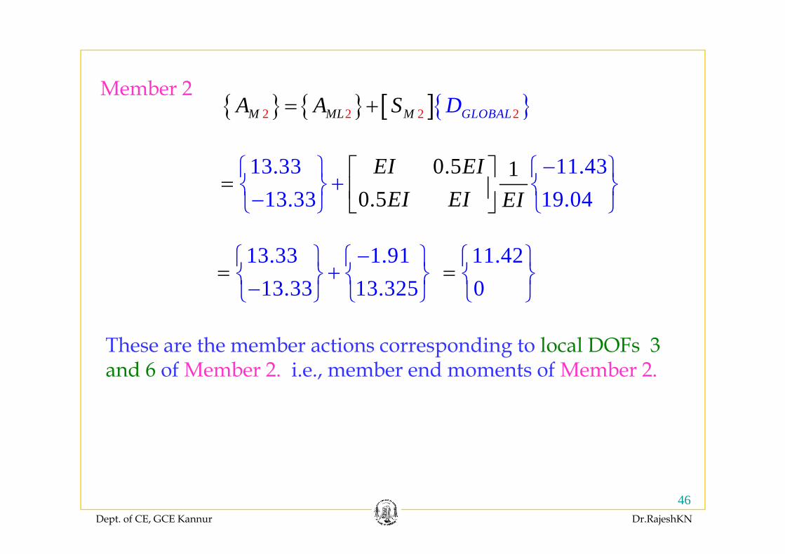
Member 2{ } { } [ ]{ }2 2 2 2M ML M GLOBALA A DS= +
Member 2
13.33 11.4313.33 1
0.59.04
10.5
EI EIEI EI EI
−⎧ ⎫ ⎧ ⎫+⎡ ⎤
= ⎢ ⎥⎣
⎨ ⎬ ⎨−⎩ ⎭ ⎩⎦⎬⎭
13.33 1.91−⎧ ⎫ ⎧ ⎫+⎨ ⎬ ⎨= ⎬
11.42=⎧ ⎫⎨ ⎬
Th th b ti di t l l DOF 3
13.33 13.325+⎨ ⎬ ⎨
⎩ ⎭⎬− ⎩ ⎭ 0⎨ ⎬
⎩ ⎭
These are the member actions corresponding to local DOFs 3 and 6 of Member 2. i.e., member end moments of Member 2.
Dept. of CE, GCE Kannur Dr.RajeshKN
46
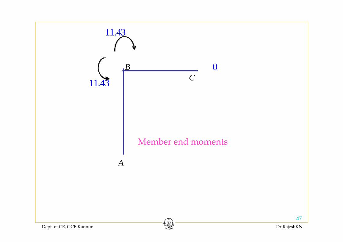
11.43
0B 0BC11.43
Member end moments
A
Dept. of CE, GCE Kannur Dr.RajeshKN
47
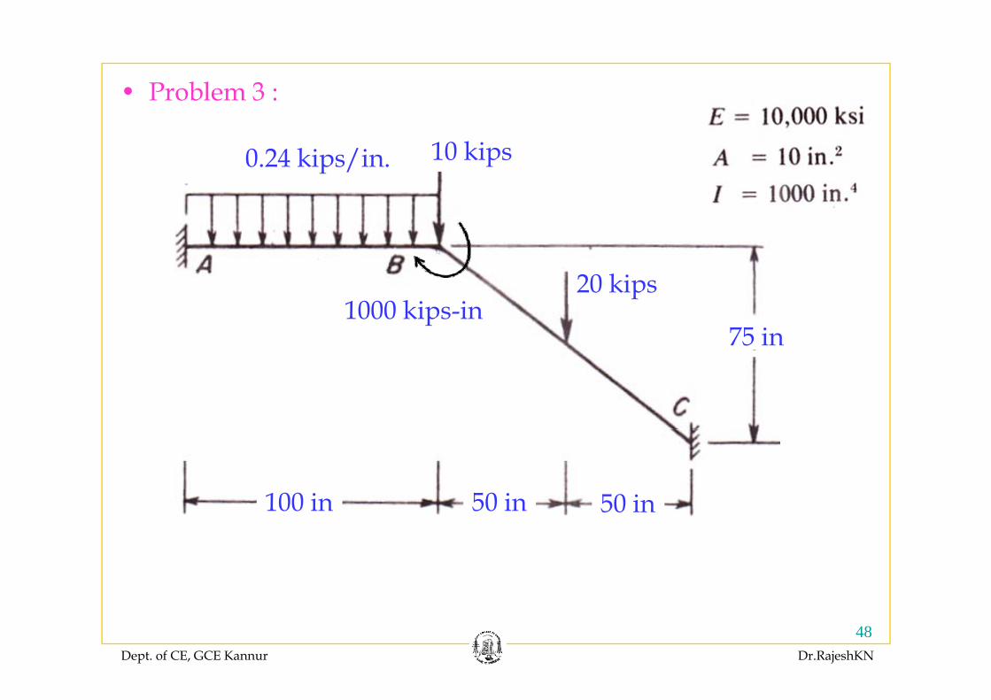
• Problem 3 :
10 kips0.24 kips/in.
20 kips1000 kips-in
75 in
100 in 50 in 50 in100 in 50 in 50 in
Dept. of CE, GCE Kannur Dr.RajeshKN
48
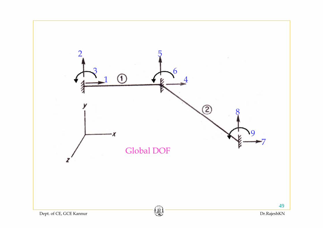
2 5
13
46
8
79
8
Global DOF7
Dept. of CE, GCE Kannur Dr.RajeshKN
49
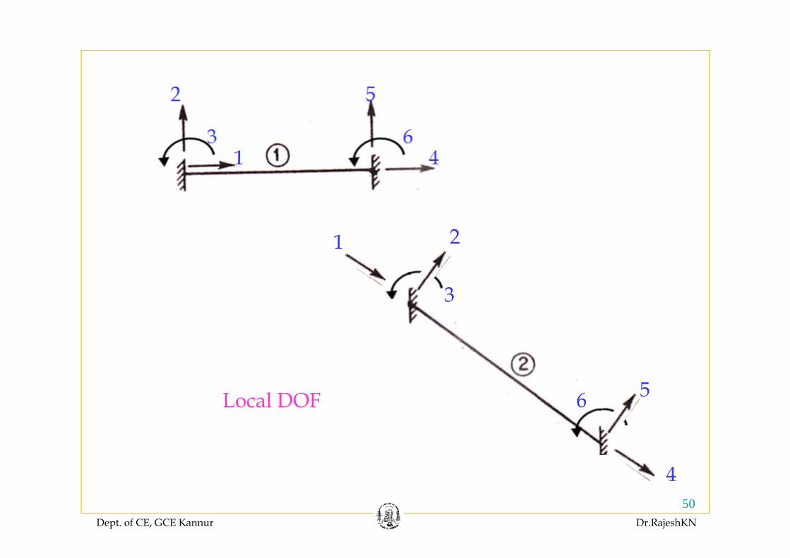
21
3
56Local DOF
4
6Local DOF
Dept. of CE, GCE Kannur Dr.RajeshKN
50
4
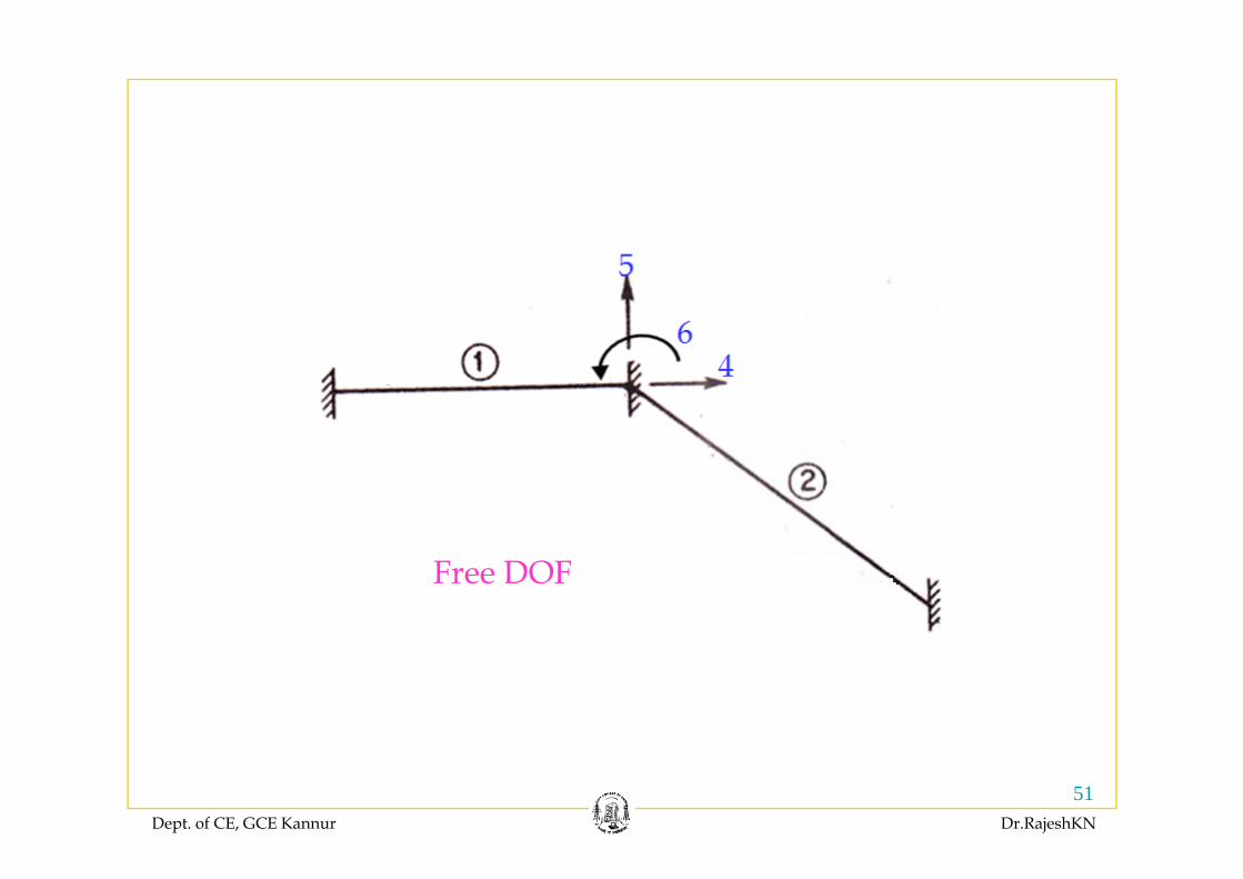
Free DOF
Dept. of CE, GCE Kannur Dr.RajeshKN
51
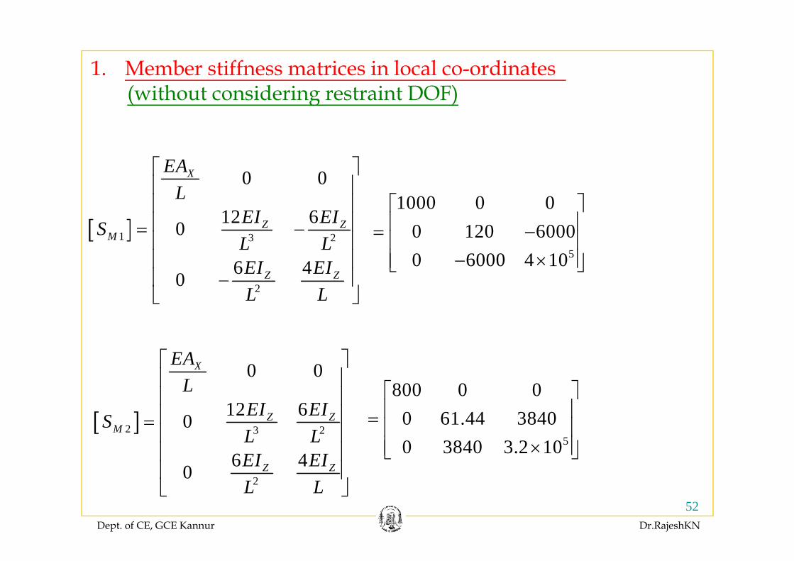
1. Member stiffness matrices in local co-ordinates ( ith t id i t i t DOF)(without considering restraint DOF)
0 0
12 6
XEAL
EI EI
⎡ ⎤⎢ ⎥⎢ ⎥⎢ ⎥
1000 0 0⎡ ⎤⎢ ⎥[ ]1 3 2
12 60
6 40
Z ZM
Z Z
EI EISL LEI EI
⎢ ⎥= −⎢ ⎥⎢ ⎥⎢ ⎥−
5
0 120 60000 6000 4 10
⎢ ⎥= −⎢ ⎥− ×⎢ ⎥⎣ ⎦
20L L
⎢ ⎥−⎣ ⎦
0 0
12 6
XEAL
EI EI
⎡ ⎤⎢ ⎥⎢ ⎥⎢ ⎥
800 0 0⎡ ⎤⎢ ⎥[ ]2 3 2
12 60
6 40
Z ZM
Z Z
EI EISL LEI EI
⎢ ⎥=⎢ ⎥⎢ ⎥⎢ ⎥
5
0 61.44 38400 3840 3.2 10
⎢ ⎥= ⎢ ⎥×⎢ ⎥⎣ ⎦
Dept. of CE, GCE Kannur Dr.RajeshKN
52
20L L
⎢ ⎥⎣ ⎦
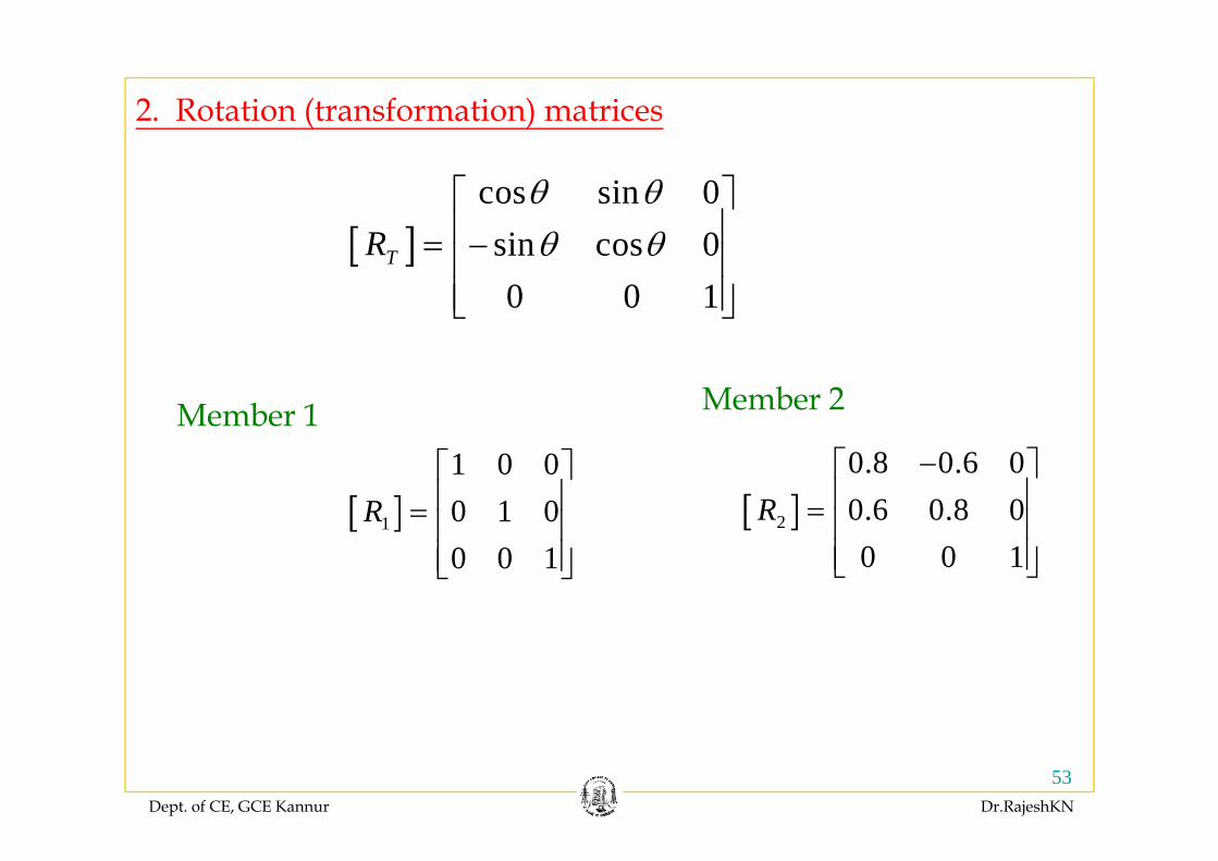
2. Rotation (transformation) matrices
[ ]cos sin 0
i 0R⎡ ⎤⎢ ⎥
θ θθ θ[ ] sin cos 0
0 0 1TR ⎢ ⎥= −⎢ ⎥
⎢ ⎥⎣ ⎦
θ θ
Member 1 Member 2
[ ]2
0.8 0.6 00.6 0.8 0R
−⎡ ⎤⎢ ⎥= ⎢ ⎥[ ]1
1 0 00 1 0R⎡ ⎤⎢ ⎥= ⎢ ⎥ [ ]
0 0 1⎢ ⎥⎢ ⎥⎣ ⎦
[ ]1
0 0 1⎢ ⎥⎢ ⎥⎣ ⎦
Dept. of CE, GCE Kannur Dr.RajeshKN
53

3. Member stiffness matrices in global co-ordinates(Transformed member stiffness matrices)
[ ] [ ] [ ][ ]1 1 1 1T
MS T M TS R S R=
1 0 0 1000 0 0 1 0 00 1 0 0 120 6000 0 1 0
T⎡ ⎤ ⎡ ⎤ ⎡ ⎤⎢ ⎥ ⎢ ⎥ ⎢ ⎥= ⎢ ⎥ ⎢ ⎥ ⎢ ⎥
5
0 1 0 0 120 6000 0 1 00 0 1 0 6000 4 10 0 0 1
= −⎢ ⎥ ⎢ ⎥ ⎢ ⎥− ×⎢ ⎥ ⎢ ⎥ ⎢ ⎥⎣ ⎦ ⎣ ⎦ ⎣ ⎦
5
1000 0 00 120 6000
⎡ ⎤⎢ ⎥= −⎢ ⎥⎢ ⎥50 6000 4 10− ×⎢ ⎥⎣ ⎦
Dept. of CE, GCE Kannur Dr.RajeshKN
54
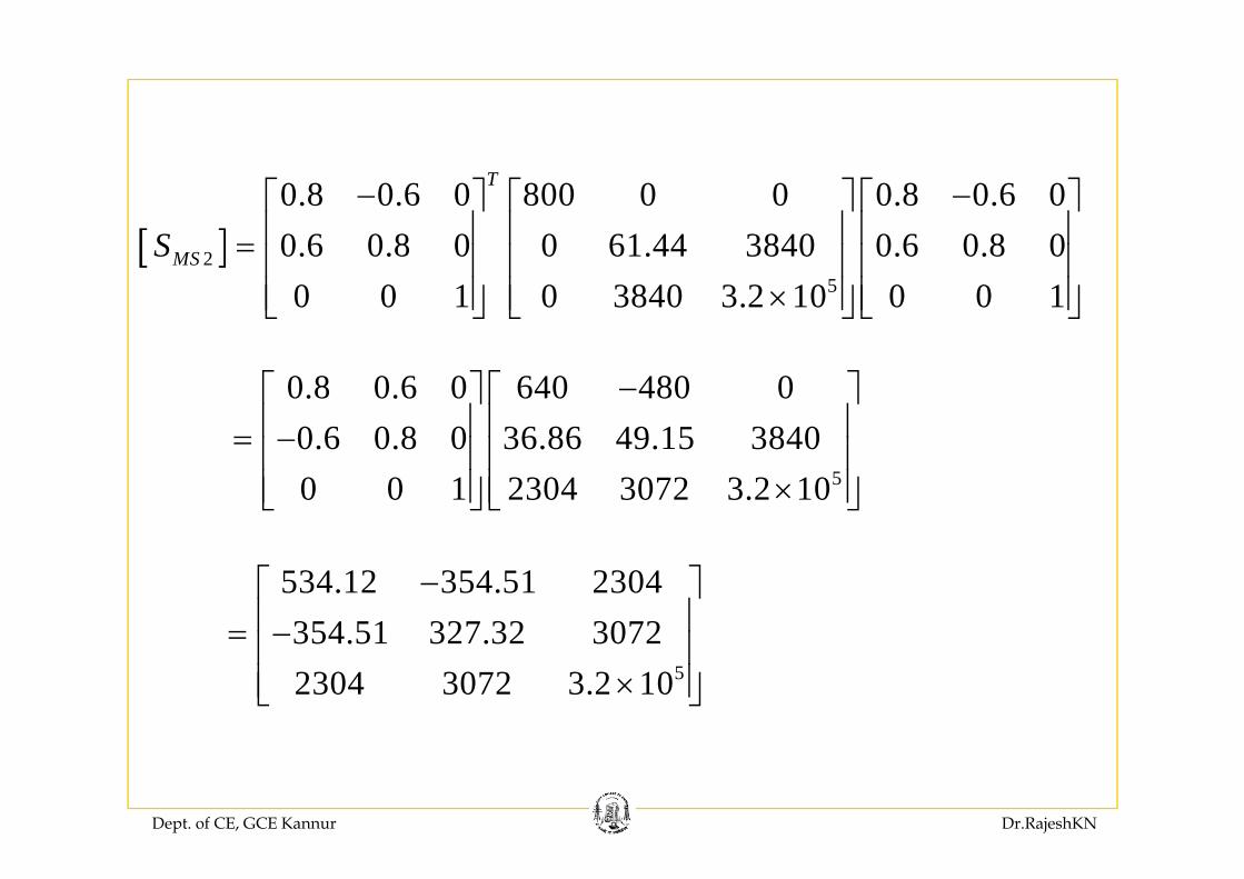
[ ]0.8 0.6 0 800 0 0 0.8 0.6 00 6 0 8 0 0 61 44 3840 0 6 0 8 0
T
S− −⎡ ⎤ ⎡ ⎤ ⎡ ⎤
⎢ ⎥ ⎢ ⎥ ⎢ ⎥[ ]25
0.6 0.8 0 0 61.44 3840 0.6 0.8 00 0 1 0 3840 3.2 10 0 0 1
MSS ⎢ ⎥ ⎢ ⎥ ⎢ ⎥= ⎢ ⎥ ⎢ ⎥ ⎢ ⎥×⎢ ⎥ ⎢ ⎥ ⎢ ⎥⎣ ⎦ ⎣ ⎦ ⎣ ⎦
0.8 0.6 0 640 480 00 6 0 8 0 36 86 49 15 3840
−⎡ ⎤ ⎡ ⎤⎢ ⎥ ⎢ ⎥= −⎢ ⎥ ⎢ ⎥
5
0.6 0.8 0 36.86 49.15 38400 0 1 2304 3072 3.2 10
= −⎢ ⎥ ⎢ ⎥×⎢ ⎥ ⎢ ⎥⎣ ⎦ ⎣ ⎦
534.12 354.51 2304354 51 327 32 3072
−⎡ ⎤⎢ ⎥= −⎢ ⎥
5
354.51 327.32 30722304 3072 3.2 10
⎢ ⎥×⎢ ⎥⎣ ⎦
Dept. of CE, GCE Kannur Dr.RajeshKN
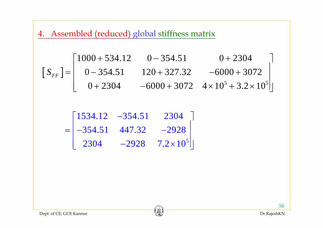
4. Assembled (reduced) global stiffness matrix
1000 534.12 0 354.51 0 2304+ − +⎡ ⎤
. sse b ed ( educed) g oba st ess at x
[ ]5 5
0 354.51 120 327.32 6000 30720 2304 6000 3072 4 10 3.2 10
FFS⎡ ⎤⎢ ⎥= − + − +⎢ ⎥
+ − + × + ×⎢ ⎥⎣ ⎦0 2304 6000 3072 4 10 3.2 10+ + × + ×⎢ ⎥⎣ ⎦
1534 12 354 51 2304⎡ ⎤
5
1534.12 354.51 2304354.51 447.32 2928
−⎡ ⎤⎢ ⎥− −⎢⎢
= ⎥⎥52304 2928 7.2 10− ×⎢⎣ ⎦⎥
Dept. of CE, GCE Kannur Dr.RajeshKN
56
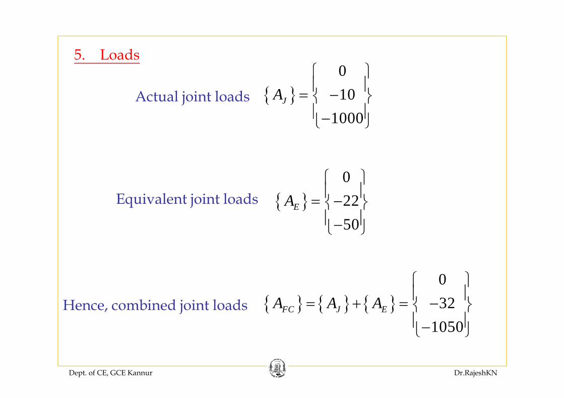
5. Loads⎧ ⎫
{ }010JA
⎧ ⎫⎪ ⎪= −⎨ ⎬⎪ ⎪
Actual joint loads1000⎪ ⎪−⎩ ⎭
{ }022A
⎧ ⎫⎪ ⎪⎨ ⎬Equivalent joint loads { } 22
50EA = −⎨ ⎬
⎪ ⎪−⎩ ⎭
Equivalent joint loads
0⎧ ⎫⎪ ⎪{ } { } { } 32
1050FC J EA A A ⎪ ⎪= + = −⎨ ⎬
⎪ ⎪−⎩ ⎭
Hence, combined joint loads
Dept. of CE, GCE Kannur Dr.RajeshKN
⎩ ⎭
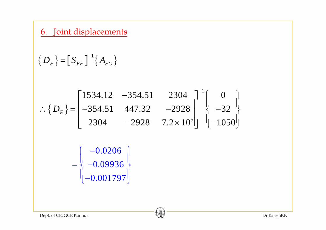
6. Joint displacements
{ } [ ] { }1F FF FCD S A−={ } [ ] { }F FF FCD S A
1
{ }
11534.12 354.51 2304 0354.51 447.32 2928 32FD
−− ⎧ ⎫⎡ ⎤⎪ ⎪⎢ ⎥∴ = − − −⎨ ⎬⎢ ⎥ ⎪ ⎪52304 2928 7.2 10 1050
⎢ ⎥ ⎪ ⎪− × −⎢ ⎥ ⎩ ⎭⎣ ⎦
0.02060.09936−⎧ ⎫
⎪ ⎪= −⎨ ⎬0.099360.001797
⎨ ⎬⎪ ⎪−⎩ ⎭
Dept. of CE, GCE Kannur Dr.RajeshKN
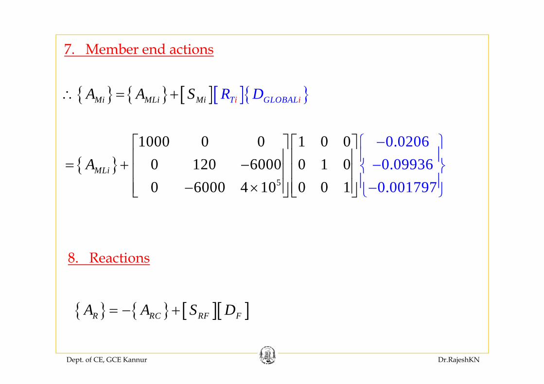
7. Member end actions
{ } { } [ ][ ]{ }Mi MLi Mi iT GLOB iALR DA A S∴ = +
1000 0 0 1 0 0 0.0206⎡ ⎤ ⎡ ⎤ −⎧ ⎫⎪ ⎪{ }
5
0 120 6000 0 1 0 0.09930 6000 4 10 0
60 1 0.001797
MLiA⎡ ⎤ ⎡ ⎤⎢ ⎥ ⎢ ⎥= + −⎢ ⎥ ⎢ ⎥
− ×⎢ ⎥ ⎢ ⎥
⎧ ⎫⎪ ⎪−⎨
⎣ ⎦ ⎣⎪⎩⎦
⎬⎪− ⎭0 6000 4 10 0 0 1 0.001797⎢ ⎥ ⎢ ⎥⎣ ⎦ ⎣ ⎩⎦ ⎭
8. Reactions
{ } { } [ ][ ]R RC RF FA A S D= − +
Dept. of CE, GCE Kannur Dr.RajeshKN
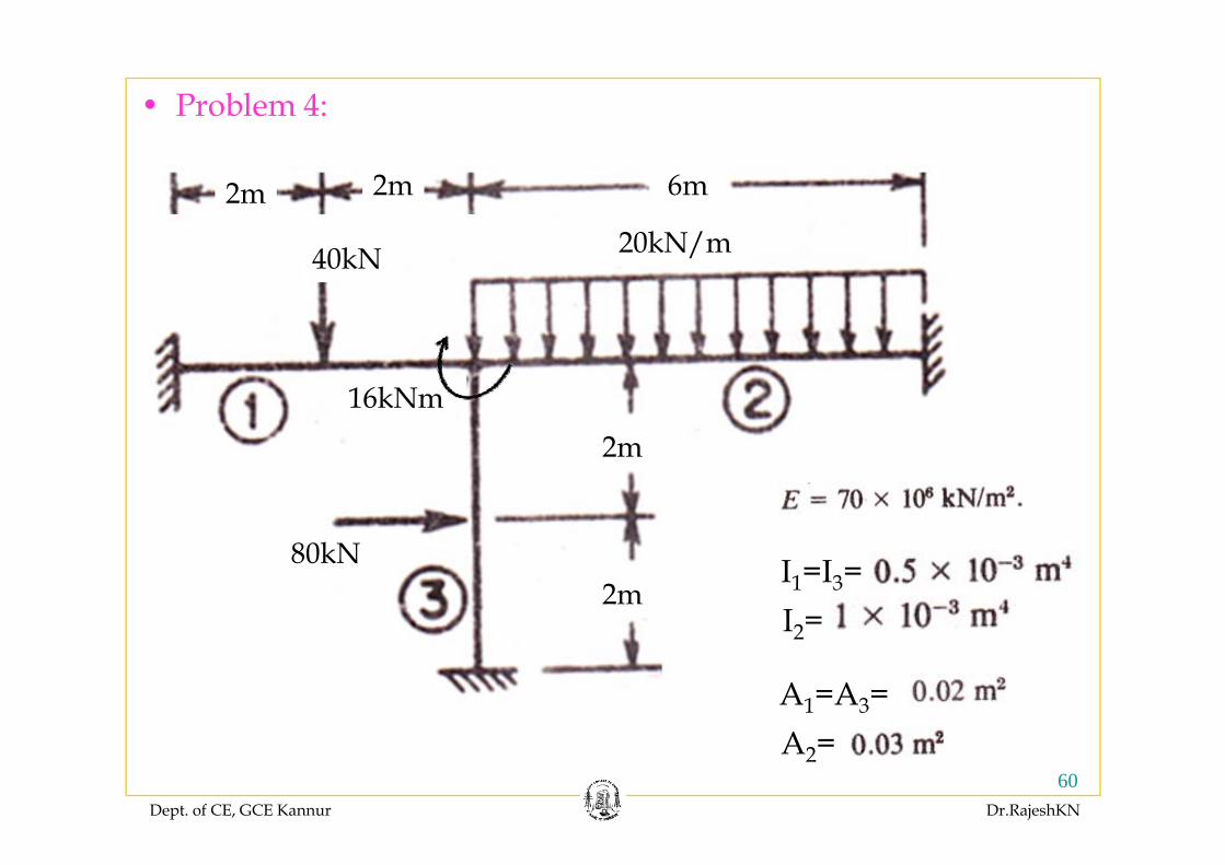
• Problem 4:
20kN/
6m2m2m
40kN 20kN/m
16kNm
2m
80kN2m
I1=I3=I2=I2
A1=A3=
Dept. of CE, GCE Kannur Dr.RajeshKN
60
A2=
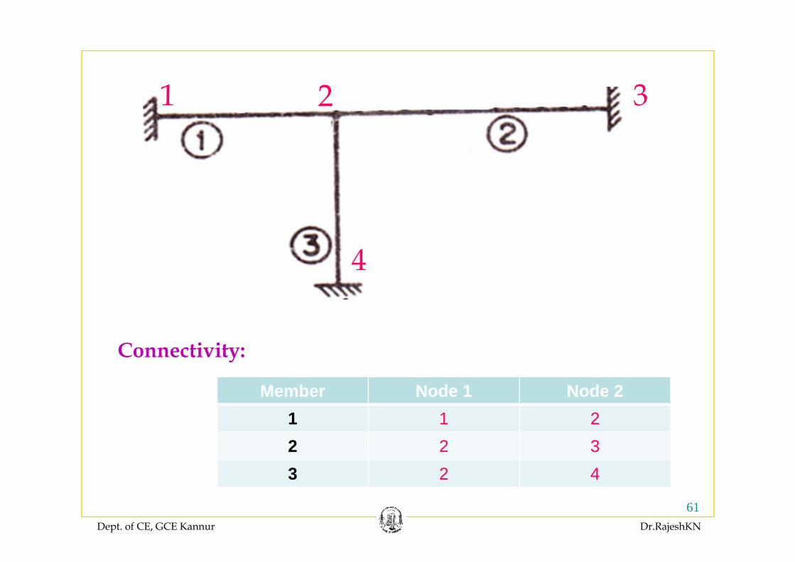
1 2 31 2 3
4
C ti itConnectivity:
Member Node 1 Node 21 1 22 2 33 2 4
Dept. of CE, GCE Kannur Dr.RajeshKN
61
3 2 4
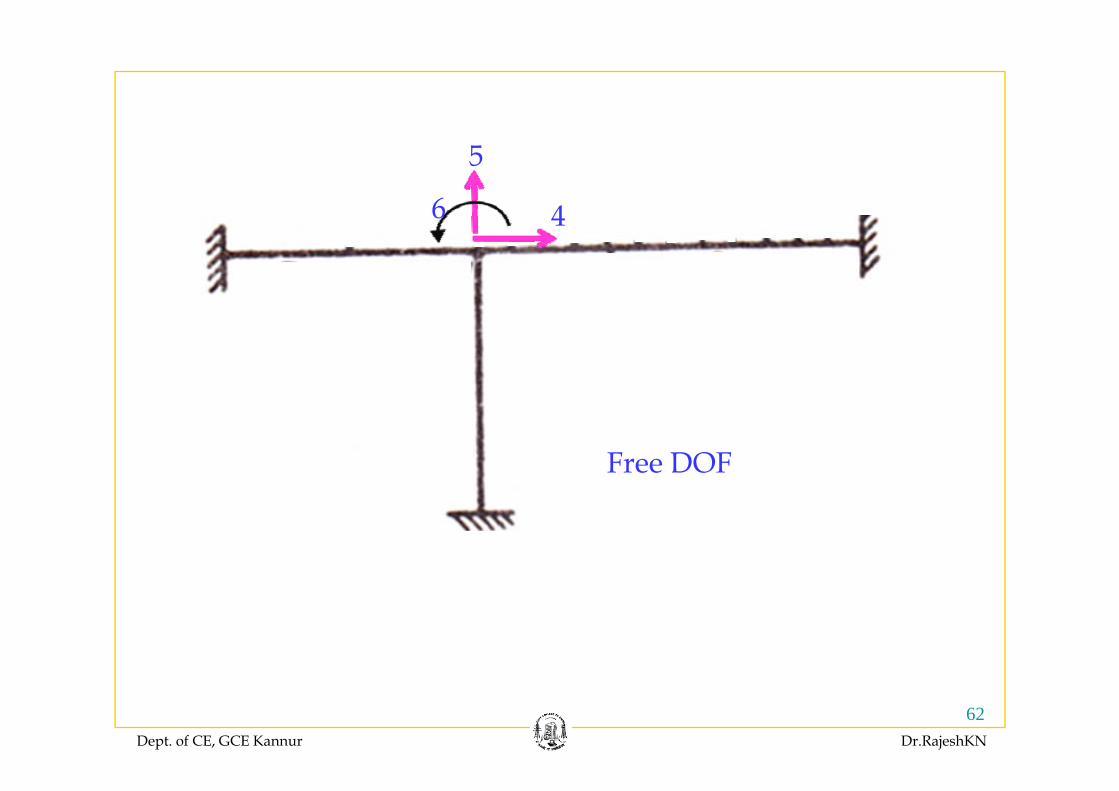
46
5
46
Free DOF
Dept. of CE, GCE Kannur Dr.RajeshKN
62
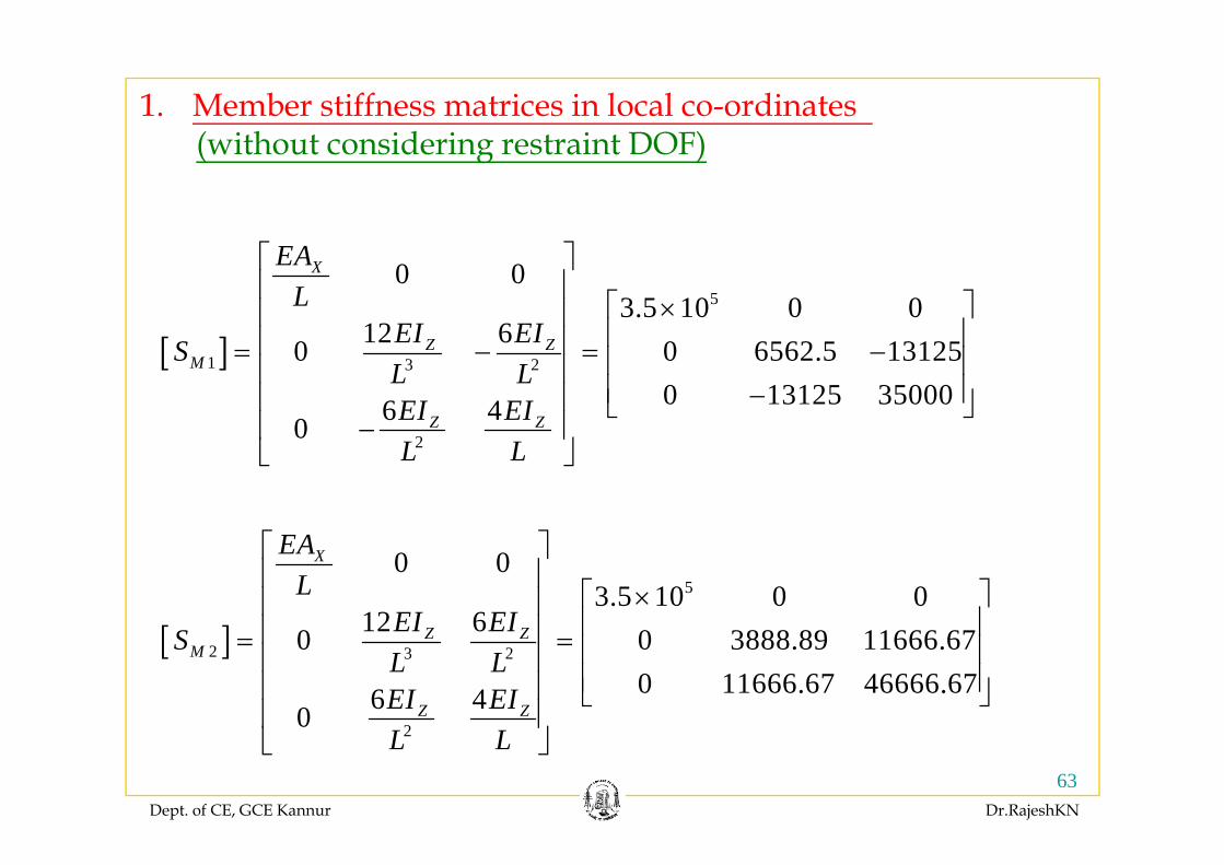
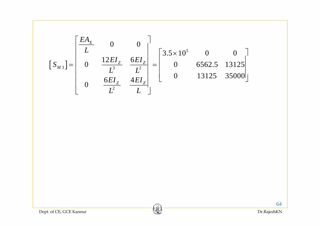
1. Member stiffness matrices in local co-ordinates ( ith t id i t i t DOF)(without considering restraint DOF)
50 0
3.5 10 0 012 6
XEAL
EI EI
⎡ ⎤⎢ ⎥
⎡ ⎤×⎢ ⎥⎢ ⎥⎢ ⎥[ ]1 3 2
12 60 0 6562.5 131250 13125 350006 40
Z ZM
Z Z
EI EISL LEI EI
⎢ ⎥⎢ ⎥= − = −⎢ ⎥⎢ ⎥⎢ ⎥−⎢ ⎥ ⎣ ⎦
⎢ ⎥− 20L L
⎢ ⎥⎣ ⎦
⎡ ⎤
[ ]5
0 03.5 10 0 0
12 6
X
Z Z
EAL
EI EI
⎡ ⎤⎢ ⎥
⎡ ⎤×⎢ ⎥⎢ ⎥⎢ ⎥[ ]2 3 2
2
12 60 0 3888.89 11666.670 11666.67 46666.676 40
Z ZM
Z Z
EI EISL LEI EI
⎢ ⎥⎢ ⎥= = ⎢ ⎥⎢ ⎥⎢ ⎥⎢ ⎥ ⎣ ⎦
⎢ ⎥⎣ ⎦
Dept. of CE, GCE Kannur Dr.RajeshKN
63
2L L⎢ ⎥⎣ ⎦
⎡ ⎤
[ ]5
0 03.5 10 0 0
12 60 0 6 62 1312
X
Z Z
EAL
EI EIS
⎡ ⎤⎢ ⎥
⎡ ⎤×⎢ ⎥⎢ ⎥⎢ ⎥[ ]3 3 2
2
12 60 0 6562.5 131250 13125 350006 40
Z ZM
Z Z
EI EISL LEI EI
⎢ ⎥⎢ ⎥= = ⎢ ⎥⎢ ⎥⎢ ⎥⎢ ⎥ ⎣ ⎦
⎢ ⎥⎣ ⎦2L L⎢ ⎥⎣ ⎦
Dept. of CE, GCE Kannur Dr.RajeshKN
64
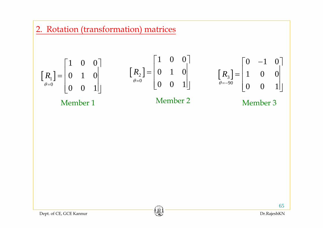
2. Rotation (transformation) matrices
0 1 0−⎡ ⎤1 0 0⎡ ⎤ 1 0 0⎡ ⎤
[ ]390
0 1 01 0 00 0 1
Rθ =−
⎡ ⎤⎢ ⎥= ⎢ ⎥⎢ ⎥⎣ ⎦
[ ]10
1 0 00 1 00 0 1
Rθ =
⎡ ⎤⎢ ⎥= ⎢ ⎥⎢ ⎥⎣ ⎦
[ ]20
0 1 00 0 1
Rθ =
⎡ ⎤⎢ ⎥= ⎢ ⎥⎢ ⎥⎣ ⎦
Member 1
0 0 1⎢ ⎥⎣ ⎦Member 2
0 0 1⎢ ⎥⎣ ⎦Member 3
⎣ ⎦
Dept. of CE, GCE Kannur Dr.RajeshKN
65
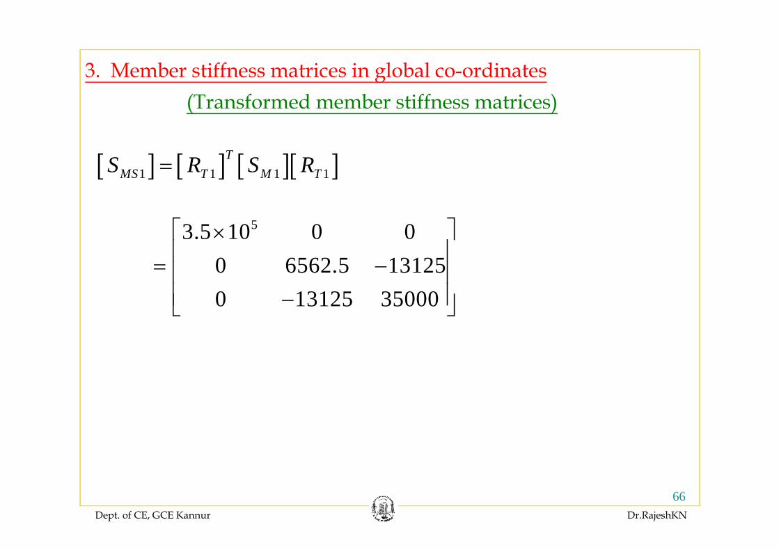
3. Member stiffness matrices in global co-ordinates(Transformed member stiffness matrices)
[ ] [ ] [ ][ ]1 1 1 1T
MS T M TS R S R=
53.5 10 0 00 6562.5 13125
⎡ ⎤×⎢ ⎥= −⎢ ⎥
0 13125 35000⎢ ⎥⎢ ⎥−⎣ ⎦
Dept. of CE, GCE Kannur Dr.RajeshKN
66
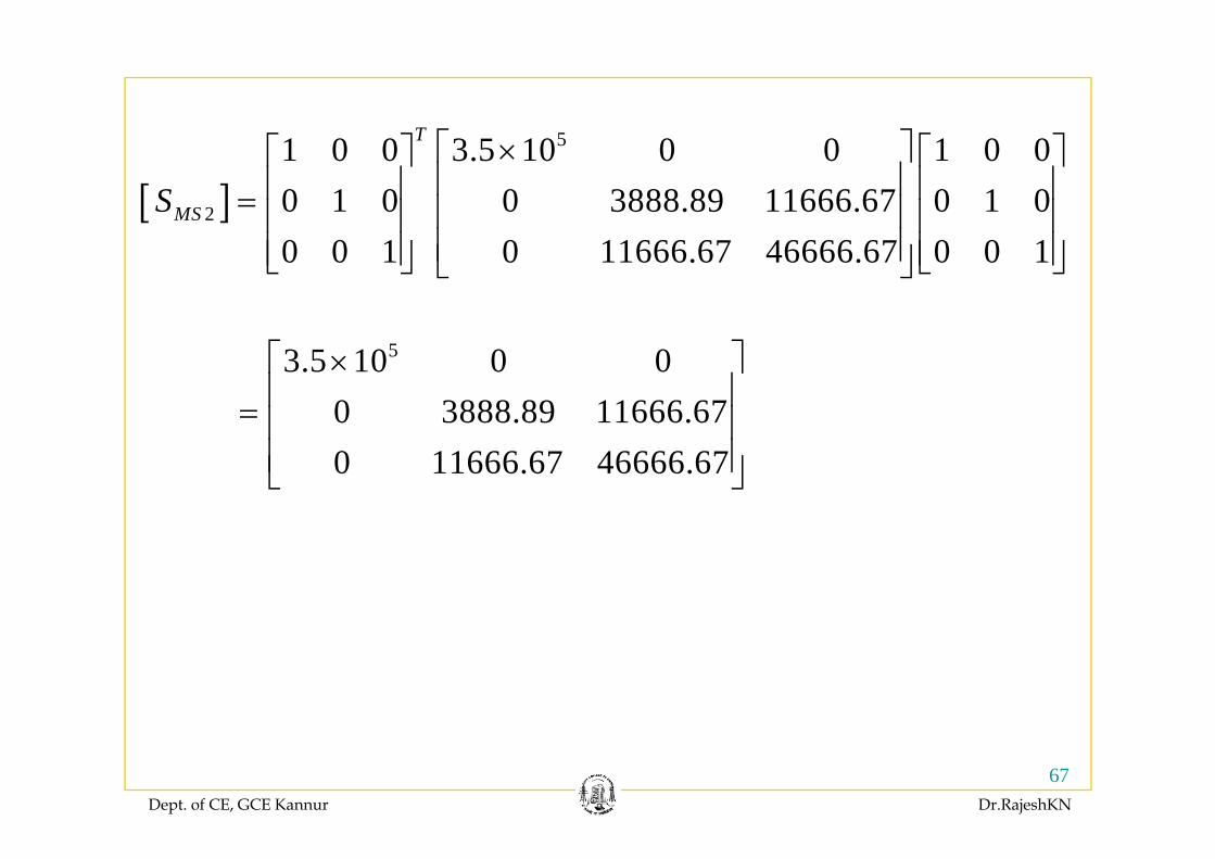
5T ⎡ ⎤⎡ ⎤ ⎡ ⎤[ ]
5
2
1 0 0 3.5 10 0 0 1 0 00 1 0 0 3888.89 11666.67 0 1 0
T
MSS⎡ ⎤×⎡ ⎤ ⎡ ⎤⎢ ⎥⎢ ⎥ ⎢ ⎥= ⎢ ⎥⎢ ⎥ ⎢ ⎥⎢ ⎥⎢ ⎥ ⎢ ⎥0 0 1 0 11666.67 46666.67 0 0 1⎢ ⎥⎢ ⎥ ⎢ ⎥⎣ ⎦ ⎣ ⎦⎣ ⎦
53.5 10 0 00 3888.89 11666.67
⎡ ⎤×⎢ ⎥= ⎢ ⎥
0 11666.67 46666.67⎢ ⎥⎢ ⎥⎣ ⎦
Dept. of CE, GCE Kannur Dr.RajeshKN
67
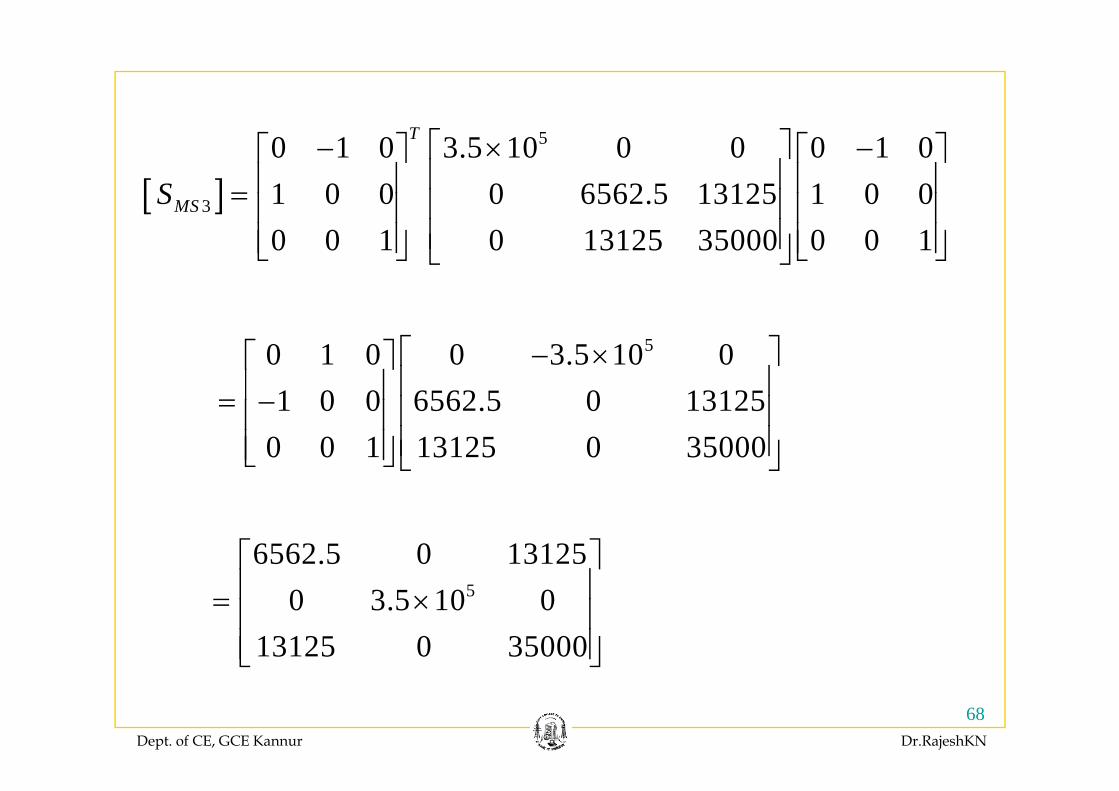
[ ]5
3
0 1 0 3.5 10 0 0 0 1 01 0 0 0 6562.5 13125 1 0 0
T
MSS⎡ ⎤− × −⎡ ⎤ ⎡ ⎤⎢ ⎥⎢ ⎥ ⎢ ⎥= ⎢ ⎥⎢ ⎥ ⎢ ⎥
0 0 1 0 13125 35000 0 0 1⎢ ⎥⎢ ⎥ ⎢ ⎥⎢ ⎥⎢ ⎥ ⎢ ⎥⎣ ⎦ ⎣ ⎦⎣ ⎦
50 1 0 0 3.5 10 01 0 0 6562 5 0 13125
⎡ ⎤− ×⎡ ⎤⎢ ⎥⎢ ⎥⎢ ⎥1 0 0 6562.5 0 13125
0 0 1 13125 0 35000
⎢ ⎥⎢ ⎥= − ⎢ ⎥⎢ ⎥⎢ ⎥⎢ ⎥⎣ ⎦ ⎣ ⎦
6562.5 0 13125⎡ ⎤⎢ ⎥50 3.5 10 0
13125 0 35000
⎢ ⎥= ×⎢ ⎥⎢ ⎥⎣ ⎦
Dept. of CE, GCE Kannur Dr.RajeshKN
68
⎣ ⎦
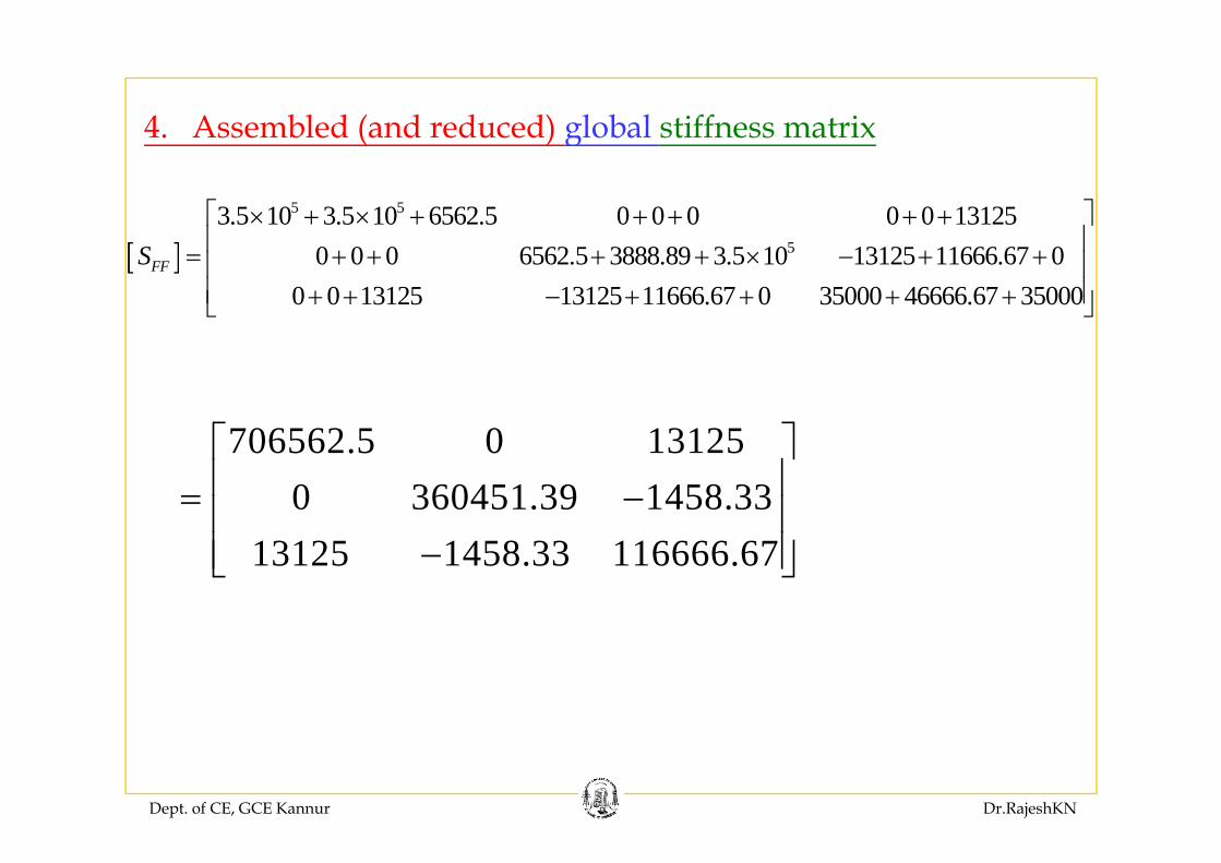
4. Assembled (and reduced) global stiffness matrix. sse b ed (a d educed) g oba st ess at x
5 53.5 10 3.5 10 6562.5 0 0 0 0 0 13125⎡ ⎤× + × + + + + +⎢ ⎥[ ] 50 0 0 6562.5 3888.89 3.5 10 13125 11666.67 0
0 0 13125 13125 11666.67 0 35000 46666.67 35000FFS ⎢ ⎥= + + + + × − + +⎢ ⎥
⎢ ⎥+ + − + + + +⎣ ⎦
706562 5 0 13125⎡ ⎤706562.5 0 131250 360451.39 1458.33
⎡ ⎤⎢ ⎥= −⎢ ⎥
13125 1458.33 116666.67⎢ ⎥
−⎢ ⎥⎣ ⎦
Dept. of CE, GCE Kannur Dr.RajeshKN
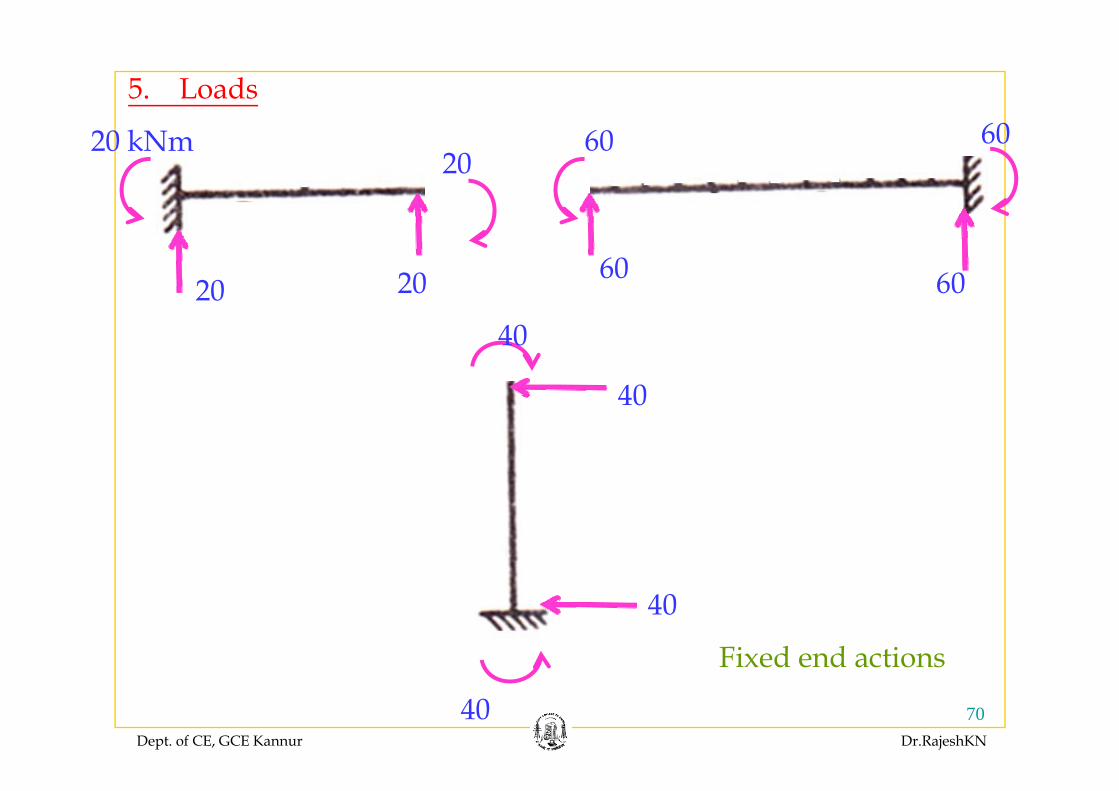
605. Loads
2020 kNm 60 60
202060 60
40
4040
40
Fixed end actions
Dept. of CE, GCE Kannur Dr.RajeshKN
7040
Fixed end actions
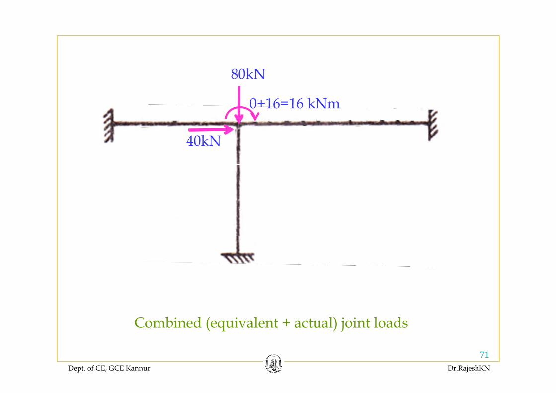
80kN
0+16=16 kNm0 16 16 kNm
40kN
Combined (equivalent + actual) joint loads
Dept. of CE, GCE Kannur Dr.RajeshKN
71
( q ) j
0⎧ ⎫ 0⎧ ⎫ 0⎧ ⎫0⎧ ⎫
⎪ ⎪000
⎧ ⎫⎪ ⎪⎪ ⎪⎪ ⎪
02020
⎧ ⎫⎪ ⎪−⎪ ⎪−⎪ ⎪
02020
⎧ ⎫⎪ ⎪−⎪ ⎪−⎪ ⎪
20200
⎪ ⎪−⎪ ⎪−⎪ ⎪
⎪ ⎪00
⎪ ⎪⎪ ⎪⎪ ⎪⎪ ⎪⎪ ⎪
4080
⎪ ⎪⎪ ⎪⎪ ⎪⎪ ⎪−⎪ ⎪
4080
⎪ ⎪⎪ ⎪⎪ ⎪⎪ ⎪−⎪ ⎪
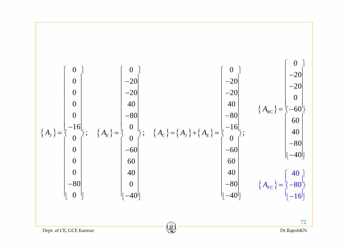
{ }060
60RCA
⎪ ⎪⎪ ⎪⎪ ⎪= −⎨ ⎬⎪ ⎪⎪ ⎪
{ }16
;00
JA⎪ ⎪−⎪ ⎪= ⎨ ⎬⎪ ⎪⎪ ⎪
{ }0
;060
EA⎪ ⎪⎪ ⎪= ⎨ ⎬⎪ ⎪⎪ ⎪−
{ } { } { }16
;060
C J EA A A⎪ ⎪−⎪ ⎪= + = ⎨ ⎬⎪ ⎪⎪ ⎪−
4080
⎪ ⎪⎪ ⎪⎪ ⎪−⎪ ⎪⎪ ⎪
000
⎪ ⎪⎪ ⎪⎪ ⎪⎪ ⎪⎪ ⎪
606040
⎪ ⎪⎪ ⎪⎪ ⎪⎪ ⎪⎪ ⎪
40⎧ ⎫⎪ ⎪
606040
⎪ ⎪⎪ ⎪⎪ ⎪⎪ ⎪⎪ ⎪
40⎪ ⎪−⎩ ⎭
800
⎪ ⎪−⎪ ⎪
⎪ ⎪⎩ ⎭
040
⎪ ⎪⎪ ⎪⎪ ⎪−⎩ ⎭
{ } 8016
FCA ⎪ ⎪= −⎨ ⎬⎪ ⎪−⎩ ⎭
8040
⎪ ⎪−⎪ ⎪
⎪ ⎪−⎩ ⎭
Dept. of CE, GCE Kannur Dr.RajeshKN
72
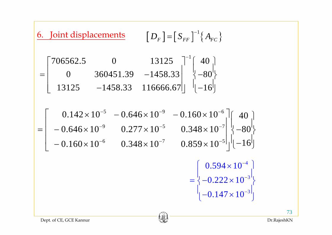
[ ] [ ] { }1D S A−=6. Joint displacements
1706562.5 0 13125 40−⎡ ⎤ ⎧ ⎫
⎪ ⎪
[ ] [ ] { }F FF FCD S A=6. Jo t d sp ace e ts
0 360451.39 1458.33 8013125 1458.33 116666.67 16
⎡ ⎤ ⎧ ⎫⎪ ⎪⎢ ⎥= − −⎨ ⎬⎢ ⎥ ⎪ ⎪− −⎢ ⎥⎣ ⎦ ⎩ ⎭⎢ ⎥⎣ ⎦ ⎩ ⎭
5 9 60.142 10 0.646 10 0.160 10 40 − − −⎡ ⎤× − × − × ⎧ ⎫⎢ ⎥9 5 7
6 7 5
400.646 10 0.277 10 0.348 10 80
160 160 10 0 348 10 0 859 10 − − −
− − −
⎡ ⎤ ⎧ ⎫⎢ ⎥ ⎪ ⎪= − × × × −⎨ ⎬⎢ ⎥
⎪ ⎪⎢ ⎥ −× × × ⎩ ⎭⎣ ⎦ 160.160 10 0.348 10 0.859 10 ⎢ ⎥− × × × ⎩ ⎭⎣ ⎦
40.594 10 −⎧ ⎫×⎪ ⎪3
3
0.222 100.147 10
−
−
⎪ ⎪= − ×⎨ ⎬⎪ ⎪− ×⎩ ⎭
Dept. of CE, GCE Kannur Dr.RajeshKN
73
⎩ ⎭
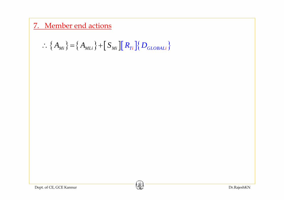
7. Member end actions
{ } { } [ ][ ]{ }Mi MLi Mi iT GLOB iALR DA A S∴ = +
Dept. of CE, GCE Kannur Dr.RajeshKN
Summary
Direct stiffness method
Summary
• Introduction – element stiffness matrix – rotation transformation matrix – transformation of displacement and load vectors and stiffness matrix – equivalent nodal forces and load vectors –assembly of stiffness matrix and load vector – determination of assembly of stiffness matrix and load vector determination of nodal displacement and element forces – analysis of plane truss beam and plane frame (with numerical examples) – analysis of grid space frame (without numerical examples) grid – space frame (without numerical examples)
Dept. of CE, GCE Kannur Dr.RajeshKN
75
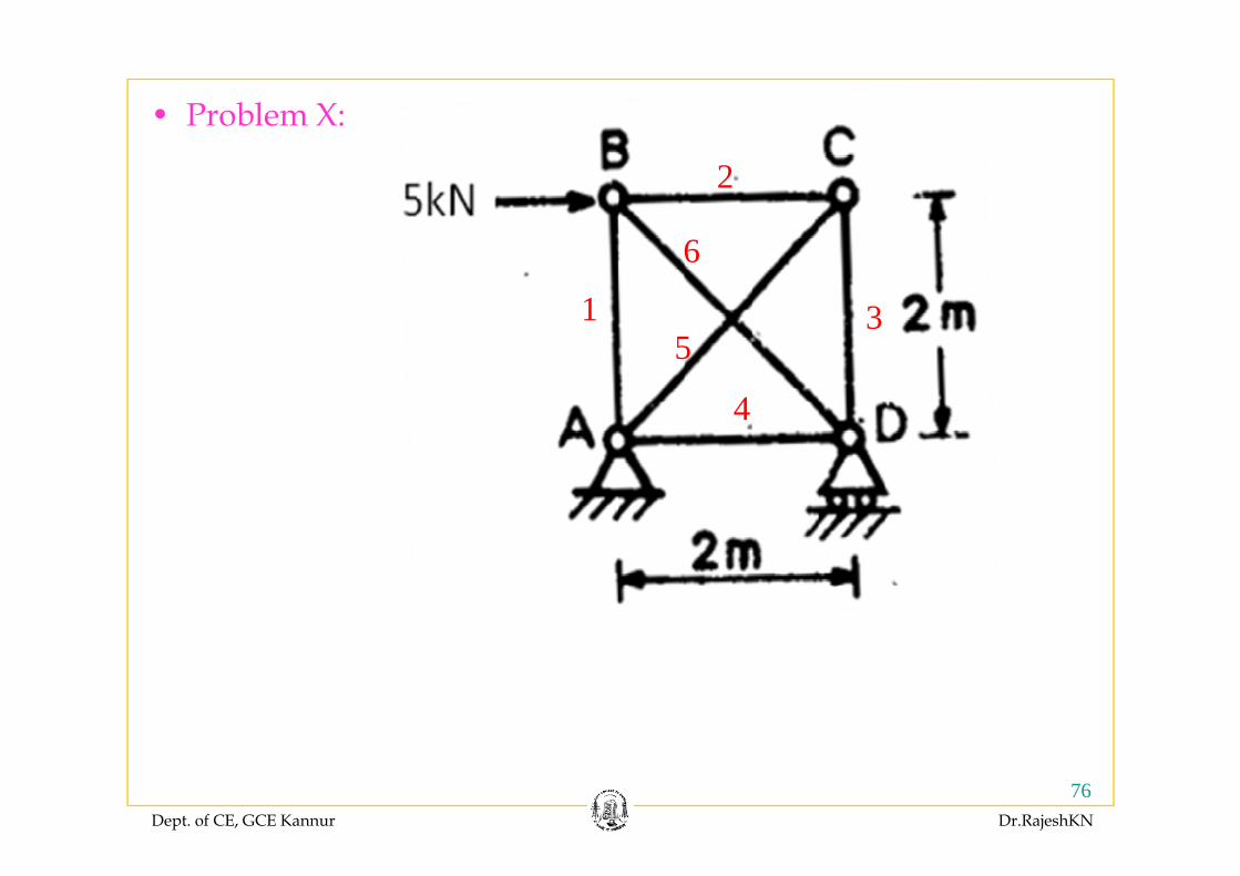
• Problem X:
2
6
1 35
6
4
5
Dept. of CE, GCE Kannur Dr.RajeshKN
76
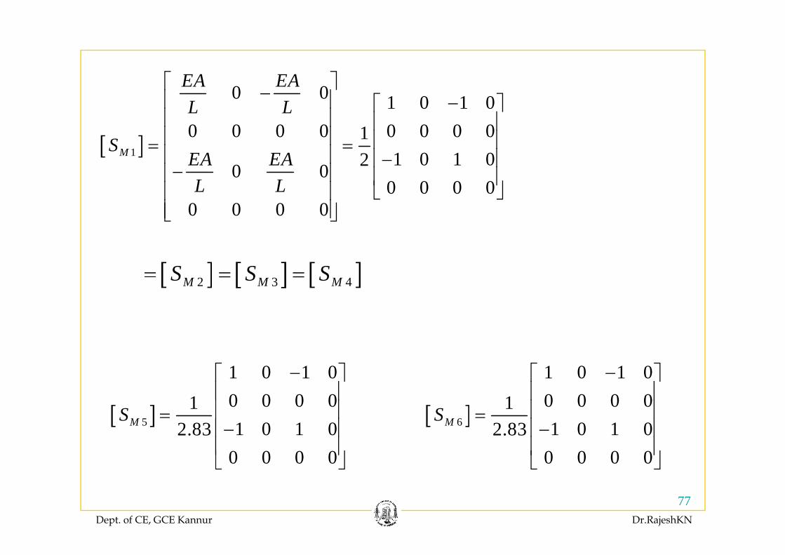
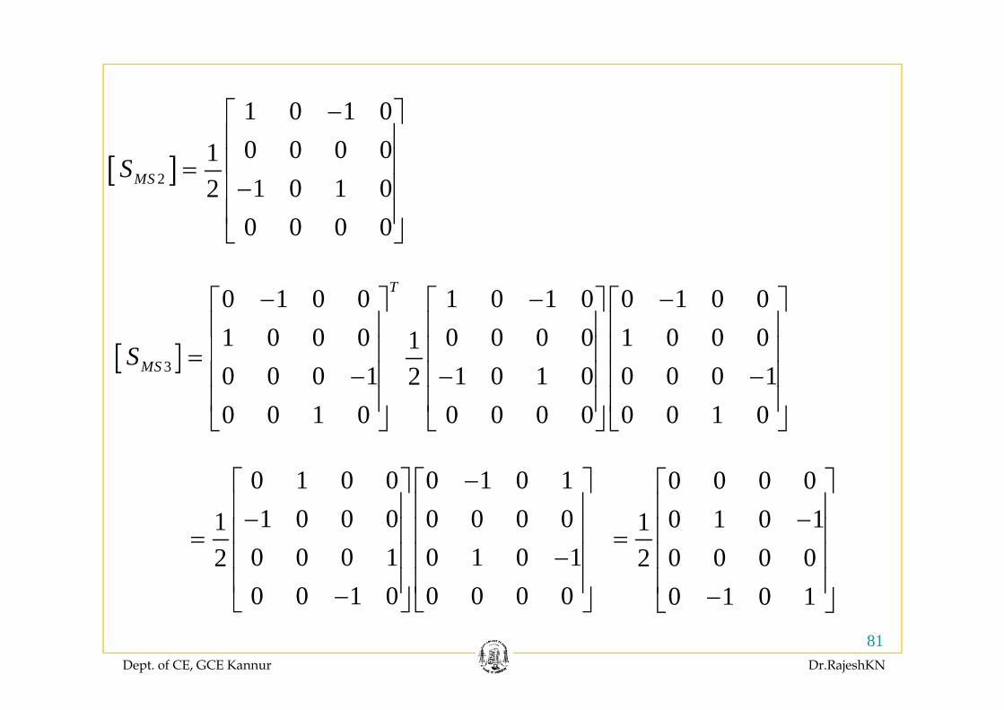
0 0EA EA⎡ ⎤
[ ]1
0 0 1 0 1 00 0 0 0 0 0 0 01
M
L L
S
⎡ ⎤−⎢ ⎥ −⎡ ⎤⎢ ⎥ ⎢ ⎥⎢ ⎥ ⎢ ⎥= =⎢ ⎥ ⎢ ⎥
[ ]1 1 0 1 020 00 0 0 0
0 0 0 0
M EA EAL L
⎢ ⎥ −⎢ ⎥−⎢ ⎥ ⎢ ⎥
⎣ ⎦⎢ ⎥⎢ ⎥⎣ ⎦0 0 0 0⎢ ⎥⎣ ⎦
[ ] [ ] [ ]2 3 4S S S= = =[ ] [ ] [ ]2 3 4M M MS S S
1 0 1 00 0 0 01
−⎡ ⎤⎢ ⎥⎢ ⎥
1 0 1 00 0 0 01
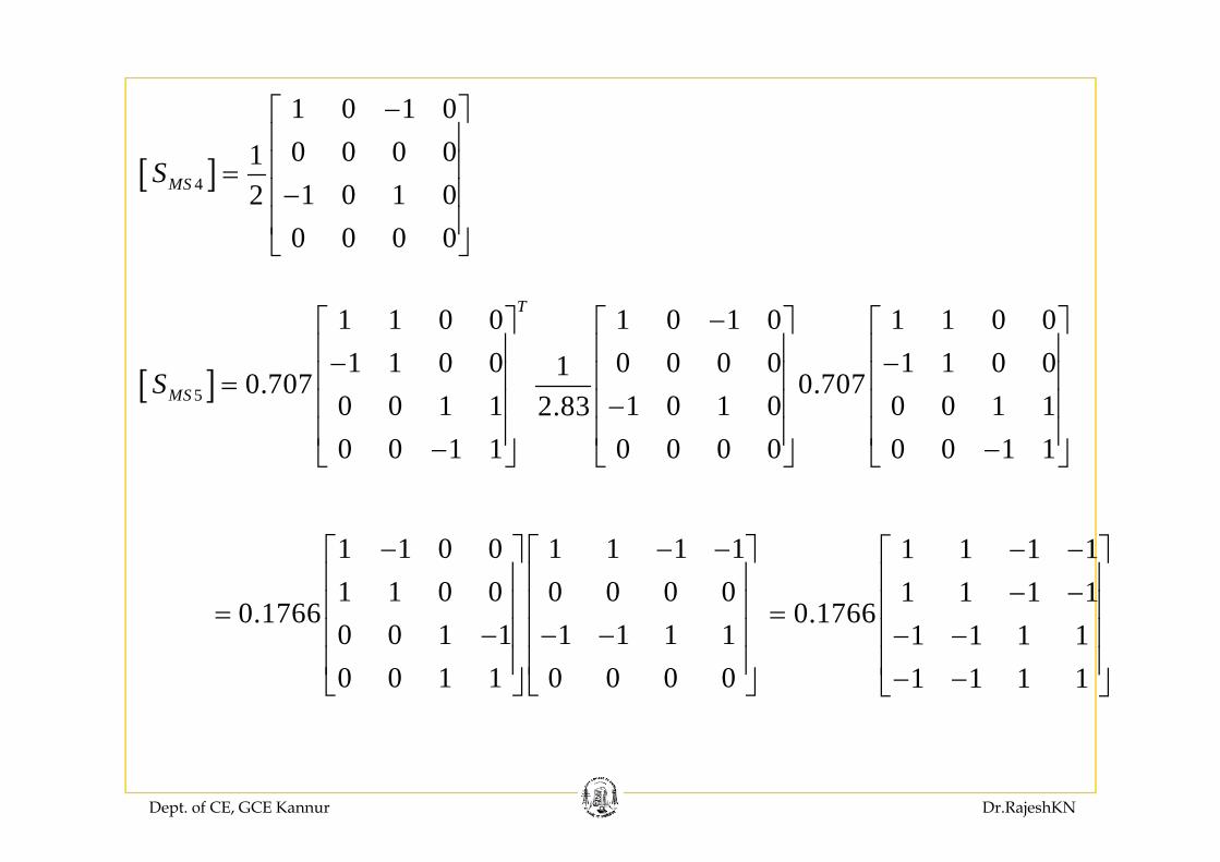
−⎡ ⎤⎢ ⎥⎢ ⎥[ ]5
0 0 0 011 0 1 02.83
0 0 0 0
MS ⎢ ⎥=−⎢ ⎥⎢ ⎥⎣ ⎦
[ ]6
0 0 0 011 0 1 02.83
0 0 0 0
MS ⎢ ⎥=−⎢ ⎥⎢ ⎥⎣ ⎦
Dept. of CE, GCE Kannur Dr.RajeshKN
77
⎣ ⎦ ⎣ ⎦
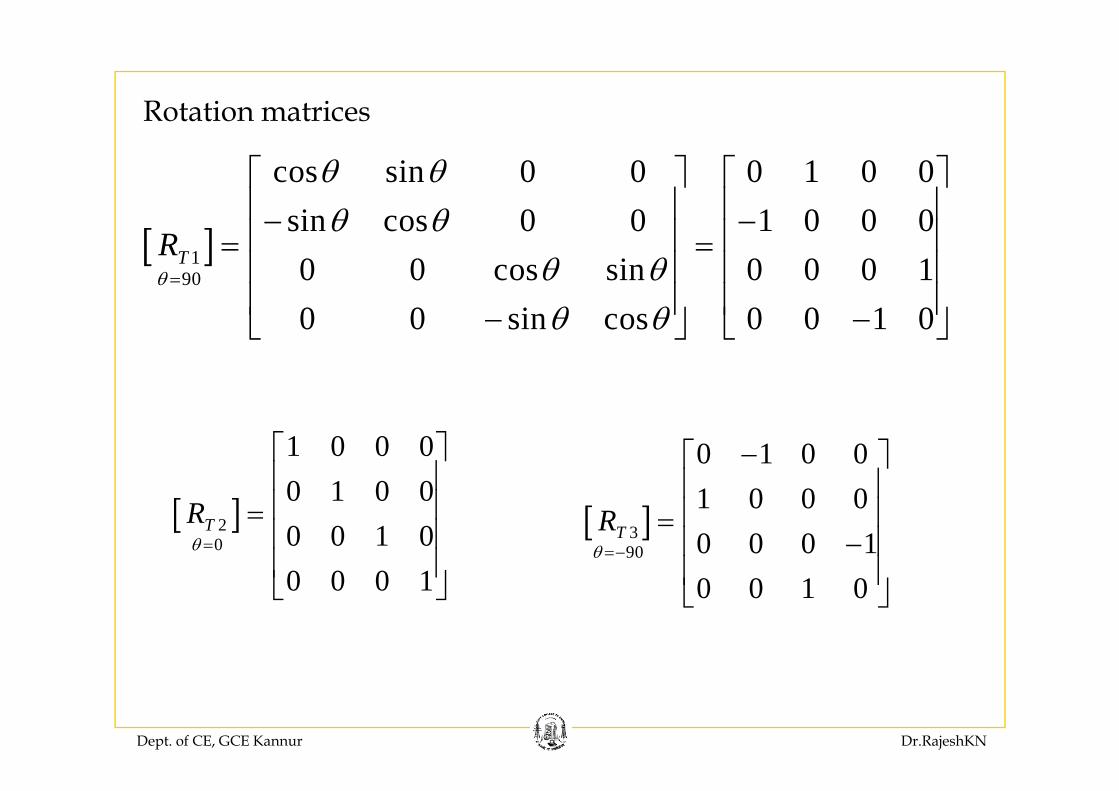
Rotation matrices
cos sin 0 0 0 1 0 0sin cos 0 0 1 0 0 0θ θθ θ
⎡ ⎤ ⎡ ⎤⎢ ⎥ ⎢ ⎥
[ ]190
sin cos 0 0 1 0 0 00 0 cos sin 0 0 0 1TR
θ
θ θθ θ=
⎢ ⎥ ⎢ ⎥− −⎢ ⎥ ⎢ ⎥= =⎢ ⎥ ⎢ ⎥⎢ ⎥ ⎢ ⎥0 0 sin cos 0 0 1 0θ θ⎢ ⎥ ⎢ ⎥− −⎣ ⎦ ⎣ ⎦
0 1 0 0−⎡ ⎤⎢ ⎥
1 0 0 00 1 0 0⎡ ⎤⎢ ⎥
[ ]390
1 0 0 00 0 0 1TR
θ =−
⎢ ⎥⎢ ⎥=
−⎢ ⎥⎢ ⎥
[ ]20
0 1 0 00 0 1 00 0 0 1
TRθ =
⎢ ⎥⎢ ⎥=⎢ ⎥⎢ ⎥⎣ ⎦ 0 0 1 0⎢ ⎥
⎣ ⎦0 0 0 1⎢ ⎥⎣ ⎦
Dept. of CE, GCE Kannur Dr.RajeshKN

[ ]
1 1 0 01 1 0 0
0 707R
⎡ ⎤⎢ ⎥−⎢ ⎥=[ ]
1 0 0 00 1 0 0
R
−⎡ ⎤⎢ ⎥−⎢ ⎥ [ ]5
450.707
0 0 1 10 0 1 1
TRθ =
⎢ ⎥=⎢ ⎥⎢ ⎥−⎣ ⎦
[ ]4180 0 0 1 0
0 0 0 1
TRθ =
⎢ ⎥=−⎢ ⎥
⎢ ⎥−⎣ ⎦⎣ ⎦
[ ]
1 1 0 01 1 0 0
−⎡ ⎤⎢ ⎥⎢ ⎥[ ]6
45
1 1 0 00.707
0 0 1 10 0 1 1
TRθ =−
⎢ ⎥=−⎢ ⎥
⎢ ⎥⎣ ⎦0 0 1 1⎣ ⎦
Dept. of CE, GCE Kannur Dr.RajeshKN
79
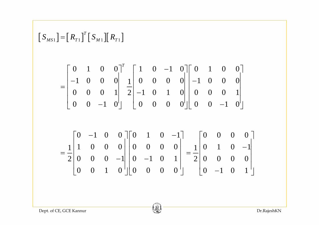
[ ] [ ] [ ][ ]TS R S R[ ] [ ] [ ][ ]1 1 1 1MS T M TS R S R=
0 1 0 0 1 0 1 0 0 1 0 01 0 0 0 0 0 0 0 1 0 0 01
T −⎡ ⎤ ⎡ ⎤ ⎡ ⎤⎢ ⎥ ⎢ ⎥ ⎢ ⎥− −⎢ ⎥ ⎢ ⎥ ⎢ ⎥=
0 0 0 1 1 0 1 0 0 0 0 120 0 1 0 0 0 0 0 0 0 1 0
⎢ ⎥ ⎢ ⎥ ⎢ ⎥=−⎢ ⎥ ⎢ ⎥ ⎢ ⎥
⎢ ⎥ ⎢ ⎥ ⎢ ⎥− −⎣ ⎦ ⎣ ⎦ ⎣ ⎦
0 0 0 0⎡ ⎤0 1 0 0 0 1 0 1− −⎡ ⎤ ⎡ ⎤0 1 0 110 0 0 02
⎡ ⎤⎢ ⎥−⎢ ⎥=⎢ ⎥⎢ ⎥
1 0 0 0 0 0 0 010 0 0 1 0 1 0 12
⎡ ⎤ ⎡ ⎤⎢ ⎥ ⎢ ⎥⎢ ⎥ ⎢ ⎥=
− −⎢ ⎥ ⎢ ⎥⎢ ⎥ ⎢ ⎥ 0 1 0 1⎢ ⎥−⎣ ⎦0 0 1 0 0 0 0 0⎢ ⎥ ⎢ ⎥⎣ ⎦ ⎣ ⎦
Dept. of CE, GCE Kannur Dr.RajeshKN
1 0 1 0−⎡ ⎤
[ ]2
1 0 1 00 0 0 011 0 1 02MSS
−⎡ ⎤⎢ ⎥⎢ ⎥=−⎢ ⎥1 0 1 020 0 0 0
⎢ ⎥⎢ ⎥⎣ ⎦
[ ]
0 1 0 0 1 0 1 0 0 1 0 01 0 0 0 0 0 0 0 1 0 0 01
T
S
− − −⎡ ⎤ ⎡ ⎤ ⎡ ⎤⎢ ⎥ ⎢ ⎥ ⎢ ⎥⎢ ⎥ ⎢ ⎥ ⎢ ⎥[ ]3 0 0 0 1 1 0 1 0 0 0 0 120 0 1 0 0 0 0 0 0 0 1 0
MSS ⎢ ⎥ ⎢ ⎥ ⎢ ⎥=− − −⎢ ⎥ ⎢ ⎥ ⎢ ⎥
⎢ ⎥ ⎢ ⎥ ⎢ ⎥⎣ ⎦ ⎣ ⎦ ⎣ ⎦
0 1 0 0 0 1 0 11 0 0 0 0 0 0 01
−⎡ ⎤ ⎡ ⎤⎢ ⎥ ⎢ ⎥
0 0 0 00 1 0 11⎡ ⎤⎢ ⎥1 0 0 0 0 0 0 01
0 0 0 1 0 1 0 120 0 1 0 0 0 0 0
⎢ ⎥ ⎢ ⎥−⎢ ⎥ ⎢ ⎥=−⎢ ⎥ ⎢ ⎥
⎢ ⎥ ⎢ ⎥⎣ ⎦ ⎣ ⎦
0 1 0 110 0 0 020 1 0 1
⎢ ⎥−⎢ ⎥=⎢ ⎥⎢ ⎥⎣ ⎦
Dept. of CE, GCE Kannur Dr.RajeshKN
81
0 0 1 0 0 0 0 0−⎣ ⎦ ⎣ ⎦ 0 1 0 1−⎣ ⎦
1 0 1 0−⎡ ⎤⎢ ⎥
[ ]4
0 0 0 011 0 1 02
0 0 0 0
MSS⎢ ⎥⎢ ⎥=−⎢ ⎥⎢ ⎥⎣ ⎦0 0 0 0⎣ ⎦
1 1 0 0 1 0 1 0 1 1 0 0T −⎡ ⎤ ⎡ ⎤ ⎡ ⎤⎢ ⎥ ⎢ ⎥ ⎢ ⎥
[ ]5
1 1 0 0 0 0 0 0 1 1 0 010.707 0.7070 0 1 1 1 0 1 0 0 0 1 12.83MSS
⎡ ⎤ ⎡ ⎤ ⎡ ⎤⎢ ⎥ ⎢ ⎥ ⎢ ⎥− −⎢ ⎥ ⎢ ⎥ ⎢ ⎥=
−⎢ ⎥ ⎢ ⎥ ⎢ ⎥⎢ ⎥ ⎢ ⎥ ⎢ ⎥0 0 1 1 0 0 0 0 0 0 1 1⎢ ⎥ ⎢ ⎥ ⎢ ⎥− −⎣ ⎦ ⎣ ⎦ ⎣ ⎦
1 1 0 0 1 1 1 11 1 0 0 0 0 0 0
0.17660 0 1 1 1 1 1 1
− − −⎡ ⎤ ⎡ ⎤⎢ ⎥ ⎢ ⎥⎢ ⎥ ⎢ ⎥=⎢ ⎥ ⎢ ⎥
1 1 1 11 1 1 1
0.17661 1 1 1
− −⎡ ⎤⎢ ⎥− −⎢ ⎥=⎢ ⎥0 0 1 1 1 1 1 1
0 0 1 1 0 0 0 0− − −⎢ ⎥ ⎢ ⎥
⎢ ⎥ ⎢ ⎥⎣ ⎦ ⎣ ⎦
1 1 1 11 1 1 1
− −⎢ ⎥⎢ ⎥− −⎣ ⎦
Dept. of CE, GCE Kannur Dr.RajeshKN
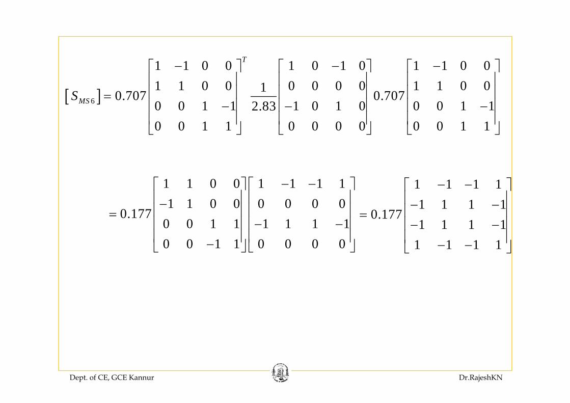
1 1 0 0 1 0 1 0 1 1 0 0T⎡ ⎤ ⎡ ⎤ ⎡ ⎤
[ ]6
1 1 0 0 1 0 1 0 1 1 0 01 1 0 0 0 0 0 0 1 1 0 010.707 0.7070 0 1 1 1 0 1 0 0 0 1 12.83MSS
− − −⎡ ⎤ ⎡ ⎤ ⎡ ⎤⎢ ⎥ ⎢ ⎥ ⎢ ⎥⎢ ⎥ ⎢ ⎥ ⎢ ⎥=
− − −⎢ ⎥ ⎢ ⎥ ⎢ ⎥0 0 1 1 1 0 1 0 0 0 1 12.830 0 1 1 0 0 0 0 0 0 1 1⎢ ⎥ ⎢ ⎥ ⎢ ⎥⎢ ⎥ ⎢ ⎥ ⎢ ⎥⎣ ⎦ ⎣ ⎦ ⎣ ⎦
1 1 1 11 1 1 1
− −⎡ ⎤⎢ ⎥
1 1 0 0 1 1 1 11 1 0 0 0 0 0 0
− −⎡ ⎤ ⎡ ⎤⎢ ⎥ ⎢ ⎥ 1 1 1 1
0.1771 1 1 1
1 1 1 1
⎢ ⎥− −⎢ ⎥=− −⎢ ⎥⎢ ⎥− −⎣ ⎦
1 1 0 0 0 0 0 00.177
0 0 1 1 1 1 1 10 0 1 1 0 0 0 0
⎢ ⎥ ⎢ ⎥−⎢ ⎥ ⎢ ⎥=− −⎢ ⎥ ⎢ ⎥
⎢ ⎥ ⎢ ⎥−⎣ ⎦ ⎣ ⎦ 1 1 1 1⎣ ⎦0 0 1 1 0 0 0 0⎣ ⎦ ⎣ ⎦
Dept. of CE, GCE Kannur Dr.RajeshKN
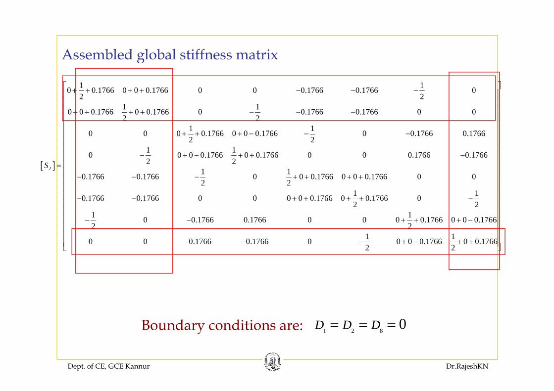
Assembled global stiffness matrix
1 10 0.1766 0 0 0.1766 0 0 0.1766 0.1766 02 2
1 1
+ + + + − − −⎡ ⎤⎢ ⎥⎢ ⎥⎢ ⎥
g
1 10 0 0.1766 0 0.1766 0 0.1766 0.1766 0 02 2
1 10 0 0 0.1766 0 0 0.1766 0 0.1766 0.17662 2
1 1
+ + + + − − −
+ + + − − −
⎢ ⎥⎢ ⎥⎢ ⎥⎢ ⎥⎢ ⎥⎢ ⎥
[ ]1 10 0 0 0.1766 0 0.1766 0 0 0.1766 0.17662 2
1 10.1766 0.1766 0 0 0.1766 0 0 0.2 2
JS− + − + + −
=− − − + + + + 1766 0 0
1 10 1766 0 1766 0 0 0 0 0 1766 0 0 1766 0
⎢ ⎥⎢ ⎥⎢ ⎥⎢ ⎥⎢ ⎥⎢ ⎥⎢ ⎥1 10.1766 0.1766 0 0 0 0 0.1766 0 0.1766 0
2 21 10 0.1766 0.1766 0 0 0 0.1766 0 0 0.17662 2
1 10 0 0 1766 0 1766 0 0 0 0 1766 0 0 1766
⎢ ⎥− − + + + + −⎢ ⎥⎢ ⎥⎢ − − + + + − ⎥⎢ ⎥⎢ ⎥
+ + +⎢ ⎥0 0 0.1766 0.1766 0 0 0 0.1766 0 0.17662 2
− − + − + +⎢ ⎥⎣ ⎦
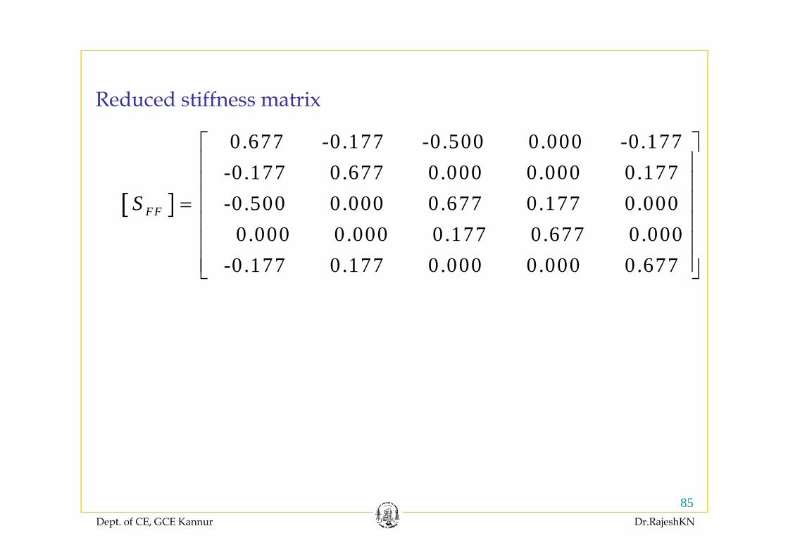
1 2 8 0D D D= = =Boundary conditions are:
Dept. of CE, GCE Kannur Dr.RajeshKN
1 2 8 0D D DBoundary conditions are:
0 .677 -0 .177 -0 .500 0 .000 -0 .177 ⎡ ⎤⎢ ⎥
Reduced stiffness matrix
[ ] -0.177 0 .677 0 .000 0 .000 0 .177 -0.500 0 .000 0 .677 0 .177 0 .000FFS =
⎢ ⎥⎢ ⎥⎢ ⎥⎢ ⎥
[ ] 0 .000 0 .000 0 .177 0 .677 0 .000 -0.177 0 .177 0 .000 0 .000 0 .677
⎢ ⎥⎢ ⎥⎢ ⎥⎣ ⎦⎣ ⎦
Dept. of CE, GCE Kannur Dr.RajeshKN
85
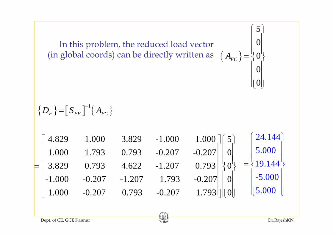
5⎧ ⎫⎪ ⎪
{ }00FCA
⎪ ⎪⎪ ⎪⎪ ⎪= ⎨ ⎬⎪ ⎪
In this problem, the reduced load vector (in global coords) can be directly written as
00
⎪ ⎪⎪ ⎪⎪ ⎪⎩ ⎭
{ } [ ] { }1F FF FCD S A−=
24.144⎧ ⎫⎪ ⎪
4.829 1.000 3.829 -1.000 1.000 5⎡ ⎤ ⎧ ⎫⎢ ⎥ ⎪ ⎪ 5.000
19.144
⎪ ⎪⎪ ⎪⎪ ⎪⎨ ⎬⎪
=⎪
1.000 1.793 0.793 -0.207 -0.207 3.829 0.793 4.622 -1.207 0.793=
00
⎢ ⎥ ⎪ ⎪⎢ ⎥ ⎪ ⎪⎪ ⎪⎢ ⎥ ⎨ ⎬⎢ ⎥ ⎪ ⎪ -5.000
5.000
⎪⎪⎪
⎪⎪⎪⎩ ⎭
-1.000 -0.207 -1.207 1.793 -0.207 0 1.000 -0.207 0.793 -0.207 1.793 0
⎢ ⎥ ⎪ ⎪⎢ ⎥ ⎪ ⎪⎢ ⎥ ⎪ ⎪⎣ ⎦ ⎩ ⎭
Dept. of CE, GCE Kannur Dr.RajeshKN
⎣ ⎦ ⎩ ⎭
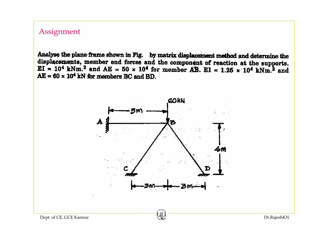
Assignment
Dept. of CE, GCE Kannur Dr.RajeshKN