MODULE : NON-SYMMETRICAL AND INHOMOGENEOUS...
100
STRUCTURAL MECHANICS 4 CIE3109 MODULE : NON-SYMMETRICAL AND INHOMOGENEOUS CROSS SECTIONS COEN HARTSUIJKER HANS WELLEMAN Civil Engineering TU-Delft October 2017
Transcript of MODULE : NON-SYMMETRICAL AND INHOMOGENEOUS...

STRUCTURAL MECHANICS 4 CIE3109
MODULE : NON-SYMMETRICAL AND INHOMOGENEOUS CROSS SECTIONS
COEN HARTSUIJKER HANS WELLEMAN Civil Engineering TU-Delft
October 2017

STRUCTURAL MECHANICS 4 Non-symmetrical and inhomogeneous cross sections
Ir C. Hartsuijker & Ir J.W. Welleman October 2017 ii
TABLE of CONTENTS
1. NON-SYMMETRICAL AND INHOMOGENEOUS CROSS SECTIONS ........................................... 1
1.1 SKETCH OF THE PROBLEM AND REQUIRED ASSUMPTIONS .......................................................................... 1
1.2 HOMOGENEOUS CROSS SECTIONS .............................................................................................................. 4
1.2.1 Kinematic relations ......................................................................................................................... 4
1.2.1.1 Curvature .................................................................................................................................................... 6
1.2.1.2 Neutral axis ................................................................................................................................................. 7
1.2.2 Constitutive relations for homogeneous non-symmetrical cross sections ....................................... 8
1.2.2.1 Moments ................................................................................................................................................... 10
1.2.2.2 Properties of the constitutive relation for bending .................................................................................... 11
1.2.3 Equilibrium conditions .................................................................................................................. 13
1.2.4 Differential Equations ................................................................................................................... 14
1.2.5 Example 1 : Homogeneous non-symmetrical cross section .......................................................... 15
1.2.6 Normal stresses in the y-z-coordinate system ............................................................................... 19
1.2.7 Normal stresses in the principal coordinate system ...................................................................... 20
1.2.8 Example 2 : Stresses in non-symmetrical cross sections ............................................................... 21
1.2.9 Concluding remarks ...................................................................................................................... 27
1.3 EXTENSION OF THE THEORY FOR INHOMOGENEOUS CROSS SECTIONS ...................................................... 28
1.3.1 Position of the NC for inhomogeneous cross sections .................................................................. 31
1.3.2 Example 3 : Normal centre versus centroid .................................................................................. 32
1.3.3 Example 4 : Stresses in inhomogeneous cross sections ................................................................ 33
1.4 FORCE POINT OF THE CROSS SECTION ...................................................................................................... 36
1.5 CORE OR KERN OF A CROSS SECTION ....................................................................................................... 38
1.5.1 Example 5 : Core of a non-symmetrical cross section .................................................................. 42
1.6 TEMPERATURE INFLUENCES* .................................................................................................................. 44
1.6.1 Example 6 : Static determinate structure under temperature load ............................................... 47
1.6.2 Example 7 : Static indeterminate structure under temperature load ............................................ 51
1.7 SHEAR STRESS DISTRIBUTION IN ARBITRARY CROSS SECTIONS ................................................................ 55
1.7.1 Shear stress equations for principal coordinate systems .............................................................. 56
1.7.1.1 Example 8 : Shear stresses in a composite cross section .......................................................................... 58
1.7.2 General shear stress formula ........................................................................................................ 59
1.7.2.1 Example 9 : Shear stresses in a non-symmetrical cross section ................................................................ 60
1.7.2.2 Example 10 : Shear force in a non homogeneous cross section ................................................................ 66
1.7.3 Shear force center for thin walled non-symmeyrical cross sections ............................................. 68
1.7.3.1 Example 11 : Shear force center for thin walled cross sections ................................................................ 69
APPENDIX A ...................................................................................................................................................... 75
APPENDIX B ...................................................................................................................................................... 77
2. ASSIGNMENTS ........................................................................................................................................ 79
2.1 CROSS SECTIONAL PROPERTIES ................................................................................................................ 79
2.2 NORMAL STRESSES IN CASE OF BENDING ................................................................................................. 82
2.3 NORMAL STRESSES DUE TO BENDING AND EXTENSION ............................................................................ 87
2.4 INHOMOGENEOUS CROSS SECTIONS LOADED IN EXTENSION..................................................................... 89
2.5 INHOMOGENEOUS CROSS SECTIONS LOADED IN BENDING ........................................................................ 90
2.6 CORE ....................................................................................................................................................... 93
2.7 SHEAR STRESSES DUE TO BENDING .......................................................................................................... 96
STRUCTURAL MECHANICS 4 Non-symmetrical and inhomogeneous cross sections
Ir C. Hartsuijker & Ir J.W. Welleman October 2017 iii
STUDY GUIDE
These lecture notes are part of the course CIE3109 Structural Mechanics 4 (CM4). Both
theory and examples are presented for self-study. Additional study material is available via
the internet. Sheets used and additional comments made in the lectures are available via
BlackBoard or also via internet:
http://icozct.tudelft.nl/TUD_CT/
In these notes reference is made to the first year lecture notes of Structural Mechanics 1 and
Structural Mechanics 2 and Structural Mechanics 3 which are covered with three books:
o Engineering Mechanics, volume 1 : Equilibrium, C. Hartsuijker and J.W. Welleman
o Engineering Mechanics, volume 2 : Stresses, strains and displacements C. Hartsuijker and J.W.
Welleman
o Toegepaste Mechanica , deel 3 : Statisch onbepaalde constructies en bezwijkanalyse, C.
Hartsuijker en J.W. Welleman (in Dutch)
These books will be referred to as MECH-1, MECH-2 and MECH-3.
The answers to the assignments can be found via the above mentioned web site. If needed
additional information can be obtained from the Student Assistants of Structural Mechanics.
Although these notes have been prepared with the utmost precision faults can not be
excluded. I will appreciate any comments made and invite students to read the material
carefully and make suggestions for improvement. Any reported faults will be printed on the
internet site to inform all students.
The lecturer,
Hans Welleman
pdf-edition nr 11-3, October 2017

STRUCTURAL MECHANICS 4 Non-symmetrical and inhomogeneous cross sections
Ir C. Hartsuijker & Ir J.W. Welleman October 2017 1
1. NON-SYMMETRICAL AND INHOMOGENEOUS CROSS SECTIONS
In this module the in MECH-2 introduced fiber model for beams will be extended and used on beams with a non-symmetrical and/or inhomogeneous cross section. With the presented theory a straight forward and easy method is obtained to calculate the stresses and strains in cross sections made out of different materials (inhomogeneous) and or with no axis of symmetry (non-symmetrical).
1.1 Sketch of the problem and required assumptions
The cross sections used so far, always contained at least one axis of symmetry and the cross
section itself was always made out of one single material (homogeneous cross section). With
the fiber model as introduced in MECH-2 the cross section is modeled as a collection of
initially straight fibers which are parallel to the beam axis denoted as x-axis. The fibers are
kept together by infinite rigid cross sections which are by definition perpendicular to the beam
axis. In figure 1 this model is shown together with the coordinate system used. The origin of
the coordinate system of the cross section is the Normal Centre NC. A detailed description of
this model can be found in chapter 4 of MECH-21.
Figure 1 : Fiber model and a cross section with one axis of symmetry.
If a cross section is loaded with one single bending moment and a normal force, all fibers at
the tensile side will elongate and fibers at the compressive side will shorten. Due to the
assumption of the infinite rigidity of the cross section the plane cross sections will remain
plain. This is known as the hypothesis of Bernoulli. In figure 2a all sectional forces are shown
and in figure 2b the resulting strains in the fibers are shown. If a linear relation between
strains and stresses is assumed (Hooke’s law) the resulting normal stresses due to combined
bending and normal force can be presented as is shown in figure 2c .
(a) (b) (c)
Figure 2 : Bending and extension in a homogeneous cross section with one axis of symmetry.
1 C. Hartsuijker and J.W. Welleman, Engineering Mechanics, Volume 2, ISBN 9039505942
N
fiber
fiber
beam axis
axis of symmetry cross sections

STRUCTURAL MECHANICS 4 Non-symmetrical and inhomogeneous cross sections
Ir C. Hartsuijker & Ir J.W. Welleman October 2017 2
Based on this model, formulas for calculating stresses for combined bending and extension,
have been found in MECH-2. For non-symmetrical and or inhomogeneous cross sections the
found formulas can not be used. Examples of these situations are given in figure 3.
Figure 3 : Examples of non-symmetrical and/or inhomogeneous cross sections.
Example (a) shows a non-symmetrical cross section. In (b) the cross section is
inhomogeneous with one axis of symmetry. In (c) the cross section is inhomogeneous and
non-symmetrical. Apart from the shape and material of the cross section also the loading of
the cross section is important. In general a cross section can be loaded with three forces (two
shear forces and one normal force) and three moments (two bending moments and one
trosional moment). The fiber model only describes the strains and stresses due to bending and
extension. The influence of the shear forces and torsional moments are therefore excluded.
The definitions used for the normal force, bending moments and the displacements as
introduced in section 1.3.2 of MECH-1 are shown in figure 4, see also section 1.2.2.
Figure 4 : Sectional forces and displacements.
The shear forces will not cause any strains in the fiber model. However with a simple model
as introduced in MECH-2 we can obtain the shear stresses due to shear forces. At the end of
these lecture notes a special chapter deals with the subject of shear stresses and the shear
centre SC.
For this chapter the central question to answer is :
‘How to describe the strains and stresses in non-symmetrical and/or inhomogeneous cross
section due to the combined loading of bending and extension’ ?
In order to answer this question in a structured way we can split the question in a number of
sub questions:
• How can we find the strains due to the displacements of the cross section ?
• How can we find the (normal) stresses due to the strains in the fibers ?
• How can we find the (cross) sectional forces which belong to these (normal) stresses ?
z
z z
y
y
y
(a) (b) (c)
concrete
steel
E1
E1
E2
ux
uz uy x
z
y
Fz
Fx Fy
F
ϕz
ϕx ϕy
STRUCTURAL MECHANICS 4 Non-symmetrical and inhomogeneous cross sections
Ir C. Hartsuijker & Ir J.W. Welleman October 2017 3
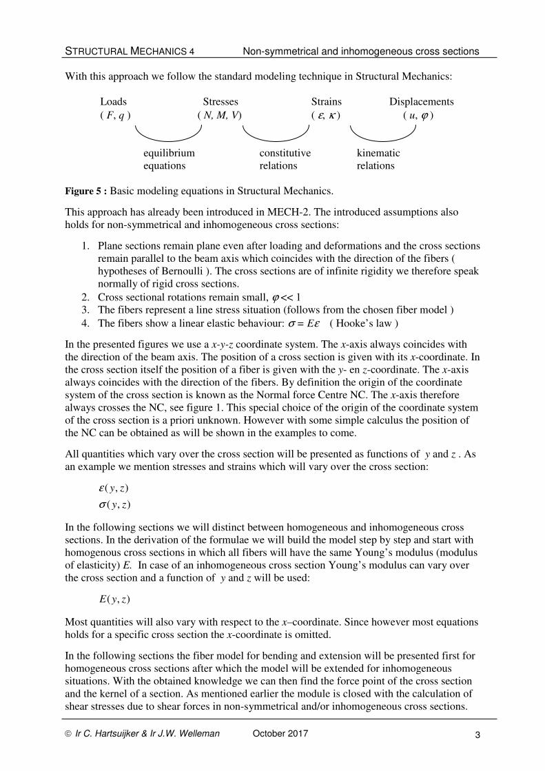
With this approach we follow the standard modeling technique in Structural Mechanics:
Loads Stresses Strains Displacements
( F, q ) ( N, M, V) ( ε, κ ) ( u, ϕ )
equilibrium constitutive kinematic
equations relations relations
Figure 5 : Basic modeling equations in Structural Mechanics.
This approach has already been introduced in MECH-2. The introduced assumptions also
holds for non-symmetrical and inhomogeneous cross sections:
1. Plane sections remain plane even after loading and deformations and the cross sections
remain parallel to the beam axis which coincides with the direction of the fibers (
hypotheses of Bernoulli ). The cross sections are of infinite rigidity we therefore speak
normally of rigid cross sections.
2. Cross sectional rotations remain small, ϕ << 1
3. The fibers represent a line stress situation (follows from the chosen fiber model )
4. The fibers show a linear elastic behaviour: σ = Eε ( Hooke’s law )
In the presented figures we use a x-y-z coordinate system. The x-axis always coincides with
the direction of the beam axis. The position of a cross section is given with its x-coordinate. In
the cross section itself the position of a fiber is given with the y- en z-coordinate. The x-axis
always coincides with the direction of the fibers. By definition the origin of the coordinate
system of the cross section is known as the Normal force Centre NC. The x-axis therefore
always crosses the NC, see figure 1. This special choice of the origin of the coordinate system
of the cross section is a priori unknown. However with some simple calculus the position of
the NC can be obtained as will be shown in the examples to come.
All quantities which vary over the cross section will be presented as functions of y and z . As
an example we mention stresses and strains which will vary over the cross section:
),(
),(
zy
zy
σ
ε
In the following sections we will distinct between homogeneous and inhomogeneous cross
sections. In the derivation of the formulae we will build the model step by step and start with
homogenous cross sections in which all fibers will have the same Young’s modulus (modulus
of elasticity) E. In case of an inhomogeneous cross section Young’s modulus can vary over
the cross section and a function of y and z will be used:
),( zyE
Most quantities will also vary with respect to the x–coordinate. Since however most equations
holds for a specific cross section the x-coordinate is omitted.
In the following sections the fiber model for bending and extension will be presented first for
homogeneous cross sections after which the model will be extended for inhomogeneous
situations. With the obtained knowledge we can then find the force point of the cross section
and the kernel of a section. As mentioned earlier the module is closed with the calculation of
shear stresses due to shear forces in non-symmetrical and/or inhomogeneous cross sections.

STRUCTURAL MECHANICS 4 Non-symmetrical and inhomogeneous cross sections
Ir C. Hartsuijker & Ir J.W. Welleman October 2017 4
1.2 Homogeneous cross sections
The modeling steps of figure 5 will be elaborated this section. We will start with
homogeneous cross sections which can be non symmetrical.
1.2.1 Kinematic relations
The kinematic relations relate the displacements of a cross section to the fiber strains in the
cross section. A cross section loaded in combined bending and extension may exhibit three
translations and three rotations :
zyxzyx ,,en,, ϕϕϕuuu
We will use the earlier introduced definitions of the displacements, see figure 4.
If the displacement of the cross section can be described with these six degrees of freedom
then we can also describe the displacement u in the x-direction of any fiber in the cross
section. Suppose point P(x,y,z) is in the cross section at a distance x of the beams origin, see
figure 6.
Figure 6 : Point P(x,y,z) in a cross section at distance x from the origin.
The cross section moves with ux in x-direction and rotates with ϕy along the y-axis and with
ϕz along the z-axis. The displacement u in the direction of the fiber at P can be written with
the assumption of small rotations (see section 15.3.2 from MECH-l) as:
yzx),,( ϕϕ zyuzyxu +−=
In figure 7 this is clarified with some sketches of the displaced cross section (dashed) which is
subsequently rotated along the y- and z-axis. Both the top and side view show the influence of
the rotations upon the displacement u.
Figure 7 : Displacement in the direction of the fibers due to the rotations ϕy en ϕz.
x
y
z
ux
x
y
x
z
top view side view
P yϕz y
zϕy z
fiber
cross section
STRUCTURAL MECHANICS 4 Non-symmetrical and inhomogeneous cross sections
Ir C. Hartsuijker & Ir J.W. Welleman October 2017 5
Due to the assumed small rotations the influences in the displacement can be superposed. The
displacement quantities ux , ϕy en ϕz belong to the cross section which contains P and are
therefore cross sectional related quantities. These displacements are thus only functions of x.
In other words: the displacements of an arbitrary fiber in a cross section at a distance x can be
described with three displacements quantities.
With the displacement of a point P also the straining of a fiber through P can be obtained. The
relative displacement which is known as the engineering strain of a fiber can be found with:
yzx
yzx
0
),(
),,(),,(lim),(
ϕϕε
ϕϕε
′+′−′=
+−=∂
∂=
∆
∆=
→∆
zyuzy
dx
dz
dx
dy
dx
du
x
zyxu
x
zyxuzy
x (a)
The rotations ϕy en ϕz can be expressed in the displacement quantities uy en uz. See figure 7.
y
y
z
zz
y
d
d
d
d
ux
u
ux
u
′=+=
′−=−=
ϕ
ϕ
The change in sign is due to the definitions of the rotations ( check this yourself !).
The strain according to (a) in the fiber through P can be written as:
zyx),( uzuyuzy ′′−′′−′=ε (b)
The strain of the beam axis is equal to the strain of the fiber through the x-axis added with the
strain due to bending (curvature) along the y- and z-axis. Expression (b) can be rewritten with
the introduction of the following three cross sectional deformation quantities:
yzz
zyy
x
ϕκ
ϕκ
ε
′=′′−=
′−=′′−=
′=
u
u
u
(c)
These relations are known as the kinematic relations
and relate the cross sectional deformation quantities
to the cross sectional displacement quantities.
With the kinematic relations (c) the strain in a fiber
according to (b) can be written as:
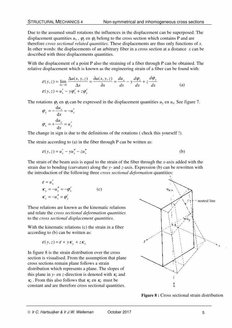
zy),( κκεε zyzy ++=
In figure 8 is the strain distribution over the cross
section is visualised. From the assumption that plane
cross sections remain plane follows a strain
distribution which represents a plane. The slopes of
this plane in y- en z-direction is denoted with κy and
κz . From this also follows that κy en κz must be
constant and are therefore cross sectional quantities.
Figure 8 : Cross sectional strain distribution
neutral line
STRUCTURAL MECHANICS 4 Non-symmetrical and inhomogeneous cross sections
Ir C. Hartsuijker & Ir J.W. Welleman October 2017 6
From figure 8 also follows that positive curvatures causes for positive values of y and z
positive strains. This is in complete agreement with the definition of positive curvatures as
introduced in MECH-2.
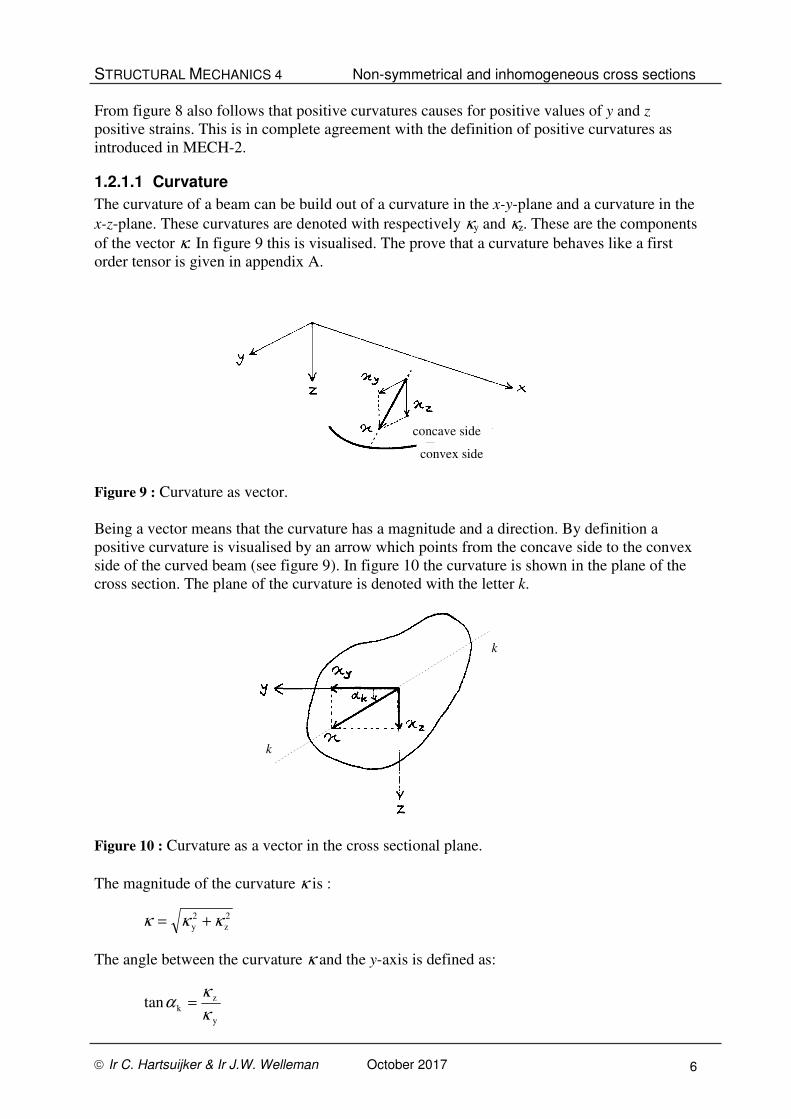
1.2.1.1 Curvature
The curvature of a beam can be build out of a curvature in the x-y-plane and a curvature in the
x-z-plane. These curvatures are denoted with respectively κy and κz. These are the components
of the vector κ. In figure 9 this is visualised. The prove that a curvature behaves like a first
order tensor is given in appendix A.
Figure 9 : Curvature as vector.
Being a vector means that the curvature has a magnitude and a direction. By definition a
positive curvature is visualised by an arrow which points from the concave side to the convex
side of the curved beam (see figure 9). In figure 10 the curvature is shown in the plane of the
cross section. The plane of the curvature is denoted with the letter k.
Figure 10 : Curvature as a vector in the cross sectional plane.
The magnitude of the curvature κ is :
2
z
2
y κκκ +=
The angle between the curvature κ and the y-axis is defined as:
y
zktan
κ
κα =
k
k
convex side
concave side

STRUCTURAL MECHANICS 4 Non-symmetrical and inhomogeneous cross sections
Ir C. Hartsuijker & Ir J.W. Welleman October 2017 7
1.2.1.2 Neutral axis
With the expression of the strain distribution over the cross section, we can also find an
expression for fibers with zero strain. The fibers in the cross section with zero strains form a
line which is called the neutral line or neutral axis. In order to keep in line with the Dutch
edition of these notes we will use neutral line which is abbreviated as nl. With the zero strain
definition the expression for the neutral line becomes:
0),( zy =++= κκεε zyzy
In order to draw the neutral line in the cross section, two handy points are needed. These
points are the points of intersection with the coordinate axis. The neutral line crosses the
coordinate axis in:
Point of intersection with the y-axis (z = 0) : yκ
ε−=y
Point of intersection with the z-axis (y = 0): zκ
ε−=z
In figure 11 the neutral axis is drawn in the cross sectional coordinate system.
Figuur 11 : Position of the neutral line in the cross section.
This figure also shows that the beam’s plane of curvature k is perpendicular to the neutral
axis. The arrow representing the curvature directs from the concave (smallest strain) to the
convex (largest strain) side. In this case from the compressive zone in to the tensile zone.
Assignment:
Give the proof for the observation that the plane of curvature is perpendicular to the neutral
line.
k
neutral line nl.
STRUCTURAL MECHANICS 4 Non-symmetrical and inhomogeneous cross sections
Ir C. Hartsuijker & Ir J.W. Welleman October 2017 8
1.2.2 Constitutive relations for homogeneous non-symmetrical cross sections
The fiber model used so far, assumes a linear elastic stress-strain relation. We will restrict
ourselves to this simple model, using Hooke’s law:
εσ ×= E
In a cross section the strain and stress in a certain point is denoted with respect to the chosen
coordinate system:
),();,( zyzy εεσσ ==
In case of a homogeneous cross section all fibers will have the same Young’s modulus E. The
stress in a certain point can easily be found from the computed strains with:
),(),( zyEzy εσ ×=
In combined loaded sections (bending and extension), fibers will lengthen or shorten. The
deformation behaviour of a particular cross section can be described with the earlier
introduced three cross sectional deformation quantities:
zy en, κκε
The strain in any fiber (y,z) at the cross section is now known with:
zy),( κκεε zyzy ++=
Using Hooke’s law for the stress strain relation we can find the expression for the stress in
any particular (fiber) point of the cross section:
( )zy),( κκεσ zyEzy ++×=
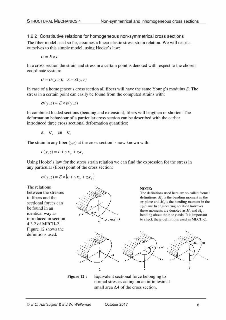
The relations
between the stresses
in fibers and the
sectional forces can
be found in an
identical way as
introduced in section
4.3.2 of MECH-2.
Figure 12 shows the
definitions used.
Figure 12 : Equivalent sectional force belonging to
normal stresses acting on an infinitesimal
small area ∆A of the cross section.
NOTE:
The definitions used here are so called formal
definitions. My is the bending moment in the
xy-plane and Mz is the bending moment in the
xz-plane In engineering notation however
these moments are denoted as Mz and My ,
bending about the z or y axis. It is important
to check these definitions used in MECH-2.
STRUCTURAL MECHANICS 4 Non-symmetrical and inhomogeneous cross sections
Ir C. Hartsuijker & Ir J.W. Welleman October 2017 9
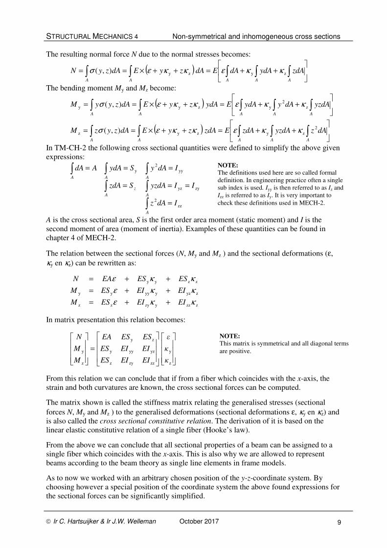
The resulting normal force N due to the normal stresses becomes:
( )
++=++×== ∫ ∫∫∫∫
A AAAA
zdAydAdAEdAzyEdAzyN zyzy),( κκεκκεσ
The bending moment My and Mz become:
( )
( )
++=++×==
++=++×==
∫ ∫∫∫∫
∫ ∫∫∫∫
A AAAA
A AAAA
dAzyzdAzdAEzdAzyEdAzyzM
yzdAdAyydAEydAzyEdAzyyM
2
zyzyz
z
2
yzyy
),(
),(
κκεκκεσ
κκεκκεσ
In TM-CH-2 the following cross sectional quantities were defined to simplify the above given
expressions:
zz
2
zyyz
yy
2
y
IdAz
IIyzdASzdA
IdAySydAAdA
A
A
z
A
AAA
=
===
===
∫
∫∫
∫∫∫
A is the cross sectional area, S is the first order area moment (static moment) and I is the
second moment of area (moment of inertia). Examples of these quantities can be found in
chapter 4 of MECH-2.
The relation between the sectional forces (N, My and Mz ) and the sectional deformations (ε,
κy en κz) can be rewritten as:
zzzyzyzz
zyzyyyyy
zzyy
κκε
κκε
κκε
EIEIESM
EIEIESM
ESESEAN
++=
++=
++=
In matrix presentation this relation becomes:
=
z
y
zzzyz
yzyyy
zy
z
y
κ
κ
ε
EIEIES
EIEIES
ESESEA
M
M
N
From this relation we can conclude that if from a fiber which coincides with the x-axis, the
strain and both curvatures are known, the cross sectional forces can be computed.
The matrix shown is called the stiffness matrix relating the generalised stresses (sectional
forces N, My and Mz ) to the generalised deformations (sectional deformations ε, κy en κz) and
is also called the cross sectional constitutive relation. The derivation of it is based on the
linear elastic constitutive relation of a single fiber (Hooke’s law).
From the above we can conclude that all sectional properties of a beam can be assigned to a
single fiber which coincides with the x-axis. This is also why we are allowed to represent
beams according to the beam theory as single line elements in frame models.
As to now we worked with an arbitrary chosen position of the y-z-coordinate system. By
choosing however a special position of the coordinate system the above found expressions for
the sectional forces can be significantly simplified.
NOTE: This matrix is symmetrical and all diagonal terms
are positive.
NOTE: The definitions used here are so called formal
definition. In engineering practice often a single
sub index is used. Iyy is then referred to as Iz and
Izz is referred to as Iy. It is very important to
check these definitions used in MECH-2.

STRUCTURAL MECHANICS 4 Non-symmetrical and inhomogeneous cross sections
Ir C. Hartsuijker & Ir J.W. Welleman October 2017 10
It is common use to choose the origin of the coordinate system such that the static moments Sy
en Sz become zero. The position of the y-z-coordinate system has to chosen at the normal
force centre NC of the cross section. For a homogeneous cross section the normal force centre
coincides with the centre of gravity. For inhomogeneous cross sections this no longer holds
which will be illustrated later.
With the origin of the y-z-coordinate system at the normal force centre NC the static moments
become zero thus simplifying the constitutive relation:
=
z
y
zzzy
yzyy
z
y
0
0
00
κ
κ
ε
EIEI
EIEI
EA
M
M
N
From this relation we can see that a normal force N, acting at the normal force centre NC,
only causes strains and no curvatures. See also section 2.4 from MECH-2. From the above
shown matrix representation we can also conclude that there is no interaction between
extension and bending if the origin of the coordinate system is chosen at the normal centre
NC. The bending part of the equations is fully uncoupled from the extension part. The system
of equations can therefore also be written as:
=
=
z
y
zzzy
yzyy
z
y
κ
κ
ε
EIEI
EIEI
M
M
EAN
In the bending part however we do see a coupling between bending in the xy- and xz-plane.
Compare the above shown relation with the earlier found relation in section 4.3.2 of MECH-
2. The coupling is caused by the non diagonal term EIyz which is non zero in case of a non-
symmetrical cross section.
1.2.2.1 Moments
In figure 13a a cross section is shown which is loaded in combined (double) bending and
extension. The moments My and Mz can be replaced by a resulting moment M which is shown
in figure 13b. The resulting moment M acts in a plane constructed by the beam axis (x-axis)
and the line m.
Figure 13 : Sectional forces.
From the above follows that My and Mz are the components of a vector. In appendix A the
proof is given that a moment is also a first order tensor. The components of M can also be
presented with straight arrows in the y-z-plane as shown in figure 14.
extension
bending

STRUCTURAL MECHANICS 4 Non-symmetrical and inhomogeneous cross sections
Ir C. Hartsuijker & Ir J.W. Welleman October 2017 11
The sign convention used here is that for a positive
moment the moment resultant M always points from
the compressive zone to the tensile zone.
The magnitude of the resultant moment M is :
2
z
2
y MMM +=
The angle between the moment M and the y-axis is
defined by:
y
zmtan
M
M=α
The vector presentation with single arrow is different from the normal used angular vector
presentation with a double arrow. The moment M can of course also be represented with the
bent moment arrow as shown in figure 15.
Figure 15 : Two possible presentations for a bending moment M in a cross section.
1.2.2.2 Properties of the constitutive relation for bending
If we only consider the constitutive relation for bending we will use the 2×2 system of
equations. A few remarks with respect to this system of equations can be made.
=
z
y
zzzy
yzyy
z
y
κ
κ
EIEI
EIEI
M
M
Both the moment M and the curvature κ are first order tensors. The stiffness matrix which
relates two first order tensors is therefore a second order tensor and is referred to as the
bending stiffness tensor:
zzzy
yzyy
EIEI
EIEI
The bending stiffness tensor is a symmetrical matrix since: yzzy EIEI =
All known tensor transformation rules for second order tensor can be applied to the bending
stiffness tensor like Mohr’s circle and the transformation rules for coordinate system rotations
and the formulae for the principal values and principal directions.
Figure 14 : Bending moment as
vector in the y-z-plane.
compression
tension
compression
tension

STRUCTURAL MECHANICS 4 Non-symmetrical and inhomogeneous cross sections
Ir C. Hartsuijker & Ir J.W. Welleman October 2017 12
The general relation between the moment M and the curvature κ is shown in figure 16.
In this figure also the neutral line n has been
drawn. The line of action k of the curvature κ is
perpendicular to n as mentioned earlier. The
beam curves in a plane which is built by the x-
axis and k. This plane is also referred to as the
plane of curvature. The bending moment M acts
with the normal force in a plane built by the x-
axis and m. The sectional forces therefore act in
the x-m-plane which is therefore also referred to
as the loading plane.
By definition M and κ will not have the same line
of action. This results in a plane of curvature
which does not coincide with the loading plane.
Both moment and curvature only act in the same
plane if the following relation holds:
=
z
y
z
y
κ
κλ
M
M
If we substitute this into the constitutive relation we find:
0z
y
zzzy
yzyy
z
y
z
y
zzzy
yzyy
z
y=
−
−⇒
=
=
κ
κ
λ
λ
κ
κλ
κ
κ
EIEI
EIEI
EIEI
EIEI
M
M
We recognise the eigenvalue problem as was described
in the lecture note parts : Introduction into Continuum
Mechanics. If we apply the second order tensor theory to
this eigenvalue problem we can easily understand that
both first order tensors M and κ only coincide if the
plane of action coincides with one of the principal
directions.
If we rotate the y-z-coordinate system to the principal
coordinate system zy − as shown in figure 17, the
constitutive relation in this coordinate system becomes:
=
z
y
zz
yy
z
y
0
0
κ
κ
EI
EI
M
M
As can be seen from the above system both non diagonal terms are zero which is of course by
definition the case for a principal tensor. From this relation we can now also see that both
bending moments yM and zM -are fully uncoupled.
As a check we can look into the relation between plane of curvature and the loading plane for
the principal coordinate system. We therefore check the angles andm kα α .
Figure 17 : Principal directions for
The bending stiffness
Figure 16 : Presentation of curvature and
moment in the y-z-plane.
STRUCTURAL MECHANICS 4 Non-symmetrical and inhomogeneous cross sections
Ir C. Hartsuijker & Ir J.W. Welleman October 2017 13
These can be found with:
)tan()tan( k
yy
zz
yyy
zzz
y
zm α
κ
κα
EI
EI
EI
EI
M
M===
These direction in deed only coincides if:
a) ;0== km αα M and κ act along the y -axis (a principal axis )
b) ;2παα == km M and κ act along the z -axis (the other principal axis )
c) ;zzyy EIEI = km αα =
In the last case all directions are principal directions and Mohr’s circle is represented by a
single dot (check this your self) !
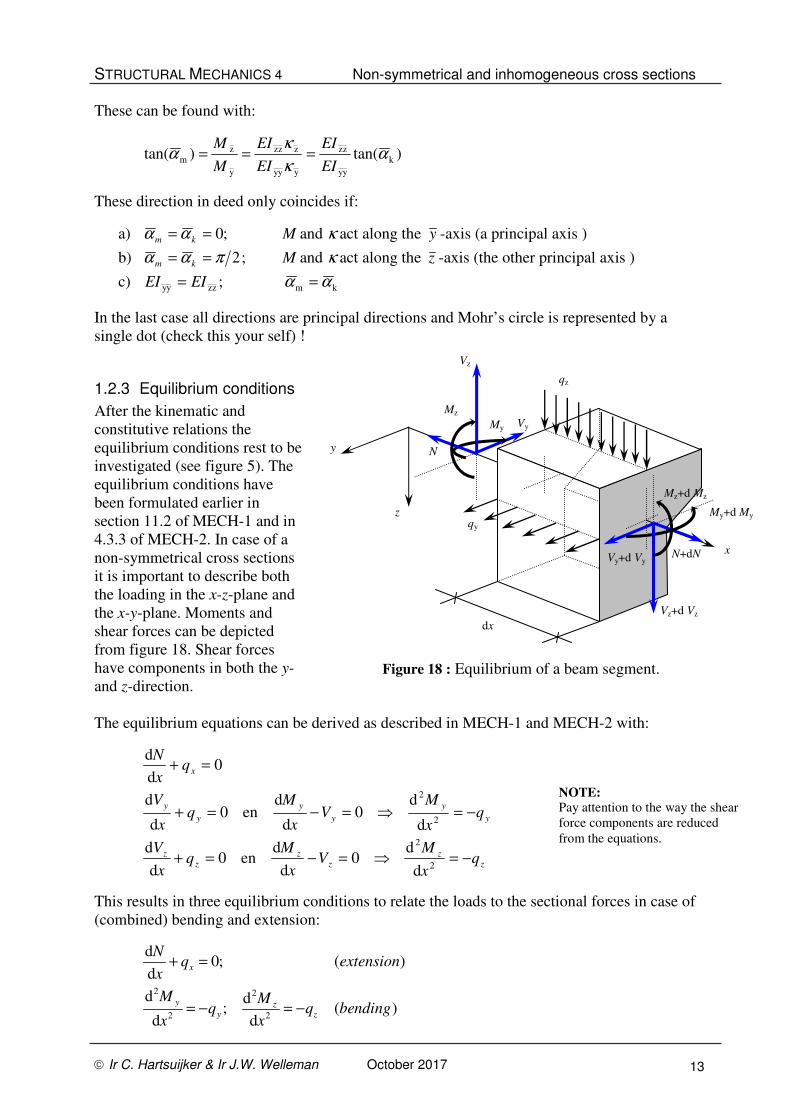
1.2.3 Equilibrium conditions
After the kinematic and
constitutive relations the
equilibrium conditions rest to be
investigated (see figure 5). The
equilibrium conditions have
been formulated earlier in
section 11.2 of MECH-1 and in
4.3.3 of MECH-2. In case of a
non-symmetrical cross sections
it is important to describe both
the loading in the x-z-plane and
the x-y-plane. Moments and
shear forces can be depicted
from figure 18. Shear forces
have components in both the y-
and z-direction.
The equilibrium equations can be derived as described in MECH-1 and MECH-2 with:
z
z
z
z
z
z
y
y
y
y
y
y
x
qx
MV
x
Mq
x
V
qx
MV
x
Mq
x
V
qx
N
−=⇒=−=+
−=⇒=−=+
=+
2
2
2
2
d
d0
d
den0
d
d
d
d0
d
den0
d
d
0d
d
This results in three equilibrium conditions to relate the loads to the sectional forces in case of
(combined) bending and extension:
2 2
2 2
d0; ( )
d
d d; ( )
d d
x
y zy z
Nq extension
x
M Mq q bending
x x
+ =
= − = −
y
z
x
Vz
Vy
Mz
My
qz
qy
N
N+dN
Vz+d Vz
Vy+d Vy
Mz+d Mz
My+d My
dx
Figure 18 : Equilibrium of a beam segment.
NOTE: Pay attention to the way the shear
force components are reduced
from the equations.

STRUCTURAL MECHANICS 4 Non-symmetrical and inhomogeneous cross sections
Ir C. Hartsuijker & Ir J.W. Welleman October 2017 14
1.2.4 Differential Equations
With the found kinematic, constitutive- and equilibrium relations it is possible to describe the
behaviour of a prismatic bar with a unsymmetrical and/or inhomogeneous cross section in the
displacements x y z, andu u u of the bar axis.
Kinematics:
d'
d
xx
uu
xε = = ;
2
2
d"
d
y
y y
uu
xκ = − = − ;
2
2
d"
d
zz z
uu
xκ = − = −
Constitutive relations:
=
z
y
zzzy
yzyy
z
y
0
0
00
κ
κ
ε
EIEI
EIEI
EA
M
M
N
Equilibrium relations:
d
dx
Nq
x= −
2
2
d
d
y
y
Mq
x= −
2
2
d
d
zz
Mq
x= −
After substitution of these relations, three differential equations occur expressed in the
displacements of the bar axis in the directions of the coordinate system:
"x xEAu q− = extension
'''' ''''
'''' ''''
yy y yz z y
yz y zz z z
EI u EI u q
EI u EI u q
+ =
+ = (double) bending
Extension is uncoupled from the two differential equations for bending. The latter two
equations for bending are coupled. However we can rewrite them as two uncoupled
equations2. Thus resulting in three ordinary differential equations to describe the behaviour of
the bar axis:
* *
2 2
* *
2
"
"'' "'' ;
"'' "'' ;
x x
yy zz y yy yz z yy zz y yy yz z
yy y yy y y y
yy zz yz yy zz yz
yz zz y yy zz z yz zz y yy zz z
zz z zz z z z
yy zz yz yy
EAu q
EI EI q EI EI q EI EI q EI EI qEI u EI u q q
EI EI EI EI EI EI
EI EI q EI EI q EI EI q EI EI qEI u EI u q q
EI EI EI EI E
= −
− −= ⇔ = =
− −
− + − += ⇔ = =
− 2
zz yzI EI−
If the boundary conditions are specified we can find the displacement field of a bar for a
certain field in the usual way. The right hand side of the second and third ODE is marked with
a *. Apart from the right hand side, these two ODE are similar to the ODE for bending in case
of symmetrical cross sections. All forget-me-nots can therefore be used if the loading is
modified according to the expression marked with the *. This will be demonstrated later in an
example.
2 Within the boundary conditions a coupling however may occur, see also APPENDIX B.
STRUCTURAL MECHANICS 4 Non-symmetrical and inhomogeneous cross sections
Ir C. Hartsuijker & Ir J.W. Welleman October 2017 15
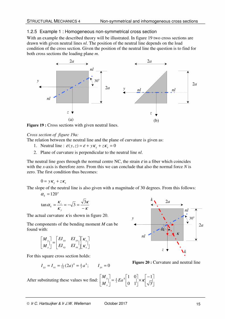
1.2.5 Example 1 : Homogeneous non-symmetrical cross section
With an example the described theory will be illustrated. In figure 19 two cross sections are
drawn with given neutral lines nl. The position of the neutral line depends on the load
condition of the cross section. Given the position of the neutral line the question is to find for
both cross sections the loading plane m.
Figure 19 : Cross sections with given neutral lines.
Cross section of figure 19a:
The relation between the neutral line and the plane of curvature is given as:
1. Neutral line : 0),( zy =++= κκεε zyzy
2. Plane of curvature is perpendicular to the neutral line nl.
The neutral line goes through the normal centre NC, the strain ε in a fiber which coincides
with the x-axis is therefore zero. From this we can conclude that also the normal force N is
zero. The first condition thus becomes:
zy0 κκ zy +=
The slope of the neutral line is also given with a magnitude of 30 degrees. From this follows:
κ
κ
κ
κα
α
−=−==
=
33tan
120
y
zk
o
k
The actual curvature κ is shown in figure 20.
The components of the bending moment M can be
found with:
=
z
y
zzzy
yzyy
z
y
κ
κ
EIEI
EIEI
M
M
For this square cross section holds:
0;)2( yz
4
344
121
zzyy ==== IaaII
After substituting these values we find:
−×
=
3
1
10
014
34
z
y κEaM
M
z
y
2a
2a
30o
(a)
z
y 2a
2a
nl
nl
nl nl
(b)
z
y
2a
30o
Figure 20 : Curvature and neutral line
nl
nl
k
k
κ αk
2a
STRUCTURAL MECHANICS 4 Non-symmetrical and inhomogeneous cross sections
Ir C. Hartsuijker & Ir J.W. Welleman October 2017 16
The position of the loading plane m can be determined with :
3)(
3tan
4
34
4
34
y
zm −=
−×
×==
κ
κα
Ea
Ea
M
M
From this result we can conclude that the plane of curvature k coincides with the loading
plane m. This is in agreement with the earlier made remarks in section 1.4.2 in which we
found that m and k coincides when the coordinate system coincides with the principal
directions of the cross section or if the cross section has equal principal values which is the
case for this cross section.
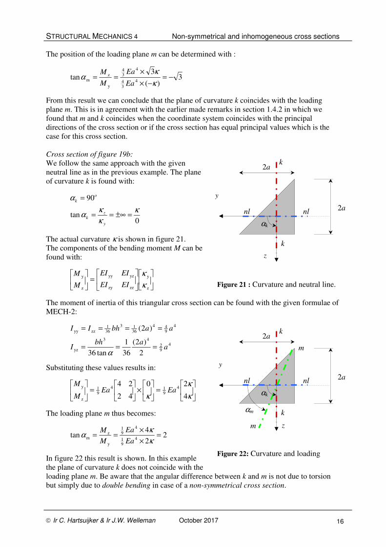
Cross section of figure 19b:
We follow the same approach with the given
neutral line as in the previous example. The plane
of curvature k is found with:
0tan
90
κ
κ
κα
α
=±∞==
=
y
zk
o
k
The actual curvature κ is shown in figure 21.
The components of the bending moment M can be
found with:
=
z
y
zzzy
yzyy
z
y
κ
κ
EIEI
EIEI
M
M
The moment of inertia of this triangular cross section can be found with the given formulae of
MECH-2:
4
92
43
yz
4
944
3613
361
zzyy
2
)2(
36
1
tan36
)2(
aabh
I
aabhII
===
====
α
Substituting these values results in:
=
×
=
κ
κ
κ 4
20
42
244
914
91
z
yEaEa
M
M
The loading plane m thus becomes:
22
4tan
4
91
4
91
y
zm =
×
×==
κ
κα
Ea
Ea
M
M
In figure 22 this result is shown. In this example
the plane of curvature k does not coincide with the
loading plane m. Be aware that the angular difference between k and m is not due to torsion
but simply due to double bending in case of a non-symmetrical cross section.
z
y
2a
2a
nl nl
k
k
αk
Figure 21 : Curvature and neutral line.
z
y
2a
2a
nl nl
k
k
αk
Figure 22: Curvature and loading
m
m
αm
STRUCTURAL MECHANICS 4 Non-symmetrical and inhomogeneous cross sections
Ir C. Hartsuijker & Ir J.W. Welleman October 2017 17
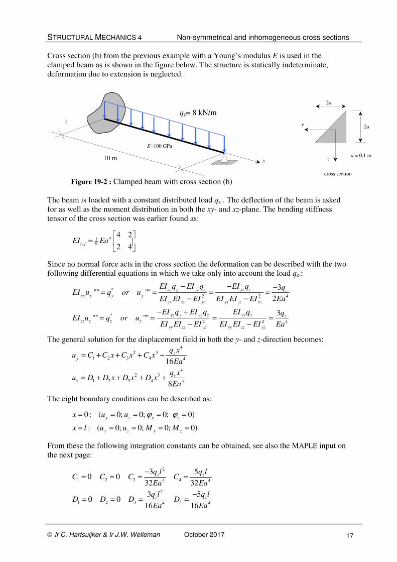
Cross section (b) from the previous example with a Young’s modulus E is used in the
clamped beam as is shown in the figure below. The structure is statically indeterminate,
deformation due to extension is neglected.
Figure 19-2 : Clamped beam with cross section (b)
The beam is loaded with a constant distributed load qz . The deflection of the beam is asked
for as well as the moment distribution in both the xy- and xz-plane. The bending stiffness
tensor of the cross section was earlier found as:
41, 9
4 2
2 4i j
EI Ea
=
Since no normal force acts in the cross section the deformation can be described with the two
following differential equations in which we take only into account the load qz.:
*
2 2 4
*
2 2 4
3"'' "''
2
3"'' "''
zz y yz z yz z zyy y y y
yy zz yz yy zz yz
yz y yy z yy z zzz z z z
yy zz yz yy zz yz
EI q EI q EI q qEI u q or u
EI EI EI EI EI EI Ea
EI q EI q EI q qEI u q or u
EI EI EI EI EI EI Ea
− − −= = = =
− −
− += = = =
− −
The general solution for the displacement field in both the y- and z-direction becomes:
42 3
1 2 3 4 4
42 3
1 2 3 4 4
16
8
zy
zz
q xu C C x C x C x
Ea
q xu D D x D x D x
Ea
= + + + −
= + + + +
The eight boundary conditions can be described as:
0 : ( 0; 0; 0; 0)
: ( 0; 0; 0; 0)
y z y z
y z y z
x u u
x l u u M M
ϕ ϕ= = = = =
= = = = =
From these the following integration constants can be obtained, see also the MAPLE input on
the next page:
2
1 2 3 44 4
2
1 2 3 44 4
3 50 0
32 32
3 50 0
16 16
z z
z z
q l q lC C C C
Ea Ea
q l q lD D D D
Ea Ea
−= = = =
−= = = =
10 m x
qz= 8 kN/m
z
y 2a
2a
cross section
E=100 GPa
a = 0,1 m
y

STRUCTURAL MECHANICS 4 Non-symmetrical and inhomogeneous cross sections
Ir C. Hartsuijker & Ir J.W. Welleman October 2017 18
The MAPLE input sheet is given below.
The moment distribution and the displacement field is shown below. Due to the load in z-
direction and the imposed boundary conditions the moment distribution in the xy-plane
becomes zero. The maximum moment at the clamped end is indeed 0,125×q×l2
= 100 kNm.
Due to the unsymmetrical cross section the member will deflect in both the xy-plane and the
xz-plane.
Figure 19-3 : Results for M and u for a cross section of type (b)
Remark:
Although the used differential equations seem to be uncoupled a coupling may exist in the
boundary conditions. In particular the dynamic boundary conditions contain a coupling:
Special care should be given to the
specified boundary conditions, see
APPENDIX B.
> restart;
> EIyy:=(4/9)*E*a^4; EIyz:=(1/2)*EIyy; EIzz:=EIyy;
> uy:=C1+C2*x+C3*x^2+C4*x^3-qz*x^4/(16*E*a^4); phiy:=-diff(uz,x): kappay:=-diff(phiz,x):
> uz:=D1+D2*x+D3*x^2+D4*x^3+qz*x^4/(8*E*a^4); phiz:=diff(uy,x): kappaz:=diff(phiy,x):
> My:=EIyy*kappay+EIyz*kappaz: Mz:=EIyz*kappay+EIzz*kappaz:
> x:=0; eq1:=uy=0; eq2:=uz=0; eq3:=phiy=0; eq4:=phiz=0;
> x:=L; eq5:=uy=0; eq6:=uz=0; eq7:=My=0; eq8:=Mz=0;
> sol:=solve({eq1,eq2,eq3,eq4,eq5,eq6,eq7,eq8},{C1,C2,C3,C4,D1,D2,D3,D4}); assign(sol);
> x:='x':
> qz:=8;L:=10; E:=100e6; a:=0.1;
> plot([-My,-Mz],x=0..L,title="Moment My and Mz",legend=["My","Mz"]);
> plot([uy,uz],x=0..L,title="Displacements uy and uz",legend=["uy","uz"]);
M
[kNm]
u
[m]
Moment My and Mz
Deflection uy and uz
'' ''; '
'' ''; '
y yy y yz z yy y yz z y y
z yz y zz z yz y zz z z z
M EI EI EI u EI u V M
M EI EI EI u EI u V M
κ κ
κ κ
= + = − − =
= + = − − =
STRUCTURAL MECHANICS 4 Non-symmetrical and inhomogeneous cross sections
Ir C. Hartsuijker & Ir J.W. Welleman October 2017 19
1.2.6 Normal stresses in the y-z-coordinate system
If for a cross section the sectional forces N, My and Mz are known, the sectional deformations
can be found with the constitutive relations:
( )
−
−
−=
=
⇒
=
=
z
y
yyzy
yzzz
2
yzzzyyz
y
z
y
zzzy
yzyy
z
y 1
M
M
EIEI
EIEI
EIEIEI
EA
N
EIEI
EIEI
M
M
EAN
κ
κ
ε
κ
κ
ε
The stress in a fiber can be found with the earlier found relation:
( )zy),(),( κκεεσ zyEzyEzy ++×=×=
In general it is of little use to elaborate this relation. For two cases however it is illustrative to
simplify the found relation.
Situation 1 : The y- and z-axis coincides with the principal axis of the cross section
If the y-z-coordinate system coincides with the principal axis of the cross section the three
sectional forces are fully uncoupled. The sectional deformation quantities can be found as:
zz
zzzzz
yy
y
yyyyy
EI
MEIM
EI
MEIM
EA
NEAN
z ==
=⇒=
==
κκ
κκ
εε
The stress distribution follows from:
( )
zz
z
yy
y
zy
),(
),(),(
I
zM
I
yM
A
Nzy
zyEzyEzy
++=
++×=×=
σ
κκεεσ
Situation 2 : The y- and z-coordinate system is thus positioned that one of the curvatures is
zero.
In this situation, one of the curvature components is zero e.g. the y-component. We then find:
y yz y z
z zz
with: 0 and
N EA
M EI
M EI
ε
κ κ κ κ
κ
=
= = =
=
The stress distribution follows from:
( )zz
z0),(),(I
zM
A
NzyEzyEzy +=+×+×=×= κεεσ
Note that the component My does not show up in the above relation for the determination of
the stress although the curvature κy is zero and the moment My is not zero!

STRUCTURAL MECHANICS 4 Non-symmetrical and inhomogeneous cross sections
Ir C. Hartsuijker & Ir J.W. Welleman October 2017 20
1.2.7 Normal stresses in the principal coordinate system
In the previous section the stresses in the cross section were found based on the defined y-z-
coordinate system. The disadvantage of this method is the coupling between the bending
components. The advantage is the straight forward method. According to the authors this
method is to be preferred. However in the engineering practice a different method is being
used. In most cases the method of the principal coordinate system is chosen. The y-z-
coordinate system is rotated to the principal zy − - coordinate system which coincides with
the principal directions of the cross section. In section 1.2.2.2 we proved that the constitutive
relations for bending are uncoupled if the principal coordinate system is used since the non
diagonal terms zyEI are zero by definition when using the principal directions as coordinate
system.
=
z
y
zz
yy
z
y
0
0
κ
κ
EI
EI
M
M
Using this approach leads in fact to the previous outlined situation 1. The formula to compute
the stress from a cross section loaded in combined bending and extension becomes:
zz
z
yy
y),(
I
zM
I
yM
A
Nzy ++=σ
The advantage of a very simple and easy to memorise formula is however small. Additional
work has to be done since all quantities used have to be referred to the rotated coordinate
system:
a) First of all the principal directions of the cross section have to be determined. We can
use Mohr’s circle or the transformation formulas for this.
b) Then the bending moment components in y- and z- direction have to be decomposed
into the principal directions.
c) In order to find the stresses in e.g. the outer fibers all the distances of this fibers have
to be transformed into the principal coordinate system.
d) All deformations and related displacements found are with respect to the principal
directions. In order to find the displacements in the original y-z coordinate system the
results have to be transformed from the principal directions back to the original
coordinate system.
To illustrate the difference between both methods an example will be shown in which both
methods are used.
NOTE: All quantities with respect to the
principal coordinate system.
STRUCTURAL MECHANICS 4 Non-symmetrical and inhomogeneous cross sections
Ir C. Hartsuijker & Ir J.W. Welleman October 2017 21
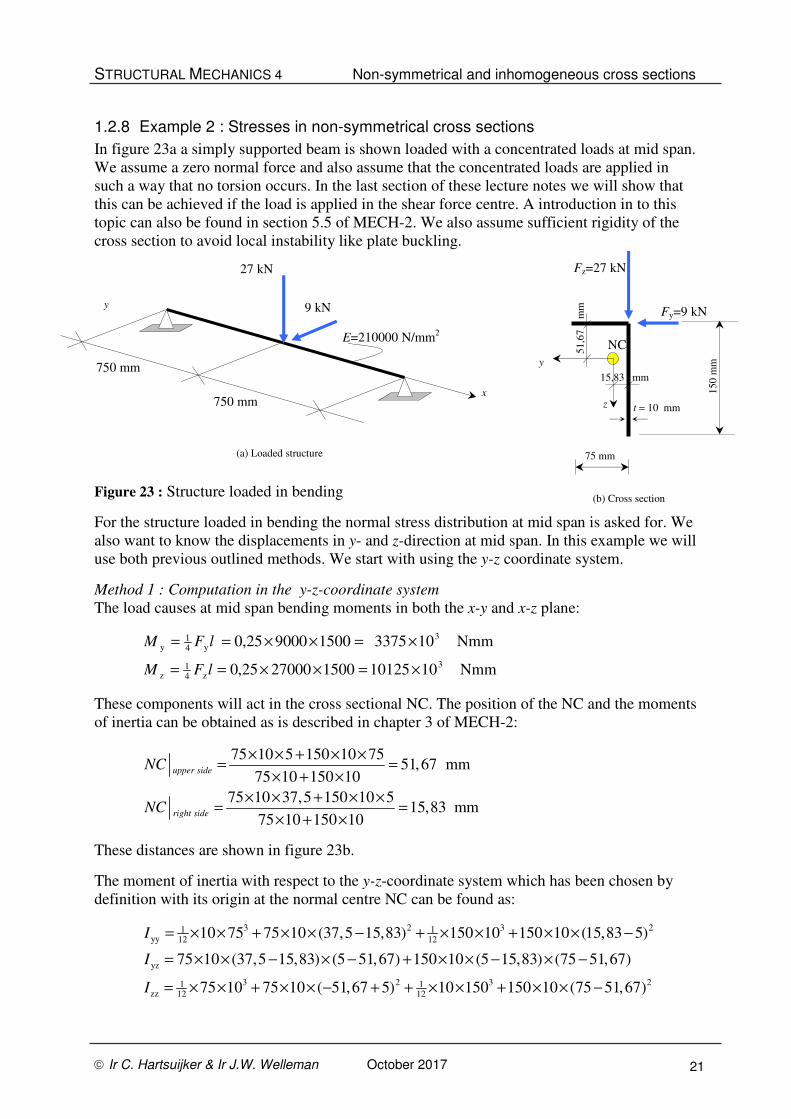
1.2.8 Example 2 : Stresses in non-symmetrical cross sections
In figure 23a a simply supported beam is shown loaded with a concentrated loads at mid span.
We assume a zero normal force and also assume that the concentrated loads are applied in
such a way that no torsion occurs. In the last section of these lecture notes we will show that
this can be achieved if the load is applied in the shear force centre. A introduction in to this
topic can also be found in section 5.5 of MECH-2. We also assume sufficient rigidity of the
cross section to avoid local instability like plate buckling.
Figure 23 : Structure loaded in bending
For the structure loaded in bending the normal stress distribution at mid span is asked for. We
also want to know the displacements in y- and z-direction at mid span. In this example we will
use both previous outlined methods. We start with using the y-z coordinate system.
Method 1 : Computation in the y-z-coordinate system
The load causes at mid span bending moments in both the x-y and x-z plane:
Nmm101012515002700025,0
Nmm1033751500900025,0
3
z41
z
3
y41
y
×=××==
×=××==
lFM
lFM
These components will act in the cross sectional NC. The position of the NC and the moments
of inertia can be obtained as is described in chapter 3 of MECH-2:
75 10 5 150 10 7551,67 mm
75 10 150 10
75 10 37,5 150 10 515,83 mm
75 10 150 10
upper side
right side
NC
NC
× × + × ×= =
× + ×
× × + × ×= =
× + ×
These distances are shown in figure 23b.
The moment of inertia with respect to the y-z-coordinate system which has been chosen by
definition with its origin at the normal centre NC can be found as:
3 2 3 21 1yy 12 12
yz
3 2 3 21 1zz 12 12
10 75 75 10 (37,5 15,83) 150 10 150 10 (15,83 5)
75 10 (37,5 15,83) (5 51,67) 150 10 (5 15,83) (75 51,67)
75 10 75 10 ( 51,67 5) 10 150 150 10 (75 51,67)
I
I
I
= × × + × × − + × × + × × −
= × × − × − + × × − × −
= × × + × × − + + × × + × × −
750 mm
750 mm
27 kN
9 kN
75 mm
150
mm
Fz=27 kN
Fy=9 kN
y
z
NC
x
15,83 mm
51,6
7
mm
(a) Loaded structure
(b) Cross section
t = 10 mm
E=210000 N/mm2
y
STRUCTURAL MECHANICS 4 Non-symmetrical and inhomogeneous cross sections
Ir C. Hartsuijker & Ir J.W. Welleman October 2017 22
From this follows:
44
zz
44
yz
44
yy mm109,526;mm1075,113;mm102,89 ×=×−=×= III
The components of the curvature in the y-z coordinate system follow from the constitutive
relation:
( )
−
−
−=
⇒
=
z
y
yyzy
yzzz
2
yzzzyyz
y
z
y
zzzy
yzyy
z
y 1
M
M
EIEI
EIEI
EIEIEIEIEI
EIEI
M
M
κ
κ
κ
κ
Using the quantities found:
( )
×
×
−−××=
−
3
3
2
4
z
y
1010125
103375
2,8975,113
75,1139,526
75,1139,5262,89
101
Eκ
κ
results in the following components of the curvature:
1/mm1099,171/mm1095,40 66 −− ×=×= zy κκ
The stress in any point of the cross section can be found with:
( )zy),(),( κκεεσ zyEzyEzy ++×=×=
Since there acts no normal force at the cross section, the stain ε in the fiber which coincides
with the x-axis (beam axis trough the NC) is also zero. This results in:
zyzy ×+×= 778,3600,8),(σ
The neutral line (points of zero strain) follows from:
0778,3600,8 =×+× zy
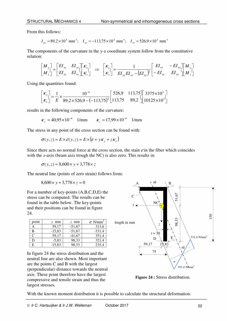
For a number of key-points (A,B,C,D,E) the
stress can be computed. The results can be
found in the table below. The key-points
and their positions can be found in figure
24.
point y mm z mm σ N/mm2
A 59,17 -51,67 313,6
B -15,83 -51,67 -331,4
C 59,17 -41,67 351,4
D -5,83 98,33 321,4
E -15,83 98,33 235,4
In figure 24 the stress distribution and the
neutral line are also shown. Most important
are the points C and B with the largest
(perpendicular) distance towards the neutral
axis. These point therefore have the largest
compressive and tensile strain and thus the
largest stresses.
With the known moment distribution it is possible to calculate the structural deformation.
75
15
0
y
z
NC
15,83
51
,67
t = 10
A B
E
59,17
98
,33
length in mm
nl
nl
C
D
+
-
351,4 N/mm2
331,4 N/mm2
Figure 24 : Stress distribution.

STRUCTURAL MECHANICS 4 Non-symmetrical and inhomogeneous cross sections
Ir C. Hartsuijker & Ir J.W. Welleman October 2017 23
Up to now we are used to calculate the displacements using the engineering forget-me-not
formulae. However in case of non-symmetrical cross sections we hit a problem using this
formulae. Several methods to obtain the displacements will be demonstrated. First the
modified forget-me-nots will be used, then the displacement based on the curvature
distribution will be used and the last option is to solve the whole problem in the principal
directions.
Displacements in the original coordinate system with modified forget-me-nots
Since the boundary conditions are fully uncoupled the modified forget-me-nots can be used.
The load in y- and z-direction are re-written as:
*
2
*
2
20461,30936 N
53087,27357 N
yy zz y yy yz z
y
yy zz yz
yz zz y yy zz z
z
yy zz yz
EI EI F EI EI FF
EI EI EI
EI EI F EI EI FF
EI EI EI
−= =
−
− += =
−
At mid span the displacements can be found using the standard forget-me-nots by using the
modified loads:
* 3
* 3
7,68 mm48
3,37 mm48
y
y
yy
zz
zz
F lu
EI
F lu
EI
= =
= =
Displacements in the original coordinate system based on the curvature distribution:
The curvature distribution is known. With the paradigma of the curvature plane the deflection
can be obtained. In the following intermezzo a brush up of this method can be found.
In figure 25 a sketch of the curvature distribution is shown. All deformation is concentrated at the bend
and denoted by theta.
Figure 25 : Basis for forget-me-not formulae
In case of a non-symmetrical cross section the reduced moment distribution Mz/EIzz is not the curvature
component κz. The correct curvature components should be obtained from the constitutive relation:
( )
−
−
−=
z
y
yyzy
yzzz
2
yzzzyyz
y 1
M
M
EIEI
EIEI
EIEIEIκ
κ
Only in case the coordinate system coincides with the principal directions of the cross section, we can
use the engineering formulae. For all other cases we should use the complete constitutive relation and
calculate the components of the curvature distribution.
Figure 26 shows the curvature distribution of the non-symmetrical beam.
F
l
zz
z
zEI
M=κ
EI
Fl−
θ
l32
θ×= lw32
EI
Fllw
EI
Fl
EI
Fll
3
23
32
2
21
=×=
=××=
θ
θ
x-axis
engineering formula

STRUCTURAL MECHANICS 4 Non-symmetrical and inhomogeneous cross sections
Ir C. Hartsuijker & Ir J.W. Welleman October 2017 24
With the paradigma of the curvature plane as described in section 8.4 in MECH-2, the
displacements in the y- en z-direction can be found.
Figure 26 : Curvature and displacements in the y-z-coordinate system.
With the boundary condition of zero displacements uy en uz at B, the rotations ϕy en ϕz at A
can be found. Subsequently the displacements at C can be found with the standard procedure:
mm37,30067,00
mm68,70154,00
61
421
)A()C()A(21
3)A(
61
221
)A()C()A(21
1)A(
=×−×−=⇒−=⇒=×−×−
=×−×−=⇒−=⇒=×−×−
llull
llull
yzyy
zyzz
θϕϕθϕ
θϕϕθϕ
Method 2: Computation in the principal coordinate system
The stresses in the key-points A to E can also be computed with the method based on the
coordinate system which coincides with the principal directions of the non-symmetrical cross
section. This method requires of course the principal directions which can be found using the
standard second order tensor formulae for the principal values and directions or by using
Mohr’s graphical method. Both ways will be illustrated .
The moments of inertia in the y-z-coordinate system were already found with method 1:
44
zz
44
yz
44
yy mm109,526;mm1075,113;mm102,89 ×=×−=×= III
Using the second order tensor transformation rules the principal moments of inertia can be
found:
( )
44
2
44
1
2
yz
2
zzyyzzyy
2,1
mm1042,61;mm1067,554
2
4
2
×=×=
+−±
+=
II
IIIIII
The principal directions can be found with:
yz o o
1,2
yy zz
2tan 2 13,73 ; 283,73
I
I Iα α= ⇔ =
−
)A(zϕ
x
l
y
θ1
1/mm1095,40 6−×=yκ
x
l
z
θ3
1/mm1099,17 6−×=zκ
A A B B
x
l21
y 1/mm1095,40 6−×=yκ
A B θ2
)A(zϕ
)A(yϕ
x
l21
z 1/mm1099,17 6−×=yκ
A B θ4
)A(yϕ
l61 l
61
STRUCTURAL MECHANICS 4 Non-symmetrical and inhomogeneous cross sections
Ir C. Hartsuijker & Ir J.W. Welleman October 2017 25
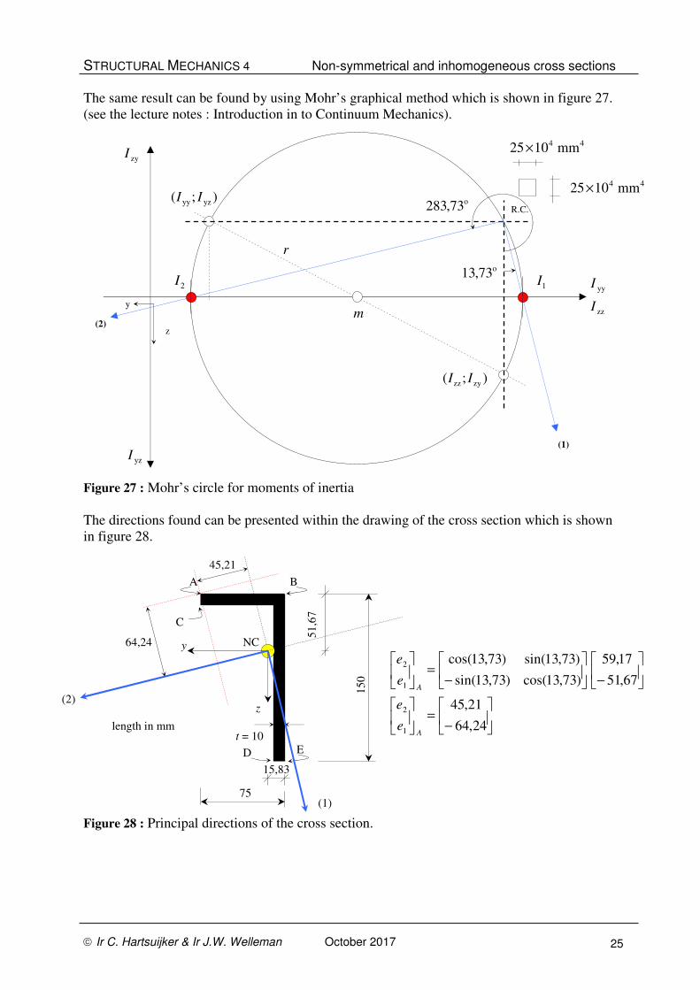
The same result can be found by using Mohr’s graphical method which is shown in figure 27.
(see the lecture notes : Introduction in to Continuum Mechanics).
Figure 27 : Mohr’s circle for moments of inertia
The directions found can be presented within the drawing of the cross section which is shown
in figure 28.
Figure 28 : Principal directions of the cross section.
zz
yy
I
I
zyI
yzI
2I 1I
44 mm1025×
44 mm1025×
m
r
);( yzyy II
);( zyzz II
z
y
R.C.
(1)
(2)
o73,13
o73,283
75
15
0
y
z
NC
15,83
51
,67
t = 10
A B
E
length in mm
(1)
C
D
(2)
64,24
45,21
−=
−
−=
24,64
21,45
67,51
17,59
)73,13cos()73,13sin(
)73,13sin()73,13cos(
1
2
1
2
A
A
e
e
e
e
STRUCTURAL MECHANICS 4 Non-symmetrical and inhomogeneous cross sections
Ir C. Hartsuijker & Ir J.W. Welleman October 2017 26
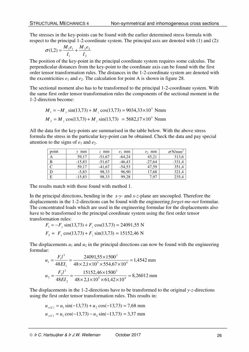
The stresses in the key-points can be found with the earlier determined stress formula with
respect to the principal 1-2-coordinate system. The principal axis are denoted with (1) and (2):
2
22
1
11)2,1(I
eM
I
eM+=σ
The position of the key-point in the principal coordinate system requires some calculus. The
perpendicular distances from the key-point to the coordinate axis can be found with the first
order tensor transformation rules. The distances in the 1-2-coordinate system are denoted with
the excentricities e1 and e2. The calculation for point A is shown in figure 28.
The sectional moment also has to be transformed to the principal 1-2-coordinate system. With
the same first order tensor transformation rules the components of the sectional moment in the
1-2-direction become:
Nmm1017,5682)73,13sin()73,13cos(
Nmm1033,9034)73,13cos()73,13sin(
3
2
3
1
×=+=
×=+−=
zy
zy
MMM
MMM
All the data for the key-points are summarised in the table below. With the above stress
formula the stress in the particular key-point can be obtained. Check the data and pay special
attention to the signs of e1 and e2.
point y mm z mm e1 mm e2 mm σ N/mm2
A 59,17 -51,67 -64,24 45,21 313,6
B -15,83 -51,67 -46,43 -27,64 -331,4
C 59,17 -41,67 -54,53 47,59 351,4
D -5,83 98,33 96,90 17,68 321,4
E -15,83 98,33 99,28 7,97 235,4
The results match with those found with method 1.
In the principal directions, bending in the x-y- and x-z-plane are uncoupled. Therefore the
displacements in the 1-2-directions can be found with the engineering forget-me-not formulae.
The concentrated loads which are used in the engineering formulae for the displacements also
have to be transformed to the principal coordinate system using the first order tensor
transformation rules:
N15152,46)73,13sin()73,13cos(
N24091,55)73,13cos()73,13sin(
2
1
=+=
=+−=
zy
zy
FFF
FFF
The displacements u1 and u2 in the principal directions can now be found with the engineering
formulae:
mm 26012,81042,61101,248
150046,15152
48
mm 4542,11067,554101,248
150055,24091
48
45
3
2
3
22
45
3
1
3
11
=××××
×==
=××××
×==
EI
lFu
EI
lFu
The displacements in the 1-2-directions have to be transformed to the original y-z-directions
using the first order tensor transformation rules. This results in:
mm37,3)73,13sin()73,13cos(
mm68,7)73,13cos()73,13sin(
21)(
21)(
=−−−=
=−+−=
uuu
uuu
Cz
Cy
STRUCTURAL MECHANICS 4 Non-symmetrical and inhomogeneous cross sections
Ir C. Hartsuijker & Ir J.W. Welleman October 2017 27
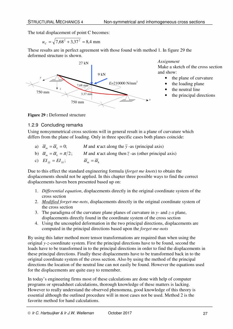
The total displacement of point C becomes:
mm4,837,368,7 22 =+=Cu
These results are in perfect agreement with those found with method 1. In figure 29 the
deformed structure is shown.
Figure 29 : Deformed structure
1.2.9 Concluding remarks
Using nonsymmetrical cross sections will in general result in a plane of curvature which
differs from the plane of loading. Only in three specific cases both planes coincide:
a) ;0== km αα M and κ act along the y -as (principal axis)
b) ;2παα == km M and κ act along then z -as (other principal axis)
c) ;zzyy EIEI = km αα =
Due to this effect the standard engineering formula (forget me knots) to obtain the
displacements should not be applied. In this chapter three possible ways to find the correct
displacements haven been presented based up on:
1. Differential equation, displacements directly in the original coordinate system of the
cross section
2. Modified forget-me-nots, displacements directly in the original coordinate system of
the cross section
3. The paradigma of the curvature plane planes of curvature in y- and z-x plane,
displacements directly found in the coordinate system of the cross section
4. Using the uncoupled deformation in the two principal directions, displacements are
computed in the principal directions based upon the forget-me-nots
By using this latter method more tensor transformations are required than when using the
original y-z-coordinate system. First the principal directions have to be found, second the
loads have to be transformed in to the principal directions in order to find the displacements in
these principal directions. Finally these displacements have to be transformed back in to the
original coordinate system of the cross section. Also by using the method of the principal
directions the location of the neutral line can not easily be found. However the equations used
for the displacements are quite easy to remember.
In today’s engineering firms most of these calculations are done with help of computer
programs or spreadsheet calculations, thorough knowledge of these matters is lacking.
However to really understand the observed phenomena, good knowledge of this theory is
essential although the outlined procedure will in most cases not be used. Method 2 is the
favorite method for hand calculations.
750 mm
750 mm
27 kN
9 kN
x
E=210000 N/mm2
7,68 mm
3,37 mm
y
z
Assignment
Make a sketch of the cross section
and show:
• the plane of curvature
• the loading plane
• the neutral line
• the principal directions
STRUCTURAL MECHANICS 4 Non-symmetrical and inhomogeneous cross sections
Ir C. Hartsuijker & Ir J.W. Welleman October 2017 28
1.3 Extension of the theory for inhomogeneous cross sections
If the cross section is not made out of one single (homogeneous) material the cross section is
considered to be an inhomogeneous cross section. In the fiber model used the inhomogeneous
character can be implemented by using a function for the Young’s modulus or modulus of
elasticity E. The modulus of elasticity may vary between fibers based on material used for
each fiber or part of the cross section. The Young’s function used is denoted as:
),( zyE
Since the Young’s modulus only appears in the constitutive relations used in the model, only
this part of the model has to be extended.
The constitutive relation which relates the stresses to the strains has to be modified slightly:
),(),(),( zyzyEzy εσ ×=
Since the kinematic relation will not change the three cross sectional deformation quantities
zy ,, κκε can still be used to describe the strain distribution of the cross section. This
strain distribution still appears to be a plane from which follows that cross sections remain
plane also after deformation.
For each fiber (y,z) of the cross section the strain can be determined with:
zy),( κκεε zyzy ++=
The stress in a specific fiber becomes in case of linear elasticity (Hooke’s law):
( )zy),(),( κκεσ zyzyEzy ++×=
The stress distribution will not be a linear distributed function. This will have consequences
for the evaluation of the integrals used to calculate the sectional forces.
The normal force N can be found with (see section 1.2.2):
( )
∫ ∫∫
∫∫
++=
⇔++×==
A AA
AA
zdAzyEydAzyEdAzyE
dAzyzyEdAzyN
),(),(),(
),(),(
zy
zy
κκε
κκεσ
The expressions for the components of the bending moment My and Mz yield:
( )
( )
∫ ∫∫
∫∫
∫ ∫∫
∫∫
++=
⇔++×==
++=
⇔++×==
A AA
AA
A AA
AA
dAzzyEyzdAzyEzdAzyE
zdAzyzyEdAzyzM
yzdAzyEdAyzyEydAzyE
ydAzyzyEdAzyyM
2
zy
zyz
z
2
y
zyy
),(),(),(
),(),(
),(),(),(
),(),(
κκε
κκεσ
κκε
κκεσ
As can be seen from these expressions, the Young’s function E(y,z) remains under the
integral.
NOTE:
We will still consider a linear elastic stress-
strain relation for each fiber.

STRUCTURAL MECHANICS 4 Non-symmetrical and inhomogeneous cross sections
Ir C. Hartsuijker & Ir J.W. Welleman October 2017 29
In order to obtain expressions which can be handled we will introduce new cross sectional
quantities which will be denoted with so-called double letter symbols:
zz
2
zyyz
yy
2
y
),(
),(),(
),(),(),(
EIdAzzyE
EIEIyzdAzyEESzdAzyE
EIdAyzyEESydAzyEEAdAzyE
A
A
z
A
AAA
=
===
===
∫
∫∫
∫∫∫
The expressions found on the previous page can now be rewritten using these double letter
symbols. The cross sectional constitutive relation which relates the sectional forces (N, My and
Mz ) to the sectional deformations (ε, κy and κz) thus becomes:
zzzyzyzz
zyzyyyyy
zzyy
κκε
κκε
κκε
EIEIESM
EIEIESM
ESESEAN
++=
++=
++=
In matrix notation this constitutive relation becomes:
=
z
y
zzzyz
yzyyy
zy
z
y
κ
κ
ε
EIEIES
EIEIES
ESESEA
M
M
N
When comparing this result with the earlier found result of section 1.2.2 we hardly observe
any difference. However the double letter symbols represent the evaluation of an (extensive)
integral where as the symbols used in section 1.2.2 are the product of two quantities e.g. EA
represents E times A. For inhomogeneous situations the double letter symbol EA represents:
∫=A
dAzyEEA ),(
If we choose the origin of the coordinate system at the normal centre (NC) of the cross section
the coupling terms between extension and bending will vanish since these become zero due to
the definition of the NC:
0),(
0),(
z
y
==
==
∫
∫
A
A
zdAzyEES
ydAzyEES
with respect to the coordinate system chosen at the NC
The constitutive relation can now be simplified to:
=
z
y
zzzy
yzyy
z
y
0
0
00
κ
κ
ε
EIEI
EIEI
EA
M
M
N
basic formula (1)
Again we observe that bending and extension are uncoupled if we choose the origin of the
coordinate system at the NC.

STRUCTURAL MECHANICS 4 Non-symmetrical and inhomogeneous cross sections
Ir C. Hartsuijker & Ir J.W. Welleman October 2017 30
In order to find the stresses in a cross section we first have to find with basic formula 1 the
cross sectional deformations. Subsequently we can find the strain of a specific fiber with:
zy),( κκεε zyzy ++= basic formula (2)
The stress in a specific fiber can be found with:
),(),(),( zyzyEzy εσ ×= basic formula (3)
This strategy is summarised in the scheme of figure 30.
Figure 30 : Calculation scheme.
Since the modulus of elasticity may vary across the cross section, the stress distribution will
not be congruous to the strain distribution. A single simplified expression for the stress can
therefore not be found for inhomogeneous situations.
- localise the NC - compute
EA, EIyy, EIzz, EIyz
- determine the cross sectional
forces N, My and Mz
- calculate the cross sectional
deformations ),,( zy κκε
- find the strain distribution
- find the stress distribution
basic formula 1
basis formula 2
basis formula 3

STRUCTURAL MECHANICS 4 Non-symmetrical and inhomogeneous cross sections
Ir C. Hartsuijker & Ir J.W. Welleman October 2017 31
1.3.1 Position of the NC for inhomogeneous cross sections
The special location of the origin of the coordinate system for which the coupling terms (ESy
and ESz ) between extension and bending become zero is by definition called the normal force
centre NC. The result of this definition is that an axial force N which acts at the NC only
causes straining and no bending. The coupling terms are also referred to as weighted static
moments or weighted first order moments. To find the position of the coordinate system for
which the coupling terms become zero requires a tool.
Figure 31 : Weighted Static Moment of the cross section.
Assume a temporary zy − -coordinate system from which the position is known and shown in
figure 31. The shift in origin of this coordinate system with respect to the y-z-coordinate
system through the unknown NC is denoted with NC
y and NCz . The temporary coordinate
system can be expressed in terms of the y-z-coordinate system as:
NCNCzzzyyy +=+=
For the weighted static moments with respect to the zy − -coordinate system holds:
NCzNC
z
NCyNCy
),(),(),(
),(),(),(
zEAESdAzyEzzdAzyEdAzzyEES
yEAESdAzyEyydAzyEdAyzyEES
AAA
AAA
×+=+×=×=
×+=+×=×=
∫∫∫
∫∫∫
By definition the weighted static moments with respect to the y-z-coordinate system are zero:
0;0 zy == ESES
From which the unknown position of the NC with respect to the known position of the zy − -
coordinate system can be found:
EA
ESz
EA
ESy
zNC
y
NC
=
=
The temporary coordinate system is usually chosen along one edge of the cross section. With
an example this tool will be illustrated.
NCz
NCy
y
z
y
z
NC
dAzyE ),(
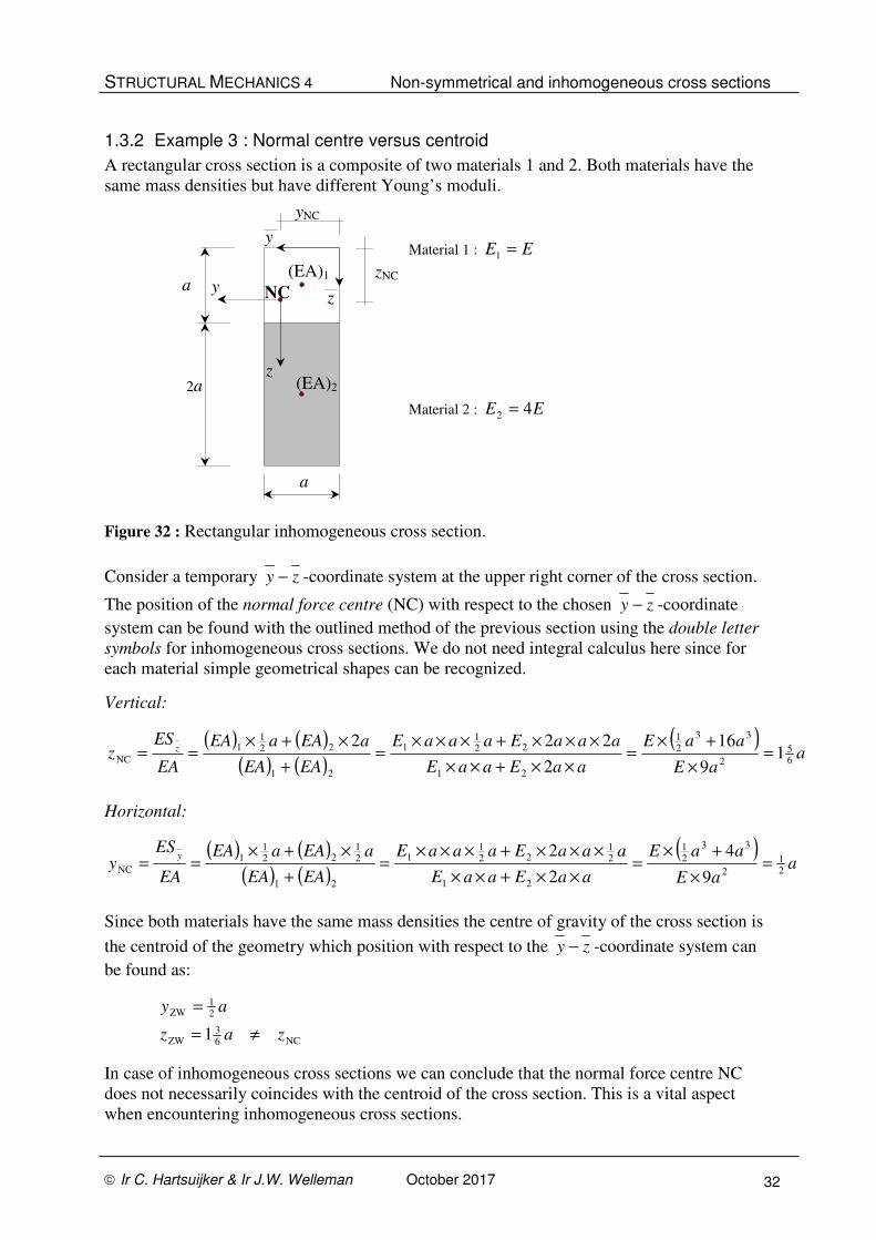
STRUCTURAL MECHANICS 4 Non-symmetrical and inhomogeneous cross sections
Ir C. Hartsuijker & Ir J.W. Welleman October 2017 32
1.3.2 Example 3 : Normal centre versus centroid
A rectangular cross section is a composite of two materials 1 and 2. Both materials have the
same mass densities but have different Young’s moduli.
Figure 32 : Rectangular inhomogeneous cross section.
Consider a temporary zy − -coordinate system at the upper right corner of the cross section.
The position of the normal force centre (NC) with respect to the chosen zy − -coordinate
system can be found with the outlined method of the previous section using the double letter
symbols for inhomogeneous cross sections. We do not need integral calculus here since for
each material simple geometrical shapes can be recognized.
Vertical:
( ) ( )( ) ( )
( )a
aE
aaE
aaEaaE
aaaEaaaE
EAEA
aEAaEA
EA
ESz z
65
2
33
21
21
221
1
21
221
1
NC 19
16
2
222=
×
+×=
××+××
×××+×××=
+
×+×==
Horizontal:
( ) ( )( ) ( )
( )a
aE
aaE
aaEaaE
aaaEaaaE
EAEA
aEAaEA
EA
ESy
y
21
2
33
21
21
21
221
1
21
21
221
1
NC9
4
2
2=
×
+×=
××+××
×××+×××=
+
×+×==
Since both materials have the same mass densities the centre of gravity of the cross section is
the centroid of the geometry which position with respect to the zy − -coordinate system can
be found as:
NC6
3ZW
21
ZW
1 zaz
ay
≠=
=
In case of inhomogeneous cross sections we can conclude that the normal force centre NC
does not necessarily coincides with the centroid of the cross section. This is a vital aspect
when encountering inhomogeneous cross sections.
a
a
2a
Material 1 : EE =1
Material 2 : EE 42 =
z
y NC
yNC
zNC
y
z
(EA)1
(EA)2
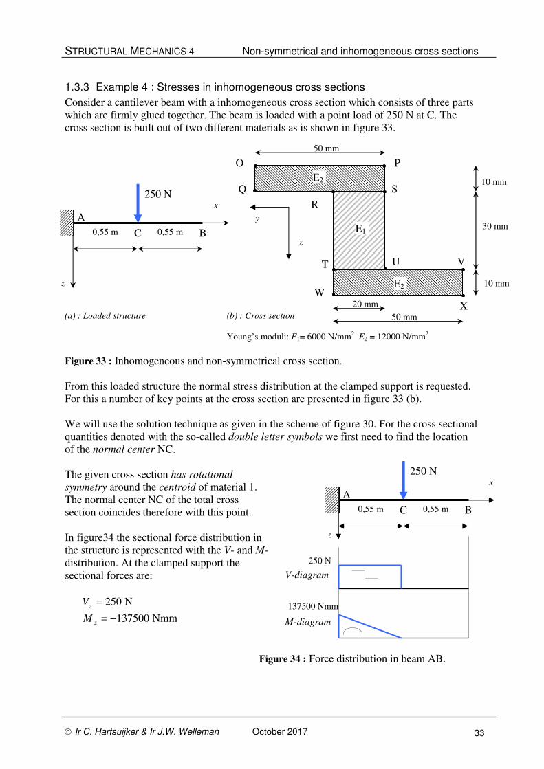
STRUCTURAL MECHANICS 4 Non-symmetrical and inhomogeneous cross sections
Ir C. Hartsuijker & Ir J.W. Welleman October 2017 33
1.3.3 Example 4 : Stresses in inhomogeneous cross sections
Consider a cantilever beam with a inhomogeneous cross section which consists of three parts
which are firmly glued together. The beam is loaded with a point load of 250 N at C. The
cross section is built out of two different materials as is shown in figure 33.
(a) : Loaded structure (b) : Cross section
Young’s moduli: E1= 6000 N/mm2 E2 = 12000 N/mm
2
Figure 33 : Inhomogeneous and non-symmetrical cross section.
From this loaded structure the normal stress distribution at the clamped support is requested.
For this a number of key points at the cross section are presented in figure 33 (b).
We will use the solution technique as given in the scheme of figure 30. For the cross sectional
quantities denoted with the so-called double letter symbols we first need to find the location
of the normal center NC.
The given cross section has rotational
symmetry around the centroid of material 1.
The normal center NC of the total cross
section coincides therefore with this point.
In figure34 the sectional force distribution in
the structure is represented with the V- and M-
distribution. At the clamped support the
sectional forces are:
Nmm137500
N250
−=
=
z
z
M
V
Figure 34 : Force distribution in beam AB.
250 N
0,55 m 0,55 m
x
z
A
B C
250 N
V-diagram
M-diagram
137500 Nmm
250 N
0,55 m 0,55 m
x
z
A
B
y
E1
E2
10 mm
30 mm
20 mm
z C
E2
10 mm
50 mm
50 mm
O P
Q S
T V
W
X
R
U
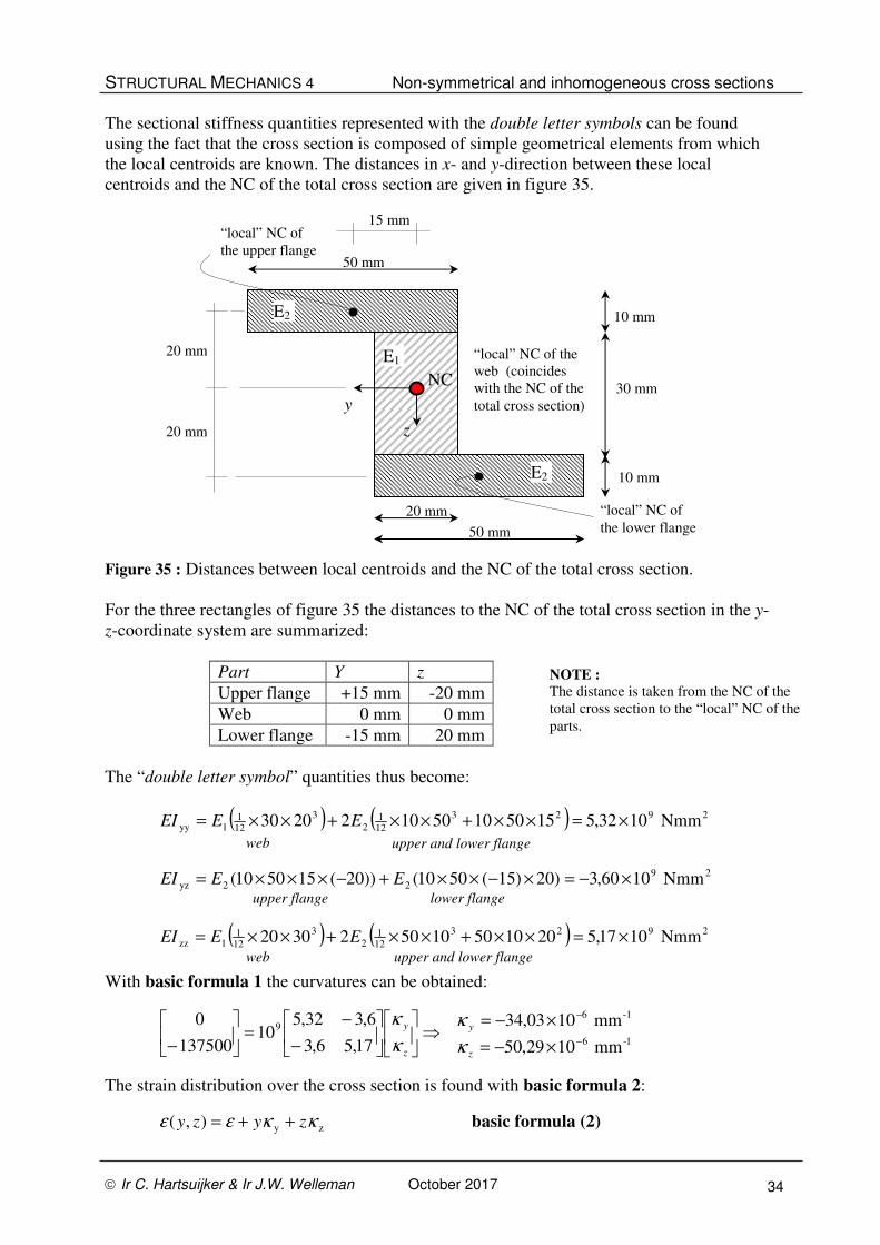
STRUCTURAL MECHANICS 4 Non-symmetrical and inhomogeneous cross sections
Ir C. Hartsuijker & Ir J.W. Welleman October 2017 34
The sectional stiffness quantities represented with the double letter symbols can be found
using the fact that the cross section is composed of simple geometrical elements from which
the local centroids are known. The distances in x- and y-direction between these local
centroids and the NC of the total cross section are given in figure 35.
Figure 35 : Distances between local centroids and the NC of the total cross section.
For the three rectangles of figure 35 the distances to the NC of the total cross section in the y-
z-coordinate system are summarized:
Part Y z
Upper flange +15 mm -20 mm
Web 0 mm 0 mm
Lower flange -15 mm 20 mm
The “double letter symbol” quantities thus become:
( ) ( )
( ) ( ) 2923
121
2
3
121
1zz
29
22yz
2923
121
2
3
121
1yy
Nmm1017,5201050105023020
Nmm1060,3)20)15(5010())20(155010(
Nmm1032,5155010501022030
×=××+××+××=
×−=×−××+−×××=
×=××+××+××=
EEEI
EEEI
EEEI
With basic formula 1 the curvatures can be obtained:
1-6
-16
9
mm1029,50
mm1003,34
17,56,3
6,332,510
137500
0−
−
×−=
×−=⇒
−
−=
−z
y
z
y
κ
κ
κ
κ
The strain distribution over the cross section is found with basic formula 2:
zy),( κκεε zyzy ++= basic formula (2)
web
yf
upper and lower flange
upper flange lower flange
upper and lower flange web
y
E1
E2
10 mm
30 mm
20 mm
z
E2
10 mm
50 mm
50 mm
20 mm
20 mm
15 mm
NC
“local” NC of
the upper flange
“local” NC of
the lower flange
“local” NC of the
web (coincides
with the NC of the
total cross section)
NOTE :
The distance is taken from the NC of the
total cross section to the “local” NC of the
parts.

STRUCTURAL MECHANICS 4 Non-symmetrical and inhomogeneous cross sections
Ir C. Hartsuijker & Ir J.W. Welleman October 2017 35
The stress at any point can be found by multiplying the strain of the considered fiber with its
Young’s moudulus:
),(),(),( zyzyEzy εσ ×= basic formula (3)
Using a spread sheet like EXCEL speeds up the calculus for each key point as can be seen
from the next table.
Units N, mm
Punt y [mm] z [mm] E-modulus [N/mm2] Strain [*10
-3] Stress [N/mm
2]
Mat
eria
l 2 O 40 -25 12000 -0,10 -1,25
P -10 -25 12000 1,60 19,17
Q 40 -15 12000 -0,61 -7,28
S -10 -15 12000 1,09 13,14
Mat
eria
l 1 R 10 -15 6000 0,41 2,48
S -10 -15 6000 1,09 6,57
T 10 15 6000 -1,09 -6,57
U -10 15 6000 -0,41 -2,48
Mat
eria
l 2 T 10 15 12000 -1,09 -13,14
V -40 15 12000 0,61 7,28
W 10 25 12000 -1,60 -19,17
X -40 25 12000 0,10 1,25
For the four points R,S,T and U two stress results are possible. Depending on the material
considered either the stress in material 1 or material 2 is found by multiplying the strain at
these points with the corresponding Young’s modulus of material 1 or material 2. The result
will be a jump in the stress distribution at these points. For point S this is shown in bold in the
table above. The stress results can also be presented graphically. To draw the stress
distribution it is important to know the position of the neutral line nl. The expression for the
neutral line becomes in this case:
029,5003,34
01029,501003,340),( 66
=−−
=×−×−⇒= −−
zy
zyzyε
Since the normal force is zero the strain at the NC is also zero. This results in a neutral line
which goes through the NC which is the origin of the coordinate system. In the graph on the
next page the neutral line is drawn, perpendicular to this line the plane of curvature k is also
shown.
As is usual, the stress distribution is drawn perpendicular to the neutral line. To avoid any
ambiguity it is advised to draw the stress distribution outside of the cross section in a separate
drawing.
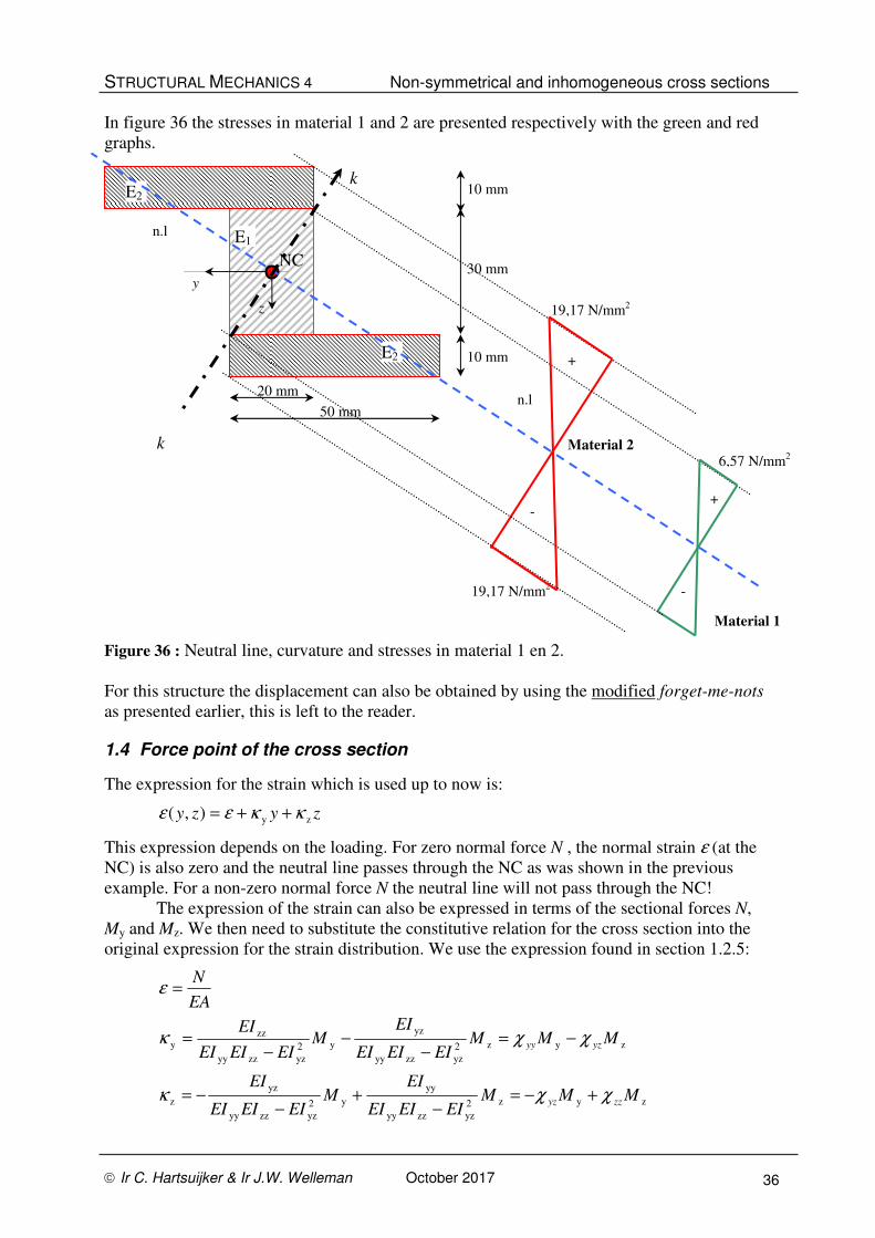
STRUCTURAL MECHANICS 4 Non-symmetrical and inhomogeneous cross sections
Ir C. Hartsuijker & Ir J.W. Welleman October 2017 36
In figure 36 the stresses in material 1 and 2 are presented respectively with the green and red
graphs.
Figure 36 : Neutral line, curvature and stresses in material 1 en 2.
For this structure the displacement can also be obtained by using the modified forget-me-nots
as presented earlier, this is left to the reader.
1.4 Force point of the cross section
The expression for the strain which is used up to now is:
zyzy zy),( κκεε ++=
This expression depends on the loading. For zero normal force N , the normal strain ε (at the
NC) is also zero and the neutral line passes through the NC as was shown in the previous
example. For a non-zero normal force N the neutral line will not pass through the NC!
The expression of the strain can also be expressed in terms of the sectional forces N,
My and Mz. We then need to substitute the constitutive relation for the cross section into the
original expression for the strain distribution. We use the expression found in section 1.2.5:
zyz2
yzzzyy
yy
y2
yzzzyy
yz
z
zyz2
yzzzyy
yz
y2
yzzzyy
zzy
MMMEIEIEI
EIM
EIEIEI
EI
MMMEIEIEI
EIM
EIEIEI
EI
EA
N
zzyz
yzyy
χχκ
χχκ
ε
+−=−
+−
−=
−=−
−−
=
=
y
E1
E2
10 mm
30 mm
20 mm
z
E2
10 mm
50 mm
NC
n.l
n.l
k
k
19,17 N/mm2
19,17 N/mm2
Material 2 6,57 N/mm
2
+
+ -
-
Material 1

STRUCTURAL MECHANICS 4 Non-symmetrical and inhomogeneous cross sections
Ir C. Hartsuijker & Ir J.W. Welleman October 2017 37
The strain distribution can thus be found with:
( ) ( ) zMMyMMEA
Nzy ×+−+×−+= zzzyyzzyzyyy),( χχχχε
If the normal force N is non-zero the moments in the xy- and yz-plane can also be expressed in
the eccentric applied normal force N:
zz
yy
eNM
eNM
×=
×=
The three sectional forces N, My and Mz are thus replaced with one single eccentric normal
force N which acts in a point at location (ey, ez) towards the NC. This point is referred to as
the force point. The expression for the strain can now be elaborated as:
( ) ( )
( ) ( )[ ]zeEAeEAyeEAeEAEA
Nzy
zeNeNyeNeNEA
Nzy
××+×−+××−×+=
⇔××+×−+××−×+=
zzzyyzzyzyyy
zzzyyzzyzyyy
1),(
),(
χχχχε
χχχχε
This last expression shows the strain ε at a point (y,z) for a normal force N acting at (ey, ez).
As an experiment of mind we can think of a force N acting in (y,z) and observing the strain ε
in (ey, ez). It appears to result in exactly the same strain. The experiment is shown in figure 36.
Figure 37 : Maxwell’s reciprocal theorem
In words we can summarise this phenomenon as:
The strain in P due to a force N in Q is equal to the strain in Q due to a force N in P.
This is also known as Maxwell’s reciprocal theorem and is general applicable to linear
elastic systems for which the superposition theorem holds. We will make use of this theorem
in the next sections.
Special case for force point:
If the yz-coordinate system coincides with the principal directions of the cross section the
expression for the strain can be simplified. In case of principal directions holds:
zz
zz
yy
yyyz
1;
1;0
EIEI=== χχχ
P
Q
P
Q
ε
ε
N
N

STRUCTURAL MECHANICS 4 Non-symmetrical and inhomogeneous cross sections
Ir C. Hartsuijker & Ir J.W. Welleman October 2017 38
The strain can be expressed as:
××+
××+=
zz
z
yy
y1),(
EI
zeEA
EI
yeEA
EA
Nzyε (symmetrical cross section)
After using the definition of the inertia radius i :
EA
EIi
EA
EIi zz2
z
yy2
y ; == (symmetrical cross section)
We can further simplify the expression for the strain:
×+
×+=
2
z
z
2
y
y1),(
i
ze
i
ye
EA
Nzyε (symmetrical cross section)
This latter result will be used in the next section on the core or kern of a cross section.
1.5 Core or Kern of a cross section
When the neutral line is inside the cross section both tensile and compressive zones will occur
on either side of the neutral line. Some materials however can hardly sustain tensile stresses
e.g. brick walls and unreinforced concrete. In case of these materials, cross sections should be
loaded in such a way that only compression occurs. The neutral line should then be outside
the cross section or just at its boundary. With this requirement the area can be determined in
which the force point should be positioned in order to prevent sign changes in the stresses.
This area is called the core or kern of the cross section.
In section 4.9 of MECH-2 the core was introduced for a
rectangular cross section with dimensions b×h as shown
in figure 38. The core appeared to be a diamond with
corner points at a distance to the NC in y- and z-
direction of respectively b61 and h
61 , see figure 38.
In this section a general method will be outlined to find
the core of inhomogeneous and or non-symmetrical
cross sections.
In the following we will make use of two important
properties which follow from the definition of the core:
o The neutral line never crosses the cross section.
o Cross sections with straight edges have a
polygon as core.
The first property follows from the requirement that the stresses in the cross section do not
change in sign. Therefore the cross section is in tension or in compression which requires a
neutral line which is outside the cross section.
y h/3
b/3
z
h
b
Figure 38 : Core of a rectangular
cross section

STRUCTURAL MECHANICS 4 Non-symmetrical and inhomogeneous cross sections
Ir C. Hartsuijker & Ir J.W. Welleman October 2017 39
As an example in figure 39 a cross section is shown. Valid positions of the neutral line are
AB, AH, HF, FE, ED and DB.
Figure 39 : Valid positions for the neutral line outside the cross section.
Based on these valid positions of the neutral line we can investigate six boundary positions of
the neutral line which will result in six force points corresponding to each position of the
neutral line, tangent to the cross sectional boundary. The force points form the core of the
cross section as will be explained in detail in an example.
The second property mentioned on the
previous page states that for cross sections
with straight edges the core also has straight
boundaries and is therefore a polygon. To
explain this we will look, as an example, to
the simple rectangular cross section given in
figure 40. From the two boundary lines 1-1
and 2-2 the according force points (core
points) are denoted as 1 and 2. The quest now
is to determine the boundary of the core
between these points 1 and 2. Force points at
the boundary of the core between 1 and 2
represent neutral lines which are tangent to the
cross section and intersect both the position of
the neutral line 1-1 and 2-2 which is at B. All
these force points between 1 and 2 will form a
straight line. We will explain this with the
Maxwell’s reciprocal theorem.
If the force point coincides with B as shown in figure 40, the neutral line can be found with
the expression for the strain in case of a symmetrical cross section, see page 38. The used
expressions for the inertia radius yield:
2
121
3
121
zz2
z
2
121
3
121
yy2
y ; hEA
Ebh
EA
EIib
EA
hEb
EA
EIi ======
With B as force point the eccentricities are:
hebe21
z21
y ; −==
A H
F G
E D
B
C
B
1 1
2
2
1
2
Figure 40 : Neutral line through corner.
z
y h
b
NOTE: A position of the neutral line which
coincide with BC can not be valid
since the neutral line then crosses
the cross section.

STRUCTURAL MECHANICS 4 Non-symmetrical and inhomogeneous cross sections
Ir C. Hartsuijker & Ir J.W. Welleman October 2017 40
The expression for the neutral line becomes:
y z
2 2
y z
1 12 2
2 21 112 12
( , ) 1 0 (neutral line)
1 0
6 61 0
e yN e zy z
EA i i
b hy z
b h
y z
b h
ε × ×
= + + = ⇔
+ × − × = ⇔
+ − =
We found in words:
For a force in B all points on a line between core point 1 and core point 2 the stresses
(and strains) are zero.
Applying Maxwell’s reciprocal theorem will result in:
For all force points on a line between core point 1 and core point 2 the stress (and
strain) at B is zero.
This proves that the boundary of the core for cross sections with straight edges is a straight
line. This also holds for non-symmetrical and or inhomogeneous cross sections since the
neutral line is a straight line. The kinematic relations will not change in case of a non-
symmetrical or inhomogeneous cross section.
If the cross section is not made out of straight edges the determination of the core becomes
quite laborious. This is shown in figure 41.
Figure 41 : Arbitrary shaped cross sections.
The core of the cross section from figure 41 (a) will consist of a polygon with four sides since
the possible positions of neutral lines which are tangent to the cross section are the four
dashed lines. For the cross section given in figure 41 (b) this no longer holds since the cross
sectional edge from A to B is curved. Every neutral line which is tangent to a point on this
edge will result in a (unique) force point which is at the boundary of the core. This results in a
curved boundary of the core between the core points 1 and 2. Core point 1 is the force points
which belongs to a neutral line which coincide with edge 1-1 and core point 2 belongs to a
neutral line which coincides with 2-2.
(a) (b)
A
B
1
1
2 2
2
1
NOTE:
For y=0 this line crosses core point 1, for z=0
the neutral line crosses core point 2.

STRUCTURAL MECHANICS 4 Non-symmetrical and inhomogeneous cross sections
Ir C. Hartsuijker & Ir J.W. Welleman October 2017 41
For arbitrary shaped cross sections we can not use the expressions given on page 38 since
these were limited to symmetrical cross sections. We therefore will use the general definition
of the neutral line as introduced in figure 11b, for cross sections with non zero normal forces:
y z
y z
( , ) 0
1 0 with: 0
y z y z
y z
ε ε κ κ
κ κε
ε ε
= + × + × = ⇔
+ × + × = ≠
To find the core points we assume a position of the
neutral line, tangent to the cross section. Suppose this
neutral line can be described with the following two
points, (y1,0) and (0,z1) as shown in figure 11c. These are
the points of intersection of the neutral line with the
coordinate axis. From the expression above we can relate
these points to the three cross sectional deformations:
z
1
y
1
κ
ε
κ
ε
−=
−=
z
y
The position of the force point which belongs to the
assumed neutral line can be found by using the cross
sectional constitutive relation:
=
=
z
y
z
y
z
y
zzzy
yzyy
z
y
:en
0
0
00
e
eN
M
M
κ
κ
ε
EIEI
EIEI
EA
M
M
N
Combining these, results in:
=
=
εκ
εκ
ε z
y
zzzy
yzyy
z
y
z
y 11
EIEI
EIEI
EAM
M
EAe
e
With the assumed position of the neutral line we now
have found the corresponding force point which is a
point at the boundary of the core:
−=
1
1
zzzy
yzyy
z
y
1
11
z
y
EIEI
EIEI
EAe
e basic formula (4)
Finding the core has reduced to a straight forward procedure in which a assumed position of
the neutral line (tangent to the cross section) is expressed by the two points of intersection
with the coordinate system from which with basic formula nr 4 the position of the core point
can be found. We will illustrate this procedure with an example.
z
y
z1
y1
n.a.
κz
κy
κ
y
z
y
z1
y1
n.l.
y ey
ez
force point
Figure 11b : Position of the neutral axis
in the cross section
Figure 11c : Position of the force point
which belongs to a neutral
axis which is tangent to the
cross section
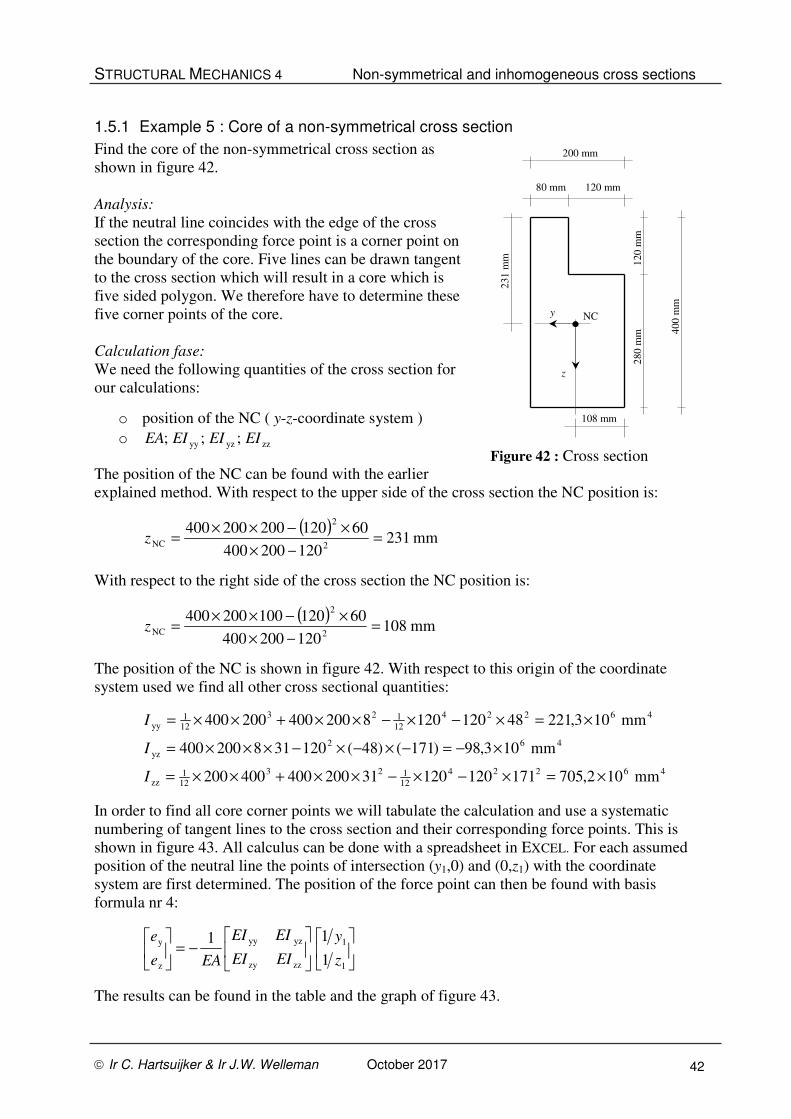
STRUCTURAL MECHANICS 4 Non-symmetrical and inhomogeneous cross sections
Ir C. Hartsuijker & Ir J.W. Welleman October 2017 42
1.5.1 Example 5 : Core of a non-symmetrical cross section
Find the core of the non-symmetrical cross section as
shown in figure 42.
Analysis:
If the neutral line coincides with the edge of the cross
section the corresponding force point is a corner point on
the boundary of the core. Five lines can be drawn tangent
to the cross section which will result in a core which is
five sided polygon. We therefore have to determine these
five corner points of the core.
Calculation fase:
We need the following quantities of the cross section for
our calculations:
o position of the NC ( y-z-coordinate system )
o zzyzyy ;;; EIEIEIEA
The position of the NC can be found with the earlier
explained method. With respect to the upper side of the cross section the NC position is:
( )
mm231120200400
601202002004002
2
NC =−×
×−××=z
With respect to the right side of the cross section the NC position is:
( )
mm108120200400
601201002004002
2
NC =−×
×−××=z
The position of the NC is shown in figure 42. With respect to this origin of the coordinate
system used we find all other cross sectional quantities:
46224
12123
121
zz
462
yz
46224
12123
121
yy
mm102,70517112012031200400400200
mm103,98)171()48(120318200400
mm103,221481201208200400200400
×=×−×−××+××=
×−=−×−×−×××=
×=×−×−××+××=
I
I
I
In order to find all core corner points we will tabulate the calculation and use a systematic
numbering of tangent lines to the cross section and their corresponding force points. This is
shown in figure 43. All calculus can be done with a spreadsheet in EXCEL. For each assumed
position of the neutral line the points of intersection (y1,0) and (0,z1) with the coordinate
system are first determined. The position of the force point can then be found with basis
formula nr 4:
−=
1
1
zzzy
yzyy
z
y
1
11
z
y
EIEI
EIEI
EAe
e
The results can be found in the table and the graph of figure 43.
80 mm 120 mm
120
mm
2
80
mm
400
mm
200 mm
108 mm
231
mm
NC y
z
Figure 42 : Cross section
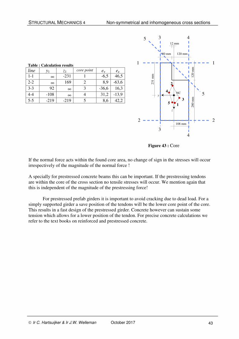
STRUCTURAL MECHANICS 4 Non-symmetrical and inhomogeneous cross sections
Ir C. Hartsuijker & Ir J.W. Welleman October 2017 43
If the normal force acts within the found core area, no change of sign in the stresses will occur
irrespectively of the magnitude of the normal force !
A specially for prestressed concrete beams this can be important. If the prestressing tendons
are within the core of the cross section no tensile stresses will occur. We mention again that
this is independent of the magnitude of the prestressing force!
For prestressed prefab girders it is important to avoid cracking due to dead load. For a
simply supported girder a save position of the tendons will be the lower core point of the core.
This results in a fast design of the prestressed girder. Concrete however can sustain some
tension which allows for a lower position of the tendon. For precise concrete calculations we
refer to the text books on reinforced and prestressed concrete.
80 mm 120 mm
120
mm
2
80
mm
108 mm
231
mm
NC y
z
Figure 43 : Core
1 1
2 2
3
3
4
4
5
5
12 mm
Table : Calculation results
line y1 z1 core point ey ez 1-1 ∞ -231 1 -6,5 46,5
2-2 ∞ 169 2 8,9 -63,6
3-3 92 ∞ 3 -36,6 16,3
4-4 -108 ∞ 4 31,2 -13,9
5-5 -219 -219 5 8,6 42,2
1
2
3
4
5
STRUCTURAL MECHANICS 4 Non-symmetrical and inhomogeneous cross sections
Ir C. Hartsuijker & Ir J.W. Welleman October 2017 44
1.6 Temperature influences*
Constrained or restricted deformations due to temperature influences may lead to considerable
stresses in structures. These stresses can even be larger than stresses due to normal loading
conditions. Temperature loads can therefore not to be neglected. In section 4.12 of MECH-2
the influence of a linear temperature gradient over the depth of a cross section is applied to a
homogeneous and symmetrical cross section. We will consider, in this section, a non
homogeneous and or unsymmetrical cross section. The temperature distribution over the
depth of the cross section can be an arbitrary function of y and z.
Using the earlier introduced constitutive relations presented with the “double letter symbols”
will be used to generalise the introduced temperature influences as introduced in MECH-2.
The modulus of elasticity E as well as the coefficient of thermal expansion α and the
temperature function T are functions depending on y and z.
),(
),(
),(
zyTT
zy
zyEE
=
=
=
αα
In the following the dependency of y and z will be omitted to simplify the expressions. The
assumptions as presented in section 1.2 will also hold in this section.
The extension of the fiber model with temperature influences results in a fiber strain which is
the combination of a strain due to stresses and a strain due to temperature influences. In order
to clearly distinct between these two components we use a upper index T or α :
Tε : strain due to temperature influences
σε : strain due to stresses
The strain in a fiber due to a temperature influence, denoted with the temperature distribution
function T(y,z) , can be expressed as:
),(),(T zyTzy αε =
The strain as a result of the stress in a fiber which results from the constitutive relation, e.g.
Hooke’s law, can be expressed as:
),(
),(),(σ
zyE
zyzy
σε =
The total strain definition thus becomes:
),(
),(),(),(),(),( σT
zyE
zyzyTzyzyzy
σαεεε +=+=
The cross sectional strain distribution can be found with the earlier derived kinematic relation:
zyzy zy),( κκεε ++=

STRUCTURAL MECHANICS 4 Non-symmetrical and inhomogeneous cross sections
Ir C. Hartsuijker & Ir J.W. Welleman October 2017 45
When we combine these latter two expressions we obtain:
{ }),(),(),( zy zyTzyzyEzy ακκεσ −++=
With this expression the cross sectional forces N, My and Mz can be determined as described
in section 1.4 using the well known “double letter symbols” :
Normal force:
{ }
dAzyTzyEESESEA
dAzyTzyzyEdAzyN
A
zzyy
AA
),(),(
),(),(),( zy
∫
∫∫
−++=
−++==
ακκε
ακκεσ
Bending moment:
dAzyTzyEzEIEIES
dAzyzM
dAzyTzyEyEIEIES
dAzyyM
A
A
A
A
),(),(
),(
),(),(
),(
zzzyzyz
z
zyzyyyy
y
∫
∫
∫
∫
−++=
=
−++=
=
ακκε
σ
ακκε
σ
With the special location of the coordinate system, chosen at the normal force center NC of
the cross section, the expressions for the sectional forces can be simplified to:
−
=
∫
∫
∫
A
A
A
AzyTzyEz
AzyTzyEy
AzyTzyE
EIEI
EIEI
EA
M
M
N
d),(),(
d),(),(
d),(),(
0
0
00
z
y
zzzy
yzyy
z
y
α
α
α
κ
κ
ε
basic formula (5)
From this expression the temperature influence becomes clear.
If a beam element is not subjected to sectional forces (unloaded) and can deform freely or
unconstrained, the deformations which may occur are only the result of a temperature
influence. The sectional deformations due to only temperature influences denoted with a
superscript T, can be found using basic formula (5):
−
=
∫
∫
∫
A
A
A
AzyTzyEz
AzyTzyEy
AzyTzyE
EIEI
EIEI
EA
d),(),(
d),(),(
d),(),(
0
0
00
0
0
0
T
z
T
y
T
zzzy
yzyy
α
α
α
κ
κ
ε
STRUCTURAL MECHANICS 4 Non-symmetrical and inhomogeneous cross sections
Ir C. Hartsuijker & Ir J.W. Welleman October 2017 46
This system of equations can be solved with the earlier derived expression for the inverse
stiffness tensor:
1
yz 2zyy yz yy zz yz
zy zzzy yy
1
0 0
0 with: detdet det
0
det det
z
EAEA
EIEIEI EI EI EI EI
EI EIEI EI
−
= − = − −
The cross sectional deformations due to temperature influences can be found as:
+−=
−=
=
∫∫
∫∫
∫
AA
AA
A
AyzTzyEzEIAyzTzyEyEI
AyzTzyEzEIAyzTzyEyEI
AzyTzyEEA
d)(),(d)(),(det
1
d)(),(d)(),(det
1
d),(),(1
yyyz
T
z
yzzz
T
y
T
αακ
αακ
αε
basic formula (6)
With this expression, basic formula (5) can be simplified to:
−
−
−
=
T
zz
T
yy
T
zzzy
yzyy
z
y
0
0
00
κκ
κκ
εε
EIEI
EIEI
EA
M
M
N
For the special case in which the coordinate system coincides with the cross sectional
principal directions, the expressions can again be simplified since the bending in the x-y and
the x-z plane are then uncoupled. The constitutive relation then becomes:
( )
( )
( ) zz
T
z
T
zzzzz
yy
T
y
T
yyyyy
TT
/d),(),(
/d),(),(
/d),(),(
EIAzyTzyEzEIM
EIAzyTzyEyEIM
EAAzyTzyEEAN
A
A
A
∫
∫
∫
=−=
=−=
=−=
ακκκ
ακκκ
αεεε
With respect to the outlined sectional method to obtain stresses and strains, only the
constitutive relations have to be modified when introducing temperature influences. However
on a structural level also some problems will arise. We will address these problems in the
forthcoming sections. To do so, it is necessary to distinct between static determinate and static
indeterminate or hyper static structures.
Static determinate structures:
If a structural element can deform unconstrained as is the case with static determinate
structures, the displacements and rotations due to the temperature influences can be
determined directly from the obtained sectional temperature deformations T
z
T
y
T en, κκε . The
temperature influence does not effect the cross sectional forces, it only results in additional
deformations which may occur freely. The sectional forces N, My and Mz are therefore only
depending upon the loading and can be found directly from the equilibrium conditions.
(only valid for the
principal coordinate
system)
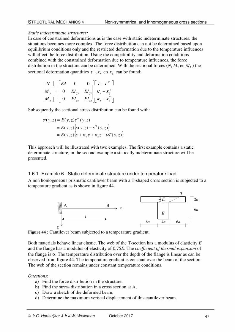
STRUCTURAL MECHANICS 4 Non-symmetrical and inhomogeneous cross sections
Ir C. Hartsuijker & Ir J.W. Welleman October 2017 47
Static indeterminate structures:
In case of constrained deformations as is the case with static indeterminate structures, the
situations becomes more complex. The force distribution can not be determined based upon
equilibrium conditions only and the restricted deformation due to the temperature influences
will effect the force distribution. Using the compatibility and deformation conditions
combined with the constrained deformation due to temperature influences, the force
distribution in the structure can be determined. With the sectional forces (N, My en Mz ) the
sectional deformation quantities zy en, κκε can be found:
−
−
−
=
T
zz
T
yy
T
zzzy
yzyy
z
y
0
0
00
κκ
κκ
εε
EIEI
EIEI
EA
M
M
N
Subsequently the sectional stress distribution can be found with:
{ }{ }),(),(
),(),(),(
),(),(),(
zy
T
zyTzyzyE
zyzyzyE
zyzyEzy
ακκε
εε
εσ σ
−++=
−=
=
This approach will be illustrated with two examples. The first example contains a static
determinate structure, in the second example a statically indeterminate structure will be
presented.
1.6.1 Example 6 : Static determinate structure under temperature load
A non homogeneous prismatic cantilever beam with a T-shaped cross section is subjected to a
temperature gradient as is shown in figure 44.
Figure 44 : Cantilever beam subjected to a temperature gradient.
Both materials behave linear elastic. The web of the T-section has a modulus of elasticity E
and the flange has a modulus of elasticity of 0,75E. The coefficient of thermal expansion of
the flange is α. The temperature distribution over the depth of the flange is linear as can be
observed from figure 44. The temperature gradient is constant over the beam of the section.
The web of the section remains under constant temperature conditions.
Questions:
a) Find the force distribution in the structure,
b) Find the stress distribution in a cross section at A,
c) Draw a sketch of the deformed beam,
d) Determine the maximum vertical displacement of this cantilever beam.
E43
E
T
6a
2a
6a 6a 4a
l
A B x
z

STRUCTURAL MECHANICS 4 Non-symmetrical and inhomogeneous cross sections
Ir C. Hartsuijker & Ir J.W. Welleman October 2017 48
Answers:
The structure is static determinate and can deform unconstrained. The force distribution can
be obtained directly from the equilibrium conditions and is independent of the temperature
load.
a) Since there is no load all sectional forces are zero.
b) To find the stress distribution we first have to find the sectional deformation quantities
due to the temperature load. We therefore need the position of the normal center and the
stiffness quantities denoted with the “double letter symbols”.
Temperature function:
The temperature function for the flange can be expressed as::
12
( , ) (1 ) with : 3z
T y z T a z aa
= − + − ≤ ≤ −
Normal center NC:
The location of the normal center NC must be on
the vertical axis of symmetry. Therefore only the
vertical position of the NC has to be found:
aaaEaaE
aaEaaaEa
EA
EAaEAaz
lijfflens
346162
)46(5)162(
)(5)(
43
43
NC
=××+××
×××+×××=
⇔×+×
=
Since this cross section has an axe of symmetry
which coincides with one of the axes of the
coordinate system, the coordinate system
coincides with the principal axis of the cross section. The coordinate system and the
location of the NC is shown in figure 45.
Axial stiffness:
The axial stiffness of the cross section can be found as:
2
43 4846162)()( EaaaEaaEEAEAEA lijfflens =××+××=+=
Bending stiffness:
Fibers at a distance z of the NC will all elongate with the same amount over the beam of
the cross section. This is of course an assumption which is reasonable for a acceptable
width of the flange. Due to symmetry the beam will not curve in the x-y-plane, 0T
y =κ .
Over the depth of the beam the fibers will elongate different. Therefore the beam will
curve in the x-z-plane. Thus we only need to determine the flexural stiffness EIzz :
{ }
{ } 423
121
23
121
43
zz
272)2(64)6(4
)2(216)2(16
EaaaaaaE
aaaaaEEI
=××+×××
+××+×××=
With basic formula (6) we can now find the sectional deformation quantities:
Figure 45 : NC of the section

STRUCTURAL MECHANICS 4 Non-symmetrical and inhomogeneous cross sections
Ir C. Hartsuijker & Ir J.W. Welleman October 2017 49
a
TEIadz
a
zTEz
TEAadza
zTE
a
a
a
a
αακ
κ
ααε
687
zz
3
21
43T
z
T
y
41
3
21
43T
/16)1(
0
/16)1(
−=×
+−×××=
=
=×
+−××=
∫
∫
−
−
−
−
The strain distribution for the cross section can be expressed as:
zzy T
z
T),( κεε +=
And the stress distribution due to the straining becomes:
{ }{ }
{ }),(),(
),(),(),(
),(),(),(
),(),(),(
T
z
T
T
σ
zyTzzyE
zyTzyzyE
zyzyzyE
zyzyEzy
ακε
αε
εε
εσ
−+×=
−×=
−×=
=×=
If we elaborate this expression for the flange we find:
+=
++×−×=
a
zTE
a
zT
a
zTTEzy
27281
272153
21
687
41
43 1),( αααασ
The expression for the web of the cross section yields:
−=
×−×=a
zTE
a
zTTEzy
27228
27268
687
41),( ααασ
The total strain and stress distribution for the cross section is shown in figure 46.
Figure 46 : Strain and stress distribution over the beams depth.
values values
fla
nge
w
eb
z TEασ ×
flens -3a -90/272
flens -a 72/272
lijf -a 96/272
lijf +5a -72/272
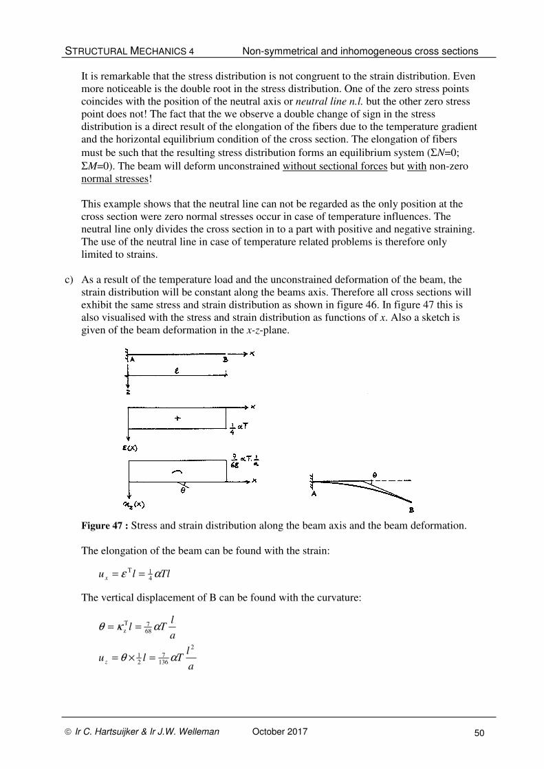
STRUCTURAL MECHANICS 4 Non-symmetrical and inhomogeneous cross sections
Ir C. Hartsuijker & Ir J.W. Welleman October 2017 50
It is remarkable that the stress distribution is not congruent to the strain distribution. Even
more noticeable is the double root in the stress distribution. One of the zero stress points
coincides with the position of the neutral axis or neutral line n.l. but the other zero stress
point does not! The fact that the we observe a double change of sign in the stress
distribution is a direct result of the elongation of the fibers due to the temperature gradient
and the horizontal equilibrium condition of the cross section. The elongation of fibers
must be such that the resulting stress distribution forms an equilibrium system (ΣN=0;
ΣM=0). The beam will deform unconstrained without sectional forces but with non-zero
normal stresses!
This example shows that the neutral line can not be regarded as the only position at the
cross section were zero normal stresses occur in case of temperature influences. The
neutral line only divides the cross section in to a part with positive and negative straining.
The use of the neutral line in case of temperature related problems is therefore only
limited to strains.
c) As a result of the temperature load and the unconstrained deformation of the beam, the
strain distribution will be constant along the beams axis. Therefore all cross sections will
exhibit the same stress and strain distribution as shown in figure 46. In figure 47 this is
also visualised with the stress and strain distribution as functions of x. Also a sketch is
given of the beam deformation in the x-z-plane.
Figure 47 : Stress and strain distribution along the beam axis and the beam deformation.
The elongation of the beam can be found with the strain:
Tllu x αε41T ==
The vertical displacement of B can be found with the curvature:
a
lTlu
a
lTl
z
2
1367
21
687T
z
αθ
ακθ
=×=
==

STRUCTURAL MECHANICS 4 Non-symmetrical and inhomogeneous cross sections
Ir C. Hartsuijker & Ir J.W. Welleman October 2017 51
1.6.2 Example 7 : Static indeterminate structure under temperature load
The same cross section will be used in a static indeterminate structure. The temperature load
is also the same as in the previous example. Both the structure and the loaded cross section
are shown in the figure below.
Figure 48 : Fully clamped beam with temperature load.
The structure is clamped at A and roller supported at B.
Questions:
a) Find the force distribution in the structure,
b) Find the stress distribution in a cross section at A,
c) Draw a sketch of the deformed beam,
d) Determine the maximum vertical displacement of this clamped beam.
Answers:
The structure is a static indeterminate structure. The deformation due to the temperature load
is therefore constrained. To find the force distribution we also have to take the deformation
behaviour into account. Applying the force method, we first choose a so called Basic Static
(determinate) System and denote one of the reaction forces as the unknown static
indeterminate since the structure is static indeterminate to the first degree. We then formulate
the deformation or compatibility condition for the associated degree of freedom of the
unknown static indeterminate. See for this method MECH-3. Since we are dealing with a
temperature load we also have to take in to account the effect of the temperature load on the
deformation.
a) As Basic Static System we choose the cantilever
structure as shown in figure 49. The unknown
static indeterminate is the vertical support
reaction at B. The associated deformation
condition becomes:
0)B(z =u
The result of the previous example can be used here since the unrestricted deformation of
the cantilever beam subjected to a temperature load was already solved. The vertical
support reaction at B becomes thus:
l
aTEB
EI
lB
a
lTu
3
V
zz
3
V
2
1367
z 4203
)B( αα =⇒=−=
The moment and shear distribution can be found using the equilibrium conditions. The
result is shown in figure 50.
l
A B x
z BV
Figure 49 : Basic Static System
E43
E
T
6a
2a
6a 6a 4a
l
A B x
z
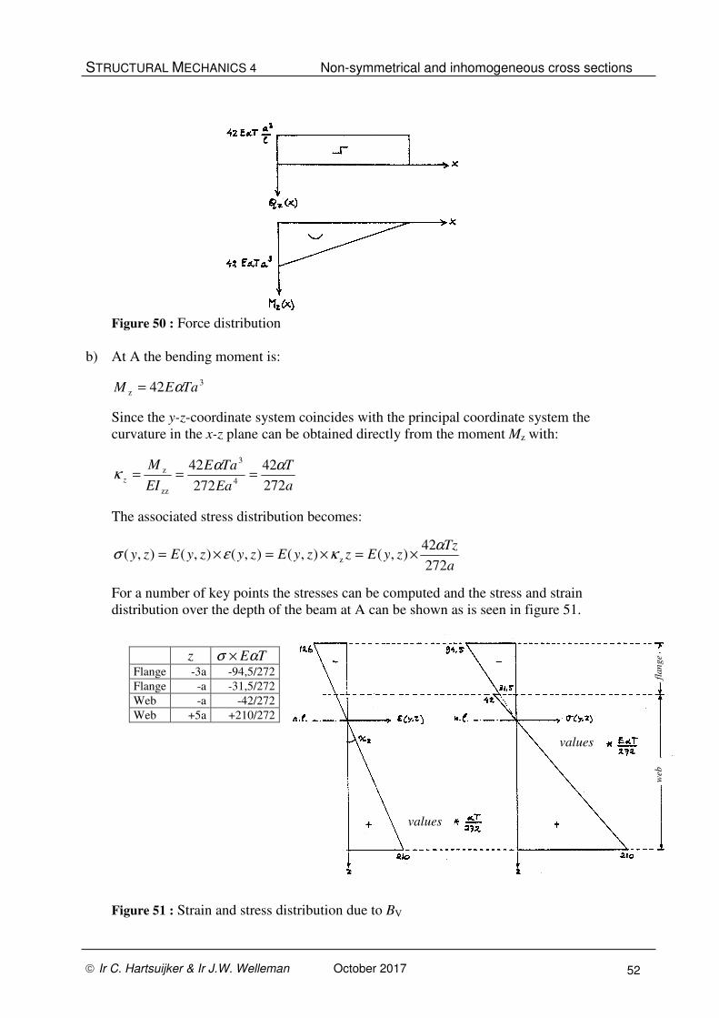
STRUCTURAL MECHANICS 4 Non-symmetrical and inhomogeneous cross sections
Ir C. Hartsuijker & Ir J.W. Welleman October 2017 52
Figure 50 : Force distribution
b) At A the bending moment is:
3
z 42 TaEM α=
Since the y-z-coordinate system coincides with the principal coordinate system the
curvature in the x-z plane can be obtained directly from the moment Mz with:
a
T
Ea
TaE
EI
Mz
272
42
272
424
3
zz
z αακ ===
The associated stress distribution becomes:
a
TzzyEzzyEzyzyEzy
272
42),(),(),(),(),( z
ακεσ ×=×=×=
For a number of key points the stresses can be computed and the stress and strain
distribution over the depth of the beam at A can be shown as is seen in figure 51.
Figure 51 : Strain and stress distribution due to BV
z TEασ × Flange -3a -94,5/272
Flange -a -31,5/272
Web -a -42/272
Web +5a +210/272
values
values
fla
nge
web

STRUCTURAL MECHANICS 4 Non-symmetrical and inhomogeneous cross sections
Ir C. Hartsuijker & Ir J.W. Welleman October 2017 53
The total strain and stress distribution can be found by superposition. The actual
distribution is the sum of distribution found in figure 51 and the distribution due to the
free or unrestricted deformation as found in the previous example. The result is shown in
figure 52.
Figure 52 : Total strain and stress distribution at A.
c) The curvature is also a summation of the earlier found curvature of the unconstrained
deformation due to the temperature load and the curvature due to the bending moment
distribution.
Figure 53 : Total curvature and deformed beam.
The displacements can be found based on the total curvature. The maximum vertical
displacement will occur at a location were the rotation ϕ is zero. From the curvature
diagram of the figure above we can observe that at C the rotation will be zero as can also
be seen from the following expression for the rotation:
values
values
fla
nge
web
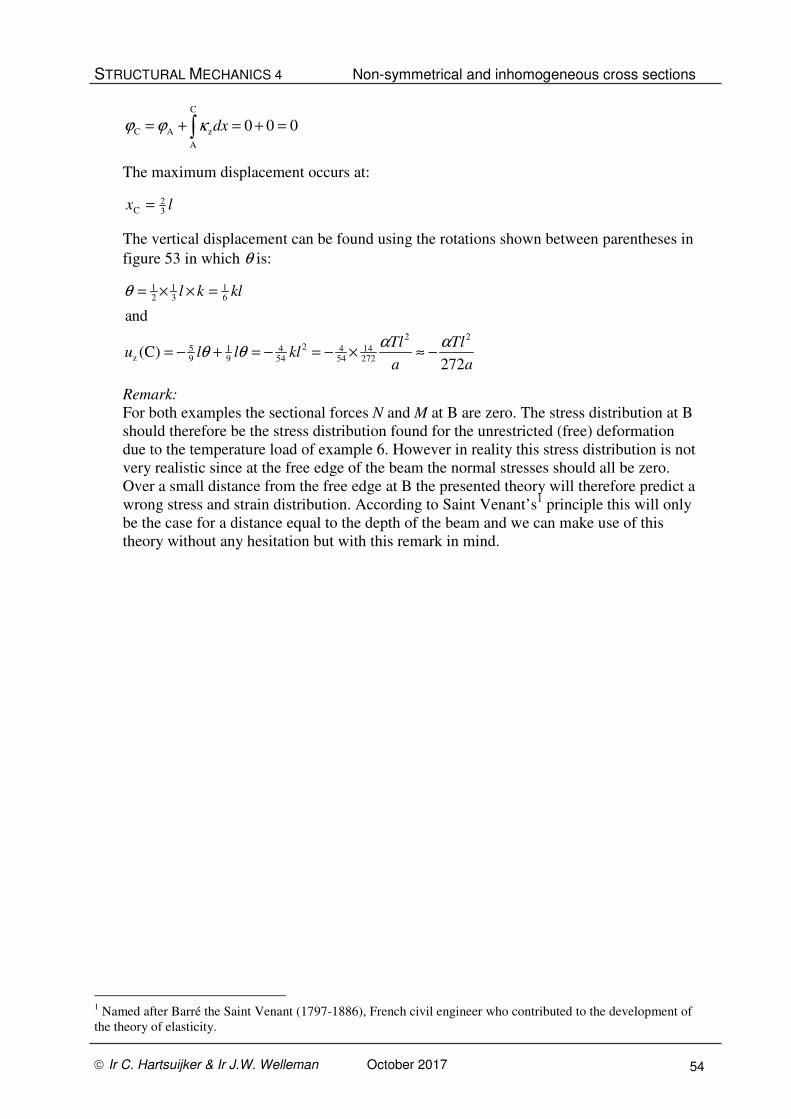
STRUCTURAL MECHANICS 4 Non-symmetrical and inhomogeneous cross sections
Ir C. Hartsuijker & Ir J.W. Welleman October 2017 54
C
C A z
A
0 0 0dxϕ ϕ κ= + = + =∫
The maximum displacement occurs at:
lx32
C =
The vertical displacement can be found using the rotations shown between parentheses in
figure 53 in which θ is:
1 1 12 3 6
2 225 1 4 4 14
z 9 9 54 54 272
and
(C)272
l k kl
Tl Tlu l l kl
a a
θ
α αθ θ
= × × =
= − + = − = − × ≈ −
Remark:
For both examples the sectional forces N and M at B are zero. The stress distribution at B
should therefore be the stress distribution found for the unrestricted (free) deformation
due to the temperature load of example 6. However in reality this stress distribution is not
very realistic since at the free edge of the beam the normal stresses should all be zero.
Over a small distance from the free edge at B the presented theory will therefore predict a
wrong stress and strain distribution. According to Saint Venant’s1 principle this will only
be the case for a distance equal to the depth of the beam and we can make use of this
theory without any hesitation but with this remark in mind.
1 Named after Barré the Saint Venant (1797-1886), French civil engineer who contributed to the development of
the theory of elasticity.
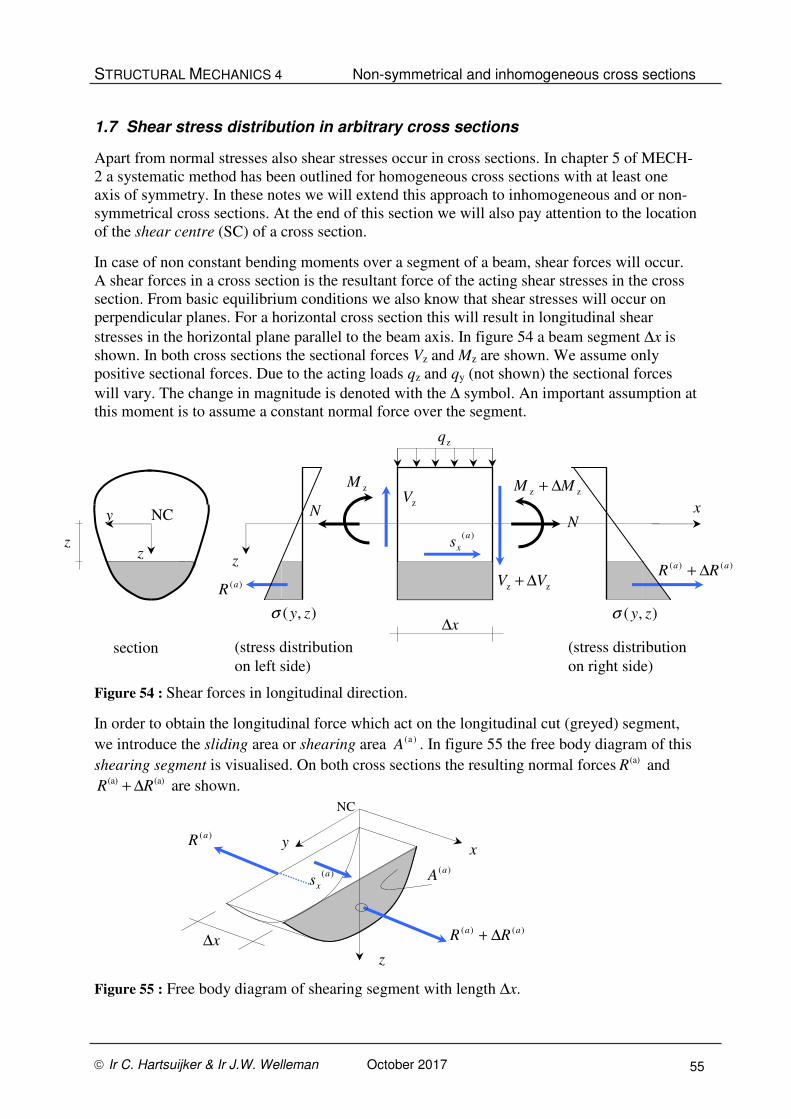
STRUCTURAL MECHANICS 4 Non-symmetrical and inhomogeneous cross sections
Ir C. Hartsuijker & Ir J.W. Welleman October 2017 55
1.7 Shear stress distribution in arbitrary cross sections
Apart from normal stresses also shear stresses occur in cross sections. In chapter 5 of MECH-
2 a systematic method has been outlined for homogeneous cross sections with at least one
axis of symmetry. In these notes we will extend this approach to inhomogeneous and or non-
symmetrical cross sections. At the end of this section we will also pay attention to the location
of the shear centre (SC) of a cross section.
In case of non constant bending moments over a segment of a beam, shear forces will occur.
A shear forces in a cross section is the resultant force of the acting shear stresses in the cross
section. From basic equilibrium conditions we also know that shear stresses will occur on
perpendicular planes. For a horizontal cross section this will result in longitudinal shear
stresses in the horizontal plane parallel to the beam axis. In figure 54 a beam segment ∆x is
shown. In both cross sections the sectional forces Vz and Mz are shown. We assume only
positive sectional forces. Due to the acting loads qz and qy (not shown) the sectional forces
will vary. The change in magnitude is denoted with the ∆ symbol. An important assumption at
this moment is to assume a constant normal force over the segment.
Figure 54 : Shear forces in longitudinal direction.
In order to obtain the longitudinal force which act on the longitudinal cut (greyed) segment,
we introduce the sliding area or shearing area )a(A . In figure 55 the free body diagram of this
shearing segment is visualised. On both cross sections the resulting normal forces (a)R and (a) (a)R R+ ∆ are shown.
Figure 55 : Free body diagram of shearing segment with length ∆x.
x∆
)(aR
)()( aa RR ∆+
)(a
xs
x
z
y
)(aA
NC
y
z z
x
z
)(aR
),( zyσ ),( zyσ
)()( aa RR ∆+
x∆
NC
section (stress distribution
on left side)
(stress distribution
on right side)
zq
zMzz MM ∆+
zz VV ∆+
NN
zV
)(a
xs

STRUCTURAL MECHANICS 4 Non-symmetrical and inhomogeneous cross sections
Ir C. Hartsuijker & Ir J.W. Welleman October 2017 56
Let us assume a shear flow (a)
xs acting on the longitudinal cut in the longitudinal direction as
shown in figure 55. This shear flow is a force per unit length. From the horizontal
equilibrium of the shearing segment with length ∆x we find the following expression for the
shear flow:
x
Rs
RRxsR
∆
∆−=
=∆++∆×+−(a)
(a)
x
(a)(a)(a)
x
(a) 0
Taking the limit for 0→∆x , the shear flow or shear force per unit of length becomes:
x
Rs
d
d (a)(a)
x −= (1)
The resulting normal force (a)R on the shearing segment follows directly from the normal
stress distribution on the shearing area )a(A :
∫=)(
d),((a)
aA
AzyR σ (2)
The normal stress distribution follows from the earlier found expression:
{ }zyzyEzy zy),(),( κκεσ ++×= (3)
The sectional deformation quantities zy en, κκε follow from the cross sectional constitutive
relation as introduced in the previous sections. We will illustrate this approach with a simple
example for which the coordinate system coincides with the principal coordinate system of
the cross section. For general situations we will derive an alternative method later.
1.7.1 Shear stress equations for principal coordinate systems
If the cross sectional y-z-coordinate system coincides with the principal coordinate system we
can use the following uncoupled constitutive relations:
zz
zz
yy
y
y
EI
M
EI
M
EA
N
=
=
=
κ
κ
ε
(4)
After combining expression (3) with expression (4) we find:
×+
×+×=
zz
z
yy
y),(),(
EI
zM
EI
yM
EA
NzyEzyσ (5)
If we substitute this result in (2) and use this in (1) we find:
∫ ∫
++×−=−=−=
)( )(
ddx
d
d
d
d
d1),(d
d
),(d
d
d z
zz
y
yy
(a)(a)
xa a
A A
AM
EI
z
x
M
EI
y
x
N
EAzyEA
x
zy
x
Rs
σ

STRUCTURAL MECHANICS 4 Non-symmetrical and inhomogeneous cross sections
Ir C. Hartsuijker & Ir J.W. Welleman October 2017 57
With the welle known expressions for the shear force we can simplify this equation:
x
MV
x
MV
y
d
d
d
d
zz
y
=
=
Since we assumed a constant normal force for the beam segment we can assume:
0d
d=
x
N
For prismatic beams the stiffness quantities denoted with the “double letter symbols”
yy zz, andEA EI EI are constant and can be put in font of the integrals. The result of all this
work is a closed formulation for the shear flow per unit of length:
×+×−= ∫∫
)()(
d),(d),(zz
z
yy
y(a)
xaa
AA
AzzyEEI
VAyzyE
EI
Vs
With the ”double letter symbols” we can simplify this to a neat basic formula:
zz
(a)
zz
yy
(a)
yy(a)
xEI
ESV
EI
ESVs −−= basic formula (7)
This expression is almost identical to the expression found in MECH-2. New element here is
the extension to two directions, y and z.
From the shear flow the shear stress can be found by dividing the shear flow with the actual
width of the longitudinal cut of the shearing segment. This is shown in figure 56 while using
the in MECH-2 introduced local m-axis for an unambiguous definition of the shear stress.
Figure 56 : Shear stresses in a beam at distance z from the NC.
The shear stresses in the cross section are the same as those in the longitudinal cut of the
shearing segment, see for the proof section 5.3.1 of MECH-2:
mxxm σσ =
mxσ
(a)
(a)
xmx
b
s=σ
Remark:
We assume a constant shear stress
over the width (a)b of a section. In
reality this is not the case. However
for engineering purposes (relative slim
cross sections) this is acceptable.
x∆
)(a
xs
x
z
y
)(aA
NC
xmσ
m-as
(a)b
z
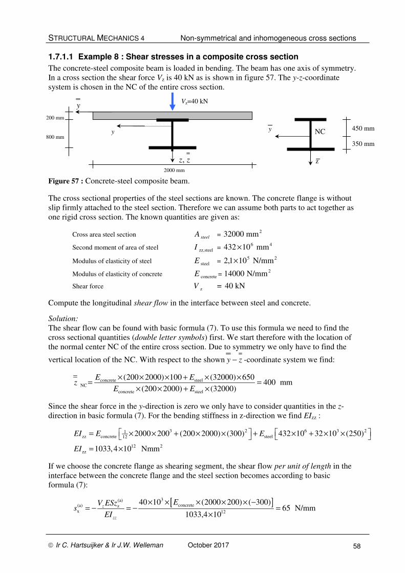
STRUCTURAL MECHANICS 4 Non-symmetrical and inhomogeneous cross sections
Ir C. Hartsuijker & Ir J.W. Welleman October 2017 58
1.7.1.1 Example 8 : Shear stresses in a composite cross section
The concrete-steel composite beam is loaded in bending. The beam has one axis of symmetry.
In a cross section the shear force Vz is 40 kN as is shown in figure 57. The y-z-coordinate
system is chosen in the NC of the entire cross section.
Figure 57 : Concrete-steel composite beam.
The cross sectional properties of the steel sections are known. The concrete flange is without
slip firmly attached to the steel section. Therefore we can assume both parts to act together as
one rigid cross section. The known quantities are given as:
Cross area steel section steelA = 2mm32000
Second moment of area of steel zz,steelI = 46 mm10432 ×
Modulus of elasticity of steel steelE = 25 N/mm101,2 ×
Modulus of elasticity of concrete concreteE = 2N/mm14000
Shear force zV = kN40
Compute the longitudinal shear flow in the interface between steel and concrete.
Solution:
The shear flow can be found with basic formula (7). To use this formula we need to find the
cross sectional quantities (double letter symbols) first. We start therefore with the location of
the normal center NC of the entire cross section. Due to symmetry we only have to find the
vertical location of the NC. With respect to the shown zy − -coordinate system we find:
concrete steelNC
concrete steel
(200 2000) 100 (32000) 650400 mm
(200 2000) (32000)
E Ez
E E
× × × + × ×= =
× × + ×
Since the shear force in the y-direction is zero we only have to consider quantities in the z-
direction in basic formula (7). For the bending stiffness in z-direction we find EIzz :
3 2 6 3 21zz concrete steel12
12 2
zz
2000 200 (200 2000) (300) 432 10 32 10 (250)
1033,4 10 Nmm
EI E E
EI
= × × + × × + × + × ×
= ×
If we choose the concrete flange as shearing segment, the shear flow per unit of length in the
interface between the concrete flange and the steel section becomes according to basic
formula (7):
[ ]3(a)
concrete(a) zx 12
40 10 (2000 200) ( 300)65 N/mm
1033,4 10
z
zz
EV ESzs
EI
× × × × × −= − = − =
×
y
zz,
200 mm
800 mm NC
-350 mm
450 mm
2000 mm
Vz=40 kN
y y
z

STRUCTURAL MECHANICS 4 Non-symmetrical and inhomogeneous cross sections
Ir C. Hartsuijker & Ir J.W. Welleman October 2017 59
1.7.2 General shear stress formula
If the principal coordinate system of the cross section does not coincide with the chosen y-z-
coordinate system we can not use the basic formula (7) since this formula was based on the
uncoupled bending terms of the constitutive relation which is only valid in the principal
coordinate system. For an arbitrary cross section with its y-z-coordinate system chosen
through the NC of the cross section we will derive a general shear stress formula. We start
with the result of the horizontal equilibrium of the shearing segment as shown in figure 54.
The shear flow per unit of length according to equation (1) is:
x
Rs
d
d (a)(a)
x −= (1)
The normal stress distribution on the shearing area A(a)
is linear and is the result of a
component due to the normal force N and a component due to the resulting moment M in the
cross section. The resultant of these stresses R(a)
can therefore also be split in to a component (a)
NR due to N and a component (a)
MR due to M:
McNcRRR 21
(a)
M
(a)
N
(a) +=+= with: 2
z
2
y MMM +=
Check for yourself that the constants c1 and c2 can be found as:
( ) ( )
1 2;a a
N MR Rc c
N M= =
Differentiating R(a)
and applying the chain rule we find for the shear flow (1):
VM
R
x
M
M
Rs
aaa
xd
d
d
d
d
d )()()( −=−= with: 2
z
2
y VVV +=
In this expression V is the resulting shear force in the cross section. Substituting the linear
relation for R(a)
with respect to N and M we can rewrite this expression as:
(a)
(a) 1 2 Mx 2
d( )
d
c N c M Rs V V c V
M M
+= − = − = − basic formula (8)
In words this formula says that the shear flow per unit of length is equal to the resultant shear
force V multiplied with a scaling factor. This scaling factor is the resultant of the normal
stresses on the shearing segment due to bending only divided by the resultant moment M in
the cross section.
Note that the scaling factor is independent of the magnitude of M. Important in the
application of this method is however that both the shear force V and the moment M
act in the same loading plane since we made use of the equilibrium condition:
x
MV
d
d=
If in a cross section only a shear force is known we can apply a dummy moment to calculate
the scaling factor c2. This will be illustrated in one of the examples.
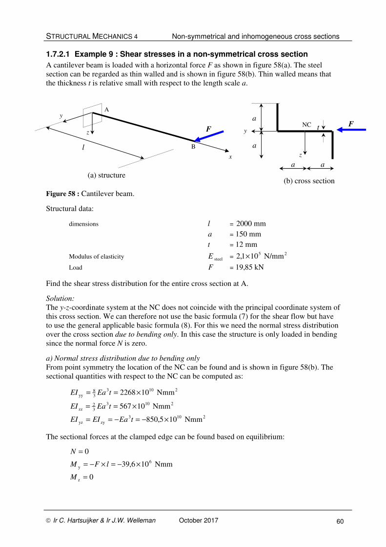
STRUCTURAL MECHANICS 4 Non-symmetrical and inhomogeneous cross sections
Ir C. Hartsuijker & Ir J.W. Welleman October 2017 60
1.7.2.1 Example 9 : Shear stresses in a non-symmetrical cross section
A cantilever beam is loaded with a horizontal force F as shown in figure 58(a). The steel
section can be regarded as thin walled and is shown in figure 58(b). Thin walled means that
the thickness t is relative small with respect to the length scale a.
Figure 58 : Cantilever beam.
Structural data:
dimensions l = mm2000
a = mm150
t = mm12
Modulus of elasticity steelE = 25 N/mm101,2 ×
Load F = kN85,19
Find the shear stress distribution for the entire cross section at A.
Solution:
The y-z-coordinate system at the NC does not coincide with the principal coordinate system of
this cross section. We can therefore not use the basic formula (7) for the shear flow but have
to use the general applicable basic formula (8). For this we need the normal stress distribution
over the cross section due to bending only. In this case the structure is only loaded in bending
since the normal force N is zero.
a) Normal stress distribution due to bending only
From point symmetry the location of the NC can be found and is shown in figure 58(b). The
sectional quantities with respect to the NC can be computed as:
2103
zyyz
2103
32
zz
2103
38
yy
Nmm105,850
Nmm10567
Nmm102268
×−=−==
×==
×==
tEaEIEI
tEaEI
tEaEI
The sectional forces at the clamped edge can be found based on equilibrium:
0
Nmm106,39
0
z
6
y
=
×−=×−=
=
M
lFM
N
(a) structure
x
l
z F
A
B
y
F y
z
a
t
a a
NC
(b) cross section
a
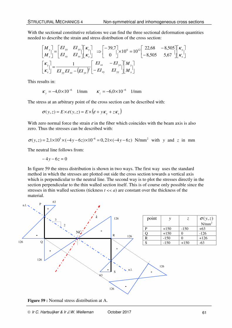
STRUCTURAL MECHANICS 4 Non-symmetrical and inhomogeneous cross sections
Ir C. Hartsuijker & Ir J.W. Welleman October 2017 61
With the sectional constitutive relations we can find the three sectional deformation quantities
needed to describe the strain and stress distribution of the cross section:
( )
−
−
−=
−
−=×
−⇒
=
z
y
yyzy
yzzz
2
yzzzyyz
y
z
y126
z
y
zzzy
yzyy
z
y
1
67,5505,8
505,868,221010
0
7,39
M
M
EIEI
EIEI
EIEIEI
EIEI
EIEI
M
M
κ
κ
κ
κ
κ
κ
This results in:
1/mm100,61/mm100,4 66 −− ×−=×−= zy κκ
The stress at an arbitrary point of the cross section can be described with:
( )zy),(),( κκεεσ zyEzyEzy ++×=×=
With zero normal force the strain ε in the fiber which coincides with the beam axis is also
zero. Thus the stresses can be described with:
5 6 2( , ) 2,1 10 ( 4 6 ) 10 0, 21 ( 4 6 ) N/mm with and in mmy z y z y z y zσ −= × × − − × = × − −
The neutral line follows from:
064 =−− zy
In figure 59 the stress distribution is shown in two ways. The first way uses the standard
method in which the stresses are plotted out side the cross section towards a vertical axis
which is perpendicular to the neutral line. The second way is to plot the stresses directly in the
section perpendicular to the thin walled section itself. This is of course only possible since the
stresses in thin walled sections (tickness t << a) are constant over the thickness of the
material.
Figure 59 : Normal stress distribution at A.
2
3
n.l.
n.l.
k
63
126
126
126
+
+
+
-
-
-
-
+
NC
P
Q
R
S
point y z ),( zyσ
N/mm2
P +150 -150 +63
Q +150 0 -126
R -150 0 +126
S -150 +150 -63
126
126
126
63
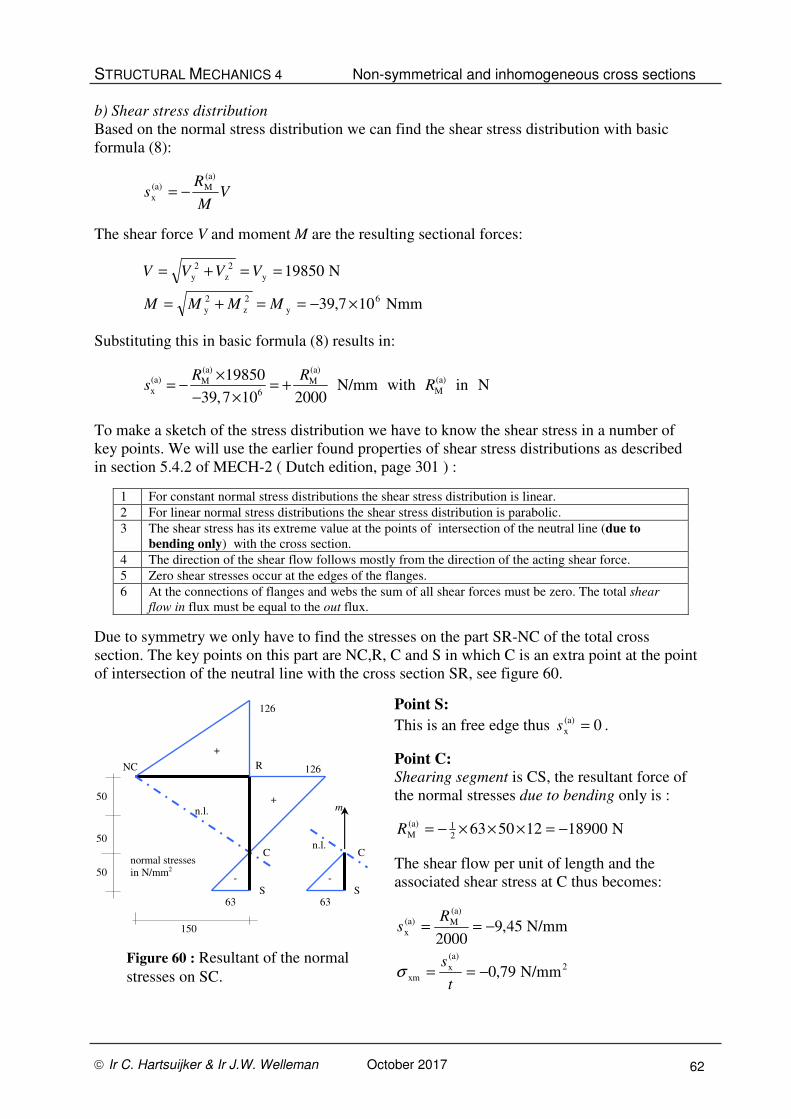
STRUCTURAL MECHANICS 4 Non-symmetrical and inhomogeneous cross sections
Ir C. Hartsuijker & Ir J.W. Welleman October 2017 62
b) Shear stress distribution
Based on the normal stress distribution we can find the shear stress distribution with basic
formula (8):
VM
Rs
(a)
M(a)
x −=
The shear force V and moment M are the resulting sectional forces:
Nmm107,39
N19850
6
y
2
z
2
y
y
2
z
2
y
×−==+=
==+=
MMMM
VVVV
Substituting this in basic formula (8) results in:
(a) (a)
(a) (a)M Mx M6
19850N/mm with in N
39,7 10 2000
R Rs R
×= − = +
− ×
To make a sketch of the stress distribution we have to know the shear stress in a number of
key points. We will use the earlier found properties of shear stress distributions as described
in section 5.4.2 of MECH-2 ( Dutch edition, page 301 ) :
1 For constant normal stress distributions the shear stress distribution is linear.
2 For linear normal stress distributions the shear stress distribution is parabolic.
3 The shear stress has its extreme value at the points of intersection of the neutral line (due to
bending only) with the cross section.
4 The direction of the shear flow follows mostly from the direction of the acting shear force.
5 Zero shear stresses occur at the edges of the flanges.
6 At the connections of flanges and webs the sum of all shear forces must be zero. The total shear
flow in flux must be equal to the out flux.
Due to symmetry we only have to find the stresses on the part SR-NC of the total cross
section. The key points on this part are NC,R, C and S in which C is an extra point at the point
of intersection of the neutral line with the cross section SR, see figure 60.
Point S:
This is an free edge thus 0(a)
x =s .
Point C:
Shearing segment is CS, the resultant force of
the normal stresses due to bending only is :
N1890012506321(a)
M −=×××−=R
The shear flow per unit of length and the
associated shear stress at C thus becomes:
2
(a)
x
xm
(a)
M(a)
x
N/mm79,0
N/mm45,92000
−==
−==
t
s
Rs
σ
+
R
S
126
126
63
C
+
-
normal stresses
in N/mm2
NC
Figure 60 : Resultant of the normal
stresses on SC.
S 63
C
-
m n.l.
n.l.
50
50
50
150
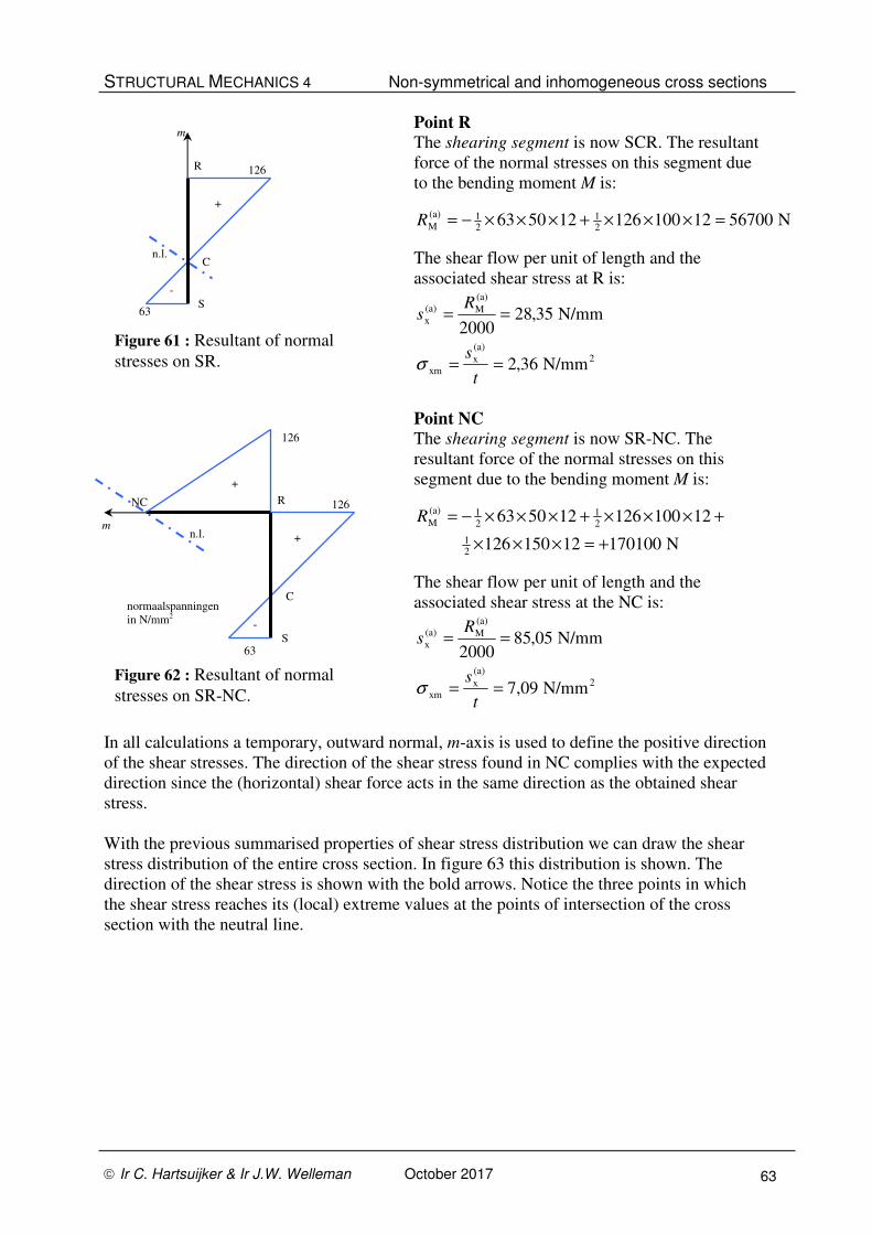
STRUCTURAL MECHANICS 4 Non-symmetrical and inhomogeneous cross sections
Ir C. Hartsuijker & Ir J.W. Welleman October 2017 63
+
R
S
126
126
63
C
+
-
normaalspanningen
in N/mm2
NC
Figure 61 : Resultant of normal
stresses on SR.
S 63
C
-
m
n.l.
n.l.
R 126
+
m
Figure 62 : Resultant of normal
stresses on SR-NC.
Point R
The shearing segment is now SCR. The resultant
force of the normal stresses on this segment due
to the bending moment M is:
N567001210012612506321
21(a)
M =×××+×××−=R
The shear flow per unit of length and the
associated shear stress at R is:
2
(a)
x
xm
(a)
M(a)
x
N/mm36,2
N/mm35,282000
==
==
t
s
Rs
σ
Point NC
The shearing segment is now SR-NC. The
resultant force of the normal stresses on this
segment due to the bending moment M is:
N17010012150126
12100126125063
21
21
21(a)
M
+=×××
+×××+×××−=R
The shear flow per unit of length and the
associated shear stress at the NC is:
2
(a)
x
xm
(a)
M(a)
x
N/mm09,7
N/mm05,852000
==
==
t
s
Rs
σ
In all calculations a temporary, outward normal, m-axis is used to define the positive direction
of the shear stresses. The direction of the shear stress found in NC complies with the expected
direction since the (horizontal) shear force acts in the same direction as the obtained shear
stress.
With the previous summarised properties of shear stress distribution we can draw the shear
stress distribution of the entire cross section. In figure 63 this distribution is shown. The
direction of the shear stress is shown with the bold arrows. Notice the three points in which
the shear stress reaches its (local) extreme values at the points of intersection of the cross
section with the neutral line.

STRUCTURAL MECHANICS 4 Non-symmetrical and inhomogeneous cross sections
Ir C. Hartsuijker & Ir J.W. Welleman October 2017 64
Figure 63 : Shear stress distribution.
Since the normal stress distribution is linear for all parts of the cross section, the shear stress
distribution will be parabolic on all segments. For segment SR the distribution can be found
rather quickly since the parabolic distribution reaches its extreme value at C. At D therefore
the shear stress must again be zero!
c) Exact shear stress distribution
The exact expression for the shear stress distribution can also be obtained by using basic
formula (8). As an example we will derive this expression for segment SR.
To describe the shear stress distribution for segment SR we use a shearing segment SW with a
local (outward) normal m-axis as shown in figure 64.
The linear stress distribution on SR can be written
as a function of m with:
mm150
18963)( +−=σ
This normal stress distribution is due to bending
only. This is an important requirement when using
basic formula (8).
The resulting normal force due to bending on the shearing area SW is:
( ) mmmtmR
t
××+−=×= ∫ 12)(63d)(21
0
(a)
M σσ
Combining these two expressings results in:
2
2
1(a)
M25
18975612
150
1896363 mmmmR +−=××
+−+−=
2
3
n.l.
n.l.
NC
P
Q
R
S
2,36
2,36
0,79
7,09
4,73
2,36
0,79
z
y
50
50
50 V = 19850 N
Shear stress distribution in N/mm2
C
D
50
50
50
Figure 64 : Normal stress on SR.
S 63
C
-
m-as
n.l.
σ
σ(m)
m
W
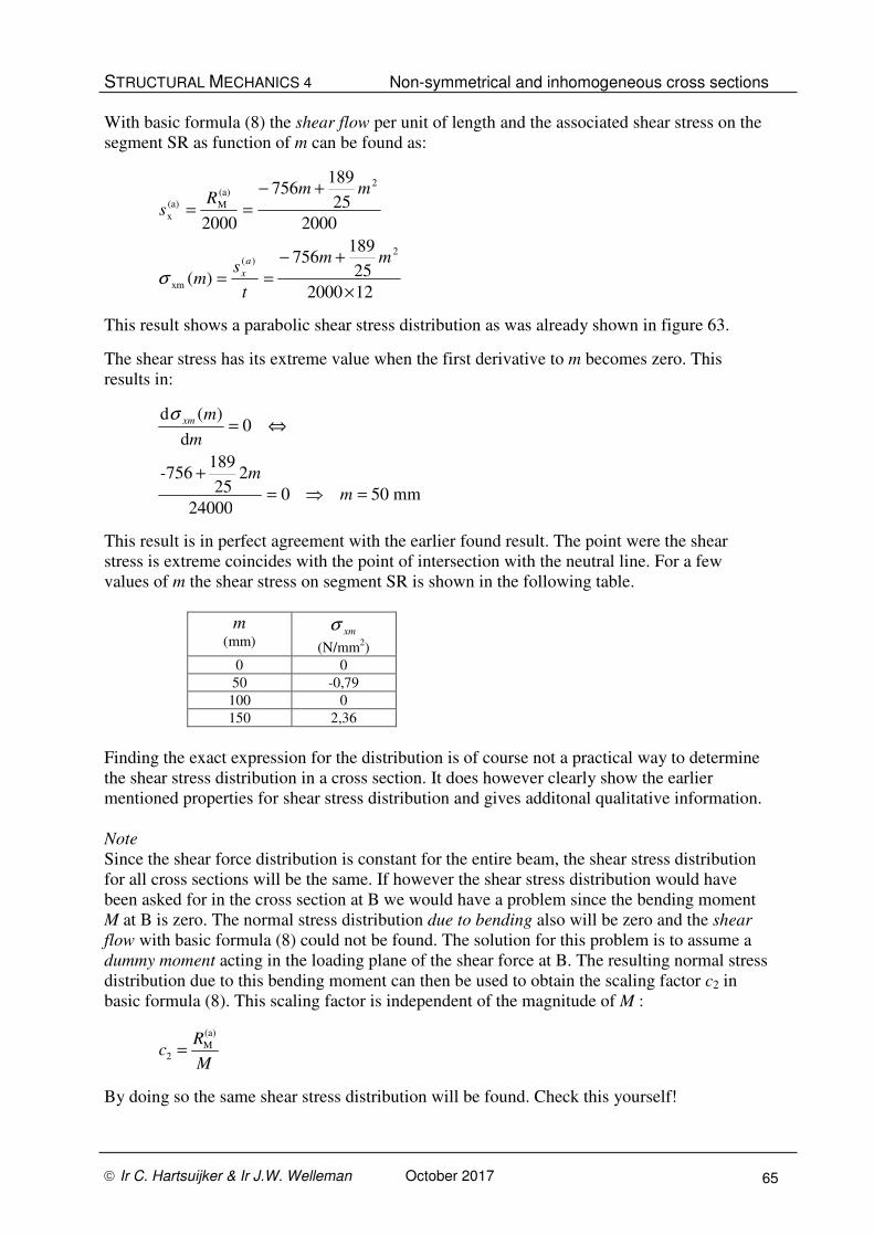
STRUCTURAL MECHANICS 4 Non-symmetrical and inhomogeneous cross sections
Ir C. Hartsuijker & Ir J.W. Welleman October 2017 65
With basic formula (8) the shear flow per unit of length and the associated shear stress on the
segment SR as function of m can be found as:
122000
25
189756
)(
2000
25
189756
2000
2)(
xm
2(a)
M(a)
x
×
+−==
+−==
mm
t
sm
mmR
s
a
xσ
This result shows a parabolic shear stress distribution as was already shown in figure 63.
The shear stress has its extreme value when the first derivative to m becomes zero. This
results in:
mm50024000
225
189756
0d
)(d
=⇒=+
⇔=
m
m-
m
mxmσ
This result is in perfect agreement with the earlier found result. The point were the shear
stress is extreme coincides with the point of intersection with the neutral line. For a few
values of m the shear stress on segment SR is shown in the following table.
m (mm)
xmσ
(N/mm2)
0 0
50 -0,79
100 0
150 2,36
Finding the exact expression for the distribution is of course not a practical way to determine
the shear stress distribution in a cross section. It does however clearly show the earlier
mentioned properties for shear stress distribution and gives additonal qualitative information.
Note
Since the shear force distribution is constant for the entire beam, the shear stress distribution
for all cross sections will be the same. If however the shear stress distribution would have
been asked for in the cross section at B we would have a problem since the bending moment
M at B is zero. The normal stress distribution due to bending also will be zero and the shear
flow with basic formula (8) could not be found. The solution for this problem is to assume a
dummy moment acting in the loading plane of the shear force at B. The resulting normal stress
distribution due to this bending moment can then be used to obtain the scaling factor c2 in
basic formula (8). This scaling factor is independent of the magnitude of M :
(a)
M2
Rc
M=
By doing so the same shear stress distribution will be found. Check this yourself!
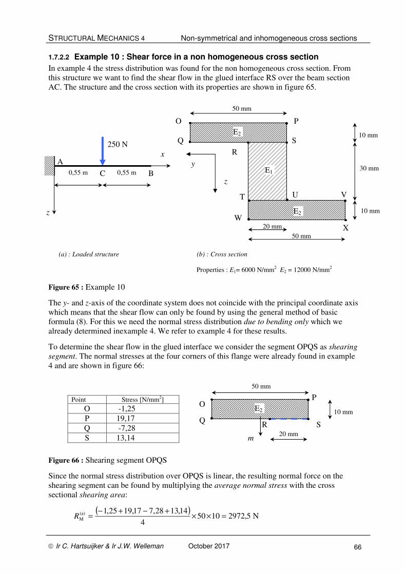
STRUCTURAL MECHANICS 4 Non-symmetrical and inhomogeneous cross sections
Ir C. Hartsuijker & Ir J.W. Welleman October 2017 66
1.7.2.2 Example 10 : Shear force in a non homogeneous cross section
In example 4 the stress distribution was found for the non homogeneous cross section. From
this structure we want to find the shear flow in the glued interface RS over the beam section
AC. The structure and the cross section with its properties are shown in figure 65.
(a) : Loaded structure (b) : Cross section
Properties : E1= 6000 N/mm2 E2 = 12000 N/mm
2
Figure 65 : Example 10
The y- and z-axis of the coordinate system does not coincide with the principal coordinate axis
which means that the shear flow can only be found by using the general method of basic
formula (8). For this we need the normal stress distribution due to bending only which we
already determined inexample 4. We refer to example 4 for these results.
To determine the shear flow in the glued interface we consider the segment OPQS as shearing
segment. The normal stresses at the four corners of this flange were already found in example
4 and are shown in figure 66:
Point Stress [N/mm2]
O -1,25
P 19,17
Q -7,28
S 13,14
Figure 66 : Shearing segment OPQS
Since the normal stress distribution over OPQS is linear, the resulting normal force on the
shearing segment can be found by multiplying the average normal stress with the cross
sectional shearing area:
( )
N5,297210504
14,1328,717,1925,1(a)
M =××+−+−
=R
250 N
0,55 m 0,55 m
x
z
A
B
y E1
E2
10 mm
30 mm
20 mm
z C
E2
10 mm
50 mm
50 mm
O P
Q S
T V
W
X
R
U
10 mm E2
50 mm
O P
S R Q
20 mm m
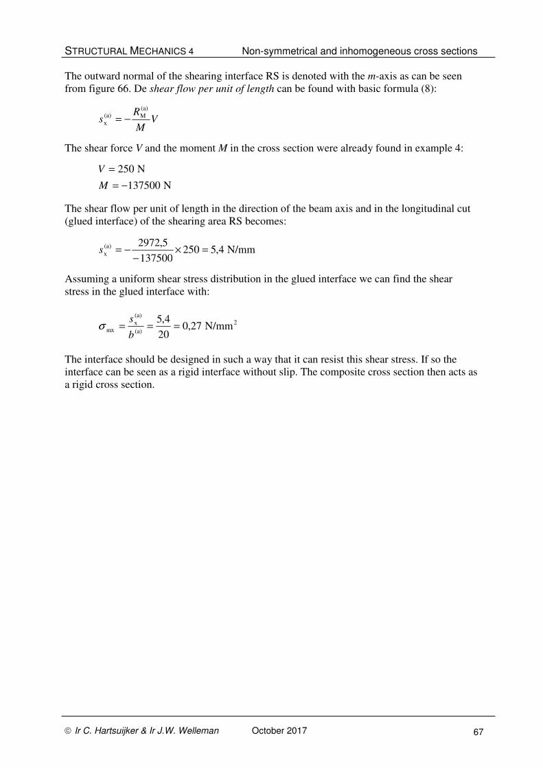
STRUCTURAL MECHANICS 4 Non-symmetrical and inhomogeneous cross sections
Ir C. Hartsuijker & Ir J.W. Welleman October 2017 67
The outward normal of the shearing interface RS is denoted with the m-axis as can be seen
from figure 66. De shear flow per unit of length can be found with basic formula (8):
VM
Rs
(a)
M(a)
x −=
The shear force V and the moment M in the cross section were already found in example 4:
N137500
N250
−=
=
M
V
The shear flow per unit of length in the direction of the beam axis and in the longitudinal cut
(glued interface) of the shearing area RS becomes:
N/mm4,5250137500
5,2972(a)
x =×−
−=s
Assuming a uniform shear stress distribution in the glued interface we can find the shear
stress in the glued interface with:
2
(a)
(a)
x
mx N/mm27,020
4,5===
b
sσ
The interface should be designed in such a way that it can resist this shear stress. If so the
interface can be seen as a rigid interface without slip. The composite cross section then acts as
a rigid cross section.
STRUCTURAL MECHANICS 4 Non-symmetrical and inhomogeneous cross sections
Ir C. Hartsuijker & Ir J.W. Welleman October 2017 68
1.7.3 Shear force center for thin walled non-symmeyrical cross sections
In case of thin walled cross sections we assume constant shear stresses over the thickness of
the material. The resultant force of these shear stresses is of course equal to the acting shear
force in the cross section. However its line of action will in most cases not act in the normal
force center NC but in the so-called shear force center SC, see also section 5.5 of MECH-2 .
The shear force center is defined as:
The shear force center SC is a point in the plane of the cross section were the shear force
must be applied in order to cause shear stresses without torsion.
In case of rotation symmetrical cross section the shear force center SC conincides with the
normal force center NC. For arbitrary shaped cross sections however this will not be the case.
If the cross section has an axis of symmetry, the shear force center SC will be located on this
axis. For a number of standard sections this has been illustrated in MECH-2 (Dutch edition,
page 331).
In this section we will show how to find the location of the shear force center SC in case of
arbitrary shaped thin walled cross sections without an axis of symmetry. The procedure which
has to be followed is an extension of the outlined method of the previous sections. The
neccesary steps to find the shear force center are:
Step 1 : Find for an arbitrary shear force the shear stress distribution in the cross section.
Determine the line of action of the resulting shear force and denote this force with its
line of action as R1 .
Step 2 : Find for a second shear force which is different with respect to its direction to
the one from step 1, the shear stress distribution on the cross section.
Determine the line of action of the resulting shear force and denote this force with its
line of action as R2 .
Step 3 : The shear force center is the point of intersection of the two lines R1 and R2 .
Since we try to find the point of intersection of two lines of action it is essential to choose two
shear forces which are not parallel to each other.
The term arbitrary also means that we can choose a clever or intelligent special set of shear
forces since we are free in our assumption of the directions and the magnitude of the set of
shear forces as long as these two shear forces are not parellel to each other.
If we choose two unity shear forces which acts in the direction of the coordinate system we
can simplify the calculations as will be illustrated in the following example.
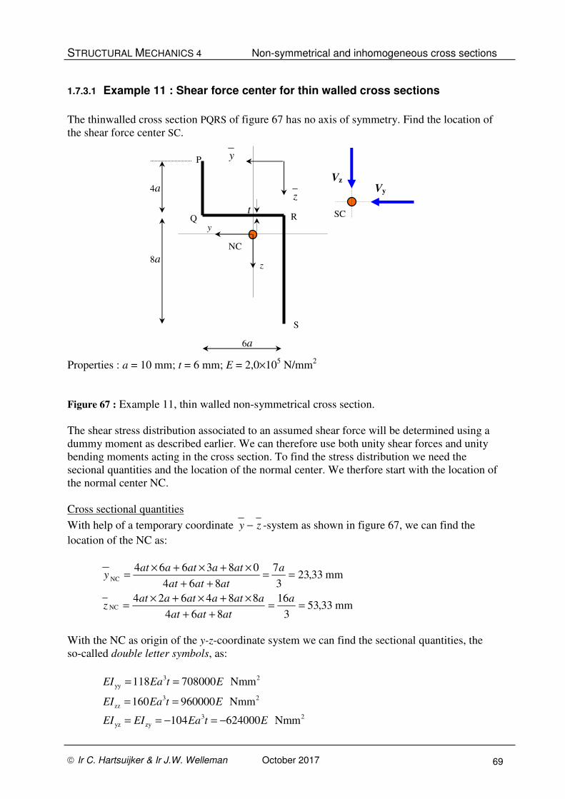
STRUCTURAL MECHANICS 4 Non-symmetrical and inhomogeneous cross sections
Ir C. Hartsuijker & Ir J.W. Welleman October 2017 69
1.7.3.1 Example 11 : Shear force center for thin walled cross sections
The thinwalled cross section PQRS of figure 67 has no axis of symmetry. Find the location of
the shear force center SC.
Properties : a = 10 mm; t = 6 mm; E = 2,0×10⁵ N/mm
2
Figure 67 : Example 11, thin walled non-symmetrical cross section.
The shear stress distribution associated to an assumed shear force will be determined using a
dummy moment as described earlier. We can therefore use both unity shear forces and unity
bending moments acting in the cross section. To find the stress distribution we need the
secional quantities and the location of the normal center. We therfore start with the location of
the normal center NC.
Cross sectional quantities
With help of a temporary coordinate zy − -system as shown in figure 67, we can find the
location of the NC as:
mm33,533
16
864
884624
mm33,233
7
864
083664
NC
NC
==++
×+×+×=
==++
×+×+×=
a
atatat
aataataatz
a
atatat
ataataaty
With the NC as origin of the y-z-coordinate system we can find the sectional quantities, the
so-called double letter symbols, as:
3 2
yy
3 2
zz
3 2
yz zy
118 708000 Nmm
160 960000 Nmm
104 624000 Nmm
EI Ea t E
EI Ea t E
EI EI Ea t E
= =
= =
= = − = −
Vy
y
z 4a
t
6a
8a
Vz
SC
NC
y
z
P
Q R
S

STRUCTURAL MECHANICS 4 Non-symmetrical and inhomogeneous cross sections
Ir C. Hartsuijker & Ir J.W. Welleman October 2017 70
The shear stress distribution can only be found using the general method described in section
1.7.2 since the section is non symmetrical. In this method we need a normal stress distribution
due to bending only. We will use a dummy moment in the same loading plane as the acting
shear force. The magnitude of this moment is of no importance. We therefore choose a unity
moment as dummy.
To find the location of the shear force center we have to compute two shear stress
distributions. The first distribution is the result of a unity shear force Vy and the associated
(dummy) unity moment My . The second distribution is the result of a unity shear force Vz
with the associated (dummy) unity moment Mz. All calculations can be made using MAPLE.
Load case 1 : Nmm0,0
0,1;N
0,0
0,1
=
=
z
y
z
y
M
M
V
V
Load case 2 : Nmm0,1
0,0;N
0,1
0,0
=
=
z
y
z
y
M
M
V
V
With this “intelligent” choice we can simplify basic formula (8) to:
b
R
b
s
RVM
Rs
(a)
M
(a)
x
xm
(a)
M
(a)
M(a)
x
−==
−=−=
σ
( modified formula 8 )
With this expression we can easily find the shear flow and shear stress distribution due to a
unity shear force.
Normal stress distribution for load case 1
In the same manner as presented in example 9 the normal stress distribution can be found
starting with the sectional constitutive relation:
( )
−
−
−=
−
−×=
⇒
=
0
0,11
960624
624708100,2
0
0,1
0
0,1
yyzy
yzzz
2
yzzzyyz
y
z
y8
z
y
zzzy
yzyy
EIEI
EIEI
EIEIEI
EIEI
EIEI
κ
κ
κ
κ
κ
κ
The components of the curvature results from the above expression as:
1/mm10107474,01/mm10165344,0 1010 −− ×=×= zy κκ
The stress in any point of the cross section can subsequently be found with:
( )zy),(),( κκεεσ zyEzyEzy ++×=×=
The strain ε in the fiber through the normal center NC is zero since the normal force is zero.
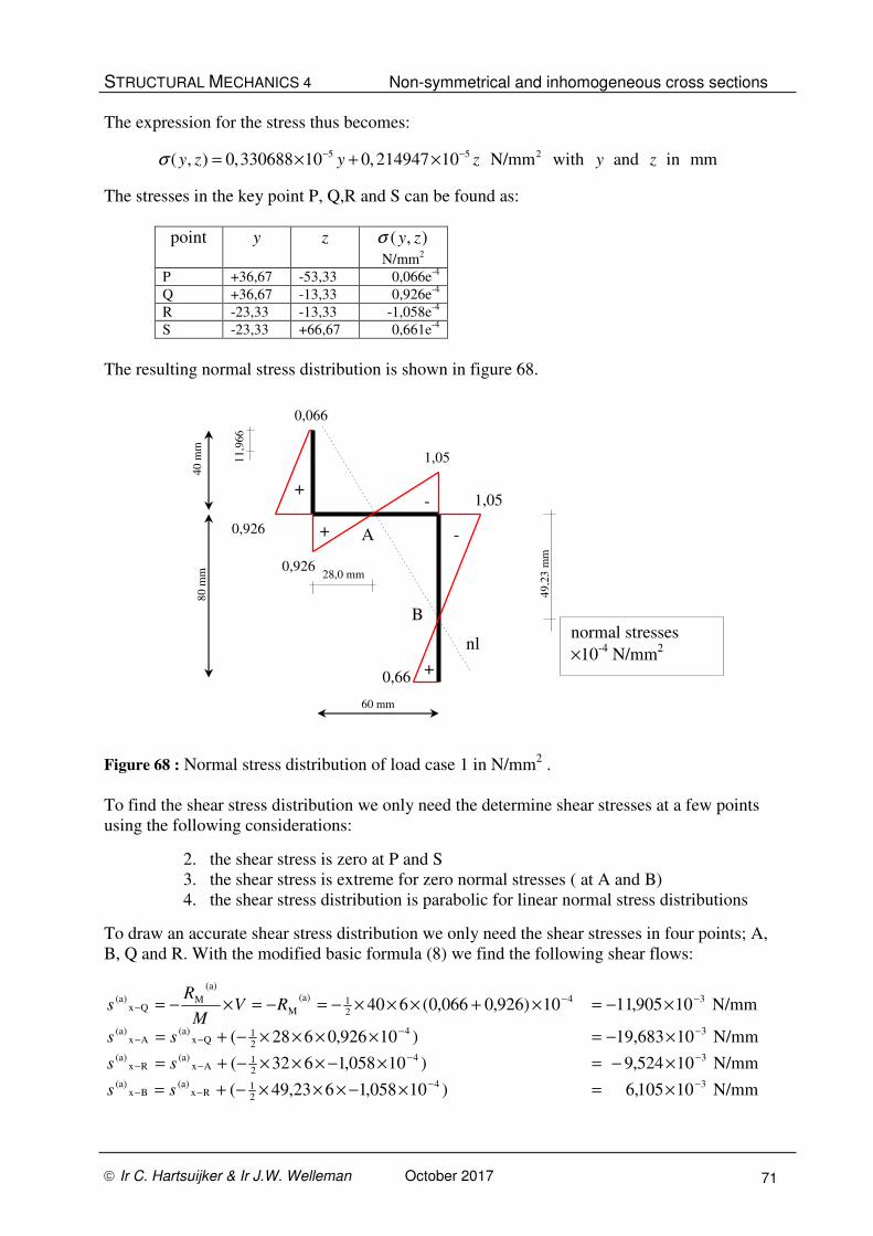
STRUCTURAL MECHANICS 4 Non-symmetrical and inhomogeneous cross sections
Ir C. Hartsuijker & Ir J.W. Welleman October 2017 71
The expression for the stress thus becomes:
5 5 2( , ) 0,330688 10 0, 214947 10 N/mm with and in mmy z y z y zσ − −= × + ×
The stresses in the key point P, Q,R and S can be found as:
point y z ),( zyσ
N/mm2
P +36,67 -53,33 0,066e-4
Q +36,67 -13,33 0,926e-4
R -23,33 -13,33 -1,058e-4
S -23,33 +66,67 0,661e-4
The resulting normal stress distribution is shown in figure 68.
Figure 68 : Normal stress distribution of load case 1 in N/mm2 .
To find the shear stress distribution we only need the determine shear stresses at a few points
using the following considerations:
2. the shear stress is zero at P and S
3. the shear stress is extreme for zero normal stresses ( at A and B)
4. the shear stress distribution is parabolic for linear normal stress distributions
To draw an accurate shear stress distribution we only need the shear stresses in four points; A,
B, Q and R. With the modified basic formula (8) we find the following shear flows:
N/mm10105,6)10058,1623,49(
N/mm10524,9)10058,1632(
N/mm10683,19)10926,0628(
N/mm10905,1110)926,0066,0(640
34
21
Rx(a)
Bx(a)
34
21
Ax(a)
Rx(a)
34
21
Qx(a)
Ax(a)
34
21(a)
M
(a)
MQx
(a)
−−−−
−−−−
−−−−
−−−
×=×−×××−+=
×−=×−×××−+=
×−=××××−+=
×−=×+×××−=−=×−=
ss
ss
ss
RVM
Rs
60 mm
normal stresses
×10-4
N/mm2
0,066
0,926
0,926
1,05
1,05
0,66
nl
A
B
11,9
66
40 m
m
80 m
m
28,0 mm
49,2
3 m
m
+ -
+
+
-

STRUCTURAL MECHANICS 4 Non-symmetrical and inhomogeneous cross sections
Ir C. Hartsuijker & Ir J.W. Welleman October 2017 72
The shear flow distribution is shown in figure 69. The arrows show the direction in which the
shear flow actually works.
Figure 69 : Shear flow distribution of load case 1.
For each segment of the cross section the resultant force can be found by integrating the shear
flow function and multiply this result with the constant thickness of the segment. In order to
find the expressions for the shear flow distributions for each of the segments DQ, QR and RS
only the shear flow in Q and R are needed.
For segment PQ we choose the variable x from P towards Q and find for the resulting shear
force:
N1693,04
)(4
0
PQ21
P
PQ −=
×
−+××−= ∫
a
dxa
xxtR
σσσ
For segment QR we choose the variable x from Q to R and find for the resulting shear force:
N0,16
)(6
0
QR21
QQ-x(a)QR −=
×
−+××−= ∫
a
dxa
xxtsR
σσσ
For segment RS we choose the variable x from R to R and find for the resulting shear force:
N1693,08
)(8
0
RS21
RR-x(a)RS =
×
−+××−= ∫
a
dxa
xxtsR
σσσ
The sum of the horizontal and vertical components of the shear force are indeed equal to the
applied shear forces Vy (1,0) en Vz (0,0).
The direction of the shear flow in segment QR can be found directly from the acting shear
force or with help of a local outward normal m-axis. Draw a small sketch to check this
yourself!
60 mm
shear flow
×10-3
N/mm
11,9
11,9
9,5
4
nl
A
B
11,9
66
40 m
m
80 m
m
28 mm
49,2
3 m
m
19,7
9,5
4
P
Q
R
S
6,1

STRUCTURAL MECHANICS 4 Non-symmetrical and inhomogeneous cross sections
Ir C. Hartsuijker & Ir J.W. Welleman October 2017 73
The resulting forces on each segment are shown in figure 70. Based on equilibrium the
resulting force and its line of action can be determined. This is also shown in figure 70. The
resulting force for load case 1 is of course equal to the unity shear force Vy .
Figure 70 : Line of action of the resulting shear force for load case 1.
The shear force center, we are looking for, must lie somewhere on this line of action. To find
the exact location we need a second line of action. At the point of intersection of these two
lines we find the location of the shear force center. The whole procedure has therefore to be
repeated for load case 2. We will only show the brief results since this is a repetition of steps.
Normal stress distribution for load case 2
With the (dummy) unity moment Mz we can find the sectional defomations with the sectional
constitutive relation:
( )
−
−
−=
0,1
01
yyzy
yzzz
2
yzzzyyz
y
EIEI
EIEI
EIEIEIκ
κ
The components of the curvature become:
1/mm10121941,01/mm10107474,0 1010 −− ×=×= zy κκ
The expression for the normal stress distribution will become:
mminenmetN/mm10243882,010214947,0),( 255 zyzyzy −− ×+×=σ
The stresses at key points P, Q,R and S can be found as:
point y z ),( zyσ
N/mm2
P +36,67 -53,33 -0,513e-4
Q +36,67 -13,33 0,463e-4
R -23,33 -13,33 -0,827e-4
S -23,33 +66,67 1,124e-4
60 mm
0,1693 N
40 m
m
80 m
m
P
Q R
S
0,1693 N
1,0 N
1,0 N
line of action of the resultant
of all shear stresses in the
cross section. e=10,16 mm
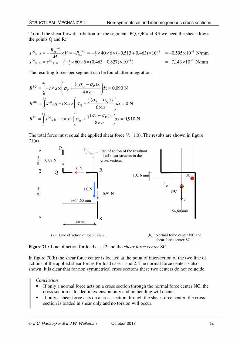
STRUCTURAL MECHANICS 4 Non-symmetrical and inhomogeneous cross sections
Ir C. Hartsuijker & Ir J.W. Welleman October 2017 74
To find the shear flow distribution for the segments PQ, QR and RS we need the shear flow at
the points Q and R:
N/mm10143,7)10)827,0463,0(660(
N/mm10595,010)463,0513,0(640
34
21
Qx(a)
Rx(a)
34
21(a)
M
(a)
MQx
(a)
−−−−
−−−
×=×−×××−+=
×−=×+−×××−=−=×−=
ss
RVM
Rs
The resulting forces per segment can be found after integration:
N090,04
)(4
0
PQ21
P
PQ =
×
−+××−= ∫
a
dxa
xxtR
σσσ
N06
)(6
0
QR21
QQ-x(a)QR =
×
−+××−= ∫
a
dxa
xxtsR
σσσ
N910,08
)(8
0
RS21
RR-x(a)RS =
×
−+××−= ∫
a
dxa
xxtsR
σσσ
The total force must equal the applied shear force Vz (1,0). The results are shown in figure
71(a).
Figure 71 : Line of action for load case 2 and the shear force center SC.
In figure 70(b) the shear force center is located at the point of intersection of the two line of
actions of the applied shear forces for load case 1 and 2. The normal force center is also
shown. It is clear that for non symmetrical cross sections these two centers do not coincide.
Conclusion
• If only a normal force acts on a cross section through the normal force center NC, the
cross section is loaded in extension only and no bending will occur.
• If only a shear force acts on a cross section through the shear force center, the cross
section is loaded in shear only and no torsion will occur.
60 mm
0,91 N
40 m
m
80 m
m
P
Q R
S
0,09 N
0 N
1,0 N
line of action of the resultant
of all shear stresses in the
cross section.
e=54,60 mm
54,60 mm
(a) : Line of action of load case 2. (b) : Normal force center NC and
shear force center SC
10,16 mm
NC
y
z
SC

STRUCTURAL MECHANICS 4 Non-symmetrical and inhomogeneous cross sections
Ir C. Hartsuijker & Ir J.W. Welleman October 2017 75
APPENDIX A
The proof that the curvature can be considered as a first order tensor will be given below. In
order to do so we have to examine the effect of a rotation of the coorinate system on the
expression of the strain field in a cross section.
y z( , )y z y zε ε κ κ= + +
For a given point P, see the figure below, we can find the relation between its position in the
original y-z-coordinate system and the rotated y z− -coordinate system as:
Figure 72 : Coordinate transformation due to a rotation.
cos sin
sin cos
y y z
z y z
α α
α α
= +
= − + and the inverse :
cos sin
sin cos
y y z
z y z
α α
α α
= −
= +
These latter relations are the tensor transformation rules for first order tensors. The strain in
the y-z-coordinate system can thus be expressed in terms of the rotated coordinate system
with:
( ) ( )
( ) ( )
y z
y z
y z y z
y z
( , )
cos sin sin cos
cos sin sin cos
y z y z
y z y z
y z
y z
ε ε κ κ
ε α α κ α α κ
ε κ α κ α κ α κ α
ε κ κ
= + +
= + − + +
= + + + − +
= + +
From this latter expression follows that the transformation of the curvature complies with the
transformation rule of a first order tensor from which we can deduce that the curvature is a
first order tensor.
More or less in the same way we can proof that also the moment vector M is a first order
tensor which will be shown on the next page.
STRUCTURAL MECHANICS 4 Non-symmetrical and inhomogeneous cross sections
Ir C. Hartsuijker & Ir J.W. Welleman October 2017 76
To do so we investigate the effect of a rotation on the expressions of the sectional forces,
normal force N and moment M. The previous found relations also hold in the rotated
coordinate system, thus:
( , )d
( , )d
( , )d
y
z
N y z A
M y y z A
M z y z A
σ
σ
σ
=
=
=
∫
∫
∫
In het original system we find:
( , )d
( , )d
( , )d
y
y
N y z A
M y y z A
M z y z A
σ
σ
σ
=
=
=
∫
∫
∫
By using the inverse relation for the coordinate transformation from the previous page,
cos sin
sin cos
y y z
z y z
α α
α α
= −
= +
we find:
( ) ( )
( ) ( )
( , )d
( cos sin ) ( , )d
( , )d cos ( , )d sin
cos sin
( sin cos ) ( , )d
( , )d sin ( , )d cos
sin cos
y
y z
z
y z
N y z A
M y z y z A
y y z A z y z A
M M
M y z y z A
y y z A z y z A
M M
σ
α α σ
σ α σ α
α α
α α σ
σ α σ α
α α
=
= −
= −
= −
= +
= +
= +
∫
∫
∫ ∫
∫
∫ ∫
The components of the moment M transform like:
cos sin
sin cos
y y z
z y z
M M M
M M M
α α
α α
= −
= +
This transformation is exactly the same as the transformation rule for a first order tensor.
Both the curvature and the moment vector can be regarded as first order tensors..

STRUCTURAL MECHANICS 4 Non-symmetrical and inhomogeneous cross sections
Ir C. Hartsuijker & Ir J.W. Welleman October 2017 77
APPENDIX B
The moment distribution in the xy- and the xz-plane of a statically indeterminate element
exhibits a coupling if the boundary conditions in both planes are not the same. As an example
we consider the same structure as in figure 19-2 and will vary the boundary conditions. The
beam is loaded with a constant distributed load qy and qz and the two differential equations to
be solved are:
2
2
"''
"''
zz y yz z
y
yy zz yz
yz y yy z
z
yy zz yz
EI q EI qu
EI EI EI
EI q EI qu
EI EI EI
−=
−
− +=
−
The general solution of these ODE are:
4 3 2
1 23 42
4 3 2
1 23 42
( )
24( ) 6 4
( )
24( ) 6 4
zz y yz z
y
yy zz yz
yz y yy z
z
yy zz yz
EI q EI q x C x C xu C x C
EI EI EI
EI q EI q x D x D xu D x D
EI EI EI
−= + + + +
−
− += + + + +
−
Situation 1:
The beam is fully clamped at the left end at x = 0 and simply supported at the right end x = l.
The eight boundary conditions can be described as:
0 : ( 0; 0; 0; 0)
: ( 0; 0; 0; 0)
y z y z
y z y z
x u u
x l u u M M
ϕ ϕ= = = = =
= = = = =
Solving the ODE we find for the moment distributions:
2 218
2 218
( ) (4 5 )
( ) (4 5 )
y y
z z
M x q x xl l
M x q x xl l
= − − +
= − − +
In this case we find the normal moment distribution which we could also have obtained with a
simple analysis in one plane. The moment at the clamped edge is:
218
218
(0)
(0)
y y
z z
M q l
M q l
= −
= −
Situation 2:
The beam is only fully clamped in the xz-plane at the left end at x = 0. In the xy-plane the
beam is at this location simply supported. At the right end x = l the beam is in both the xy- and
the xz-plane simply supported. The eight boundary conditions can be described as:
0 : ( 0; 0; 0; 0)
: ( 0; 0; 0; 0)
y z y z
y z y z
x u u M
x l u u M M
ϕ= = = = =
= = = = =
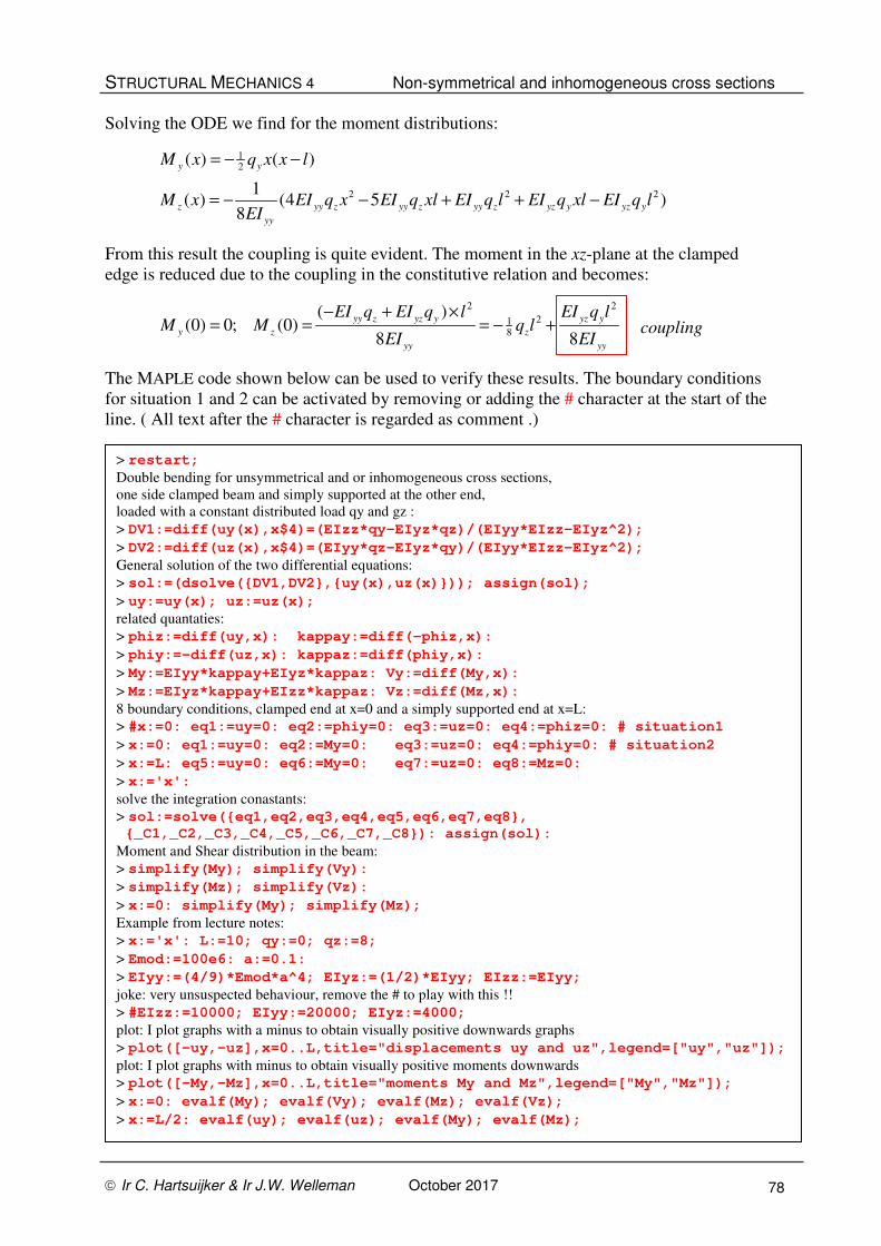
STRUCTURAL MECHANICS 4 Non-symmetrical and inhomogeneous cross sections
Ir C. Hartsuijker & Ir J.W. Welleman October 2017 78
Solving the ODE we find for the moment distributions:
12
2 2 2
( ) ( )
1( ) (4 5 )
8
y y
z yy z yy z yy z yz y yz y
yy
M x q x x l
M x EI q x EI q xl EI q l EI q xl EI q lEI
= − −
= − − + + −
From this result the coupling is quite evident. The moment in the xz-plane at the clamped
edge is reduced due to the coupling in the constitutive relation and becomes:
2 2
218
( )(0) 0; (0)
8 8
yy z yz y yz y
y z z
yy yy
EI q EI q l EI q lM M q l
EI EI
− + ×= = = − +
The MAPLE code shown below can be used to verify these results. The boundary conditions
for situation 1 and 2 can be activated by removing or adding the # character at the start of the
line. ( All text after the # character is regarded as comment .)
> restart;
Double bending for unsymmetrical and or inhomogeneous cross sections,
one side clamped beam and simply supported at the other end,
loaded with a constant distributed load qy and gz :
> DV1:=diff(uy(x),x$4)=(EIzz*qy-EIyz*qz)/(EIyy*EIzz-EIyz^2);
> DV2:=diff(uz(x),x$4)=(EIyy*qz-EIyz*qy)/(EIyy*EIzz-EIyz^2);
General solution of the two differential equations:
> sol:=(dsolve({DV1,DV2},{uy(x),uz(x)})); assign(sol);
> uy:=uy(x); uz:=uz(x);
related quantaties:
> phiz:=diff(uy,x): kappay:=diff(-phiz,x):
> phiy:=-diff(uz,x): kappaz:=diff(phiy,x):
> My:=EIyy*kappay+EIyz*kappaz: Vy:=diff(My,x):
> Mz:=EIyz*kappay+EIzz*kappaz: Vz:=diff(Mz,x):
8 boundary conditions, clamped end at x=0 and a simply supported end at x=L:
> #x:=0: eq1:=uy=0: eq2:=phiy=0: eq3:=uz=0: eq4:=phiz=0: # situation1
> x:=0: eq1:=uy=0: eq2:=My=0: eq3:=uz=0: eq4:=phiy=0: # situation2
> x:=L: eq5:=uy=0: eq6:=My=0: eq7:=uz=0: eq8:=Mz=0:
> x:='x':
solve the integration conastants:
> sol:=solve({eq1,eq2,eq3,eq4,eq5,eq6,eq7,eq8},
{_C1,_C2,_C3,_C4,_C5,_C6,_C7,_C8}): assign(sol):
Moment and Shear distribution in the beam:
> simplify(My); simplify(Vy):
> simplify(Mz); simplify(Vz):
> x:=0: simplify(My); simplify(Mz);
Example from lecture notes:
> x:='x': L:=10; qy:=0; qz:=8;
> Emod:=100e6: a:=0.1:
> EIyy:=(4/9)*Emod*a^4; EIyz:=(1/2)*EIyy; EIzz:=EIyy;
joke: very unsuspected behaviour, remove the # to play with this !!
> #EIzz:=10000; EIyy:=20000; EIyz:=4000;
plot: I plot graphs with a minus to obtain visually positive downwards graphs
> plot([-uy,-uz],x=0..L,title="displacements uy and uz",legend=["uy","uz"]);
plot: I plot graphs with minus to obtain visually positive moments downwards
> plot([-My,-Mz],x=0..L,title="moments My and Mz",legend=["My","Mz"]);
> x:=0: evalf(My); evalf(Vy); evalf(Mz); evalf(Vz);
> x:=L/2: evalf(uy); evalf(uz); evalf(My); evalf(Mz);
coupling

STRUCTURAL MECHANICS 4 Non-symmetrical and inhomogeneous cross sections
Ir C. Hartsuijker & Ir J.W. Welleman October 2017 79
2. ASSIGNMENTS
2.1 Cross sectional properties
All specified problems are related to the determination of the cross sectional quantities of
homogeneous non-symmetrical cross sections.
Problem 1
Question:
a) Centre of gravity Z.
b) The second moments of area for the given
coordinate system.
c) The second moments of area for a coordinate
system which is rotated by 45o .
d) The second moments of area for a coordinate
system with its origin at C.
Problem 2
Question:
a) Centre of gravity
b) , , yy zz yzI I I
c) Principal directions
d) Principal second moments of area (moments of inertia)

STRUCTURAL MECHANICS 4 Non-symmetrical and inhomogeneous cross sections
Ir C. Hartsuijker & Ir J.W. Welleman October 2017 80
Problem 3
Given: 3' ' 1/12z zI bh= ×
Question:
a) Check with Steiner’s parallel theorem.
b) Compute the magnitude of '' ''z zI
Problem 4
Question:
a) Centre of gravity
b) The second moments of area : yzzzyy ,, III
d) The principal directions
e) Principal second moments of area (moments of inertia)
Problem 5
Question:
a) Centre of gravity
b) , , yy zz yzI I I
c) Pricipal directions
d) Principal second moments of
area (moments of inertia)
e) The coordinate system for
which the magnitude of ' 'y zI
is at largest.
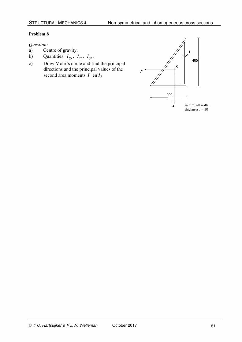
STRUCTURAL MECHANICS 4 Non-symmetrical and inhomogeneous cross sections
Ir C. Hartsuijker & Ir J.W. Welleman October 2017 81
Problem 6
Question:
a) Centre of gravity.
b) Quantities: , , yy zz yzI I I .
c) Draw Mohr’s circle and find the principal
directions and the principal values of the
second area moments 1 2 en I I
in mm, all walls
thickness t = 10
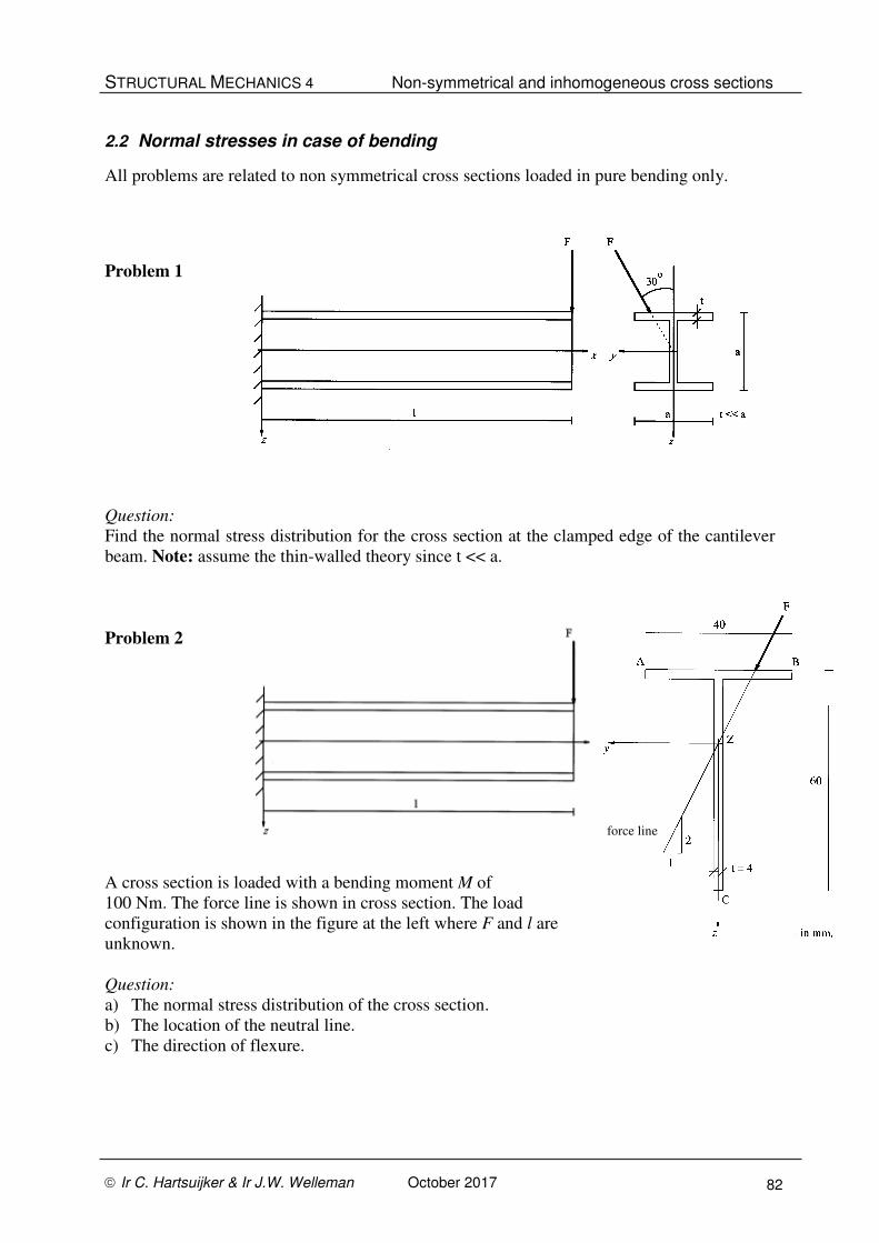
STRUCTURAL MECHANICS 4 Non-symmetrical and inhomogeneous cross sections
Ir C. Hartsuijker & Ir J.W. Welleman October 2017 82
2.2 Normal stresses in case of bending
All problems are related to non symmetrical cross sections loaded in pure bending only.
Problem 1
Question:
Find the normal stress distribution for the cross section at the clamped edge of the cantilever
beam. Note: assume the thin-walled theory since t << a.
Problem 2
A cross section is loaded with a bending moment M of
100 Nm. The force line is shown in cross section. The load
configuration is shown in the figure at the left where F and l are
unknown.
Question:
a) The normal stress distribution of the cross section.
b) The location of the neutral line.
c) The direction of flexure.
force line
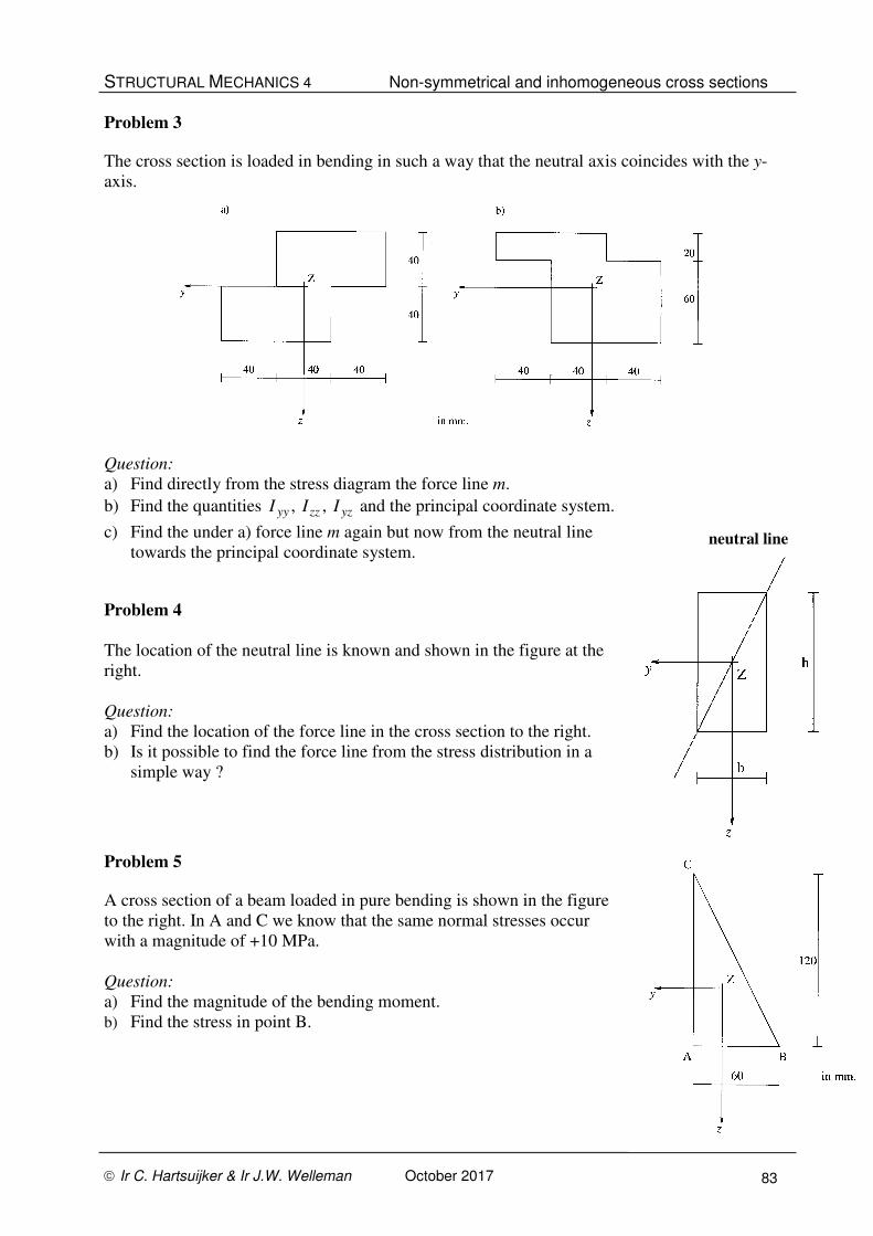
STRUCTURAL MECHANICS 4 Non-symmetrical and inhomogeneous cross sections
Ir C. Hartsuijker & Ir J.W. Welleman October 2017 83
Problem 3
The cross section is loaded in bending in such a way that the neutral axis coincides with the y-
axis.
Question:
a) Find directly from the stress diagram the force line m.
b) Find the quantities , , yy zz yzI I I and the principal coordinate system.
c) Find the under a) force line m again but now from the neutral line
towards the principal coordinate system.
Problem 4
The location of the neutral line is known and shown in the figure at the
right.
Question:
a) Find the location of the force line in the cross section to the right.
b) Is it possible to find the force line from the stress distribution in a
simple way ?
Problem 5
A cross section of a beam loaded in pure bending is shown in the figure
to the right. In A and C we know that the same normal stresses occur
with a magnitude of +10 MPa.
Question:
a) Find the magnitude of the bending moment.
b) Find the stress in point B.
neutral line

STRUCTURAL MECHANICS 4 Non-symmetrical and inhomogeneous cross sections
Ir C. Hartsuijker & Ir J.W. Welleman October 2017 84
Problem 6
A cantilever beam with a I-section type of HE 160A is loaded by two forces and y zF F as
shown in the figure.
Properties:
4 4yy
4 4
max
HE 160A
612 10 mm
1673 10 mm
100 MPa
160 mm; 152 mm; 3000 mm
zz
I
I
b h l
σ
= ×
= ×
=
= = =
Question:
Find the maximum values for and y zF F for which holds: zy FF = .
Problem 7
A beam with a cross section as shown in the figure is
loaded in pure bending. The largest compressive
stress is –50 MPa and the largest tensile stress is +70
MPa.
Question:
a) Find the magnitude and the direction of the
moment in this cross section.

STRUCTURAL MECHANICS 4 Non-symmetrical and inhomogeneous cross sections
Ir C. Hartsuijker & Ir J.W. Welleman October 2017 85
Problem 8
A thin walled section is loaded with:
2
2
80
52
y
z
M a t
M a t
= + σ
= + σ
Question:
a) Find the stresses at the corner points A, B, C
and D.
b) Find the location of the neutral line.
c) Determine the second moment of area yyI in
the direction perpendicular to the neutral line.
d) Check the stress at A which results when using the stress formula.
Problem 9
Beam AB with a L-section as shown in the figure is clamped at A with the vertical (web) of
the section. At B the beam is loaded with a vertical force F = 500 N. The force acts at the
normal force centre NC of the thin walled cross section.
Question:
a) Draw the normal stress distribution for a cross section at A. Put the values and the signs in
the graph.
b) Find the location of the shear force center S.C. and the torsional moment in this section.
c) Calculate the displacement of the normal center NC at B.
d) Find the maximum shear stress and its location in a cross section.
NC
Properties:
GPa200
mm105,13
mm105,22
44
yz
44
zzyy
=
×−=
×==
E
I
II

STRUCTURAL MECHANICS 4 Non-symmetrical and inhomogeneous cross sections
Ir C. Hartsuijker & Ir J.W. Welleman October 2017 86
NC
NC
Problem 10
A cantilever beam with a L-section 100 / 100 / 10 is clamped at the vertical plane A-D. The
normal force center NC at the end B is attached to a tension rod BC in such a way that the
cross section at B can only move in vertical direction. The deformation of the tension rod BC
is negligible. The vertical load of 1000 N is applied at the normal force centre. Use a Young’s
modulus E = 210 GPa. The cross section can NOT be regarded as thin walled.
Question:
a) Find the normal force in the tension rod in such a way that the cantilever beam AB only
shows a vertical displacement. HINT : Use the pseudo-load.
b) Show that for each cross section over AB the neutral line is a horizontal line.
c) Draw the normal stress distribution due to the bending moment at the clamped support,
put the values and signs in the graph.
d) Find the maximum shear stress in this cross section due to the total applied shear force.
For this computation you may regard the cross section as thin walled.
e) Find the torsional moment in beam AB and show its direction.
NOTE:
The influence of the torsional moment on the shear stresses is not asked for but you can
add these to the shear stress found due to shear only.

STRUCTURAL MECHANICS 4 Non-symmetrical and inhomogeneous cross sections
Ir C. Hartsuijker & Ir J.W. Welleman October 2017 87
2.3 Normal stresses due to bending and extension
The following assignments all deal with unsymmetrical and or inhomogeneous cross sections loaded
in bending and/or extension.
Problem 1
A column is loaded by an excentric
load as shown in the figure.
Question:
a) Determine the stress distribution of
the normal stress in cross sesction
C-C for F = 10 kN. The point of
application of this force is point A
as shown in the top view.
b) The same question but now for a
force which acts in point B as
shown in the top view.
Problem 2
Answer the same questions for a thin
walled column with a cross section as
shown in the figure to the right.
Top view
cross section C-C
dimensions in mm
dimensions in mm
t= 10 mm
dimensions in mm.
a) b)
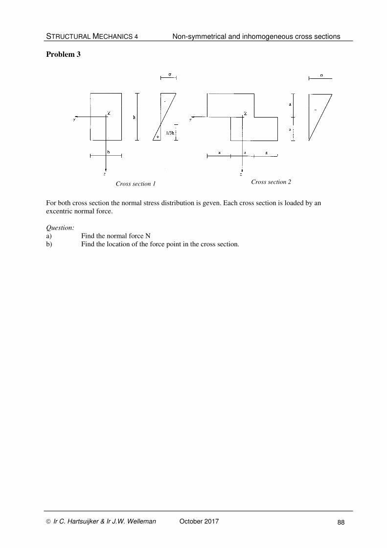
STRUCTURAL MECHANICS 4 Non-symmetrical and inhomogeneous cross sections
Ir C. Hartsuijker & Ir J.W. Welleman October 2017 88
Problem 3
For both cross section the normal stress distribution is geven. Each cross section is loaded by an
excentric normal force.
Question:
a) Find the normal force N
b) Find the location of the force point in the cross section.
Cross section 1 Cross section 2

STRUCTURAL MECHANICS 4 Non-symmetrical and inhomogeneous cross sections
Ir C. Hartsuijker & Ir J.W. Welleman October 2017 89
2.4 Inhomogeneous cross sections loaded in extension
Problem 1
A concrete column of 4 meters in length is reinforced
with a steel HEA-section. The column must transfer
a compressive force of 160 kN.
200 GPa 14 GPast bE E= =
questions:
a) The distribution of normal forces over the cross-
section
b) The shortening of the column
c) Determine the maximal compressive force on the
column when
concrete steel10 MPa and 160 MPaσ = σ =
Problem 2
The shown concrete cross-section is reinforced with 8
steel bars 25∅ .
210 GPa 14 GPas bE E= =
The allowed stress in the concrete and steel is 10 MPa
and 160 MPa respectively.
questions:
a) the maximal compressive force on the column
b) The point of application of this compressive force
in the case where no bending occurs in the column.
Problem 3
A column of length 3 ml = with a square cross-section is
built up of four squares of 40 × 40 mm2 of different materials.
1 330 GPa 100 GPaE E= =
2 460 GPa 200 GPaE E= =
questions:
a) Determine the elastic center of gravity for this
inhomogenuous cross-section (Normal centre).
b) If for all the materials the maximal compressive stress is
100 MPa, what is the maximal compressive force F on the
column that acts on the elastic center of gravity.
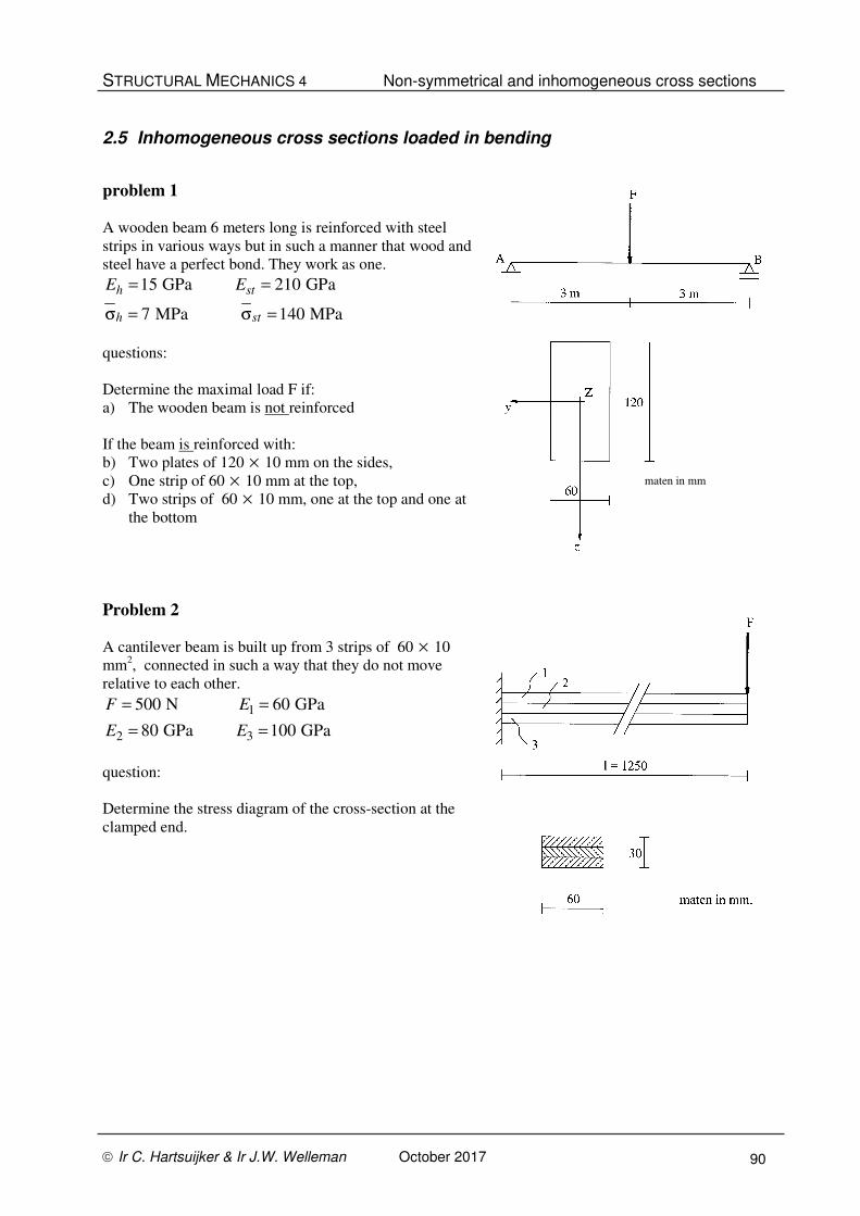
STRUCTURAL MECHANICS 4 Non-symmetrical and inhomogeneous cross sections
Ir C. Hartsuijker & Ir J.W. Welleman October 2017 90
2.5 Inhomogeneous cross sections loaded in bending
problem 1
A wooden beam 6 meters long is reinforced with steel
strips in various ways but in such a manner that wood and
steel have a perfect bond. They work as one.
15 GPa 210 GPa
7 MPa 140 MPa
h st
h st
E E= =
σ = σ =
questions:
Determine the maximal load F if:
a) The wooden beam is not reinforced
If the beam is reinforced with:
b) Two plates of 120 × 10 mm on the sides,
c) One strip of 60 × 10 mm at the top,
d) Two strips of 60 × 10 mm, one at the top and one at
the bottom
Problem 2
A cantilever beam is built up from 3 strips of 60 × 10
mm2, connected in such a way that they do not move
relative to each other.
1
2 3
500 N 60 GPa
80 GPa 100 GPa
F E
E E
= =
= =
question:
Determine the stress diagram of the cross-section at the
clamped end.
maten in mm
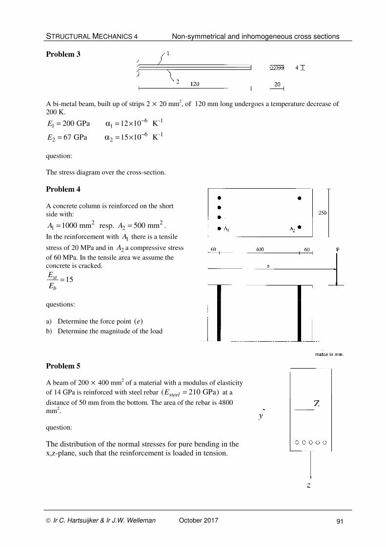
STRUCTURAL MECHANICS 4 Non-symmetrical and inhomogeneous cross sections
Ir C. Hartsuijker & Ir J.W. Welleman October 2017 91
Problem 3
A bi-metal beam, built up of strips 2 × 20 mm2, of 120 mm long undergoes a temperature decrease of
200 K. 6 -1
1 1
6 -12 2
200 GPa 12 10 K
67 GPa 15 10 K
E
E
−
−
= α = ×
= α = ×
question:
The stress diagram over the cross-section.
Problem 4
A concrete column is reinforced on the short
side with: 2 2
1 21000 mm resp. 500 mmA A= = .
In the reinforcement with 1A there is a tensile
stress of 20 MPa and in 2A a compressive stress
of 60 MPa. In the tensile area we assume the
concrete is cracked.
15st
b
E
E=
questions:
a) Determine the force point ( )e
b) Determine the magnitude of the load
Problem 5
A beam of 200 × 400 mm2 of a material with a modulus of elasticity
of 14 GPa is reinforced with steel rebar ( 210 GPa)steelE = at a
distance of 50 mm from the bottom. The area of the rebar is 4800
mm2.
question:
The distribution of the normal stresses for pure bending in the
x,z-plane, such that the reinforcement is loaded in tension.
STRUCTURAL MECHANICS 4 Non-symmetrical and inhomogeneous cross sections
Ir C. Hartsuijker & Ir J.W. Welleman October 2017 92
Problem 6
If the beam from the previous exercise is made from reinforced concrete, the low tensile strength of
the concrete must be taken into account. To do this most of the time a fully cracked cross-section is
assumed in the tensile zone, which means no strength remains there in the concrete. Determine in that
case the distribution of the normal stresses.

STRUCTURAL MECHANICS 4 Non-symmetrical and inhomogeneous cross sections
Ir C. Hartsuijker & Ir J.W. Welleman October 2017 93
2.6 Core
Problem 1
Determine the core of the shown cross-section:
a) analytically
b) grafically
Determine furthermore:
c) The stresses occuring in corners A, B and C due to a
bending moment MyM =
d) The force line when the neutral axis coincides with the y-axis
Problem 2
Determine the core for these three cross-sections
Problem 3
a) Determine for these cross-sections the core.
b) Determine the stress distribution if the cross-section is loaded with a compressive force in A.
2
4a
3 3

STRUCTURAL MECHANICS 4 Non-symmetrical and inhomogeneous cross sections
Ir C. Hartsuijker & Ir J.W. Welleman October 2017 94
Problem 4
The given cross-section transfers a compressive force of
a 100kN.
questions:
a) Determine the location of the force point.
b) Draw the stress distribution.
Problem 5
The drawn profile is the cross-section of a simply
supported concrete beam with a length l loaded with a
variable uniformly distributed load.
Indicate how pretension cables have to be placed in
this cross-section such that the maximal bending
moment is maximized. l = 8 m.
Problem 6
The drawn cross-section transfers a bending
moment 150 kNmzM = .
questions:
a) Determine the core of the cross-section
b) Draw the normal stress distribution with
values and signs.
c) For what direction of the force line is the
deflection direction vertical?

STRUCTURAL MECHANICS 4 Non-symmetrical and inhomogeneous cross sections
Ir C. Hartsuijker & Ir J.W. Welleman October 2017 95
Problem 7
Two beams:
a) Determine the bending stresses occurring in the middle cross-section of two simply supported
beams loaded with a uniformly distributed load of 2kN/m. The length of the beams is 2 meters and
the cross-sections are as the shown profiles in a and b above.
b) How must the beams be rotated around their axis such that the occurring bending stresses are
minimized?
c) How must the beams be rotated around their axis such that the direction of deflection is vertical?
Problem 8
A hollow thin-walled column has a cross-section as
indicated.
questions:
a) Determine the moments of inertia for the given
coordinate system through the center of gravity.
b) Draw the core of this cross-section.
c) If it is given that the neutral line due to a normal
force of 2 kN coincides with AE, sketch the stress
distribution and determine the location of the force
point.
300
300
300
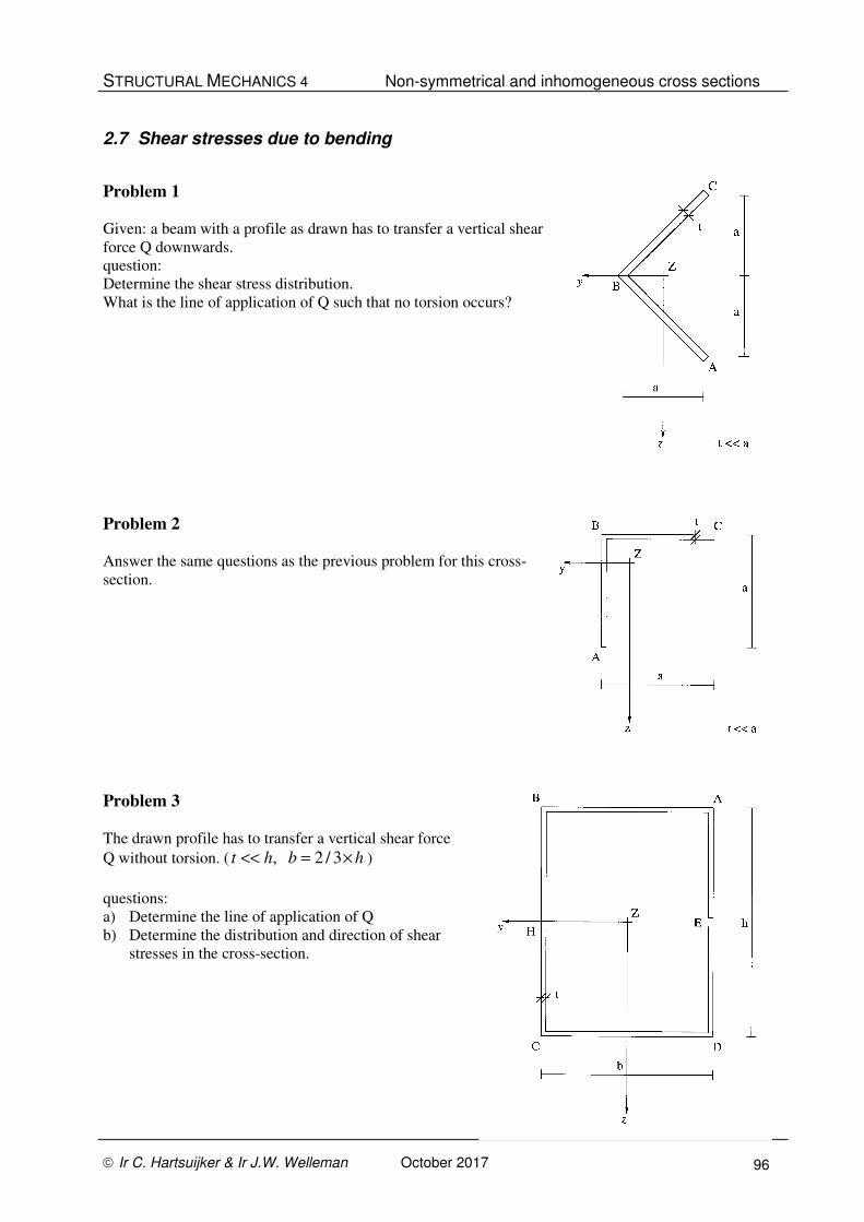
STRUCTURAL MECHANICS 4 Non-symmetrical and inhomogeneous cross sections
Ir C. Hartsuijker & Ir J.W. Welleman October 2017 96
2.7 Shear stresses due to bending
Problem 1
Given: a beam with a profile as drawn has to transfer a vertical shear
force Q downwards.
question:
Determine the shear stress distribution.
What is the line of application of Q such that no torsion occurs?
Problem 2
Answer the same questions as the previous problem for this cross-
section.
Problem 3
The drawn profile has to transfer a vertical shear force
Q without torsion. ( , 2 / 3t h b h<< = × )
questions:
a) Determine the line of application of Q
b) Determine the distribution and direction of shear
stresses in the cross-section.
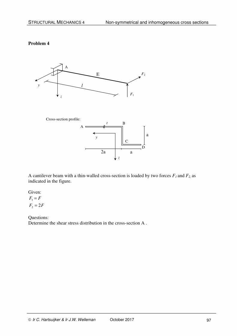
STRUCTURAL MECHANICS 4 Non-symmetrical and inhomogeneous cross sections
Ir C. Hartsuijker & Ir J.W. Welleman October 2017 97
Problem 4
A cantilever beam with a thin-walled cross-section is loaded by two forces F1 and F2, as
indicated in the figure.
Given:
F F=1
2 2F F=
Questions:
Determine the shear stress distribution in the cross-section A .
t
z
2a
z
a
a y
F2
F1
A
E
l y
Cross-section profile: B
C
D
A