
Module 3 ENERGY EFFICIENCY IN ELECTRICAL SYSTEMS
257
c c ENERGY EFFICIENCY IN ELECTRICAL SYSTEMS Module 3 Sustainable and Renewable Energy Development Authority Power Division First Edition’2019
Transcript of Module 3 ENERGY EFFICIENCY IN ELECTRICAL SYSTEMS

c
c
ENERGY EFFICIENCY
IN
ELECTRICAL SYSTEMS
Module 3
Sustainable and Renewable Energy Development Authority
Power Division
First Edition’2019

P

Preamble In order to ensure energy efficiency and conservation and to determine the future course
of action, Sustainable and Renewable Energy Development Authority (SREDA) has
developed the Energy Efficiency & Conservation Master Plan up to 2030 in 2016.
According to this plan, the target of energy saving has been set 15% & 20% per GDP by
2020 & 2030 respectively which will be achieved by the use of energy efficient
machinery and equipment as well as by improving energy management system in the
demand side .
In order to achieve the above mentioned target & to ensure the energy efficiency and
conservation in industrial & commercial sector, SREDA has formulated the Energy
Audit Regulation’2018. Based on this regulation, SREDA will conduct the Energy
Auditor Certification Examination to create energy auditors and energy managers in
Bangladesh.
SREDA has prepared the following modules as reading material for four paper
examinations in cooperation with various National and Foreign partner organizations.
Module No Examination
Paper
Subject
Module 01 Paper 01 Fundamentals of Energy Management and Energy
Audit
Module 02 Paper 02 Energy Efficiency in Thermal Systems
Module 03 Paper 03 Energy Efficiency in Electrical Systems
Module 04 Paper 04 Energy Performance Assessment for Equipment
and Utility Systems
This module 03 on Energy Efficiency in Electrical Systems is the reading material for the
preparation of Paper 03 Examination for prospective candidates.
We hope that these modules will also act as valuable resource for practicing engineers in
comprehending and implementing energy efficiency measures in the facilities.
It is the first iteration of these modules. It will be a living document which can be
reviewed and revised time to time according to the evolution of the technology and
industry. Any suggestion and comments (please email to [email protected] ) on the
contents of those modules will be highly appreciated.


Table of Contents Chapter 1: Electrical Systems ........................................................................................................... 1
1.1 Introduction to Electric Power Supply Systems .......................................................................... 1
1.2 Electricity billing .......................................................................................................................... 8
1.3 Electrical load management and maximum demand control .................................................. 10
1.4 Power factor improvement and benefits .................................................................................... 12
1.5 System distribution losses .......................................................................................................... 21
1.6 Harmonics and its Effects.......................................................................................................... 22
1.7 A Glossary of Basic Electrical Terms ........................................................................................ 28
Chapter 2: Electrical Motors ........................................................................................................... 30
2.1 Introduction ................................................................................................................................ 30
2.2 Motor Types ................................................................................................................................ 30
2.2.1 Induction Motors................................................................................................................. 30
2.2.2 Direct-Current Motors ........................................................................................................ 32
2.2.3 Synchronous Motors ........................................................................................................... 32
2.3 Motor Characteristics ................................................................................................................ 32
2.3.1 Motor Speed ........................................................................................................................ 32
2.3.2 Volts/Hz Relationship ......................................................................................................... 33
...................................................................................................................................................... 34
2.3.3 Power Factor ....................................................................................................................... 34
2.3.4 Motor Efficiency Parameters .............................................................................................. 34
2.4 Motors Selection ......................................................................................................................... 35
2.4.1 Field Tests for Determining Efficiency .............................................................................. 36
2.5 Energy-Efficient Motors ............................................................................................................ 39
2.5.1 Stator and Rotor I2 R Losses ............................................................................................... 40
2.5.2 Core Loses ........................................................................................................................... 40
2.5.3 Friction and Wind age Losses ............................................................................................ 40
2.5.4 Stray Load-Losses ............................................................................................................... 40
2.6 Factors Affecting Energy Efficiency & Minimising Motor Losses in operation .................... 41
2.6.1 Power Supply Quality.......................................................................................................... 41
2.6.2 Motor Loading..................................................................................................................... 45
2.6.3 Power Factor Correction .................................................................................................... 47
2.6.4 Maintenance ........................................................................................................................ 48
2.6.5 Age ....................................................................................................................................... 48
2.6.6 Rewinding Effects on Energy Efficiency ........................................................................... 49
2.6.7 Speed Control of AC Induction Motors.............................................................................. 49
2.6.8 Other operating concerns ................................................................................................... 59
2.6.9 Transmission Efficiency ..................................................................................................... 60

2.6.10 Soft Starters ....................................................................................................................... 60
2.7 Case Studies ............................................................................................................................... 61
Chapter 3: COMPRESSED AIRSYSTEMS ................................................................................. 63
3.1 Introduction ................................................................................................................................ 63
3.2 Compressor Types ...................................................................................................................... 63
3.3 Positive Displacement Compressors .......................................................................................... 63
3.3.1 Reciprocating Compressors ................................................................................................ 63
3.3.2 Rotary Compressors ............................................................................................................ 64
3.4 Centrifugal Compressors ........................................................................................................... 65
3.5 System Components ................................................................................................................... 66
3.6 Compressor Performance .......................................................................................................... 66
3.7 Efficient Compressor Operation ................................................................................................ 68
3.7.1 Reciprocating Compressors ................................................................................................ 68
3.7.2 Centrifugal Compressors .................................................................................................... 69
3.7.3 Screw Compressors ............................................................................................................. 69
3.8 Energy Efficiency Practices In Compressed Air Systems ........................................................ 70
3.8.1 Location of Compressors .................................................................................................... 70
3.8.2 Dust Free Air Intake ........................................................................................................... 70
3.8.3 Dry Air Intake ..................................................................................................................... 71
3.8.4 Pre-Cooled Air Intake ......................................................................................................... 72
3.8.5 Elevation .............................................................................................................................. 72
3.8.6 Cooling Water Circuit ......................................................................................................... 72
3.8.7 Efficacy of Inter and After Coolers .................................................................................... 74
3.8.8 Pressure Settings ................................................................................................................. 75
3.8.9 Blowers in place of Compressed Air System ...................................................................... 78
3.8.10 Capacity Control of Compressors ..................................................................................... 78
3.8.11 Avoiding Misuse of Compressed Air ................................................................................ 80
3.8.12 Avoiding Air Leaks and Energy Wastage ........................................................................ 81
3.8.13 Compressor Capacity Assessment .................................................................................... 84
3.8.14 Line Moisture Separator and Traps ................................................................................. 86
3.8.15 Compressed Air Filter ....................................................................................................... 87
3.8.16 Regulators ......................................................................................................................... 87
3.8.17 Lubricators ........................................................................................................................ 87
3.8.18 Air Dryers .......................................................................................................................... 87
3.8.19 Air Receivers ..................................................................................................................... 88
3.8.20 Capacity Utilisation ........................................................................................................... 89
Chapter 4: FANS AND BLOWERS ............................................................................................... 90
4.1 Introduction .............................................................................................................................. 90
4.2 Fan Types .................................................................................................................................. 90

4.3 Common Blower Types............................................................................................................. 93
4.4 Fan Performance Evaluation and Efficient System Operation .......................................... 94
4.5 Fan Design and Selection Criteria ......................................................................................... 98
4.6 Flow Control Strategies ......................................................................................................... 103
4.7 Fan Performance Assessment .............................................................................................. 108
4.8 Energy Savings Opportunities .............................................................................................. 112
4.9 Case Study on Pressure Drop Reduction Across the Bag Filter ....................................... 113
4.10 Computational Fluid Dynamics ......................................................................................... 114
Chapter 5: HVAC and Refrigeration System ............................................................................. 118
5.1 Introduction ............................................................................................................................ 118
5.2 Psychrometrics and Air-Conditioning Processes ............................................................... 118
5.3 Types of Refrigeration System .............................................................................................. 122
5.4 Common Refrigerants and Properties ................................................................................. 126
5.5 Compressor Types and Application ...................................................................................... 127
5.6 Selection of a Suitable Refrigeration System ...................................................................... 131
5.7 Performance Assessment of Refrigeration Plants .................................................................. 132
5.8 Factors Affecting Performance & Energy Efficiency of Refrigeration Plants ............... 134
5.9 Performance Assessment of window, split and package air conditioning units Air
Conditioners ................................................................................................................................... 139
5.10 Cold Storage Systems ........................................................................................................... 140
5.11 Heat Pumps aim (heir Applications ................................................................................... 141
5.12 Ventilation Systems .............................................................................................................. 143
5.13 Ice Bank Systems.................................................................................................................. 143
5.14 Humidification Systems ....................................................................................................... 144
5.15 Energy Saving Opportunities ................................................................................................. 145
5.16 Case Study: Screw Compressor Application ..................................................................... 146
Chapter 6: Pumps And Pumping System .................................................................................... 149
6.1 Pump Types ............................................................................................................................. 149
6.2 System Characteristics ............................................................................................................. 151
6.3 Pump Curves ............................................................................................................................ 152
6.4 Factors Affecting Pump Performance .................................................................................... 153
6.5 Efficient Pumping System Operation ...................................................................................... 157
6.6 Flow Control Strategies ........................................................................................................... 161
6.7 Boiler Feed Water Pumps (BFP) ............................................................................................ 169
6.8 Municipal Water Pumping System .......................................................................................... 170
6.9 Sewage Water Pumps ............................................................................................................... 171
6.10 Agricultural Pumping System ............................................................................................... 172
6.11 Energy Conservation Opportunities in Pumping Systems ................................................... 172
Chapter 7: COOLING TOWER ................................................................................................... 175
7.1 Introduction .............................................................................................................................. 175

7.2 Cooling Tower Performance ................................................................................................... 180
7.3 Efficient System Operation ...................................................................................................... 187
7.4 Flow Control Strategies ........................................................................................................... 192
7.5 Energy Saving Opportunities in Cooling Towers ................................................................... 193
Case Study 7.1: Application of VFD for Cooling Tower (CT) Fan ............................................. 194
Chapter 8: Lighting System ........................................................................................................... 198
8.1 Introduction .............................................................................................................................. 198
8.2 Basic Parameters and Terms in Lighting System ................................................................... 199
8.3 Light Source and Lamp Types ................................................................................................. 201
8.4 Recommended Illuminance Levels for Various Tasks/Activities/Locations .......................... 211
8.5 Methods of Calculating Illuminance - Lighting Design for Interiors ................................... 212
8.6 General Energy Saving Opportunities .................................................................................... 216
8.7 Energy Efficient Lighting Controls ......................................................................................... 220
8.8 Standards and Labeling Programs for FTL Lamps ............................................................... 222
8.9 Lighting Case Study ................................................................................................................. 222
Chapter 9: Diesel / Natural Gas Power Generating System..................................................... 224
9.1 Introduction .............................................................................................................................. 224
9.2 Selection and Installation Factors .......................................................................................... 229
9.3 Operational Factors ................................................................................................................. 233
9.4 Energy Performance Assessment of DG Sets ......................................................................... 237
9.5 Energy Saving Measures for DC Sets ..................................................................................... 238
Chapter 10: Energy Efficiency and Conservation in Buildings ............................................... 240
10.1 Introduction ............................................................................................................................ 240
10.2 Bangladesh National Building Code (BNBC): ..................................................................... 240
10.3 Building Energy & Environment Rating (BEER) ................................................................ 241
10.4 Energy Efficiency Measures in Buildings: ........................................................................... 242
10.5 Building Water Pumping Systems ......................................................................................... 244
10.6 Uninterruptible power supply ................................................................................................ 245
10.7 Escalators and Elevators ....................................................................................................... 246
10.8 Building Energy Management System (BEMS) ................................................................... 247
10.9 Energy performance Index: (EPI) ........................................................................................ 249
Module -3: Energy Efficiency in Electrical Systems 1
Chapter 1: Electrical Systems
1.1 Introduction to Electric Power Supply Systems
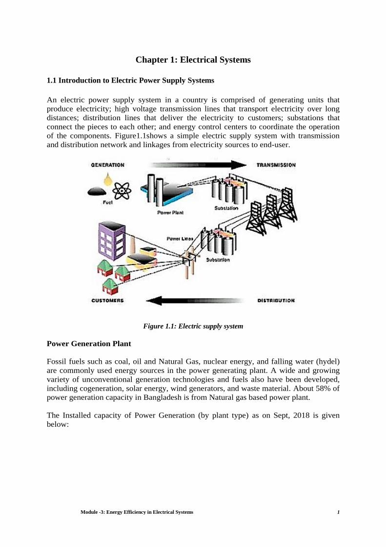
An electric power supply system in a country is comprised of generating units that
produce electricity; high voltage transmission lines that transport electricity over long
distances; distribution lines that deliver the electricity to customers; substations that
connect the pieces to each other; and energy control centers to coordinate the operation
of the components. Figure1.1shows a simple electric supply system with transmission
and distribution network and linkages from electricity sources to end-user.
Figure 1.1: Electric supply system
Power Generation Plant
Fossil fuels such as coal, oil and Natural Gas, nuclear energy, and falling water (hydel)
are commonly used energy sources in the power generating plant. A wide and growing
variety of unconventional generation technologies and fuels also have been developed,
including cogeneration, solar energy, wind generators, and waste material. About 58% of
power generation capacity in Bangladesh is from Natural gas based power plant.
The Installed capacity of Power Generation (by plant type) as on Sept, 2018 is given
below:

Module -3: Energy Efficiency in Electrical Systems 2
Plant Type Installed Capacity (MW)
Power Import 1160
Solar PV 3
Hydro 230
Steam Turbine 2404
Combined Cycle (CC) 5871
Gas Turbine (GT) 1322
Reciprocating Engine (RE) 6053
Total* 17043
*Including Captive Power & Renewable Energy Total Installed Capacity (17,043 +
2,800+290) = 20,133 MW
Figure 1.2 a: Primary Grid System in Bangladesh
Figure 1.2 b: Primary Grid System in Bangladesh
The peak demand is expected to be about 17,304 MW in FY2020 and 25,199 MW in
2025 and 33,708 MW in 2030 based on 7% GDP growth rate.

Module -3: Energy Efficiency in Electrical Systems 3
The maximum power station in Bangladesh run via natural gas, some of them are run by
HFO (Heavy fuel oil). Mainly Diesel oil and Furnace oil are used for thermal power
plant.
Transmission and distribution lines
As per Grid Code of Bangladesh, allowable range for frequency variation is 49.0 to 51.0
Hz. Power plants typically produce 50 cycle/second (Hertz) alternating-current
(AC)electricity with Terminal voltage of different generators are 11 KV, 11.5 KV and
15.75 KV. The transmission and distribution network include sub-stations, lines and
distribution transformers. At the power plant, the 3-phase voltage is stepped up to a
higher voltage for transmission on cables strung on cross-country towers. High voltage
transmission is used so that smaller, more economical wire sizes can be employed to
carry the lower current and to reduce losses. Sub-stations, containing step-down
transformers, reduce the voltage for distribution to industrial users. The voltage is further
reduced for commercial facilities. Electricity must be generated, as and when it is needed
since electricity cannot be stored virtually in the system here is no difference between a
transmission line and a distribution line except for the voltage level and power handling
capability. Transmission lines are usually capable of transmitting large quantities of
electric energy over great distances. They operate at high voltages.
Figure 1.3 Cross Country Tower
Distribution lines carry limited quantities of power over shorter distances. High voltage
(HV) and extra high voltage (EHV) transmission is the next stage from power plant to
transport A.C. power over long distances at voltages like; 400kV, 230 kV and 132 kV.
These are called as the primary grid system. Where transmission is over 1000KM, high
voltage direct current transmission (HVDC) is also favored to minimize the losses.
Sub-transmission network at 230 kV, 132kVconstitutesthenextlinktowards the end user.
High voltage transmission network that transmits the power to grid substation
transformers to be stepped down at 33 kV, 11 kV and 0.4 kV for delivery to the
consumers of various categories.

Module -3: Energy Efficiency in Electrical Systems 4
Distribution at 11kV/6.6kV/3.3kV constitutes the last link to the consumer, who is
connected directly or through transformers depending upon the drawl level of service.
Voltage drop in the line is in relation to the resistance and reactance of line, length and
the current drawn. For the same quantity of power handled, lower the voltage, higher the
current drawn and higher the voltage drop. The current drawn is inversely proportional to
the voltage level for the same quantity of power handled.
The power loss in line is proportional to resistance and square of current. (i.e.,
PLoss=I2R). Higher voltage transmission and distribution thus would help to minimize
line voltage drop in the ratio of voltages, and the line power loss in the ratio of square of
voltages. For instance, if distribution of power is raised from 11 kV to 33 kV, the voltage
drop would be lower by a factor 1/3 and the line loss would be lower by a factor (1/3)2
i.e., 1/9. Lower voltage transmission and distribution also calls for larger quantity of
conductor on account of current handling capacity needed.

Module -3: Energy Efficiency in Electrical Systems 5
Figure 1.4: Primary Grid System in Bangladesh (Source: PGCB)

Module -3: Energy Efficiency in Electrical Systems 6
Cascade Efficiency
The primary function of transmission and distribution equipment is to transfer power
economically and reliably from one location to another. Conductors in the form of wires
and cables strung on towers and poles carry the high-voltage, AC electric current. A
large number of copper or aluminum conductors are used to form the transmission path.
The resistance of the long-distance transmission conductors is to be minimized. Energy
loss in transmission lines is wasted in the form of I2R losses.
Capacitors are used to correct power factor by causing the current to lead the voltage.
When the AC currents are kept in phase with the voltage, operating efficiency of the
system is maintained at a high level.
Circuit-interrupting devices are switches, relays, circuit breakers, and fuses. Each of
these devices is designed to carry and interrupt certain levels of current. Making and
breaking the current carrying conductors in the transmission path with a minimum of
arcing is one of the most important characteristics of this device. Relays sense abnormal
voltages, currents, and frequency and operate to protect the system.
Transformers are placed at strategic locations throughout the system to minimize power
losses in the T&D system. They are used to change the voltage level from low-to-high in
step-up transformers and from high-to-low in step-down units. Since the power loss of a
transmission line is based on I2R, losses can be reduced by stepping up the source
voltage to a high value to proportionally reduce the source current.
The power source to end user energy efficiency link is a key factor
which influences the energy input at the source of supply, consider the
electricity flow from generation to the user in terms of cascade energy
efficiency.
A typical cascade efficiency profile from Generation to 11-33 kV user
industry is illustrated below:
Weighted efficiency for various mix of power generation sources viz.
(Combined Cycle, Reciprocating Engine, Steam turbine and Gas
Turbine) ranges 40-45 % w.r.t. size plant, vintage of plant and
capacity utilization.
Step-up to 400 kV to enable EHV transmission. Envisaged maximum
losses 1.0 % or efficiency of 99%
EHV transmission and substations at 400 kV / 800 kV. Envisaged
maximum losses 1.0 % or efficiency of 99 %
HV transmission & Substations for 132/ 220/ 400 kV. Envisaged
maximum losses 2.5 % or efficiency of 97.5%
Sub-transmission at 66 / 132 kV Envisaged maximum losses 4% or
efficiency of 96%

Module -3: Energy Efficiency in Electrical Systems 7
Step-down to a level of 11 / 33kV. Envisaged losses 0.5% or efficiency of 99.5%
Distribution is finally link to end user at 11 / 33 kV. Envisaged losses maximum 5 % of
efficiency of 95 %
Cascade efficiency from Generation to end user = η1 × η2 × η3 × η4 × η5 × η6 × η7
The cascade efficiency in the T&D system from output of the power plant to the end use
is 87% (i.e. 0.995 x 0.99 x 0.975 x 0.96 x 0.995 x 0.95 = 87%)
Industrial End User
At the industrial end user premises again the plant network elements like transformers at
receiving sub-station, switch gear, lines and cables, load-break switches, capacitors cause
losses which affect the input received energy.
A typical plant single line diagram of electrical distribution system is shown in Figure1.5
Figure 1.5: Electrical Distribution System – Single Line Diagram
The likely network elements that are encountered at industry up to the motor, i.e., pre-
motor system can include:
Outdoor circuit breakers with typical full load losses of 0.002 – 0.015%
Receiving transformers with typical operating efficiency of 99 % or above.
Medium voltage switch gear 5.15kVwhere maximum full load losses can be
between 0.005 - 0.02%
Load break switches where maximum of full load losses can be between 0.003–
0.025 %.
Current limiting reactors can have a maximum full load losses ranging from
0.09% to 0.3 %.

Module -3: Energy Efficiency in Electrical Systems 8
Medium voltage starters can have a maximum full load losses of 0.02% to
0.15%.
Lines and cables can have a maximum loss ranging for 1% to 6% depending
upon lengths, voltage levels, power factor, condition of network in plant
Motor control centers can have a full load losses range from 0.01% to 0.4 %.
Low voltage switchgear can have a full load loss ranging from 0.13 % to 0.34 %.
Thus, as per the links available in the in-plant distribution network, the cascade
efficiency of pre-motor system can be computed, as a product of efficiencies of the
actual links in cascade.
When problems like low voltage at motor terminals are encountered, this pre-motor
system needs to be looked into, for improvement opportunities like;
Relocating transformers close to load centers.
Increasing cable / line size addition of parallel cable, and minimizing jumpers /
loose connections and optimizing line lengths etc.
Tap changing as needed at the transformers.
Capacitor relocation close to load centers or motor terminals, as discussed later.
Adopting best practices like infrared thermograph of distribution network, for
identifying hotspots, which indicate potential are as of break-down/overloading
etc., for attention / maintenance.
ONE Unit saved = TWO Units Generated
After power generation at the plant, it is transmitted and distributed over a wide network.
The standard technical losses are around 9.5% in Bangladesh (Efficiency=90.5%). But
overall T & D (Transmission and Distribution Loss) losses range from 9 –17%. All these
may not constitute technical losses, since un-metered and pilferage are also accounted in
this loss.
When the power reaches the industry, it is received by the transformer. The energy
efficiency of the transformer is generally very high. Next it goes to the motor through
internal plant distribution network. A typical distribution network efficiency including
transformer is 95% and motor efficiency is about 90%. Another 30% (Efficiency=70%)
is lost in the mechanical system which includes coupling / drive train, a driven
equipment such as pump and flow control valves/throttling etc. Thus the overall energy
efficiency becomes 50%. (0.90 x 0.95 x 0.9 x 0.70 = 0.54, i.e., 54% efficiency)
Hence one unit saved in the end user is equivalent to two units generated in the power
plant. (1 Unit /0.5 Eff =2 Units)
1.2 Electricity billing
The electricity billing by utilities for medium & large industries and enterprises
(Category - F to Category – H) is often done on two-part tariff structure, i.e. one part for
capacity (or demand) drawn and the second part for actual energy drawn during the
billing cycle. Capacity or demand is in kW. The reactive energy (i.e.) KVARh drawn by
the customer / service is also recorded and billed for in some utilities, because this would

Module -3: Energy Efficiency in Electrical Systems 9
affect the load on the utility. Accordingly, utility charges for maximum demand, active
energy and reactive power drawn as reflected by the power factor in their billing
structure. In addition, other fixed and variable expenses are also levied.
The tariff structure generally includes the following components:
a) Maximum demand Charges
b) These relate to maximum demand registered during month / billing period and
corresponding rate of utility.
c) Energy Charges
d) These relate to energy (kilo watt hours) consumed during month /billing period
and corresponding rates, often levied in slabs of use rates. Some utilities now
charge on the basis of apparent energy (kVAh), which is a vector sum of kWh
and KVARh.
e) Power factor penalty or bonus rates, as levied by most utilities, are to contain
reactive power drawn from grid.
f) Fuel cost adjustment charges as levied by some utilities are to adjust the
increasing fuel expenses over a base reference value.
g) Electricity duty charges levied w.r.t units consumed.
h) Meter rentals
i) Lighting and fan power consumption is often at higher rates, levied sometimes
on slab basis or on actual metering basis.
j) Interruptible and adjustable rates like night tariff concessions and time of use
rates are also prevalent in tariff concessions and time of use rates are also
prevalent in tariff structure provisions of some utilities.
“Analysis of utility bill data and trending of the same helps energy manager to identify
ways for electricity bill reduction through available provisions in tariff framework, apart
from budgeting”.
The utility employs a tri vector meter of electromagnetic or the state of the art static
electronic tri vector meter, for billing purposes. As apparent, active and reactive energy
are vectorial in nature, the monitoring meter is called Tri vector meter. The minimum
outputs from the electromagnetic meters are:
Maximum demand registered during the month, which is measured in preset
time intervals (say of 30 minute duration) and this is reset at the end of every
billing cycle.
Maximum demand (MD) in kW shall be registered using the technique of
cumulating on integration period controlled by built-in process and the MD shall
be continuously recorded and the highest shall be indicated. (Integration period:
thirty minutes)
Active energy in KWH during billing cycle
Average PF for billing period.
Reactive energy in KVARH during billing cycle and
Apparent energy in KVAH during billing cycle
It is important to note that while maximum demand is recorded, it is not the
instantaneous demand drawn, as is often misunderstood, but the time integrated demand
over the predefined recording cycle.

Module -3: Energy Efficiency in Electrical Systems 10
As example, in an industry, if the drawl over a recording cycle of 30 minutes is:
2500 KW for 4 minutes
3600 KW for 12 minutes
4100 KW for 6 minutes
3800 KW for 8 minutes
The MD recorder will be computing MD as:
(2500x4) + (3600 x 12) + (4100 x 6) + (3800 x 8)
30= 3606. 7kW
The month’s maximum demand will be the highest among such demand values recorded
over the month. The meter registers only if the value exceeds the previous maximum
demand value and thus, even if, average maximum demand is low, the industry/facility
has to pay for the maximum demand charges for the highest value registered during the
month, even if it is occurs for just one recording cycle duration i.e., 30 minutes during
whole of the month (1440 such intervals in a month).
The LCD electronic tri-vector meters have some excellent provisions that can help the
utility as well as the industry. These provisions include:
Substantial memory for logging and recording all relevant events
High accuracy of 0.2 class
Amenability to time of use tariffs
Tamper detection /recording
Measurement of harmonics and Total Harmonic Distortion (THD)
Long service life due to absence of moving parts
Amenability for remote data access/downloads
Analysis and trending of purchased electricity for the past 12 months in a year and cost
components can help the industry to identify key areas such as a voiding power factor
penalty, contract demand reduction and availing time of the tariff advantages etc. for bill
reduction within the utility tariff available framework.
Compiling monthly electricity use data, including all sources like; cogeneration, captive
diesel power generation; doing cost comparison by source, linking power consumption to
production by specific power consumption assessment, would serve as a powerful
information tool for energy manager / auditor to optimize electricity costs for the
industry or facility.
1.3 Electrical load management and maximum demand control
Need for Electrical load management
1. In a macro perspective, the growth in the electricity use and diversity of end use
segments in time of use has led to shortfalls in capacity to meet demand. As
capacity addition is costly and only a long time prospect, better load

Module -3: Energy Efficiency in Electrical Systems 11
management at user end helps to minimize peak demands on the utility
infrastructure as well as better utilization of plant capacities.
2. The utilities use power tariff structure to influence end user in better load
management through measures like time of use tariffs, penalties on exceeding
allowed maximum demand, night tariff concessions etc. Load management is a
powerful means of efficiency improvement both for end user as well as utility.
3. As the demand charges constitute a considerable portion of the electricity bill,
from user angle too there is a need for integrated load management to effectively
control the maximum demand.
Step By Step Approach for Maximum Demand Control
1. Load Curve Generation
Presenting the load demand of a consumer against time of the day is known as a ‘load
curve’. If it is plotted for the 24 hours of a single day, it is known as an ‘hourly load
curve’ and if daily demands plotted over a month, it is called daily load curves. These
types of curves are useful in predicting patterns of drawl, peaks and valleys and energy
use trend in a section or in an industry or in a distribution network as the case may be.
The load factor can also be defined as the ratio of the energy consumed during a given
period to the energy, which would have been used if the maximum demand had been
maintained throughout that period.
Load Factor = (Energy Consumed in 24 Hours) / (Maximum Load Recorded × 24
Hours).
2. Rescheduling of Loads
Rescheduling of large electric loads and equipment operations, in different shifts can be
planned and implemented to minimize the simultaneous maximum demand. For this
purpose, it is advisable to prepare an operation flow chart and a process chart. Analyzing
these charts and with an integrated approach, it would be possible to reschedule the
operations and running equipment in such away as to reduce the maximum demand and
improve the load factor.
3. Staggering of Motor loads
When running of motors of large capacities are involved, it is advisable to stagger the
running of these motors with a suitable planning (as the process may permit) so as to
minimize the simultaneous maximum demand (depending on the conditions of load)
offered by these motors.
4. Storage of Products/in process material/ process utilities like refrigeration
It is possible to reduce the maximum demand by building up storage capacity of
products/ materials, water, chilled water / hot water using electricity during off peak
periods. Off peak hour operations also help to save energy due to favorable conditions
such as lower ambient temperature etc.

Module -3: Energy Efficiency in Electrical Systems 12
Example 1.1
Ice bank system is used in milk & dairy industry. Ice is made in lean period and used in
peak load period and thus maximum demand is reduced.
Shedding of Non-Essential Loads
When the maximum demand tends to reach preset limit, shedding some of non-essential
loads temporarily can help to reduce it. It is possible to install direct demand monitoring
systems, which will switch off non-essential loads when a preset demand is reached.
Simple systems give an alarm, and the loads are shed manually. Sophisticated
microprocessor controlled systems are also available, which provide a wide variety of
control options like:
Accurate prediction of demand
Graphical display of present load, available load, demand limit
Visual and audible alarm
Automatic load shedding in a predetermined sequence
Automatic restoration of load
Recording and metering
5. Operation of Captive Generation, Diesel Generation Sets and Gas Engines
When Diesel/Gas generation sets are used to supplement the power supplied by the
electric utilities, it is advisable to connect the Diesel or Gas sets for durations when
demand reaches the peak value. This would reduce the load demand to a considerable
extent and minimize the demand charges.
6. Reactive Power Compensation
The maximum demand can also be reduced at the plant level by using capacitor banks
and maintaining the optimum power factor. Capacitor banks are available with
microprocessor based control systems. These systems switch on and off the capacitor
banks to maintain the desired Power factor of system and optimize maximum demand
thereby.
1.4 Power factor improvement and benefits
Power factor Basics
In all industrial electrical distribution systems, the pre dominant loads are resistive and
inductive. Resistive loads are incandescent lighting and resistance heating. In case of
pure resistive loads, the voltage (V), current (I), resistance (R) relations are linearly
related, i.e.
V = I × R and kW = V × I
Inductive loads are A.C. Motors, induction furnaces, transformers and ballast-type
lighting. Inductive loads require two kinds of power: (1) active (or working) power to
perform the work and (2) reactive power to create and maintain electro-magnetic fields.
The vector sum of the active power and reactive power make up the total (or apparent)
power used. This is the power generated by the Utilities (Distribution companies) for the
user to perform a given amount of work.

Module -3: Energy Efficiency in Electrical Systems 13
Active power is measured in KW (Kilo Watts)
Reactive power is measured in KVAR (Kilo Volt-Amperes Reactive)
Total Power is measured in KVA (Kilo Volts-Amperes)
Figure 1.6: Power factor
The active power (shaft power required or true power required) in kW and the reactive
power required (KVAR) are 900
apart vectorically in a pure inductive circuit i.e.,
reactive power KVAR lagging the active kW. The vector sum of the two is called the
apparent power or kVA, as illustrated above and the kVA reflects the actual electrical
load on distribution system.
The ratio of kW to kVA is called the power factor which is always less than or equal to
unity. Theoretically, when electric utilities supply power, if all loads have unity power
factor, maximum power can be transferred for the same distribution system capacity.
However, as the loads are inductive in nature with the power factor ranging from 0.2 to
0.9, the electrical distribution network is stressed for capacity at low power factors.
Improving Power Factor
The solution to improve the power factor is to add power factor correction capacitors to
the plant power distribution system. They act as reactive power generators, and provide
the needed reactive power to accomplish KW of work. This reduces the amount of
reactive power and thus total power generated by the Utilities (Distribution companies)
Example 1.2
A chemical industry had installed a 1500 KVA transformer. The initial demand of the
plant was 1160 KVA with power factor of 0.70. The % loading of transformer was about
78% (1160/1500=77.3%). To improve the power factor and thereby avoiding the penalty,
the unit had added about 410 KVAR in motor load end. This improved the power factor
to 89%, and reduced the required KVA to 913, which is the vector sum of KW and
KVAR.
After improvement the plant had avoided penalty and the 1500 KVA transformer now
loaded only to 60% of capacity. This will allow the addition of more loads in the future
to be supplied by the transformer.

Module -3: Energy Efficiency in Electrical Systems 14
Figure 1.7a: Power factor before and after Improvement
Figure 1.7b: Increase in the apparent and reactive powers as a function of the load power factor,
holding the real power of the load constant
The advantages of improvement by capacitor addition
a) Reactive component of the network is reduced and also the total current in the
system from the source end.
b) I2R power losses are reduced in the system because of reduction in current.
c) Voltage level at the load end is increased.
d) KVA loading on the source generators as also on the transformers and lines up to
the capacitors reduces giving capacity relief. A high power factor can help in
utilizing the full capacity of the electrical system.
Cost benefits of PF improvement
While costs of PF improvement are in terms of investment needs for capacitor addition
the benefits to be quantified for feasibility analysis are:
a) Reduced KVA (Maximum demand) charges in utility bill
b) Reduced distribution losses (KWH) within the plant network
c) Better voltage at motor terminals and improved performance of motors
d) A high power factor eliminates penalty charges imposed when operating with a
low power factor
e) Investment on system facilities such as transformers, cables, switchgears etc. for
delivering load is reduced

Module -3: Energy Efficiency in Electrical Systems 15
Selection, Location and Sizing of Capacitor
The figures given in table 1 are the multiplication factors which are to be multiplied with
the input power (kW) to give the KVAR of capacitance required to improve present
power factor to a new desired power factor.
Table 1.1: Multiplication factors for selection of capacitors
Original P.F. Desired P.F.
1.0 0.95 0.90 0.85 0.80
0.55 1.518 1.189 1.034 0.899 0.763 0.60 1.333 1.004 0.849 0.714 0.583 0.65 1.169 0.840 0.685 0.549 0.419 0.70 1.020 0.691 0.536 0.400 0.270
0.75 0.882 0.553 0.398 0.262 0.132 0.80 0.750 0.421 0.266 0.130 0.85 0.484 0.291 0.136 0.90 0.328 0.155
0.95 0.620
Having known the existing power factor, the multiplication factor may be calculated for
raising the power factor from the present value to the desired value.
Example 1.3
If power factor of 30 kW load is to be improved from 0.80 to 0.95, then
Size of the capacitor = kW ×multiplication factor = 30 × 0.421 = 12.63 (or) 13 KVAR
In case of induction motors of different ratings and speeds, in order to improve their
power factor to 0.95 and above, the rating of the capacitor (in KVAR) for direct
connection to induction motor can be referred to in the chapter on electric motors.
Direct relation can also be used for capacitor sizing
KVAR Rating = KW [Tan φ1 – tanφ2]
where, KVAR rating is the size of the capacitor needed, KW is the average power drawn,
tan φ1is the trigonometric ratio for the present power factor, and tanφ2 is the
trigonometric ratio for the desired PF.
φ1 = Existing (Cos-1
PF1) and φ2 = Improved (Cos-1
PF2)
Location of Capacitors
Location of capacitors is an important factor to be considered. For the benefit of
electricity boards, connection of capacitors on H.T. side is good enough. Although the
cost of H.T. capacitor per KVAR is low, the cost of the associated switchgear is quite
high.
Alternatively, the capacitors can be connected on L.T. side of the main substation. The
capacitors may be placed at load centers viz., directly with motors or group of motors at
motor control centers. Correction of PF at the motors has number of advantages, as the

Module -3: Energy Efficiency in Electrical Systems 16
induction motors are the main source of reactive currents in every industrial plant. The
advantages include the absence of additional switchgear; no separate control of capacitor
is required in switching on and off operations and reduced effect of motor inrush
currents.
From energy efficiency point of view, capacitor location at receiving substation only
helps the utility in loss reduction. Locating capacitors at user end motors will help to
reduce loss reduction within the plants distribution network as well and directly benefit
the user by reduced demand cost. Reduction in the distribution loss in KWH when tail
end power factor is raised from PF1 to a new power factor PF2, will be proportional to
[1 - (PF1 / PF2)2]
Figure 1.8: Effect of Location
Capacitors for other loads
The other types of load requiring capacitor application include induction furnaces,
induction heaters, arc welding transformers etc. The capacitors are normally supplied
with control gear for the application of induction furnaces and induction heating
furnaces. The P.F of arc furnaces experiences a wide variation over melting cycle as it
changes from 0.7 at starting to 0.9 at the end of the cycle.
Power factor for arc welders and resistance’s welders is corrected by connecting
capacitors across the primary winding of the transformers, as the normal PF would be in
the range of 0.35. There commended capacitor ratings for various sizes of welding
transformers are given in table below.
Welding Transformer Rating kVA Capacitor Rating KVAR
Single Phase
9 4
12 6
18 8
24 12
30 18

Module -3: Energy Efficiency in Electrical Systems 17
Three Phase
57 16.5
95 30
128 45
160 60
Performance assessment of power factor capacitors
Voltage effects: Ideally capacitor voltage rating is to match the supply voltage. If the
supply voltage is lower, the reactive KVAR produced will be the ratio V12/V2
2 where V1
is the actual supply voltage, V2 is the rated voltage.
On the other hand, if the supply voltage exceeds rated voltage, the life of the capacitor is
adversely affected.
Table 1.2: Effect of addition of KVAR capacitor
KVAR
Added
Phase
Voltage Phase Current
Total
(kW)
Total
(kVA)
Power
Factor
0 269 121 69 96 0.72
15 268 109 69 84 0.8
30 270 100 70 80 0.87
45 271 92 70 74 0.94
60 272 88 70 71 0.98
75 273 87 70 70 0.99
90 274 89 70 73 0.95 (1.05)
105 276 95 70 79 0.89 (1.11)
Material of capacitors: Power factor capacitors are available in various types by
dielectric material used as; paper/poly propylene etc. The watt loss per KVAR as well as
life vary with respect to the choice of the dielectric material and hence is a factor to be
considered while selection.
Connections: Shunt capacity or connections are adopted for almost all industry/end user
applications, while series capacitors are adopted for voltage boosting in distribution
networks.
Operational performance of capacitors: This can be made by monitoring capacitor
charging current vis- a- vis the rated charging current. Capacity of fused elements can be
replenished as per requirements. Portable analyzers can be used for measuring KVAR
delivered as well as charging current.
Some checks that need to be adopted in use of capacitors are:
i. Name plates can be misleading with respect to ratings. It is good to check by
charging currents.
ii. Capacitors boxes may contain only insulated compound and insulated terminals
with no capacitor elements inside.

Module -3: Energy Efficiency in Electrical Systems 18
iii. Capacitors for single phase motor starting and those used for lighting circuits for
voltage boost, are not power factor capacitor units and these cannot with stand
power system conditions.
iv. Transformers
A transformer can accept energy at one voltage and deliver it at another voltage. This
permits electrical energy to be generated at relatively low voltages and transmitted at
high voltages and low currents, thus reducing line losses.
Transformers consist of two or more coils that are electrically insulated, but magnetically
linked. The primary coil is connected to the powers our and the secondary coil connects
to the load. The turn’s ratio is the ratio between the number of turns on the primary to the
turns on the secondary.
The secondary voltage is equal to the primary voltage times the turn’s ratio. Ampere-
turns are calculated by multiplying the current in the coil times the number of turns.
Primary ampere-turns are equal to secondary ampere-turns. Voltage regulation of a
transformer is the percent increase in voltage from full load to no load.
Types of Transformers
Transformers are classified as two categories as given below:
Power transformers: It is used in transmission network of higher voltages, deployed for
step-up and step down transformer application. (400 kV, 200 kV, 110kV, 66kV, 33kV)
Distribution transformers: It is used for lower voltage distribution networks as a means to
end user connectivity. (11.kV, 6.6kV, 3.3kV, 440V, 230V)
Rating of transformer
Rating of the transformer is calculated based on the connected load and applying the
diversity factor on the connected load, applicable to the particular industry and arrive at
the KVA rating of the Transformer. Diversity factor is defined as the ratio of overall
maximum demand of the plant to the sum of individual maximum demand of various
equipment. Diversity factor varies from industry to industry and depends on various
factors such as individual loads, load factor and future expansion needs of the plant.
Diversity factor will always be less than one.
Location of transformer
Location of the transformer is very important as far as distribution loss is concerned.
Transformer receives HT voltage from the grid and steps it down to the required voltage.
Transformers should be placed close to the load centre, considering other features like
optimization needs for centralized control, operational flexibility etc. This will bring
down the distribution loss in cables.
Transformer Losses and Efficiency
The efficiency varies anywhere between 96 to 99 percent. The efficiency of the
transformers not only depends on the design but also on the effective operating load.

Module -3: Energy Efficiency in Electrical Systems 19
Transformer losses consist of two parts.
No-load loss (also called core loss) is the power consumed to sustain the magnetic field
in the transformer's steel core. Core losses are caused by two factors: hysteresis is and
eddy current losses. Hysteresis is loss is that energy lost by reversing the magnetic field
in the core as the magnetizing AC rises and falls and reverses direction. Eddy current
loss is a result of induced currents circulating in the core. Core loss occurs whenever the
transformer is energized; core loss does not vary with load.
Load loss (also called copper loss) is associated with full-load current flow in the
transformer windings. Copper loss is power lost in the primary and secondary windings
of a transformer due to the ohmic resistance of the windings. Copper loss varies with the
square of the load current.(P=I2R).
For a given transformer, the manufacturer can supply values for no-load loss, PNO-
LOAD, and load loss, PLOAD. The total transformer loss, PTOTAL, at any load level
can then be calculated from:
PTOTAL = PNO-LOAD+ (% Load/100)2
x PLOAD
Where transformer loading is known, the actual transformers loss at given load can be
computed as:
Table 1.3: Typical Transformer Loss for Distribution Transformers (DT’s) above 100kVA
KVA Rating Voltage Rating No load loss(W) Load Loss(W) Impedance%
160 425 3000 5
200 570 3300 5
250 620 3700 5
315 800 4600 5
500 11000/433 1100 6500 5
630 1200 7500 5
1000 1800 11000 5
1600 2400 15500 5
2000 3000 20000 6
630 1450 7500 5
1000 33000/433 2200 11500 5
1600 3000 16000 6.25
2000 3500 21000 6.25
Voltage fluctuation control
A control of voltage in a transformer is important due to frequent changes in supply
voltage level. Whenever the supply voltage is less than the optimal value, there is a
chance of nuisance tripping of voltage sensitive devices. The voltage regulation in

Module -3: Energy Efficiency in Electrical Systems 20
transformers is done by altering the voltage transformation ratio with the help of tapping.
There are two methods of tap changing facility available.
Off-circuit tap changer
It is a device fitted in the transformer, which is used to vary the voltage transformation
ratio. Here the voltage levels can be varied only after isolating the primary voltage of the
transformer.
On load tap changer (OLTC)
The voltage levels can be varied without isolating the connected load to the transformer.
To minimise the magnetization losses and to reduce the nuisance tripping of the plant,
the main transformer (the transformer that receives supply from the grid) should be
provided with On Load Tap Changing facility at design stage. The downstream
distribution transformers can be provided with off-circuit tap changer.
The On-load gear can be put in auto mode or manually depending on the requirement.
OLTC can be arranged for transformers of size 250kVA onwards. However, the
necessity of OLTC below 1000 kVA can be considered after calculating the cost
economics.
Parallel operation of transformers
The design of Power Control Centre (PCC) and Motor Control Centre (MCC) of any
new plant should have the provision of operating two or more transformers in parallel.
Additional switch gears and bus couplers should be provided at design stage.
Whenever two transformers are operating in parallel, both should be technically identical
in all aspects and more importantly with same impedance level. This will minimise the
circulating current between transformers.
Where the load is fluctuating in nature, it is preferable to have more than one transformer
running in parallel, so that the load can be optimized by sharing the load between
transformers. The transformers can be operated close to the maximum efficiency range
by this operation.
Energy Efficient Transformers
Most energy loss in dry-type transformers occurs through heat or vibration from the core.
The new high-efficiency transformers minimize these losses. The conventional
transformer is made up of a silicon alloyed iron (grain oriented) core. The iron loss of
any transformer depends on the type of core used in the transformer. The latest
technology is to use for the amorphous core. Amorphous material has great advantage in
reducing No load loss.
Amorphous core material (AM) offers both reduced hysteresis loss and eddy current loss
because this material has a random grain and magnetic domain structure which results in
high permeability giving a narrow hysteresis curve compared to conventional core
material. Eddy current losses are reduced by the high resistivity of the amorphous
material, and the reduced thickness of the film (thickness is approximately 0.03 mm,

Module -3: Energy Efficiency in Electrical Systems 21
which is about 1/10 comparing with silicon steel). Amorphous core transformers offer a
70 to 80% reduction in no-load losses compared to transformers using conventional core
material.
Figure 1.9: Comparison of Conventional and Amorphous Core Transformers
Example 1.4
Transformer loss calculation
An engineering industry has installed three numbers of 1000KVA transformers for an
electrical load of 1500KVA. The No-load loss and the full load loss of the transformers
were collected from the transformer certificates as 2.8KW and 11.88KW respectively.
Estimate the total loss when 3 transformers in parallel operation and also 2 transformers
parallel operation. The transformer losses can also be obtained from manufacturers test
certificate which are available in the plant.
a) Total loss when Two transformers in parallel operation:
No load loss = 2 x 2.8 =5.6
Load Loss = 2 x (750/1000)^2 x 11.88
Total Loss = 5.6 + 13.36 =18.96
b) Total loss when Three transformers in parallel operation: No load loss = 3 x 2.8 =
8.4KW
Load loss = 3 x (500/1000)^2 x 11.88 = 8.91 kW
Total loss = 17.31 kW
Savings by operating 3 transformers in parallel
= 18.96-17.31= 1.65 kWh
= 1.65kwh x 24Hrs x 365 days = 14454 kWh /year
1.5 System distribution losses
In an electrical system often the constant no load losses and the variable load losses are
to be assessed alongside, over long reference duration, towards energy loss estimation.
Identifying and calculating the sum of the individual contributing loss components is a
challenging one, requiring extensive experience and knowledge of all the factors
impacting the operating efficiencies of each of these components.

Module -3: Energy Efficiency in Electrical Systems 22
For example the cable losses in any industrial plant will be of the order of 2 to 4 percent.
Note that all of these are current dependent, and can be readily mitigated by any
technique that reduces facility current load.
In system distribution loss optimization, the various options available include:
Relocating transformers and sub-stations near to load centers
Re-routing and re-conducting such feeders and lines where the losses/voltage
drops are higher.
Power factor improvement by incorporating capacitors at load end.
Optimum loading of transformers in the system.
Opting for lower resistance All Aluminum Alloy Conductors (AAAC) in place of
conventional Aluminum Cored Steel Reinforced (ACSR) lines
Minimizing losses due to weak links in distribution network such as jumpers,
loose contacts, old brittle conductors.
Distribution loss assessment and optimization studies today are feasible on
account of accurate metering developments on the one hand and availability of
powerful computer based load flow analysis packages on the other.
Using full infrared thermography system, each electrical panel can be scanned to
identify points of high system heat. Called “hotspots”, these high heat points
result from connections become looser corroded overtime. The resulting increase
in resistance at that’s pot in the system can add wattage losses to the electrical
energy consumption. These hot spots also create safety risks and risks to abrupt
system failure. Fixing them is often as simple as de-energizing that point in the
system, and then using a wrench to tighten a bolt.
As far as electricity distribution utilities are concerned, involving large network and
complex connectivity features, there exist well proven computer based application
packages which can be used for network load flow analysis. The analysis outputs can
help a utility engineer to assess the extent of transmission and distribution losses, to
identify sections for improvement where voltage drops are high, to identify avenues for
loss reduction such as ideal location of sub-stations, feeder augmentation, etc.
1.6 Harmonics and its Effects
In any alternating current network, flow of current depends upon the voltage applied and
the impedance (resistance to AC) provided by elements like resistances, reactance of
inductive and capacitive nature. As the value of impedance in above devices is constant,
they are called linear whereby the voltage and current relation is of linear nature.
Example for Linear loads
Linear loads occur when the impedance is constant; then the current is proportional to the
voltage (A straight – line graph, as shown in Figure–1.10). Simple loads, composed of
one of the elements shown in Figure–1.10, do not produce harmonics.

Module -3: Energy Efficiency in Electrical Systems 23
Figure 1.10: Linearloads
However in real life situation, various devices liked diodes, silicon controlled rectifiers,
thyristors, voltage & current controllers, induction & arc furnaces are also deployed for
various requirements and due to their varying impedance characteristic, these Non-
Linear devices cause distortion in voltage and current waveforms which is of increasing
concern in recent times.
Example for Non-Linear loads
Non-linear loads occur when the impedance is not constant; then the current is not
proportional to the voltage (as shown in Figure 1.11. Combinations of the components
shown in Figure 1.11 normally create non-linear loads and harmonics.
Figure 1.11: Non-Linear loads
Harmonics occurs as spikes at intervals which are multiples of the mains (supply)
frequency and these distort the pure sine wave form of the supply voltage ¤t. Thus
harmonics are multiples of the fundamental frequency of an electrical power system. If
for example, the fundamental frequency is 50Hz, then the 5th harmonic is five times that
frequency, or 250 Hz. Likewise, the 7th harmonic is seven times the fundamental or
350Hz, and so on for higher order harmonics.
The magnitude and order of harmonics is governed by the nature of the device being
used and the impact is expressed as Total Harmonic Distortion (THD). Harmonics can be
expressed in terms of current or voltage

Module -3: Energy Efficiency in Electrical Systems 24
In terms of voltage it is expressed as a percentage of fundamental voltage by the
expression
where V1 is the fundamental frequency voltage and Vn is nth
harmonic voltage
component.
In terms of current it is expressed as below
A 5th harmonic current is simply a current flow in gat 250Hz on a 50Hz system. The 5th
harmonic current flowing through the system impedance creates a 5th harmonic voltage.
The following is the formula for calculating the THD for current:
I1 = current at 50 Hz = 250 Amps, I5 = current at 250 Hz = 50 Amps I7 = current at 350
Hz = 35 Amps
If I1 = 250 Amps, I5 = 50 Amps and I7 = 35Amps
When harmonic currents flow in a power system, they are known as poor “power
quality”. Other causes of poor power quality include transients such as voltages pikes,
surges, sags, and ringing. Because they repeat every cycle, harmonics are regarded as a
steady-state cause of poor power quality.
The harmonic assessment can be carried out at site by using a load analyzer. The wave
form is sampled and analyzers cans through various harmonic frequencies, i.e. multiples
of the mains frequency for assessing THD. Load analysers are available in market, which
can measure THD up to 63rd harmonic.
Causes and Effects of Harmonics in electrical systems
Devices that draw non-sinusoidal currents when a sinusoidal voltage is applied create
harmonics. Frequently these are devices that convert AC to DC. Listed below are some
of these devices.
Electronic Switching Power Converters
Computers, Uninterruptible power supplies (UPS), Solid-state rectifiers
Electronic process control equipment, PLC’s, etc.
Electronic lighting ballasts, including light dimmer
Reduced voltage motor controllers

Module -3: Energy Efficiency in Electrical Systems 25
Arcing Devices
Discharge lighting, e.g. Fluorescent, Sodium and Mercury vapor
Arc furnaces, Welding equipment, Electrical traction system
Ferromagnetic Devices
Transformers operating near saturation level
Magnetic ballasts (Saturated Iron core)
Induction heating equipment, Chokes, Motors
Appliances
TV sets, air conditioners, washing machines, microwave ovens
Fax machines, photocopiers, printers
These devices use power electronics liked diodes and thyristors which area growing
percentage of the load in industrial power systems. Normally each load would manifest a
specific harmonic spectrum. Many problems can arise from harmonic currents in a power
system. Some problems are easy to detect. Higher RMS current and voltage in the system
are caused by harmonic currents, which can result in any of the problems listed below.
Effects of Harmonics on Network
The effects of harmonics on distribution network include:
Metering errors in electromagnetic type meters.
Overloading and overheating of motors due to increased iron losses &
overheating of conductors.
Overloading of neutral conductor especially in low voltage distribution network
and High neutral currents
Malfunctioning of control equipment and protection relays due to false signals.
Blown Fuses (no apparent fault)
Misfiring of AC and DC Drives
Tripped Circuit Breakers Voltage distortion
High neutral to ground voltages Increased system losses (heat)
Rotating and electronic equipment failures
Capacitor bank over-load and failures
Reduced power factor
Source Typical Harmonics
6 Pulse Drive/Rectifier 5,7,11,13,17,19…
12 Pulse Drive/Rectifier 11,13,23,25…
18 Pulse Drive 17,19,35,37…
Switch-Mode Power Supply 3,5,7,9,11,13…
Fluorescent Lights 3,5,7,9,11,13…
Arcing Devices 2,3,4,5,7...
Transformer Energization 2,3,4
Module -3: Energy Efficiency in Electrical Systems 26
Generally, the magnitude decreases as harmonic order increases.
h = np +/-1
h = order of harmonics, n = an integer 1, 2, 3,…., p = number of pulses per cycle
For a three phase bridge rectifier, since the number of pulses p = 6 per line frequency
cycle, the characteristic or dominant harmonics are: h = n ⋅6 ± 1 = 5, 7, 11, 13, 17, 19,
23, 25, 35, 37…
Harmonic Filters
Harmonic filters consist of a capacitor bank and reactor in series are designed and
adopted for suppressing harmonics, by providing low impedance path for harmonic
component. The Harmonic filters connected suitably near the equipment generating
harmonics help to reduce THD to acceptable limits. In present context where no Electro
Magnetic Compatibility regulations exist, an application of Harmonic filters is very
relevant for industries having diesel power generation sets and co-generation units.
Energy managers / auditors can address the issue of harmonics from the point of view of
energy efficiency and power quality assurance.
The Harmonic Mitigation solutions currently in use in the industry broadly fall into the
following categories:
1. Passive Harmonic Filter (PHF)
2. Advance Active Filters (AAF)
3. Active Front End based VFDs (AFE)
Passive Harmonic Filter (PHF)
It is the most common method for the cancellation of harmonic current in the distributed
system. These filters are basically designed on principle either single tuned/double tuned
or band pass filter technology. Passive filters (Figure 1.20) offer very low impedance in
the network at the tuned frequency to divert all the harmonic current at the tuned
frequency.
Advance Active Filters (AAF)
It is connected parallel with the distribution system. Distribution system consists of a
wide percentage of harmonics produced by non- linear loads. Active filters (Figure 1.21)
compensate current harmonics by injecting equal magnitude but opposite phase harmonic
compensating current.
Active Front End based VFDs (AFE)
It is used in VFDs has the major advantage of mitigation of harmonics without using
external filter, to maintain unity power factor at the point of common coupling,
Bidirectional power flow makes recovery of energy to the mains by saving it, Clean
power to the grid which in turn does not affect the other loads connected to it,
maintaining the DC voltage irrespective of the supply variations.

Module -3: Energy Efficiency in Electrical Systems 27
Harmonics Limits:
The permissible harmonic limit for different current (Isc / IL) as per IEEE standard is
given in Table 1.4 and for different bus voltage are given in Table 1.5 Current Distortion
Limits for General Distribution System’s end-User limits (120 Volts To 69,000 Volts)
Table 1.4 Maximum Harmonic Current Distortion in % of IL
Individual Harmonic Order (Odd Harmonics)
Isc/IL h<11 11 ≤ h < 17 17 ≤ h < 23 23 ≤ h < 35 35 ≤ h TDD
< 20* 4.0 2.0 1.5 0.6 0.3 5.0
20 < 50 7.0 3.5 2.5 1.0 0.5 8.0
50 < 100 10.0 4.5 4.0 1.5 0.7 12.0
100 < 1000 12.0 5.5 5.0 2.0 1.0 15.0
> 1000 15.0 7.0 6.0 2.5 1.4 20.0
Even harmonics are limited to 25% of the odd current harmonic limits above.
Current distortions that result in a direct current offset, e.g. half wave converters are
not allowed.
*All power generation equipment is limited to these values of current distortion,
regardless of actual Isc/IL.
Where,
Isc = Maximum short circuit current at PCC.
And IL = Maximum Demand Load Current (fundamental frequency component) at
PCC.
TDD = Total demand distortion (RSS), harmonic current distortion in % of maximum
demand load current (15 or 30 min demand).
Table 1.5 Total Harmonic Distribution for Different Voltage Levels in %
Bus Voltage at PCC Individual Voltage
Distortion (%)
Total Voltage
Distortion THD (%)
69 kV and below 3.0 5.0
69.001 kV Thru 161 kV 1.5 2.5
161 kV and above 1.0 1.5
Note:
High voltage systems can have up to 2.0% THD where the cause is an HVDC terminal
that will attenuate by the time it is tapped for a user.
Two very important points must be made in reference to the above.
1. The customer is responsible for maintaining current distortion to within
acceptable levels, while the utility is responsible for limiting voltage distortion.
2. The limits are only applicable at the point of common coupling (PCC) between
the utility and the customer. The PCC, while not explicitly defined, is usually
regarded as the point at which the utility equipment ownership meets the
customer’s or the metering point.

Module -3: Energy Efficiency in Electrical Systems 28
Therefore, the above limits cannot be meaningfully applied to distribution panels or
individual equipment within a plant. The entire plant must be considered complying with
these limits.
1.7 A Glossary of Basic Electrical Terms
V Symbolizes volts or the electromotive force or electric pressure. Symbolizes
the electric current flowing in the circuit in amperes.
I Symbolizes the electric current flowing in the circuit in amperes.
P Power in watts or kilowatts, indicates the real working component of the
energy put in.
KVA
Indicates kilovolt amperes or the apparent power that determines the heating
effect on the AC equipment and systems. All elements of the power systems
must be sized to accommodate this burden.
KVAR Kilovolt amperes reactive, or the ‘Phantom Component’ that vectorally
combines with real power, to determine KVA on electric systems.
PF Power factor or the ratio of real power (KW) to apparent power (KVA)
percentage or as a decimal value.
Φ
Phase angle on the alternating current system, or the measure of the vector
displacement between true power and apparent power, power factor
expressed as the decimal value is the cosine of φ
kWh
Kilowatt-hours are the unit of electrical energy. KWh is obtained by
integrating power, expressed in KW with time. For example, a power of 2KW
appliance for 15 minutes (1/4 hour) indicates an energy consumption of 2 x
1⁄4 = 0.5 kWh.
Power
√3 × V × I × PF
for 3 phase systems, where V = Line voltage, I = line current
• In delta connected electrical system, V line = V phase, I lines = √3 I phase
• In star connected electrical system, V line = √3 V phase, I lines = I phase
and V × I x PF for single phase systems
KVA √3 × V × I for 3 phase systems and V x I for single-phase systems.
Load factor Load factor is the ratio of the average demand (KVA or KW) to the peak
demand for a power system. High load factor leads to better utilization of
installed capacity. Demand
Factor Demand factor is the ratio of maximum demand to the connected load.
Peak
Demand or
Peak Load
The highest demand on an electric utility system is called peak loador Peak
Demand. Demand varies with time every day and also from season to season.
As electricity cannot be stored easily, utilities have to provide the generating
capacity to meet peak demand even it lasts for a short duration.
Connected
Load
Connected load is the summation of nameplate ratings (kW or kVA) of the
electrical equipment installed in a consumer's premises

Module -3: Energy Efficiency in Electrical Systems 29
Load
Management
Load management is a set of techniques for control of power supply and
demand to increase the system load factor. Electric utilities as well as
consumers can reduce the peak (maximum demand) by load shifting or load
shedding (power cuts)
Analysis of Electrical Power Systems
An analysis of an electrical power system may uncover energy waste, fire hazards, and
equipment failure. Facility / Energy managers increasingly find that reliability-centered
maintenance can save money, energy, and downtime.
System Problem Common Causes Possible Effects
Solutions
Voltage
imbalances among
the three phases
Improper transformer tap
settings, single-phase loads
not balanced among phases,
poor connections, bad
conductors, transformer
grounds or faults.
Motor vibration,
premature motor failure
A 5% imbalance causes
a 40% increase
in motor losses.
Balance loads
among phases.
Voltage deviations
from rated voltages
( too low or high)
Improper transformer
settings, Incorrect selection
of motors.
Over-voltages in
motors reduce
efficiency, power factor
and equipment life
Increased temperature
Correct
transformer
settings, motor
ratings and
motor
input voltages
Poor connections in
distribution or at
connected loads.
Loose bus bar connections,
loose cable connections,
corroded connections, poor
crimps, loose or worn
contactors
Produces heat, causes
failure at connection
site, leads to voltage
drops and voltage
imbalances
Use Infra-Red
camera to
locate
hot-spots and
correct.
Undersized
conductors.
Facilities expanding beyond
original designs, poor power
factors
Voltage drop and
energy waste.
Reduce the
load by
conservation
load
scheduling. Insulation leakage
Degradation over time due to
extreme temperatures,
abrasion, moisture,
chemicals
May leak to ground or
to another phase.
Variable energy waste.
Replace
conductors,
insulators
Low Power Factor
Inductive loads such as
motors, transformers, and
lighting ballasts Non-linear
loads, such as most
electronic loads.
Reduces current-
carrying capacity of
wiring, voltage
regulation
effectiveness, and
equipment life.
Add capacitors
to counter act
reactive loads.
Harmonics (non-
sinusoidal voltage
and/or current wave
forms)
Office-electronics, UPSs,
variable frequency drives,
high intensity discharge
lighting and electronic and
core-coil ballasts.
Over-heating of neutral
conductors, motors,
transformers, switch
gear. Voltage drop, low
power factors, reduced
capacity.
Take care with
equipment
election and
isolate
sensitive
electronics
from noisy
circuits.

Module -3: Energy Efficiency in Electrical Systems 30
Chapter 2: Electrical Motors
2.1 Introduction
Electric motors convert electrical power into mechanical power by the interaction
between the magnetic fields set up in the stator and rotor windings within a motor. In
industrial applications, electric motor driven systems are used for various applications
such as pumping, compressed air, fans, conveyors etc.
All industrial electric motors can be broadly classified as Induction Motors, Direct
Current Motors or Synchronous Motors. All motor types have the same four operating
components: Stator (stationary windings), Rotor (rotating windings), Bearings, and
Frame (enclosure). All motors convert electrical energy in to mechanical energy by the
interaction between the magnetic fields set up in the stator and rotor windings.
2.2 Motor Types
2.2.1 Induction Motors
Induction motors are the most commonly used in industrial applications. The induction
motor is the most popular type of ac motor because of its simplicity and ease of
operation. An induction motor does not have a separate field circuit; instead, it depends
on transformer action to induce voltages and currents in its field circuit. In fact, an
induction motor is basically a rotating transformer. Its equivalent circuit is similar to that
of a transformer, except for the effects of varying speed. There are two types of induction
motor rotors, cage rotors and wound rotors. Cage rotors consist of a series of parallel
bars all around the rotor, shorted together at each end. Wound rotors are complete three-
phase rotor windings, with the phases brought out of the rotor through slip rings and
brushes. Wound rotors are more expensive and require more maintenance than cage
rotors, so they are very rarely used (except sometimes for induction generators).
Figure 2.1: Induction Motor
In induction motors, the induced magnetic field of the stat or winding induces a current
in the rotor. In induction machines, rotor currents are induced in the rotor windings by a
combination of the time-variation of the stator currents and the motion of the rotor
relative to the stator. If a 3-phase supply is fed to the stator windings of a 3-phase motor,
a magnetic flux of constant magnitude, rotating at synchronous speed is set up. At this

Module -3: Energy Efficiency in Electrical Systems 31
point, the rotor is stationary. The rotating magnetic flux passes through the air gap
between the stator & rotor and sweeps past the stationary rotor conductors. This rotating
flux, as it sweeps, cuts the rotor conductors, thus causing an e.m.f to be induced in the
rotor conductors. As per the Faraday’s law of electromagnetic induction, it is this relative
motion between the rotating magnetic flux and the stationary rotor conductors, which
induces an e.m.f on the rotor conductors. Since the rotor conductors are shorted and form
a closed circuit, the induced e.m.f produces a rotor current whose direction is given by
Lenz’s Law, is such as to oppose the cause producing it. In this case, the cause which
produces the rotor current is the relative motion between the rotating magnetic flux and
the stationary rotor conductors. Thus to reduce the relative speed, the rotor starts to rotate
in the same direction as that of the rotating flux on the stator windings, trying to catch it
up. The frequency of the induced e.m.f is same as the supply frequency. An induction
motor normally operates at a speed near synchronous speed, but it can never operate at
exactly nsync.
Slip-ring motor
The slip-ring motor or wound-rotor motor is a variation of the squirrel cage induction
motor. While the stator is the same as that of the squirrel cage motor, the rotor of a slip-
ring motor is wound with wire coils. A slip ring induction motor is an asynchronous
motor, as the rotor never runs in synchronous speed with the stator poles. The ends of the
windings are connected to slip rings so that resistors or other circuitry can be inserted in
series with the rotor coils through carbon brushes that slide on the slip-rings allowing an
electrical connection with the rotating coils. This basically is the difference in
construction between a squirrel cage and slip-ring motors. These are helpful in adding
external resistors and contactors. The slip necessary to generate the maximum torque
(pull-out torque) is directly proportional to the rotor resistance. In the slip-ring motor, the
effective rotor resistance is increased by adding external resistance through the slip rings.
Thus, it is possible to get higher slip and hence, the pull-out torque at a lower speed. A
particularly high resistance can result in the pull-out torque occurring at almost zero
speed, providing a very high pull-out torque at a low starting current. As the motor
accelerates, the value of the resistance can be reduced, altering the motor characteristic to
suit the load requirement. Once the motor reaches the base speed, external resistors are
removed from the rotor. This means that now the motor is working as the standard
induction motor.
This motor type is ideal for very high inertia loads, where it is required to generate the
pull-out torque at almost zero speed and accelerate to full speed in the minimum time
with minimum current draw.
Modifying the speed torque curve by altering the rotor resistors, the speed at which the
motor will drive a particular load can be altered. At full load the speed can be reduced
effectively to about 50% of the motor synchronous speed, particularly when driving
variable torque/variable speed loads, such as printing presses, compressors, conveyer
belts, hoists and elevators. Reducing the speed below 50%, results in very low efficiency
due to higher power dissipation in the rotor resistances. This type of motor is used in
applications for driving variable torque/ variable speed loads.

Module -3: Energy Efficiency in Electrical Systems 32
2.2.2 Direct-Current Motors
Direct-Current motors, as then am implies, use direct, i.e. unidirectional, current. Used in
special applications, they only represent small percentage of motors used in industry,
e.g. where high torque starting or where smooth acceleration over a broad speed range is
required. Before the widespread use of power electronic rectifier-inverters, dc motors
were unexcelled in speed control applications.
The working of DC motor is based on the principle
That when a current-carrying conductor is placed in a magnetic field, it experiences a
mechanical force. The direction of mechanical force is given by Fleming’s Left-hand
Rule. There is no basic difference in the construction of a DC generator and a DC motor.
In fact, the same D.C machine can be used interchangeably as a generator or as a motor.
There are five major types of dc motors in general use:
1. The separately excited dc motor
2. The shunt dc motor
3. The permanent-magnet dc motor
4. The series dc motor
5. The compounded dc motor
2.2.3 Synchronous Motors
In synchronous machines, rotor-winding currents are supplied directly from the
stationary frame through a rotating contact. AC power is fed to the stator of the
synchronous motor. The rotor is fed by dc from a separate source. The rotor magnetic
field locks onto the stator rotating magnetic field and rotates at the same speed. The
speed of the rotor is a function of the supply frequency and the number of magnetic poles
in the stator. While induction motors with a slip, i.e., rpm is less than the synchronous
speed, the synchronous motor rotate with no slip, i.e., the rpm is same as the
synchronous speed governed by supply frequency and number of poles. The basic
principle of synchronous motor operation is that the rotor "chases" the rotating stator
magnetic field around in a circle, never quite catching up with it. The slip energy is
provided for by the D.C. excitation power.
2.3 Motor Characteristics
2.3.1 Motor Speed
The speed of a motor is the number of revolutions in a given time frame, typically
revolutions per minute (RPM). The speed of an AC motor depends on the frequency of
the input power and the number of poles for which the motor is wound. The synchronous
speed in RPM is given by the following equation, where the frequency is in hertz or
cycles per second:

Module -3: Energy Efficiency in Electrical Systems 33
Motors have synchronous speeds like 3000 / 1500 / 1000 / 750 / 600 / 500 / 375 rpm
corresponding to no. of poles (always even) being 2, 4, 6, 8, 10, 12, 16 and given the
mains frequency of 50 cycles / sec.
The actual speed with which the motor operates, will be less than the synchronous speed.
The difference between synchronous and full load speed is called slip and is measured in
percent. It is calculated using this equation:
As per relation stated above, the speed of an AC motor is determined by the number of
motor poles and by the input frequency. It can also be seen that theoretically speed of an
AC motor can be varied infinitely by changing the frequency. For practical limits to
speed variation, manufacturer’s guidelines should be referred to. With the addition of a
Variable Frequency Drive (VFD), the speed of the motor can be decreased as well as
increased.
2.3.2 Volts/Hz Relationship
It has been seen that by changing the frequency, one can change the speed of the motor.
However, frequency is not the only parameter that must be changed. Notice in the motor
model below that the impedance of a motor will change with frequency since the
impedance of an inductor equals to 2πfl. At low frequencies, this impedance approaches
zero making the circuit appear to be a short circuit.
Figure 2.2: Volts/Hz Relationship
To maintain a constant flux in the motor, the voltage to the motor must also be changed.
This ratio is constant over most of the entire speed range. By keeping the ratio constant, a
fixed speed induction motor can be made to run at variable speed and provide constant
torque as required by driven machine. At low speeds, due to the motor having inherent
resistance in the windings, the ratio must be altered to provide enough magnetizing flux
to spin the motor. The VFD allows this relationship to be altered by changing the voltage
boost parameter.

Module -3: Energy Efficiency in Electrical Systems 34
Figure 2.3: Efficiency at different load
2.3.3 Power Factor
The power factor of the motor is given as:
Power Factor = Cos φ = kW/kVA
As the load on the motor comes down, the magnitude of the active current reduces.
However, there is no corresponding reduction in the magnetizing current, with the
result that the motor power factor reduces, with a reduction in applied load. Induction
motors, especially those operating below their rated capacity, are the main reason for low
power factor in electric systems.
2.3.4 Motor Efficiency Parameters
Two important attributes relating to efficiency of electricity use by A.C. Induction
motors are efficiency (η), defined as the ratio of the mechanical energy delivered at the
rotating shaft to the electrical energy input at its terminals, and power factor (PF),
defined as the ratio of the real power (kW) to apparent power (kVA) drawn by the motor.
Motors, like other inductive loads, are characterized by power factors less than one. As a
result, the total current draw needed to deliver the same real power is higher than for a
load characterized by a higher PF. An important effect of operating with a PF less than
one is that resistance losses in wiring upstream of the motor will be higher, since these
are proportional to the square of the current. Thus, both a high value for η and a PF close
to unity are desired for efficient overall operation in a plant.
Figure 2.4: Power factor at different loads

Module -3: Energy Efficiency in Electrical Systems 35
Squirrel age motors are normally more efficient than slip-ring motors, and higher-speed
motors are normally more efficient than lower-speed motors. Efficiency is also a
function of motor temperature. Totally-enclosed, fan-cooled (TEFC) motors are more
efficient than screen- protected drip- proof (SPDP) motors. Also, as with most
equipment, motor efficiency increases with the rated capacity.
The efficiency of a motor is determined by intrinsic losses that can be reduced only by
changes in motor design. Intrinsic losses are of two types–fixed, i.e., independent of
motor load, and variable, i.e., dependent on load. Fixed losses consist of magnetic core
losses and friction and wind age losses. Magnetic core losses (sometimes called iron
losses) consist of eddy current and hysteresis losses in the stator. They vary with the core
material and geometry and within put voltage. Friction and wind age losses are caused by
friction in the bearing soft he motor and aero dynamic losses associated with the
ventilation fan and other rotating parts. Variable losses consist of resistance losses in the
stat or and in the rotor and miscellaneous stray losses. Resistance to current flow in the
stator and rotor result in heat generation that is proportional to the resistance of the
material and the square of the current (I2R). Stray losses arise from a variety of sources
and are difficult to either measure directly or to calculate, but are generally proportional
to the square of the rotor current.
Part-load performance characteristics of a motor also depend on its design. For operating
loads in the range of 50 – 100 percent of rated load, the reductions in η decreases
significantly, and PF continues to fall. Both η and PF fall to very low levels at low loads.
2.4 Motors Selection
The primary technical consideration defining the motor choice for any particular
application is the torque required by the load. Especially important is the relationship
between the maximum torque generated by the motor (break-down torque) and the
torque requirements for start-up (locked rotor torque) and during acceleration periods.
Other load characteristics, e.g., constant versus variable torque requirements or constant
versus variable speed also are considered in the selection process.
The duty/ load cycle determines the thermal loading on the motor. One consideration
with totally enclosed fan cooled (TEFC) motors is that the cooling may be insufficient
when the motor is operated at speeds blow its rated value.
Several additional selection criteria are also typically considered. Ambient operating
conditions affect motor choice: special motor designs are available for corrosive or dusty
atmospheres, high temperatures, restricted physical space etc.
Anticipated switching frequency is an important consideration: an estimate of the
frequency of switching (usually dictated by the process), whether automatic or manually
controlled, can help in selecting the appropriate motor for the duty cycle.
The demand a motor will place on the balance of the plant electrical system is another
consideration: if the load variations are large, for example as are sult of frequent starts
and stops of large components like compressors, the resulting large voltage drops could
be detrimental to other equipment.

Module -3: Energy Efficiency in Electrical Systems 36
There are still other considerations that can influence the motor selection. Reliability is
of prime importance. In many cases, however, designers and process engineers seeking
reliability will grossly over size equipment, leading to sub-optimal energy performance.
Good knowledge of process parameters and a better understanding of the plant power
system can aid in reducing over sizing with no loss of reliability. Inventory is another
consideration.
Many large industries use standard equipment, which can be easily serviced or re placed,
thereby reducing the stock of spare parts that must be maintained and minimizing shut-
downtime. This practice affects the choice of motors that might provide better energy
performance in specific applications. Shorter lead times for securing individual motors
from suppliers would help reduce the need for this practice. Price is another issue. Many
users are first-cost sensitive, leading to the purchase of less expensive motors that may
be more costly on a lifecycle basis because of lower efficiency. For example, energy
efficient motors or other specially designed motors typically save within a few years an
amount of money equal to several times the incremental cost for an energy efficient
motor, over a standard- efficiency motor.
2.4.1 Field Tests for Determining Efficiency
No Load Test:
The motor is run at rated voltage and frequency without any shaft load. Input power,
current frequency and voltage are noted. The no load P.F. is quite low and hence low PF
wattmeter is required. From the input power, stator I2R losses under no load are
subtracted to give the sum of friction, wind age and core losses. To separate core and
F&W losses, testis repeated at variable voltages. It is worthwhile plotting no-load input
kW versus Voltage; the intercept is F& W kW loss component.
Stator and Rotor I2
R Losses:
The stator winding resistance is directly measured by a bridge or volt amp method. The
resistance must be corrected to the operating temperature. For modern motors, the
operating temperature is likely to be in the range of1000C to 120
0C and necessary
correction should be made. Correction to 750
C may be inaccurate. The correction factor
is given as follows:
The rotor resistance can be determined from locked rotor test at reduced frequency, but
rotor I2R losses are measured from measurement of rotor slip.
Rotor I2R losses = Slip × (Stator Input – Stator I
2R Losses – Core Loss)
Accurate measurement of slip is possible by stroboscope or non- contact type taco meter.
Slip also must be corrected to operating temperature.

Module -3: Energy Efficiency in Electrical Systems 37
Stray Load Losses:
These losses are difficult to measure with any accuracy. IEEE Standard 112 gives a
complicated method, which is rarely used on shop floor. IS and IEC standards take a
fixed value as 0.5 % of output. It must be remarked that actual value of stray losses is
likely to be more. IEEE – 112 specifies values from 0.9 % to 1.8%.
Motor Rating Stray Losses
1 – 125HP 1.8 %
125 – 500HP 1.5 %
501 – 2499HP 1.2 %
2500 and above 0.9 %
Points for Users:
It must be clear that accurate determination of efficiency is very difficult. The same
motor tested by different methods and by same methods by different manufacturers can
give a difference of 2%.In view of this, for selecting high efficiency motors, the
following can be done:
When purchasing large number of small motors or a large motor, ask for a
detailed test certificate. If possible, try to remain present during the tests.
See that efficiency values are specified without any tolerance
Check the actual input current and kW, if replacement is done
For new motors, keep a record of no load input current and power
Use values of efficiency for comparison and for confirming; rely on measured
inputs for all calculations.
Estimation of efficiency in the field can be done as follows:
Measure stator resistance and correct to operating temperature. From rated current
value, I2R losses are calculated.
From rated speed and output, rotor I2R losses are calculated
From no load test, core and F & W losses are determined.
The method is illustrated by the following example:
Example 2.1
Motor Specifications
Rated power = 34 kW/45 HP
Voltage = 415 Volt
Current = 57 Amps

Module -3: Energy Efficiency in Electrical Systems 38
Speed = 1475 rpm
Insulation class = F
Frame = LD 200L
Connection = Delta
No load test Data
Voltage, V
=
415 Volts
Current, I = 16.1 Amps
Frequency, F = 50Hz
Stator phase resistance at300C
= 0.264 Ohms
No load power, Pnl = 1063.74Watts
a) Calculate iron plus friction and windage losses
b) Calculate stator resistance at 1200C
c) Calculate stator copper losses at operating temperature of resistance at 1200C
d) Calculate full load slip (s) and rotor input assuming rotor losses are slip times rot
or input.
e) Determinethemotorinputassumingthatstraylossesare0.5%ofthemotorrated power
f) Calculate motor full load efficiency and full load power factor
Solution
a) Iron plus friction and windage loss, Pi = fw Pnl = 1063.74 Watts
Stator Copper loss, Pst-30oC =3×(16.2/√3)2 ×0.264 = 68.43 Watts
Pi+fw=Pnl –Pst –Cu = 1063.74 – 68.43 = 995.3
b) Stator Resistance at 1200C, R1200C = 0.264 × (120 + 235/ 30+235) = 0.354 ohms
c) Stator copper losses at full load,
Pst - Cu-1200C =3×(57/√3)2 ×0.354 = 1150.1Watts
d) Full load slip
S = (1500 – 1475) / 1500 = 0.0167
Rotor input, Pr = P output (1-S) = 34000 / (1-0.0167) = 34577.4 Watts
e) Motor full load input power
P input =Pr +Pst –Cu–1200C+Pi +fw+Ps tray = 34577.4 + 1150.1 + 995.3 +
(0.005 × 34000) =36892.8 Watts
f) Motor efficiency at full load Efficiency = Pout/Pinput ×100 = 34000/36892.8 ×100 =
92.2%
Full Load PF = Pinput / √3 × V × I = 36892.8 / 3 × 415 × 7 = 0.9
Comments:
a) The measurement of stray load losses is very difficult and not practical even on
test beds.

Module -3: Energy Efficiency in Electrical Systems 39
b) The actual value of stray loss of motors up to 200HP is likely to be1%to3%
compared to 0.5 % assumed by standards.
c) The value of full loads lip taken from the name plate data is not accurate. Actual
measurement under full load conditions will give better results.
d) The friction and wind age losses really are part of the shaft output; however, in
the above calculation, it is not added to the rated shaft output, before calculating
the rotor input power. The error however is minor.
e) When a motor is rewound, there is a fair chance that the resistance per phase
would increase due to winding material quality and the losses would be higher. It
would be interesting to assess the effect of a nominal 10 % increase in resistance
per phase.
2.5 Energy-Efficient Motors
Energy-efficient motors are the ones in which, design improvements are incorporated
specifically to increase operating efficiency over motors of standard design. Design
improvements focus on reducing intrinsic motor losses. Improvements include the use of
lower-loss steel a longer core (to increase active material), thicker wires (to reduce
resistance), thinner laminations, smaller air gap between stator and rotor, copper instead
of aluminum bars in the rotor, superior bearings and a smaller fan, etc. energy-efficient
motors now available operate with efficiencies that are typically 3 to 4 percentage points
higher than standard motors. As per the standard IEC 60034-30-1, energy-efficient
motors are designed to operate without loss in efficiency at loads between 75 % and 100
% of rated capacity. This may result in major benefits in varying load applications. The
power factor is about the same or may be higher than for standard motors. Furthermore,
energy- efficient motors have lower operating temperatures and noise levels, greater
ability to accelerate higher-inertia loads, and are less affected by supply voltage
fluctuations.
Figure 2.5: IE efficiency classes for 4 pole motors at 50 Hz
Measures adopted for energy efficiency address each loss specifically as under:

Module -3: Energy Efficiency in Electrical Systems 40
2.5.1 Stator and Rotor I2 R Losses
These losses are major losses and typically account for 55% to 60% of the total losses.
I2R losses are heating losses resulting from current passing through stator and rotor
conductors. I2R losses are the function of a conductor resistance, the square of current.
Resistance of conductor is a function of conductor material, length and cross sectional
area. The suitable selection of copper conductor size will reduce the resistance. Reducing
the motor current is most readily accomplished by decreasing the magnetizing
component of current. This involves lowering the operating flux density and possible
shortening of air gap. Rotor I2R losses are a function of the rotor conductors (usually
Aluminium) and the rotor slip. Utilisation of copper conductors will reduce the winding
resistance. Motor operation closer to synchronous speed will also reduce rotor I2R
losses.
2.5.2 Core Loses
Core losses are those found in the stator-rotor magnetic steel and are due to hysteresis
effect and eddy current effect during 50 Hz magnetization of the core material. These
losses are independent of load and account for 20 – 25 % of the total losses.
The hysteresis losses which are a function of flux density, are be reduced by utilizing
low-loss grade of silicon steel laminations. The reduction of flux density is achieved by
suitable increase in the core length of stator and rotor. Eddy current losses are generated
by circulating current within the core steel laminations. These are reduced by using
thinner laminations.
2.5.3 Friction and Wind age Losses
Friction and Wind age losses results from be a ring friction, wind age and circulating air
through the motor and account for 8–12% of total losses. These losses are independent of
load. The reduction in heat generated by stator and rotor losses permits the use of smaller
fan. The wind age losses also reduce with the diameter of fan leading to reduction in
wind age losses.
2.5.4 Stray Load-Losses
These losses vary according to square of the load current and are caused by leakage flux
induced by load currents in the laminations and account for 4 to 5% of total losses. These
losses are reduced by careful selection of slot numbers, tooth/slot geometry and air gap.
As a result of the modifications to improve performance, the costs of energy-efficient
motors are higher than those of standard motors. The higher cost will often be paid back
rapidly in saved operating costs, particularly in new applications or end-of-life motor
replacements. In cases where existing motors have not reached the end of their useful
life, the economics will be less clearly positive.

Module -3: Energy Efficiency in Electrical Systems 41
Energy efficient motors cover a wide range of ratings and the full load efficiencies are
higher by 3 to 7 %. The mounting dimensions are also maintained as per BDS 1196:1988
to enable easy replacement.
Because the favorable economics of energy-efficient motors are based on savings in
operating costs, there may be certain cases which are generally economically ill-suited to
energy-efficient motors. These include highly intermittent duty or special torque
applications such as hoists and cranes, traction drives, punch presses, machine tools, and
centrifuges. In addition, energy efficient designs of multi-speed motors are generally not
available. Furthermore, most energy-efficient motors produced today are designed only
for continuous duty cycle operation.
Given the tendency of over sizing on the one hand and ground realities like; voltage,
frequency variations, efficacy of rewinding in case of a burnout, on the other hand,
benefits of EEM’s can be achieved only by careful selection, implementation, operation
and maintenance efforts of energy managers.
Energy Efficient Motors
Power Loss Area Efficiency Improvement
1. Iron
Use of thinner gauge, lower loss core steel reduces eddy current
losses. Longer core adds more steel to the design, which reduces
losses due to lower operating flux densities.
2. Stator I 2 R
Use of more copper and larger conductors increases cross
sectional area of stator windings. This lowers resistance (R) of
the windings and reduces losses due to current flow (I).
3. Rotor I 2 R
Use of larger rotor conductor bars increases size of cross section,
lowering conductor resistance (R) and losses due to current flow
(I).
4. Friction &
Wind age Use of low loss fan design reduces losses due to air movement.
5. Stray Load
Loss
Use of optimized design and strict quality control procedures
minimizes stray load losses.
2.6 Factors Affecting Energy Efficiency & Minimising Motor Losses in operation
2.6.1 Power Supply Quality
Motor performance is affected considerably by the quality of input power that is the
actual volts and frequency available at motor terminals vis-à-vis rated values as well as
voltage and frequency variations and voltage unbalance across the three phases. Motors
in Bangladesh must comply with standards set by the Bangladesh Standards and Testing
Institution (BSTI) for tolerance to variations in input power quality. The BSTI standards
specify that a motor should be capable of delivering its rated output with a voltage
variation and frequency variation. Voltage fluctuations can have detriment a impacts on
motor performance. The general effects of voltage and frequency variation on motor
performance are presented in following figure 2.6:

Module -3: Energy Efficiency in Electrical Systems 42
Figure 2.6: Effect of Voltage Variation on Induction Motors

Module -3: Energy Efficiency in Electrical Systems 43
Effect of Frequency Variation
Motors built in accordance to NEMA standards are designed to operate successfully at rated load and at rated voltage with a variation in the
frequency of up to 5% above or below the rated frequency. The information in the following table is based on voltage being held constant.
Freq. Starting and
Max. Torque
Synchronous
Speed % Slip
Full
Load
Speed
Full
Load Eff
Full Load
PF
Full Load
Current
Locked
Rotor
Current
Temp. Rise
@ Full
Load
Max.
Overload
Capacity
Magnetic
Noise (No
load)
105% Decrease
10%
Increase
11%
Practically
No Change
Increase
5%
Slight
Increase
Slight
Increase
Decrease
Slightly
Decrease
5-6%
Decrease
Slightly
Decrease
Slightly
Decrease
Slightly
95% Increase 11% Decrease
10%
Practically
No Change
Decrease
5%
Slight
Decrease
Slight
Decrease
Increase
Slightly
Increase
5-6%
Increase
Slightly
Increase
Slightly
Increase
Slightly
Effect of Voltage Variation
Induction motors are normally designed to give satisfactory performance on a line voltage of up to 10% above or 10% below the rated value per
NEMA standards
Voltage
Starting
and Max.
Torque
Synchro-
nous
Speed
% Slip
Full
Load
Speed
Full
Load Eff
Full
Load PF
Full
Load
Current
Locked
Rotor
Current
Temp.
Rise @
Full Load
Max.
Overload
Capacity
Magnetic
Noise (No
load)
110% Increase
21%
No
change
Decrease
17%
Increase
1%
Increase
0-1 point
Decrease
2-8
points
Decrease
0-7%
Increase
10-14%
Decrease
4-6OC
Increase
21%
Increase
slightly
90% Decrease
21%
No
change
Increase
23%
Decrease
1%
Decrease
1-3
points
Increase
1-3
points
Increase
10-12%
Decrease
10-12%
Increase
4-8OC
Decrease
19%
Decrease
slightly

Module -3: Energy Efficiency in Electrical Systems 44
The options available for an energy manager to ensure near to rated voltage at
motor terminals include:
a) Load end power factor improvement by providing matching PF capacitors.
b) Minimizing line / cable voltage drops from sub-station to motor terminals.
c) Transformers tap changing as required in case of consistent and continuous low
voltage situations.
Voltage unbalance, the condition where the voltages in the three phases are not equal,
can be still more detrimental to motor performance and motor life. Unbalance typically
occurs as a result of supplying single-phase loads disproportionately from one of the
phases. It can also result from the use of different sizes of cables in the distribution
system.
Table 2.1: Example of the Effect of Voltage Unbalance on Motor Performance
Unbalance in current (%)
Percent unbalance in voltage*
0.30
0.4
2.30
17.7
5.40
40.0
Increased temperature rise(0C) 0 30 40
Percent unbalance in voltage is defined as 100 (Vmax – Vavg) / Vavg, Where Vmax
and Vavg are the largest and the average of the three phase voltages, respectively.
The NEMA (National Electrical Manufacturers Association of USA) standard
definition of voltage unbalance is given by the following equation:
Voltage unbalance = Maximum deviation from mean of Vab, Vbc, Vca
Mean of (Vab, Vbc, Vca)
For example, if the line voltages are Vab = 410, Vbc = 417, and Vca = 408
% Voltage unbalance = (417 – 411.7/ 411.667) x 100 = 1.29 %
Where,
Mean = (410 + 417 + 408)/3 = 411.7
Hence the voltage unbalance is 1.29%.
Common Causes of Voltage Unbalance
It is recommended that the voltage unbalance at the motor terminals not exceed 1%,
anything above this will lead to de rating of the motor. The common causes of voltage
unbalance are
Some of the more common causes of unbalanced voltages are:
• Unbalanced incoming utility supply
• Unequal transformer tap settings
• Large single phase distribution transformer on the system
• Open phase on the primary of a 3 phase transformer on the distribution system
• Faults or grounds in the power transformer

Module -3: Energy Efficiency in Electrical Systems 45
• Open delta connected transformer banks
• A blown fuse on a 3 phase bank of power factor improvement capacitors
• Unequal impedance in conductors of power supply wiring
• Unbalanced distribution of single phase loads such as lighting
• Heavy reactive single phase loads such as welders
Voltage unbalance is probably the leading power factor problem that results in motor
overheating and premature motor failure.
Voltage unbalance causes extremely high current imbalance. The magnitude of current
imbalance may be 6 to 10 times as large as the voltage imbalance. A motor will run
hotter when operating on a power supply with voltage unbalance. The additional
temperature rise is estimated with the following equation
Additional temperature rise = 2 x (% Voltage unbalance)2
For example, if the voltage unbalance is 2% for a motor operating at 100oC, the
additional temperature rise will be 80oC. The winding insulation life is reduced by one
half for each 10 0C increase in operating temperature.
The options that an Energy Manager can exercise to minimize voltage unbalance
include:
Balancing any single phase loads equally among all the three phases
Segregating any single phase loads which disturb the load balance and feed them
from a separate line / transformer.
2.6.2 Motor Loading
Measuring Load
Knowing the load on the motor over its typical operating cycle is critical to
understanding the potential for improving motor use efficiency. Under-loading and
variable loading can produce inefficient motor operation. However, it is normally quite
difficult to ascertain the load on the motor, as it requires measuring input power,
current, voltage, frequency and motor speed under both load and no-load conditions.
Measurement of the stat or resistance is also required. It is generally inadequate to
measure only the current drawn under load, as this can give m is leading results. The no-
load measurements provide the basis for estimating fixed losses, which, together with
the measurements under load, permit motor efficiency to be estimated (IEEE, 1984).
Proper instrumentation is critical to making accurate measurements.
Reducing Under-loading
Probably the most pervasive practice contributing to sub- optimal motor efficiency is
that of under-loading. Under-loading results in lower efficiency and power factor, and
higher than necessary first cost for the motor and related control equipment. Under-
loading is common for several reasons. Original equipment manufacturers tend to use a
large safety factor in motors they select. Under-loading of the motor may also occur
Module -3: Energy Efficiency in Electrical Systems 46
from under- utilization of the equipment. For example, machine tool equipment
manufacturers provide for a motor rated for the full capacity load of the equipment ex.
depth of cut in a lathe machine. The user may need this full capacity rarely, resulting in
under- loaded operation most of the time. Another common reason for under-loading is
selection of a larger motor to enable the output to be maintained at the desired level
even when input voltages are abnormally low. Finally, under- loading also results from
selecting a large motor for an application requiring high starting torque where a special
motor, designed for high torque, would have been suitable.
A careful evaluation of the load would determine the capacity of the motor that should
be selected. Another aspect to consider is the incremental gain in efficiency achievable
by changing the motor. Larger motors have inherently higher rated efficiencies than
smaller motors. Therefore, there placement of motors operating at 60–70% of capacity
or higher is generally not recommended. However, there are no rigid rules governing
motor selection; the savings potential needs to be evaluated on a case-to-case basis.
When downsizing, it may be preferable to select an energy-efficient motor, the
efficiency of which may be higher than that of a standard motor of higher capacity.
For motors which consistently operate at loads below 50% of rated capacity, an in
expensive and effective measure might be to operate in star mode. A change from the
standard delta operation to star operation involves re-configuring the wiring of the three
phases of power input at the terminal box.
Operating in the star mode leads to a voltage reduction by a factor of ‘√3’. Motor output
falls to one-third of the value in the delta mode, but performance characteristics as a
function of load remain unchanged. Thus, full-load operation in star mode gives higher
efficiency and power factor than partial load operation in the delta mode. However,
motor operation in the star mode is possible only for applications where the torque-to-
speed requirement is lower at reduced load.
For applications with high initial torque and low running torque needs, Delta-Star
starters are also available in market, which help in load following de-rating of electric
motors after initial start-up.
Sizing to Variable Load
Industrial motors frequently operate under varying load conditions due to process
requirements. A common practice in cases where such variable-loads are found is to
select a motor based on the highest anticipated load. In many instances, an alternative
approach is typically less costly, more efficient, and provides equally satisfactory
operation. With this approach, the optimum rating for the motor is selected on the basis
of the load duration curve for the particular application. Thus, rather than selecting a
motor of high rating that would operate at full capacity for only a short period, a motor
would be selected with a rating slightly lower than the peak anticipated load and would
operate at overload for a short period of time. Since operating within the thermal
capacity of the motor insulation is of greatest concern in a motor operating at higher
than its rated load, the motor rating is selected as that which would result in the same
temperature rise under continuous full-load operation as the weighted average
temperature rise over the actual operating cycle. Under extreme load changes, e.g.
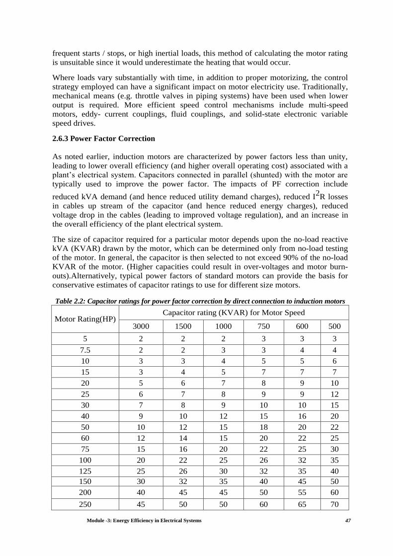
Module -3: Energy Efficiency in Electrical Systems 47
frequent starts / stops, or high inertial loads, this method of calculating the motor rating
is unsuitable since it would underestimate the heating that would occur.
Where loads vary substantially with time, in addition to proper motorizing, the control
strategy employed can have a significant impact on motor electricity use. Traditionally,
mechanical means (e.g. throttle valves in piping systems) have been used when lower
output is required. More efficient speed control mechanisms include multi-speed
motors, eddy- current couplings, fluid couplings, and solid-state electronic variable
speed drives.
2.6.3 Power Factor Correction
As noted earlier, induction motors are characterized by power factors less than unity,
leading to lower overall efficiency (and higher overall operating cost) associated with a
plant’s electrical system. Capacitors connected in parallel (shunted) with the motor are
typically used to improve the power factor. The impacts of PF correction include
reduced kVA demand (and hence reduced utility demand charges), reduced I2R losses
in cables up stream of the capacitor (and hence reduced energy charges), reduced
voltage drop in the cables (leading to improved voltage regulation), and an increase in
the overall efficiency of the plant electrical system.
The size of capacitor required for a particular motor depends upon the no-load reactive
kVA (KVAR) drawn by the motor, which can be determined only from no-load testing
of the motor. In general, the capacitor is then selected to not exceed 90% of the no-load
KVAR of the motor. (Higher capacities could result in over-voltages and motor burn-
outs).Alternatively, typical power factors of standard motors can provide the basis for
conservative estimates of capacitor ratings to use for different size motors.
Table 2.2: Capacitor ratings for power factor correction by direct connection to induction motors
Motor Rating(HP) Capacitor rating (KVAR) for Motor Speed
3000 1500 1000 750 600 500
5 2 2 2 3 3 3
7.5 2 2 3 3 4 4
10 3 3 4 5 5 6
15 3 4 5 7 7 7
20 5 6 7 8 9 10
25 6 7 8 9 9 12
30 7 8 9 10 10 15
40 9 10 12 15 16 20
50 10 12 15 18 20 22
60 12 14 15 20 22 25
75 15 16 20 22 25 30
100 20 22 25 26 32 35
125 25 26 30 32 35 40
150 30 32 35 40 45 50
200 40 45 45 50 55 60
250 45 50 50 60 65 70

Module -3: Energy Efficiency in Electrical Systems 48
Since a reduction in line current, and associated energy efficiency gains, are reflected
backwards from the point of application of the capacitor, the maximum improvement in
overall system efficiency is achieved when the capacitor is connected a cross the motor
terminals, as compared to somewhere further upstream in the plant’s electrical system.
However, economies of scale associated with the cost of capacitors and the labor
required to install them will place an economic limit on the lowest desirable capacitor
size.
Energy managers can, by a motor load survey, arrive at capacitor ratings, locations and
cost benefits. One factor to be considered “operating hours” of motor.
2.6.4 Maintenance
Inadequate maintenance of motors can significantly increase losses and lead to
unreliable operation. For example, improper lubrication can cause increased friction in
both the motor and associated drive transmission equipment. Resistance losses in the
motor, which rise with temperature, would increase. Providing adequate ventilation and
keeping motor cooling ducts clean can help dissipate heat to reduce excessive losses.
The life of the insulation in the motor would also be longer: for every 100
C increase in
motor operating temperature over the recommended peak, the time before rewinding
would be needed is estimated to be halved.
A check list of good maintenance practices to help insure proper motor operation would
include:
Inspecting motors regularly for wear in bearings and housings (to reduce
frictional losses) and for dirt/dust in motor ventilating ducts (to ensure proper
heat dissipation).
Checking load conditions to ensure that the motor is not over or under loaded. A
change in motor load from the last test indicates a change in the driven load, the
cause of which should be understood.
Lubricating appropriately. Manufacturers generally give recommendations for
how and when to lubricate their motors. In adequate lubrication can cause
problems, as noted above. Over-lubrication can also create problems, e.g. excess
oil or grease from the motor bearings can enter the motor and saturate the motor
insulation, causing premature failure or creating a fire risk.
Checking periodically for proper alignment of the motor and the driven
equipment. Improper alignment can cause shafts and bearings to wear quickly,
resulting in damage to both the motor and the driven equipment.
Ensuring that supply wiring and terminal box are properly sized and installed.
Inspect regularly the connections at the motor and starter to be sure that they are
clean and tight.
2.6.5 Age
Most motor cores are manufactured from silicon steel or de-carbonized cold-rolled steel,
the electrical properties of which do not change measurably with age. However, poor
maintenance (inadequate lubrication of bearings, insufficient cleaning of air cooling
passages, etc.) can cause a deterioration in motor efficiency overtime. Ambient

Module -3: Energy Efficiency in Electrical Systems 49
conditions can also have a detrimental effect on motor performance. For example,
excessively high temperatures, high dust loading, corrosive atmosphere, and humidity
can impair insulation properties; mechanical stresses due to load cycling can lead to
mis-alignment. However, with adequate care, motor performance can be maintained.
2.6.6 Rewinding Effects on Energy Efficiency
It is common practice in industry to rewind burnt-out motors. The population of
rewound motors in some industries exceeds 50% of the total population. Careful
rewinding can sometimes maintain motor efficiency at previous levels, but in most
cases, losses in efficiency result. Rewinding can affect a number of factors that
contribute to determining motor efficiency: winding and slot design, winding material,
insulation performance, and operating temperature. For example, a common problem
occurs when heat is applied to strip old windings: the insulation between laminations
can be damaged, thereby increasing eddy current losses. A change in the air gap may
affect power factor and output torque.
However, if proper measures are taken, motor efficiency can be maintained, and in some
cases increased, after rewinding. Efficiency can be improved by changing the winding
design, though the power factor could be affected in the process. Using wires of greater
cross section, slot size permitting, would reduce stat or losses thereby increasing
efficiency. However, it is generally recommended that the original design of the motor
be preserved during the rewind, unless there are specific, load-related reasons for
redesign.
The Impact of rewinding on motor efficiency and power factor can be easily assessed if
the no-load losses of a motor are known before and after rewinding. Maintaining
documentation of no-load losses and no-load speed from the time of purchase of each
motor can facilitate assessing this impact.
Monitoring Format for Rewound Motors
Section Equipment
Code
Motor
Code Motor Type No Load Current
Starter
Resistance/phase No load loss
Sq.Cage Slip
Ring
New
Motor
After
Rewinding New Rewound New Rewound
A V A V Watts Watts
2.6.7 Speed Control of AC Induction Motors
Traditionally, DC motors have been employed when variable speed capability was
desired. By controlling the armature (rotor) voltage and field current of a separately-
excited DC motor, a wide range of output speeds can be obtained. DC motors are
available in a wide range of sizes, but their use is generally restricted to a few low
speed, low-to-medium power applications like machine tools and rolling mills because
of problems with mechanical commutation at large sizes. Also, they are restricted for

Module -3: Energy Efficiency in Electrical Systems 50
use only in clean, non-hazardous areas because of the risk of sparking at the brushes.
DC motors are also expensive relative to AC motors.
Because of the limitations of DC systems, AC motors are increasingly the focus for
variable speed applications. Both AC synchronous and induction motors are suitable for
variable speed control. Induction motors are generally more popular, because of their
ruggedness and lower maintenance requirements. AC induction motors are inexpensive
(half or less of the cost of a DC motor) and also provide a high power to weight ratio
(about twice that of a DC motor).
An induction motor is a synchronous motor, the speed of which can be varied by
changing the supply frequency. The speed can be also be varied through a number of
other means, including varying the input voltage, varying the resistance of the rotor
circuit, using multi- speed windings, using mechanical means such as gears and pulleys
or static voltage and frequency converters. The control strategy to be adopted in any
particular case will depend on a number of factors including investment cost, load
reliability and any special control requirements. Thus, for any particular application, a
detailed review of the load characteristics, historical data on process flows, the features
required of the speed control system, the electricity tariffs and the investment costs
would be a prerequisite to the selection of a speed control system.
The characteristics of the load are particularly important. Load refers essentially to the
torque output and corresponding speed required. Loads can be broadly classified as
constant torque, variable torque and constant power. Constant torque loads are those for
which the output power requirement may vary with the speed of operation but the torque
does not vary. Conveyors, rotary kilns, and constant-displacement pumps are typical
examples of constant torque loads. Variable torque loads are those for which the torque
enquired varies with the speed of operation. Centrifugal pump sand fans are typical
examples of variable torque loads (torque varies as the square of the speed). Constant
power loads are those for which the torque requirements typically change inversely with
speed. Machine tools are atypical example of a constant power load.
The largest potential for electricity savings with variable speed drives is generally in
variable torque applications, for example centrifugal pumps and fans, where the power
requirement changes as the cube of speed. Constant torque loads are also suitable for
VSD application.
Quantifying the magnitude and temporal variation of the load in any specific case is
difficult without adequate instrumentation and an effective monitoring system. For
example, for pumping application, measured data on variations in flow, pressure,
temperature, head, voltage, current and power would be required along with matched
data on production, product mix or grade (if applicable), power supply interruptions,
changes due to seasonal variations (if applicable), planned or unplanned shut downs,
and effect of start- upon process energy requirements. Extensive data of this form
typically are not available. However, in many applications, equipment is over sized due
to the safety margins applied at each stage of the system design, in which cases a
simpler analysis based on fewer or not significant savings are possible.

Module -3: Energy Efficiency in Electrical Systems 51
Electro-Mechanical Speed Control Systems
Electro-mechanical speed control mechanisms include purely mechanical systems,
multi- speed motors, eddy-current drives, and fluid couplings. The characteristics of
these are summarized in the table below.
i. Gears, pulleys, etc.
A variety of purely mechanical systems are available for motor speed control, including
variable pulley sheaves, gears, chains, and friction drives. These systems provide
limited speed variation and do not lend themselves to automatic control, but are suitable
for applications which require operation at a few fixed speeds and adjustment at in
frequent intervals.
ii. Multi-speed motors
Motors can be wound such that two speeds, in the ratio of 2:1, can be obtained. Motors
can also be wound with two separate windings, each giving 2 operating speeds, for a
total off our speeds. Multi-speed motors can be designed for applications involving
constant torque, variable torque, or for constant output power. Multi-speed motors are
suitable for applications which require limited speed control (two or three fixed speeds
instead of continuously variable speed), in which cases they tend to be very economical.
Table 2.3: Electro Mechanical Speed Control alternatives for AC Induction Motors
VSD Type (Power,
Speed Range) Advantages Disadvantages
ELECTRO-MECHANICAL CONTROL METHODS
Gears, Pulleys, etc.
Variable Pulley
Sheaves Low Cost
Low power savings; high
maintenance costs
Gears Low Cost Low power savings; high
maintenance costs
Chains Low Cost Low power savings; high
maintenance costs
Friction Drives Low Cost Low power savings; high
maintenance costs
Multispeed Motors Operational at 2 or
4FixedSpeeds
Stepped speed control;
lower efficiency than single-speed
motors
Eddy-current Drives
>0kW, 10:1
Simple; relatively low
cost; step less speed
control
Needs low efficiency at below 50%
rated speed
Fluid Coupling
Drives>0 kW, 5: 1
Simple; relatively low
cost; stepless speed
control
Low efficiency at below 50% rated
speed

Module -3: Energy Efficiency in Electrical Systems 52
iii. Eddy-current drives
This method employs a needy-current clutch to vary the output speed. The clutch
consists of a primary member coupled to the shaft of the motor and a freely revolving
secondary member coupled to the load shaft. The secondary member is separately
excited using a DC field winding. The motor starts with the load at rest and a DC
excitation is provided to the secondary member which induces eddy-currents in the
primary member. The interaction of the fluxes produced by the two currents gives rise
to a torque at the load shaft. By varying the DC excitation the output speed can be
varied to match the load requirements. The major disadvantage of this system is
relatively poor efficiency, particularly at low speeds.
iv. Fluid-coupling drives
Power can be transmitted through a fluid either by hydro-static, hydro-kinetic, hydro-
viscous, or hydro-dynamic forces. In most commercial fluid coupling drives, normally a
light mineral oil, which in turn transmits the energy to the load.
Figure 2.7: Fluid Coupling
Construction
Fluid couplings work on the hydrodynamic principle. It consists of a pump-generally
known as impeller and a turbine generally known as rotor, both enclosed suitably in a
casing. The impeller and the rotor are bowl-shaped and have large number of radial
vanes. They face each other with an air gap. The impeller is suitably connected to the
prime mover while the rotor has a shaft bolted to it. This shaft is further connected to the
driven machine through a suitable arrangement. Oil is filled in the fluid coupling from
the filling plug provided on its body. A fusible plug is provided on the fluid coupling
which blows off and drains out oil from the coupling in case of sustained overloading.

Module -3: Energy Efficiency in Electrical Systems 53
Operating Principle
There is no mechanical inter-connection between the impeller and the rotor and the
power is transmitted by virtue of the fluid filled in the coupling. When the impeller is
rotated by the prime mover, the fluid flows out radially and then axially under the action
of centrifugal force. It then crosses the air gap to the runner and is directed towards the
bowl axis and back to the impeller. To enable the fluid to flow from impeller to rotor it
is essential that there is difference in head between the two and thus it is essential that
there is difference in RPM known as slip between the two. Slip is an important and
inherent characteristic of a fluid coupling resulting in several desired advantages. As the
slip increases, more and more fluid can be transferred. However when the rotor is at a
standstill, maximum fluid is transmitted from impeller to rotor and maximum torque is
transmitted from the coupling. This maximum torque is the limiting torque. The fluid
coupling also acts as a torque limiter.
Characteristics
Fluid coupling has a centrifugal characteristic during starting thus enabling no-load
start-up of prime mover, which is of great importance. This feature also provides
inherent overload protection. The slipping characteristic of fluid coupling provides a
wide range of choice of power transmission characteristics. By varying the quantity of
oil filled in the fluid coupling, the normal torque transmitting capacity can be varied.
The maximum torque or limiting torque of the fluid coupling can also be set to a pre-
determined safe value by adjusting the oil filling. The fluid coupling has the same
characteristics in both directions of rotation.
The losses in this system are circulation and slip losses. Circulation losses are a constant
percentage of the rated capacity of the unit—typically 1.5%. Slip losses are the product
of torque output and slip speed (motor speed minus load speed). If the slip speed
increases significantly, a higher motor rating, or a motor designed for high slip may
have to be selected.
v. Variable Pitch Drives Description
This method of speed control uses the mechanical means of belts and variable pitch
sheaves or pulleys to change speed. The power source is a standard induction motor.
Often these units are enclosed and have a gear reducer built in for reduced speed ranges.
The horse power range is generally limited from 5 to 50HP with not much available
outside of that range.
Variable Pitch Features
First cost – These systems are among the lowest cost methods of achieving variable
speed.
Simplicity – The principle of operation is well known and easy to understand. Also the
construction is simple.

Module -3: Energy Efficiency in Electrical Systems 54
Variable Pitch Disadvantages
Control – Remote control is not an inherent feature. Since the drive uses mechanical
means to vary the speed, electrical control signals must be adapted to existing
mechanical controls.
Belt wear–The stress of variable speed operation requires periodic checks and
replacement of the belts.
High inertia loads – This condition may cause problems. It may require over sizing the
drive or custom motors. Special shutdown and start up procedures may be required to
prevent overloading the motor.
Sheave Wear – running at a constant speed for extended periods of time may cause
grooving in the sheaves. This degrades speed control and decreases belt life.
Motor Speed Control Systems
Multi-speed motors
Motors can be wound such that two speeds, in the ratio of 2:1, can be obtained. Motors
can also be wound with two separate windings, each giving 2 operating speeds, for a
total of four speeds. Multi-speed motors can be designed for applications involving
constant torque, variable torque, or for constant output power. Multi-speed motors are
suitable for applications, which require limited speed control (two or four fixed speeds
instead of continuously variable speed), in which cases they tend to be very economical.
They have lower efficiency than single-speed motors
Direct Current Drives (DC)
The DC drive technology is the oldest form of electrical speed control. The drive
system consists of a DC motor and a controller. The motor is constructed with armature
and field windings. Both of these windings require a DC excitation for motor operation.
Usually the field winding is excited with a constant level voltage from the controller.
Then, applying a DC voltage from the controller to the armature of the motor will
operate the motor. The armature connections are made through a brush and commutator
assembly. The speed of the motor is directly proportional to the applied voltage.
The controller is a phase controlled bridge rectifier with logic circuits to control the DC
voltage delivered to the motor armature. Speed control is achieved by regulating the
armature voltage to the motor. Often a tachogenerator is included to achieve good
speed regulation. The tachogenerator would be mounted on the motor and produces a
speed feedback signal that is used within the controller.
Wound Rotor AC Motor Drives (Slip Ring Induction Motors)
Wound rotor motor drives use a specially constructed motor to accomplish speed
control. The motor rotor is constructed with windings which are brought out of the
motor through slip rings on the motor shaft. These windings are connected to a
controller which places variable resistors in series with the windings. The torque

Module -3: Energy Efficiency in Electrical Systems 55
performance of the motor can be controlled using these variable resistors. Wound rotor
motors are most common in the range of 300 HP and above.
Slip Power Recovery Systems
Slip power recovery is a more efficient alternative speed control mechanism for use
with slip-ring motors. In essence, a slip power recovery system varies the rotor voltage
to control speed, but instead of dissipating power through resistors, the excess power is
collected from the slip rings and returned as mechanical power to the shaft or as
electrical power back to the supply line. Because of the relatively sophisticated
equipment needed, slip power recovery tends to be economical only in relatively high
power applications and where the motor speed range is 1:5 or less.
Application of Variable Speed Drives (VSD)
Although there are many methods of varying the speeds of the driven equipment such as
hydraulic coupling, gear box, variable pulley etc., the most possible method is one of
varying the motor speed itself by varying the frequency and voltage by a variable
frequency drive.
Concept of Variable Frequency Drive
The speed of an induction motor is proportional to the frequency of the AC voltage
applied to it, as well as the number of poles in the motor stator. This is expressed by the
equation:
RPM = (f x 120) / p
Where f is the frequency in Hz, and p is the number of poles in any multiple of 2.
Therefore, if the frequency applied to the motor is changed, the motor speed changes in
direct proportion to the frequency change. The control of frequency applied to the motor
is the job given to the VSD.
The VSD's basic principle of operation is to convert the electrical system frequency and
voltage to the frequency and voltage required to drive a motor at a speed other than its
rated speed. The two most basic functions of a VSD are to provide power conversion
from one frequency to another, and to enable control of the output frequency.
Need for VFD
Earlier motors tended to be over designed to drive a specific load over its entire range.
This resulted in a highly inefficient driving system, as a significant part of the input
power was not doing any useful work. Most of the time, the generated motor torque was
more than the required load torque.
In many applications, the input power is a function of the speed like fan, blower, pump
and so on. In these types of loads, the torque is proportional to the square of the speed
and the power is proportional to the cube of speed. Variable speed, depending upon the
load requirement, provides significant energy saving. A reduction of 20% in the
operating speed of the motor from its rated speed will result in an almost 50% reduction

Module -3: Energy Efficiency in Electrical Systems 56
in the input power to the motor. This is not possible in a system where the motor is
directly connected to the supply line. In many flow control applications, a mechanical
throttling device is used to limit the flow. Although this is an effective means of control,
it wastes energy because of the high losses and reduces the life of the motor valve due to
generated heat
.
Figure: 2.8 Components of a Variable Speed Drive
Principles of VFD’s
The VFD is a system made up of active/passive power electronics devices (IGBT,
MOSFET, etc.), a high speed central controlling unit and optional sensing devices,
depending upon the application requirement. A typical modern-age intelligent VFD for
the three phase induction motor is shown in Figure 2.10.
The basic function of the VFD is to act as a variable frequency generator in order to
vary speed of the motor as per the user setting. The rectifier and the filter convert the
AC input to DC with negligible ripple. The inverter, under the control of the
microcontroller, synthesizes the DC into three-phase variable voltage, variable
frequency AC.
The base speed of the motor is proportional to supply frequency and is inversely
proportional to the number of stator poles. The number of poles cannot be changed once
the motor is constructed. So, by changing the supply frequency, the motor speed can be
changed. But when the supply frequency is reduced, the equivalent impedance of
electric circuit reduces. This results in higher current drawn by the motor and a higher
flux. If the supply voltage is not reduced, the magnetic field may reach the saturation
level. Therefore, in order to keep the magnetic flux within working range, both the
supply voltage and the frequency are changed in a constant ratio. Since the torque
produced by the motor is proportional to the magnetic field in the air gap, the torque
remains more or less constant throughout the operating range.

Module -3: Energy Efficiency in Electrical Systems 57
Figure 2.9: V/f Control
As seen in Figure 2.11, the voltage and the frequency are varied at a constant ratio up to
the base speed. The flux and the torque remain almost constant up to the base speed.
Beyond the base speed, the supply voltage cannot be increased. Increasing the frequency
beyond the base speed results in the field weakening and the torque reduces. Above the
base speed, the torque governing factors become more nonlinear as the friction and wind
age losses increase significantly. Due to this, the torque curve becomes nonlinear. Based
on the motor type, the field weakening can go up to twice the base speed. This control is
the most popular in industries and is popularly known as the constant V/f control.
By selecting the proper V/f ratio for a motor, the starting current can be kept well under
control. This avoids any sag in the supply line, as well as heating of the motor. The VFD
also provides over current protection. This feature is very useful while controlling the
motor with higher inertia. Since almost constant rated torque is available over the entire
operating range, the speed range of the motor becomes wider. User can set the speed as
per the load requirement, thereby achieving higher energy efficiency (especially with
the load where power is proportional to the cube speed). Continuous operation over
almost the entire range is smooth, except at very low speed. This restriction comes
mainly due to the inherent losses in the motor, like frictional, wind age, iron, etc. These
losses are almost constant over the entire speed. Therefore, to start the motor, sufficient
power must be supplied to overcome these losses and the minimum torque has to be
developed to overcome the load inertia.
A single VFD has the capability to control multiple motors. The VFD is adaptable to
almost any operating condition.
VFD Selection
The size of the VFD depends mainly on driven load type and characteristics. This will
determine the drive capacity in terms of full load current (FLC) and power delivered
(kW).
Driven Load Types and Characteristics
Mechanical load, which is the load on the motor shaft, can be of two types- Constant
Torque (CT) or Variable Torque (VT). There is a basic difference between the two loads
with respect to load torque variation at different speeds.
A CT load implies that the load torque seen at motor shaft is independent of motor
speed.

Module -3: Energy Efficiency in Electrical Systems 58
This means that the load torque remains approximately the same at all speeds. Examples
of CT loads include material handling conveyers, reciprocating & screw compressors
and certain types of blowers such as roots blower.
A VT load implies that the load torque seen at the motor shaft is dependent upon the
motor speed.
Examples of VT loads include centrifugal fans & pumps and centrifugal compressors.
The graphs (Figures 2.10 & 2.11) below describe the torque requirements at various
speeds.
Figure 2.10 A CT load characteristic Figure 2.11 A VT load characteristic
Variable Frequency Drives: Precautions
• Ensure that the power voltage supplied to VFDs is stable with inplusorminus10% to
prevent tripping faults.
• Motors operating at low speeds can suffer from reduced cooling. For maximum
protection on motors to be run at low speeds, install thermal sensors that inter lock with
the VFD control circuit. Standard motor protection responds only to over-current.
• Speed control wiring, which is often 4 mA to 20 m A or 0 VDC to 5 VDC, should be
separated from other wiring to avoid erratic behavior. Parallel runs of 115V and 24 V
control wiring may cause problems.
• Precautions for specifying, installing and operating VFDs are numerous. Improper
installation and start-up accounts for 50 % of VFD failures
• Use the VFD start-up sheet to guide the initialization check prior to energizing the VFD
for the first time.
• Corrosive environments, humidity above 95%, ambient air temperatures exceeding 400C
(1040F), and conditions where condensation occurs may damage VFDs.
• If a VFD is started when the load is already spinning, the VFD will try to pull the motor
down to a low, soft-start frequency. This can result in high current and a trip unless
special VFDs are used.
• Switching from grid power to emergency power while the VFD is running is not
possible with most types of VFDS. If power switching is anticipated, include this
capacity in the specification.
• If electrical disconnects are located between the VFD and motor, interlock the run-
permissive circuit to the disconnect.
Load Torque Motor Shaft Power
Motor Shaft Speed (RPM) Motor Shaft Speed (RPM)

Module -3: Energy Efficiency in Electrical Systems 59
• If a motor always operates at rated load, a VFD will increase power use, due to
electrical losses in the VFD.
Harmonics
A key concern with VSD operation is the generation of harmonics-multiples of the
fundamental frequency (50Hz) which result in an on-sinusoidal high for in verters with
only a few pulses per second as compared to more complex ones that produce a12-step
(or higher) voltage waveform or that employ pulse width modulation.
Harmonics increase motor losses, and can adversely affect the operation of sensitive
auxiliary equipment. Then on-sinusoidal supply results in harmonic currents in the stator
which increases the total current draw. In addition, the rotor resistance (or more
precisely impedance) increases significantly at harmonic frequencies, leading to less
efficient operation. Also, stray load losses can increase significantly at harmonic
frequencies. Overall motor losses increase by about 20% with a six-step voltage wave
form compared to operation with a sinusoidal supply. In some cases the motor may have
to be de rated as a result of the losses. Alternatively, additional circuitry and switching
devices can be employed to minimize losses.
Motor instability, characterized by hunting of the rotor (a phenomenon where the rotor
accelerates or decelerates about a stable speed), may occur for certain critical frequency
ranges and loading conditions. Motors are inherently unstable at low frequencies.
Instability can also occur due to the interaction between the motor and the converter.
This is especially true of motors of low rating, which have low inertia. Instabilities can
be reduced by changing the machine parameters (e.g., motor impedance) or by
employing closed loop feedback systems. The VSD supplier should be consulted to
ascertain the impact of inverters on motor performance.
Harmonics can also contribute to low power factor. Shunt capacitors that might be used
to compensate for low power factor also generate harmonics. If parallel resonance
occurs between the shunt capacitor and VSD (at frequency determined by the
capacitance and system inductance), the voltage wave form may undergo significant
distortion causing motor overheating, capacitor failure or mis-operation of the control.
To avoid resonance, reactive filters can be designed for the VSD. Filters are designed to
eliminate resonance at the fifth and seventh frequency harmonics which are the most
harmful7. Low level distortions may still be present, but these do not pose a serious
problem.
2.6.8 Other operating concerns
Steep voltage transients, e.g. caused by switching of shunt capacitors or transient system
faults, can affect VSD operation. Isolation transformers or special VSD inverter designs
can be used to prevent such transients from tripping or otherwise affecting VSD
operation. A power supply with unstable voltage and frequency also hampers
regenerative braking, thus eroding efficiency.
When a totally-enclosed fan-cooled motor is controlled to operate at very low speed,
some de rating may be required if the cooling is inadequate.

Module -3: Energy Efficiency in Electrical Systems 60
In cases where some of the operating time is at close to rated load, system efficiency
might be increased by using a bypass arrangement to avoid the losses in the VSD. The
VSD would be engaged at lower loads, when the VSD-related reductions in power
would more than off-set in efficiencies of the VSD. Such a bypass arrangement would
also provide for greater reliability in case of a VSD failure.
2.6.9 Transmission Efficiency
Power transmission equipment linking motors to driven machines including shafts,
belts, chains, and gears should be properly selected, installed and maintained. When
possible, use flat belts in place of V-belts. Helical gears are more efficient than worm
gears; use worm gears only with motors under 10hp. As far as possible it is better to
have a direct drive thus avoiding losses in motor power transmission to the driven
machine.
Power transmission Efficiency margin from V belt drive flat belt drive 5 to 6 % and from
Worm gearbox to Helical Gearbox 8 to 10 %
2.6.10 Soft Starters
A soft starter is another form of reduced voltage starter for A.C. induction motors which
facilities gradual acceleration of motor and consequent elimination of shocks during
starting (soft start). The starting current with a soft starter is only1.5 to 2 times the full
load current as against 5–7 times in the case of other conventional starters. Because of
this cable sizes, contact or sand motors can be sized lower during the initial selection.
The soft starter is similar to a primary resistance or primary reactance starter i n that it is
in series with the supply to the motor. The
currentintothestarterequalsthecurrentout.Thesoftstarteremployssolid state devices to
control the current flow and therefore the voltage applied to the motor.
Working of Soft Starter / Energy Saver
i. The soft-start motor starter combines the advantages of reduced voltage starting
and reduced energy consumption, in one compact economic package. Because
they are solid state, burnout of starter parts are eliminated. The reduced voltage
starter gracefully increases motor voltage from the set minimum voltage to full
voltage allowing the motor to smoothly and gradually accelerate to full speed,
when it is set on soft-start mode.
ii. The soft starter offers a ramp input voltages source to a motor which can be
programmable, and this factor is the essence of soft starting as against
conventional step voltage starter or D.O.L. starter.
Advantages:
• Nanosecond response on account of micro-electronics involved.
• Reducedpowerconsumptionandhencereducedenergybills,atpartloads.Power
factor improvement on a continuous basis
• Reduction in maximum demand

Module -3: Energy Efficiency in Electrical Systems 61
• Reduced peak motor current during starting
• Reducedmotortemperature,increasedmotorlifeanddecreasedmaintenanceneeds
• When using a generator, the power generated can be used to operate more
equipment, since the starting and running currents of motors are lower, when
motors are fitted with energy-saver-soft-starters.
Typical Applications
Plastic injection moulding machines, Machine tools / motor generator welding sets,
chemical process equipment, unloading type air compressors, punch presses, center less
grinding and polishing machines, blowers, wherever the motor load is varying
continuously.
2.7 Case Studies
CASE STUDY- 1
Based on study of humidification plants in a Rayon industry, it was established that the
air flow demand in supply air and return air varies as per season and the supply and
return fans rated 16 kW, 12 kW respectively were running at constant load. Towards
energy efficiency improvement, the drives were converted variable frequency drives.
The part load effects one summarized as follows:
Supply Frequency
C/S
Supply Air Fan Return Air Fan
KW Drawn % Drop in KW Drawn % Drop in
50 16.4 Capacity Ref. 12 Capacity Ref.
45 12.0 10.0 8.7 10.0
40 8.4 20.0 6.1 20.0
35 5.6 30.0 4.1 30.0
30 3.5 40.0 2.6 40.0
As the flow requirements vary, the following schedule was adopted with power savings
indicated alongside.
Months Recommended
Frequency
Average %kW Savings
October, Nov, Dec, Jan 35 51
Feb, March, Sept. 40 35
April, August, July 45 18
May, June 50 -
Covering all 10fans, with 142kW consumption among five sets of supply air & return
air fans, the savings achieved were3 77223kWh worth BDT.13.16lakhs/yea against an

Module -3: Energy Efficiency in Electrical Systems 62
investment of BDT12.5lakhs @BDT1.25lakh/ drive yielding a simple payback period of
less than one year.
CASE STUDY-2
Refrigeration plant study in a chemical complex indicated part load operation of
reciprocating compressor drives with unloader mechanism, as illustrated below:
Item Reference Brine Unit Chilled Water Unit
Motor input kW 53 74.1
Rpm 750 780
Op. hours / day 14.5 9.0
% ON time 58 38
Power consumption/day (kWh) 768.5 666.9
The Compressor speed can be increased or decreased with a change in the drive pulley
or the driven pulley or in some cases, both pulleys. By pulley diameter modification, the
machines were de-rated to match required capacity. A higher sized reciprocating
compressor operating with higher unloading percentage was downsized by reducing the
motor (drive) pulley size from 12” to 7.5” in case of Brine unit and 12” to 6” in case of
Chilled water unit .
Despite increased use hours due to de rating effects, the specific power consumption
reduced as the evaporator and condenser became oversized for the de-rated condition,
and the energy consumption reduced as well as follows:
Item Reference Brine Unit Chilled Water Unit
Motor input kW 32.3 35.6
Speed Rpm 480 409.5
Op. hours / day 18.0 14.0
Average energy consumption/day (kWh) 581.4 498.4
The energy savings of 355.6kWh/day by the simple modifications, are a significant
25%. The interesting part of the exercise was that the investment is nominated, and the
pay back is in order of days. Most cases, where load-unload cycling of reciprocating
machine stakes place for capacity control, pulley diameter modification offers a simple,
cheap solution to de rate the machine capacity with energy savings potential of
significant order.

Module -3: Energy Efficiency in Electrical Systems 63
Chapter 3: COMPRESSED AIRSYSTEMS
3.1 Introduction
Air compressors account for a significant amount electricity used in industrial sector.
Air compressors are used in a variety of industries to supply process requirements,
operate pneumatic tools and equipment, and for instrumentation. The generation
efficiency is only about 10% as shown in the figure 3.1 and balance 90% of energy of
the power of the prime mover being converted to unusable heat energy and to a lesser
extent lost in form of friction, misuse and noise. Further considering the distribution
efficiency, the overall efficiency can be as low as 6.5% when pressure drops, leaks,
and part-load control losses are considered.
Figure 3.1: Efficiency of Compressed Air System
3.2 Compressor Types
Compressors are broadly classified as dynamic and positive displacement types.
Dynamic compressors are centrifugal compressors and are further classified as radial
and axial flow types. Positive displacement compressors are further classified as
reciprocating and rotary compressors, under which there are further sub-classifications.
Dynamic compressors increase the fluid’s velocity, which is then converted to increased
pressure at the outlet. Positive displacement compressors increase the pressure of the
gas by reducing the volume. The flow and pressure requirements of a given application
determine the suitability of a particulars type of compressor.
3.3 Positive Displacement Compressors
3.3.1 Reciprocating Compressors
In industry, reciprocating compressors are the most widely used type for both air and
refrigerant compression. They are characterized by a flow output that remains nearly
constant over arrange of discharge pressures. Also, the capacity is directly proportional
to the speed. The output, however, is a pulsating one. Reciprocating compressors are
available in many configurations, the four most widely used of which are horizontal,
vertical, horizontal balance-opposed and tandem. Vertical type reciprocating

Module -3: Energy Efficiency in Electrical Systems 64
compressors are used in the capacity range of 50–150cfm. Horizontal balance opposed
compressors are used in the capacity range of 200–5000 cfm in multi-stage design and
upto 10,000 cfm in single stage designs. In refrigeration cycles, reciprocating
compressors are best suited for applications requiring up to 150 tone of refrigeration.
Reciprocating compressors are available in variety of types, such as single or multiple
cylinder, single or multi stage, lubricated and non -lubricated, and water or air cooled.
Non- lubricated compressors are especially useful for providing instrument air and for
processes, which require oil free discharge. However non- lubricated machines have
marginally higher specific power consumption (kW/cfm) as compared to lubricated
models. In the case of lubricated machines, oil has to be separated from the discharge.
Single cylinder machines are generally air-cooled while multi-cylinder machines are
water cooled, though multi-stage air cooled models are available for machines up to 100
kW. Two stage machines are used for high pressures and are characterized by lower
discharge temperature (140 – 1600C) compared to single-stage machines (205 – 2400C).
In some cases, multi-stage machines may have a lower specific power consumption
compared to single stage machines operating over the same total pressure differential.
Multi- stage machines generally have higher investment costs, particularly for
applications with high discharge pressure (up to 7 bar) and low capacities (less than 25
cfm). Multi staging has other benefits, however, including a reduced pressure
differential across cylinders, which reduces the load and stress on valves and piston
rings.
3.3.2 Rotary Compressors
Rotary compressors have rotors in place of pistons and give a continuous, pulsation free
discharge. They operate at high speed and generally provide higher throughput than
reciprocating compressors. They are directly coupled to the prime mover and require
lower starting torque as compared to reciprocating machines. Also they do not require
specialized foundations, operate with limited vibration, and have a lower number of
parts - which means less failure rate. Among rotary machines, the lobe compressor (also
known as a Roots blower) and screw compressors are among the most widely used. The
lobe compressor is essentially a low pressure blower and is limited to a discharge
pressure of 1barin single-stage design and up to 2.2 bar in two stage design. Screw
compressors are high speed, high capacity machines and are available in both dry and
oil injected types with single or twin screw compressors deliver oil-free air and are
available in sizes up to 20,000cfm and pressure up to 15 bar, and in the size range of
100 – 1000cfm in lubricated designs upto 10 bar discharge pressure. They cannot
operate at discharge pressures below 3.5 bar. In the case of oil injected (lubricated)
rotary screw compressors, oil has to be separated from the discharged air (gas). In
refrigeration systems, screw compressors are preferable for intermediate temperatures
(10 to 50oC).
Other types of rotary compressors such as rotary vane and liquid-ring compressors are
also available. Rotary vane compressors are small in size and have a pulsation-free
output. The two common types of rotary vane compressors are oil-flooded with non-
metallic blades and water-cooled with steel blades. Both designs have many of the
advantages of the oil injected screw compressor and are generally designed as multi-
stage machines. Single-stage designs are available for discharge pressures up to 7 bar.
Liquid ring compressors operate on the same principle as rotary vane compressors. They
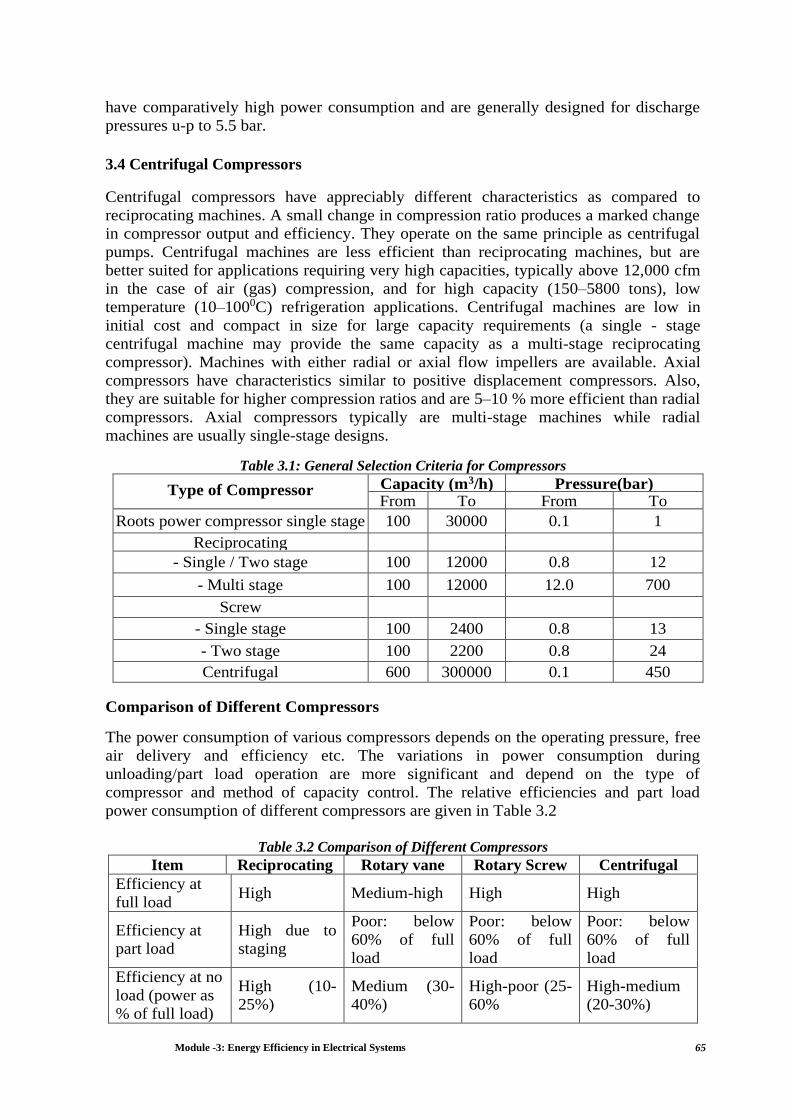
Module -3: Energy Efficiency in Electrical Systems 65
have comparatively high power consumption and are generally designed for discharge
pressures u-p to 5.5 bar.
3.4 Centrifugal Compressors
Centrifugal compressors have appreciably different characteristics as compared to
reciprocating machines. A small change in compression ratio produces a marked change
in compressor output and efficiency. They operate on the same principle as centrifugal
pumps. Centrifugal machines are less efficient than reciprocating machines, but are
better suited for applications requiring very high capacities, typically above 12,000 cfm
in the case of air (gas) compression, and for high capacity (150–5800 tons), low
temperature (10–1000C) refrigeration applications. Centrifugal machines are low in
initial cost and compact in size for large capacity requirements (a single - stage
centrifugal machine may provide the same capacity as a multi-stage reciprocating
compressor). Machines with either radial or axial flow impellers are available. Axial
compressors have characteristics similar to positive displacement compressors. Also,
they are suitable for higher compression ratios and are 5–10 % more efficient than radial
compressors. Axial compressors typically are multi-stage machines while radial
machines are usually single-stage designs.
Table 3.1: General Selection Criteria for Compressors
Type of Compressor Capacity (m3/h) Pressure(bar) From To From To
Roots power compressor single stage 100 30000 0.1 1
Reciprocating
- Single / Two stage 100 12000 0.8 12
- Multi stage 100 12000 12.0 700
Screw
- Single stage 100 2400 0.8 13
- Two stage 100 2200 0.8 24
Centrifugal 600 300000 0.1 450
Comparison of Different Compressors
The power consumption of various compressors depends on the operating pressure, free
air delivery and efficiency etc. The variations in power consumption during
unloading/part load operation are more significant and depend on the type of
compressor and method of capacity control. The relative efficiencies and part load
power consumption of different compressors are given in Table 3.2
Table 3.2 Comparison of Different Compressors
Item Reciprocating Rotary vane Rotary Screw Centrifugal
Efficiency at
full load High Medium-high High High
Efficiency at
part load
High due to
staging
Poor: below
60% of full
load
Poor: below
60% of full
load
Poor: below
60% of full
load
Efficiency at no
load (power as
% of full load)
High (10-
25%)
Medium (30-
40%)
High-poor (25-
60%
High-medium
(20-30%)

Module -3: Energy Efficiency in Electrical Systems 66
In case of reciprocating machines, the unload power consumption is in the order of 25%
of full load power. While in screw compressors, the unload power consumption is
marginally higher compared to reciprocating machines.
It is preferable to use screw compressors for constant air requirement. If screw
compressors have to be installed for fluctuating loads, it is desirable to have screw
compressor with variable speed drive to further optimize unload power consumption.
Some of the plants have adopted the strategy of operating screw compressor at full load
for meeting the base-load requirement and reciprocating compressor for fluctuating load
to optimize on unload power consumption.
3.5 System Components
Compressed air systems, depending on the requirement, consist of a number of
components compressors filters, air dryers, inter-coolers, after coolers, oil separators,
valves, nozzles, and piping.
• Intake Air Filters: Prevent dust and atmospheric impurities from entering
compressor. Dust causes sticking valves, scored cylinders, excessive wear etc.
• Inter-stage Coolers: Reduce the temperature of the air(gas) before it enters
the next stage to reduce the work of compression and increase efficiency.
They can be water-or air-cooled.
• After Coolers: Reduce the temperature of the discharge air, and thereby
reduce the moisture carrying capacity of air.
• Air-dryers: Air dryers are used to remove moisture, as air for instrument and
pneumatic equipment needs to be relatively free of any moisture. The moisture
is removed by suing ads or bents or refrigerant dryers, or state of the art heat
less dryers.
• Moisture Traps: Air traps are used for removal of moisture in the
compressed air distribution lines. They resembles team traps where in the air
is trapped and moisture is removed.
• Receivers: Depending on the system requirements, one or more air receivers
are generally provided to reduce output pulsations and pressure variations.
3.6 Compressor Performance
Capacity of a Compressor: Free Air Delivery (FAD)
Free air, as defined by CAGI (Compressed Air & Gas Institute) is air at
ATMOSPHERIC conditions at any specific location. Because the barometer and
temperature may vary at different localities and at different times, it follows that this
term does not mean air under standard conditions.
Measured in CFM (Cubic feet per minute) this is the amount of compressed air
converted back to the actual inlet (free air) conditions before it was compressed. In other
words, the volume of air, which is drawn in from the atmosphere by the compressor,
then compressed and delivered at a specific pressure.

Module -3: Energy Efficiency in Electrical Systems 67
Compressor Efficiency Definitions
Compressor efficiency is often expressed as either an adiabatic or isothermal or
mechanical efficiency. These are computed as the isothermal and adiabatic power
respectively, divided by the actual power consumption. The calculation of isothermal
power excludes that needed to overcome friction and generally gives an efficiency that
is lower than a diabetic efficiency. This is an important consideration when selecting
compressors based on reported values of efficiency. Manufacturers generally provide
the adiabatic (theoretical) horse power required for compression. The actual power in
take would be slightly higher because of mechanical losses.
For practical purposes, the most effective guide in comparing compressor efficiencies is
the specific power consumption for different compressors that would provide identical
duty.
Isothermal Efficiency
The Iso-thermal efficiency of a multi-stage air compressor can be calculated as a ratio of
the theoretical kW required for a duty conditions and the actual kW input measured.
This efficiency would reflect the combined efficiency of the compressor and the drive
motor and the method can be adopted to assess the performance for identifying margins
with respect to rated values, merit rating of compressors, maintenance planning, etc.
N = No. of stages
K = Ratio of specific heats (1.35 for air)
Ps = suction pressure in kg/cm2
Pd = Discharge pressure in kg/cm2
Q = Actual air flow (m3
/min.) Actual kW = √ 3 V I × PF as measured
Efficiency of compressor and motor combination =
It is also a done thing, to compute and add-up stage wise work of compression
(theoretical kW) in case the performance of intercoolers is not optimal.
Volumetric Efficiency
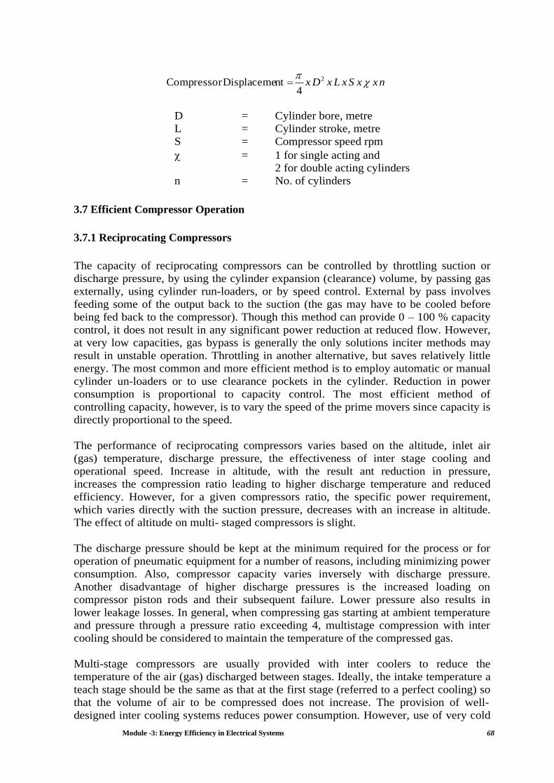
Module -3: Energy Efficiency in Electrical Systems 68
nxxSxLxDx 2
4ntDisplaceme Compressor
D = Cylinder bore, metre
L = Cylinder stroke, metre
S = Compressor speed rpm
= 1 for single acting and
2 for double acting cylinders
n = No. of cylinders
3.7 Efficient Compressor Operation
3.7.1 Reciprocating Compressors
The capacity of reciprocating compressors can be controlled by throttling suction or
discharge pressure, by using the cylinder expansion (clearance) volume, by passing gas
externally, using cylinder run-loaders, or by speed control. External by pass involves
feeding some of the output back to the suction (the gas may have to be cooled before
being fed back to the compressor). Though this method can provide 0 – 100 % capacity
control, it does not result in any significant power reduction at reduced flow. However,
at very low capacities, gas bypass is generally the only solutions inciter methods may
result in unstable operation. Throttling in another alternative, but saves relatively little
energy. The most common and more efficient method is to employ automatic or manual
cylinder un-loaders or to use clearance pockets in the cylinder. Reduction in power
consumption is proportional to capacity control. The most efficient method of
controlling capacity, however, is to vary the speed of the prime movers since capacity is
directly proportional to the speed.
The performance of reciprocating compressors varies based on the altitude, inlet air
(gas) temperature, discharge pressure, the effectiveness of inter stage cooling and
operational speed. Increase in altitude, with the result ant reduction in pressure,
increases the compression ratio leading to higher discharge temperature and reduced
efficiency. However, for a given compressors ratio, the specific power requirement,
which varies directly with the suction pressure, decreases with an increase in altitude.
The effect of altitude on multi- staged compressors is slight.
The discharge pressure should be kept at the minimum required for the process or for
operation of pneumatic equipment for a number of reasons, including minimizing power
consumption. Also, compressor capacity varies inversely with discharge pressure.
Another disadvantage of higher discharge pressures is the increased loading on
compressor piston rods and their subsequent failure. Lower pressure also results in
lower leakage losses. In general, when compressing gas starting at ambient temperature
and pressure through a pressure ratio exceeding 4, multistage compression with inter
cooling should be considered to maintain the temperature of the compressed gas.
Multi-stage compressors are usually provided with inter coolers to reduce the
temperature of the air (gas) discharged between stages. Ideally, the intake temperature a
teach stage should be the same as that at the first stage (referred to a perfect cooling) so
that the volume of air to be compressed does not increase. The provision of well-
designed inter cooling systems reduces power consumption. However, use of very cold
Module -3: Energy Efficiency in Electrical Systems 69
water can result in condensation which may result in water can result in condensation
which may result in water entering the cylinder, thereby reducing valve life, accelerating
wear and scoring of piston, piston rings and cylinder. Condensation can also occur when
the relative humidity of inlet air is high and the compressor cylinder temperature is
lower than inlet air temperature (for example, as a result of higher than required flow of
cooling water). The condensed water may also wash away the oil film on the cylinder
and cause rust which will result in a abrasion during compressor operation and
significantly reduce efficiency. At the other extreme, if cooling is in sufficient, the
discharge temperature increases. High temperature operation reduces oil viscosity and
the oil film thickness can be reduced.
The location of the compressor should be considered during the selection process.
Locations with high moisture or high temperature can cause operational trouble and
increase power consumption. Cooling should be adequate in such cases. When locating
the suction inside buildings, care should be taken to ensure adequate clearance between
the suction and the walls to reduce pulsation and vibrations.
3.7.2 Centrifugal Compressors
Manufacturers specify discharge pressure and power requirement as a function of the
inlet volumetric flow rate. These performance curves are valid at only the given inlet
conditions. Therefore, to optimize process efficiency and to predict performance at
different process and inlet conditions, performance curves which provide the polytropic
head and polytropic efficiency is a function of the inlet volume flow is useful for such
analysis. The manufacturer should be consulted in such cases.
The major limitation of a centrifugal compressor is that is operates at peak efficiency at
design point only and any deviation from the operating point is detrimental to its
performance. When selecting centrifugal compressors, close attention should be paid
during system design to ensure that at high pressure, with the consequent reduction in
flow, the surge point is not reached. Surge point is the point on the performance curve
where a further decrease inflow (typically in the region of 50 - 70 % of rated capacity)
causes instability, resulting in a pulsating flow, which may lead to overheating, failure
of bearings due to thrust reversals, or excessive vibration. Bypass valves advents are
commonly used to prevent surging.
Using variable inlet-guide vanes, throttling of suction pressure or throttling of discharge
pressure can control the output of centrifugal compressors. However, since centrifugal
compressors follow the same affinity laws as centrifugal pumps another efficient way to
match compressor output to meet varying load requirements is through speed control.
3.7.3 Screw Compressors
The capacity of screw compressors is normally controlled by a hydraulically operated
slide valve, which by passes gas without compression. However, speed control is the
most efficient means of capacity control. Unlike reciprocating and centrifugal
compressors, screw compressors develop full pressure regard less of speed. Also, they
are more stable at low capacity (up to 10% load)–unlike centrifugal compressors which
surge at capacities lower than about 50% of the rated value. The volume handled and the
power consumption are directly proportional to speed. Therefore, variable speed drives

Module -3: Energy Efficiency in Electrical Systems 70
can be used to efficiently control capacity. Part load power consumption of screw
compressors is generally higher than that for reciprocating and centrifugal compressors.
Additionally, the discharge pressure of the screw compressor should be closely matched
to discharge line pressure to avoid over or under compression that result in higher power
consumptions. Therefore, when considering screw compressors, the volume ratio should
be properly specified.
3.8 Energy Efficiency Practices In Compressed Air Systems
3.8.1 Location of Compressors
Location of air compressors and the quality of air drawn by the compressors will have a
significant bearing on the amount of energy consumed. Compressor performance as a
breathing machine improves with cool, clean, dry air at intake.
Cool air intake
Every 40C rise in inlet air temperature results in a higher energy consumption by 1% to
achieve equivalent output. Hence, cool air intake leads to a more efficient compression.
Table 3.3: Effect of Intake Air temperature on Power Consumption
Inlet Temperature(0C) Relative Air Delivery (%) Power Saved (%)
10.0 102.0 +1.4
15.5 100.0 Nil
21.1 98.1 - 1.3
26.6 96.3 - 2.5
32.2 94.1 - 4.0
37.7 92.8 - 5.0
43.3 91.2 - 5.8
It is preferable to draw cold ambient air, as the temperature of air inside the compressor
room will be a few degrees higher than the ambient temperature. A sheltered inlet,
protected from rain on a north wall is desirable. While extending air intake to the
outside of building, care should be taken to minimize excess pressure drop in the suction
line, by selecting a bigger diameter duct with minimum number of bends.
3.8.2 Dust Free Air Intake
Dust in the suction air causes excessive wear of moving parts and results in
malfunctioning of the valves due to abrasion. Suitable air filters should be provided at
the suction side. Air filters should have high dust separation capacity, low pressure
drops and robust design to avoid frequent cleaning and replacement.

Module -3: Energy Efficiency in Electrical Systems 71
Table 3.4: Effect of Pressure Drop across Air Inlet Filter on Power consumption
Pressure Drop Across air filter
(mmWC)
Increase in Power Consumption (%)
0 0
200 1.6
400 3.2
600 4.7
800 7
Air filters should be selected based on the compressor type and installed as close to the
compressor as possible. For every 25mbar pressure lost at the inlet due to choked filters,
the compressor performance is reduced by about 2percent. Hence, it is advisable to
clean inlet air filters at regular intervals to avoid high-pressure drops. Manometers or
differential pressure gauges across filters may be provided for monitoring pressure
drops so as to plan filter-cleaning schedules.
Table 3.5: Comparison of Inlet Air Filters
Type
Filter Action
Efficiency,
%
Particle
Size,
Microns
Pressure Drop when
Clean, inches of
Water
Column
Comments
Dry 100 99 98 10 5 3 3 to8
Recommended for non-
lubricated compressors in
a high dust environment
Dry type with
Silencer 100 99 10 5 5 7 Same as above
Oil wetted
(viscous
impingement)
95 85 20 10 0.25 to 2.0
Not recommended for
dusty areas or for non-
lubricated
Oil bath 98 90 10 3 2 6 to10
Same as above.
Recommended for rotary
vane compressors in
normal service
3.8.3 Dry Air Intake
Table 3.6: Moisture Levels at Various Humidity Levels
% Relative
Humidity
Kg of water vapour compressed per hour for
every 1000 m3/min. of air at 300C
50 27.6
80 45
100 68.22
Atmospheric air always contains some amount of water vapour, depending on the
relative humidity, being high in foggy or rainy weather. The moisture level will also be
high if air is drawn from a damp area, cooling tower exhaust and air conditioner warm
outlet air.
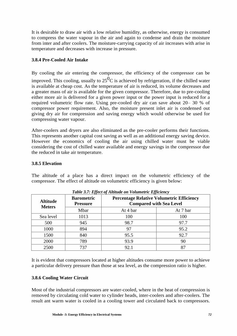
Module -3: Energy Efficiency in Electrical Systems 72
It is desirable to draw air with a low relative humidity, as otherwise, energy is consumed
to compress the water vapour in the air and again to condense and drain the moisture
from inter and after coolers. The moisture-carrying capacity of air increases with arise in
temperature and decreases with increase in pressure.
3.8.4 Pre-Cooled Air Intake
By cooling the air entering the compressor, the efficiency of the compressor can be
improved. This cooling, usually to 250C is achieved by refrigeration, if the chilled water
is available at cheap cost. As the temperature of air is reduced, its volume decreases and
a greater mass of air is available for the given compressor. Therefore, due to pre-cooling
either more air is delivered for a given power input or the power input is reduced for a
required volumetric flow rate. Using pre-cooled dry air can save about 20– 30 % of
compressor power requirement. Also, the moisture present inlet air is condensed out
giving dry air for compression and saving energy which would otherwise be used for
compressing water vapour.
After-coolers and dryers are also eliminated as the pre-cooler performs their functions.
This represents another capital cost saving as well as an additional energy saving device.
However the economics of cooling the air using chilled water must be viable
considering the cost of chilled water available and energy savings in the compressor due
the reduced in take air temperature.
3.8.5 Elevation
The altitude of a place has a direct impact on the volumetric efficiency of the
compressor. The effect of altitude on volumetric efficiency is given below:
Table 3.7: Effect of Altitude on Volumetric Efficiency
Altitude
Meters
Barometric
Pressure
Percentage Relative Volumetric Efficiency
Compared with Sea Level
Mbar At 4 bar At 7 bar
Sea level 1013 100 100
500 945 98.7 97.7
1000 894 97 95.2
1500 840 95.5 92.7
2000 789 93.9 90
2500 737 92.1 87
It is evident that compressors located at higher altitudes consume more power to achieve
a particular delivery pressure than those at sea level, as the compression ratio is higher.
3.8.6 Cooling Water Circuit
Most of the industrial compressors are water-cooled, where in the heat of compression is
removed by circulating cold water to cylinder heads, inter-coolers and after-coolers. The
result ant warm water is cooled in a cooling tower and circulated back to compressors.

Module -3: Energy Efficiency in Electrical Systems 73
The effect of cooling tower performance, total dissolved solids (TDS) in cooling water,
pumps and fans on compressor performance is discussed below:
Cooling Tower Performance
The main purpose of a cooling tower is to reduce the inlet warm water temperature to
near the wet bulb temperature of ambient air. Cooling towers are generally designed to
have an approach temperature of 2 to 5oC depending upon the type of cooling tower. In
practice, because of microbial growth, scale formation, corrosion and improper
maintenance, the intimate contact between air and water is disturbed, resulting in high
temperature outlet water which will affect compressor inter cooler effectiveness and
compressor performance. Proper maintenance of cooling tower is very important to
achieve the desired approach temperature.
Effect of air wet bulb temperature on cooling tower performance
The cooling tower performance is affected by atmospheric conditions–particularly by
the wet bulb temperature of inlet air. In a given location, the wet bulb temperature
changes throughout the year, reaching its peak value only occasionally. It would,
therefore, be uneconomical to operate the tower designed on the basis of the maximum
wet bulb temperature. A compromise between peak and average conditions has to be
adopted. While designing or selecting a cooling tower, “5 %” wet bulb temperature is
used which is, the wet bulb temperature not exceeded more than 5% of the total number
of hours during summer months. This is estimated from the study of local
meteorological data.
Cooling Tower Pump
Cooling water is supplied to compressors through centrifugal pumps at a particular
pressure and flow rate. Any change in water flow rate or pressure will affect the
compressor performance. High efficiency pumps and motors have to be selected, as they
run continuously. Inter connecting pipelines, inter-coolers, and after-coolers have to be
selected or designed for minimum pressure drop. Generally pumps in a central
compressor house are over-designed for safety reasons, and are capable of catering to
more than one compressor. During lean seasons and night shift, only one or two
compressors are in operation but cooling water is circulated through even in idle
compressors. To avoid this waste of water supply, idle compressors should be closed or
a water pressures witch fixed in the water line so that compressor can be tripped off
whenever the cooling water pressure falls below a pre-set value.
Cooling Tower fans
Cooling tower fans are provided to facilitate more air through put thus increasing
cooling tower efficacy. A malfunction of fan will result in less air to water ratio, change
in air distribution pattern etc., which will affect the cooling tower performance. Hence,
proper fan maintenance and fan energy management has to be adopted for lower energy
consumption.

Module -3: Energy Efficiency in Electrical Systems 74
• Once the cooling water temperature approaches set temperature, the cooling tower fan
can be switched off or operated intermittently by providing a interlock between water
outlet temperature and fan operation.
• If two speed motors are used the cooling tower fan power requirement can be reduced
substantially, whenever the ambient wet bulb temperature decreases.
• Automatic variable pitch propeller type fans and inverter type devices can be
incorporated to permit variable fan speeds. These can track the cooling load for a
constant outlet water temperature.
• Heavy fan blades made up of metals can be replaced with light weight, and
aerodynamically designed blades such as FRP to reduce the initial torque required and
the power consumption.
• Speed control of cooling tower fans by fluid-coupling drives can decrease– power
consumption in motors.
Cooling Water TDS
In most of the installations, raw water with high TDS is used for compressor cooling.
Because of in adequate attention to water quality, the TDS levels may shoot up to
unacceptable levels, due to water loss through evaporation, drift and other entertainment
losses. This leads to increase of scaling in cylinder heads, inter-coolers and after-
coolers, which reduces heat exchanger efficacy and compressor capacity. The scaling in
compressor and inter connecting pipe lines not only reduce its effectiveness but also
increases pressures drop and thus, water pumping power.
Table 3.8: Effect of Scaling on Pressure Drop and Inner Pipe Diameter
Scaling Thickness
(mm)
Inside Diameter Reduced Pressure
Drop From (mm) To (mm)
0.4 64 63.2 6
0.8 64 62.4 14
1.2 64 61.6 21
4.7 64 54.6 134
Use of treated water or purging apportion of cooling water periodically can maintain
TDS levels within acceptable limits. It is better to maintain the water pH by addition of
chemicals, and avoid microbial growth by addition of fungicides and algaecides.
3.8.7 Efficacy of Inter and After Coolers
Inter-coolers are provided between successive stage sofa multi-stage compressor to cool
the air, reduce its specific volume and condense out excess water. This reduces the
power requirement in consecutive stages. Ideally, the temperature of the inlet air at each
stage of a multi-stage machine should be the same as it was at the first stage. This is
referred to as “perfect cooling”. But in actual practice, because of fouled heat
exchangers, due to scaling of dissolved solids in cooling water, the inlet air temperatures
at subsequent stages are higher than the normal levels resulting in higher power
consumption, as a larger volume is handled for the same duty.

Module -3: Energy Efficiency in Electrical Systems 75
Table 3.9: Effect of Inter-stage Cooling on Specific Power Consumption of a Reciprocating
Compressor
Details Imperfect
Cooling
Perfect
Cooling
Chilled Water
Cooling
1 Stage inlet temperature0C 21.1 21.1 21.1
2 Stage inlet temperature0C 26.6 21.1 15.5
Capacity(m3/min) 15.5 15.6 15.7
Shaft Power (kW) 76.3 75.3 74.2
Specific energy consumption kW (m3/min) 4.9 4.8 4.7
Percent Change + 2.1 - - 2.1
It can be seen from the table 3.9 that an increase of 5.50C in the inlet to the second stage
results in a 2% increase in the specific energy consumption. Use of cold water reduces
power consumption. However, use of very cold water could result in condensation of
moisture in the air leading to cylinder damage. An after-cooler is located after the final
stage of the compressor to reduce air temperature and water content, as far as possible,
before air enters the receiver. As time passes, dissolved solids in the cooling water coat
the after-coolers, thereby reducing the heat transfer effectiveness. So, fouled after-
coolers, allow warm, humid air in to the receiver, which causes more condensation in air
receivers and distribution lines, which inconsequence, leads to increased corrosion.
Periodic cleaning of both heat exchangers and cylinder heads are therefore necessary.
Table 3.10: Table: Cooling Water Requirement
Compressor Type Minimum quantity of Cooling Water required for
2.85 m3/min. FAD at 7 bar (lpm)
Single-stage 3.8
Two-stage 7.6
Single-stage with after- cooler 15.1
Two-stage with after- cooler 18.9
Inter-cooler and after-cooler efficacy also depends upon the quantity of cooling water
circulated through the heat exchanger.
3.8.8 Pressure Settings
Reducing Delivery Pressure:
The power consumed by a compressor depends on its operating pressure and rated
capacity. They should not be operated above their optimum operating pressures as this
not only wastes energy, but also leads to excessive wear, leading to further energy
wastage. The volumetric efficiency of a compressor is also less at higher delivery
pressures. The possibility of down setting the delivery pressure should be explored by
careful study of pressure requirements of various equipment, and the pressure drop in
the line between the compressed air generation and utilization points. The pressure

Module -3: Energy Efficiency in Electrical Systems 76
switches must be adjusted such that the compressor cut-in and cuts-off at optimum
levels.
Table 3.11: Table: Power Reduction through Pressure Reduction
Pressure Reduction Power Reduction (%)
From(bar) To (bar) Single-stage
Water-cooled
Two-stage
Water-cooled
Two-stage Air-
cooled 6.8
6.8
6.1
5.5
4
9
4
11
2.6
6.5
A reduction in the delivery pressure of a compressor would reduce the power
consumption. This has been practically achieved, as discussed in the relevant case study.
Compressor modulation by Optimum Pressure Settings
Very often in an industry, different types, capacities and makes of compressors are
connected to a common distribution network. In such situations, proper selection of a
right combination of compressors and optimal modulation of different compressors can
conserve energy. Where more than one compressor feeds a common header,
compressors have to be operated in such a way that the cost of compressed air
generation is minimal.
If all compressors are similar, the pressure setting can be adjusted such that only one
compressor handles the load variation, whereas the others operate more or less at full
load.
If compressors are of different sizes, the pressure switch should be set such that only the
smallest compressor is allowed to modulate. If different types are operated together, for
example, both reciprocating and screw compressors, the reciprocating compressor must
be allowed to modulate, while keeping the screw compressor at full load always as its
part load operation consumes more power. In general, the compressor with lower no-
load power consumption must be modulated. Compress or scan be graded according to
their specific energy consumption, at different pressures and energy efficient ones must
be made to meet most of the demand.
Table 3.12: Expected Specific Power Consumption of Reciprocating Compressors (based on motor
input)
Pressure bar No. of Stages Specific Power kW/170 CMH
1 1 6.29
2 1 9.64
3 1 13.04
4 2 14.57
7 2 18.34
8 2 19.16
10 2 21.74
15 2 26.22

Module -3: Energy Efficiency in Electrical Systems 77
Mains air pressure reduction
It is often necessary to reduce the mains pressure when supply groups of plants or
complete workshops. This requires a pressure reducing valve of large capacity and good
flow characteristics. In these circumstances, a pressure reducing station may be used.
If the low pressure air requirement is considerable, it is advisable to generate low
pressure and high pressure air separately, and feed to the respective sections instead of
reducing the pressure through pressure reducing valves, which invariably waste energy.
Minimum pressure drop in air lines
The air mains and their associated branches, hoses, couplings and other accessories offer
considerable opportunities for energy conservation.
Table 3.13: Energy Wastage due to Smaller Pipe Diameter
Pipe Nominal Bore (mm) Pressure drop (bar) per
100meters
Equivalent power losses
(kW)
40 1.80 9.5
50 0.65 3.4
65 0.22 1.2
80 0.04 0.2
100 0.02 0.1
Excess pressure drop due to inadequate pipe sizing, choked filter elements, improperly
sized couplings and hoses represent energy wastage. The above table illustrates the
energy wastage, if the pipes are of smaller diameter.
Equivalent lengths of fittings
When long runs of distribution mains are involved, the pressure drops maybe higher
than acceptable levels; in such cases it is desirable to check for actual pressure drops.
Table 3.14: Resistance of Pipe Fittings in Equivalent Lengths (in metres)
Type of Fitting Nominal Pipe Size in mm
15 20 25 32 40 50 65 80 100 125
Gate Valve 0.11 0.14 0.18 0.27 0.32 0.40 0.49 0.64 0.91 1.20
Runof standard 0.12 0.18 0.24 0.38 0.40 0.52 0.67 0.85 1.20 1.52
Tee 90o long bend 0.15 0.18 0.24 0.38 0.46 0.61 0.76 0.91 1.20 1.52
Elbow 0.26 0.37 0.49 0.67 0.76 1.07 1.37 1.83 2.44 3.20

Module -3: Energy Efficiency in Electrical Systems 78
Return bend 0.46 0.61 0.76 1.07 1.20 1.68 1.98 2.60 3.66 4.88
Through side 0.52 0.70 0.91 1.37 1.58 2.14 2.74 3.66 4.88 6.40
Outlet of tee globe
valve 0.76 1.07 1.37 1.98 2.44 3.36 3.96 5.18 7.32 9.45
3.8.9 Blowers in place of Compressed Air System
Since the compressed air system is already available, facilities engineers may be
tempted to use compressed air to provide air for low pressure requirements such as
agitating plating tanks or pneumatic conveying. Using a blower that is designed for
lower pressure operation will cost only a fraction of compressed air generation cost.
3.8.10 Capacity Control of Compressors
In many installations, the use of air is intermittent. Therefore, some means of controlling
the output of the compressor is necessary. This is achieved by regulation of pressure,
volume, temperature or some other factors. The type of capacity control employed has a
direct impact on the compressor power consumption. Some control schemes commonly
used are discussed below:
On / Off Control
Automatic start and stop control, as its name implies, starts or stops the compressor by
means of a pressure activated switch as the air demand varies. This is a very efficient
method in controlling the capacity of compressor, where the motor idle-running losses
are eliminated, as it completely switches off the motor when the set pressure is reached.
This is suitable for small compressors (less than 10 kW).
Load and Unload
This is a two-step control where compressor is loaded when there is air demand and
unloaded when there is no air demand. During unload, the reciprocating compressor
motor runs without air compression, thereby consuming only 20- 30% of the full load
power. In screw compressors, the unloading is achieved by closing the inlet valve. The
idling power is about 40 to 50 % of the full load power depending configuration,
operation and maintenance practices. While in screw compressors, the unload power
consumption is marginally higher compared to reciprocating machines.
Multi-step Control
Motor-driven reciprocating compressors above75 kW are usually equipped with a multi-
step control. In this type of control, unloading is accomplished in a series of steps,
varying from full load down to no-load. A relevant case study has been appended for
this opportunity.

Module -3: Energy Efficiency in Electrical Systems 79
Table 3.15: Power Consumption of Reciprocating Compressor at Various Loads
Load % Power Consumption as % of full load Power
100 100 75 76-77 50 52-53 25 27-29 0 10-12
Five-step control (0%, 25%, 50%, 75% & 100%) is accomplished by means of clearance
pockets. In some cases, a movable cylinder head is provided for variable clearance in
the cylinder.
Throttling Control
This kind of control is achieved using an inlet valve or a variable–displacement slide
valve and is suitable for screw compressors where the capacity can be varied from 40 to
100%. The variable displacement method reduces the volume of air delivered by
venting air from a variable portion of the helical screw length to the inlet side of the
compressor. The variable displacement method is more efficient than the inlet valve.
The output of centrifugal compressors can be controlled using variable inlet guide vanes
to throttle discharge pressure. However, another efficient way to match compress or
output to meet varying load requirements is by speed control.
Table 3.16: Typical part load gas compression: Power input for speed and vane control of
centrifugal compressors
System Volume Flow % Speed Control Power Input (%) Vane Control
111 120 -
100 100 100
80 76 81
60 59 64
40 55 50
20 51 46
0 47 43
At low volumetric flow (below 40 %), vane control may result in lower power input
compared to speed control due to low efficiency of the speed control system. For loads
more than 40%, speed control is recommended.

Module -3: Energy Efficiency in Electrical Systems 80
3.8.11 Avoiding Misuse of Compressed Air
Misuse of compressed air for purposes like body cleaning, liquid agitation, floor
cleaning, drying, equipment cooling and other similar uses must be discouraged.
Wherever possible, low-pressure air from a blower should be substituted from
compressed air, for example secondary air for combustion in a boiler / furnace.
The following illustrations gives an idea of savings by stopping use of compressed air
by choosing alternative methods to perform the same task.
Electric motors can serve more efficiently than air-driven rotary devices. The following
table gives the comparison of pneumatic grinders and electrical grinders. Refer table
3.17 below:
Table 3.17: Power Requirements for Pneumatic and Electrical Tools
Tool Wheel dia
(mm) Speed (rpm)
Air Cons.
(m3/h) Power (kW)
Pneumatic angle grinder 150 6000 102 m3/h
at 6 bar 10.2
Electric angle grinder 150 5700-8600 N.A. 1.95 –2.90
Pneumatic jet grinder 35 30000 32.3 m3/h at 6
bar 3.59
Electric straight grinder 25 22900-30500 N.A. 0.18
It may be noted that in some area s use of electric tools are not permitted due to safety
constraints, especially places where inflammable vapours are present in the
environment. In those cases, possibility of shifting the machine tool operation to outside
the flammable area may be considered when evaluating use of electric tools. It should
always be remembered that safety consideration always overrides energy conservation.
In place of pneumatic hoists, electric hoists can be used. A comparison is given below:
Table 3.18: Comparison of Power Consumption of Pneumatic and Electric Hoists
Capacity Type
Compressed Air
Required
CMH
Equivalent Power
Consumption at the
Compressor, kW
Motor Rating of
an Electric
Hoist, kW
0.5 Chain 125 12 0.37
1.0 Chain 118 12 0.37
1.5 Chain 118 12 1.125
2 Chain 118 12 1.5
5 Wire rope 200 20.25 2.7
• Material conveying applications can be replaced by blower systems of
preferably by a combination of belt/ screw conveyers and bucket elevators. In

Module -3: Energy Efficiency in Electrical Systems 81
a paper manufacturing facility, compressed air was used for conveying wood
chips.
• For applications like blowing of components, use of compressed air
amplifiers, blowers or gravity-based systems may be possible. Brushes can
sweep away debris from work in progress as effectively as high-pressure air.
Blowers also can be used for this purpose. When moving air really is required
for an application, often sources other than compressed air can do the job.
Many applications do not require clean, dry, high-pressure and expensive 6
bar or 7 bar compressed air rather, only moving air is needed to blow away
debris, provide cooling, or other functions. In these cases, local air fans or
blowers may satisfy the need for moving air much economically.
• Use of compressed air for cleaning should be discouraged; use of vacuum
cleaners is an alternative for some applications. If absolutely necessary,
compressed air should be used only with blow guns to keep the air pressure
below 2 bar; higher pressure are not permitted as printer national safety
regulations. Use of compressed air amplifiers can also be considered for some
cleaning applications.
• For applications where compressed air is indispensable for cleaning internal
crevices of machines etc., installation of a separate cleaning air header with a
main isolation valve may be considered. The main valve should be opened
only for a few, well-defined time periods during the whole day, no
connections for cleaning should be provided from process or equipment air
lines.
• Replacement of pneumatically operated air cylinders by hydraulic power
packs can be considered.
• Use of compressed air for personal comfort cooling can cause grievous
injuries and is extremely wasteful; it should be banned from the safety
viewpoint alone. Use of man coolers or air washers (in dry areas) may be
encouraged. If a ¼” hosepipe is kept open ata 7 bar compressed air line for
personal cooling for at least 1000 hours/ annum, it can cost about 1,00,000
BDT/ annum.
• Vacuum systems are much more efficient than expensive venture methods,
which use expensive compressed air rushing past an orifice to create a
vacuum.
• Mechanical stirrers, conveyers, and low-pressure air many mix materials far
more economically than high-pressure compressed air.
3.8.12 Avoiding Air Leaks and Energy Wastage
The major opportunity to save energy is in the prevention of leaks in the compressed air
system. Leaks frequently occur at air receivers, relief valves, pipe and hose joints,
shutoff valves, quick release couplings, tools and equipment. In most cases, they are due
to poor maintenance and sometimes, improper installation in underground lines.

Module -3: Energy Efficiency in Electrical Systems 82
Air leakages through Different Size Orifices
The following table gives the amount of free air wasted for different nozzles sizes and
pressure:
Table 3.19: Discharge of Air through Orifice (Cd –1.0)
Gauge Pressure
Bar 0.5mm 1mm 2mm 3mm 5mm 10mm 12.5mm
0.5 0.06 0.22 0.92 2.1 5.7 22.8 35.5
1.0 0.08 0.33 1.33 3.0 8.4 33.6 52.5
2.5 0.14 0.58 2.33 5.5 14.6 58.6 91.4
5.0 0.25 0.97 3.92 8.8 24.4 97.5 152.0
7.0 0.33 1.31 5.19 11.6 32.5 129.0 202.0
Cost of Compressed Air Leakage
It may be seen from the following table that any expenditure on sealing leaks would be
paid back through energy saving.
Table 3.20: Cost of Air Leakage
Orifice Size mm KW Wasted * Energy Waste (BDT/Year)
0.8 0.2 8000
1.6 0.8 32000
3.1 3.0 120000
6.4 12.0 480000
* based on BDT 5 / kWh; 8000 operating hours; air at 7.0bar
Steps in simple shop-floor method for leak quantification
• Shut off compressed air operated equipment (or conduct test when no
equipment is using compressed air).
• Run the compressor to charge the system to set pressure of operation
• Note the sub-sequent time taken for ‘on load’ and ‘off load’ cycles of the
compressors. For accuracy, take ON & OFF times for 8 – 10 cycles
continuously. Then calculate total ‘ON’ Time (T) and Total ‘OFF’ time (t).
• The system leakage is calculated as
System leakage (m3/min) = Q × T / (T + t)
Q = Actual free air being supplied during trial, in cubic meters per minute
T = Time on load in minutes
t = Time unload in minutes

Module -3: Energy Efficiency in Electrical Systems 83
Example 3.1
Leakage Test by Ultrasonic Leak Detector
Leakage tests are conducted by a Leak Detector having a sensing probe, which senses
when there are leakages. The leak is detected by ultrasonic vibration. Leak testing is
done by observing and locating sources of ultrasonic vibrations created by turbulent
flow of gases passing through leaks in pressurized ore vacated systems. Use is made of
ultrasonic detector store veal air borne and structure-borne vibrations, and translators
that convert these in audible high frequency sounds to lower frequencies within the
range of human
hearing.Detectionofleaksincompressedairandgassystemsathightemperatures, beneath
insulated coverings, and in pipelines and manifolds, can be done.
Leak detection and location from a distance through air or other fluids involves remote
scanning of suspected leak areas with a directional probe and coordinating the direction
of the source of the characteristic hissing sound of the leak with the relative sound
intensity. Probably the greatest advantage of ultrasonic leak detection is that this method
can be used with any fluid (liquid, gas or vapour) if the physical conditions for sound
generation are met in the leak. When leak conditions generate sound in ambient air,
leaks can be detected up to and beyond 30 met (100feet). This offers advantages when
extended structures are to be inspected. Ultrasonic mechanical vibration signal energy,
is converted to electrical signal energy by an appropriate transducer. The single most
significant actor to be noted is the frequency distribution of ultrasonic energy from

Module -3: Energy Efficiency in Electrical Systems 84
leaks. All leaks possess energy in the30/50 kHz. At lower pressure of 480 and 70 kPa
(70and10psi), it is seen that there is a distinct maximum around 40 kHz.
3.8.13 Compressor Capacity Assessment
Need for Capacity Assessment
The compressor capacity is expressed in terms of quantity of free air delivered at a
particular pressure. Due to ageing of the compressors and inherent inefficiencies in the
internal components, the free air delivered may be less than the design value, despite
adherence to good maintenance practices. Sometimes, other factors such as poor
maintenance, fouled heat exchanger and effects of altitude also tend to reduce free air
delivery. In order to meet the air demand, the inefficient compressor may have to run for
more time, thus consuming more power than actually required.
The power wastage depends on the percentage deviation of FAD capacity. For example,
a worn out compressor valve can reduce the compressor capacity by as much as 20
percent. A periodic assessment of the FAD capacity of each compressor has to be
carried out to check its actual capacity. If the deviations are more than10%, corrective
measures should be taken to rectify the same.
The ideal method of compressor capacity assessment is through a nozzle test where in a
calibrated nozzle is used as a load, to vent out the generated compressed air. Flow is
assessed, based on the air temperature, stabilization pressure, orifice constant etc.
Simple method of Capacity Assessment in Shop-floor
• Isolate the compressor along with its individual
• Receiver being taken for test from main compressed air system by tightly
closing the isolation valve or blank, thus closing the receiver outlet.
• Open water drain valve and drain out water fully and empty the receiver and
the pipe line. Make sure that water trap is tightly closed once again to start the
test.
• Start the compressor and activate the stop watch.
• Note the time taken to attain the normal operational pressure P2 (in the
receiver) from initial pressure P1.
• Calculate the capacity as per the formulae given below:
Actual Free air discharge
P2 = Final pressure after filling (kg/cm2
a)
P1 = Initial pressure (kg/cm2a) after bleeding
P0 = Atmospheric Pressure (kg/cm2a)
V = Storage volume in m3
which includes receiver, after cooler, and delivery piping
T = Time take to build up pressure to P2 in minutes

Module -3: Energy Efficiency in Electrical Systems 85
Example 3.2
An instrument air compressor capacity test gave the following results – Comment?
Make: ABC
Date: ……………..
Time: ……………..
Test No.:1
Piston displacement: 16.88 CMM
Theoretical compressor capacity: 14.75 CMM @ 7 kg/SQCMG
Compressor rated rpm 750: Motor rated rpm1445
Receiver Volume: 7.79 CM
Additional hold up volume,
i.e., pipe / water cooler, etc., is: 0.4974 CM Total volume: 8.322CM
Initial pressure P1: 0.5 Kgf /SQCMG
Final pressure P2: 7.03 Kgf / SQCMG
Pump up time: 4.021-----
Atmospheric pressure P0: 1.026Kgf/cm2
a
Compressor output CMM =(P2 − P1) ∗ Total Volume
Atm. Pressure ∗ Pumpup time
(7.03 − 0.5) ∗ 8.322
1.026 ∗ 4.021= 13.17 CMM
Comment:
Capacityshortfallw.r.t.14.75CMMratingis1.577CMMi.e.,10.69%Compressor
performance needs to be investigated further.
Example 3.3
Assessing compressed air system study for a plant section gave following results.
Compressors on line A, B, C, D, E
• All reciprocating type
• Trial observation Summary
Compressor
Reference
Measured Capacity CMM
(@ 7 kgf/ SQCMG)
‘On’
Load kW
‘Unload’
kW
Load Time
Min.
Unload Time
Min.

Module -3: Energy Efficiency in Electrical Systems 86
A B C D E
13.17
12.32
13.14
12.75
13.65
115.30
117.20
108.30
104.30
109.30
42.3
51.8
43.3
29.8
39.3
Full time*
Full time*
Full time*
Full time*
5.88
0
0
0
0
39.12
*Compressors running in load conditions and not getting unloaded during normal
operations
Comments:
For a cycle time of 45 minutes (39.12 + 5.88)
i. Compressed air generated in M3
45 (13.17) + 45 (12.32) + 45 (13.14) + 45 (12.75) + 5.88 (13.65) =2392.36
ii. Power consumption kWh
45/60 (115.3) + 45/60 (117.20) + 45 / 60 (108.3) + 45/60 (104.3) + 5.88/60 (109.8)+
((39.12) / 60) 39.3 = 370.21kWh
iii. Compressed air generation capacity on line in M3
45 [13.17 + 12.32 + 13.14 + 12.75 + 13.65 ] = 2926.35M3
a) The consumption rate of the section connected
2392.36 / 45 CMM = 53.16 CMM
b) Compressor air draw las a % of capacity on line is [2392.36 / 2926.35 ] × 100 =
81.75%
c) Specific power consumption = 370.21 kWh / 2392.36 = 0.155
d) Idlepowerconsumptionduetounloadoperation=25.62kWhinevery45minutes cycle
i.e., 34.16 kWh every hour.
e) Itwouldbefavorableandenergyefficienttokeepthecompressor‘D’incyclingmode on
account of lower un-load losses.
f) A suitable smaller capacity compressor can be planned to replace the compressor
with highest unload losses.
g) An investigation is called for, as to why such a large variation of unload power
drawn, exists although all compressors have almost the same rated capacity.
3.8.14 Line Moisture Separator and Traps
Although, in an ideal system, all cooling and condensing of air should be carried out
before the air leaves the receiver, this is not very often achieved in practice. The amount
of condensation, which takes place in the lines, depends on the efficiency of moisture
extraction before the air leaves the receiver and the temperature in the mains itself. In
general, the air main should be given a fall of not less than 1 min 100 min the direction
of air flow, and the distance between drainage points should not exceed 30m.
Drainage points should be provided using equal tees, as it assists in the separation for
water. Whenever a branch line is taken off from the main sit should leave at the top so
that any water in the main does not fall straight in to the plant equipment. Further, the
bottom of the falling pipe should also be drained.

Module -3: Energy Efficiency in Electrical Systems 87
3.8.15 Compressed Air Filter
Although some water, oil and dirt are removed by the separators and traps in the mains,
still some of it is always left, which is being carried over. Moreover, pipe systems
accumulate scale and other foreign matters, such as small pieces of gasket material,
jointing compounds and soon. Burnt compressor oil may also be carried over in pipe
work, and this, with other contaminants, forms a gum my substance. To remove these,
all of which are liable to have deleterious effects on pneumatic equipment, the air
should be filtered as near as possible to the point of use. Water and oil collected in the
filter sump must be drained off because, if its level is allowed to build up, then it is
forced through the filter element in to the very system it is designed to protect.
3.8.16 Regulators
In many instances, pneumatic operations are to be carried out at a lower pressure than
that of the main supply. For these applications, pressure regulators are required to
reduce the pressure to the required value and also to ensure that it remains reasonably
constant at the usage point. Pilot operated type regulators are energy efficient than
direct-acting and self- relieving regulators. In the self-relieving type, a small relief valve
is provided which allows excess air to bleed away, should the downs tream pressure
exceed the set value. It is suitable for applications where the control pressure has to be
varied periodically.
3.8.17 Lubricators
Where air is used to drive prime movers, cylinders and valves, they should be fitted with
a lubricator. Essentially, a lubricator is are savoir of oil and has been designed so that
when air is flowing, metered amount of oil is fed in mist form into the air stream. This
oil is carried with the motive air, to the point of use to lubricate all moving parts. All
lubricators require a certain minimum rate of air flow to induce oil into their stream.
Their design should be such that once the air flow is more than this minimum rate, they
gives at is factory lubrication without causing an excessive pressure drop. Light free-
fogging, lubricating oil with a high velocity index and without lead additives is suitable
for lubrication. The ratio of oil to air can be decided experimentally. A rough guide is,
one drop of oil per minute for every 5 dm3/s of free air at 5.5 bar pressure.
It is advisable to fix filters, regulators and lubricators as close as possible to the
equipment being served. Where lubricators are used to provide oil for linear actuators or
when the direction of air flow is reversed, the volume of pipe work between the
lubricator and cylinder should not exceed to 50 % of the volume of free air used by the
cylinder per stroke.
3.8.18 Air Dryers
There are certain applications where air must be free from moisture and have a lower
dew point. This calls for more sophisticated and expensive methods to lower the dew
point of compressed air. Three commonly peps of air dryers used are heat-less
(absorption), absorption and chiller dryers. They produce dry air with10oC–40oC dew
point, depending on the type of dryers.

Module -3: Energy Efficiency in Electrical Systems 88
Table 3.21: Moisture Content in Air
Dew point at Atmospheric Pressure (oC) Moisture Content (ppm)
0 3800
-5 2500
-10 1600
-20 685
-30 234
-40 80
-60 6.5
Table 3.22: Pressure Dew Point and Power Consumption Data for Dryers
Type of Dryer Atmospheric
Dew Point (oC) First Cost
Operating
Cost
Power Cons. For
1000 m3
/hr
Refrigeration -20 Low Low 2.9 kW
Desiccant regenerative (by
compressed air purging) -20 Low High 20.7 kW
Desiccant regenerative
(external or internal heating
with electrical or steam
heater, reduced or no
compressed air purging)
-40 Medium Medium 18.0 kW
Desiccant regenerative (using
heated low pressure air, no
compressed air loss)
-40
High
Low
12.0 kW
Desiccant regenerative (by
recovery of heat of
Compression from
compressed air)
-40 High Very low 0.8 kW
3.8.19 Air Receivers
The main purpose of a receiver is to act as a pulsation damper, allowing inter mitten
thigh demands for compressed air to be met from a small compressor set, resulting in
lesser energy consumption.
If receiver is sized too small for air demand, compressor will run for longer periods. By
improving the ability of storage to meet air demand, running time of the compressor is
minimised, thereby reducing energy usage as well as wear and tear. Compressed air
systems usually have one primary receiver and possibly few secondary receivers near
high intermittent air using equipment.
The air receiver should be generously sized to give a large cooling surface and even out
the pulsation in delivered air pressure from a reciprocating compressor. As per IS 7938-
1976, volume of air in receiver (in m3) should be 1/10th to 1/6th of the output in m3/min.

Module -3: Energy Efficiency in Electrical Systems 89
A simple formulae often quoted for air receiver size is to take a value equal to one
minute’s continuous output of the compressor. However, this should be considered
indicative of the minimum size of receiver. A better suggestion is to estimate the peak
air consumption likely and allow for the maximum pressure drop that is acceptable at
this peak load.
If peaks cannot be quantified, another approximation can be to size the receiver
volumetobe5%of the rated hourly free air output. Providing an air receiver n earth load
end, where there is sudden high demand lasting for a short period, would avoid the need
to provide extra capacity.
3.8.20 Capacity Utilisation
In many installations, the use of air is intermittent. This means the compressor will be
operated on low load or no load condition, which increases the specific power
consumption per unit of air generated. Hence, for optimum energy consumption, a
proper compressor capacity control should be selected. The nature of the control device
depends on the function to be regulated. Regulation of pressure, volume, temperature or
some of factor determines the type of regulation required and the type of the
compressor drive.

Module -3: Energy Efficiency in Electrical Systems 90
Chapter 4: FANS AND BLOWERS
4.1 Introduction
Fans and blowers provide air for ventilation and industrial process requirements. Fans
generate a pressure to move air (or gases) against a resistance caused by ducts, dampers,
or other components in a fan system. The fan rotor receives energy from a rotating shaft
and transmits it to the air.
Difference between Fans, Blowers and Compressors
Fans, blowers and compressors are differentiated by the method used to move the air,
and by the system pressure they must operate against. As per American Society of
Mechanical Engineers (ASME) the specific ratio - the ratio of the discharge pressure
over the suction pressure - is used for defining the fans, blowers and compressors (see
Table 5.1)
Table 4.1 Differences between Fans, Blower and Compressor
4.2 Fan Types
Fan and blower selection depends on the volume flow rate, pressure, type of material
handled, space limitations, and efficiency. Fan efficiencies differ from design to design
and also by types. Typical ranges of fan efficiencies are given in Table 5.2.
Fans fall into two general categories: centrifugal flow and axial flow.
In centrifugal flow, airflow changes direction twice - once when entering and second
when leaving (forward curved, backward curved or inclined, radial) (see Figure 5.1).
In axial flow, air enters and leaves the fan with no change in direction (propeller, tubeaxial,
vaneaxial) (see Figure 5.2).

Module -3: Energy Efficiency in Electrical Systems 91
Table 4.2 Fan Efficiencies
Figure 4.1 Centrifugal Fan Figure 4.2 Axial Fan
Centrifugal Fan: Types
The major types of centrifugal fan are: radial, forward curved and backward curved
(see Figure 5.3).
Radial fans are industrial workhorses because of their high static pressures (upto 1400
mm WC) and ability to handle heavily contaminated airstreams. Because of their simple
design, radial fans are well suited for high temperatures and medium blade tip speeds.
Forward-curved fans are used in clean environments and operate at lower temperatures.
They are well suited for low tip speed and high-airflow work - they are best suited for
moving large volumes of air against relatively low pressures.

Module -3: Energy Efficiency in Electrical Systems 92
Backward-inclined fans are more efficient than forward-curved fans. Backward-
inclined fans reach their peak power consumption and then power demand drops off well
within their useable airflow range. Backward-inclined fans are known as "non-overloading"
because changes in static pressure do not overload the motor.
Figure 4.3 Types of Centrifugal Fans
Axial Flow Fan: Types
The major types of axial flow fans are: tube axial, vane axial and propeller (see Figure
5.4.)
Tubeaxial fans have a wheel inside a cylindrical housing, with close clearance between blade
and housing to improve airflow efficiency. The wheel turn faster than propeller fans,
enabling operation under high-pressures 250 — 400 mm WC. The efficiency is up to 65%.
Vaneaxial fans are similar to tubeaxials, but with addition of guide vanes that improve
efficiency by directing and straightening the flow. As a result, they have a higher static
pressure with less dependence on the duct static pressure. Such fans are used generally
for pressures upto 500 mmWC. Vaneaxials are typically the most energy-efficient fans
available and should be used whenever possible.
Propeller fans usually run at low speeds and moderate temperatures. They experience a
large change in airflow with small changes in static pressure. They handle large volumes
of air at low pressure or free delivery. Propeller fans are often used indoors as exhaust fans.
Outdoor applications include air-cooled condensers and cooling towers. Efficiency is low —
approximately 50% or less.

Module -3: Energy Efficiency in Electrical Systems 93
Figure 4.4 Types of Radial Fans
The different types of fans, their characteristics and typical applications are given in
Table
4.3 Common Blower Types
Blowers can achieve much higher pressures than fans, as high as 1.20 kg/cm2. They are
also used to produce negative pressures for industrial vacuum systems. Major types are:
centrifugal blower and positive-displacement blower.
Centrifugal blowers look more like centrifugal pumps than fans. The impeller is typically
driven and rotates as fast as 15,000 rpm. In multi-stage blowers, air is accelerated as it
passes through each impeller. In single-stage blower, air does not take many turns, and
hence it is more efficient.
Centrifugal blowers typically operate against pressures of 0.35 to 0.70 kg/cm2, but can
achieve higher pressures. One characteristic is that airflow tends to drop drastically as
system pressure increases, which can be a disadvantage in material conveying systems that
depend on a steady air volume. Because of this, they are most often used in applications that
are not prone to clogging.

Module -3: Energy Efficiency in Electrical Systems 94
Table 4.3 Types of Fans, Characteristics, and Typical Applications
Positive-displacement blowers have rotors, which "trap" air and push it through housing.
Positive-displacement blowers provide a constant volume of air even if the system
pressure varies. They are especially suitable for applications prone to clogging, since they can
produce enough pressure - typically up to 1.25 kg/cm2 - to blow clogged materials free. They
turn much slower than centrifugal blowers (e.g. 3,600 rpm), and are often belt driven to
facilitate speed changes.
4.4 Fan Performance Evaluation and Efficient System Operation
System Characteristics
The term "system resistance" is used when referring to the static pressure. The system
resistance is the sum of static pressure losses in the system. The system resistance is a
function of the configuration of ducts, pickups, elbows and the pressure drops across
equipment-for example bag filter or cyclone.

Module -3: Energy Efficiency in Electrical Systems 95
The system resistance varies with the square of the volume of air flowing through the
system. For a given volume of air, the fan in a system with narrow ducts and multiple short
radius elbows is going to have to work harder to overcome a greater system resistance
than it would in a system with larger ducts and a minimum number of long radius turns.
Long narrow ducts with many bends and twists will require more energy to pull the air
through them. Consequently, for a given fan speed, the fan will be able to pull less air
through this system than through a short system with no elbows. Thus, the system resistance
increases substantially as the volume of air flowing through the system increases; square of
air flow.
Figure 4.5 System Characteristics
Conversely, resistance decreases as flow decreases. To determine what volume the fan
will produce, it is therefore necessary to know the system resistance characteristics.
In existing systems, the system resistance can be measured. In systems that have been
designed, but not built, the system resistance must be calculated. Typically a system
resistance curve (see Figure 5.5) is generated with for various flow rates on the x-axis
and the associated resistance on the y-axis.
Fan Characteristics
Fan characteristics can be represented in form of fan curve(s). The fan curve is a
performance curve for the particular fan under a specific set of conditions. The fan
curve is a graphical representation of a number of inter-related parameters. Typically a curve
will be developed for a given set of conditions usually including: fan volume, system static
pressure, fan speed, and brake horsepower required to drive the fan under the stated
conditions. Some fan curves will also include an efficiency curve so that a system designer
will know where on that curve the fan will be operating under the chosen conditions (see Figure
5.6). In the many curves shown in the Figure, the curve static pressure (SP) vs. flow is
especially important.
The intersection of the system curve and the static pressure curve defines the operating
point. When the system resistance changes, the operating point is also changes. Once the
operating point is fixed, the power required could be found by following a vertical line that
passes through the operating point to an intersection with the power (BHP) curve. A

Module -3: Energy Efficiency in Electrical Systems 96
horizontal line drawn through the intersection with the power curve will lead to the
required power on the right vertical axis. In the depicted curves, the fan efficiency curve
is also presented.
System Characteristics and Fan Curves
In any fan system, the resistance to air flow (pressure) increases when the flow of air is
increased. As mentioned before, it varies as the square of the flow. The pressure required by
a system over a range of flows can be determined and a "system performance curve" can be
developed (shown as SC) (see Figure 5.7).
This system curve can then be plotted on the fan curve to show the fan's actual operating
point at "A" where the two curves (N1 and SC1) intersect. This operating point is at air
flow Q1 delivered against pressure P1.
Figure 4.6 Fan Characteristics Curve by Manufacturer
A fan operates along a performance given by the manufacturer for a particular fan speed. (The
fan performance chart shows performance curves for a series of fan speeds.) At fan
speed N1, the fan will operate along the N1 performance curve as shown in Figure 5.7. The
fan's actual operating point on this curve will depend on the system resistance; fan's
operating point at "A" is flow (Q1) against pressure (P1).
Two methods can be used to reduce air flow from Q1 to Q2:
First method is to restrict the air flow by partially closing a damper in the system. This
action causes a new system performance curve (SC2) where the required pressure is greater
for any given air flow. The fan will now operate at "B" to provide the reduced air flow Q2
against higher pressure P2.

Module -3: Energy Efficiency in Electrical Systems 97
Second method to reduce air flow is by reducing the speed from N1 to N2, keeping the
damper fully open. The fan would operate at "C" to provide the same Q2 air flow, but at
a lower pressure P3.
Thus, reducing the fan speed is a much more efficient method to decrease airflow since
less power is required and less energy is consumed.
Figure 4.7 System Curve
Fan Laws
The fans operate under a predictable set of laws concerning speed, power and pressure.
A change in speed (RPM) of any fan will predictably change the pressure rise and
power necessary to operate it at the new RPM.

Module -3: Energy Efficiency in Electrical Systems 98
Where Q — Flow, SP — Static Pressure, kW — Power and N — Speed (RPM)
4.5 Fan Design and Selection Criteria
Precise determination of air-flow and required outlet pressure are most important in
proper selection of fan type and size. The air-flow required depends on the process
requirements; normally determined from heat transfer rates, or combustion air or flue gas
quantity to be handled. System pressure requirement is usually more difficult to compute or
predict. Detailed analysis should be carried out to determine pressure drop across the length,
bends, contractions and expansions in the ducting system, pressure drop across filters, drop
in branch lines, etc. These pressure drops should be added to any fixed pressure required
by the process (in the case of ventilation fans there is no fixed pressure requirement).
Frequently, a very conservative approach is adopted allocating large safety margins, resulting
in over-sized fans which operate at flow rates much below their design values and, consequently,
at very poor efficiency.
Once the system flow and pressure requirements are determined, the fan and impeller type are
then selected. For best results, values should be obtained from the manufacturer for
specific fans and impellers.
The choice of fan type for a given application depends on the magnitudes of required
flow and static pressure. For a given fan type, the selection of the appropriate impeller
depends additionally on rotational speed. Speed of operation varies with the application.
High speed small units are generally more economical because of their higher hydraulic
efficiency and relatively low cost. However, at low pressure ratios, large, low-speed units
are preferable.
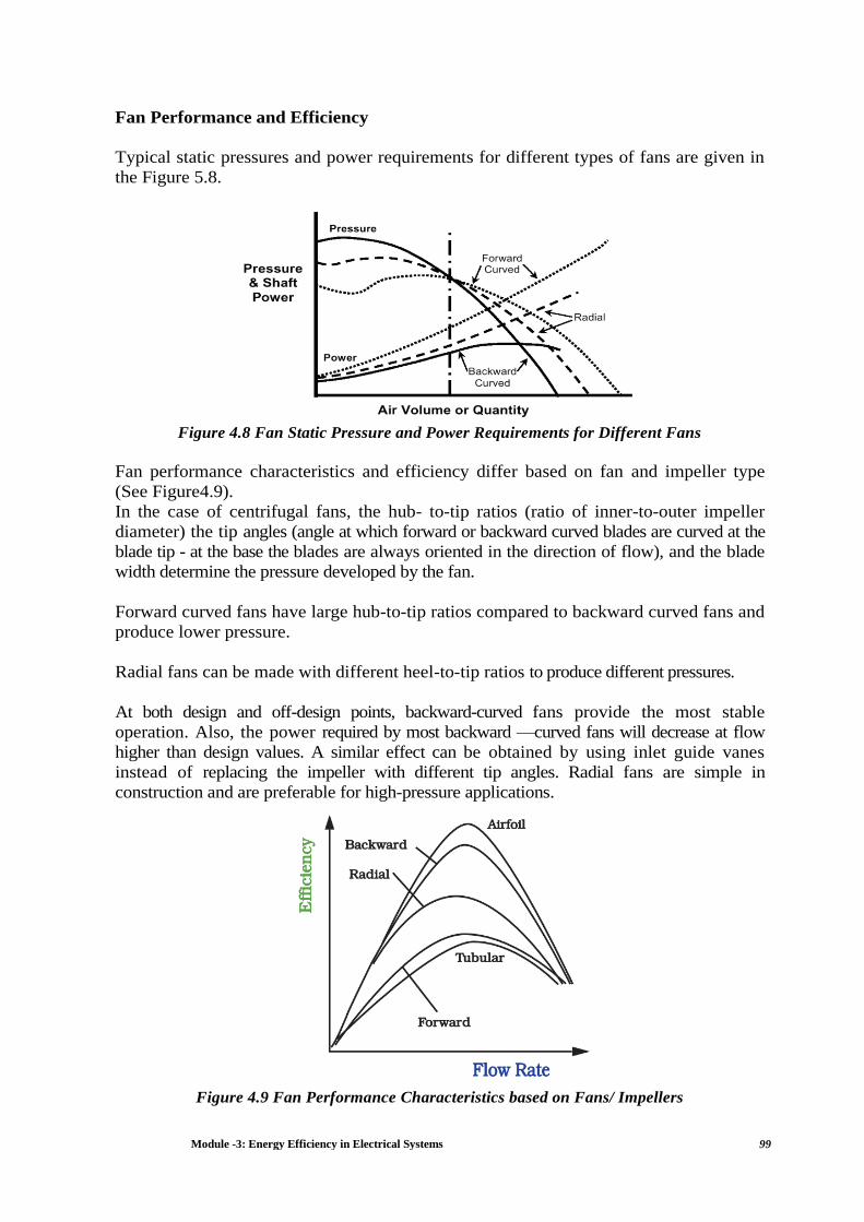
Module -3: Energy Efficiency in Electrical Systems 99
Fan Performance and Efficiency
Typical static pressures and power requirements for different types of fans are given in
the Figure 5.8.
Figure 4.8 Fan Static Pressure and Power Requirements for Different Fans
Fan performance characteristics and efficiency differ based on fan and impeller type
(See Figure4.9).
In the case of centrifugal fans, the hub- to-tip ratios (ratio of inner-to-outer impeller
diameter) the tip angles (angle at which forward or backward curved blades are curved at the
blade tip - at the base the blades are always oriented in the direction of flow), and the blade
width determine the pressure developed by the fan.
Forward curved fans have large hub-to-tip ratios compared to backward curved fans and
produce lower pressure.
Radial fans can be made with different heel-to-tip ratios to produce different pressures.
At both design and off-design points, backward-curved fans provide the most stable
operation. Also, the power required by most backward —curved fans will decrease at flow
higher than design values. A similar effect can be obtained by using inlet guide vanes
instead of replacing the impeller with different tip angles. Radial fans are simple in
construction and are preferable for high-pressure applications.
Figure 4.9 Fan Performance Characteristics based on Fans/ Impellers

Module -3: Energy Efficiency in Electrical Systems 100
Forward curved fans, however, are less efficient than backward curved fans and power
rises continuously with flow. Thus, they are generally more expensive to operate despite their
lower first cost.
Among centrifugal fan designs, aerofoil designs provide the highest efficiency (upto
10% higher than backward curved blades), but their use is limited to clean, dust-free air.
Axial-flow fans produce lower pressure than centrifugal fans, and exhibit a dip in pressure
before reaching the peak pressure point. Axial-flow fans equipped with adjustable / variable
pitch blades are also available to meet varying flow requirements.
Propeller-type fans are capable of high-flow rates at low pressures. Tube-axial fans have
medium pressure, high flow capability and are not equipped with guide vanes.
Vane-axial fans are equipped with inlet or outlet guide vanes, and are characterized by
high pressure, medium flow-rate capabilities.
Performance is also dependent on the fan enclosure and duct design. Spiral housing designs
with inducers, diffusers are more efficient as compared to square housings. Density of
inlet air is another important consideration, since it affects both volume flow-rate and
capacity of the fan to develop pressure. Inlet and outlet conditions (whirl and turbulence
created by grills, dampers, etc.) can significantly alter fan performance curves from that
provided by the manufacturer (which are developed under controlled conditions). Bends and
elbows in the inlet or outlet ducting can change the velocity of air, thereby changing fan
characteristics (the pressure drop in these elements is attributed to the system resistance).
All these factors, termed as System Effect Factors, should, therefore, be carefully
evaluated during fan selection since they would modify the fan performance curve.
Centrifugal fans are suitable for low to moderate flow at high pressures, while axial-
flow fans are suitable for low to high flows at low pressures. Centrifugal fans are generally
more expensive than axial fans. Fan prices vary widely based on the impeller type and the
mounting (direct-or-belt-coupled, wall-or-duct-mounted). Among centrifugal fans, aerofoil
and backward-curved blade designs tend to be somewhat more expensive than forward-
curved blade designs and will typically provide more favourable economics on a
lifecycle basis. Reliable cost comparisons are difficult since costs vary with a number of
application-specific factors. A careful technical and economic evaluation of available options is
important in identifying the fan that will minimize lifecycle costs in any specific
application.
Safety margin
The choice of safety margin also affects the efficient operation of the fan. In all cases
where the fan requirement is linked to the process/other equipment, the safety margin is to be
decided, based on the discussions with the process equipment supplier. In general, the safety
margin can be 5 % over the maximum requirement on flow rate.
In the case of boilers, the induced draft (ID) fan can be designed with a safety margin of
20 % on volume and 30 % on head. The forced draft (FD) fans and primary air (PA) fans do not
require any safety margins. However, safety margins of 10 % on volume and 20 % on
pressure are maintained for FD and PA fans.

Module -3: Energy Efficiency in Electrical Systems 101
Some pointers on fan specification
The right specification of the parameters of the fan at the initial stage, is pre-requisite
for choosing the appropriate and energy efficient fan.
The user should specify following information to fan manufacturer to enable right
selection: Design operating point of the fan — volume and pressure
Normal operating point - volume and pressure
Maximum continuous rating
Low load operation - This is particularly essential for units, which in the initial few years may
operate at lower capacities, with plans for upgradation at a later stage. The initial low
load and the later higher load operational requirements need to be specified clearly, so
that the manufacturer can supply a fan which can meet both the requirements, with different
sizes of impeller.
Ambient temperature — The ambient temperatures, both the minimum and maximum, are to
be specified to the supplier. This affects the choice of the material of construction of the
impeller
The maximum temperature of the gas at the fan during upset conditions should be specified to
the supplier This will enable choice of the right material of the required creep strength.
Density of gas at different temperatures at fan outlet
Composition of the gas — This is very important for choosing the material of
construction of the fan.
Dust concentration and nature of dust — The dust concentration and the nature of dust
(e.g. bagasse — soft dust, coal — hard dust) should be clearly specified.
The proposed control mechanisms that are going to be used for controlling the fan.
The operating frequency varies from plant-to-plant, depending on the source of power
supply. Since this has a direct effect on the speed of the fan, the frequency prevailing or
being maintained in the plant also needs to be specified to the supplier.
Altitude of the plant
The choice of speed of the fan can be best left to fan manufacturer. This will enable him
to design the fan of the highest possible efficiency. However, if the plant has some
preferred speeds on account of any operational need, the same can be communicated to the fan
supplier.
System Resistance and Pressure Drop
The system resistance has a major role in determining the performance and efficiency of a
fan. The system resistance also changes depending on the process. For example, the
formation of the coatings / erosion of the lining in the ducts, changes the system resistance
marginally. In some cases, the change of equipment (e.g. Replacement of Multi-cyclones with
ESP / Installation of low pressure drop cyclones in cement industry) duct modifications,
drastically shift the operating point, resulting in lower efficiency. In such cases, to maintain
the efficiency as before, the fan has to be changed.

Module -3: Energy Efficiency in Electrical Systems 102
Hence, the system resistance has to be periodically checked, more so when
modifications are introduced and action taken accordingly, for efficient operation of the
fan.
System resistance in the application of centrifugal fan is the resistance offered by all the
process equipment and duct line connected to the inlet of the fan as well as at the out let
of the fan, usually stacks. In the Figure 5.10 draft required to overcome the resistance
offered by the boiler to draw the flue gases -10 mmWc (- ve sign indicates the suction), the
draft required to draw the flue gases through the economiser, Air heater and dust control
system are added to estimate the total resistance at the inlet of the ID fan (i.e. -10 - 30 - 40 - 150
= - 230 mmWc). However the ID fan requires a minimum of 10 mmWc pressure to push the
gases to the bottom of the stack from where the gases will be taken care by natural draft
into atmosphere. Hence the overall resistance (pressure drop) to be build up by the ID fan
is the difference between the outlet pressure and the inlet pressure [i.e. 10 - (-230) = 240
mmWc].
Figure 4.10 Pressure Drop across Various Equipment
System resistance is a function of gas density and the velocity of the gas. In the Figure
5.10 initially when there is no flue gas generation, there is no gas velocity in the process
equipment and the ducts and hence the resistance (pressure drop) is zero (see Figure 5.11).
After the boiler firing is started, there is continuous increase in the generation of flue gases
and accordingly there is continuous increase in the velocity of the gases and continuous
increase in draft. When the boiler is fired at rated capacity, the generation of flue gases are
maximum resulting in corresponding pressure drop, which is the "operating point" (
30,000 m3/hr, 240 mmWc) of the boiler ( Figure 5.11). Accordingly the ID fan with a
characteristic (Performance) curve passing through the "operating point" of the system at the
highest possible fan efficiency has to be selected for better utilisation of energy.

Module -3: Energy Efficiency in Electrical Systems 103
Figure 4.11 Fan System Curve
4.6 Flow Control Strategies
Typically, once a fan system is designed and installed, the fan operates at a constant speed.
There may be occasions when a speed change is desirable, i.e., when adding a new run of
duct that requires an increase in air flow (volume) through the fan. There are also
instances when the fan is oversized and flow reductions are required.
Various ways to achieve change in flow are: pulley change, damper control, inlet guide
vane control, variable speed drive and series and parallel operation of fans.
Pulley Change
When a fan volume change is required on a permanent basis, and the existing fan can handle the
change in capacity, the volume change can be achieved with a speed change. The
simplest way to change the peed is with a pulley change. For this, the fan must be driven
by a motor through a v-belt system. The fan speed can be increased or decreased with a change in
the drive pulley or the driven pulley or in some cases, both pulleys. As shown in the Figure 5.12,
a higher sized fan operating with damper control was downsized by reducing the motor
(drive) pulley size from 8" to 6". The power reduction was 12 kW.

Module -3: Energy Efficiency in Electrical Systems 104
Figure 4.12 Pulley Change
Damper Controls
Some fans are designed with damper controls (see Figure 5.13). Dampers can be located
at inlet or outlet. Dampers provide a means of changing air volume by adding or
removing system resistance. This resistance forces the fan to move up or down along its
characteristic curve, generating more or less air without changing fan speed. However,
dampers provide a limited amount of adjustment, and they are not particularly energy
efficient.
Figure 4.13 Damper change

Module -3: Energy Efficiency in Electrical Systems 105
Inlet Guide Vanes
Inlet guide vanes are another mechanism that can be used to meet variable air demand (see Figure
5.14). Guide vanes are curved sections that lay against the inlet of the fan when they are open.
When they are closed, they extend out into the air stream. As they are closed, guide vanes pre-
swirl the air entering the fan housing. This changes the angle at which the air is presented to the fan
blades, which, in turn, changes the characteristics of the fan curve. Guide vanes are energy
efficient for modest flow reductions — from 100 percent flow to about 80 percent. Below 80
percent flow, energy efficiency drops sharply.
Figure 4.14 Inlet Guide Vanes
Axial-flow fans can be equipped with variable pitch blades, which can be hydraulically or
pneumatically controlled to change blade pitch, while the fan is at stationary. Variable-
pitch blades modify the fan characteristics substantially and thereby provide dramatically higher
energy efficiency than the other options discussed thus far.
Variable Speed Drives
Although, variable speed drives are expensive, they provide almost infinite variability in
speed control. Variable speed operation involves reducing the speed of the fan to meet
reduced flow requirements. Fan performance can be predicted at different speeds using the fan
laws. Since power input to the fan changes as the cube of the flow, this will usually be the most
efficient form of capacity control. However, variable speed control may not be economical for
systems, which have infrequent flow variations. When considering variable speed drive, the
efficiency of the control system (fluid coupling, eddy-current, VFD, etc.) should be accounted
for, in the analysis of power consumption.

Module -3: Energy Efficiency in Electrical Systems 106
Series and Parallel Operation
Parallel operation of fans is another useful form of capacity control. Fans in parallel can
be additionally equipped with dampers, variable inlet vanes, variable-pitch blades, or speed
controls to provide a high degree of flexibility and reliability.
Combining fans in series or parallel can achieve the desired airflow without greatly
increasing the system package size or fan diameter. Parallel operation is defined as having
two or more fans blowing together side by side.
Figure 4.15: Series and Parallel Operation
The performance of two fans in parallel will result in doubling the volume flow, but only at
free delivery. As Figure 5.15 shows, when a system curve is overlaid on the parallel
performance curves, the higher the system resistance, the less increase in flow results
with parallel fan operation. Thus, this type of application should only be used when the fans
can operate in a low resistance almost in a free delivery condition.
Series operation can be defined as using multiple fans in a push-pull arrangement. By staging
two fans in series, the static pressure capability at a given airflow can be increased, but
again, not to double at every flow point, as the above Figure displays. In series operation,
the best results are achieved in systems with high resistances.
In both series and parallel operation, particularly with multiple fans certain areas of the
combined performance curve will be unstable and should be avoided. This instability is
unpredictable and is a function of the fan and motor construction and the operating point.
Factors to be considered in the selection of flow control methods
Comparison on of various volume control methods with respect to power consumption
(%) required power is shown in Figure 4.16.

Module -3: Energy Efficiency in Electrical Systems 107
All methods of capacity control mentioned above have turn-down ratios (ratio of
maximum—to minimum flow rate) determined by the amount of leakage (slip) through
the control elements. For example, even with dampers fully closed, the flow may not be zero
due to leakage through the damper. In the case of variable-speed drives the turn-down ratio is
limited by the control system. In many cases, the minimum possible flow will be
determined by the characteristics of the fan itself. Stable operation of a fan requires that it
operate in a region where the system curve has a positive slope and the fan curve has a
negative slope.
The range of operation and the time duration at each operating point also serves as a
guide to selection of the most suitable capacity control system. Outlet damper control due to
its simplicity, ease of operation, and low investment cost, is the most prevalent form of
capacity control. However, it is the most inefficient of all methods and is best suited for
situations where only small, infrequent changes are required (for example, minor process
variations due to seasonal changes. The economic advantage of one method over the other
is determined by the time duration over which the fan operates at different operating points. The
frequency of flow change is another important determinant. For systems requiring frequent flow
control, damper adjustment may not be convenient. Indeed, in many plants, dampers are
not easily accessible and are left at some intermediate position to avoid frequent control.
Figure- 4.16: Comparison: Various Volume Control Methods
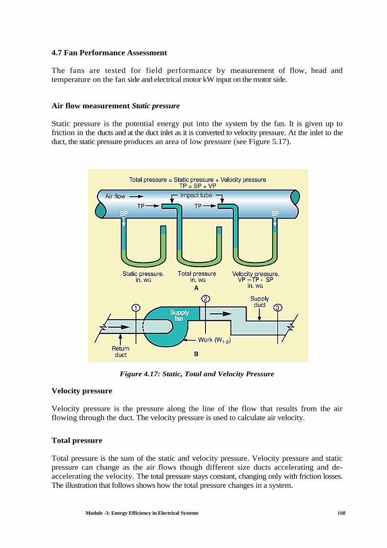
Module -3: Energy Efficiency in Electrical Systems 108
4.7 Fan Performance Assessment
The fans are tested for field performance by measurement of flow, head and
temperature on the fan side and electrical motor kW input on the motor side.
Air flow measurement Static pressure
Static pressure is the potential energy put into the system by the fan. It is given up to
friction in the ducts and at the duct inlet as it is converted to velocity pressure. At the inlet to the
duct, the static pressure produces an area of low pressure (see Figure 5.17).
Figure 4.17: Static, Total and Velocity Pressure
Velocity pressure
Velocity pressure is the pressure along the line of the flow that results from the air
flowing through the duct. The velocity pressure is used to calculate air velocity.
Total pressure
Total pressure is the sum of the static and velocity pressure. Velocity pressure and static
pressure can change as the air flows though different size ducts accelerating and de-
accelerating the velocity. The total pressure stays constant, changing only with friction losses.
The illustration that follows shows how the total pressure changes in a system.

Module -3: Energy Efficiency in Electrical Systems 109
The fan flow is measured using pitot tube manometer combination, or a flow sensor
(differential pressure instrument) or an accurate anemometer. Care needs to be taken regarding
number of traverse points, straight length section (to avoid turbulent flow regimes of
measurement) upstream and downstream of measurement location. The measurements can
be on the suction or discharge side of the fan and preferably both where feasible.
Measurement by Pitot tube
The Figure 5.18 shows how velocity pressure is measured using a pitot tube and a
manometer. Total pressure is measured using the inner tube of pitot tube and static pressure
is measured using the outer tube of pitot tube. When the inner and outer tube ends are
connected to a manometer, we get the velocity pressure. For measuring low velocities, it is
preferable to use an inclined tube manometer instead of U tube manometer.
Figure 4.18 Velocity Measurement Using Pitot Tube
Measurements and Calculations
Velocity pressure/velocity calculation
When measuring velocity pressure the duct diameter (or the circumference from which
to calculate the diameter) should be measured as well. This will allow us to calculate the
velocity and the volume of air in the duct. In most cases, velocity must be measured at several
places in the same system.
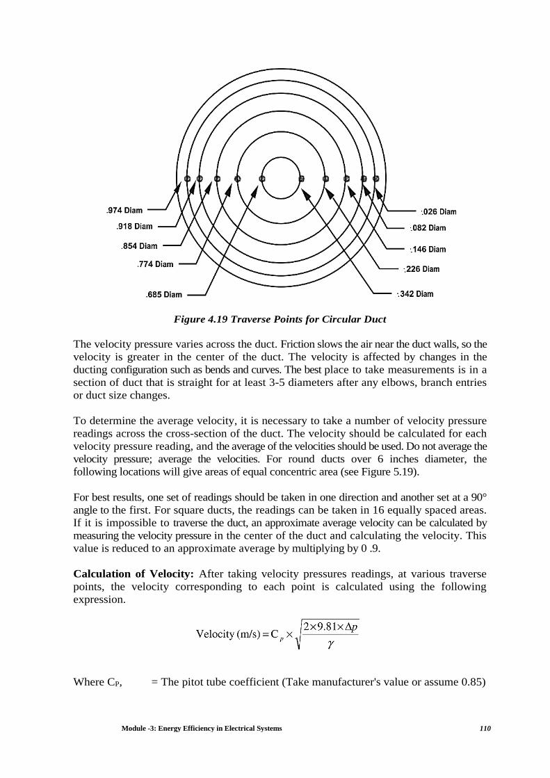
Module -3: Energy Efficiency in Electrical Systems 110
Figure 4.19 Traverse Points for Circular Duct
The velocity pressure varies across the duct. Friction slows the air near the duct walls, so the
velocity is greater in the center of the duct. The velocity is affected by changes in the
ducting configuration such as bends and curves. The best place to take measurements is in a
section of duct that is straight for at least 3-5 diameters after any elbows, branch entries
or duct size changes.
To determine the average velocity, it is necessary to take a number of velocity pressure
readings across the cross-section of the duct. The velocity should be calculated for each
velocity pressure reading, and the average of the velocities should be used. Do not average the
velocity pressure; average the velocities. For round ducts over 6 inches diameter, the
following locations will give areas of equal concentric area (see Figure 5.19).
For best results, one set of readings should be taken in one direction and another set at a 90°
angle to the first. For square ducts, the readings can be taken in 16 equally spaced areas.
If it is impossible to traverse the duct, an approximate average velocity can be calculated by
measuring the velocity pressure in the center of the duct and calculating the velocity. This
value is reduced to an approximate average by multiplying by 0 .9.
Calculation of Velocity: After taking velocity pressures readings, at various traverse
points, the velocity corresponding to each point is calculated using the following
expression.
Where CP, = The pitot tube coefficient (Take manufacturer's value or assume 0.85)

Module -3: Energy Efficiency in Electrical Systems 111
ΔP = The average velocity pressure measured using pitot tube and inclined
manometer by taking number of points over the entire cross-section of the duct, mm Water
Column
γ = Gas density at flow conditions, kg/m3
EXAMPLE 4.1
Air flow measurements using the pitot tube, in the primary air fan of a coal fired boiler
gave the following data, calculate the velocity of air.
Air temperature = 38°C
Velocity pressure = 47 mmWC
Pitot tube constant, Cp = 0.9
Air density at 38°C = 1.135 kg /m3
Find out the velocity of air in m/sec.
Calculation of gas density
To calculate the velocity and volume from the velocity pressure measurements, it is
necessary to know the density of gas. The density is dependent on altitude, temperature,
molecular weight and pressure.
Module -3: Energy Efficiency in Electrical Systems 112
Fan efficiency
Fan manufacturers generally use two ways to mention fan efficiency: mechanical efficiency
(sometimes called the total efficiency) and static efficiency. Both measure how well the
fan converts horsepower into flow and pressure.
The equation for determining mechanical efficiency is:
The static efficiency equation is the same except that the outlet velocity pressure is not
added to the fan static pressure
Drive motor kW can be measured by a load analyzer. This kW multiplied by motor
efficiency gives the shaft power to the fan.
4.8 Energy Savings Opportunities
Minimizing demands on the fan.
1. Minimising excess air level in combustion systems to reduce FD fan and ID fan
load.
2. Minimising air in-leaks in hot flue gas path to reduce ID fan load, especially in
case of kilns, boiler plants, furnaces, etc. Cold air in-leaks increase ID fan load
tremendously, due to density increase of flue gases and in-fact choke up the
capacity of fan, resulting as a bottleneck for boiler / furnace itself.
3. In-leaks / out-leaks in air conditioning systems also have a major impact on
energy efficiency and fan power consumption and need to be minimized.
The findings of performance assessment trials will automatically indicate potential areas
for improvement, which could be one or a more of the following:
1. Change of impeller by a high efficiency impeller along with cone.
2. Change of fan assembly as a whole, by a higher efficiency fan
3. Impeller derating (by a smaller dia impeller)
4. Change of metallic / Glass reinforced Plastic (GRP) impeller by the more energy
efficient hollow FRP impeller with aerofoil design, in case of axial flow fans, where
significant savings have been reported
5. Fan speed reduction by pulley dia modifications for derating
6. Option of two speed motors or variable speed drives for variable duty conditions
7. Option of energy efficient flat belts, or, cogged raw edged V belts, in place of
conventional V belt systems, for reducing transmission losses.
8. Adopting inlet guide vanes in place of discharge damper control
9. Minimizing system resistance and pressure drops by improvements in duct
system

Module -3: Energy Efficiency in Electrical Systems 113
4.9 Case Study on Pressure Drop Reduction Across the Bag Filter
One of the Cement filter bag house is experiencing high Differential Pressure (DP)
across the bag house while producing one particular type of cement. This high DP is
resulting in high power consumption and puffing from the bag house. Upon examination it has
been found that particle size distribution for this particular type of Cement associated with
the fineness is creating high DP.
The results of this replacement are self-explanatory in the details given below:
Application Bag Filter for Cement Mill
Problem High DP across the bag house while producing one
particular type of Cement Product
Reason for the Problem Characteristics of particle size distribution associated
with its fineness is creating high DP across the bag house
Solution Replace the existing filter bags with PTFE Membrane
filter bags
Results Reduction of 50mm WC in DP across the bag house
Reduction of 5kWh in power consumption
Existing Bag Bag with membrane
40000 41600
96.8/86.9 98.2/88.7
Mixed Felt
Mixed Felt with PTFE
membrane
165 115
51 46
Conclusion
The above results are categorically demonstrating that
by changing the filter fabric we can achieve
significant performance improvement of the bag house
Case Studies VSD Applications
Case 1: Cement plants use a large number of high capacity fans. By using liners on the
impellers, which can be replaced when they are eroded by the abrasive particles in the
dust-laden air, the plants have been able to switch from radial blades to forward-curved and
backward-curved centrifugal fans. This has vastly improved system efficiency without
requiring frequent impeller changes.
For example, a careful study of the clinker cooler fans at a cement plant showed that the
flow was much higher than required and also the old straight blade impeller resulted in
low system efficiency. It was decided to replace the impeller with a backward-curved
blade and use liners to prevent erosion of the blade. This simple measure resulted in a 53 %
reduction in power consumption, which amounted to annual savings of Rs. 2.1 million.
Case 2: Another cement plant found that a large primary air fan which was belt driven through
an arrangement of bearings was operating at system efficiency of 23 %. The fan was
replaced with a direct coupled fan with a more efficient impeller. Power consumption reduced
from 57 kW to 22 kW. Since cement plants use a large number of fans, it is generally possible
to integrate the system such that air can be supplied from a common duct in many cases.

Module -3: Energy Efficiency in Electrical Systems 114
For example, a study indicated that one of the fans was operated with the damper open
to only 5 %. By re-ducting to allow air to be supplied from another duct where flow was
being throttled, it was possible to totally eliminate the use of a 55 kW fan.
Case 3: The use of variable-speed drives for capacity control can result in significant
power savings. A 25 ton-per-hour capacity boiler was equipped with both an induced-draft and
forced-draft fan. Outlet dampers were used to control the airflow. After a study of the air-flow
pattern, it was decided to install a variable speed drive to control air flow. The average power
consumption was reduced by nearly 41 kW resulting in annual savings of Rs. 0.33 million. The
investment of Rs. 0.65 million for the variable-speed drive was paid back in under 2 years.
Case 4: The type of variable-speed drive employed also significantly impacts power
consumption. Thermal power stations install a hydraulic coupling to control the capacity
of the induced-draft fan. It was decided to install a VFD on ID fans in a 200 MW thermal
power plant. A comparison of the power consumption of the two fan systems indicated that
for similar operating conditions of flow and plant power generation, the unit equipped with the
VFD control unit consumed, on average, 4 million units / annum less than the unit equipped
with the hydraulic coupling.
4.10 Computational Fluid Dynamics
Use of Computational Fluid Dynamics (CFD) for Energy Efficiency
Computational Fluid Dynamics (CFD) is a powerful computer based simulation tool,
which uses mathematics to model the physical system and to solve equations to predict the mass,
momentum and energy. CFD tools helps to visualize the flow pattern, temperature and pressure
profiles as well as particle movement inside the equipment / system under consideration. Being a
simulation tool, various designs / operating parameters can be changed to arrive at best operating
conditions for the plant. This also helps to determine the effect of changes in key process
parameters before making any changes in the manufacturing process at plant. Since it is a
proactive analysis and design tool, it can highlight the root cause not just the effect when
evaluating plant problems. It is able to reduce scale-up problems because the models are based on
fundamental physics and are scale independent. It is also useful in simulating conditions where it is
not possible to take detailed measurements because of high temperature or dangerous
environment.
Application of CFD in a Fan System for Energy Efficiency
In addition to optimization of the fan itself, the upstream and downstream flow situations are
important for trouble free operation of the fan and maximum possible efficiency. If, for
instance, the incoming flow is turbulent or swirling because of poorly designed bends or
changes in cross-section, this will affect the fan's operating characteristics. Disturbances in the
inflow and outflow zones have particularly serious effects in the case of high efficiency fans
(> 80 %); as such fans depend on a non-swirling inflow in order to achieve their efficiency
figures.
This case study describes the optimization of the induced draught flow of a double-inlet fan
using CFD. Figure 4.20 shows the system arrangement drawing. The 3D model derived
from this drawing is shown in Figure 4.21. The very sharp-edged transitions at inlet side
affect the smooth flow.

Module -3: Energy Efficiency in Electrical Systems 115
Figure 4.20 System arrangement drawing with induced draught fan
Figure 4.21 3D model of induced draught fan
The simulation (Figure 4.22) shows extensive flow disruption and instability. The pressure
drop of this system is correspondingly high. From the inlet until the end of the first
branch, the pressure drop is about 260 Pa. From the inlet until the next branch the drop is as
high as 430 Pa because of the flow disruption near the end of the horizontal duct.

Module -3: Energy Efficiency in Electrical Systems 116
Figure 4.22 Total pressure profile with original design
Figure 4.23 Total pressure profile after optimizing design
The black circles indicate unfavourable situations because this design involves
transitions that are too sharp-edged and thus prevent the flow from following the contours,
resulting in turbulence. This causes pressure drops and thus leads to additional electrical energy
consumption. By contrast, the white circle indicates a duct end producing an inefficient fluid
flow.
Since a portion of the vortex flow is sucked into the fan it has to cope with strongly
swirling inflow air and therefore loses efficiency and suffers from mechanical
vibrations.
Optimization of the geometry involved redesigning the critical points highlighted in Figure
5.22 so that the cross-section transitions were smooth. This redesigning succeeded in
reducing the pressure drop at the front inflow duct to the fan by a factor of four, from
261 Pa to 66 Pa, while the pressure drop at the rear inflow duct that had been caused by the
poorly-designed horizontal duct end (Figure 5.22, white circle) was even reduced to little
more than one sixth the original figure. The severe swirling of the fan intake air (Figure
5.23, red circles) was also significantly reduced, enabling the fan to achieve its rated
performance figures.
The mean pressure drop saving of 275 Pa at a volume flow of 5,00,000 m3/h
significantly reduces the power consumption. The resultant power saving was of the order
of 49 kW.
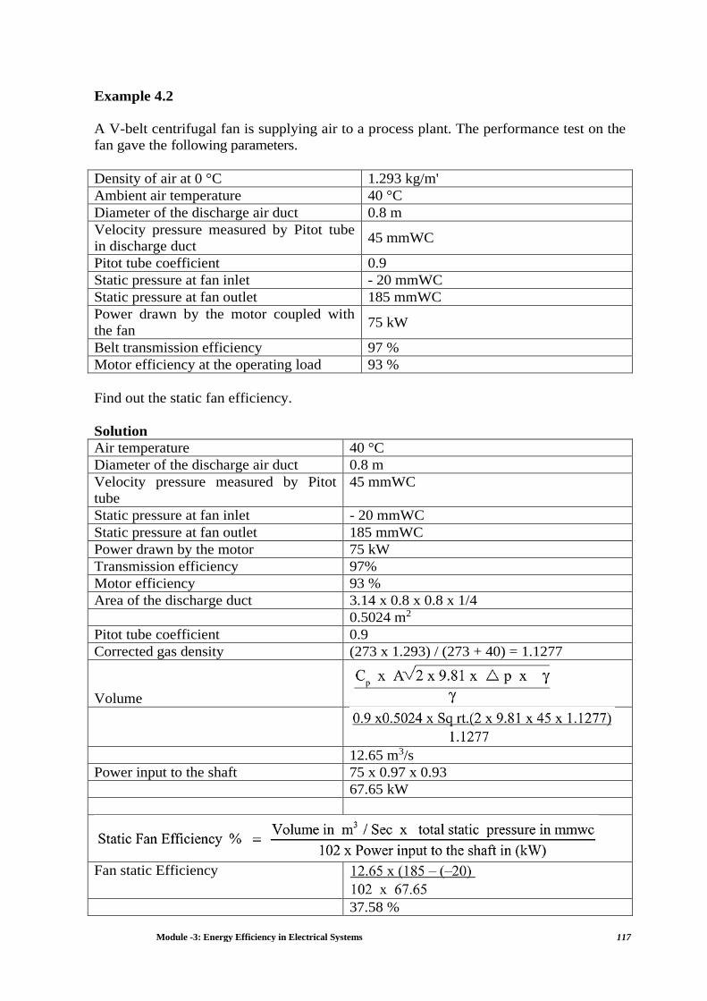
Module -3: Energy Efficiency in Electrical Systems 117
Example 4.2
A V-belt centrifugal fan is supplying air to a process plant. The performance test on the
fan gave the following parameters.
Density of air at 0 °C 1.293 kg/m'
Ambient air temperature 40 °C
Diameter of the discharge air duct 0.8 m
Velocity pressure measured by Pitot tube
in discharge duct 45 mmWC
Pitot tube coefficient 0.9
Static pressure at fan inlet - 20 mmWC
Static pressure at fan outlet 185 mmWC
Power drawn by the motor coupled with
the fan 75 kW
Belt transmission efficiency 97 %
Motor efficiency at the operating load 93 %
Find out the static fan efficiency.
Solution
Air temperature 40 °C
Diameter of the discharge air duct 0.8 m
Velocity pressure measured by Pitot
tube
45 mmWC
Static pressure at fan inlet - 20 mmWC
Static pressure at fan outlet 185 mmWC
Power drawn by the motor 75 kW
Transmission efficiency 97%
Motor efficiency 93 %
Area of the discharge duct 3.14 x 0.8 x 0.8 x 1/4
0.5024 m2
Pitot tube coefficient 0.9
Corrected gas density (273 x 1.293) / (273 + 40) = 1.1277
Volume
12.65 m3/s
Power input to the shaft 75 x 0.97 x 0.93
67.65 kW
Fan static Efficiency
37.58 %
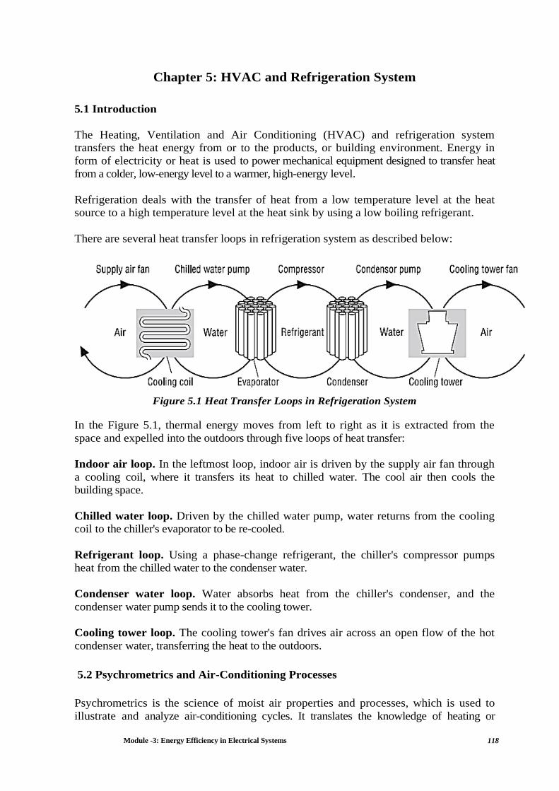
Module -3: Energy Efficiency in Electrical Systems 118
Chapter 5: HVAC and Refrigeration System
5.1 Introduction
The Heating, Ventilation and Air Conditioning (HVAC) and refrigeration system
transfers the heat energy from or to the products, or building environment. Energy in
form of electricity or heat is used to power mechanical equipment designed to transfer heat
from a colder, low-energy level to a warmer, high-energy level.
Refrigeration deals with the transfer of heat from a low temperature level at the heat
source to a high temperature level at the heat sink by using a low boiling refrigerant.
There are several heat transfer loops in refrigeration system as described below:
Figure 5.1 Heat Transfer Loops in Refrigeration System
In the Figure 5.1, thermal energy moves from left to right as it is extracted from the
space and expelled into the outdoors through five loops of heat transfer:
Indoor air loop. In the leftmost loop, indoor air is driven by the supply air fan through
a cooling coil, where it transfers its heat to chilled water. The cool air then cools the
building space.
Chilled water loop. Driven by the chilled water pump, water returns from the cooling
coil to the chiller's evaporator to be re-cooled.
Refrigerant loop. Using a phase-change refrigerant, the chiller's compressor pumps
heat from the chilled water to the condenser water.
Condenser water loop. Water absorbs heat from the chiller's condenser, and the
condenser water pump sends it to the cooling tower.
Cooling tower loop. The cooling tower's fan drives air across an open flow of the hot
condenser water, transferring the heat to the outdoors.
5.2 Psychrometrics and Air-Conditioning Processes
Psychrometrics is the science of moist air properties and processes, which is used to
illustrate and analyze air-conditioning cycles. It translates the knowledge of heating or
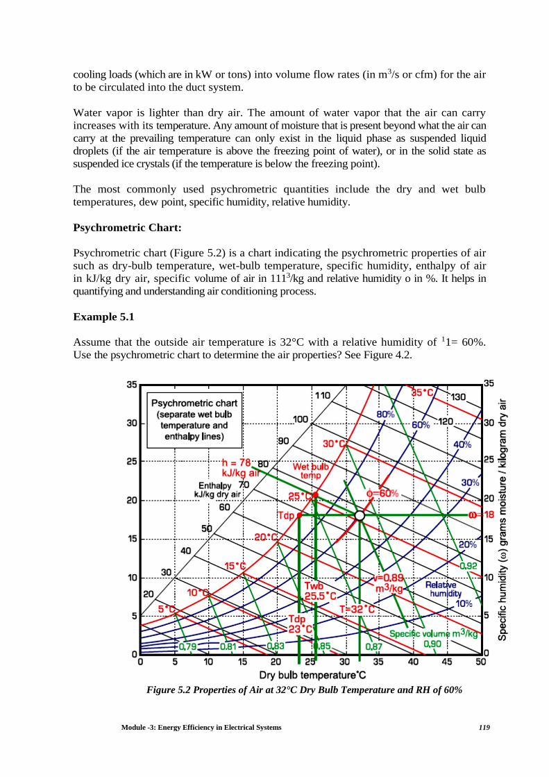
Module -3: Energy Efficiency in Electrical Systems 119
cooling loads (which are in kW or tons) into volume flow rates (in m3/s or cfm) for the air
to be circulated into the duct system.
Water vapor is lighter than dry air. The amount of water vapor that the air can carry
increases with its temperature. Any amount of moisture that is present beyond what the air can
carry at the prevailing temperature can only exist in the liquid phase as suspended liquid
droplets (if the air temperature is above the freezing point of water), or in the solid state as
suspended ice crystals (if the temperature is below the freezing point).
The most commonly used psychrometric quantities include the dry and wet bulb
temperatures, dew point, specific humidity, relative humidity.
Psychrometric Chart:
Psychrometric chart (Figure 5.2) is a chart indicating the psychrometric properties of air
such as dry-bulb temperature, wet-bulb temperature, specific humidity, enthalpy of air
in kJ/kg dry air, specific volume of air in 1113/kg and relative humidity o in %. It helps in
quantifying and understanding air conditioning process.
Example 5.1
Assume that the outside air temperature is 32°C with a relative humidity of 11= 60%.
Use the psychrometric chart to determine the air properties? See Figure 4.2.
Figure 5.2 Properties of Air at 32°C Dry Bulb Temperature and RH of 60%

Module -3: Energy Efficiency in Electrical Systems 120
Solution
Air properties of air at 32°C dry bulb temperature and RH of 60 %
Specific humidity, ὡ = 18 gm-moisture/kg-air
Enthalpy, h = 78 kJ/kg-air
Wet-bulb temperature, Twb = 25.5°C
Dew-point temperature, Tdp = 23°C
The specific volume of the dry air, v = 0.89m3/kg
Comfort Zone
One of the major applications of the Psychrometric Chart is in air conditioning, and we
find that most humans feel comfortable when the temperature is between 22°C and
27°C, and the relative humidity ϕ between 40% and 60%. This defines the "comfort zone"
which is portrayed on the Psychrometric Chart as shown in Figure 4.3. Thus with the aid of the
chart we either heat or cool, add moisture or dehumidify as required in order to bring the air
into the comfort zone.
Example 5.2
Outside air at 35°C and 60% relative humidity is to be conditioned by cooling and re-
heating so as to bring the air to the "comfort zone" with the exit temperature of 24°C
and 53% RH. Using the Psychrometric Chart neatly plot the required air conditioning process
and estimate
(a) the amount of moisture removed, (b) the heat removed, and (c) the amount of heat
added.
See Figure 5.3.

Module -3: Energy Efficiency in Electrical Systems 121
Figure-5.3: Properties of Air
Solution
Using the Figure 5.3
a) The amount of moisture removed = 11.5g-H20 /kg-dry-air
b) The heat removed = (1)-(2), qcool= 48 kJ/kg-dry-air
The amount of heat added = (2)-(3), qheat = 10 kJ/kg-dry-air Air-
Conditioning Systems
Depending on applications, there are several options / combinations, which are available
for use as given below:
Air Conditioning (for comfort / machine)
Split air conditioners
Fan coil units in a larger system
Air handling units in a larger system Refrigeration Systems (for processes)
Small capacity modular units of direct expansion type similar to domestic
refrigerators, small capacity refrigeration units.
Centralized chilled water plants with chilled water as a secondary coolant
for temperature range over 5 °C typically. They can also be used for ice
bank formation.
Brine plants, which use brines as lower temperature, secondary coolant,

Module -3: Energy Efficiency in Electrical Systems 122
for typically subzero temperature applications, which come as modular unit
capacities as well as large centralized plant capacities.
The plant capacities upto 50 TR are usually considered as small capacity,
50 — 250 TR as medium capacity and over 250 TR as large capacity units.
A large industry may have a bank of such units, often with common chilled water
pumps, condenser water pumps, cooling towers, as an off site utility.
The same industry may also have two or three levels of refrigeration & air conditioning
such as:
Comfort air conditioning (20 — 25 °C)
Chilled water system (8 —10 °C)
Brine system (sub-zero applications)
Two principle types of refrigeration plants found in industrial use are: Vapour
Compression Refrigeration (VCR) and Vapour Absorption Refrigeration (VAR). VCR
uses mechanical energy as the driving force for refrigeration, while VAR uses thermal
energy as the driving force for refrigeration.
5.3 Types of Refrigeration System
Vapour Compression Refrigeration
Heat flows naturally from a hot to a colder body. In refrigeration system the opposite
must occur i.e. heat flows from a cold to a hotter body. This is achieved by using a
substance called a refrigerant, which absorbs heat and hence boils or evaporates at a low
pressure to form a gas. This gas is then compressed to a higher pressure, such that it transfers
the heat it has gained to ambient air or water and turns back (condenses) into a liquid. In
this way heat is absorbed, or removed, from a low temperature source and transferred to a
higher temperature source.
The refrigeration cycle can be broken down into the following stages (see Figure 4.4):
1- 2 Low pressure liquid refrigerant in the evaporator absorbs heat from its
surroundings, usually air, water or some other process liquid. During this process it changes
its state from a liquid to a gas, and at the evaporator exit is slightly superheated.
2 - 3 The superheated vapour enters the compressor where its pressure is raised. There
will also be a big increase in temperature, because a proportion of the energy input into the
compression process is transferred to the refrigerant.
3 - 4 The high pressure superheated gas passes from the compressor into the
condenser. The initial part of the cooling process (3 - 3a) desuperheats the gas before it is
then turned back into liquid (3a - 3b). The cooling for this process is usually achieved by
using air or water. A further reduction in temperature happens in the pipe work and liquid
receiver (3b - 4), so that the refrigerant liquid is sub-cooled as it enters the expansion
device.

Module -3: Energy Efficiency in Electrical Systems 123
4 -1 The high-pressure sub-cooled liquid passes through the expansion device, which
both reduces its pressure and controls the flow into the evaporator.
Figure 5.4: Schematic of a Basic Vapour Compression Refrigeration System
It can be seen that the condenser has to be capable of rejecting the combined heat
inputs of the evaporator and the compressor; i.e. (1 - 2) + (2 - 3) has to be the same
as (3 - 4). There is no heat loss or gain through the expansion device.

Module -3: Energy Efficiency in Electrical Systems 124
Alternative Refrigerants for Vapour Compression Systems
The use of CFCs is phased out due to their damaging impact on the protective tropospheric
ozone layer around the earth. The Montreal Protocol of 1987 and the subsequent Copenhagen
agreement of 1992 mandate a reduction in the production of ozone depleting Chlorinated Fluorocarbon
(CFC) refrigerants in a phased manner, with an eventual stop to all production by the year 1996.
As part of the accelerated phase-out of CFCs, India has completely phased out CFCs by 1st
August. 2008.
In response, the refrigeration industry has developed two alternative refrigerants; one based
on Hydrochloro Fluorocarbon (HCFC), and another based on Hydro Fluorocarbon (HFC). The
HCFCs have a 2 to 10% ozone depleting potential as compared to CFCs and also, they have an
atmospheric lifetime between 2 to 25 years as compared to 100 or more years for CFCs (Brandt, 1992).
However, even HCFCs are mandated to be phased out, and only the chlorine free (zero ozone
depletion) HFCs would be acceptable.
The 19th MOP (Meeting of Parties) took a decision to accelerate the phase-out of HCFC
production and consumption for developed and developing countries. The new phase-out schedule
for Article 5 parties as per the decision taken at the 19th MOP is as follows:
Base-level for production & consumption: the average of 2009 and 2010
Freeze= 2013 at the base-level
10% reduction in 2015
35% reduction in 2020
67.5% reduction in 2025
100% reduction in 2030 with a service tail of 2.5% annual average during the period 2030-
2040(Source: Ministry of Environment and Forest, Ozone Cell)
Until now, only one HFC based refrigerant, HFC 134a, has been developed. HCFCs are
comparatively simpler to produce and the three refrigerants 22, 123, and 124 have been
developed. The use of HFCs and HCFCs results in slightly lower efficiencies as compared to
CFCs, but this may change with increasing efforts being made to replace CFCs.
Absorption Refrigeration
The absorption chiller is a machine, which produces chilled water by using heat such as
steam, hot water, gas, oil etc. Chilled water is produced by the principle that liquid
(refrigerant), which evaporates at low temperature, absorbs heat from surrounding when it
evaporates. Pure water is used as refrigerant and lithium bromide solution is used as absorbent
Heat for the vapour absorption refrigeration system can be provided by waste heat extracted
from process, diesel generator sets etc. Absorption systems require electricity to run
pumps only. Depending on the temperature required and the power cost, it may even be
economical to generate heat / steam to operate the absorption system.
Description of the absorption refrigeration concept is given below:

Module -3: Energy Efficiency in Electrical Systems 125
The refrigerant (water) evaporates at
around 4 °C under the high vacuum condition of
754 mmHg in the evaporator. When the
refrigerant (water) evaporates, the latent heat of
vaporization takes the heat from incoming
chilled water.
This latent heat of vaporization can cool the
chilled water which runs into the heat exchanger
tubes in the evaporator by transfer of heat to the
refrigerant (water).
EVAPORATOR
In order to keep evaporating, the refrigerant
vapor must be discharged from the evaporator
and refrigerant (water) must be supplied. The
refrigerant vapor is absorbed into lithium
bromide solution which is convenient to absorb
the refrigerant vapor in the absorber. The heat
generated in the absorption process is led out of
system by cooling water continually. The
absorption also maintains the vacuum inside the
evaporator.
ABSORBER
As lithium bromide solution is diluted, the effect
to absorb the refrigerant vapor reduces. In order
to keep absorption process, the diluted lithium
bromide solution must be made concentrated
lithium bromide.
Absorption chiller is provided with the solution
concentrating system by the heating media such
as steam, hot water, gas, oil, which performs
such function is called generator.
The concentrated solution flows into the absorber
and absorbs the refrigerant vapor again.
HIGH PRESSURE GENERATOR
In order to carryout above works continually and
to make complete cycle, the following two
functions are required.
1. To concentrate and liquefy the evaporated
refrigerant vapor, which is generated in the high
pressure generator.
2. To supply the condensed water to the
evaporator as refrigerant (water).
For these function, condenser is installed.
CONDENSER
A typical schematic of the absorption refrigeration system is given in the Figure 5.5.
Li-Br-water absorption refrigeration systems have a Coefficient of Performance (COP)
in the range of 0.65 - 0.70 and can provide chilled water at 6.7 °C with a cooling water

Module -3: Energy Efficiency in Electrical Systems 126
temperature of 30 °C. Systems capable of providing chilled water at 3 °C are also
available. Ammonia based systems operate at above atmospheric pressures and are capable
of low temperature operation (below 0°C). Absorption machines of capacities in the range of
10-1500 tons are available. Although the initial cost of absorption system is higher than
compression system, operational cost is much lower-if waste heat is used.
Figure 5.5: Schematic of Absorption Refrigeration System
Evaporative Cooling
There are occasions where air conditioning, which stipulates control of humidity up to
50 % for human comfort or for process, can be replaced by a much cheaper and less energy
intensive evaporative cooling.
The concept is very simple and is the same as that used in a cooling tower. Air is
brought in close contact with water to cool it to a temperature close to the wet bulb
temperature. The cool air can be used for comfort or process cooling. The disadvantage
is that the air is rich in moisture. Nevertheless, it is an extremely efficient means of
cooling at very low cost. Large commercial systems employ cellulose filled pads over
which water is sprayed. The temperature can be controlled by controlling the airflow and the
water circulation rate. The possibility of evaporative cooling is especially attractive for comfort
cooling in dry regions. This principle is practiced in textile industries for certain processes.
5.4 Common Refrigerants and Properties
A variety of refrigerants are used in vapor compression systems. The choice of fluid is
determined largely by the cooling temperature required. Commonly used refrigerants are
in the family of chlorinated fluorocarbons (CFCs, also called Freons): R-11, R-12, R-21, R-22

Module -3: Energy Efficiency in Electrical Systems 127
and R-502. The properties of these refrigerants are summarized in Table 4.1 and the
performance of these refrigerants is given in Table 4.2.
Table 5.1 Properties of Commonly used Refrigerants
Refrigerant
Boiling
Point
** (°C)
Freezing
Point
(°C)
Vapor
Pressure
* (kPa)
Vapor
Volume *
(m3 / kg)
Enthalpy *
Liquid
(kJ / kg)
Vapor
(kJ / kg)
R - 11 -23.82 -111.0 25.73 0.61170 191.40 385.43
R - 12 -29.79 -158.0 219.28 0.07702 190.72 347.96
R - 22 -40.76 -160.0 354.74 0.06513 188.55 400.83
R - 502 -45.40 --- 414.30 0.04234 188.87 342.31
R - 7
(Ammonia) -33.30 -77.7 289.93 0.41949 808.71 487.76
* At -10 °C ** At Standard Atmospheric Pressure (101.325 kPa)
Table 5.2 Performance of Commonly used Refrigerants*
Refrigerant Evaporating
Press (kPa)
Condensing
Press (kPa)
Pressure
Ratio
Vapor
Enthalpy
(kJ / kg)
COP**cam
R - 11 20.4 125.5 6.15 155.4 5.03
R - 12 182.7 744.6 4.08 116.3 4.70
R - 22 295.8 1192.1 4.03 162.8 4.66
R - 502 349.6 1308.6 3.74 106.2 4.37
R - 717 236.5 1166.5 4.93 103.4 4.78
* At -15 °C Evaporator Temperature, and 30 °C Condenser Temperature
** COPcarnot = Coefficient of Performance = Temp.Evap. / (Temp.Cond -TeMPEvap)
The choice of refrigerant and the required cooling temperature and load determine the choice
of compressor, as well as the design of the condenser, evaporator, and other auxiliaries.
Additional factors such as ease of maintenance, physical space requirements and availability
of utilities for auxiliaries (water, power, etc.) also influence component selection.
5.5 Compressor Types and Application
For industrial use, open type systems (compressor and motor as separate units) are
normally used, though hermetic systems (motor and compressor in a sealed unit) also find service
in some low capacity applications. Hermetic systems are used in refrigerators, air
conditioners, and other low capacity applications. Industrial applications largely employ
reciprocating, centrifugal and, more recently, screw compressors, and scroll compressors. Water-
cooled systems are more efficient than air-cooled alternatives because the temperatures produced
by refrigerant condensation are lower with water than with air.
Centrifugal Compressors
Centrifugal compressors are the most efficient type (see Figure 4.6) when they are
operating near full load. Their efficiency advantage is greatest in large sizes, and they

Module -3: Energy Efficiency in Electrical Systems 128
offer considerable economy of scale, so they dominate the market for large chillers.
They are able to use a wide range of refrigerants efficiently, so they will probably
continue to be the dominant type in large sizes.
Centrifugal compressors have a single major moving part – an impeller that compresses
the refrigerant gas by centrifugal force. The gas is given kinetic energy as it flows
through the impeller. This kinetic energy is not useful in itself, so it must be converted
to pressure energy. This is done by allowing the gas to slow down smoothly in a
stationary diffuser surrounding the impeller.
Figure 5.6 Centrifugal Compressor
To minimize efficiency loss at reduced loads, centrifugal compressors typically throttle
output with inlet guide vanes located at the inlet to the impeller(s). This method is efficient
down to about 50% load, but the efficiency of this method decreases rapidly below 50% load.
Older centrifugal machines are not able to reduce load much below 50%. This is because of
"surge" in the impeller. As the flow through the impeller is choked off, the gas does not
acquire enough energy to overcome the discharge pressure. Flow drops abruptly at this
point, and an oscillation begins as the gas flutters back and forth in the impeller. Efficiency
drops abruptly, and the resulting vibration can damage the machine. Many older centrifugal
machines deal with low loads by creating a false load on the system, such as by using hot
gas bypass. This wastes the portion of the cooling output that is not required.
Another approach is to use variable-speed drives in combination with inlet guide vanes.
This may allow the compressor to throttle down to about 20% of full load, or less,
without false loading. Changing the impeller speed causes a departure from optimum
performance, so efficiency still declines badly at low loads. A compressor that uses a variable-
speed drive reduces its output in the range between full load and approximately half load by
slowing the impeller speed. At lower loads, the impeller cannot be slowed further, because
the discharge pressure would become too low to condense the refrigerant. Below the minimum
load provided by the variable-speed drive, inlet guide vanes are used to provide further
capacity reduction.

Module -3: Energy Efficiency in Electrical Systems 129
Reciprocating Compressors
The maximum efficiency of reciprocating compressors (see Figure 4.7) is lower than that of
centrifugal and screw compressors. Efficiency is reduced by clearance volume (the
compressed gas volume that is left at the top of the piston stroke), throttling losses at the
intake and discharge valves, abrupt changes in gas flow, and friction. Lower efficiency also
results from the smaller sizes of reciprocating units, because motor losses and friction account
for a larger fraction of energy input in smaller systems.
Figure 5.7: Reciprocating Compressor
Reciprocating compressors suffer less efficiency loss at partial loads than other types,
and they may actually have a higher absolute efficiency at low loads than the other types.
Smaller reciprocating compressors control output by turning on and off. This eliminates all
part-load losses, except for a short period of inefficient operation when the machine starts.
Larger multi-cylinder reciprocating compressors commonly reduce output by disabling
("unloading") individual cylinders. When the load falls to the point that even one cylinder
provides too much capacity, the machine turns off several methods of cylinder unloading
are used, and they differ in efficiency. The most common is holding open the intake valves
of the unloaded cylinders. This eliminates most of the work of compression, but a small
amount of power is still wasted in pumping refrigerant gas to-and-fro through the unloaded
cylinders. Another method is blocking gas flow to the unloaded cylinders, which is called
"suction cutoff"
Variable-speed drives can be used with reciprocating compressors, eliminating the
complications of cylinder unloading. This method is gaining popularity with the drastic
reduction in costs of variable speed drives.
Screw compressors
Screw compressors, sometimes called "helical rotary" compressors, compress refrigerant
by trapping it in the "threads" of a rotating screw-shaped rotor (see Figure 4.8). Screw
compressors have increasingly taken over from reciprocating compressors of medium sizes and
large sizes, and they have even entered the size domain of centrifugal machines. Screw
compressors are applicable to refrigerants that have higher condensing pressures, such as
HCFC-22 and ammonia. They are especially compact. A variety of methods are used to
control the output of screw compressors. There are major efficiency differences among the

Module -3: Energy Efficiency in Electrical Systems 130
different methods. The most common is a slide valve that forms a portion of the housing that
surrounds the screws.
Using a variable-speed drive is another method of capacity control. It is limited to oil-
injected compressors, because slowing the speed of a dry compressor would allow
excessive internal leakage. There are other methods of reducing capacity, such as suction
throttling that are inherently less efficient than the previous two.
Scroll Compressors
The scroll compressor is an old invention that has finally come to the market. The gas is
compressed between two scroll-shaped vanes. One of the vanes is fixed, and the other moves
within it. The moving vane does not rotate, but its center revolves with respect to the center of
the fixed vane, as shown in Figure 4.9. This motion squeezes the refrigerant gas along a
spiral path, from the outside of the vanes toward the center, where the discharge port is located.
The compressor has only two moving parts, the moving vane and a shaft with an off-center
crank to drive the moving vane. Scroll compressors have only recently become practical,
because close machining tolerances are needed to prevent leakage between the vanes, and
between the vanes and the casing.
The features of various refrigeration compressors and application criteria are given in the
Table 5.3.
Table 5.3: Comparison of Different Types of Refrigeration Plants

Module -3: Energy Efficiency in Electrical Systems 131
5.6 Selection of a Suitable Refrigeration System
A clear understanding of the cooling load to be met is the first and most important part
of designing / selecting the components of a refrigeration system. Important factors to be
considered in quantifying the load are the actual cooling need, heat (cool) leaks, and internal heat
sources (from all heat generating equipment). Consideration should also be given to process
changes and / or changes in ambient conditions that might affect the load in the future.
Reducing the load, e.g. through better insulation, maintaining as high a cooling temperature as
practical, etc. is the first step toward minimizing electrical power required to meet refrigeration
needs. With a quantitative understanding of the required temperatures and the maximum,
minimum, and average expected cooling demands, selection of appropriate refrigeration
system (single-stage / multi-stage, economized compression, compound / cascade operation,
direct cooling / secondary coolants) and equipment (type of refrigerant, compressor, evaporator,
condenser, etc.) can be undertaken.

Module -3: Energy Efficiency in Electrical Systems 132
5.7 Performance Assessment of Refrigeration Plants
The cooling effect produced is quantified as tons of refrigeration (TR).
1 TR of refrigeration = 3024 kcal/hr heat rejected. The refrigeration TR is assessed as
TR = Q Cp (Ti — To) / 3024
Where,
Q is mass flow rate of coolant in kg/hr
CP is coolant specific heat in kcal /kg oC
Ti is inlet, temperature of coolant to evaporator (chiller) in °C
To is outlet temperature of coolant from evaporator (chiller) in °C The above TR is also
called as chiller tonnage.
The specific power consumption kW/TR is a useful indicator of the performance of
refrigeration system. By measuring refrigeration duty performed in TR and the kilowatt
inputs, kW/TR is used as a reference energy performance indicator.
In a centralized chilled water system, apart from the compressor unit, power is also
consumed by the chilled water (secondary) coolant pump as well condenser water (for
heat rejection to cooling tower) pump and cooling tower fan in the cooling tower.
Effectively, the overall energy consumption would be towards:
Compressor kW
Chilled water pump kW
Condenser water pump kW
Cooling tower fan kW, for induced / forced draft towers
The specific power consumption for certain TR output would therefore have to include:
Compressor kW/TR
Chilled water pump kW/TR
Condenser water pump kW/TR
Cooling tower fan kW/TR
The overall kW/TR is the sum of the above.
The theoretical Coefficient of Performance (Carnot), COPcarnot - a standard measure of
refrigeration efficiency of an ideal refrigeration system- depends on two key system
temperatures, namely, evaporator temperature Te and condenser temperature T with COP
being given as:
COPcarnot = Te / (Tc - Te)
This expression also indicates that higher COPcarnot is achieved with higher evaporator
temperature and lower condenser temperature.
But COPcarnot is only a ratio of temperatures, and hence does not take into account the
type of compressor. Hence the COP normally used in the industry is given by

Module -3: Energy Efficiency in Electrical Systems 133
Where the cooling effect is the difference in enthalpy across the evaporator and
expressed as kW. The effect of evaporating and condensing temperatures are given in the
Figure 5.8 and Figure 5.9 below:
Figure 5.8 & 5.9 Effect of Evaporator and Temperature on Chiller COP
In the field performance assessment, accurate instruments for inlet and outlet chilled
water temperature and condenser water temperature measurement are required, preferably
with a least count of 0.1°C. Flow measurements of chilled water can be made by an ultrasonic
flow meter directly or inferred from pump duty parameters. Adequacy check of chilled water is
needed often and most units are designed for a typical 0.68 m3/hr per TR (3 gpm/TR) chilled
water flow. Condenser water flow measurement can also be made by a non-contact flow meter
directly or inferred from pump duty parameters. Adequacy check of condenser water is also
needed often, and most units are designed for a typical 0.91 m3/hr per TR (4 gpm / TR)
condenser water flow.
In case of air conditioning units, the airflow at the Fan Coil Units (FCU) or the Air
Handling Units (AHU) can be measured with an anemometer. Dry bulb and wet bulb
temperatures are measured at the inlet and outlet of AHU or the FCU and the refrigeration
load in TR is assessed as;
Where,
Q is the air flow in m3/h
ρ is density of air kg/m3
hin is enthalpy of inlet air kcal/kg

Module -3: Energy Efficiency in Electrical Systems 134
hout is enthalpy of outlet air kcal/kg
Use of psychrometric charts can help to calculate hin and hour from dry bulb, wet bulb
temperature values which are, in-turn measured, during trials, by a whirling psychrometer.
Power measurements at, compressor, pumps, AHU fans, cooling tower fans can be
accomplished by a portable load analyzer.
Estimation of air conditioning load is also possible by calculating various heat loads,
sensible and latent based on inlet and outlet air parameters, air ingress factors, air flow, no. of
people and type of materials stored.
An indicative TR load profile for air conditioning is presented as follows:
Small office cabins = 0.1 TR /m2
Medium size office i.e., 10-30 people occupancy with central AC= 0.06 TR/ m2
Large multistoried office complexes with central AC= 0.04 TR/ m2
Integrated Part Load Value (IPLV)
Although the kW/ TR can serve as an initial reference, it should not be taken as an
absolute since this value is derived from 100% of the equipment's capacity level and is
based on design conditions that are considered the most critical. These conditions occur may
be, for example, during only 1% of the total time the equipment is in operation throughout the
year. Consequently, it is essential to have data that reflects how the equipment operates with
partial loads or in conditions that demand less than 100% of its capacity. To overcome this, an
average of kW/TR with partial loads i.e., Integrated Part Load Value (IPLV) have to be
formulated.
The IPLV is the most appropriate reference, although not considered the best, because it
only captures four points within the operational cycle: 100%, 75%, 50% and 25%.
Furthermore, it assigns the same weight to each value, and most equipment usually operates
at between 50 % and 75% of its capacity. This is why it is so important to prepare specific
analysis for each case that addresses the four points already mentioned, as well as developing
a profile of the heat exchanger's operations during the year.
5.8 Factors Affecting Performance & Energy Efficiency of Refrigeration Plants
Design of Process Heat Exchangers
There is a tendency of the process group to operate with high safety margins which influences
the compressor suction pressure / evaporator set point. For instance, a process cooling
requirement of 15°C would need chilled water at a lower temperature, but the range can
vary from 6°C to say 10°C. At 10°C chilled water temperature, the refrigerant side temperature
has to be lower, say —5°C to +5°C. The refrigerant temperature, again sets the corresponding
suction pressure of refrigerant which decides the inlet duty conditions for work of
compression of the refrigerant compressor. Having the optimum / minimum driving force
(temperature difference) can, thus, help to achieve highest possible suction pressure at the
compressor, thereby leading to less energy requirement. This requires proper sizing of heat
transfer areas of process heat exchangers and evaporators as well as rationalizing the temperature

Module -3: Energy Efficiency in Electrical Systems 135
requirement to highest possible value. A 1°C raise in evaporator temperature can help to
save almost 3 % on power consumption. The TR capacity of the same machine will also increase
with the evaporator temperature, as given in Table 5.4.
Table 5.4 Effect of Variation in Evaporator Temperature on Compressor Power
Consumption
Towards rationalizing the heat transfer areas, the heat transfer coefficient on refrigerant
side can be considered to range from 1400 - 2800 watts /m2K.
The refrigerant side heat transfer areas provided are of the order of 0.5 Sq.m /TR and
above in evaporators.
Condensers in a refrigeration plant are critical equipment that influences the TR
capacity and power consumption demands. Given a refrigerant, the condensing temperature and
corresponding condenser pressure, depend upon the heat transfer area provided,
effectiveness of heat exchange and the type of cooling chosen. A lower condensing
temperature, pressure, in best of combinations would mean that the compressor has to work
between a lower pressure differential as the discharge pressure is fixed by design and
performance of the condenser. The choices of condensers in practice range from air cooled,
air cooled with water spray, and heat exchanger cooled. Generously sized shell and tube
heat exchangers as condensers, with good cooling tower operations help to operate with low
discharge pressure values and the TR capacity of the refrigeration plant also improves. With
same refrigerant, R22, a discharge pressure of 15 kg/cm2 with water cooled shell and tube
condenser and 20 kg/cm2 with air cooled condenser indicate the kind of additional work of
compression duty and almost 30 % additional energy consumption required by the plant.
One of the best option at design stage would be to select generously sized (0.65 m2/TR and
above) shell and tube condensers with water-cooling as against cheaper alternatives like
air cooled condensers or water spray atmospheric condenser units.
The effect of condenser temperature on refrigeration plant energy requirements is given
in Table 5.5.

Module -3: Energy Efficiency in Electrical Systems 136
Table 5.5 Effect of Variation in Condenser Temperature on Compressor Power
Maintenance of Heat Exchanger Surfaces
After ensuring procurement, effective maintenance holds the key to optimizing power
consumption.
Heat transfer can also be improved by ensuring proper separation of the lubricating oil
and the refrigerant, timely defrosting of coils, and increasing the velocity of the
secondary coolant (air, water, etc.). However, increased velocity results in larger
pressure drops in the distribution system and higher power consumption in pumps / fans.
Therefore, careful analysis is required to determine the most effective and efficient
option.
Fouled condenser tubes force the compressor to work harder to attain the desired
capacity. For example, a 0.8 mm scale build-up on condenser tubes can increase energy
consumption by as much as 35 %. Similarly, fouled evaporators (due to residual
lubricating oil or infiltration of air) result in increased power consumption. Equally
important is proper selection, sizing, and maintenance of cooling towers. A reduction of
0.55°C temperature in water returning from the cooling tower reduces compressor
power consumption by 3.0 % (see Table 4.6).
Table 5.6 Effect of Poor Maintenance on Compressor Power Consumption
* 15 ton reciprocating compressor based system. The power consumption is lower than
that for systems typically available in Bangladesh. However, the percentage change in
power consumption is indicative of the effect of poor maintenance.
Multi-Staging for Efficiency
Efficient compressor operation requires that the compression ratio be kept low, to
reduce discharge pressure and temperature. For low temperature applications involving
high compression ratios, and for wide temperature requirements, it is preferable (due to

Module -3: Energy Efficiency in Electrical Systems 137
equipment design limitations) and often economical to employ multi-stage reciprocating
machines or centrifugal / screw compressors.
Multi-staging systems are of two-types: compound and cascade — and are applicable to
all types of compressors. With reciprocating or rotary compressors, two-stage compressors are
preferable for load temperatures from -20 to -58°C, and with centrifugal machines for
temperatures around -3°C.
In multi-stage operation, a first-stage compressor, sized to meet the cooling load, feeds
into the suction of a second-stage compressor after inter-cooling of the gas. Apart of the high-
pressure liquid from the condenser is flashed and used for liquid sub-cooling. The second
compressor, therefore, has to meet the load of the evaporator and the flash gas. A single
refrigerant is used in the system, and the work of compression is shared equally by the two
compressors. Therefore, two compressors with low compression ratios can in combination
provide a high compression ratio.
For temperatures in the range of -46°C to -101°C, cascaded systems are preferable. In this
system, two separate systems using different refrigerants are connected such that one
provides the means of heat rejection to the other. The chief advantage of this system is
that a low temperature refrigerant which has a high suction temperature and low specific
volume can be selected for the low-stage to meet very low temperature requirements.
Matching Capacity to System Load
During part-load operation, the evaporator temperature rises and the condenser temperature
falls, effectively increasing the COP. But at the same time, deviation from the design
operation point and the fact that mechanical losses form a greater proportion of the total power
negate the effect of improved COP, resulting in lower part-load efficiency.
Therefore, consideration of part-load operation is important, because most refrigeration
applications have varying loads. The load may vary due to variations in temperature and
process cooling needs. Matching refrigeration capacity to the load is a difficult exercise, requiring
knowledge of compressor performance, and variations in ambient conditions, and detailed
knowledge of the cooling load.
Capacity Control and Energy Efficiency
The capacity of compressors is controlled in a number of ways. Capacity control of
reciprocating compressors through cylinder unloading results in incremental (step-by-
step) modulation as against continuous capacity modulation of centrifugal through vane
control and screw compressors through sliding valves. Therefore, temperature control requires
careful system design. Usually, when using reciprocating compressors in applications with
widely varying loads, it is desirable to control the compressor by monitoring the return
water (or other secondary coolant) temperature rather than the temperature of the water
leaving the chiller. This prevents excessive on-off cycling or unnecessary loading / unloading
of the compressor. However, if load fluctuations are not high, the temperature of the water
leaving the chiller should be monitored. This has the advantage of preventing operation at
very low water temperatures, especially when flow reduces at low loads. The leaving water
temperature should be monitored for centrifugal and screw chillers.

Module -3: Energy Efficiency in Electrical Systems 138
Capacity regulation through speed control is the most efficient option. However, when
employing speed control for reciprocating compressors, it should be ensured that the
lubrication system is not affected. In the case of centrifugal compressors, it is usually
desirable to restrict speed control to about 50 % of the capacity to prevent surging. Below 50
%, vane control or hot gas bypass can be used for capacity modulation.
The efficiency of screw compressors operating at part load is generally higher than
either centrifugal compressors or reciprocating compressors, which may make them
attractive in situations where part-load operation is common. Screw compressor performance
can be optimized by changing the volume ratio. In some cases, this may result in higher
full-load efficiencies as compared to reciprocating and centrifugal compressors. Also, the
ability of screw compressors to tolerate oil and liquid refrigerant slugs makes them preferred
in some situations.
Multi-level Refrigeration for Plant Needs
The selection of refrigeration systems also depends on the range of temperatures
required in the plant. For diverse applications requiring a wide range of temperatures, it is
generally more economical to provide several packaged units (several units distributed
throughout the plant) instead of one large central plant. Another advantage would be the
flexibility and reliability accorded. The selection of packaged units could also be made
depending on the distance at which cooling loads need to be met. Packaged units at load centers
reduce distribution losses in the system. Despite the advantages of packaged units, central
plants generally have lower power consumption since at reduced loads power consumption can
reduce significantly due to the large condenser and evaporator surfaces.
Many industries use a bank of compressors at a central location to meet the load.
Usually the chillers feed into a common header from which branch lines are taken to
different locations in the plant. In such situations, operation at part-load requires extreme
care. For efficient operation, the cooling load, and the load on each chiller must be
monitored closely. It is more efficient to operate a single chiller at full load than to operate
two chillers at part-load. The distribution system should be designed such that
individual chillers can feed all branch lines. Isolation valves must be provided to
ensure that chilled water (or other coolant) does not flow through chillers not
in operation. Valves should also be provided on branch lines to isolate sections where
cooling is not required. This reduces pressure drops in the system and reduces power
consumption in the pumping system. Individual compressors should be loaded to their full
capacity before operating the second compressor. In some cases it is economical to provide a
separate smaller capacity chiller, which can be operated on an on-off control to meet peak
demands, with larger chillers meeting the base load.
Flow control is also commonly used to meet varying demands. In such cases the savings
in pumping at reduced flow should be weighed against the reduced heat transfer in coils
due to reduced velocity. In some cases, operation at normal flow rates, with subsequent longer
periods of no-load (or shut-off) operation of the compressor, may result in larger savings.
Chilled Water Storage
Depending on the nature of the load, it is economical to provide a chilled water storage
facility with very good cold insulation. Also, the storage facility can be fully filled to

Module -3: Energy Efficiency in Electrical Systems 139
meet the process requirements so that chillers need not be operated continuously. This system
is usually economical if small variations in temperature are acceptable. This system has the
added advantage of allowing the chillers to be operated at periods of low electricity
demand to reduce peak demand charges - Low tariffs offered by some electric utilities for
operation at night time can also be taken advantage of by using a storage facility. An added
benefit is that lower ambient temperature at night lowers condenser temperature and thereby
increases the COP.
If temperature variations cannot be tolerated, it may not be economical to provide a
storage facility since the secondary coolant would have to be stored at a temperature
much lower than required to provide for heat gain. The additional cost of cooling to a
lower temperature may offset the benefits. The solutions are case specific. For example, in
some cases it may be possible to employ large heat exchangers, at a lower cost burden than
low temperature chiller operation, to take advantage of the storage facility even when
temperature variations are not acceptable. Ice bank systems which store ice rather than
water are often economical.
System Design Features
In overall plant design, adoption of good practices improves the energy efficiency
significantly. Some areas for consideration are:
Design of cooling towers with FRP impellers and film fills, PVC drift
eliminators, etc.
Use of softened water for condensers in place of raw water.
Use of economic insulation thickness on cold lines, heat exchangers, considering
cost of heat gains and adopting practices like infrared thermography for monitoring -
applicable especially in large chemical / fertilizer / process industry.
Adoption of roof coatings / cooling systems, false ceilings / as applicable, to
minimize refrigeration load.
Adoption of energy efficient heat recovery devices like air to air heat exchangers
to pre-cool the fresh air by indirect heat exchange; control of relative humidity
through indirect heat exchange rather than use of duct heaters after chilling.
Adopting of variable air volume systems; adopting of sun film application for heat
reflection; optimizing lighting loads in the air conditioned areas; optimizing
number of air changes in the air conditioned areas are few other examples.
5.9 Performance Assessment of window, split and package air conditioning units
Air Conditioners
Energy Efficiency Ratio (EER): EER is calculated by dividing a chiller's cooling
capacity (in watts) by its power input (in watts) at full-load conditions. This definition
of EER has been adopted in BEE star labeling programme.
The energy efficiency ratio (EER) = Refrigeration effect in Watts/ Power input in Watts
Based on the condition of the air, the air properties such as specific volume and enthalpy
at both inlet and out let conditions can be obtained from psychrometric charts. From these
parameters the capacity delivered by the air conditioner can be evaluated, which when
compared with power drawn would reveal its performance in terms of kW/TR and EER.

Module -3: Energy Efficiency in Electrical Systems 140
Performance Assessment of Package Air Conditioner -
Example 5.5
Package air conditioner
capacity
- 10 TR
Average Air Velocity - 2.27 m/s (across suction side
filter)
Cross Sectional Area - 0.58 m2
Air Flow Rate - 1.32 m3/sec - 4751 m3/hr
Inlet Air Condition
DBT - 20 °C
WBT - 14 °C
Sp.Vol - 0.8405 m3/kg
Enthalpy - 9.37 kcal/kg
Outlet Air Condition
DBT - 12.7 °C
WBT - 11.3 °C
Enthalpy - 7.45 kcal/kg
Cooling Effect Delivered - 3.6 TR = 12.7 kW
Power Drawn
Compressor - 4.71 kW
- 4.3 kW (shaft power@ 90%
motor efficiency)
Pump - 2.14 kW
C.T Fan - 0.384 kW
Specific Energy Consumption
Compressor - 1.31 kW/TR
Overall - 2 kW/TR
EER - 12700/4300
- 2.95 W/W
Note: The Package A/C unit has two compressors of 5 TR capacity each, of which only
one was in operation due to low cooling load.
5.10 Cold Storage Systems
A Refrigerated storage which includes cold storage and frozen food storage is the best
known method of preservation of food to retain its value and flavor.
The refrigeration system in a cold storage is usually a vapour compression system
comprising the compressor, condenser, receiver, air cooling units and associate piping and
controls.

Module -3: Energy Efficiency in Electrical Systems 141
In smaller cold rooms and walk-ins the practice is to use air cooled condensing units with
sealed, semi-sealed or open type compressors. In the light of the CFC phase out the
trend now is to use HCFC22, HFC-134a or other substitute refrigerants. In the medium and
large sized units the practice is to use a central plant with ammonia as the refrigerant.
In some present day medium and large sized units with pre-fabricated (insulated) panel
construction, the trend is to use modular HCFC-22/HFC units which are compact,
lightweight and easy to maintain.
Energy Saving Opportunities in Cold Storage Systems:
Energy cost constitutes a major part of the running cost of a cold store. Apart from the
problems of the availability of electrical energy, the ever increasing rate of electrical energy
seriously affects the economic viability of cold store units.
Following are some of the measures adopted to achieve energy efficient operation.
Cold Store Building Design: Proper orientation, compact arrangement of
chambers, shading of exposed walls, adequate insulation etc. are some of the
important factors.
Refrigeration System: The system must be designed for optimum operating
conditions like evaporating and condensing temperatures, as these conditions have
a direct bearing on energy consumption.
Compressor capacity control system helps in energy savings during partial load
operation.
Control System: The proper control systems for refrigerant level, room
temperature, compressor capacity etc., are required to further optimize energy
consumption.
Air Curtain or Strip Curtain: The use of air curtains and strip curtains is a common
feature in present day cold stores as they help reduce air infiltration due to
frequent and sometimes long door openings. Fan operated air curtains are
expensive and work on electrical power whereas strip curtains are cheaper and
need no energy for operation.
Heat Recovery System: In processing plant cold stores, a heat reclaim system can
be installed to recover a part of the heat rejected by the refrigeration system. This
can be gainfully utilised in generating hot water free of cost.
5.11 Heat Pumps aim (heir Applications
Heat Pump Technology
A heat pump is same as an air conditioner except that the heat rejected in an air conditioner
becomes the useful heat output. Heat flows naturally from a higher to a lower
temperature. Heat pumps, however, are able to force the heat flow in the other direction,
using a relatively small amount of high quality drive energy (electricity, fuel, or high-
temperature waste heat). For the example shown in 4.12 the heat pump takes three units of energy
from atmosphere and with an additional one unit by way of compressor work is able to
provide four units of energy at a higher temperature. Thus heat pumps can transfer heat from
natural heat sources in the surroundings, such as the air, ground or water, or from man-made heat
sources such as industrial or domestic waste, to a building or an industrial application.

Module -3: Energy Efficiency in Electrical Systems 142
Figure 5.10 Heat Pump
In order to transport heat from a heat source to a heat sink, external energy is needed to drive the
heat pump. Theoretically, the total heat delivered by the heat pump is equal to the heat
extracted from the heat source, plus the amount of drive energy supplied. Electrically-
driven heat pumps for heating buildings typically supply 100 kWh of heat with just 20-40
kWh of electricity. Many industrial heat pumps can achieve even higher performance, and
supply the same amount of heat with only 3-10 kWh of electricity. The principle of
operation of heat pump is shown in the Figure 5.11.
Figure 5.11 Principle of Operation

Module -3: Energy Efficiency in Electrical Systems 143
Heat Pump Applications
Industrial heat pumps are mainly used for:
• Space heating
• Heating of process streams
• Water heating for washing, sanitation and cleaning
• Steam production
• Drying/dehumidification
• Evaporation
• Distillation
• Concentration
When heat pumps are used in drying, evaporation and distillation processes, heat is
recycled within the process. For heating of the space, process streams and steam production,
the heat pumps utilise (waste) heat sources between 20°C and 100°C.
5.12 Ventilation Systems
Ventilation can be simply described as air circulation, the extraction of stale, overheated
and contaminated air and supply and distribution of fresh air in amounts necessary to
provide healthy and comfortable conditions for the occupants of the room. The ventilation
effectiveness is dictated by number of Air Changes per Hour (ACH). The number air
changes depend on the purpose and function. Typical air changes are given in Table 5.7
for various operations.
Table 5.7 Typical Air Changes per Hour
Location Air changes per hour
Boiler room 15 — 30
Compressor room 10 — 12
Conference rooms 10 — 20
Engine rooms 15 — 30
Lavatories 6 — 15
Offices 6 —10
Welding shops 15 — 30
Calculation of ventilation rate: If the compressor room size is 15 m (L) X 10 m (B) X
4 m (H) then the ventilation rate is =LxBXHXAC
=15 X10 X 4 X10
= 6000 m3/hr
5.13 Ice Bank Systems
Ice Bank System is a proven technology that has been utilized for decades Thermal
energy storage takes advantage of low cost, off-peak electricity, produced more efficiently
throughout the night, to create and store cooling energy for use when electricity tariffs are
higher, typically during the day. There are full- and partial- load Off-Peak Cooling systems.
The essential element for either full- or partial- storage configurations are thermal- energy
storage tanks. Each tank contains a spiral-wound, polyethylene-tube heat exchanger

Module -3: Energy Efficiency in Electrical Systems 144
surrounded with water. ICEBANK tanks are available in a variety of sizes ranging from
45 to over 500 ton-hours. These systems are economical based on the electricity tariff of
particular utility. These systems can be employed to meet the air conditioning requirements
in the commercial buildings as well as to meet the chilling requirements in Diary and process
industry. The main advantage of these systems is to reduce the peak demand of the utility and
also reduce the cost of operation for the end user.
How Ice Bank Works?
With a partial-storage system, the chiller can be 40 to 50 percent smaller than other
HVAC systems, because the chiller works in conjunction with the ICEBANK tanks
during on-peak daytime hours to manage the building's cooling load. During off-peak night
time hours, the chiller charges the ICEBANK tanks for use during the next day's cooling. The
lowest possible average load is obtained by extending the chiller hours of operation.
5.14 Humidification Systems
This is a process involving reduction in dry bulb temperature and increase in specific
humidity. The atmospheric conditions with respect to humidity play a very important
part in many manufacturing processes. For example in textile processing the properties like
dimensions, weight, tensile strength, elastic recovery, electrical resistance, rigidity etc. of all
textile fibre are influenced by humidity maintained. Temperature does not have a great effect
on the fibres but the temperature dictates the amount of moisture the air will hold in
suspension and, therefore, temperature and humidity must be considered together.
Humidification system without chilling helps to maintain only the RH% without much
difficulty.
Adiabatic saturation or evaporative cooling
In this process (Figure 5.12) air comes in direct contact with water in the air washer.
There is heat and mass transfer between air and water. The humidity ratio of air increases. If
the time of contact is sufficient, the air gets saturated. Latent heat of evaporation required for
conversion of water into water vapor is taken from the remaining water. When equilibrium
conditions are reached, water cools down to the wet bulb temperature of the air. If the air washer
is ideal, the dry bulb temperature and wet bulb temperature of the air would be equal. Dry bulb
temperature of the air goes down in the process and the effect of cooling is due to the
evaporation of some part of the water. That is why it is called Evaporative Cooling.
The sensible heat is decreased as the temperature goes down but the latent heat goes up
as water vapour is added to the air. The latent heat required by the water which is
evaporated in the air is drawn from the sensible heat of the same air. Thus it is
transformation of sensible heat to latent heat. During this process the enthalpy of air remains
the same. If humidity ratios of saturated air and of the air before saturation are known, then
the difference between the two would be the amount of water vapour absorbed by unit weight of
dry air.

Module -3: Energy Efficiency in Electrical Systems 145
Figure 5.12 Air Washer Unit
Humidifying Air by adding Water
If water is added to air without any heat supply the state of air change adiabatic along a
constant enthalpy line in the psychrometric chart. The dry bulb temperature of the air
decreases.
The amount of added water can be expressed as
mw = v ρ (ὡout - win)
Where,
mw = mass of added water (kg/hr)
v = volume flow of air (m3/hr)
ρ = density of air - vary with temperature, 1.293 kg/m3 at 20°C (kg/m3)
ὡ = specific humidity of air (kg/kg)
Example 5.6
Humidifying Air by adding Water
In an air washer of textile humidification system airflow of 3000 m3/h at 25°C and 10%
relative humidity is humidified to 60% relative humidity by adding water through spray
nozzles. Calculate the amount of water required. The specific humidity of air at inlet and
outlet are 0.002 kg/kg and 0.0062 kg/kg respectively.
Solution
The amount of water added can be calculated as:
mw = 3000 X 1.184 X (0.0062 - 0.002) 14.9 kg/h
5.15 Energy Saving Opportunities
a) Cold Insulation
Insulate all cold lines / vessels using economic insulation thickness to minimize heat
gains; and choose appropriate (correct) insulation.

Module -3: Energy Efficiency in Electrical Systems 146
b) Building Envelope
Optimise air conditioning volumes by measures such as use of false ceiling and
segregation of critical areas for air conditioning by air curtains.
c) Building Heat Loads Minimisation
Minimise the air conditioning loads by measures such as roof cooling, roof painting,
efficient lighting, pre-cooling of fresh air by air- to-air heat exchangers, variable volume air
system, otpimal thermo-static setting of temperature of air conditioned spaces, sun film
applications, etc.
d) Process Heat Loads Minimisation
Minimize process heat loads in terms of TR capacity as well as refrigeration level, i.e.,
temperature required, by way of:
Flow optimization
Heat transfer area increase to accept higher temperature coolant
Avoiding wastages like heat gains, loss of chilled water, idle flows.
Frequent cleaning / de-scaling of all heat exchangers
e) At the Refrigeration A/C Plant Area
Ensure regular maintenance of all A/C plant components as per manufacturer
guidelines.
Ensure adequate quantity of chilled water and cooling water flows, avoid bypass
flows by closing valves of idle equipment.
Minimize part load operations by matching loads and plant capacity on line;
adopt variable speed drives for varying process load.
Make efforts to continuously optimize condenser and evaporator parameters for
minimizing specific energy consumption and maximizing capacity.
Adopt VAR system where economics permit as a non-CFC solution.
5.16 Case Study: Screw Compressor Application
Background
Rotary Screw Compressors are widely used for refrigeration applications to compress
ammonia & other refrigerating gases. A typical sectional view of the compressor is
shown below in Figure 5.13.

Module -3: Energy Efficiency in Electrical Systems 147
Figure 5.13 Section of Screw Compressor showing the meshing screws & slide valve
The table 5.10 below gives the measured system data during compressor running at part
load condition.
Table 5.10 Performance parameters for partial load conditions
Volumetric
refrigerant
flow (m3)
Suction
Pressure
(kg/cm2)
Discharge
Pressure
(kg/cm2)
Inlet
Temp.
(°C)
Outlet
Temp.
(°C)
Total
refrigeration
load
(Calories)
Total
refrigeration
load
(TR)
21.03 3.19 11.89 28.08 1.49 558964 184.73
26.62 3.16 11.65 26.85 2.12 658336 217.57
26 3.17 11.63 27.75 1.68 678000 224.07
28 3.22 11.7 27.91 1.92 727650 240.47
32 3.22 11.78 27.98 2.28 822400 271.79
20.13 3.25 12.22 27.28 1.5 518947 171.5
21.71 3.25 12.38 27.77 1.6 568197 187.78
23.36 3.25 12.52 28.4 1.64 625306 206.65
28.15 3.25 11.99 28.58 1.27 714310 236.07
28.51 3.25 12.31 28.7 1.54 774362 255.91
The table 5.11 below gives the power consumption data for partial load operation with
and without VFD.

Module -3: Energy Efficiency in Electrical Systems 148
Table 5.11 Power consumption for partial load operation (with & without VFD)
Power
consumed
without VFD
(kW)
Power
consumed
with VFD
(kW)
Measured Power
consumed per ton
of refrigeration load
without VFD
(kW/TR)
Measured Power
consumed per ton
of refrigeration
load with VFD
(kW/TR)
Hourly savings
due to VFD
operation
(kW)
173.14 127.25 0.94 0.69 45.89
203.93 149.87 0.94 0.69 54.06
210.02 154.35 0.94 0.69 55.67
225.4 165.65 0.94 0.69 59.75
254.75 187.22 0.94 0.69 67.53
160.75 118.14 0.94 0.69 42.61
176 129.35 0.94 0.69 46.65
193.69 142.35 0.94 0.69 51.34
221.26 162.61 0.94 0.69 58.65
239.87 176.28 0.94 0.69 63.59
Average hourly power savings = 57.6 kW
Average yearly energy savings (250 days x 10 hours) = 136435 kWh Average yearly monetary
savings (BDT. 6.00/kWh) = BDT. 8, 18,610 /-
Example 5.7
The measured values of a 20 TR package air conditioning plant are given below:
Average air velocity across suction side filter: 2.5 m/s
Cross Sectional area of suction: 1.2 m2
Inlet air = Dry Bulb: 20°C, Wet Bulb: 14 °C, Enthalpy: 9.37 kcal/kg
Outlet air = Dry Bulb: 12.7 °C, Wet Bulb: 11.3 °C; Enthalpy: 7.45 kcal/kg
Specific volume of air: 0.85 m3/kg
Power drawn: by compressor: 10.69 kW
by Pump: 4.86 kW
by Cooling tower fan: 0.87 kW
Calculate:
a) Air Flow rate in m3/hr
b) Cooling effect delivered in kW
c) Specific power consumption of compressor in kW/TR
d) Overall kW/TR
e) Energy Efficiency Ratio in kW/kW
Solution
Air flow rate = 2.5*1.2 = 3 m3/sec = 10800 m3/hr
Cooling Effect delivered = [(9.37-7.45)*10800]/(0.85*3024)
= 8.07 TR = 28.32 kW
Compressor kW/TR = 10.69/8.07 = 1.32
Overall kW/TR = (10.69+4.86+0.87)/8.07 = 2.04
Energy Efficiency Ratio (EER) in kW/kW = 28.32/10.69 = 2.65

Module -3: Energy Efficiency in Electrical Systems 149
Chapter 6: Pumps And Pumping System
6.1 Pump Types
Pumps come in a variety of sizes for a wide range of applications. They can be
classified according to their basic operating principle as dynamic or displacement pumps.
Dynamic pumps can be sub-classified as centrifugal and special effect pumps. Displacement
pumps can be sub-classified as rotary or reciprocating pumps.
In principle, any liquid can be handled by any of the pump designs. Where different
pump designs could be used, the centrifugal pump is generally the most economical
followed by rotary and reciprocating pumps. Although, positive displacement pumps are
generally more efficient than centrifugal pumps, the benefit of higher efficiency tends to
be offset by increased maintenance costs.
Since, worldwide, centrifugal pumps account for the majority of electricity used by
pumps, the focus of this chapter is on centrifugal pump
Centrifugal Pumps
A centrifugal pump (Figure 6.1) is of a very simple design. The two main parts of the pump
are the impeller and the diffuser. Impeller, which is the only moving part, is attached to a
shaft and driven by a motor. Impellers are generally made of bronze, polycarbonate, cast
iron, stainless steel as well as other materials. The diffuser (also called as volute) houses the
impeller and captures and directs the water off the impeller.
Water enters the center (eye) of the impeller and exits the impeller with the help of centrifugal
force. As water leaves the eye of the impeller a low-pressure area is created, causing more
water to flow into the eye. Atmospheric pressure and centrifugal force cause this to
happen. Velocity is developed as the water flows through the impeller spinning at high
speed. The water velocity is collected by the diffuser and converted to pressure by specially
designed passageways that direct the flow to the discharge of the pump, or to the next impeller
should the pump have a multi-stage configuration.
Figure 6.1 Centrifugal Pump
The pressure (head) that a pump will develop is in direct relationship to the impeller
diameter, the number of impellers, the size of impeller eye, and shaft speed. Capacity is

Module -3: Energy Efficiency in Electrical Systems 150
determined by the exit width of the impeller. The head and capacity are the main factors,
which affect the horsepower size of the motor to be used. The more the quantity of water to be
pumped, the more energy is required.
A centrifugal pump is not positive acting, it will not pump the same volume always. The
greater the depth of the water, the lesser is the flow from the pump. Also, when it pumps
against increasing pressure, the less it will pump. For these reasons it is important to select
a centrifugal pump that is designed to do a particular job.
Since the pump is a dynamic device, it is convenient to consider the pressure in terms of
head i.e. meters of liquid column. The pump generates the same head of liquid whatever
the density of the liquid being pumped. The actual contours of the hydraulic passages of the
impeller and the casing are extremely important, in order to attain the highest efficiency possible.
The standard convention for centrifugal pump is to draw the pump performance curves
showing Flow on the horizontal axis and Head generated on the vertical axis. Efficiency, Power
& NPSH Required (described later), are also all conventionally shown on the vertical axis,
plotted against Flow, as illustrated in Figure 6.2.
Figure 6.2 Pump Performance
Given the significant amount of electricity attributed to pumping systems, even small
improvements in pumping efficiency could yield very significant savings of electricity.
The pump is among the most inefficient of the components that comprise a pumping system,
including the motor, transmission drive, piping and valves.
Hydraulic Power, Pump Shaft Power and Motor Input Power
Hydraulic Power Ph = Q (m3/s) x Total Differential head, hd - hs (m) x p (kg/m3) x g
(m/s2) / 1000
Where hd -discharge head, hs-suction head, ρ-density of the liquid, g- acceleration due to
gravity
Pump Shaft Power Ps = Hydraulic power, Ph / Pump Efficiency, ηPump
Motor Input Power = Pump shaft power Ps / Motor Efficiency, ηMotor
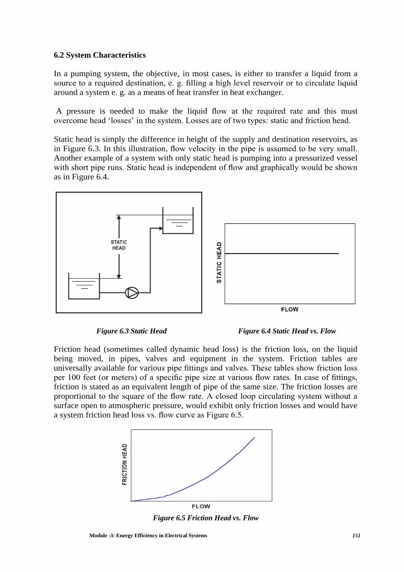
Module -3: Energy Efficiency in Electrical Systems 151
6.2 System Characteristics
In a pumping system, the objective, in most cases, is either to transfer a liquid from a
source to a required destination, e. g. filling a high level reservoir or to circulate liquid
around a system e. g. as a means of heat transfer in heat exchanger.
A pressure is needed to make the liquid flow at the required rate and this must
overcome head ‘losses’ in the system. Losses are of two types: static and friction head.
Static head is simply the difference in height of the supply and destination reservoirs, as
in Figure 6.3. In this illustration, flow velocity in the pipe is assumed to be very small.
Another example of a system with only static head is pumping into a pressurized vessel
with short pipe runs. Static head is independent of flow and graphically would be shown
as in Figure 6.4.
Figure 6.3 Static Head Figure 6.4 Static Head vs. Flow
Friction head (sometimes called dynamic head loss) is the friction loss, on the liquid
being moved, in pipes, valves and equipment in the system. Friction tables are
universally available for various pipe fittings and valves. These tables show friction loss
per 100 feet (or meters) of a specific pipe size at various flow rates. In case of fittings,
friction is stated as an equivalent length of pipe of the same size. The friction losses are
proportional to the square of the flow rate. A closed loop circulating system without a
surface open to atmospheric pressure, would exhibit only friction losses and would have
a system friction head loss vs. flow curve as Figure 6.5.
Figure 6.5 Friction Head vs. Flow

Module -3: Energy Efficiency in Electrical Systems 152
Most systems have a combination of static and friction head and the system curves for
two cases are shown in Figures 6.6 and 6.7. The ratio of static to friction head over the
operating range influences the benefits achievable from variable speed drives which
shall be discussed later
Figure 6.6 System with High Static Head Figure 6.7 System with Low Static Head
Static head is a characteristic of the specific installation and reducing this head where
this is possible generally helps both the cost of the installation and the cost of pumping
the liquid. Friction head losses must be minimized to reduce pumping cost, but after
eliminating unnecessary pipe fittings and length, further reduction in friction head will
require larger diameter pipe, which adds to capital cost.
6.3 Pump Curves
The performance of a pump can be expressed graphically as head against flow rate. The
centrifugal pump has a curve where the head falls gradually with increasing flow. This
is called the pump characteristic curve (Head — Flow curve). See Figure 6.8.
Figure 6.8 Head-Flow Curve

Module -3: Energy Efficiency in Electrical Systems 153
Pump operating point
When a pump is installed in a system the effect can be illustrated graphically by
superimposing pump and system curves. The operating point will always be where the
two curves intersect. Figure: 6.9.
Figure 6.9 Pump Operating Point
If the actual system curve is different in reality to that calculated, the pump will operate
at a flow and head different to that expected. For a centrifugal pump, an increasing
system resistance will reduce the flow, eventually to zero, but the maximum head is
limited as shown. Even so, this condition is only acceptable for a short period without
causing problems. An error in the system curve calculation is also likely to lead to a
centrifugal pump selection, which is less than optimal for the actual system head losses.
Adding safety margins to the calculated system curve to ensure that a sufficiently large
pump is selected will generally result in installing an oversized pump, which will
operate at an excessive flow rate or in a throttled condition, which increases energy
usage and reduces pump life.
6.4 Factors Affecting Pump Performance
Matching Pump and System Head-flow Characteristics
Centrifugal pumps are characterized by the relationship between the flow rate (Q) they
produce and the pressure (H) at which the flow is delivered. Pump efficiency varies with
flow and pressure, and it is highest at one particular flow rate.
The Figure 6.10 below shows a typical vendor-supplied head-flow curve for a
centrifugal pump. Pump head-flow curves are typically given for clear water. The choice
of pump for a given application depends largely on how the pump head-flow
characteristics match the requirement of the system downstream of the pump.

Module -3: Energy Efficiency in Electrical Systems 154
Figure 6.10 Typical Centrifugal Pump Performance Curve
Effect of over sizing the pump
As mentioned earlier, pressure losses to be overcome by the pumps are functions of flow
-the system characteristics are also quantified in the form of head-flow curves. The
system curve is basically a plot of system resistance i.e. head to be overcome by the
pump versus various flow rates. The system curves change with the physical
configuration of the system; for example, the system curves depends upon height or
elevation, diameter and length of piping, number and type of fittings and pressure drops
across various equipment - say a heat exchanger.
A pump is selected based on how well the pump curve and system head-flow curves
match. The pump operating point is identified as the point, where the system curve
crosses the pump curve when they are superimposed on each other. The Figure 6.11
shows the effect on system curve with throttling.
In the system under consideration, water has to be first lifted to a height-this represents
the static head.
Then, we make a system curve, considering the friction and pressure drops in the
system-this is shown as the green curve.
Suppose, we have estimated our operating conditions as 500 m3/hr flow and 50 m head,
we will chose a pump curve which intersects the system curve (Point A) at the pump’s
best efficiency point (BEP).

Module -3: Energy Efficiency in Electrical Systems 155
Figure 6.11 Effect on System Curve with Throttling
But, in actual operation, we find that 300 m3/hr is sufficient. The reduction in flow rate
has to be effected by a throttle valve. In other words, we are introducing an artificial
resistance in the system.
Due to this additional resistance, the frictional part of the system curve increases and
thus the new system curve will shift to the left - this is shown as the red curve.
So the pump has to overcome additional pressure in order to deliver the reduced flow.
Now, the new system curve will intersect the pump curve at point B. The revised
parameters are 300 m3/hr at 70 m head. The red double arrow line shows the additional
pressure drop due to throttling.
It may be noted that the best efficiency point has shifted from 82% to 77% efficiency.
So it is actually needed to operate at point C, which is 300 m3/hr on the original system
curve. The head required at this point is only 42 meters.
Hence a new pump is needed, which will operate with its best efficiency point at C. But
there are other simpler options rather than replacing the pump. The speed of the pump
can be reduced or the existing impeller can be trimmed (or new lower size impeller).
The blue pump curve represents either of these options.
Energy loss in throttling
Consider a case (see Figure 6.12) where we need to pump 68 m3/hr of water at 47 m
head. The pump characteristic curves (A. . .E) for a range of pumps are given in the
Figure 6.12.
If we select pump E, then the efficiency is 60%
Hydraulic Power = Q (m3/s) x Total Differential head, hd- hS (m) x ρ (kg/m3) x g (m/s2)/
1000
=
= 8.7 kW

Module -3: Energy Efficiency in Electrical Systems 156
Shaft Power = 8.7/0.60 = 14.5 kw
Motor Power = 14.5 / 0.9 = 16.1 kW (considering a motor
efficiency
of 90%)
If we select pump A, then the efficiency is 50% (drop from earlier 60%)
Figure 6.12 Pump Characteristic Curves
Obviously, this is an oversize pump. Hence, the pump has to be throttled to achieve the
desired flow. Throttling increases the head to be overcome by the pump. In this case,
head is 76 meters.
Extra energy used = 8000 hrs/yr X 14.9 = 1, 19,200 kWh/annum = BDT
6,55,600/annum (BDT 5.50 per kWh)
In this example, the extra cost of the electricity is more than the cost of a new pump.

Module -3: Energy Efficiency in Electrical Systems 157
6.5 Efficient Pumping System Operation
To understand a pumping system, one must realize that all of its components are
interdependent. When examining or designing a pump system, the process demands
must first be established and most energy efficiency solution introduced. For example,
does the flow rate have to be regulated continuously or in steps? Can on—off batch
pumping be used? What is the flow rates needed and how are they distributed in time?
The first step to achieve energy efficiency in pumping system is to target the end-use. A
plant water balance would establish usage pattern and highlight areas where water
consumption can be reduced or optimized. Good water conservation measures, alone,
may eliminate the need for some pumps.
Once flow requirements are optimized, then the pumping system can be analyzed for
energy conservation opportunities. Basically this means matching the pump to
requirements by adopting proper flow control strategies. Common symptoms that
indicate opportunities for energy efficiency in pumps are given in the Table 6.1.
Table 6.1 Symptoms that indicate potential opportunity
Symptom Likely Reason Best Solutions
Throttle valve-controlled
systems
Oversized pump Trim impeller, smaller
impeller,
variable speed drive, two
speed drive,
lower RPM
Bypass line (partially or
completely) open
Oversized pump
Trim impeller, smaller
impeller, open variable
speed drive, two speed
drive,
lower RPM
Multiple parallel pump
system with the same
number of pumps always
operating
Pump use not monitored or
controlled
Install controls
Constant pump operation in
batch environment
Wrong system design On-off controls
High maintenance cost
(seals, bearings)
Pump operated far away
from BEP
Match pump capacity with
system requirement
Effect of speed variation
As stated above, a centrifugal pump is a dynamic device with the head generated from a
rotating impeller. There is therefore a relationship between impeller peripheral velocity
and generated head. Peripheral velocity is directly related to shaft rotational speed, for a
fixed impeller diameter and so varying the rotational speed has a direct effect on the
performance of the pump. All the parameters shown in figure 6.2 will change if the
speed is varied and it is important to have an appreciation of how these parameters vary
in order to safely control a pump at different speeds. The equations relating rotodynamic
pump performance parameters of flow, head and power absorbed, to speed are known as

Module -3: Energy Efficiency in Electrical Systems 158
the Affinity Laws:
Where,
Q = Flow rate
H = Head
P = Power absorbed
N = Rotating speed
Efficiency is essentially independent of speed
Flow: Flow is proportional to the speed
Q1 / Q2 = N1 / N2
Example: 100/ Q2 = 3000/1500
Q2 = 50 m3/hr
Head: Head is proportional to the square of speed
Example: 100/ H2 = 30002 / 15002
H2 = 25 m
Power (kW): Power is proportional to the cube of speed
Example 6.1
40/KW2 = 30003/ 15003
KW2 = 5 kW
As can be seen from the above laws, reduction in speed will result in considerable
reduction in power consumption. This forms the basis for energy conservation in
centrifugal pumps with varying flow requirements. The implication of this can be better
understood as shown in an example of a centrifugal pump in Figure 6.13 below.
Points of equal efficiency on the curves for three different speeds are joined to make the
iso-efficiency lines, showing that efficiency remains constant over small changes of
speed providing the pump continues to operate at the same position related to its best
efficiency point (BEP).

Module -3: Energy Efficiency in Electrical Systems 159
The affinity laws give a good approximation of how pump performance curves change
with speed but in order to obtain the actual performance of the pump in a system, the
system curve also has to be taken into account.
Figure 6.13 Example of Speed Variation Effecting Centrifugal Pump Performance
Effects of impeller diameter change
Changing the impeller diameter gives a proportional change in peripheral velocity, so it
follows that there are equations, similar to the affinity laws, for the variation of
performance with impeller diameter D:
Efficiency varies when the diameter is changed within a particular casing. Note the
difference in iso-efficiency lines in Figure 6.14 compared with Figure 6.13. The
relationships shown here apply to the case for changing only the diameter of an impeller
within a fixed casing geometry, which is a common practice for making small
permanent adjustments to the performance of a centrifugal pump. Diameter changes are
generally limited to reducing the diameter to about 75% of the maximum, i.e. a head
reduction to about 50%. Beyond this, efficiency and NPSH are badly affected. However
speed change can be used over a wider range without seriously reducing efficiency. For
example reducing the speed by 50% typically results in a reduction of efficiency by l or
2 percentage points. The reason for the small loss of efficiency with the lower speed is
that mechanical losses in seals and bearings, which generally represent <5% of total
power, are proportional to speed, rather than speed cubed. It should be noted that if the
change in diameter is more than about 5%, the accuracy of the squared and cubic

Module -3: Energy Efficiency in Electrical Systems 160
relationships can fall off and for precise calculations, the pump manufacturer’s
performance curves should be referred to.
Figure 6.14 Example: Impeller Diameter Reduction on Centrifugal Pump Performance
The illustrated curves are typical of most centrifugal pump types. Certain high flow, low
head pumps have performance curve shapes somewhat different and have a reduced
operating region of flows. This requires additional care in matching the pump to the
system when changing speed and diameter.
Pump suction performance
Liquid entering the impeller eye turns and is split into separate streams by the leading
edges of the impeller vanes, an action which locally drops the pressure below that in the
inlet pipe to the pump. If the incoming liquid is at a pressure with insufficient margin
above its vapour pressure then vapour cavities or bubbles appear along the impeller
vanes just behind the inlet edges. This phenomenon is known as cavitation and has three
undesirable effects:
1. The collapsing cavitation bubbles can erode the vane surface, especially when
pumping water-based liquids.
2. Noise and vibration are increased, with possible shortened seal and bearing life.
3. The cavity areas will initially partially choke the impeller passages and reduce
the pump performance. In extreme cases, total loss of pump developed head
occurs.
The value, by which the liquid pressure at the eye of pump exceeds the liquid vapour
pressure, is expressed as a head of liquid and referred to as Net Positive Suction Head
Available - (NPSHA). This is a characteristic of the system design. The value of NPSH
needed at the pump suction to prevent the pump from cavitation is known as NPSH
Required - (NPSHR). This is a characteristic of the pump design.

Module -3: Energy Efficiency in Electrical Systems 161
The three undesirable effects of cavitation described above begin at different values of
NPSHA and generally there will be cavitation erosion before there is a noticeable loss of
pump head. However for a consistent approach, manufacturers and industry standards,
usually define the onset of cavitation as the value of NPSHR when there is a head drop
of 3% compared with the head with cavitation free performance. At this point cavitation
is present and prolonged operation at this point will usually lead to damage. It is usual
therefore to apply a margin by which NPSHA should exceed NPSHR.
As would be expected, the NPSHR increases as the flow through the pump increases,
see fig 6.2. In addition, as flow increases in the suction pipework, friction losses also
increase, giving a lower NPSHA at the pump suction, both of which give a greater
chance that cavitation will occur. NPSHR also varies approximately with the square of
speed in the same way as pump head and conversion of NPSHR from one speed to
another can be made using the following equations
It should be noted however that at very low speeds there is a minimum NPSHR plateau,
NPSHR does not tend to zero at zero speed. It is therefore essential to carefully consider
NPSH in variable speed pumping.
6.6 Flow Control Strategies
Pump control by varying speed
To understand how the speed variation changes the duty point, the pump and system
curves are over-laid. Two systems are considered, one with only friction loss and
another where static head is high in relation to friction head. It will be seen that the
benefits are different.
Figure 6.15: Example of the Effect of Pump Speed Change in a System with Only Friction Loss

Module -3: Energy Efficiency in Electrical Systems 162
In Figure 6.15, reducing speed in the friction loss system moves the intersection point
on the system curve along a line of constant efficiency. The operating point of the pump,
relative to its best efficiency point, remains constant and the pump continues to operate
in its ideal region. The affinity laws are obeyed which means that there is a substantial
reduction in power absorbed accompanying the reduction in flow and head, making
variable speed the ideal control method for systems with friction loss.
In a system where static head is high, as illustrated in Figure 6.16, the operating point
for the pump moves relative to the lines of constant pump efficiency when the speed is
changed. The reduction in flow is no longer proportional to speed. A small turn down in
speed could give a big reduction in flow rate and pump efficiency, which could result in
the pump operating in a region where it could be damaged if it ran for an extended
period of time even at the lower speed. At the lowest speed illustrated, (1184 rpm), the
pump does not generate sufficient head to pump any liquid into the system, i.e. pump
efficiency and flow rate are zero and with energy still being input to the liquid, the pump
becomes a water heater and damaging temperatures can quickly be reached.
Figure 6.16: Example for the Effect of Pump Speed Change with a System with High Static Head
The drop in pump efficiency during speed reduction in a system with static head,
reduces the economic benefits of variable speed control. There may still be overall
benefits but economics should be examined on a case-by-case basis. Usually it is
advantageous to select the pump such that the system curve intersects the full speed
pump curve to the right of best efficiency, in order that the efficiency will first increase
as the speed is reduced and then decrease. This can extend the useful range of variable
speed operation in a system with static head. The pump manufacturer should be
consulted on the safe operating range of the pump.
It is relevant to note that flow control by speed regulation is always more efficient than
by control valve. In addition to energy savings there could be other benefits of lower
speed. The hydraulic forces on the impeller, created by the pressure profile inside the
pump casing, reduce approximately with the square of speed. These forces are carried

Module -3: Energy Efficiency in Electrical Systems 163
by the pump bearings and so reducing speed increases bearing life. It can be shown that
for a centrifugal pump, bearing life is inversely proportional to the 7th power of speed.
In addition, vibration and noise are reduced and seal life is increased providing the duty
point remains within the allowable operating range.
The corollary to this is that small increases in the speed of a pump significantly increase
power absorbed, shaft stress and bearing loads. It should be remembered that the pump
and motor must be sized for the maximum speed at which the pump set will operate. At
higher speed the noise and vibration from both pump and motor will increase, although
for small increases the change will be small. If the liquid contains abrasive particles,
increasing speed will give a corresponding increase in surface wear in the pump and
pipework.
The effect on the mechanical seal of the change in seal chamber pressure should be
reviewed with the pump or seal manufacturer, if the speed increase is large.
Conventional mechanical seals operate satisfactorily at very low speeds and generally
there is no requirement for a minimum speed to be specified, however due to their
method of operation, gas seals require a minimum peripheral speed of 5 m/s
Pumps in parallel switched to meet demand
Another energy efficient method of flow control, particularly for systems where static
head is a high proportion of the total, is to install two or more pumps to operate in
parallel. Variation of flow rate is achieved by switching on and off additional pumps to
meet demand. The combined pump curve is obtained by adding the flow rates at a
specific head. The head/flow rate curves for two and three pumps are shown in Figure
6.17.
Figure 6.17: Typical Head-Flow Curves for Pumps in Parallel
The system curve is usually not affected by the number of pumps that are running. For a
system with a combination of static and friction head loss, it can be seen, in Figure 6.18,
that the operating point of the pumps on their performance curves moves to a higher
head and hence lower flow rate per pump, as more pumps are started. It is also apparent
that the flow rate with two pumps running is not double that of a single pump. If the
system head were only static, then flow rate would be proportional to the number of
pumps operating.
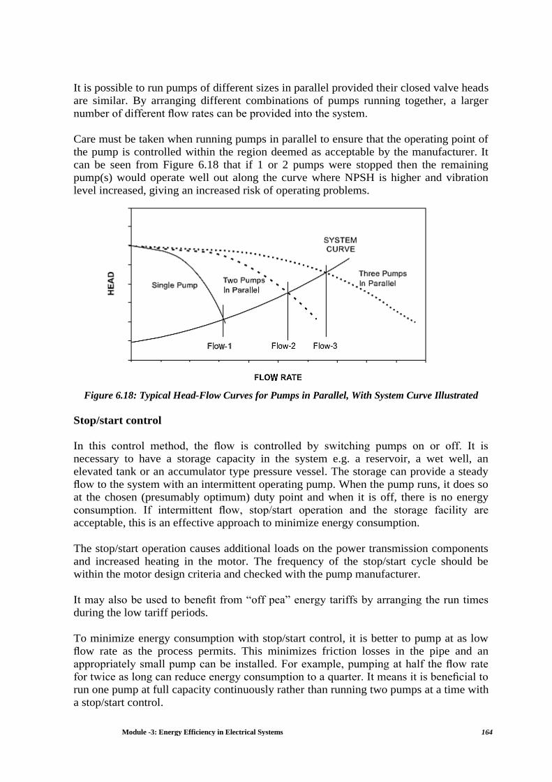
Module -3: Energy Efficiency in Electrical Systems 164
It is possible to run pumps of different sizes in parallel provided their closed valve heads
are similar. By arranging different combinations of pumps running together, a larger
number of different flow rates can be provided into the system.
Care must be taken when running pumps in parallel to ensure that the operating point of
the pump is controlled within the region deemed as acceptable by the manufacturer. It
can be seen from Figure 6.18 that if 1 or 2 pumps were stopped then the remaining
pump(s) would operate well out along the curve where NPSH is higher and vibration
level increased, giving an increased risk of operating problems.
Figure 6.18: Typical Head-Flow Curves for Pumps in Parallel, With System Curve Illustrated
Stop/start control
In this control method, the flow is controlled by switching pumps on or off. It is
necessary to have a storage capacity in the system e.g. a reservoir, a wet well, an
elevated tank or an accumulator type pressure vessel. The storage can provide a steady
flow to the system with an intermittent operating pump. When the pump runs, it does so
at the chosen (presumably optimum) duty point and when it is off, there is no energy
consumption. If intermittent flow, stop/start operation and the storage facility are
acceptable, this is an effective approach to minimize energy consumption.
The stop/start operation causes additional loads on the power transmission components
and increased heating in the motor. The frequency of the stop/start cycle should be
within the motor design criteria and checked with the pump manufacturer.
It may also be used to benefit from “off pea” energy tariffs by arranging the run times
during the low tariff periods.
To minimize energy consumption with stop/start control, it is better to pump at as low
flow rate as the process permits. This minimizes friction losses in the pipe and an
appropriately small pump can be installed. For example, pumping at half the flow rate
for twice as long can reduce energy consumption to a quarter. It means it is beneficial to
run one pump at full capacity continuously rather than running two pumps at a time with
a stop/start control.

Module -3: Energy Efficiency in Electrical Systems 165
Flow control valve
With this control method, the pump runs continuously and a valve in the pump
discharge line is opened or closed to adjust the flow to the required value.
Figure 6.19: Control of Pump Flow by Changing System Resistance Using 3 Valve.
To understand how the flow rate is controlled, see Figure 6.19. With the valve fully
open, the pump operates at “Flow 1”. When the valve is partially closed, it introduces an
additional friction loss in the system which is proportional to flow squared. The new
system curve cuts the pump curve at “Flow 2” which is the new operating point. The
head difference between the two curves is the pressure drop across the valve.
It is usual practice with valve control to have the valve 10% shut even at maximum
flow. Energy is therefore wasted overcoming the resistance through the valve at all flow
conditions. There is some reduction in pump power absorbed at the lower flow rate (see
Figure 6.19), but the flow multiplied by the head drop across the valve, is wasted
energy. It should also be noted that while the pump will accommodate changes in its
operating point as far as it is able within its performance range, it can be forced to
operate high on the curve where its efficiency is low and its reliability is affected.
Maintenance cost of control valves can be high, particularly on corrosive and solids-
containing liquids. Therefore, the lifetime cost could be unnecessarily high.
By-pass control
With this control approach, the pump runs continuously at the maximum process
demand duty with a permanent by-pass line attached to the outlet. When a lower flow is
required the surplus liquid is bypassed and returned to the supply source.

Module -3: Energy Efficiency in Electrical Systems 166
An alternative configuration may have a tank supplying a varying process demand,
which is kept full by a fixed duty pump running at the peak flow rate. Most of the time,
the tank overflows and recycles back to the pump suction. This is even less energy
efficient than a control valve because there is no reduction in power consumption with
reduced process demand.
The small by-pass line sometimes installed to prevent a pump running at zero flow is not
a means of flow control, but required for the safe operation of the pump.
Fixed Flow reduction
Impeller trimming
Impeller trimming refers to the process of machining the diameter of an impeller to
reduce the energy added to the system liquid.
Impeller trimming offers a useful correction to pumps that, through overly conservative
design practices or changes in system loads are oversized for their application.
Trimming an impeller provides a level of correction below buying a smaller impeller
from the pump manufacturer. But in many cases, the next smaller size impeller is too
small for the pump load. Also, smaller impellers may not be available for the pump size
in question and impeller trimming is the only practical alternative short of replacing the
entire pump/motor assembly. (See Figures 6.20 & 6.21 for before and after impeller
trimming).
Figure 6.20 Before Impeller Trimming Figure 6.21 After Impeller Trimming
Impeller trimming reduces tip speed which in turn directly lowers the amount of energy
imparted to the system liquid and lowers both the flow and pressure generated by the
pump.
The Affinity Laws, which describe centrifugal pump performance, provide a theoretical
relationship between impeller size and pump output (assuming constant pump speed):
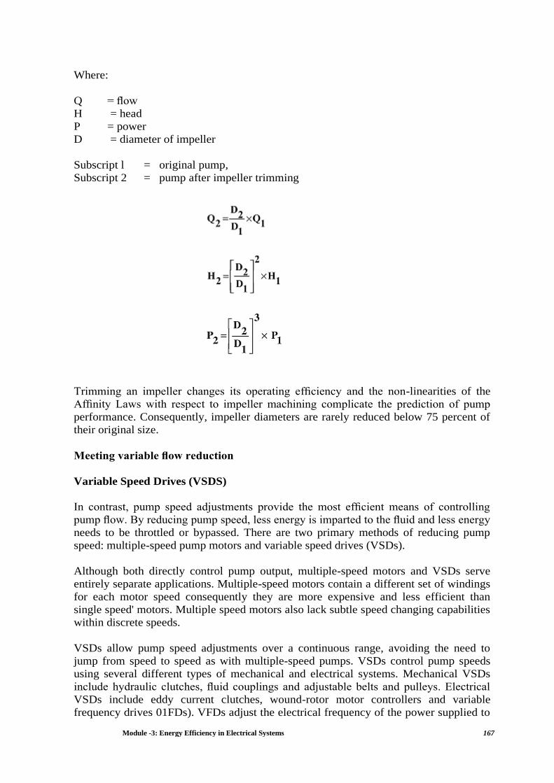
Module -3: Energy Efficiency in Electrical Systems 167
Where:
Q = flow
H = head
P = power
D = diameter of impeller
Subscript l = original pump,
Subscript 2 = pump after impeller trimming
Trimming an impeller changes its operating efficiency and the non-linearities of the
Affinity Laws with respect to impeller machining complicate the prediction of pump
performance. Consequently, impeller diameters are rarely reduced below 75 percent of
their original size.
Meeting variable flow reduction
Variable Speed Drives (VSDS)
In contrast, pump speed adjustments provide the most efficient means of controlling
pump flow. By reducing pump speed, less energy is imparted to the fluid and less energy
needs to be throttled or bypassed. There are two primary methods of reducing pump
speed: multiple-speed pump motors and variable speed drives (VSDs).
Although both directly control pump output, multiple-speed motors and VSDs serve
entirely separate applications. Multiple-speed motors contain a different set of windings
for each motor speed consequently they are more expensive and less efficient than
single speed' motors. Multiple speed motors also lack subtle speed changing capabilities
within discrete speeds.
VSDs allow pump speed adjustments over a continuous range, avoiding the need to
jump from speed to speed as with multiple-speed pumps. VSDs control pump speeds
using several different types of mechanical and electrical systems. Mechanical VSDs
include hydraulic clutches, fluid couplings and adjustable belts and pulleys. Electrical
VSDs include eddy current clutches, wound-rotor motor controllers and variable
frequency drives 01FDs). VFDs adjust the electrical frequency of the power supplied to
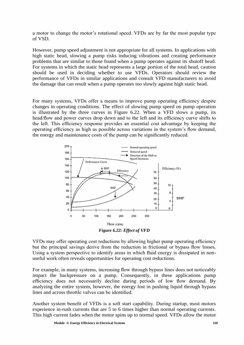
Module -3: Energy Efficiency in Electrical Systems 168
a motor to change the motor’s rotational speed. VFDs are by far the most popular type
of VSD.
However, pump speed adjustment is not appropriate for all systems. In applications with
high static head, slowing a pump risks inducing vibrations and creating performance
problems that are similar to those found when a pump operates against its shutoff head.
For systems in which the static head represents a large portion of the total head, caution
should be used in deciding whether to use VFDs. Operators should review the
performance of VFDs in similar applications and consult VFD manufacturers to avoid
the damage that can result when a pump operates too slowly against high static head.
For many systems, VFDs offer a means to improve pump operating efficiency despite
changes in operating conditions. The effect of slowing pump speed on pump operation
is illustrated by the three curves in Figure 6.22. When a VFD slows a pump, its
head/flow and power curves drop down and to the left and its efficiency curve shifts to
the left. This efficiency response provides an essential cost advantage by keeping the
operating efficiency as high as possible across variations in the system’s flow demand,
the energy and maintenance costs of the pump can be significantly reduced.
Figure 6.22: Effect of VFD
VFDs may offer operating cost reductions by allowing higher pump operating efficiency
but the principal savings derive from the reduction in frictional or bypass flow losses.
Using a system perspective to identify areas in which fluid energy is dissipated in non-
useful work often reveals opportunities for operating cost reductions.
For example, in many systems, increasing flow through bypass lines does not noticeably
impact the backpressure on a pump. Consequently, in these applications pump
efficiency does not necessarily decline during periods of low flow demand. By
analyzing the entire system, however, the energy lost in pushing liquid through bypass
lines and across throttle valves can be identified.
Another system benefit of VFDs is a soft start capability. During startup, most motors
experience in-rush currents that are 5 to 6 times higher than normal operating currents.
This high current fades when the motor spins up to normal speed. VFDs allow the motor

Module -3: Energy Efficiency in Electrical Systems 169
to be started with a lower startup current (usually only about 1.5 times the normal
operating current). This reduces wear on the motor and its controller. VFDs will
consume 4 to 6% power as a running cost apart from its initial cost.
6.7 Boiler Feed Water Pumps (BFP)
The feed water pumps are normally multi stage centrifugal pumps, sized based on boiler
design pressure. The operation of a multistage pump is similar to the operation of
several single stage pumps, of identical capacity, in series. Since most boilers operate
below design pressure, the feed water pump head is often higher than required. This
excessive pump head is dropped across pressure reducing valves and manual valves.
Installing a VFD on the feed water pump in such cases can decrease pump power
consumption and improve control performance. Trimming the impeller, reducing
number of stages or changing the feed water pumps may also be feasible depending on
variation in operating load of the boiler.
Boiler Feed Pump Control with VFD
There are several ways of controlling the pump
One pump, one boiler, no feed water regulating valve: In this the pump speed
is varied according to the level of water in the boiler. The level control system
used for the feed water admission valve transmits its signal directly to the pump
VFD controller. With this system it is possible to eliminate not only the feed
pump constant discharge but also the boiler feed water regulating control valve
and, thereby, cut initial capital investment. The inherent efficiency loss due to
throttling is eliminated.
Constant discharge pressure control: The feed pump is controlled to a
predetermined pressure setting irrespective of plant load. The advantage of this
system is that the pump will not be required to operate near shut off pressures,
due to the shifting of the operating point on the curve.
Constant differential pressure control: Feed pump pressure is controlled to
produce a predetermined pressure drop across the feed water regulating valve,
usually approximately 3.5 to 5.5 kg/cm2, thus allowing the boiler feed pump to
follow plant demand.
Optimizing Boiler Feed Water Pump Capacity - Case
A waste heat boiler has two feed water pumps, each of 6 stages and having a capacity of
35 m3/hr. The pumps are designed to generate a head of 276 m, normally one pump is
operated.
The actual steam demand is 28 TPH at 15 kg/cm2. The capacity of the feed water pumps
is far in excess of the requirement. This results in throttling of pump discharge leading
to energy loss. To save energy in the BFW pumps, it was suggested to remove two
impeller stages of the pump to effectively regulate the pressure developed in the pumps.
The impact of this measure on power consumption was then evaluated and the results
are given in Table 6.2:
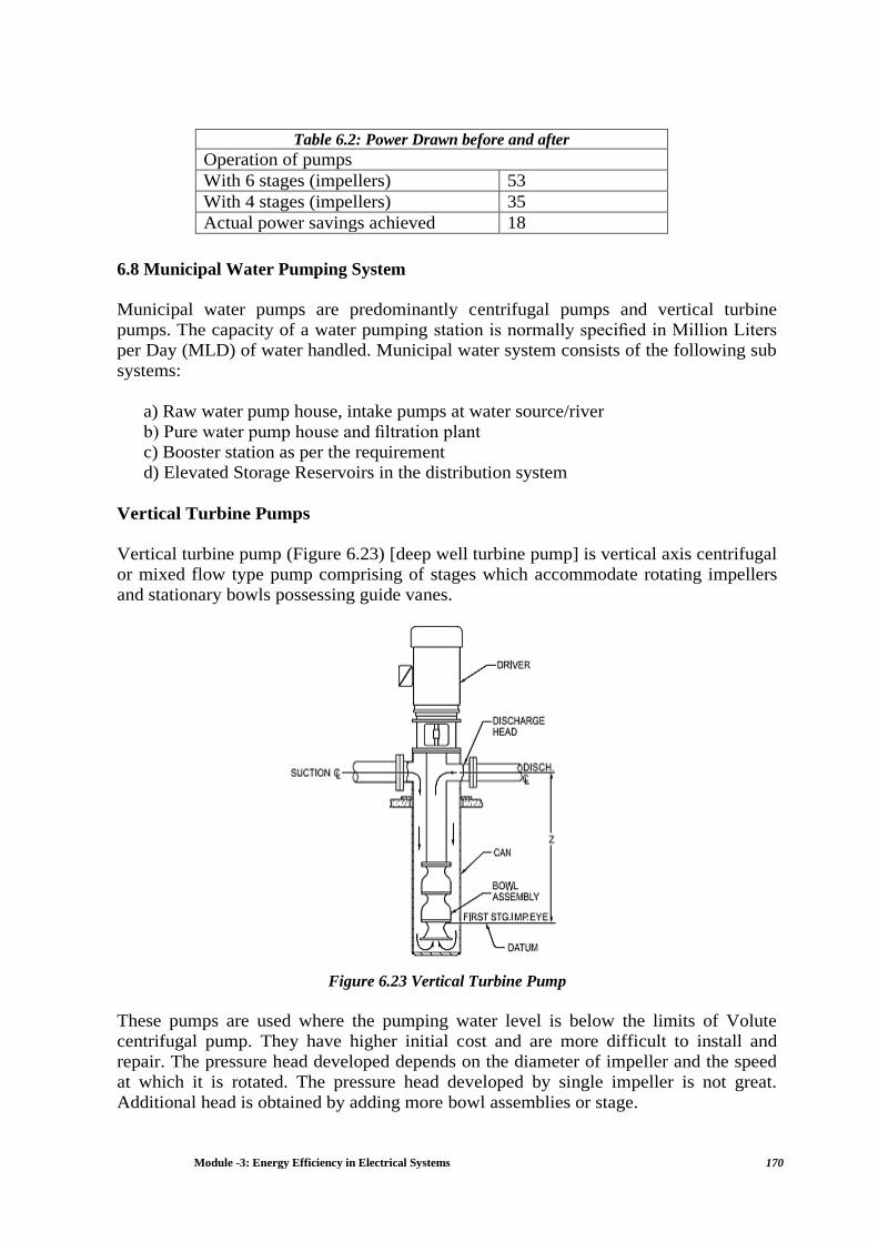
Module -3: Energy Efficiency in Electrical Systems 170
Table 6.2: Power Drawn before and after
Operation of pumps
With 6 stages (impellers) 53
With 4 stages (impellers) 35
Actual power savings achieved 18
6.8 Municipal Water Pumping System
Municipal water pumps are predominantly centrifugal pumps and vertical turbine
pumps. The capacity of a water pumping station is normally specified in Million Liters
per Day (MLD) of water handled. Municipal water system consists of the following sub
systems:
a) Raw water pump house, intake pumps at water source/river
b) Pure water pump house and filtration plant
c) Booster station as per the requirement
d) Elevated Storage Reservoirs in the distribution system
Vertical Turbine Pumps
Vertical turbine pump (Figure 6.23) [deep well turbine pump] is vertical axis centrifugal
or mixed flow type pump comprising of stages which accommodate rotating impellers
and stationary bowls possessing guide vanes.
Figure 6.23 Vertical Turbine Pump
These pumps are used where the pumping water level is below the limits of Volute
centrifugal pump. They have higher initial cost and are more difficult to install and
repair. The pressure head developed depends on the diameter of impeller and the speed
at which it is rotated. The pressure head developed by single impeller is not great.
Additional head is obtained by adding more bowl assemblies or stage.

Module -3: Energy Efficiency in Electrical Systems 171
Construction:
It has three parts:
1. Pump Element:
The pump element is made up of one or more bowls or stages. Each bowl consists of an
impeller and diffuser.
2. Discharge Column:
It connects the bowl assembly and pump head and conducts water from former to later.
Discharge head:
It consists of base from which the discharge column, bowl assembly and shaft assembly
are suspended.
Submersible Pump:
A vertical turbine pump close coupled to a small diameter submersible electric motor is
termed as “submersible pump”. The motor is fixed directly below the intake of the
pump. The pump element and the motor operate under submerged condition. It can be
used in very deep tube well where a long shaft would not be practical.
6.9 Sewage Water Pumps
The fundamental difference between a centrifugal sewage pump impeller and those of
clear water pumps is its ability to pass solid material that would normally clog the latter.
What differentiates various sewage pump impellers is the method by which they
accomplish this. All sewage handling pumps comprise single suction impellers. This is
to avoid the necessity of locating the pump shaft in the intake.
The Figure 6.24 is that of a typical radial flow impeller of a pump used to handle coarse
solids or fibrous matters. These pumps use volutes because diffuser is prone to clogging.
The design of sewage pumps is largely determined by the size of foreign matter that
must pass through the pump without clogging.
Figure 6.24 Radial Flow Impeller

Module -3: Energy Efficiency in Electrical Systems 172
6.10 Agricultural Pumping System
The pumps used in agriculture sector are normally installed by individual farmers based
on the guidelines provided by agriculture department/state utilities and feedback from
other users. Most of the pumps used are locally manufactured keeping initial investment
as the selection criteria rather than efficiency and energy conservation.
The pump sets used are generally inefficient with operating efficiency ranging from 30 -
55%. The wide variation is due to changing water levels in the intake thus forcing the
pump to operate away from the best efficiency point. The pump sets are more often
oversized so as to draw water from increasingly declining depths and also to withstand
large voltage fluctuations.
Mostly centrifugal pumps are used and the capacity of the pumps vary from 1 Hp to 25
Hp. The rating of the pumps is decided based on water table levels. High rating pumps
above 25 HP are also used in several areas. Large capacity centrifugal pumps of 75 HP
to 500 HP ratings are also used by Irrigation departments to provide water to
agricultural consumers. Diesel engine driven pumps are also common in areas where
there is erratic or no power supply.
The following energy conservation opportunities have been demonstrated for energy
savings in agricultural pumping.
Installation of low friction foot valves
Installation of low friction HDPE suction and delivery pipes
Installation of long bends
Installation of high efficiency pumps and motors
6.11 Energy Conservation Opportunities in Pumping Systems
Ensure adequate NPSH at site of installation.
Ensure availability of basic instruments at pumps like pressure gauges, flow
meters.
Operate pumps near Best Efficiency Point.
Modify pumping system and pumps losses to minimize throttling.
Adapt to wide load variation with variable speed drives or sequenced control of
multiple units.
Stop running multiple pumps - add an auto-start for an on-line spare or add a
booster pump in the problem area.
Use booster pumps for small loads requiring higher pressures.
Increase liquid temperature differentials to reduce pumping rates in case of heat
exchangers.
Decrease outlet cold water temperature of cooling tower in order to reduce the
pumping flow rates in case of mixing.
Separate High Pressure and Low Pressure systems
Repair seals and packing to minimize water loss by dripping.
Balance the system to minimize flows and reduce pump power requirements.
Avoid pumping head with a free-fall return (gravity); Use siphon effect to
advantage:
Conduct water balance to minimize water consumption.

Module -3: Energy Efficiency in Electrical Systems 173
Avoid cooling water re-circulation in DG sets, air compressors, refrigeration
systems, cooling towers feed water pumps, condenser pumps and process pumps.
In multiple pump operations, carefully combine the operation of pumps to avoid
throttling.
Provide booster pump for few areas of higher head.
Replace old pumps by energy efficient pumps.
In the case of over designed pump, provide variable speed drive, or downsize /
replace impeller or replace with correct sized pump for efficient operation.
Optimize number of stages in multi-stage pump in case of head margins.
Reduce system resistance by pressure drop assessment and pipe size
optimization.
Example 6.1
The cooling water circuit of a process industry is depicted in the figure below. Cooling
water is pumped to three heat exchangers via pipes A, B and C where flow is throttled
depending upon the requirement. The diameter of pipes and measured velocities with
non-contact ultrasonic flow meter in each pipe are indicated in the figure.
The following are the other data:
Measured motor power : 50.7 kW
Motor efficiency at operating load : 90%
Pump discharge pressure : 3.4 kg/cm2
Suction head : 2 meters
Determine the efficiency of the pump.
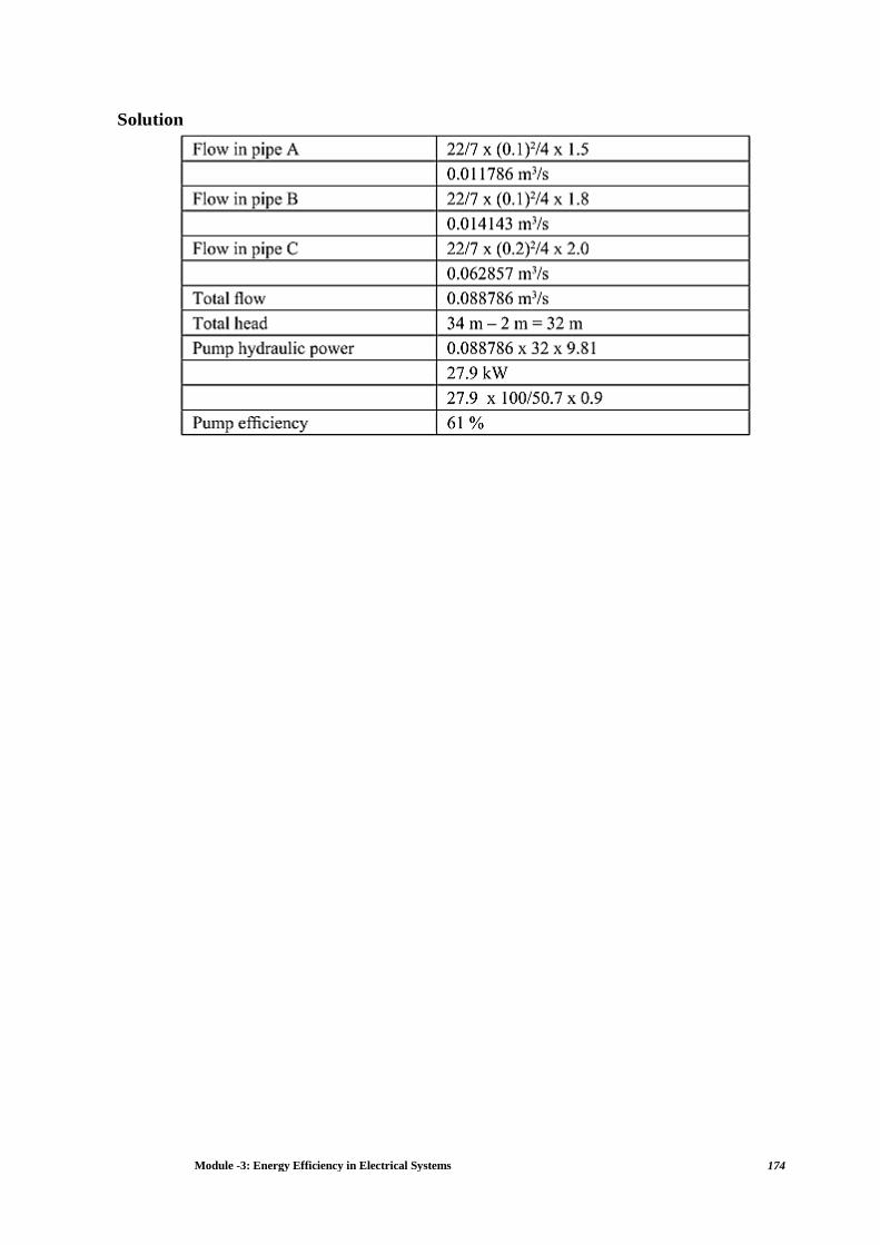
Module -3: Energy Efficiency in Electrical Systems 174
Solution

Module -3: Energy Efficiency in Electrical Systems 175
Chapter 7: COOLING TOWER
7.1 Introduction
Cooling towers are a very important part of many chemical plants. The primary task of a
cooling tower is to reject heat into the atmosphere. They represent a relatively
inexpensive and dependable means of removing low-grade heat from cooling water. The
make-up water source is used to replenish water lost to evaporation. Hot water from
heat exchangers is sent to the cooling tower. The water exits the cooling tower and is
sent back to the exchangers or to other units for further cooling. Typical closed loop
cooling tower system is shown in Figure 7.1.
Figure 7.1 Cooling Water System
Cooling Tower Types
Cooling towers fall into two main categories: Natural draft and Mechanical draft.
Natural draft towers use very large concrete chimneys to introduce air through the
media. Due to the large size of these towers, they are generally used for water flow rates
above 45,000 m3/hr. These types of towers are used only by utility power stations.
Mechanical draft towers utilize large fans to force or suck air through circulated water.
The water falls downward over fill surfaces, which help increase the contact time
between the water and the air – this helps maximise heat transfer between the two.
Cooling rates of Mechanical draft towers depend upon their fan diameter and speed of
operation. Since, the mechanical draft cooling towers are much more widely used; the
focus is on them in this chapter.
Mechanical draft towers
Mechanical draft towers are available in the following airflow arrangements:
1. Counter flows induced draft.
2. Counter flow forced draft.
3. Cross flow induced draft.

Module -3: Energy Efficiency in Electrical Systems 176
In the counter flow induced draft design, hot water enters at the top, while the air is
introduced at the bottom and exits at the top. Both forced and induced draft fans are
used.
In cross flow induced draft towers, the water enters at the top and passes over the fill.
The air, however, is introduced at the side either on one side (single-flow tower) or
opposite sides (double-flow tower). An induced draft fan draws the air across the wetted
fill and expels it through the top of the structure.
The Figure 7.2 illustrates various cooling tower types. Mechanical draft towers are
available in a large range of capacities. Normal capacities range from approximately 10
tons, 2.5 m3/hr flow to several thousand tons and m3/hr. Towers can be factory built or
field erected -for example concrete towers are only field erected.
Many towers are constructed so that they can be grouped together to achieve the desired
capacity. Thus, many cooling towers are assemblies of two or more individual cooling
towers or “cells.” The number of cells they have, e.g., a eight-cell tower, often refers to
such towers. Multiple-cell towers can be lineal, square, or round depending upon the
shape of the individual cells and whether the air inlets are located on the sides or
bottoms of the cells.
Components of Cooling Tower
The basic components of an evaporative tower are: Frame and casing, fill, cold water
basin, drift eliminators, air inlet, louvers, nozzles and fans.
Frame and easing: Most towers have structural frames that support the exterior
enclosures (casings), motors, fans, and other components. With some smaller designs,
such as some glass fiber units, the casing may essentially be the frame.
Fill: Most towers employ fills (made of plastic or wood) to facilitate heat transfer by
maximising water and air contact. Fill can either be splash or film type.
With splash fill, water falls over successive layers of horizontal splash bars,
continuously breaking into smaller droplets, while also wetting the fill surface. Plastic
splash fill promotes better heat transfer than the wood splash fill.
Film fill consists of thin, closely spaced plastic surfaces over which the water spreads,
forming a thin film in contact with the air. These surfaces may be flat, corrugated,
honeycombed, or other patterns. The film type of fill is the more efficient and provides
same heat transfer in a smaller volume than the splash fill.
Cold water basin: The cold water basin, located at or near the bottom of the tower,
receives the cooled water that flows down through the tower and fill. The basin usually
has a sump or low point for the cold water discharge connection. In many tower designs,
the cold water basin is beneath the entire fill.

Module -3: Energy Efficiency in Electrical Systems 177
Figure 7.2 Cooling Tower Types
In some forced draft counter flow design, however, the water at the bottom of the fill is
channeled to a perimeter trough that functions as the cold water basin. Propeller fans are
mounted beneath the fill to blow the air up through the tower. With this design, the
tower is mounted on legs, providing easy access to the fans and their motors.
Drift eliminators:
These capture water droplets entrapped in the air stream that otherwise would be lost to
the atmosphere.
Air inlet: This is the point of entry for the air entering a tower. The inlet may take up an
entire side of a tower-cross flow design-or be located low on the side or the bottom of
counter flow designs.
Louvers: Generally, cross-flow towers have inlet louvers. The purpose of louvers is to
equalize air flow into the fill and retain the water within the tower. Many counter flow
tower designs do not require louvers.
Nozzles: These provide the water sprays to wet the fill. Uniform water distribution at
the top of the fill is essential to achieve proper wetting of the entire fill surface. Nozzles

Module -3: Energy Efficiency in Electrical Systems 178
can either be fixed in place and have either round or square spray patterns or can be part
of a rotating assembly as found in some circular cross-section towers.
Fans: Both axial (propeller type) and centrifugal fans are used in towers. Generally,
propeller fans are used in induced draft towers and both propeller and centrifugal fans
are found in forced draft towers. Depending upon their size, propeller fans can either be
fixed or variable pitch. A fan having non-automatic adjustable pitch blades permits the
same fan to be used over a wide range of kW with the fan adjusted to deliver the desired
air flow at the lowest power consumption.
Automatic variable pitch blades can vary air flow in response to changing load
conditions.
Tower Materials
In the early days of cooling tower manufacture, towers were constructed primarily of
wood. Wooden components included the frame, casing, louvers, fill, and often the cold
water basin. If the basin was not of wood, it likely was of concrete.
Today, tower manufacturers fabricate towers and tower components from a variety of
materials. Often several materials are used to enhance corrosion resistance, reduce
maintenance, and promote reliability and long service life. Galvanized steel, various
grades of stainless steel, glass fiber, and concrete are widely used in tower construction
as well as aluminum and various types of plastics for some components.
Wood towers are still available, but they have glass fiber rather than wood panels
(casing) over the wood framework. The inlet air louvers may be glass fiber, the fill may
be plastic, and the cold water basin may be steel.
Larger towers sometimes are made of concrete. Many towers—casings and basins—are
constructed of galvanized steel or, where a corrosive atmosphere is a problem, stainless
steel. Sometimes a galvanized tower has a stainless steel basin. Glass fiber is also widely
used for cooling tower casings and basins, giving long life and protection from the
harmful effects of many chemicals.
Plastics are widely used for fill, including PVC, polypropylene, and other polymers.
Treated wood splash fill is still specified for wood towers, but plastic splash fill is also
widely used when water conditions mandate the use of splash fill. Film fill, because it
offers greater heat transfer efficiency, is the fill of choice for applications where the
circulating water is generally free of debris that could plug the fill passageways.
Plastics also find wide use as nozzle materials. Many nozzles are being made of PVC,
ABS, polypropylene, and glass-filled nylon. Aluminum, glass fiber, and hot-dipped
galvanized steel are commonly used fan materials. Centrifugal fans are often fabricated
from galvanized steel. Propeller fans are fabricated from galvanized, aluminum, or
molded glass fiber reinforced plastic.
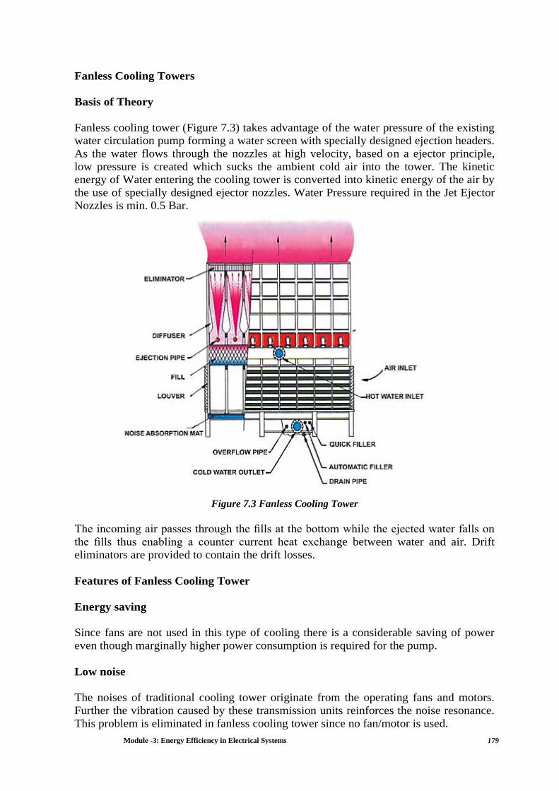
Module -3: Energy Efficiency in Electrical Systems 179
Fanless Cooling Towers
Basis of Theory
Fanless cooling tower (Figure 7.3) takes advantage of the water pressure of the existing
water circulation pump forming a water screen with specially designed ejection headers.
As the water flows through the nozzles at high velocity, based on a ejector principle,
low pressure is created which sucks the ambient cold air into the tower. The kinetic
energy of Water entering the cooling tower is converted into kinetic energy of the air by
the use of specially designed ejector nozzles. Water Pressure required in the Jet Ejector
Nozzles is min. 0.5 Bar.
Figure 7.3 Fanless Cooling Tower
The incoming air passes through the fills at the bottom while the ejected water falls on
the fills thus enabling a counter current heat exchange between water and air. Drift
eliminators are provided to contain the drift losses.
Features of Fanless Cooling Tower
Energy saving
Since fans are not used in this type of cooling there is a considerable saving of power
even though marginally higher power consumption is required for the pump.
Low noise
The noises of traditional cooling tower originate from the operating fans and motors.
Further the vibration caused by these transmission units reinforces the noise resonance.
This problem is eliminated in fanless cooling tower since no fan/motor is used.

Module -3: Energy Efficiency in Electrical Systems 180
Water saving
The velocity of water is less than that in conventional cooling tower. In combination
with high efficiency drift eliminators this can reduce the drift loss to 0.001% which is
much less than that for a conventional tower. Since the water droplets will be less than
50 micron it evaporates immediately without causing any pollution nearby.
Low maintenance cost
Since the fanless cooling tower has no mechanical equipment such as fan, motor,
gearbox etc. there is hardly any maintenance required, provided the quality of
circulation water is kept clean and well maintained.
7.2 Cooling Tower Performance
The important parameters, from the point of determining the performance of cooling
towers, are:
Figure 7.4 Range and Approach
i. “Range” is the difference between the cooling tower water inlet and outlet
temperature. (see Figure 7.4).
ii. “Approach” is the difference between the cooling tower outlet cold water
temperature and ambient wet bulb temperature. Although, both range and
approach should be monitored, the ‘Approach’ is a better indicator of cooling
tower performance. (see Figure 7 .4).
iii. Cooling tower effectiveness (in percentage) is the ratio of range, to the ideal
range, i.e., difference between cooling water inlet temperature and ambient wet
bulb temperature, or in other words it is = Range / (Range + Approach).
iv. Cooling capacity is the heat rejected in kcal/hr or TR, given as product of mass
flow rate of water, specific heat and temperature difference

Module -3: Energy Efficiency in Electrical Systems 181
v. Evaporation loss is the water quantity evaporated for cooling duty and,
theoretically, for every 10, 00,000 kcal heat rejected, evaporation quantity works
out to 1.8 m3. An empirical relation used often is:
*Evaporation Loss (m3/hr) = 0.00085 x 1.8 x circulation rate (m3/hr) x (T1-T2)
Tl -T2 = Temperature difference between inlet and outlet water.
*Source: Perry’s Chemical Engineers Handbook (Page: 12-17)
vi. Cycles of concentration (CDC) is the ratio of dissolved solids in circulating
water to the dissolved solids in makeup water.
Blow Down = Evaporation Loss / (C.O.C. - 1)
vii. Liquid/Gas (L/G) ratio, of a cooling tower is the ratio between the water and the
air mass flow rates. Against design values, seasonal variations require adjustment
and tuning of water and air flow rates to get the best cooling tower effectiveness
through measures like water box loading changes, blade angle adjustments.
Thermodynamics also dictate that the heat removed from the water must be equal to the
heat absorbed by the surrounding air:
L (T1 –T2) = G (h2 – h1)
Where,
L/G = liquid to gas mass flow ratio (kg/kg)
T1 = hot water temperature (0C)
T2 = cold water temperature (0C)
h2 = enthalpy of air-water vapor mixture at exhaust wet-bulb
temperature
(same units as above)
h1 = enthalpy of air-water vapor mixture at inlet wet-bulb
temperature
(same units as above)
Factors Affecting Cooling Tower Performance
Capacity
Heat dissipation (in kcal/hour) and circulated flow rate (m3/hr) are not sufficient to
understand cooling tower performance. Other factors, which we will see, must be stated
along with flow rate m3/hr. For example, a cooling tower sized to cool 4540 m3/hr
through a 13.9°C range might be larger than a cooling tower to cool 4540 m3/hr through
19.5°C range.

Module -3: Energy Efficiency in Electrical Systems 182
Range
Range is determined not by the cooling tower, but by the process it is serving. The range
at the exchanger is determined entirely by the heat load and the water circulation rate
through the exchanger and on to the cooling water.
Range OC = Heat Load in kcaUhour / Water Circulation Rate in LPH
As a generalization, the closer the approach to the wet bulb, the more expensive the
cooling tower due to increased size. Usually a 2.8°C approach to the design wet bulb is
the coldest water temperature that cooling tower manufacturers will guarantee. If flow
rate, range, approach and wet bulb had to be ranked in the order of their importance in
sizing a tower, approach would be first with flow rate closely following the range and
wet bulb would be of lesser importance.
Heat Load
The heat load imposed on a cooling tower is determined by the process being served.
The degree of cooling required is controlled by the desired operating temperature level
of the process. In most cases, a low operating temperature is desirable to increase
process efficiency or to improve the quality or quantity ofthe product. In some
applications (e. g. internal combustion engines), however, high operating temperatures
are desirable. The size and cost of the cooling tower is proportional to the heat load. If
heat load calculations are low undersized equipment will be purchased. If the calculated
load is high, oversize and more costly, equipment will result.
Process heat loads may vary considerably depending upon the process involved.
Determination of accurate process heat loads can become very complex but proper
consideration can produce satisfactory results. On the other hand, air conditioning and
refrigeration heat loads can be determined with greater accuracy.
Information is available for the heat rejection requirements of various types of power
equipment. A sample list is as follows:
Air Compressor
- Single-stage - 129 kcal/kW/hr
- Single-stage with after cooler - 862 kcal/kW/hr
- Two-stage with intercooler - 518 kcal/kW/hr
- Two-stage with intercooler and after cooler - 862 kcal/kW/hr

Module -3: Energy Efficiency in Electrical Systems 183
Refrigeration, Compression - 63 kcal/min/TR
Refrigeration, Absorption - 127 kcal/min/TR
Steam Turbine Condenser - 555 kcal/kg of steam
Diesel Engine, Four-Cycle, Supercharged - 880 kcal/kW/hr
Natural Gas Engine, Four-cycle - 1523 kcal/kW/hr
(l8 kg/cm2 compression)
Wet Bulb Temperature
Wet bulb temperature is an important factor in performance of evaporative water
cooling equipment.
It is a controlling factor from the aspect of minimum cold water temperature to which
water can be cooled by the evaporative method. Thus, the wet bulb temperature of the
air entering the cooling tower determines operating temperature levels throughout the
plant, process, or system. Theoretically, a cooling tower will cool water to the entering
wet bulb temperature, when operating without a heat load. However, a thermal potential
is required to reject heat, so it is not possible to cool water to the entering air wet bulb
temperature, when a heat load is applied. The approach obtained is a function of thermal
conditions and tower capability.
Initial selection of towers with respect to design wet bulb temperature must be made on
the basis of conditions existing at the tower site. The temperature selected is generally
close to the average maximum wet bulb for the summer months. An important aspect of
wet bulb selection is, whether it is specified as ambient or inlet. The ambient wet bulb is
the temperature, which exists generally in the cooling tower area, whereas inlet wet bulb
is the wet bulb temperature of the air entering the tower. The later can be, and often is,
affected by discharge vapors being recalculated into the tower. Recirculation raises the
effective wet bulb temperature of the air entering the tower with corresponding increase
in the cold water temperature. Since there is no initial knowledge or control over the
recirculation factor, the ambient wet bulb should be specified. The cooling tower
supplier is required to furnish a tower of sufficient capability to absorb the effects of the
increased wet bulb temperature peculiar to his own equipment.
It is very important to have the cold water temperature low enough to exchange heat or
to condense vapours at the optimum temperature level. By evaluating the cost and size
of heat exchangers versus the cost and size of the cooling tower, the quantity and
temperature of the cooling tower water can be selected to get the maximum economy for
the particular process.
The Table 7. 1 illustrates the effect of approach on the size and cost of a cooling tower.
The towers included were sized to cool 4540 m3/hr through a 16.67°C range at a 267°C
design wet bulb. The overall width of all towers is 21.65 meters; the overall height, 15
.25 meters, and the pump head, 10.6 m approximately.

Module -3: Energy Efficiency in Electrical Systems 184
Table- 7.1: Approach VS Cooling Tower Size (4540 m3 /hr; 16.67oC Range; 26.7 oC Wet bulb; 10.
7 Pump Head)
Approach and Flow
Suppose a cooling tower is installed that is 21.65 m wide x 36.9 m long x 15.24 m high,
has three 7.32m diameter fans and each powered by 25 kW motors. The cooling tower
cools from 3632 m3/hr water from 461°C to 294°C at 26.7°C WBT dissipating 60.69
million kcal/hr. The Table 7.2 shows what would happen with additional flow but with
the range remaining constant at 16.67°C. The heat dissipated varies from 60.69 million
kcal/hr to 271.3 million kcal/hr.
Table 7.2 Flow vs. Approach for a Given Tower (Tower is 21.65 m x 36.9 M; Three 7.32 M Fans;
Three 25 kw Motor; 16.7°C Range with 26.7°C Wet Bulb)
For meeting the increased heat load, few modifications would be needed to increase the
water flow through the tower. However, at higher capacities, the approach would
increase.
Range, Flow and Heat Load
Range is a direct function of the quantity of water circulated and the heat load.
Increasing the range as a result of added heat load does require an increase in the tower
size. If the cold water temperature is not changed and the range is increased with higher
hot water temperature, the driving force between the wet bulb temperature of the air

Module -3: Energy Efficiency in Electrical Systems 185
entering the tower and the hot water temperature is increased, the higher level heat is
economical to dissipate.
If the hot water temperature is left constant and the range is increased by specifying a
lower cold water temperature, the tower size would have to be increased considerably.
Not only would the range be increased, but the lower cold water temperature would
lower the approach. The resulting change in both range and approach would require a
much larger cooling tower.
Approach & Wet Bulb Temperature
The design wet bulb temperature is determined by the geographical location. Usually
the design wet bulb temperature selected is not exceeded over 5 percent of the time in
that area. Wet bulb temperature is a factor in cooling tower selection; the higher the wet
bulb temperature, the smaller the tower required to give a specified approach to the wet
bulb at a constant range and flow rate.
A 4540 m3/hr cooling tower selected for a 16.67°C range and a 4.45°C approach to
21.11°C wet bulb would be larger than a 4540 m3/hr tower selected for a 16.67°C range
and a 4.45°C approach to a
26.67°C wet bulb. Air at the higher wet bulb temperature is capable of picking up more
heat. Assume that the wet bulb temperature of the air is increased by approximately
11.1°C. As air removes heat from the water in the tower, each kg of air entering the
tower at 21.1°C wet bulb would contain 18.86 kcals and if it were to leave the tower at
322°C wet bulb it would contain 24.17 kcal per kg of air.
In the second case, each kg of air entering the tower at 26.67°C wet bulb would contain
24.17 kcal and were to leave at 378°C wet bulb it would contain 39.67 kcal per kg of
air.
In going from 21.10C to 32.2oC, 12.1 kcal per kg of air is picked up, while 15.5 kcal/kg
of air is picked up in going from 26.67°C to 37.8°C.
Fill Media Effects
In a cooling tower, hot water is distributed above fill media which flows down and is
cooled due to evaporation with the intermixing air. Air draft is achieved with use of
fans. Thus some power is consumed in pumping the water to a height above the fill and
also by fans creating the draft.
An energy efficient or low power consuming cooling tower is to have efficient designs
of fill media with appropriate water distribution, drift eliminator, fan, gearbox and
motor. Power savings in a cooling tower, with use of efficient fill design, is directly
reflected as savings in fan power consumption and pumping head requirement.
Function of Fill media in a Cooling Tower
Heat exchange between air and water is influenced by surface area of heat exchange,
time of heat exchange (interaction) and turbulence in water effecting thoroughness of
intermixing. Fill media in a cooling tower is responsible to achieve all of above.

Module -3: Energy Efficiency in Electrical Systems 186
Splash and Film Fill Media: As the name indicates, splash fill media generates the
required heat exchange area by splashing action of water over fill media and hence
breaking into smaller water droplets. Thus, surface of heat exchange is the surface area
of the water droplets, which is in contact with air.
Film Fill and its Advantages
In a film fill, water forms a thin film on either side of the fill sheets. Thus area of heat
exchange is the surface area of the fill sheets, which is in contact with air.
Typical comparison between various fill media is shown in Table 7.3.
Table 7.3. Comparisons between various fill media
Due to fewer requirements of air and pumping head, there is a tremendous saving in
power with the invention of film fill. Recently, low-clog film fills with higher flute sizes
have been developed to handle high turbid waters. For sea water, low clog film fills are
considered as the best choice in terms of power saving and performance compared to
conventional splash type fills.
Choosing a Cooling Tower
The counter-flow and cross flows are two basic designs of cooling towers based on the
fundamentals of heat exchange. It is well known that counter flow heat exchange is
more effective as compared to cross flow or parallel flow heat exchange.
Cross-flow cooling towers are provided with splash fill of concrete, wood or perforated
PVC. Counter-flow cooling towers are provided with both film fill and splash fill.
Typical comparison of Cross flow Splash Fill, Counter Flow Tower with Film Fill and
Splash fill is shown in Table 7.4. The power consumption is least in Counter Flow Film
Fill followed by Counter Flow Splash Fill and Cross-Flow Splash Fill.

Module -3: Energy Efficiency in Electrical Systems 187
Table 7.4: Typical Comparison of Cross flow splash fill, Counter Flow Tower with Film Fill and
Splash Fill
7.3 Efficient System Operation
i. Cooling Water Treatment
Cooling water systems is one of the Critical utility in Power plants, process industries
and in Air- conditioning systems. The power plant performance, Chiller performance
have direct effect on energy consumption, based on Cooling water temperatures which
in turn is maintained by good cooling water treatment.
The various problems in Cooling water system and the corrective measures required are
discussed below.
a) Water Side Problems
Usually the typical problems that any (Open) cooling system meets with are:
Corrosion and/or Scale formation
Biological/Micro-biological fouling
Corrosion:
Corrosion, being not a precisely understood phenomenon, is a function of various
factors of which the following are the main factors responsible for promoting corrosion
in the system; high salinity of the water, low PH, low Alkalinity, presence of corrosive
gases (mainly oxygen and C02), dissimilarity of the metals etc.
Corrosion can either lead to failure of the metallurgy (leakages in the heat exchangers)
and/or deposit formation of corrosion products.

Module -3: Energy Efficiency in Electrical Systems 188
Scale Formation:
The main sources for the scale formation in the Open Evaporative Condenser circuit are:
Hard water containing, high levels of Calcium and Magnesium, high level of PH and
Alkalinity. An open evaporative cooling systems (condenser water systems) operated on
softened water can meet with severe scaling problems when
PH of the circulating water is above 9.0
The total Alkalinity as CaCO3 is above 550 ppm
Temporary hardness in the sources of make-up is above 200 ppm
Biological/Micro—Biological Fouling
Systems exposed to sunlight (mainly cooling tower) often meet with severe problem of
algae formation. Other problems associated with algae are slime mass, fungi and various
species of bacteria.
Bacteria being miniature bodies, of which growth is not controlled, can lead to the
formation of fine masses of suspended particles that lead to fouling and deposit
formation. Algae obviously block the nozzles of the cooling tower and thus reduce
temperature drop across the tower. Slime masses again are responsible for fouling and
deposit formation.
Deposit Formation:
Foreign matter such as; turbidity, sand, silt, mud, air borne debris and other suspended
impurities are the sources of deposits formation. Corrosion products that are formed also
add to the deposit formation.
b) Energy Losses:
Regardless of the type of system, be it open or closed, if it meets with any of the above
problems, either the cooling tower nozzles are blocked resulting in reduced Delta ‘T’
and/or the deposits/scales are formed on the heat transfer surfaces.
For example, the energy losses due to scale and deposit formation in a cooling water
circuit of a refrigeration system are significant as shown in Table 7.5. The scale and
deposit on the heat transfer area in process equipment can also cause production loss.

Module -3: Energy Efficiency in Electrical Systems 189
Table7.5 Effect of Fouling on Efficiency and Power Consumption
c) Solution to the Problems
ON line / OFF Line Chemical Cleaning
Depending on the criticality the plant management may adopt ON line/ OFF line
cleaning systems.
Preventive Treatment
For preventive treatment, a wide range of chemicals are available in the market and
formulations manufactured by reputed companies are generally very safe to use in the
system.
Corrosion/Scale Inhibitors
To control corrosion and scale formation depending upon the severity of each of the
problem, either or both chemicals should be used and the selection of the chemicals
should be made in accordance with the quality of the make-up water available for plant
operation.
Dispersants (For Deposit Formation)
Suitable dispersants help in controlling the deposit formation and selection of the
dispersants is made in accordance with the nature of suspended solids/deposits forming
particulate present in the water.
Side Stream Filter
Circulating water having very high levels of turbidity and/or suspended impurities
should be facilitated with side stream filters. Side stream filters are generally selected to
handle 2% to 5% of the total rate of circulation, but to ensure that the total water content
in the system (hold-up volume) is filtered approximately once in 12 hours.
Bio Dispersants and Biocides
To combat problems arising due to the growth of biological and micro biological
species, such as algae, fungi, slime, bacteria etc. It is very essential to select a

Module -3: Energy Efficiency in Electrical Systems 190
combination of oxidizing and non- oxidizing biocides. Bio-dispersants are used to
remove the upper layer of the biological masses and allow better penetration of biocides
in the lower layers of bio-masses.
Chlorination
Chlorination is the most effective and most economical oxidizing biocide. Chlorination
for the smaller systems may be done with hypo chlorite based products and for the
larger systems having hold-up volume in excess of 100 m3 be done with suitable gas
chlorinators. The safest gas chlorination equipment are vacuum gravity feed type which
can be easily installed on either 50 kg or 100 kg chlorine cylinders.
ii. Drift Loss in the Cooling Towers
It is very difficult to ignore drift problem in cooling towers. Now-a—days most of the
end user specification calls for 0.02% drift loss. With technological development and
processing of PVC, manufacturers have brought large change in
the drift eliminator shapes and the possibility of making efficient designs of drift
eliminators that enable end user to specify the drift loss requirement to as low as 0.003
— 0.001%.
iii. Cooling Tower Fans
The purpose of a cooling tower fan is to move a specified quantity of air through the
system, overcoming the system resistance which is defined as the pressure loss. The
product of air flow and the pressure loss is air power developed/work done by the fan;
this may be also termed as fan output and input kW depends on fan efficiency.
The fan efficiency in turn is greatly dependent on the profile of the blade. An
aerodynamic profile with optimum twist, taper and higher coefficient of lift to
coefficient of drop ratio can provide the fan total efficiency as high as 85-92 %.
However, this efficiency is drastically affected by the factors such as tip clearance,
obstacles to airflow and inlet shape, etc.
As the metallic fans are manufactured by adopting either extrusion or casting process it
is always difficult to generate the ideal aerodynamic profiles. The FRP blades are
normally hand moulded which facilitates the generation of optimum aerodynamic
profile to meet specific duty condition more efficiently. Cases reported where
replacement of metallic or Glass fibre reinforced plastic fan blades have been replaced
by efficient hollow FRP blades, with resultant fan energy savings of the order of
20-30% and with simple payback period of 6 to 7 months.
Also, due to lightweight, FRP fans need low starting torque resulting in use of lower HP
motors. The
Light weight of the fans also increases the life of the gear box, motor and bearing is and
allows for easy handling and maintenance.

Module -3: Energy Efficiency in Electrical Systems 191
iv. Performance Assessment of Cooling Towers
In operational performance assessment, the typical measurements and observations
involved are:
Cooling tower design data and curves to be referred to as the basis.
Intake air WBT and DBT at each cell at ground level using a whirling
pyschrometer.
Exhaust air WBT and DBT at each cell using a whirling psychrometer.
CW inlet temperature at risers or top of tower, using accurate mercury in glass or
a digital thermometer.
CW outlet temperature at full bottom, using accurate mercury in glass or a digital
thermometer.
Process data on heat exchangers, loads on line or power plant control room
readings, as relevant.
CW flow measurements, either direct or inferred from pump motor kW and
pump head and flow characteristics.
CT fan motor amps, volts, kW and blade angle settings
TDS of cooling water.
Rated cycles of concentration at the site conditions.
Observations on nozzle flows, drift eliminators, condition of fills, splash bars,
etc.
The findings of one typical trial pertaining to the Cooling Towers of a Thermal Power
Plant 3 x 200
MW is given below:
Observations
Analysis

Module -3: Energy Efficiency in Electrical Systems 192
Comments
Cooling water flow per cell is much lower, almost by 16.5%, need to investigate
CW pump and system performance for improvements. Increasing CW flow
through cell was identified as a key result area for improving performance of
cooling towers.
Flow stratification in 3 cooling tower cells identified.
Algae growth identified in 6 cooling tower cells.
Cooling tower fans are of GRP type drawing 36.2 kW average. Replacement by
efficient hollow FRP fan blades is recommended.
7.4 Flow Control Strategies
Control of tower air flow can be done by varying methods: starting and stopping (ON-
OFF) of fans, use of two- or three-speed fan motors, use of automatically adjustable
pitch fans, and use of variable speed fans.

Module -3: Energy Efficiency in Electrical Systems 193
ON-OFF fan operation of single speed fans provides the least effective control. Two-
speed fans provide better control with further improvement shown with three speed
fans. Automatic adjustable pitch fans and variable-speed fans can provide even closer
control of tower cold-water temperature. In multi-cell towers, fans in adjacent cells may
be running at different speeds or some may be on and others off depending upon the
tower load and required water temperature. Depending upon the method of air volume
control selected, control strategies can be determined to minimize fan energy while
achieving the desired control of the Cold water temperature.
7.5 Energy Saving Opportunities in Cooling Towers
Follow manufacturer’s recommended clearances around cooling towers and
relocate or modify structures that interfere with the air intake or exhaust.
Optimize cooling tower fan blade angle on a seasonal and/or load basis.
Correct excessive and/or uneven fan blade tip clearance and poor fan balance.
On old counter-flow cooling towers, replace old spray type nozzles with new
square spray
ABS practically non-clogging nozzles.
Replace splash bars with self-extinguishing PVC cellular film fill.
Install new nozzles to obtain a more uniform water pattern
Periodically clean plugged cooling tower distribution nozzles.
Balance flow to cooling tower hot water basins.
Cover hot water basins to minimize algae growth that contributes to fouling.
Optimize blow down flow rate, as per COC limit.
Replace slat type drift eliminators with low pressure drop, self-extinguishing,
PVC cellular units.
Restrict flows through large loads to design values.
Segregate high heat loads like furnaces, air compressors, DG sets, and isolate
cooling towers for sensitive applications like A/C plants, condensers of captive
power plant etc. A 1°C cooling water temperature increase may increase A/C
compressor kW by 2.7%. A 1°C drop in cooling water temperature can give a
heat rate savings of 5 kcal/kWh in a thermal power plant.
Monitor L/G ratio, CW flow rates w.r.t. design as well as seasonal variations. It
would help to increase water load during summer and times when approach is
high and increase air flow during monsoon times and when approach is narrow.
Monitor approach, effectiveness and cooling capacity for continuous
optimization efforts, as per seasonal variations as well as load side variations. —
Consider COC improvement measures for water savings.
Consider energy efficient FRP blade adoption for fan energy savings.
Consider possible improvements on CW pumps w.r.t. efficiency improvement.
Control cooling tower fans based on leaving water temperatures especially in
case of small units.
Optimize process CW flow requirements, to save on pumping energy, cooling
load, evaporation losses (directly proportional to circulation rate) and blow down
losses.

Module -3: Energy Efficiency in Electrical Systems 194
Case Study 7.1: Application of VFD for Cooling Tower (CT) Fan
The rating (KW) of the CT fan is selected for the worst case wet and dry bulb
temperatures. In areas
where such temperature conditions occur for a small portion of the year & which require
maximum air flow for this condition, it is possible to improve energy efficiency by
reducing the speed of the fan (to obtain reduced air flow), using a VFD.
It is therefore necessary to obtain data for the variations in wet and dry bulb
temperatures on an annual basis to arrive at estimates for the energy saved through use
of VFD. Alternatively, it is also possible to install a VFD on a trial basis on the CT fans
and measure the electrical power consumed with and Without VFD.
The relationship between the power consumed by the CT fan and the airflow delivered
by it follows a cube law. The potential for energy savings exists if a proper analysis of
the cooling system is made.
Implementation with VFD
An energy efficient system with VFD can be realized through the use of closed loop
control. In this control method, the return or cold water temperature is used as the
feedback signal to the PID controller which is a standard control block in the drive.
Figure 7.5 Schematic of CT fan control with VFD & closed loop feedback
The highlights of control with temperature feedback and drive can be summarized
below:
An RTD sensor, installed at the CT outlet generates a 4-20 mA current signal as the
feedback to the integrated Process PID Controller in the drive.
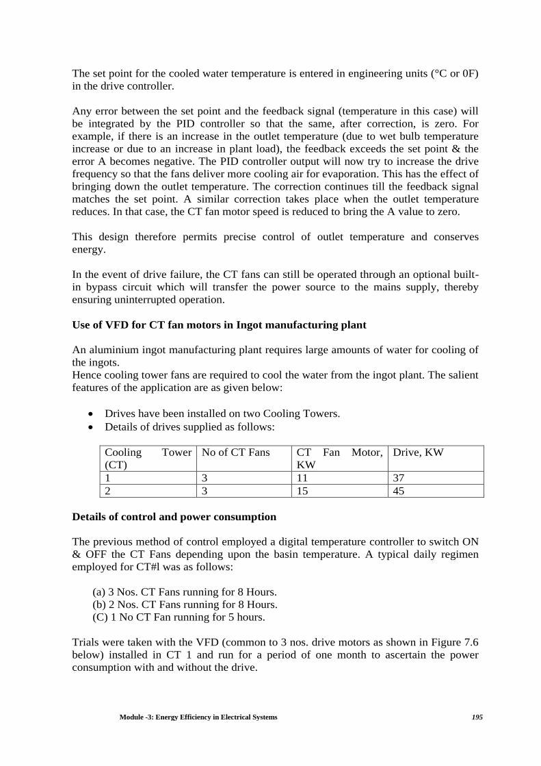
Module -3: Energy Efficiency in Electrical Systems 195
The set point for the cooled water temperature is entered in engineering units (°C or 0F)
in the drive controller.
Any error between the set point and the feedback signal (temperature in this case) will
be integrated by the PID controller so that the same, after correction, is zero. For
example, if there is an increase in the outlet temperature (due to wet bulb temperature
increase or due to an increase in plant load), the feedback exceeds the set point & the
error A becomes negative. The PID controller output will now try to increase the drive
frequency so that the fans deliver more cooling air for evaporation. This has the effect of
bringing down the outlet temperature. The correction continues till the feedback signal
matches the set point. A similar correction takes place when the outlet temperature
reduces. In that case, the CT fan motor speed is reduced to bring the A value to zero.
This design therefore permits precise control of outlet temperature and conserves
energy.
In the event of drive failure, the CT fans can still be operated through an optional built-
in bypass circuit which will transfer the power source to the mains supply, thereby
ensuring uninterrupted operation.
Use of VFD for CT fan motors in Ingot manufacturing plant
An aluminium ingot manufacturing plant requires large amounts of water for cooling of
the ingots.
Hence cooling tower fans are required to cool the water from the ingot plant. The salient
features of the application are as given below:
Drives have been installed on two Cooling Towers.
Details of drives supplied as follows:
Cooling Tower
(CT)
No of CT Fans CT Fan Motor,
KW
Drive, KW
1 3 11 37
2 3 15 45
Details of control and power consumption
The previous method of control employed a digital temperature controller to switch ON
& OFF the CT Fans depending upon the basin temperature. A typical daily regimen
employed for CT#l was as follows:
(a) 3 Nos. CT Fans running for 8 Hours.
(b) 2 Nos. CT Fans running for 8 Hours.
(C) 1 No CT Fan running for 5 hours.
Trials were taken with the VFD (common to 3 nos. drive motors as shown in Figure 7.6
below) installed in CT 1 and run for a period of one month to ascertain the power
consumption with and without the drive.

Module -3: Energy Efficiency in Electrical Systems 196
Note:
The applicable power supply voltage in this case would be 415V, 50Hz.
There is a bypass line which will enable the motors to operate from mains supply
in case of VFD failure.
Figure 7.6 Typical Power Schematic of VFD and CT fan motors
It was compared with the power consumed with manual operation (as described above)
on a daily basis. It yielded a significant result in terms of power saved daily.
Savings calculation with VFD operation:
Energy consumed daily with manual control (kWh) = 392
Energy consumed daily with VFD control (kWh) = 254
Energy saved on daily basis with VFD control (kWh) = 138
Energy saved on daily basis with VFD control (%) = 35.2
Unit energy cost (INR) = 5
Number of days of running of fans in a month = 26
Number of months in a year = 12
Annual savings due to VFD operation (INR) = 215280
Average price of drive panel (INR) = 250000
Payback period (Year) = 1.16
*Data for savings extrapolated for annual estimates
In practice, the power saved with VFD operation would also depend upon the wet bulb
temperature which would vary on a seasonal basis. In case of higher temperatures, the
VFD would be required to run at maximum speed during which period, the savings
would be negligible. Hence the average annual savings would reduce depending upon
the site environmental conditions. The quantum of savings can be optimized by having a
closed loop system as shown above which will track the outlet water temperature and
determine the drive motor speed accurately.

Module -3: Energy Efficiency in Electrical Systems 197
Example 7.2
The energy audit observations at a cooling tower (CT) in a process industry are given
below:
Cooling Water (CW) Flow: 3000 m3/hr
CW in Temperature: 4 1 deg. C
CW Out Temperature: 31 deg C
Wet Bulb Temperature: 24 deg. C
Find out Range, Approach, Effectiveness and cooling tower capacity in kcal per hour of
the CT?
Solution
Range = (Inlet -Outlet) Cooling Water Temperature deg. C
Range = (41 — 31) =10 deg. C
Approach = (Outlet Cooling Water - Air Wet Bulb) Temperature deg. C
Approach = (31 — 24) = 7 deg C
% CT Effectiveness = Range / (Range + Approach) x 100
% Effectiveness = 100 x [Range / (Approach + Range)]
10/ [10+7] x 100 = 58.8 %
Cooling capacity, kcal/hr = heat rejected = CW flow rate in kg per hour x (CW inlet hot
water temp. to CT, deg. C - CW outlet cold well temp, deg. C)
Cooling capacity = 3000X1000X (41 - 31) = 30,000,000 kCal per hour = 30 Million
kcal/hour.

Module -3: Energy Efficiency in Electrical Systems 198
Chapter 8: Lighting System
8.1 Introduction
Most natural light comes from the sun, including moon light. Its origin makes it
completely clean and it consumes no natural resources. But man-made sources generally
require consumption of resources, such as fossil fuels, to convert stored energy into light
energy.
Light is usually described as the type of electromagnetic radiation that has a wavelength
visible to the human eye, roughly 400 to 700 nanometers. Light exists as tiny “packets”
called photons and exhibits the properties of both particles and waves. Visible light, as
can be seen on the electromagnetic spectrum, as given in Figure 8.1, represents a narrow
band between ultraviolet light (UV) and infrared energy (heat). These light waves are
capable of exciting the eye’s retina, which results in a visual sensation called sight.
Therefore, seeing requires a functioning eye and visible light.
Figure 8.1: Visible Radiation
The lumen (1m) is the photometric equivalent of the Watt, weighted to match the eye
response of the “standard observer”. Yellowish—green light receives the greatest
weight because it stimulates the eye more than blue or red light of equal radiometric
power:
1 Watt = 683 lumens at 555 nm wavelength
The best eye sensitivity, as seen from Figure 8.2 is at 555 nm wavelength having
greenish yellow color with a luminous efficacy of 683 lm/Watt.

Module -3: Energy Efficiency in Electrical Systems 199
Figure 8.2: Relative Eye Sensitivity and Luminous Efficacy
Three primary considerations to ensure energy efficiency in lighting systems are:
i. Selection of the most efficient light source possible in order to minimize
electricity consumption and cost.
ii. Matching the proper lamp type to the intended work task or aesthetic application,
consistent with color, brightness control and other requirements.
iii. Establishing adequate light levels without compromising productivity improve
security and increase safety.
8.2 Basic Parameters and Terms in Lighting System
Luminous flux: The luminous flux describes the quantity of light emitted by a light
source. It is a measure of a lamp’s economic efficiency.
The most common measurement or unit of luminous flux is the lumen (lm).
The lumen rating of a lamp is a measure of the total light output of the lamp. Light
sources are labeled with an output rating in lumens.

Module -3: Energy Efficiency in Electrical Systems 200
Illuminance (E): is the quotient of the luminous flux incident on an element of the
surface at a point of surface containing the point, by the area of that element.
The lighting level produced by a lighting installation is usually qualified by the
illuminance produced on a specified plane. In most cases, this plane is the major plane
of the tasks carried out in the interior and is commonly called the working plane. The
illuminance provided by an installation affects both the performance of the tasks and the
appearance of the space. Lux (1X) is the metric unit of measure for illuminance of a
surface. One lux is equal to one lumen per square meter. Illuminance decreases by the
square of the distance (inverse square law).
The inverse square law defines the relationship between the illuminance from a point
source and distance. It states that the intensity of light per unit area is inversely
proportional to the square of the distance from the source (essentially the radius).
Where, E = Illuminance in lux (lm/mz), I = Luminous flux in lumen (1m) and
d = distance in m
An alternate form of this equation which is sometimes more convenient is:
Distance is measured from the test point to the first luminating surface - the filament of a
clear bulb or the glass envelope of a frosted bulb.
Example 8.1
The illuminance is 10 lm/m2 from a lamp at 1 meter distance. What will be the
illuminance at half the distance?
Solution:
Average maintained illuminance: is the average of illuminance (lux) levels measured
at various points in a defined area.
Circuit Watts: is the total power drawn by lamps and ballasts in a lighting circuit under
assessment.
Luminous Efficacy (lm/W): is the ratio of luminous flux emitted by a lamp to the
power consumed by the lamp. It is a reflection of efficiency of energy conversion from
electricity to light form. Unit: lumens per lamp Watt (lm/W).
Lamp Circuit Efficacy: is the amount of light (lumens) emitted by a lamp for each
Watt of power consumed by the lamp circuit, i.e. including control gear losses. This is a
more meaningful measure for those lamps that require control gear. Unit: lumens per
circuit Watt (lm/W).

Module -3: Energy Efficiency in Electrical Systems 201
Installed Load Efficacy: is the average maintained illuminance provided on a
horizontal working plane per circuit watt with general lighting of an interior. Unit: lux
per Watt per square metre (luX/W/m2).
Installed Power Density: The installed power density per 100 lux is the power needed
per square meter of floor area to achieve 100 lux of average maintained illuminance on a
horizontal working plane with general lighting of an interior. Unit: Watts per square
metre per 100 lux (W/m2/1001ux)
Color rendering index (CRI): is a measure of the effect of light on the perceived color
of objects. To determine the CR1 of a lamp, the color appearances of a set of standard
color chips are measured with special equipment under a reference light source with the
same correlated color temperature as the lamp being evaluated. If the lamp renders the
color of the chips identical to the reference light source, its CR1 is 100. If the color
rendering differs from the reference light source, the CR1 is less than 100. A low CR1
indicates that some colors may appear unnatural when illuminated by the lamp.
Luminaire: is a device that distributes filters or transforms the light emitted from one or
more lamps. The luminaire includes all the parts necessary for fixing and protecting the
lamps, except the lamps themselves. In some cases, luminaires also include the
necessary circuit auxiliaries, together with the means for connecting them to the electric
supply. The basic physical principles used in optical luminaire are reflection, absorption,
transmission and refraction.
Control gear: The gears used in the lighting equipment are as follows:
Ballast is a current limiting device, to counter negative resistance characteristics
of any discharge lamps. In case of fluorescent lamps, it aids the initial voltage
build-up, required for starting. In an electric circuit the ballast acts as a stabilizer.
Fluorescent lamp is basically an electric discharge lamp with two electrodes
separated inside a tube with no apparent connection between them. When
sufficient voltage is impressed on these electrodes, electrons are driven from one
electrode and attracted to the other. The current flow takes place through an
atmosphere of low-pressure mercury vapor.
Since the fluorescent lamps cannot produce light by direct connection to the
power source, they need an ancillary circuit and device to get started and remain
illuminated. The auxiliary circuit housed in a casing is known as ballast.
Ignitors are used for starting high intensity discharge lamps such as metal halide
and sodium vapor lamps. Ignitors generate a high voltage pulse or a series of
pulses to initiate the discharge.
8.3 Light Source and Lamp Types
Lamp is equipment, which produces light. Light is that part of the electromagnetic
spectrum that is perceived by our eyes. A number of light sources are available, each
with its own unique combination of operating characteristics viz., efficacy, color, lamp
life, and the percent of output that a lamp loses over its life.
Based on the construction and operating characteristics, the lamps can be categorized
into three groups: incandescent, fluorescent and high intensity discharge (HID) lamps.
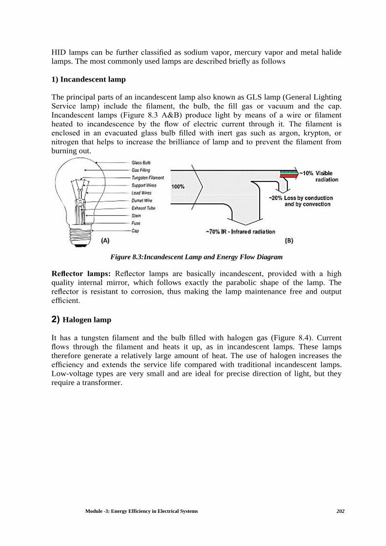
Module -3: Energy Efficiency in Electrical Systems 202
HID lamps can be further classified as sodium vapor, mercury vapor and metal halide
lamps. The most commonly used lamps are described briefly as follows
1) Incandescent lamp
The principal parts of an incandescent lamp also known as GLS lamp (General Lighting
Service lamp) include the filament, the bulb, the fill gas or vacuum and the cap.
Incandescent lamps (Figure 8.3 A&B) produce light by means of a wire or filament
heated to incandescence by the flow of electric current through it. The filament is
enclosed in an evacuated glass bulb filled with inert gas such as argon, krypton, or
nitrogen that helps to increase the brilliance of lamp and to prevent the filament from
burning out.
Figure 8.3:Incandescent Lamp and Energy Flow Diagram
Reflector lamps: Reflector lamps are basically incandescent, provided with a high
quality internal mirror, which follows exactly the parabolic shape of the lamp. The
reflector is resistant to corrosion, thus making the lamp maintenance free and output
efficient.
2) Halogen lamp
It has a tungsten filament and the bulb filled with halogen gas (Figure 8.4). Current
flows through the filament and heats it up, as in incandescent lamps. These lamps
therefore generate a relatively large amount of heat. The use of halogen increases the
efficiency and extends the service life compared with traditional incandescent lamps.
Low-voltage types are very small and are ideal for precise direction of light, but they
require a transformer.

Module -3: Energy Efficiency in Electrical Systems 203
Figure 8.4:Halogen Lamp
Tungsten atoms evaporate from the hot filament and move toward the cooler wall of the
bulb. Tungsten, oxygen and halogen atoms combine at the bulb-wall to form tungsten
oxyhalide molecules. The bulb-wall temperature keeps the tungsten oxyhalide
molecules in a vapor. The molecules move toward the hot filament where the higher
temperature breaks them apart. Tungsten atoms are re-deposited on the cooler regions of
the filament - not in the exact places from which they evaporated. Breaks usually occur
near the connections between the tungsten filament and its molybdenum lead-in wires
where the temperature drops sharply.
3) Fluorescent tube lamp (FTL)
It works by the fluorescence principle. A fluorescent lamp (Figure 8.5 A&B) is a glass
tube containing a small trace of a gas such as mercury vapor (for a white color), carbon
dioxide (for green), neon (for red color), etc., with a special fluorescent / phosphorescent
coating on the interior surface of the tube.
It contains two filaments, one at each end of the tube and when the electrical supply is
switched ON, the contacts of the starter open and the filaments glow to heat up the gas
contained inside the tube.
This action provides a voltage across its electrodes that set off an electric (gaseous
mercury) arc discharge in the tube. This generates invisible UV radiation that is high
enough to ionize the warmed-up gas inside the tube. This ionized gas also called as
“plasma”, excites the fluorescent coating so that it gives out visible light. Ballast is
needed to start and operate fluorescent lamps, because of the characteristics of a gaseous
arc. The luminous flux is highly dependent on the ambient temperature. Fluorescent
Lamps are about 3 to 5 times as efficient as standard incandescent lamps and can last
about 10 to 20 times longer.

Module -3: Energy Efficiency in Electrical Systems 204
The different types of fluorescent lamps and their reference are given below:
Linear tubes
T12 - 38 mm (1.5”diameter)
T8 - 25 mm (1”diameter)
T5 - 16mm (5/8”diameter)
T2 - 6 mm (l/4”diameter
Figure 8.5 (A): Fluorescent Tube Lamp
U-bent tubes
T12- 38 mm (1.5”diameter)
T8 - 25 mm (1” diameter)
Circular tubes
T9 - 38 mm (1.5”diameter)
T5 - 16 mm (5/8”diameter)
These four lamps vary in diameter (ranging from 1.5 inches that is 12/8 of an inch for
T12 to 0.625 or 5/8 of an inch in diameter for T5 lamps). Efficacy is another area that
distinguishes one from another. T5 & T8 lamps offer a 5-percent increase in efficacy
over 40-watt T12 lamps, and have become the most popular choice for new
installations.
4) Compact fluorescent lamp (CFL)
Compact Fluorescent lamps (Figure 8.6) are compact / miniature versions of the linear
or circular fluorescent lamps and operate in a very similar way. The luminous flux
depends on temperature. CFL’s use less power and have a longer rated life compared to
an incandescent lamp.
Figure 8.6: Compact Fluorescent Lamp
They are designed to replace an incandescent lamp and can fit into most existing light
fixtures formerly used for incandescent. CFL’s are available in screw type/ pin type
which fit into standard sockets, and gives off light that is similar to common fluorescent
lamps.

Module -3: Energy Efficiency in Electrical Systems 205
5) Sodium vapour lamp
Low pressure sodium vapour lamp
Although low pressure sodium vapour (LPSV) lamps (Figure 8.7) are similar to
fluorescent systems (because they are low pressure systems), they are commonly
included in the HID family. LPSV lamps are the most efficacious light sources, but they
produce the poorest quality light of all the lamp types. Being a monochromatic light
source, all colours appear black, white, or shades of gray under an LPSV source. LPSV
lamps are available in wattages ranging from 18-180.
Figure 8.7: LOW Pressure Sodium Vapour Lamp
LPSV lamp use has been generally limited to outdoor applications such as security or
street lighting and indoor, low-wattage applications where color quality is not important
(e. g. stairwells). However, because the color rendition is so poor, many municipalities
do not allow them for roadway lighting.
High pressure sodium vapour lamp
The high pressure sodium vapour (HPSV) lamp (Figure 8.8 A&B) is widely used for
outdoor and industrial applications as the light is yellowish. Its higher efficacy makes it
a better choice than metal halide for these applications, especially when good color
rendering is not a priority. HPSV lamps differ from mercury and metal-halide lamps in
that they do not contain starting electrodes; the ballast circuit includes a high-voltage
electronic starter. The arc tube is made of a ceramic material, which can withstand
temperatures up to 1300 °C. It is filled with xenon to help start the arc, as well as a
sodium-mercury gas mixture.
Figure 8.8 (A): High Pressure Sodium Vapour Lamp

Module -3: Energy Efficiency in Electrical Systems 206
Figure 8.8 (B): Energy Flow diagram of High Pressure Sodium Vapour Lamp
6) Mercury vapour lamp
In a mercury vapour lamp (Figure 8.9) electromagnetic radiation is created from
discharge within mercury vapour, but the regime is different than that found in the
normal fluorescent lamp. During operation, the pressure within the lamp is in the range
of 200 — 400 kPa (compared with only 1 Pa). It is not possible to achieve the mercury
vapour discharge in a cold lamp. For this reason, the lamp also includes argon, and the
initial arc is struck as an argon arc. The energy from this discharge vapourises the
mercury to get the main discharge going.
The mercury vapour lamp produces a much greater proportion of visible light than
fluorescent lamp and gives off a bluish white light. Phosphor coating can be given to
improve the colour rendering index.
Figure 8.9: Mercury Vapour Lamp and Energy Flow Diagram
7) Metal halide lamp:
Metal halide lamp (Figure 8.10 A&B) can be considered as a variant of high pressure
mercury vapour lamp (HPMV). In addition to mercury vapour and argon, this lamp
contains metal halide. The halides can be a mixture of rare earth halides, usually iodides
or a mixture of sodium and scandium iodide. The mercury vapour radiation is
augmented by that of the metals.
A highly compact electric arc is produced in a discharge tube. A starter is needed to
switch on the lamp. The use of ceramic discharge tubes further improves the lamp
properties. The halides act in a similar manner to the tungsten halogen cycle. As the
temperature increases there is disassociation of the halide compound releasing the metal
into the arc. The halides prevent the quartz wall getting attacked by the alkali metals. By

Module -3: Energy Efficiency in Electrical Systems 207
adding other metals to the mercury different spectrum can be emitted. Some lamps use a
third electrode for starting, but others, especially the smaller display lamps, require a
high voltage ignition pulse.
. Figure 8.10 (A): Metal Halide Lamp
Metal halide lamps have a significantly better colour rendering index than mercury
vapour and can be tailored by the choice of halides.
Figure 8.10 (B): Energy Flow Diagram of Metal Halide Lamp
8) Light emitting diode (LED) lamp
LEDs produce light in a very unique way; they produce light via a process called
electro-luminescence
(Figure 8.11), a process that starts by turning a semiconductor material into a
conducting material. A semiconductor with extra electrons is called N—type (negative)
material, since it has extra negatively- charged electrons. In N—type material, free
electrons can move from a negatively-charged area to a positively charged area. A
semiconductor with extra holes is called P-type (positive) material since it has extra
positively-charged gaps called holes. When excited with current the negative electron
leaves its atom and the P-type material’s positive attraction draws the free negative
electron into its hole, and the hole also moves toward the electron, so on and so forth.
As an electron travels to a hole, it carries energy, but in order to fit into the hole it must
release any extra energy, and when it does, the extra energy is released in the form of

Module -3: Energy Efficiency in Electrical Systems 208
light. When we maintain a steady flow of electrical current to the diode, it continues the
process of allowing electrons to flow from the negative charged material and fall into
the positive charged holes which maintains a steady stream of light out of the LED. The
actual LED is quite small in size, usually less than one square millimeter. Additional
optical components are added to shape and direct the light. LED’s are made of number
of inorganic semiconductor materials, many of which produce different colour of light.
Figure 8.11(A): Representation of LED light
The efficiency of LED’s has now risen sharply and is currently up to 200 lumens per
watt in the laboratory and in some products available on the market (although more
typical LED’s average output varies from 50 to 130 lumens per watt).
Because of the low power requirement for LED’s, using solar panels becomes more
practical and less expensive than running an electrical wire or using a generator. Hence
LED with battery backup for remote application is very economical. They do not radiate
light in 360 degrees as an incandescent does. The light will be bright wherever it is
focused.
Unlike incandescent and fluorescent lamps, LEDs are not inherently white light sources.
Instead, LEDs emit nearly monochromatic light, making them highly efficient for
colored light applications such as traffic lights and exit signs. However, to be used as a
general light source, white light is needed. White light can be achieved with LEDs in
three ways:
Phosphor conversion, in which a phosphor is used on or near the LED to convert the
colored light to white light; RGB systems, in which light from multiple monochromatic
LEDs (red, green, and blue) is mixed, resulting in white light; and a hybrid method,
which uses both phosphor-converted and monochromatic LEDs.

Module -3: Energy Efficiency in Electrical Systems 209
Figure 8.11 (B): Energy Flow diagram of LED Lamp
Advantages of LED technology is as follows Low power consumption, Directional light
output, High efficiency level, Long life: up to ~100,000 hour life if junction temperature
can be controlled, Instant switching on with no warm up time, High resistance to
switching cycles, High impact and vibration resistance, No UV or IR radiation, Color
control ability, allows dimming and Mercury free
LED’s also offer a number of promising environmental benefits, and they are often
viewed as the future of green lighting.
9) Induction lamp
Induction lamp is noted for ‘crisp white light output’. Uses a magnetic field to excite
gases — has no lamp parts to wear out. It consists of two main components: ballast and
a sealed gas-filled bulb. Light is produced via electromagnetic induction, without an
electrode or any electrical connection inside the bulb. Instead, high frequency
electromagnetic fields are induced from outside the sealed chamber. To produce light,
the ballast supplies the electric coils with high frequency electrical current. The ferrite
magnets on either side of the bulb then emit electromagnetic fields which excite
electrons within the bulb.

Module -3: Energy Efficiency in Electrical Systems 210
Figure 8.12: Representation of Induction Lamp
As the electrons accelerate inside the bulb, they collide with mercury atoms and produce
ultraviolet (UV) light radiation. The UV light then causes the special phosphor coating
inside the glass to react in a way that produces fluorescent light within the visible
spectrum. The light produced by Induction Lighting (Figure 8.12) achieves good Color
Rendering Index (CR1), with a Correlated Color Temperature.
Advantages of Induction lamps is as follows long burning hours, very less maintenance
required, instant on/ instant re—strike and energy efficient lighting.
Lamp features: The Table 8.1 shows the lamp features of different lamps.
Table 8.1 Luminous performance characteristic of commonly used Luminaries
Type of Lamp Lumens / Watt Color
Rendering
Index
Typical Application Typical life
(hours) Range Avg.
Incandescent 8-18 14 Excellent
(100)
Homes, restaurants,
general lighting,
emergency lighting
1000
Fluorescent
lamps
46-60 50 Good w.r.t.
coating
(67-77)
Offices, shops,
hospitals, homes
5000
Compact
fluorescent
lamps (CFL)
40-70 60 Very good
(85)
Hotels, shops, homes,
offices
8000-10000
High pressure
mercury
(HPMV)
44-57 50 Fair
(45)
General lighting in
factories, garages, car
parking, flood lighting
5000
Halogen
lamps
18-24 20 Excellent
(100)
Display, flood
lighting, stadium
exhibition grounds,
construction areas
2000-4000
High pressure
sodium
(HPSV) SON
67-121 90 Fair
(22)
General lighting in
factories, ware houses,
street lighting
6000-12000
Low pressure
sodium
(LPSV) SOX
101-175 150 Poor
(10)
Roadways, tunnels,
canals, street lighting
6000-12000

Module -3: Energy Efficiency in Electrical Systems 211
Metal halide
lamps
75-125 100 Good
(70)
Industrial bays, spot
lighting, flood
lighting, retail stores
8000
LED lamps 50-130 90 Very good
(80)
Office, industry,
outdoor, retail,
hospitality, etc
30,000-
60,000
Induction
Lamps
65-90 75 Very good
(80)
General lighting,
factories, warehouse,
street lighting, flood
lighting, etc
60,000-
1,00,000
8.4 Recommended Illuminance Levels for Various Tasks/Activities/Locations
Recommendations on Illuminance
Scale of
Illuminance:
The minimum illuminance for all non-working interiors, has been
mentioned as 20 Lux (as per IS 3646). A factor of approximately 1.5
represents the smallest significant difference in subjective effect of
illuminance. Therefore, the following scale of illuminances is
recommended.
20—30—50—75—100—150—200—300—500—750—1000—
1500—2000, ... Lux
Illuminance
ranges:
Because circumstances may be significantly different for different
interiors used for the same application or for different conditions for
the same kind of activity, a range of illuminances is recommended for
each type of interior or activity intended of a single value of
illuminance. Each range consists of three successive steps of the
recommended scale of illuminances. For working interiors the middle
value (R) of each range represents the recommended service
illuminance that would be used unless one or more of the factors
mentioned below apply.
The higher value (H) ofthe range should be used at exceptional cases where low
reflectance or contrasts are present in the task, errors are costly to rectify, visual work is
critical, accuracy or higher productivity is of great importance and the visual capacity of
the worker makes it necessary. Similarly, lower value (L) ofthe range may be used when
reflectances or contrasts are unusually high, speed and accuracy is not important and the
task is executed only occasionally.
Recommended Illumination
The following Table 8.2 gives the recommended illuminance range for different tasks
and activities for chemical sector. The values are related to the visual requirements ofthe
task, to user’s satisfaction, to practical experience and to the need for cost effective use
of energy (Source IS 3646 (Part I): 1992).

Module -3: Energy Efficiency in Electrical Systems 212
For recommended illumination in other sectors, reader may refer Illuminating Engineers
Society Recommendations Handbook.
Table 8.2 Recommended illuminance range for different tasks and activities for chemical sector
8.5 Methods of Calculating Illuminance - Lighting Design for Interiors
In order to design a luminaire layout that best meets the illuminance and uniformity
requirements of the job, two types of information are generally needed: average
illuminance level and illuminance level at a given point. Calculation ofilluminance at
specific points is often done to help the designer evaluate the lighting uniformity,
especially when using luminaires where maximum spacing recommendations are not
supplied, or where task lighting levels must be checked against ambient level.

Module -3: Energy Efficiency in Electrical Systems 213
If average levels are to be calculated, two methods can be applied:
1. For indoor lighting situations, the Zonal Cavity Method is used with data from a
coefficient of utilization table.
2. For outdoor lighting applications, a coefficient of utilization curve is provided,
the CU is read directly from the curve and the standard lumen formula is used.
Zonal Cavity Method for Indoor Lighting Calculations
The Zonal Cavity Method (sometimes called the Lumen Method) is the currently
accepted method for calculating average illuminance levels for indoor areas, unless the
light distribution is radically asymmetric. It is an accurate hand method for indoor
applications because it takes into consideration the effect that inter-reflectance has on
the level of illuminance.
Although it takes into account several variables, the basic premise that foot-candles are
equal to luminous flux over an area is not violated.
Figure 8.13 Typical Room Space
The basis of the Zonal Cavity Method is that a room is made up of three spaces or
cavities. The space between the ceiling and the fixtures, if they are suspended, is defined
as the “ceiling cavity”; the space between the work plane and the floor, the “floor
cavity”; and the space between the fixtures and the work plane, the “room cavity.”
Example 8.2
The step by step process of lighting design is illustrated below with the help of an
example. The Figure 8.13 shows the parameters of a typical space.
Step-1: Decide the required illuminance on work plane, the type of lamp and luminaire
A preliminary assessment must be made of the type of lighting required, a decision most
often made as a function of both aesthetics and economics. For normal office work,
illuminance of200 lux is desired.

Module -3: Energy Efficiency in Electrical Systems 214
For an air conditioned office space under consideration, we choose 36 W fluorescent
tube lights with twin tube fittings. The luminaire is porcelain-enameled suitable for the
above lamp. It is necessary to procure utilisation factor tables for this luminaire from the
manufacturer for further calculations.
Step-2: Collect the room data in the format given below
Typical reflectance values for using in L5, L6, L7 are:
Step-3: Calculate room index
Step 4: Calculate the utilisation factor
Utilisation factor is defined as the percent of rated bare-lamp lumens that exit the
luminaire and reach the work plane. It accounts for light directly from the luminaire as
well as light reflected off the room surfaces. Manufacturers will supply each luminaire
with its own CU table derived from a photometric test report.
Using tables available from manufacturers, it is possible to determine the utilisation
factor for different light fittings if the reflectance of both the walls and ceiling is known,
the room index has been determined and the type of luminaire is known. For twin tube
fixture, utilisation factor is 0.66, corresponding to room index of 2.5.

Module -3: Energy Efficiency in Electrical Systems 215
Step-5: To calculate the number of fittings required, the following formula is used
Where,
N = Number of Fittings
E = Lux Level Required on Working Plane
A = Area of Room (L x W)
F = Total Flux (Lumens) from all the Lamps in one Fitting
UF = Utilisation Factor from the Table for the Fitting to be Used
LLF = Light Loss Factor. This takes account of the depreciation
over time of lamp output and dirt accumulation on the fitting and walls of the building.
Light output = 3050 Lumens (Single Lamp)
LLF = Lamp lumen MF x Luminaire MF x Room surface MF
Where, MF = Maintenance Factor
Typical LLF values
So, 6 Numbers of Twin Tube Fixtures are required. Total number of 36 W lamp is 12.
Step 6: Space the luminaires to achieve desired uniformity
Every luminaire will have a recommended space to height ratio. In earlier design
methodologies, the uniformity ratio, which is the ratio of minimum illuminance to
average illuminance, was kept at 0.8 and suitable space to height ratio is specified to
achieve the uniformity. In modern designs incorporating energy efficiency and task
lighting the emerging concept is to provide a uniformity of 1/3 to 1/10 depending on the
tasks.

Module -3: Energy Efficiency in Electrical Systems 216
Figure 8.14: Arrangement of Fittings
Recommended value for the above luminaire is 1.5. If the actual ratio is more than the
recommended values, the uniformity of lighting will be less.
For a sample of arrangement of fittings, refer Figure 8.14. The luminaire closer to a wall
should be one half of spacing or less.
Luminaire Spacing
Spacing between luminaires = 10/3 = 3.33 m
Mounting height (L9-L8) = 2.0 m
Space to height ratio (SHR) = 3.33/2.0 = 1.66
This is close to the limits specified and hence accepted.
It is better to choose luminaires with larger SHR. This can reduce the number of fittings
and connected lighting load.
8.6 General Energy Saving Opportunities
Changing the light bulbs is not the only way to improve the use of lighting. Below are
some examples of many other options available:

Module -3: Energy Efficiency in Electrical Systems 217
a) Use natural day lighting
The utility of using natural day lighting instead of electric lighting during the day is well
known, but is being increasingly ignored especially in modern air-conditioned office
spaces and commercial establishments like hotels, shopping plazas etc. Industrial plants
generally use daylight in some fashion, but improperly designed day lighting systems
can result in complaints from personnel or supplementary use of electric lights during
daytime.
Some of the methods to incorporate day lighting are:
i. North lighting by use if single-pitched truss of the saw-tooth type is a common
industrial practice; this design is suitable for latitudes north of 23 i.e. in North
India. In South India, north lighting may not be appropriate unless diffusing
glasses are used to cut out the direct sunlight.
ii. Innovative designs are possible which eliminates the glare of daylight and blend
well with the interiors. Glass strips, running continuously across the breadth of
the roof at regular intervals, can provide good, uniform lighting on industrial
shop floors and storage bays.
iii. A good design incorporating sky lights with FRP material along with transparent
or translucent false ceiling can provide good glare-free lighting; the false ceiling
will also cut out the heat that comes with natural light.
iv. Use of atrium with FRP dome in the basic architecture can eliminate the use of
electric lights in passages of tall buildings.
v. Natural Light from windows should also be used. However, it should be well
designed to avoid glare. Light shelves can be used to provide natural light
without glare.
vi. Mounting Solar tube on the roof, with the help of advanced optics and special
duct work to direct sunlight deep into the buildings and spreading out over large
internal spaces providing heat and glare free day lighting for 8-10 hrs in a day

Module -3: Energy Efficiency in Electrical Systems 218
b) De-lamping to reduce excess lighting
De—lamping is an effective method to reduce lighting energy consumption. In some
industries, reducing the mounting height of lamps, providing efficient luminaires and
then de-lamping has ensured that the illuminance is hardly affected. De—lamping at
empty spaces where active work is not being performed is also a useful concept.
c) Task lighting
Task Lighting implies providing the required good illuminance only in the actual small
area where the task is being performed, while the general illuminance of the shop floor
or office is kept at a lower level; e. g. Machine mounted lamps or table lamps. Energy
saving takes place because good task lighting can be achieved with low wattage lamps.
The concept of task lighting if sensibly implemented, can reduce the no of general
lighting fixtures, reduce the wattage of lamps, save considerable energy and provide
better illuminance and also provide aesthetically pleasing ambience.
(d) Selection of high efficiency lamps and luminaries
The details of common types of lamps are summarised in Table 8.1 above. It is possible
to identify energy saving potential for lamps by replacing with more efficient types. The
following examples of lamp replacements are common. There may be some limitations
if colour rendering is an important factor. It may be noted that, in most cases, the
luminaires and the control gear would also have to be changed. The savings are large if
the lighting scheme is redesigned with higher efficacy lamps and luminaires.
e) Reduction of lighting feeder voltage
Figure 8.15 shows the effect of variation of voltage on light output and power
consumption for fluorescent tube lights. Similar variations are observed on other gas
discharge lamps like mercury vapour lamps, metal halide lamps and sodium vapour
lamps (Table 8.3 summarises the effects). Hence reduction in lighting feeder voltage can
save energy, provided the drop in light output is acceptable.
In many areas, night time grid voltages are higher than normal; hence reduction in
voltage can save energy and also provide the rated light output. Some manufacturers are
supplying reactors and transformers as standard products. A large number of industries
have used these devices and have reported saving to the tune of 5% to 15%. Industries
having a problem of higher night time voltage can get an additional benefit of reduced
premature lamp failures.

Module -3: Energy Efficiency in Electrical Systems 219
Figure 8.15 Effect of Voltage Variation on Fluorescent Tube light Parameters
Table 8.3 Variation in Light Output and Power Consumption
f) Electronic ballasts
Conventional electromagnetic ballasts (chokes) are used to provide higher voltage to
start the tube light and subsequently limit the current during normal operation.
Electronic ballasts are oscillators that convert the supply frequency to about 20,000 Hz
to 30,000 Hz. The basic functions of electronic ballast are:
To ignite the lamp
To stabilize the gas discharge
To supply the power to the lamp
The losses in electronic ballasts for tube lights are only about 1 Watt, in place of 10 to
15 Watts in standard electromagnetic chokes.
The additional advantage is that the efficacy of tube lights improves at higher
frequencies, resulting in additional savings if the ballast is optimised to provide the

Module -3: Energy Efficiency in Electrical Systems 220
same light output as with the conventional choke. Hence a saving of about 15 to 20
Watts per tube light can be achieved by use of electronic ballasts. With electronic
ballast, the starter is eliminated and the tube light lights up instantly without flickering.
g) Lighting controllers
Automatic control for switching off unnecessary lights can lead to good energy savings.
This includes dimmers, motion & occupancy sensors, photo sensors and timers.
h) Lighting maintenance
Maintenance is vital to lighting efficiency. Light levels decrease over time because of
aging lamps and dirt on fixtures, lamps and room surfaces. Together, these factors can
reduce total illumination by 50 percent or more, while lights continue drawing full
power. The basic maintenance includes cleaning of lamps and fixtures, cleaning and
repainting interiors, re-lamping etc.
8.7 Energy Efficient Lighting Controls
Occupancy Sensors
Occupancy-linked control can be achieved using infra-red, acoustic, ultrasonic or
microwave sensors, which detect either movement or noise in room spaces. These
sensors switch lighting on when occupancy is detected, and off again after a set time
period, when no occupancy movement detected. They are designed to override manual
switches and to prevent a situation where lighting is left on in unoccupied spaces. With
this type of system it is important to incorporate a built-in time delay, since occupants
often remain still or quiet for short periods and do not appreciate being plunged into
darkness if not constantly moving around.
Timed Based Control
Timed-turnoff switches are the least expensive type of automatic lighting control. In
some cases, their low cost and ease of installation makes it desirable to use them where
more efficient controls would be too expensive.
Types and features
The oldest and most common type of timed-turnoff switch is the “dial timer,” a spring-
wound mechanical timer that is set by twisting the knob to the desired time. Typical
units of this type are vulnerable to damage because the shaft is weak and the knob is not
securely attached to the shaft. Some spring- wound units make an annoying ticking
sound as they operate. Newer types of timed-turnoff switches are completely electronic
and silent. Electronic switches can be made much more rugged than the spring-wound
dial timer. These units typically have a spring-loaded toggle switch that turns on the
circuit for a preset time interval. Some electronic models provide a choice of time
intervals, which you select by adjusting a knob located behind the faceplate. Most
models allow occupants to turn off the lights manually. Some models allow occupants to
keep the lights on, overriding the timer. Timed- turnoff switches are available with a
wide range of time spans. The choice of time span is a compromise. Shorter time spans

Module -3: Energy Efficiency in Electrical Systems 221
waste less energy but increase the probability that the lights will turn off while someone
is in the space. Dial timers allow the occupant to set the time span, but this is not likely
to be done with a view toward optimising efficiency. For most applications, the best
choice is an electronic unit that allows the engineering staff to set a fixed time interval
behind the cover plate.
Daylight Linked Control
Photoelectric cells can be used either simply to switch lighting on and off, or for
dimming. They may be mounted either externally or internally. It is however important
to incorporate time delays into the control system to avoid repeated rapid switching
caused, for example, by fast moving clouds. By using an internally mounted
photoelectric dimming control system, it is possible to ensure that the sum of daylight
and electric lighting always reaches the design level by sensing the total light in the
controlled area and adjusting the output of the electric lighting accordingly. If daylight
alone is able to meet the design requirements, then the electric lighting can be turned
off. The energy saving potential of dimming control is greater than a simple
photoelectric switching system. Dimming control is also more likely to be acceptable to
room occupants.
Localized Switching
Localized switching should be used in applications which contain large spaces. Local
switches give individual occupants control over their visual environment and also
facilitate energy savings. By using localized switching it is possible to turn off artificial
lighting in specific areas, while still operating it in other areas where it is required, a
situation which is impossible if the lighting for an entire space is controlled from a
single switch.
Street Lighting Systems and Controls
Street lighting /Public lighting is one of the major electrical loads in municipal areas.
Number of street lights used in a Municipal area varies from 20000 — 50000 in
numbers depending on the kilometers of road illuminated within the municipal limits.
Typical electrical load of municipal lighting system varies 2MW to 7 MW. The type of
lamps used in Municipal area includes Fluorescent Tube light/ Mercury Vapor Lamps/
Sodium Vapor Lamps and Metal Halide Lamps. High Mast towers are also used at
strategic junctions in the Municipal area. LEDs are also used for traffic signaling
purpose in municipal areas.
Following controls are adopted to reduce energy consumption in street lighting system:
1. Timer control (Switch ON/OFF as per set timing)
2. Day light control(Based on illumination level)
3. Selective switching/alternate switching of street lights low traffic density areas
(after midnight).
4. Switching control based on lux levels. (after midnight)
5. Installations of Voltage controllers to be operated after midnight.
6. Installation of PLC controlled Lighting panels for effective control and
monitoring.

Module -3: Energy Efficiency in Electrical Systems 222
8.8 Standards and Labeling Programs for FTL Lamps
Considering the large number of fluorescent lamps (FTL) in usage, BEE has included
FTL under Standard and Labeling Programme (S&L). The S&L Programme covers 4
feet tubular fluorescent lamps (101mm) for wattages up to 40W. The S&L programme
includes 6500K colour temperature for halo-phosphates and 6500K, 4000K & 2700K
for tri-phosphate category. The star rating scheme for FTL is given in Table 8.4.
Table 8.4 Star Rating scheme for FTL (101 mm)
8.9 Lighting Case Study
Replacement of existing T12 Fluorescent lamps in street lighting system with LED
lamps
Existing: Fluorescent lamp (T12) fixture of40 numbers is connected to the entire
campus for security purpose. All the lights remain in operation for around 12 hours at
night (6 pm. to 6 am) every day throughout the year. All the light fixtures are equipped
with electromagnetic ballast which consumes around 12 to 14 watt of additional power
while in operation. Hence the power consumption of a single fluorescent light fixture
considering minimum ballast loss is 40+12=52 watts. The total light output of all the
fluorescent light fixtures is around 2400 lumen.
Proposed: It was proposed to replace existing lamps with high efficient LED lamps of
18 W with a luminous efficacy of around 120-140 lm/w. The total luminous output of
these lamps is around 2340 lumen.

Module -3: Energy Efficiency in Electrical Systems 223
Calculation

Module -3: Energy Efficiency in Electrical Systems 224
Chapter 9: Diesel / Natural Gas Power Generating System
9.1 Introduction
Reciprocating engines produce electricity using a combustible fuel and generator. In
addition to producing electricity, useful heat can be recovered from the exhaust gas
using a heat recovery steam generator (HRSG), or heat recovery system for hot water
(Figure 9.1). Heat can also be recovered from the lubricating oil cooler, the jacket water
cooler and/or the charge air cooler, and this recovered “waste” heat can be provided to a
heating load. In this case, the reciprocating engine power plant would be operating in a
Combined Heat & Power (CHP) or cogeneration mode. The energy performance of a
reciprocating engine is influenced by a number of factors such as the type of fuel, the
reciprocating engine power capacity, minimum capacity, availability, heat rate and heat
recovery efficiency.
Figure 9.1 Reciprocating Engine Cogeneration
Figure 9.1 Reciprocating Engine Cogeneration
There are two basic types of reciprocating engines - spark ignition and compression
ignition. Spark ignition engines use a spark (across a spark plug) to ignite a compressed
fuel-air mixture. Typical fuels for such engines are gasoline, natural gas and sewage and
landfill gas. Compression ignition engines compress air to a high pressure, heating the
air to the ignition temperature of the fuel, which then is injected. The high compression
ratio used for compression ignition engines results in a higher efficiency than is possible
with spark ignition engines. Diesel/heavy fuel oil is normally used in compression
ignition engines, although some are dual-fueled (natural gas is compressed with the
combustion air and diesel oil is injected at the top of the compression stroke to initiate
combustion).

Module -3: Energy Efficiency in Electrical Systems 225
Diesel Engine Cycle
Diesel engine is the prime mover, which drives an alternator to produce electrical
energy. In the Diesel engine, air is drawn into the cylinder and is compressed to a high
ratio (14:1 to 25:1). During this compression, the air is heated to a temperature of700—
90000 A metered quantity of diesel fuel is then injected into the cylinder, which ignites
spontaneously because of the high temperature. Hence, the diesel engine is also known
as compression ignition (CI) engine. DG set can be classified according to cycle type as:
two stroke and four stroke. However, the bulk of IC engines use the four stroke cycle.
Let us look at the principle of operation of the four-stroke diesel engine. The 4 stroke
operations in a diesel engine (Figure 9.2) are: induction stroke, compression stroke,
ignition and power stroke and exhaust stroke.
1st : Induction stroke - while the inlet valve is open, the descending piston draws in
fresh air.
2nd : Compression stroke - while the valves are closed, the air is compressed to a
pressure of up to 25 bar.
3rd : Ignition and power stroke - fuel is injected, while the valves are closed
(fuel injection actually starts at the end of the previous stroke), the fuel ignites
spontaneously and the piston is forced downwards by the combustion gases.
4th : Exhaust stroke - the exhaust valve is open and the rising piston discharges the
spent gases from the cylinder
Figure 9.2 Schematic Diagram of Four-Stroke Diesel Engine
Since power is developed during only one stroke, the single cylinder four-stroke engine
has a low degree of uniformity. Smoother running is obtained with multi cylinder
engines because the cranks are staggered in relation to one another on the crankshaft.
There are many variations of engine configuration, for example. 4 or 6 cylinder, in—
line, horizontally opposed, vee or radial configurations.
Gas Engines
A typical spark-ignited lean-burn engine is depicted in Figure 9.3. In this process, the
gas is mixed with air before the inlet valves. During the intake period, gas is also fed
into a small pre chamber, where the gas mixture is rich compared to the gas in the
cylinder. At the end of the compression phase the gas/air mixture in the pre chamber is

Module -3: Energy Efficiency in Electrical Systems 226
ignited by a spark plug. The flames from the nozzle of the pre chamber ignite the gas/air
mixture in the whole cylinder. Combustion is fast. After the working phase the cylinder
is emptied of exhaust and the process starts again. Reciprocating engines with modern
lean-bum technology reach close to 45% electrical efficiency.
Figure 9.3 Natural Gas Engine
DG Set as a System
A diesel generating set (Figure 9.4) should be considered as a system since its
successful operation depends on the well-matched performance of the components,
namely:
a) The diesel engine and its accessories.
b) The AC Generator.
c) The control systems and switchgear.
d) The foundation and power house civil works.
e) The connected load with its own components like heating, motor drives, lighting
etc.
It is necessary to select the components with highest efficiency and operate them at their
optimum efficiency levels to conserve energy in this system.

Module -3: Energy Efficiency in Electrical Systems 227
Figure 9.4 DG Set System
Selection Considerations
To make a decision on the type of engine, which is most suitable for a specific
application, several factors need to be considered. The two most important factors are:
power and speed of the engine. The power requirement is determined by the maximum
load. The engine power rating should be 10-20
% more than the power demand by the end use. This prevents overloading the machine
by absorbing extra load during starting of motors or switching of some types of lighting
systems or when wear and tear on the equipment pushes up its power consumption.
Speed is measured at the output shaft and given in revolutions per minute (RPM). An
engine will operate over a range of speeds, with diesel engines typically running at
lower speeds (1300 - 3000 RPM). There will be an optimum speed at which fuel
efficiency will be greatest. Engines should be run as closely as possible to their rated
speed to avoid poor efficiency and to prevent buildup of engine deposits due to
incomplete combustion - which will lead to higher maintenance and running costs. To
determine the speed requirement of an engine, one has to again look at the requirement
of the load. For some applications, the speed of the engine is not critical, but for other
applications such as a generator, it is important to get a good speed match. If a good
match can be obtained, direct coupling of engine and generator is possible; if not, then
some form of gearing will be necessary - a gearbox or belt system, which will add to the
cost and reduce the efficiency. There are various other factors that have to be
considered, when choosing an engine for a given application. These include the
following: cooling system, abnormal environmental conditions (dust, dirt, etc.), fuel
quality, speed governing (fixed or variable speed), poor maintenance, control system,
starting equipment, drive type, ambient temperature, altitude, humidity, etc. Suppliers or
manufacturers literature will specify the required information when purchasing an
engine. The efficiency of an engine depends on various factors, for example, load factor
(percentage of full load), engine size, and engine type.

Module -3: Energy Efficiency in Electrical Systems 228
Diesel Generator Captive Power Plants
Diesel engine power plants are most frequently used in small power (captive non-utility)
systems. The main reason for their extensive use is the higher efficiency of the diesel
engines compared with gas turbines and small steam turbines in the output range
considered. In applications requiring low captive power, without much requirement of
process steam, the ideal method of power generation would be by installing diesel
generator plants. The fuels burnt in diesel engines range from light distillates to residual
fuel oils. Most frequently used diesel engine sizes are between the range 4 to 15 MW.
For continuous operation, low speed diesel engine is more cost-effective than high
speed diesel engine.
Advantages of adopting Diesel Power Plants are:
Low installation cost
Short delivery periods and installation period
Higher efficiency (as high as 43 -45 %)
More efficient plant performance under part loads
Suitable for different type of fuels such as low sulphur heavy stock and heavy
fuel oil in case of large capacities.
Minimum cooling water requirements,
Adopted with air cooled heat exchanger in areas where water is not available
Short start up time
A brief comparison of different types of captive power plants (combined gas turbine and
steam turbine, conventional steam plant and diesel engine power plant) is given in Table
9.1. It can be seen from the Table that captive diesel plant wins over the other two in
terms of thermal efficiency, capital cost, space requirements, auxiliary power
consumption, plant load factor etc.
Table: Comparison of Different type of Captive Power Plant
Description Units Combined GT
& ST
Conventional
Steam Plant
Diesel Engine
Power Plant
Thermal
Efficiency
% 40 - 46 33 - 36 43 - 45
Initial
Investment of
Installed
Capacity
BDT/KW 8,500- 10,000
15,000-18,000 7,500 - 9,000
Space
requirement
125%
(approx.)
250%
(approx.)
100%
(approx.)
Construction
time
Months 24 - 30 42 - 48 12 - 15
Project period Months 30 - 36 52 - 60 12
Auxiliary
Power
Consumption
%
2 - 4 8 - 10 1.3 - 2.1
Plant Load
Factor
kWh/kW 6000 - 7000 5000 - 6000 7200 - 7500
Start Up Time
from Cold
Minutes About 10 120 - 180 15 - 20

Module -3: Energy Efficiency in Electrical Systems 229
Diesel Engine Power Plant Developments
The diesel engine developments have been steady and impressive. The specific fuel
consumption has come down from a value of 220 g/kWh in the 1970’s to a value of
around 160 g/kWh in present times. Slow speed diesel engine, with its flat fuel
consumption curve over a wide load range (50%-100%), compares very favorably over
other prime movers such as medium speed diesel engine, steam turbines and gas
turbines. With the arrival of modern, high efficiency turbochargers, it is possible to use
an exhaust gas driven turbine generator (Figure 9.5) to further increase the engine rated
output. The net result would be lower fuel consumption per kWh and further increase in
overall thermal efficiency.
Figure: Turbocharger
The diesel engine is able to burn the poorest quality fuel oils, unlike gas turbine, which
is able to do so with only costly fuel treatment equipment. Slow speed dual fuel engines
are now available using high-pressure gas injection, which gives the same thermal
efficiency and power output as a regular fuel oil engine.
9.2 Selection and Installation Factors
Sizing of a Genset:
a) If the DG set is required for 100% standby, then the entire connected load in HP /
kVA should be added. After finding out the diversity factor, the correct capacity
of a DG set can be found out.
Example 9.1
Connected Load = 650 kW
Diversity Factor = 0.54
(Demand / Connected load)
Max. Demand = 650 x 0.54 = 350 kW
% Loading = 70

Module -3: Energy Efficiency in Electrical Systems 230
Set rating = 350/0.7 = 500 kW
At 0.8 PF, rating = 625 kVA
b) For an existing installation, record the current, voltage and power factors (kWh /
kVAh) reading at the main bus-bar of the system at every half-an—hour interval
for a period of 2-3 days and during this period the factory should be having its
normal operations. The non-essential loads should be switched off to find the
realistic current taken for running essential equipment. This will give a fair
idea about the current taken from which the rating of the set can be calculated.
For existing installation:
kVA = √3 VI
kVA Rating = kVA/ Load Factor
where Load factor = Average kVA/ Maximum kVA
c) For a new installation, an approximate method of estimating the capacity of a
DG set is to add full load currents of all the proposed loads to be run in DG set.
Then, applying a diversity factor depending on the industry, process involved
and guidelines obtained from other similar units correct capacity can be arrived
at.
High Speed Engine or Slow/Medium Speed Engine
The normal accepted definition of high speed engine is 1500 rpm. The high speed sets
have been developed in India, whereas the slow speed engines of higher capacities are
often imported. The other features and comparison between high and medium / slow
speed engines are mentioned in Table 9.2 below:
Table 9.2 Comparison of High and Slow Speed Engine
Factor Slow speed engine High speed engine
Break mean effective
pressure -therefore wear
and tear and
consumption of spares
Low High
Weight to power ratio-
therefore sturdiness and
life
More Less
Space High Less
Type of use Continuous use Intermittent use
Period between
overhauls*
8000 hours 3200
Direct operating cost
(Include Lubricating
Oils, filters etc.
Less High
* Typical recommendations from manufacturers

Module -3: Energy Efficiency in Electrical Systems 231
Keeping the above factors and available capacities of DG set in mind, the cost of
economics for both the engines should be worked out before arriving at a decision.
Capacity Combinations
From the point of View of space, operation, maintenance and initial capital investment,
it is certainly economical to go in for one large DG set than two or more DG sets in
parallel.
Two or more DG sets running in parallel can be a advantage as only the short-fall in
power —depending upon the extent of power cut prevailing - needs to filled up. Also,
flexibility of operation is increased since one DG set can be stopped, while the other DG
set is generating at least 50% of the power requirement. Another advantage is that one
DG set can become 100% standby during lean and low power-cut periods.
Air Cooling Vs. Water Cooling
The general feeling has been that a water cooled DG set is better than an air cooled set,
as most users are worried about the overheating of engines during summer months. This
is to some extent is true and precautions have to be taken to ensure that the cooling
water temperature does not exceed the prescribed limits.
However, from performance and maintenance point of view, water and air cooled sets
are equally good except that proper care should be taken to ensure cross ventilation so
that as much cool air as possible is circulated through the radiator to keep its cooling
water temperature within limits. While, it may be possible to have air cooled engines in
the lower capacities, it will be necessary to go in for water cooled engines in larger
capacities to ensure that the engine does not get over-heated during summer months.
Safety Features
It is advisable to have short circuit, over load and earth fault protection on all the DG
sets. However, in case of smaller capacity DG sets, this may become uneconomical.
Hence, it is strongly recommended to install a circuit protection. Other safety equipment
like high temperature, low lube oil pressure cut-outs should be provided, so that in the
event of any of these abnormalities, the engine would stop and prevent damage. It is
also essential to provide reverse power relay when DG sets are to run in parallel to avoid
back feeding from one alternator to another.
Parallel Operation with Grid
Running the DG set in parallel with the mains from the supply undertakings can be done
in consultation with concerned electricity authorities. However, some supply
undertakings ask the consumer to give an undertaking that the DG set will not be run in
parallel with their supply. The reasons stated are that the grid is an infinite bus and
paralleling a small capacity DG set would involve operational risks despite normal
protections like reverse power relay, voltage and frequency relays.

Module -3: Energy Efficiency in Electrical Systems 232
Maximum Single Load on DG Set
The starting current of squirrel cage induction motors is as much as six times the rated
current for a few seconds with direct-on-line starters. In practice, it has been found that
the starting current value should not exceed 200 % of the full load capacity of the
alternator. The voltage and frequency throughout the motor starting interval recovers
and reaches rated values usually much before the motor has picked up full speed.
In general, the HP of the largest motor that can be started with direct on line starting is
about 50 % of the kVA rating of the generating set. On the other hand, the capacity of
the induction motor can be increased, if the type of starting is changed over to star delta
or to auto transformer starter, and with this starting the HP of the largest motor can be
up to 75 % of the kVA of Gen set.
Unbalanced Load Effects
It is always recommended to have the load as much balanced as possible, since
unbalanced loads cause heating of the alternator, which may result in unbalanced output
voltages. The maximum unbalanced load between phases should not exceed 10 % of the
capacity of the generating sets.
Neutral Earthing
The electricity rules clearly specify that two independent earths to the body and neutral
should be provided to give adequate protection to the equipment in case of an earth
fault, and also to drain away any leakage of potential from the equipment to the earth for
safe working.
Site Condition Effects on Performance Derating
Site condition with respect to altitude, intake temperature, cooling water temperature
and de-rate diesel engine output as shown in following Tables: 9.3 and 9.4.

Module -3: Energy Efficiency in Electrical Systems 233
Table 9.3 Altitude and Intake Temperature Corrections
Table 9.4 Derating due to Air Inter Cooler water Inlet
Water Temperature °C Flow % Derating %
25 100 0
30 125 3
35 166 5
40 166 8
9.3 Operational Factors
Load Pattern & DG Set Capacity
The average load can be easily assessed by logging the current drawn at the main
switchboard on an average day. The ‘over load’ has a different meaning when referred
to the D.G. set. Overloads, which appear insignificant and harmless on electricity board
supply, may become detrimental to a D.G.set, and hence overload on D.G. set should be
carefully analysed. Diesel engines are designed for 10% overload for 1 hour in every 12
hours of operation. The AC. generators are designed to meet 50% overload for 15
seconds as specified by standards. The D.G. set/s selection should be such that the
overloads are within the above specified limits. It would be ideal to connect steady loads
on DG set to ensure good performance. Alongside alternator loading, the engine loading
in terms of kW or BHP, needs to be maintained above 50%. Ideally, the engine and
alternator loading conditions are both to be achieved towards high efficiency.
Engine manufacturers offer curves indicating % Engine Loading vs fuel Consumption in
grams/BHP. Optimal engine loading corresponding to best operating point is desirable
for energy efficiency.
Alternators are sized for kVA rating with highest efficiency attainable at a loading of
around 70% and more. Manufacturer’s curves can be referred to for best efficiency point
and corresponding kW and kVA loading values.

Module -3: Energy Efficiency in Electrical Systems 234
Sequencing of Loads
The captive diesel generating set has certain limits in handling the transient loads. This
applies to both kW (as reflected on the engine) and kVA (as reflected on the generator).
In this context, the base load that exists before the application of transient load brings
down the transient load handling capability, and in case of AC. generators, it increases
the transient voltage dip. Hence, great care is required in sequencing the load on D.G.
set/s. It is advisable to start the load with highest transient kVA first followed by other
loads in the descending order of the starting kVA. This will lead to optimum sizing and
better utilization of transient load handling capacity of D.G. set.
Load Pattern
In many cases, the load will not be constant throughout the day. If there is substantial
variation in load, then consideration should be given for parallel operation of D.G. sets.
In such a situation, additional D.G. set(s) are to be switched on when load increases.
The typical case may be an establishment demanding substantially different powers in
first, second and third shifts. By parallel operation, D.G. sets can be run at optimum
operating points or near about, for optimum fuel consumption and additionally,
flexibility is built into the system. This scheme can be also be applied where loads can
be segregated as critical and non-critical loads to provide standby power to critical load
in the captive power system.
Load Characteristics
Some of the load characteristics influence efficient use of D.G. set. These characteristics
are entirely load dependent and cannot be controlled by the D.G. set. The extent of
detrimental influence of these characteristics can be reduced in several cases
Power Factor:
The load power factor is entirely dependent on the load. The AC. generator is designed
for the power factor of0.8 lag as specified by standards. Lower power factor demands
higher excitation currents and results in increased losses. Over sizing A.C. generators
for operation at lower power factors results in lower operating efficiency and higher
costs. The economical alternative is to provide power factor improvement capacitors.
Unbalanced Load:
Unbalanced loads on AC. generator leads to unbalanced set of voltages and additional
heating in AC. generator. When other connected loads like motor loads are fed with
unbalanced set of voltages additional losses occur in the motors as well. Hence, the load
on the AC. generators should be balanced as far as possible. Where single phase loads
are predominant, consideration should be given for procuring single phase A.C.
generator.
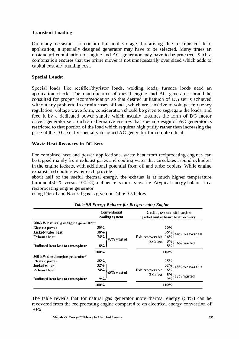
Module -3: Energy Efficiency in Electrical Systems 235
Transient Loading:
On many occasions to contain transient voltage dip arising due to transient load
application, a specially designed generator may have to be selected. Many times an
unstandard combination of engine and AC. generator may have to be procured. Such a
combination ensures that the prime mover is not unnecessarily over sized which adds to
capital cost and running cost.
Special Loads:
Special loads like rectifier/thyristor loads, welding loads, furnace loads need an
application check. The manufacturer of diesel engine and AC generator should be
consulted for proper recommendation so that desired utilization of DG set is achieved
without any problem. In certain cases of loads, which are sensitive to voltage, frequency
regulation, voltage wave form, consideration should be given to segregate the loads, and
feed it by a dedicated power supply which usually assumes the form of DG motor
driven generator set. Such an alternative ensures that special design of AC generator is
restricted to that portion of the load which requires high purity rather than increasing the
price of the D.G. set by specially designed AC generator for complete load.
Waste Heat Recovery in DG Sets
For combined heat and power applications, waste heat from reciprocating engines can
be tapped mainly from exhaust gases and cooling water that circulates around cylinders
in the engine jackets, with additional potential from oil and turbo coolers. While engine
exhaust and cooling water each provide
about half of the useful thermal energy, the exhaust is at much higher temperature
(around 450 °C versus 100 °C) and hence is more versatile. Atypical energy balance in a
reciprocating engine generator
using Diesel and Natural gas is given in Table 9.5 below.
Table 9.5 Energy Balance for Reciprocating Engine
The table reveals that for natural gas generator more thermal energy (54%) can be
recovered from the reciprocating engine compared to an electrical energy conversion of
30%.

Module -3: Energy Efficiency in Electrical Systems 236
It would be realistic to assess the Waste Heat Recovery (WHR) potential in relation to
quantity, temperature margin, in kcal/hr as:
Where, tg is the gas temperature after Turbocharger, (the criteria being that limiting exit
gas temperature cannot be less than 180°C, to avoid acid dew point corrosion), 0.25
being the specific heat of flue gases and kWh output being the actual average unit
generation from the set per hour. For a 1100 kVA set, at 800 kW loading, and with
480°C exhaust gas temperature, the waste heat potential works out to:
While the above method yields only the potential for heat recovery, the actual realizable
potential depends upon various factors and if applied judiciously, a well configured
waste heat recovery system can tremendously boost the economics of captive DG power
generation.
The factors affecting Waste Heat Recovery from flue Gases are:
a) DG Set loading, temperature of exhaust gases
b) Hours of operation and
c) Back pressure on the DG set
Consistent DG set loading (to over 60% of rating) would ensure a reasonable exit flue
gas quantity and temperature. Fluctuations and gross under loading of DG set results in
erratic flue gas quantity and temperature profile at entry to heat recovery unit, thereby
leading to possible cold end corrosion and other problems. Typical flue gas temperature
and flow pattern in a 5 MW DG set at various loads are given in Table 9.6
Table 9.6 Typical Flue gas Temperature and Flow pattern in a 5-MW DG Set at Various Load
100% Load 11.84 kg/sec 370°C
90% Load 10.80 kg/sec 350°C
70% Load 9.08 kg/sec 330°C
60% Load 7.50 kg/sec 325°C
If the normal load is 60%, the flue gas parameters for waste heat recovery unit would
be 325°Cinlet temperature, 180°C outlet temperature and 27180 kg/hour gas flow.
At 90% loading, however, values would be 350°C and 32,400 kgs/Hour, respectively.
* Number of hours of operation of the DG Set has an influence on the thermal
performance of waste heat Recovery unit. With continuous DG Set operations, cost
benefits are favorable.
* Back pressure in the gas path caused by additional pressure drop in waste heat
recovery unit is another key factor. Generally, the maximum back pressure allowed is
around 250-300 mmWC and the heat recovery unit should have a pressure drop lower

Module -3: Energy Efficiency in Electrical Systems 237
than that. Choice of convective waste heat recovery systems with adequate heat transfer
area are known to provide reliable
serv1ce.
The configuration of heat recovery system and the choice of steam parameters can be
judiciously selected with reference to the specific industry (site) requirements. Much
good work has taken place in Indian Industry regarding waste heat recovery and one
interesting configuration, deployed is installation of waste heat boiler in flue gas path
along with a vapour absorption chiller, to produce 8°C chilled water working on steam
from waste heat.
Trigeneration Technology
In order to further optimize fuel utilization Trigeneration systems are developed which
involves the simultaneous production of electricity, heat and cooling. The prime mover
used for power generation includes diesel engines/gas engines. The waste heat recovery
system in captive power generation units consists of waste heat recovery boiler for
generating steam and use of jacket cooling water for operating Vapor Absorption
Machines (VAM) to meet Air conditioning requirements.
9.4 Energy Performance Assessment of DG Sets
Routine energy efficiency assessment of DG sets on shop floor involves following
typical steps:
1) Ensure reliability of all instruments used for trial.
2) Collect technical literature, characteristics, and specifications of the plant.
3) Conduct a 2 hour trial on the DG set, ensuring a steady load, wherein the
following measurements are logged at 15 minutes intervals.
a) Fuel consumption (by dip level or by flow meter)
b) Amps, volts, PF, kW, kWh
c) Intake air temperature, Relative Humidity (RH)
d) Intake cooling water temperature
6) Cylinder-wise exhaust temperature (as an indication of engine loading)
f) Turbocharger RPM (as an indication of loading on engine)
g) Charge air pressure (as an indication of engine loading)
h) Cooling water temperature before and after charge air cooler (as an indication
of cooler performance)
i) Stack gas temperature before and after turbocharger (as an indication of
turbocharger performance)
4) The fuel oil/diesel analysis is referred to from an oil company data.
5) Analysis: The trial data is to be analysed with respect to:
a) Average alternator loading.
b) Average engine loading.
c) Percentage loading on alternator.
d) Percentage loading on engine.

Module -3: Energy Efficiency in Electrical Systems 238
e) Specific power generation kWh/liter.
f) Comments on Turbocharger performance based on RPM and gas
temperature difference.
g) Comments on charge air cooler performance.
h) Comments on load distribution among various cylinders (based on
exhaust temperature, the temperature to be i 5% of mean and high/low
values indicate disturbed condition).
i) Comments on housekeeping issues like drip leakages, insulation,
vibrations, etc.
A format as shown in the Table 9.7 is useful for monitoring the performance
Table 9.7 Typical format for DG set monitoring
9.5 Energy Saving Measures for DC Sets
a) Ensure steady load conditions on the DG set, and provide cold, dust free air at
intake (use of air washers for large sets, in case of dry, hot weather, can be
considered).

Module -3: Energy Efficiency in Electrical Systems 239
b) Improve air filtration.
c) Ensure fuel oil storage, handling and preparation as per manufacturer’s
guidelines/oil company data.
d) Consider fuel oil additives in case they benefit fuel oil properties for DG set
usage.
e) Calibrate fuel injection pumps frequently.
f) Ensure compliance with maintenance checklist.
g) Ensure steady load conditions, avoiding fluctuations, imbalance in phases,
harmonic loads.
h) In case of a base load operation, consider waste heat recovery system adoption
for steam generation or refrigeration chiller unit incorporation. Even the Jacket
Cooling Water is amenable for heat recovery, vapour absorption system
adoption.
i) In terms of fuel cost economy, consider partial use of biomass gas for generation.
Ensure tar removal from the gas for improving availability of the engine in the
long run.
j) Consider parallel operation among the DG sets for improved loading and fuel
economy thereof.
k) Carryout regular field trials to monitor DG set performance, and maintenance
planning as per requirements
Example 9.2
a) A 180 kVA, 0.80 PF rated DG set has diesel engine rating of 210 BHP. What is
the maximum power factor which can be maintained at fiill load on the alternator
without overloading the DG set? (Assume alternator losses and exciter power
requirement as 5.66 kW and there is no derating of DG set)
Solution
Engine rated Power = 210 X 0.746 = 156.66 kW
Rated power available for alternator = 15 6.66-5.66 = 151 kW
Maximum power factor possible = 151 /180 = 0.84
b) ADG set is operating at 600 kW load with 450°C exhaust gas temperature. The
DG set generates 8 kg of exhaust gas/ kWh generated. The specific heat of gas at
450°C is 0.25 kcal/ kg°C. A heat recovery boiler is installed after which the
exhaust temperature drops to 230°C. How much steam will be generated at 3 kg/
cm2 with enthalpy of 650.57 kcal/ kg. Assume boiler feed water temperature as
80°C.
Solution
Waste Heat Recovery = 600 kWh x 8 kg gas generated/ kWh output x 0.25 kcal/ kg °C x
(450°C-230 °C) =2,64,000 kcal/hr
Steam generation = 2,64,000 kcal/hr/ (650.57 — 80) = 462.7 kg/ hr.

Module -3: Energy Efficiency in Electrical Systems 240
Chapter 10: Energy Efficiency and Conservation in Buildings
10.1 Introduction
There are several different uses of energy in buildings. The major uses are for lighting,
heating, cooling, power delivery to equipment and appliances, and domestic water. The
amount that each contributes to the total energy use varies according to the climate, type
of building, number of working hours and time of year. Energy use for air-conditioning
has the largest share at a national level. In areas where severe winters occur, heating
load will be greater than cooling load in terms of the total energy use.
In some types of buildings in certain climatic zones, the lighting load might be greater
than either the heating or cooling loads.
Industrial and commercial buildings are dissimilar in terms of energy use, as industries
primarily use large quantities of energy for specialized processes whereas buildings use
the major amount of energy for human comfort. It is difficult to generalize energy use
by type of building because there are many variables that determine the energy use in a
particular building.
EE&C Potential in Residential Sector
If all the existing home appliances in residences are to be replaced by higher efficiency
products (as of today), huge energy reduction can be achieved. It is estimated that
EE&C potential is 28.8% of the total energy consumption in the residential sector.
Considering the fact that about 30% of national primary energy is consumed in the
residential sector, the potential economic impact of EE&C measures is massive: almost
8.6% of the total energy consumption in the country can be reduced.
EE&C Potential in Commercial Sector (Buildings)
Electricity is the main mode of energy in commercial buildings. In detail, nearly 50% of
the total energy is consumed by ACs and 10-30% by lighting systems. It is expected that
a simple replacement of ACs and lighting systems with high energy efficiency ones can
save about 50% of total electricity consumptions in the commercial sector. However it is
not easy to introduce EE&C measures for all the buildings. Thus as a realistic value,
EE&C potential for buildings was estimated about 10%.
10.2 Bangladesh National Building Code (BNBC):
In order to regulate tie technical details of building construction and to maintain the
standard of construction the Bangladesh National Building Code (BNBC) was first
published it 1993. Depletion of energy resources and environmental changes is a major
concern worldwide. Bangladesh is no exception to it. Keeping these aspects in mind,
changes and modifications have been suggested in BNBC 1993 for use of energy saving
appliances, non-conventional fuels etc. in buildings. The updated BNBC contains
chapters addressing the issues of energy conservation, rainwater harvesting and
distribution mechanisms in buildings. The updated BNBC has 10 parts with a total of 49
chapters. In Part 3, "General Building Requirements, Control and Regulation" a new
Chapter titled, "Energy Efficiency and Sustainability" has been included giving
minimum code requirements for achieving the efficiency.

Module -3: Energy Efficiency in Electrical Systems 241
To reduce energy consumption in building provisions for use of variable refrigeration
system in HVAC applications, Variable Voltage, Variable frequency drives in elevator
applications has been included in Chapter-2 "Air Conditioning, Heating and
Ventilation" of Part-8 "Building Services". Energy conservation in lighting using energy
saving lamps, Fluorescent lamps and GLS lamps has also been proposed in Chapter-1,
"Electrical and Electronics Engineering Services for Buildings" of the same part. To
augment water supply in Buildings, Chapter-8, "Rainwater Management" in Part-8
"Building Services" has been included in the Updated Code containing specific
guidelines for harvesting, storage and distribution of rainwater.
For more details please have a look of the Bangladesh National Building Code (BNBC).
The updated version of BNBC is proposed with addition of energy efficiency
requirement of buildings in near future BNBC will be the core program for promoting
EE&C in Buildings and contain the following requirement on building energy
efficiency:
a. Heat insulation and/or ventilation performance of building envelope
b. Energy efficiency of building equipment (HVAC, lighting, fans, hot water
supply, lift, escalator, renewable energy options)
c. Water efficiency and management and Sanitation
d. Roof gardening and vegetation
10.3 Building Energy & Environment Rating (BEER)
To ensure the energy efficiency in buildings, SREDA has developed the rating system
for buildings and act as the implementation and execution body for the Building Energy
& Environment Rating (BEER)
The objective to which the program aims to contribute is to:
Promote green and sustainable building practices on the supply and demand side
of Bangladesh’s construction sector;
Contribute to climate change mitigation by saving resources in the building
sector while enhancing economic prosperity and competitiveness, as well as
alleviating poverty by considering both green and social standards;
Establish a building energy efficiency and environmental rating systems serving
as a standard/reference for green building construction practices;
Enhance sustainable consumption in the building sector through a rating system,
providing consumer information and a distinctive grade for sustainable buildings;
Mobilize and capacitate key stakeholders to get involved in green building
design and construction.
Promote green equipment and construction materials, fixtures and make the
market ready.
Develop the capacity of architects and Engineers, Energy Managers & Energy
Auditors in Green Construction.
Provide access to soft and subsidize loan facilities for green building developer
and consumers.

Module -3: Energy Efficiency in Electrical Systems 242
Generally the Building should be Rated based on their typology. However, at the
beginning stage of the Building Energy and Environment Rating cover all types of
buildings by a single guideline. In next version, building typology (Existing Building,
New Construction, Interior space, Township, Industries etc.) specific rating guideline
will be developed.
The draft of BEER is available at SREDA website (www.sreda.gov.bd)
10.4 Energy Efficiency Measures in Buildings:
Air-Conditioning System:
Weather stripping of Windows and Doors
Minimize exfiltration of conditioned air and infiltration of external un-conditioned air
through leaky windows and doors by incorporating effective means of weather
stripping. Self-closing doors should also be provided where heavy traffic of people is
anticipated.
Temperature and Humidity Setting
Ensure human comfort by setting the temperature to between 23°C and 25°C and the
relative humidity between 55% and 65%.
Chilled Water Leaving Temperature
Ensure higher chiller energy efficiency by maintaining the chilled water leaving
temperature at or above 7° C. As a rule of thumb, the efficiency of a centrifugal chiller
increases by about 2% % for every 1° C rise in the chilled water leaving temperature.
Chilled Water Pipes and Air Ducts
Ensure that the insulation for the chilled water pipes and ducting system is maintained in
good condition.
This helps to prevent heat gain from the surroundings.
Chiller Condenser Tubes
Ensure that mechanical cleaning of the tubes is carried out at least once every six
months. Fouling in the condenser tubes in the form of slime and scales reduces the heat
transfer of the condenser tubes and thereby reducing the energy efficiency of the chiller.
Cooling Towers
Ensure that the cooling towers are clean to allow for maximum heat transfer so that the
temperature of the water returning to the condenser is less than or equal to the ambient
temperature.

Module -3: Energy Efficiency in Electrical Systems 243
Air-handling Unit Fan Speed
Install devices such as frequency converters to vary the fan speed. This will reduce the
energy consumption of the fan motor by as much as 15%.
Air Filter Condition
Maintain the filter in a clean condition. This will improve the heat transfer between air
and chilled water and correspondingly reduce the energy consumption.
Lighting System:
All lighting systems generate heat that needs to be dissipated. By designing energy
efficient lighting system that integrates day lighting and good controls, heat gains can be
reduced significantly. This can reduce the size of the HVAC system resulting in first-
cost savings.
Day lighting
Day lighting benefits go beyond energy savings and power reduction. Daylight spaces
have been shown to improve people’s ability to perform visual tasks, increase
productivity and reduce illness. Building fenestration should be designed to optimize
day lighting and reduce the need for electric lighting.
Orient the building to minimize building exposure to the east and west and maximize
glazing on the south and north exposures.
Daylight strategies do not save energy unless electric lights are turned off or dimmed
appropriately.
ECBC requires controls in day lit areas that are capable of reducing the light output
from luminaires by at least half.
Install dimmers to take advantage of day lighting and where cost-effective.
Replace rheostat dimmers with efficient electronic dimmers.
Combine time switching with day lighting using astronomical time clocks.
Control exterior lighting with photo controls where lighting can be turned off
after a fixed interval.
Switch off Lights When Not in Use
Provision of Separate Switches for Peripheral Lighting
A flexible lighting system, which made use of natural lighting for the peripherals of the
room, should be considered so that these peripheral lights can be switched off when not
needed.
Install High Efficiency Lighting System
Replace incandescent and other inefficient lamps with lamps with higher lighting
efficacy. For example, replacing incandescent bulbs with compact fluorescent lamps can
reduce electricity consumption by 75% without any reduction in illumination levels.

Module -3: Energy Efficiency in Electrical Systems 244
Fluorescent Tube Ballasts
The ballast losses of conventional ballast and electronic ballast are 12W and 2W
respectively. Hence, consider the use of electronic ballast for substantial energy savings
in the lighting system.
Lamp Fixtures or Luminaries
Optical lamp luminaries made of aluminum, silver or multiple dielectric coatings have
better light distribution characteristics. Use them to reduce electricity consumption by as
much as 50% without compromising on illumination levels.
Integration of Lighting System with Air-Conditioning System
In open plan offices, the air-conditioning and lighting systems can be combined in such
a way that the return air is extracted through the lighting luminaires. This measure
ensures that lesser heat will be directed from the lights into the room.
Cleaning of Lights and Fixtures
Clean the lights and fixtures regularly. For best results, dust at least four times a year.
Use Light Colors for Walls, Floors and Ceilings
The higher surface reflectance values of light colors will help to make the most of any
existing lighting system. Consider light colored furniture and room partitions to
optimize light reflectance. Avoid furniture colors and placement that will interfere with
light distribution. Keep ceilings and walls as bright as possible.
Deal with each activity area and each fixture individually
Eliminate excessive lighting by reducing the total lamp wattage in each activity area
Task Lighting
Lighting layout should use task lighting principle. Install focusing lamps or flexible
extensions wherever needed.
10.5 Building Water Pumping Systems
The pumps used in the buildings are for chilled water circulation, cooling water
circulation, domestic water, hot water and sewage water. The water requirement for
cooling, drinking and general purpose requirements in buildings are meat by the local
authorities and also from the independent bore wells.
The water received is stored and pumped to the overhead tanks provided on the building
terrace are hydro pneumatic system is used. Normally the pumps used in the building
are of centrifugal type with efficiencies of 60%. The following energy conservation
measures are adopted to reduce energy consumption in water pumping in buildings:

Module -3: Energy Efficiency in Electrical Systems 245
Installation of high efficiency pumps
Operation of pumps in parallel
Auto pump operation with low level/high level flow control systems.
Installation of variable frequency drive for chiller water and cooling water pumps
10.6 Uninterruptible power supply
An Uninterruptible Power Supply (UPS) is a device that has an alternate source of
energy, typically a battery backup that can provide power when the primary power
source is temporarily disabled. The switchover time must be small enough to not cause a
disruption in the operation of the loads (Figure 10.6).
The components of a UPS are converter (AC to DC), battery, inverter (DC to AC),
monitor and control hardware / software.
Figure 10.1 UPS Operation
There are two type of UPS architecture namely line interactive (OFF line) and ON line.
Simple OFF Line UPS systems, connect the load directly to the input AC line. Line
Interactive systems have also the ability to correct UPS output if AC input voltage
deviates beyond preset limits by means of an auto- transformer based Automatic
Voltage Regulator. In case of significant utility voltage deeps or outages these systems
transfer the UPS to battery operation.
Due to its direct connection to input AC power, OFF Line types, including Line
Interactive systems offer higher efficiency when compared to an Online UPS. But,
unstable grid environment, with frequent power interruptions or outages, might cause
these systems to suffer from frequent transfers to battery operation. Thus, exposing the
critical load to possible failures due to unsmooth or unsuccessful transfer, or to battery
failure, because of numerous battery discharges, which decrease drastically battery life
time.
An Online UPS system, frequently called Double conversion system, first converts the
AC input voltage to stabilized DC, which is then converted back to AC, to feed
continuously the critical load, with pure stabilized sinusoidal output, coming either from
the input line via AC/DC converter, or from batteries in case of power failure.
Energy efficiency of a UPS is the difference between the amount of energy that goes
into a UPS versus the amount of useful energy that comes out of the UPS and actually
powers loads (Figure 10.7). In all UPS systems some energy is lost as heat when it

Module -3: Energy Efficiency in Electrical Systems 246
passes through the internal components of the UPS (including transformers, rectifiers,
and inverters).
Figure 10.2 Energy Loss in UPS
Almost all UPS power 100% nonlinear loads +viz., computers, servers and electronic
equipment, though the manufacturers test their UPS often using linear loads. UPS
efficiency is often much higher when powering linear loads.
The second major factor to influence UPS efficiency is the power level at which the
efficiency is measured. Most UPSs typically have their best efficiency operating at 50%
to 100% load level. But in the real situation, most UPS systems operate at 25% to 60%
of their nominal load- not fully loaded.
To determine accurate efficiency, the UPS should demonstrate efficiency at loads
between 25—50%, where most UPS will likely to be operating.
10.7 Escalators and Elevators
The requirement of the maximum allowable electric power indicates ultimately the
energy performance of the equipment. The power for lift equipment is to be measured
when the lift is carrying its rated load and moving upward at its contract speed. For
escalators and passenger conveyors, since the rated load is usually defined as number of
person (not in kg weight), there is no theoretical rated load in kg for the equipment.
Thus the electric power is to be measured when the escalator/conveyor is carrying no
load and moving at its rated speed either in the upward or downward direction.
In escalators and elevators, the dominating factors that determine the energy
consumption are the efficiency of the motor, friction, the controller and the driving gear
box. The proportion of frictional loss of the machine can also become significant in the
power consumption in no load condition, as it is the fixed overhead to keep the
equipment running.
Factors That Affect Energy Consumption in Elevators and Escalator System
Energy is consumed by lift and escalator equipment mainly on the following categories:
Friction losses incurred while travelling.
Dynamic losses while starting and stopping.
Lifting (or lowering) work done, potential energy transfer.
Regeneration into the supply system.
The general approach to energy efficiency in lift and escalator equipment is merely to
minimize the friction losses and the dynamic losses of the system. There are many
factors that will affect these losses for elevator and escalator system:-

Module -3: Energy Efficiency in Electrical Systems 247
(A) Characteristic of the equipment
The type of motor, drive and control system of the machine, the internal decoration,
means to reduce friction in moving parts (e.g. guide shoes), type, speed and the pulley
system of the equipment.
(B) Characteristic of the premises
The population distribution, the type of the premises, the height of the premises and the
house keeping of the premises,
(C) The configuration of the lift/escalator system
The zoning of the lift system, the combination of lift and escalator equipment, the
strategies for vertical transportation and the required grade of service of the system.
General Principles to Achieve Energy Efficiency
In general the principles for achieving energy efficiency for lift/escalator installations
are as follows:
Specify energy efficiency equipment for the system.
Do not over design the system.
Suitable zoning arrangement.
Suitable control and energy management of lift equipment
Use lightweight materials for lift car decoration.
Good housekeeping.
10.8 Building Energy Management System (BEMS)
Energy management systems can vary considerably in complexity and degree of
sophistication. The simplest timing mechanism to switch systems ON and OFF at pre-
determined intervals on a routine basis could be considered as an energy management
system. These progresses to include additional features such as programmers,
thermostatic controls, motorized valves, zoning, and optimum start controllers and
compensated circuits.
The most complex of energy management systems have a computerized central
controller linked to numerous sensors and information sources. These could include the
basic internal and external range shown schematically in Figure 10.8, along with further
processed data to include: the time, the day of the week, time of year, percentage
occupancy of a building, meteorological data, system state feedback factors for plant
efficiency at any one time and energy gain data from the sun, lighting, machinery and
people.

Module -3: Energy Efficiency in Electrical Systems 248
Figure 10.3 Building Energy Management
A microprocessor is then the main feature of the control system. Data on temperature,
flow rates, pressures, etc., as appropriate, are collected from sensors 1n the system and
the treated spaces and stored in the memory of the processor. Provided that equations
defining the performance of the control elements, the items of plant and the behavioral
characteristics of the systems controlled have been developed and fed into the micro-
processor as algorithms, deviations from the desired performance can be dealt with by
calculation, the plant output being varied accordingly. Mathematical functions replace
control modes. For example, if room temperature rose in a space conditioned by a
constant volume reheat system, the correct position of the valve in the low temperature
hot water line feeding the heater battery could be calculated and corrected as necessary,
to bring the room temperature back to the set point as rapidly as possible, without any
offset. Data can be stored to establish trends and anticipation can be built into the
program so that excessive swings in controlled conditions may be prevented.
Furthermore, self-correction can be incorporated so that the control system learns from
experience and the best possible system performance is obtained. This implies that
commissioning inadequacies and possibly even design faults can be corrected but only
to a certain extent. Optimum results are only obtainable, and the cost of the installation
justified, from systems that have been properly designed, installed and commissioned.
Under such circumstances it is then feasible to extend the scope of microprocessor
control to include the management of all the building services with an economic use of
its thermal and electrical energy needs.
The functions of a building management system (BMS) or building energy management
system (BEMS) are monitoring and control of the services and functions of a building,
in a way that is economical and efficient in the use of energy. Furthermore, it may be
arranged that one system can control a group of buildings.

Module -3: Energy Efficiency in Electrical Systems 249
10.9 Energy performance Index: (EPI)
Energy Performance Index (EPI) in kWh / sq m/ year will be considered for rating the
building. Bandwidths for Energy Performance Index for different climatic zones have
been developed based on percentage air-conditioned space. For example a building in a
composite climatic zone like Dhaka and having air conditioned area greater than 50% of
their built up area, the bandwidths of EPI range between 190-90 kWh/sq m/year. Thus a
building would get a 5-Star rating if its EPI falls below 90 kWh/sq m/year and 1 Star if
it is between 165-190 kWh/ sq m/year.