Module 29 - Hypothesis Test for a Population Mean (1 of 5)

The following material comes from Concepts in Statistics written by the Open Learning Initiative (OLI) in conjunction with Carnegie Mellon and Stanford Universities (http://oli.cmu.edu)

Module 29 - Hypothesis Test for a Population Mean (1 of 5)

Introduction In Inference for Means, our focus is on inference when the variable is quantitative, so the parameters and statistics are means. In "Estimating a Population Mean," we learned how to use a sample mean to calculate a confidence interval. The confidence interval estimates a population mean. In "Hypothesis Test for a Population Mean," we learn to use a sample mean to test a hypothesis about a population mean.

We did hypothesis tests in earlier modules. In Inference for One Proportion, each claim involved a single population proportion. In Inference for Two Proportions, the claim was a statement about a treatment effect or a difference in population proportions. In "Hypothesis Test for a Population Mean," the claims are statements about a population mean. But we will see that the steps and the logic of the hypothesis test are the same. Before we get into the details, let’s practice identifying research questions and studies that involve a population mean.

EXAMPLE

Cell Phone Data

Cell phones and cell phone plans can be very expensive, so consumers must think carefully when choosing a cell phone and service. This decision is as much about choosing the right cellular company as it is about choosing the right phone. Many people use the data/Internet capabilities of a phone as much as, if not more than, they use voice capability. The data service of a cell company is therefore an important factor in this decision. In the following example, a student named Melanie from Los Angeles applies what she learned in her statistics class to help her make a decision about buying a data plan for her smartphone.

Melanie read an advertisement from the Cell Phone Giants (CPG, for short, and yes, we're using a fictitious company name) that she thinks is too good to be true. The CPG ad states that customers in Los Angeles get average data download speeds of 4 Mbps. With this speed, the ad claims, it takes, on average, only 12 seconds to download a typical 3-minute song from iTunes.

Only 12 seconds on average to download a 3-minute song from iTunes! Melanie has her doubts about this claim, so she gathers data to test it. She asks a friend who uses the CPG plan to download a song, and it takes 13 seconds to download a 3-minute song using the CPG network. Melanie decides to gather more evidence. She uses her friend’s phone and times the download of the same 3-minute song from various locations in Los Angeles. She gets a mean download time of 13.5 seconds for her sample of downloads.

What can Melanie conclude? Her sample has a mean download time that is greater than 12 seconds. Isn’t this evidence that the CPG claim is wrong? Why is a hypothesis test necessary? Isn’t the conclusion clear?


Let’s review the reason Melanie needs to do a hypothesis test before she can reach a conclusion.

Why should Melanie do a hypothesis test?

Melanie’s data (with a mean of 13.5 seconds) suggest that the average download time overall is greater than the 12 seconds claimed by the manufacturer. But wait. We know that samples will vary. If the CPG claim is correct, we don’t expect all samples to have a mean download time exactly equal to 12 seconds. There will be variability in the sample means. But if the overall average download time is 12 seconds, how much variability in sample means do we expect to see? We need to determine if the difference Melanie observed can be explained by chance.

We have to judge Melanie’s data against random samples that come from a population with a mean of 12. For this reason, we must do a simulation or use a mathematical model to examine the sampling distribution of sample means. Based on the sampling distribution, we ask, Is it likely that the samples will have mean download times that are greater than 13.5 seconds if the overall mean is 12 seconds?This probability (the P-value) determines whether Melanie’s data provides convincing evidence against the CPG claim.

Now let’s do the hypothesis test.

Step 1: Determine the hypotheses.

As always, hypotheses come from the research question. The null hypothesis is a hypothesis that the population mean equals a specific value. The alternative hypothesis reflects our claim. The alternative hypothesis says the population mean is “greater than” or “less than” or “not equal to” the value we assume is true in the null hypothesis.

Melanie’s hypotheses:

• H0: It takes 12 seconds on average to download Melanie’s song from iTunes with the CPG network in Los Angeles.

• Ha: It takes more than 12 seconds on average to download Melanie’s song from iTunes using the CPG network in Los Angeles.

We can write the hypotheses in terms of µ. When we do so, we should always define µ. Here μ = the average number of seconds it takes to download Melanie’s song on the CPG network in Los Angeles.

• H0: μ = 12 • Ha: μ > 12

Step 2: Collect the data.

To conduct a hypothesis test, Melanie knows she has to use a t-model of the sampling distribution. She thinks ahead to the conditions required, which helps her collect a useful sample.


Recall the conditions for use of a t-model.

• There is no reason to think the download times are normally distributed (they might be, but this isn't something Melanie could know for sure). So the sample has to be large (more than 30).

• The sample has to be random. Melanie decides to use one phone but randomly selects days, times, and locations in Los Angeles.

Melanie collects a random sample of 45 downloads by using her friend’s phone to download her song from iTunes according to the randomly selected days, times, and locations.

Melanie’s sample of size 45 downloads has an average download time of 13.5 seconds. The standard deviation for the sample is 3.2 seconds. Now Melanie needs to determine how unlikely this data is if CPG’s claim is actually true.

Step 3: Assess the evidence.

Assuming the average download time for Melanie’s song is really 12 seconds, what is the probability that 45 random downloads of this song will have a mean of 13.5 seconds or more?

This is a question about sampling variability. Melanie must determine the standard error. She

knows the standard error of random sample means is . Since she has no way of knowing the population standard deviation, σ, Melanie uses the sample standard deviation, s = 3.2, as an approximation. Therefore, Melanie approximates the standard error of all sample means (n = 45) to be

The sample mean for Melanie’s random sample is approximately 3.14 standard errors above the overall mean of 12. We know from previous experience that a sample mean this far above µ is very unlikely. With a t-score this large, the P-value is very small. We use an applet of the t-model for 44 degrees of freedom to verify this.


We want the probability that the sample mean is greater than 13.5. This corresponds to the probability that T is greater than 3.14. The P-value is 0.0015.

Step 4: State a conclusion.

Here the logic is the same as for other hypothesis tests. We use the P-value to make a decision. The P-value helps us determine if the difference we see between the data and the hypothesized value of µ is statistically significant or due to chance. One of two outcomes can occur:

• One possibility is that results similar to the actual sample are extremely unlikely. This means the data does not fit with results from random samples selected from the population described by the null hypothesis. In this case, it is unlikely that the data came from this population. The probability as measured by the P-value is small, so we view this as strong evidence against the null hypothesis. We reject the null hypothesis in favor of the alternative hypothesis.

• The other possibility is that results similar to the actual sample are fairly likely (not unusual). This means the data fits with typical results from random samples selected from the population described by the null hypothesis. The probability as measured by the P-value is large. In this case, we do not have evidence against the null hypothesis, so we cannot reject it in favor of the alternative hypothesis.

Melanie’s data is very unlikely if µ = 12. The probability is essentially zero (P-value = 0.0015). This means we will rarely see sample means greater than 13.5 if µ = 12. So we reject the null and accept the alternative hypothesis. In other words, this sample provides strong evidence that CPG has overstated the speed of its data download capability.


Comment In the previous example, Melanie did not state a significance level for her test. If she had, the logic is the same as we used for hypothesis tests in Modules 8 and 9. To come to a conclusion about H0, we compare the P-value to the significance level α.

• If P ≤ α, we reject H0. We conclude there is significant evidence in favor of Ha. • If P > α, we fail to reject H0. We conclude the sample does not provide significant

evidence in favor of Ha.

Content by the Open Learning Initiative and licensed under CC BY.


More on Checking Conditions for a T-Test In practice, you will often see the use of a t-test with small samples. Technically, we can use the t-test with small samples only if we know the variable has a normal distribution in the population. But this is hard to verify. In addition, no variable has a perfect normal distribution. So what does the requirement that the “variable be normally distributed in the population” really mean?

We call a confidence interval or a hypothesis test robust if the confidence level or P-value does not change very much when the conditions for use of the procedure are not met.

T-procedures are robust when the variable is not normally distributed in the population, as long as the distribution is not heavily skewed. But how can we determine if the distribution of the variable in the population is heavily skewed? In this introductory course, we examine the distribution of the variable in the sample and make an educated guess about what is going on in the population.

Now we investigate this question: Can we tell from a sample whether the variable is normally distributed in the population?

https://oli.cmu.edu/

https://creativecommons.org/licenses/by/3.0/


EXAMPLE

Variable Skewed in the Population

Let’s start with a skewed distribution in the population. Can we tell that this distribution is not normal by looking at random samples?

The following figure shows the monthly payment on first home mortgages for 5,000 people, as reported in the 2000 U.S. Census. Think of this as data from the population of a small town. From this population, we randomly selected 20 people. We did this three times. Notice that for each random sample, the shape of the distribution of the monthly payments in the sample is skewed to the right, just like the distribution in the population. In 2 of the 3 samples, we also see outliers, just as we see in the population. So by looking at the sample, we can get a pretty good sense that the variable is not normally distributed in the population.

In this example, the sample size is less than 30. We can use the t-test only if the variable is normally distributed in the population. The shape of the distribution in any one of these samples suggests that the variable has a skewed distribution in the population, so we would not conduct a t-test with any of these samples.


EXAMPLE

Variable Normal in the Population

Now we look at a variable that has an approximately normal distribution in the population. Can we tell that this distribution is approximately normal by looking at random samples?

The following graphs show the heights (in centimeters) of 5,000 women. Think of this as data from the population of a small town. From this population, we randomly selected 20 women. We did this three times. Notice that for each random sample, the shape of the distribution of the heights in the sample is not skewed, and there are no outliers. By looking at the sample, we can get a pretty good sense that the variable is not skewed in the population, which suggests that the variable may be somewhat normally distributed in the population.

In this example, the sample size is less than 30. We can only use the t-test if the variable is normally distributed in the population. The shape of the distribution in any one of these samples indicates that the variable does not have a skewed distribution in the population, suggesting that the distribution in the population is somewhat normal. Since the t-procedures are robust, we would conduct a t-test with any of these samples.

What’s the Main Point? We previously stated the conditions for use of the t-procedures as follows:

(1) If the variable is normally distributed in the population, you can always use the t-procedures.

(2) If the variable is not normally distributed in the population (or you can’t determine this factor), the sample size must be greater than 30 for safe use of the t-procedures.

We are now loosening these conditions somewhat because the t-procedures are robust.


(3) If the sample is small (n ≤ 30), plot the data. If the distribution in the sample is not heavily skewed and does not have outliers, then we assume the variable is somewhat normally distributed in the population, so we use t-procedures.

Comment If we use a t-procedure for a small sample (n ≤ 30), it is good practice to include a disclaimer with the conclusion. We might say something like, “On the basis of the sample, we are assuming that the variable is distributed without strong skew or extreme outliers in the population. The conclusion from this test is valid only if this assumption is true.”

Comment Recall that the sample mean and standard deviation are not resistant to outliers. An outlier in the data can make the mean and standard deviation poor measures of center and spread. So why can we use data from large samples even if the data has an outlier? Well, if the sample is large enough, the distribution of sample means will still be approximately normal. And the t-model will be a good fit when we estimate the standard error of the sample means using the sample standard deviation. This is the important point. The P-value and confidence level come from a model of the sampling distribution, not from a model of the population’s distribution.

Summary in a Diagram




Another common use of the t-test for a population mean is in “before and after” situations. In this situation, we have two quantitative measurements from a single sample of individuals. This is an example of a matched-pairs design.

EXAMPLE

Drinking and Driving

The Centers for Disease Control and Prevention (CDC) website cites studies from the National Highway Traffic Safety Administration to support this statement: “Alcohol use slows reaction time and impairs judgment and coordination, which are all skills needed to drive a car safely. The more alcohol consumed, the greater the impairment.” All states in the United States have




adopted a blood alcohol concentration of 0.08% (80 mg/dL) as the legal limit for operating a motor vehicle. The CDC website continues, “Note: Legal limits do not define a level below which it is safe to operate a vehicle or engage in some other activity. Impairment due to alcohol use begins to occur at levels well below the legal limit.”

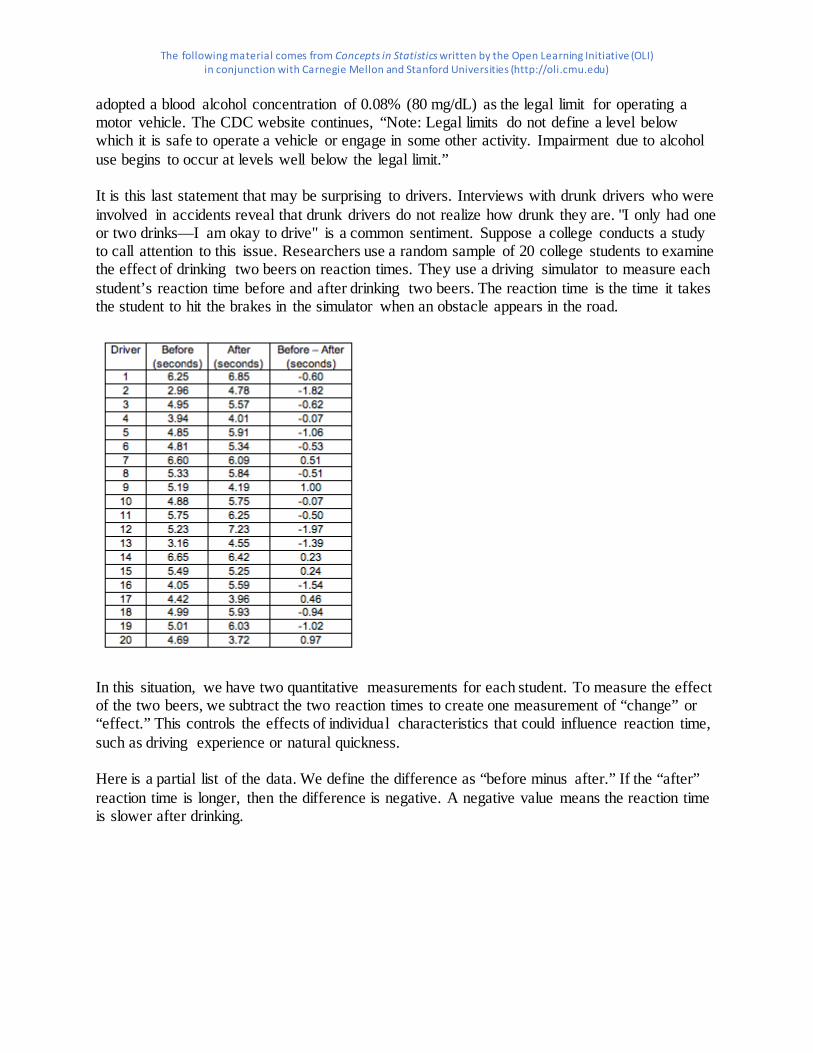
It is this last statement that may be surprising to drivers. Interviews with drunk drivers who were involved in accidents reveal that drunk drivers do not realize how drunk they are. "I only had one or two drinks—I am okay to drive" is a common sentiment. Suppose a college conducts a study to call attention to this issue. Researchers use a random sample of 20 college students to examine the effect of drinking two beers on reaction times. They use a driving simulator to measure each student’s reaction time before and after drinking two beers. The reaction time is the time it takes the student to hit the brakes in the simulator when an obstacle appears in the road.

In this situation, we have two quantitative measurements for each student. To measure the effect of the two beers, we subtract the two reaction times to create one measurement of “change” or “effect.” This controls the effects of individual characteristics that could influence reaction time, such as driving experience or natural quickness.

Here is a partial list of the data. We define the difference as “before minus after.” If the “after” reaction time is longer, then the difference is negative. A negative value means the reaction time is slower after drinking.


Note: It is common to define the difference in measurements as “before minus after.” But we could also define the difference the other way around as “after minus before.” In this definition, if the “after” reaction time is longer, then the difference is positive, so a slower reaction time after drinking corresponds to a positive value. This makes less intuitive sense to us. We want “negative” to mean “drinking has a negative effect,” so we used the other definition, “before minus after.”


The null hypothesis is a claim of “no change” or “no effect.” The alternative hypothesis reflects the claim.

• H0: Drinking two beers has no effect on reaction time. • Ha: Drinking two beers slows reaction time.

If drinking two beers has no effect on reaction time, then the mean of the differences in reaction times (before minus after) will be zero. If drinking two beers slows reaction time, then the mean of the differences in reaction times (before minus after) will be negative. So we can rewrite our hypotheses as follows.

• H0: μ = 0 • Ha: μ < 0

where µ is the mean of the difference in reaction time (before minus after) for all students at this college after drinking two beers.

Suppose researchers set a significance level of 5%.

Note: if we defined the difference in reverse order as “after minus before,” then a positive difference corresponds to a slower reaction time. This changes the alternative hypothesis to Ha: µ > 0. This will not effect the P-value or our conclusion. You just have to make sure the alternative hypothesis says what you want it to say given the way you define the difference.

Note: In some textbooks and other statistical materials, you will see the “mean of the difference” written as μd.



Here is the (made-up) data from this sample of 20 college students. The mean of the differences (before minus after) is approximately −0.46 seconds, and the standard deviation is approximately 0.87 seconds.


Check the Criteria for Use of a T-Model

The sample size is only 20, and we do not know if these differences would be normally distributed in general when comparing these two treatments in the population of all college students. We therefore do not meet the conditions for use of a t-model. Some researchers would stop here and not complete the hypothesis test. Others would check the shape of the distribution of differences in the sample. If the sample is approximately normal (or at least not heavily skewed), then they view this as a hopeful indication that the distribution in the population will also be approximately normal, and they continue with the hypothesis test, adding a disclaimer to the conclusion.

Here is a histogram of the differences in the sample.


The data is not heavily skewed, so we are willing to proceed with the t-test.

Compute the Test Statistic

Find the P-value.

We use the applet with the t-model for 19 degrees of freedom (df = n − 1 = 20 − 1 = 19). The P-value is approximately 0.015.


Step 4: State a conclusion.

The P-value (0.015) is less than the significance level (0.05), so we reject the null and accept the alternative hypothesis that µ < 0.

This study suggests that reactions times when driving are significantly slower after drinking two beers for students at this college. (P = 0.015).

It is good practice to include a disclaimer with this conclusion because the sample is small. We might add the following to our conclusion if we were publicly presenting these results: “The sample was too small to formally met the requirements for a t-test. On the basis of the data, we are assuming that the difference in reaction times would be normally distributed in general when comparing these two treatments in the population of all college students. The conclusion from this test is valid only if this assumption is true.”

Comment From this study, can we generalize to a larger population of “all college students” or “all drivers”? Technically, such a generalization requires that the sample be randomly selected from the more general population. Is this type of random sampling done in practice? Not always. The matched pairs design controls for individual differences that would otherwise confound such a generalization. This is one of the reasons that researchers run hypothesis tests with data gathered by groups like the National Highway Traffic Safety Administration, even when participants are not randomly selected. But ideally we should select samples randomly from the population of interest.

Can we make a cause-and-effect conclusion from this study?

We should be cautious about a cause-and-effect conclusion here because there is no random assignment. We take measurements from every student in both the treatment and the control setting without randomizing the treatment order. Every participant did the driving test sober, then drank two beers and did the driving test again. Technically, we need a more sophisticated study design that uses random assignment in order to make cause-and-effect conclusions. For example, we could randomly assign the treatment order for each student by flipping a coin, assigning some students do the first driving test while sober and others do the first driving test after drinking two beers. Then everyone comes back on another day to complete the part of the experiment that he or she had not done.






This page contains four opportunities for practicing the hypothesis test for a population mean from start to finish. The last two activities guide you through this hypothesis test using data and your statistical software package.

How Much Are College Students Sleeping?

(not including naps in class!)

Scenario: Americans average 6.9 hours of sleep on weeknights, according to a report released in 2011 by the National Sleep Foundation. A student in a statistics class at Los Medanos College wondered if the average amount of sleep on weeknights is different for LMC students. She collected data from a survey of 43 randomly selected students at LMC. Respondents averaged 7.12 hours of sleep a night with a standard deviation of 1.45 hours.

Texting and Concentration Scenario: An instructor at Los Medanos College conducted an experiment with her statistics class to study the effect of texting on concentration. She created two audio clips in which she read two different lists of words. The treatment required students to send a short text message to a friend while listening to one of the audio clips. In the control setting, students simply listened to one of the audio clips. Everyone wore earphones and listened to the audio clips in the same order. But a coin flip determined who was and was not texting each time. After each listening session, students had 2 minutes to write down all the words they could remember. Twenty three students participated in the experiment.




We finish our discussion of the hypothesis test for a population mean with a review of the meaning of the P-value, along with a review of type I and type II errors.

Review of the Meaning of the P-value At this point, we assume you know how to use a P-value to make a decision in a hypothesis test. The logic is always the same. If we pick a level of significance (α), then we compare the P-value to α.

• If the P-value ≤ α, reject the null hypothesis. The data supports the alternative hypothesis.

• If the P-value > α, do not reject the null hypothesis. The data is not strong enough to support the alternative hypothesis.

In fact, we find that we treat these as “rules” and apply them without thinking about what the P-value means. So let’s pause here and review the meaning of the P-value, since it is the connection between probability and decision-making in inference.

EXAMPLE

Birth Weights in a Town

Let’s return to the familiar context of birth weights for babies in a town. Suppose that babies in the town had a mean birth weight of 3,500 grams in 2010. This year, a random sample of 50 babies has a mean weight of about 3,400 grams with a standard deviation of about 500 grams. Here is the distribution of birth weights in the sample.

Obviously, this sample weighs less on average than the population of babies in the town in 2010. A decrease in the town’s mean birth weight could indicate a decline in overall health of the town. But does this sample give strong evidence that the town’s mean birth weight is less than 3,500 grams this year?




We now know how to answer this question with a hypothesis test. Let’s use a significance level of 5%.

Let μ = mean birth weight in the town this year. The null hypothesis says there is “no change from 2010.”

• H0: μ < 3,500 • Ha: μ = 3,500

Since the sample is large, we can conduct the T-test (without worrying about the shape of the distribution of birth weights for individual babies.)

Statistical software tells us the P-value is 0.082 = 8.2%. Since the P-value is greater than 0.05, we fail to reject the null hypothesis.

Our conclusion: This sample does not suggest that the mean birth weight this year is less than 3,500 grams (P-value = 0.082). The sample from this year has a mean of 3,400 grams, which is 100 grams lower than the mean in 2010. But this difference is not statistically significant. It can be explained by the chance fluctuation we expect to see in random sampling.

What Does the P-Value of 0.082 Tell Us? A simulation can help us understand the P-value. In a simulation, we assume that the population mean is 3,500 grams. This is the null hypothesis. We assume the null hypothesis is true and select 1,000 random samples from a population with a mean of 3,500 grams. The mean of the sampling distribution is at 3,500 (as predicted by the null hypothesis.) We see this in the simulated sampling distribution.


In the simulation, we can see that about 8.6% of the samples have a mean less than 3,400. Since probability is the relative frequency of an event in the long run, we say there is an 8.6% chance that a random sample of 500 babies has a mean less than 3,400 if the population mean is 3,500. We can see that the corresponding area to the left of T = −1.41 in the T-model (with df = 49) also gives us a good estimate of the probability. This area is the P-value, about 8.2%.

If we generalize this statement, we say the P-value is the probability that random samples have results more extreme than the data if the null hypothesis is true. (By more extreme, we mean further from value of the parameter, in the direction of the alternative hypothesis.) We can also describe the P-value in terms of T-scores. The P-value is the probability that the test statistic from a random sample has a value more extreme than that associated with the data if the null hypothesis is true.


Review of Type I and Type II Errors We know that statistical inference is based on probability, so there is always some chance of making a wrong decision. Recall that there are two types of wrong decisions that can be made in hypothesis testing. When we reject a null hypothesis that is true, we commit a type I error. When we fail to reject a null hypothesis that is false, we commit a type II error.

The following table summarizes the logic behind type I and type II errors.

It is possible to have some influence over the likelihoods of committing these errors. But decreasing the chance of a type I error increases the chance of a type II error. We have to decide which error is more serious for a given situation. Sometimes a type I error is more serious. Other times a type II error is more serious. Sometimes neither is serious.

Recall that if the null hypothesis is true, the probability of committing a type I error is α. Why is this? Well, when we choose a level of significance (α), we are choosing a benchmark for rejecting the null hypothesis. If the null hypothesis is true, then the probability that we will reject a true null hypothesis is α. So the smaller α is, the smaller the probability of a type I error.

It is more complicated to calculate the probability of a type II error. The best way to reduce the probability of a type II error is to increase the sample size. But once the sample size is set, larger values of α will decrease the probability of a type II error (while increasing the probability of a type I error).

General Guidelines for Choosing a Level of Significance

• If the consequences of a type I error are more serious, choose a small level of significance (α).

• If the consequences of a type II error are more serious, choose a larger level of significance (α). But remember that the level of significance is the probability of committing a type I error.

• In general, we pick the largest level of significance that we can tolerate as the chance of a type I error.



Module 29 - Wrap Up "Hypothesis Test for a Population Mean"

Let’s Summarize In this "Hypothesis Test for a Population Mean," we looked at the four steps of a hypothesis test as they relate to a claim about a population mean.


• The hypotheses are claims about the population mean, µ. • The null hypothesis is a hypothesis that the mean equals a specific value, µ0. • The alternative hypothesis is the competing claim that µ is less than, greater than, or not

equal to the µ0.


Since the hypothesis test is based on probability, random selection or assignment is essential in data production. Additionally, we need to check whether the t-model is a good fit for the sampling distribution of sample means. To use the t-model, the variable must be normally distributed in the population or the sample size must be more than 30. In practice, it is often impossible to verify that the variable is normally distributed in the population. If this is the case and the sample size is not more than 30, researchers often use the t-model if the sample is not strongly skewed and does not have outliers.


• If a t-model is appropriate, determine the t-test statistic for the data’s sample mean.

• Use the test statistic, together with the alternative hypothesis, to determine the P-value. • The P-value is the probability of finding a random sample with a mean at least as extreme

as our sample mean, assuming that the null hypothesis is true. • As in all hypothesis tests, if the alternative hypothesis is greater than, the P-value is the

area to the right of the test statistic. If the alternative hypothesis is less than, the P-value is the area to the left of the test statistic. If the alternative hypothesis is not equal to, the P-value is equal to double the tail area beyond the test statistic.




Step 4: Give the conclusion.

The logic of the hypothesis test is always the same. To state a conclusion about H0, we compare the P-value to the significance level, α.

• If P ≤ α, we reject H0. We conclude there is significant evidence in favor of Ha. • If P > α, we fail to reject H0. We conclude the sample does not provide significant

evidence in favor of Ha.

• We write the conclusion in the context of the research question. Our conclusion is usually a statement about the alternative hypothesis (we accept Ha or fail to accept Ha) and should include the P-value.

Other Hypothesis Testing Notes • Remember that the P-value is the probability of seeing a sample mean at least as extreme

as the one from the data if the null hypothesis is true. The probability is about the random sample; it is not a “chance” statement about the null or alternative hypothesis.

• Hypothesis tests are based on probability, so there is always a chance that the data has led us to make an error.

o If our test results in rejecting a null hypothesis that is actually true, then it is called a type I error.

o If our test results in failing to reject a null hypothesis that is actually false, then it is called a type II error.

o If rejecting a null hypothesis would be very expensive, controversial, or dangerous, then we really want to avoid a type I error. In this case, we would set a strict significance level (a small value of α, such as 0.01).

• Finally, remember the phrase “garbage in, garbage out.” If the data collection methods are poor, then the results of a hypothesis test are meaningless.




Module 29 - Hypothesis Test for a Population Mean (1 of 5)

Documents

Transcript of Module 29 - Hypothesis Test for a Population Mean (1 of 5)