Module 2MRP and MRP II

Resources Planning

Introduction Material Requirement Planning (MRP) is a computerized Planning system developed during1960s to address the problem of high inventories in manufacturing organizations. Previously,organizations were using the same methodology for controlling all types of inventories.However, MRP system drew attention of managers to the fact that the planning of requirementsfor production, such as raw materials and work in progress require a different approach from thatused for managing finished goods. MRP systems exploit certain unique characteristics ofproduction items. They utilize information on lead time, inventory status, and MPS to ensureavailability of items at the time of requirement.

There are broadly two types of inventories in an operations system: • 1. Operations Inventory

This includes all resources (material and capacity) available for the operating system toconsume in the production process, e.g. inventory of tyres for an automobile manufacturer.

• 2. Distribution Inventory These are meant for market consumption. E.g. the finished vehicles of automobilemanufacturer belong to distribution inventory. The consumption of this depends on thedemand in the open market and may be subject to statistical fluctuations. It requiresalternative estimation techniques to approximately guess the demand for the day.

We can consider similar examples in the service system as well. Consider a hotel in the Andheriarea of Mumbai. The number of rooms to be made available and the number of people to beserved lunch or dinner are examples of distribution inventories. In the case of operatinginventories, it is a matter of using arithmetic to compute how much inventory to carry, whereasin the case of distribution inventories, the decision is more complex. While it is difficult todecide how many vehicles to assemble on a particular day, it is very easy to compute the exactnumber of tyres required on that day, once we have decided o the assembly schedule.

Demand AttributesOperating inventories have independent demand while distribution inventories have independentdemand. Hence, planning issues associated with these two types of inventories need to beaddressed differently. All other differences stem from this attribute of demand. In the case ofdependent demand item, there is no uncertainty. Moreover, the demand manifests at specificpoints in time, in response to a requirement in the system. Due to certainty, the goal for aplanning manager is to make the dependent demand items to exactly match the requirement.

On the other hand, due to uncertainty, independent demand items cannot be made available at a100% service level. The extra inventory we require increases substantially, as we approach 100%service level in this case. Hence, planning is done for a targeted service level in the case ofindependent demand items. Since dependent demand items exhibit some structure and have a

causal relationship with other items in the system, it is possible to estimate the demand byappropriate planning methodologies. However, in the case of independent demand items, thetiming of the order is very crucial, because dependency relationship among items require thatitems arrive exactly at the required time.

Key differences between dependent demand and independent demand items:

Planning FrameworkThe planning framework consists of following aspects:

• (a) multiple levels of dependency, • (b) the product structure – the bill of materials (BOM), • (c) time-phasing the requirement, • (d) determining the lot size, • (e) incorporating lead-time information, and • (f) establishing the planning premises.

In reality, multiple levels of relationships exist in a product. While computing the requirementfor an item, it is important that we proceed level by level. Otherwise, the amount of inventorythat we make available will be different from what is required.

Product Structure As it is important to compute the requirement level by level, an unambiguous definition of thelevels is crucial. For this, knowledge of product structure is important. In any product, the finalassembly stage puts several major assemblies together. Let us consider the example of the basictelephone instrument:

The figures below show the methods of calculating inventory requirement and the productstructure of the telephone:

Product structure of the telephone set:

Planning FrameworkIn this example, two assemblies and two components make up the final product. The base unitassembly, the handset assembly, a connecting cable, and a pair of jacks to connect the ends of thecable with the base unit and the handset, form the product structure. At the next level, we canidentify the sub-assemblies that make up each assembly. The base unit assembly consists of theoperating unit (consisting of the basic circuitry and processor), the panel board (consisting ofbuttons to dial the numbers), the control panel (consisting of controls for volume, pulse/tonesettings etc.), a pair of cover plates, four lugs (to support the instrument on any surface), and fourscrews to cover the entire unit using the base plates form the next level. Similarly, we canidentify all the components and proceed downwards until we reach the basic raw material/boughtout components.

The resulting graphical structure is the product structure, as shown in the figure. When commonitems appear in more than one level, they must be represented at the lowest level of theirappearance. This is known as low level coding. In our example, the item “screw” appears at level2 and level 4, but we have represented them at level 4. Low level coding does not alter the logicbehind planning for the requirement bur merely serves to improve the efficiency of processing.The product structure graphically represents the dependency relationships among various itemsthat make up the final product. Every level in the product structure has a parent relationship withthose below it. The numbers in parenthesis show the number of items at a particular level,needed to assemble one unit of its parent.

Bill of Materials (BOM)In many real life situations, it is not possible to represent the dependency information in the formof a product structure, because the number of components could be numerous and the no: oflevels could also be many. In such cases, one can represent this information using a standard datastructure, known as the bill of materials (BOM). A bill of materials is a list of all the parts, ormaterials required to assemble one unit of a product. A BOM essentially consists of thecomplete list of each part in the product structure , the components that are directly used in thepart, and the quantity of each component needed to make one unit of that part. The data set alsoincludes a short description and the unit of measure for each part. Thus BOM is an alternativerepresentation of a product structure. It provides an efficient methodology to represent complexproduct structures having multiple levels and numerous items. Codes are used to denote the levelat which the item occurs in the product structure, and the number the parent requires to assembleone unit.

A variety of formats are available for BOMs. The simplest format is the single-level BOM. Itconsists of a list of all components that are directly used in a parent item. An indented BOM is aform of multi-level BOM. It exhibits the final product as Level 0 and all its components as Level1. the level numbers increase as you proceed down the tree structure. If an item is used in morethan one parent within a given product structure, it appears more than once, under every sub-assembly in which it is used. A third variation is the modular BOM. Modular BOMs are veryuseful to represent product structures with several varieties.

The table below shows a single level BOM for our telephone example:

Time Phasing the RequirementThe computing of requirement of items is based on simple arithmetic. Let us consider a twomonth period as the planning horizon. Let us use the following notations: Gross requirement for an item during the period: A Inventory of the item available for the period: B Net requirement of an item during the period: C. Since C = A – B, if C is positive, we need to schedule an order for the item so that it arrives at thebeginning of the period. This answers the “how much” question but not “when”

To answer this question, let us return to our telephone example. Based on the planning cycle ofthe parent, the demand for base cover plates may suddenly crop up during a particular week. If itwas decided to produce 100 units of base unit assembly during week 3, 60 units during week 5,and 75 units during week 8, then the gross requirements of base cover plates are 200, 120, and150, respectively. In between these weeks, there is no need for base cover plates. Let us assumethat the on-hand inventory during the period is 350, computed on the basis of what is physicallyavailable and what is likely to be available during the two month period.

B: On hand inventory = 350 A: Gross requirement = 470 (200 + 120 + 150)C: Net requirement = 120.

Therefore, we conclude that we need to place order for 120 base cover plates to meet plannedrequirements. While this computation is correct, it may not reveal “when” to place the order and

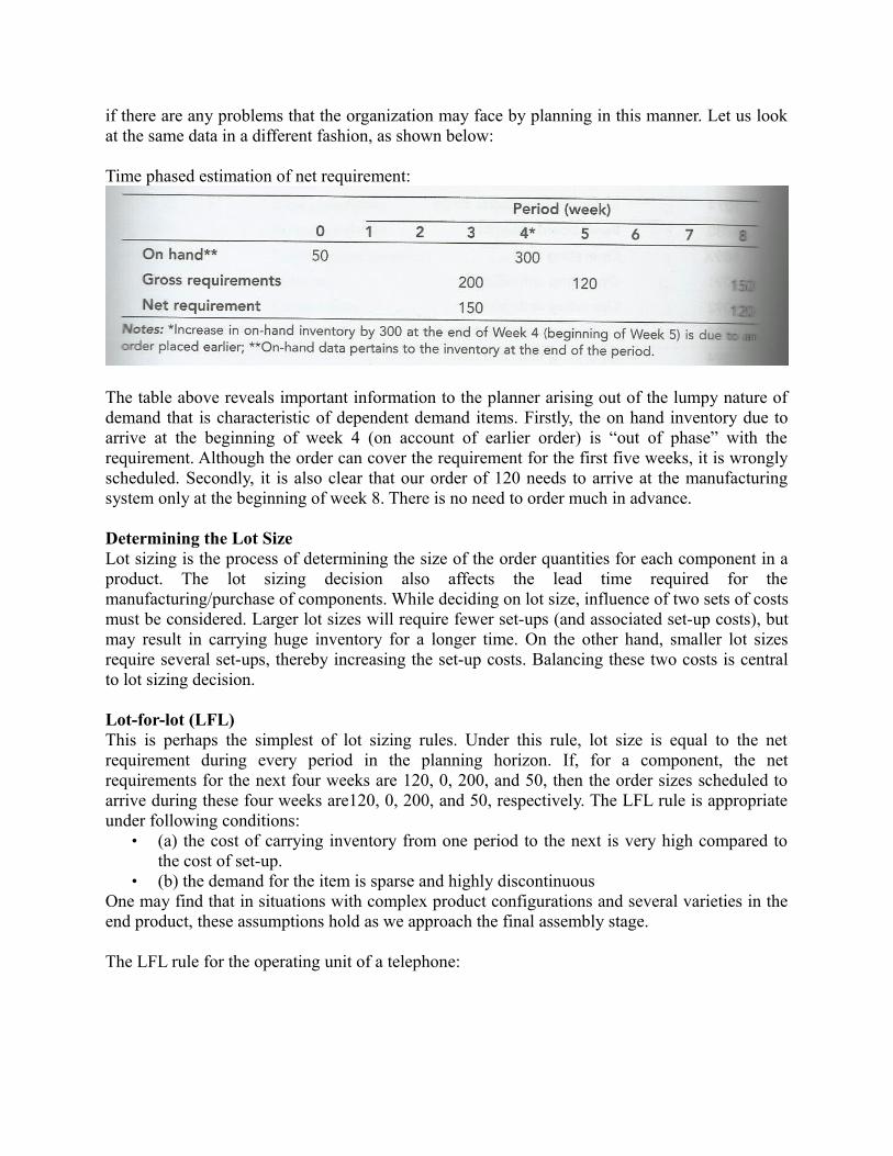
if there are any problems that the organization may face by planning in this manner. Let us lookat the same data in a different fashion, as shown below:

Time phased estimation of net requirement:

The table above reveals important information to the planner arising out of the lumpy nature ofdemand that is characteristic of dependent demand items. Firstly, the on hand inventory due toarrive at the beginning of week 4 (on account of earlier order) is “out of phase” with therequirement. Although the order can cover the requirement for the first five weeks, it is wronglyscheduled. Secondly, it is also clear that our order of 120 needs to arrive at the manufacturingsystem only at the beginning of week 8. There is no need to order much in advance.

Determining the Lot Size Lot sizing is the process of determining the size of the order quantities for each component in aproduct. The lot sizing decision also affects the lead time required for themanufacturing/purchase of components. While deciding on lot size, influence of two sets of costsmust be considered. Larger lot sizes will require fewer set-ups (and associated set-up costs), butmay result in carrying huge inventory for a longer time. On the other hand, smaller lot sizesrequire several set-ups, thereby increasing the set-up costs. Balancing these two costs is centralto lot sizing decision.

Lot-for-lot (LFL) This is perhaps the simplest of lot sizing rules. Under this rule, lot size is equal to the netrequirement during every period in the planning horizon. If, for a component, the netrequirements for the next four weeks are 120, 0, 200, and 50, then the order sizes scheduled toarrive during these four weeks are120, 0, 200, and 50, respectively. The LFL rule is appropriateunder following conditions:

• (a) the cost of carrying inventory from one period to the next is very high compared tothe cost of set-up.

• (b) the demand for the item is sparse and highly discontinuous One may find that in situations with complex product configurations and several varieties in theend product, these assumptions hold as we approach the final assembly stage.

The LFL rule for the operating unit of a telephone:

Fixed Order Quantity (FOQ) In this rule, irrespective of the nature of the demand, orders are always placed for a fixed orderquantity. Orders are scheduled such that they arrive at the first point of demand. The next order isscheduled to arrive when the first order is insufficient to meet the net requirements for the period.The procedure continues in this fashion until the requirements for the entire period are coveredby the orders as shown in the figure below:

In this case, the first point of demand for the operating unit occurs during week 3. Therefore, anorder quantity of 300 (FOQ) is scheduled to arrive at the beginning of the week. This quantitysatisfies the net requirements until week 6. Therefore, the next order of 300 is scheduled to arriveat the beginning of week 7. Different methods can be used to compute the fixed order quantity(FOQ). One method is to estimate the economic order quantity on the basis of set-up/orderingcost and carrying cost. FOQ provides an alternative perspective to the carrying cost-orderingcost trade-off. In general, when the unit value of the item is low and demand for the item is moreor less stable, it is appropriate to use this rule. Items that are at the lower end of a productstructure share a greater degree of commonality among numerous end-product variations.Therefore, the demand is likely to be continuous justifying the choice of FOQ rule.

Periodic Order Quantity (POQ) In this method, an order is placed such that it covers the requirements of P periods. It does notmean that we should place an order quantity during every P period. It only suggests that if weplan an order at a particular time, the quantity should cover the net requirements of P successiveperiods. The choice of P could be made in alternative ways. One method is to use the review

cycle. If an organization reviews decisions every two months, it could be an appropriate time toalso plan the orders. Another method is to use the economic order quantity (Q*) and the averagedemand during the period to arrive at P. Number of periods P = (Q*) / average demand duringplanning period

Implementation of POQ rule for operating units with P = 3:

The timing of orders in dependent demand items is very crucial. Errors will have a cascadingeffect right through the product structure. One important aspect is to incorporate the lead timeinformation in the planning exercise. Accurate computation of component lead times is thereforeimportant in obtaining realistic schedules for the components.

MRP LogicMaterial Requirements Planning (MRP) is a structured approach that develops schedules forlaunching orders for materials in any manufacturing system and ensures availability of these atthe right time and at the right place. It uses the basic building blocks of resources planning todevelop these schedules. The figure below shows the core logic of MRP process, its input, andoutput:

As shown in the figure, four key processes drive the MRP procedure. These processes occur in acyclic fashion. The first process is the “net” process. The MPS for the end product providesinformation on the gross requirements for the end product. By utilizing the information availablein the inventory records, the “net” process computes the net requirements for the end product.The second process is the “lot” process. Once the net requirements are computed, the lot sizingrule is used to schedule planned receipts of the product. The third process is the “offset” process.Once the planned receipts are identified, lead time information is used to offset and obtainplanned order releases for the product. The planned order releases are either work orders for amanufacturing shop to assemble as many components as per the schedule or a purchase order toobtain sub-assemblies from outside.

Once these three processes are completed, the requirements for the end product are estimated andorders are scheduled. Then the next step is to cascade the process down the product structure andrepeat the procedure with all the components at the next level in the product structure. Thisprocess is the last in the cycle denoted as “explode”. In order to perform the “explosion” process,BOM data is required. The planned order releases of a parent creates dependent demand for theoffspring as specified in the BOM. This becomes the gross requirements for the offspring. Theprocedure continues iteratively, level by level, until the lowest level is reached and all componentschedules are determined.

Therefore, the key inputs for the MRP processes are MPS, BOM, inventory status, lead timedata, and lot sizing rule. Each one of these is important in accurately determining the quantityand timing of the material requirements. As we proceed through the lower level of components,two types of outputs are generated from the MRP system. The first output is a work order. workorder are generated for items that are manufactured in-house. In our telephone example, wewould have generated work orders for base set and handset assemblies as they are likely to bedone in-house. The second output is a procurement notice. Procurement notices are generated foritems that are bought from outside and directly used in the assembly. It triggers the purchaseordering process. In our telephone example, it is possible that the manufacturer might directlysource connecting cables and jacks instead of producing them in-house. The outcome of MRPprocess is a procurement notice.

Using the MRP SystemThe most significant impact that a well designed MRP system could provide to an organization isthe reduction in inventory. MRP systems were first developed in the early 1960s andorganizations that started using them reported dramatic reductions in their inventory. The reasonsare obviously related to the logic of exploiting the particular characteristics of dependent demanditems. Using traditional EOQ based inventory control system will often result in havinginventory when not required. The other advantage is the increased visibility of items and theirdependencies through a BOM representation of products being manufactured. Further, it couldpossibly inculcate a certain discipline in the planning process.

Despite the simplicity and initial success, MRP installations faced several problems afterimplementation. These were; The data integrity is low. If the lead time data is wrong, organizations may either have too muchinventory or frequent shortages. Similarly, if the inventory status is wrong, it could jeopardize

the entire computation. Users did not have the discipline of updating the required databases asand when changes were taking place elsewhere in the organization. If the R & D departmentcreates new design and revisions in existing product design, this data needs to be incorporated inthe BOM file. There are uncertainties associated with several issues that lie outside the control ofthe people and the system. For instance, bad supply management resulting in many uncertaintiesin lead time and quantity delivered etc. Due to these reasons, the predictions made by MRPsystems may often turn out to be less accurate. This could also result in several productionschedule changes and consequent delays in the downstream supply chain. Moreover, there arealso other limitations in using MRP system. The amount of computation involved in generatingcomponent-wise schedules for the planning horizon is large. Real-life examples requirethousands of iterations that consume time. Instead of the speed and accuracy increasingcontinuously, this issue still merits some attention and puts realistic limits to the frequency ofgeneration of MRP schedules.

Therefore, an organization needs to incorporate certain aspects into the MRP planningframework to minimize problems arising out of these issues. Alternative methods are available tore-run an MRP system and they have implications on the accuracy, cost, and time pertaining tothe exercise. However, there are methods available to handle some of the uncertainties in thesystem and thereby reduce the risk of shortage. But such alternatives have cost implications aswell.

Updating MRP SchedulesIn actual situations, plans become obsolete over time due to several changes in the environment.For example, a customer might have cancelled an order or amended the order quantity anddelivery schedule; a supplier could have defaulted in the supply schedule. Similarly, there couldhave been some unexpected disruptions in the manufacturing and assembly schedules within themanufacturing system. In such cases, the MRP and the schedules for order releases and purchasebecome inaccurate and call for re-planning. Therefore, the critical to resolve while using theMRP system is the frequency with which the MRP systems are re-run.

We will now discuss certain methods available for updating schedules in MRP: RegenerationIn this method, the MRP system is run from scratch. Based on the changed information, one canstart from level 0 and run the MRP logic right up to the bottom level, amounting to 100%replacement of existing MRP. Net Change In this method, instead of running the entire MRP system, schedules of components pertaining toportions where changes have happened are updated. Clearly, net change method of updatingMRP schedule modifies only a subset of data as opposed to regeneration. Therefore, it is likely tobe computationally more efficient than the regeneration method. Moreover, it may be possible torun it in frequent intervals.

The decision to use net change or regeneration depends on the magnitude of changes that occurin the organization. If the number of changes tend to be large, then it is better to use regenerativemethod for updating MRP schedules. If the number of changes is small, then it is better to use

net change method. The cost of running an MRP system and the number of changes happening inthe planning horizon influence the type of updating procedure and the frequency of updation

Safety Stock and Safety Lead Time Uncertainties in the system that are outside the control of an MRP system is a reality, thatorganizations need to face and plan for. Generally two types of uncertainties are prevalent:

• Quantity of components received, and • The timing of receipt.

Poor quality of input material could result in quantity loss on account of rejections. Alternatively,reliability of suppliers may also result in uncertainty in quantity. In the case of componentsmanufactured in-house, there could be uncertainty in supply quantity due to changes in the batchquantity of upstream stages. Therefore, it may be desirable to plan for a safety stock to absorbthese uncertainties.

The inclusion of safety stock in MRP computation is fairly straightforward. At the time of“netting” the requirements, an order is scheduled to arrive when the on-hand inventory fallsbelow zero. Instead, the order needs to be scheduled when the on-hand inventory falls below thesafety stock. The figure below shows the MRP schedules for a component both without anysafety stock and with a safety stock of 50.

MRP schedules without safety stock and with safety stock of 50:

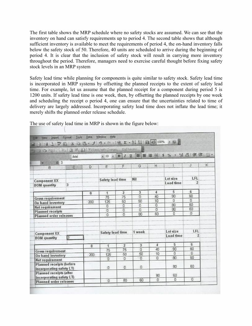
The first table shows the MRP schedule where no safety stocks are assumed. We can see that theinventory on hand can satisfy requirements up to period 4. The second table shows that althoughsufficient inventory is available to meet the requirements of period 4, the on-hand inventory fallsbelow the safety stock of 50. Therefore, 40 units are scheduled to arrive during the beginning ofperiod 4. It is clear that the inclusion of safety stock will result in carrying more inventorythroughout the period. Therefore, managers need to exercise careful thought before fixing safetystock levels in an MRP system

Safety lead time while planning for components is quite similar to safety stock. Safety lead timeis incorporated in MRP systems by offsetting the planned receipts to the extent of safety leadtime. For example, let us assume that the planned receipt for a component during period 5 is1200 units. If safety lead time is one week, then, by offsetting the planned receipts by one weekand scheduling the receipt o period 4, one can ensure that the uncertainties related to time ofdelivery are largely addressed. Incorporating safety lead time does not inflate the lead time; itmerely shifts the planned order release schedule.

The use of safety lead time in MRP is shown in the figure below:

Capacity Requirements Planning (CRP)Capacity requirement planning (CRP) is necessary to ensure that what needs to be producedduring a period can in fact be produced. CRP is a technique that applies logic similar to MRP toaddress the capacity issues in an organization. Similar to MRP, CRP develops schedules forplanned releases of capacities to specific work orders as identified in an MRP schedule. Theoutput of an MRP becomes the basis for the CRP exercise. The notion of dependency appliesvery well to capacities also. Every manufacturing process generates a dependent demand for theresources involved in the conversion process. CRP systems employ the detailed schedulegenerated by an MRP system as the basis for capacity planning.

Just like MRP system, CRP system also uses the capacity status as the starting point for the“netting” process, as shown in the figure below:

There are similarities between MRP and CRP and therefore organizations use logic similar tothat of MRP for performing CRP. However, there are certain important issues that one needs tounderstand about MRP-CRP-MPS interfaces. In a simple hierarchical mode, MPS will driveMRP and MRP in turn will drive CRP. If both the schedules are feasible, then the plan isfinalized. On the other hand, if there are mismatches between capacity and material schedulesdue to non-availability of capacity to meet the MRP schedule, then it calls for a few iterations ofthe process. The MRP schedules are first modified to obtain feasible MRP and CRP schedules.However, if this is not possible, then the MPS is modified until feasible schedules are obtainedfor both material and capacity.

Distribution Requirement Planning (DRP)The logic of MRP is sufficiently general to apply to several other areas of business. Oneextension of MRP is to plan distribution inventories in the downstream supply chain, consistingof depots and stocking points at the dealer level. Consider a downstream supply chain consistingof a factory warehouse, four distribution centers, and twenty dealers, geographically spread outin the country. The demand t the dealers’ level aggregates up in the chain and eventually reaches

the factory warehouse. Transporting the products through supply chain involves a certain leadtime. Further, the products are transported in some preferred lot sizes. In general, orderingdecisions happen based on a periodic review of stock and the emerging demand. This causes thedemand at the next level in the supply chain to be lumpy. Therefore, it calls for time phasing ofthe planning process.

The logic of MRP can be easily applied to planning distribution requirements. Using time phaseddata, organizations could schedule the planned receipt of products at various points in the supplychain and offset these by the required lead time to arrive at planned order releases for dispatch ofmaterial to the demand points. A dealer may review the inventory on hand and the likely demandduring the planning period and arrive at the net quantity to order. Based on lot-sizingconsiderations, he may lot the order and determine and determine the planned receipts. Furtherby offsetting the order to the extent of lead time required for receiving the order, he may arrive atthe planned order releases for each period. This becomes the gross requirement for thedistribution centers. The entire process could be repeated at the distribution centers and theplanned order releases of the four distribution centers eventually influence the MPS at thefactory.

A DRP exercise will help organizations and their supply chain partners to jointly plan and reduceinvestment in inventory in the supply chain. They will be able to respond to changes in thedemand and have a cost-effective operation. They will also be able to offer high level of serviceto their customers. However, unlike MRP exercise, DRP exercise relies on key informationpertaining to planned order releases outside the domain of the organization. Retailers should bewilling to share with dealer the planned order releases and their estimates of upcoming demand,for better planning. Similarly, dealers need to share similar information with the manufacturer. Ifthe information exchange is not proper and there is no data integrity, then the value of the entireexercise will be severely undermined. It will eventually result in inventory build-up or shortages,poor service, and increased costs of operation in the supply chain.

Manufacturing Resources Planning (MRP II)It was quite logical that newer systems were developed to expand the application of MRP, intoother domains of business where dependency relationships exist. In the 1980s, organizationsbegan to incorporate several modules in the MRP systems. This extended version is known as“Manufacturing Resources Planning (MRP II). A typical MRP II system consists of followingmodules:

• Business planning • Purchasing • Forecasting / demand management • Inventory control • Order entry and management – Shop floor control – Master production scheduling (MPS) – Distribution requirements planning (DRP) – Material requirements planning (MRP) – Service requirements planning (SRP) – Capacity requirements planning (CRP)

– Accounting Thus, MRP II covers all activities from business planning to servicing the customer. Inreality, business planning exercise triggers dependency relationships for all resources in anorganization. The forecasting/demand management module and the order entry systemessentially interface with the outside world and bring recent information into the planningsystem.

Based on these, production planning, MPS and other requirements planning can be done. Sincethe outcome of these exercises is to procure all items and services from outside and perform thein-house activities as per plan, the relevant modules are also included to close the gap.Essentially, the focus is on planning for all the resources that an operations system requires. Theadvantage of MRP II lies in the ability to provide numerous feedback loops between differentmodules and minimize re-planning on a piece-meal basis. As more and more gaps are closed, itpromotes a centralized approach to planning and promises to bring additional benefits arising outof integration.

Enterprise Resource Planning (ERP)ERP is an organization-wide planning system that utilizes some common software and anintegrated database for planning and control purposes. ERP embeds all the organizationprocesses into the software and creates a work flow mechanism such that different organizationalplayers engaged in planning and control of a variety of activities can make use of the system.Viewed alternatively, ERP I a mammoth transaction engine that runs on some common software.Since activities in an organization typically have hundreds of processes comprising of thousandsof activities. The software is split into modules representing functional domains. Each modulehas a set of inputs, processes, and outputs. Further, each module is closely interconnected withseveral other modules. The power of ERP software lies in its ability to manage these interfaceswell, thereby providing tighter integration.

The role of ERP on interfacing functional areas of business:

The following are the typical modules in ERP software: • Sales and distribution • Production planning • Logistics • Accounts payable/receivable, treasury • Operational (shop floor) control• Purchasing • Finance and cost control • Human resources

In addition, other tools are also available for generating web interfaces, coding and programgeneration routines, data import/export, and a library of best practices from which anorganization could choose processes for implementation.

A wide number of software options are available for ERP. The most popular among them includeSAP, Oracle, Rameo systems, Peoplesoft, and ID Edwards. The heart of ERP is the organization-wide integration of several activities. This ranges from integration of functions to markets,divisions, plants, products, and customers across the globe. The greatest benefit to theorganization from implementing ERP is its ability to link various functional areas of businesstightly through the software. The ERP software will ensure that with the input new informationin each of these modules, all the modules will get automatically updated with this information.ERP promises to cut down cycle time, transaction costs, layers of decision making, and therebyimprove responsiveness and flexibility. An ERP system could be the backbone of ITinfrastructure for an organization. All these will eventually lead to improving competitiveness ofthe organization at the market place.