Module 1 – Viewing Digital Data in...

An Introduction to Geographic Information Systems (GIS)

An Introduction to Geographic Information Systems (GIS) using ArcGIS 9.x

by

Marcel Fortin, GIS and Map Librarian, University of Toronto Libraries, 2010 [email protected]://www.library.utoronto.ca/maplib/

© Marcel Fortin, GIS and Map Librarian, University of Toronto Libraries 2010 1

http://www.library.utoronto.ca/maplib/

mailto:[email protected]


Module 1 – Getting to know ArcMap : using a pre-made “map” or “project file”

Objective of Module: Learn to use ArcMap GIS software, use a pre-made project file (map), zoom in/out of a map, experiment with scale, label map data, and get

information from map data

1) Start by downloading the datasets required for these modules from http://maps.library.utoronto.ca/dataut/arcdata/arcdata.zip and save this file in the c:\user\documents\ area of your computer

2) Unzip the zipped file by right-clicking on it and choosing 7-zip Extract Here3) Open ArcMap by selecting it from the Start menu

4) Once, in ArcMap, Click on or or use the File menu and select Open…

5) Navigate to C:\user\documents\arcdata\Ontario\ highlight ontario.mxd (this is called a map project file and contains the information about layers/features that make up your map), click on open. The map below will appear on screen.

Table of Contents

6) turn all layers off one at a time by clicking in the Table of Contents7) turn all layers on one at a time by clicking


Data View

http://maps.library.utoronto.ca/dataut/arcdata/arcdata.zip


8) turn all layers off by right-clicking on Layers and selecting Turn All Layers Off

9) turn all layers on by right-clicking on Layers again andselecting Turn All Layers On

10)Zoom in by selecting the tool and click in the center of the map area a few times

11)Zoom out by selecting the tool and click a few times in the center of the map area

12)Go back to the full-extent of the map area by clicking on the globe

13)Click hold the zoom-in tool ; draw a box around Southern Ontario as in the image below



14)Change to a specific scale by entering 1:2,000,000 in the scale box

15)View previously used and set scales by clicking on the scale box selection tool on the right of the box and select a different scale

16)Right-click the oncoastline layer in the table of contents on the Table of Contents on left side of the screen and select Zoom to layer

17)You will notice that you have been sent to the only “coastline” Ontario has on Hudson’s and James Bay

18) Highlight the oncoastline layer by clicking on the word oncoastline as shown in this image



19)Click once on the dotted line underneath the word oncoastline.

20) A symbol selector box will appear. Scroll down using the scrollbar and select the option Coastline. Select a colour for your line using the Color option on your right; and the Width option to select a line thickness at 2. click on OK once you have made a selection.

You will notice that the colour and visibility of the coastline on the map is now quite different.

21)Go back to the full-extent of the map/data by clicking on the globe22)Click on 23)As you move in the map view you will notice the coordinates of where the mouse is

at the bottom right of the screen

24)Zoom to Southern Ontario again to where you think you could find TorontoHint:

25)Try and find the approximate north and south coordinates for where you think the Toronto city centre is located. X(longitude)_________ West, Y(latitude)___________ North



26)Now bookmark your zoomed in area using the Bookmarks menu and selecting Create…

27)Give your bookmark the name Toronto City Centre, click on OK. If you are asked to replace the previous Toronto bookmark, click on “Yes”.

28)Go back to the full-extent of the data/map by clicking on the globe

29)Go back to your bookmark by selecting it in the Bookmarks option of the View menu

30)Go to Algonquin Park by selecting the bookmark already created for you called “Algonquin Park”.



31)Get information on a layer by clicking on . Select the Onparks Layer from the Identify from: box in the new Identify screen. Use your cursor and click on the park on the map (it is in green). Information about the area clicked will appear giving you information on the area.

32)Close the Identify Results box

33) Highlight the onparks layers by clicking on it in the Table of Contents on the left-hand side of the screen

34)Right-click on the layer and select Open Attribute Table



35)You will notice a table of attribute information. Notice the NAME column and the entries? You will now use this column to label your layer on the map. Close this table.

36) Right-click on the onparks layer again but now select Properties. Select the Labels tab. Under the Text String Label Field: option, select NAME. Click on OK.

37)Right-click on the onparks layer again and select Label Features.



Module 2 – Creating a printable mapObjective of Module : use the layout view of ArcMap and create and export a printable map complete with scale bar, legend, and north arrow

1) Bring up the full-extent of the last module by clicking on 2) To start creating a printable map of your Ontario.mxd project use the View menu

and select Layout view (NOTE: we will not be printing out any paper maps, only a digital one)

3) Highlight the map area as below by clicking once on the map, click on the box, move it, and stretch to a smaller portion of the page.

4) Using the main zoom tool, pan and zoom to Southern Ontario (CAUTION: not the layout zoom tool )



5) Under the Insert menu, select the Scale Bar… option

6) Highlight Scale Line 1 and press OK

7) Place the scale bar in the bottom left corner of the map using the mouse

8) Double-Click on the scale bar and select Kilometersunder the Division Units option. Press OK.



9) Using the Insert menu, select the North Arrow… option

10) Highlight a North Arrow and click OK. Place the North Arrow in the bottom right corner of the map

11)Using the Insert menu, select the Legend… option

12) In the Legend Wizard box, select Set the number of columns in your legend to 4 and click on Next

\



13) Replace the Legend Title with the legend name Ontario, or any title you want to give your map

14) Click on Next three more times until you reach a box that has the option Finish at the bottom. Click on Finish

15)Place your Legend above the North Arrow and the Scale Bar using your mouse cursor

16)Under the File menu, select Export Map…

17)Navigate to where you want to save your digital map, starting in the directory: C:\user\documents\arcdata\



18)Choose a name for your map and select the pdf or JPEG format. Click on Options…, highlight the tab General, select 300 dots per inch (this is the resolution of your map) in the box. Click on Save.

19)Navigate to where you saved you file using Windows Explorer and double-click on your newly created PDF or JPEG exported map.



Module 3 – Loading Digital Map Data (Raster1 and Vector2) and working with datums3 and projections4

Objective: Manipulate data files to fit with one another and to get comfortable with combining and moving around layers in the Table of Contents.

1) To get out of the Layout view, using the View menu, select Data View

2) Create a new project by clicking on 3) Click on Yes to Save changes to Ontario.mxd? pop up box. It is important to

ensure, when working with GIS projects like these, to save often and to save changes made to views and additions of data files, labels, etc.

4) Open a new map layer by clicking on 5) Navigate to C:\user\documents\arcdata\toronto\6) Select the layer file tostreets.shp, click on Add. Note that a file with an extension

.shp refers to what is called a “shapefile” in GIS parlance. (Note that a shapefile is actually made up of several files…up to about 13 of them in fact. The tostreets.shp file is actually made up of six files but only the tostreets.shp is seen by the ArcMap interface).

7) Add layer/shapefile tocensus.shp (same as step 4)

1 Data source that uses a grid (equally sized square cells arranged in rows and columns) structure to store geographic information such as longitude and latitude.2 Coordinate-based data structure used to represent linear geographic features. 3 Parameters and control points used to accurately define the three-dimensional shape of the earth. It defines part of a geographic coordinate system.4 Mathematical formula that transforms locations between the earth’s curved surface and a map’s flat surface. Projections cause distortions in spatial properties.



8) A Warning box will appear telling you that two different coordinate systems were used for the two different files. Vector files can be transformed on the fly by clicking on Close. Click on Close now.

9) In the data view, note the coordinates in the bottom of the screen. How close were you in module 1 to finding the coordinates for Toronto?

10)Click-hold the tocensus layer and move it above the other layer like in the image below using your mouse. This is the method used to overlay one dataset over another. You will notice that the streets disappear. Move them back to the top using this same method

11)Using add the low-resolution air photo toronto99.tif (NOTE: Highlight the name of the image and click on Add. Do not double-click on the image)


Your map should look like the following


12)The following message box should appear telling you that the data does not have any spatial reference information attached to it; click on OK.

You will notice that no air photo appears in the map screen. This is because the image has a different coordinate system and projection from our shapefile (vector layers). Raster images cannot have their projection and coordinate systems changed on the fly, unlike vector data, unless the image is accompanied by a projection (.prj) file. This, unfortunately, is rarely the case when downloading raster imagery.

13)Ensure the Display option is selected at the bottom left of your Table of Contents

14)Click-hold the image layer toronto99.tif and move it above the other layers like in the above steps. Unlike previously, you will note that you are still not able to see the image just loaded.

15)Right-click on Layers and select Properties.

16)In order to be able to view and use the image with these datasets, the coordinate system will have to be changed to match that of the image’s coordinate system. In the Data Frame Properties box that appears (see below) select the



Coordinate System tab. you will notice in the box below that the current coordinate system we are using is GCS_Assumed_Geographic (degrees, minutes, seconds) and that the datum is North American 1927. The air photo datum, however, is North American 1983 and its projection is UTM Zone 17.

17) Select Predefined by highlighting , and select Utm

18)Next select, Nad 1983->NAD 1983 UTM Zone 17N

19)Click on OK, and YES to the Warning box again 20)You will notice that the map is now projected differently and that the air photo

now appears on the map screen.



21)Right-click on the toronto99.tif filename and select Properties…22)Select the Symbology tab, tick the Display Background Value: box and enter

255 in the three (R,G,B) boxes. Select the colour selection drop down menu and select No Color. Click on OK. This will make the image colour 255 (outer image) transparent.

23)You will now notice that the air photo does not have extraneous white pixels outside of its boundaries

24)Add the air photo layer C:\user\documents\arcdata\toronto\uoft99.tif25)Right-click on this layer and click on Zoom to Layer26)You will notice the difference in resolution between the two images by the pixels

on the outer edges of the screen.



27)Using the tool zoom in closer and closer into this image. 28)Click-hold the tostreets layer and drag it above the other two layers

29)Zoom into the center of the uoft99 image. Notice how the streets in this layer align with the streets on the image.

30)Click-hold the tocensus layer and drag it to just below tostreets in the Table of Contents (make sure this layer is clicked on)

31) You will notice that the air photo images now disappear. This is because the tocensus layer is a polygon feature, which allows for adding different colours to “areas” (polygons).



32)Let’s change that option to no colour and let’s change the outline of each polygon. Click once on the colour box below the tocensus layer.

33)In the symbol select box click on the Fill Color: option and select No Color

34)Change the Outline Width to 2 and the Outline Color to green

35)Move the image uoft99.tif to the top of the list. All layers underneath should disappear.



36)Right-click on the taskbar at the top and make sure the Effects option is clicked on

37)Select uoft99.tif from the list in the Layer: menu bar

38)Right-click on the uoft99.tif layer and select Zoom to Layer

39)Using the little jug on the Effects task bar, select a transparency of about 49%. Now look at the image. Play around with a variety of transparency percentages.

40)Save your project as C:\user\documents\arcdata\toairphotos.mxd using the File->Save As… option



Module 4 – An Introduction to Thematic Mapping5

Objective: Learn to make a Thematic Map. Learn to link data tables together. Get comfortable with the database concepts of GIS

1) Click on to create a new map file2) Add data to the new map file by clicking on 3) Add the layer C:\user\documents\arcdata\toronto\tocensus.shp4) Right-click on the tocensus layer and select Open Attribute Table

5) You will notice that there is some attribute data in this database, but no variables that can be mapped thematically. We are looking for numbers/statistics associated to each polygon in order to map a specific theme.

6) Using , add the census database file C:\user\documents\arcdata\toronto\tolanguage.dbf (this file was extracted from a Statistics Canada database at http://www.chass.utoronto.ca/datalib)

7) You will notice that nothing is drawn on the screen. This is because this is simply a database and not a GIS file.

8) Right-click on the tolanguage file and select Open.

9) Repeat step 4. Compare the database fields for both files (hint, look at the GEOGRAPHY field). Do you notice any similarities between the two databases? If not, right-click on the CTNAME field in the tocensus shapefile layer and select Sort Ascending

5 A thematic map is a map which displays selected kinds of information relating to specific themes, such as soil, land-use, population density, crops, etc.



10) You will notice now that the first record in the CTNAME field is the same record in the GEOGRAPHY field in the tolanguage database

11)Close both database windows by clicking on the in the top right corner of both tables

12)Now we must join the two tables together to be able to map the data in the census table. Right-click on the tocensus layer, select Joins and Relates -> Join…



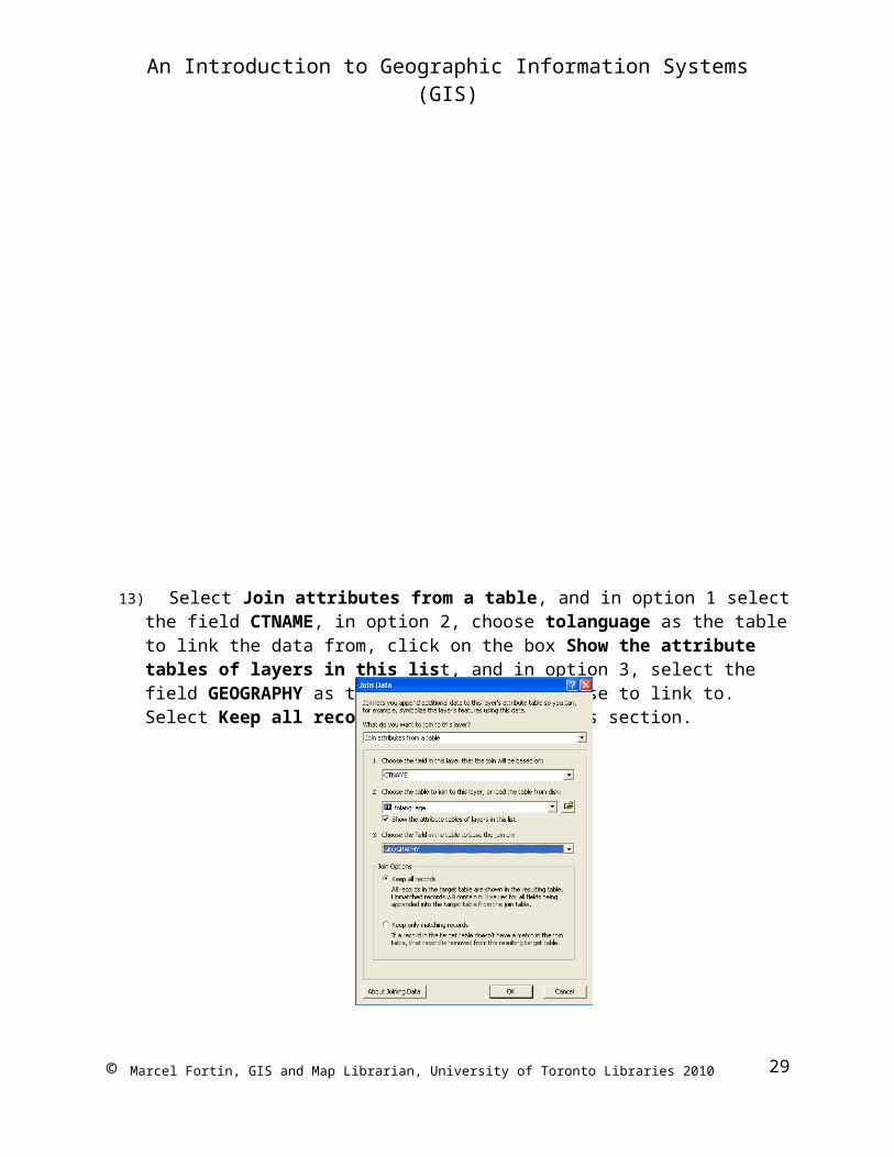
13) Select Join attributes from a table, and in option 1 select the field CTNAME, in option 2, choose tolanguage as the table to link the data from, click on the box Show the attribute tables of layers in this list, and in option 3, select the field GEOGRAPHY as the field in the database to link to. Select Keep all records in the Join Options section.

14)Notice that nothing different occurs on the screen15)Repeat step 4. Notice anything new in the table? Scroll to the right of the table.

You should now see the data from our database incorporated into our map layer. Close this window.



16)Double-click on the layer tocensus. Click on the Symbology tab. Click on Quantities on the left and then Graduated colors. In the Fields Value: option, select Value: tolanguage.TOTAL_POPU. Under Classification, select 6 Classes. Click on the Show class ranges using feature values option. Click on OK. Your map should look like the image on the right.

17)To calculate the population density, repeat the last step, but this time normalize the display with the field tocensus.LAND_AREA_

18) Repeat the last step but this time use Graduated symbols and use the same option as in the image below.



19)Repeat again but this time use the Dot Density option and use the variables as in the image below. Highlight tolanguage.TOTAL_POPU in the Field Selection box

and click on to select this field. Select the Dot Size to be 1 and Dot Value as 50, click on OK.

20) Save this project C:\user\documents\arcdata\tocensus.mxd but do not exit out of the project.



Module 5 – Manipulating GIS datasetsObjective: Use Structured Query Language (SQL) statements to Query and create

new data from attributes associated to GIS layers.

1) Using the project from the previous module, right-click on the tocensus layer and select Data->Export Data… to create a new shapefile incorporating the previous census shapefile and the census database into one editable layer/file.

2) Export the file as shown in the image below using the default values (make sure the “Export:” option is set at “All features” in the pop-up box, save the file in the directory C:\user\documents\arcdata\census\. Click on OK.

3) If the system asks for you to overwrite the previous shapefile called Export_Output.shp, click on Yes.

4) Answer Yes to the next box to add the data to your current project.

5) Right-click on the original tocensus layer and select remove. Repeat for the file tolanguage



6) Right-click on your new shapefile Export_Output and select Open Attribute Table… You will notice that all your attribute data from your linked database is now part of this new layer.

7) We now want to add a new field to store our calculated population density. Click on Options at the bottom of the table and select Add Field…

8) Give your field the name density, select the type as Short Integer, and in the Precision option type in 10 for the size of the field.

9) Click on Options in the table menu at the bottom, and select Select By Attributes…



10)In order to populate our field with our calculation, without incurring errors, we need to perform a search for all entries with values greater than 0 (a few census areas have no official populations attached to them and remove any null values). Double-click on the field TOTAL_POPU, then click once on > and type in 0 (zero) to end up with the expression SELECT * FROM Export_Output WHERE: “TOTAL_POPU” > 0 click on Apply.

11)Click on Selected. This will list only the areas found with the previous operation and take out the areas with no population numbers or null values for our next calculation.

12)Right-click in the tool bars area at the top of the software and make sure the Editor option is on.



13)Using the Editor menu select Start Editing

14) Right-click on the density field (where the field is listed as “density”) in the database and select Field Calculator…

15) Calculate the population density in Toronto by double-clicking on the field TOTAL_POPU then click once on “/” and double-click on the field LAND_AREA_ click on OK. Now explore the density field, you will see that you have just filled it with data by applying the population density equation of Population divided by land area.

16)Using the Editor option, select Stop Editing. Answer yes to the pop-up box asking if you want to save your edits.



17)Double-click on the layer Export_Output. Click on Quantities on the left. In the Fields Value: option, select density. Under Classification, select 6 Classes. Click on the Show class ranges using feature values option.

18)Select a Color Ramp of your choice

19)Click once on the first Range. Enter 0 to display population densities with no numeric values.

20)Double-click on the Symbol box and select for Fill Color: No Color. Click on OK.



21)Zoom into the downtown area of Toronto. You can easily see the highest density area and the areas where there is no data (in white).

22)To find the highest density area in Toronto, right-click on the Export_Output layer and select Open Attribute Table…

23)Scroll right to your density field, right-click on it, and select Sort Descending

24)Highlight the top record by clicking on the box on the left of the record. Close the database window.

25)Right-click on the Export_Output layer, go to the Selection option and click on Zoom to Selected Features.



26)Your map should now look like this.

27)Add the layer C:\user\documents\arcdata\Toronto\tostreets.shp.28)Right-click the tostreets layer and select Label Features. What are the streets

that make up the boundaries for this most densely populated area of Toronto? ________, ________, ________, ________

29)Save your project as tocensus.mxd



Module 6 – Creating your own geographic dataObjective: Learn to manipulate simple datasets that can be mapped out.

1) Using Windows explorer, navigate to C:\user\documents\arcdata\census\2) Open the text file census.txt by double-clicking on it.

3) Add the following three lines at the bottom of the file (exactly as you seen them):

Yukon Territory,28674,14445,14235Northwest Territories,37360,19115,18245Nunavut,26745,13840,12910

The source for this data is the Census of Canada, 2001 (www.estat.ca)

4) Once you have typed the information for the territories, exit and save the file to C:\user\documents\arcdata\census.txt. (NOTE: Make sure you are saving the data as a text file and not anything else such as a Microsoft Word document if using Word as your editor).

5) In ArcMap, create a new project by clicking on . Add the u:\user\documents\arcdata\canada\provinces.shp layer and the text file you just edited census.txt.

6) Right-click on your census.txt file and select Open7) Your file is considered a database file by Arcmap and should look like one,

complete with field names (first line of your comma-separated text file).8) Join the provinces layer and your new database like you did in module 49) Now create a new map with the provinces labeled with the total population for

each province by double-clicking on the provinces layer and selecting population as the Label Field:



10)Now create a new thematic map showing graduated colours for the total population, then the female population

Adding X,Y Location Points

11)In ArcMap, open the project C:\user\documents\arcdata\ontario\ontario.mxd, you do not need to save the last project.

12)Go to the Algonquin Park bookmark

13)Add the text file called C:\user\documents\arcdata\gps\gpspoints.txt (these points were downloaded from my Global Positioning System (GPS) unit.

14)Open this file’s attribute table by right-clicking on it and selecting Open15)You will notice that the file has two fields representing the data’s longitude and

latitude. These points can be mapped according to these coordinates combined together. Close this window.

16) Using the Tools menu select Add XY Data… or right-click on the layer and select Display XY Data…



12) If the table does not automatically open use the selection tab (circled below) to navigate to the database of GPS points C:\user\documents\arcdata\gps\gpspoints.txt. If not selected automatically, under the X Field: select longitude and under the Y Field: select latitude Click on OK.

13) You will notice that you now have a new layer with the same name as the gps points database but it will have the word Events next to it.14)Click on the dot below the gpspoints.txt Events layer

15) Select the triangle as a new shape, change the color to red and the size to 20.00 and click on OK.

17)The map should now look something like this

18)Using the information tool , click on the point inside Algonquin park.

19)Add the layer C:\user\documents\arcdata\on\lakes.shp



20)What lake is this point on?

Module 7 – creating your own polygon shapefile



Objective: learn to use the Edit functions of a GIS to create new georeferenced layers

1) open up ArcCatalog by clicking on in ArcMap2) Select the location of your new shapefile by highlighting on the left side of the

screen (Table of Contents) the folder where you would like to save your new shapefile.

3) In this case, save your file under C:\user\documents\arcdata\Toronto\4) Under File->New, select Shapefile

5) Give your new shapefile the Name: buildings and select the feature type Polygon, click on OK



6) Go back to ArcMap and using File->Open, open the project file C:\user\documents\arcdata\Toronto\buildings.mxd

7) Add your new shapefile: c:\arcgis\data\Toronto\buildings.shp8) Edit your shapefile by clicking on the Editor taskbar and select Start Editing

9) In the pop-up box you should see your new shapefile listed. Click on Start Editing

10)Select the sketch tool next to the Editor menu circled below

11)Start by drawing a polygon over the Robarts library building. To begin start at one corner and click, drag the line to the next corner and click again



12) Use several points to draw the building, once you are done, double-click on your last point.

13)If dissatisfied with your drawing, click on delete, if satisfied, click on the Editor menu and click on Save Edits

14)Zoom into smaller buildings and repeat steps 11 to 13 for two or three more buildings.

15)Save your edits every time your finish a building.16)Once done drawing, using the Editor menu, click on Stop Editing

17)Answer Yes to save your edits.

18)Right-click on your buildings layer and select Open Attribute Table.19)Using the Options tab, select Add Field



20)Give your field the name name. Click on OK.

21)Under Editor, select Start Editing22)In the new field of your database, start giving your buildings names

23)Once you have entered the building names, click on Stop Editing from the Editor taskbar.

24)Using the information tool , click on some of the buildings you drew.25)Repeat this entire module starting at but using a different feature class in

ArcCatalog (ie. point, line, etc) to draw roads, or represent trees, etc.



Module 8 – Georeferencing Raster Images of Scanned mapsObjective: learn the principles of georeferencing

1) In ArcMap, open the project C:\user\documents\arcdata\Toronto\georeference.mxd

2) Make sure that the georeferencing extension is on by right-clicking in the task bar area and selecting Georeferencing

3) Using the Georeferencing tool, select Layer: 004.jpg and under the menu Georeferencing, select Fit to Display and make sure that Auto Adjust is clicked on.

4) You will notice that the image 004.jpg now appears. This map is a 1910 Charles E. Goad Fire Insurance Plan. This is not a georeferenced image, but simply a scanned image of a paper map.

5) Select the Rotate tool and manipulate the image using your mouse so that the roads on the image are parallel to the roads in your GIS.



6) Your screen should look something like this image below.

7) Select the Control Points tool 8) Select the middle of the intersection of Avenue and Davenport on the image

(not the vector file) and click once. Drag the mouse to the same location on the vector file at the intersection of Avenue and Davenport.

9) You will notice the image has now moved over slightly. Repeat this operation for the Bedford Road and Bernard Street intersection and then the Elgin and Bedford intersection.



10)As the last point, you should choose the Avenue Road and Elgin intersection. Your image should now be completely georeferenced!

11)If your image is not matching the streets as you would like, you can eliminate some points by selecting the View Link Table icon:

12)If you need to delete a point, highlight it and press the delete key. Click on OK when done and resume adding control points to your image.

13)Once you are content with your image fit in your GIS, use the Georeferencing menu to select Rectifiy…



14)In the pop-up box that will appear, make sure you save the new rectified image in the C:\user\documents\arcdata\Toronto\ folder. You can give your new image any name you wish. Leave the other option at the default options. Click on OK.

15)Remove the image 004.jpg

16)Now insert your new rectified image into your workspace using the Add Data tool C:\user\documents\arcdata\Toronto\Rectify004.tif

This document: http://maps.library.utoronto.ca/docs/workshops/Modules1-8.doc Internally: \\Maps\data1$\www\html\docs\workshops\Modules1-8.doc


http://maps.library.utoronto.ca/workshops/Modules1-7.doc

Module 1 – Viewing Digital Data in...

Documents

Transcript of Module 1 – Viewing Digital Data in...