Modulation techniques and channel assessment for galvanic ...rx918912q/fulltext.pdfModulation...

Modulation Techniques and Channel Assessment for Galvanic

Coupled Intrabody Communications

A Thesis Presented

by

Fabian Abarca-Calderon

to

The Department of Electrical and Computer Engineering

in partial fulfillment of the requirements

for the degree of

Master of Science

in

Electrical and Computer Engineering

Northeastern UniversityBoston, Massachusetts

August 2015

To my grandfathers, Joaquın and Juan Felipe.

ii

Contents

List of Figures v

List of Tables vii

Acknowledgments viii

Abstract of the Thesis ix

Introduction 1

1 Intrabody Communications 31.1 Realm of Applications . . . . . . . . . . . . . . . . . . . . . . . . . . . . . . . . 41.2 Existing IBC Techniques . . . . . . . . . . . . . . . . . . . . . . . . . . . . . . . 6

1.2.1 Radio Frequency . . . . . . . . . . . . . . . . . . . . . . . . . . . . . . . 61.2.2 Ultrasound . . . . . . . . . . . . . . . . . . . . . . . . . . . . . . . . . . 71.2.3 Galvanic and Capacitive Coupling . . . . . . . . . . . . . . . . . . . . . . 8

1.3 System Overview . . . . . . . . . . . . . . . . . . . . . . . . . . . . . . . . . . . 9

2 Human Body Channel Characterization 112.1 Channel Models . . . . . . . . . . . . . . . . . . . . . . . . . . . . . . . . . . . . 12

2.1.1 Wave Propagation on Lossy Dielectric Medium . . . . . . . . . . . . . . . 152.1.2 Lumped Element Electric Circuit Model . . . . . . . . . . . . . . . . . . . 17

2.2 Experimental Assessment of the Channel Impulse and Frequency Response . . . . 202.2.1 Channel Probing . . . . . . . . . . . . . . . . . . . . . . . . . . . . . . . 21

2.3 Thermal Analysis . . . . . . . . . . . . . . . . . . . . . . . . . . . . . . . . . . . 25

3 Modulation Techniques for Galvanic Coupling 293.1 Continuous Wave Modulation . . . . . . . . . . . . . . . . . . . . . . . . . . . . 303.2 Pulse-Based Modulation . . . . . . . . . . . . . . . . . . . . . . . . . . . . . . . 31

3.2.1 Pulse-Based Modulation Schemes . . . . . . . . . . . . . . . . . . . . . . 353.2.2 Waveform Selection . . . . . . . . . . . . . . . . . . . . . . . . . . . . . 40

3.3 Simulations and Experimental Testing . . . . . . . . . . . . . . . . . . . . . . . . 423.4 Criteria for Selection of the Modulation Scheme . . . . . . . . . . . . . . . . . . . 52

iii

4 Elements of Intrabody Network Design 534.1 Synchronization . . . . . . . . . . . . . . . . . . . . . . . . . . . . . . . . . . . . 544.2 Multiple User Scheme . . . . . . . . . . . . . . . . . . . . . . . . . . . . . . . . 58

4.2.1 Time Hopping . . . . . . . . . . . . . . . . . . . . . . . . . . . . . . . . 584.2.2 Multi-User Interference (MUI) . . . . . . . . . . . . . . . . . . . . . . . . 58

4.3 Operation Regimes . . . . . . . . . . . . . . . . . . . . . . . . . . . . . . . . . . 60

5 Conclusions 615.1 Future Work . . . . . . . . . . . . . . . . . . . . . . . . . . . . . . . . . . . . . . 61

Bibliography 63

iv

List of Figures

1.1 IBC ecosystem . . . . . . . . . . . . . . . . . . . . . . . . . . . . . . . . . . . . 41.2 Information flow . . . . . . . . . . . . . . . . . . . . . . . . . . . . . . . . . . . 51.3 Capacitive coupling . . . . . . . . . . . . . . . . . . . . . . . . . . . . . . . . . . 91.4 System Overview . . . . . . . . . . . . . . . . . . . . . . . . . . . . . . . . . . . 10

2.1 Forearm concentric layered model . . . . . . . . . . . . . . . . . . . . . . . . . . 122.2 Propagation of current in cells. . . . . . . . . . . . . . . . . . . . . . . . . . . . . 132.3 Galvanic coupling propagation mechanism . . . . . . . . . . . . . . . . . . . . . . 142.4 Equivalent impedance of biological tissue . . . . . . . . . . . . . . . . . . . . . . 15

(a) Tissue . . . . . . . . . . . . . . . . . . . . . . . . . . . . . . . . . . . . . . 15(b) Single biological cell . . . . . . . . . . . . . . . . . . . . . . . . . . . . . . 15

2.5 Fitted exponential model for the gain . . . . . . . . . . . . . . . . . . . . . . . . . 162.6 Circuit Three-Dimensional Model . . . . . . . . . . . . . . . . . . . . . . . . . . 182.7 Experimental setup . . . . . . . . . . . . . . . . . . . . . . . . . . . . . . . . . . 202.8 Measured channel impulse response . . . . . . . . . . . . . . . . . . . . . . . . . 222.9 Channel frequency response . . . . . . . . . . . . . . . . . . . . . . . . . . . . . 232.10 Channel capacity . . . . . . . . . . . . . . . . . . . . . . . . . . . . . . . . . . . 242.11 Channel capacity comparison . . . . . . . . . . . . . . . . . . . . . . . . . . . . . 24

3.1 IQ Modulator . . . . . . . . . . . . . . . . . . . . . . . . . . . . . . . . . . . . . 313.2 IQ Demodulator . . . . . . . . . . . . . . . . . . . . . . . . . . . . . . . . . . . . 323.3 16-QAM and 8-PSK Constellation Diagrams . . . . . . . . . . . . . . . . . . . . 32

(a) 16-QAM . . . . . . . . . . . . . . . . . . . . . . . . . . . . . . . . . . . . 32(b) 8-PSK . . . . . . . . . . . . . . . . . . . . . . . . . . . . . . . . . . . . . . 32

3.4 Continuous Wave Modulation Diagram . . . . . . . . . . . . . . . . . . . . . . . 333.5 Pulse-based modulation . . . . . . . . . . . . . . . . . . . . . . . . . . . . . . . . 343.6 BPM . . . . . . . . . . . . . . . . . . . . . . . . . . . . . . . . . . . . . . . . . . 353.7 PPM . . . . . . . . . . . . . . . . . . . . . . . . . . . . . . . . . . . . . . . . . . 363.8 PSM . . . . . . . . . . . . . . . . . . . . . . . . . . . . . . . . . . . . . . . . . . 363.9 SSK . . . . . . . . . . . . . . . . . . . . . . . . . . . . . . . . . . . . . . . . . . 373.10 Transmitter structure of the 8-SSK modulation . . . . . . . . . . . . . . . . . . . . 383.11 Receiver structure of the 8-SSK modulation . . . . . . . . . . . . . . . . . . . . . 393.12 Pulse-based modulated signal . . . . . . . . . . . . . . . . . . . . . . . . . . . . . 40

v

(a) 4-PSM . . . . . . . . . . . . . . . . . . . . . . . . . . . . . . . . . . . . . 40(b) 16-SSK . . . . . . . . . . . . . . . . . . . . . . . . . . . . . . . . . . . . . 40

3.13 PSWF pulse for the UWB spectral mask. . . . . . . . . . . . . . . . . . . . . . . . 43(a) Time Domain . . . . . . . . . . . . . . . . . . . . . . . . . . . . . . . . . . 43(b) Frequency Response . . . . . . . . . . . . . . . . . . . . . . . . . . . . . . 43

3.14 CWM structure in Matlab . . . . . . . . . . . . . . . . . . . . . . . . . . . . . . . 453.15 PBM structure in Matlab . . . . . . . . . . . . . . . . . . . . . . . . . . . . . . . 453.16 Simulations with M = 2 . . . . . . . . . . . . . . . . . . . . . . . . . . . . . . . 463.17 Simulations with M = 4 . . . . . . . . . . . . . . . . . . . . . . . . . . . . . . . 473.18 Simulations with M = 8 . . . . . . . . . . . . . . . . . . . . . . . . . . . . . . . 473.19 Simulations with M = 16 . . . . . . . . . . . . . . . . . . . . . . . . . . . . . . 483.20 Different distances . . . . . . . . . . . . . . . . . . . . . . . . . . . . . . . . . . 493.21 QPSK for different channels . . . . . . . . . . . . . . . . . . . . . . . . . . . . . 493.22 4-SSK for different channels . . . . . . . . . . . . . . . . . . . . . . . . . . . . . 503.23 Different bit rates . . . . . . . . . . . . . . . . . . . . . . . . . . . . . . . . . . . 503.24 All PBM . . . . . . . . . . . . . . . . . . . . . . . . . . . . . . . . . . . . . . . . 513.25 Performance with respect to M . . . . . . . . . . . . . . . . . . . . . . . . . . . . 51

4.1 Network scenario . . . . . . . . . . . . . . . . . . . . . . . . . . . . . . . . . . . 544.2 Packet format . . . . . . . . . . . . . . . . . . . . . . . . . . . . . . . . . . . . . 564.3 Auto-correlation of the synchronization header . . . . . . . . . . . . . . . . . . . 564.4 Receiver structure . . . . . . . . . . . . . . . . . . . . . . . . . . . . . . . . . . . 57

vi

List of Tables

1.1 Features of IBC technologies . . . . . . . . . . . . . . . . . . . . . . . . . . . . . 6

2.1 Model parameters . . . . . . . . . . . . . . . . . . . . . . . . . . . . . . . . . . . 162.2 Noise power spectral density . . . . . . . . . . . . . . . . . . . . . . . . . . . . . 232.3 Tissue and Blood Thermal Parameters . . . . . . . . . . . . . . . . . . . . . . . . 26

3.1 4-PSM Modulation Mapping . . . . . . . . . . . . . . . . . . . . . . . . . . . . . 373.2 8-SSK Modulation Assignment . . . . . . . . . . . . . . . . . . . . . . . . . . . . 383.3 PBM Schemes Summary . . . . . . . . . . . . . . . . . . . . . . . . . . . . . . . 44

4.1 Example network features . . . . . . . . . . . . . . . . . . . . . . . . . . . . . . 554.2 Time Hopping Parameters . . . . . . . . . . . . . . . . . . . . . . . . . . . . . . 59

vii

Acknowledgments

First and foremost, I thank my family and friends for their unconditional support to myprojects in life, including, of course, this one. To Patricia, Roger, Sofıa, Sara and my girlfriendEunice, my love and gratitude.

I also would like to thank: William Tomlinson for the useful discussions and the collab-oration in all matters, the University of Costa Rica for the financial support to this program, themany friends that I met along the way in these two years that in one way or another made this agreat experience, the Fulbright program for its invaluable support and this superb opportunity, andNortheastern University for its quality education.

Finally, thanks to my adviser, Prof. Stojanovic, for her advise and discussions, and to Prof.Chowdhury for letting me participate in this project.

viii

Abstract of the Thesis

Modulation Techniques and Channel Assessment for Galvanic Coupled

Intrabody Communications

by

Fabian Abarca-Calderon

Master of Science in Electrical and Computer Engineering

Northeastern University, August 2015Dr. Milica Stojanovic, Adviser

Intrabody Communications has emerged as a topic of interest for research due to its greatpotential to enable a new generation of healthcare devices. As a part of a whole ecosystem ofbiotelemetry, it remains as a “missing link” between the sensors that collect the data from within ourbody and the connected applications that may help us better monitor our health.

This work focuses on the physical layer of an approach known as Galvanic Coupling. Thistechnique applies a differential alternating field directly to the biological tissue with the help of apair of electrodes, creating a current that propagates through and across tissues and is detected byanother pair of electrodes. This method offers advantages regarding energy consumption, bit rate andhardware complexity compared to other methods.

The focus is, first, on the experimental assessment of the channel, resulting in its character-ization in terms of noise, path gain and frequency response. Experimentation is made with porcinetissue, which presents similar dielectric properties compared to the human tissue. This method makesit possible for us to study inner tissues that otherwise would be difficult to access. The results provideus with more accurate channel parameters for simulation and design.

Secondly, the analysis and proposal of several M -ary Pulse-Based Modulation (PBM)schemes is made, using the Prolate Spheroidal Wave Functions (PSWF.) Their implementationand performance characteristics are evaluated, along with the commonly used Continuous WaveModulation (CWM) schemes.

Finally, the synchronization and multiple access issues are addressed, as important compo-nents of most practical implementations. A scenario is studied with a central receiver and severalsingle-hop satellite transmitters. Alternatives for a protocol are then proposed.

ix

Introduction

A new frontier in the development of wireless technologies is within our physical selves.

Ongoing research in Intrabody Communications (IBC) in academy and industry is making way for

a new form of communication with promising applications in healthcare. This approach uses the

human body itself as medium for the transmission of signals among a network of superficial or

embedded devices, with the potential to enable a new generation of systems particularly well suited

for biotelemetry.

Medical devices development trends for 2015 [1] show that the growth in implants and

wireless communication is further boosted by an aging population, and that “the device industry will

continue to lay the groundwork for a future in which there is an implant to restore an acceptable level

of functioning to virtually every compromised joint and organ.” The question, still unsolved, is how

to link these implants reliably and efficiently.

One key element to outline the importance of this technology is its capability to keep con-

stant monitoring of human physiological functions, thus allowing real-time or near real-time portable

systems that barely exist today. Furthermore, the breaking commercial success of smartphones and

wearable devices brings on a huge computing power and connectivity that can be leveraged to create a

seamless integration with the Internet and its associated services, like mobile apps, remote diagnosis

and more.

Intrabody Communications is a relatively new field. The seminal work of Zimmerman [2]

in 1996 demonstrated the transmission of information through the human body using the Capacitive

Coupling (CC) approach, with a rather modest bit rate. In 2002 Oberle [3] introduced the concept

of Galvanic Coupling (GC.) Since then, research groups around the world have made strides in

various directions, including the theoretical development of suitable models for the human body

channel and experimental assessment of various modulation techniques. As recent as 2012, the IEEE

approved the 802.15.6 standard for Wireless Body Area Networks, for “wireless communications

1

LIST OF TABLES

in the vicinity of, or inside, a human body” [4], a step that encourages both the academy and the

industry to develop new practical applications.

We follow the method of Galvanic Coupling. It is a technique that employs weak alternating

electrical current generated by a pair of electrodes attached to human tissue that creates a propagating

field that is detected by another pair of electrodes.

This work explores and tests the characteristics of the biological tissues as a channel and

goes further to design suitable modulation schemes. The channel, namely the human tissue, is

modeled both as a lossy dielectric medium and as a 2-port lumped element electrical circuit, based

on previous works, particularly by Swamanithan [5]. The experimental assessment of the properties

of different tissue layers –skin, fat and muscle– is made using porcine tissue, which presents very

similar dielectric properties, compared to the human body. This alternative allows us to perform skin-

to-skin (SS), muscle-to-muscle (MM) and cross-layer (MS, SM) measurements that are important

for applications with implanted devices. Regarding digital modulation, we detail strategies and

schemes for optimizing data rate and power consumption, specifically by proposing various M -ary

Pulse-Based Modulation (PBM) schemes using the Prolate Spheroidal Wave Functions (PSWF.)

The thesis is outlined as follows: Chapter 1 reviews the basic concepts of IBC, its applica-

tions and regulations, and explains galvanic coupling and other methods. Chapter 2 deals with the

problem of channel modeling, presenting a review of theoretical models and the results of experimen-

tal assessments of the tissues. Chapter 3 explores the modulation techniques available for galvanic

coupling, presenting both continuous-wave and pulse-based modulation schemes and analyzing the

results of simulations and experiments. Finally, Chapter 4 develops the components of a proposed

multiple access communication system, before reaching the conclusions and recommendations in

Chapter 5.

2

Chapter 1

Intrabody Communications

Intrabody Communication (IBC), also known as Human Body Communication (HBC), is

a wireless data communication technique that uses the body as transmission medium for digitally

encoded information. As defined by IEEE 802.15.6, it is a non-RF method that uses the Electric

Field Communication (EFC) technology, in which “data transmission from one device to another

is performed through the body of a user, and devices can thereby communicate without a wire or

wireless technology” [4]. There are different physical means to convey the information, including

ultrasound waves, as recently proposed by Santagati and Melodia [6]; electric field or capacitive

coupling, originally proposed by Zimmerman [2], Hachisuka [7], and others; and waveguide with

weak electric currents, also known as galvanic coupling, investigated by [3][8][9][10][5] and others,

including this work, with emphasis in channel modeling, digital modulation and transceiver design.

Recent research [9] shows that IBC is a promising short-range link alternative with low

transmission power below 1 mW, with achievable data rates from a few kbps to up to 10 Mbps,

depending on the implementation. IBC offers advantages with respect to over-the-air radiofrequency

(OTA-RF) in various important aspects, namely power consumption, tissue heating, attenuation and

leakage of the signals outside the body (that raises concerns about data security.)

This chapter gives an overview of the foreseen applications for IBC, explains the main

techniques currently studied in IBC –giving further details about the galvanic coupling approach-,

and presents the characteristics of the system developed for this work.

3

CHAPTER 1. INTRABODY COMMUNICATIONS

Figure 1.1: This diagram shows typical components of a healthcare system including IBC, along

with wearables and smartphones and RF connection with the cloud and other services.

1.1 Realm of Applications

There are important and widespread medical conditions that could be treated more effec-

tively if constant monitoring and immediate action were readily available. This scenario could yield

personalized drug administration, faster reaction to emergency situations, and other benefits for both

patients and caregivers.

Biotelemetry for healthcare and fitness is the immediate and more natural field of devel-

opment for Intrabody Communications [11]. As a whole, the healthcare “smart sensor” market is

expected to grow sharply and reach US$ 117 billion by 2020 [12], but this emergence comes along

with an entire ecosystem of concurrent technologies to make it possible, ranging from MEMS sensors

and biocompatible circuitry, to wireless intrabody links, wearables and cloud applications. As part

of this environment, intrabody communications is one of the enablers of an envisioned “predictive,

preventive, personalized and participatory” medicine [13], a scenario in which systems biology, big

data, social networks and the Internet of Things (IoT) will help revolutionize healthcare. Figure 1.1

illustrates some of the components of a connected on-body system.

This ecosystem of sensors and actuators and biomedical applications claim for a well

suited short range communication protocol, capable of delivering reliable, secure, and low-power

transmission among implanted and external devices. The flow of information of such system is

shown in Figure 1.2.

4


Figure 1.2: The information flow in a generic automated healthcare system with implanted devices.

Source: own made.

Applications in Chronic Diseases Treatment A specific area of application with a big market

and potential benefit is chronic diseases, or Non Communicable Diseases (NCD, as defined by

the World Health Organization, WHO [14].) There are four categories of such diseases, namely

cardiovascular diseases (e.g. heart attacks and stroke), cancers, chronic respiratory diseases (like

asthma) and diabetes. They are among the most common, costly, and preventable of all health

problems. In United States, half of adult population in 2012 was reported with “one or more chronic

health conditions. One of four adults had two or more chronic health conditions” [15]. Their features

of persistence and dependence on diet, health habits and medications make them well suited for a

real-time monitoring system.

As an example let us briefly analyze High Blood Pressure (HBP) treatment nowadays and

possible alternatives in the future. Most people who have HBP will need lifelong treatment [16],

in order to keep blood pressure below 140/90 mmHg or less (for patients with diabetes or chronic

kidney disease.) Recommendations include following a healthy lifestyle and a healthy diet, like

limiting the salty food and alcoholic drinks. The appropriate sensors may warn the patient when

inadequate levels of detrimental substances are in the body. As far as medicines are concerned, many

blood pressure drugs “can safely help most people control their blood pressure” and implanted drug

delivery devices can automatically and more efficiently take care of the daily doses, based on current

metrics and preventing symptoms before they even appear. This represents an automatic “closed

loop” that facilitates also remote monitoring by specialized professionals.

5


Table 1.1: Features of IBC technologies (high: • • •, medium: • • �, low: • � �)Power

Consumption

Propagation

Distance

Noise

Susceptibility

Transceiver

Complexity

Radiofrequency • • • • • � • • � • • •Ultrasound • • � • • � • � � • • �

Capacitive Coupling • � � • • • • • • • � �Galvanic Coupling • � � • � � • � � • � �

1.2 Existing IBC Techniques

The main technologies currently studied and applied to IBC are briefly described in the

following sections. Table 1.1 summarizes important characteristics of each.

1.2.1 Radio Frequency

Short range radio frequency systems face some drawbacks for IBC, namely: rapid attenua-

tion within the human tissue, heating, high power consumption in comparison with other methods,

and the fact that it is not confined in the human body but to an area around it (making it possible

to be detected by external agents.) Nevertheless, they are popular and widespread among many

applications, and recently, with the rise of smartphones and wearables, they are well positioned and

getting an increased share of the market, particularly Bluetooth.

Within the envisioned system of a complete networked healthcare system (as the one

depicted in Figure 1.1), radiofrequency technologies play mostly the role of external communication

links, between devices (wearables, smartphones) and between them and local area or cellular networks.

The main technologies in WBAN are briefly described in the following paragraphs.

Bluetooth Is the dominant technology of wireless body area networks, boosted by the wide

adoption in wearable technologies and mobile telephony, audio, consumer electronics, health and

wellness, sports and fitness, automotive, and smart home [17]. With the release of Bluetooth 4.0

Smart, or Low Energy, more networked devices are expected to appear.

ZigBee This is a competitor mostly in the industrial and smart home fields, which claims low

power and versatility. Wireless body area networks is not its strength.

6


ANT+ Specially designed for WBAN and wireless sensor networks, it offers advantages compared

to Bluetooth Low Energy in the ultra low power segment, including multiple topologies with multiple

channels, for example, or one sensor to multiple displays, while BLE only allows star networks.

ANT+ promises smooth interoperability among manufacturers [18] but its market share is still small

compared to Bluetooth in this segment.

NFC Although nowadays it is mostly used for electronic payment systems and access control,

it can be used for other applications, particularly when integrated with a smartphone, which are

increasingly being equipped with this technology (one of the latest being the iPhone.)

UWB Due to its high data rate, Ultrawideband is thought of as cable replacement and for other

similar applications. To some extent, the modulation schemes and the system explained in Section

3.2 qualify as ultrawideband, given its spectral characteristics. UWB possess important ranging

capabilities that could also be used in medical applications.

1.2.2 Ultrasound

Santagati, Melodia et al. [6] have proposed a new approach to IBC leveraging on the

fact that the body is mostly water (65 %), and therefore they have implemented an acoustic com-

munications system with ultrasound waves propagating through the tissue. This novel technique

employs theory and instruments that have been previously studied in other fields, like piezoelectric

transducers, which are further developed for underwater communications at low frequencies, indoor

localization in sensor networks, and in medical ultrasonic imaging, specially. Nevertheless, for IBC

it is a new alternative.

The underlying channel modeling relies on the acoustic wave propagation in a medium,

described by the Helmholtz equation, as:

r2P � 1

c2@2P

@t2= 0 (1.1)

where P (x, y, z, t) is the acoustic pressure scalar field (the evolution of the pressure in

time and at all spatial locations), and c is the acoustic wave propagation speed in the medium.

Three important aspects are noticed in this technique a. it presents low propagation speed

(compared to electromagnetic waves), b. it shows strong multipath propagation thus requiring special

attention in the signal processing, and c. there is a high attenuation of power, with an exponential

7


decay with respect to distance, as given by (1.2). This attenuation is in fact equivalent to the behavior

of a lossy dielectric medium described in Section 2.1.1, which applies for galvanic coupling. The

acoustic pressure path loss is

P (d) = P0e�2↵d (1.2)

where P0 = P (0) is the initial pressure and ↵ (Np/m) is the amplitude attenuation

coefficient, a function of the carrier frequency fc in the form ↵ = a f b, where a (Np/(m MHz)) and

b are tissue attenuation parameters.

Depending on the operating frequency, distances ranging from µm to cm can be achieved

for an acceptable attenuation tolerance. As a general rule, the higher the frequency, the smaller the

emitting elements but higher the attenuation.

Santagati’s paper goes further to describe a modulation technique and multiple access

control for ultrasound. The transmission is referred to as Ultrasound WideBand (UsWB) because it

employs short pulses that span a wider bandwidth, not unlike the modulation schemes presented in

Section 3.2. Ultrasound intrabody communication is a promising technique that can actually coexist

with other systems.

1.2.3 Galvanic and Capacitive Coupling

Both Galvanic Coupling (GC) and Capacitive Coupling (CC) are related methods employ-

ing electrodes (instead of an antenna or other transceiver), a factor that facilitates their deployment.

The difference between them lies in the propagation phenomena: one is the electric field between

the body and the environment and the other is the body acting as a waveguide of an ionic current.

In comparison, capacitive coupling achieves longer transmission distances (less attenuation) than

galvanic coupling but at lower data rates and under heavier influence of external factors, that is, it is

more susceptible to environmental noise. Regarding implementation, only electrode configuration

determines whether it is capacitive or galvanic.

“Since IBC is not a radiation methodology, low frequency carrier (less than 1 MHz) isa possible and common selection. The advantages of using low frequency carrier, ingeneral, can minimize the local heating, and allow one to simplify the design of thetransceiver, thus reducing the overall power consumption (system clock) and the risk ofeavesdropping at the expenses of data rate.” [19]

8


Figure 1.3: Diagram of the capacitive coupling on the human body. Source: [9].

Capacitive Coupling Capacitive coupling uses the human body as transmission medium between

two electrodes, and the signal goes through a capacitive return path. There is a high dependence on

the position of the electrodes and its adherence to skin and also the environmental noise, as it is part

of the system. Above 100 MHz the body might attenuate the signal more than air because of the

antenna effect. Electric field coupling and galvanic coupling are used interchangeably in this work.

Galvanic Coupling Galvanic Coupling (GC) is a transmission system that uses pairs of electrodes

to couple an alternating electric signal with the tissue. This signal induces a current1 with a principal

flow between the two electrodes and a secondary flow that propagates through and across the tissue

layer. A second pair of electrodes is capable to pick up the difference of potential and the receiver

decodes the information contained therein. This is illustrated in Figure 1.3.

A main characteristic of GC is that the propagation occurs not only in the layer where the

electrodes are coupled, but also across other adjacent layers. The propagation of the electric current

in the tissue is better described in Chapter 2.

1.3 System Overview

For this work, the generation of the data bits, the filtering, pulse generation, modulation

and reception and decoding is performed in Matlab, whereas the actual coupling of the signal with

the tissue for the experimental stage is done using the Analog Discovery by Digilent.1“Galvanic” relates to electric currents.

9


Data

Source

Digital

Modulation

Analog

Front EndChannel . . .

MATLABAnalog

Discovery

Porcine

Tissue

Figure 1.4: An overview of the main components of the experimental setup. On the reception side,

the recording of the data is performed by the software Waveforms by Digilent and the post-processing

and decoding is made by Matlab.

10

Chapter 2

Human Body Channel Characterization

One of the first steps towards the establishment of a new wireless communication technol-

ogy is the appropriate understanding and the convenient modeling of the channel characteristics, in

order to provide the tools for an effective system design and implementation.

For galvanic coupling in intrabody communications, the uniqueness of this medium stems

from the multi-layered and heterogeneous tissue composition of the body, each layer with its own

propagation characteristics. Also, hydration levels or body mass index make a difference on the

channel parameters, and there is a heavy dependence on the spatial arrangement and position of

the electrodes in the body, as it has been found analytically and experimentally in this and other

works [20]. Experimentally, the channel shows additive white Gaussian noise (AWGN) behavior

and presents no phase inversion or multipath components, making it possible to simplify the signal

processing and allowing certain kind of phase modulation schemes.

This chapter provides an overview of the basic elements for the understanding of the

modeling of the human body as a communication channel. First, the two main approaches are

explained: namely the behavior of the propagation of a wave in a lossy dielectric medium and the

lumped-element circuit analysis. Secondly, the experimental results of the channel characterization

using porcine tissue are presented, that include the frequency response, the noise analysis and the

derivation of the channel capacity. Finally, the heat transfer mechanism in biological tissue is

explored.

11

CHAPTER 2. HUMAN BODY CHANNEL CHARACTERIZATION

2.1 Channel Models

The human body is not the common subject of modeling as communication channel.

Just recently, though, new models have been proposed for ultrasound waves and electric field and

galvanic coupling. The body is a complex structure, made mostly of water plus other biological

material including cells, blood and electrolytes (ionized constituents of organic matter) in different

concentrations depending on the section. This leads to some interesting effects like capacitance

effect in galvanic coupling due to cell membranes, or multipath in ultrasound due to tissue layer

boundaries.

Further simplifications of the human body have to be made with the compromise of

flexibility and accuracy. For example, a common geometrical modeling of the human forearm is an

array of concentric cylinder layers containing the skin, fat, muscle and bone tissues, as in Figure 2.1.

Figure 2.1: The forearm concentric layered model includes bone at its core, muscle, fat and skin in

the outer layers. Source: [21].

Signal Transmission Mechanism in Biological Tissue The galvanic coupling technique (see

Section 1.2.3) modulates ionic currents over the biological tissue [19]. This ionic current is conducted

via the movable charges and free dipoles in extra-cellular fluids at lower frequencies, and through

intra-cellular fluids at higher frequencies, creating a capacitive effect.

This mechanism shows “no obvious local body heating” [19] and is capable of success-

fully conveying the signal over distances of a couple of tens of centimeters and across layers, as

demonstrated in the present work.

12


Figure 2.2: How the current propagates in cells. Source [9].

Regarding the coupling to low-frequency electric fields, the International Commission on

Non-Ionizing Radiation Protection (ICNIRP) specifies that

“The interaction of time-varying electric fields with the human body results in theflow of electric charges (electric current), the polarization of bound charge (formationof electric dipoles), and the reorientation of electric dipoles already present in tissue.The relative magnitudes of these different effects depend on the electrical propertiesof the bodythat is, electrical conductivity (governing the flow of electric current) andpermittivity (governing the magnitude of polarization effects). Electrical conductivityand permittivity vary with the type of body tissue and also depend on the frequencyof the applied field. Electric fields external to the body induce a surface charge on thebody; this results in induced currents in the body, the distribution of which depends onexposure conditions, on the size and shape of the body, and on the body’s position in thefield.” [22]

In this mechanism, a current density1 J is induced in the medium when a oscillatory field2

E is applied to the material [23], as

J = �E+ j!✏0✏E = �E+ j!✏0(✏0 � j✏00)E (2.1)

where �, !, ✏0, ✏, ✏0, and ✏00 are tissue parameters. When a differential signal is applied

with a pair of electrodes to biological tissue, another pair of electrodes acting as receivers may detect

the signal across their difference of potential. An illustration of this mechanism is shown in Figure

2.3.1The electric current density is given in ampere per square meter A/m2 in SI units.2The electric field is given in newton per coulomb (N/C) or volt per meter (V/m) in SI units.

13


Coupler Receiver

Propagating Field

Secondary CurrentPrimary Current

Electrodes

Figure 2.3: This illustration shows the galvanic coupling propagation mechanism as both a propagat-

ing field and ionic currents between the two pairs of electrodes.

The Dielectric Properties of the Biological Tissue The dielectric properties of biological tissue

are conductivity, �, and permittivity, ✏, and are always frequency dependent [23]. An extensive set of

measurements for different body parts based on experimentation performed with both human and

animal samples can be found in [24].

These parameters are obtained from the complex relative permittivity, ✏, expressed as

✏ = ✏0 � j✏00 (2.2)

where ✏0 is the relative permittivity of the material and ✏00 the out-of-phase associated loss

factor [25], so that

✏00 = �/(✏0!) (2.3)

where ! is the conductivity of the material, ✏0 is the permittivity of free space and ! the

angular frequency of the field. The SI unit of conductivity is siemens per meter (S/m) given that ✏0 is

in farads per meter (F/m) and ! in radians per second (rad/s).

Furthermore, it is possible to utilize a lumped element modeling, as the frequencies

involved yield a wavelength much bigger compared to human body and its organs, therefore biological

materials can be modeled with a resistance Rm (due to dissipation loss) and a capacitance Cm (due

to charge holding) and its basic circuits are represented in Figure 2.4.

14


RmCm

(a) Tissue

Rext

Cm

Rint

Zint Zext

(b) Single biological cell

Figure 2.4: Basic circuits representing the equivalent impedance based on the dielectric properties of

biological tissue.

2.1.1 Wave Propagation on Lossy Dielectric Medium

The human tissue can be characterized as a lossy dielectric propagation medium [26]. As

such, the energy of the wave attenuates by a factor e2↵d [27] and, specifically, the power per unit

area flowing at point d is given by

P(d) = P(0)e�2↵d (2.4)

where d is the linear distance between transmitter and receiver, in our case. The magnitude

P(0) is the power per unit area (W/m2) flowing at d = 0.

If both the transmitter and the receiver have the same effective area, then the gain can be

computed as

AdB(d) = �10 log10

✓P(d)

P(0)

◆

= 20 log10(e)↵d = 8.686↵d

(2.5)

Path Loss Model Fitting Based on several measurements in the porcine tissue, we were able to

determine the parameters for an exponential fit as in (2.4). This model provides a simple approxima-

tion that is suited for most system design problems. Figure 2.5 presents the set of measurements and

their fitting model, that have been constrained to the range of 3 cm to 15 cm, where it shows a better

adherence and is also the scope of our system.

15


Table 2.1: Model parameters

P(0) (W/m2) 95% confidence bounds ↵ 95% confidence bounds

MM 0.03961 (0.02348, 0.05574) 24.2450 (29.6850, 18.8100)

MS 0.06061 (0.02769, 0.09353) 24.1250 (31.3650, 16.8800)

SM 0.01177 (0.007756, 0.01578) 22.9400 (27.4100, 18.4750)

SS 0.01297 (0.006081, 0.01985) 29.5050 (37.0200, 21.9950)

0

2 · 10�24 · 10�2

6 · 10�28 · 10�2

0.1 0.12 0.14�60

�50

�40

�30

�20

�10

Distance (m)

Gai

n(d

B)

MMSSMSSM

Figure 2.5: The measurements and the fitted exponential model for the gain on different layers.

The difference in measurements for the same distance and medium of up to 10 dB in the

worst case, is a result of the great sensibility of the reception to the position of the electrodes, coupling,

heterogeneity of the tissue and humidity. Our recommendation is to use this model estimates only

as a reference for design, but every actual system should be able to fine tune its own parameters

once put in place (and be aware that these conditions may change over time, anyway.) There is no

mention in the literature of the negative exponential behavior of the channel (probably because in

vivo experiments do not allow to modify distances very easily)

The parameters P(0) and the attenuation coefficient ↵ obtained for different layers are

summarized in Table 2.1.

16


2.1.2 Lumped Element Electric Circuit Model

A lumped element electric circuit model provides a good approximation of gain and

frequency response of the channel, taking into account (in more or less detail) the geometric

characteristics of the medium and its dielectric properties. Due to its simplicity, this is a preferred

model.

One of the first proposals of a lumped circuit was made by Wegmuller in [28], where

a simple 2-port, single-layered discrete body model was presented that considering longitudinal

transmit impedance (from transmitter to receiver), input impedance (at the transmitter pair of

electrodes), output impedance (at the receiver pair of electrodes), cross impedances (between the two

pairs of electrodes) and finally the coupling impedance (between the electrodes and the tissue.) This

model, though, ignores the paths across adjacent layers, that do have an effect on the overall gain and

frequency response.

More recently, the work by Swaminathan et al. [5] proposed a more accurate spatial

representation of the propagation for the human forearm by taking into account the flow across layers,

thus providing a three dimensional multi-layered human forearm Tissue Equivalent Circuit (TEC)

model, with a large set of configurable parameters in order to provide a closed-form estimate of

the channel gain and frequency response, for different values of input frequency, transmitter and

receiver location, and distance and separation between the electrodes. The reader is referred to [5]

for a detailed explanation. For brevity, we are only including here the results of the analysis.

The proposed model is a network of impedances in a three-dimensional array with T

layers, four nodes in each layer (two for each transmitter and receiver), and four terminals, therefore

N = 4 · T + 4 nodes in total, connected by:

Impedances in the same layer ZXD between the pair of electrodes, ZX

L between the electrodes of

the same polarity in transmitter and receiver, and ZXC between between the electrodes of

opposite polarity in transmitter and receiver, where X = {S, F,M,B} represents the layer.

Impedances across layers ZX,YT between electrodes in different layers, where X,Y = {S, F,M,B}

represents the combination of adjacent layers.

Coupling impedances ZCo

between the tissue where the transitter and receiver are connected and

the electrodes

Figure 2.6 shows a detailed illustration of the configuration described above.

17


Figure 2.6: The three-dimensional model on the right shows the impedances within and across layers.

Also there is an equivalent circuit of a single tissue layer and an equivalent circuit of single biological

cell, in the bottom left. There is also the equivalent circuit of electrode and coupling impedance with

parameters RCo

, CCo

, Re, Ce (not included here.) Used with permission from [5].

In order to obtain an analytic expression for the gain and phase of the system, the tissue

admittance is first derived using the circuit in Figure 2.4b, that is

Y =

1

Z=

1

Zext+

1

Zint

= Gext +1

Rint + jXCm

= FW

✓�M1 +

1

�M1 + j!✏M2

◆(2.6)

where Z is the total impedance, Gext is the conductance of the internal branch, M1 is the

ratio of cross sectional area (A) and length of the channel (L) with respect to the direction of the

impedance measurement, M2 is the ratio of A and thickness of the tissue layer, FW 2 [1, 10] is a

correction factor based on the variability of dielectric properties dependent on tissue water content,

and = Rext/Rint is the ratio of external to internal cell resistance.

To solve the system, the Kirchhoff Current Law is used, with the admittance matrix given

by

18


MG =

0

BBBBB@

Pni=1

1Z1i

� 1Z12

· · · � 1Z1n

� 1Z21

Pni=1

1Z2i

· · · � 1Z2n

......

. . ....

� 1Zn1

� 1Zn2

· · ·Pn

i=11

Zni

1

CCCCCA(2.7)

where Znm is the impedance between node n and node m. If V and I are vectors with the

voltages of the nodes of interest and the currents, respectively

V =

0

BBBBB@

V1

V2

...

Vn

1

CCCCCAand I =

0

BBBBB@

I

0

...

0

1

CCCCCA(2.8)

then the system is solved as

MG ·V = I (2.9)

yielding

|G(!, EL, d;ES ,T)| = 20 log

��Vo

Vi

�� (2.10)

and

\G(!, EL, d;ES ,T) = arctan

✓=(Vo)

<(Vi)

◆(2.11)

where T = [Ts, Tf , Tm, Tb]T is the vector of tissue thicknesses for skin, fat, muscle and

bone, respectively, Vo is the potential difference across the two nodes where the receiver electrodes

are located and Vi is the source voltage. The flexibility of this model allows to place the transmitter

and receiver in any location.

Equations (2.10) and (2.11) are handy and flexible expressions for design and understanding

of the GC-IBC channel.

19


Figure 2.7: The experimental setup shows the Analog Discovery as the analog interface, the balun,

and the porcine tissue.

2.2 Experimental Assessment of the Channel Impulse and Frequency

Response

It is the purpose of this work to assess experimentally the biological tissue as a commu-

nication channel for galvanic coupling. In order to do so, several sessions of measurements were

performed, with porcine tissue as test medium, and the setup shown in Figure 2.7.

Experimental Setup According to an extensive study by Gabriel [24], it is possible and common-

place to perform studies on electrical properties on animal biological tissue that are equivalent to

human tissues, particularly ovine and porcine, but also rat, frog and rabbit [25]. “The differences

in the dielectric properties between animal and human species are not systematic. (. . . ) Data for

samples of animal origin are not significantly different except at the low-frequency end, where the

conductivity is higher for a longitudinal section.” As well as our own studies, this work employs

“excised animal tissue, mostly ovine, some porcine, from freshly killed animals,” except that we use

exclusively porcine tissue.

The characteristics of the experiments are the following:

• It was performed at room temperature.

• The moisture of the tissue diminishes fast, so it was kept relatively constant with water, as

much as possible.

20


• The experiments were performed within the first three days of the excision.

• More than one tissue was used, and the dimensions varied from one to the other.

• Instead of electrodes, alligator clips were used, as it was determined before that the change has

little effect in the results.

• Transmitter and receiver were placed longitudinally and transversely with respect to the muscle

fiber direction, depending on the experiment

Each of the following channel characteristics will be displayed for different tissue commu-

nication scenarios, specifically Muscle to Muscle (MM), Skin to Skin (SS), Muscle to Skin (MS)

and Skin to Muscle (SM), with the first layer representing the placement of the transmitter and the

second layer mentioned the placement of the receiver.

2.2.1 Channel Probing

To check if the channel is non-frequency selective the channel impulse and frequency

response were studied experimentally through a channel sounding procedure.

A Note on Correlative Sounders A white noise signal n(t) satisfies

E[n(t)n⇤(t� ⌧)] = Rn(⌧) = N0�(⌧) (2.12)

where Rn(⌧) is the autocorrelation function of the noise, and N0 is the single-sided

noise-power spectral density. Let it be applied to the input of a linear system, so that the output is

w(t) = h(t) ⇤ n(t) =Z

h(⇣)n(t� ⇣) d⇣ (2.13)

where h(t) is the impulse response of the system. If the output w(t) is then cross-correlated

with a delayed replica of the input n(t�T ), the resulting coefficient is proportional to h(t), evaluated

at the delay time T , that is

E[w(t)n⇤(t� ⌧)] = E

Zh(⇣)n(t� ⇣)n⇤

(t� ⌧) d⇣

�

=

Zh(⇣)Rn(t� ⇣) d⇣

= N0h(⌧)

(2.14)

21


τ (s) ×10-5

-6 -4 -2 0 2 4 6

Am

plit

ud

e (

V2)

-0.06

-0.04

-0.02

0

0.02

0.04

0.06

0.08

0.1

0.12

0.14

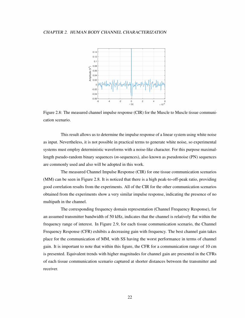
Figure 2.8: The measured channel impulse response (CIR) for the Muscle to Muscle tissue communi-

cation scenario.

This result allows us to determine the impulse response of a linear system using white noise

as input. Nevertheless, it is not possible in practical terms to generate white noise, so experimental

systems must employ deterministic waveforms with a noise-like character. For this purpose maximal-

length pseudo-random binary sequences (m-sequences), also known as pseudonoise (PN) sequences

are commonly used and also will be adopted in this work.

The measured Channel Impulse Response (CIR) for one tissue communication scenarios

(MM) can be seen in Figure 2.8. It is noticed that there is a high peak-to-off-peak ratio, providing

good correlation results from the experiments. All of the CIR for the other communication scenarios

obtained from the experiments show a very similar impulse response, indicating the presence of no

multipath in the channel.

The corresponding frequency domain representation (Channel Frequency Response), for

an assumed transmitter bandwidth of 50 kHz, indicates that the channel is relatively flat within the

frequency range of interest. In Figure 2.9, for each tissue communication scenario, the Channel

Frequency Response (CFR) exhibits a decreasing gain with frequency. The best channel gain takes

place for the communication of MM, with SS having the worst performance in terms of channel

gain. It is important to note that within this figure, the CFR for a communication range of 10 cm

is presented. Equivalent trends with higher magnitudes for channel gain are presented in the CFRs

of each tissue communication scenario captured at shorter distances between the transmitter and

receiver.

22


Frequency (Hz) ×105

1 2 3 4 5 6 7 8 9 10

Ma

gn

itud

e (

dB

)

-40

-35

-30

-25

-20

-15

-10

-5

0

SS

MM

MS

SM

Figure 2.9: Channel Frequency Response (CFR) for all tissue communication scenarios for d = 10

cm.

2.2.1.1 Noise Analysis and Capacity Estimation

Another set of measurements were taken in the porcine tissue for the assessment of the

noise characteristics, including probability distribution and spectral power.

Noise Characteristics The results show that the noise’s probability density function is a good

approximation of a normal distribution. The frequency analysis presents a fairly flat power spectral

density with a noise power spectral density dependent on the layer of tissue, and is summarized in

Table 2.2.

Table 2.2: Noise power spectral density

Medium N0

MM, SM �107.0dBm

MS, MS �105.5dBm

Based on these results, the channel is considered a zero-mean Additive White Gaussian

Noise (AWGN) and treated as such for channel capacity estimation.

Channel Capacity For an AWGN channel we employ the well known Shannon-Hartley formula

given by (2.15) to make an estimate of the maximum achievable capacity of the system. The

calculations are made using the measured received power PRX for several locations and for a signal

covering the whole 900 kHz bandwidth.

23


C = BW · log2✓1 +

PRX

N0 ·BW

◆(2.15)

Figure 2.10 shows the results for different Tx–Rx combinations whereas Figure 2.11

presents one comparison example of the channel capacity estimation from the experimental data

and results from the 2-port circuit model, presented for a center frequency of 100 kHz and the noise

levels mentioned previously. Results indicate a similar range of values for capacity estimation, even

in the presence of the differences among tissue exposure to the environment that was not modeled in

[5].

5 10 150

1

2

3

4

5

·106

Distance (cm)

Cha

nnel

Cap

acity

(bps

)

MMMSSMSS

Figure 2.10: Channel capacity estimate for different layers and distances, under the assumption of an

AWGN channel.

MM MS SM SS

Channel C

apaci

ty (

bps)

×106

0

1

2

3

4

5

6

7

8

2-Port Circuit Model

Experimental Data

Figure 2.11: Experimental channel capacity estimate comparison with 2-port circuit model by [5] for

d = 10 cm and a center frequency of 100 kHz.

24


2.3 Thermal Analysis

One of the main concerns in using any wireless communication method on or within the

body is the inherent heating of the tissue due to the applied energy. Galvanic coupling has to be

necessarily constrained in terms of transmission power to stay under safe conditions, as it generates

significant currents in the tissue. Nevertheless, the maximum limit of 1 mW is well below the

international regulation on electromagnetic fields on the human body.

Our purpose in this section is two-fold: a) evaluate the change in temperature with a

transmitter coupled on skin, and b) compare the effect of the two modulation paradigms (continuous

wave and pulse-based) to assess which one prevents heating the most.

The underlying assumptions are the following: a one-dimensional description of the

temperature in a semi-infinite tissue layer is enough to provide an estimate of the temperature

distribution and a comparison of the different power inputs (the modulation schemes.) For this

analysis we follow the approach of [29].

The most popular approach to heat propagation in biological tissue is based on the study of

Pennes [30]. He provided the so called “bioheat transfer equation,” a three-dimensional description

of the temperature depending on physical parameters of the tissue, blood, core temperature, and

surrounding temperature. The generalized one-dimensional bioheat transfer equation is given by:

⇢c@T

@t= k

@2T

@x2+ !b⇢bcb (Ta � T ) +Qm +Qr(x, t) (2.16)

All variables are detailed in Table 2.3. The key difference here with respect to the standard

heat transfer is that the factor !b⇢bcb (Ta � T ) takes into account the “perfusion” of the blood,

that is, the effect of the blood flow on the temperature distribution, modeled as “volumetrically

distributed heat sinks or sources” [29]. The blood perfusion rate term !b is a frequency with units 1/s

or equivalently mL/(s mL).

The derivation of the solution for this problem is developed in more detail in [29]. We are

presenting here the results. The solution to equation (2.16) is given as

T (x, t) = T0(x) +W (x, t) exp

✓�!b⇢bcb

⇢ct

◆(2.17)

Overall, equation (2.17) provides the value of the temperature at a linear distance x

and at time t, as a function of T0(x), the initial temperature at t = 0, W (x, t), which is a term

that groups the influence of a spatial heat source, tissue parameters and boundary conditions, and

25


Table 2.3: Tissue and Blood Thermal Parameters

Symbol Name Units Value in Simulation

Ae Electrodes contact area m23⇥ 10

�4

c Specific heat of tissue J/(kg �C) 4200

cb Specific heat of blood J/(kg �C) 4200

h0 Heat convection coefficient W/(m2 �C) 10

hf Heat convection coefficient W/(m2 �C) 100

k Thermal conductivity of tissue W/(m �C) 4200

L Distance between skin surface

and body core

m 3⇥ 10

�2

P0(t) Spatial heating power flux at skin

surface

W/m2 Eq. (2.26)

Qm Metabolic rate of tissue W/m333 800

Qr(x, t) Spatial heating W/m3 Eq. (2.25)

t, ⌧ Time s —

T (t) Tissue temperature �C Eq. (2.17)

Ta Artery temperature �C 37

Tc Body core temperature �C 37

Tf Fluid temperature �C 25

W (x, t) Transformed temperature �C Eq. (2.22)

x, ⇠ Spatial coordinate m —

↵ Thermal diffusivity of tissue m2/s 1.1905⇥ 10

�7

⌘ Scattering coefficient 1/m 200

!b Blood perfusion 1/s 0.5⇥ 10

�3

⇢ Density of tissue kg/m31000

⇢b Density of blood kg/m31000

26


exp (�(!b⇢bcb)/(⇢c)t), an exponential factor that vanishes to reach thermal equilibrium as t ! 1and depends on the physical properties of tissue and blood.

As in (2.17), the higher the blood perfusion rate, the faster the temperature falls off as

t ! 1 (notice that for the simulation ⇢b = ⇢ and cb = c therefore they cancel out and the exponential

term depends solely on !b.

The initial basal temperature is given by

T0(x) =Ta +Qm

!b⇢bcb

+

⇣Tc � Ta � Q

m

!b

⇢b

cb

⌘·hp

A cosh

⇣pAx

⌘+

h0k sinh

⇣pAx

⌘i

pA cosh

⇣pAL

⌘+

h0k sinh

⇣pAL

⌘

+

h0k

⇣Tf � Ta � Q

m

!b

⇢b

cb

⌘· sinh

⇣pA(L� x)

⌘

pA cosh

⇣pAL

⌘+

h0k sinh

⇣pAL

⌘

(2.18)

dT0(x)

dx=

⇣Tc � Ta � Q

m

!b

⇢b

cb

⌘·hA sinh

⇣pAx

⌘+

pAh0

k cosh

⇣pAx

⌘i

pA cosh

⇣pAL

⌘+

h0k sinh

⇣pAL

⌘

+

h0k

⇣Tf � Ta � Q

m

!b

⇢b

cb

⌘·�

pA cosh

⇣pA(L� x)

⌘

pA cosh

⇣pAL

⌘+

h0k sinh

⇣pAL

⌘

(2.19)

The Green equation is used to solve the differential equation, and its expression is

G1(x, t; ⇠, ⌧) =2

L

1X

m=1

e�↵�2m

(t�⌧)cos(�mx) cos(�m⇠)H(t� ⌧) (2.20)

where,

�m =

2m� 1

2L⇡, with m = 1, 2, 3, . . . (2.21)

The solution for the transformed temperature W (x, t) is

W (x, t) =↵

k

Z t

0G1(x, t; ⇠, ⌧)|⇠=0 g1(⌧) d⌧

+

Z t

0d⌧

Z L

0G1(x, t; ⇠, ⌧)

Qr(⇠, ⌧)

⇢cexp

✓!b⇢bcb⇢c

⌧

◆d⇠

(2.22)

in which

27


g1(t) =

k

dT0(x)

dx

��x=0

+ f1(t)

�exp

✓!b⇢bcb⇢c

t

◆H(t) (2.23)

We will adopt a surface adiabatic condition and spatial heating, where the heat flux is given

by

qr(x, t) = P0(t) exp(�⌘x) (2.24)

and the spatial heating can be obtained as

Qr(x, t) = �@qr@x

= ⌘P0(t) exp(�⌘x) (2.25)

for a power source given by

P0(t) =s2(t)/RTX

Ac(2.26)

In this last term is where our transmission signals reside. P0(t) is the time-dependent

heating power on skin surface.

28

Chapter 3

Modulation Techniques for GalvanicCoupling

Due to its novelty, there are not clearly defined modulation schemes for the physical layer

of Intrabody Communications in any of its forms (galvanic or capacitive coupling, ultrasound.)

Some works have focused in quadrature phase-shift keying (QPSK) [26][31], differential binary

phase-shift-keying (DBPSK) [8], on-off-keying (OOK) and direct sequence spread spectrum (DSSS)

[2][32], frequency-shift keying (FSK) [33], continuous phase frequency shift keying (CPFSK) [3],

and pulse position modulation (PPM) [34][6].

For the present work we will evaluate six different modulation schemes, divided in two

categories: Continuous Wave Modulation (CWM) schemes, as explained in Section 3.1 and Pulse-

Based Modulation (PBM) schemes, detailed in Section 3.2. The purpose is to compare them as

two different paradigms to assess the performance of each one and examine their advantages and

disadvantages.

In this chapter, first a description of the modulation schemes is made, including the

selection of the waveform for PBM.

A Note On Orthogonality A set of base functions of an N -dimensional space is called orthogonal

if the following relation holds:

Z t2

t1

�n(t)�⇤m(t) dt =

8><

>:

0 n 6= m

Kn n = m(3.1)

29

CHAPTER 3. MODULATION TECHNIQUES FOR GALVANIC COUPLING

This operation is known as inner product of two functions and is usually denoted as

h�n(t),�m(t)i [35]. Also, if

Kn =

Z t2

t1

|�n(t)|2 dt = 1 for all n (3.2)

then they are called orthonormal. This concept, although simple in appearence, is a

fundamental tool for modulation and demodulation of signals, particularly in correlation-based

coherent reception for pulse-based modulation.

3.1 Continuous Wave Modulation

Carrier, or continuous wave, modulation is a bidimensional modulation with two orthogo-

nal base functions (modulators) given by (3.3),

�1(t) =q

2T cos(2⇡fct)

�2(t) =q

2T sin(2⇡fct)

(3.3)

whereq

2T is a normalization factor and T is the integration period. According to the inner

product operation given in (3.2) they are orthonormal, so that

Z T

0|�n(t))|2 dt = 1 for n = 1, 2

.

The function �1(t) is called In phase and �2(t) in Quadrature, therefore the signal s(t) in

this bidimensional space is known as IQ modulation [36] and is written as

s(t) = sI cos(2⇡fct) + sQ sin(2⇡fct) (3.4)

where sI and sQ are the in-phase and the quadrature components of the modulated signal,

respectively.

More generally, the function g(t) represents the filter of the signal, chosen to adjust the

desired spectral properties, therefore

si(t) = si1g(t) cos(2⇡fct) + si2g(t) sin(2⇡fct) (3.5)

30


a0, a1, a2, . . .QAM/PSK

Mapper

TX Filter

g(t)

TX Filter

g(t)

⇠Local

Oscillator

90

�Phase

Shift

⇥

⇥

+

In Phase

Quadrature

sI

sQ

cos(2⇡fct)

sin(2⇡fct)

s(t)

TX

Figure 3.1: IQ modulator diagram, showing the optional (but desirable or required) transmission

filter.

where the components sij correspond to the i-th symbol of one of the j = 2 base functions,

�1,2(t). In this work, a raised cosine filter is applied.

The set si = {s1, s2, s3, . . . , sm} is known as constellation points and their values are

given as complex numbers. A simplified, generic block diagram of a the transmitter of an IQ

modulation system is shown in Figure 3.1 and the receiver in Figure 3.2.

Quadrature Amplitude Modulation and Phase Shift Keying Both QAM and PSK are part of

the general group of IQ modulation schemes. Their transmission and reception structural diagram

is essentially the same, and the main difference lies within the mapping of the symbols, with

corresponding constellation diagrams shown in Figures 3.3a and 3.3b.

Simulation and Experimental Diagram The components of the system that is simulated and

experimentally tested is shown in Figure 3.4. Both the convolutional encoding and the filtering are

optional steps.

3.2 Pulse-Based Modulation

Pulse-based modulation or simply pulse modulation (also known as Impulse Radio in

the context of ultrawideband) consists in the transmission of very short pulses with high energy

31


a0, a1, a2, . . .QAM/PSK

Mapper

⇥

⇥

LPF

LPF

RX Filter

g⇤(t)

RX Filter

g⇤(t)

⇠ Local

Oscillator

90

� Phase

Shift

sI In Phase

sQQuadrature

cos(2⇡fct)

sin(2⇡fct)

r(t)

RX

Figure 3.2: IQ demodulator diagram, with the matched filter g⇤(t).

I

Q0000 0100 1100 1000

0001 0101 1101 1001

0011 0111 1111 1011

0010 0110 1110 1010

(a) Rectangular 16-QAM

I

Q

011

010

110

111

101

100

000

001

(b) 8-PSK with zero phase shift

Figure 3.3: Constellation diagrams with Gray coding: each adjacent symbol differs by only one bit.

32


Data

Source

Convolutional

Encoder

Baseband

Modulation

TX Filter /

Upsampling

Passband

ModulationAFE

Channel

Received

Data

Convolutional

Decoder

Baseband

Demodulation

RX Filter /

Downsampling

Passband

DemodulationAFE

Continuous-Wave Modulation Transmitter

Continuous-Wave Modulation ReceiverFigure 3.4: The diagram shows optional steps in dashed blocks. AFE stands for Analog Front End.

concentration in the interval Tp, yielding very high bandwidths. The data can be conveyed in the

amplitude, phase, position, or shape of the pulses, plus the combination of them for higher order

schemes.

Intrabody communications use low frequencies (below or about 1 MHz), even though, the

pulse modulation hereby described fits part of the definition for Ultrawideband (UWB), as given by

the FCC Part 15 Rule. An ultrawideband pulse is any signal for which [37]:

Bf � 0.2 (3.6)

or

BW � 500 MHz (3.7)

where Bf is the “fractional bandwidth,” defined as:

Bf =

BW

fc=

(fH � fL)

(fH + fL)/2(3.8)

where fH and fL are the upper and lower cutoff frequencies of the transmission band of

�10 dB, BW is the bandwidth and fc the central frequency.

Our system has a bandwidth of 900 kHz and a center frequency of 550 kHz, then using 3.8

33


Data

Source

Convolutional

Encoder

Baseband

ModulationAFE

Channel

Received

Data

Convolutional

Decoder

Baseband

DemodulationAFE

Transmitter

ReceiverFigure 3.5: Pulse-based modulation general block diagram

Bf =

BW

fc=

900

550

= 1.636 � 0.2

An important features is that a shift in center frequency can be obtained by pulse shaping.

The general structure for the transmission and reception is shown in Figure 3.5.

Features Borrowing from the analysis already performed in the context of radiofrequency ultraw-

ideband, we list here some of the main characteristics and advantages of pulse modulation.

• An important feature is that when N orthogonal pulses are used, it is possible to create an

N -dimensional space, usfeul for higher order modulation schemes.

• It is carrier-less (baseband) and therefore a mixer is not required, yielding simpler and cheaper

transmitters.

• No additional filtering required to fit a spectral mask (once the pulses have been “fine tuned”

to the desired frequencies.)

• For some PBM schemes, unlike QAM, the amplitude of the received signal is not important

therefore no adjustment is necessary.

• In a multipath environment (not in the case of IBC) it is possible to apply techniques like Rake

receivers thanks to its fine time resolution.

34


• For the same reason above, it is possible to perform ranging strategies.

• New multiple access techniques have been applied, including Time-Hopping (TH).

• The “hard limit” of the symbol rate of a PBM scheme is the inverse of the pulse duration,

because it is impossible to “shrink it” anymore. Even though, it is possible to achieve higher

bit rates if the scheme is M -ary. For example, for BPM and pulses of Tp = 2µs the maximum

bit rate is R = 1/Tp = 500 kbps, whereas for 4-PSM the maximum bit rate is twice that value.

3.2.1 Pulse-Based Modulation Schemes

There are both binary and M -ary modulation schemes. In this work we will introduce new

schemes with promising application in intrabody communications.

The most common modulation schemes are explained below [37][38]. Let s(t) be the

transmission signal, ai the amplitude mapped to the i-th symbol, p(t) the pulse, and Ts the period of

the symbol.

Pulse Amplitude Modulation PAM is described by

s(t) =1X

i=�1aip (t� iTs) (3.9)

On-Off Keying OOK is the simplest PAM modulation scheme, with one bit per symbol, for which

s(t) =

1X

i=�1aip (t� iTs) , with ai = {1, 0} (3.10)

Bi-Phase Modulation BPM is another binary PAM variation and can be expressed as

s(t) =

1X

i=�1aip (t� iTs) , with ai = {1,�1} (3.11)

0 1

Figure 3.6: BPM

35


Pulse Position Modulation PPM encodes the information in �shiftTp, and �shift is known as

“modulation index.” M -ary modulation can be achieved although it is usually binary. It smooths the

“spectral lines,” that are a consequence of the periodic pulse transmission of other schemes.

s(t) =1X

i=�1p (t� iTs + �shiftTp) , with 0 �shift < 1 (3.12)

0 1

�shiftTp

Figure 3.7: Binary PPM

Pulse Shape Modulation PSM employs different orthogonal pulse waveforms. If

s(t) =

1X

i=�1pi,m (t� iTs) (3.13)

then pi,m(t) is the m-th waveform of the i-th symbol.

0 1

Figure 3.8: Binary PSM

For an M -ary modulation scheme, M pulses are required. Table 3.1 shows the mapping of

4-PSM for a set of M = 4 orthogonal waveforms {�m(t)}.

Soft Spectrum Keying In SSK, every pulse is considered as a bit itself, where the information bits

{0, 1} are conveyed in its sign or amplitude. For an M -ary modulation scheme, k = log2M pulses

are required1.1Thus using the pulses more efficiently than PSM, in terms of bits per pulses.

36


Table 3.1: 4-PSM Modulation Mapping

Waveform pi,m(t) Symbol

�i1(t) 00

�i2(t) 01

�i3(t) 10

�i4(t) 11

s(t) =

1X

i=�1

kX

j=1

aijpj (t� iTs) (3.14)

where aij is the j-th bit of the i-th symbol and pj(t) is the j-th orthogonal waveform.

00 01 10 11

Figure 3.9: SSK with OOK inner modulation

Table 3.2 shows the mapping of the pulses for 8-SSK, with a set of k = 3 orthogonal

waveforms {�k(t)}, and Figure 3.10 and 3.11 show the structure of the transmitter and receiver,

respectively.

37


Table 3.2: 8-SSK Modulation Assignment

Sign of Waveform

�1(t) �2(t) �3(t) Symbol

+ + + 000

+ + � 001

+ � + 010

+ � � 011

� + + 100

� + � 101

� � + 110

� � � 111

a1, a2, a3, . . .

ai = {�1, 1}

Serial /

Parallel⇥

⇥

⇥

+

�1(t)

�2(t)

�3(t)

a1

a2

a3

s(t)

TX

Figure 3.10: Transmitter structure of the 8-SSK modulation

Reception of PBM Signals The received signal r(t) is given by

r(t) = Acs(t) + n(t) (3.15)

where Ac is an attenuation factor and n(t) is white Gaussian noise. To “detect” a pulse

38


from among a set of orthogonal waveforms we should perform the inner product presented in (3.1),

h�n(t),�m(t)i. Assuming perfect synchronization, the correlation with an orthogonal pulse template

will be zero, and any other value (positive or negative) otherwise.

Let us use 8-SSK as an example. Let the following bits with antipodal encoding2

{a1, a2, a3} = {1,�1, 1} be one symbol of the transmission signal, as

s(t) = a1�1(t) + a2�2(t) + a3�3(t) = �1(t)� �2(t) + �3(t)

In the correlation in the first branch in Figure 3.11 the result is

a1(t) = hr(t),�1(t)i

= hAc(�1(t)� �2(t) + �3(t)) + n(t),�1(t)i

= hAc�1(t),�1(t)i+ h�Ac�2(t),�1(t)i+ hAc�3(t)),�1(t)i+ hn(t),�1(t)i

= Ac + n(t)

The symbol decision is simple and just evaluates whether ai(t) is greater or less than zero.

a1, a2, a3, . . .Parallel

/ Serial> 0

> 0

> 0

Z T

0

Z T

0

Z T

0

⇥

⇥

⇥

�1(t)

�2(t)

�3(t)

a1(t)

a2(t)

a3(t)

a1

a2

a3

r(t)

RX

Correlator Symbol Decision

Figure 3.11: Receiver structure of the 8-SSK modulation

2What in this context is known as BPM inner modulation.

39


Ts 2Ts 3Ts 4Ts 5Ts

·10�5

�20

�10

0

10

20

10 01 11 10 00

Volta

ge(m

V)

(a) 4-PSM: One waveform per symbol

Ts 2Ts 3Ts 4Ts 5Ts

·10�5

�10

0

10

1000 1110 1111 1010 1100

Volta

ge(m

V)

(b) 16-SSK: The sum of four orthogonal waveforms per symbol

Figure 3.12: These are the first five symbols of two pulse-based modulation schemes.

Figure 3.12 shows two examples of the first symbols of PBM schemes.

3.2.2 Waveform Selection

The selection of the waveform for PBM will be considered here due to its importance for

the modulation schemes. In particular, we are interested in a bandlimited pulse with high energy

concentration in a given time interval, but also it is desirable to have an orthogonal set of pulses

that lead to new modulation schemes such as PSM and SSK, described above. Two waveforms

are considered for this work: Gaussian derivatives and prolate spheroidal wave functions (PSWF.)

Previous works [34] have used rectangular pulses, regardless of the bandwidth occupancy and the

40


modulation capabilities of other sets. The utilization of PSWF pulses for IBC has not been reported.

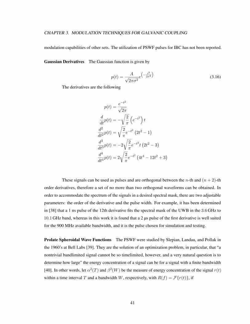
Gaussian Derivatives The Gaussian function is given by

p(t) =Ap2⇡�2

e

⇣� t

2

2�2

⌘

(3.16)

The derivatives are the following

p(t) =e�t2

p2⇡

d

dtp(t) = �

r2

⇡

⇣e�t2

⌘t

d2

dt2p(t) =

r2

⇡e�t2

�2t2 � 1

�

d3

dt3p(t) = �2

r2

⇡e�t2t

�2t2 � 3

�

d4

dt4p(t) = 2

r2

⇡e�t2

�4t4 � 12t2 + 3

�

These signals can be used as pulses and are orthogonal between the n-th and (n+ 2)-th

order derivatives, therefore a set of no more than two orthogonal waveforms can be obtained. In

order to accommodate the spectrum of the signals in a desired spectral mask, there are two adjustable

parameters: the order of the derivative and the pulse width. For example, it has been determined

in [38] that a 1 ns pulse of the 12th derivative fits the spectral mask of the UWB in the 3.6GHz to

10.1GHz band, whereas in this work it is found that a 2 µs pulse of the first derivative is well suited

for the 900 MHz available bandwidth, and it is the pulse chosen for simulation and testing.

Prolate Spheroidal Wave Functions The PSWF were studied by Slepian, Landau, and Pollak in

the 1960’s at Bell Labs [39]. They are the solution of an optimization problem, in particular, that “a

nontrivial bandlimited signal cannot be so timelimited, however, and a very natural question is to

determine how large” the energy concentration of a signal can be for a signal with a finite bandwidth

[40]. In other words, let ↵2(T ) and �2(W ) be the measure of energy concentration of the signal r(t)

within a time interval T and a bandwidth W , respectively, with R(f) = F{r(t)}, if

41


↵2(T ) =

R T/2�T/2 r

2(t) dt

R1�1 r2(t) dt

(3.17)

and

�2(W ) =

RW�W R2

(f) dfR1�1R2

(f) df(3.18)

then the question is how big can ↵2(T ) be for a band-limited signal r(t). The answer to

this optimization problem is the set of prolate spheroidal functions, n(t), having the following

properties:

• n(t) has even and odd symmetry with n.

• n(t) ⇠ knsin ctt , when t ! 1.

•R 1�1 e

j2⇡st n(t) dt = ↵n n(2⇡s/c), i.e., its Fourier transform has the same shape.

• Bandwidth is c/2⇡.

• The pulses are doubly orthogonal.

• Bandwidth and pulse width can be simultaneously controlled and are constant for all orders.

• Zero DC component and baseband.

There is no closed form of the signals, so it is necessary then to adopt a numerical

approximation. The method used in this work is the one given by [41]. With such procedure we can

obtain a pulse like the one in Figure 3.13a with a spectral mask depicted in Figure 3.13b, fitted for

UWB. The flexibility of the PSWF and this algorithm allows us to easily adapt the pulse to our needs

in the bandwidth of 100 kHz to 1000 kHz. In fact, the pulse width, and the lower and upper limit of

the frequency band can be explicitly indicated.

3.3 Simulations and Experimental Testing

A platform for testing the modulation schemes was created in Matlab for both continu-

ous wave and pulse-based modulation. Regarding PBM, the function pulsegen generates both

Gaussian and PSWF pulses as described in Section 3.2, fitting in the allowed bandwidth. The

42


0 0.2 0.4 0.6 0.8 1

�0.1

�0.05

0

0.05

Time [ns]

Am

plitu

de

(a) Time Domain

0 5 10 15 20 25

�300

�250

�200

�150

�100

Frequency [MHz]

Pow

er/F

requ

ency

[dB

/Hz]

Power Spectral Density

(b) Frequency Response

Figure 3.13: PSWF pulse for the UWB spectral mask.

43


Table 3.3: This table shows a summary of the main parameters of the pulse-based modulation schemes

evaluated in the simulations. The pulse width for all is Tp = 5 µs, which implies a maximum symbol

rate of 200 ksps.

ModulationOrder

M

Bits per

Symbol

k

Required

PulsesWaveform

Bandwidth

BW

(kHz)

Max Bit Rate

Rbit,max

(kbps)

BPM 2 1 k Gaussian 587 200

PPM 2 1 k Gaussian 614 200

PSM 2 1 M Gaussian 611 200

PSM 4 2 M PSWF 795 400

SSK 4 2 k PSWF 620 400

SSK 8 3 k PSWF 687 600

SSK 16 4 k PSWF 759 900

duration is fixed and set to 5 µs. Then pulsemod and pulsedemod perform the modulation and

demodulation of the signals. Optionally, convolutional encoding and Viterbi decoding can be enabled

for both.

Figure 3.14 and 3.15 illustrate the structure of the programs. In the channel, for a simulation

the signal is attenuated and noise is added according with the results of the channel characterization

in Chapter 2.

A Note on the Simulations Several simulations are made, for up to 10

6 bits and encompassing all

modulation schemes. The set of simulations is made with an AWGN channel based on the analysis

in Chapter 2, in which the parameters for attenuation and noise power spectral density are obtained.

These results are a benchmark of the achievable bit error rates.

In the following sections, an analysis of the characteristics of each modulation is made,

and the results of the simulations are compared to finally provide a recommendation for this system.

Unless otherwise noted, all simulations were made for the following parameters:

• Medium: skin-to-skin (SS)

• Distance between transmitter and receiver: 15 cm

• Symbol rate: 150 kbps

44


Parameter Selection

Data Bits

PSK or QAM

Modulation Object

Raised Cosine

Tx Filter Object

Passband

Modulation

CHANNEL

Simulation or Experiment

Passband

Demodulation

Raised Cosine

Rx Filter Object

PSK or QAM

Demodulation Object

Received BitsBER

Analysis

Figure 3.14: Structure of the program in Matlab for CWM

Parameter Selection

Data Bits

pulsemodpulsegen

CHANNEL

Simulation or Experiment

pulsedemodpulsegen

Received Bits

BER

Analysis

Figure 3.15: Structure of the program in Matlab for PBM

45


• CWM bandwidth: 200 kHz (approximately)

• Number of bits of simulation: 106

Regarding the comparison of the two classes of modulation schemes:

Schemes for M = 2 The only binary modulation in CWM performs better than (or equal to) the

PBM schemes.

PTX

(dBm)-40 -38 -36 -34 -32 -30 -28 -26 -24 -22 -20

BE

R

10-5

10-4

10-3

10-2

10-1

100

BPSKBPMPPM2-PSM

Figure 3.16: Simulations with M = 2.

Schemes for M = 4 For M = 4, CWM still outperforms PBM.

46


PTX

(dBm)-40 -38 -36 -34 -32 -30 -28 -26 -24 -22 -20

BE

R

10-6

10-5

10-4

10-3

10-2

10-1

100

4-PSM4-SSKQPSK


Schemes for M = 8 There is an interesting change in M = 8, for which PBM shows better

performance. This is analyzed in more detail in the Power Efficiency section below.

PTX

(dBm)-40 -35 -30 -25 -20 -15 -10

BE

R

10-5

10-4

10-3

10-2

10-1

100

8-PSK8-QAM8-SSK


47


Schemes for M = 16 Here again PBM presents better BER. As in M = 8, this performance

comes at a price, especially at the receiver where more correlators are required to demodulate the

signal.

PTX

(dBm)-40 -35 -30 -25 -20 -15 -10 -5

BE

R

10-5

10-4

10-3

10-2

10-1

100

16-QAM16-SSK16-PSK


Varying Distances As expected, with increased distance, worse performance, in both cases. For

d = 5 cm, no errors were registered.

48


PTX

(dBm)-40 -38 -36 -34 -32 -30 -28 -26 -24 -22 -20

Bit

Err

or

Ra

te

10-5

10-4

10-3

10-2

10-1

100

QPSK d = 15 cmQPSK d = 10 cm4-SSK d = 15 cm4-SSK d = 10 cm

Figure 3.20: Two modulation examples for different distances.

Different Channels The channel plays a heavy role in performance. Whether the signal is going

through or across tissue will change the gain and thus the power at the receiver.

PTX

(dBm)-40 -38 -36 -34 -32 -30 -28 -26 -24 -22 -20

Bit

Err

or

Ra

te

10-6

10-5

10-4

10-3

10-2

10-1

100

QPSK MMQPSK MSQPSK SMQPSK SS

Figure 3.21: QPSK for different channels.

49


PTX

(dBm)-40 -38 -36 -34 -32 -30 -28 -26 -24 -22 -20

Bit

Err

or

Ra

te

10-6

10-5

10-4

10-3

10-2

10-1

100

4-SSK MM4-SSK MS4-SSK SM4-SSK SS

Figure 3.22: 4-SSK for different channels.

Different Bit Rates The higher the bit rate, the higher the bit error rate.

PTX

(dBm)-40 -38 -36 -34 -32 -30 -28 -26 -24 -22 -20

Bit

Err

or

Ra

te

10-6

10-5

10-4

10-3

10-2

10-1

100

QPSK 200 kbpsQPSK 300 kbps4-SSK 300 kbps4-SSK 200 kbps

Figure 3.23: Different bit rates.

All Pulse-Based Schemes at Same Symbol Rate The ranking of all PBM schemes is shown here.

50


PTX

(dBm)-40 -38 -36 -34 -32 -30 -28 -26 -24 -22 -20

BE

R

10-5

10-4

10-3

10-2

10-1

100

BPMPPM2-PSM4-PSM4-SSK8-SSK16-SSK

Figure 3.24: All PBM schemes.

Decrease in Performance as M Increases As noted before, there is a steeper degradation of the

performance of CWM as the order of the modulation increases.

PTX

(dBm)-40 -35 -30 -25 -20 -15 -10

Bit

Err

or

Ra

te

10-5

10-4

10-3

10-2

10-1

100

4-PSK4-SSK8-SSK16-SSK8-PSK16-PSK

Figure 3.25: Performance with respect to M .

51


3.4 Criteria for Selection of the Modulation Scheme

System Complexity The absence of a mixer and a filter in the transmitter of the pulse modulator

makes here an important difference. In Chapter 4 we analyze a set of sensors with only transmission

capabilities, that reduce the power consumption and hardware considerably.

Bandwidth Efficiency In this concern, CWM performs better, as for this set of simulations the

bandwidth was of 200 kHz versus the 700 kHz of average of the PBM, for the same symbol rate in

all cases.

Power Efficiency For power efficiency, there is an interesting finding: as the order of the modu-

lation, M , increases, the CWM schemes see a serious degradation of its performance, whereas for

PBM it is milder. This can be seen clearly in Figure 3.25.

Conclusions

• Although not completely fair comparison (as PBM has wider bandwidth), an initial assessment

of the two modulation categories show that, if only hardware is considered, PBM provides

better value.

• BPSK and BPM, as well as QPSK and 4-SSK3 have exactly the same performance.

3Notice that BPM and 2-SSK are completely equivalent.

52

Chapter 4

Elements of Intrabody Network Design

The practical implementation of a Galvanic Coupled Intrabody Communications (GC-

IBC) network requires solving important challenges regarding synchronization and multiple access

schemes. The former is critical if an impulse modulation method is applied, whereas the latter is a

very natural challenge that arises in a myriad of possible applications, for example, when a population

of sensors reach a single data sink.

We will focus our efforts in the description of a synchronization method and a Medium

Access Control (MAC) protocol for the Pulse-Based Modulation (PBM) schemes described in Chapter

3. Similar issues have been addressed previously for Impulse Radio Ultrawideband (IR-UWB) and

we adopt some of its techniques to our own needs.

Scenario of a Sensor Network In the following sections we will describe synchronization and

multiple access strategies for an envisioned application with multiple satellite transmitters and a

single receiver, as in Figure 4.1, and with an operation regime outlined in Table 4.1. The description

is given as follows:

Satellite Transmitters They are low power, low complexity, sensor-transmitter units, possibly many

and distributed over a region of the body. There is a single hop between each one and the

central receiver. They have no reception capabilities in order to save energy and hardware. The

sensors might be different, although there also might be some redundancy in the information

they send.

Central Receiver It is in charge of the synchronization of the received signals and capable to receive

data from multiple sensors simultaneously. It presents higher complexity, with transmission/re-

53

CHAPTER 4. ELEMENTS OF INTRABODY NETWORK DESIGN

T1

T2 T3

T4

T5

T6T7

T8 T9

R0

GC-IBC Link

Figure 4.1: The scenario of a network of sensors communicating to a single receiver in an uncoordi-

nated, unidirectional star topology.

ception capabilities.

4.1 Synchronization

In a PBM regime, it is critical to have good synchronization. As in IR-UWB, “even a slight

misalignment can severely degrade the system performance (. . . ) especially if correlation based

coherent receiver is opted” [42], as is the case in our system.

One category of methods to attain synchrony in an impulsive signal uses the data pulses

themselves to detect the timing offset, ⌧ . The most well known are: Timing with Dirty Template

(TDT), Timing with Code Matching (TCM), and Timing with Energy Detection (TED.) The reader

is referred to the work by Akbar [42] and references therein.

A second class of synchronization methods uses dedicated synchronization headers in the

packet along with (possibly) special circuitry for the detection of the offset. The preferred strategy in

this work will be to introduce a special header in every sent packet. This is a reasonable alternative

because of the low data rate and bursty nature of the transmission, therefore it is not crucial to “save

time” by doing synchronization “on the fly.” We will follow closely the design proposed by Di

Benedetto [43], where a synchronization branch is attached to the receiver, as shown in Figure 4.4.

Synchronization Process A series of pulses with appropriate auto-correlation, noise-like properties

is sent to activate the Synchronization Branch of the receiver’s front end. The packet format is given

in Figure 4.2.

54


Table 4.1: Features of a proposed network for analysis.

Central Unit Sensors

Communication Reception from sensors and transmis-

sion to other neighbor receivers or an

external data sink.

Only transmission.

Behavior Continuously senses for new trans-

missions from the network and syn-

chronizes with new incoming packets,

but does not send any acknowledge-

ment. Once a “connection” with a

new packet is established, it can de-

tect other incoming packets simultane-

ously.

The sensor is continuously recording

information, nevertheless, the trans-

mission only takes place at a prede-

fined schedule in different regimes (de-

pending on the application) and the

transmission hardware is sleeping at

any other moment.

Regimes A. Continuous detection. A. Normal operation: constant rate

of transmissions, B. Special operation:

when a particular condition is detected

and thus the sensor data requires an

increased transmission rate.

Synchronization Synchronizes with every incoming

packet from different transmitters.

Uncoordinated. They send a synchro-

nization header on each packet to ac-

count for clock drift of devices sub-

ject to changes in temperature, with

not very sophisticated clocks, and with

very long sleeping periods.

Power Higher demand. Minimal.

MAC The receiver knows the multiple ac-

cess code of the associated devices and

after synchronization it matches the

code of the transmitter for receiving a

packet.

Each terminal has a unique code for

transmitting. This multiple access se-

quence is fixed (“hard coded”) and is

used in every transmission.

55


Synchronization

HeaderPreamble Payload

Figure 4.2: Packet format.

The segment of the packet with the synchronization header from the transmitter is called

here sTsync(t). This signal will be defined as a bi-phase-modulated m-sequence of length Nm�seq. The

reason to choose this signal is due to its noise-like properties, namely the adequate auto-correlation

properties (see equation 2.12.) Figure 4.3 presents the auto-correlation function of an example of

such signals.

�5 �4 �3 �2 �1 0 1 2 3 4 5

·10�4

�0.5

0

0.5

1

Delay ⌧ (s)

Nor

mal

ized

Aut

ocor

rela

tion Pulse Bi-Phase Modulated PN Sequence

Figure 4.3: The auto-correlation of the synchronization header shows a high peak to side lobes ratio.

In the implementation, though, the receiver has a copy of it, sRsync(t), and a cross-correlationˆRss(⌧) , sTsync(t) ? s

Rsync(t) is applied once the incoming packet is detected. When the two signals

are “aligned,” a peak is generated and detected, so that it triggers the synchronized timing for this

packet.

The peak detector of the correlation function in the Synchronization Branch will start the

timing mechanism, now with a known offset timing, ⌧ .

Identification of the Transmitter Each transmitter follows a certain multiple access scheme to

send the data while sharing the medium. For the receiver to demodulate the signal, it has to necessarily

know what transmitter is processing, therefore an identification procedure has to be established

before the actual transmission of the data.

56


Sampler To Detector

Timing

Logic

TH Codes

Table

Peak

Detector

Correlation

Filter

Data

Correlation

RX

rTH(t)

Synchronization Branch

Data Acquisition Branch

Figure 4.4: The structure of the receiver with special circuitry for synchronization purposes.

In [43] a three way handshake is proposed, but that procedure cannot be adopted here if

we want to keep the sensors without the reception capability (thus saving in hardware.)

Therefore, two proposals are made with a PHY/MAC cross-layer design philosophy.

Identification Information in the Preamble In this approach, after synchronization is made, NID

bits of identification are transmitted in a continuous manner, that is, before the multiple access

scheme is entered, thus allowing the receiver to learn the identity and adopt the correspondent

sequence afterwards.

Simultaneous Synchronization and Identification Header Another possibility is to encode the

identification information within the synchronization header, so that it has the signature of

each transmitter. This way, the data decoding can start right after the synchronization, avoiding

the information in the preamble as above.

In any case, [43] reports that 40 to 100 pulses might be necessary to achieve a high

probability of detection. A limitation on this scheme is that during the header there is a higher

chance of collision, but as long as they do not collide, the receiver is capable of listening to several

transmitters.Aalso, available codes might be limited. If they are hardcoded in the transmitters, that

could be a problem for scalability.

57


4.2 Multiple User Scheme

Among the intended applications of galvanic coupling for intrabody communications,

many scenarios will include the deployment of several devices distributed within a region of the

body. These devices are interested in transmit collected data from their sensors and send it out to

other units or to a central collecting device. A typically adopted method for impulse modulation is

Time Hopping.

4.2.1 Time Hopping

Time Hopping (TH) is a method that allows multiple access of uncoordinated devices by

subdividing the time of the frame into several time slots and assigning a sequence of positions in

which the transmitters will transmit every frame. The signal of a TH system that takes into accounts

a number Nu of users is described by

sTH(t) =

NuX

k=1

1X

j=�1pj

⇣t� jTs � ckjTc

⌘(4.1)

where pj(·) is the pulse of the j-th symbol and its form depends on the modulation scheme,

ckjTc is the time shift on the j-th pulse given by the time hopping code of the k-th user.

A multiple user scheme requires to divide the frame time Tf into Nc time slots, called

chips, of duration Tc.

A problem that arises from multiple access is the interference between users, described in

the following section.

4.2.2 Multi-User Interference (MUI)

If the effective bit rate of a user is given by

Rbit =1

Ne · Tf=

1

Ns ·Nc · Tc(4.2)

It is possible to estimate easily an error probability under the following assumptions: the

pulse width is given by Tp and a frame time Tf . It is common assumption that for an asynchronous

network, the probability that one or more pulses collide when Pu packets are transmitted in the same

medium by Nu active users follows a Poisson process, as

58


Pr{Pulse Collision} = 1� e�2(P

u

�1)T

p

T

f (4.3)

The number of packets on the medium varies on average according to the number of active

users Nu, the packet length L, the data rate Bbit and the packet generation rate G,

Pu =

Nu · L ·GRbit

(4.4)

We will assume a scenario for our application with the values in Table 4.2.

Table 4.2: Time Hopping Parameters

Number of active users Nu 10

Packet length L 20⇥ 8 bits

Data rate Bbit 10 kbps

Packet generation rate G 1/(4 min)

Number of encoded bits Ne (1 + 1/2)Nb

Knowing the probability of collision, we can estimate the probability of an erroneous pulse

selection. Under the assumption that a random selection is made due to the interference, any of the

M symbols (pulses) can be selected, therefore

Pr{Pulse Error} =

✓1� 1

M

◆Pr{Pulse Collision} (4.5)

In this proposal, the data is encoded to overcome certain amount of errors introduced by

channel or interference. If one bit is represented with Ne bits and at least dNe/2e are needed to

correct the errors, then the probability of error is

Pr{Bit Error} =

NeX

i=dNe

/2e

✓Ne

i

◆Pr{Pulse Error}(i)

· (1� Pr{Pulse Error})Ns

�i

(4.6)

So that the probability of successful transmission of the whole packet is

Pr{Success} = (1� Pr{Bit Error})L (4.7)

59


4.3 Operation Regimes

An application measuring the glucose levels plus other biomarkers in the digestive system

can provide with a clear picture of the status of a high risk chronic patient. In order to do so, let us

suppose that a “swarm” of sensor-transmitter units are deployed in the thorax and/or belly of the

patient, within reach of a central, possibly external receiver.

This is a quasi-static network with certain flexibility, but most of the times there is a fixed,

known number of sensors. As described in Table 4.1, data comes both at regular intervals for routine

control (A), and also at increased rates when it is worth noticing. For example: if the level of glucose

is stable, transmissions are made in regime A, but when any new situation happens (like a fast change

or after crossing a threshold), then the rate increases and enters regime B, with predefined rates. This

behavior is desirable in order to, first, save battery, and then to make available a “better resolution”

of the data when an emergency occurs.

These regimes can be easily implemented with analog or digital circuitry, in the processing

of the data from the sensor.

A Note on the Reliability of the System The described configuration of the network lacks typical

methods to ensure reliable transmission of data, for example, acknowledgments (ACK), request-to-

send/clear-to-send (RTS/CTS) and adaptive rate or modulation. Still, this is done with the premise

of keeping the complexity of the transmitter as low as possible, in order to be able to have more of

them with a longer period of life. Also, it is assumed that losing some data points is not a significant

problem and that some redundant sensors can be used (thus giving more resiliency to the system.)

60

Chapter 5

Conclusions

1. A platform was developed for the simulation of a Galvanic Coupled Intrabody Communications

(GC-IBC) system, in order to test several modulation schemes and the experimental parameters

of the channel.

2. The experimental data from measurements in porcine tissue was collected to determine the

parameters to describe noise behavior and channel gain, showing that: the noise is additive

white Gaussian and the gain decays exponentially with distance.

3. For the first time, a set of M -ary pulse-based modulation schemes is proposed and tested

for GC-IBC. This technique is well suited as it fits the spectral mask, requires low energy

and presents satisfactory performance in terms of bit error rate. Furthermore, the hardware

complexity is in general lower than that of the continuous wave schemes.

4. Both Gaussian derivatives and prolate spheroidal wave functions were set to fit the available

bandwidth for GC-IBC, therefore enabling the aforementioned modulation scheme.

5. The outline of a networked system with a myriad of single hop, unidirectional transmitters is

presented, while two important issues are discussed: synchronization and multiple access.

5.1 Future Work

• The experimental validation of the simulation with a on-the-loop system and the appropriated

interface with the biological tissue (namely electrodes and signal processing.)

• A comparison of multiple access schemes in both PBM and CWM.

61

CHAPTER 5. CONCLUSIONS

• A multihop network: to account for the possibility of large deployments (possibly in the entire

body) with a few sinks or receivers.

• An in-depth analysis of the differences in hardware complexity of continuous wave modulation

and pulse-based modulation.

62

Bibliography

[1] Health Decisions, “Top 10 Medical Device Development Trends for 2015,” Durham, NC, Tech.

Rep., 2014. [Online]. Available: www.healthdec.com

[2] T. G. Zimmerman, “Personal Area Networks: Near-field Intrabody Communication,” IBM

Systems Journal, vol. 35, p. 609, 1996.

[3] M. Oberle, “Low power systems-on-chip for biomedical applications,” Ph.D. dissertation,

Swiss Federal Institute of Technology, 2002. [Online]. Available: http://e-collection.library.

ethz.ch/view/eth:25642

[4] LAN/MAN Standards Committee, “IEEE Standard for Local and metropolitan area networks -

Part 15.6: Wireless Body Area Networks,” p. 271, 2012.

[5] M. Swaminathan, F. S. Cabrera, J. S. Pujol, U. Muncuk, G. Schirner, and K. R. Chowdhury,

“Multi-Path Model and Sensitivity Analysis for Galvanic Coupled Intra-Body Communication

Through Layered Tissue,” Biomedical Circuits and Systems, IEEE Transactions on, vol. PP,

no. 99, p. 1, 2015.

[6] G. E. Santagati, T. Melodia, L. Galluccio, and S. Palazzo, “Medium Access Control and Rate

Adaptation for Ultrasonic Intrabody Sensor Networks,” Networking, IEEE/ACM Transactions

on, vol. PP, no. 99, p. 1, 2014.

[7] K. Hachisuka, Y. Terauchi, Y. Kishi, T. Hirota, K. Sasaki, H. Hosaka, and K. Ito, “Simplified

circuit modeling and fabrication of intrabody communication devices,” in Solid-State Sensors,

Actuators and Microsystems, 2005. Digest of Technical Papers. TRANSDUCERS ’05. The 13th

International Conference on, vol. 1, Jun. 2005, pp. 461–464 Vol. 1.

63

www.healthdec.com

http://e-collection.library.ethz.ch/view/eth:25642


BIBLIOGRAPHY

[8] M. S. Wegmueller, S. Huclova, J. Froehlich, M. Oberle, N. Felber, N. Kuster, and W. Ficht-

ner, “Galvanic Coupling Enabling Wireless Implant Communications,” Instrumentation and

Measurement, IEEE Transactions on, vol. 58, no. 8, pp. 2618–2625, Aug. 2009.

[9] M. Seyedi, B. Kibret, D. T. H. Lai, and M. Faulkner, “A Survey on Intrabody Communications

for Body Area Network Applications,” Biomedical Engineering, IEEE Transactions on, vol. 60,

no. 8, pp. 2067–2079, Aug. 2013.

[10] M. Amparo Callejon, J. Reina-Tosina, D. Naranjo-Hernandez, and L. M. Roa, “Galvanic

Coupling Transmission in Intrabody Communication: A Finite Element Approach,” Biomedical

Engineering, IEEE Transactions on, vol. 61, no. 3, pp. 775–783, Mar. 2014.

[11] v. Lucev, I. Krois, and M. Cifrek, “Intrabody Communication in Biotelemetry,” in Wearable

and Autonomous Systems, A. Lay-Ekuakille, Ed. Berlin: Springer-Verlag, 2010, vol. 75, pp.

351–368.

[12] J. Bresnick, “Healthcare Internet of Things to Reach $117 Bil-

lion by 2020,” 2015. [Online]. Available: http://healthitanalytics.com/news/

healthcare-internet-of-things-to-reach-117-billion-by-2020

[13] L. Hood and M. Flores, “A personal view on systems medicine and the emergence

of proactive P4 medicine: predictive, preventive, personalized and participatory.”

New biotechnology, vol. 29, no. 6, pp. 613–24, Sep. 2012. [Online]. Available:

http://www.sciencedirect.com/science/article/pii/S1871678412000477

[14] “Global status report on noncommunicable diseases 2014,” World Health Organization, Geneva,

Tech. Rep., 2014. [Online]. Available: http://apps.who.int/iris/bitstream/10665/148114/1/

9789241564854 eng.pdf

[15] Centers for Disease Control and Prevention, “Chronic Disease Prevention and Health

Promotion,” 2015. [Online]. Available: http://www.cdc.gov/chronicdisease/overview/

[16] L. National Heart and B. Institute, “How Is High Blood Pressure Treated?” 2015. [Online].

Available: http://www.nhlbi.nih.gov/health/health-topics/topics/hbp/treatment

[17] L. Ratliff and S. Gibbons, “Bluetooth Market Analysis - An Executive Summary,” IHS Tech-

nology, Tech. Rep. August, 2014.

64

http://healthitanalytics.com/news/healthcare-internet-of-things-to-reach-117-billion-by-2020

http://healthitanalytics.com/news/healthcare-internet-of-things-to-reach-117-billion-by-2020

http://www.sciencedirect.com/science/article/pii/S1871678412000477

http://apps.who.int/iris/bitstream/10665/148114/1/9789241564854_eng.pdf

http://apps.who.int/iris/bitstream/10665/148114/1/9789241564854_eng.pdf

http://www.cdc.gov/chronicdisease/overview/

http://www.nhlbi.nih.gov/health/health-topics/topics/hbp/treatment

BIBLIOGRAPHY

[18] Dynastream Innovations Inc., “This is ANT, the Wireless Sensor Solution Network,” 2015.

[Online]. Available: http://www.thisisant.com/

[19] X. M. Chen, P. U. Mak, S. H. Pun, Y. M. Gao, C.-T. Lam, M. I. Vai, and M. Du, “Study of

Channel Characteristics for Galvanic-Type Intra-Body Communication Based on a Transfer

Function from a Quasi-Static Field Model,” Sensors, vol. 12, no. 12, p. 16433, 2012. [Online].

Available: http://www.mdpi.com/1424-8220/12/12/16433

[20] K. Fujii, K. Ito, and K. Hachisuka, “Study on the Optimal Direction of Electrodes of a Wearable

Device using the Human Body as a Transmission Channel,” in Proceedings of Antennas and

Propagation Society International Symposium, Sendai, 2004, pp. 1005 – 1008.

[21] B. Kibret, M. Seyedi, D. T. H. Lai, and M. Faulkner, “Investigation of Galvanic-Coupled

Intrabody Communication Using the Human Body Circuit Model,” Biomedical and Health

Informatics, IEEE Journal of, vol. 18, no. 4, pp. 1196–1206, Jul. 2014.

[22] International Commission on Non-Ionizing Radiation Protection (ICNIRP), “Guidelines for

limiting exposure to time-varying electric, magnetic, and electromagnetic fields (up to 300

GHz),” Health Physics, vol. 74, no. 4, 1998.

[23] W. Kuang and S. Nelson, “Low-frequency Dielectric Properties of Biological Tissues: A

Review with Some New Insights,” Transactions of the ASAE, vol. 41, no. 1, pp. 173–184, 1998.

[Online]. Available: http://cat.inist.fr/?aModele=afficheN&cpsidt=2200479

[24] S. Gabriel, R. W. Lau, and C. Gabriel, “The dielectric properties of biological

tissues: II. Measurements in the frequency range 10 Hz to 20 GHz,” Physics

in Medicine and Biology, vol. 41, no. 11, p. 2251, 1996. [Online]. Available:

http://stacks.iop.org/0031-9155/41/i=11/a=002

[25] C. Gabriel, S. Gabriel, and E. Corthout, “The dielectric properties of biological tissues: I.

Literature survey,” Physics in Medicine and Biology, vol. 41, no. 11, p. 2231, 1996. [Online].

Available: http://stacks.iop.org/0031-9155/41/i=11/a=001

[26] M. Wang, Z. Wang, J. Li, and F. Wan, “Architectural Hardware Design of Modulator and

Demodulator for Galvanic Coupling Intra-body Communication,” in Biomedical Engineering

International Conference (BMEiCON), 2014 7th, Nov. 2014, pp. 1–4.

65

http://www.thisisant.com/

http://www.mdpi.com/1424-8220/12/12/16433

http://cat.inist.fr/?aModele=afficheN&cpsidt=2200479



BIBLIOGRAPHY

[27] S. J. Orfanidis, Electromagnetic Waves and Antennas. ECE Department, Rutgers University,

2008. [Online]. Available: http://eceweb1.rutgers.edu/⇠orfanidi/ewa/

[28] M. S. Wegmueller, “Intra-body communication for biomedical sensor networks,” Ph.D.

dissertation, ETH, Zurich, 2007. [Online]. Available: http://e-collection.library.ethz.ch/view/eth:

29911

[29] Z.-S. Deng and J. Liu, “Analytical Study on Bioheat Transfer Problems with Spatial or Transient

Heating on Skin Surface or Inside Biological Bodies,” Journal of Biomechanical Engineering,

vol. 124, no. 6, pp. 638–649, 2002. [Online]. Available: http://dx.doi.org/10.1115/1.1516810

[30] H. H. Pennes, “Analysis of Tissue and Arterial Blood Temperatures in the Resting Human

Forearm,” Journal of Applied Physiology, vol. 1, no. 2, pp. 93–122, 1948.

[31] R. Xu, W. C. Ng, H. Zhu, H. Shan, and J. Yuan, “Equation Environment Coupling and

Interference on the Electric-Field Intrabody Communication Channel,” Biomedical Engineering,

IEEE Transactions on, vol. 59, no. 7, pp. 2051–2059, Jul. 2012.

[32] Y.-T. Lin, Y.-S. Lin, C.-H. Chen, H.-C. Chen, Y.-C. Yang, and S.-S. Lu, “A 0.5-V Biomedi-

cal System-on-a-Chip for Intrabody Communication System,” Industrial Electronics, IEEE

Transactions on, vol. 58, no. 2, pp. 690–699, Feb. 2011.

[33] K. Partridge, B. Dahlquist, A. Veiseh, A. Cain, A. Foreman, J. Goldberg, and G. Borriello,

“Empirical Measurements of Intrabody Communication Performance Under Varied Physical

Configurations,” in Proceedings of the 14th Annual ACM Symposium on User Interface

Software and Technology, ser. UIST ’01. New York, NY, USA: ACM, 2001, pp. 183–190.

[Online]. Available: http://doi.acm.org/10.1145/502348.502381

[34] M. Seyedi, Z. Cai, D. T. H. Lai, and F. Rivet, “An energy-efficient pulse position modulation

transmitter for galvanic intrabody communications,” in Wireless Mobile Communication and

Healthcare (Mobihealth), 2014 EAI 4th International Conference on, Nov. 2014, pp. 192–195.

[35] M. Salehi and J. Proakis, Digital Communications, ser. McGraw-Hill higher education.

McGraw-Hill Education, 2007.

[36] A. Goldsmith, Wireless Communications. Cambridge University Press, 2005.

66

http://eceweb1.rutgers.edu/~orfanidi/ewa/



http://dx.doi.org/10.1115/1.1516810

http://doi.acm.org/10.1145/502348.502381

BIBLIOGRAPHY

[37] H. Nikookar and R. Prasad, Introduction to Ultra Wideband for Wireless Communications, ser.

Signals and Communication Technology. Springer Netherlands, 2008. [Online]. Available:

https://books.google.com/books?id=6ico-tJpmcYC

[38] F. Abarca Calderon, “Modulacion digital de pulsos para comunicaciones de banda ultra ancha

con funciones de onda esferoidales prolatas,” Licenciatura Thesis, Universidad de Costa Rica,

2013.

[39] D. Slepian and H. O. Pollak, “Prolate Spheroidal Wave Functions, Fourier Analysis and

Uncertainty - I,” Bell System Technical Journal, The, vol. 40, no. 1, pp. 43–63, Jan. 1961.

[40] D. Slepian, “Some comments on Fourier analysis, uncertainty and modeling,” SIAM Review,

vol. 25, no. 3, pp. 379–393, 1983.

[41] B. Parr, B. L. Cho, K. Wallace, and Z. Ding, “A novel ultra-wideband pulse design algorithm,”

IEEE Communications Letters, vol. 7, no. 5, pp. 219–221, 2003.

[42] R. Akbar and E. Radoi, “An overview of synchronization algorithms for IR-UWB systems,”

in Computing, Networking and Communications (ICNC), 2012 International Conference on,

Maui, Jan. 2012, pp. 573–577.

[43] M. G. Di Benedetto, L. De Nardis, M. Junk, and G. Giancola, “(UWB)2: Uncoordinated,

wireless, baseborn medium access for UWB communication networks,” Mobile Networks and

Applications, vol. 10, no. 5, pp. 663–674, 2005.

67

Modulation techniques and channel assessment for galvanic ...rx918912q/fulltext.pdfModulation...

Documents

Transcript of Modulation techniques and channel assessment for galvanic ...rx918912q/fulltext.pdfModulation...