Modular Strategy To Build Full Vehicle Finite Element Model

7th International LS-DYNA Users Conference Crash/Safety (1)

3-19

Modular Strategy To Build Full Vehicle Finite Element Model Subrato Dhar, William E. Hohnstadt and Jeffrey D. Green

General Motor Corporation 2000 Centerpoint Parkway, TPC Central

Pontiac, MI 48341-3147

ABSTRACT The modular approach developed is a unique methodology for building a full vehicle finite element model which allows the use of a single vehicle model, assembled using component modules, to simulate multiple test configurations. This concept allows multiple users to efficiently contribute to construction of a model that can be used to run any number of test configurations. The benefits of a modular approach to full-vehicle finite element model were demonstrated by the C/K (full size truck) product line. While some configuration must be validated using physical tests, these tests can also be used to correlate a finite element model. Perturbation of the model can then be used to evaluate similar configurations and increase confidence in the design, without requiring additional hardware. This modular process can be implemented on all platforms as well, but with lesser savings for less complex products.

INTRODUCTION GM produces over a million CK’s annually. Front restraint systems and sheet metal from the B-pillar forward are similar on all models. But 2 and 4 - wheel drive, suspension hardware for 3 nominal capacities, 2 box or body lengths, 4 general body styles, and either 2 or 3 basic engine configurations result in 96-144 configurations when considering these variables alone. Transmission, seat, tires, bumpers, trailer hitch, tow hooks, and snowplow equipment are not considered in the number but these items can also affect crash performance. The cost of preparing and maintaining a FEM for each configuration would be staggering. But the ability to produce and update 28 - 30 smaller modules that could be combined to create any of the above configuration would allow analyses to be performed on any of them with much reduced setup time. The key is to define the connectivity in a way that allows this and to create a disciplined process for building modules that allows them to be connected. Developing strategies to integrate all modular processes will result in better-engineered product with faster vehicle development process [1]. Flexibility, or the ability to represent a range of configurations, is a desired cost-effective attribute which is very useful to full vehicle model users. For example, frame and bumper configurations change in time, and the ability of the system model to adapt to these changes and reasonably estimate crash response is quite important. The model should also possess flexibility in terms of simulation fidelity. The level of detail needed from the simulation often varies, and a model that can provide varying degrees of accuracy or fidelity will meet the needs of a broader range requirements. Portability and user friendliness are usually important attributes of modular methodology. In most cases, the modelers are not the end users. In order to transfer the models to the end user and to have the users understand, exploit, and become excited about the strengths of the models, considerable thought should be given to these two aspects. The slope of the learning curve following the initial delivery of system models is indicative of how extensively the model will be used over a long period of time. If the end user must struggle over a considerable period of time to gain some of the benefits from the model, he/she will lose excitement long before the full value of the model is realized. If the end user already has some experience with the integration of modules, the FVM model can be run in a very short time, and the user will have the necessary background to explore the details of the models with confidence. If we follow a modular process we can eliminate the current process deficiencies.

• The model building process is extensive. Large full-vehicle models can contain 300,000 elements. The crash engineers working with these models spend months building the models, which represent one vehicle configuration and one test case. Existing parts modeled for other purposes

Crash/Safety (1) 7th International LS-DYNA Users Conference

3-20

are used where possible, but some work is required to upgrade these to be suitable for crash simulation and because of the need to perform crash analysis early in most programs when such models are generally not yet available.

• Storing enough of these complete vehicle models to represent a sampling of vehicle configurations and impact conditions for a major program drives a need for 20-40 gigabytes of storage for each of 5-8 structural engineers on a program.

• Crash models are typically built by a single engineer or small group of engineers. This is a complex task. New engineers take longer to build and debug complex models. Crash engineers need several years of training and experience to become proficient at full vehicle analysis.

• Many components are used in more than one of the vehicle configurations on a model line. Some copying and sharing of this data occurs among engineers working on a platform. Connecting a shared component isn’t easy because common connectivity is rare. When the shared component is modified because of a design change, it must be updated in each model for which it was used by the individual responsible for updating that model.

• Common components, such as suspensions and powertrains that are shared by more than one program are only rarely exchanged and generally only when it is a component, such as a powertrain, that contributes mass and stack up but is not being analyzed for deformation. And once this sharing occurs, the only way to modify the component to represent a design change is to modify it in each application.

• Simulation is not as effective as it could be because models take too long to build, too much space to store, are not robust enough to handle all of our test requirements, require a level of experience to apply that is difficult to attract and retain, and cause duplication of the effort needed to build and maintain them.

Cost reduction proposal for adapting modular FEM approach results in three areas of savings: (i) Storage – By adopting single vehicle model concept and modular approach less electronic data storage will be required (we don’t pay storage cost directly), (ii) Reduced testing – We assume one less configuration in each of 7 critical FMVSS 208 tests for 2003 program, and (iii) Manpower – It is the time required to build and debug models. Manpower and reduced testing are more readily quantified and are used in generating this estimate. Storage savings are not reflected. Calculation based on three assumptions made in the estimation of annual savings when this methodology is implemented is explained below.

1) In Table 1, 5 analysis requests per engineer per year that require modifying a single component (part of 1 module) for 3 models (vehicle permutations) and simulating one condition (side, rear, or front impact) by 4 engineers in a group.

2) Able to reduce vehicle testing by 1 test per 208 required condition in 2003 program (7 208 test families) – Savings for reducing 7 critical FMVSS 208 tests x ($50,000 /pre-production vehicle + $30,000 /test) = $560,000. This does not include any crash engineer hours for the tests. Assumption is one would be performing analysis instead. Assuming 300 hours for modeling and analysis vs. 100 for a test, the net cost of this analysis will be $16,500 per eliminated test (200 hours x 32.46/hr + $10,000 CPU cost). Thus the net saving for eliminating test is $444,500.

3) Update required for 10 design changes to fleet of models (change 1 modules vs. changing 4 models) – 10 updates @ 20 hrs /update (to each vehicles vs. once to the module): 10 x (20x4 – 20x1) = 600 hrs x $32.46/hr = $19,500.

Table 1. Cost Savings Using Modular Methodology Analysis Old method Modular method Savings (hrs) Total (@32.46/hr)

Modify old FVM (3 x 20 hrs) Modify old FVM (1 x 20 hrs) 40 Debug FVM (3 x 20 hrs) Debug FVM (< 5 hrs) 55 Run simulation (3 x 20 hrs) Run simulation (3 x 20 hrs) 0 Reassemble model (0) Reassemble model (3 x 10 hrs) -30 Total per engineer – 180 hrs Total per engineer – 115 hrs 65 $10,550 /engineer

5

For 4 engineers $42,200

Total annual cost savings are estimated at: $42,200 + $444,500 + $19,500 = $506,200 for the CK platform alone. Estimate would be higher if other platforms were included, but the value of modular FEM assembly to other


3-21

programs would be slightly less because CK model complexities is greater. First year savings will be less because of the additional work required to create individual modules and develop the process for connecting them. From progress to date, it appears that 10 man-months are required to build the first modular model, with fewer being required for each subsequent model. Using a total of 40 man-months to build the first 6 models and implement the modular process during this first year at a cost of about $200,000, first year savings will be $306,000. Future program will be able to make use of model data from previous programs. Another important advantage of modularization is in automating the simulation process. A semi-automation of the simulation process has been implemented in full size truck program, where many types of analysis, system identification, and module addition or reduction can be done. This paper presents the modular strategies and process to build a reconfigurable full vehicle math model for evaluation of multiple test configurations.

MODULAR APPROACH Fundamentals Of Modularity Modularity is a design principle based on individual self-encapsulated units, which can be easily joined to or arranged with other parts or units. Each module is designed to serve a specific limited function. Such as a structure fosters simplicity of operation, efficiency in the testing of elements. Modularity is depending on two characteristics of the design: (1) Similarity between the physical and functional architecture of the design, (2) Minimization of incidental interaction between physical components.” For example, if the engine and transmission of the power system were implemented as the same physical component then the design would be less modular than if engine and transmission were separable physical components. The second characteristic is the interaction between engine and transmission. One of the most common motives for modularity is that it allows a large variety of end products are constructed from a much smaller set of different components. Five different uses of modularity to achieve product variety are- swapping modularity, sharing modularity, fabricate to fit modularity, bus modularity and section modularity. Dividing a product into components requires the definition of interfaces. These interfaces enable design tasks to be decoupled and allow production tasks to be decoupled. This decoupling results in reduced task complexities and in the ability to complete tasks in parallel. Because the components in a modular design correspond to particular functional elements, the function of the component is well defined and a functional test should be possible. By defining modularity, a process will be reconfigurable to produce product variety. Applying the modularity concept to build a reconfigurable finite element full vehicle model is an extremely complex process. Complexities arise in defining a module, number of parts to form a module, part connectivity, part interface definition, part reconfigurability, and part-numbering scheme. The following terms were used in developing modular concept and strategies to build full vehicle finite element mode.

• Reconfigurable Math Model (RMM): A modeling system in which parts can be added, removed, and replaced with minimal disruption. Reconfigurability is achieved by carefully defining the contents of each module by physical parts and all users maintaining a disciplined approach to connectivity.

• Modularity: The degree to which an RMM is configured to allow groups of parts to be treated as separate modules for updating or creating product variants. Modularity should not be confused with test configuration.

• Robust: The degree to which a single model can be used to analyze different test conditions without additional modification.

• Product variety: It allows a larger variety of full vehicle models to be constructed from a much smaller set of components models than building a unique full-vehicle model of each configuration.

• Component economies of scale: It allows same finite element part to be used across product variants and even across product lines.

• Model focus: It allows modeling activities to be specialized and focused. • Model maintenance: It allows the model to be updated and debugged quickly.

Definition of basic modules and their synthesis methods allowed creation of systems that can be easily integrated, converted, diagnosed, and customized. In integrability modules are assembled into a complete vehicle by integrating previously build parts into a model or input deck. In convertibility efficient exchange of individual module for one containing a proposed or updated design is must. In diagnosability, tuning a new module independently as a small


3-22

runable model rather than having to “debug” it as part of an entire full-vehicle model has enhanced the synthesis method. Customization allows defining modules and their connectivity to suit the developmental needs of the program being worked on. Improvements in the virtual build and analytical process result from – (i) having common and minimal variations of standard models for all components that are not design part or process related, (ii) building part family modules with a common connection and modeling schemes, and (iii) including the release of all standard models as early in the program as possible. These enablers can be met using existing capabilities through careful planning of the model, especially in the definition of module connectivity. Modular Connection And Contact Logic (Automated process) To illustrate the modular connection logic concept shown in figure 1, let us assume we have three existing modules B, C, and D. Module A is a new module that needs to be connected to either B or C or D (or to none). The automated process should allow the users to create the predefined connecting sequence. If any module is read in by the pre-processing system, which doesn’t have any existing modules, then connection logic is in off mode. When a new module is read in by the pre-processing system that has existing modules, connection logic is in ‘on’ mode. ‘On mode’ hints the user about pre-defined connection logic and can select the choices from the list – ‘AB’, ‘AC’, ‘AD’, ‘NONE’ or ‘DEFINE’. In the ‘DEFINE’ mode user can define if module A needs to be connected to Module E. This adds flexibility in making or changing the connecting sequence provided users have the product knowledge. While integrating all modules to build full a vehicle model, not only the connecting sequence but also module contact information is important. In the modular process, every vehicle modules has predefined single surface contact definition. If any module (say A) is read in by the pre-processing system, which doesn’t have any existing modules, then it reads in the existing contact card of that module (contact card has parts information – 6, 7, 8, 9). When a new module (A) is read in by the pre-processing system that has existing modules (B, C and D), then the parts information that is available in the contact definition of the new module (A) are appended to the part information (1, 2, 3, 4, 5, 10, 11, 12, 13, 14, 15) of the global contact definition (parts information of module B, C and D). If the new module is deleted from the system, then the parts information (6, 7, 8, 9) that had been added earlier to the global contact will get swapped. Currently, manual version (semi-automation) of this automated process is being used. Building Single Vehicle Model In the beginning of a new vehicle program, if multiple full vehicle models are made for each test configuration and as these models get updated from prototype to Beta, the cost and time to build full vehicle models and maintaining through early development for each configuration would be staggering. There by the process becomes chaotic. In reconfigurable single vehicle model approach, a month before architectural studies initiation for a new vehicle program there exists a generic correlated master model built by assembling older carryover modules. This master model can have any number of derivatives or variety in the portfolio by reconfiguring the modules. The derived models are called secondary master model. Each of these secondary master models could be a combination of regular cab and long box, extended cab and short box, vehicle with different wheelbase, and vehicle with different drivelines. The analysis results in the Mule 1 will be the prediction for the test done during Mule 2. During Mule 1 and Mule 2 stage older modules get updated based on the information as design progress. Each secondary master model moves parallel from Mule 1 to Beta as a part of design change. Finite element analyses simulating front

12

Module A

Module D

Module C

Module B

Module E Module B

1

2

3

4 5 Module C 14

13 15

Module A

9 8 7 6

Module D

10 11

Illustration of connection logic Illustration of contact logic

Figure 1 Illustration of Modular Connection and Contact Logic


3-23

impact, rear impact, angle impact, side impact, and offset impact are made at every stages of vehicle development process to ensure federal requirements are being met. In all these stages modules are also updated and gates are providing a check on module update. At the end of Beta, because all the design and correlated information were entered in to the modules, the secondary full vehicle models can be eliminated. However, since all the modules are stored a representative full vehicle model can be made from these modules, which will be called a master model and be ready for the next vehicle program. This process will be called as focus-parallel-focus. Breaking Full Vehicle FE Model Into Assemblies The ability to produce and update robust, reconfigurable, and smaller modules that could be combined to create any of the vehicle configuration or product variety would allow analyses to be performed on any of them with much reduced setup time and less model maintenance. First column of Table 2 shows number of assemblies that are needed to create a full vehicle finite element model. A finite element exploded view of pickup is shown in Figure 2. Figure 3 shows individual modules that can be integrated to build full vehicle model. From first author’s experience in a modular or non-modular process, a detailed meshing of all modules by 3 to 4 dedicated modelers would take a month. In non-modular process, assembling and connecting parts to make FVM would take 2 months and to make it workable model would take an additional month. Cycle time in non-modular process is close to 3 months. In modular process cycle time is significantly less. In hierarchical parallel process frame (with cross-members) module is trunk of the tree; body in white, box, suspension, drivetrain, powertrain, and fuel-tank modules are the primary branches. BIW has secondary branches or sub-modules; such as radiator, front-end sheet metal, hood, cab, instrument panel, steering system, seat, seat belt, occupant and passenger dummies, front doors, rear doors and rear cargo doors (utility). Suspension modules include front and rear suspensions. Front suspension comprises the left and right lower and upper control arms, knuckles, torsion bars, stabilizer bar, and shock absorbers. The rear suspension comprises the left and right leaf springs. The Powertrain module consists of engine, transmission and transfer-case. Transfer-case can be made as a separate sub-module if needed. Front and rear bumpers, tow hooks, front and rear tires are accessory modules. Drivetrain consists of sub-modules; such as front drivetrain, rear drivetrain, front drive shaft and rear drive shaft. Front drivetrain comprised of differential and half-shafts. Rear drivetrain comprised of differential and axles. Fuel tank module consists of tank, straps, fuel and vapor lines. Currently, fuel and vapor line are not there in the model. There is a possibility to add accessory modules such as – instrument box, sand bags, mass blocks, accelerometers, which can be added while instrumenting and ballasting the vehicle for a test.

Figure 2. Finite Element Exploded View of Pickup


3-24

Figure 3. Vehicle Primary Modules


3-25

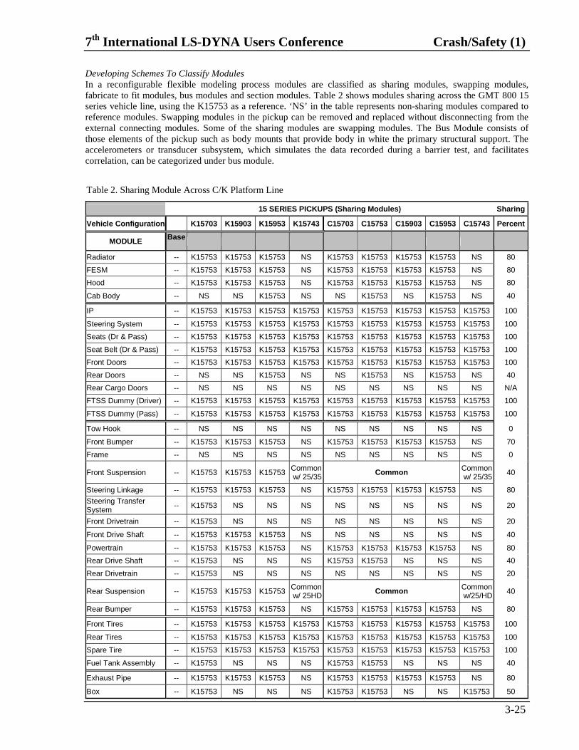
Developing Schemes To Classify Modules In a reconfigurable flexible modeling process modules are classified as sharing modules, swapping modules, fabricate to fit modules, bus modules and section modules. Table 2 shows modules sharing across the GMT 800 15 series vehicle line, using the K15753 as a reference. ‘NS’ in the table represents non-sharing modules compared to reference modules. Swapping modules in the pickup can be removed and replaced without disconnecting from the external connecting modules. Some of the sharing modules are swapping modules. The Bus Module consists of those elements of the pickup such as body mounts that provide body in white the primary structural support. The accelerometers or transducer subsystem, which simulates the data recorded during a barrier test, and facilitates correlation, can be categorized under bus module.

Table 2. Sharing Module Across C/K Platform Line

15 SERIES PICKUPS (Sharing Modules) Sharing

Vehicle Configuration K15703 K15903 K15953 K15743 C15703 C15753 C15903 C15953 C15743 Percent

MODULE Base

Radiator -- K15753 K15753 K15753 NS K15753 K15753 K15753 K15753 NS 80

FESM -- K15753 K15753 K15753 NS K15753 K15753 K15753 K15753 NS 80

Hood -- K15753 K15753 K15753 NS K15753 K15753 K15753 K15753 NS 80

Cab Body -- NS NS K15753 NS NS K15753 NS K15753 NS 40

IP -- K15753 K15753 K15753 K15753 K15753 K15753 K15753 K15753 K15753 100

Steering System -- K15753 K15753 K15753 K15753 K15753 K15753 K15753 K15753 K15753 100

Seats (Dr & Pass) -- K15753 K15753 K15753 K15753 K15753 K15753 K15753 K15753 K15753 100

Seat Belt (Dr & Pass) -- K15753 K15753 K15753 K15753 K15753 K15753 K15753 K15753 K15753 100

Front Doors -- K15753 K15753 K15753 K15753 K15753 K15753 K15753 K15753 K15753 100

Rear Doors -- NS NS K15753 NS NS K15753 NS K15753 NS 40

Rear Cargo Doors -- NS NS NS NS NS NS NS NS NS N/A

FTSS Dummy (Driver) -- K15753 K15753 K15753 K15753 K15753 K15753 K15753 K15753 K15753 100

FTSS Dummy (Pass) -- K15753 K15753 K15753 K15753 K15753 K15753 K15753 K15753 K15753 100

Tow Hook -- NS NS NS NS NS NS NS NS NS 0

Front Bumper -- K15753 K15753 K15753 NS K15753 K15753 K15753 K15753 NS 70

Frame -- NS NS NS NS NS NS NS NS NS 0

Front Suspension -- K15753 K15753 K15753 Common w/ 25/35

Common Common w/ 25/35

40

Steering Linkage -- K15753 K15753 K15753 NS K15753 K15753 K15753 K15753 NS 80

Steering Transfer System

-- K15753 NS NS NS NS NS NS NS NS 20

Front Drivetrain -- K15753 NS NS NS NS NS NS NS NS 20

Front Drive Shaft -- K15753 K15753 K15753 NS NS NS NS NS NS 40

Powertrain -- K15753 K15753 K15753 NS K15753 K15753 K15753 K15753 NS 80

Rear Drive Shaft -- K15753 NS NS NS K15753 K15753 NS NS NS 40

Rear Drivetrain -- K15753 NS NS NS NS NS NS NS NS 20

Rear Suspension -- K15753 K15753 K15753 Common w/ 25HD

Common Common w/25/HD

40

Rear Bumper -- K15753 K15753 K15753 NS K15753 K15753 K15753 K15753 NS 80

Front Tires -- K15753 K15753 K15753 K15753 K15753 K15753 K15753 K15753 K15753 100

Rear Tires -- K15753 K15753 K15753 K15753 K15753 K15753 K15753 K15753 K15753 100

Spare Tire -- K15753 K15753 K15753 K15753 K15753 K15753 K15753 K15753 K15753 100

Fuel Tank Assembly -- K15753 NS NS NS K15753 K15753 NS NS NS 40

Exhaust Pipe -- K15753 K15753 K15753 NS K15753 K15753 K15753 K15753 NS 80

Box -- K15753 NS NS NS K15753 K15753 NS NS K15753 50


3-26

NS - Non-sharing modules

Develop Numbering Schemes For Parts, Materials, And Sectional Properties A finite element module consists of several parts; each part was assigned a material number and a section property number. For example, in the radiator module the parts, associated material and section property numbers, elements, and nodes start at 10,000 and this module can have a maximum of 30,000 elements and nodes. The numbering scheme for various modules shown in Table 3 has been applied to the K15753 model in semi-automated process for demonstration purpose. When a fully automated process has been developed, the numbering scheme may no longer be needed. Currently C/K group has revised this numbering scheme to make it more robust and could be useful across all platforms.

Table 3. Numbering Scheme (semi-automated process) and Modular Modeling Guidelines

REQUIREMENTS GUIDELINES

MODULE NUMBERING SCHEME

MAXIMUM RANGE

OPTIMUM MODULE

SIZE

OPTIMUM ELEMENT

SIZE

QUAD Element Percentage

TRI Element Percentage

Radiator 10,000-40,000 30,000 16,500 15-20 97% 3% FESM 50,000-75,000 25,000 13,000 25-30 92% 8% Hood 100,000-115,000 15,000 8,000 30-35 92% 8% Cab Body 150,000-250,000 100,000 40,000 30-35 85% 15% IP 250,000-280,000 30,000 15,000 25-30 89% 11%

Steering System 290,000-295,000 5,000 3,000 15-20 97% 3% Seats (Dr & Pass) 300,000-320,000 20,000 10,000 20-25 95% 5% Seat Belt (Dr & Pass) 390,000-392,000 2,000 1,000 20 --- --- Front Doors (Dr & Pass) 400,000-440,000 40,000 20,000 30-35 93% 7% Rear Doors (Left & Right) 450,000-460,000 10,000 5,000 30-35 90% 10% Rear Cargo Doors 550,000-560,000 10,000 5,000 30-35 90% 10% FTSS Dummy (Driver) 600,000-650,000 50,000 25,000 N/A --- --- FTSS Dummy (Pass) 650,000-700,000 50,000 25,000 N/A --- --- Tow Hook 700,000-702,000 2,000 1,000 7-10 98% 2% Front Bumper 710,000-713,000 3,000 2,000 30-35 91% 9% Frame 750,000-850,000 100,000 60,000 8-20 94% 6% Front Suspension 850,000-890,000 40,000 10,000 15-20 83% 17% Steering Linkage 900,000-904,000 4,000 1,000 20-30 90% 10%

Steering Transfer System 920,000-921,500 1,500 1,200 20-25 90% 10%

Front Drivetrain 930,000-940,000 10,000 1,500 25-35 85% 15%

Front Drive Shaft 990,000-991,000 1,000 200 40-45 100% ---

Powertrain 1000,000-1008,000 8,000 4,000 40-50 85% 15% Rear Drive Shaft 1020,000-1021,000 1,000 500 40-45 100% --- Rear Drivetrain 1030,000-1035,000 5,000 1,500 25-35 85% 15% Rear Suspension 1050,000-1052,000 2,000 500 30-40 100% --- Rear Bumper 1100,000-1108,000 8,000 4,000 25-35 90% 10% Front Tires 1120,000-1125,000 5,000 2,400 40-45 93% 7% Rear Tires 1130,000-1135,000 5,000 2,400 40-45 93% 7% Spare Tire 1140,000-1142,500 2,500 1,200 40-45 93% 7% Fuel Tank Assembly 1150,000-1160,000 10,000 2,000 20-25 95% 5% Exhaust Pipe 1200,000-1210,000 10,000 2,000 30-40 98% 2% Box 1210,000-1250,000 40,000 30,000 30-40 90% 10%

This table may serve as a modular modeling guideline for other CAE best practices based on modeling practices applied to K15753. Based on diverse C/K pickup and utility product line, each module is limited to the elements in the maximum range. For now, a rigid numbering scheme and maximum ranges are the requirements for a modular process. Based on “single vehicle model concept for multiple test configuration” analysis results [2], a guideline has been set up to keep the module and element sizes optimized and limit to 400,000 elements. The complete full vehicle model required to simulate both structural and occupant simulation. Beside finite element model quality based on aspect ratio, warpage, element internal angles, etc., the modular methodology provides a reasonable percentage of quadrilateral and triangle shell elements a module can have.


3-27

Develop Methodology To Connect Parts And Modules The key is to define the connectivity in a way to install the discipline that allows all of the modules to be connected. There are few basic connecting modules that are shown in Figure 4 are needed to connect internal parts with in a module and during module assembly process. There are five joints provided in LS-DYNA manual [3]. These are spherical joint (SJ), revolute joint (RJ), cylindrical joint (CJ), translation joint (TJ) and universal joint (UJ). To create a joint between parts A and B, both the parts need to be rigid and connecting nodes need to be coincident. In modular process, a joint need to portable and robust. Authors have developed modular joints, which is now portable and users doesn’t have to create joints. Beside joint modules, portable bolt module, shock module, mount module, and cable module were been developed. Spot weld module has been developed but may not be robust in semi-or fully automated process and needs further study. All the connecting modules are positioned at (0,0,0) coordinate. Descriptions of these joint definitions are given below. Conventional Joint Modules Spherical joint - In spherical joint, nodes 1 and 2 are added to extra node set A; and nodes 3 and 4 are added to extra node set B. The extra nodes are made rigid by using material type 20. These two extra node sets forms rigid body A and rigid body B. A joint between rigid body A and rigid body B is formed by nodes 2 and 3. MAT68 beams connect nodes 1 and 2; and nodes 3 and 4. Revolute joint - In revolute joint, massless nodes 5 and 6 are created at the same coordinate as nodes 2 and 3. Nodes 1, 2, and 6 are added to extra node set A and nodes 3, 4, and 5 are added to extra node set B. The extra nodes are made rigid by using material type 20. These two extra node sets forms rigid body A and rigid body B. A joint is formed by nodal pair (2, 5) and (3, 6), where rigid body A and B will rotate relatively to each other along local x-axis. A cylindrical joint, can be formed from spherical joint by nodal pair (2, 5) and (3, 6), where rigid body A and B will translate relatively to each other along x-axis. MAT68 beams connect nodes 1, 2 and 6; and nodes 3, 4 and 5. Universal joint - In universal joint, line drawn between nodes (1, 2) and (3, 4) are perpendicular. At the intersection of two perpendicular lines, massless nodes 5 and 6 are created. Nodes 1, 2 and 5 are added to extra node set A and nodes 3, 4 and 6 are added to extra node set B. The extra nodes are made rigid by using material type 20. These two extra node sets forms rigid body A and rigid body B. A joint is formed between nodal pair (1, 3) and (5, 6) or (2, 3) and (5, 6) or (1, 4) and (5, 6) or (2, 4) and (5, 6). MAT68 beams connect nodes 1, 2 and 5; and nodes 3, 4 and 6. Translation joint - In translation joint, massless nodes 5, 6 and 7 are created at the same coordinate as nodes 2, 3 and 4. The line drawn between nodes 3 and 4 or 6 and 7 must be perpendicular to nodes 2 and 3 or 5 and 6. Nodes 1, 2, 6 and 8 are added to extra node set A and nodes 3, 4, 5 and 7 are added to extra node set B. The extra nodes are made rigid by using material type 20. These two extra node sets forms rigid body A and rigid body B. A joint is formed by nodal pair (2, 5), (3, 6) and (7, 8) where rigid body A and B will translate relatively to each other along local x-axis. MAT68 beams connect nodes 1, 2, 6 and 8; and nodes 3, 4, 5 and 7. Body Mount Module The interaction between the frame and the major components and assemblies attached to it has a significant effect on overall vehicle behavior. It is important that the mounts, which control such interaction, are represented well. In frontal impact the primary concern is relative motion in the fore-aft axial direction and accordingly it is possible to use a single spring element to represent the force-deflection characteristic for each mount along this axis. However, in modular approach a full vehicle model is essentially a single model to be used for all test modes. Therefore, there will be need for three spring properties along all three axes. A single beam material type 68, which has all six degree of freedom, can be used instead of three springs. The accuracy of spring or beam element representation relies solely on the loading and unloading characteristic of a physical mount. The approach that has been adopted to obtain characteristic of beam representing any mounts involves the use of accelerometers data from full vehicle crash tests. Spare Tire Connecting Module The spare tire is generally connected to the rear frame by a cable. Sometimes in the test spare tire cable tears and comes off. This physical situation can be modeled by combining cable discrete beam type 71 and plastic-elastic discrete beam type 68.

Typ

es o

f M

od

ula

rize

d J

oin

ts

M

28

S

hock

abs

orbe

r m

odul

e

Co

mb

inat

ion

of

Mo

du

lari

zed

Jo

ints

A

B

J

1

2

3

4

5

6

x y

z x

y z

Rev

olut

e jo

int/

Cyl

indr

ical

Joi

nt

A

B

J

2

3

4

x y

z

1

Sphe

rica

l Joi

nt

A

B

J

2

5

7

4

8

6

1 x

y z

x y

z 3

Tra

nsla

tion

Joi

nt/ L

ocki

ng J

oint

4

1

2

3

x y

z

A

6

5

B

x y

z

U

nive

rsal

Jo

int

A

B

J 2

3

4

x y

z

1

Sphe

rica

l Joi

nt

4

1

2

3

x y

z

A

6

5

B

x y

z

Uni

vers

al

Join

t

A

B

J

2

5

7

4

8

6

1

x y

z

x y

z

3

Tra

nsla

tion

Joi

nt/ L

ocki

ng J

oint

A

B

J 2

3

4

x y

z

1

Sphe

rica

l Joi

nt

A

B

J 1

2

3

4

5

6

x y

z

x y

z

Rev

olut

e jo

int/

Cyl

indr

ical

Joi

nt

A

B

J 2

3

4

x y

z

1

Sphe

rica

l Joi

nt

A

B

J 2

3

4

x y

z

1

Sphe

rica

l Joi

nt

A

B

J 2

3

4

x y

z

1

Sphe

rica

l Joi

nt

Rev

olut

e jo

int/

Cyl

indr

ical

Joi

nt

Rev

olut

e jo

int/

Cyl

indr

ical

Joi

nt

A

B

J 1

2

3

4

5

6

x y

z

x y

z

A

B

J 1

2

3

4

5

6

x y

z

x y

z

Rev

olut

e jo

int/

Cyl

indr

ical

Joi

nt

A

B

J

2

5

7

4

8

6

1

x y

z

x y

z

3

Tra

nsla

tion

Joi

nt/ L

ocki

ng J

oint

A

B

J 1

2

3

4

5

6

x y

z

x y

z

Rev

olut

e jo

int/

Cyl

indr

ical

Joi

nt

4

1

2

3

x y

z

A

6

5

B

x y

z

Uni

vers

al

Join

t

A

B

J 1

2

3

4

5

6

x y

z

x y

z

4

1

2

3

x y

z

A

6

5

B

x

y z

Uni

vers

al

Join

t

4

1

2

3

x y

z

A

6

5

B

x

y z

Uni

vers

al

Join

t

A

B

J

2

5

7

4

8

6

1

x y

z

x y

z

3

Tra

nsla

tion

Joi

nt/ L

ocki

ng J

oint

A

B

J

2

5

7

4

8

6

1

x y

z

x y

z

3

Tra

nsla

tion

Joi

nt/ L

ocki

ng J

oint

4

1

2

3

x y

z

A

6

5

B

x

y z

Uni

vers

al

Join

t

A

B

J

2

5

7

4

8

6

1

x y

z

x y

z

3

Tra

nsla

tion

Joi

nt/ L

ocki

ng J

oint

Spar

e T

ire

Con

nect

ing

Mod

ule

B

ody

Mou

nt M

odul

e

M71

M68

x

y

z

x

y

z

x

y

z

x

y

z

M

68

Sp

ot w

eld

mod

ule.

Gap

< 5

mm

.

Bo

lt

Mo

du

les

Sp

ot

Wel

d

Mo

du

les

Cab

le J

oin

t M

od

ule

M

ou

nt

Mo

du

le

x

y

z

Sh

ock

M

od

ule

s

x

y

z

M

28

x

y

z

M

68

B

olt

mod

ule

used

in c

onne

ct-

in

g fo

rged

and

die

cas

t pa

rts;

thic

k sh

eet

met

als.

Bea

m

le

ngth

> 5

mm

.

B

olt

mod

ule

used

in c

onne

ct-

in

g sh

eet

met

als;

she

et m

etal

to

forg

ed o

r ca

st p

art.

Bea

m

L

engt

h <

5 m

m.

Figu

re 4

. Bas

ic C

onne

ctin

g M

odul

es


3-29

Material type 71 permits elastic cable to be realistically modeled with no force developing in compression, i.e. force generated by the cable is nonzero if and only if the cable is in tension. For a slack cable the offset is input as a negative length. The area and offset are defined on either the cross-section or element cards. For beam material type 71, a load curve defined as engineering stress versus engineering strain is specified. Failure criteria in material type 71 elastic beam cannot be specified and so a 1 mm long plastic-elastic beam type 68 is connected between the rigid body of the tire hub and one end of the elastic beam. Failure criteria are specified based on a force/ moment criterion and a displacement/ rotational criterion. Bolt Module A bolted connection between solid-to-solid blocks is represented by Belytschko-Schwer resultant beam element with minimum two integration points. A resultant plasticity material type 28 has been used. Beam length needs to be greater than 10 mm. The cross sectional properties of beam elements vary depending on the diameter of the bolt. A bolted connection between sheet-to-sheet metal or sheet metal -to-solid block is represented by plastic-elastic beam type 68. Here beam element can be failed with out tearing sheet metal and beam length can be less than 1mm. This beam doesn’t enter in to time step calculation. Illustration Of Connectivity Any connecting module is described in a separate portable key word file with coordinate information of the connecting points, coordinate information of the reference node, material and sectional properties of the beam. Figure 5 illustrates how a bumper bracket is connected to the frame by four bolt connecting module. Nodes (1,4) and (5,8) are the connecting points in the frame; and nodes (2,3) and (6,7) are the connecting points in the bumper brackets. These node definitions are commented out in the LSDYNA connecting module deck when integrated with all other modules because these nodes are integral part of the frame and brackets. Nodes (9,10,11,12) are the reference nodes of the beam elements. During renumbering and positioning, these nodes are active.

Module Assembly For Job Submission The template to assemble all vehicle and associated connecting modules, barrier module, global contact module, and control card module, is essentially a LSDYNA deck, which is illustrated in Table 4. Directory architecture must be well planned to make modules portable by proper naming and numbering convention. Module Library All the modules described in this report are stored in C/K global directory. There are 8 sub-directories in it – vehicle module directory, connecting module directory, control card directory, velocity directory, barrier directory, contact directory, output directory and instrumentation directory. User can run job remotely by submitting DYNA assembly deck. The results will be dumped from where job has been submitted. In this process user only needs DYNA assembly deck and job submission script. User’s doesn’t need to have all the modules in his or her directory except the modules that are being worked up on.

9

11

10 4

3

2

1

Left bracket to frame

Holes in the frame (1,4)

Holes in the bracket (2,3)

8

7

6

5

Right bracket to frame

Holes in the frame (5,8)

Holes in the bracket (6,7)

12

Figure 5. Illustration of Bolt Module Connection


3-30

Develop Flexible Process Flow In Agile Organization Flexibility can be achieved in a modeling system in which parts can be added, removed and replaced with minimum disruption. Reconfigurability can be achieved by carefully defining the contents of each module by physical parts and all users maintaining a disciplined approach to connectivity. Flexibility and Reconfigurability in a modular methodology can be achieved [1]. If any simulation organization wanted to be agile, then they should be capable of operating profitably in a competitive environment of continually, and unpredictably, changing customer opportunities. In that ideal organization if an individual wanted to be agile then he or she should be capable of contributing to the bottom line of a company that is constantly reorganizing its human and technological resources in response to unpredictably changing customer opportunities. We began with a strategic vision of what we needed to accomplish from a business standpoint. Then we built an ideal infrastructure plan to support that vision. The agile organization integrates employees, contractors, customers, and suppliers to share knowledge and skills. The infrastructure can be built on web based simulation technology. The foundation is based on a standardized, enterprise-wide platform designed to transform the business relationship with various user constituents. The web based simulation technology will enable rapid deployment of various application software which will make the internal users interact with each other and also make GM extremely easy to do analysis business with suppliers.

DISCUSSION OF RESULTS A modular single full vehicle finite element model K15753 was built from design data and the vehicle was simulated to the test configuration under frontal, angle, rear, ODB (EEC), ODB (IIHS), offset rigid barrier (35 mph and 40 mph) and vehicle to vehicle front 40% offset impact condition [2]. Vehicle tested in front, left angle, rear and

ODB (EEC) had different masses and is a beta or prototype version. FE model was not representative of these individual test vehicles and modular modeling effort started long after the vehicles have been tested. An average of test vehicle masses was used as a base line for the FE full vehicle model. In the near future, modules will become more detailed and module mass will dictate the vehicle mass, inertia and center of gravity.

303 313

225 234 222 209

305 286

397

305

397

675

0

100

200

300

400

500

600

700

800

FRONT

C1173

3

REAR

C1227

2

ODB - 40

ORB - 35

ORB - 40

VEH - VEH

EN

ER

GY

(K

J)

TEST ANALYSIS

Figure 6. Initial Impact Energy

FRONT ANGLE REAR ODB (EEC)

ODB (IIHS)

ORB (35)

ORB (40)

VEH TO VEH


3-31

0 20 40 60 80 100 120 140 160 180

Radiator

Fesm

Hood

Cab

Inst. Panel

Steering

Seat (D&P)

Left F. Door

Right F. Door

Right R. Door

Box

Front Chassis

Mid Chassis

Rear Chassis

Tow Hook

Front Bumper

Left F. Susp.

Right F. Susp.

Left F. Shock

Right F. Shock

Stabilizer

Steer Linkage

Steer Gear

Front Drivetrain

Pow ertrain

Exhaust

Front Drive Shaft

Rear Drivetrain

Rear Drive Shaft

Rear Suspension

Left R. Shock

Right R. Shock

Rear Bumper

Fuel Tank Assy.

Front Tires

Rear Tires

Spare Tires

ENERGY (KJ)

IIHS

NCAP

Figure 7. Module Internal Energy Distribution


3-32

A full vehicle finite element model doesn’t always represent a test vehicle because models don’t get updated as quickly as retrofitting a new part in a test vehicle. In an agile organization updating modules might be possible depending up on management’s skills, experience and positive thinking. If test vehicle is representative of analytical model (which means analysis is done before testing and all the physical parts are well represented in the model), test and analytical data may be closer. We also know that two identical test vehicle in any impact situation never produce same data. There also uncertainty is involved. So, when analysis data is compared with test data from two identical test vehicles under same impact mode, analysis results can be conservative. In figure 6, analysis and test vehicle initial impact energy is not exact because FE full vehicle model mass is fixed. The impact energy variation from test in each test configuration is with in ± 20 KJ. Figure 7 provides the energy absorbed by each of the modules given in Table 3 in full frontal and ODB offset impact scenario.

Figure 8. Crash Events at 35 mph (Front Impact)

Figure 9. NCAP Barrier Force-Time and Force-Displacement


3-33

In figure 8 we have shown various crash events at 35 mph, which influences the NCAP results. Figure 9 compares analysis and test NCAP barrier force-time and force-displacement data. Figures 10 and 11 compare left and right rear rocker acceleration between analysis and test in left angle impact at 30 mph; and in ODB impact at 40 mph. Analysis results could not be compared to ODB (IIHS) offset rigid barrier (35 mph and 40 mph) and vehicle-to-vehicle impact test data. Analysis engine intrusion in front and angle impact is very close to the test.

Responsibilities to be taken by the users Users following modular methodology need to understand very clearly the modular concept, process and the current limitations that are outlined in this report. Contact Definition. For any impact condition, there is only one global single contact interface card by parts, which has been defined. The global single contact interface should exclude the occupant and restraint system parts. To model complex restraint system performance and occupant interactions with the vehicle interior, multiple contact modules, surface to surface contact interfaces are defined. For inflatable restraints, contact interface are defined

Figure 10. Left and Right Rear Rocker Acceleration in Angle Impact

Figure 11. Left and Right Rear Rocker Acceleration in Offset Impact (IIHS)


3-34

between air bags and windshield, driver and steering wheel, dummy head, chest and arms with the driver air bag. Passenger air bag is not modeled and needs development. Other occupant contact interfaces are defined between pelvis and seats, knee and knee bolster, feet and floor pan/toe board, and the dummies chest and pelvis with the seta belts. When building a module, users must add single surface contact card by parts that represents shell components. After creating this card dollar it out. Automatic inclusion of all parts by box is not recommended. This might cause instabilities when dummies are brought into the model because pre-defined dummy contacts might see duplicate contact definition. There are two ways to make modular global contact – (i) create a LS-DYNA file for global contact definition and then add parts from the contact card definition there in the individual modules, (ii) read module assembly deck or individual modules in HYPERMESH [4]. Switch off all other elements except shells. Create part set and export this file. Extract part set from the exported file and add to the single contact card definition of the global contact file. In the beginning users will have difficulties but once they understand the concept, the modeling process will appear easy. The mechanical way of modularizing the contact definition is very close to the automated process that is described in the earlier sections. Velocity Definition. Velocity of any moving object is defined by box. All nodes with in the box will have the prescribed velocity. Velocity module card has box dimension and velocity magnitude in mm/millisecond. There can be many velocity module files representing 9mph, 25 mph, 30 mph, 34 mph, etc. If vehicle coordinate doesn’t change then user need not worry. However if vehicle position has been changed then user need to know vehicle size, i.e.: xmin, xmax; ymin, ymax; and zmin, zmax. Replace the box definition by current dimensions. The above descriptions holds good for moving barriers. Local Coordinates Mobility. Local coordinates are used in all the basic connecting modules. It is necessary to translate or rotate these modules in HYPERMESH to connect parts. HYPERMESH cannot translate or rotate the local coordinates with other element definition at the same time. This is because LS-DYNA local coordinate definition by nodes is not an available feature in HYPERMESH. This unavailable feature can make the user frustrated. There is way to get away with this limitation but users need to be careful. User needs to know the beam element (mat 68) that is connecting two points in HYPERMESH. Use three nodes that are used to define the beam in local coordinate definition by nodes. Design Iteration. In the design iteration user can only sub-modularize a part or group of parts that are bolted to other parts. If the connecting points remain same than only mesh will change. Some time new part may be added or deleted from the existing module. This will cause the module to be renumbered. If users follow proper numbering scheme, contact module definition, and connecting methodology described in this report; following the modular concept will be easier. Use of EASi-CRASH. EASi-CRASH [5] is one of the available tool today that can read and renumber all the LS-DYNA crash related cards completely except *INTEGRATION BEAM. Use EASi-CRASH for module renumbering and deleting unwanted referred cards.

SUMMARY The Modular approach and the strategies developed in GM is a unique methodology for building full vehicle finite element models, which allows the use of a single vehicle model, assembled using component modules, to simulate multiple test configurations. The benefits of new reconfigurable and flexible process described in the modular process are –

• Quicker model assembly and setup times: Models can be built at least partially from modules representing carryover components. Incorporating new or modified hardware can be accomplished by updating the affected modules and reassembling them into the full vehicle model.

• Reduced storage requirements: Storing the individual building blocks for a complex program one time each on a common server for use by any analyst working on the project will require less space than storing complete vehicle models of each important configuration.

• Reduced training time for new engineers to become productive: New engineers can be assigned to update or create simpler modules, and thus contribute productively, before they have the experience or ability to effectively model complex modules such as the frame.


3-35

• Sharing of common component models among vehicle platforms: A module representing an engine, seat, or other component that is shared among model lines can be updated once and the updated version used immediately by all the platforms the changes affect.

• Facilitates updates to specific hardware: Changing the design of a bumper or door means that only the affected module needs to be updated. All vehicle configurations can then use the updated module. In the current system many individual FVM’s would need to be updated.

• Promotes increased reliance on math-based strategy: Use of modularity leads to earlier availability of full vehicle finite element analysis early in a program as new vehicle structure is being defined because modules representing the new structure can be evaluated in the old model before the entire new structure is available, and faster response to updates during the design phases where change is most likely to occur.

No alternative exists to accomplish the same results as this modular process. Adaptation of this modular process can aid finite element simulation group to be more efficient, cost effective and to be in competitive advantage.

ACKNOWLEDGEMENT The authors would like to specially acknowledge Dilip Bhalsod of LSTC for committing the time and effort to go through the modular concepts, process and connecting modules. He has helped to address users issues and concerns; and the limitations of the mechanical modular process that user should know. Authors wanted to acknowledge Andrew R. Dwoinen, Scott Mc Donald, Dan Motowski and Rajesh Parmer for their support to modular modeling concept and coming up with a robust modular numbering scheme. Authors like to convey a special thanks to Andrew R. Dwoinen for his constructive criticisms while going through the report. Finally, this work wouldn’t have completed with out the support received from Mark O. Ellis.

REFERENCES

1. Dhar, S. D., Hohnstadt, W. E., and Green, J. D., (2002). “Integrated Modular Methodology – Philosophy & Strategy to Build Full Vehicle Finite Element Model,” GM Technical Report, pp. 1-67.

2. Dhar, S. D., and Hohnstadt, W. E., (2000). “Application of Single Finite Element Vehicle Model For Multiple Test Configuration – A Modular Approach,” CSTEM Presentation (GM Internal Conference).

3. LS-DYNA user’s manual, November 14, 2001, Version 960. 4. Altair HyperMesh Version 4.02, 2000, Altair Engineering. 5. EASi-CRASH Version 1.5 LSDYNA, 16th October 2000, Easi Engineering.


3-36

Modular Strategy To Build Full Vehicle Finite Element Model

Documents

Transcript of Modular Strategy To Build Full Vehicle Finite Element Model