Modélisation de la dégradation chimique de membranes dans ...
229
HAL Id: tel-00767412 https://tel.archives-ouvertes.fr/tel-00767412 Submitted on 19 Dec 2012 HAL is a multi-disciplinary open access archive for the deposit and dissemination of sci- entific research documents, whether they are pub- lished or not. The documents may come from teaching and research institutions in France or abroad, or from public or private research centers. L’archive ouverte pluridisciplinaire HAL, est destinée au dépôt et à la diffusion de documents scientifiques de niveau recherche, publiés ou non, émanant des établissements d’enseignement et de recherche français ou étrangers, des laboratoires publics ou privés. Modélisation de la dégradation chimique de membranes dans les piles à combustibles à membrane électrolyte polymère Romain Coulon To cite this version: Romain Coulon. Modélisation de la dégradation chimique de membranes dans les piles à combustibles à membrane électrolyte polymère. Autre [cond-mat.other]. Université de Grenoble, 2012. Français. NNT : 2012GRENY023. tel-00767412
Transcript of Modélisation de la dégradation chimique de membranes dans ...

HAL Id: tel-00767412https://tel.archives-ouvertes.fr/tel-00767412
Submitted on 19 Dec 2012
HAL is a multi-disciplinary open accessarchive for the deposit and dissemination of sci-entific research documents, whether they are pub-lished or not. The documents may come fromteaching and research institutions in France orabroad, or from public or private research centers.
L’archive ouverte pluridisciplinaire HAL, estdestinée au dépôt et à la diffusion de documentsscientifiques de niveau recherche, publiés ou non,émanant des établissements d’enseignement et derecherche français ou étrangers, des laboratoirespublics ou privés.
Modélisation de la dégradation chimique de membranesdans les piles à combustibles à membrane électrolyte
polymèreRomain Coulon
To cite this version:Romain Coulon. Modélisation de la dégradation chimique de membranes dans les piles à combustiblesà membrane électrolyte polymère. Autre [cond-mat.other]. Université de Grenoble, 2012. Français.NNT : 2012GRENY023. tel-00767412

THÈSE
Pour obtenir le grade de
DOCTEUR DE L’UNIVERSITÉ DE GRENOBLE
Spécialité : Physique
Arrêté ministériel : 7 août 2006
Présentée par
Romain COULON Thèse dirigée par Alejandro A. Franco et préparée au sein du Laboratoire des Composants pour les piles à combustibles, les électrolyseurs et de modélisation. (Commissariat à l’Energie Atomique et aux Energies Alternatives) et de l’Institut de thermodynamique technique (Deutsches Zen-trum für Luft und Raumfahrt) dans l'École Doctorale de Physique
Modélisation de la dégradation chimique de membranes dans les piles à combustible à mem-brane électrolyte polymère.
Thèse soutenue publiquement le 31 janvier 2012, devant le jury composé de :
Michael EIKERLING Professeur, Simon Fraser University, Vancouver, Rapporteur
Gérald POURCELLY Professeur d’Universités, Université de Montpellier 2, Rapporteur
Thierry DEUTSCH Docteur chercheur, Université Joseph Fourier, Grenoble, Président
Jochen KERRES Docteur chercheur, Universität Stuttgart, Examinateur
Gwenaelle RENOUARD-VALLET Ingénieur, Airbus, Hambourg, Examinateur
Wolfgang G. BESSLER Co-encadrant de thèse, ingénieur chercheur, DLR Stuttgart
Alejandro A. FRANCO Directeur de thèse, ingénieur chercheur senior, CEA Grenoble

Abstracts
i
Abstracts
Resumé en français :
Cette thèse propose une approche de modélisation de la dégradation chimique par attaque radicalaire
de la membrane dans les piles à combustibles à membrane électrolyte polymère, ainsi que à son impact
sur la dégradation de la performance électrochimique.
La membrane considérée dans cette étude est de type perfluorosulfonique, avec une structure dépen-
dant fortement de son humidification et conditionnant les propriétés de transport. Afin d’étudier la
dégradation de la membrane, il faut dans un premier temps établir un modèle de transport, qui sera
utilisé aussi bien dans le modèle de dégradation que par les modèles de performance de cellule déjà
existants. Une fois ce modèle établi, nous nous focalisons sur la partie dégradation chimique. Après
une compréhension globale des phénomènes physico-chimiques se déroulant lors de la dégradation,
une mise en équation détaillée est nécessaire. Même les concepts utilisés sont relativement simples, le
besoin de nombreux paramètres nous a contraint à simplifier le modèle sur certains points, notamment
le mécanisme de dégradation chimique, tant la complexité du phénomène est un frein à la paramétrisa-
tion du modèle. Ce modèle, avec ses simplifications et ses hypothèses, est ensuite validé, aussi bien
d’un point de vue performance que d’un point de vue dégradation.
Il est pour finir exploité dans différents cas de figures, allant de l’utilisation ininterrompue à courant
constant (test purement utilisé en laboratoire) à un cyclage plus représentatif de conditions de fonc-
tionnement réelles.
PEMFC, Pile à combustible, Fenton, Dégradation, Modélisation, Membrane, Nafion®
Abstract in English:
This thesis proposes a modeling approach of the chemical degradation by radicals attack of the mem-
brane in polymer electrolyte membrane fuel cells, as well as its impact on the electrochemical perfor-
mance degradation. The work considers a perfluorosulfonated acid type membrane. Its structure is
strongly influenced by humidification, which also impacts the transport properties of mass and charge
within the membrane. In order to study the degradation of the membrane, we first established a multi-
species transport model for protons, water, and dissolved gases, radicals and ions. We then included
detailed chemical reaction mechanisms of hydrogen peroxide formation, hydrogen peroxide decompo-
sition, and radical attack of the membrane. Finally, a feedback between degradation, structure, and
performance was established. Parameters were identified and the model was validated using literature
experimental data both under performance and degradation aspects.
The model was then exploited under different conditions, from pure laboratory conditions (constant
current kept over a long time) to working conditions which are more representative of the use of a
PEMFC for stationary applications (performance cycles).
Polymer electrolyte membrane fuel cell (PEMFC), Fenton, Degradation, Modeling, Nafion®


Remerciements / Danksagung
iii
Remerciements / Danksagung
Trois ans c’est le temps nécessaire à terminer le lycée. C’est aussi le temps nécessaire à terminer une
école d’ingénieur. Mais ce fut également le temps nécessaire à l’aboutissement de ce projet de thèse.
En premier lieu, je tiens ici à remercier les membres du jury. Mes rapporteurs, Michael Eikerling et
Gerald Pourcelly, pour le temps qu’ils m’ont accordé, à la fois lors de la révision de mon manuscrit et
également lors de leur présence à ma soutenance. Ich bedanke mich auch bei Jochen Kerres, für seine
Anwesenheit bei der Verteidigung und sein große Interesse an meiner Arbeit. Je voudrais également
remercier Gwenaelle Renouard-Vallet et Nicolas Fouquet pour le temps qu’ils m’ont accordé à lors de
l’examen de mon manuscrit. Et merci à Thierry Deutsch, qui fut un temps mon directeur de thèse.
Ensuite viennent ceux qui me soutiennent et supportent depuis 3 ans (voire plus). Alejandro et Wolf-
gang, merci pour votre soutien au cours de cette aventure, et merci surtout pour la chance que vous
m’avez donnée il y a trois ans, alors que je n’avais jamais programmé, ni su ce qu’était une pile à
combustible. Vos contributions et toutes les discussions enrichissantes que nous avons pu avoir ont
grandement contribué à combler mes lacunes.
Nun meine Gedanken an meiner deutschen Kumpel ! Danke Dir Christian fürs vieles Lachen, Brainst-
orming und Freitags-LKW! Danke auch der Modellierungsgruppe und alle, die mal dabei waren: Jo-
nathan, David, der kleine Wolfgang, Vitaliy Cheng, Max, Florian, Moritz, Wendelin, Christoph und
noch viel mehr, da es viele waren.
Ensuite les „français“, parce que pas beaucoup ne sont français. Obrigado les brésiliens Luiz, Daiane
et Rodriginho pour m’avoir fait découvrir les paçoquinha et pour votre bonne humeur au labo. Alegato
Yoshinori, your help was first quality in solving physical issues the last months. Grazie Valentina, je
note que je dois arrêter les T shirt moches et me mettre aux chemises. Thank you professeur Cheah.
Greetings Senthilnathan. Gracias Pablo, don’t forget that fairy wear boots in a locomotive breath.
Merci également à Fus Ro Dah Benjamin, pour les quizz, les séquences vintage et sa contribution dans
ma quête de faire découvrir la culture française à nos brésiliens. Merci ensuite aux « autres », ceux qui
font des expériences… Nicolas, Olivier, Zhe, Federico, Anne-Gaëlle, Galdric, Samir, Mohamed, etc
etc. Merci à mes secrétaires successives, qui ont dû endurer ma présence plus qu’envahissante dans
leur bureau. Donc merci à vous, Gégé, Kim, Aline et Charline ! Un merci tout particulier également à
Mathias, tu as beau faire des modèles, tu n’en restes pas moins un bon vosgien et merci à Jenny pour
les heures passées à discuter et à rigoler.
Pour terminer, les derniers remerciements mais non les moindres, je remercie mon papa, ma maman,
mon brud et ma ninette pour leur soutien moral non scientifique depuis toutes ces années passées et à
venir. Je leur dédie ce manuscrit qu’ils ne comprendront jamais.


v
« La théorie, c'est quand on sait tout et que rien
ne fonctionne. La pratique, c'est quand tout
fonctionne et que personne ne sait pourquoi.
Ici, nous avons réuni théorie et pratique : Rien
ne fonctionne... et personne ne sait pourquoi! »
Albert Einstein
«C’est pas faux»
Perceval, Kaamelot


Table of Contents
vii
Table of Contents
Abstracts ................................................................................................................................................... i
Table of Contents .................................................................................................................................. vii
List of Tables .......................................................................................................................................... xi
List of Figures ....................................................................................................................................... xii
List of Abbreviations ............................................................................................................................ xix
List of Symbols .................................................................................................................................. xxiii
0 Introduction ..................................................................................................................................... 3
0.1 What is modeling? Why using modeling in fuel cell technology? .......................................... 3
0.2 Scope of this thesis .................................................................................................................. 4
1 Context and motivation of this thesis: Membrane Degradation in PEMFC .................................... 8
1.1 A clean energy conversion device: The PEMFC..................................................................... 8
1.1.1 General presentation ........................................................................................................ 8
1.1.2 Components of a PEMFC ................................................................................................ 9
1.2 Nafion®: The first and most famous electrolyte for PEMFC ................................................ 12
1.2.1 An enigma for modelers and polymer scientists ........................................................... 12
1.2.2 Analytical methods for morphology determination of Nafion® .................................... 14
1.3 Chemical degradation of the electrolyte in PEMFCs: Experimental evidence ..................... 22
1.3.1 Loss of cell performance over time ............................................................................... 22
1.3.2 Membrane thinning ....................................................................................................... 26
1.3.3 Production of hydrogen peroxide in the electrodes ....................................................... 30
1.3.4 Formation of radicals ..................................................................................................... 33
1.3.5 Chemical analysis of the degradation of PFSA membranes .......................................... 34
1.4 Chemical degradation of the electrolyte in PEMFCs: Available modeling work ................. 35
1.5 Summary ............................................................................................................................... 41
2 Modeling of the chemical degradation of the PFSA membrane.................................................... 47
Table of Contents
viii
2.1 Introduction ........................................................................................................................... 47
2.2 Modeling the transport processes in the membrane .............................................................. 47
2.2.1 Modeling of water management and transport .............................................................. 47
2.3 Modeling of chemical degradation of Nafion® ...................................................................... 58
2.3.1 Chemical mechanism for Nafion® degradation ............................................................. 58
2.3.2 Mathematical formulation of the chemical degradation ................................................ 61
2.3.3 Proton transport in the membrane ................................................................................. 65
2.4 Summary ............................................................................................................................... 69
3 Coupling of the membrane model with electrode and cell models ............................................... 73
3.1 Why cell models? .................................................................................................................. 73
3.1.1 DENIS ........................................................................................................................... 73
3.1.2 MEMEPhys® ................................................................................................................. 73
3.1.3 Membrane simulation code ........................................................................................... 74
3.2 Physics underlying the MEMEPhys® model ......................................................................... 75
3.2.1 Presentation of the model .............................................................................................. 75
3.2.2 Description of the multi scale model of the electrodes.................................................. 76
3.2.3 Calculation of the potential in the MEMEPhys® approach ........................................... 80
3.2.4 Coupling of the MEMEPhys® electrode model with electrochemistry ......................... 83
3.2.5 Channel and GDL model ............................................................................................... 87
3.3 Physics underlying in the electrode model of DENIS ........................................................... 88
3.3.1 Presentation of the model .............................................................................................. 88
3.3.2 Calculation of the cell potential in DENIS .................................................................... 89
3.3.3 Gas transport and channel model in DENIS .................................................................. 93
3.4 Comparison MEMEPhys® / DENIS electrode models .......................................................... 94
3.5 Coupling of the membrane model with the electrodes model ............................................... 96
3.5.1 Generalities .................................................................................................................... 96
3.5.2 Specifications for the coupling in DENIS ..................................................................... 96
Table of Contents
ix
3.5.3 Specifications for the coupling in MEMEPhys® ........................................................... 97
3.6 Summary ............................................................................................................................... 99
4 Results and discussion ................................................................................................................. 103
4.1 Introduction ......................................................................................................................... 103
4.2 Model parameterization and validation ............................................................................... 105
4.2.1 Presentation of the “standard” cell used in the simulations ......................................... 105
4.2.2 Electrochemical model ................................................................................................ 107
4.2.3 Chemical degradation model ....................................................................................... 110
4.2.4 Influence of experimental conditions on chemical degradation .................................. 120
4.2.5 Validity of the model ................................................................................................... 122
4.3 Impact of chemical degradation on cell performance under constant current load ............. 123
4.3.1 Introduction ................................................................................................................. 123
4.3.2 Impact of the chemical degradation on cell potential and membrane resistance ......... 123
4.3.3 Impact of the chemical degradation on cell performance: Evolution of the polarization
curve 139
4.3.4 Localization of the degradation in the membrane ....................................................... 146
4.4 Impact of chemical degradation on cell performance under cyclic current operation ......... 147
4.4.1 Introduction to the necessity of the use of current cycles ............................................ 147
4.4.2 On-off cycle of a PEMFC ............................................................................................ 148
4.4.3 Imin–Imax cycle of a PEMFC ......................................................................................... 152
4.5 Impact of the presence and the amount of iron ions on degradation ................................... 156
4.6 Degradation of other PFSA membranes .............................................................................. 160
4.7 Prediction of long-term cell durability ................................................................................ 164
4.8 Strategies for mitigating membrane degradation ................................................................. 168
4.8.1 Sensitivity analysis ...................................................................................................... 168
4.8.2 Experimental conditions preventing the PFSA membrane chemical degradation ...... 170
4.8.3 Operating conditions for a higher durability of the PFSA membrane ......................... 171
4.8.4 Type of membranes which are the less sensitive to chemical degradation ................. 171

Table of Contents
x
4.9 Outlook: Simulations of the membrane model in DENIS environment .............................. 172
5 Summary and conclusions ........................................................................................................... 173
Appendix A: On Nafion®®
and the determination of the chemical structure of a PFSA membrane ... 177
Appendix B: About Fenton chemistry, its application and its complexity .......................................... 179
Appendix C: Sensitivity analysis of the chemical degradation model ................................................ 181
Appendix D: Parameters used during the simulations......................................................................... 183
References ........................................................................................................................................... 187

List of Tables
xi
List of Tables
Table 1.1: Materials and properties of the PEMFC components........................................................... 10
Table 1.2: Parameters of some commercial PFSA membranes (when no value for a parameter is given,
this means that the parameter is not present in the chemical structure of the ionomer) ........................ 14
Table 1.3: Evolution of membrane thickness of Nafion® membranes exposed in H2 or O2 for 1000 h
(after [71]) ............................................................................................................................................. 27
Table 1.4: AST used by Young et al. [16]. ........................................................................................... 29
Table 3.1: Summary of the potentials calculated in the MEMEPhys® model ....................................... 79
Table 3.2: DENIS – MEMEPhys® models: comparison of the general features as used in this PhD
thesis work. ............................................................................................................................................ 95
Table 4.1: Variable parameters in the simulations .............................................................................. 106
Table 4.2: Main structural parameters of our standard PEMFC ......................................................... 106
Table 4.3: Gibbs activation energies for elementary steps (chemical and electrochemical) for the HOR
and the ORR. ....................................................................................................................................... 107
Table 4.4: Parameter used in the experiment displayed in Figure 4.5. ................................................ 109
Table 4.5: Experimental parameters used by Liu and Zuckerbrod ...................................................... 111
Table 4.6: Gibbs activation energies for elementary steps for the H2O2 formation ............................ 112
Table 4.7: Experimental parameters used by Aoki et al...................................................................... 114
Table 4.8: Kinetic rates of Fenton's chemistry used in our model ...................................................... 114
Table 4.9: Experimental parameters used by Young et al. for the determination of cumulative fluoride
ions released under AST. ..................................................................................................................... 117
Table 4.10: Thermal evolution of the side chain degradation kinetic rate .......................................... 119
Table 4.11: Conditions used for the on - off simulations .................................................................... 149
Table 4.12: Conditions used for the Imin–Imax simulations ................................................................... 154
Table 4.13: Parameters of membranes simulated in this study ........................................................... 161
Table 4.14: Extra parameters regarded for the accurate study of the influence of membrane type. ... 163

List of Figures
xii
List of Figures
Figure 1.1: Basic diagram of a PEMFC [40] ........................................................................................... 9
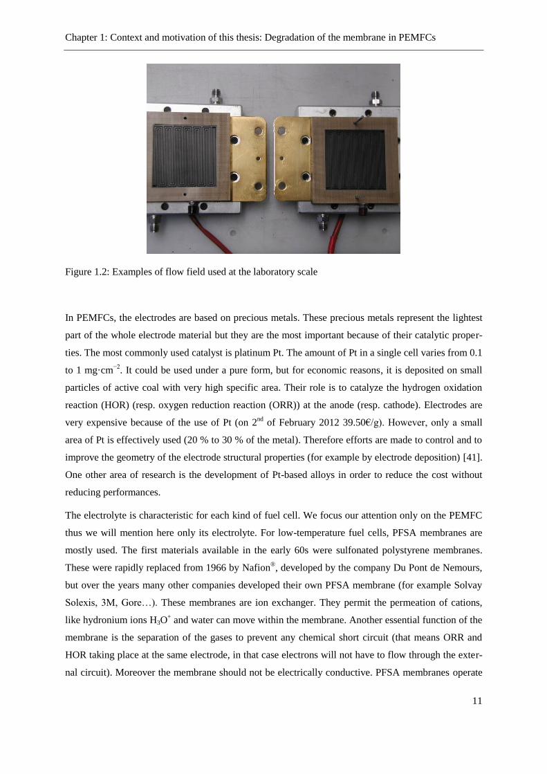
Figure 1.2: Examples of flow field used at the laboratory scale ........................................................... 11
Figure 1.3: General formula of a PFSA membrane ............................................................................... 13
Figure 1.4: Cluster-network model from Gierke [59]. .......................................................................... 16
Figure 1.5: Modified core-shell model for Nafion® [60]. ...................................................................... 16
Figure 1.6: Haubold's sandwich-like structure for Nafion® [11] ........................................................... 17
Figure 1.7: Stack of element to describe proton conductivity in Nafion® [11] ..................................... 18
Figure 1.8: Schematic evolution of the Nafion® structure depending on the water content [63] .......... 19
Figure 1.9: Schematic view of correlated polymeric aggregates domains [65] .................................... 20
Figure 1.10: Evolution of the membrane structure as a function of water content λ (moles of water per
mole of sulfonic acid sites). The pictures are cross-sectional representations of the membrane where
the gray area is the fluorocarbon matrix, the black is the polymer side chain, the light gray is the liquid
water, and the dotted line is a collapsed channel [67]. .......................................................................... 21
Figure 1.11: Schematically representation of the water-channel model [13]. ....................................... 22
Figure 1.12: IV-curve (a) 23 wt% Nafion® in cathode and repartition of losses (b) at 2.5 A·cm
−2 taken
at () 0, (♦) 150, ()300, and (x) 440 h [16] ........................................................................................ 24
Figure 1.13: IV-curve (a) 33 wt% Nafion® in cathode and repartition of losses (b) at 2.5 A·cm
−2 taken
at () 0, (♦) 150, ()300, and (x)440 h [16] ......................................................................................... 24
Figure 1.14: Evolution of the cell potential under OCV conditions [71]. ............................................. 25
Figure 1.15: Variation of the open-circuit voltage of H2/air cell during OCV durability test at 80 °C
[72]. ....................................................................................................................................................... 25
Figure 1.16: Variation of the H2 crossover current density during OCV durability test at 80 °C [72]. . 26
Figure 1.17: Electron probe acquired X-ray images of cross-sectioned new and used MEAs (the white
arrow represents the membrane thickness) [15] .................................................................................... 28
Figure 1.18: Comparison of SEM micrographs for the MEA with 33 wt % Nafion® in the cathode CL
before and after AST testing at 1.0 VRHE [16]. ...................................................................................... 29

List of Figures
xiii
Figure 1.19: Membrane thinning measured from SEM micrographs as a function of cumulative
fluoride release ( 23 wt % and 33 wt % Nafion® content in the cathode CL) [16] ........................ 30
Figure 1.20: Oxygen reduction on carbon under alkaline conditions [79]. ........................................... 31
Figure 1.21: Estimation of H2O2 concentration in fuel cells with different membrane thickness [18] . 32
Figure 1.22: Hydroxyl radical generated in membrane in different solutions [91] ............................... 33
Figure 1.23: Semi-developed formula of perfluoro(3-oxapentane)-1-sulfonic-4-carboxylic diacid
(molecule A) .......................................................................................................................................... 34
Figure 1.24: Individual degradation reaction steps via end group unzipping [32] ................................ 36
Figure 1.25: Secondary degradation reaction via end group unzipping [32]. ....................................... 36
Figure 1.26: Unzipping degradation reaction of molecule A [32]. ....................................................... 37
Figure 1.27: Catalyst agglomerate model [36] ...................................................................................... 37
Figure 1.28: Comparison between experimental and simulated H2O2 concentrations under different
relative humidities. Operating conditions:H2//O2; Tcell =65 °C; ambient pressure [36] ......................... 37
Figure 1.29: Reaction pathways involving radical species in an environment containing iron ions and
PFSA membrane [38]. ........................................................................................................................... 38
Figure 1.30: Reaction rates of reactions 1 and 3–13 (Figure 1.29, 13 is the reaction between ferric ions
and hydrogen peroxide) at a H2O2 concentration of 0.5 mM in the presence of PFSA ionomer with a
reactive end-group concentration [38]. .................................................................................................. 39
Figure 1.31: Evolutions of H2O2 concentrations for the base-case parameter values at the OCV: TAnode
= TCathode = 60 °C, PAnode = Pcathode = 300 kPa, no side-chain cleavage, and a constant Fe2+
concentration
of 5 ppm [39]. ........................................................................................................................................ 40
Figure 1.32: Voltage degradation curve of a single cell operated at 80 °C and 0.4 A·cm–2
[103] ........ 41
Figure 2.1: Schematic representation of the cell model ........................................................................ 48
Figure 2.2: Simulated membrane water content versus water activity for a Nafion® 117 at 30 °C. ..... 49
Figure 2.3: Schematic representation of the interface Electrode / Membrane (in gray color: ionomer).
............................................................................................................................................................... 50
Figure 2.4: Fickian diffusion coefficient values calculated with Equations 2.14, 2.15 and 2.16. ......... 54
Figure 2.5: Evolution of the electro-osmotic drag coefficient with water content ................................ 56
Figure 2.6: Schematic representation of the causes-consequences of the chemical degradation .......... 58
Figure 2.7: Degradation initiation via side chain cleavage [32]. ........................................................... 60

List of Figures
xiv
Figure 2.8: Evolution of the tortuosity with porosity ............................................................................ 64
Figure 2.9: Evolution of Bruggeman correction factor with porosity ................................................... 65
Figure 2.10: Simplified picture of structure and proton transfer in Nafion® in fully hydrated state
[131]. ..................................................................................................................................................... 66
Figure 2.11: A schematic representation of the first proton hopping at the surface of Nafion® (a) before
and (b) after the first jump [131]. .......................................................................................................... 67
Figure 2.12: The hydrodynamic model of Grotthuss diffusion mechanism of protons in the pore bulk
[131]. ..................................................................................................................................................... 67
Figure 3.1: Structure of the S-Function implemented in Simulink to run our membrane module ........ 75
Figure 3.2: MEMEPhys® model in its most evolved version [2]. ......................................................... 76
Figure 3.3: Electrode morphology and geometrical model. The Nafion® phase can be seen as an
“effective Nafion®/water phase” [134]. ................................................................................................. 77
Figure 3.4: Schematic representation of the non-equilibrium EDL model within MEMEPhys®.
Example of the anodic case: The hydrogen species arrives to the inner layer where the electron transfer
reaction takes place. The proton species is produced at x = L and evacuated through x = 0. (the
eventual contamination by CO and H2S pollutants is also shown but they are not treated in this PhD
thesis work). .......................................................................................................................................... 78
Figure 3.5: Summary of the governing equations of the DENIS model [155]. ..................................... 90
Figure 3.6: Schematic representation of the 2D model DENIS ............................................................ 91
Figure 3.7: Detailed contributions of each cell part to the calculation of the voltage ........................... 91
Figure 3.8: Coupling the membrane module into MEMEPhys® ........................................................... 97
Figure 4.1: Evolution of relative humidity in GDLs and channels for different current densities at 353
K, 2 bar and 15/20 stoichiometry and 80% / 80 % RH anode/cathode. .............................................. 104
Figure 4.2: Evolution of relative humidity in GDLs and channels for different current densities at 353
K, 2 bar and 2/4 stoichiometry and 80% / 80 % RH anode/cathode. .................................................. 104
Figure 4.3: Steady-state water profile in the membrane for different current conditions at 353 K, 2 bar
and 80% / 80 % RH anode/cathode. .................................................................................................... 105
Figure 4.4: Comparison of the chemical structure of Nafion® (left) and Aquivion (right) ................. 108
Figure 4.5: Comparison experiment / simulation for validation of the performance model
MEMEPhys®. Experiment has been carried out at 353 K, 1.5 bar, 40 % / 60 % RH anode / cathode.109

List of Figures
xv
Figure 4.6: Comparison experiment / simulation for the hydrogen peroxide production ................... 113
Figure 4.7: Hydroxyl radical generated in membrane in different solutions [91] ............................... 115
Figure 4.8: Evolution of the radical concentration in a Nafion® membrane starting from conditions
given in Table 4.7. ............................................................................................................................... 116
Figure 4.9: Comparison experiment / simulation for the cumulative production of fluoride ion ........ 120
Figure 4.10: (left) F- effluent rate from Nafion
® 112 (7.2cm × 7.2cm) in 1wt% H2O2, 8 h with 10ppm
Fe2+ [158, 159], (right) Simulated evolution of the fluoride release with temperature (production of
Fe2+
set to 10–3
mol·m–3
·s–1
, duration 500 h). ...................................................................................... 121
Figure 4.11: (left) Degradation rates under different temperatures (Fe2+
fixed at 30 ppm) [37], (right)
Simulated evolution of the fluoride release with temperature (production of Fe2+
set to 10–3
mol·m–3
·s–
1, duration 500 h). ................................................................................................................................ 121
Figure 4.12: Evolution of the cell voltage at low current density at 0.04 A·cm–2
, 2 bar, 50% relative
humidity at anode and cathode, stoichiometry 8/16 anode / cathode and a production of iron ions of
2·10–5
mol·m–3
·s–1
. .............................................................................................................................. 123
Figure 4.13: Evolution of the water saturated vapor pressure with temperature from 0 °C to 100 °C.124
Figure 4.14: Dissolved oxygen concentration profile at 0.04 A·cm–2
, 2 bar, 50% relative humidity at
anode and cathode, stoichiometry 8/16 anode / cathode and a production of iron ions of 2·10–5
mol·m–
3·s
–1. ..................................................................................................................................................... 125
Figure 4.15: Evolution of the membrane resistance at 0.04 A·cm–2
, 2 bar, 50% relative humidity at
anode and cathode, stoichiometry 8/16 anode / cathode and a production of iron ions of 2·10–5
mol·m–
3·s
–1 (a) Complete signal (b) Zoom in the dashed area. ....................................................................... 127
Figure 4.16: Water profile at 0.04 A·cm–2
, 2 bar, 50% relative humidity at anode and cathode,
stoichiometry 8/16 anode / cathode and a production of iron ions of 2·10–5
mol·m–3
·s–1
. .................. 128
Figure 4.17:Evolution of the cell voltage at low current density at 0.04 A·cm–2
, 2 bar, 50% relative
humidity at anode and cathode, stoichiometry 8/16 anode / cathode and a production of iron ions of
2·10–5
mol·m–3
·s–1
. .............................................................................................................................. 128
Figure 4.18: Net evolution of the membrane resistance at 0.04 A·cm–2
, 2 bar, 50% relative humidity at
anode and cathode, stoichiometry 8/16 anode / cathode and a production of iron ions of 2·10–5
mol·m–
3·s
–1. ..................................................................................................................................................... 129
Figure 4.19: Evolution of the cell voltage at 0.6 A·cm–2
, 2 bar, 50% relative humidity at anode and
cathode, stoichiometry 8 / 16 anode / cathode and a production of iron ions of 2·10–5
mol·m–3
·s–1
. .. 130
Figure 4.20: Evolution of membrane resistance at 0.6 A·cm–2
, 2 bar, 50% relative humidity at anode
List of Figures
xvi
and cathode, stoichiometry 8 / 16 anode / cathode and a production of iron ions of 2·10–5
mol·m–3
·s–1
.
............................................................................................................................................................. 131
Figure 4.21: Water content profile in the membrane at 0.6 A·cm–2
, 2 bar, 50% relative humidity at
anode and cathode, stoichiometry 8 / 16 anode / cathode and a production of iron ions of 2·10–5
mol·m–3
·s–1
.......................................................................................................................................... 131
Figure 4.22: Evolution of membrane resistance at 0.6 A·cm–2
, 2 bar, 50% relative humidity at anode
and cathode, stoichiometry 8/16 anode / cathode and a production of iron ions of 2·10–5
mol·m–3
·s–1
.
............................................................................................................................................................. 132
Figure 4.23: Concentration profiles of different species at 0.6 A·cm–2
, 2 bar, 50% relative humidity at
anode and cathode, stoichiometry 8/16 anode / cathode and a production of iron ions of 2·10–5
mol·m–
3·s
–1 ...................................................................................................................................................... 133
Figure 4.24: Cumulative fluoride ions released by the cell at 4·10–2
A·cm–2
and different
stoichiometry. ...................................................................................................................................... 134
Figure 4.25: Evolution of the degradation with relative humidity at 0.04 A·cm–2
, 2 bar, stoichiometry
2/4 anode / cathode and a production of iron ions of 10–3
mol·m–3
·s–1
. .............................................. 135
Figure 4.26: Concentration profile of (a) O2 and (b) H2O2 in the membrane for different relative
humidity after 500 h at 0.04 A·cm–2
, 2 bar, stoichiometry 2/4 anode / cathode and a production of iron
ions of 10–3
mol·m–3
·s–1
. ...................................................................................................................... 136
Figure 4.27: Cross influence of membrane chemical degradation with current density and relative
humidity (a) 50 % and (b) 90%. .......................................................................................................... 137
Figure 4.28: Evolution of the relative humidity in the GDL in dependence on the temperature and the
current density for a start condition of 50 %, stoichiometry 2 / 4. ...................................................... 138
Figure 4.29: Evolution of chemical degradation of the membrane with temperature and current density
for a 50 % relative humidity and 8/16 stoichiometry. ......................................................................... 139
Figure 4.30: Current profiles used for the establishment of polarization curves before and after
operation of a cell 500 h at (a) 4·10–2
A·cm–2
and (b) 0.6 A·cm–2
. ..................................................... 140
Figure 4.31: Evolution of cell performance over 500 h at 0.04 A·cm–2
, 333 K, 2 bar, 90% relative
humidity at anode and cathode, stoichiometry 2/4 anode / cathode for an iron-free system............... 141
Figure 4.32: Evolution of cell performance over 500 h at 0.04 A·cm–2
, 333 K, 2 bar, 90% relative
humidity at anode and cathode, stoichiometry 2/4 anode / cathode with iron ions production. .......... 142
Figure 4.33: Evolution of cell performance over 500 h at 0.04 A·cm–2
, 363 K, 2 bar, 90% relative
humidity at anode and cathode, stoichiometry 2/4 anode / cathode with iron ions production. .......... 142

List of Figures
xvii
Figure 4.34: Evolution of cell performance over 500 h at 0.6 A·cm–2
, 363 K, 2 bar, 90% relative
humidity at anode and cathode, stoichiometry 2/4 anode / cathode with iron ions production ........... 144
Figure 4.35: Evolution of cell performance over 500 h at 0.04 A·cm–2
and 0.6 A·cm–2
, 363 K, 2 bar,
90% relative humidity at anode and cathode, stoichiometry 2/4 anode / cathode with iron ions
production. ........................................................................................................................................... 144
Figure 4.36: Comparison between modeling results and experimental results for the evolution of the
polarization curve after 500 h at 0.6 A·cm–2
. ...................................................................................... 145
Figure 4.37: Profile of normalized concentrations along the membrane after 500 h for the species
acting in the chemical degradation of the membrane at 0.6 A·cm–2
, 363 K, 2 bar, 90% relative
humidity at anode and cathode, stoichiometry 8/16 anode / cathode and 10–3
mol·m–3
·s–1
. ............... 147
Figure 4.38: Current density profile used to simulate an on - off operation of a PEMFC .................. 148
Figure 4.39: Evolution of the current density (a) and cell voltage (b) over time ................................ 149
Figure 4.40: Evolution of the water content in each compartment in the membrane. ......................... 150
Figure 4.41: Evolution of the membrane resistance for different operating conditions ...................... 151
Figure 4.42: Cumulative fluoride release for different operating conditions ...................................... 152
Figure 4.43: Current density cycle applied to the cell (a) and response in cell voltage (b), compared to
cases when the current density is kept constant. ................................................................................. 153
Figure 4.44: Evolution of the water content in every compartment of the membrane during Imin–Imax
cycles. .................................................................................................................................................. 154
Figure 4.45: Evolution of membrane resistance under Imin–Imax cycles. .............................................. 155
Figure 4.46: Cumulative fluoride release for different operation conditions ...................................... 156
Figure 4.47: Dependence of the fluoride production on the iron ions production for different
temperatures ........................................................................................................................................ 157
Figure 4.48: F- effluent rate from Nafion
® 112 (7.2cm × 7.2cm) in 1wt%H2O2, 100ºC × 8 h with iron
ions [159] ............................................................................................................................................. 158
Figure 4.49: Effect of Fe2+
concentration on membrane degradation [37] .......................................... 158
Figure 4.50: Simulated evolution of the concentration of different species during degradation (500h,
low current density, 363 K). ................................................................................................................ 160
Figure 4.51: Comparison of cell voltage for different membranes at 4·10–2
A·cm–2
, 333 K, 90 %
relative humidity, 2 bar and 10–3
mol·m–3
·s–1
Fe2+
production. ........................................................... 162
List of Figures
xviii
Figure 4.52: Comparison of cumulative fluoride production for different membranes at 4·10–2
A·cm–2
,
333 K, 90 % relative humidity, 2 bar and 10–3
mol·m–3
·s–1
Fe2+
production....................................... 163
Figure 4.53: Comparison of cumulative fluoride production for different membranes at 4·10–2
A·cm–2
,
363 K, 90 % relative humidity, 2 bar and 10–3
mol·m–3
·s–1
Fe2+
production (a) Simple case and (b)
Complete case...................................................................................................................................... 164
Figure 4.54: Evolution of durability and membrane resistance at EoL with current density and
temperature. ......................................................................................................................................... 165
Figure 4.55: Evolution of durability and cumulated fluoride emission at EoL with current density and
temperature. ......................................................................................................................................... 166
Figure 4.56: Water content profile in the membrane at EoL ............................................................... 167
Figure 4.57: Sensitivity analysis of our chemical degradation model. A positive sensitivity means that
an increase of the parameter increases the degradation. A value of 1.0 means that the area specific
resistance degradation is directly proportional to the parameter. ........................................................ 169
Figure 4.58: Advantages of membrane with low equivalent weight and short side chain (like
Aquivion) ............................................................................................................................................ 172

List of Abbreviations
xix
List of Abbreviations
Abbreviation Meaning
AST Accelerated Stress Test
CCV Closed Circuit Voltage
CL Catalyst Layer
CV Cyclic Voltammetry
DAE Differential algebraic equation
DENIS Detailed Electrochemistry Numerical Impedance Simulation
DFT Density Functional Theory
DMFC Direct Methanol Fuel Cell
DMPO 5,5’-dimethyl-1-pyrroline-N-oxide
EDL Electrochemical Double Layer
EIS Electrochemical Impedance Spectroscopy
EoL End-Of-Life
ENMR Electrophoretic NMR
EPR Electron Paramagnetic Resonance
ESR Electron Spin Resonance
EW Equivalent Weight
FC Fuel Cell
FER Fluoride Emission Rate
GDL Gas Diffusion Layer
GSSEM Generalized Steady State Electrochemical Model
List of Abbreviations
xx
HOR Hydrogen Oxidation Reaction
HT-PEM High Temperature PEMFC
IEC Ion-Exchange Capacity
iN impregnated Nafion®
IV Intensity – Voltage
MEA Membrane Electrode Assembly
MEMEPhys® Modèle Electrochimique Multi-Echelle Physique
MS Mass Spectroscopy
NMR Nuclear Magnetic Resonance
OCV Open Circuit Voltage
ORR Oxygen Reduction Reaction
PBI PolyBenzImidazole
PDE Partial Differential Equation
PEMFC or PEM Polymer Electrolyte Membrane Fuel Cell
PFSA PerFluoroSulfonated Acid
PSSA Poly(StyreneSulfonic Acid)
RHE Reversible Hydrogen Electrode
ROP Rate Of Progress
RRDE Rotating Ring-Disc Electrode
SANS Small-Angle Neutron Scattering
SAXS Small-Angle X-Ray Scattering
SEM Scanning Electron Microscope
SOFC Solid oxide fuel cell
TFE TetraFluoroEthylene

List of Abbreviations
xxi
WAXD Wide-Angle X-Ray Diffraction

List of Symbols
xxiii
List of Symbols
Greek
αmemb Ratio between water flux and effective water flux in the membrane / -
βe (DENIS) Symmetry factor for the transition state / -
βmemb
Proportionality coefficient between water flux into the membrane and
water content difference over electrode / membrane interface / mol·m–
2·s
–1
Γ (MEMEPhys®) Dipolar surface density / D·m
–2
iG Gibbs activation energy for reaction i / J·mol–1
δ Distance between proton in hydronium ion an proton-accepting water
molecule / m
ε Porosity of the membrane / -
ε0 Electric permittivity of free space (=8.85·10–12
C²·J–1
·m–1
)
εr Relative permittivity of the membrane / -
ζ[3] (MEMEPhys®) Riemman’s function evaluated at 3 (≈1.20)
η Viscosity of water / Pa·–1
η (MEMEPhys
®) Electrostatic surface potential across the adsorbed layer
/ V
ηs (DENIS) Electrostatic potential difference across the double layer / V
θF Final angle diffusing proton and an adjacent water molecule / -
θI Initial angle between diffusing proton and adjacent water molecule / -
θi Covering fraction of species i
λ water content or local ratio H2O/SO3 in the membrane / -
λeq Water content in the membrane in equilibrium with the humidity in the
gas phase / -
μW (MEMEPhys®) Dipole moment of liquid water / C·m
–1
ξ Bruggeman correction factor / -

List of Symbols
xxiv
ρi Density of specie i / kg·m–3
H Proton conductivity / S·m
–1
σ (MEMEPhys®) Electronic surface density / C·m
–2
τ Tortuosity of the membrane / -
υi,j Reaction order of specie j for the reaction i / -
electrode (DENIS) Electrode potential / V
Φ (MEMEPhys®) Electrostatic potential in the diffuse layer / V
ψ (MEMEPhys®) Electrode potential / V
Latin
OH2a Activity of water / -
ci Concentration of specie i / mol·m–3
d (MEMEPhys®) Thickness of ad-layer / m
Di Diffusion coefficient of specie i / m²·s–1
e Elementary charge (=1.60·10–19
C)
j
iEact, Activation energy for process j of species i / J·mol–1
EW Equivalent weight of the membrane / kg·eq–1
F Faraday’s constant (= 96500 C·mol–1
)
Fi Flow rate of species i / mol·s–1
h Planck constant (=6.62·10–34
J·s)
i Current density / A·cm–2
I Absolute value of current / A
iJ Flux of specie i / mol·s–1
·m–2
J(s) Leverett J-function / -
List of Symbols
xxv
kB Boltzmann constant (=1.38·10–23
J·K–1
)
ki Rate constant of reaction i / s–1
Ki ith acidity constant of sulfuric acid / -
Lmembrane Membrane length / m
lG Mean step distance for Grotthus diffusion / m
lΣ Mean step distance for surface diffusion / m
Mi Molar mass of substance i / kg·mol–1
ni Amount of substance i / mol
ns number of free sites per unit area of the metallic phase / m–2
Pi Partial pressure of species I / Pa
R Ideal gas constant (= 8.314 J·K–1
·mol–1
) / Resistance of the membrane / Ω
r OHNAFION 2VV
Rf Effective radius of fixed anion groups / m
Ri Radius of hydronium ion / m
Rw Radius of water molecule / m
s Swelling coefficient of the membrane
jS
production term of specie j / mol·m–3
·s–1
Selectrode Geometric area of electrode / m²
OH2t Drag coefficient of water / -
T Temperature / K
Ucell Cell voltage / V
v number of water molecules surrounding one sulfonate acid group / -
iV Molar volume of species i / m3·mol
–1
vi Rate of reaction i / mol·m–3
·s–1

List of Symbols
xxvi
Vi Volume of phase i / m3
X Molar fraction / -
zi Charge of specie i / -
Sub-/superscript
A, an Anode
C, ca Cathode
CL (MEMEPhys®) Compact layer
DEG Degradation
Diff Nafion® Diffusion in Nafion
®
DL (MEMEPhys®) Diffuse layer
Dmj Damjanovic
dry Dry Nafion®
elde Electrode
elyt Electrolyte
EO Electro-osmotic
Far Faradic
Fick Related to Fickian diffusion
G Grotthus
gas Entire gas phase
HEY Heyrovsky
liq Liquid
m en masse
ref Reference

List of Symbols
xxvii
sat Saturation
TAF Tafel
lv Vaporization
vap Water under vapor form
VOL Volmer
Σ Surface (vicinity of the side chain in the membrane)


Chapter 0: Introduction
1
CHAPTER 0
Introduction
La modélisation scientifique permet de comprendre des processus via des modèles conceptuels,
graphiques ou mathématiques en les partitionnant sous des formes simples.
Cette thèse aborde la thématique des piles à combustible (PAC) à membrane électrolyte poly-
mère (PEMFC), qui autant d’un point de vue théorique qu’expérimental, intéresse de nouveaux
groupes de recherche depuis les années 1960. Cependant les premiers travaux de modélisation
ne sont apparus que 30 ans après les premiers systèmes réels, travaux réalisés par Bernardi et
Verbrugge [1]. Depuis, beaucoup de modèles simulant les performances de la PAC ont été pro-
posés ; en revanche les travaux s’intéressant aux évolutions à long-terme des performances sont
minoritaires, ce genre d’évolution faisant plutôt l’objet d’une approche expérimentale en effec-
tuant des tests de PAC sur des durées de l’ordre de 1000 heures.
La compréhension des phénomènes de dégradation est un aspect essentiel dans le développement
de nouveaux matériaux, de nouvelles structures ou dans l’établissement de modes de fonction-
nement optimisés visant à améliorer la durée de vie des systèmes. Les outils analytiques dispo-
nibles permettent d’identifier les origines des défaillances. A partir de ces observations, il est
possible d’établir des modèles permettant de simuler un comportement de plusieurs centaines
d’heures en un temps réduit, ce qui est le vrai atout de la modélisation. De plus la modélisation
permet d’obtenir des informations relatives à des phénomènes apparaissant à une faible échelle
spatiale et temporelle.
Dans la littérature, peu de modèles proposent la prise en compte de l’évolution des propriétés
structurales et de l’évolution des performances de la cellule. Franco et al. a propose une ap-
proche prenant en compte l’interaction de processus de dégradation et de l’évolution des per-
formances de la cellule [2-5]. Peu de travaux de modélisation traitent de la dégradation de la
membrane dans les PAC, et ceux proposés montrent de grandes différences dans les résultats, et
leur domaine de validité reste restreint.
L’objectif de cette thèse est de fournir à la communauté scientifique un modèle physique décri-
vant la dégradation chimique des membranes acide perfluorosulfonique lors de leur application

Chapter 0: Introduction
2
dans des PAC. Elle propose également de coupler ce modèle de dégradation avec l’évolution de
la structure de la membrane et enfin de coupler le modèle de membrane avec un modèle
d’électrodes, permettant ainsi de simuler l’évolution des performances de la PAC au cours du
temps pour différentes conceptions de cellule et de conditions opératoires.

Chapter 0: Introduction
3
0 Introduction
0.1 What is modeling? Why using modeling in fuel cell technology?
Scientific modeling is the process of generating abstract, conceptual, graphical and/or mathematical
models. Science offers a growing collection of methods, techniques and theory about all kinds of spe-
cialized scientific modeling. A scientific model can provide a way to read elements easily which have
been broken down to a simpler form [6].
When this thesis started in 2009 and still now 3 years later, there was still a large diversity of experi-
mental and modeling efforts made by different scientific groups all around the world to understand the
chemical degradation of the membranes during the operation of polymer electrolyte membrane fuel
cell (PEMFC). Modern PEMFC were founded at the beginning of the 1960s, but the first complete
modeling work was published 30 years later, at the beginning of the 1990s by Bernardi and Verbrugge
[1]. Since then, many performance models were published and presented. However modeling efforts to
study degradation phenomena were not so numerous, groups focusing rather on modeling instant per-
formance than long-term performance loss [7]. This field was let to experimental groups who per-
formed tests over more than 1000 hours in order to observe the impact of the degradation on the cell
performance.
The understanding of the degradation phenomena in PEMFC technology is a key aspect towards the
proposal of solutions in the choice of new materials, new components structures, manufacturing pro-
cesses or operating conditions for enhanced system durability. Over the years, analytic tools became
more and more precise and allow nowadays identifying the causes of the cell failure. The main draw-
back of this remains the time required to perform one single experiment, as unlike in modeling simula-
tions, one minute in real life last one minute. Modeling proposes, in a shorter time, to provide an ap-
proached result to that one obtained by experiment. Indeed, where experimental work requires a cer-
tain amount of time and costs, a simulation, once it has been validated, proposes predictions and trends
of the results within hours and is a way to reduce the “try-and-error” of experimental work and thus to
save money.
Moreover, some phenomena are still unknown or are taking place on such a small temporal and spatial
scale and space scale, that they cannot be seen by direct experimental observation. Modeling in such
cases provides an interesting solution as well.
Chapter 0: Introduction
4
0.2 Scope of this thesis
In the published literature we were aware about only few models proposed accounting to predict the
structural evolution of the cell components induced by the materials degradation as well as the associ-
ated cell performance evolution. Franco et al. proposed a modeling approach to account the feedback
between the degradation processes and the instantaneous performance of the cell. Within this frame-
work, PEMFC catalyst degradation, carbon corrosion and contamination and the associated long-term
cell performance evolution and durability have been predicted based on multiscale simulations [3, 4, 8,
9]. To date very few of the available models treated membrane degradation. Different types of mem-
brane degradation models can be found in literature all of them laying on certain assumptions and
focused on an aspect of the whole chemical degradation, but none dealing with a complete description
of the different observables. This limits their uses and validity.
The first goal of this thesis is to provide a physical model describing the chemical degradation of a
perfluorosulfonated acid (PFSA) membrane for fuel cell use (for example Nafion®). Then a second
objective is to couple this chemical degradation model with the structural and physical parameters
which are characteristic of the membrane. Finally, a third objective is to include the two submodels
into a complete cell model so that makes possible to get a feedback between instantaneous perfor-
mance, degradation and evolution of the membrane structure. We try to build up the model as precise
as possible so that different operating conditions and cell designs can be simulated and that the results
and trends given by the model are as reliable as possible.

Chapter 1: Context and motivation of this thesis: Degradation of the membrane in PEMFCs
5
CHAPTER 1
Context and motivation of this thesis: Degradation of
the membrane in PEMFCs
La PAC est un système convertissant l’énergie chimique des réactions d’oxydation de
l’hydrogène à l’anode et de réduction de l’oxygène à la cathode en énergie électrique et en éner-
gie thermique. Cette technologie est considérée comme propre en raison de la seule présence
d’eau comme sous-produits. Elle est constituée de deux électrodes (l’anode et la cathode) sépa-
rées par une membrane permettant entre autre le transport de protons entre les électrodes.
L’acheminement des gaz à la surface des électrodes ainsi que le transport des électrons vers
l’extérieur est assuré par la présence conjointe des plaques bipolaires dans lesquelles sont gravés
des canaux ainsi que de couches de diffusion des gaz.
Selon les utilisations faites de la PAC, différents types de membrane peuvent être utilisés. Celles-
ci présentent des températures de fonctionnement différentes. Dans le cadre de la PEMFC fonc-
tionnant à basse température (jusqu’à 90 °C), une des familles de membrane les plus utilisés est
celle des membranes à acide perfluorosulfonique, dont le représentant le plus ancien et le plus
connu est le Nafion, inventé dans les années 1960. Ces membranes sont composées d’un squelette
similaire au Téflon sur lequel sont branchés des chaînes pendantes portant une fonction acide
perfluorosulfonique. Ces membranes présentent une grande stabilité chimique, thermique et
mécanique, sont imperméables à la diffusion des gaz et permettent un transport optimal des
protons.
Bien que largement utilisée dans la technologie actuelle, ces membranes n’en demeurent pas
moins une énigme pour les scientifiques pour toutes les questions relatives à l’organisation des
chaînes de polymère au sein de la membrane et les mécanismes exacts de diffusion observés dans
la membrane. Dans la littérature, plusieurs modèles ont été proposés afin de rendre compte le
plus fidèlement possible de la structure exacte du Nafion et des membranes PFSA d’une manière
générale, structure qui demeure à ce jour toujours inconnue [10-14]. Le fait de ne pas connaître
la structure nanoscopique exacte des membranes n’est cependant pas un frein à l’étude macros-
copique des membranes, plus particulièrement dans le cadre de cette thèse des aspects de dégra-
Chapter 1: Context and motivation of this thesis: Degradation of the membrane in PEMFCs
6
dation de la membrane.
D’un point de vue expérimental, il existe différentes méthodes analytiques afin de mettre la dé-
gradation de la membrane en évidence. La dégradation chimique peut se traduire par
l’observation de différents phénomènes. La dégradation chimique de la membrane va entraîner
une perte de matière, ce qui va se traduire par une diminution de l’épaisseur de la membrane.
Cette diminution d’épaisseur s’observe lors d’analyse post-mortem par exemple par observation
directe au microscope électronique à balayage [15, 16]. Comme lors de toute réaction chimique,
des produits, sous-produits et intermédiaires de réaction sont impliqués et peuvent donc être
observés. Le premier de ces produits est le peroxyde d’hydrogène. Celui-ci peut résulter d’une
réduction partielle de l’oxygène à la cathode ou d’une réaction chimique entre l’hydrogène et
l’oxygène à l’anode. La présence d’oxygène est expliquée par le caractère partiellement impar-
fait de la membrane, celle-ci laissant diffuser entre les électrodes une partie des gaz. Quelques
groupes de recherche se sont penchés sur la quantification du peroxyde d’hydrogène produit
dans une cellule lors de son fonctionnement ainsi que lors de manipulation ex-situ, en particulier
grâce à la technique d’électrode tournante [17-19].
En présence d’ions fer, dont l’origine dans la PAC reste discutée, le peroxyde d’hydrogène se
décompose en radicaux, entre autre hydroxydes. L’étude de cette décomposition fait l’objet de
nombreuses études, elle est utilisée notamment dans le traitement des eaux usées, les radicaux
étant des espèces extrêmement réactives et pouvant oxyder la matière organique réfractaire
dans les eaux usées [20-26]. L’étude de ces réactions entre ions fer et peroxyde d’hydrogène se
nomme la chimie de Fenton. La durée de vie de ces espèces étant extrêmement courte (de l’ordre
de la microseconde), leur mise en évidence et quantification ne peut se faire qu’en piégeant les
radicaux en les faisant réagir avec des molécules spécifiques [27-30]. La quantification se fait
ensuite par des méthodes spectroscopiques.
Lors de la synthèse de membranes PFSA, il est possible que des fonctions intermédiaires de réac-
tion soient encore présentes. Ces fonctions peuvent pas exemple être de type acide carboxylique.
De telles fonctions sont sujettes à réagir avec les radicaux. Ce genre de réaction est l’initiation de
la dégradation chimique de la membrane. Les produits ultimes de dégradation sont le dioxyde
de carbone, les ions sulfates et les ions fluorure [31, 32]. La méthode classique de suivi de la dé-
gradation de la membrane est la mesure de la concentration des ions fluorures dans l’eau en
sortie de piles.
D’un point de vue modélisation, peu de travaux ont été proposés, la plupart du temps se focali-
sant sur un des points mentionnés précédemment. Xie et Hayden proposent un mécanisme réac-
tionnel basé sur l’analyse de fragments organiques dans la membrane [32]. Ce mécanisme reflète
bien les observations expérimentales et est à ce jour le mécanisme communément admis par la
Chapter 1: Context and motivation of this thesis: Degradation of the membrane in PEMFCs
7
communauté. Ces travaux ne permettent cependant pas de relier le fonctionnement de la pile à
combustible à la dégradation même de la membrane. Chen et Fuller ont publié de nombreux
travaux sur la dégradation chimique dans les piles à combustibles [33-37]. Un de leurs axes de
recherche est la formation de peroxyde d’hydrogène dans la PAC [33, 36]. Ils ont publié entre
autres un modèle de production de H2O2, incluant transport d’oxygène, en utilisant une struc-
ture d’agglomérats pour les électrodes. Cependant ce modèle ne prend pas en compte le devenir
des molécules de peroxyde d’hydrogène dans la cellule. Gubler et al., quant à eux, ont publié des
travaux se focalisant sur le devenir de ces molécules de peroxyde d’hydrogène, notamment lors
de leur décomposition en radicaux selon plusieurs réactions lors de la chimie de Fenton puis de
l’attaque de ces radicaux sur la membrane PFSA en elle-même [38]. Cependant, ces précédents
modèles ne reflètent pas le fonctionnement complet d’une cellule. Shah et al. ont publié des tra-
vaux prenant en compte à la fois les aspects thermique, fluidiques ainsi que les phénomènes de
dégradation chimique dans la membrane [39]. Ce modèle discrétisé 1D leur permet de faire des
prédictions de profils de concentration selon l’épaisseur de la membrane. Cependant, la prise en
compte de cette dégradation sur les performances de la cellule n’est pas prise en compte, ce qui
justifie l’utilité de cette thèse aux yeux de la communauté scientifique.
Chapter 1: Context and motivation of this thesis: Degradation of the membrane in PEMFCs
8
1 Context and motivation of this thesis: Membrane Degradation in PEMFC
1.1 A clean energy conversion device: The PEMFC
1.1.1 General presentation
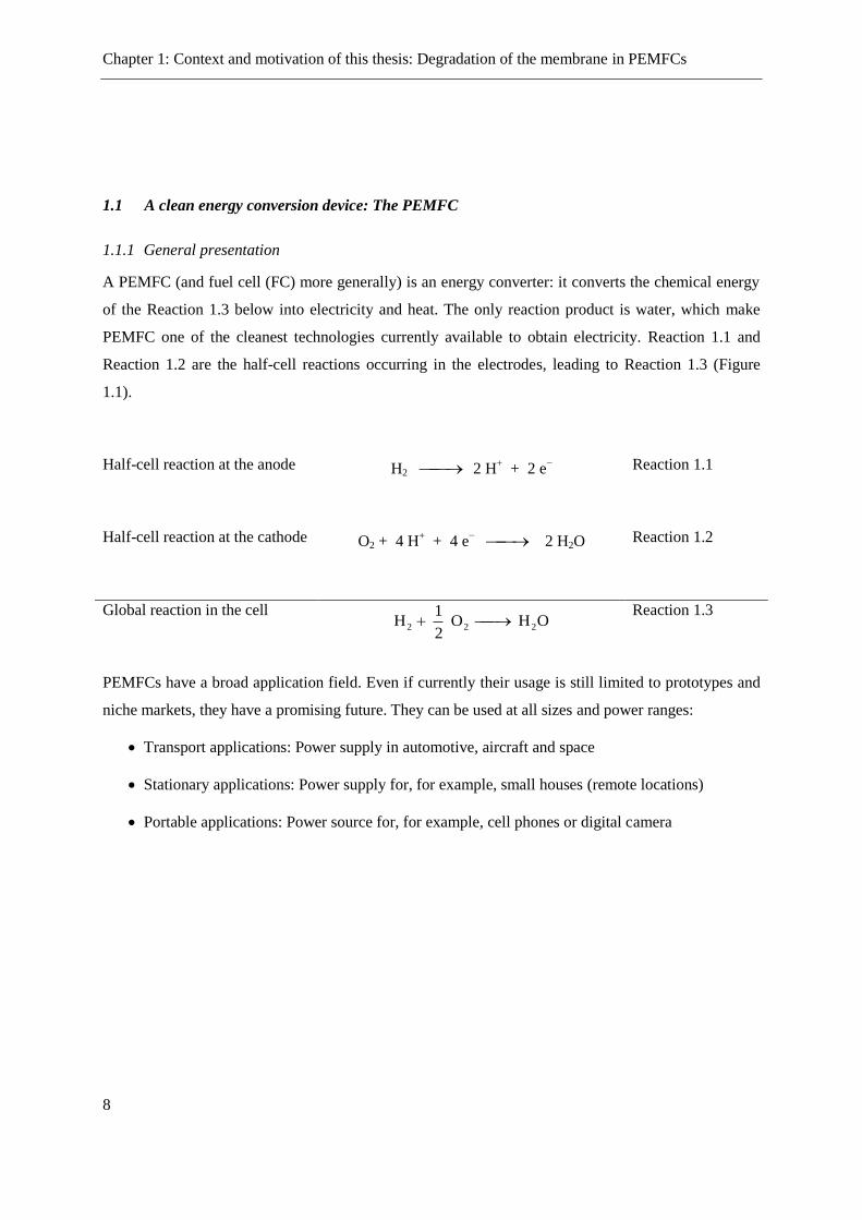
A PEMFC (and fuel cell (FC) more generally) is an energy converter: it converts the chemical energy
of the Reaction 1.3 below into electricity and heat. The only reaction product is water, which make
PEMFC one of the cleanest technologies currently available to obtain electricity. Reaction 1.1 and
Reaction 1.2 are the half-cell reactions occurring in the electrodes, leading to Reaction 1.3 (Figure
1.1).
Half-cell reaction at the anode H2 2 H+ + 2 e
− Reaction 1.1
Half-cell reaction at the cathode O2 + 4 H+ + 4 e
− 2 H2O Reaction 1.2
Global reaction in the cell OH O
2
1 H 222
Reaction 1.3
PEMFCs have a broad application field. Even if currently their usage is still limited to prototypes and
niche markets, they have a promising future. They can be used at all sizes and power ranges:
Transport applications: Power supply in automotive, aircraft and space
Stationary applications: Power supply for, for example, small houses (remote locations)
Portable applications: Power source for, for example, cell phones or digital camera

Chapter 1: Context and motivation of this thesis: Degradation of the membrane in PEMFCs
9
Figure 1.1: Basic diagram of a PEMFC [40]
1.1.2 Components of a PEMFC
Materials and design of a cell are very important because they are the main factors determining the
performance and the life-time of a cell.
We can identify three groups of components in a typical cell:
Components providing a good fuel feed: Bipolar plate and gas diffusion layer (GDL)
Components allowing the reaction of the gases: Electrodes
Component ensuring isolation and proton exchange between the electrodes: Electrolyte (or
membrane)
The combination of the membrane and the electrode is abbreviated under membrane electrode assem-
bly (MEA).
Every component is made of a different material or combination of materials. Table 1.1 summarizes
the different types of material that can be used in the PEMFCs.

Chapter 1: Context and motivation of this thesis: Degradation of the membrane in PEMFCs
10
Component Material Properties
GDL Carbon cloth
Carbon paper
Porous
Electrical conductivity
Bipolar plate Metal
Carbon
Conductive composite polymer
Impermeable to gases
Electrical conductivity
Corrosion resistant
Electrode Catalyst : Platinum and platinum al-
loys supported on carbon black
Ionomer: same material as the corre-
sponding electrolyte
HOR and ORR
Electrical conductivity
Protonic conductivity
Membrane / Elec-
trolyte / Separator
PFSA: Nafion®, Hyflon…
Phosphoric acid doped polybenzimid-
azole (PBI)
Impermeable to gases
High protonic conductivity
Chemical, thermal and me-
chanical stability
Table 1.1: Materials and properties of the PEMFC components
GDLs, whose thickness lies in generally between 100 and 300 µm, have two functions. Firstly they
allow a good diffusion of the gases to the active site in the electrodes and secondly they are one of the
links in the chain of the conduction of electron from the anode to the cathode. Thus they have to be
conductive and porous. Moreover they have a key role in the water management in the membrane
because they must both humidify the membrane and allow water removal (prevention of the water
flooding at the cathode side at high current density).
Bipolar plates are often made of high-density graphite, but gold-coated steel can be for example used
as well. Their main role is the distribution of gases over the whole surface of the electrode and the
conduction of the excess water outside of the system. They are also current collectors. Electrons flow
through the GDL at the anode to the bipolar plate, then go through an external circuit and arrive at the
bipolar plate at the cathode. At a stack level, it is the junction element separating the cathode of a cell
from the anode of the following one. The fluid transport is achieved through micro-channels (width ≈
0.8 mm). The geometry of the channel is very important because it will ensure a homogenous gas sup-
ply in the cell, as it can be seen in Figure 1.2.
Chapter 1: Context and motivation of this thesis: Degradation of the membrane in PEMFCs
11
Figure 1.2: Examples of flow field used at the laboratory scale
In PEMFCs, the electrodes are based on precious metals. These precious metals represent the lightest
part of the whole electrode material but they are the most important because of their catalytic proper-
ties. The most commonly used catalyst is platinum Pt. The amount of Pt in a single cell varies from 0.1
to 1 mg·cm−2
. It could be used under a pure form, but for economic reasons, it is deposited on small
particles of active coal with very high specific area. Their role is to catalyze the hydrogen oxidation
reaction (HOR) (resp. oxygen reduction reaction (ORR)) at the anode (resp. cathode). Electrodes are
very expensive because of the use of Pt (on 2nd
of February 2012 39.50€/g). However, only a small
area of Pt is effectively used (20 % to 30 % of the metal). Therefore efforts are made to control and to
improve the geometry of the electrode structural properties (for example by electrode deposition) [41].
One other area of research is the development of Pt-based alloys in order to reduce the cost without
reducing performances.
The electrolyte is characteristic for each kind of fuel cell. We focus our attention only on the PEMFC
thus we will mention here only its electrolyte. For low-temperature fuel cells, PFSA membranes are
mostly used. The first materials available in the early 60s were sulfonated polystyrene membranes.
These were rapidly replaced from 1966 by Nafion®, developed by the company Du Pont de Nemours,
but over the years many other companies developed their own PFSA membrane (for example Solvay
Solexis, 3M, Gore…). These membranes are ion exchanger. They permit the permeation of cations,
like hydronium ions H3O+ and water can move within the membrane. Another essential function of the
membrane is the separation of the gases to prevent any chemical short circuit (that means ORR and
HOR taking place at the same electrode, in that case electrons will not have to flow through the exter-
nal circuit). Moreover the membrane should not be electrically conductive. PFSA membranes operate

Chapter 1: Context and motivation of this thesis: Degradation of the membrane in PEMFCs
12
up to 90 °C. Above this temperature, other materials have to be used. Indeed water management is a
key challenge for a successful operation of PEMFCs. Above 100 °C, liquid water cannot ensure its
role in proton conduction anymore and thus no proton transport can occur, leading to the failure of the
cell. For High-Temperature PEMFCs (HT-PEM), PBI membranes are used. In these membranes, pro-
ton transport occurs through a rapid proton exchange (hopping mechanism) between phosphate and
amidazole moieties and self-diffusion of phosphate moieties [42].
1.2 Nafion®: The most famous electrolyte for PEMFC
1.2.1 An enigma for modelers and polymer scientists
Nafion® ionomers are developed by the company Du Pont de Nemours since the early 1960s. These
materials are the result of the copolymerization of tetrafluorethylene (TFE, also known as Teflon) with
a perfluorinated vinyl ether comonomer. A common representation for an elementary unit of Nafion®
polymer is given in Figure 1.3. This copolymerization is not well-controlled and there is no clue to
determine if the distribution of the side chain is uniform on the back bone [43, 44]. For this reason, the
concept of equivalent weight (EW) has been introduced. It is defined as the weight of dry Nafion® per
mol of sulfonate acid groups and corresponds to the quantity of polymer needed to neutralize one
equivalent of base. This value is linked to the ion-exchange capacity (IEC) through
IECEW
1000 .
Equation 1.1
The official nomenclature chosen for Nafion® membrane is following: The two first numbers corre-
spond to the EW. For example for Nafion® 112, the EW is 11·100 g·eq
–1, 1100 g/eq. The last number
(in this example 2) corresponds to the membrane thickness in milli-inches (mil). 1 mil represents 25.4
µm, thus Nafion® 112 has a thickness of about 50 µm.
Experimentally the EW can be for example measured by acid-base titration. From the Figure 1.3, we
see that the structure of Nafion® is governed by the choice of 4 indices, determined by the comonomer
chosen during the synthesis. x indicates also how many –CF2- groups are present on the back bone
between two carbon atoms wearing a side chain.
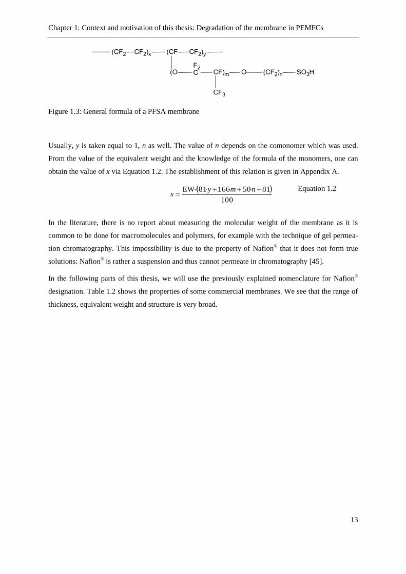
Chapter 1: Context and motivation of this thesis: Degradation of the membrane in PEMFCs
13
Figure 1.3: General formula of a PFSA membrane
Usually, y is taken equal to 1, n as well. The value of n depends on the comonomer which was used.
From the value of the equivalent weight and the knowledge of the formula of the monomers, one can
obtain the value of x via Equation 1.2. The establishment of this relation is given in Appendix A.
100
81·50·166·81EW
nmy-x
Equation 1.2
In the literature, there is no report about measuring the molecular weight of the membrane as it is
common to be done for macromolecules and polymers, for example with the technique of gel permea-
tion chromatography. This impossibility is due to the property of Nafion® that it does not form true
solutions: Nafion® is rather a suspension and thus cannot permeate in chromatography [45].
In the following parts of this thesis, we will use the previously explained nomenclature for Nafion®
designation. Table 1.2 shows the properties of some commercial membranes. We see that the range of
thickness, equivalent weight and structure is very broad.
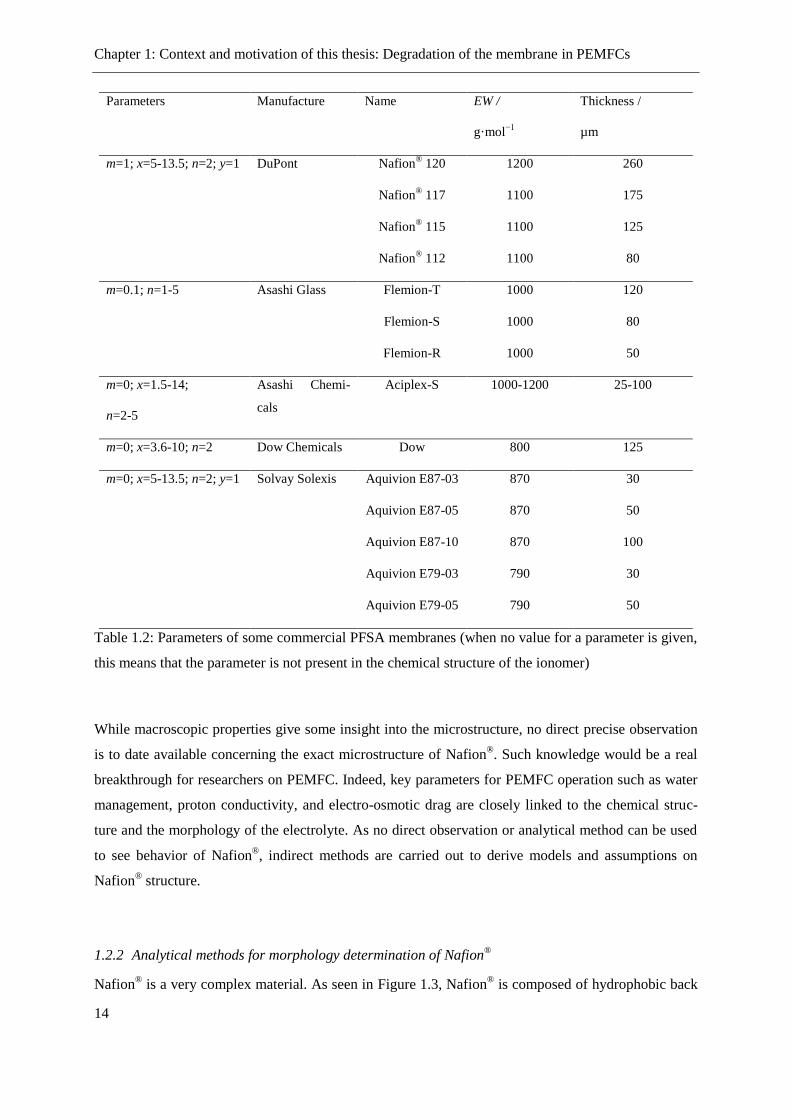
Chapter 1: Context and motivation of this thesis: Degradation of the membrane in PEMFCs
14
Parameters Manufacture Name EW /
g·mol−1
Thickness /
µm
m=1; x=5-13.5; n=2; y=1 DuPont Nafion® 120 1200 260
Nafion® 117 1100 175
Nafion® 115 1100 125
Nafion® 112 1100 80
m=0.1; n=1-5 Asashi Glass Flemion-T 1000 120
Flemion-S 1000 80
Flemion-R 1000 50
m=0; x=1.5-14;
n=2-5
Asashi Chemi-
cals
Aciplex-S 1000-1200 25-100
m=0; x=3.6-10; n=2 Dow Chemicals Dow 800 125
m=0; x=5-13.5; n=2; y=1 Solvay Solexis Aquivion E87-03 870 30
Aquivion E87-05 870 50
Aquivion E87-10 870 100
Aquivion E79-03 790 30
Aquivion E79-05 790 50
Table 1.2: Parameters of some commercial PFSA membranes (when no value for a parameter is given,
this means that the parameter is not present in the chemical structure of the ionomer)
While macroscopic properties give some insight into the microstructure, no direct precise observation
is to date available concerning the exact microstructure of Nafion®. Such knowledge would be a real
breakthrough for researchers on PEMFC. Indeed, key parameters for PEMFC operation such as water
management, proton conductivity, and electro-osmotic drag are closely linked to the chemical struc-
ture and the morphology of the electrolyte. As no direct observation or analytical method can be used
to see behavior of Nafion®, indirect methods are carried out to derive models and assumptions on
Nafion® structure.
1.2.2 Analytical methods for morphology determination of Nafion®
Nafion® is a very complex material. As seen in Figure 1.3, Nafion
® is composed of hydrophobic back
Chapter 1: Context and motivation of this thesis: Degradation of the membrane in PEMFCs
15
bones (Teflon skeleton) and hydrophilic side chains (the ionic sulfonate head). Thus the study of the
morphology of Nafion® has to be done in regards to the water content in the membrane.
Many analytical methods have been used to analyze structural properties of Nafion®, but scientists
always kept in mind that their conclusions about the structure of Nafion® are relevant only if they are
put into correlation with the hydration of the membrane.
The first step after having synthesized a new material is its characterization. The molecular formula
can be determined by nuclear magnetic resonance (NMR). In the case of Nafion®, such measurements
were presented in the literature [46-49]. This technique is used since the beginning of the 80s to de-
termine the molecular structure of synthesized Nafion® [47]. NMR allows knowing which atom
groups are located in the molecule and which groups are locate in their vicinity. In fact, the structure
of Nafion® was assumed knowing the comonomer and the Teflon structure, and, NMR confirmed the
molecular formula. This technique is still not sufficient to advance conclusions about the morphologi-
cal structure of this polymer.
A powerful technique to inquire indirectly through Nafion® is the uses of X-rays and neutrons. This
technique is since the 70s one of the most used to study Nafion®. Such measurements were carried out
under every possible experimental condition [11, 50-54]. But it is here neither the purpose to present
an exhaustive list of the every paper dealing with small-angle X-ray scattering (SAXS), small-angle
neutron scattering (SANS) and wide-angle X-ray diffraction (WAXD) nor detailing these very com-
plex analytical methods.
We rather focus on some of the most cited and recognized papers which offered new insights and pro-
posals about the Nafion® structure.
Gierke et al. were one of the pioneer researchers in this field [10]. He examined and compared the
morphological features of Nafion®, having a range of EW, in the unhydrolyzed sulfonyl fluoride pre-
cursor form, the hydrolyzed sulfonyl acid form and the neutralized metal sulfonate form. From SAXS
experiment they observed evidences for crystalline structure within the fluorocarbon matrix. With a
hydrolyzed form of Nafion®, they found evidences characteristic of a system containing ionic clusters
within a semicrystalline matrix [55]. Based on further SAXS and WAXD analysis with the observa-
tion of two scattering peaks on the profiles and considering the three most prevalent models for the
morphology of ionomers at the time, including a model of spherical clusters on a paracrystalline lat-
tice, a core-shell model, and a lamellar model, Gierke and co-workers concluded that the water-
swollen morphology of Nafion® was best described by a model of ionic clusters that were approxi-
mately spherical in shape with an inverted micellar structure [10, 56]. In consideration of the high
ionic permselectivity and the requirement of a percolation pathway for ionic transport in Nafion®
membranes, the spherical ionic clusters were further proposed to be interconnected by narrow chan-

Chapter 1: Context and motivation of this thesis: Degradation of the membrane in PEMFCs
16
nels, constituting a morphology referred to as the cluster-network model as displayed Figure 1.4 [57,
58].
Figure 1.4: Cluster-network model from Gierke [59].
Fujimura et al. performed SAXS and WAXD experiments as well in order to define the morphological
origins of the two scattering peaks. In order to analyze the effect of ionic interactions due to the side
chain, they neutralized chemically the sulfonated groups of the side chain into sulfonyl chloride, simi-
lar to Nafion® but nonionic [60, 61]. Like Gierke, Fujimura found two scattering maxima at s = 0.07
nm and 0.3 nm−1
(s is scattering vector, defined as s= 2·sin(θ) / λ) which were attributed to crystalline
and ionic domains. They also concluded from their measurements that the crystallinity of a Nafion®
whose EW is 1100 g·mol−1
was 23% and 18-14% crystalline in the nonionic and carboxylated forms,
respectively. The low angle scattering maximum at s = 0.07 nm−1
was supposed to be an average spac-
ing between crystalline lamellar plate. At higher humidification, the cluster dimension is shown to
increase. Fujimura et al concluded that the observed behavior can be the best described by an intra-
particle core-shell model [60]. A schematically representation is given in Figure 1.5.
Figure 1.5: Modified core-shell model for Nafion® [60].

Chapter 1: Context and motivation of this thesis: Degradation of the membrane in PEMFCs
17
Haubold et al. proposed a variation of the lamellar model of Litt as presented in Figure 1.6 [11, 62].
They performed SAXS studies for that. They observed the usual peak at 1.4 nm−1
. The scattering cross
section data was fitted to a layered model whose structure element is a “sandwich”. The outer portion
(shell) is composed by the side chains and the core is a liquid phase with water (and methanol in their
case – Direct Methanol Fuel Cell (DMFC) conditions). In order to provide channels for the proton
transport along the membrane, the “sandwiches” were stacked in a linear fashion so that the liquid core
regions are contiguous as shown in Figure 1.7 [58].
Figure 1.6: Haubold's sandwich-like structure for Nafion® [11]

Chapter 1: Context and motivation of this thesis: Degradation of the membrane in PEMFCs
18
Figure 1.7: Stack of element to describe proton conductivity in Nafion® [11]
Most of these models regard fully-humidified membranes. Gebel proposed a conceptual description
for the swelling and dissolution process, as shown in Figure 1.8. In this qualitative model, the dry
membrane is considered to contain isolated, spherical ionic clusters with diameters of 1.5 nm and a
center-to-center separation distance of 2.7 nm. With the absorption of water, the clusters swell to hold
pools of water surrounded by ionic groups at the polymer water interface in order to minimize the
interfacial energy. As the water content increases to a water volume fraction between 0.3 and 0.5,
structural reorganization occurs to keep constant the specific surface area, and the onset of percolation
is achieved by the formation of connecting cylinders of water between the swollen, spherical clusters.
At water volume fraction values greater than 0.5, an inversion of the structure occurs such that the
structure resembles a connected network of rods (inverted micelles). Finally, as the membrane “dis-
solves” into solution, the rodlike structures separate to yield a colloidal dispersion of isolated rods
[58].

Chapter 1: Context and motivation of this thesis: Degradation of the membrane in PEMFCs
19
Figure 1.8: Schematic evolution of the Nafion® structure depending on the water content [63]
In the continuity of this work, Rubatat et al combined neutron and X-ray scattering techniques, and
extended the range of X-ray scattering by using Ultra SAXS [12]. They collected scattering data from
Nafion® samples at various water contents. Maxima positions and shapes of scattering profiles were
similar to what other groups previously reported in the literature. This observation supported the as-
sumption that the swelling process involves a dilution of the scattering entities, and not a strong struc-
tural reorganization as previously proposed [63]. This dissociation was partial and continuous over the
whole swelling process [64]. Although the real description should be more complex, the assumption of
Rubatat that the Nafion® membrane was composed of an assembly of bundles of fibrils (as displayed
in Figure 1.9) allowed them to analyze the anisotropic scattering spectra observed when a strain is
applied on the membrane. They assumed the morphology of Nafion® as a mixture between amorphous
phases and ordered phases, whose dimensions were derived from USAXS and organization by the
ionomer peak on measured profiles.

Chapter 1: Context and motivation of this thesis: Degradation of the membrane in PEMFCs
20
Figure 1.9: Schematic view of correlated polymeric aggregates domains [65]
Weber and Newman treated the Hsu and Gierke cluster-network model as an idealization of the
Yeager and Steck model, where the pathways between the clusters are the interfacial regions [14, 57,
66]. The main focus of the model is how the membrane structure changes as a function of water con-
tent, where λ is the moles of water per mole of sulfonic acid sites (Figure 1.10). In the first step, the
dry membrane absorbs water in order to solvate the acid groups. The initial water is associated strong-
ly with the sites, and with the addition of more water in the membrane, the water becomes less bound,
and inverted micelles form in the polymer matrix. With more water uptake, these clusters grow and
form interconnections with each other. The connections, or collapsed channels, are transitory and have
hydrophobicities comparable to the matrix. The cluster-channel network forms based on a percolation-
type phenomenon of the clusters; therefore, to form a transport pathway, the clusters must grow and be
close enough together to be linked by the collapsed channels [67].
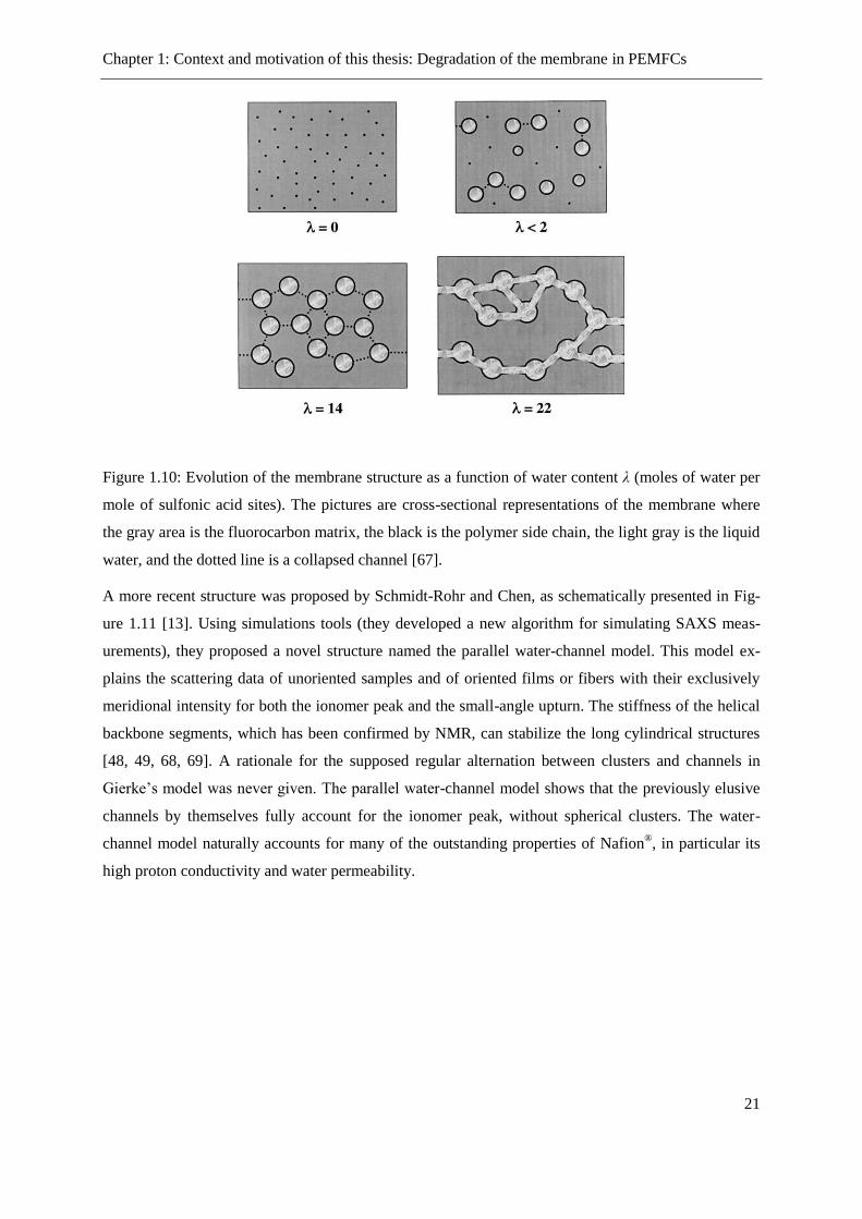
Chapter 1: Context and motivation of this thesis: Degradation of the membrane in PEMFCs
21
Figure 1.10: Evolution of the membrane structure as a function of water content λ (moles of water per
mole of sulfonic acid sites). The pictures are cross-sectional representations of the membrane where
the gray area is the fluorocarbon matrix, the black is the polymer side chain, the light gray is the liquid
water, and the dotted line is a collapsed channel [67].
A more recent structure was proposed by Schmidt-Rohr and Chen, as schematically presented in Fig-
ure 1.11 [13]. Using simulations tools (they developed a new algorithm for simulating SAXS meas-
urements), they proposed a novel structure named the parallel water-channel model. This model ex-
plains the scattering data of unoriented samples and of oriented films or fibers with their exclusively
meridional intensity for both the ionomer peak and the small-angle upturn. The stiffness of the helical
backbone segments, which has been confirmed by NMR, can stabilize the long cylindrical structures
[48, 49, 68, 69]. A rationale for the supposed regular alternation between clusters and channels in
Gierke’s model was never given. The parallel water-channel model shows that the previously elusive
channels by themselves fully account for the ionomer peak, without spherical clusters. The water-
channel model naturally accounts for many of the outstanding properties of Nafion®, in particular its
high proton conductivity and water permeability.
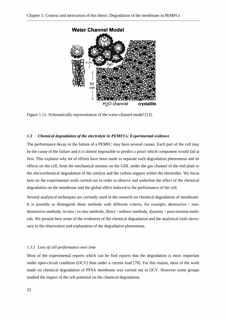
Chapter 1: Context and motivation of this thesis: Degradation of the membrane in PEMFCs
22
Figure 1.11: Schematically representation of the water-channel model [13].
1.3 Chemical degradation of the electrolyte in PEMFCs: Experimental evidence
The performance decay or the failure of a PEMFC may have several causes. Each part of the cell may
be the cause of the failure and it is almost impossible to predict a priori which component would fail at
first. This explains why lot of efforts have been made to separate each degradation phenomena and its
effects on the cell, from the mechanical stresses on the GDL under the gas channel of the end plate to
the electrochemical degradation of the catalyst and the carbon support within the electrodes. We focus
here on the experimental work carried out in order to observe and underline the effect of the chemical
degradation on the membrane and the global effect induced to the performance of the cell.
Several analytical techniques are currently used in the research on chemical degradation of membrane.
It is possible to distinguish these methods with different criteria, for example, destructive / non-
destructive methods, in-situ / ex-situ methods, direct / indirect methods, dynamic / post-mortem meth-
ods. We present here some of the evidences of the chemical degradation and the analytical tools neces-
sary to the observation and explanation of the degradation phenomena.
1.3.1 Loss of cell performance over time
Most of the experimental reports which can be find reports that the degradation is more important
under open-circuit condition (OCV) than under a current load [70]. For this reason, most of the work
made on chemical degradation of PFSA membrane was carried out at OCV. However some groups
studied the impact of the cell potential on the chemical degradation.
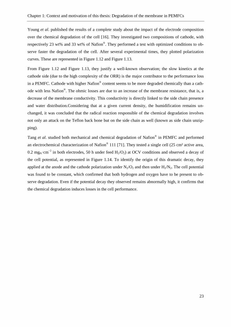
Chapter 1: Context and motivation of this thesis: Degradation of the membrane in PEMFCs
23
Young et al. published the results of a complete study about the impact of the electrode composition
over the chemical degradation of the cell [16]. They investigated two compositions of cathode, with
respectively 23 wt% and 33 wt% of Nafion®. They performed a test with optimized conditions to ob-
serve faster the degradation of the cell. After several experimental times, they plotted polarization
curves. These are represented in Figure 1.12 and Figure 1.13.
From Figure 1.12 and Figure 1.13, they justify a well-known observation; the slow kinetics at the
cathode side (due to the high complexity of the ORR) is the major contributor to the performance loss
in a PEMFC. Cathode with higher Nafion® content seems to be more degraded chemically than a cath-
ode with less Nafion®. The ohmic losses are due to an increase of the membrane resistance, that is, a
decrease of the membrane conductivity. This conductivity is directly linked to the side chain presence
and water distribution.Considering that at a given current density, the humidification remains un-
changed, it was concluded that the radical reaction responsible of the chemical degradation involves
not only an attack on the Teflon back bone but on the side chain as well (known as side chain unzip-
ping).
Tang et al. studied both mechanical and chemical degradation of Nafion® in PEMFC and performed
an electrochemical characterization of Nafion® 111 [71]. They tested a single cell (25 cm² active area,
0.2 mgPt·cm−2
in both electrodes, 50 h under feed H2/O2) at OCV conditions and observed a decay of
the cell potential, as represented in Figure 1.14. To identify the origin of this dramatic decay, they
applied at the anode and the cathode polarization under N2/O2 and then under H2/N2. The cell potential
was found to be constant, which confirmed that both hydrogen and oxygen have to be present to ob-
serve degradation. Even if the potential decay they observed remains abnormally high, it confirms that
the chemical degradation induces losses in the cell performance.

Chapter 1: Context and motivation of this thesis: Degradation of the membrane in PEMFCs
24
Figure 1.12: IV-curve (a) 23 wt% Nafion® in
cathode and repartition of losses (b) at 2.5
A·cm−2
taken at () 0, (♦) 150, ()300, and (x)
440 h [16]
Figure 1.13: IV-curve (a) 33 wt% Nafion® in
cathode and repartition of losses (b) at 2.5
A·cm−2
taken at () 0, (♦) 150, ()300, and
(x)440 h [16]

Chapter 1: Context and motivation of this thesis: Degradation of the membrane in PEMFCs
25
Figure 1.14: Evolution of the cell potential under OCV conditions [71].
Similar behavior was observed by Inaba et al. [72]. The potential loss is not so large than in the exper-
iment of Tang but a decrease is observed. In Figure 1.15, we can see at the OCV, the potential is de-
creasing. This potential loss is to be compared with the temporal evolution of the hydrogen crossover
from the anode to the cathode (Figure 1.16).
Figure 1.15: Variation of the open-circuit voltage of H2/air cell during OCV durability test at 80 °C
[72].
Chapter 1: Context and motivation of this thesis: Degradation of the membrane in PEMFCs
26
Figure 1.16: Variation of the H2 crossover current density during OCV durability test at 80 °C [72].
At every 24 h, air was replaced with argon to measure hydrogen crossover current, where the OCV
dropped down to about 100 mV in. In each 24 h, the OCV was the highest just after air was introduced
in the cell, and then dropped gradually with time. This phenomenon is attributed by the authors to
reversible oxide film formation on the cathode Pt catalyst and hence is a reversible degradation phe-
nomenon. The OCV (just after air was introduced at every 24 h) slowly decreased to about 840 mV
after 60 days. The average voltage degradation rate was ca. 83 µV·h−1
, which is much faster than that
in normal operation (a few to several µV·h−1
) under fully humidified conditions. Consequently, the
open-circuit condition accelerates the degradation of the MEA [72].
Based on the work of Young et al., the performance loss remains low compared for example to ohmic
losses due to the degradation of the carbon catalyst support [16]. Schulze et al. analyzed the effect of
degradation on a fuel cell and observed through electrochemical impedance spectroscopy (EIS) meas-
urement an increase of the carbon-support resistance of about 14 mΩ, whereas the increase of the
membrane resistance was barely measurable [73]. However, the degradation strongly depends on the
experimental conditions, materials and cell design (e.g. channels geometry) used.
1.3.2 Membrane thinning
As the loss in performance is not a reliable tool to quantify and identify the chemical degradation of
the membrane, experimentalists had to find other ways to characterize the chemical degradation of
Nafion®. The chemical degradation “removes” atoms from the membrane, thus we can expect that the
membrane slowly vanishes into the liquid phase. An effect would then be the decrease of the mem-
brane thickness. The most common way to observe it is the use of high resolution microscopes.

Chapter 1: Context and motivation of this thesis: Degradation of the membrane in PEMFCs
27
Tang et al. put the membranes into bottles under conditions of dry, atmospheric humidity, saturated
humidity and 1 mol·l−1
H2SO4 [71]. These bottles were then fed with 100 sccm H2 and 100 sccm O2
respectively. They measured the membrane thickness after 1000 h in different operations conditions
that would exist in the fuel cell. Table 1.3 sums up the result of these measurements
Thickness / µm
Original Nafion®111 25.4 ±0.1
1000 h H2
Absolute dry 25.1 ±0.1
Atmospheric humidity 24.8 ±0.1
100 % RH 25.2 ±0.1
Acidic condition 24.3 ±0.1
With Fe2+
22.4 ±0.1
1000 h O2
Absolute dry 25.2 ±0.1
Atmospheric humidity 24.3 ±0.1
100 % RH 24.2 ±0.1
Acidic condition 23.9 ±0.1
With Fe2+
23.4 ±0.1
Table 1.3: Evolution of membrane thickness of Nafion® membranes exposed in H2 or O2 for 1000 h
(after [71])
They noticed no significant decrease of Nafion® thickness. This indicated that the Nafion
® membrane
is chemically stable vis-a-vis oxygen and hydrogen. This means that the chemical degradation occurs
only in presence of both gases, which was already suggested by the OCV electrochemical experi-
ments.
Healy et al. presented an interesting overview of PFSA chemical degradation in fuel cell utilization
[15]. They performed in-situ and ex-situ experiments in order to understand better the origin of the
degradation. In their investigation, they ran a fuel cell over 1000 h and followed the release of fluoride
ions in drain water, an important by-product of the chemical degradation. They correlated a high fluo-
ride production with a decrease of the membrane thickness. They observed it by comparison of elec-
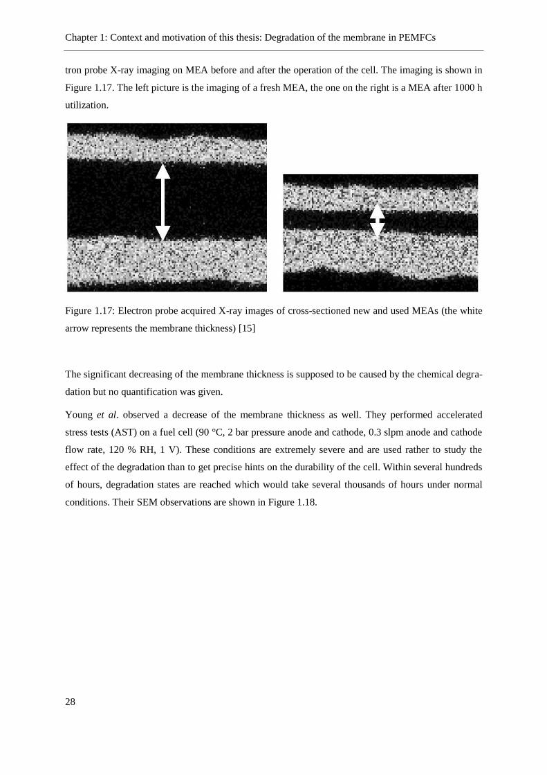
Chapter 1: Context and motivation of this thesis: Degradation of the membrane in PEMFCs
28
tron probe X-ray imaging on MEA before and after the operation of the cell. The imaging is shown in
Figure 1.17. The left picture is the imaging of a fresh MEA, the one on the right is a MEA after 1000 h
utilization.
Figure 1.17: Electron probe acquired X-ray images of cross-sectioned new and used MEAs (the white
arrow represents the membrane thickness) [15]
The significant decreasing of the membrane thickness is supposed to be caused by the chemical degra-
dation but no quantification was given.
Young et al. observed a decrease of the membrane thickness as well. They performed accelerated
stress tests (AST) on a fuel cell (90 °C, 2 bar pressure anode and cathode, 0.3 slpm anode and cathode
flow rate, 120 % RH, 1 V). These conditions are extremely severe and are used rather to study the
effect of the degradation than to get precise hints on the durability of the cell. Within several hundreds
of hours, degradation states are reached which would take several thousands of hours under normal
conditions. Their SEM observations are shown in Figure 1.18.
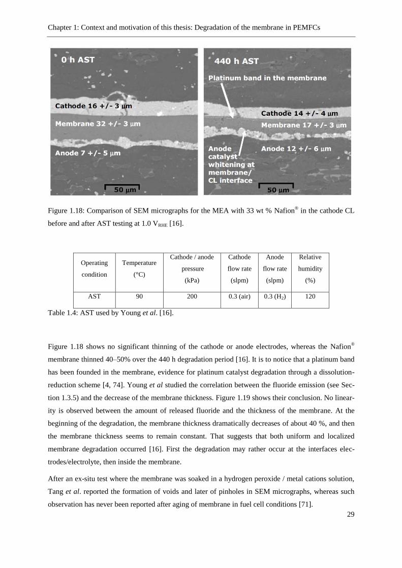
Chapter 1: Context and motivation of this thesis: Degradation of the membrane in PEMFCs
29
Figure 1.18: Comparison of SEM micrographs for the MEA with 33 wt % Nafion® in the cathode CL
before and after AST testing at 1.0 VRHE [16].
Operating
condition
Temperature
(°C)
Cathode / anode
pressure
(kPa)
Cathode
flow rate
(slpm)
Anode
flow rate
(slpm)
Relative
humidity
(%)
AST 90 200 0.3 (air) 0.3 (H2) 120
Table 1.4: AST used by Young et al. [16].
Figure 1.18 shows no significant thinning of the cathode or anode electrodes, whereas the Nafion®
membrane thinned 40–50% over the 440 h degradation period [16]. It is to notice that a platinum band
has been founded in the membrane, evidence for platinum catalyst degradation through a dissolution-
reduction scheme [4, 74]. Young et al studied the correlation between the fluoride emission (see Sec-
tion 1.3.5) and the decrease of the membrane thickness. Figure 1.19 shows their conclusion. No linear-
ity is observed between the amount of released fluoride and the thickness of the membrane. At the
beginning of the degradation, the membrane thickness dramatically decreases of about 40 %, and then
the membrane thickness seems to remain constant. That suggests that both uniform and localized
membrane degradation occurred [16]. First the degradation may rather occur at the interfaces elec-
trodes/electrolyte, then inside the membrane.
After an ex-situ test where the membrane was soaked in a hydrogen peroxide / metal cations solution,
Tang et al. reported the formation of voids and later of pinholes in SEM micrographs, whereas such
observation has never been reported after aging of membrane in fuel cell conditions [71].
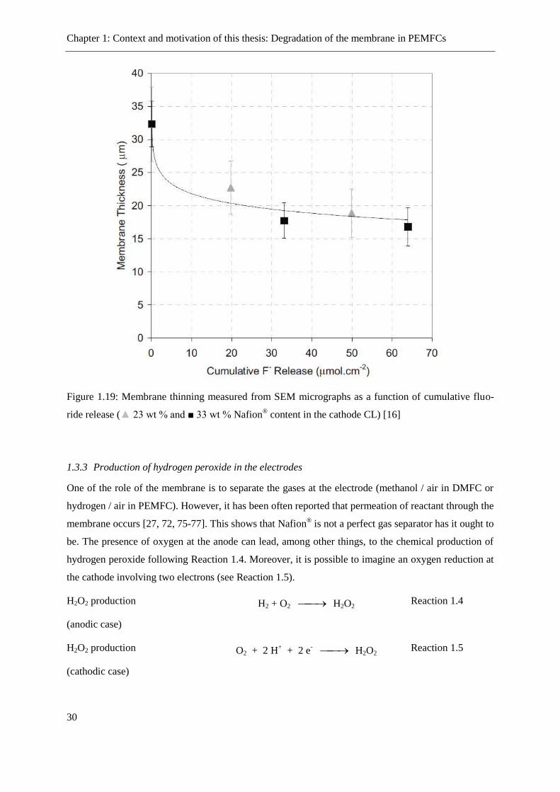
Chapter 1: Context and motivation of this thesis: Degradation of the membrane in PEMFCs
30
Figure 1.19: Membrane thinning measured from SEM micrographs as a function of cumulative fluo-
ride release ( 23 wt % and 33 wt % Nafion® content in the cathode CL) [16]
1.3.3 Production of hydrogen peroxide in the electrodes
One of the role of the membrane is to separate the gases at the electrode (methanol / air in DMFC or
hydrogen / air in PEMFC). However, it has been often reported that permeation of reactant through the
membrane occurs [27, 72, 75-77]. This shows that Nafion® is not a perfect gas separator has it ought to
be. The presence of oxygen at the anode can lead, among other things, to the chemical production of
hydrogen peroxide following Reaction 1.4. Moreover, it is possible to imagine an oxygen reduction at
the cathode involving two electrons (see Reaction 1.5).
H2O2 production
(anodic case)
H2 + O2 H2O2 Reaction 1.4
H2O2 production
(cathodic case)
O2 + 2 H+ + 2 e
- H2O2 Reaction 1.5

Chapter 1: Context and motivation of this thesis: Degradation of the membrane in PEMFCs
31
However there is still debate in the literature to see if the major location of H2O2 production is at the
anode or the cathode side [17, 18, 78]. The understanding of ORR mechanism was already experimen-
tally studied by Davies et al. and Yeager [79-83]. Davies et al. proposed several mechanisms for the
oxygen reduction in their study on the oxygen electrode in 1959 [79]. They proposed three possible
mechanisms for this reaction on carbon in alkaline solution as shown in Figure 1.20 In a modern
PEMFC, the pH of the cell is strongly acidic. But we could assume that the mechanism is not deeply
influenced as basic species appear on the product side of the reactions. Yeager studied the oxygen
reduction reaction on several surfaces [82]. In our case, the surfaces of interest are platinum and car-
bon, as they are the active constituents of the considered electrodes. Using the rotating ring-disc elec-
trode (RRDE) technique on Pt, they get evidence that the O2 reduction is carried out principally
through the 4-electron pathway in both acid and alkaline aqueous electrolytes under conditions where
adsorbed impurities are minimal. However on his study on graphite and carbon he considered peroxide
as a possible intermediate in the ORR, a mechanism was published by Morcos et al. [81].
Figure 1.20: Oxygen reduction on carbon under alkaline conditions [79].
Ab initio calculations, within the Density Functional Theory -DFT- approach, are also carried out to
elucidate ORR mechanism on different catalysts and the different pathways leading to H2O2 formation
[84-88].
Mittal et al. showed that hydrogen peroxide is formed in PEMFC [78]. They could not answer the
question whether the production occurs at the anode or the cathode because of diffusing effects in the
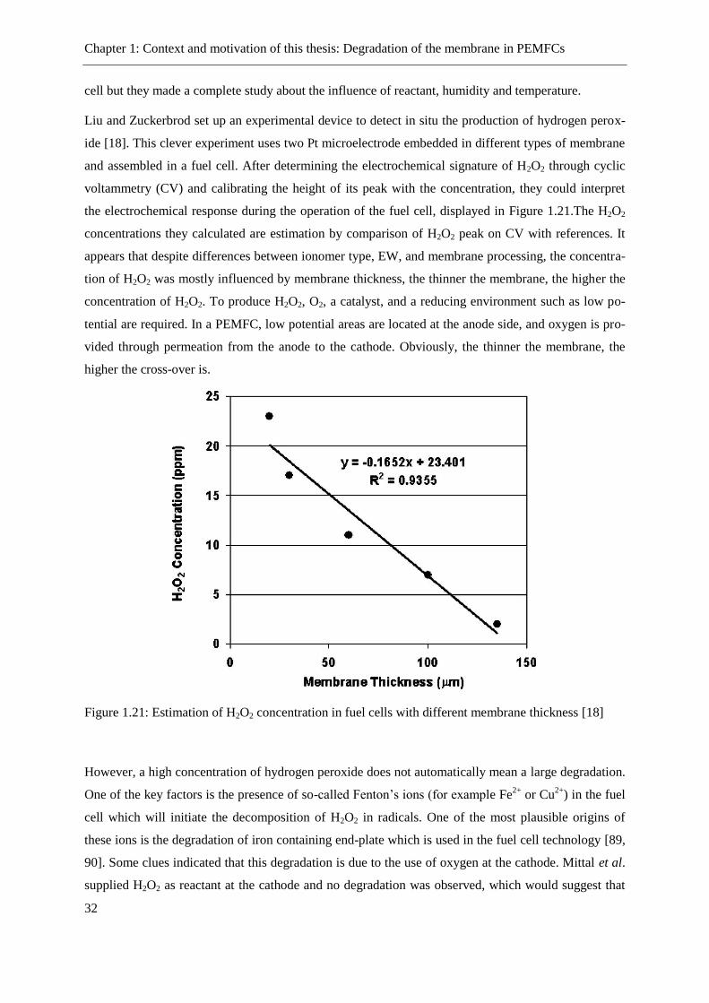
Chapter 1: Context and motivation of this thesis: Degradation of the membrane in PEMFCs
32
cell but they made a complete study about the influence of reactant, humidity and temperature.
Liu and Zuckerbrod set up an experimental device to detect in situ the production of hydrogen perox-
ide [18]. This clever experiment uses two Pt microelectrode embedded in different types of membrane
and assembled in a fuel cell. After determining the electrochemical signature of H2O2 through cyclic
voltammetry (CV) and calibrating the height of its peak with the concentration, they could interpret
the electrochemical response during the operation of the fuel cell, displayed in Figure 1.21.The H2O2
concentrations they calculated are estimation by comparison of H2O2 peak on CV with references. It
appears that despite differences between ionomer type, EW, and membrane processing, the concentra-
tion of H2O2 was mostly influenced by membrane thickness, the thinner the membrane, the higher the
concentration of H2O2. To produce H2O2, O2, a catalyst, and a reducing environment such as low po-
tential are required. In a PEMFC, low potential areas are located at the anode side, and oxygen is pro-
vided through permeation from the anode to the cathode. Obviously, the thinner the membrane, the
higher the cross-over is.
Figure 1.21: Estimation of H2O2 concentration in fuel cells with different membrane thickness [18]
However, a high concentration of hydrogen peroxide does not automatically mean a large degradation.
One of the key factors is the presence of so-called Fenton’s ions (for example Fe2+
or Cu2+
) in the fuel
cell which will initiate the decomposition of H2O2 in radicals. One of the most plausible origins of
these ions is the degradation of iron containing end-plate which is used in the fuel cell technology [89,
90]. Some clues indicated that this degradation is due to the use of oxygen at the cathode. Mittal et al.
supplied H2O2 as reactant at the cathode and no degradation was observed, which would suggest that

Chapter 1: Context and motivation of this thesis: Degradation of the membrane in PEMFCs
33
no iron was produced in the system [78].
1.3.4 Formation of radicals
Hydroxyl radicals are highly reactive and consequently short-lived. They are really difficult to be ob-
served because of their low life-time (about 10−9
s). Two solutions may be envisaged to solve this
problem: trapping the radical under a more stable form or cool down (77 K) the membrane to make
direct observations.
Aoki et al. used 5,5’-dimethyl-1-pyrroline-N-oxide (DMPO) was added in a H2O2 solution suspending
various types of membrane as a spin trap reagent to form DMPO-OH adduct [91]. After 5 min, they
then measured by electron spin resonance (ESR), technique also known as electronic paramagnetic
resonance (EPR) the amount of hydroxyl radical which has been produced. Figure 1.22 shows the
amount measured under several conditions.
Figure 1.22: Hydroxyl radical generated in membrane in different solutions [91]
The essential role of ferrous iron is here confirmed. A self-decomposition of H2O2 is really low. But
the presence of Fe2+
increases the amount of produced hydroxyl radicals.
Panchenko et al. developed a cell capable of operating in the resonator of an X-band EPR-
spectrometer [92]. This method was used by Vogel et al. to observe in-situ formation of radical during
the operation of a fuel cell [93]. They concluded to the role of hydroxyl radicals in the attack of mem-
brane.

Chapter 1: Context and motivation of this thesis: Degradation of the membrane in PEMFCs
34
Kadirov et al. analyzed by ESR membrane neutralized with different metal cations (Cu2+
, Fe2+
, Fe3+
)
[28]. Their measurement at 77 K lead to the conclusion that the presence of Fe2+
, Fe3+
, or Cu2+
in com-
bination with hydrogen peroxide and UV irradiation leads to extensive radical formation on PFSA
membranes.
Danilczuk et al. performed in situ ESR measurement of a PEMFC at 300 K [27]. They concluded that
the production of hydrogen peroxide (and thus of radicals) occurred at the cathode side only in closed
circuit voltage (CCV), which suggests an electrochemical production of hydrogen peroxide through a
two electron reduction step of oxygen in these conditions. However the possibility of a radical produc-
tion at the anode is not excluded [18, 94-96].
1.3.5 Chemical analysis of the degradation of PFSA membranes
The most reported method to underline the PFSA membrane degradation is the measurement of fluo-
ride ions (fluoride emission rate FER) in the drain water of the cell. One of the products of the degra-
dation of Nafion® is fluoride ions. As the initial conditions of a cell do not include the presence of
fluoride in ionic form, their presence in the drain water is a direct measure of the chemical degrada-
tion. Many analytical methods have been developed to measure the quantity of fluoride in the pro-
duced water or on the contrary, the remaining fluoride in the membrane.
Healy et al. found through 19
F NMR a fluoride peak in the drain water (water which leaves the system
through the gas channels) of a severely degraded membrane which was not present in an unused MEA
[15]. It was assigned to perfluoro(3-oxapentane)-1-sulfonic-4-carboxylic diacid (later named molecule
A) displayed in Figure 1.23. This was confirmed by mass spectrometry (MS). This molecule is a sort
of acidic form of side chain, resulting of the side chain unzipping during degradation.
Figure 1.23: Semi-developed formula of perfluoro(3-oxapentane)-1-sulfonic-4-carboxylic diacid (mol-
ecule A)

Chapter 1: Context and motivation of this thesis: Degradation of the membrane in PEMFCs
35
The total amount of fluoride ions which have been released has been determined through ionic chro-
matography. The amount of fluoride is a parameter which should not linearly assimiled to the rate of
degradation of the membrane. Indeed it strongly depends to the experimental conditions, the amount
of produced hydrogen peroxide, the presence of iron ions, membrane thickness and a part of the de-
graded fluoride may remain under organic form [15, 16, 37, 72, 97-99]. Thus experimental results are
very difficult to be interpreted.
Another possibility is to follow the evolution of the mass of the membrane [100]. Kundu et al. per-
formed two accelerated degradation test and compared them. The first method exposes the membrane
to a solution of peroxide and metal ions (solution method) while the second method exchanges the
metal ions with the acid sites of the polymer before exposure to peroxide (exchange method) [15, 97].
They started from different iron ions concentrations in the cell and measured the weight loss after a
certain period of degradation. It seemed that the mass loss is independent of the quantity of iron ions,
as after the same periods of time the same mass loss had been observed. However the amount of fluo-
ride produced was different, which was due to the fact that organic fragment of Nafion® remained in
the membrane in one case and could not be then observed by anorganic fluoride sensitive analytic
methods. They found out, depending on the degradation test they used, that the loss of weight lays by
25 % after 120 h, when the amount of fluoride loss was only 0.5 % to 1.5 % of the total amount of
fluoride.
All of these experimental observations are specifically to a single experiment, as some experimental
cannot be controlled (ratio between organic fluoride in degraded products to anorganic fluoride for
example). This explains why experimental works are sometimes linked to a specific model. The next
part deals with relevant modeling work currently available in the literature.
1.4 Chemical degradation of the electrolyte in PEMFCs: Available modeling work
Modeling is a broad field and several works are available in the existing literature. Some of them in-
quire through atomistic calculations the pathways of the chemical degradation; other uses continuum
approaches to make predictions on the behavior the fuel cell or the membrane.
First of all, it is important to know the chemical pathway leading to the chemical degradation of the
membrane. Indeed, no model can be effective if the phenomenon is not perfectly clearly defined. Xie
and Hayden proposed a mechanism of membrane degradation, which is now regarded as the most
plausible approach, exhibing good agreement with experimental works [32].The highly reactive radi-
cal species produced after the permeation of oxygen to the anode side may either react following one
of the reactions described in Section 2.3.1 (Reaction 2.3, Reaction 2.4 and Reaction 2.5) or attack the

Chapter 1: Context and motivation of this thesis: Degradation of the membrane in PEMFCs
36
PFSA membrane.
Figure 1.24: Individual degradation reaction steps via end group unzipping [32]
The carboxylic acid groups present in the membrane are either a direct by-product of the synthesis of
the membrane or the result of reactions of others weak groups (for example –CH2F) with radical spe-
cies. This carboxylic acid reacts with two radicals and through this step, carbon dioxide and HF are
released and the carboxylic acid group is transformed into a fluoride acid group which is then hydro-
lyzed, releasing another HF molecule and regenerating the carboxylic acid group. After each degrada-
tion process, the membrane back bone is reduced by one carbon atom.
During the degradation process it occurs that the carboxylic acid group is located in α of a carbon atom
supporting a side chain. In such a case, we have to consider a parallel degradation pathway, as pre-
sented by Xie and Hayden [32].
Figure 1.25: Secondary degradation reaction via end group unzipping [32].
As mentioned previously in Section 1.3.5, the organic molecule resulting from the unzipping of a side
chain is called molecule “A” in order to simplify the discussion, as shown in Figure 1.25. This mole-
cule A has been observed experimentally thus confirming this parallel process [15]. The molecule A
can itself be degraded under radical attack and be decomposed into HF, CO2 and sulfate ions, as
shown in Figure 1.26.
Molecule A
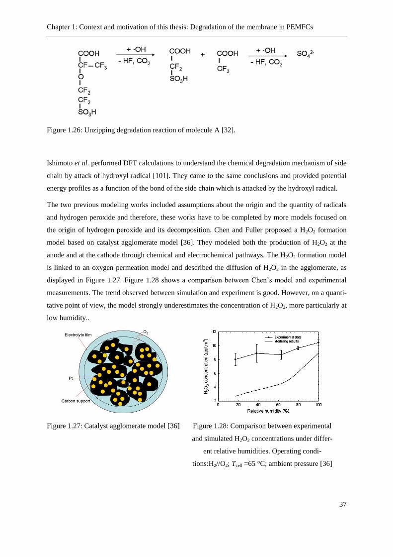
Chapter 1: Context and motivation of this thesis: Degradation of the membrane in PEMFCs
37
Figure 1.26: Unzipping degradation reaction of molecule A [32].
Ishimoto et al. performed DFT calculations to understand the chemical degradation mechanism of side
chain by attack of hydroxyl radical [101]. They came to the same conclusions and provided potential
energy profiles as a function of the bond of the side chain which is attacked by the hydroxyl radical.
The two previous modeling works included assumptions about the origin and the quantity of radicals
and hydrogen peroxide and therefore, these works have to be completed by more models focused on
the origin of hydrogen peroxide and its decomposition. Chen and Fuller proposed a H2O2 formation
model based on catalyst agglomerate model [36]. They modeled both the production of H2O2 at the
anode and at the cathode through chemical and electrochemical pathways. The H2O2 formation model
is linked to an oxygen permeation model and described the diffusion of H2O2 in the agglomerate, as
displayed in Figure 1.27. Figure 1.28 shows a comparison between Chen’s model and experimental
measurements. The trend observed between simulation and experiment is good. However, on a quanti-
tative point of view, the model strongly underestimates the concentration of H2O2, more particularly at
low humidity..
Figure 1.27: Catalyst agglomerate model [36]
Figure 1.28: Comparison between experimental
and simulated H2O2 concentrations under differ-
ent relative humidities. Operating condi-
tions:H2//O2; Tcell =65 °C; ambient pressure [36]
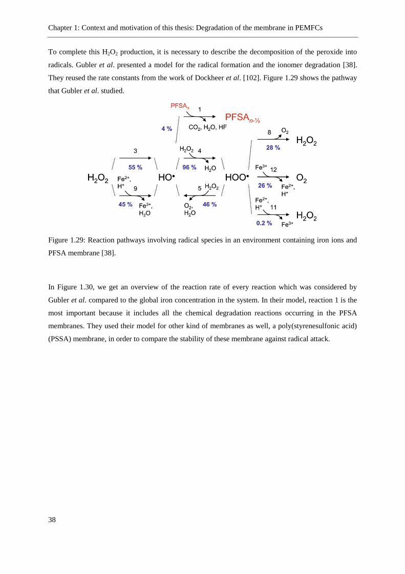
Chapter 1: Context and motivation of this thesis: Degradation of the membrane in PEMFCs
38
To complete this H2O2 production, it is necessary to describe the decomposition of the peroxide into
radicals. Gubler et al. presented a model for the radical formation and the ionomer degradation [38].
They reused the rate constants from the work of Dockheer et al. [102]. Figure 1.29 shows the pathway
that Gubler et al. studied.
Figure 1.29: Reaction pathways involving radical species in an environment containing iron ions and
PFSA membrane [38].
In Figure 1.30, we get an overview of the reaction rate of every reaction which was considered by
Gubler et al. compared to the global iron concentration in the system. In their model, reaction 1 is the
most important because it includes all the chemical degradation reactions occurring in the PFSA
membranes. They used their model for other kind of membranes as well, a poly(styrenesulfonic acid)
(PSSA) membrane, in order to compare the stability of these membrane against radical attack.

Chapter 1: Context and motivation of this thesis: Degradation of the membrane in PEMFCs
39
Figure 1.30: Reaction rates of reactions 1 and 3–13 (Figure 1.29, 13 is the reaction between ferric ions
and hydrogen peroxide) at a H2O2 concentration of 0.5 mM in the presence of PFSA ionomer with a
reactive end-group concentration [38].
To date, the most complete model describing the phenomena involved in the ionomer degradation has
been presented by Shah et al. [39]. Transport phenomena, thermal effects and charge conservation
were taken into account. They showed an interesting parametric study with discretization along the
membrane, as displayed in Figure 1.31. But in their model they ignore the side chain unzipping, which
means a constant conductivity of the membrane, and thus no effect of the degradation on the transport
phenomena and the cell performance can be simulated. If we compare this results with the values ex-
perimentally observed in Figure 1.28, we see a certain difference between the simulations of Shah and
Chen. This shows how important it is to validate a model (even partially) to give more reliability to the
simulation results which are difficult / impossible to get experimentally.

Chapter 1: Context and motivation of this thesis: Degradation of the membrane in PEMFCs
40
Figure 1.31: Evolutions of H2O2 concentrations for the base-case parameter values at the OCV: TAnode
= TCathode = 60 °C, PAnode = Pcathode = 300 kPa, no side-chain cleavage, and a constant Fe2+
concentration
of 5 ppm [39].
It has been experimentally observed that the potential decreases during operation. One contributor to
this decrease is the increasing of the membrane resistance. Fowler et al. used a so-called generalized
steady state electrochemical model (GSSEM) [103]. The ohmic losses are modeled by the use of
Ohm’s law. Figure 1.32, showed a comparison between a long-time experiment and simulation they
carried out. It presents a very good agreement but this kind of modeling has a drawback: It lays on the
use of empirical fitting of experiment. The simulations can only be carried out after getting the empiri-
cal equations required by the model. Such a model can unfortunately not be predictive, which means
that the model cannot be adapted to an another experiment without running it.
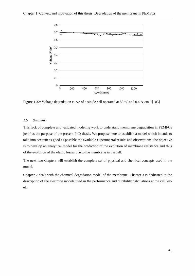
Chapter 1: Context and motivation of this thesis: Degradation of the membrane in PEMFCs
41
Figure 1.32: Voltage degradation curve of a single cell operated at 80 °C and 0.4 A·cm–2
[103]
1.5 Summary
This lack of complete and validated modeling work to understand membrane degradation in PEMFCs
justifies the purpose of the present PhD thesis. We propose here to establish a model which intends to
take into account as good as possible the available experimental results and observations: the objective
is to develop an analytical model for the prediction of the evolution of membrane resistance and thus
of the evolution of the ohmic losses due to the membrane in the cell.
The next two chapters will establish the complete set of physical and chemical concepts used in the
model.
Chapter 2 deals with the chemical degradation model of the membrane. Chapter 3 is dedicated to the
description of the electrode models used in the performance and durability calculations at the cell lev-
el.


Chapter 2: Modeling of the chemical degradation of the PFSA membrane
43
CHAPTER 2
Modeling of the chemical degradation of the PFSA
membrane
Une modélisation précise de membrane PFSA représente un réel challenge pour la science, tant
sa nanostructure reste en partie incomprise. Pour cette raison, nous nous contentons dans cette
approche de considérer la membrane comme un objet microscopique, en restant cependant co-
hérant avec les observations nanoscopiques qui ont été mentionnées dans le chapitre précédent.
Notre approche de la modélisation de la dégradation de la membrane se divise en deux parties,
la description des phénomènes de transport dans la membrane, et ensuite son extension et son
couplage aux phénomènes propres à la dégradation de la membrane.
La gestion de l’eau dans la membrane est un des aspects essentiels à maîtriser pour garantir une
durée de vie et des performances optimales de la pile. Lors du fonctionnement normal d’une
PAC, les protons sont produits à l’anode lors de la réaction d’oxydation de l’hydrogène, diffu-
sent le long de la membrane et sont ensuite consommés à la cathode lors de la réaction de réduc-
tion de l’oxygène. En solution aqueuse, les protons n’existant pas seuls, ceux-ci protonent les
molécules d’eau. Lorsqu’il est demandé à la cellule de produire du courant, celles-ci sont donc
transportées de l’anode à la cathode induisant un flux d’eau couplé à celui de protons. Ce flux
induit une accumulation partielle d’eau au niveau de la cathode, entraînant un déséquilibre dans
la répartition de l’eau dans le long de la membrane, déséquilibre d’autant plus grand que le cou-
rant demandé est élevé. La cellule va naturellement tendre vers un état d’équilibre, se traduisant
par un flux inverse d’eau de la cathode à l’anode. Ces deux phénomènes permettent de traiter
les aspects de la gestion de l’eau dans la membrane. L’équation transcrivant le flux d’eau en tout
point de la membrane est
y
tycD
F
itJ
),(··
OHFickOHOHOH
2
222
.
où le premier terme traduit le flux électroosmotique (mouvement des molécules d’eau avec les
protons) et le second terme le terme de diffusion retour, diffusion dite Fickienne. Afin de déter-
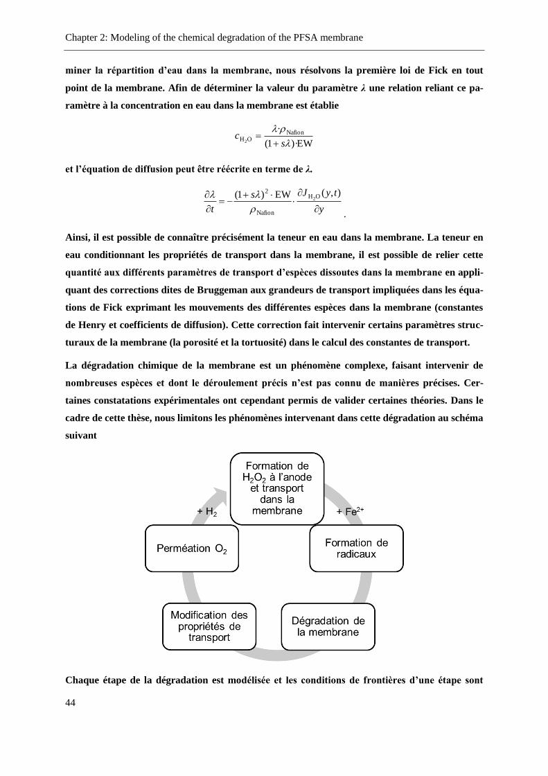
Chapter 2: Modeling of the chemical degradation of the PFSA membrane
44
miner la répartition d’eau dans la membrane, nous résolvons la première loi de Fick en tout
point de la membrane. Afin de déterminer la valeur du paramètre λ une relation reliant ce pa-
ramètre à la concentration en eau dans la membrane est établie
EW)·1(
· NafionOH2
sc
et l’équation de diffusion peut être réécrite en terme de λ.
y
tyJs
t
),(EW)1( OH
Nafion
22
.
Ainsi, il est possible de connaître précisément la teneur en eau dans la membrane. La teneur en
eau conditionnant les propriétés de transport dans la membrane, il est possible de relier cette
quantité aux différents paramètres de transport d’espèces dissoutes dans la membrane en appli-
quant des corrections dites de Bruggeman aux grandeurs de transport impliquées dans les équa-
tions de Fick exprimant les mouvements des différentes espèces dans la membrane (constantes
de Henry et coefficients de diffusion). Cette correction fait intervenir certains paramètres struc-
turaux de la membrane (la porosité et la tortuosité) dans le calcul des constantes de transport.
La dégradation chimique de la membrane est un phénomène complexe, faisant intervenir de
nombreuses espèces et dont le déroulement précis n’est pas connu de manières précises. Cer-
taines constatations expérimentales ont cependant permis de valider certaines théories. Dans le
cadre de cette thèse, nous limitons les phénomènes intervenant dans cette dégradation au schéma
suivant
Chaque étape de la dégradation est modélisée et les conditions de frontières d’une étape sont
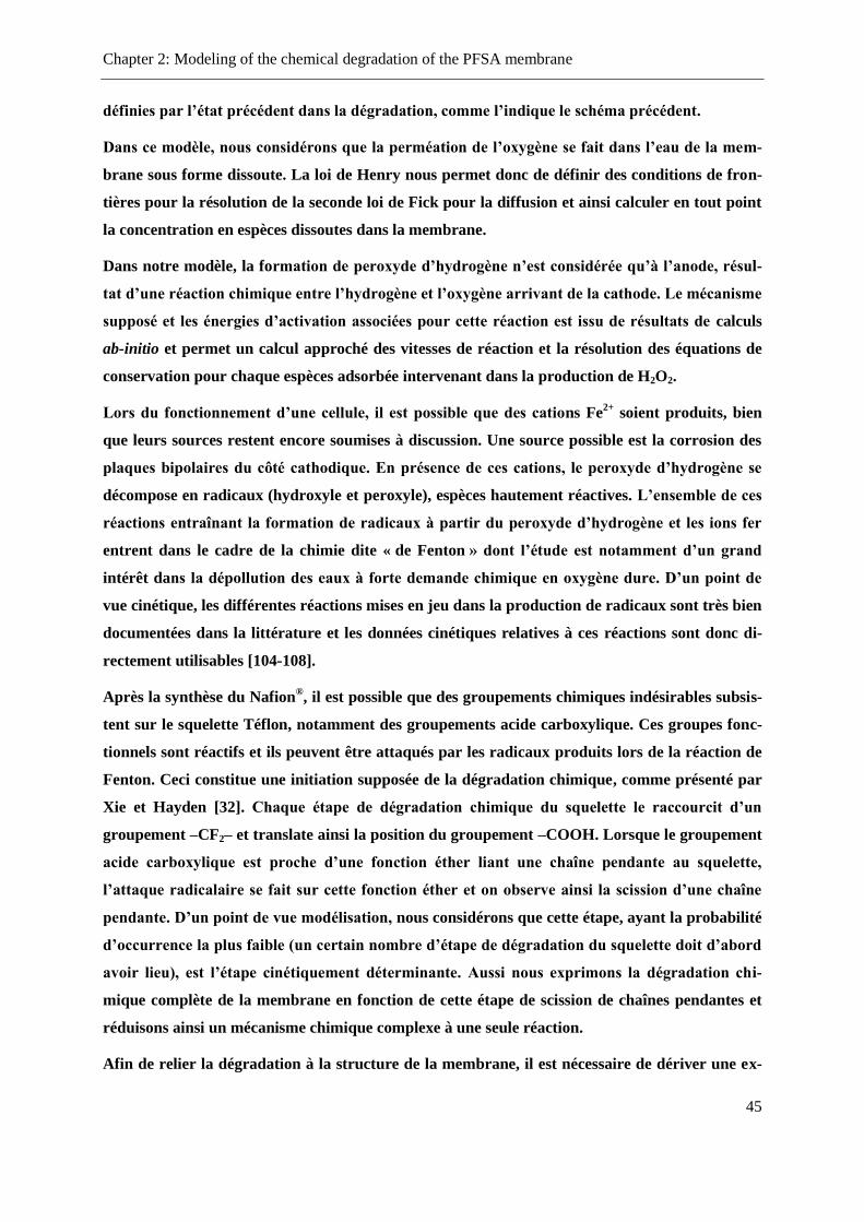
Chapter 2: Modeling of the chemical degradation of the PFSA membrane
45
définies par l’état précédent dans la dégradation, comme l’indique le schéma précédent.
Dans ce modèle, nous considérons que la perméation de l’oxygène se fait dans l’eau de la mem-
brane sous forme dissoute. La loi de Henry nous permet donc de définir des conditions de fron-
tières pour la résolution de la seconde loi de Fick pour la diffusion et ainsi calculer en tout point
la concentration en espèces dissoutes dans la membrane.
Dans notre modèle, la formation de peroxyde d’hydrogène n’est considérée qu’à l’anode, résul-
tat d’une réaction chimique entre l’hydrogène et l’oxygène arrivant de la cathode. Le mécanisme
supposé et les énergies d’activation associées pour cette réaction est issu de résultats de calculs
ab-initio et permet un calcul approché des vitesses de réaction et la résolution des équations de
conservation pour chaque espèces adsorbée intervenant dans la production de H2O2.
Lors du fonctionnement d’une cellule, il est possible que des cations Fe2+
soient produits, bien
que leurs sources restent encore soumises à discussion. Une source possible est la corrosion des
plaques bipolaires du côté cathodique. En présence de ces cations, le peroxyde d’hydrogène se
décompose en radicaux (hydroxyle et peroxyle), espèces hautement réactives. L’ensemble de ces
réactions entraînant la formation de radicaux à partir du peroxyde d’hydrogène et les ions fer
entrent dans le cadre de la chimie dite « de Fenton » dont l’étude est notamment d’un grand
intérêt dans la dépollution des eaux à forte demande chimique en oxygène dure. D’un point de
vue cinétique, les différentes réactions mises en jeu dans la production de radicaux sont très bien
documentées dans la littérature et les données cinétiques relatives à ces réactions sont donc di-
rectement utilisables [104-108].
Après la synthèse du Nafion®, il est possible que des groupements chimiques indésirables subsis-
tent sur le squelette Téflon, notamment des groupements acide carboxylique. Ces groupes fonc-
tionnels sont réactifs et ils peuvent être attaqués par les radicaux produits lors de la réaction de
Fenton. Ceci constitue une initiation supposée de la dégradation chimique, comme présenté par
Xie et Hayden [32]. Chaque étape de dégradation chimique du squelette le raccourcit d’un
groupement –CF2– et translate ainsi la position du groupement –COOH. Lorsque le groupement
acide carboxylique est proche d’une fonction éther liant une chaîne pendante au squelette,
l’attaque radicalaire se fait sur cette fonction éther et on observe ainsi la scission d’une chaîne
pendante. D’un point de vue modélisation, nous considérons que cette étape, ayant la probabilité
d’occurrence la plus faible (un certain nombre d’étape de dégradation du squelette doit d’abord
avoir lieu), est l’étape cinétiquement déterminante. Aussi nous exprimons la dégradation chi-
mique complète de la membrane en fonction de cette étape de scission de chaînes pendantes et
réduisons ainsi un mécanisme chimique complexe à une seule réaction.
Afin de relier la dégradation à la structure de la membrane, il est nécessaire de dériver une ex-

Chapter 2: Modeling of the chemical degradation of the PFSA membrane
46
pression de la porosité et la tortuosité en fonction de la structure chimique de la membrane. Ceci
est possible en faisant intervenir le concept de masse équivalente dans le calcul de la porosité et
d’utiliser une approche classique pour relier la tortuosité à la porosité (Equations 2.28 à 2.32).
La masse équivalente étant en relation directe avec la quantité de groupement acide sulfonique
dans la membrane, une évolution de cette quantité impactera directement sur la porosité.
A partir de cette évolution et compte tenu de la correction de Bruggeman utilisée, il est possible
de déterminer l’évolution de la résistance de la membrane au cours du fonctionnement de la pile
et de l’avancée de la dégradation. Il est ainsi possible de déterminer l’évolution des chutes oh-
miques dues à la résistance de la membrane et ainsi l’évolution de la tension de cellule.

Chapter 2: Modeling of the chemical degradation of the PFSA membrane
47
2 Modeling of the chemical degradation of the PFSA membrane
2.1 Introduction
As mentioned in Section 1.2.1, it is a real challenge to model a PFSA membrane in an exact way. To
get rid of the problem of an accurate description of membrane nanostructure, we consider the mem-
brane as a microscopic system, but with underlying concepts still consistent with observations from
the nano / microscale.
This chapter is divided into two main parts. First we will present the model used to describe the
transport processes in the membrane and then the concepts and equations behind the chemical degra-
dation model.
2.2 Modeling the transport processes in the membrane
2.2.1 Modeling of water management and transport
The proton conductivity of Nafion® is strongly dependent on the water content in the membrane. In-
deed a fully hydrated membrane will exhibit excellent proton conductivity, but when water content
decreases, the proton conductivity decreases. Thus water management in the membrane and in the
whole cell is one of the key aspects leading to efficient fuel cell operation. Two coupled mechanisms
are leading to dehydration of the membrane during fuel cell operation:
electro-osmotic drag, pulling water from anode to cathode,
a loss of water to fuel or air streams.
There is a considerable literature on the first mechanism, which focuses primarily on the water
transport mechanism within the membrane, assuming either a diffusive mechanism or a convective
one based upon phenomenological determined capillary pressure isotherms [109, 110]. In practical
applications the problem of a dry anode is solved by the use of a thin membrane (25 to 50 µm), which
facilitates the back diffusion of water and thus rehydrating the anode.
For a seek of simplicity we assume here:
a) isothermal conditions. The same temperature is set at both electrodes. No thermal exchanges
are taken into account.
b) GDL and electrodes are considered as hydrophobic, so that liquid water can be carried out of
the system.
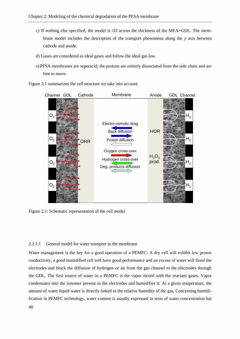
Chapter 2: Modeling of the chemical degradation of the PFSA membrane
48
c) If nothing else specified, the model is 1D across the thickness of the MEA+GDL. The mem-
brane model includes the description of the transport phenomena along the y axis between
cathode and anode.
d) Gases are considered as ideal gases and follow the ideal gas law.
e) PFSA membranes are superacid; the protons are entirely dissociated from the side chain and are
free to move.
Figure 2.1 summarizes the cell structure we take into account.
Figure 2.1: Schematic representation of the cell model
2.2.1.1 General model for water transport in the membrane
Water management is the key for a good operation of a PEMFC: A dry cell will exhibit low proton
conductivity, a good humidified cell will have good performance and an excess of water will flood the
electrodes and block the diffusion of hydrogen or air from the gas channel to the electrodes through
the GDL. The first source of water in a PEMFC is the vapor mixed with the reactant gases. Vapor
condensates into the ionomer present in the electrodes and humidifies it. At a given temperature, the
amount of water liquid water is directly linked to the relative humidity of the gas. Concerning humidi-
fication in PEMFC technology, water content is usually expressed in term of water concentration but
Cathode Anode
O2 H2
H2
H2
H2
O2
O2
O2
O2 H2
H2
H2
H2
O2
O2
O2
GDLGDLChannel ChannelMembrane
Electro-osmotic drag
Back diffusion
Oxygen cross-over
Hydrogen cross-over
O2 + 4H+ + 4e-
2 H2O
Proton diffusion
H2
2 H+ + 2 e-
H2 + O2
H2O2
Deg. products diffusion
(H2O2, radicals…)
Cathode AnodeMembrane0
y
ORR
HOR
H2O2
prod.
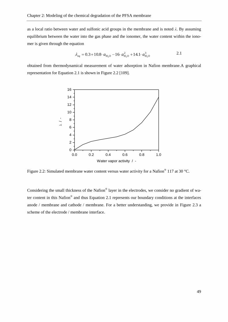
Chapter 2: Modeling of the chemical degradation of the PFSA membrane
49
as a local ratio between water and sulfonic acid groups in the membrane and is noted λ. By assuming
equilibrium between the water into the gas phase and the ionomer, the water content within the iono-
mer is given through the equation
3OH
2OHOH 222
1.14168.103.0 aaaeq 2.1
obtained from thermodynamical measurement of water adsorption in Nafion membrane.A graphical
representation for Equation 2.1 is shown in Figure 2.2 [109].
Figure 2.2: Simulated membrane water content versus water activity for a Nafion® 117 at 30 °C.
Considering the small thickness of the Nafion® layer in the electrodes, we consider no gradient of wa-
ter content in this Nafion® and thus Equation 2.1 represents our boundary conditions at the interfaces
anode / membrane and cathode / membrane. For a better understanding, we provide in Figure 2.3 a
scheme of the electrode / membrane interface.
0.0 0.2 0.4 0.6 0.8 1.0
0
2
4
6
8
10
12
14
16
/ -
Water vapor activity / -
Chapter 2: Modeling of the chemical degradation of the PFSA membrane
50
Figure 2.3: Schematic representation of the interface Electrode / Membrane (in gray color: ionomer).
The conservation equation of the water transport in a one dimensional coordinate within the membrane
is given by the second Fickian law
t
tyc
y
tyJ
),(),( OHOH 22 , 2.2
where OH2
J represents the local water flux and OH2c the local concentration of water. As λ represents
the water content in the membrane, it is possible to link it to the water concentration in the membrane.
Springer et al. derived such an expression, considering that the Nafion® swells with increasing water
uptake, which we assume as well [109].
EW)·1(
· NafionOH2
sc
2.3
is the relation established by Springer, where Nafion is the density of dry Nafion®, s is the swelling
coefficient and EW is the equivalent weight of the membrane. Equation 2.3 can be included into Equa-
tion 2.2. The simplification of the partial derivative leads to
y
tyJs
t
),(EW)1( OH
Nafion
22
.
2.4
We have now an explicit equation between the water content and the water flux in the membrane. The
next point is to get an expression for the water flux in the membrane (constitutive equation). Different
approaches are possible for that purpose. In our work, we use a semi-phenomenological one. When a

Chapter 2: Modeling of the chemical degradation of the PFSA membrane
51
current load is applied to a PEMFC, protons are required at the cathode side for the ORR. As protons
are always bound in complex cations in water (H3O+, H5O2
+, etc.), their motion from the anode to the
cathode induces a motion of water as well. A so-called drag coefficient (noted OH2t ) is introduced to
link this water flux to proton flux from the anode. If we assume no accumulation of protons within the
membrane, the Faraday’s law can be written
F
iJ H
, 2.5
where i is the current density and F the Faraday’s constant. From the last remark and Equation 2.5, we
get the expression of the electro-osmotic contribution in the model. As this flux is oriented from the
anode to the cathode, and our coordinate system is oriented from the cathode to the anode, we have to
correct with a negative sign and thus,
F
itJ ·OH
EOOH 22
, 2.6
which represents the electro-osmotic flux of water in the membrane. When no current is applied, no
protons are required and obviously this flux is equal to zero.
At the cathode side, water is produced by the ORR as shown on Reaction 1.2. From this production
and the electro-osmotic flux, the water balance in the membrane in not equilibrated anymore. This
means that a water gradient appears along the membrane. The anode becomes dryer and the cathode
trends to be flooded. This gradient causes a back flux of water from the cathode to the anode, in order
to equilibrate the water balance in the membrane [111]. This can be mathematically expressed by the
first Fickian law for the diffusion as
y
tycDJ
),(·
OHFickOH
BDOH
2
22,
2.7
where OH2
D is the diffusion coefficient of water in Nafion®.
Adding Equations 2.6 and 2.7, we get the expression of the net water flux within the membrane, as
y
tycD
F
itJ
),(··
OHFickOHOHOH
2
222.
2.8
Combining Equation 2.8 in Equation 2.4, we can simulate water content profile along the membrane.
To get a precise profile of the water content, it is however necessary to define precisely boundary con-
ditions for the system. These boundaty conditions will be slightly different depending on the simula-
tion environment which is used (see Section 3). Indeed, as MEMEPhys® includes an adapted version
of the membrane model of DENIS, the model must return water flow at interfaces membrane / elec-

Chapter 2: Modeling of the chemical degradation of the PFSA membrane
52
trodes as boundary for Equation 2.4. DENIS computes a water flux from the equivalent water content
calculated from Equation 2.1 and the value of the water content in the membrane close to the interface.
At the anode / membrane interface, the inlet flow is driven by the difference in water content between
the membrane at y = Lmembrane and the anode (where the water content is supposed to be equal to λeq).
There is here no difference between MEMEPhys® and DENIS, as no water is produced in the anode.
The same assumptions are made at the cathode / membrane interface (at y = 0). Moreover, water is
produced in the cathode catalyst layer and this has to be then linked with the cathode model. In DEN-
IS, the flux of produced water can be expressed through the Faraday’s law, giving
F
iJ
·2
prod
OH2 .
2.9
In MEMEPhys®, water is produced during the ORR by Reaction 3.14 (see Section 3.2.4.2). The rate of
the reaction determines the flux of water production by the ORR.
As in a real fuel cell not all of the produced water at the cathode is released in the membrane but can
leave the cell through the GDL and gas channel, we assume that the net water inlet due to the water
production is equal to
prod
OHmembeff prod,
OH 22·JJ , 2.10
where αmemb is an arbitrary coefficient between 0 and 1, and which indicates the fraction of water pro-
duced during the ORR, which remains in the membrane.
We can now define the boundary conditions at the interfaces anode catalyst layer / membrane and
membrane / cathode catalyst layer concerning the water flux. At the anode side, neglecting the evacua-
tion of water through the GDL / gas channel pathway, the only water movement that has to be consid-
ered is the water dissolution for the gas phase into the ionomer contained into the anode. The corre-
sponding water content is calculated through Equation 2.1. Assuming a uniformity of the water con-
tent in the anode catalyst layer, the water flux at the anode / membrane interface is driven by the gra-
dient in the water content between the anode and the membrane at y = Lmembrane. The boundary condi-
tion is then
membrane
2
anodeeqmemb
membrane / anodeOH ·
LyJ
. 2.11
At the cathode side, as previously said, water is produced. The flux of produced water can be quanti-
fied as shown on Equation 2.10. Considering the water flux between the gas channel and the ionomer
in the cathode, we get a second boundary condition for the water flux,
prod
OHmemb0cathode
eqmembmembrane / cathode
OH22
·· JJ y 2.12
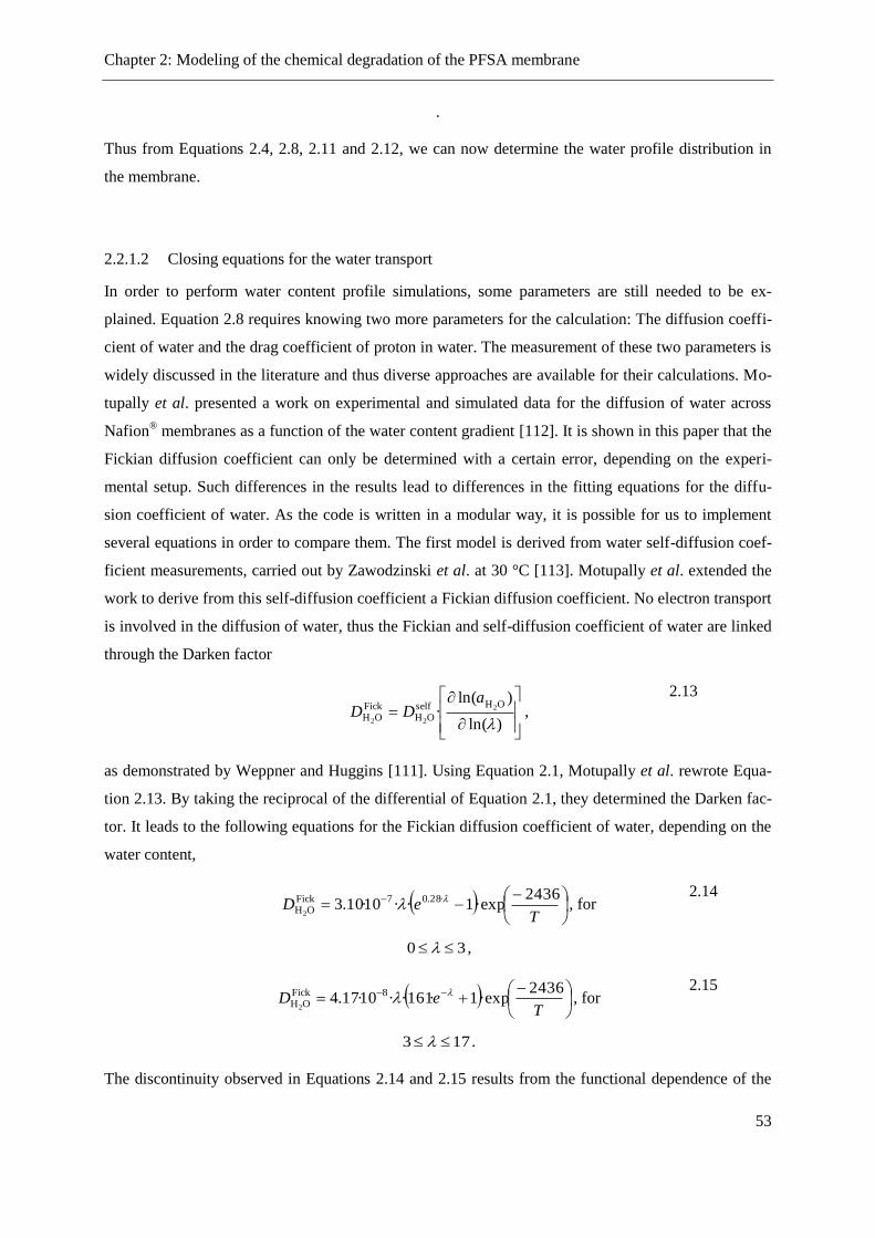
Chapter 2: Modeling of the chemical degradation of the PFSA membrane
53
.
Thus from Equations 2.4, 2.8, 2.11 and 2.12, we can now determine the water profile distribution in
the membrane.
2.2.1.2 Closing equations for the water transport
In order to perform water content profile simulations, some parameters are still needed to be ex-
plained. Equation 2.8 requires knowing two more parameters for the calculation: The diffusion coeffi-
cient of water and the drag coefficient of proton in water. The measurement of these two parameters is
widely discussed in the literature and thus diverse approaches are available for their calculations. Mo-
tupally et al. presented a work on experimental and simulated data for the diffusion of water across
Nafion® membranes as a function of the water content gradient [112]. It is shown in this paper that the
Fickian diffusion coefficient can only be determined with a certain error, depending on the experi-
mental setup. Such differences in the results lead to differences in the fitting equations for the diffu-
sion coefficient of water. As the code is written in a modular way, it is possible for us to implement
several equations in order to compare them. The first model is derived from water self-diffusion coef-
ficient measurements, carried out by Zawodzinski et al. at 30 °C [113]. Motupally et al. extended the
work to derive from this self-diffusion coefficient a Fickian diffusion coefficient. No electron transport
is involved in the diffusion of water, thus the Fickian and self-diffusion coefficient of water are linked
through the Darken factor
)ln(
)ln(·
OHselfOH
FickOH
2
22
aDD ,
2.13
as demonstrated by Weppner and Huggins [111]. Using Equation 2.1, Motupally et al. rewrote Equa-
tion 2.13. By taking the reciprocal of the differential of Equation 2.1, they determined the Darken fac-
tor. It leads to the following equations for the Fickian diffusion coefficient of water, depending on the
water content,
TeD
2436·exp1··10·10.3 ·28.07Fick
OH2
, for
30 ,
2.14
TeD
2436·exp1·161··10·17.4 8Fick
OH2
, for
173 .
2.15
The discontinuity observed in Equations 2.14 and 2.15 results from the functional dependence of the
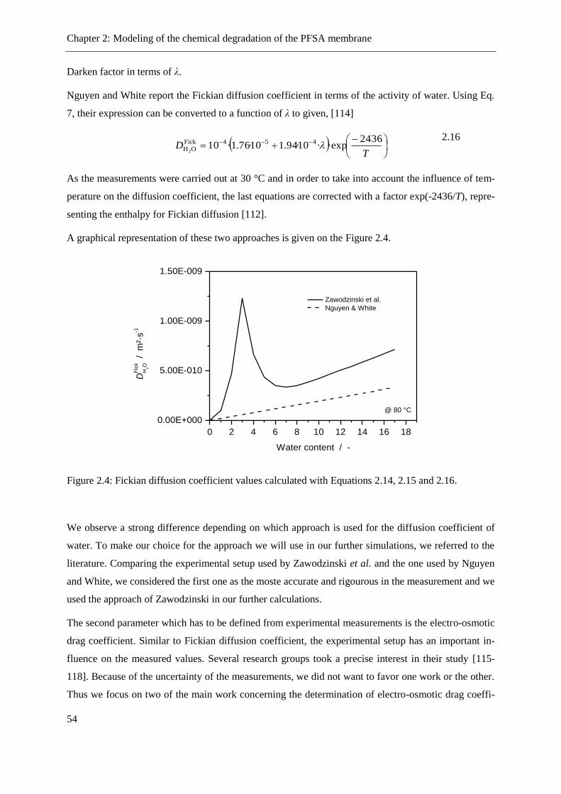
Chapter 2: Modeling of the chemical degradation of the PFSA membrane
54
Darken factor in terms of λ.
Nguyen and White report the Fickian diffusion coefficient in terms of the activity of water. Using Eq.
7, their expression can be converted to a function of λ to given, [114]
TD
2436·exp·10·94.110·76.1·10 454Fick
OH2
2.16
As the measurements were carried out at 30 °C and in order to take into account the influence of tem-
perature on the diffusion coefficient, the last equations are corrected with a factor exp(-2436/T), repre-
senting the enthalpy for Fickian diffusion [112].
A graphical representation of these two approaches is given on the Figure 2.4.
Figure 2.4: Fickian diffusion coefficient values calculated with Equations 2.14, 2.15 and 2.16.
We observe a strong difference depending on which approach is used for the diffusion coefficient of
water. To make our choice for the approach we will use in our further simulations, we referred to the
literature. Comparing the experimental setup used by Zawodzinski et al. and the one used by Nguyen
and White, we considered the first one as the moste accurate and rigourous in the measurement and we
used the approach of Zawodzinski in our further calculations.
The second parameter which has to be defined from experimental measurements is the electro-osmotic
drag coefficient. Similar to Fickian diffusion coefficient, the experimental setup has an important in-
fluence on the measured values. Several research groups took a precise interest in their study [115-
118]. Because of the uncertainty of the measurements, we did not want to favor one work or the other.
Thus we focus on two of the main work concerning the determination of electro-osmotic drag coeffi-
0 2 4 6 8 10 12 14 16 18
0.00E+000
5.00E-010
1.00E-009
1.50E-009
Zawodzinski et al.
Nguyen & White
DF
ick
H2O
/ m
²·s
-1
Water content / -
@ 80 °C

Chapter 2: Modeling of the chemical degradation of the PFSA membrane
55
cient in Nafion®.
The first one was published by Fuller and Newman [118]. Their set up was based on the generation of
a water activity gradient between two sides of a membrane and measuring the potential difference
which arises between two reversible H+/H2 electrodes on each side of the membrane.
Zawodzinski et al., inspired by the work of Fuller and Newman, improved the experimental set up of
the former [116]. They found out that the electro-osmotic drag coefficient is independent of the water
content and is equal to the unity as long as the membrane is in equilibrium with vapor (water under
gaseous form). However in presence of liquid water, the maximum water uptake is increased from 14
to 22, which impacts on the value of the drag coefficient (so-called Schroeder’s paradox)[119, 120].
The electro-osmotic drag coefficient is calculated by
1OH2t ,
for 140 ,
2.17
8
14.0-1.5· 1.0
OH2
t ,
for 2214 .
2.18
A later work for the determination of the electro-osmotic drag was reported by Ise, Kreuer and Meier
[115]. They applied electrophoretic NMR (ENMR) for the first time, in order to measure electro-
osmotic drag coefficients in polymer electrolyte membranes [121]. With this method, it is possible to
determine OH2t as a function of water content (without the requirement of different pretreatments of
the samples) and as a function of temperature. They measured the electro-osmotic drag coefficient at
several water content from 5 to 20. We interpolate linearly their results to get our last equation for the
calculation of the electro-osmotic drag,
44.1·10·6.4 2
OH2 t 2.19
As it can be seen in Figure 2.5, the value of the electro-osmotic drag strongly varies with water content
and analytical methodology. Thus it is interesting to further compare them and see how their impact
on the water management and cell performance is.
Both experimental setups provide drastically different results. To solve the problem of knowing which
results are the more representable of reality, we agree with a work of Meier and Eigenberger about
transport in Nafion® membrane [122]. They performed their own measurements of drag coefficient for
water content in membrane beyond 12. The results were in quite good agreement with the results of
Ise et al. and then they correlated their measurements with respect to the work of Zawodsinski when λ
trends to zero. Thus the correlation for drag coefficient which is used in our model is

Chapter 2: Modeling of the chemical degradation of the PFSA membrane
56
²·0026.0·028.01OH2
t . 2.20
This section showed how difficult it is, to establish a transport model for water in a PEMFC. Even if
the physics used to describe the motion of water molecule is only a sum of an EO drag and a Fickian
diffusion, the determination of the transport parameters needed to solve this equation is far more com-
plex and it is a real challenge for a modeler to decide, which measurement and approach could be the
closest from the modeled system.
Figure 2.5: Evolution of the electro-osmotic drag coefficient with water content
2.2.1.3 Motion of species through the membrane
As previously mentioned in Section 1.1.2, one role of the membrane is the separation of gases between
anode and cathode side, in order to prevent any short circuit. However, it has been experimentally
shown (as mentioned in Section 1.3.3) that Nafion® cannot prevent the oxygen or hydrogen to perme-
ate between the electrodes. It has been experimentally shown that the highest permeation of gases
between the electrodes occurs when the membrane is humidified (for example, the oxygen cross-over
is 10 time higher as for a dry membrane) [122]. Thus for a poorly hydrated membrane, the cross-over
is low. This value will increase with rising water content. This part will deal with the mathematical
formulation for the diffusion of non-charged hydrated species in the membrane.
As oxygen (resp. hydrogen) is present under gas form only at the cathode (resp. anode), a concentra-
tion gradient appears once the gases are dissolved in the ionomer phase. This concentration gradient
induces an oxygen flux from the cathode to the anode and a hydrogen flux from the anode to the cath-
ode. We first have to estimate the concentration of gases which effectively come into the ionomer at
0 2 4 6 8 10 12 14 16 18 20 22
0.0
0.5
1.0
1.5
2.0
Ise et al.
Linear fit of Ise et al.
Zawodzinski et al.
Meier & Eigenberger
Dra
g c
oe
ffic
ien
t /
-
Water content / -
Chapter 2: Modeling of the chemical degradation of the PFSA membrane
57
the GDL / electrode interfaces. As reactants are under a gaseous form in the channel but react in dis-
solved form in the electrodes, we have to express the dissolution process into the ionomer. For that
purpose we use the Henry’s law, (at a constant temperature, the amount of a given gas that dissolves in
a given type and volume of liquid is directly proportional to the partial pressure of that gas in equilib-
rium with that liquid)[40]. A mathematical formulation for this is
),elec/pore(··exp),elec/pore(
Henryact,
,0liq tP
R·T
EHtc i
i
ii
,
2.21
where H0,i is the reference Henry’s constant of species i, Henry
act,iE its activation energy, ),(liq tyci and
),( tyPi are the concentration and the partial pressure of species i in the ionomer phase at the interface
pore / ionomer. A part of these dissolved gases will react, depending on the power demanded to the
cell. The rest will be available to eventually diffuse along the membrane.
The motion of dissolved species in the membrane follows the conservation equation
²
),(²··exp
),( liqNafion Diffact,
,0
liq
y
tyc
R·T
ED
t
tyc ii
ii
,
2.22
where D0,i is the diffusion coefficient in Nafion® of solved species i and Nafion Diff
act,iE its activation ener-
gy. The boundary conditions of the Equation 2.22 are given by the Equation 2.21. However, as the
concentration of dissolved oxygen at the anode and dissolved hydrogen at the cathode are zero when
the cell starts, boundary conditions have to be time-dependent. It is not certain that the parasitic gas
will pass from the ionomer phase to the gas phase in the electrode. To solve this problem we assume
continuity in the ionomer at the membrane / electrode interface for parasitic gases and we set follow-
ing continuity equations at the interfaces membrane / electrode:
),anode(),( liq
Omembraneliq
O 22tyctLyc , 2.23
),cathode(),0( liq
H
liq
H 22tyctyc . 2.24
From Equation 2.21, linked to Equations 2.22, 2.23 and 2.24, we can now get the oxygen and hydro-
gen profile through the membrane.
This cross-over of oxygen from the cathode to the anode constitutes the first step in the chemical deg-
radation of the membrane.

Chapter 2: Modeling of the chemical degradation of the PFSA membrane
58
2.3 Modeling of chemical degradation of Nafion®
2.3.1 Chemical mechanism for Nafion® degradation
As shown in Section 1.2.2, the structure of Nafion® is very difficult to be defined and direct observa-
tions during operation of a PEMFC need a heavy and complicate experimental set up. This considera-
tion of the FC as a black box complicates the understanding of chemical degradation processes. There-
fore, experiments could give rise and quantify the presence of fluoride ions in the waste water of the
cell, as well as perfluorosulfonic acid and complex fluorated organic molecules [16, 31, 98, 100, 123-
125]. Assuming that in such experiment the eventual PTFE as additive in the GDL is stable, the only
possible fluoride source is the PFSA membrane. That would imply that the membrane has been de-
graded. After the analysis of several literature sources, we concluded to a series of steps explaining the
mechanism of the degradation, which is summed up in Figure 2.6.
Figure 2.6: Schematic representation of the causes-consequences of the chemical degradation
Hydrogen peroxide and anodic reactions – In the previous part, we described the permeation of oxy-
gen across the membrane from the cathode to the anode. It is to be noticed that at the same time, hy-
drogen can permeate from the anode to the cathode. As any further reaction of hydrogen at the cathode
is not taken into account, we do not consider it in our degradation scheme. The second part which has
to be regarded is the production of hydrogen peroxide from this oxygen. This reaction is linked to the
electrochemical reactions occurring at the anode. Thus the description of this phenomenon is ex-
plained in Section 3.2.4.1.
Influence on
transport
mechanism
Decrease of proton
conductivity
Decrease of cell
performance
Membrane
degradation
O2 crossover
CathodeAnode
H2O2
formation
H2O2
decomposition

Chapter 2: Modeling of the chemical degradation of the PFSA membrane
59
Radical formation – Hydrogen peroxide is used as a radical initiator [126]. In presence of so-called
Fenton’s ions (Fe or Cu), hydrogen peroxide is decomposed into hydroxyl or peroxide radicals. Its
action has already been discovered at the end of the 19th century by Henry Fenton and further studied
by Haber and Weiss [21, 127]. The decomposition of hydrogen peroxide into radicals belongs to a
broad field called Fenton chemistry. It includes a complete set of parallel reactions which have widely
been studied and whose kinetics coefficients have been measured (see also Appendix B). To simplify
our simulation and reduce the calculation time, we restrain all these reactions to five reactions which
we assumed as the major ones to describe the generation and consumption of radicals in the mem-
brane.
H2O2 decomposition – F1
(1st step)
H2O2 + Fe2+
+ H+ Fe
3+ + HO
· + H2O
Reaction 2.1
H2O2 decomposition – F2
(2nd
step) H2O2 + Fe
3+ Fe
2+ + HOO
· + H
+
Reaction 2.2
H2O2 decomposition – F3
(3rd
step) HOO
· + Fe
3+ Fe
2+ + O2 + H
+
Reaction 2.3
H2O2 decomposition – F4
(4th step)
H2O2 + HO· H2O + HOO
·
Reaction 2.4
H2O2 decomposition – F5
(5th step)
HO· + Fe
2+ + H
+ Fe
3+ + H2O
Reaction 2.5
From Reaction 2.1 and Reaction 2.2, we see the catalytic action of iron ions. In acidic media (like in
Nafion®), ferrous irons (Fe
2+) are oxidized by hydrogen peroxide into ferric irons (Fe
3+), hydroxyl
radicals and water. Fe3+
can be then reduced back to Fe2+
, a peroxide radical and a proton by hydrogen
peroxide (disproportionation of hydrogen peroxide – H2O2 is simultaneously reduced and oxidized).
The essential requirement for the decomposition of H2O2 is the presence of transition-metal ions in the
system. As this system is closed, these ions can only come from an internal source. Pozio et al.
showed that a PEMFC with stainless steel end-plates significantly degraded after 960 h of continuous
operation. By changing these end-plates with iron-free one, a little degradation was observed after
1200 h [89]. This point makes the modeling so difficult. The oxidation of the end-plate is a high ran-
dom phenomenon whose occurrence cannot be precisely known.
Membrane chemical degradation mechanisms –
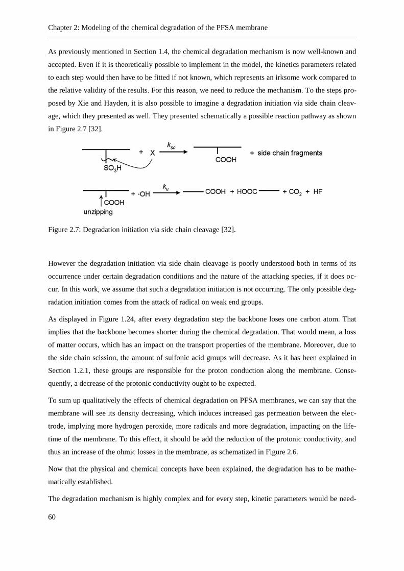
Chapter 2: Modeling of the chemical degradation of the PFSA membrane
60
As previously mentioned in Section 1.4, the chemical degradation mechanism is now well-known and
accepted. Even if it is theoretically possible to implement in the model, the kinetics parameters related
to each step would then have to be fitted if not known, which represents an irksome work compared to
the relative validity of the results. For this reason, we need to reduce the mechanism. To the steps pro-
posed by Xie and Hayden, it is also possible to imagine a degradation initiation via side chain cleav-
age, which they presented as well. They presented schematically a possible reaction pathway as shown
in Figure 2.7 [32].
Figure 2.7: Degradation initiation via side chain cleavage [32].
However the degradation initiation via side chain cleavage is poorly understood both in terms of its
occurrence under certain degradation conditions and the nature of the attacking species, if it does oc-
cur. In this work, we assume that such a degradation initiation is not occurring. The only possible deg-
radation initiation comes from the attack of radical on weak end groups.
As displayed in Figure 1.24, after every degradation step the backbone loses one carbon atom. That
implies that the backbone becomes shorter during the chemical degradation. That would mean, a loss
of matter occurs, which has an impact on the transport properties of the membrane. Moreover, due to
the side chain scission, the amount of sulfonic acid groups will decrease. As it has been explained in
Section 1.2.1, these groups are responsible for the proton conduction along the membrane. Conse-
quently, a decrease of the protonic conductivity ought to be expected.
To sum up qualitatively the effects of chemical degradation on PFSA membranes, we can say that the
membrane will see its density decreasing, which induces increased gas permeation between the elec-
trode, implying more hydrogen peroxide, more radicals and more degradation, impacting on the life-
time of the membrane. To this effect, it should be add the reduction of the protonic conductivity, and
thus an increase of the ohmic losses in the membrane, as schematized in Figure 2.6.
Now that the physical and chemical concepts have been explained, the degradation has to be mathe-
matically established.
The degradation mechanism is highly complex and for every step, kinetic parameters would be need-

Chapter 2: Modeling of the chemical degradation of the PFSA membrane
61
ed. Such an approach would be very time consuming and approximate, as we would have fitted every
kinetic parameters we used. For this reason, we have to find a way to simplify the system. As men-
tioned in the previous chapter, the degradation is initiated by a radical attack on weak end group, and
during the degradation, it occurs that a side chain are cut from the backbone every time the backbone
degradation step is reached a certain time. Thus we assume in our model that regarding the whole
chemical degradation, the side chain unzipping is the rate-determining step. Thus we express the kinet-
ic of the back bone degradation as a linear function of the side chain degradation.
2.3.2 Mathematical formulation of the chemical degradation
The first step of the modeling of the chemical degradation is to determine the evolution and the spatial
distribution of the species involved during the degradation. For that we apply first the law of mass
action (Equation 2.25) for the expression of reaction rates,
ij
jiijitycktyv
reaction in involved species
membrane ,)),((,
,
2.25
where tyri , is the reaction rate of the reaction i at time t and at the coordinate y in the membrane, ki
the reaction rate constant of the reaction i, ),(membrane tyc j the concentration of the species j at time t and
at the coordinate y in the membrane, and ji , is the reaction order relate to species j in reaction i. The
reactions considered by the index i are the step of the Fenton chemistry (Reaction 2.1 to Reaction 2.5)
and the degradation step related to the side chain unzipping. The temporal evolution of the concentra-
tion in the membrane is then given by solving an equation system constituted by the mass balance
equation of each species (Equation 2.26)
ji
ijijj
tyvSt
tyc
species involvingreaction
,
membrane
,·),(
,
2.26
where jS
is the production term of species j used for example in the case of hydrogen peroxide,
whose concentration is given by the electrochemistry at the anode and ferrous ions, whose production
is arbitrary set by the user of the model (see Section 4.2.3.4).
From Equations 2.25 and 2.26, it is possible to determine the evolution of species concentration along
the membrane. This will be the starting point for the rest of the modeling. From the evolution of the
concentration, we will be able to define the evolution of structural parameters of the membrane (poros-
Chapter 2: Modeling of the chemical degradation of the PFSA membrane
62
ity and tortuosity), which will impact on the performance of the cell.
As mentioned in Section 1.3.5, fluoride ion is a degradation product which is easy to measure and
follow over time with simple analytical methods (for example ionic chromatography or with a fluoride
sensitive sensor). As we consider in our approach only the kinetic of the side chain scission, we need a
way to however estimate the global amount of released fluoride. If we assume that the back bone is
degraded on a linear way, it will occur that the carboxylic acid group of the backbone is located on a
α-position of a side chain. That would imply that the steric factor becomes negligible and it is possible
for the radical to attack the ether function of the PFSA membrane. Considering this, we assume that
the rate determining step of the membrane degradation is the side chain scission, and thus, the kinetic
of release of fluoride ions is driven by the velocity of side chain scission. When the scission of a side
chain occur, that mean that roughly 15 –CF2– and one –CF– groups of the back bone have been cut,
thus 31 fluoride atoms are released into the membrane through the backbone. As a side chain contains
10 fluoride atoms, we come to an estimated ratio side chain to fluoride of 1 to 41 in Nafion®. In term
of mass balance equation, it comes
t
tyc
t
tyc
),(·41
),( membraneFluoride
membranechain side
.
2.27
Evolution of structural parameters – In the following parts and in the rest of this work, we will speak
about the porosity ε of the membrane even if this concept does not really suit to a PFSA membrane.
Indeed no porous structure can be identified. This porosity refers rather to the volume fraction of wa-
ter. We can then write
r
,
2.28
where OHNAFION 2
VVr is the ration of partial molar volume of membrane to that of water.
The partial molar volume of membrane can be expressed as a function of the equivalent weight of the
membrane EW and the density of the dry polymer ρdry as dryNAFION EWV . As the equivalent weight
can be expressed as
chain side
3
dry ··1 csEW , 2.29
where s is the swelling coefficient of the membrane (factor showing the variation of the membrane
volume by water uptake), and the side chain concentration depends on the position in the membrane
and time (when degradation occurs), we can simplify the expression for the partial molar volume of
the membrane in
Chapter 2: Modeling of the chemical degradation of the PFSA membrane
63
1
chain side
3
NAFION ),(··1),(
tycstyV . 2.30
Tortuosity and porosity are two parameters whose evolutions are dependent on each other: when the
porosity of the cell decreases, the tortuosity will increase. Several expressions for tortuosity have been
proposed for porous media and membranes based on the statistical analysis of diffusion coefficients,
free volume theory and power series expansion etc. [128-130]. These models provide similar values of
tortuosity factors for Nafion® for the sorption range of interest. Here, we adopt Prager’s model which
has been previously used for Nafion® by Koter and by Choi et al [130, 131]
·ln)1·(
)·(ln·5.0·ln·2)1·(22
2
.
2.31
We see in Figure 2.8 that with Prager’s model, the tortuosity increases to values which are unrealistic
when the porosity trend to zero. To check the validity of this approach, we compared the results we
obtained with a more common equation used to describe the relative evolution of porosity and tortuos-
ity,
1 .
2.32
From a porosity of 0.2, results of Prager’s model are in a range which is more consistent with the val-
ue of a tortuosity. From a porosity of about 0.4, we see that both approaches have comparable results.
After each simulation, we controlled these two parameters. The porosity never decreases under 0.2;
therefore, we kept Equation 2.31 in our simulations.
From Equations 2.28, 2.30 and 2.31, it is now possible to determine the structural evolution of the
membrane. It ought now to link these evolutions with their impact on the transport and the perfor-
mance of the cell. A comparison of the relative evolution is plotted in Figure 2.8. As we can see, a
high porosity in the membrane will induce a low tortuosity, which means degraded transport proper-
ties.
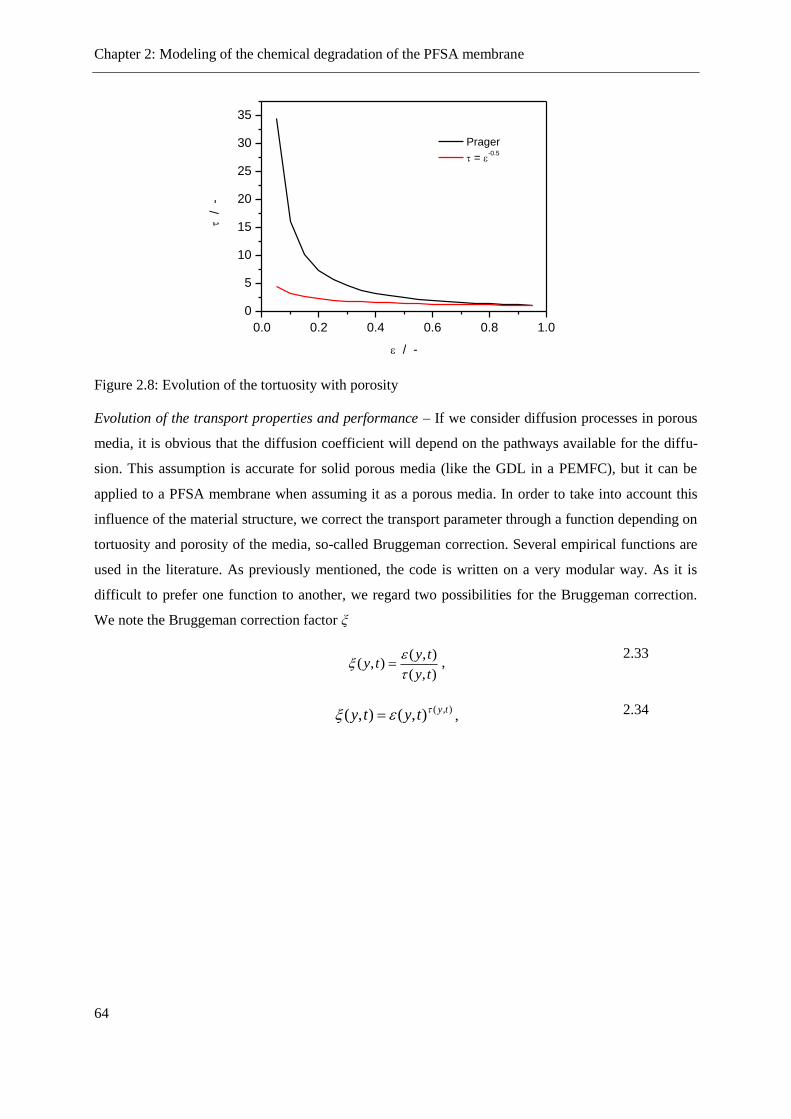
Chapter 2: Modeling of the chemical degradation of the PFSA membrane
64
Figure 2.8: Evolution of the tortuosity with porosity
Evolution of the transport properties and performance – If we consider diffusion processes in porous
media, it is obvious that the diffusion coefficient will depend on the pathways available for the diffu-
sion. This assumption is accurate for solid porous media (like the GDL in a PEMFC), but it can be
applied to a PFSA membrane when assuming it as a porous media. In order to take into account this
influence of the material structure, we correct the transport parameter through a function depending on
tortuosity and porosity of the media, so-called Bruggeman correction. Several empirical functions are
used in the literature. As previously mentioned, the code is written on a very modular way. As it is
difficult to prefer one function to another, we regard two possibilities for the Bruggeman correction.
We note the Bruggeman correction factor ξ
),(
),(),(
ty
tyty
,
2.33
),(),(),( tytyty , 2.34
0.0 0.2 0.4 0.6 0.8 1.0
0
5
10
15
20
25
30
35
Prager
= -0.5
/
-
/ -
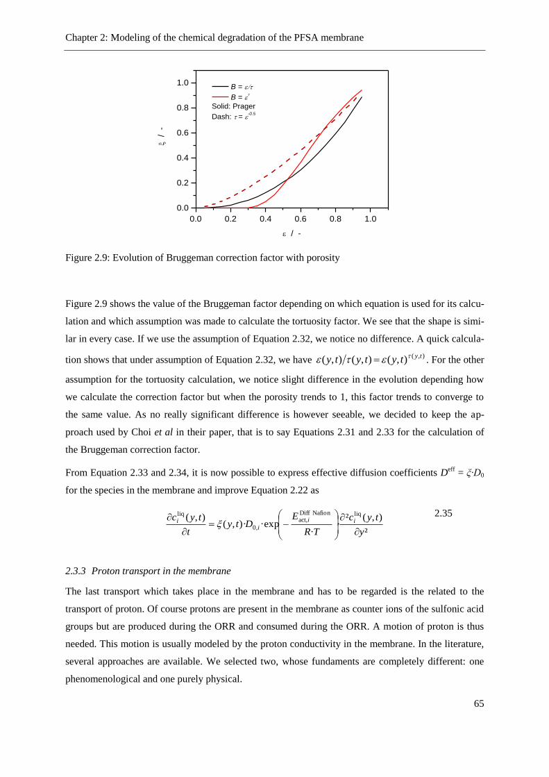
Chapter 2: Modeling of the chemical degradation of the PFSA membrane
65
Figure 2.9: Evolution of Bruggeman correction factor with porosity
Figure 2.9 shows the value of the Bruggeman factor depending on which equation is used for its calcu-
lation and which assumption was made to calculate the tortuosity factor. We see that the shape is simi-
lar in every case. If we use the assumption of Equation 2.32, we notice no difference. A quick calcula-
tion shows that under assumption of Equation 2.32, we have ),(),(),(),( tytytyty . For the other
assumption for the tortuosity calculation, we notice slight difference in the evolution depending how
we calculate the correction factor but when the porosity trends to 1, this factor trends to converge to
the same value. As no really significant difference is however seeable, we decided to keep the ap-
proach used by Choi et al in their paper, that is to say Equations 2.31 and 2.33 for the calculation of
the Bruggeman correction factor.
From Equation 2.33 and 2.34, it is now possible to express effective diffusion coefficients Deff
= ξ·D0
for the species in the membrane and improve Equation 2.22 as
²
),(²··exp)·,(
),( liqNafion Diffact,
,0
liq
y
tyc
R·T
EDty
t
tyc ii
ii
2.35
2.3.3 Proton transport in the membrane
The last transport which takes place in the membrane and has to be regarded is the related to the
transport of proton. Of course protons are present in the membrane as counter ions of the sulfonic acid
groups but are produced during the ORR and consumed during the ORR. A motion of proton is thus
needed. This motion is usually modeled by the proton conductivity in the membrane. In the literature,
several approaches are available. We selected two, whose fundaments are completely different: one
phenomenological and one purely physical.
0.0 0.2 0.4 0.6 0.8 1.0
0.0
0.2
0.4
0.6
0.8
1.0 B =
B =
Solid: Prager
Dash: = -0.5
/ -
/ -
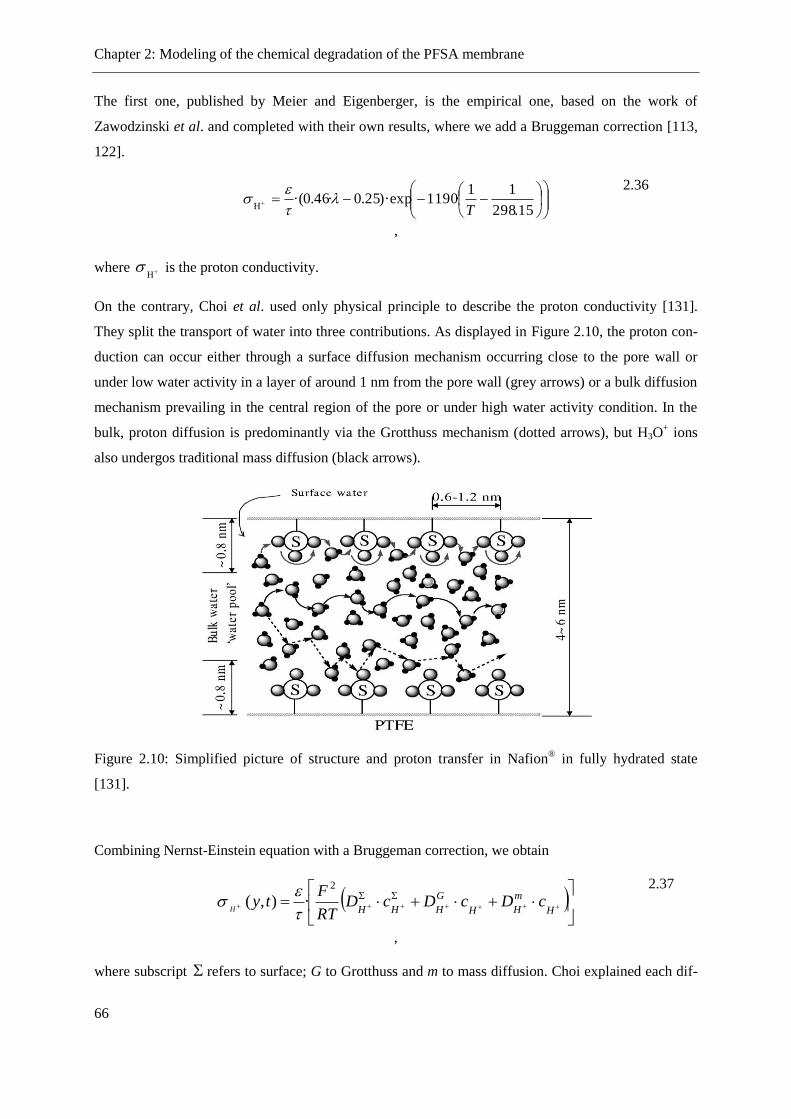
Chapter 2: Modeling of the chemical degradation of the PFSA membrane
66
The first one, published by Meier and Eigenberger, is the empirical one, based on the work of
Zawodzinski et al. and completed with their own results, where we add a Bruggeman correction [113,
122].
15.298
11·1190)·exp25.0·46.0·(
H T
,
2.36
where H is the proton conductivity.
On the contrary, Choi et al. used only physical principle to describe the proton conductivity [131].
They split the transport of water into three contributions. As displayed in Figure 2.10, the proton con-
duction can occur either through a surface diffusion mechanism occurring close to the pore wall or
under low water activity in a layer of around 1 nm from the pore wall (grey arrows) or a bulk diffusion
mechanism prevailing in the central region of the pore or under high water activity condition. In the
bulk, proton diffusion is predominantly via the Grotthuss mechanism (dotted arrows), but H3O+ ions
also undergos traditional mass diffusion (black arrows).
Figure 2.10: Simplified picture of structure and proton transfer in Nafion® in fully hydrated state
[131].
Combining Nernst-Einstein equation with a Bruggeman correction, we obtain
H
m
HH
G
HHHcDcDcD
RT
Fty
H
2
·),(
,
2.37
where subscript refers to surface; G to Grotthuss and m to mass diffusion. Choi explained each dif-

Chapter 2: Modeling of the chemical degradation of the PFSA membrane
67
fusion coefficient using Einstein-Smoluchowski equation and obtained
)RR·(RR·
·····4
²·exp
4·
·
ififBr0
B
H l
l
Tk
el
h
TkD
,
2.38
2θ
tan
2θ
tan
ln·R···η··192
)··(·
F
I
230r
2
HW2
H
ezlD
GG ,
2.39
i
B
H η·R·6·
·
TkDW
, 2.40
the parameters related to each equation and their value are given in Symbols parts [131].
For comprehension purpose, how all those parameters can be used in the calculation of diffusion coef-
ficients of protons, some figures can be used to illustrate the theory.
Figure 2.11: A schematic representation of the first proton hopping at the surface of Nafion® (a) before
and (b) after the first jump [131].
Figure 2.12: The hydrodynamic model of Grotthuss diffusion mechanism of protons in the pore bulk
[131].
Chapter 2: Modeling of the chemical degradation of the PFSA membrane
68
Figure 2.11 shows schematically the proton transfer in Nafion® from the sulfonate group of a side
chain to a close located water molecule (state (a) to state (b)). Then the proton will hop from a “free”
hydronium ion to a water molecule bond to a side chain, making the surface diffusion possible.
Figure 2.12 present the geometrical requirement for a proton to be able, in the bulk water area of a
channel, to hop from a hydronium ion to a water molecule. As the water is omnipresent in the mem-
brane at a sufficient state of humidification and considering the entropy of the system high enough, the
probability that one water molecule is ideally located compared to a hydronium ion is high and make
the contribution of this diffusion as major in good humidified membrane. The en masse expression is
the expression of the Stockes-Einstein equation considering hydronium ion as a diffusing entity a con-
tinuum of water.
Now we have all relationship for the calculation of proton conductivity in Equation 2.37 except the
one for the concentration of proton in at the surface of the pore and in the bulk water.
Because of the electroneutrality principle applied to the membrane, the concentration of hydronium
ions is equal to the one of sulfonic acid groups. But its distribution has to be cleared. Choi used an
approach in which the dissociated acid sites with up to two water molecules are assumed to remain
close to the surface and are designated as surface water, while those with more than two water mole-
cules are assumed to move away from the surface into the pore bulk, based on the hypothesis that sul-
fonic acid groups are sufficiently strong acids so that ion pairs OHSO 33 or
253 OHSO are formed
[131]. It comes out the following expressions for the proton distribution, depending on water content
and relative humidity (activity of water vapor)
)1·(··KK)·K1)·(1(
)·K1)·(1·(·K·
V·
11v2
211
21
OHH
2
aaaa
aaac
,
2.41
)1·(··KK)·K1)·(1(
)1·(··KK·
V·
11v2
211
2v321
OHH
2
aaaa
aac
,
2.42
where K1 and K2 are the equilibrium constants for proton dissociation in the membrane, a the activity
of water, OH2V the molar volume of water and v the amount of water molecules surrounding one
hydronium. From Equations 2.38 to 2.42, it is now possible to calculate the proton conductivity
through Equation 2.37.
The use of this local conductivity is then used by DENIS in the calculation of the ionic potential across
the membrane through the solving of Laplace equation (see Section 3.3.2).
However, for MEMEPhys®, a local value of the proton conductivity in the membrane is not used. The
transport parameter which is effectively used in the potential calculation is the membrane resistance.

Chapter 2: Modeling of the chemical degradation of the PFSA membrane
69
So it is needed to compute equivalent proton conductivity for the whole membrane to be able to com-
pute the global resistance of the membrane. In a general 1D case, we have to consider a series circuit
with conductance. The resulting equivalent conductance will be
membrane
0membrane
1
eq),(
·1
)(Ly
y ty
dy
Lt
H
. 2.43
From the equivalent proton conductivity, we calculate the membrane resistance as
)(·)(
eqelectrode
membrane
tS
EtR
.
2.44
It is now possible to evaluate the evolution of the membrane ohmic losses ηohm(t)=R(t)·I and thus eval-
uate the impact of the chemical degradation of the membrane on the cell performance.
2.4 Summary
We presented in this chapter first a transport model for water and dissolved species in the membrane
of a PEMFC. Water management is one of the key of the operating of the cell, as water is involved
among other in proton conduction and species diffusion. This model is based on classical work pub-
lished in the literature, extended with a permeation model for dissolved gases in the membrane. The
approach allows then a feedback between membrane degradation and membrane micro-structure,
through the calculation of the evolution of the porosity and the tortuosity.


Chapter 3: Coupling of the membrane model with the cell models
71
CHAPTER 3
Coupling of the membrane model with the cell mod-
els
La section précédente présentait le modèle de membrane incluant la dégradation chimique. Il
convient maintenant de coupler ce modèle avec des modèles d’anode et de cathode afin de simu-
ler le fonctionnement complet d’une PAC. Le modèle de membrane a été développé conjointe-
ment entre le centre aérospatial allemand (DLR) à Stuttgart et le Commissariat à l’Energie
Atomique et Energies Alternatives (CEA) à Grenoble. Les groupes de travail au sein desquels le
travail a été effectué, bien qu’utilisant à terme le même modèle de membrane, ont développé
séparément leurs propres modèles d’électrodes.
Pour cette raison, notre modèle de membrane a été codé de sorte à être utilisable dans les deux
environnements de simulation, le modèle CEA étant développé sous MATLAB/Simulink, le mo-
dèle DLR en langage C. Cet aspect a été traité grâce à la souplesse de Simulink, qui peut intégrer
dans ces modules des fonctions codées en C. Ainsi un modèle de membrane codé en langage C
permet à la fois d’être intégré directement dans les environnements développés au CEA et au
DLR.
Au CEA, le modèle d’électrodes développé, appelé MEMEPhys® (Modèle Electrochimique Mul-
ti-Echelle Physique) se base sur une approche multiphysique et multiéchelle des phénomènes se
déroulant dans les électrodes d’une PAC. Ce modèle se base sur une description précise de la
double couche électrochimique se formant à la surface du catalyseur. Cette approche permet un
calcul de la tension de cellule à partir du courant demandé à la cellule. Une description complète
du modèle ne fait pas l’objet de ce résumé, mais celui-ci est disponible dans de nombreuses
sources dans la littérature [132-134]. Le couplage du modèle de membrane au modèle
d’électrodes se fait via la calcul de la résistance de la membrane.
Le modèle développé au DLR, nommé DENIS (Detailed Electrochimistry and Numerical Impe-
dance Simulation), fut à l’origine conçu pour la simulation du fonctionnement de PAC de type
SOFC. Ce modèle a été maintes fois éprouvé et validé dans la littérature [135, 136]. Le principe a
été transposé au PEMFC et un modèle de performance a été établi et validé [137]. Cet environ-
Chapter 3: Coupling of the membrane model with the cell models
72
nement a connu ces dernières années d’importantes modifications, notamment au niveau de
l’approche utilisée dans les calculs électrochimiques. Le code utilise l’environnement CANTERA
pour la définition des phases dans les électrodes et le calcul des potentiels et compositions des
différentes phases. Une description complète de l’approche physique utilisée dans CANTERA
est détaillée dans sa documentation [138].
Ces deux modèles ont chacun leurs points forts et faiblesse dans l’approche. Afin d’effectuer une
comparaison des deux approches physiques mises en jeu dans les modèles, le modèle de mem-
brane est intégré dans chaque environnement. Cependant sur la durée de cette thèse, la mem-
brane n’a pu être couplée que dans l’environnement MEMEPhys®. Un couplage complet avec
DENIS fait l’objet de projets en cours.

Chapter 3: Coupling of the membrane model with the cell models
73
3 Coupling of the membrane model with electrode and cell models
3.1 Why cell models?
As said at the beginning of Chapter 0, the membrane model aims to be integrated into two different
simulation packages. Both have their own specificities, in particular on the level of detail of the phys-
ics used to describe the electrochemical and transport phenomena in the PEMFC components.
3.1.1 DENIS
DENIS (detailed electrochemistry and numerical impedance simulation) is a C code that is developed
since 2003 within the group of Wolfgang Bessler successively at the Interdisciplinary Center for Sci-
entific Calculation (IWR) of the University of Heidelberg and at the Institute for Technical Thermo-
dynamics at the German Aerospace Center in Stuttgart. Simulations are carried out, based on conven-
iently editable text input files for all modeling and simulation parameters. The software allows the
automated generation of current/voltage curves and electrochemical impedance spectra. Finite-volume
discretization techniques are used to convert the partial differential equations (PDE) occurring in the
transport models to a differential algebraic equation (DAE) system. Discretization is needed for the
two dimensions (x: along the gas channel, y: through MEA). The 1D+1D mesh can be set arbitrarily,
i.e. variable numbers and sizes of discretization compartments, so that a dense number of grid points
can be used for regions of strong gradients. Based on text input files of chemical reaction mechanisms
(pre-exponential factors, activation energies, thermodynamic properties), chemical source terms are
calculated using algorithms from the CANTERA software package. CANTERA is also used to calcu-
late gas-phase transport properties [139]. For numerical integration of the DAE system, the fully im-
plicit solver LIMEX is implemented [140, 141] . The implementation is carried out in a flexible and
modular way. Different sub-models can be coupled in user-defined ways. The software package can be
used for detailed or global chemistry, for 0D, 1D, quasi-2D or quasi-3D simulations where arbitrary
transport models can be coupled, for dual-chamber and single-chamber setups, for full-cell and refer-
ence electrode setups.
3.1.2 MEMEPhys®
The group headed by Alejandro Franco develops since 2002 at CEA-LITEN a transient, multi-scale
and multiphysics single PEMFC model (called MEMEPhys® –French abbreviation for Multiscale elec-
trochemical-physical model) accounting for the coupling between self-consistent physical mechanistic
Chapter 3: Coupling of the membrane model with the cell models
74
descriptions of the physicochemical phenomena (e.g., reactants, water and charge transport and de-
tailed electrochemistry, materials aging mechanisms) taking place in the electrodes, the PEM, the
GDLs and the channels [5, 133, 134]. This model was designed to connect atomistic phenomena (ele-
mentary kinetic processes) with macroscopic electrochemical observables (e.g. polarization curves,
Electrochemical Impedance Spectra, cyclic voltammetry, cell potential decrease over time…) with
reasonable computational effort by using ab initio and surface science databases [3-5, 133, 134]. Such
a model is a multi-scale one in the sense that it is made of a set of interconnected sub-models describ-
ing the phenomena occurring at different scales in the PEMFC. However, this description remains at
the continuum level in the sense that it is based on irreversible thermodynamics concepts particularly
adapted for the description of non-equilibrium physicochemical systems, as they are extensively used
in chemical engineering: use of conservation laws coupled to closure equations (e.g. flux expressions,
chemical rate models, thermodynamic models).
To the best of our knowledge, this model is the unique in published literature allowing describing the
feedback between the instantaneous performance and the intrinsic MEA aging processes: that means
that the model takes into account, at each simulated time step, both the effect of performance on aging
and the effect of aging on performance [3-5, 8]. The model is constituted by a hybridation between a
set of C modules and a Matlab/Simulink environment. It allows discretizing the cell into 1D (across
the cell thickness) + 1D (along the channels).
3.1.3 Membrane simulation code
DENIS and MEMEPhys® do not have anything in common concerning the implementation. As we
wanted to develop a generic module to limit the programming work and allow a direct comparison of
the physics used in electrodes with both their advantages and drawbacks, we needed a solution so that
the membrane model can be used by both simulation environments with minimum adaptation efforts.
Matlab proposes in its Simulink package the possibility to execute functions written in C through the
so-called S-functions. An S-function is a computer language description of a Simulink block written in
MATLAB®, C, C++, or FORTRAN. As DENIS was developed in C as well, the use of S-Function is
an elegant solution to use as a module in MEMEPhys®. The challenge is to provide to Matlab the tools
needed by the membrane module (called polymermembrane.c) to work correctly. In the membrane
module, arrays are defined and in DENIS, the allocation of array is done in an external module (called
memory.c). As polymermembrane.c is developed for the solving of DAE, mathematical functions are
required. These are contained in DENIS in a module called mathlib.c. For all other functions which are
used in polymermembrane.c but which refer to another module (for example to the module responsible
for thermal calculation etc.), the needed function are put into a specific module.

Chapter 3: Coupling of the membrane model with the cell models
75
DENIS works with specific input files, where all the parameters (diffusion coefficients, discretization
of the membrane, physical and chemical parameters for the cell etc.) are entered. As it is not possible
to use it directly with Simulink, we had to create a new module integrating all the parameters which
are used by polymermembrane.c.
Last polymermembrane.c needs and returns information from and to the Simulink model. These are
the inputs and outputs of the S-Function. A specific module ensures the communication between Sim-
ulink and the S-Function.
A schematically representation of the architecture of our S-Function is displayed in
Figure 3.1.
Figure 3.1: Structure of the S-Function implemented in Simulink to run our membrane module
3.2 Physics underlying the MEMEPhys® model
3.2.1 Presentation of the model
Since 2002, Franco and his successive collaborators have developed a dynamic numerical multiscale
model of a single PEMFC, based on non-equilibrium thermodynamics and electrodynamics, as pre-
sented in Figure 3.2 [3, 4, 85, 133, 134]. The model calculates, dynamically, the potential difference
between the two electrodes in response to a time dependent current demand. The major work concern-
ing the electrode models were published by Franco et al. since 2005 where they presented the under-
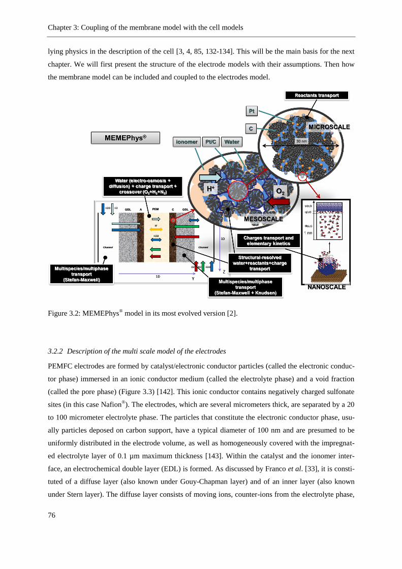
Chapter 3: Coupling of the membrane model with the cell models
76
lying physics in the description of the cell [3, 4, 85, 132-134]. This will be the main basis for the next
chapter. We will first present the structure of the electrode models with their assumptions. Then how
the membrane model can be included and coupled to the electrodes model.
Figure 3.2: MEMEPhys® model in its most evolved version [2].
3.2.2 Description of the multi scale model of the electrodes
PEMFC electrodes are formed by catalyst/electronic conductor particles (called the electronic conduc-
tor phase) immersed in an ionic conductor medium (called the electrolyte phase) and a void fraction
(called the pore phase) (Figure 3.3) [142]. This ionic conductor contains negatively charged sulfonate
sites (in this case Nafion®). The electrodes, which are several micrometers thick, are separated by a 20
to 100 micrometer electrolyte phase. The particles that constitute the electronic conductor phase, usu-
ally particles deposed on carbon support, have a typical diameter of 100 nm and are presumed to be
uniformly distributed in the electrode volume, as well as homogeneously covered with the impregnat-
ed electrolyte layer of 0.1 µm maximum thickness [143]. Within the catalyst and the ionomer inter-
face, an electrochemical double layer (EDL) is formed. As discussed by Franco et al. [33], it is consti-
tuted of a diffuse layer (also known under Gouy-Chapman layer) and of an inner layer (also known
under Stern layer). The diffuse layer consists of moving ions, counter-ions from the electrolyte phase,
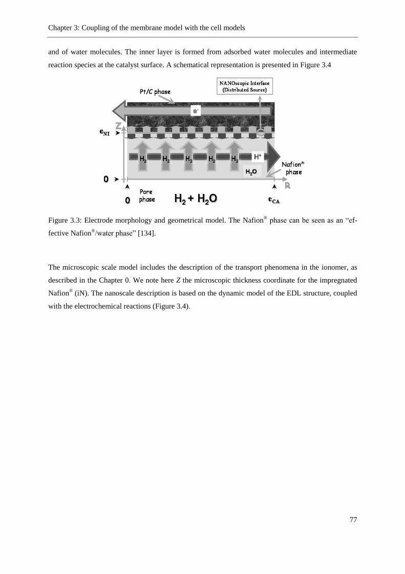
Chapter 3: Coupling of the membrane model with the cell models
77
and of water molecules. The inner layer is formed from adsorbed water molecules and intermediate
reaction species at the catalyst surface. A schematical representation is presented in Figure 3.4
Figure 3.3: Electrode morphology and geometrical model. The Nafion® phase can be seen as an “ef-
fective Nafion®/water phase” [134].
The microscopic scale model includes the description of the transport phenomena in the ionomer, as
described in the Chapter 0. We note here Z the microscopic thickness coordinate for the impregnated
Nafion® (iN). The nanoscale description is based on the dynamic model of the EDL structure, coupled
with the electrochemical reactions (Figure 3.4).

Chapter 3: Coupling of the membrane model with the cell models
78
Figure 3.4: Schematic representation of the non-equilibrium EDL model within MEMEPhys®. Exam-
ple of the anodic case: The hydrogen species arrives to the inner layer where the electron transfer reac-
tion takes place. The proton species is produced at x = L and evacuated through x = 0. (the eventual
contamination by CO and H2S pollutants is also shown but they are not treated in this PhD thesis
work).
Nanoscale model: diffuse layer – In this layer, diffusion and electro-migration transport phenomena
are assumed to occur. The species which are present can be either non-charged (e.g. oxygen or hydro-
gen) or charged (e.g. proton).
In the case of non-charged species, the diffusion process is assumed to be Fickian. Thus we use Equa-
tion 2.22 for the calculation of the concentrations in the diffuse layer. Regarding the low thickness of
the iN (about 10 nm), we consider no Bruggeman correction in the equation of diffusion, as the struc-
ture effect is assumed here as negligible.
In the membrane, the electroneutrality is respected, but in the vicinity of the catalyst, protons are pro-
duced (anode side) or consumed (cathode side). This induces an ionic potential spatial heterogeneity in
the diffuse layer within the iN. Thus the transport of proton will result from two contributions, one due
to the diffusion effect, and the other one to the electromigration effect. The proton are considered as
punctual (diluted solution theory), so that interparticle electrical interactions can be neglected.
Nanoscale model: inner layer – In MEMEPhys® inner layer approach we consider the presence in the
layer of:
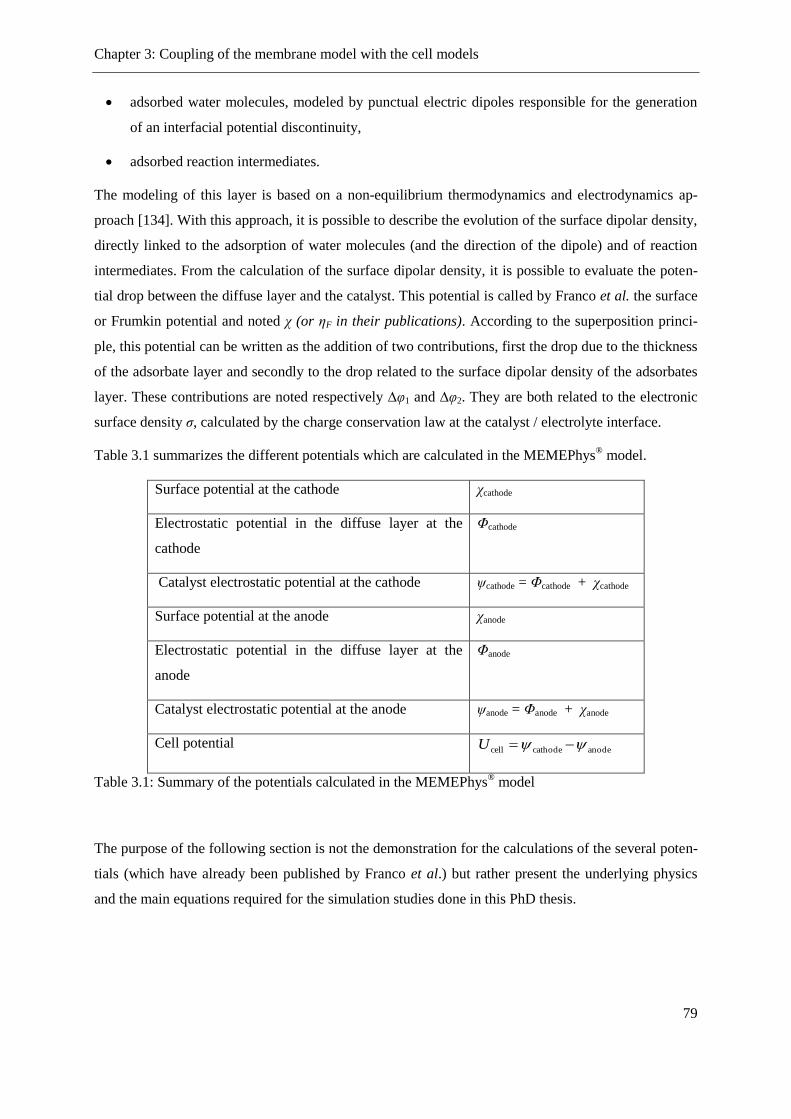
Chapter 3: Coupling of the membrane model with the cell models
79
adsorbed water molecules, modeled by punctual electric dipoles responsible for the generation
of an interfacial potential discontinuity,
adsorbed reaction intermediates.
The modeling of this layer is based on a non-equilibrium thermodynamics and electrodynamics ap-
proach [134]. With this approach, it is possible to describe the evolution of the surface dipolar density,
directly linked to the adsorption of water molecules (and the direction of the dipole) and of reaction
intermediates. From the calculation of the surface dipolar density, it is possible to evaluate the poten-
tial drop between the diffuse layer and the catalyst. This potential is called by Franco et al. the surface
or Frumkin potential and noted χ (or ηF in their publications). According to the superposition princi-
ple, this potential can be written as the addition of two contributions, first the drop due to the thickness
of the adsorbate layer and secondly to the drop related to the surface dipolar density of the adsorbates
layer. These contributions are noted respectively ∆φ1 and ∆φ2. They are both related to the electronic
surface density σ, calculated by the charge conservation law at the catalyst / electrolyte interface.
Table 3.1 summarizes the different potentials which are calculated in the MEMEPhys® model.
Surface potential at the cathode χcathode
Electrostatic potential in the diffuse layer at the
cathode
Φcathode
Catalyst electrostatic potential at the cathode ψcathode = Φcathode + χcathode
Surface potential at the anode χanode
Electrostatic potential in the diffuse layer at the
anode
Φanode
Catalyst electrostatic potential at the anode ψanode = Φanode + χanode
Cell potential anodecathodecell U
Table 3.1: Summary of the potentials calculated in the MEMEPhys® model
The purpose of the following section is not the demonstration for the calculations of the several poten-
tials (which have already been published by Franco et al.) but rather present the underlying physics
and the main equations required for the simulation studies done in this PhD thesis.

Chapter 3: Coupling of the membrane model with the cell models
80
3.2.3 Calculation of the potential in the MEMEPhys® approach
3.2.3.1 Calculation of the potential in the diffuse layer
In the anode catalyst layer, protons are produced. In the vicinity of the catalyst sites, hydrogen mole-
cules adsorb on the platinum surface and split into protons, which stay in the ionomer phase of the
catalyst and electrons, which are conducted to the cathode through the carbon phase. As the protons
are in the Nafion® phase and the electrons in the metallic phase, locally the electroneutrality of the
ionomer phase cannot be assumed. An electrostatic potential distribution is induced in the electrolyte
at the vicinity of the catalyst. This potential distribution is calculated through the numerical resolution
of Poisson’s equation,
²
²· SAH
DL x
ΦCC
F
,
3.1
where εDL is the electric permittivity in the diffuse layer, HC the concentration of protons and SAC
the concentration of sulfonic acid groups. Indeed far from the platinum surface, the electroneutrality is
respected and thus the concentrations of sulfonic acid groups and protons are equal [134].
This electrostatic potential is strongly related to the transport of protons, assumed to be governed by
the Nernst-Planck equation,
²
²·····
·²
²·
HH
H
H
H
H
H
x
ΦCD
x
Φ
x
CD
TR
F
x
CD
t
C
.
3.2
For the coupled solution of Equations 3.1 and 3.2, the used boundary conditions are for the anode side
an electrical potential set to 0, and at the cathode side, the electrical potential value is set as the value
at the boundary between the membrane and the cathode as calculated by the membrane model (see
Section 3.5.3.3).
3.2.3.2 Calculation of the electronic surface density
As previously mentioned in Section 3.2.2, the electronic surface density value is a key parameter, as it
is involved in the calculation of the surface potential of the catalyst. By writing a charge conservation
law at the catalyst / electrolyte interface, we obtain
Anode case ),(),(
),(FarA trJtrJ
t
tr
,
3.3
Cathode case ),(),(
),(FarC trJtrJ
t
tr
,
3.4

Chapter 3: Coupling of the membrane model with the cell models
81
where J(r,t) is the local electronic current density at the catalyst surface, JFar(r,t) are the faradic current
at the anode or cathode side. These current are linked to the electrochemical reaction rate which will
be presented later in Section 3.2.4.1 and Section 3.2.4.2.
3.2.3.3 Calculation of the catalyst surface potential
As mentioned in Section 3.2.2, the surface potential can be split into two contributions due to different
physical phenomena both related to the electronic surface density (see Section 3.2.3.2).
The first contribution is due to the thickness of the adsorbed water layer. If we consider the closed
surface including the inner layer and the charge included in this surface noted as σ, we can write the
Gauss’s law in order to get the electric field at the surface as
CL
),(),(
tr
x
trΦ
,
3.5
where εDL is the electric permittivity in the inner layer.
Regarding the low thickness of the inner layer, Equation 3.5 can be reduced to
d
tr·
),(
CL
1
,
3.6
where d is the thickness of the inner layer.
From Equation 3.6, we have the first contribution to the surface potential. The second one is calculated
explaining the dipolar nature of water molecule adsorbed at the catalyst surface.
The water layer is considered as a layer of punctual dipoles, the interfacial potential drop can thus be
calculated by
DL
2
),(
tr ,
3.7
where Γ is the dipolar surface density.
We need to establish an analytical expression for Γ. For this, Franco used the two states hypothesis for
the description of the adsorption of water molecule. A water molecule can either be adsorbed with the
hydrogen atoms oriented toward the catalyst surface (state 1) or with the lone pairs of water toward the
catalyst surface (state 2) [134]. It is possible to express the dipolar surface density as
21·),( nntr , 3.8
where ni is the number of diploes per unit of area in the state 1 or 2. The objective is now to quantify

Chapter 3: Coupling of the membrane model with the cell models
82
the amount of water in each state.
This is possible through the description of the water adsorption step at the catalyst surface (Reaction
3.1).
Water adsorption H2O + Pt H2O–Pt
Reaction 3.1
Two orientations are possible and the mass action law gives
TR
GGG
an
n iec
s ·exp
·
01,
01,
01,
OH
1
2
,
3.9
TR
GGG
an
n iec
s ·exp
·
02,
02,
02,
OH
2
2
,
3.10
where ns is the number of free sites per unit area of the metallic phase, 0
icG , , 0
ieG , and 0
iiG , are respec-
tively the dipolar chemical adsorption energy, the dipolar electrostatic adsorption energy and the dipo-
lar interaction adsorption energy for the adsorption in the state i (state 1 or 2) and a is the activity of
water.
Knowing the adsorption energy, it is possible to calculate the ni and thus the surface potential. Franco
demonstrated that the coverage of both state can be calculated through
)·exp(
2·· OH1 2
A
ann s , 3.11
)·exp(
2·· OH2 2
A
ann s , 3.12
where X is the solution to the transcendental equation
··
)·cosh(·
*
)·sinh(
OH2
Aan
n
A
s
,
3.13
where n* is the sum of free sites and sites covered by intermediate reaction species per unit area of the
metallic phase,
··CL
3d ,
DL··2
3
and 2
3
·
··
dTk .
The combination of Equations 3.7, 3.8, 3.11 and 3.12 leads to
DL
OH
2
)·sinh(···2
anA s.
3.14
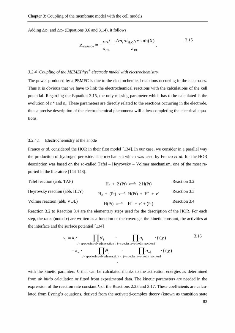
Chapter 3: Coupling of the membrane model with the cell models
83
Adding ∆φ1 and ∆φ2 (Equations 3.6 and 3.14), it follows
DL
OH
CL
electrode
)·sinh(····2
anAd s.
3.15
3.2.4 Coupling of the MEMEPhys® electrode model with electrochemistry
The power produced by a PEMFC is due to the electrochemical reactions occurring in the electrodes.
Thus it is obvious that we have to link the electrochemical reactions with the calculations of the cell
potential. Regarding the Equation 3.15, the only missing parameter which has to be calculated is the
evolution of n* and ns. These parameters are directly related to the reactions occurring in the electrode,
thus a precise description of the electrochemical phenomena will allow completing the electrical equa-
tions.
3.2.4.1 Electrochemistry at the anode
Franco et al. considered the HOR in their first model [134]. In our case, we consider in a parallel way
the production of hydrogen peroxide. The mechanism which was used by Franco et al. for the HOR
description was based on the so-called Tafel – Heyrovsky – Volmer mechanism, one of the most re-
ported in the literature [144-148].
Tafel reaction (abb. TAF) H2 + 2 (Pt) 2 H(Pt)
Reaction 3.2
Heyrovsky reaction (abb. HEY) H2 + (Pt) H(Pt) + H
+ + e
-
Reaction 3.3
Volmer reaction (abb. VOL) H(Pt) H
+ + e
- + (Pt)
Reaction 3.4
Reaction 3.2 to Reaction 3.4 are the elementary steps used for the description of the HOR. For each
step, the rates (noted r) are written as a function of the coverage, the kinetic constant, the activities at
the interface and the surface potential [134]
)(···
)(···
ireaction in involved species i-reaction in involved species
ireaction in involved species ireaction in involved species
fak
fakv
j
i
j
ji
j
i
j
jii
.
3.16
with the kinetic paramters ki that can be calculated thanks to the activation energies as determined
from ab initio calculation or fitted from experimental data. The kinetic parameters are needed in the
expression of the reaction rate constant ki of the Reactions 2.25 and 3.17. These coefficients are calcu-
lated from Eyring’s equations, derived from the activated-complex theory (known as transition state
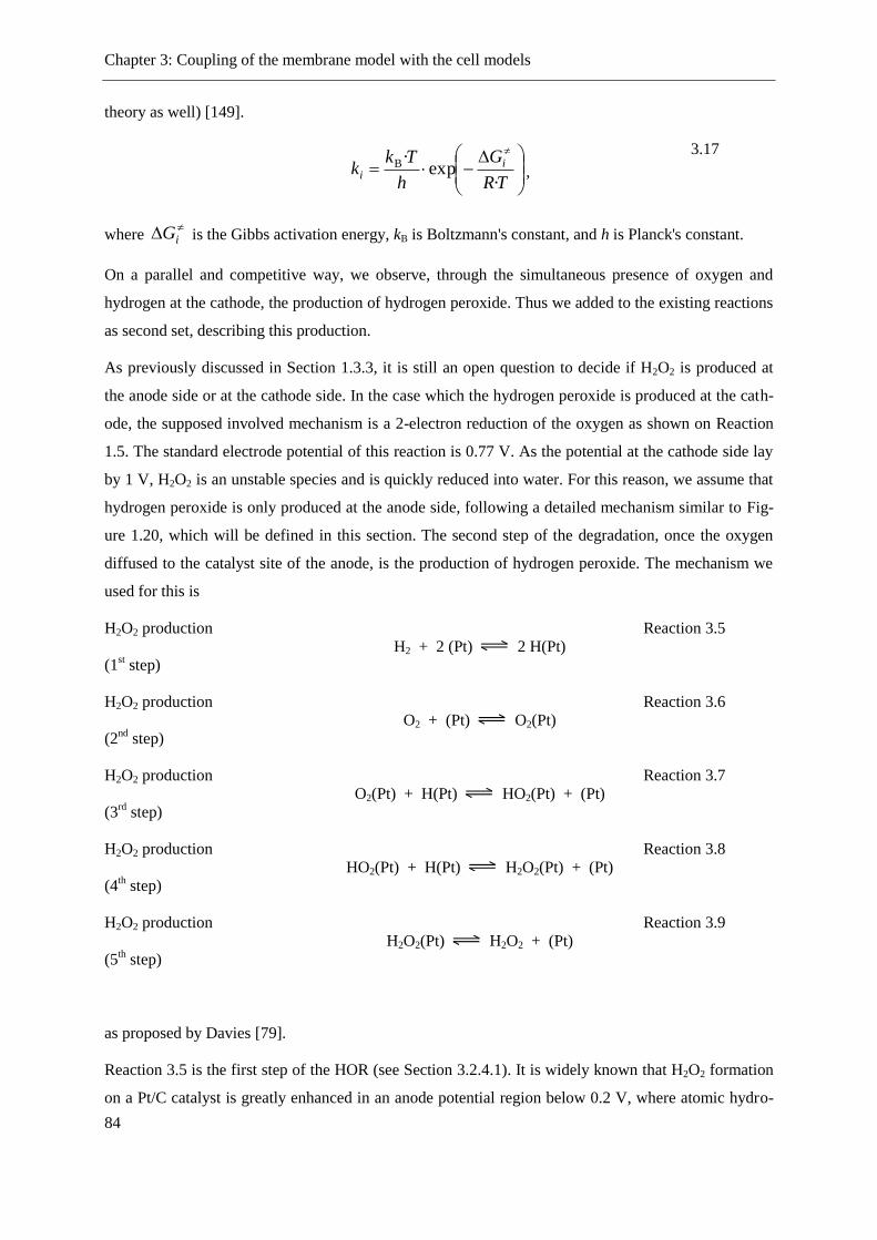
Chapter 3: Coupling of the membrane model with the cell models
84
theory as well) [149].
TR
G
h
Tkk i
i·
exp·B
,
3.17
where iG is the Gibbs activation energy, kB is Boltzmann's constant, and h is Planck's constant.
On a parallel and competitive way, we observe, through the simultaneous presence of oxygen and
hydrogen at the cathode, the production of hydrogen peroxide. Thus we added to the existing reactions
as second set, describing this production.
As previously discussed in Section 1.3.3, it is still an open question to decide if H2O2 is produced at
the anode side or at the cathode side. In the case which the hydrogen peroxide is produced at the cath-
ode, the supposed involved mechanism is a 2-electron reduction of the oxygen as shown on Reaction
1.5. The standard electrode potential of this reaction is 0.77 V. As the potential at the cathode side lay
by 1 V, H2O2 is an unstable species and is quickly reduced into water. For this reason, we assume that
hydrogen peroxide is only produced at the anode side, following a detailed mechanism similar to Fig-
ure 1.20, which will be defined in this section. The second step of the degradation, once the oxygen
diffused to the catalyst site of the anode, is the production of hydrogen peroxide. The mechanism we
used for this is
H2O2 production
(1st step)
H2 + 2 (Pt) 2 H(Pt) Reaction 3.5
H2O2 production
(2nd
step) O2 + (Pt) O2(Pt)
Reaction 3.6
H2O2 production
(3rd
step) O2(Pt) + H(Pt) HO2(Pt) + (Pt)
Reaction 3.7
H2O2 production
(4th step)
HO2(Pt) + H(Pt) H2O2(Pt) + (Pt) Reaction 3.8
H2O2 production
(5th step)
H2O2(Pt) H2O2 + (Pt) Reaction 3.9
as proposed by Davies [79].
Reaction 3.5 is the first step of the HOR (see Section 3.2.4.1). It is widely known that H2O2 formation
on a Pt/C catalyst is greatly enhanced in an anode potential region below 0.2 V, where atomic hydro-
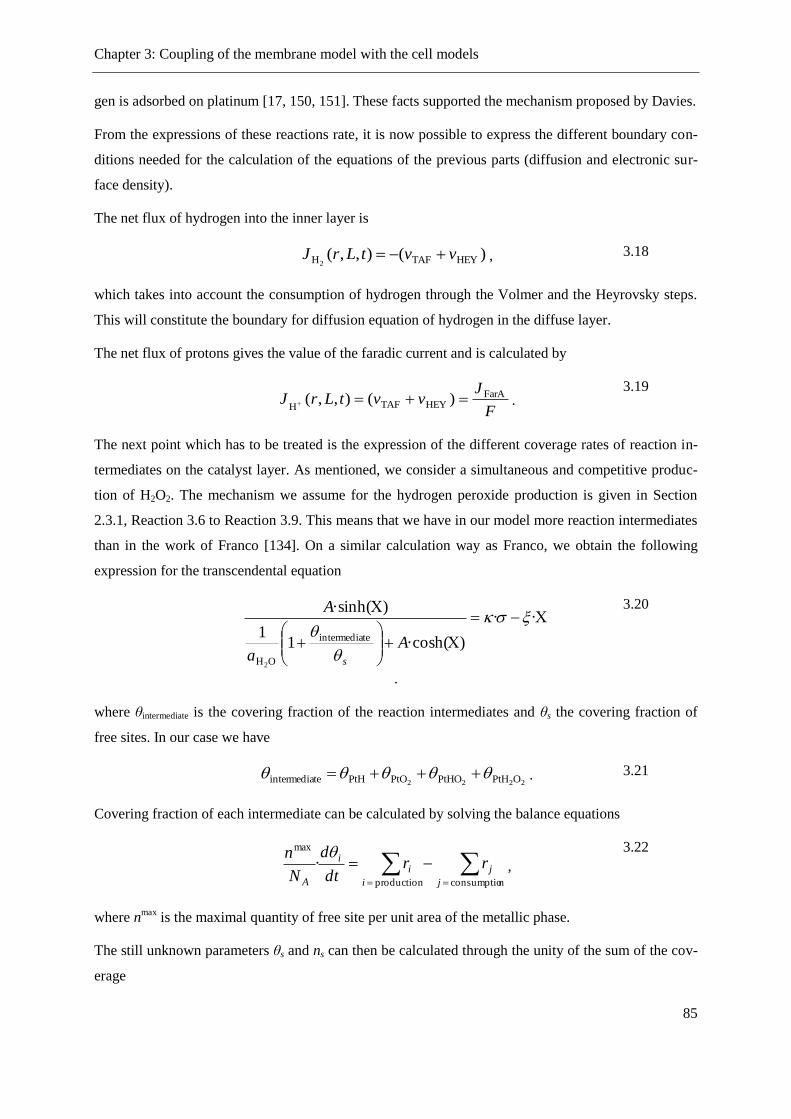
Chapter 3: Coupling of the membrane model with the cell models
85
gen is adsorbed on platinum [17, 150, 151]. These facts supported the mechanism proposed by Davies.
From the expressions of these reactions rate, it is now possible to express the different boundary con-
ditions needed for the calculation of the equations of the previous parts (diffusion and electronic sur-
face density).
The net flux of hydrogen into the inner layer is
)(),,( HEYTAFH2vvtLrJ , 3.18
which takes into account the consumption of hydrogen through the Volmer and the Heyrovsky steps.
This will constitute the boundary for diffusion equation of hydrogen in the diffuse layer.
The net flux of protons gives the value of the faradic current and is calculated by
F
JvvtLrJ FarA
HEYTAFH)(),,( .
3.19
The next point which has to be treated is the expression of the different coverage rates of reaction in-
termediates on the catalyst layer. As mentioned, we consider a simultaneous and competitive produc-
tion of H2O2. The mechanism we assume for the hydrogen peroxide production is given in Section
2.3.1, Reaction 3.6 to Reaction 3.9. This means that we have in our model more reaction intermediates
than in the work of Franco [134]. On a similar calculation way as Franco, we obtain the following
expression for the transcendental equation
··
)·cosh(11
)·sinh(
teintermedia
OH2
A
a
A
s
.
3.20
where θintermediate is the covering fraction of the reaction intermediates and θs the covering fraction of
free sites. In our case we have
2222 OPtHPtHOPtOPtHteintermedia . 3.21
Covering fraction of each intermediate can be calculated by solving the balance equations
nconsumptio production
max
·j
j
i
ii
A
rrdt
d
N
n ,
3.22
where nmax
is the maximal quantity of free site per unit area of the metallic phase.
The still unknown parameters θs and ns can then be calculated through the unity of the sum of the cov-
erage

Chapter 3: Coupling of the membrane model with the cell models
86
1
max
21entermediat
n
nnis and
3.23
ns = θs · nmax
. 3.24
The coupling between the transport model and the electrochemical model in the electrode is now com-
plete for the anode and it is possible to calculate the anodic potential.
3.2.4.2 Electrochemistry at the cathode
On a similar way as for the anode, elementary kinetic steps are written for the ORR. We use here the
model proposed by Franco, as we consider no parasitic reaction at the cathode side [134]. The mecha-
nism which is assumed was proposed by Damjanovic and is [152]
ORR Reaction 1 O2 + 2 (Pt) 2 O(Pt)
Reaction 3.10
ORR Reaction 2 O(Pt) + H
+ + e
- OH(Pt)
Reaction 3.11
ORR Reaction 3 O2 + H
+ + (Pt) + e
- O2H(Pt)
Reaction 3.12
ORR Reaction 4 O2H(Pt) + H2O + 2 (Pt) 3 OH(Pt)
Reaction 3.13
ORR Reaction 5 OH(Pt) + H
+ + e
- H2O + (Pt)
Reaction 3.14
(ab initio –based mechanisms can be also be implemented instead, as recently published by Ferreira de
Morais et al. [153]).
In the cathode case, we write the different fluxes as function of the reaction rates of the ORR mecha-
nism.
The net flux of oxygen into the inner layer is
Dmj1O ),,(
2vtLrJ , 3.25
which takes into account the consumption of hydrogen through Volmer and Heyrovsky steps. This
will constitute the boundary for diffusion equation of hydrogen in the diffuse layer
The net flux of protons gives the value of the faradic current and is calculated by
F
JvvtLrJ FarC
Dmj3Dmj1H)(),,( .
3.26
As we wrote the transcendental equation on a generic way, this remains unchanged. Only the expres-
sion of the reaction intermediates is modified as
PtOHPtHOteintermedia 2
. 3.27
The missing coverage rates can easily be computed on a similar way as in the anodic case using Equa-
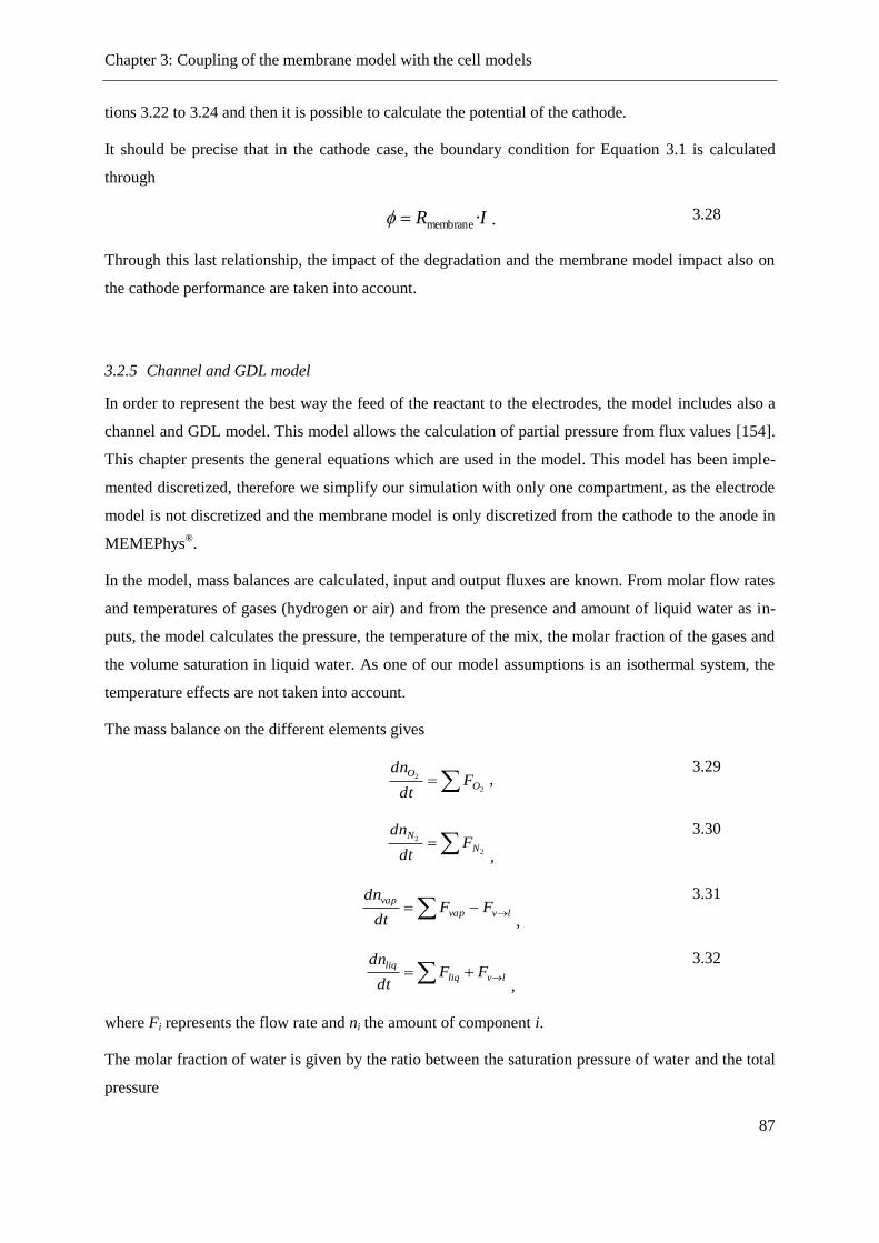
Chapter 3: Coupling of the membrane model with the cell models
87
tions 3.22 to 3.24 and then it is possible to calculate the potential of the cathode.
It should be precise that in the cathode case, the boundary condition for Equation 3.1 is calculated
through
IR ·membrane . 3.28
Through this last relationship, the impact of the degradation and the membrane model impact also on
the cathode performance are taken into account.
3.2.5 Channel and GDL model
In order to represent the best way the feed of the reactant to the electrodes, the model includes also a
channel and GDL model. This model allows the calculation of partial pressure from flux values [154].
This chapter presents the general equations which are used in the model. This model has been imple-
mented discretized, therefore we simplify our simulation with only one compartment, as the electrode
model is not discretized and the membrane model is only discretized from the cathode to the anode in
MEMEPhys®.
In the model, mass balances are calculated, input and output fluxes are known. From molar flow rates
and temperatures of gases (hydrogen or air) and from the presence and amount of liquid water as in-
puts, the model calculates the pressure, the temperature of the mix, the molar fraction of the gases and
the volume saturation in liquid water. As one of our model assumptions is an isothermal system, the
temperature effects are not taken into account.
The mass balance on the different elements gives
2
2
O
OF
dt
dn,
3.29
2
2
N
NF
dt
dn
,
3.30
lvvap
vapFF
dt
dn
,
3.31
lvliq
liqFF
dt
dn
,
3.32
where Fi represents the flow rate and ni the amount of component i.
The molar fraction of water is given by the ratio between the saturation pressure of water and the total
pressure

Chapter 3: Coupling of the membrane model with the cell models
88
P
TPX sat
sat
)( .
3.33
22 NOvap
vap
vapnnn
nX
3.34
where X represents the molar fraction in the gaseous phase.
In order to calculate the pressure of the different gas components, the following equations are used:
liq
liqliq
liq
MnV
· ,
3.35
liqgas VVV
, 3.36
gaz
vapNO
gazV
TRnnnP
22
,
3.37
)(sJkP Pccap , 3.38
capgasliq PPP 3.39
where Vi is the volume of phase i, ni is the amount of substance i, Pi the pressure of phase i and J(s)
the Leverett J-function, a dimensionless function of water saturation describing the capillary pressure
[153].
From these results on the channel, the model then calculates the concentration of the different gas
components in the pore of the GDL, which are reused in the mass balance equation of the electrode
model.
3.3 Physics underlying in the electrode model of DENIS
3.3.1 Presentation of the model
Bessler and co-workers develop the DENIS model since 2003. Even if the initial conception of DENIS
was designed in a way that simulations of solid-oxide fuel cell (SOFC) were possible, the modularity
of the C-programmed model and the similarities in the architecture of a SOFC and PEMFC made it
possible to adapt the model to the PEMFC system [137, 155]. The following chapter will present the
DENIS model, the way it treats the electrodes and the transport phenomena.

Chapter 3: Coupling of the membrane model with the cell models
89
3.3.2 Calculation of the cell potential in DENIS
3.3.2.1 General aspects
As in MEMEPhys®, the calculation of the cell voltage in DENIS is given by the difference of the elec-
tric potentials in the cathode and in the anode. This allows to the model to calculate on a quasi 2D way
the distribution of the gas-phase species, the current, the potential, as well as the pressure and the flow
velocities. We will recall here the main equations needed for the computation of the cell potential.
In Figure 3.6, we present the global architecture of DENIS. For a better understanding how the cell
potential is calculated, we plot schematically the contribution of anode, cathode and electrolyte on the
cell voltage in Figure 3.7.
Like in the MEMEPhys® approach, the cell voltage is calculated after
ancacell U , 3.40
the difference will be in the calculation of the electrode potentials.
The formalism we used here is the one as in the original work of Bessler et al. [155]. Indeed so that
the reader could refer to the original work, we keep the consistency in the notation. This explains why
some symbols conflicts may occur with the previous parts.
The driving equations used in the DENIS model for the calculation of every contribution of the cell
voltage (as displayed in Figure 3.7) are given in Figure 3.5.

Chapter 3: Coupling of the membrane model with the cell models
90
Figure 3.5: Summary of the governing equations of the DENIS model [155].

Chapter 3: Coupling of the membrane model with electrode and cell models
91
Figure 3.6: Schematic representation of the 2D model DENIS
Figure 3.7: Detailed contributions of each cell part to the calculation of the voltage
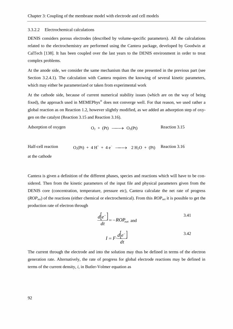
Chapter 3: Coupling of the membrane model with electrode and cell models
92
3.3.2.2 Electrochemical calculations
DENIS considers porous electrodes (described by volume-specific parameters). All the calculations
related to the electrochemistry are performed using the Cantera package, developed by Goodwin at
CalTech [138]. It has been coupled over the last years to the DENIS environment in order to treat
complex problems.
At the anode side, we consider the same mechanism than the one presented in the previous part (see
Section 3.2.4.1). The calculation with Cantera requires the knowing of several kinetic parameters,
which may either be parameterized or taken from experimental work
At the cathode side, because of current numerical stability issues (which are on the way of being
fixed), the approach used in MEMEPhys® does not converge well. For that reason, we used rather a
global reaction as on Reaction 1.2, however slightly modified, as we added an adsorption step of oxy-
gen on the catalyst (Reaction 3.15 and Reaction 3.16).
Adsorption of oxygen O2 + (Pt) O2(Pt) Reaction 3.15
Half-cell reaction
at the cathode
O2(Pt) + 4 H+ + 4 e
− 2 H2O + (Pt) Reaction 3.16
Cantera is given a definition of the different phases, species and reactions which will have to be con-
sidered. Then from the kinetic parameters of the input file and physical parameters given from the
DENIS core (concentration, temperature, pressure etc), Cantera calculate the net rate of progress
(ROPnet) of the reactions (either chemical or electrochemical). From this ROPnet it is possible to get the
production rate of electron through
netROP
dt
ed
and
3.41
dt
edFI
·
3.42
The current through the electrode and into the solution may thus be defined in terms of the electron
generation rate. Alternatively, the rate of progress for global electrode reactions may be defined in
terms of the current density, i, in Butler-Volmer equation as
Chapter 3: Coupling of the membrane model with electrode and cell models
93
TR
F
TR
Fii ss
·
··βexp
·
·)·β1(exp·
ee
0
3.43
where i0 is the exchange current density, βe is the symmetry factor for the transition state and ηs is the
overpotential (represents the departure from the equilibrium potential at the specific conditions of the
electrode).
3.3.3 Gas transport and channel model in DENIS
In this section, the transport models of mass and charge are described. We are using a quasi-1D+1D-
description that covers two length scales, as shown in Figure 3.6:
gas-phase flow in the gas chamber above the PEMFC electrodes (mm–cm scale, x dimension)
gas-phase and charge transport within the porous electrodes (µm–mm scale, y dimension)
Every individual scale is modeled in one dimension, and the scales are coupled through appropriate
boundary conditions. This allows capturing all relevant physicochemical processes, while keeping
computational cost to a reasonable level as compared to a full 2D model [155].
Gas-phase flow is modeled using 1D representation of the Navier–Stokes equations. The porous elec-
trodes are treated as continuum of the three involved phases gas-phase, electrode and electrolyte. The
transport within each of the three phases (gas species, electrons and oxygen ions, respectively) is de-
scribed using effective transport coefficients. Gas-phase transport in the porous electrodes is modeled
by two parallel transport pathways: Stefan–Maxwell diffusion and Darcy viscous flow. For the diffu-
sion pathway, modified Bosanquet diffusion coefficients are used that account for both, free-molecular
and Knudsen diffusion.
The transport of the gaseous reactants and products takes place through convection and diffusion in
the gas chamber above each electrode. These gas transport situations are modeled with one dimension-
al representations of the transient Navier–Stokes equations (conservation of mass – Equation 3.44,
momentum – Equation 3.45 and species-Equation 3.46).
ii Ms
A
P
x
v)(
t
cha
cha
chachem
,
3.44
wcha
chah)(
A
P
x
p
x
vv)(
t
v
,
3.45
ii
iii MsA
P
x
j
x
vY
t
Y cha
cha
chachem
diff)()(
3.46

Chapter 3: Coupling of the membrane model with electrode and cell models
94
.
As previously mentioned, DENIS was first designed for simulations of SOFC technology [135, 136,
155, 156]. Even if the role of the electrodes, electrolyte and gas channel remains the same compared to
PEFC technology, one aspect is different comparing both cell designs. In a PEMFC a GDL is needed
for a good gas supply at the catalyst layer and a good evacuation of the produced liquid water at the
cathode side (see Section 1.1.2). In SOFC technology, a current collector is needed to drive the elec-
tron outside out the cathode to the anode. This can be seen as a conductive porous structure, defined
through porosity, tortuosity and thickness. Even if from its use it differs from the GDL, its properties
can be adapted so that it is representative of a GDL. The only assumption we have to make is the non-
presence of liquid water in the porous media representing the GDL. The modeling of the transport
phenomena is the same; only the characteristics of the media are modified.
3.4 Comparison MEMEPhys® / DENIS electrode models
This part summarizes the properties of each model as used in this PhD thesis work, their common
points and their differences. For clarity purposes, the points we discussed are presented in Table 3.2.
Property DENIS MEMEPhys®
Programming
language
C C, Matlab / Simulink
Solver Limex [140] Simulink ode23s Simulink
Physical approach Equilibrium thermodynamics Non-equilibrium thermodynamics
Electrochemistry
Anode
Butler-Volmer-based elementary
kinetics Production of H2O2
Ab initio-based elementary kinetics
Production of H2O2
Nanoscale electrochemical double layer
structure explicity simulated
Electrochemistry
Cathode
Butler-Volmer-based global kinetics Ab initio-based elementary kinetics
Nanoscale electrochemical double layer
structure explicitly simulated
Discretization Two dimensional discretization (1D
+ 1D)
Along the gas channel
Membrane discretized (1D + 1D)
Local discretization inside the
electrodes carbon agglomerates

Chapter 3: Coupling of the membrane model with electrode and cell models
95
In transversal direction (from
gas channel cathode to gas
channel anode)
Discretization along the
GDL+MEA thickness
Scaling Multi-scale model:
description of gas transport
along the channel at the
macro-scale
description of transport phe-
nomena in the electrodes
and the electrolyte at a mi-
cro-scale
Multi-scale model:
description of gas and water
transport in the channel and the
GDL at a macro-scale
description of nano-scale reaction
and transport phenomena in the
vicinity of the catalyst
description of transport phenom-
ena in the electrodes and the
electrolyte at a micro-scale
Table 3.2: DENIS – MEMEPhys® models: comparison of the general features as used in this PhD
thesis work.
We had the opportunity to work on a parallel way with two codes. Both are complex and advanced;
therefore they differ in some of their assumptions and approach. They are both designed on a modular
way, so to make easier any modification on an aspect of the code. Thanks that, it is possible to modify
for example the physics used for the transport phenomena in the gas phase without having to change
anything in the rest of the code. This modularity was the key, which allowed us to reuse the membrane
module in both code. We just had to replace the previous membrane model by the new one and couple
it to the rest of the cell. Within the module itself it is also possible to perform modifications without
changing the rest of the code.
DENIS offers possibilities, for example in the investigation of gas distribution profiles on electrode
surfaces and thus a screening of the areas of the electrode where the electrochemical activity is not
optimal. Such a study has already successfully been done in the case of SOFC [136]. A second point is
that DENIS is programmed in C and does not depend on any commercial software and the drawbacks
linked to their uses. Even if the requirement to program on it is higher than with Matlab for example,
we have a higher flexibility for example in the use of the solver.
MEMEPhys® allows simulating a whole cell. It focuses on a precise description of the electrochemical
double layer at the surface of the catalyst layer [133, 134]. Its strength lies in its physical approach of
the electrochemistry and transport phenomena at multiple scales and in its capabilities to numerically
account for the feedback between the reaction and transport processes and materials aging phenomena:

Chapter 3: Coupling of the membrane model with electrode and cell models
96
Unlike DENIS and most of the other work published in the literature, MEMEPhys® uses, instead of an
top-down modeling approach, a bottom-up approach. The phenomena described at the nano-scale are
the causes of the observation at the upper scales (e.g. any Butler-Volmer equation is used, and ab ini-
tio and microstructural data can be easily integrated). Moreover, the use of non-equilibrium thermody-
namics is justified by the fact that fuel cells are continuously fed by gases at different fluxes, depend-
ing on the demand and thus, cannot really be considered as system in equilibrium.
3.5 Coupling of the membrane model with the electrodes model
3.5.1 Generalities
As the membrane is sandwiched between the anode and the cathode and because of the continuity
principle at the interfaces electrodes / membrane, we have to couple the boundary conditions so that
the definition of several inputs and outputs in the model are consistent.
Electrodes are the locations where the electrochemical reactions required for the current production
take place, and the reactant are fed through the channel and the GDLs. But in the case of the ORR for
example, the proton which are required are produced at the anode and have to diffuse through the
membrane. This means that the electrodes models provide boundary conditions to several equations
computered by the membrane module. Thus the next chapter aims on explaining how the coupling is
made, depending on the simulation environment.
3.5.2 Specifications for the coupling in DENIS
The membrane model was originally developed in C and integrated to the DENIS environment. Thus
no changes or adaptation were required to get the model operating. The several parameters which
could be needed by the module are directly given by the other modules present in DENIS.
This includes:
• The current density, needed for the calculation of the electro-osmotic drag contribution of the
water flux (Equation 2.8)
• The partial pressure of the gases at the anode and the cathode, needed for the application of
Henry’s law (Equation 2.21)
• The production term of each species are driven by the electrochemistry and the resolution of the
diffusion equations through the membrane and degradation are made in the membrane module. Thus a
coupling is needed as well, so that the boundary conditions remain time-dependent.

Chapter 3: Coupling of the membrane model with electrode and cell models
97
3.5.3 Specifications for the coupling in MEMEPhys®
3.5.3.1 General aspect of the membrane module coupling in MEMEPhys®
The C-module is embedded into MEMEPhys® (Matlab / Simulink environment) through the use of an
S-Function (as defined in Section 3.1.3). Thus it is necessary to couple the module to the rest of the
model. The module receives inputs from the module and gives outputs as displayed in Figure 3.8.
Moreover, some light modifications were made, as parameters were computed both in the S-Function
and in the rest of the Simulink model.
Figure 3.8: Coupling the membrane module into MEMEPhys®
3.5.3.2 Inputs from MEMEPhys® to the membrane module
The first information which has to be given to the membrane module is the current density demanded
to the cell. The current density is one of the input parameters when using a MEMEPhys® model. Its
value is then directly fed into the S-Function.
The second parameters which have to be given to the module are the boundary conditions for the
transport equation. For the diffusion of dissolved gases through the membrane thickness (Equation
2.22), the concentrations of dissolved gases at the electrode / membrane interfaces are needed. This is
calculated in DENIS through the expression of Henry’s law (Equation 2.21). In the case of ME-
MEPhys®, this calculation was already implemented in the GDL model. Thus it is possible to feed
directly the value of dissolved gas concentrations into the membrane module. For water transport, the
issue is similar. Equation 2.4 allows the calculation of the evolution of the water content λ along the
membrane. Equations 2.11 and 2.12 are used in DENIS as boundary conditions, based on the value of

Chapter 3: Coupling of the membrane model with electrode and cell models
98
the relative humidity and the production of water from the ORR. As MEMEPhys® describes in the
cathode model the electrochemical phenomena and calculates water balance in the catalyst layer; we
assume that there is no open gas pore at the electrode / membrane interfaces and, as the thickness of
the ionomer is really thin compared to the membrane thickness, the net flux of water in the electrode is
represent the boundary conditions for water flux in the membrane model, as presented in Section
2.2.1.1.
Last, as the hydrogen peroxide is produced at the anode side and but decomposed in the membrane, its
production rate must be given to the membrane module, in order to be taken into account in the mass
balance equation for this component.
3.5.3.3 Outputs from the membrane module to MEMEPhys®
Most of the output we configured are used for post-treatment and are not related to the rest of the
model (evolution of porosity, conductivity, concentration profiles etc.). But some of them represent
parameters in further calculations in the model.
First for the calculation of the potential in the diffuse layer, the membrane resistance is needed (see
Table 3.1). Even if it would have been possible to calculate directly the potential in the membrane
module, our choice was rather using the membrane area specific resistance, so that its value can be
monitored as well.
The second important information delivered by the membrane module is the concentration of dis-
solved gases in the electrodes. We assume a continuity of the concentration of species in an electrode
and in the membrane at y = 0 (cathode side) or y = Lmembrane (anode side). In our model and under our
assumptions, two concentrations are relevant for the electrochemical calculations, the concentration of
hydrogen peroxide and the concentration of dissolved oxygen, both involved in the chemistry of hy-
drogen peroxide formation. For the same reason, fluxes of dissolved gases over membrane boundaries
are required, in order to solve the Fickian diffusion equations in the electrodes.
Last, as the water balance in the electrodes are calculated outside the membrane model (see also Sec-
tion 3.5.3.2), the values of the water content y = 0 (cathode) and y = Lmembrane (anode) are needed, so
that it can be calculated whether the difference of the water content in the electrode is positive or nega-
tive. That will define for example if the membrane dries out (that means water is transferred from the
membrane to the electrode).

Chapter 3: Coupling of the membrane model with electrode and cell models
99
3.6 Summary
In this chapter we have presented the two preexisting cell models and how our membrane model can
be coupled to them. These models are different in the programming and in the physical approach but
through the use of C language for the programming of our membrane, we got a generic module easy to
embed in both environments.
The next chapter will then deal with the parameterization and the possible uses of this model to help in
the comprehension and the interpretation of experimental observables.


Chapter 4: Results and discussion
101
CHAPTER 4
Results and discussion
Le modèle étant établi, il est nécessaire de déterminer les paramètres manquants au fonctionne-
ment complet du modèle. Pour cela, des résultats expérimentaux sont nécessaires.
Dans le cadre de cette thèse, la plupart des expériences utilisées sont extraites de la littérature.
Les paramètres manquants du modèle (constantes cinétiques) peuvent ainsi être évalués, en
comparant les résultats du modèle avec les résultats d’expérience. Chaque étape de la boucle de
dégradation est ainsi paramétrisée et validée expérimentalement. Il s’agit :
- De l’évaluation des constantes cinétiques de l’adsorption de l’oxygène sur le catalyseur à
l’anode lors de la production de peroxyde d’hydrogène.
- De la validation de la cinétique utilisée dans l’étape de décomposition du peroxyde
d’hydrogène en radicaux via les réactions impliquées dans la chimie de Fenton.
- De l’évaluation de la constante cinétique associée à l’étape de scission des chaînes pen-
dantes lors de la dégradation chimique de la membrane.
Cette paramétrisation a été réalisée grâce aux fonctions d’optimisation de MATLAB/Simulink et
assure de la fiabilité du modèle et de l’approche adoptée. Au préalable, le modèle d’électrodes a
été validé grâce à des expériences réalisées au sein de LCPEM au CEA Grenoble.
Nous avons utilisé notre modèle de dégradation avec couplage des électrodes pour différents
modes de fonctionnement et différentes conditions opératoires, représentant diverses applica-
tions pouvant être rencontrées lors du fonctionnement d’une pile à combustible. Le type de
mode opératoire peut par exemple être un fonctionnement sous courant continu ou une varia-
tion périodique des conditions de courant, oscillant entre deux valeurs extrêmes. Différents types
de membranes PFSA ont également été simulées dans des conditions. Selon les réactants utilisés
lors de la synthèse de la membrane, il est possible de produire une grande gamme de membranes
avec masse équivalente et des longueurs de chaînes pendantes variables. En fixant un critère de
fin de vie de pile (dans le cadre de cette étude on a fixé la fin de vie de la pile à une diminution de
5 % du potentiel de cellule inital), le modèle permet de déterminer le temps nécessaire à la cel-
lule. Pour finir, après avoir identifié les paramètres pouvant influer la dégradation chimique,

Chapter 4: Results and discussion
102
une analyse de sensitivité a pour finir été effectuée.
De simulations effectuées à courant constant, nous observons que la dégradation chimique est
moins importante lorsque la densité de courant augmente. La pression ne semble pas avoir
d’effet significatif sur la dégradation chimique, au contraire de la température. En quantifiant la
dégradation chimique en termes de production d’ions fluoride, une augmentation de 10 °C de la
température augmente par deux la dégradation. Une des conséquences de cette dégradation est
une augmentation de la résistance de la membrane. A faibles densités de courant, comme la dé-
gradation chimique est plus sévère, l’augmentation de la résistance de la membranse sera plus
élevée. Cependant, compte tenu de la contribution de la valeur du courant dans le calcul des
pertes ohmiques, l’impact de la dégradation sera moins prononcé lors de l’observation de
l’évolution du potentiel de la cellule. En revanche à densités de courant plus élevées,
l’augmentation de la résistance de la cellule est moindre, mais la valeur élevée du courant im-
plique une augmentation des pertes ohmiques plus élevées. Ce phénomène explique les résultats
observés dans l’étude de la durée de vie de cellule en fixant un critère observable expérimenta-
lement de fin de vie correspondant à une diminution du potentiel de cellule. La durée de vie des
piles sous ces conditions est plus courte à hautes densités de courant qu’à faibles densités de cou-
rant.
En appliquant une densité de courant oscillant entre deux valeurs à une cellule, le modèle
montre que la dégradation chimique observée est une dégradation intermédiaire comprise entre
deux états de référence obtenus lors des simulations à courant constants, ce qui traduit une in-
dépendance de la dégradation chimique à des conditions de cyclage.
En ce qui concerne la nature de la membrane PFSA, le modèle ne montre qu’un impact mineur
sur la dégradation chimique.
Expérimentalement, il a été observé que lorsque la quantité d'ions fer présente dans la cellule est
élevée et dépasse un certain seuil, la dégradation chimique exprimée en termes d'émission d'ions
F- diminue. Eu égard aux différents paramètres que nous pouvons suivre, nous conclûmes qu'un
excès d'ions fer dans la cellule va jouer le rôle de piège à radicaux et ainsi protéger la membrane
des attaques radicalaires.
L'analyse de sensibilité montre que l’aspect déterminant dans le contrôle de la dégradation chi-
mique de membranes PFSA est les conditions expérimentales, notamment la température et
l’humidité relative dans les gaz aux électrodes. Il a également été mis en évidence que la limita-
tion de l’étape de production de peroxyde d’hydrogène à l’anode ne constitue pas un point essen-
tiel dans la dégradation chimique.

Chapter 4: Results and discussion
103
4 Results and discussion
4.1 Introduction
This chapter presents the validation of our model and simulation results obtained within MEMEPhys®
simulation package, for different experimental conditions and membrane type. We will focus our anal-
ysis on the interpretation of several output of the model, as the cell voltage, the membrane resistance
or the cumulative fluoride released for example.
When we simulate the behavior of a cell, we give as inputs parameters which not necessarily define a
stable state for the cell. The models will then first drive the cell to a stable state and consequently ad-
just the parameters. We call this phase the numerical preconditioning phase. It usually takes about 20
simulated hours at the beginning and the relevant part for the study of the chemical degradation is then
beyond these first 20 hours. This effect can be seen in Figure 4.1, where the first 20 h are needed by
the model to reach a steady state.
The second point to be explained is in the calculation of the potential at zero current. OCV is not cal-
culated in MEMEPhys® through Nernst equation but calculated as a potential difference between cath-
ode and anode at zero current. To calculate the cathode potential, the ORR mechanism used in this
PhD thesis (as presented in Reaction 3.10 to Reaction 3.14 in Section 3.2.4.2) is the empirical Damja-
novic’s pathway [152]. Franco showed that the calculation of the cathode potential at zero current with
this mechanism mathematically returns multiple solutions [132]. Because of this we consider here that
a small current density (0.04·10–2
A·cm–2
) is representative of open circuit. As the application of a
non-zero current density will activate the cell, we observe effects on the response of several model
parameters. In Figure 4.1, we plotted the evolution of the relative humidity for two current conditions.
For a 25 cm² geometric area membrane, we applied 0 A and 1 A absolute current. As is can be seen,
the small amount of water produced by applying a non-zero current induces an increase of the relative
humidity. The difference remains not so significant, as the high stoichiometry ensures a quick remov-
ing of the produced water. Figure 4.2 shows the same simulation with decreased stoichiometries. In
that case, the differences are more important. In Figure 4.3, we represented the evolution of the water
content in the membrane for the different current conditions. We see that the membrane contains more
water and consequently will present better proton conductivity. At 0.04 A·cm–2
, the water content is
unbalanced compared to OCV conditions. This will then impact the cell resistance.
To mitigate this problem, we will then in this work perform simulations at high stoichiometry, so that
our low current simulations are close to what would be expect under OCV conditions.
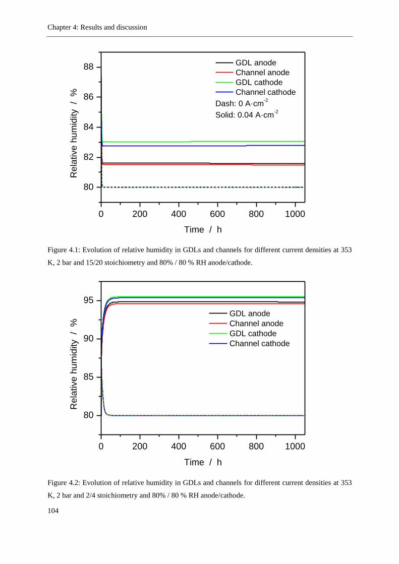
Chapter 4: Results and discussion
104
Figure 4.1: Evolution of relative humidity in GDLs and channels for different current densities at 353
K, 2 bar and 15/20 stoichiometry and 80% / 80 % RH anode/cathode.
Figure 4.2: Evolution of relative humidity in GDLs and channels for different current densities at 353
K, 2 bar and 2/4 stoichiometry and 80% / 80 % RH anode/cathode.
0 200 400 600 800 1000
80
82
84
86
88 GDL anode
Channel anode
GDL cathode
Channel cathode
Dash: 0 A·cm-2
Solid: 0.04 A·cm-2
Re
lative
hu
mid
ity
/ %
Time / h
0 200 400 600 800 1000
80
85
90
95
GDL anode
Channel anode
GDL cathode
Channel cathode
Re
lative
hu
mid
ity
/ %
Time / h

Chapter 4: Results and discussion
105
Figure 4.3: Steady-state water profile in the membrane for different current conditions at 353 K, 2 bar
and 80% / 80 % RH anode/cathode.
4.2 Model parameterization and evaluation
4.2.1 Presentation of the “standard” cell used in the simulations
In a PEMFC, many parameters having an influence on the response of the cell can be controlled. In the
present chapter, we will distinguish the experimental condition parameters from the cell design param-
eters and the stress applied to the cell (we mean here the current load condition, which we separate
from physical experimental parameters). Table 4.1 presents a list of the parameters which can be
viewed as potentially relevant for the degradation of the cell. Some of the parameters have an impact
rather on the cell performance, other on the chemical degradation. For example, it is obvious that if we
increase the platinum load in the electrodes, the performance will be better than for lower load, but
that would not necessarily mean that their impact on the chemical degradation is significant.
Experimental condition Cell design Applied stress
Temperature Membrane thickness Constant current
0.0 0.2 0.4 0.6 0.8 1.0
7
8
9
10
11
12
Anode
OCV
0.04 A·cm-2 low stoich.
0.04 A·cm-2 high stoich.
Position in the membrane / -
Cath
ode
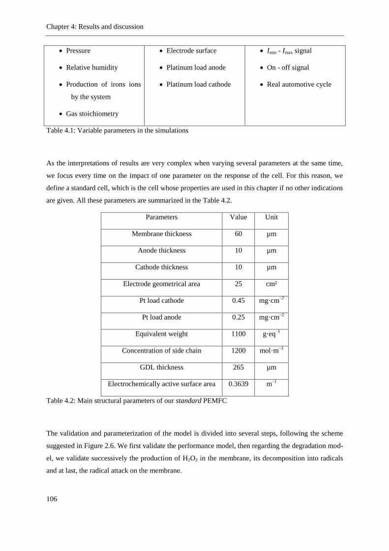
Chapter 4: Results and discussion
106
Pressure
Relative humidity
Production of irons ions
by the system
Gas stoichiometry
Electrode surface
Platinum load anode
Platinum load cathode
Imin - Imax signal
On - off signal
Real automotive cycle
Table 4.1: Variable parameters in the simulations
As the interpretations of results are very complex when varying several parameters at the same time,
we focus every time on the impact of one parameter on the response of the cell. For this reason, we
define a standard cell, which is the cell whose properties are used in this chapter if no other indications
are given. All these parameters are summarized in the Table 4.2.
Parameters Value Unit
Membrane thickness 60 µm
Anode thickness 10 µm
Cathode thickness 10 µm
Electrode geometrical area 25 cm²
Pt load cathode 0.45 mg·cm–2
Pt load anode 0.25 mg·cm–2
Equivalent weight 1100 g·eq–1
Concentration of side chain 1200 mol·m–3
GDL thickness 265 µm
Electrochemically active surface area 0.3639 m–1
Table 4.2: Main structural parameters of our standard PEMFC
The validation and parameterization of the model is divided into several steps, following the scheme
suggested in Figure 2.6. We first validate the performance model, then regarding the degradation mod-
el, we validate successively the production of H2O2 in the membrane, its decomposition into radicals
and at last, the radical attack on the membrane.
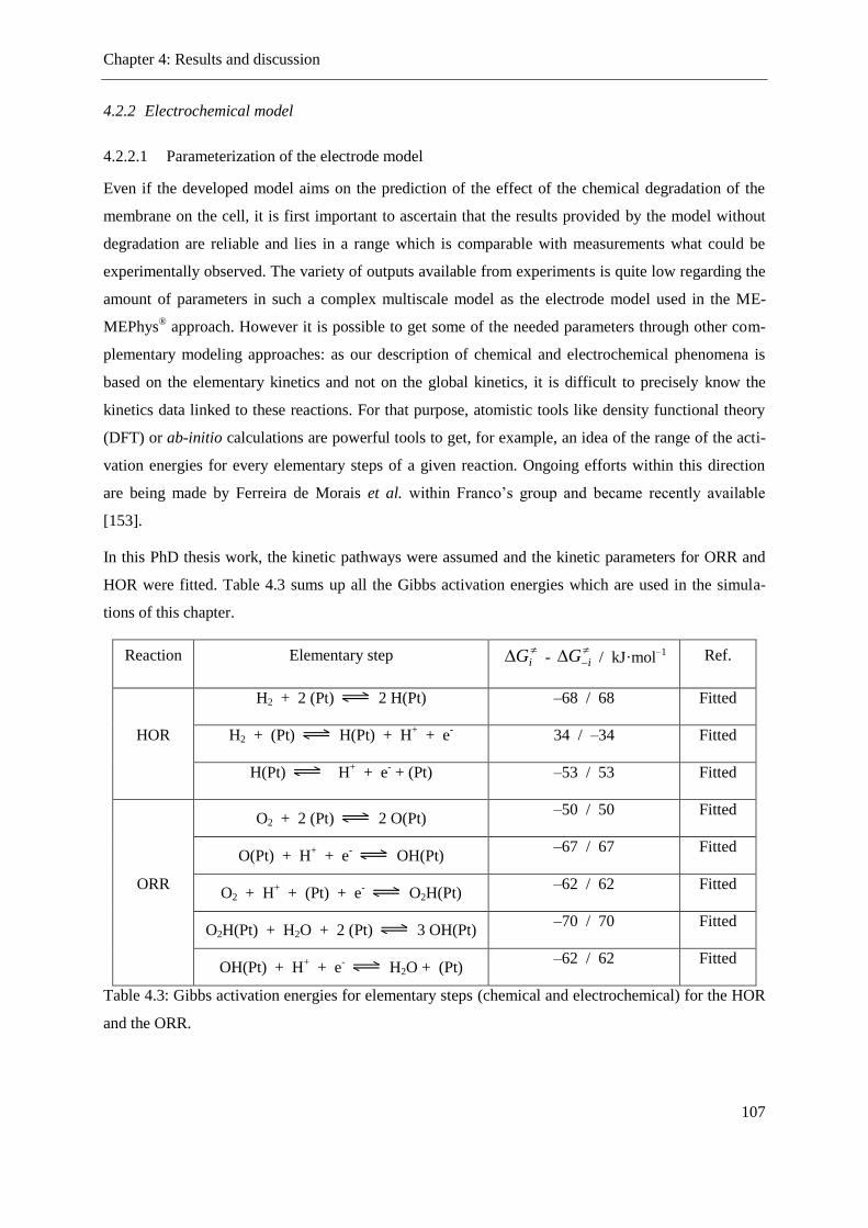
Chapter 4: Results and discussion
107
4.2.2 Electrochemical model
4.2.2.1 Parameterization of the electrode model
Even if the developed model aims on the prediction of the effect of the chemical degradation of the
membrane on the cell, it is first important to ascertain that the results provided by the model without
degradation are reliable and lies in a range which is comparable with measurements what could be
experimentally observed. The variety of outputs available from experiments is quite low regarding the
amount of parameters in such a complex multiscale model as the electrode model used in the ME-
MEPhys® approach. However it is possible to get some of the needed parameters through other com-
plementary modeling approaches: as our description of chemical and electrochemical phenomena is
based on the elementary kinetics and not on the global kinetics, it is difficult to precisely know the
kinetics data linked to these reactions. For that purpose, atomistic tools like density functional theory
(DFT) or ab-initio calculations are powerful tools to get, for example, an idea of the range of the acti-
vation energies for every elementary steps of a given reaction. Ongoing efforts within this direction
are being made by Ferreira de Morais et al. within Franco’s group and became recently available
[153].
In this PhD thesis work, the kinetic pathways were assumed and the kinetic parameters for ORR and
HOR were fitted. Table 4.3 sums up all the Gibbs activation energies which are used in the simula-
tions of this chapter.
Reaction Elementary step iG - iG / kJ·mol
–1 Ref.
HOR
H2 + 2 (Pt) 2 H(Pt) –68 / 68 Fitted
H2 + (Pt) H(Pt) + H+ + e
- 34 / –34 Fitted
H(Pt) H+ + e
- + (Pt) –53 / 53 Fitted
ORR
O2 + 2 (Pt) 2 O(Pt) –50 / 50 Fitted
O(Pt) + H+ + e
- OH(Pt)
–67 / 67 Fitted
O2 + H+ + (Pt) + e
- O2H(Pt)
–62 / 62 Fitted
O2H(Pt) + H2O + 2 (Pt) 3 OH(Pt) –70 / 70 Fitted
OH(Pt) + H+ + e
- H2O + (Pt)
–62 / 62 Fitted
Table 4.3: Gibbs activation energies for elementary steps (chemical and electrochemical) for the HOR
and the ORR.

Chapter 4: Results and discussion
108
4.2.2.2 Experimental setup
The CEA laboratory of fuel cell components, electrolyzers and modeling (LCPEM) is involved in lot
of European projects dealing among other with durability and degradation issues. One of these, named
DECODE, focuses on the comprehension and elucidation of degradation mechanisms in PEMFC with
special focus on the influence of liquid water [40]. We have received experimental results of this pro-
ject at LCPEM from Dr. Escribano. In Table 4.4, the main parameters used during the experiment are
summed up. The MEA used in this project was not Nafion® but Aquivion E79-03, whose molecular
structure is slightly different than the one of Nafion® (see Figure 4.4). Its equivalent weight is 790
g·eq–1
and it is only 30 µm thick.
Figure 4.4: Comparison of the chemical structure of Nafion® (left) and Aquivion (right)
As we first regard the performance at the beginning of the experiment, the chemical degradation could
not already have occurred. Thus the performance model is still usable, as long the equivalent weight
and the membrane thickness used in the simulations still set equal to the experimental values.
Parameters Value Unit
Temperature 80 °C
Pressure 1.5 bar
Relative humidity anode 60 %
Relative humidity cathode 40 %
Pt load cathode 0.45 mg·cm–2

Chapter 4: Results and discussion
109
Pt load anode 0.25 mg·cm–2
Membrane thickness 30 µm
Equivalent weight 790 g·eq–1
Table 4.4: Parameter used in the experiment displayed in Figure 4.5.
4.2.2.3 Comparison between the experimental and the calculated performance
In Figure 4.5, we present the comparison of experimental results with our simulations results. As we
can see, the ranges of the results are comparable.
As it can be seen in Figure 4.5, the range and the trend of the simulated results is in agreement with
the experimental data for a current density value between 0.4 and 1.0 A·cm–2
. Out of this range, a little
discrepancy is observed, but we neglect it, as for a PEMFC, the current density value when the cell is
working is between this range of 0.4 – 1.0 A·cm–2
. To parameterize our model, we had to fit the kinet-
ic parameters for the reactions in Table 4.3. As we had only one set of experiment for comparison with
our simulations, the combination of possible values for Gibbs energy is countless and we decided to
keep the data in Table 4.3 as reference for our calculations, aware that through ab-initio calculations, it
is possible to get a more reliable estimation of the kinetic parameters we evaluated.
Figure 4.5: Comparison experiment / simulation for validation of the performance model ME-
0.0 0.2 0.4 0.6 0.8 1.0 1.2 1.4 1.6
0.0
0.2
0.4
0.6
0.8
1.0
Cell
volta
ge
/
V
Current density / A·cm-2
Experiment
Simulation
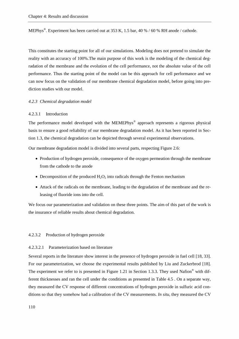
Chapter 4: Results and discussion
110
MEPhys®. Experiment has been carried out at 353 K, 1.5 bar, 40 % / 60 % RH anode / cathode.
This constitutes the starting point for all of our simulations. Modeling does not pretend to simulate the
reality with an accuracy of 100%.The main purpose of this work is the modeling of the chemical deg-
radation of the membrane and the evolution of the cell performance, not the absolute value of the cell
performance. Thus the starting point of the model can be this approach for cell performance and we
can now focus on the validation of our membrane chemical degradation model, before going into pre-
diction studies with our model.
4.2.3 Chemical degradation model
4.2.3.1 Introduction
The performance model developed with the MEMEPhys® approach represents a rigorous physical
basis to ensure a good reliability of our membrane degradation model. As it has been reported in Sec-
tion 1.3, the chemical degradation can be depicted through several experimental observations.
Our membrane degradation model is divided into several parts, respecting Figure 2.6:
Production of hydrogen peroxide, consequence of the oxygen permeation through the membrane
from the cathode to the anode
Decomposition of the produced H2O2 into radicals through the Fenton mechanism
Attack of the radicals on the membrane, leading to the degradation of the membrane and the re-
leasing of fluoride ions into the cell.
We focus our parameterization and validation on these three points. The aim of this part of the work is
the insurance of reliable results about chemical degradation.
4.2.3.2 Production of hydrogen peroxide
4.2.3.2.1 Parameterization based on literature
Several reports in the literature show interest in the presence of hydrogen peroxide in fuel cell [18, 33].
For our parameterization, we choose the experimental results published by Liu and Zuckerbrod [18].
The experiment we refer to is presented in Figure 1.21 in Section 1.3.3. They used Nafion® with dif-
ferent thicknesses and ran the cell under the conditions as presented in Table 4.5 . On a separate way,
they measured the CV response of different concentrations of hydrogen peroxide in sulfuric acid con-
ditions so that they somehow had a calibration of the CV measurements. In situ, they measured the CV

Chapter 4: Results and discussion
111
response of the cell and deduced the concentration of hydrogen peroxide produced in the cell. The
advantage of these measurements is that they have been done for several membrane thicknesses. Thus
after having parameterized our simulation for a given thickness, we can test it by varying the mem-
brane thickness and comparing the simulations with experiment results.
Parameters Value Unit
Current density OCV -
Temperature 60 °C
Pressure 1 Bar
Relative humidity anode 100 %
Relative humidity cathode 100 %
Membrane thickness variable µm
Equivalent weight 1200 g·eq–1
Table 4.5: Experimental parameters used by Liu and Zuckerbrod
4.2.3.2.2 Simulations parameters and assumptions
In Section 2.3.1, we proposed a mechanism describing the H2O2 production. For these reactions, we
need the activation energies, so that Equation 3.17 can be used. Ferreira de Morais, within Franco’s
group performed DFT calculations for the oxygen reduction on platinum surface and obtained a set of
activation energy values both for H2O2 production reaction [84]. The values of these activation ener-
gies are given in Table 4.6. However parameters for oxygen adsorption and desorption on the catalyst
surface (Reaction 3.6) were not known and parameters found in the literature did not seem to be de-
termined under conditions close to the environment we simulate and thus no good agreement was
obtained compared to our objectives. Thus we fitted these values, so that the produced amount of H2O2
calculated by the model fits with experimental results. With the genetic algorithm embedded in
Matlab, we could set as aim the quantity of hydrogen peroxide for a 30 µm membrane and get the
desired parameters.
As in our complete degradation model hydrogen peroxide is decomposed into radicals, we switched
off the further degradation steps in the membrane (H2O2 decomposition through Fenton’s reactions
and radical attack on the membrane), so we can follow the concentration of produced H2O2. Moreover,
considering that the production of hydrogen peroxide is a continuous phenomenon, one could expect
that over time the concentration will increase. As we do not know their experiment duration, we de-
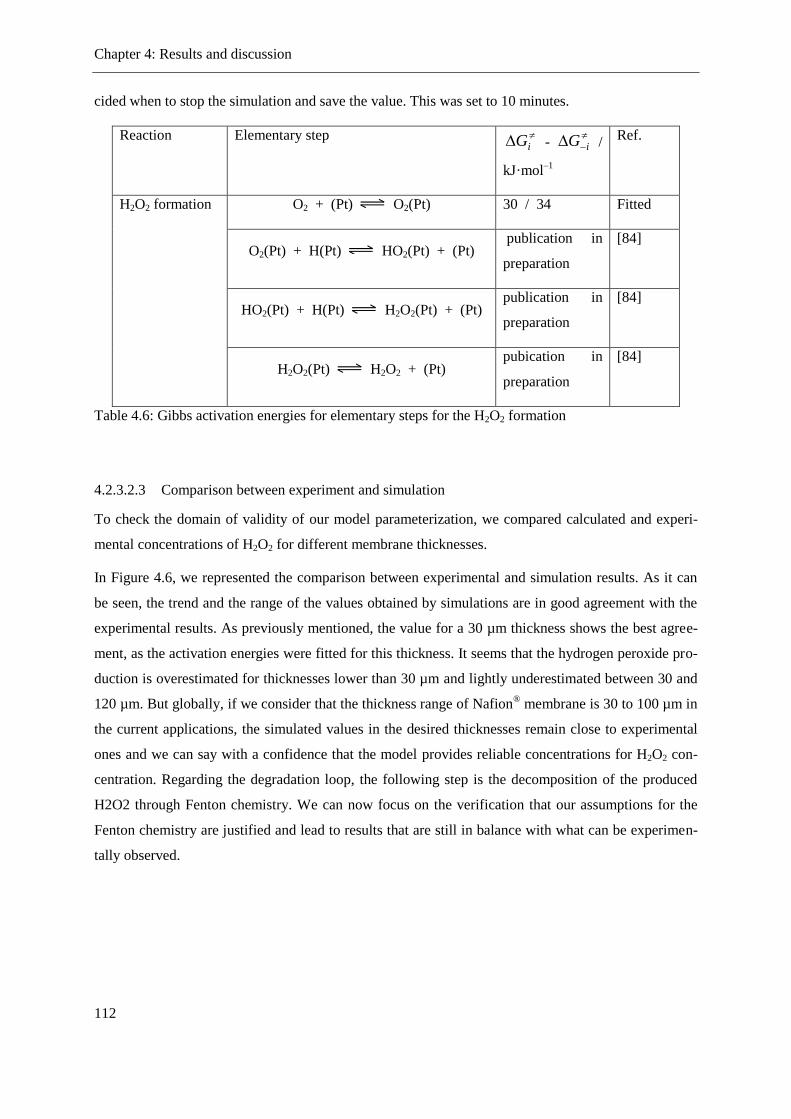
Chapter 4: Results and discussion
112
cided when to stop the simulation and save the value. This was set to 10 minutes.
Reaction Elementary step iG - iG /
kJ·mol–1
Ref.
H2O2 formation O2 + (Pt) O2(Pt) 30 / 34 Fitted
O2(Pt) + H(Pt) HO2(Pt) + (Pt) publication in
preparation
[84]
HO2(Pt) + H(Pt) H2O2(Pt) + (Pt) publication in
preparation
[84]
H2O2(Pt) H2O2 + (Pt) pubication in
preparation
[84]
Table 4.6: Gibbs activation energies for elementary steps for the H2O2 formation
4.2.3.2.3 Comparison between experiment and simulation
To check the domain of validity of our model parameterization, we compared calculated and experi-
mental concentrations of H2O2 for different membrane thicknesses.
In Figure 4.6, we represented the comparison between experimental and simulation results. As it can
be seen, the trend and the range of the values obtained by simulations are in good agreement with the
experimental results. As previously mentioned, the value for a 30 µm thickness shows the best agree-
ment, as the activation energies were fitted for this thickness. It seems that the hydrogen peroxide pro-
duction is overestimated for thicknesses lower than 30 µm and lightly underestimated between 30 and
120 µm. But globally, if we consider that the thickness range of Nafion® membrane is 30 to 100 µm in
the current applications, the simulated values in the desired thicknesses remain close to experimental
ones and we can say with a confidence that the model provides reliable concentrations for H2O2 con-
centration. Regarding the degradation loop, the following step is the decomposition of the produced
H2O2 through Fenton chemistry. We can now focus on the verification that our assumptions for the
Fenton chemistry are justified and lead to results that are still in balance with what can be experimen-
tally observed.

Chapter 4: Results and discussion
113
Figure 4.6: Comparison experiment / simulation for the hydrogen peroxide production
4.2.3.3 Fenton chemistry and production of radicals
4.2.3.3.1 Literature experiment
The decomposition of hydrogen peroxide through reaction with iron ions has already been widely
studied since the 1890s by Henry Fenton. It is a useful reaction for the oxidation of organic com-
pounds in water, as the produced radicals are highly oxidative species and can attack even the most
stabile pollutants in water [23, 24, 157].
But in a PEMFC, this reaction may be dramatic, as the presence of radicals in the system will lead to a
chemical attack on the membrane, degrading the cell integrity. However, even if we know that they are
present in the system, they are such reactive species that their lifetime lies of about 1 ns. Thus their
direct observation is really complex and needs specifically and complex experimental devices like
ESR or EPR. Some articles report the results of the application of such methods [28-30, 92]. We took
a closer look on the work by Aoki et al. [91]. They performed ESR measurements to quantify the
amount of radicals produced in the membrane after different treatments. The one of interest for us was
conducted on a membrane soaked in Fenton’s reagent for 5 minutes (see more precision in Table 4.7).
They found out that the quantity of produced radicals is independent of the nature of the membrane.
20 40 60 80 100 120 140
0.0
0.2
0.4
0.6
0.8
1.0
1.2
H2O
2 c
on
ce
ntr
atio
n
/ m
mo
l·m
3
Membrane thickness / µm
Experiment
Simulation
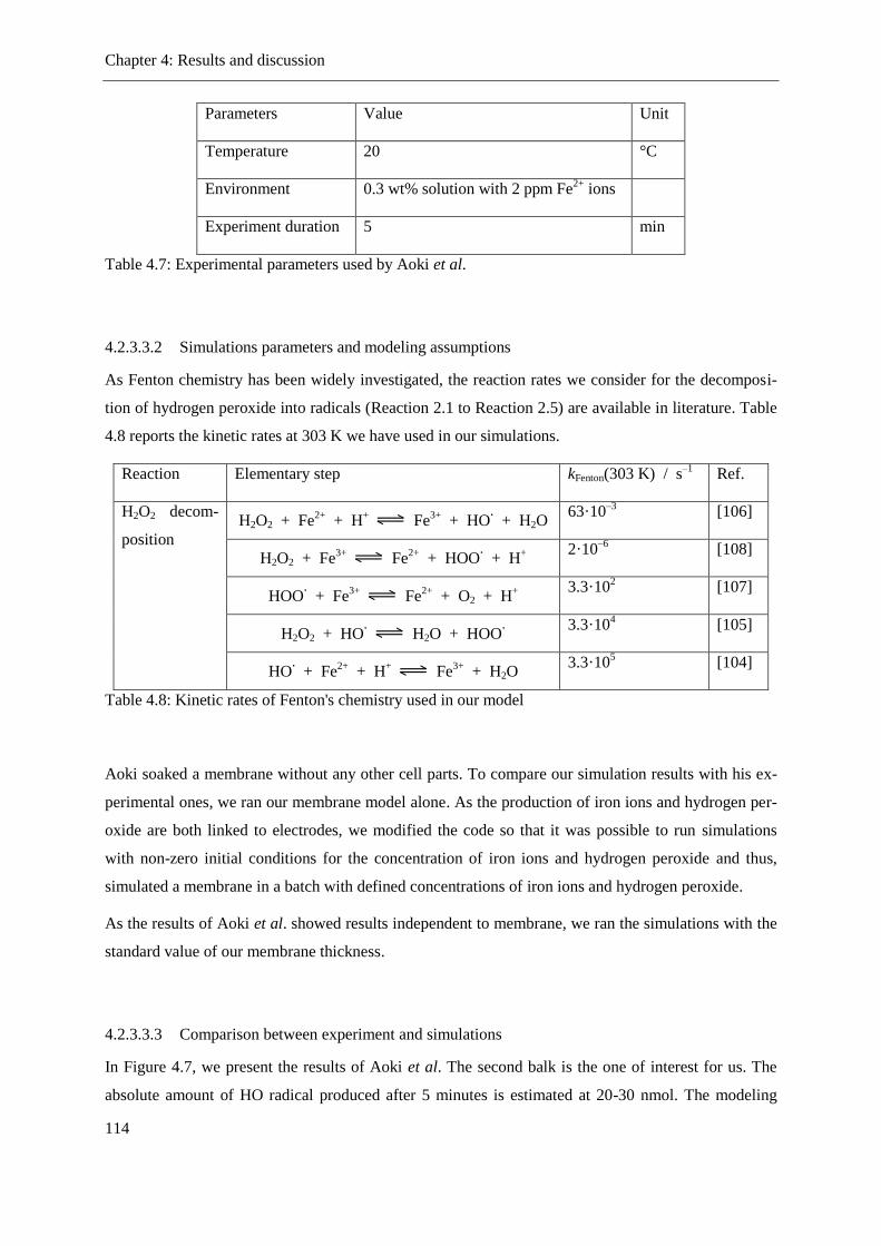
Chapter 4: Results and discussion
114
Parameters Value Unit
Temperature 20 °C
Environment 0.3 wt% solution with 2 ppm Fe2+
ions
Experiment duration 5 min
Table 4.7: Experimental parameters used by Aoki et al.
4.2.3.3.2 Simulations parameters and modeling assumptions
As Fenton chemistry has been widely investigated, the reaction rates we consider for the decomposi-
tion of hydrogen peroxide into radicals (Reaction 2.1 to Reaction 2.5) are available in literature. Table
4.8 reports the kinetic rates at 303 K we have used in our simulations.
Reaction Elementary step kFenton(303 K) / s–1
Ref.
H2O2 decom-
position
H2O2 + Fe2+
+ H+ Fe
3+ + HO
· + H2O
63·10–3
[106]
H2O2 + Fe3+
Fe2+
+ HOO· + H
+
2·10–6
[108]
HOO· + Fe
3+ Fe
2+ + O2 + H
+
3.3·102 [107]
H2O2 + HO· H2O + HOO
·
3.3·104 [105]
HO· + Fe
2+ + H
+ Fe
3+ + H2O
3.3·105 [104]
Table 4.8: Kinetic rates of Fenton's chemistry used in our model
Aoki soaked a membrane without any other cell parts. To compare our simulation results with his ex-
perimental ones, we ran our membrane model alone. As the production of iron ions and hydrogen per-
oxide are both linked to electrodes, we modified the code so that it was possible to run simulations
with non-zero initial conditions for the concentration of iron ions and hydrogen peroxide and thus,
simulated a membrane in a batch with defined concentrations of iron ions and hydrogen peroxide.
As the results of Aoki et al. showed results independent to membrane, we ran the simulations with the
standard value of our membrane thickness.
4.2.3.3.3 Comparison between experiment and simulations
In Figure 4.7, we present the results of Aoki et al. The second balk is the one of interest for us. The
absolute amount of HO radical produced after 5 minutes is estimated at 20-30 nmol. The modeling

Chapter 4: Results and discussion
115
results are shown in Figure 4.8. After 5 min, the simulation shows a very low HO radical concentra-
tion. Simultaneously, the concentration of HO2 radical increases up to 0.13 mmol·L–1
.
To compare with the results of Aoki, we convert them into an absolute amount of radical. Considering
our standard cell membrane with 25cm² geometric area and 60 µm thickness, this leads to an absolute
amount of 0.13·60·10–6
·25·10–4
= 19.50·10–9
mol = 19.50 nmol. This is a good agreement with Aoki’s
work. But it remains explaining why our HO2 radical concentration value and not our HO radical con-
centration is comparable to the work of Aoki et al.
They are using spin trap reagent (DMPO) in their experiment. This molecule reacts quickly with HO
radicals to form DMPO-OH adduct, thus the radicals do not have the possibility to evolve after reac-
tions of Table 4.8. In our case, the HO radicals are not trapped and can then be involved in other reac-
tions of the Fenton’s chemistry. More particularly in Reaction 2.4: HO radicals can react with a quite
high kinetic rate with H2O2 to form HO2 radicals. This explains why we compared the total amount of
radicals in our model with HO radical amount measured by Aoki.
Figure 4.7: Hydroxyl radical generated in membrane in different solutions [91]
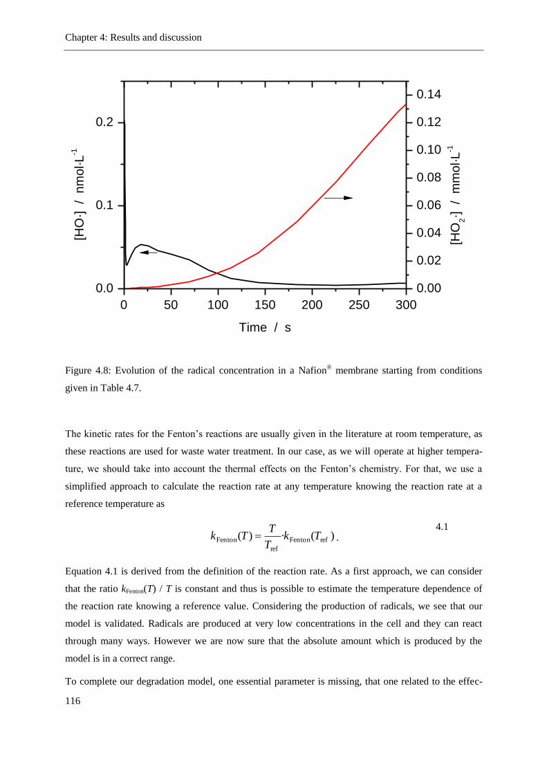
Chapter 4: Results and discussion
116
Figure 4.8: Evolution of the radical concentration in a Nafion® membrane starting from conditions
given in Table 4.7.
The kinetic rates for the Fenton’s reactions are usually given in the literature at room temperature, as
these reactions are used for waste water treatment. In our case, as we will operate at higher tempera-
ture, we should take into account the thermal effects on the Fenton’s chemistry. For that, we use a
simplified approach to calculate the reaction rate at any temperature knowing the reaction rate at a
reference temperature as
)(·)( refFenton
ref
Fenton TkT
TTk .
4.1
Equation 4.1 is derived from the definition of the reaction rate. As a first approach, we can consider
that the ratio kFenton(T) / T is constant and thus is possible to estimate the temperature dependence of
the reaction rate knowing a reference value. Considering the production of radicals, we see that our
model is validated. Radicals are produced at very low concentrations in the cell and they can react
through many ways. However we are now sure that the absolute amount which is produced by the
model is in a correct range.
To complete our degradation model, one essential parameter is missing, that one related to the effec-
0 50 100 150 200 250 300
0.0
0.1
0.2
Time / s
[HO
·]
/ n
mo
l·L
-1
0.00
0.02
0.04
0.06
0.08
0.10
0.12
0.14
[HO
2·]
/
mm
ol·L
-1

Chapter 4: Results and discussion
117
tive reaction of the membrane degradation.
4.2.3.4 Degradation of the membrane and releasing of fluoride ions
4.2.3.4.1 Experimental studies
For our parameterization, the experimental results we choose were published by Young et al. [16].
They measured over time the cumulative production of fluoride ions of a cell under accelerated test
conditions, as mentioned in Table 1.4. A summary of the experimental parameters are given in Table
4.9. During their experiment, they sometimes shut down the cell for running extra analysis. We re-
moved the part were the cell was not operating anymore and got a shorter experiment for our valida-
tion (the duration of the experiment was reduced from 450 h to about 290 h, as it can be seen in Figure
4.9). This was also used for our parameterization.
Parameters Value Unit
Current density OCV
Duration 450 (corrected 290) h
Pressure 2 bar
Temperature 90 °C
Membrane thickness 60 µm
Equivalent weight 1100 g·eq–1
Relative humidity 100 %
Pt load cathode 0.60 mg·cm–2
Pt load anode 0.30 mg·cm–2
Table 4.9: Experimental parameters used by Young et al. for the determination of cumulative fluoride
ions released under AST.
Last they plotted the cumulative release of fluoride ions, and our model computes instantaneous con-
centration. Thus we had to integrate our output signal to be able to compare experiment and modeling
results.
4.2.3.4.2 Simulations parameters and modeling assumptions

Chapter 4: Results and discussion
118
As assumed in Section 2.3.2, side chain degradation is supposed to drive the production kinetic of
fluoride ions, which is one of the most reported measurements in the literature to follow the chemical
degradation of the membrane. According to Equation 2.27, to get the concentration of fluoride ions,
we have to determine the evolution of the side chain concentration in the membrane. For that purpose,
one parameter is still needed, and this is the last one to determine to complete our degradation model.
The value of the kinetic constant of the side chain degradation we are searching is used in Equation
2.25. The rewriting of Equation 2.25 applied to side chains in the membrane leads to Equation 4.2,
chain sideHO·DEG
chain side ·· cckt
c
.
4.2
It has been shown that iron ions do have an important impact on the chemical degradation of the cell,
as they play a key role in the Fenton chemistry (Reaction 2.1 to Reaction 2.5 in Section 2.3.1). How-
ever it is difficult to predict if iron ions will be produced by the system, as the origin of the iron ions
remains a widely open question. Our assumption here is that the iron ions are produced by the bipolar
plate at the cathode, where the simultaneous presence of water, metallic iron and a high potential could
lead to the oxidation of iron metal into iron ions. To model that in a simple way, we add a constant
source term for iron ions at the cathode / membrane interface, noted
2FeS , which is then included in
the mass balance equation and thus taken into account in Equation 2.26. Its value will vary depending
on the system we will simulate: Low values for cell with low end-plate degradation (for example),
higher values for high end-plate degradation. For the purpose of our parameterization, we choose the
value of 3·10–5
mol·m–3
·s–1
.
4.2.3.4.3 Comparison between experiment and simulations
We had two unknown parameters and only one experiment result to exploit. By setting the production
term of iron ions at the cathode, we eliminate one parameter. To determine then the missing reaction
rate constant, we proceeded through the same analytical procedure as for the missing Gibbs activation
energies in Section 4.2.3.2. We used the optimization toolbox of Matlab, and set as end value the cu-
mulative fluoride amount measured by Young et al. at the end of their experiment (450 h real, 290 h if
we ignore the shutdown phase). Setting a fixed rate of production of iron ions at the cathode of 3·10–5
mol·m–3
·s–1
, the best compromise we found for the side chain scission reaction rate was 4.5 s–1
. This
value depends on the rate of iron production. If more information were provided concerning the pro-
duction of iron by the system, we may have parameterized our model on a more reliable way.
Young et al. carried out their experiment a high temperature (for a common Nafion® membrane), that
is to say 90 °C. As we simulate cases where the temperature is up to 30 °C lower as well, we have to
take into account the thermal effects for the chemical degradation. From the value of 4.5 s–1
we got
from the parameterization, we deduced an approximation of Gibbs activation energy for the degrada-
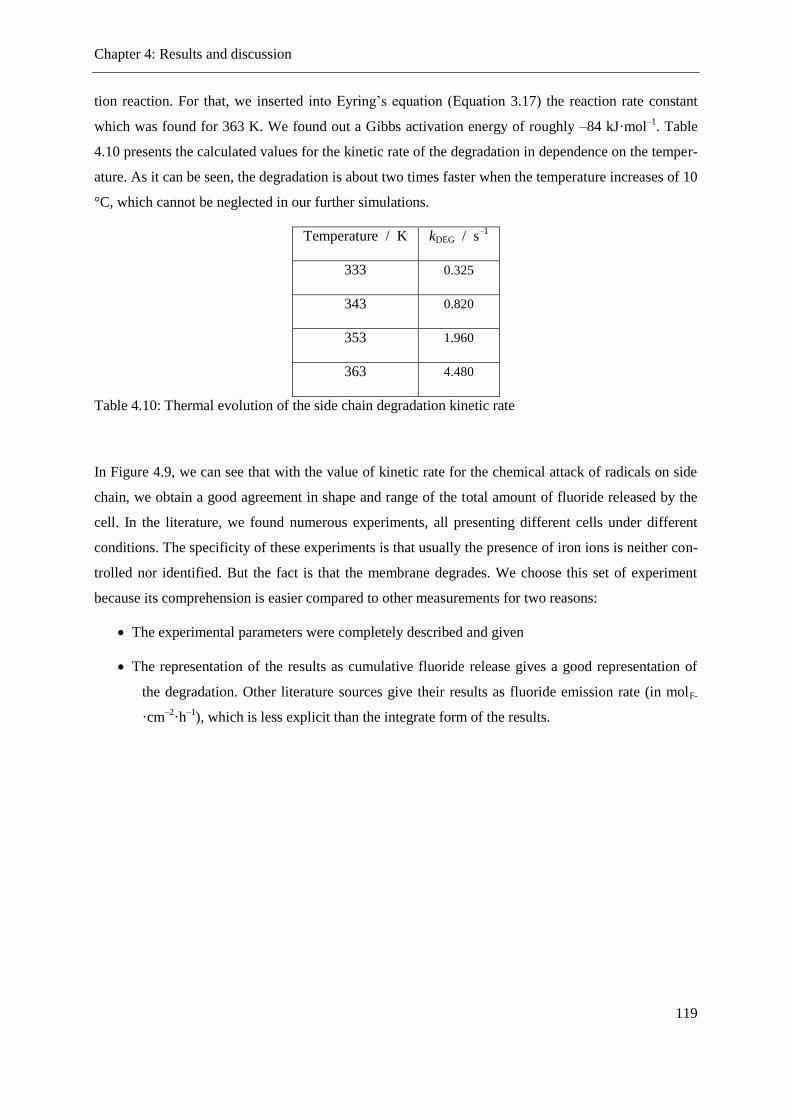
Chapter 4: Results and discussion
119
tion reaction. For that, we inserted into Eyring’s equation (Equation 3.17) the reaction rate constant
which was found for 363 K. We found out a Gibbs activation energy of roughly –84 kJ·mol–1
. Table
4.10 presents the calculated values for the kinetic rate of the degradation in dependence on the temper-
ature. As it can be seen, the degradation is about two times faster when the temperature increases of 10
°C, which cannot be neglected in our further simulations.
Temperature / K kDEG / s–1
333 0.325
343 0.820
353 1.960
363 4.480
Table 4.10: Thermal evolution of the side chain degradation kinetic rate
In Figure 4.9, we can see that with the value of kinetic rate for the chemical attack of radicals on side
chain, we obtain a good agreement in shape and range of the total amount of fluoride released by the
cell. In the literature, we found numerous experiments, all presenting different cells under different
conditions. The specificity of these experiments is that usually the presence of iron ions is neither con-
trolled nor identified. But the fact is that the membrane degrades. We choose this set of experiment
because its comprehension is easier compared to other measurements for two reasons:
The experimental parameters were completely described and given
The representation of the results as cumulative fluoride release gives a good representation of
the degradation. Other literature sources give their results as fluoride emission rate (in molF-
·cm–2
·h–1
), which is less explicit than the integrate form of the results.

Chapter 4: Results and discussion
120
Figure 4.9: Comparison experiment / simulation for the cumulative production of fluoride ion
We are now sure that the use of our model would not give results that are unrealistic. We aim then our
work on the prediction of trends with the help of our model.
The results in the next part do not pretend to give accurate results of what would be experimentally
observed, but rather pretend to give trends on cells behaviors under different architectures, stresses and
experimental conditions, that could constitute some guidelines for engineering enhancement of the
PEMFC durability.
4.2.4 Influence of experimental conditions on chemical degradation
An increase of the temperature translates into a higher degradation rate of the membrane. As a first
approximation, we can say that an increase of 10 K of the temperature will double the effect of the
cumulative fluoride production, which refers to the thermal evolution of the side chain degradation
kinetic rate (Table 4.10). This confirms the importance of thermal effects on the different kinetic rates
of the model. This result is in agreement with experimental work which can be found in the literature.
Kodama et al. presented results were they degraded ex-situ Nafion® membranes in hydrogen peroxide
[158, 159]. Even if the range of their results cannot be compared with our modeling results (we simu-
lated the operation of a complete fuel cell), the trend is in agreement with the evolution of the degrada-
tion with temperature what we get from the simulations. If we compare the evolution between 60 °C
0 50 100 150 200 250 300
0
1
2
3
4
5
6
Cu
mu
lativ
e F
- re
lea
se
/ µ
mo
l·cm
-2
Time / h
Experiment
Simulation
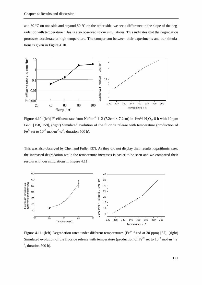
Chapter 4: Results and discussion
121
and 80 °C on one side and beyond 80 °C on the other side, we see a difference in the slope of the deg-
radation with temperature. This is also observed in our simulations. This indicates that the degradation
processes accelerate at high temperature. The comparison between their experiments and our simula-
tions is given in Figure 4.10
Figure 4.10: (left) F- effluent rate from Nafion
® 112 (7.2cm × 7.2cm) in 1wt% H2O2, 8 h with 10ppm
Fe2+ [158, 159], (right) Simulated evolution of the fluoride release with temperature (production of
Fe2+
set to 10–3
mol·m–3
·s–1
, duration 500 h).
This was also observed by Chen and Fuller [37]. As they did not display their results logarithmic axes,
the increased degradation while the temperature increases is easier to be seen and we compared their
results with our simulations in Figure 4.11.
Figure 4.11: (left) Degradation rates under different temperatures (Fe2+
fixed at 30 ppm) [37], (right)
Simulated evolution of the fluoride release with temperature (production of Fe2+
set to 10–3
mol·m–3
·s–
1, duration 500 h).

Chapter 4: Results and discussion
122
4.2.5 Validity of the model
We propose in this work prediction tool for evolution of PEMFC performance when chemical degra-
dation is taken into account in the cell. This phenomenon is very difficult to treat, as its occurrence is
barely predictable because of the need of iron ions in the system. Even if the chemical degradation of
the membrane is an actor of cell failure, it is not the major contributor for cell failure [70]. Thus it is
more difficult to give rise to its impact on the degradation of cell performance. However, through the
simulated fluoride emission, it is possible to see how severely the membrane is attacked.
Like every modeling work, it relies on assumptions and approximations. The purpose of this Section is
to analyze the reliability of the results we obtained in this chapter.
The model we developed in this thesis is to our knowledge the first one in the literature which explicit-
ly correlates the chemical degradation of the cell and their impact on the cell properties and perfor-
mances. As the model is complex and multiscale, it requires lot of parameters which are not necessari-
ly available in the literature. To solve this problem, comparisons with similar system allow knowing
the range of missing parameters, for example the diffusion coefficients of species in PFSA membrane.
The core of the performance model, the electrodes, are complex and relies as well on the knowledge of
kinetics parameters which are the results of atomistic simulations, and thus, if the data are not availa-
ble, fitting remains the only way to complete the electrodes models. In an updated model, thanks the
work of Ferreira de Morais et al. the ORR mechanism is better known [84, 153].
The last point which should be noticed on our model is the quantification of the influence of iron ions.
To reproduce experimental results, we had to simulate cells whose iron ions production is unrealistic.
We assume the cause is our assumption on the Fenton chemistry. We assume only a limited number of
possibilities for the iron to react. In a real system, possibilities are higher, as the iron ions could react
in a more complex way, as displayed in Appendix B.
But our model returns results which are consistent with experimental observations made. We validated
the model by reducing as much as possible the number of parameters to fit fitting lot of parameters and
rely on data available in the literature. The degradation model, even if it has been simplified, provides
good agreement with experimental results. As our modeling work is flexible, any improvement can
then be implemented to make the simulations more accurate.
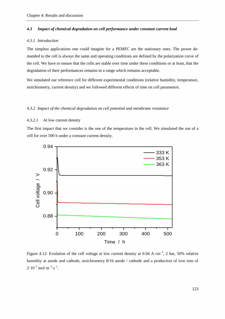
Chapter 4: Results and discussion
123
4.3 Impact of chemical degradation on cell performance under constant current load
4.3.1 Introduction
The simplest applications one could imagine for a PEMFC are the stationary ones. The power de-
manded to the cell is always the same and operating conditions are defined by the polarization curve of
the cell. We have to ensure that the cells are stable over time under these conditions or at least, that the
degradation of their performances remains in a range which remains acceptable.
We simulated our reference cell for different experimental conditions (relative humidity, temperature,
stoichiometry, current density) and we followed different effects of time on cell parameters.
4.3.2 Impact of the chemical degradation on cell potential and membrane resistance
4.3.2.1 At low current density
The first impact that we consider is the one of the temperature in the cell. We simulated the run of a
cell for over 500 h under a constant current density.
Figure 4.12: Evolution of the cell voltage at low current density at 0.04 A·cm–2
, 2 bar, 50% relative
humidity at anode and cathode, stoichiometry 8/16 anode / cathode and a production of iron ions of
2·10–5
mol·m–3
·s–1
.
0 100 200 300 400 500
0.88
0.90
0.92
0.94
333 K
353 K
363 K
Cell
volta
ge
/
V
Time / h

Chapter 4: Results and discussion
124
Figure 4.12 shows the evolution of the cell voltage at a given relative humidity. We observe that the
cell voltage decreases with increasing temperature. This is in contradiction with the laws of kinetics,
saying that with increasing temperature, the reaction rate of HOR and ORR would be faster. Moreover
the thermal effects are taken into account as well in our degradation model. So how could one explain
this divergence from the theory?
At every temperature, we set the relative humidity constant in both electrodes. The relative humidity is
defined as the ratio of the partial pressure of water vapor to the saturated water vapor pressure. In Fig-
ure 4.13, we represented the evolution of the water saturated vapor pressure with temperature. As it
can be seen, there is a strong dependence of temperature. Thus, considering the same relative humidity
at 333 K and 363 K and the strong variation of saturated vapor pressure, the partial pressure of water
vapor will increase with increasing temperature. Our simulation are isobar, the total pressure is con-
stant at each side. The global pressure is defined as the sum of the oxygen partial pressure and the
water partial pressure at the cathode side. If the water partial pressure increases with temperature, the
partial pressure of oxygen will decrease to balance this effect and keep the pressure constant. In Figure
4.14, the profiles of dissolved oxygen in the membrane are represented. The value at the cathode side
is directly linked to the partial pressure of oxygen through Henry’s law (Equation 2.21).
Figure 4.13: Evolution of the water saturated vapor pressure with temperature from 0 °C to 100 °C.
280 300 320 340 360
0
20000
40000
60000
80000
100000
Wa
ter
sa
tura
ted
va
po
r p
ressu
re
/ P
a
Temperature / K

Chapter 4: Results and discussion
125
But if we compare Figure 1.15 and Figure 4.12, we see that our modeling predictions show no signifi-
cant changes in the cell potential at the low current density over time, whereas the experimental results
show on the contrary a diminution of the cell potential. Our degradation model takes into account the
evolution of the cell resistance over time, and its changes are responsible for the performance degrada-
tion of the cell. As this effect is purely an ohmic one, it is obvious that when the current density ap-
plied is set close to 0, changes in the ohmic contribution of the potential are negligible. Thus the cause
of potential degradation under low current density conditions cannot be attributed to the chemical deg-
radation of the membrane.
A possible explanation for this observation could be the simultaneous presence of oxygen (because of
its permeation through the membrane) and hydrogen at the anode side. This would imply the for-
mation of a mixed potential which negatively impact on the cell potential. As one of the consequences
of the degradation is a loss of matter and thus an increase of transport phenomena, the increased oxy-
gen cross-over would then explain the degradation of the cell potential at low current density. This
remains a hypothesis, as the model does not currently take this into account, we could not predict it.
Figure 4.14: Dissolved oxygen concentration profile at 0.04 A·cm–2
, 2 bar, 50% relative humidity at
anode and cathode, stoichiometry 8/16 anode / cathode and a production of iron ions of 2·10–5
mol·m–
3·s
–1.
0.0 0.2 0.4 0.6 0.8 1.0
0
1
2
3
Anode
333 K
353 K
363 K
[Odis
solv
ed
2]m
ol·
m-3
Position in the membrane / -
Cath
ode

Chapter 4: Results and discussion
126
In our simulations, we observe under low current conditions a small decrease of the cell voltage
(Figure 4.12). This is due to the increase in the ohmic losses. But as the absolute current applied is 1
A, this potential decrease is not significant. As previously mentioned, the mixed potential allows ex-
plaining the potential decrease at OCV, as no oxygen reacts and the permeation of oxygen to the anode
is enhanced. With increasing current density, this mixed potential decreases, as the permeation is not
so large and oxygen is consumed, but the ohmic losses increases, as the current is higher.
Because of the different sources of cell potential degradation depending on current density, we do not
choose potential degradation as parameter to monitor the chemical degradation of the membrane but
the evolution of the membrane resistance.
In Figure 4.15 (a), we plot the evolution of the membrane resistance with time for our low current
density experiment. Two different phases are identified. The first fast increasing of the membrane
resistance is due to the driving of the system to stable conditions (this is usually due to approximation
in the choice of start conditions).
During the second phase (Figure 4.15 (b)), the membrane resistance increase is weaker. As mentioned
in Section 4.1, a small amount of water is produced in our low current conditions and depending on
the temperature; the humidification of the membrane will be different depending on the temperature.
The water profile in the membrane is shown in Figure 4.16. We see strong differences in the humidifi-
cation, having an impact on the value of the membrane resistance.

Chapter 4: Results and discussion
127
Figure 4.15: Evolution of the membrane resistance at 0.04 A·cm–2
, 2 bar, 50% relative humidity at
anode and cathode, stoichiometry 8/16 anode / cathode and a production of iron ions of 2·10–5
mol·m–
3·s
–1 (a) Complete signal (b) Zoom in the dashed area.
0 100 200 300 400 500
10
12
14
16(b)
Me
mb
ran
e r
esis
tan
ce
/ m
Time / h
0 100 200 300 400 500
2468
1012141618
333 K
353 K
363 K
Me
mb
ran
e r
esis
tan
ce
/ m
(a)
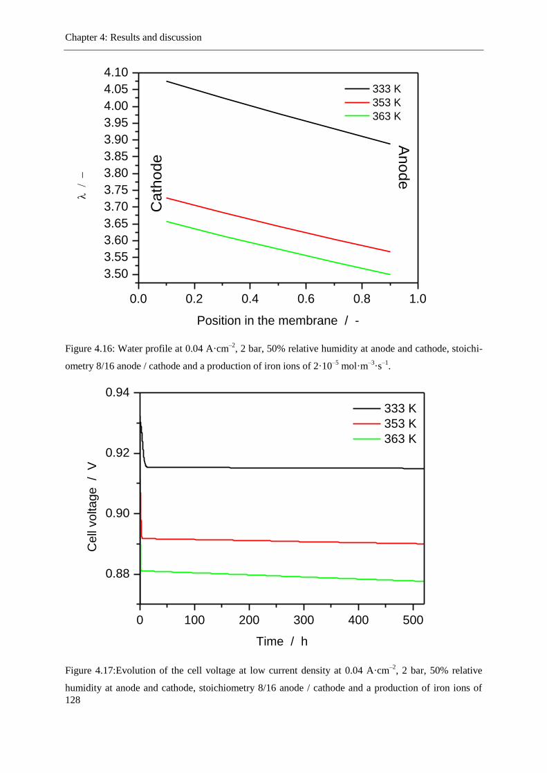
Chapter 4: Results and discussion
128
Figure 4.16: Water profile at 0.04 A·cm–2
, 2 bar, 50% relative humidity at anode and cathode, stoichi-
ometry 8/16 anode / cathode and a production of iron ions of 2·10–5
mol·m–3
·s–1
.
Figure 4.17:Evolution of the cell voltage at low current density at 0.04 A·cm–2
, 2 bar, 50% relative
humidity at anode and cathode, stoichiometry 8/16 anode / cathode and a production of iron ions of
0.0 0.2 0.4 0.6 0.8 1.0
3.50
3.55
3.60
3.65
3.70
3.75
3.80
3.85
3.90
3.95
4.00
4.05
4.10
Anode
333 K
353 K
363 K
Position in the membrane / -
Ca
tho
de
0 100 200 300 400 500
0.88
0.90
0.92
0.94
333 K
353 K
363 K
Cell
volta
ge
/
V
Time / h
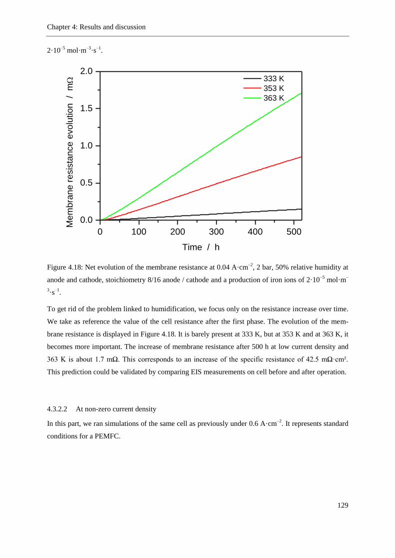
Chapter 4: Results and discussion
129
2·10–5
mol·m–3
·s–1
.
Figure 4.18: Net evolution of the membrane resistance at 0.04 A·cm–2
, 2 bar, 50% relative humidity at
anode and cathode, stoichiometry 8/16 anode / cathode and a production of iron ions of 2·10–5
mol·m–
3·s
–1.
To get rid of the problem linked to humidification, we focus only on the resistance increase over time.
We take as reference the value of the cell resistance after the first phase. The evolution of the mem-
brane resistance is displayed in Figure 4.18. It is barely present at 333 K, but at 353 K and at 363 K, it
becomes more important. The increase of membrane resistance after 500 h at low current density and
363 K is about 1.7 mΩ. This corresponds to an increase of the specific resistance of 42.5 mΩ·cm².
This prediction could be validated by comparing EIS measurements on cell before and after operation.
4.3.2.2 At non-zero current density
In this part, we ran simulations of the same cell as previously under 0.6 A·cm–2
. It represents standard
conditions for a PEMFC.
0 100 200 300 400 500
0.0
0.5
1.0
1.5
2.0 333 K
353 K
363 K
M
em
bra
ne r
esis
tance
evo
lution
/
m
Time / h
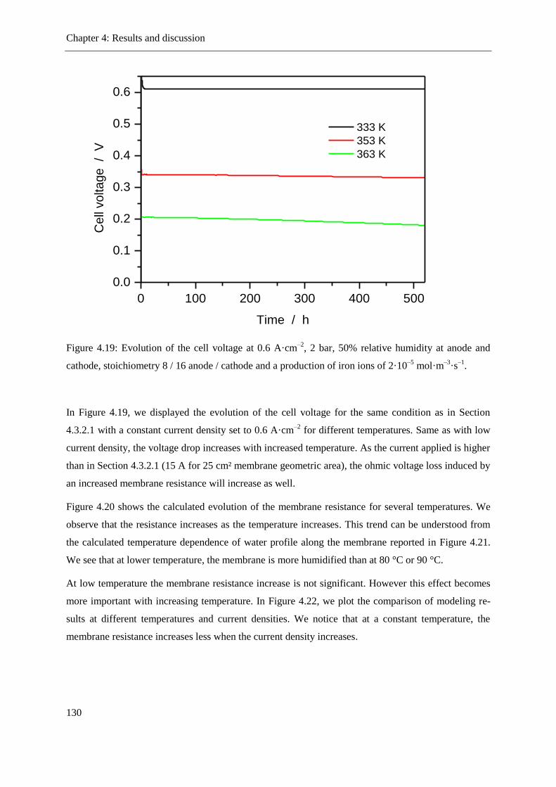
Chapter 4: Results and discussion
130
Figure 4.19: Evolution of the cell voltage at 0.6 A·cm–2
, 2 bar, 50% relative humidity at anode and
cathode, stoichiometry 8 / 16 anode / cathode and a production of iron ions of 2·10–5
mol·m–3
·s–1
.
In Figure 4.19, we displayed the evolution of the cell voltage for the same condition as in Section
4.3.2.1 with a constant current density set to 0.6 A·cm–2
for different temperatures. Same as with low
current density, the voltage drop increases with increased temperature. As the current applied is higher
than in Section 4.3.2.1 (15 A for 25 cm² membrane geometric area), the ohmic voltage loss induced by
an increased membrane resistance will increase as well.
Figure 4.20 shows the calculated evolution of the membrane resistance for several temperatures. We
observe that the resistance increases as the temperature increases. This trend can be understood from
the calculated temperature dependence of water profile along the membrane reported in Figure 4.21.
We see that at lower temperature, the membrane is more humidified than at 80 °C or 90 °C.
At low temperature the membrane resistance increase is not significant. However this effect becomes
more important with increasing temperature. In Figure 4.22, we plot the comparison of modeling re-
sults at different temperatures and current densities. We notice that at a constant temperature, the
membrane resistance increases less when the current density increases.
0 100 200 300 400 500
0.0
0.1
0.2
0.3
0.4
0.5
0.6
333 K
353 K
363 K
Ce
ll vo
lta
ge
/
V
Time / h

Chapter 4: Results and discussion
131
Figure 4.20: Evolution of membrane resistance at 0.6 A·cm–2
, 2 bar, 50% relative humidity at anode
and cathode, stoichiometry 8 / 16 anode / cathode and a production of iron ions of 2·10–5
mol·m–3
·s–1
.
Figure 4.21: Water content profile in the membrane at 0.6 A·cm–2
, 2 bar, 50% relative humidity at
0 100 200 300 400 500
4
6
14
16
18
20
333 K
353 K
363 K
Mem
bra
ne r
esis
tance
/
m
Time / h
0.0 0.2 0.4 0.6 0.8 1.0
2
4
6
8
Anode
333 K
353 K
363 K
Position in the membrane / -
Cath
ode
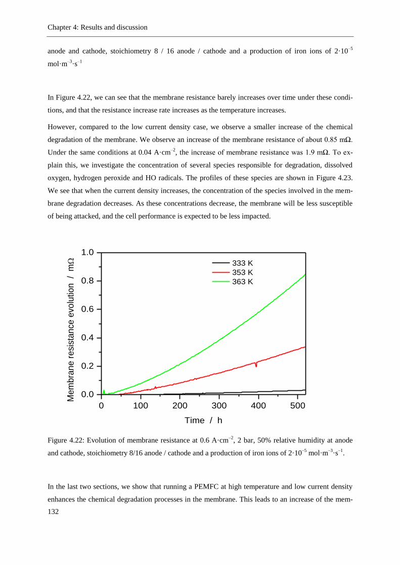
Chapter 4: Results and discussion
132
anode and cathode, stoichiometry 8 / 16 anode / cathode and a production of iron ions of 2·10–5
mol·m–3
·s–1
In Figure 4.22, we can see that the membrane resistance barely increases over time under these condi-
tions, and that the resistance increase rate increases as the temperature increases.
However, compared to the low current density case, we observe a smaller increase of the chemical
degradation of the membrane. We observe an increase of the membrane resistance of about 0.85 mΩ.
Under the same conditions at 0.04 A·cm–2
, the increase of membrane resistance was 1.9 mΩ. To ex-
plain this, we investigate the concentration of several species responsible for degradation, dissolved
oxygen, hydrogen peroxide and HO radicals. The profiles of these species are shown in Figure 4.23.
We see that when the current density increases, the concentration of the species involved in the mem-
brane degradation decreases. As these concentrations decrease, the membrane will be less susceptible
of being attacked, and the cell performance is expected to be less impacted.
Figure 4.22: Evolution of membrane resistance at 0.6 A·cm–2
, 2 bar, 50% relative humidity at anode
and cathode, stoichiometry 8/16 anode / cathode and a production of iron ions of 2·10–5
mol·m–3
·s–1
.
In the last two sections, we show that running a PEMFC at high temperature and low current density
enhances the chemical degradation processes in the membrane. This leads to an increase of the mem-
0 100 200 300 400 500
0.0
0.2
0.4
0.6
0.8
1.0
333 K
353 K
363 K
Mem
bra
ne r
esis
tance
evo
lution
/
m
Time / h

Chapter 4: Results and discussion
133
brane resistance. This resistance increase induces a decrease of the cell potential which can be signifi-
cant if the current applied is high enough. However, membrane resistance is also influenced by the
water content in the membrane. Thus, to uncorrelate the humidification effect from the degradation
effect on the membrane resistance, we focus the next section of our work on a parameter representa-
tive of the degradation: the cumulative fluoride ions release.
Figure 4.23: Concentration profiles of different species at 0.6 A·cm–2
, 2 bar, 50% relative humidity at
anode and cathode, stoichiometry 8/16 anode / cathode and a production of iron ions of 2·10–5
mol·m–
3·s
–1
4.3.2.3 Impact of degradation on chemical composition
As mentioned in Section 4.1, the stoichiometry of the reactants has a certain impact on the humidifica-
tion of the membrane.
In Figure 4.24, we compare the calculated degradation of a cell whose reactants are fed at low and
high stoichiometry and under OCV conditions. It appears that lower stoichiometry enhances the deg-
radation of the cell. This is the consequence of humidification differences in the membrane: as case 2 /
4 is higher humidified as case 8 / 16, this may mean that if the relative humidity increases, the mem-
brane would be more degraded; this point will be further inquired in the next paragraphs.
0.0 0.2 0.4 0.6 0.8 1.0
0.0
0.5
1.0
1.5
2.0
[O2] / m
ol·
m-3
Position in the membrane / -
0.0 0.2 0.4 0.6 0.8 1.0
2
4
6
0.04 A·cm-2
0.6 A·cm-2
[HO
·] / n
mo
l·m
-3
Position in the membrane / -
0.0 0.2 0.4 0.6 0.8 1.0
0.020
0.025
0.030
0.035
0.040
[H2O
2] / m
ol·
m-3
Position in the membrane / -

Chapter 4: Results and discussion
134
Figure 4.24: Cumulative fluoride ions released by the cell at 4·10–2
A·cm–2
and different stoichiome-
try.
In Figure 4.25, we displayed the impact of the relative humidity on the chemical degradation of the
cell. We see that the membrane degrades more at higher relative humidity. The temporal evolution of
the fluoride is driven by Equation 4.2. As the kinetic rate is only temperature dependent, the source of
the differences is assumed to be the produced radical concentration. Thus we need a closer look on the
evolution of different concentrations in the membrane with the humidity.
0 100 200 300 400 500
0
2
4
6
8
10
12
14
16 333 K
353 K
363 K
Solid: 8 / 16
Dash : 2 / 4
Cu
mu
lative
F- r
ele
ase
/
µm
ol·
cm
-2
Time / h

Chapter 4: Results and discussion
135
Figure 4.25: Evolution of the degradation with relative humidity at 0.04 A·cm–2
, 2 bar, stoichiometry
2/4 anode / cathode and a production of iron ions of 10–3
mol·m–3
·s–1
.
In Figure 4.26, we displayed the profiles after 500 h for dissolved oxygen and hydrogen peroxide in
the membrane. As the oxygen comes into the membrane at the cathode side, it is normal that the con-
centration of oxygen is much higher at the cathode side. We see that the concentration of oxygen de-
creases with increasing humidity. This behavior is explained by the fact that at constant pressure, if we
increase the relative humidity (i.e. ratio of water in the gas), the corresponding ratio (i.e. partial pres-
sure) of oxygen will decrease. According to Henry’s law (Equation 2.21), it is then normal that the
concentration of dissolved oxygen decreases. But the range of the concentration remains close of each
other, which can then not alone explain the dependence of degradation on relative humidity.
However if we observe the evolution of the concentration of H2O2, we see that higher relative humidi-
ty greatly enhances the formation of H2O2. Thus more radicals will be produced and the membrane
will be more subject of being degraded. Experimental works reports in the literature provide contradic-
tory observations. Chen and Fuller showed that with increasing relative humidity, the concentration of
H2O2 will increase [36]. However in another publication they present another trend where the concen-
tration of H2O2 decreases with increasing relative humidity, implying a lower fluoride production [34].
Thus it is difficult to conclude anything about the coherence of the trend we simulate. If we yet refer to
0 200 400
0
10
20
30
40
50 50 %
70 %
90 %
Cu
mu
lative
F- r
ele
ase
/
µm
ol·
cm
-2
Time / h

Chapter 4: Results and discussion
136
the publications using an accelerated stress test, we may assume that high relative humidity enhances
the chemical degradation of the membrane [160].
Figure 4.26: Concentration profile of (a) O2 and (b) H2O2 in the membrane for different relative hu-
midity after 500 h at 0.04 A·cm–2
, 2 bar, stoichiometry 2/4 anode / cathode and a production of iron
ions of 10–3
mol·m–3
·s–1
.
Thus we performed the same simulations with a current density which is often taken as a operating
condition for PEMFC, 0.6 A·cm–2
.
As explained in Section 4.3.2.2, running a PEMFC at low current density will degrade it faster than at
high current density. But as the membrane resistance increase can, generally speaking, be an effect of
the water content as well, we have to compare the cumulative fluoride emissions for different cases.
Figure 4.27 shows the calculated concentrations of F- as function of the current density and the tem-
perature.
0.0 0.2 0.4 0.6 0.8 1.0
0.0
0.1
0.2
0.3
An
od
eA
no
de
Ca
tho
de
Ca
tho
de
(b)
[H2O
2]
/
mo
l·m
-3
Position in the membrane / -
0.0 0.2 0.4 0.6 0.8 1.0
0.0
0.5
1.0
1.5
2.0 50 %
70 %
90 %
[O2]
/
mo
l·m
-3
(a)
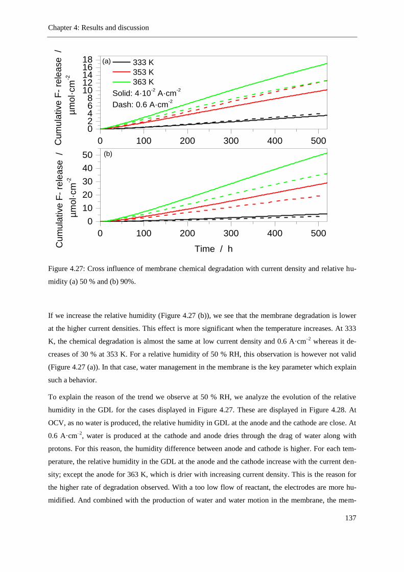
Chapter 4: Results and discussion
137
Figure 4.27: Cross influence of membrane chemical degradation with current density and relative hu-
midity (a) 50 % and (b) 90%.
If we increase the relative humidity (Figure 4.27 (b)), we see that the membrane degradation is lower
at the higher current densities. This effect is more significant when the temperature increases. At 333
K, the chemical degradation is almost the same at low current density and 0.6 A·cm–2
whereas it de-
creases of 30 % at 353 K. For a relative humidity of 50 % RH, this observation is however not valid
(Figure 4.27 (a)). In that case, water management in the membrane is the key parameter which explain
such a behavior.
To explain the reason of the trend we observe at 50 % RH, we analyze the evolution of the relative
humidity in the GDL for the cases displayed in Figure 4.27. These are displayed in Figure 4.28. At
OCV, as no water is produced, the relative humidity in GDL at the anode and the cathode are close. At
0.6 A·cm–2
, water is produced at the cathode and anode dries through the drag of water along with
protons. For this reason, the humidity difference between anode and cathode is higher. For each tem-
perature, the relative humidity in the GDL at the anode and the cathode increase with the current den-
sity; except the anode for 363 K, which is drier with increasing current density. This is the reason for
the higher rate of degradation observed. With a too low flow of reactant, the electrodes are more hu-
midified. And combined with the production of water and water motion in the membrane, the mem-
0 100 200 300 400 500
0
10
20
30
40
50 (b)
Cum
ula
tive F
- re
lea
se
/
µm
ol·
cm
-2
Time / h
0 100 200 300 400 500
02468
1012141618 333 K
353 K
363 K
Solid: 4·10-2 A·cm
-2
Dash: 0.6 A·cm-2
Cum
ula
tive F
- re
lea
se
/
µm
ol·
cm
-2(a)
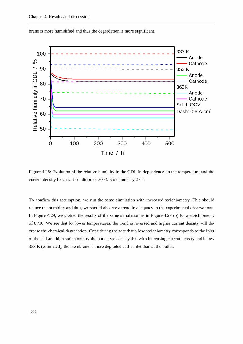
Chapter 4: Results and discussion
138
brane is more humidified and thus the degradation is more significant.
Figure 4.28: Evolution of the relative humidity in the GDL in dependence on the temperature and the
current density for a start condition of 50 %, stoichiometry 2 / 4.
To confirm this assumption, we run the same simulation with increased stoichiometry. This should
reduce the humidity and thus, we should observe a trend in adequacy to the experimental observations.
In Figure 4.29, we plotted the results of the same simulation as in Figure 4.27 (b) for a stoichiometry
of 8 /16. We see that for lower temperatures, the trend is reversed and higher current density will de-
crease the chemical degradation. Considering the fact that a low stoichiometry corresponds to the inlet
of the cell and high stoichiometry the outlet, we can say that with increasing current density and below
353 K (estimated), the membrane is more degraded at the inlet than at the outlet.
0 100 200 300 400 500
50
60
70
80
90
100 333 K
Anode
Cathode
353 K
Anode
Cathode
363K
Anode
Cathode
Solid: OCV
Dash: 0.6 A·cm-2
R
ela
tive
hu
mid
ity in
GD
L
/ %
Time / h
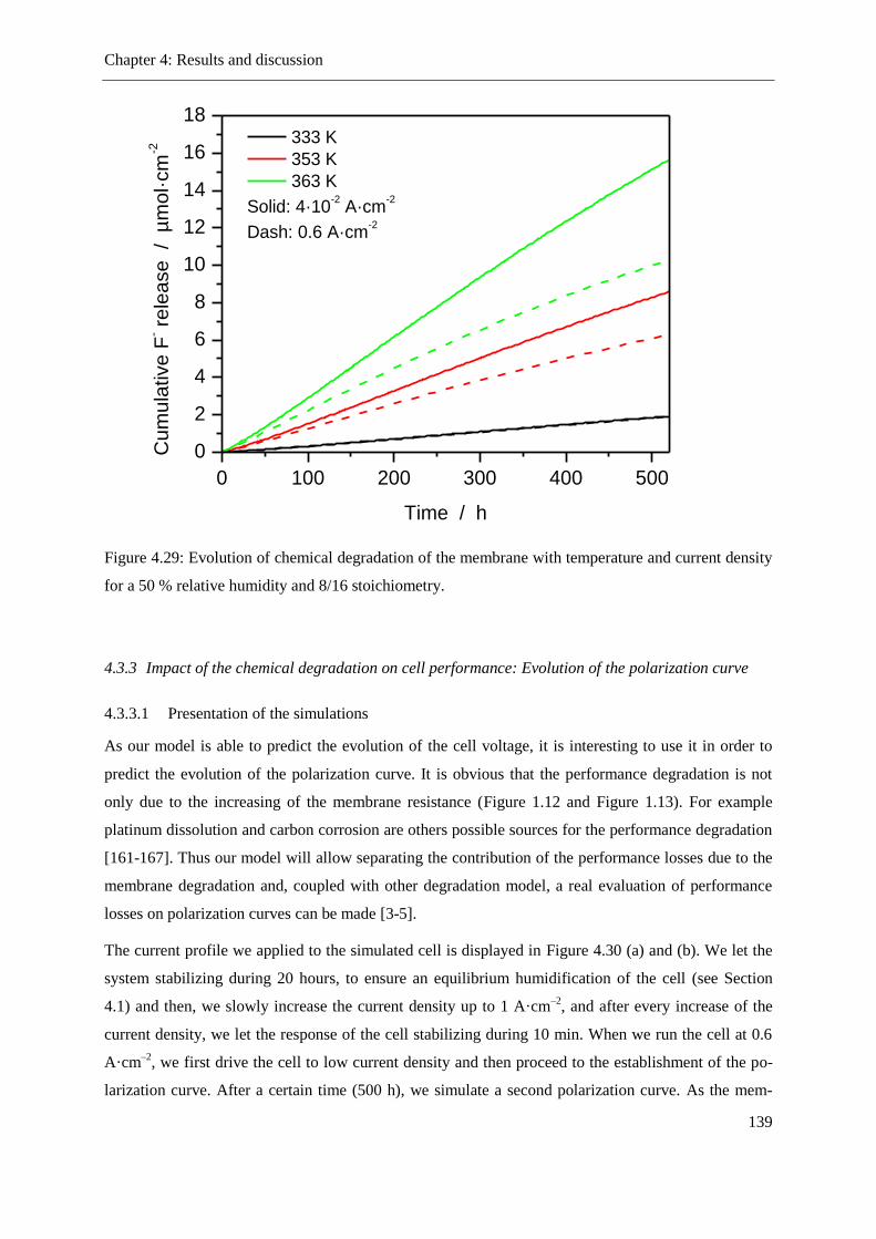
Chapter 4: Results and discussion
139
Figure 4.29: Evolution of chemical degradation of the membrane with temperature and current density
for a 50 % relative humidity and 8/16 stoichiometry.
4.3.3 Impact of the chemical degradation on cell performance: Evolution of the polarization curve
4.3.3.1 Presentation of the simulations
As our model is able to predict the evolution of the cell voltage, it is interesting to use it in order to
predict the evolution of the polarization curve. It is obvious that the performance degradation is not
only due to the increasing of the membrane resistance (Figure 1.12 and Figure 1.13). For example
platinum dissolution and carbon corrosion are others possible sources for the performance degradation
[161-167]. Thus our model will allow separating the contribution of the performance losses due to the
membrane degradation and, coupled with other degradation model, a real evaluation of performance
losses on polarization curves can be made [3-5].
The current profile we applied to the simulated cell is displayed in Figure 4.30 (a) and (b). We let the
system stabilizing during 20 hours, to ensure an equilibrium humidification of the cell (see Section
4.1) and then, we slowly increase the current density up to 1 A·cm–2
, and after every increase of the
current density, we let the response of the cell stabilizing during 10 min. When we run the cell at 0.6
A·cm–2
, we first drive the cell to low current density and then proceed to the establishment of the po-
larization curve. After a certain time (500 h), we simulate a second polarization curve. As the mem-
0 100 200 300 400 500
0
2
4
6
8
10
12
14
16
18 333 K
353 K
363 K
Solid: 4·10-2 A·cm
-2
Dash: 0.6 A·cm-2
Cum
ula
tive F
- rele
ase
/ µ
mol·
cm
-2
Time / h
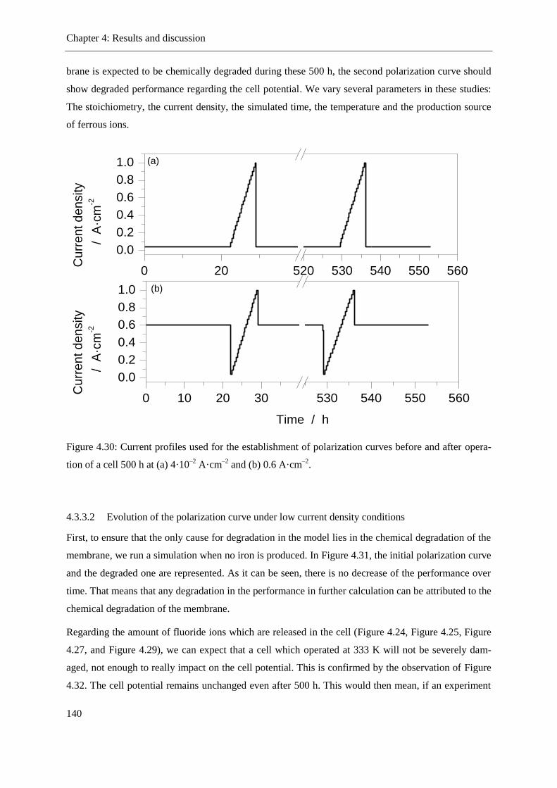
Chapter 4: Results and discussion
140
brane is expected to be chemically degraded during these 500 h, the second polarization curve should
show degraded performance regarding the cell potential. We vary several parameters in these studies:
The stoichiometry, the current density, the simulated time, the temperature and the production source
of ferrous ions.
Figure 4.30: Current profiles used for the establishment of polarization curves before and after opera-
tion of a cell 500 h at (a) 4·10–2
A·cm–2
and (b) 0.6 A·cm–2
.
4.3.3.2 Evolution of the polarization curve under low current density conditions
First, to ensure that the only cause for degradation in the model lies in the chemical degradation of the
membrane, we run a simulation when no iron is produced. In Figure 4.31, the initial polarization curve
and the degraded one are represented. As it can be seen, there is no decrease of the performance over
time. That means that any degradation in the performance in further calculation can be attributed to the
chemical degradation of the membrane.
Regarding the amount of fluoride ions which are released in the cell (Figure 4.24, Figure 4.25, Figure
4.27, and Figure 4.29), we can expect that a cell which operated at 333 K will not be severely dam-
aged, not enough to really impact on the cell potential. This is confirmed by the observation of Figure
4.32. The cell potential remains unchanged even after 500 h. This would then mean, if an experiment
0 10 20 30 530 540 550 560
0.0
0.2
0.4
0.6
0.8
1.0 (b)
Cu
rre
nt
de
nsity
/ A
·cm
-2
Time / h
0 20 520 530 540 550 560
0.0
0.2
0.4
0.6
0.8
1.0
Cu
rre
nt
de
nsity
/ A
·cm
-2
(a)
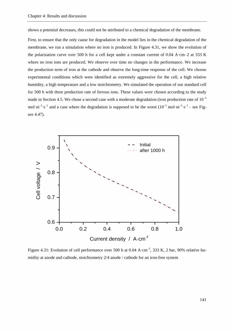
Chapter 4: Results and discussion
141
shows a potential decreases, this could not be attributed to a chemical degradation of the membrane.
First, to ensure that the only cause for degradation in the model lies in the chemical degradation of the
membrane, we run a simulation where no iron is produced. In Figure 4.31, we show the evolution of
the polarization curve over 500 h for a cell kept under a constant current of 0.04 A·cm–2 at 333 K
where no iron ions are produced. We observe over time no changes in the performance. We increase
the production term of iron at the cathode and observe the long-time response of the cell. We choose
experimental conditions which were identified as extremely aggressive for the cell, a high relative
humidity, a high temperature and a low stoichiometry. We simulated the operation of our standard cell
for 500 h with three production rate of ferrous ions. These values were chosen according to the study
made in Section 4.5. We chose a second case with a moderate degradation (iron production rate of 10–5
mol·m–3
·s–1
and a case where the degradation is supposed to be the worst (10–3
mol·m–3
·s–1
– see Fig-
ure 4.47).
Figure 4.31: Evolution of cell performance over 500 h at 0.04 A·cm–2
, 333 K, 2 bar, 90% relative hu-
midity at anode and cathode, stoichiometry 2/4 anode / cathode for an iron-free system
0.0 0.2 0.4 0.6 0.8 1.0
0.6
0.7
0.8
0.9
Ce
ll vo
lta
ge
/
V
Current density / A·cm-2
Initial
after 1000 h
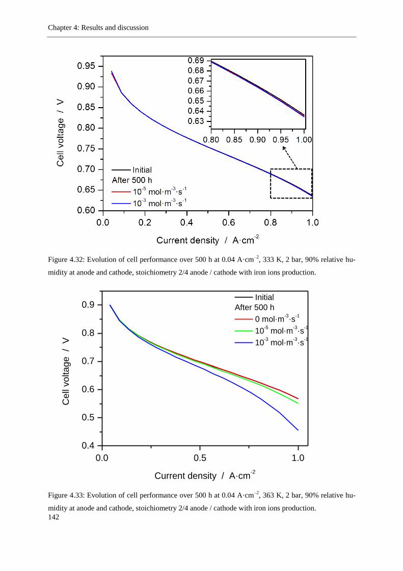
Chapter 4: Results and discussion
142
Figure 4.32: Evolution of cell performance over 500 h at 0.04 A·cm–2
, 333 K, 2 bar, 90% relative hu-
midity at anode and cathode, stoichiometry 2/4 anode / cathode with iron ions production.
Figure 4.33: Evolution of cell performance over 500 h at 0.04 A·cm–2
, 363 K, 2 bar, 90% relative hu-
midity at anode and cathode, stoichiometry 2/4 anode / cathode with iron ions production.
0.0 0.5 1.0
0.4
0.5
0.6
0.7
0.8
0.9 Initial
After 500 h
0 mol·m-3·s
-1
10-5 mol·m
-3·s
-1
10-3 mol·m
-3·s
-1
Cell
volta
ge
/
V
Current density / A·cm-2

Chapter 4: Results and discussion
143
From the observation of Figure 4.33, we see that the impact of the increase of the membrane resistance
on the cell voltage is, under the most aggressive simulated conditions, about 100 mV at 1 A·cm–2
after
500 h. As such conditions of ferrous ions production is quite unrealistic (and because a PEMFC is
never let 500 h in an idle mode), we can say that it is almost unthinkable that a cell fails after 500 h
only because of the chemical degradation of its membrane.
4.3.3.3 Evolution of the polarization curve under higher current density
We may now see how the cell behaves if it operates 500 h under a non-zero load, as this is closer to
reality than idle operating conditions.
In Figure 4.34, we represent the evolution of the polarization curve after 500 h for a cell which operat-
ed at 0.6 A·cm–2
and whose iron production varies. In agreement with the observation of cumulative
fluoride release, the membrane is less degraded if the demanded current is not zero. The voltage losses
are respectively 65.57 mV (high iron production) and 11.21 mV (low iron production) at 1.0 A·cm–2
after 500 h. As previously indicated, these values are given for a cell subject to release a lot of iron in
the cell. If we reduce the production of ferrous ions by two order of magnitude (Figure 4.35), the volt-
age losses are reduced to 15 mV (0.04 A·cm–2
) and 12 mV (0.6 A·cm–2
) at 1.0 A·cm–2
after 500 h.
This represents a reducing of the performance of about 2 %, which remains acceptable for a further
operation of the cell.

Chapter 4: Results and discussion
144
Figure 4.34: Evolution of cell performance over 500 h at 0.6 A·cm–2
, 363 K, 2 bar, 90% relative hu-
midity at anode and cathode, stoichiometry 2/4 anode / cathode with iron ions production
Figure 4.35: Evolution of cell performance over 500 h at 0.04 A·cm–2
and 0.6 A·cm–2
, 363 K, 2 bar,
0.0 0.5 1.0
0.4
0.5
0.6
0.7
0.8
0.9 Initial
After 500 h
0 mol·m-3·s
-1
10-5 mol·m
-3·s
-1
10-3 mol·m
-3·s
-1
Cell
volta
ge
/
V
Current density / A·cm-2
0.0 0.5 1.0
0.4
0.5
0.6
0.7
0.8
0.9 Initial
After 500 h
0 mol·m-3·s
-1
10-5 mol·m
-3·s
-1
10-3 mol·m
-3·s
-1
Solid: 0.04 A·cm-2
Dash: 0.6 A·cm-2
Ce
ll vo
lta
ge
/
V
Current density / A·cm-2

Chapter 4: Results and discussion
145
90% relative humidity at anode and cathode, stoichiometry 2/4 anode / cathode with iron ions produc-
tion.
In Figure 4.35, we compared the two cases we studied. The performances of the cell operated at low
current density are clearly more degraded than the one operated at high current density.
4.3.3.4 Comparison with experiment
We can compare our evolution of polarization curve with experimental data as well. The experiment
mentioned in Section 4.2.2.2 was carried out during over 500h. In Figure 4.36, we report these com-
parisons. Several remarks can be made. As no information can be provided from experimentalists
about the real amount of iron which penetrates the system, the comparison is rather qualitative. First
the OCV did not changed during the test, this means that if a mixed potential was present at the begin-
ning of the experiment, it did not increase with degradation. After 500 h, the potential decreases at 1
A·cm–2
from 579 mV to 527 mV, which means a decrease of 52 mV. This represents the total losses of
the cell, including contribution of all possible degradation sources, like carbon corrosion, platinum
dissolution and membrane degradation.
Figure 4.36: Comparison between modeling results and experimental results for the evolution of the
polarization curve after 500 h at 0.6 A·cm–2
.
0.0 0.2 0.4 0.6 0.8 1.0
0.4
0.5
0.6
0.7
0.8
0.9 Initial modeling
Initial experiment
After 500 h
0 mol·m-3·s
-1
10-5 mol·m
-3·s
-1
10-3 mol·m
-3·s
-1
Experiment
Ce
ll vo
lta
ge
/
V
Current density / A·cm-2

Chapter 4: Results and discussion
146
From the modeling results, we have the possibility to uncorrelate the impact of the membrane degrada-
tion over the whole performance decreases. Assuming an iron ion production of 10–3
mol·m–3
·s–1
, the
voltage drop over 500 h in the experiment would be only attributed to the membrane degradation.
However, several studies show that the main contributor to potential decrease is rather the electrode
degradation [73, 168]. If we consider now a lower iron ion production like 10–5
mol·m–3
·s–1
, we see
that the potential decrease due to the chemical degradation is much lower. Moreover, at that produc-
tion rate and after 500 h, the net weight of iron released in the membrane is 151.2 µg. This value
seems realistic compared to the weight of a bipolar plate.
4.3.4 Localization of the degradation in the membrane
Thanks to its 1D discretization, our model also allows to spatially resolve the state of degradation of
the membrane along its thickness.
We recall that ferrous ions are produced at the cathode side and the hydrogen peroxide at the anode
side. In Figure 4.37, we normalized the concentration of species impacting on chemical degradation of
the cell and plotted their profile along the membrane. We did this normalization in the concentration
because of the high concentration differences observed in the cell (from few nmol·m–3
for radicals up
to 10–1
mol·m–3
for dissolved gases). We observe that the region with the highest concentration is lo-
cated in the middle of the cell, and close to the electrodes, the concentration is the lowest. This means
that the degradation rates exhibit trends higher values close to the electrodes (close to the production
source of the species involved in the membrane degradation) as in the middle of the cell, where the
concentrations are lower. However, the variation of the concentration is too low to really talk about
regions in the vicinity of the electrodes which are more degraded than the middle of the membrane.
We assume this is due to diffusion coefficients of the species in the Nafion®, which have been to the
usually set to standard and maybe over-estimated values when unknown from the literature. Neverthe-
less the model adapted with optimized parameters could then help to explain the phenomenon of
membrane thinning, as displayed in Figure 1.19: the membrane thinning is not linear with the released
fluoride, but reaches a limit even if more fluoride are released by the system. The model could help to
give clues for a understanding of the phenomena. According to Figure 1.19, it may be expected over
time that first anode and cathode side are degraded, inducing a membrane thinning. With continuous
degradation, maybe the diffusion processes could be responsible for a motion of the area of higher
degradation inside the cell, reducing the membrane thinning phenomenon.
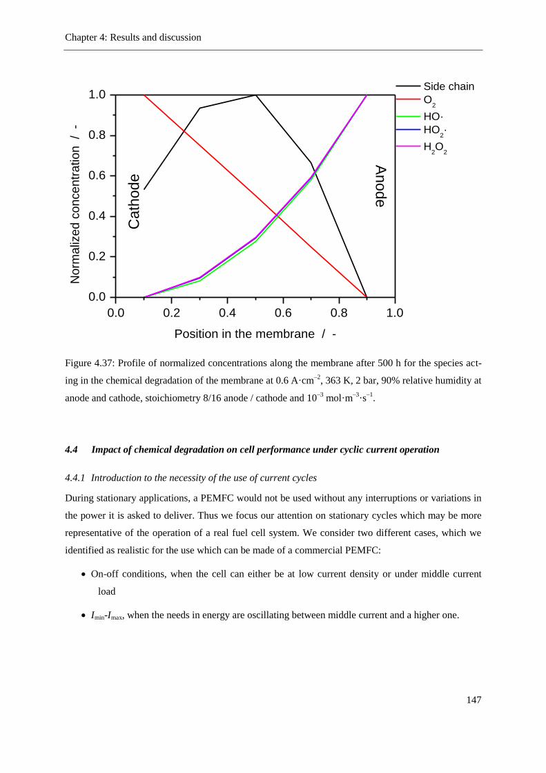
Chapter 4: Results and discussion
147
Figure 4.37: Profile of normalized concentrations along the membrane after 500 h for the species act-
ing in the chemical degradation of the membrane at 0.6 A·cm–2
, 363 K, 2 bar, 90% relative humidity at
anode and cathode, stoichiometry 8/16 anode / cathode and 10–3
mol·m–3
·s–1
.
4.4 Impact of chemical degradation on cell performance under cyclic current operation
4.4.1 Introduction to the necessity of the use of current cycles
During stationary applications, a PEMFC would not be used without any interruptions or variations in
the power it is asked to deliver. Thus we focus our attention on stationary cycles which may be more
representative of the operation of a real fuel cell system. We consider two different cases, which we
identified as realistic for the use which can be made of a commercial PEMFC:
On-off conditions, when the cell can either be at low current density or under middle current
load
Imin-Imax, when the needs in energy are oscillating between middle current and a higher one.
0.0 0.2 0.4 0.6 0.8 1.0
0.0
0.2
0.4
0.6
0.8
1.0 Side chain
O2
HO·
HO2·
H2O
2
Anode
N
orm
aliz
ed
co
nce
ntr
atio
n
/ -
Position in the membrane / -
Cath
ode

Chapter 4: Results and discussion
148
4.4.2 On-off cycle of a PEMFC
4.4.2.1 Description of the cycle
If we imagine a stationary system which is used only during the half of the day (for example power
supply during the night to make up for a solar energy system), the cell will run during several hours
and then be shut down, to be restarted after several hours, as the example displayed in Figure 4.38..
Figure 4.38: Current density profile used to simulate an on - off operation of a PEMFC
4.4.2.2 Behavior of a PEMFC under on-off conditions
We want to see here if the cell responds more like a cell operated under on-off conditions or rather
under 0.6 A·cm–2
. Every 10 hours, the cell is shut down for 10 hours, and then restarted for 10 h.
The evolution of the cell potential is given in Figure 4.39. For simplicity reasons, we illustrate here the
evolution of the reference cases taken as simulations under constant current density as in Section 4.3.
The PEMFC design we simulated is our standard cell with the simulation conditions given in Table
4.11. We can see that the potential remains stable over time and the potential is in agreement to the
reference cases. We notice small overshoots and undershoots when the current density increases, re-
spectively decreases. The source of this behavior is presented in Figure 4.40, where the temporal evo-
lution of the water content in every compartment of the discretization is reported.
0 100 200 300
0.0
0.2
0.4
0.6
Cu
rre
nt
de
nsity
/ A
·cm
-2
Time / h
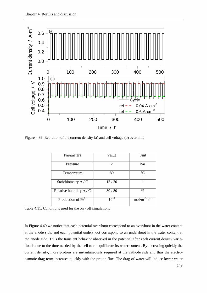
Chapter 4: Results and discussion
149
Figure 4.39: Evolution of the current density (a) and cell voltage (b) over time
Parameters Value Unit
Pressure 2 bar
Temperature 80 °C
Stoichiometry A / C 15 / 20 -
Relative humidity A / C 80 / 80 %
Production of Fe2+
10–3
mol·m–3
·s–1
Table 4.11: Conditions used for the on - off simulations
In Figure 4.40 we notice that each potential overshoot correspond to an overshoot in the water content
at the anode side, and each potential undershoot correspond to an undershoot in the water content at
the anode side. Thus the transient behavior observed in the potential after each current density varia-
tion is due to the time needed by the cell to re-equilibrate its water content. By increasing quickly the
current density, more protons are instantaneously required at the cathode side and thus the electro-
osmotic drag term increases quickly with the proton flux. The drag of water will induce lower water
0 100 200 300 400 500
0.40.50.60.70.80.91.0
Cycle
ref 0.04 A·cm-2
ref 0.6 A·cm-2
(b)
Ce
ll vo
lta
ge
/
V
Time / h
0 100 200 300 400 500
0.0
0.2
0.4
0.6
Cu
rre
nt
de
nsity
/ A
·m-2
(a)
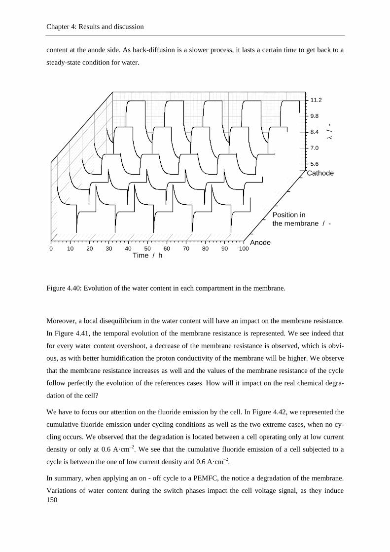
Chapter 4: Results and discussion
150
content at the anode side. As back-diffusion is a slower process, it lasts a certain time to get back to a
steady-state condition for water.
Figure 4.40: Evolution of the water content in each compartment in the membrane.
Moreover, a local disequilibrium in the water content will have an impact on the membrane resistance.
In Figure 4.41, the temporal evolution of the membrane resistance is represented. We see indeed that
for every water content overshoot, a decrease of the membrane resistance is observed, which is obvi-
ous, as with better humidification the proton conductivity of the membrane will be higher. We observe
that the membrane resistance increases as well and the values of the membrane resistance of the cycle
follow perfectly the evolution of the references cases. How will it impact on the real chemical degra-
dation of the cell?
We have to focus our attention on the fluoride emission by the cell. In Figure 4.42, we represented the
cumulative fluoride emission under cycling conditions as well as the two extreme cases, when no cy-
cling occurs. We observed that the degradation is located between a cell operating only at low current
density or only at 0.6 A·cm–2
. We see that the cumulative fluoride emission of a cell subjected to a
cycle is between the one of low current density and 0.6 A·cm–2
.
In summary, when applying an on - off cycle to a PEMFC, the notice a degradation of the membrane.
Variations of water content during the switch phases impact the cell voltage signal, as they induce
0 10 20 30 40 50 60 70 80 90 100
5.6
7.0
8.4
9.8
11.2
Cathode
Time / h
/ -
Anode
Position in
the membrane / -
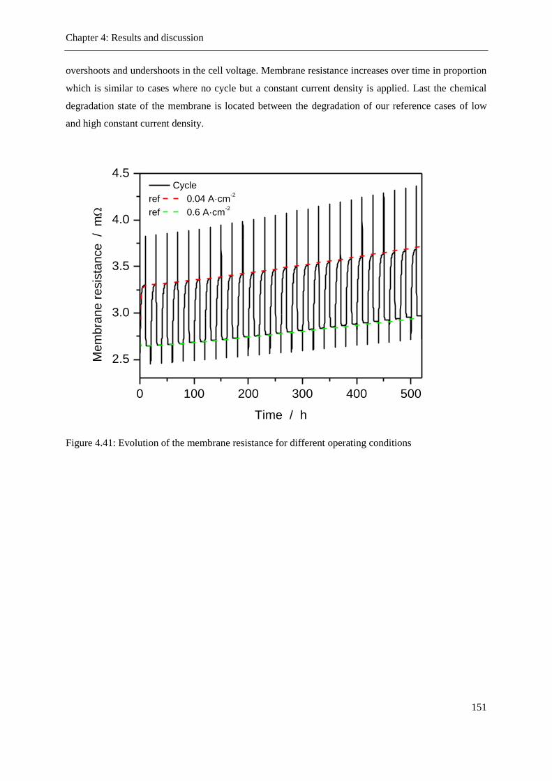
Chapter 4: Results and discussion
151
overshoots and undershoots in the cell voltage. Membrane resistance increases over time in proportion
which is similar to cases where no cycle but a constant current density is applied. Last the chemical
degradation state of the membrane is located between the degradation of our reference cases of low
and high constant current density.
Figure 4.41: Evolution of the membrane resistance for different operating conditions
0 100 200 300 400 500
2.5
3.0
3.5
4.0
4.5 Cycle
ref 0.04 A·cm-2
ref 0.6 A·cm-2
Me
mb
ran
e r
esis
tan
ce
/
m
Time / h

Chapter 4: Results and discussion
152
Figure 4.42: Cumulative fluoride release for different operating conditions
4.4.3 Imin–Imax cycle of a PEMFC
4.4.3.1 Description of the cycle
We focus now on a case when the PEMFC is operated in two different states, either at 0.6 A·cm–2
or at
1.2 A·cm–2
. The profile used and the response of the cell are given in Figure 4.43. It may correspond
to a constant use and peak in the needs of energy because of the switch on of more devices on the
PEMFC stack for example. In Table 4.12, we summarize the conditions used in the simulation. We
managed to run the simulation for more than 500 h, for a severely attacked membrane.
4.4.3.2 Behavior of a PEMFC under Imin–Imax conditions
We take now a closer interest on what would happen if we do not oscillate between low current densi-
ty and 0.6 A·cm–2
but between 0.6 A·cm–2
and 1.0 A·cm–2
. In Figure 4.43, the applied operating condi-
tions and the response of the cell are displayed. To make the comparison easier, we plotted as refer-
ence the cases of constant current density condition. We see, like in the previous case (Section
4.4.2.2), that the cycle condition follows the same behavior as the corresponding constant current. We
0 100 200 300 400 500
0
10
20
Cycle
ref 0.04 A·cm-2
ref 0.6 A·cm-2
Cu
mu
lative
F- r
ele
ase
/
µm
ol·
cm
-2
Time / h
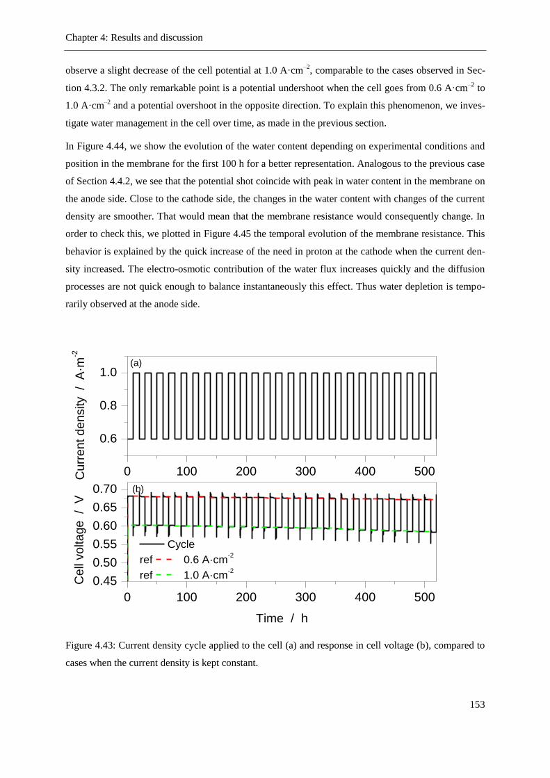
Chapter 4: Results and discussion
153
observe a slight decrease of the cell potential at 1.0 A·cm–2
, comparable to the cases observed in Sec-
tion 4.3.2. The only remarkable point is a potential undershoot when the cell goes from 0.6 A·cm–2
to
1.0 A·cm–2
and a potential overshoot in the opposite direction. To explain this phenomenon, we inves-
tigate water management in the cell over time, as made in the previous section.
In Figure 4.44, we show the evolution of the water content depending on experimental conditions and
position in the membrane for the first 100 h for a better representation. Analogous to the previous case
of Section 4.4.2, we see that the potential shot coincide with peak in water content in the membrane on
the anode side. Close to the cathode side, the changes in the water content with changes of the current
density are smoother. That would mean that the membrane resistance would consequently change. In
order to check this, we plotted in Figure 4.45 the temporal evolution of the membrane resistance. This
behavior is explained by the quick increase of the need in proton at the cathode when the current den-
sity increased. The electro-osmotic contribution of the water flux increases quickly and the diffusion
processes are not quick enough to balance instantaneously this effect. Thus water depletion is tempo-
rarily observed at the anode side.
Figure 4.43: Current density cycle applied to the cell (a) and response in cell voltage (b), compared to
cases when the current density is kept constant.
0 100 200 300 400 500
0.45
0.50
0.55
0.60
0.65
0.70
Cycle
ref 0.6 A·cm-2
ref 1.0 A·cm-2
(b)
Ce
ll vo
lta
ge
/
V
Time / h
0 100 200 300 400 500
0.6
0.8
1.0
Cu
rre
nt
de
nsity
/ A
·m-2
(a)

Chapter 4: Results and discussion
154
Parameters Value Unit
Pressure 2 bar
Temperature 80 °C
Stoichiometry A / C 15 / 20 -
Relative humidity A / C 80 / 80 %
Production of Fe2+
10–3
mol·m–3
·s–1
Table 4.12: Conditions used for the Imin–Imax simulations
Figure 4.44: Evolution of the water content in every compartment of the membrane during Imin–Imax
cycles.
In Figure 4.45, we observe an increase of the membrane resistance over time. To be sure that the
membrane effectively degrades and that the increased resistance is not due to water effect, we plotted
in Figure 4.46 the evolution of the accumulated fluoride concentration in the system for cases which
are treated here. We see that the amount of fluoride ions released during the degradation is between
the extreme of the cycle we applied to the cell. We come then to the same conclusion as for the on -
0 10 20 30 40 50 60 70 80 90 100
5.4
7.2
9.0
10.8
12.6
Cathode
Time / h
/ -
Anode
Position in
the membrane / -
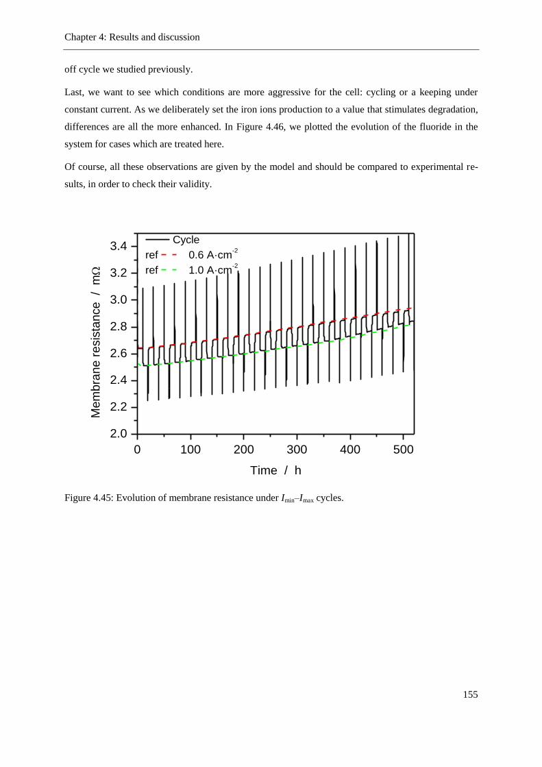
Chapter 4: Results and discussion
155
off cycle we studied previously.
Last, we want to see which conditions are more aggressive for the cell: cycling or a keeping under
constant current. As we deliberately set the iron ions production to a value that stimulates degradation,
differences are all the more enhanced. In Figure 4.46, we plotted the evolution of the fluoride in the
system for cases which are treated here.
Of course, all these observations are given by the model and should be compared to experimental re-
sults, in order to check their validity.
Figure 4.45: Evolution of membrane resistance under Imin–Imax cycles.
0 100 200 300 400 500
2.0
2.2
2.4
2.6
2.8
3.0
3.2
3.4 Cycle
ref 0.6 A·cm-2
ref 1.0 A·cm-2
Me
mb
ran
e r
esis
tan
ce
/
m
Time / h

Chapter 4: Results and discussion
156
Figure 4.46: Cumulative fluoride release for different operation conditions
4.5 Impact of the presence and the amount of iron ions on degradation
As it has been previously mentioned (see in Section 2.3.1 and Section 4.2.3.3), iron ions are the key
parameter for the decomposition of hydrogen peroxide into radicals. Thus we focus in this chapter our
attention on the influence of the presence of iron ions and their concentration on the membrane degra-
dation.
The production of iron ions in the real system can be random and difficult to model. For this reason,
we simulate the degradation behavior of the cell under different production terms of iron ions at the
cathode side. We vary this term in a range from 10–7
up to 1 mol·m–3
·s–1
. As the simulation runs for
500 h or 1000 h, this corresponds to a net release of iron in the membrane (25 cm² and 60µm thick-
ness) from 2.7·10–8
mol up to 2.7·10–1
mol over time or 15 µg to 15g. The upper limit of iron weight in
the membrane is far too high for a real system. This case is then unrealistic, however simulated. It
should be taken as a virtual cell in a system highly subjected to end-plate degradation. We assume that
these ions can neither precipitate in the membrane nor react on any other way than those described in
Section 2.3.1.
In Figure 4.47, we plot the cumulative fluoride release in the membrane after 500 h operation at differ-
0 100 200 300 400 500
0
2
4
6
8
10
12
14
16
18
Cycle
ref 0.6 A·cm-2
ref 1.0 A·cm-2
Cu
mu
lative
F- r
ele
ase
/
µm
ol·
cm
-2
Time / h

Chapter 4: Results and discussion
157
ent temperatures (more simulation parameters in the table embedded in Figure 4.47). We choose a low
current density
Figure 4.47: Dependence of the fluoride production on the iron ions production for different tempera-
tures
Beyond these temperature effect, one particularity of our simulate results have to be noticed. Logic
would expect that if we always increase the production term of iron ions in the membrane, the mem-
brane would be worse and worse degraded and would fail faster (potential collapse, consequence of
short circuit involved by the disappearance of the electrolyte). But in Figure 4.47, we observe a very
interesting phenomenon. Under very aggressive conditions, the membrane is less degraded than under
moderate conditions. This could be a very interesting phenomenon if it were experimentally proved.
We searched for published results that could confirm what we get through simulations.
On the previously mentioned contributions, Kodama et al. presented also results which indicates a
similar trend as our modeling results [158, 159]. They studied the degradation of Nafion® in hydrogen
peroxide. They found out that under very aggressive conditions, the degradation effects are drastically
prevented (see in Figure 4.48).

Chapter 4: Results and discussion
158
Figure 4.48: F- effluent rate from Nafion
® 112 (7.2cm × 7.2cm) in 1wt%H2O2, 100ºC × 8 h with iron
ions [159]
Figure 4.49: Effect of Fe2+
concentration on membrane degradation [37]
Kodama et al. measured the fluoride concentration with an ion-selective electrode. Few years later,
Chen and Fuller investigated through XPS Nafion® degradation and measured the produced fluoride
ions through ion chromatography (IC) [37]. As they studied the impact of the ferrous ions concentra-
tion, they observed the same trend as Kodama (Figure 4.49). This trend was criticized by Schiraldi et
al., and assumed to be an experimental error due to the existence of Fe3+
in Fenton’s reagent when
using commercial ion-selective electrodes [31, 37]. This argument was refuted by Chen and Fuller,
responding that such an error could not occur in their experiment using IC. They rather thought that
the observed decreasing in the fluoride production was due to the presence, at high concentration of
Chapter 4: Results and discussion
159
iron ions, of macromolecules containing bound fluoride as degradation products, which could not be
measured by IC. On the contrary, lower concentrations of iron ions would rather lead to fluoride ions
as main degradation product, explaining the difference they observed.
In our model, we consider only one degradation product: fluoride ions. Thus the explanation given by
Chen and Fuller could not be the reason for our observations. This observation has to be a conse-
quence of the model assumptions. Lower membrane degradation means either that less radicals have
been produced by the cell, or the radicals did not react with the side chains themselves but with other
species in the membrane. This is the first step to the explanation we propose for this iron dependence
on the degradation of a PFSA membrane.
If we consider that the hydrogen peroxide production is independent of the concentration of iron ions,
which is logical, Reaction 2.4 cannot be the source of the protection of the membrane against radicals.
However, if we have a look at Reaction 2.5, HO radicals can react with ferrous ions in acidic media to
form ferric ions and water. This leads us to think that if the concentration of iron ions is too high, it
will be easier for the radicals to react with them than attacking the side chain of the membrane.
The typical side chain concentration we used in our simulation is 1200 mol·m–3
. If we look in Figure
4.47, we locate a maximal chemical degradation of the membrane for an iron ions production of about
10–3
mol·m–3
·s–1
. After the 500 h of our simulations, this would mean a net concentration of iron ions
of 10–3
·500·3600 = 1800 mol·m–3
. We assume then that when the total concentration of iron ions in-
troduced into the system is close to the initial concentration of side chain, the degradation is maximal.
Beyond this point, the iron ion concentration will progressively hidethe side chain and prevent the
radical attack on the membrane. More calculation should be carried out to justify this hypothesis, for
example by increasing the simulation time and seeing if our hypothesis is correct.
A second hypothesis which can be made is related to the production of hydrogen peroxide at the an-
ode. If iron ions and H2O2 are produced at similar rates, ferrous ions will not have the possibility to
accumulate and the radicals will react with the membrane.
If iron ions are produced slower than H2O2, H2O2 will not be completely decomposed into radicals,
leading to a decelerated attack on the membrane.
If irons ions are produced much faster than H2O2, H2O2 will be completely decomposed and ferrous
ions will be available for further reaction with the produced radicals. If the concentration of ferrous
ions becomes too high, the radicals will preferentially react with iron than with the membrane, which
will protect it.
In Figure 4.50, our hypothesis is confirmed. We observe that for a low production of Fe2+
, hydrogen
peroxide is more present in the membrane and the rate of degradation increases. When we pass the
limit of 10–2
mol·m–3
·s–1
the concentration of iron ions severely increases and this corresponds to the

Chapter 4: Results and discussion
160
point where the membrane degradation slows down. That would then confirm our second hypothesis.
Figure 4.50: Simulated evolution of the concentration of different species during degradation (500h,
low current density, 363 K).
We can notice in this study that the chemical degradation of a PFSA membrane is strongly tempera-
ture dependent. Even if lower temperatures do not provide as good performances as higher tempera-
ture, the durability of the membrane is improved. According to our simulations, running a cell at 60 °C
instead of 90 °C could reduce the chemical degradation by a factor 4, which is not negligible.
Moreover, in a cell severely polluted by ferrous ions, the chemical degradation which we simulate is
close to zero. However, ferrous ions have a high affinity to the side chain of the PFSA membrane,
which is currently not taken into account in our present model. Thus the negative impact of iron ions
on the conductivity of the membrane is not regarded. But from a chemical stability point of view, it
seems that in presence of hydrogen peroxide and a high quantity of iron ions, Nafion® is more chemi-
cally stable than in moderate conditions.
4.6 Degradation of other PFSA membranes
Until now, all the simulations we made used parameters of Nafion®. Even if Nafion
® has been a stand-
1E-8 1E-7 1E-6 1E-5 1E-4 1E-3 0.01 0.1 1 10
1E-14
1E-12
1E-10
1E-8
1E-6
1E-4
0.01
1
100
10000
1000000
Species
F-
Fe2+
Fe3+
H2O
2
HO·
HO2·
Co
nce
ntr
atio
n
/ m
ol·
m-3
Fe2+
production / mol·m-3·s
-1

Chapter 4: Results and discussion
161
ard in fuel cell technology, providing gas impermeability, a good thermal, mechanical and chemical
stability and a high proton conductivity, many other products came over the years on the market of
electrolytes for low–temperature PEMFC (see Table 1.2). They are all PFSA membranes, but they
differ in the chemical structure (equivalent weight, length of side chain). Thus the F / S ratio “41”
which was used in the model for the Nafion® description would not suit to a membrane with shorter
side chains, for example like Aquivion (Figure 4.4), whose equivalent weight is also lower than for
Nafion®.
With help of the data from Table 1.2, we run simulations with different kind of PFSA membrane, to
see how the chemical structure impact on the chemical degradation of the membrane. This was made
under the assumption that the kinetic rate of attack of radicals on the ether functions bonding side
chains to the back bone is independent of the chemical structure. This could only be checked by per-
forming experiments with several membranes and following the fluoride emission rate.
In Table 4.13, we present the membrane parameters that we used in our study. We want to determine,
under constant current conditions, which membrane is the most resistant to chemical degradation. The
calculation of the ratios F / S was performed considering a general structure for PFSA membranes as
shown in Figure 1.3 and the (m, n, x, y) values given in Table 1.2.
Membrane EW / g·eq–1
Ratio F / S Thickness / µm
Aciplex 1100 20 25
Dow 800 14 125
Aquivion 870 35 30
Nafion® 1100 41 60
Table 4.13: Parameters of membranes simulated in this study
For this study, we can separate membranes into several classes:
Low and high equivalent weight
Low and high fluoride content
Under these points, we sort out as:
Aciplex: High EW, low F / S ratio
Dow: Low EW, low F / S ratio
Aquivion: Low EW, high F / S ratio
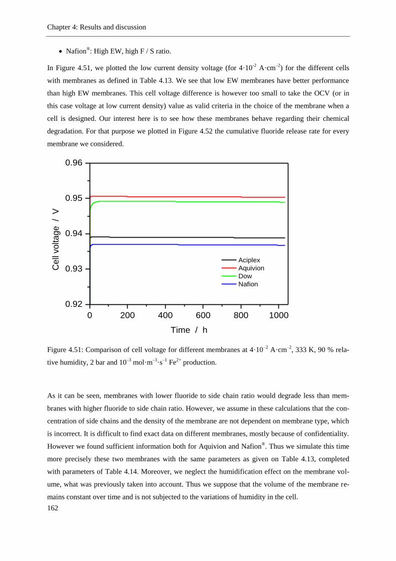
Chapter 4: Results and discussion
162
Nafion®: High EW, high F / S ratio.
In Figure 4.51, we plotted the low current density voltage (for 4·10-2
A·cm–2
) for the different cells
with membranes as defined in Table 4.13. We see that low EW membranes have better performance
than high EW membranes. This cell voltage difference is however too small to take the OCV (or in
this case voltage at low current density) value as valid criteria in the choice of the membrane when a
cell is designed. Our interest here is to see how these membranes behave regarding their chemical
degradation. For that purpose we plotted in Figure 4.52 the cumulative fluoride release rate for every
membrane we considered.
Figure 4.51: Comparison of cell voltage for different membranes at 4·10–2
A·cm–2
, 333 K, 90 % rela-
tive humidity, 2 bar and 10–3
mol·m–3
·s–1
Fe2+
production.
As it can be seen, membranes with lower fluoride to side chain ratio would degrade less than mem-
branes with higher fluoride to side chain ratio. However, we assume in these calculations that the con-
centration of side chains and the density of the membrane are not dependent on membrane type, which
is incorrect. It is difficult to find exact data on different membranes, mostly because of confidentiality.
However we found sufficient information both for Aquivion and Nafion®. Thus we simulate this time
more precisely these two membranes with the same parameters as given on Table 4.13, completed
with parameters of Table 4.14. Moreover, we neglect the humidification effect on the membrane vol-
ume, what was previously taken into account. Thus we suppose that the volume of the membrane re-
mains constant over time and is not subjected to the variations of humidity in the cell.
0 200 400 600 800 1000
0.92
0.93
0.94
0.95
0.96
Aciplex
Aquivion
Dow
Nafion
Ce
ll vo
lta
ge
/
V
Time / h

Chapter 4: Results and discussion
163
Membrane Side chain concentration / mol·m–3
Density / kg·m–3
Aquivion 2367 2060
Nafion® 1800 2240
Table 4.14: Extra parameters regarded for the accurate study of the influence of membrane type.
Figure 4.52: Comparison of cumulative fluoride production for different membranes at 4·10–2
A·cm–2
,
333 K, 90 % relative humidity, 2 bar and 10–3
mol·m–3
·s–1
Fe2+
production.
In Table 4.14, the initial concentration of side chain is calculated as the ratio between the density of
the membrane and the equivalent weight. As we observe, a decrease of the EW will increase the con-
centration of side chain and as Aquivion contains less fluoride than Nafion®, it may be comprehensible
that the polymer has a lighter densityas well.
The results of our simulation concerning the membrane degradation are given in Figure 4.53 (b). In
Figure 4.53 (a), we report for comparison the results for membranes considering the first assumptions
we made. What we notice in that case, is that the chemical degradation of both membranes is similar.
We observe that with real membrane parameters, the degradation behavior is strongly impacted. When
in the simple case we only changed one single parameter, we should have seen more precisely the
0 200 400 600 800 1000
0
2
4
6
8
10
12
14 Aciplex
Aquivion
Dow
Nafion
Cu
mu
lative
F- r
ele
ase
/
µm
ol·
cm
-2
Time / h

Chapter 4: Results and discussion
164
physical properties of membranes, which remain sometimes very difficult to access.
Figure 4.53: Comparison of cumulative fluoride production for different membranes at 4·10–2
A·cm–2
,
363 K, 90 % relative humidity, 2 bar and 10–3
mol·m–3
·s–1
Fe2+
production (a) Simple case and (b)
Complete case.
The chemical degradation of Nafion® 112 and Aquivion E87-03 is comparable. Over 1,000 h, they
seem to degrade at similar rates, but physical properties of Aquivion should to make it more resistant
to radicals attack, according to our model’s prediction. As mentioned in Section 1.2, PFSA membranes
are really complex objects whose study requires the best technology available. It cannot be summa-
rized to a simple model to ascertain on their resistance against chemical degradation. However, this
trend could be experimentally observed. As manufacturers aim on producing more resistant products
with same performance, it may be expected that in a few years, the results we obtained through simu-
lation exaggerate the real trend. But in that case, the degradation mechanism would remain the same
and only kinetics parameters might change, assuming known membrane properties.
4.7 Prediction of long-term cell durability
In the previous sections, we have presented our simulation results upon the chemical degradation of
0 200 400 600 800 1000
0
10
20
30(b)
Cu
mu
lative
F- r
ele
ase
/ µ
mo
l·cm
-2
Time / h
0 200 400 600 800 1000
0
5
10
15
Aquivion
Nafion
Cu
mu
lative
F- r
ele
ase
/ µ
mo
l·cm
-2(a)

Chapter 4: Results and discussion
165
the single cell over 500 h, a duration which is reasonable at the laboratory scale, but still too short for a
real stationary application. As the chemical degradation induces a decrease of the cell potential, we
want now to evaluate the time needed for the cell potential to decrease to a point when the cell is con-
sidered as failed (durability). Different criteria can be taken for the durability of the cell. In our current
study, we define the “end-of-life” (EoL) of the cell as the loss of 5% of the initial cell potential (poten-
tial after 20 h).
In Figure 4.54, we display the evolution of the durability with current density and temperature. We
observe that the resistance increases and the durability decreases as the temperature increases. Another
interesting feature is that the durability decreases as the current density increases.
We see as well that increased current density will shorten the durability of the cell.
Figure 4.54: Evolution of durability and membrane resistance at EoL with current density and temper-
ature.
As the cell voltage decrease is due to an increase of the ohmic resistance, it is interesting to check the
evolution of the cell resistance. As we can see in Figure 4.54, no direct correlation can be made be-
tween the membrane resistance at EoL when the durability criterion is reached and the durability of
the cell. At high temperature, the membrane resistance decreases with increasing current density when
the durability criterion is reached. However at low temperature, the membrane resistance increases.
From this, it cannot be concluded that the membrane degradation is more significant at higher current
0.6 0.8 1.0
0
2000
4000
6000
8000
10000
12000
14000
16000
18000 333 K
343 K
353 K
363 K
Current density / A·cm-2
Du
rab
ility
/
h
2.8
3.0
3.2
3.4
3.6
3.8
4.0
4.2
Me
mb
ran
e r
esis
tan
ce
/
m
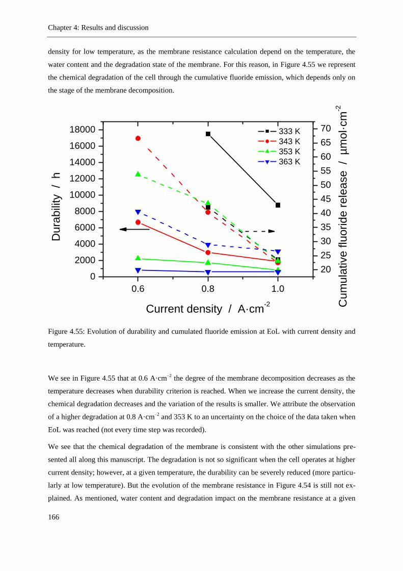
Chapter 4: Results and discussion
166
density for low temperature, as the membrane resistance calculation depend on the temperature, the
water content and the degradation state of the membrane. For this reason, in Figure 4.55 we represent
the chemical degradation of the cell through the cumulative fluoride emission, which depends only on
the stage of the membrane decomposition.
Figure 4.55: Evolution of durability and cumulated fluoride emission at EoL with current density and
temperature.
We see in Figure 4.55 that at 0.6 A·cm–2
the degree of the membrane decomposition decreases as the
temperature decreases when durability criterion is reached. When we increase the current density, the
chemical degradation decreases and the variation of the results is smaller. We attribute the observation
of a higher degradation at 0.8 A·cm–2
and 353 K to an uncertainty on the choice of the data taken when
EoL was reached (not every time step was recorded).
We see that the chemical degradation of the membrane is consistent with the other simulations pre-
sented all along this manuscript. The degradation is not so significant when the cell operates at higher
current density; however, at a given temperature, the durability can be severely reduced (more particu-
larly at low temperature). But the evolution of the membrane resistance in Figure 4.54 is still not ex-
plained. As mentioned, water content and degradation impact on the membrane resistance at a given
0.6 0.8 1.0
0
2000
4000
6000
8000
10000
12000
14000
16000
18000 333 K
343 K
353 K
363 K
Current density / A·cm-2
Du
rab
ility
/
h
20
25
30
35
40
45
50
55
60
65
70
Cu
mu
lative
flu
orid
e r
ele
ase
/ µ
mo
l·cm
-2
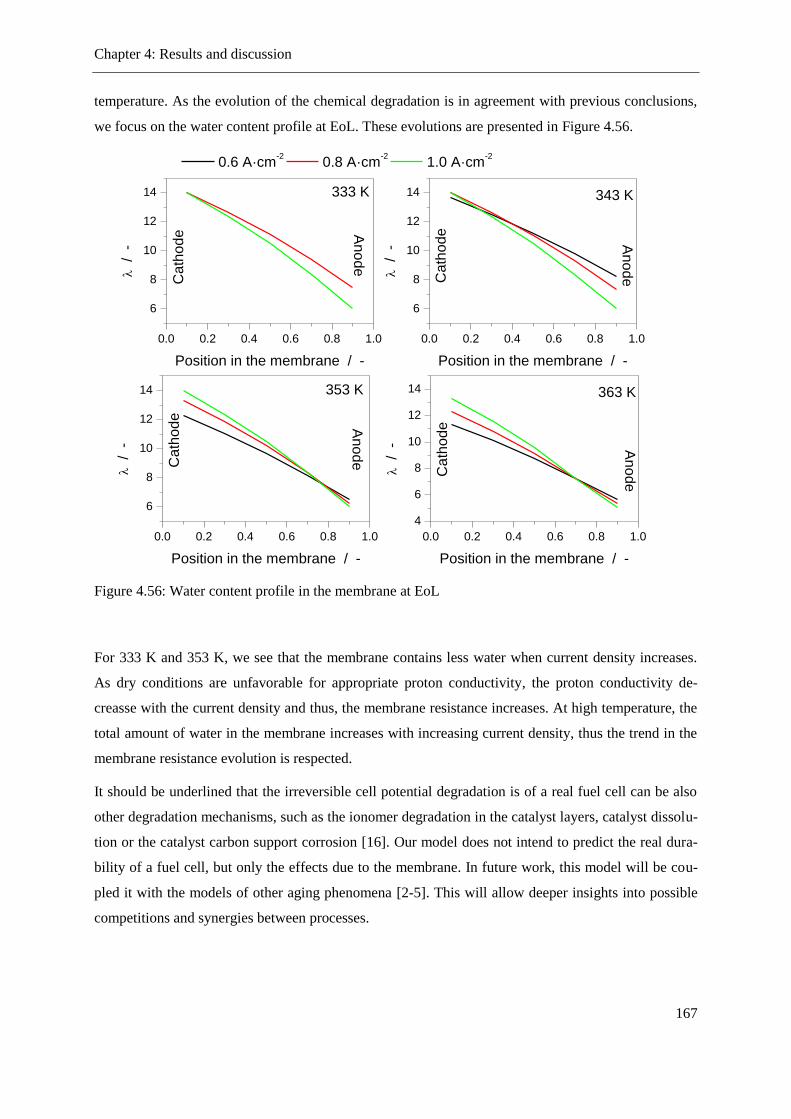
Chapter 4: Results and discussion
167
temperature. As the evolution of the chemical degradation is in agreement with previous conclusions,
we focus on the water content profile at EoL. These evolutions are presented in Figure 4.56.
Figure 4.56: Water content profile in the membrane at EoL
For 333 K and 353 K, we see that the membrane contains less water when current density increases.
As dry conditions are unfavorable for appropriate proton conductivity, the proton conductivity de-
creasse with the current density and thus, the membrane resistance increases. At high temperature, the
total amount of water in the membrane increases with increasing current density, thus the trend in the
membrane resistance evolution is respected.
It should be underlined that the irreversible cell potential degradation is of a real fuel cell can be also
other degradation mechanisms, such as the ionomer degradation in the catalyst layers, catalyst dissolu-
tion or the catalyst carbon support corrosion [16]. Our model does not intend to predict the real dura-
bility of a fuel cell, but only the effects due to the membrane. In future work, this model will be cou-
pled it with the models of other aging phenomena [2-5]. This will allow deeper insights into possible
competitions and synergies between processes.
0.0 0.2 0.4 0.6 0.8 1.0
6
8
10
12
14
Ca
tho
de
Ca
tho
de
/ -
Position in the membrane / -
Ca
tho
de
333 K
0.0 0.2 0.4 0.6 0.8 1.0
6
8
10
12
14 343 K
0.6 A·cm-2
0.8 A·cm-2
1.0 A·cm-2
An
od
e
An
od
eC
ath
od
e
/ -
Position in the membrane / -
0.0 0.2 0.4 0.6 0.8 1.0
6
8
10
12
14 353 K
An
od
e
/ -
Position in the membrane / -
0.0 0.2 0.4 0.6 0.8 1.0
4
6
8
10
12
14 363 K
An
od
e
/ -
Position in the membrane / -
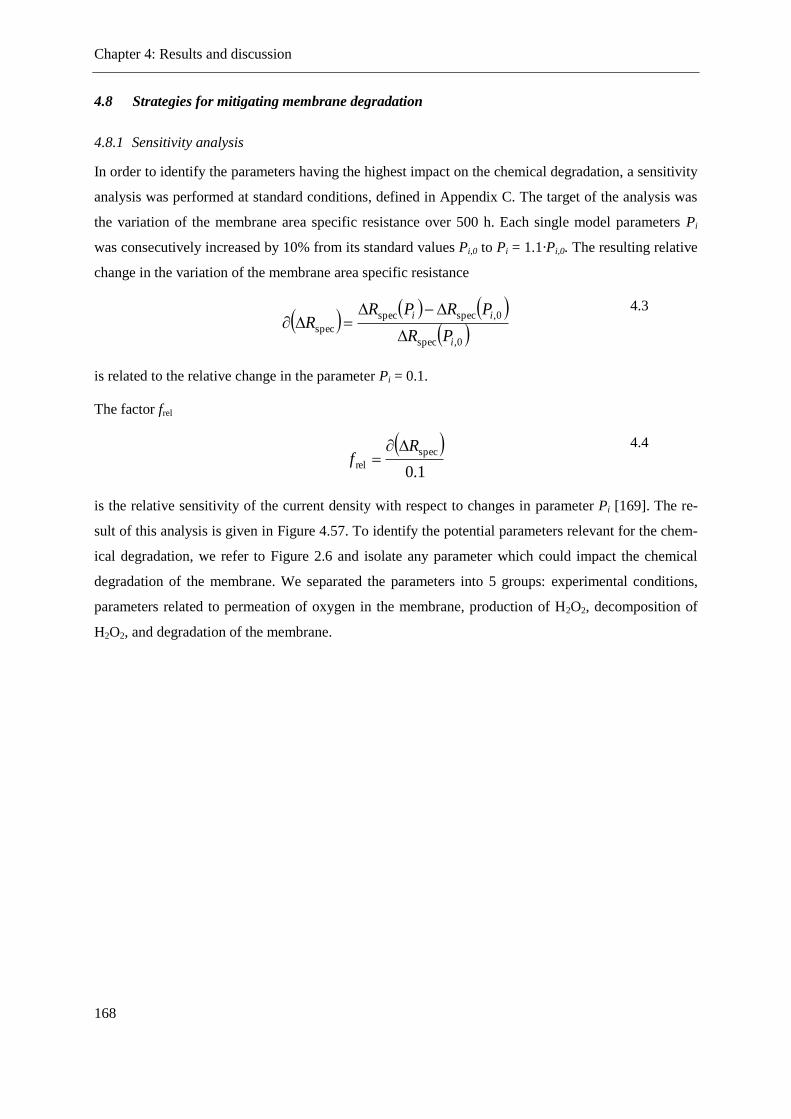
Chapter 4: Results and discussion
168
4.8 Strategies for mitigating membrane degradation
4.8.1 Sensitivity analysis
In order to identify the parameters having the highest impact on the chemical degradation, a sensitivity
analysis was performed at standard conditions, defined in Appendix C. The target of the analysis was
the variation of the membrane area specific resistance over 500 h. Each single model parameters Pi
was consecutively increased by 10% from its standard values Pi,0 to Pi = 1.1·Pi,0. The resulting relative
change in the variation of the membrane area specific resistance
,0spec
,0specspec
spec
i
ii
PR
PRPRR
4.3
is related to the relative change in the parameter Pi = 0.1.
The factor frel
1.0
spec
rel
Rf
4.4
is the relative sensitivity of the current density with respect to changes in parameter Pi [169]. The re-
sult of this analysis is given in Figure 4.57. To identify the potential parameters relevant for the chem-
ical degradation, we refer to Figure 2.6 and isolate any parameter which could impact the chemical
degradation of the membrane. We separated the parameters into 5 groups: experimental conditions,
parameters related to permeation of oxygen in the membrane, production of H2O2, decomposition of
H2O2, and degradation of the membrane.

Chapter 4: Results and discussion
169
Figure 4.57: Sensitivity analysis of our chemical degradation model. A positive sensitivity means that
an increase of the parameter increases the degradation. A value of 1.0 means that the area specific
resistance degradation is directly proportional to the parameter.
Experimental conditions – We investigate the effect of temperature, pressure, relative humidity in the
electrode and stoichiometry of the gases. Relative humidities have almost a direct proportionality with
the evolution of the membrane area specific resistance. The stoichiometry of the gases and pressure
variations has a small impact on the resistance variation. However, temperature has an important im-
pact on the evolution of the cell resistance, which can be explained by temperature dependence of the
kinetic parameters.
Permeation of oxygen through the membrane – For this process we pay particular attention on the two
steps involved in the diffusion of dissolved oxygen within the membrane. The model presents a quasi-
linearity between degradation and both, Henry’s constant for the dissolution of oxygen from the gas
phase into the water of the membrane and the diffusion coefficient of dissolved oxygen within the
membrane.
Production of H2O2 – We vary here the different reaction rate constants of the steps of hydrogen per-
oxide production (forward and backward reactions). The influence of these rates is relatively small and
no significant impact in the change of the membrane area specific resistance is noticed.
-1.0 -0.5 0.0 0.5 1.0
-1.07
Sensitivity of Rmemb
spec (f
rel)
Experimental conditions
Temperature
Pressure
Relative humidity anode
Relative humidity cathode
Stoichiometry anode
Stoichiometry cathode
Permeation of O2
Diffusion coefficient O2
Henry constant O2
Production of H2O
2
Reaction 4.6 forward
Reaction 4.6 backward
Reaction 4.7 forward
Reaction 4.7 backward
Reaction 4.8 forward
Reaction 4.8 backward
Reaction 4.9 forward
Reaction 4.9 backward
Decomposition of H2O
2
Reaction 3.1
Reaction 3.2
Reaction 3.3
Reaction 3.4
Reaction 3.5
Diffusion coefficient H2O
2
Membrane degradation
Degradation rate constant
Production Fe2+
8.05
1.031.56
1.03
1.07

Chapter 4: Results and discussion
170
Decomposition of H2O2 into radicals – We focus here on the Fenton reactions within the chemical
degradation model, the production rate of iron ions and the diffusion of hydrogen peroxide in the
membrane. The diffusion coefficient of hydrogen peroxide has a proportional impact on the membrane
area specific resistance degradation. Regarding Fenton steps, Reaction 2.1, Reaction 2.4 and Reaction
2.5 are rate determining for the variation of membrane area specific resistance. Modifications in the
iron ions production rate show no significant impact on the evolution of the resistance. However it has
to be noticed that this conclusion had to be correlated with Figure 4.47, as depending on the initial
conditions, an increased iron production can induce either a smaller or a larger degradation.
Decomposition of the membrane – The only parameter implied in the radical attack on the PFSA
membrane is the reaction rate constant associated to the attack of the side chain by radicals. It shows
proportionality with the evolution of the membrane specific area resistance.
To conclude, cell temperature is the key parameter to be regarded in membrane chemical degradation.
Increased temperature has a severe impact on the degradation of the membrane. However, increased
relative humidity at the cathode side will reduce the chemical degradation on a proportional way. Re-
garding steps involved in membrane chemical degradation, dissolution of oxygen and diffusion steps
(both oxygen and hydrogen peroxide) show a certain influence on the chemical degradation of the cell.
Reducing the diffusion coefficient of oxygen by 10 % would for example be enough to reduce the
degradation by 10 % as well. At last, the degradation rate constant of the radical attack on the side
chain is important to be reduced, as it is a key factor of the chemical degradation of the membrane.
4.8.2 Experimental conditions preventing the PFSA membrane chemical degradation
We performed a large set of simulations. Several simulations parameters were analyzed and thus, we
are able to propose optimized conditions, to prevent a membrane from the chemical degradation and
thus, help to solve one potential problem for the cell.
All the experimental parameters are in continuous interaction, but on the basis of our model, water
management is the key aspect to control the operation of the cell and thus to optimize performance and
lifetime of the PEMFC. High relative humidity will confer the cell a good humidification, improving
transport processes (proton conduction) but improving gas permeation as well between the electrodes,
what would imply a higher chemical degradation. A too low relative humidity, on the contrary, will
inhibit the proton conduction and moreover the membrane is highly susceptible to dry out, which
would mean mechanical failures, which are not taken here into account but have to be kept in mind
[170].
According to the laws of kinetics, an increase of the temperature accelerates the kinetics of reactions.
This is true unfortunately for both the reactions useful for the cell and the parasitic reactions (inducing

Chapter 4: Results and discussion
171
the degradation). Moreover, temperature strongly impacts the water management of the cell, as its
increases the saturation pressure of vapor as well. That means that it is more difficult at high tempera-
ture for vapor to condense and humidify the membrane. This induces a lower level of humidification
of the membrane and lower performances, as the water content is directly related to the proton conduc-
tivity. Usually, PEMFCs are used at 70 – 80 °C. It appears according to our simulations that it is a
good compromise as well.
A further parameter we analyzed is the iron ions production rate in the system. Iron is a cheap material
which is used in numerous parts of the cell. It may be the main element of the bipolar plates, coated
with gold or a layer of polymer. Our assumption is that defects in the coating are responsible for the
possible corrosion of bipolar plate by water at the cathode side, where the cell potential is high. For a
weak to moderate degradation of the plate, the chemical degradation of the PEM will drastically in-
crease, causing irreversible damages to the membrane. If the plate is severely attacked then it is possi-
ble that the cause of the failure of the cell would not be the membrane degradation but a failure of
bipolar plates. Thus the use of iron-free bipolar plate (for example graphite) should prevent and even
inhibit the formation of radicals and thus the membrane degradation.
4.8.3 Operating conditions for a higher durability of the PFSA membrane
In our simulations, we regarded two different types of dynamic cycles which are usually applied on
test bench to PEMFC: One oscillating between a low and a moderate operating point and the other
between moderate and high current density operating conditions. In each case, the degradation of the
membrane is moderate compared to reference cases when the membrane is run several hundreds of
hours at a constant low current density.
These cycles therefore do not really have an impact on the chemical degradation of the cell. But quick
changes in the current density induce an unbalanced water profile in the membrane for short durations.
This could have a negative impact not on the membrane degradation itself but on other degradation
phenomena occurring at the anode side.
4.8.4 Type of membranes which are the less sensitive to chemical degradation
As mentioned in Section 4.6, the resistance of PFSA membranes is independent of the choice of the
membrane. However, relying of our study on well-parameterized membranes, we propose the use of
PFSA membranes with low EW and fluoride content for PEMFC technology. They are less susceptible
of being degraded. In Figure 4.58, we present the possible interactions between the key parameters
which can be adjusted by the design of a new generation of membrane.
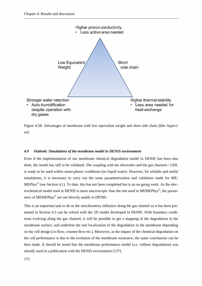
Chapter 4: Results and discussion
172
Figure 4.58: Advantages of membrane with low equivalent weight and short side chain (like Aquivi-
on)
4.9 Outlook: Simulations of the membrane model in DENIS environment
Even if the implementation of our membrane chemical degradation model in DENIS has been also
done, the model has still to be validated. The coupling with the electrodes and the gas channels / GDL
is ready to be used within mono-phasic conditions (no liquid water). However, for reliable and useful
simulations, it is necessary to carry out the same parameterization and validation made for ME-
MEPhys® (see Section 4.1). To date, this has not been completed but is an on-going work. As the elec-
trochemical model used in DENIS is more macroscopic than the one used in MEMEPhys®, the param-
eters of MEMEPhys® are not directly usable in DENIS.
This is an important task to do as the stoichiometry influence along the gas channel as it has been pre-
sented in Section 4.3 can be solved with the 2D model developed in DENIS. With boundary condi-
tions evolving along the gas channel, it will be possible to get a mapping of the degradation in the
membrane surface, and underline the real localization of the degradation in the membrane depending
on the cell design (co-flow, counter-flow etc.). Moreover, as the impact of the chemical degradation on
the cell performance is due to the evolution of the membrane resistance, the same conclusions can be
then made. It should be noted that the membrane performance model (i.e. without degradation) was
already used in a publication with the DENIS environment [137].

Chapter 5: Summary and conclusions
173
CHAPTER 5
Summary and conclusions
5 Summary and conclusions
Degradation of PEMFCs is one of the main issues of this promising technology. The durability of a
PEMFC system is influenced by the irreversible materials degradation phenomena occurring in the
components of the cell; therefore, a detailed understanding of the degradation mechanisms is required
in order to design more durable cell components. These phenomena can have different origins and
consequences and this PhD thesis focused on the chemical degradation of the membrane. There is
strong experimental evidence for changes in the membrane structure during the cell operation (e.g.
thinning by SEM, release of degradation by-products such as organic fragments from the membrane or
fluoride ions in outlet water of the cell) and its proton conductivity loss over time.
In order to simulate the membrane behavior within a complete PEMFC, the membrane model is nu-
merically connected with pre-existing models describing in a detailed way the processes occurring
within the electrodes, the GDLs and the gas channels, within the software tool developed by Franco et
al. at CEA (MEMEPhys® model). The membrane model was developed in a modular and flexible way
in order to be easily embeddable in other simulation software, such as the DENIS package developed
by Bessler et al. at DLR.
Because the membrane resistance is strongly influenced by the fluctuations of relative humidity in the
GDLs, the evolution of membrane resistance on short time scales cannot be reliably considered as a
sign for the chemical degradation of the membrane. One unambiguous sign of chemical degradation,
which is also widely reported in literature, is the presence of fluoride ions in the water evacuated out
of the cell. Consequently, we have simulated fluoride release as one of the major indicators of degra-
dation.
We parameterized and validated our performance and degradation model using available experimental
data from literature. The degradation model shows good agreement with experimental data regarding
the production of hydrogen peroxide (in dependence to the membrane thickness as well), the produced
radicals coming from the decomposition of hydrogen peroxide, and the amount of fluoride ions pro-
Chapter 5: Summary and conclusions
174
duced through the degradation of the membrane through radical attack. This constituted the basis of
detailed parameter studies we presented, showing that the experimental conditions (e.g. gas stoichiom-
etry, relative humidity and temperature) have a strong influence on the degradation. We highlighted
the importance of each condition under different working conditions.
Based on our study of behavior of a cell under constant current load at different temperatures, we no-
ticed that when keeping the relative humidity of the cell constant at each temperature, the degradation
increases as the temperature increases. If the applied current increased, the performance degradation
decreases, and, according to the model, is even inexistent at lower temperature. As the model allowed
1D spatial resolution within the membrane, we could identify the location of more or less severe deg-
radation. Under our assumptions (hydrogen peroxide produced at the anode, iron ions at the cathode),
less degradation was found in the center of the membrane, while the boundaries towards the electrodes
were more degraded. The difference remains however small, as the membrane we simulated as refer-
ence case was thin.
We then simulated conditions where the current load periodically oscillated between two values. As it
could be expected, the degradation of this mix of two states was about in the middle of degradation of
the two extreme cases, where the cell would be run over the same time at a constant current load. This
indicates that dynamic operation does not impact the chemical degradation in comparison to stationary
operation The plots of the cell voltage under periodic switching of current density showed overshoots
and undershoots. The model suggested that these effects were due to local imbalance of the water con-
tent. This causes variations in the membrane resistance, and thus impacts the cell potential.
We further studied the influence of the concentration of iron ions on the degradation. We found out
under all the simulation conditions used that when the production of iron ions thus increased, the
chemical degradation, after having increased to a maximum value, becomes less for highly corroded
system. The explanations we proposed for this behavior was either a relationship between the concen-
tration of side chain in the cell and the one of free iron ions, or that the radicals react another way than
with side chain, so that the membrane is being protected.
The model can be applied to any type of PFSA membrane, as long as the chemical structure and the
physicals properties (thickness, equivalent weight, and density) are known. We compared four differ-
ent PFSA membranes available on the current market. They differed in equivalent weight (low or
high) and side chain length (short or long). The prediction of the model allows us to suggest that re-
garding the instantaneous performances, membranes with lower equivalent weight offers higher per-
formance. Regarding the chemical degradation, membranes with shorter side chains are less subjected
of being degraded, thus would be more stable over time.
Long-term experiments were also simulated. We run the cell for 20,000 h at middle and high current

Chapter 5: Summary and conclusions
175
density and at different temperatures. We fixed as end-of-life condition an arbitrary decrease of 5 % of
the initial cell voltage. It came out that the durability decreases with increased temperature and current
density. As we considered only chemical degradation of the membrane, the cell potential decrease is
due to an increase of the ohmic loss in the membrane. This explained that high current trend to reduce
the durability of the cell, even if our simulations showed in these cases that the membrane degraded
less than at end of life at lower current density.
Regarding the mitigation of the membrane chemical degradation, we concluded that the most im-
portant parameter is the temperature at which the cell is operated. The higher the temperature, the
more severe is the chemical degradation of the membrane. Humidifications of the gases are relevant as
well in the reduction of the chemical degradation. At high relative humidity, the chemical degradation
decreases. Moreover, oxygen dissolution and diffusion in the membrane are a key parameter in the
degradation as well. As the membrane degrades, the effective diffusion coefficient is expected to in-
crease which is used in the model. Sensitivity analysis revealed that an increased diffusion of oxygen
induces more chemical degradation of the membrane. We came to the same conclusion regarding the
diffusion coefficient of hydrogen peroxide in the membrane. At last, it seems that decomposition of
hydrogen peroxide through Fenton mechanism is, beside permeation of oxygen in the membrane, a
key step in the chemical degradation of the membrane.
Even if this PhD work focused on theory, we always keep in mind that modeling results remain hypo-
thetical predictions unless there is experimental validation. Vice versa, experimentally observed be-
havior cannot be improved if it is not fully understood, which requires theoretical models. Hand in
hand, we are convinced that both, modeling and experiment, have more in common than one could
think, and they are two necessary tools applied to the same cause.

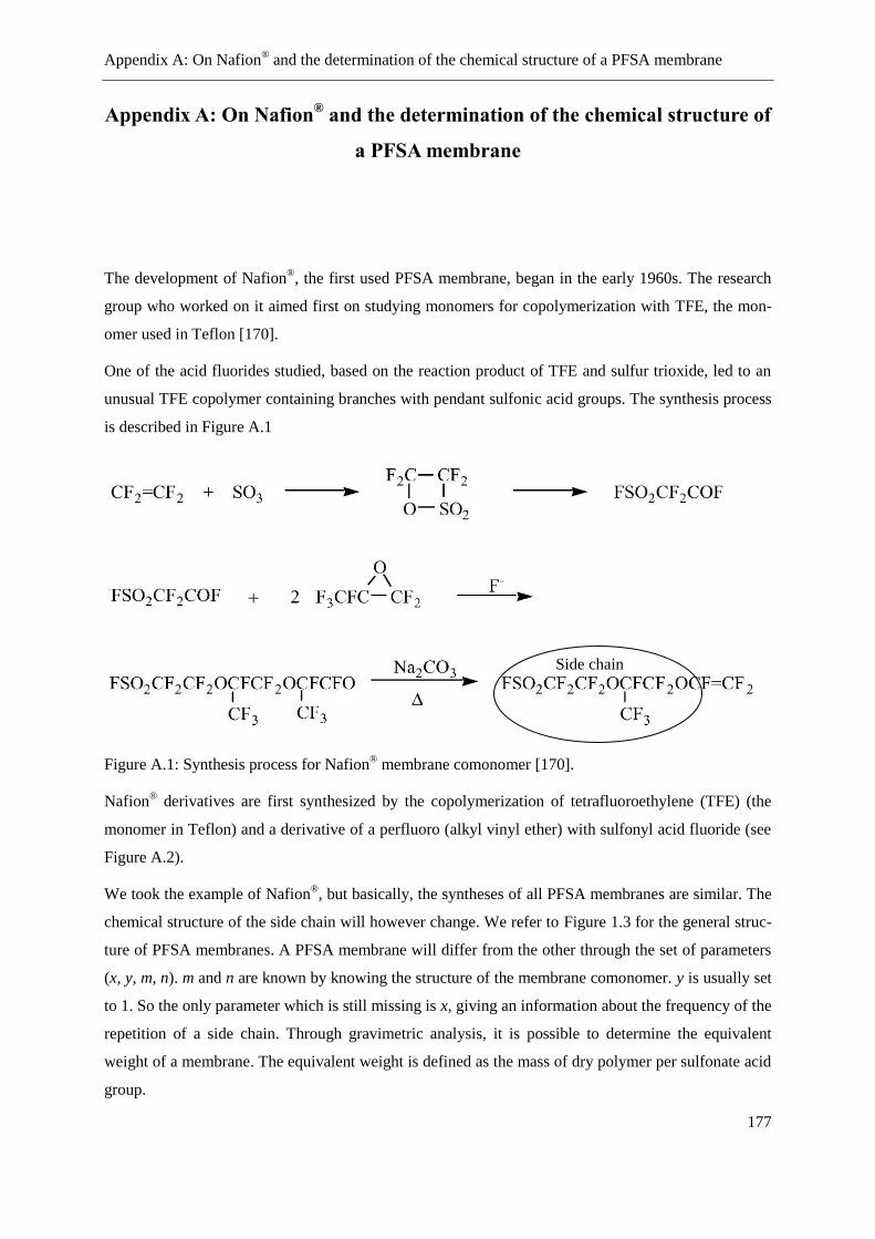
Appendix A: On Nafion® and the determination of the chemical structure of a PFSA membrane
177
Appendix A: On Nafion® and the determination of the chemical structure of
a PFSA membrane
The development of Nafion®, the first used PFSA membrane, began in the early 1960s. The research
group who worked on it aimed first on studying monomers for copolymerization with TFE, the mon-
omer used in Teflon [170].
One of the acid fluorides studied, based on the reaction product of TFE and sulfur trioxide, led to an
unusual TFE copolymer containing branches with pendant sulfonic acid groups. The synthesis process
is described in Figure A.1
Figure A.1: Synthesis process for Nafion® membrane comonomer [170].
Nafion® derivatives are first synthesized by the copolymerization of tetrafluoroethylene (TFE) (the
monomer in Teflon) and a derivative of a perfluoro (alkyl vinyl ether) with sulfonyl acid fluoride (see
Figure A.2).
We took the example of Nafion®, but basically, the syntheses of all PFSA membranes are similar. The
chemical structure of the side chain will however change. We refer to Figure 1.3 for the general struc-
ture of PFSA membranes. A PFSA membrane will differ from the other through the set of parameters
(x, y, m, n). m and n are known by knowing the structure of the membrane comonomer. y is usually set
to 1. So the only parameter which is still missing is x, giving an information about the frequency of the
repetition of a side chain. Through gravimetric analysis, it is possible to determine the equivalent
weight of a membrane. The equivalent weight is defined as the mass of dry polymer per sulfonate acid
group.
Side chain
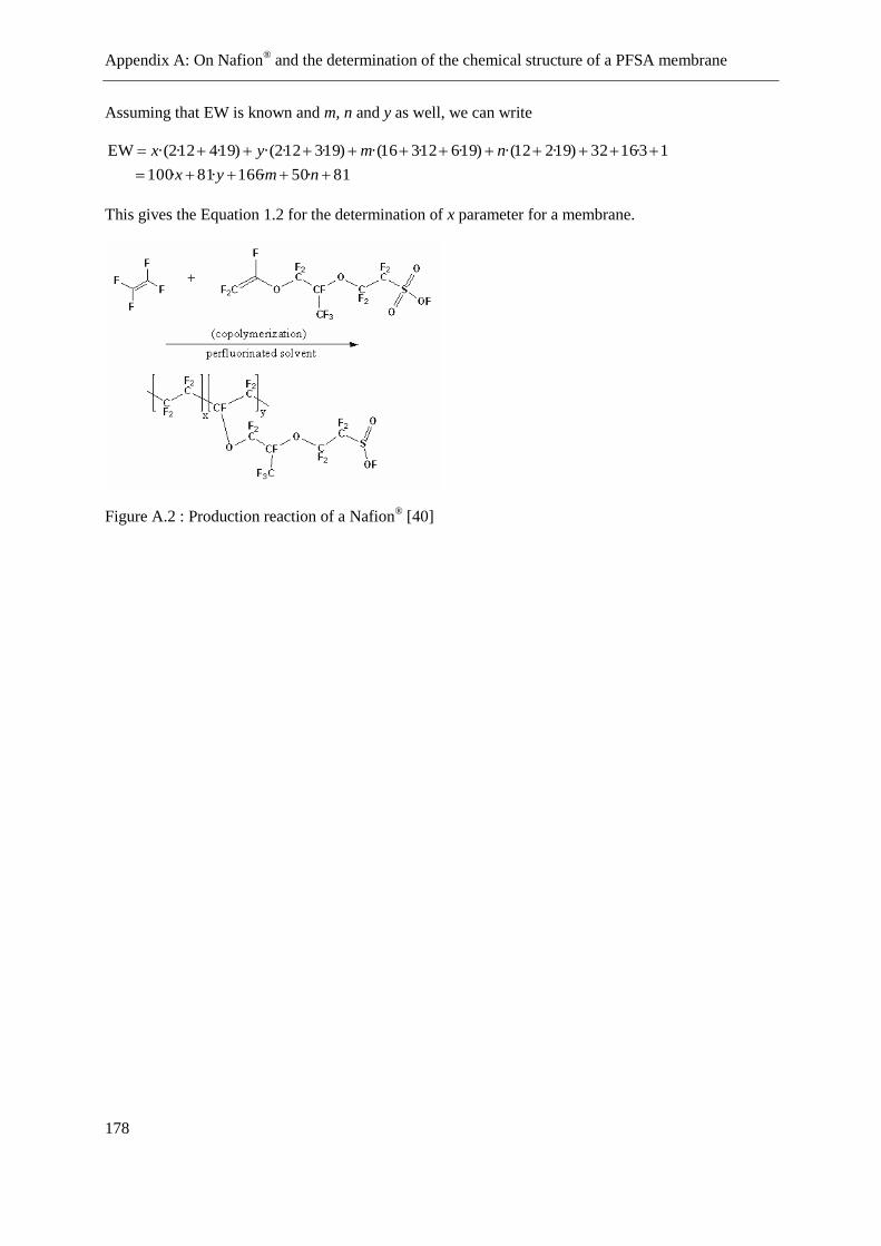
Appendix A: On Nafion® and the determination of the chemical structure of a PFSA membrane
178
Assuming that EW is known and m, n and y as well, we can write
81·50·166·81·100
13·1632)19·212·()19·612·316·()19·312·2·()19·412·2·(EW
nmyx
nmyx
This gives the Equation 1.2 for the determination of x parameter for a membrane.
Figure A.2 : Production reaction of a Nafion® [40]
Appendix B: About Fenton chemistry, its application and its complexity
179
Appendix B: About Fenton chemistry, its application and its complexity
In 1894, Henry Fenton published a work about the oxidation of tartric acid in presence of iron [21].
This was the start of a promising way to treat industrial waste water.
We know under Fenton’s reagent a solution of hydrogen peroxide and iron ions. This reagent is used
to oxidize contaminants or waste water. I can be used for example to oxidize remaining organic com-
pounds from water, especially for waste water of chemical plants. A part of the organic pollution in
such water can be biologically degraded (Biochemical Oxygen Demand) but some refractory organic
pollution can still remain. The addition of Fenton’s reagent in this water will induce the oxidation of
the remaining pollution.
As mentioned in this PhD thesis, the simultaneous presence of hydrogen peroxide and iron ions pro-
duces radicals, one of the most oxidizing species which can be found. These are the responsible of the
degradation of any stable compound in waste water. They are also responsible for the degradation of
PFSA membrane, as discussed earlier.
Test based on Fenton reagents are often used to simulate peroxide attack on PFSA membranes. We
recall the main reaction occurring in the Fenton medium
H2O2 + Fe2+
+ H+ Fe
3+ + HO
· + H2O
However, the mechanism of the Fenton process is far more complex as it is assumed in the previous
reaction. In Figure B.1, a more complete mechanism (in alkaline conditions) is presented with the
corresponding reaction rate constant. As it can be seen, even without the presence of Nafion® in the
system, the possible interaction between iron, hydrogen peroxide and the different products is really
complex. To reproduce faithfully the behavior of all these species in the fuel cell, we decided to keep
some of them. Through this, we ensure that the radicals which are produced during the main reaction
of the Fenton chemistry will not only react with the membrane. This induces a lower attack on the
membrane and more accurate simulations compared to more simple assumptions, like considering
only the disproportionation of hydrogen peroxide.
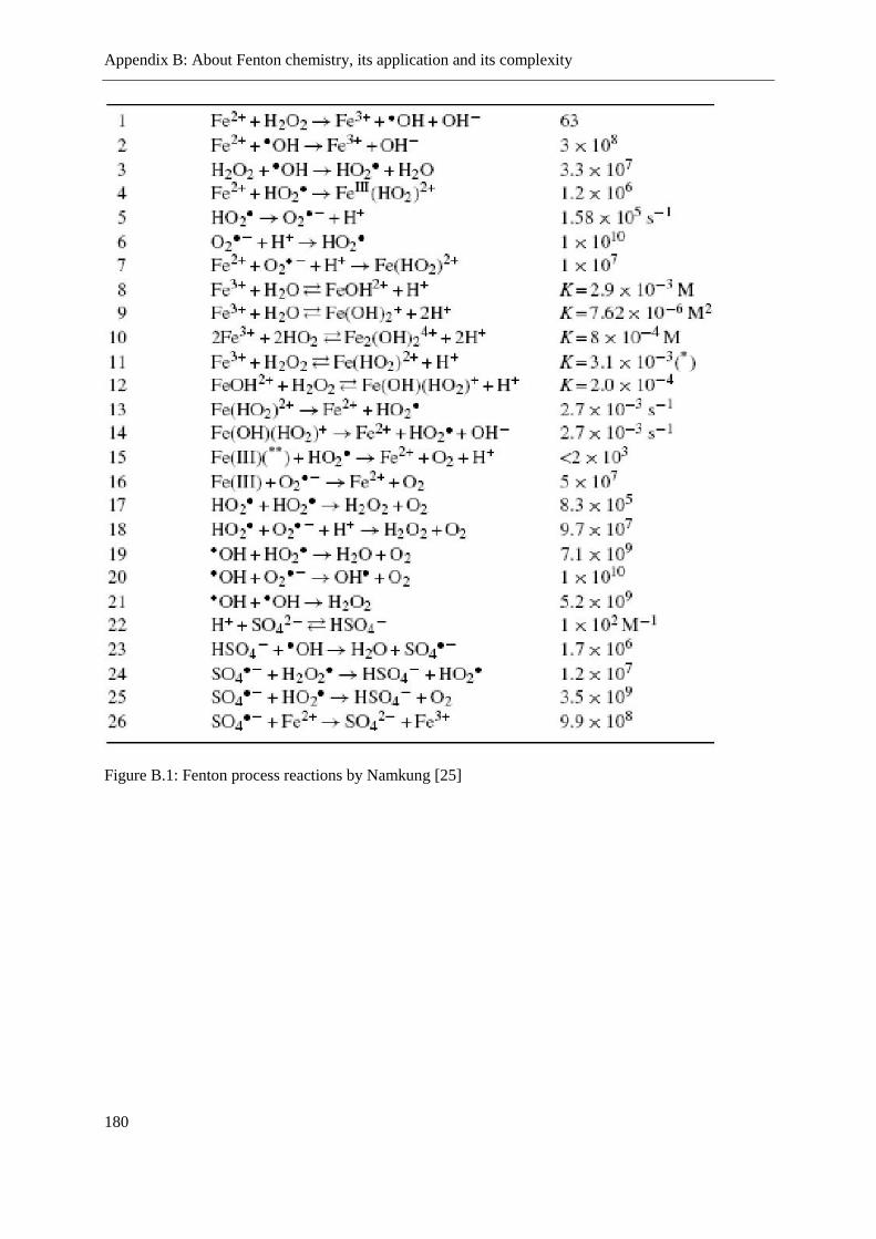
Appendix B: About Fenton chemistry, its application and its complexity
180
Figure B.1: Fenton process reactions by Namkung [25]
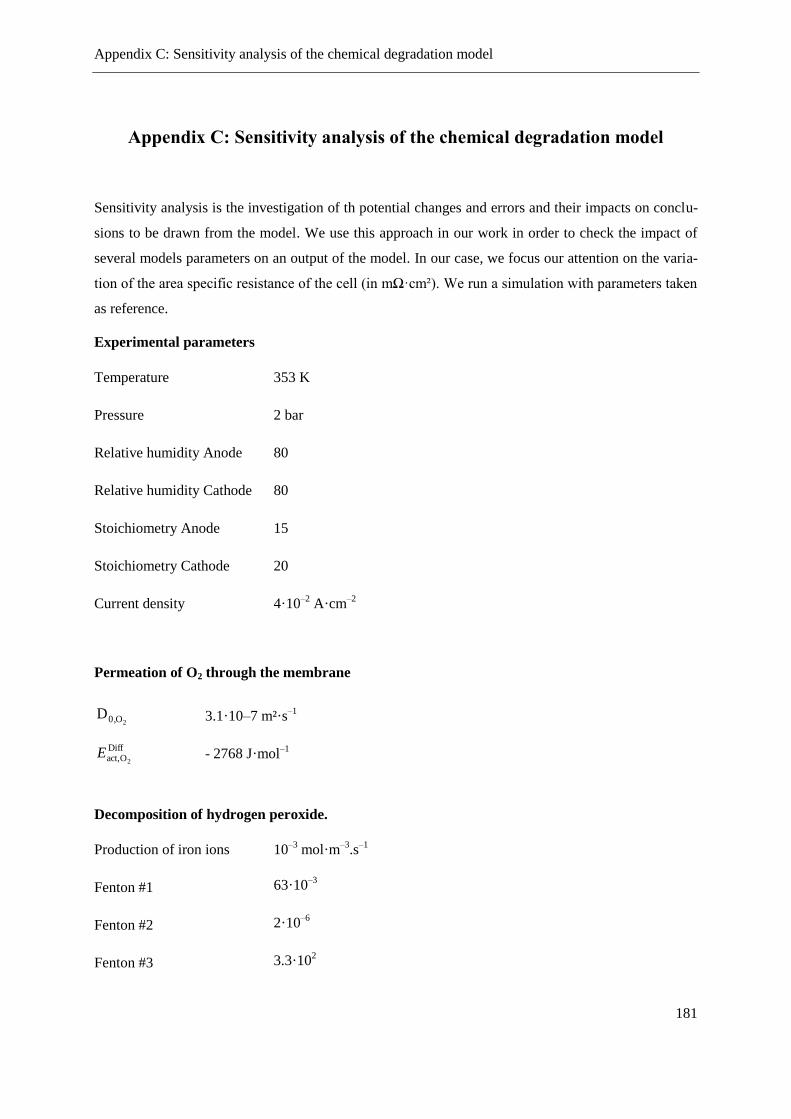
Appendix C: Sensitivity analysis of the chemical degradation model
181
Appendix C: Sensitivity analysis of the chemical degradation model
Sensitivity analysis is the investigation of th potential changes and errors and their impacts on conclu-
sions to be drawn from the model. We use this approach in our work in order to check the impact of
several models parameters on an output of the model. In our case, we focus our attention on the varia-
tion of the area specific resistance of the cell (in mΩ·cm²). We run a simulation with parameters taken
as reference.
Experimental parameters
Temperature 353 K
Pressure 2 bar
Relative humidity Anode 80
Relative humidity Cathode 80
Stoichiometry Anode 15
Stoichiometry Cathode 20
Current density 4·10–2
A·cm–2
Permeation of O2 through the membrane
2O0,D 3.1·10–7 m²·s–1
DiffOact, 2
E - 2768 J·mol–1
Decomposition of hydrogen peroxide.
Production of iron ions 10–3
mol·m–3
.s–1
Fenton #1 63·10–3
Fenton #2 2·10–6
Fenton #3 3.3·102
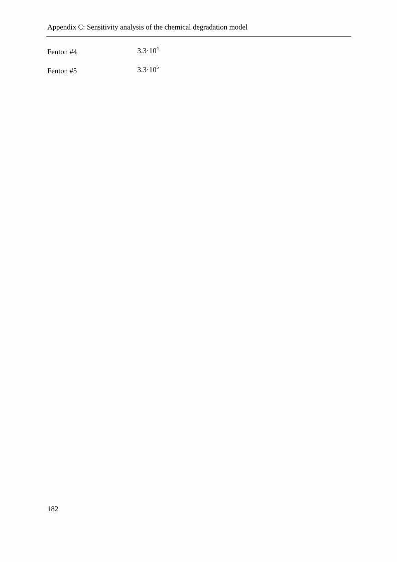
Appendix C: Sensitivity analysis of the chemical degradation model
182
Fenton #4 3.3·104
Fenton #5 3.3·105

Appendix D: Parameters used during the simulations
183
Appendix D: Parameters used during the simulations
Parameters used during the simulations
In our simulations, lot of parameters has been used, and some of them are redundant and not modified
during our investigation on the chemical degradation of the PFSA membrane. In this appendix, these
parameters are given.
Parameters used in Chapter 2:
Parameters used in the transport model
K1 1000 1st acidity constant of sulfuric acid
K2 200 2nd
acidity constant of sulfuric acid
lG 0.255·10–9
m Mean step distance for Grotthus diffusion
lΣ 0.255·10–9
m Mean step distance for surface diffusion
OH2M 18·10
–3 kg·mol
–1 Molar mass of water
Rf 0.254·10–9
m Effective radius of fixed anion groups
Ri 0.143·10–9
m Radius of hydronium ion
Rw 0.141·10–9
m Radius of water molecule
s 0.0122 Swelling coefficient
v 20 number of water molecules surrounding one hydronium
zH+ 1 Charge
αmemb 0.4 Ratio between water flux and effective water flux in the
membrane
βmemb 8.5 mol·m–2
·s–1
Proportionality coefficient between water flux into the
membrane and water content difference over electrode /
membrane interface
δ 0.143·10–9
m Distance between proton in hydronium ion an proton-
accepting water molecule
εr 6 Relative permittivity of the membrane

Appendix D: Parameters used during the simulations
184
η 0.000355 Pa·–1
Viscosity of water
θF π/12 Final angle diffusing proton and an adjacent water mole-
cule
θI π·107/180 Initial angle between diffusing proton and adjacent water
molecule
μW 0.61·10–29
C·m–1
Dipole moment of liquid water
Henry’s constants, diffusion coefficients and related activation energies for the motion of species in
the membrane
2O0,H 12.8·10–6
mol·m–3
·Pa–1
Henry
Oact, 2E – 10808 J·mol
–1
2H0,H 7.6·10–6
mol·m–3
·Pa–1
Henry
Oact, 2E – 4157 J·mol
–1
2O0,D 3.1·10–7
m²·s–1
DiffOact, 2
E – 2768 J·mol–1
2H0,D 4.1·10–10
m²·s–1
DiffHact, 2
E – 2602 J·mol–1
iD0, 10–7
m²·s–1
(default values for all the others species)
Diffiact,E 0 J·mol
–1(default values for all the others species)
Fenton’s reaction rate constant
Reaction 2.1 63·10–3
m3·mol
–1·s
–1
Reaction 2.2 2·10–6
·mol–1
·s–1
Reaction 2.3 3.3·102·mol
–1·s
–1
Reaction 2.4 3.3·104·mol
–1·s
–1
Reaction 2.5 3.3·105·mol
–1·s
–1

Appendix D: Parameters used during the simulations
185
Parameters used in Chapter 3:
01,cG 1000 J·mol
–1
02,cG 1000 J·mol
–1
d 2·10–10
εCL,anode 6·ε0
εCL,cathode 4·ε0
εDL 20·ε0


References
187
References
[1] D.M. Bernardi, M.W. Verbrugge, "A Mathematical Model of the Solid-Polymer-Electrolyte Fuel
Cell", Journal of The Electrochemical Society, 139 (1992) 2477-2491.
[2] A.A. Franco, PEMFC degradation modeling and analysis, in: C. Hartnig, C. Roth (Eds.) Polymer
electrolyte membrane and direct methanol fuel cell technology (PEMFCs and DMFCs), Woodhead,
Cambridge, UK, 2011.
[3] A.A. Franco, M. Gerard, "Multiscale Model of Carbon Corrosion in a PEFC: Coupling with
Electrocatalysis and Impact on Performance Degradation", Journal of The Electrochemical Society,
155 (2008) B367-B384.
[4] A.A. Franco, S. Passot, P. Fugier, C. Anglade, E. Billy, L. Guetaz, N. Guillet, E. De Vito, S.
Mailley, "PtxCoy Catalysts Degradation in PEFC Environments: Mechanistic Insights", Journal of The
Electrochemical Society, 156 (2009) B410-B424.
[5] A.A. Franco, M. Tembely, "Transient Multiscale Modeling of Aging Mechanisms in a PEFC
Cathode", Journal of The Electrochemical Society, 154 (2007) B712-B723.
[6] Scientific modelling, http://en.wikipedia.org/wiki/Scientific_modelling
[7] A.A. Franco, PEMFC degradation modeling an analysis, in: C. Hartnig, C. Roth (Eds.) Polymer
electrolyte membrane and direct methanol fuel cell technology, vol. 1, Woodhead, Cambridge, UK,
2011.
[8] A.A. Franco, M. Guinard, B. Barthe, O. Lemaire, "Impact of carbon monoxide on PEFC catalyst
carbon support degradation under current-cycled operating conditions", Electrochimica Acta, 54
(2009) 5267-5279.
[9] K. Malek, A.A. Franco, "Microstructure-Based Modeling of Aging Mechanisms in Catalyst Layers
of Polymer Electrolyte Fuel Cells", The Journal of Physical Chemistry B, 115 (2011) 8088-8101.
[10] T.D. Gierke, G.E. Munn, F.C. Wilson, "The morphology in nafion perfluorinated membrane
products, as determined by wide- and small-angle x-ray studies", Journal of Polymer Science:
Polymer Physics Edition, 19 (1981) 1687-1704.
[11] H.G. Haubold, T. Vad, H. Jungbluth, P. Hiller, "Nano structure of NAFION: a SAXS study",
Electrochimica Acta, 46 (2001) 1559-1563.
[12] L. Rubatat, A.L. Rollet, G. Gebel, O. Diat, "Evidence of Elongated Polymeric Aggregates in
Nafion", Macromolecules, 35 (2002) 4050-4055.
[13] K. Schmidt-Rohr, Q. Chen, "Parallel cylindrical water nanochannels in Nafion fuel-cell
membranes", Nat Mater, 7 (2008) 75-83.
[14] H.L. Yeager, A. Steck, "Cation and Water Diffusion in Nafion Ion Exchange Membranes:
Influence of Polymer Structure", Journal of The Electrochemical Society, 128 (1981) 1880-1884.
[15] J. Healy, C. Hayden, T. Xie, K. Olson, R. Waldo, M. Brundage, H. Gasteiger, J. Abbott, "Aspects

References
188
of the Chemical Degradation of PFSA Ionomers used in PEM Fuel Cells", Fuel Cells, 5 (2005) 302-
308.
[16] A.P. Young, J. Stumper, S. Knights, E. Gyenge, "Ionomer Degradation in Polymer Electrolyte
Membrane Fuel Cells", Journal of The Electrochemical Society, 157 (2010) B425-B436.
[17] O. Antoine, R. Durand, "RRDE study of oxygen reduction on Pt nanoparticles inside Nafion®:
H2O2 production in PEMFC cathode conditions", Journal of Applied Electrochemistry, 30 (2000)
839-844.
[18] W. Liu, D. Zuckerbrod, "In Situ Detection of Hydrogen Peroxide in PEM Fuel Cells", Journal of
The Electrochemical Society, 152 (2005) A1165-A1170.
[19] V.A. Sethuraman, J.W. Weidner, A.T. Haug, S. Motupally, L.V. Protsailo, "Hydrogen Peroxide
Formation Rates in a PEMFC Anode and Cathode", Journal of The Electrochemical Society, 155
(2008) B50-B57.
[20] R. Andreozzi, A. D'Apuzzo, R. Marotta, "A kinetic model for the degradation of benzothiazole by
Fe3+
-photo-assisted Fenton process in a completely mixed batch reactor", J. Hazard. Mater., B80
(2000) 17.
[21] H.J.H. Fenton, "LXXIII.-Oxidation of tartaric acid in presence of iron", Journal of the Chemical
Society, Transactions, 65 (1894) 899-910.
[22] W. Gernjak, T. Krutzler, A. Glaser, S. Malato, J. Caceres, R. Bauer, A.R. Fernández-Alba,
"Photo-Fenton treatment of water containing natural phenolic pollutants", Chemosphere, 50 (2003)
71-78.
[23] P.L. Huston, J.J. Pignatello, "Degradation of selected pesticide active ingredients and
commercial formulations in water by the photo-assisted Fenton reaction", Water Research, 33 (1999)
1238-1246.
[24] J. Kiwi, C. Pulgarin, P. Peringer, "Effect of Fenton and photo-Fenton reactions on the
degradation and biodegradability of 2 and 4-nitrophenols in water treatment", Applied Catalysis B:
Environmental, 3 (1994) 335-350.
[25] K.C. Namkung, P. Sharratt, "Fenton and Photo-Fenton Processes for Treatment of Aqueous
Wastes", UMIST.
[26] C.C. Winterbourn, "Toxicity of iron and hydrogen peroxide: the Fenton reaction", Toxicol. Lett.,
82/83 (1995) 6.
[27] M. Danilczuk, F.D. Coms, S. Schlick, "Visualizing Chemical Reactions and Crossover Processes
in a Fuel Cell Inserted in the ESR Resonator: Detection by Spin Trapping of Oxygen Radicals, Nafion-
Derived Fragments, and Hydrogen and Deuterium Atoms", The Journal of Physical Chemistry B, 113
(2009) 8031-8042.
[28] M.K. Kadirov, A. Bosnjakovic, S. Schlick, "Membrane-Derived Fluorinated Radicals Detected
by Electron Spin Resonance in UV-Irradiated Nafion and Dow Ionomers: Effect of Counterions and
References
189
H2O2", The Journal of Physical Chemistry B, 109 (2005) 7664-7670.
[29] M. Kitazawa, A. Nosaka, Y. Nosaka, "Radical formation in polymer electrolyte fuel cell
components as studied by ESR spectroscopy", Journal of Applied Electrochemistry, 38 (2008) 491-
496.
[30] A. Panchenko, H. Dilger, J. Kerres, M. Hein, A. Ullrich, T. Kaz, E. Roduner, "In-situ spin trap
electron paramagnetic resonance study of fuel cell processes", Physical Chemistry Chemical Physics,
6 (2004) 2891-2894.
[31] D.A. Schiraldi, "Perfluorinated Polymer Electrolyte Membrane Durability", Journal of
Macromolecular Science, Part C: Polymer Reviews, 46 (2006) 315-327.
[32] T. Xie, C.A. Hayden, "A kinetic model for the chemical degradation of perfluorinated sulfonic
acid ionomers: Weak end groups versus side chain cleavage", Polymer, 48 (2007) 5497-5506.
[33] C. Chen, T. Fuller, "H2O2 Formation under Fuel-Cell Conditions", ECS Transactions, 11 (2007)
1127-1137.
[34] C. Chen, T.F. Fuller, "The effect of humidity on the degradation of Nafion® membrane", Polymer
Degradation and Stability, 94 (2009) 1436-1447.
[35] C. Chen, T.F. Fuller, "XPS Analysis of Polymer Membrane Degradation in PEMFCs", Journal of
The Electrochemical Society, 156 (2009) B1218-B1224.
[36] C. Chen, T.F. Fuller, "Modeling of H2O2 formation in PEMFCs", Electrochimica Acta, 54 (2009)
3984-3995.
[37] C. Chen, G. Levitin, D.W. Hess, T.F. Fuller, "XPS investigation of Nafion membrane
degradation", Journal of Power Sources, 169 (2007) 288-295.
[38] L. Gubler, S.M. Dockheer, W.H. Koppenol, "Radical (HO·, H· and HOO·) Formation and
Ionomer Degradation in Polymer Electrolyte Fuel Cells", Journal of The Electrochemical Society, 158
(2011) B755-B769.
[39] A.A. Shah, T.R. Ralph, F.C. Walsh, "Modeling and Simulation of the Degradation of
Perfluorinated Ion-Exchange Membranes in PEM Fuel Cells", Journal of The Electrochemical
Society, 156 (2009) B465-B484.
[40] http://en.wikipedia.org/wiki/Henry%27s_law
[41] F. Fouda-Onana, N. Guillet, Method for depositing a metal onto a porous carbon layer, in, France,
2009.
[42] H. Pu, W.H. Meyer, G. Wegner, "Proton transport in polybenzimidazole blended with H3PO4 or
H2SO4", Journal of Polymer Science Part B: Polymer Physics, 40 (2002) 663-669.
[43] S.J. Paddison, T.A. Zawodzinski Jr, "Molecular modeling of the pendant chain in Nafion", Solid
State Ionics, 113-115 (1998) 333-340.
[44] A. Vishnyakov, A.V. Neimark, "Molecular Simulation Study of Nafion Membrane Solvation in
Water and Methanol", The Journal of Physical Chemistry B, 104 (2000) 4471-4478.

References
190
[45] K. Malek, M. Eikerling, Q. Wang, T. Navessin, Z. Liu, "Self-Organization in Catalyst Layers of
Polymer Electrolyte Fuel Cells", The Journal of Physical Chemistry C, 111 (2007) 13627-13634.
[46] S. Schlick, G. Gebel, M. Pineri, F. Volino, "Fluorine-19 NMR spectroscopy of acid Nafion
membranes and solutions", Macromolecules, 24 (1991) 3517-3521.
[47] N.G. Boyle, V.J. McBrierty, A. Eisenberg, "NMR investigation of molecular motion in Nafion
membranes", Macromolecules, 16 (1983) 80-84.
[48] Q. Chen, K. Schmidt-Rohr, "19
F and 13
C NMR Signal Assignment and Analysis in a
Perfluorinated Ionomer (Nafion) by Two-Dimensional Solid-State NMR", Macromolecules, 37 (2004)
5995-6003.
[49] Q. Chen, K. Schmidt-Rohr, "Backbone Dynamics of the Nafion Ionomer Studied by 19
F-13
C Solid-
State NMR", Macromolecular Chemistry and Physics, 208 (2007) 2189-2203.
[50] J.A. Elliott, D. Wu, S.J. Paddison, R.B. Moore, "A unified morphological description of Nafion
membranes from SAXS and mesoscale simulations", Soft Matter, (2011).
[51] G. Gebel, O. Diat, "Neutron and X-ray Scattering: Suitable Tools for Studying Ionomer
Membranes", Fuel Cells, 5 (2005) 261-276.
[52] J. Halim, F.N. Büchi, O. Haas, M. Stamm, G.G. Scherer, "Characterization of perfluorosulfonic
acid membranes by conductivity measurements and small-angle x-ray scattering", Electrochimica
Acta, 39 (1994) 1303-1307.
[53] K.A. Page, F.A. Landis, A.K. Phillips, R.B. Moore, "SAXS Analysis of the Thermal Relaxation of
Anisotropic Morphologies in Oriented Nafion Membranes", Macromolecules, 39 (2006) 3939-3946.
[54] E.J. Roche, M. Pineri, R. Duplessix, A.M. Levelut, "Small-angle scattering studies of nafion
membranes", Journal of Polymer Science: Polymer Physics Edition, 19 (1981) 1-11.
[55] A. Eisenberg, B. Hird, R.B. Moore, "A new multiplet-cluster model for the morphology of random
ionomers", Macromolecules, 23 (1990) 4098-4107.
[56] W.Y. Hsu, T.D. Gierke, "Elastic theory for ionic clustering in perfluorinated ionomers",
Macromolecules, 15 (1982) 101-105.
[57] W.Y. Hsu, T.D. Gierke, "Ion transport and clustering in nafion perfluorinated membranes",
Journal of Membrane Science, 13 (1983) 307-326.
[58] K.A. Mauritz, R.B. Moore, "State of Understanding of Nafion", Chemical Reviews, 104 (2004)
4535-4586.
[59] D. Gierke T, Y. Hsu W, The Cluster-Network Model of Ion Clustering in Perfluorosulfonated
Membranes, in: Perfluorinated Ionomer Membranes, vol. 180, AMERICAN CHEMICAL SOCIETY,
1982, pp. 283-307.
[60] M. Fujimura, T. Hashimoto, H. Kawai, "Small-angle x-ray scattering study of perfluorinated
ionomer membranes. 1. Origin of two scattering maxima", Macromolecules, 14 (1981) 1309-1315.
[61] M. Fujimura, T. Hashimoto, H. Kawai, "Small-angle x-ray scattering study of perfluorinated

References
191
ionomer membranes. 2. Models for ionic scattering maximum", Macromolecules, 15 (1982) 136-144.
[62] M.H. Litt, Proc. 1997 ACS San Francisco Meeting, San Francisco, 1997.
[63] G. Gebel, "Structural evolution of water swollen perfluorosulfonated ionomers from dry
membrane to solution", Polymer, 41 (2000) 5829-5838.
[64] Z. Siroma, N. Fujiwara, T. Ioroi, S. Yamazaki, K. Yasuda, Y. Miyazaki, "Dissolution of Nafion
membrane and recast Nafion film in mixtures of methanol and water", Journal of Power Sources, 126
(2004) 41-45.
[65] L. Rubatat, G. Gebel, O. Diat, "Fibrillar Structure of Nafion: Matching Fourier and Real Space
Studies of Corresponding Films and Solutions", Macromolecules, 37 (2004) 7772-7783.
[66] A.Z. Weber, J. Newman, "Transport in Polymer-Electrolyte Membranes", Journal of The
Electrochemical Society, 150 (2003) A1008-A1015.
[67] A.Z. Weber, J. Newman, "Transport in Polymer-Electrolyte Membranes", Journal of The
Electrochemical Society, 151 (2004) A311-A325.
[68] B. Chu, C. Wu, W. Buck, "Light-scattering characterization of poly(tetrafluoroethylene). 2.
PTFE in perfluorotetracosane: molecular weight distribution and solution properties",
Macromolecules, 22 (1989) 831-837.
[69] B. Rosi-Schwartz, G.R. Mitchell, "Extracting force fields for disordered polymeric materials
from neutron scattering data", Polymer, 37 (1996) 1857-1870.
[70] R. Borup, J. Meyers, B. Pivovar, Y.S. Kim, R. Mukundan, N. Garland, D. Myers, M. Wilson, F.
Garzon, D. Wood, P. Zelenay, K. More, K. Stroh, T. Zawodzinski, J. Boncella, J.E. McGrath, M.
Inaba, K. Miyatake, M. Hori, K. Ota, Z. Ogumi, S. Miyata, A. Nishikata, Z. Siroma, Y. Uchimoto, K.
Yasuda, K.-i. Kimijima, N. Iwashita, "Scientific Aspects of Polymer Electrolyte Fuel Cell Durability
and Degradation", Chemical Reviews, 107 (2007) 3904-3951.
[71] H. Tang, S. Peikang, S.P. Jiang, F. Wang, M. Pan, "A degradation study of Nafion proton
exchange membrane of PEM fuel cells", Journal of Power Sources, 170 (2007) 85-92.
[72] M. Inaba, T. Kinumoto, M. Kiriake, R. Umebayashi, A. Tasaka, Z. Ogumi, "Gas crossover and
membrane degradation in polymer electrolyte fuel cells", Electrochimica Acta, 51 (2006) 5746-5753.
[73] M. Schulze, N. Wagner, T. Kaz, K.A. Friedrich, "Combined electrochemical and surface analysis
investigation of degradation processes in polymer electrolyte membrane fuel cells", Electrochimica
Acta, 52 (2007) 2328-2336.
[74] S. Zhang, X.-Z. Yuan, J.N.C. Hin, H. Wang, K.A. Friedrich, M. Schulze, "A review of platinum-
based catalyst layer degradation in proton exchange membrane fuel cells", Journal of Power Sources,
194 (2009) 588-600.
[75] S.S. Kocha, J. Deliang Yang, J.S. Yi, "Characterization of gas crossover and its implications in
PEM fuel cells", AIChE Journal, 52 (2006) 1916-1925.
[76] E.H. Jung, U.H. Jung, T.H. Yang, D.H. Peak, D.H. Jung, S.H. Kim, "Methanol crossover through
References
192
PtRu/Nafion composite membrane for a direct methanol fuel cell", International Journal of Hydrogen
Energy, 32 (2007) 903-907.
[77] A.C. Fernandes, E.A. Ticianelli, "A performance and degradation study of Nafion 212 membrane
for proton exchange membrane fuel cells", Journal of Power Sources, 193 (2009) 547-554.
[78] V.O. Mittal, H.R. Kunz, J.M. Fenton, "Is H2O2 Involved in the Membrane Degradation
Mechanism in PEMFC?", Electrochemical and Solid-State Letters, 9 (2006) A299-A302.
[79] M.O. Davies, M. Clark, E. Yeager, F. Hovorka, "The Oxygen Electrode", Journal of The
Electrochemical Society, 106 (1959) 56-61.
[80] E. Yeager, "Dioxygen electrocatalysis: mechanisms in relation to catalyst structure", Journal of
Molecular Catalysis, 38 (1986) 5-25.
[81] I. Morcos, E. Yeager, "Kinetic studies of the oxygen--peroxide couple on pyrolytic graphite",
Electrochimica Acta, 15 (1970) 953-975.
[82] E. Yeager, "Electrocatalysts for O2 reduction", Electrochimica Acta, 29 (1984) 1527-1537.
[83] E. Yeager, P. Krouse, K.V. Rao, "The kinetics of the oxygen--peroxide couple on carbon",
Electrochimica Acta, 9 (1964) 1057-1070.
[84] R. Ferreira de Morais, A.A. Franco, P. Sautet, D. Loffreda, "Water vs Hydrogen Peroxide
Formation on Pt(111) From a First-Principles Study. 2. Coverage Kinetics", (in preparation).
[85] R. Ferreira de Morais, P. Sautet, D. Loffreda, A.A. Franco, "A multiscale theoretical methodology
for the calculation of electrochemical observables from ab initio data: Application to the oxygen
reduction reaction in a Pt(111)-based polymer electrolyte membrane fuel cell", Electrochimica Acta,
In Press, Corrected Proof (2011).
[86] V.R. Stamenkovic, B. Fowler, B.S. Mun, G. Wang, P.N. Ross, C.A. Lucas, N.M. Marković,
"Improved Oxygen Reduction Activity on Pt3Ni(111) via Increased Surface Site Availability", Science,
315 (2007) 493-497.
[87] Y. Wang, P.B. Balbuena, "Ab Initio Molecular Dynamics Simulations of the Oxygen Reduction
Reaction on a Pt(111) Surface in the Presence of Hydrated Hydronium (H3O)+(H2O)2: Direct or
Series Pathway?", The Journal of Physical Chemistry B, 109 (2005) 14896-14907.
[88] Y. Wang, P.B. Balbuena, "Potential Energy Surface Profile of the Oxygen Reduction Reaction on
a Pt Cluster: Adsorption and Decomposition of OOH and H2O2", Journal of Chemical Theory and
Computation, 1 (2005) 935-943.
[89] A. Pozio, R.F. Silva, M. De Francesco, L. Giorgi, "Nafion degradation in PEFCs from end plate
iron contamination", Electrochimica Acta, 48 (2003) 1543-1549.
[90] F.N. Büchi, M. Inaba, T.J. Schmidt, J. Scherer, D. Münter, R. Ströbel, Influence of Metallic
Bipolar Plates on the Durability of Polymer Electrolyte Fuel Cells, in: Polymer Electrolyte Fuel Cell
Durability, Springer New York, 2009, pp. 243-255.
[91] M. Aoki, H. Uchida, M. Watanabe, "Decomposition mechanism of perfluorosulfonic acid

References
193
electrolyte in polymer electrolyte fuel cells", Electrochemistry Communications, 8 (2006) 1509-1513.
[92] A. Panchenko, H. Dilger, E. Möller, T. Sixt, E. Roduner, "In situ EPR investigation of polymer
electrolyte membrane degradation in fuel cell applications", Journal of Power Sources, 127 (2004)
325-330.
[93] B. Vogel, E. Aleksandrova, S. Mitov, M. Krafft, A. Dreizler, J. Kerres, M. Hein, E. Roduner,
"Observation of Fuel Cell Membrane Degradation by Ex Situ and In Situ Electron Paramagnetic
Resonance", Journal of The Electrochemical Society, 155 (2008) B570-B574.
[94] H. Liu, H.A. Gasteiger, A. Laconti, J. Zhang, "Factors Impacting Chemical Degradation Of
Perfluorinated Sulfonic Acid Ionomers", ECS Transactions, 1 (2006) 283-293.
[95] F.N. Büchi, M. Inaba, T.J. Schmidt, M. Inaba, Chemical Degradation of Perfluorinated Sulfonic
Acid Membranes, in: Polymer Electrolyte Fuel Cell Durability, Springer New York, 2009, pp. 57-69.
[96] F.N. Büchi, M. Inaba, T.J. Schmidt, H. Liu, F.D. Coms, J. Zhang, H.A. Gasteiger, A.B. LaConti,
Chemical Degradation: Correlations Between Electrolyzer and Fuel Cell Findings, in: Polymer
Electrolyte Fuel Cell Durability, Springer New York, 2009, pp. 71-118.
[97] T. Kinumoto, M. Inaba, Y. Nakayama, K. Ogata, R. Umebayashi, A. Tasaka, Y. Iriyama, T. Abe,
Z. Ogumi, "Durability of perfluorinated ionomer membrane against hydrogen peroxide", Journal of
Power Sources, 158 (2006) 1222-1228.
[98] S. Kundu, M.W. Fowler, L.C. Simon, R. Abouatallah, N. Beydokhti, "Open circuit voltage
durability study and model of catalyst coated membranes at different humidification levels", Journal of
Power Sources, 195 (2010) 7323-7331.
[99] T. Madden, D. Weiss, N. Cipollini, D. Condit, M. Gummalla, S. Burlatsky, V. Atrazhev,
"Degradation of Polymer-Electrolyte Membranes in Fuel Cells", Journal of The Electrochemical
Society, 156 (2009) B657-B662.
[100] S. Kundu, L.C. Simon, M.W. Fowler, "Comparison of two accelerated Nafion degradation
experiments", Polymer Degradation and Stability, 93 (2008) 214-224.
[101] T. Ishimoto, R. Nagumo, T. Ogura, T. Ishihara, B. Kim, A. Miyamoto, M. Koyama, "Chemical
Degradation Mechanism of Model Compound, CF3(CF2)3O(CF2)2OCF2SO3H, of PFSA Polymer by
Attack of Hydroxyl Radical in PEMFCs", Journal of The Electrochemical Society, 157 (2010) B1305-
B1309.
[102] S.M. Dockheer, L. Gubler, P.L. Bounds, A.S. Domazou, G.G. Scherer, A. Wokaun, W.H.
Koppenol, "Damage to fuel cell membranes. Reaction of HO· with an oligomer of poly(sodium styrene
sulfonate) and subsequent reaction with O2", Physical Chemistry Chemical Physics, 12 (2010) 11609-
11616.
[103] M.W. Fowler, R.F. Mann, J.C. Amphlett, B.A. Peppley, P.R. Roberge, "Incorporation of voltage
degradation into a generalised steady state electrochemical model for a PEM fuel cell", Journal of
Power Sources, 106 (2002) 274-283.

References
194
[104] G.V. Buxton, L. Clive, W. Greenstock, P. Helman, A.B. Ross, "Critical review of rate constants
for reactions of hydrated electrons, hydrogen atoms and hydroxyl radicals in aqueous solution", J.
Phys. Chem. Ref. Data, 17 (1988) 513-886.
[105] H. Christensen, K. Sehested, H. Corfitzen, "Reactions of hydroxyl radicals with hydrogen
peroxide at ambient and elevated temperatures", The Journal of Physical Chemistry, 86 (1982) 1588-
1590.
[106] J. De Laat, H. Gallard, "Catalytic Decomposition of Hydrogen Peroxide by Fe(III) in
Homogeneous Aqueous Solution: Mechanism and Kinetic Modeling", Environmental Science &
Technology, 33 (1999) 2726-2732.
[107] F. Haber, J. Weiss, The Catalytic Decomposition of Hydrogen Peroxide by Iron Salts, in, 1934,
pp. 332-351.
[108] S.-S. Lin, M.D. Gurol, "Catalytic Decomposition of Hydrogen Peroxide on Iron Oxide: Kinetics,
Mechanism, and Implications", Environmental Science & Technology, 32 (1998) 1417-1423.
[109] T.E. Springer, T.A. Zawodzinski, S. Gottesfeld, "Polymer Electrolyte Fuel Cell Model", Journal
of The Electrochemical Society, 138 (1991) 2334-2342.
[110] M. Eikerling, Y.I. Kharkats, A.A. Kornyshev, Y.M. Volfkovich, "Phenomenological Theory of
Electro-osmotic Effect and Water Management in Polymer Electrolyte Proton-Conducting
Membranes", Journal of The Electrochemical Society, 145 (1998) 2684-2699.
[111] W. Weppner, R.A. Huggins, "Determination of the Kinetic Parameters of Mixed-Conducting
Electrodes and Application to the System Li[sub 3]Sb", Journal of The Electrochemical Society, 124
(1977) 1569-1578.
[112] S. Motupally, A.J. Becker, J.W. Weidner, "Diffusion of Water in Nafion 115 Membranes",
Journal of The Electrochemical Society, 147 (2000) 3171-3177.
[113] T.A. Zawodzinski, M. Neeman, L.O. Sillerud, S. Gottesfeld, "Determination of water diffusion
coefficients in perfluorosulfonate ionomeric membranes", The Journal of Physical Chemistry, 95
(1991) 6040-6044.
[114] T.V. Nguyen, R.E. White, "A Water and Heat Management Model for Proton-Exchange-
Membrane Fuel Cells", Journal of The Electrochemical Society, 140 (1993) 2178-2186.
[115] M. Ise, K.D. Kreuer, J. Maier, "Electroosmotic drag in polymer electrolyte membranes: an
electrophoretic NMR study", Solid State Ionics, 125 (1999) 213-223.
[116] T.A. Zawodzinski, J. Davey, J. Valerio, S. Gottesfeld, "The water content dependence of
electro-osmotic drag in proton-conducting polymer electrolytes", Electrochimica Acta, 40 (1995) 297-
302.
[117] S. Ge, B. Yi, P. Ming, "Experimental Determination of Electro-Osmotic Drag Coefficient in
Nafion Membrane for Fuel Cells", Journal of The Electrochemical Society, 153 (2006) A1443-A1450.
[118] T.F. Fuller, J. Newman, "Experimental Determination of the Transport Number of Water in

References
195
Nafion 117 Membrane", Journal of The Electrochemical Society, 139 (1992) 1332-1337.
[119] C. Vallieres, D. Winkelmann, D. Roizard, E. Favre, P. Scharfer, M. Kind, "On Schroeder's
paradox", Journal of Membrane Science, 278 (2006) 357-364.
[120] M.H. Eikerling, P. Berg, "Poroelectroelastic theory of water sorption and swelling in polymer
electrolyte membranes", Soft Matter, 7 (2011) 5976-5990.
[121] M. Holz, "Electrophoretic NMR", Chemical Society Reviews, 23 (1994) 165-174.
[122] F. Meier, G. Eigenberger, "Transport parameters for the modelling of water transport in
ionomer membranes for PEM-fuel cells", Electrochimica Acta, 49 (2004) 1731-1742.
[123] A. Ohma, S. Yamamoto, K. Shinohara, "Membrane degradation mechanism during open-circuit
voltage hold test", Journal of Power Sources, 182 (2008) 39-47.
[124] K. Hongsirikarn, X. Mo, J.G. Goodwin Jr, S. Creager, "Effect of H2O2 on Nafion properties and
conductivity at fuel cell conditions", Journal of Power Sources, 196 (2010) 3060-3072.
[125] M. Aoki, H. Uchida, M. Watanabe, "Novel evaluation method for degradation rate of polymer
electrolytes in fuel cells", Electrochemistry Communications, 7 (2005) 1434-1438.
[126] E.T. Denisov, T.G. Denisova, T.S. Pokidova, Handbook of Free Radical Initiators, in:
Handbook of Free Radical Initiators, John Wiley & Sons, Inc., 2005, pp. i-xxii.
[127] F. Haber, J. Weiss, "Über die Katalyse des Hydroperoxydes", Naturwissenschaften, 20 (1932)
948-950.
[128] S. Prager, "Diffusion in Inhomogeneous Media", Journal of Chemical Physics, 33 (1960) 122-
127.
[129] H. Yasuda, C.E. Lamaze, L.D. Ikenberry, "Permeability of solutes through hydrated polymer
membranes. Part I. Diffusion of sodium chloride", Die Makromolekulare Chemie, 118 (1968) 19-35.
[130] S. Koter, "Transport of simple electrolyte solutions through ion-exchange membranes--the
capillary model", Journal of Membrane Science, 206 (2002) 201-215.
[131] P. Choi, N.H. Jalani, R. Datta, "Thermodynamics and Proton Transport in Nafion", Journal of
The Electrochemical Society, 152 (2005) E123-E130.
[132] A.A. Franco, Un modèle physique multiéchelle de la dynamique électrochimique dans une pile à
combustible à électrolyte polymère – Une approche Bond Graph dimension infinie, in, Université
Claude Bernard, Lyon-1 France, 2005.
[133] A.A. Franco, P. Schott, C. Jallut, B. Maschke, "A Dynamic Mechanistic Model of an
Electrochemical Interface", Journal of The Electrochemical Society, 153 (2006) A1053-A1061.
[134] A.A. Franco, P. Schott, C. Jallut, B. Maschke, "A Multi-Scale Dynamic Mechanistic Model for
the Transient Analysis of PEFCs", Fuel Cells, 7 (2007) 99-117.
[135] W.G. Bessler, S. Gewies, "Gas Concentration Impedance of Solid Oxide Fuel Cell Anodes",
Journal of The Electrochemical Society, 154 (2007) B548-B559.
[136] W.G. Bessler, S. Gewies, C. Willich, G. Schiller, K.A. Friedrich, "Spatial Distribution of
References
196
Electrochemical Performance in a Segmented SOFC: A Combined Modeling and Experimental
Study", Fuel Cells, 10 (2009) 411-418.
[137] M.P. Eschenbach, R. Coulon, A.A. Franco, J. Kallo, W.G. Bessler, "Multi-scale simulation of
fuel cells: From the cell to the system", Solid State Ionics, 192 (2011) 615-618.
[138] D. Goodwin, Proc. 203rd
Meeting of the Electrochemical Society, Paris, France, 2003.
[139] A.-L. Rollet, O. Diat, G. Gebel, "A New Insight into Nafion Structure", The Journal of Physical
Chemistry B, 106 (2002) 3033-3036.
[140] P. Deuflhard, E. Hairer, J. Zugck, "One-step and extrapolation methods for differential-
algebraic systems", Numerische Mathematik, 51 (1987) 501-516.
[141] R. Ehrig, U.Nowak, L.P.Oeverdieck, in: H.-J. Bungartz, F. Durst, C. Zenger (Eds.) High
performance Scientific and Engineering Computing.
[142] M. Eikerling, A.A. Kornyshev, A.A. Kulikovsky, Physical Modeling of Fuel Cells and their
Components, in: Encyclopedia of Electrochemistry, Wiley-VCH Verlag GmbH & Co. KGaA, 2007.
[143] M. Inaba, M. Uno, J. Marayama, A. Tasaka, K. Katakura, Z. Ogumi, "Hydrogen oxidation on
partially immersed Nafion-coated electrodes", Journal of Electroanalytical Chemistry, 417 (1996)
105-111.
[144] D.A. Harrington, B.E. Conway, "ac Impedance of Faradaic reactions involving electrosorbed
intermediates I. Kinetic theory", Electrochimica Acta, 32 (1987) 1703-1712.
[145] L. Bai, D.A. Harrington, B.E. Conway, "Behavior of overpotential deposited species in
Faradaic reactions. ac Impedance measurements on H2 evolution kinetics at activated and unactivated
Pt cathodes", Electrochimica Acta, 32 (1987) 1713-1731.
[146] D.A. Harrington, B.E. Conway, "Kinetic theory of the open-circuit potential decay method for
evaluation of behaviour of adsorbed intermediates: Analysis for the case of the H2 evolution
reaction", Journal of Electroanalytical Chemistry and Interfacial Electrochemistry, 221 (1987) 1-21.
[147] R.M.Q. Mello, E.A. Ticianelli, "Kinetic study of the hydrogen oxidation reaction on platinum
and Nafion covered platinum electrodes", Electrochimica Acta, 42 (1997) 1031-1039.
[148] N.M. Markovic, B.N. Grgur, P.N. Ross, "Temperature-Dependent Hydrogen Electrochemistry
on Platinum Low-Index Single-Crystal Surfaces in Acid Solutions", The Journal of Physical Chemistry
B, 101 (1997) 5405-5413.
[149] H. Eyring, "The Activated Complex in Chemical Reactions", J. Chem. Phys., 3 (1935) 107.
[150] U.A. Paulus, T.J. Schmidt, H.A. Gasteiger, R.J. Behm, "Oxygen reduction on a high-surface
area Pt/Vulcan carbon catalyst: a thin-film rotating ring-disk electrode study", Journal of
Electroanalytical Chemistry, 495 (2001) 134-145.
[151] N.M. Markovic, H.A. Gasteiger, P.N. Ross, "Oxygen Reduction on Platinum Low-Index Single-
Crystal Surfaces in Sulfuric Acid Solution: Rotating Ring-Pt(hkl) Disk Studies", The Journal of
Physical Chemistry, 99 (1995) 3411-3415.
References
197
[152] A. Damjanovic, D.B. Sepa, M.V. Vojnovic, "New evidence supports the proposed mechanism
for O2 reduction at oxide free platinum electrodes", Electrochimica Acta, 24 (1979) 887-889.
[153] R. Ferreira de Morais, P. Sautet, D. Loffreda, A.A. Franco, "A multiscale theoretical
methodology for the calculation of electrochemical observables from ab initio data: Application to the
oxygen reduction reaction in a Pt(111)-based polymer electrolyte membrane fuel cell", Electrochimica
Acta, 56 (2011) 10842-10856.
[154] P. Schott, P. Baurens, "Fuel cell operation characterization using simulation", Journal of Power
Sources, 156 (2006) 85-91.
[155] W.G. Bessler, S. Gewies, M. Vogler, "A new framework for physically based modeling of solid
oxide fuel cells", Electrochimica Acta, 53 (2007) 1782-1800.
[156] S. Gewies, W.G. Bessler, "Physically Based Impedance Modeling of Ni/YSZ Cermet Anodes",
Journal of The Electrochemical Society, 155 (2008) B937-B952.
[157] E. Oliveros, O. Legrini, M. Hohl, T. Müller, A.M. Braun, "Industrial waste water treatment:
large scale development of a light-enhanced Fenton reaction", Chemical Engineering and Processing:
Process Intensification, 36 (1997) 397-405.
[158] K. Kodama, F. Miura, N. Hagesawa, M. Kawasumi, Y. Morimoto, 2005.
[159] K. Kodama, F. Miura, N. Hasegawa, M. Kawasumi, Y. Morimoto, "Degradation of Nafion
Membranes in Hydrogen Peroxide", ECS Meeting Abstracts, 502 (2006) 1185-1185.
[160] S. Zhang, X. Yuan, H. Wang, W. Mérida, H. Zhu, J. Shen, S. Wu, J. Zhang, "A review of
accelerated stress tests of MEA durability in PEM fuel cells", International Journal of Hydrogen
Energy, 34 (2009) 388-404.
[161] S. Maass, F. Finsterwalder, G. Frank, R. Hartmann, C. Merten, "Carbon support oxidation in
PEM fuel cell cathodes", Journal of Power Sources, 176 (2008) 444-451.
[162] L.M. Roen, C.H. Paik, T.D. Jarvi, "Electrocatalytic Corrosion of Carbon Support in PEMFC
Cathodes", Electrochemical and Solid-State Letters, 7 (2004) A19-A22.
[163] H. Tang, Z. Qi, M. Ramani, J.F. Elter, "PEM fuel cell cathode carbon corrosion due to the
formation of air/fuel boundary at the anode", Journal of Power Sources, 158 (2006) 1306-1312.
[164] K. Yasuda, A. Taniguchi, T. Akita, T. Ioroi, Z. Siroma, "Platinum dissolution and deposition in
the polymer electrolyte membrane of a PEM fuel cell as studied by potential cycling", Physical
Chemistry Chemical Physics, 8 (2006) 746-752.
[165] X. Wang, R. Kumar, D.J. Myers, "Effect of Voltage on Platinum Dissolution", Electrochemical
and Solid-State Letters, 9 (2006) A225-A227.
[166] W. Bi, G.E. Gray, T.F. Fuller, "PEM Fuel Cell Pt/C Dissolution and Deposition in Nafion
Electrolyte", Electrochemical and Solid-State Letters, 10 (2007) B101-B104.
[167] V.A.T. Dam, F.A. de Bruijn, "The Stability of PEMFC Electrodes", Journal of The
Electrochemical Society, 154 (2007) B494-B499.

References
198
[168] M. Schulze, M. Lorenz, N. Wagner, E. Gülzow, "XPS analysis of the degradation of Nafion",
Fresenius' Journal of Analytical Chemistry, 365 (1999) 106-113.
[169] M. Vogler, A. Bieberle-Hutter, L. Gauckler, J. Warnatz, W.G. Bessler, "Modelling Study of
Surface Reactions, Diffusion, and Spillover at a Ni/YSZ Patterned Anode", Journal of The
Electrochemical Society, 156 (2009) B663-B672.
[170] S. Banerjee, D.E. Curtin, "Nafion perfluorinated membranes in fuel cells", Journal of Fluorine
Chemistry, 125 (2004) 1211-1216.