Fifth International Symposium on Marine Propulsors smp’17, Espoo, Finland, June 2017

Modification of Eddy-Viscosity Turbulence Model considering Boundary Layer Transition for predicting Ship Hull Wake Flow

Keita Fujiyama1, Tomohiro Waku1, Tomohiro Irie1, Nobuhiro Hasuike2 1Software Cradle Co., Ltd., Osaka, Japan

2Nakashima Propeller Co., Ltd., Okayama, Japan

ABSTRACT

To make an energy efficient ship, it is important to predict

the performance of both a ship hull and a propulsor on the

designing process. However, it is too difficult to resolve

flow phenomena on total, which is in a self-propulsion

testing for example, by using the computational fluid

dynamics. Because the flow has not only strong wake

flow around the ship hull, but also a complex boundary

layer transition on the propeller surface.

Therefore, we has made the modification to the existing

eddy-viscosity turbulence model、which is considered the

boundary layer transition. We adopted this modified model

in self-propulsion testing conditions and compared the

calculation results with experiment and other turbulence

model results. From the comparisons, the modified model

can predicts the flow phenomena in some respects as

intended, however, still needs more improvement for a

better predictions in a self-propulsion testing conditions.

Keywords

Boundary Layer Transition, Ship Hull Wake, Turbulence

Model

1 INTRODUCTION

Nowadays, the energy efficiency in ship operations is an

important factor to deal with economical and the energy

problems, and comply with related restrictions. To make

an energy-efficient ship, the performance in the designing

process is must be accurately predicted. Experiments are

one of the solution, however, they cost a lot and number of

them is limited. Therefore, Computational Fluid Dynamics

(CFD) is expected as an alternative or the complemental

prediction tool.

We already have had a lot of calculation results of the ship

hull and its energy saving devices, which were obtained by

using CFD. From these results, very strong and complex

vortex flows exist from a ship hull surface. This means that

resolving these wake flows by calculations is necessary to

get accurate results. (Hino et al, 2015)

On the other hand, the phenomenon occurs in a boundary

layer flow transition rather than in a vortex flow around the

surface of a propeller, which is mainly used as a propulsing

device of the ship. Therefore, the method of the CFD which

considered a boundary layer transition can lead the

accurate prediction of a propeller performance. (Hasuike et

al, 2011)

To use CFD in a ship designing process effectively, the

analyses of both a ship hull and a propeller are needed.

However, two different type of flows must be solved at

same time and the method has not been established yet.

Therefore, we modified the existing prediction methods for

the propeller performance to capture two different type

flow phenomena, and evaluated the calculation results by

using the some basic and actual ship model applications.

2 NUMERICAL MODELS

SC/Tetra Version 13, which is the commercial navier-

stokes solver based on a finite volume method was used for

all simulations in this paper. To capture a complex vortex

flow, we modified the Reynolds-averaged Navier-Stokes

(RANS) based turbulence model, which is considering a

boundary layer transition, and applied the modified model

to calculations.

2.1 LKE k-kL- model

On a flat plate in a uniform flow, it is known that the

thickness of a laminar boundary layer increases in

proportion to the distance from a leading edge, and the

boundary layer becomes turbulent further downstream

from the edge. The thickness of a turbulent boundary layer

is much thicker than that of a laminar boundary layer, and

the skin friction on a wall increases more significantly in a

turbulent boundary layer than that in laminar boundary

layer. Therefore, it is important to predict the location of

transition in a simulation of a flow around a body. Laminar

Kinetic Energy model proposed by Walters and Leylek

(2004) is one of RANS-based approaches to predict a

transitional flow.

At the upstream of a transition position, two-dimensional

transient disturbances called T-S waves (Tollmien-

Schlichting waves) exist in a boundary layer. The

disturbances develop gradually, and become three-

dimensional unstable waves. This process is considered as

a cause of the transition to a turbulent boundary layer.

In LKE model, the energy of the disturbances in the pre-

transitional region of a boundary layer is expressed as

"Laminar Kinetic Energy (kL)" while the turbulence energy

is as k, and the transport equation of kL is solved with two

equations of a fully turbulent model. The following k-kL-ω

model developed based on the k-ω model was proposed by

Walters and Cokjat (2008):

∂ρk

∂t+

∂𝑢𝑖ρk

∂𝑥𝑖

= 𝜌(𝑃𝑘 + 𝑅𝐵𝑃 + 𝑅𝑁𝐴𝑇 − 𝜔𝑘 − 𝐷𝑇)

+∂

∂𝑥𝑖

[(𝜇 +ρ𝛼𝑇

𝜎𝑘

)∂k

∂𝑥𝑖

]

(1)

∂ρ𝑘𝐿

∂t+

∂𝑢𝑖ρ𝑘𝐿

∂𝑥𝑖

= 𝜌(𝑃𝑘𝐿− 𝑅𝐵𝑃 − 𝑅𝑁𝐴𝑇 − 𝐷𝐿)

+∂

∂𝑥𝑖

[𝜇∂𝑘𝐿

∂𝑥𝑖

]

(2)

∂ρω

∂t+

∂𝑢𝑖ρω

∂𝑥𝑖

= 𝜌 (𝐶𝜔1

𝜔

𝑘𝑃𝑘

+ (𝐶𝜔𝑅

𝑓𝑊

− 1)𝜔

𝑘(𝑅𝐵𝑃 + 𝑅𝑁𝐴𝑇)

− 𝐶𝜔2𝑓𝑊2𝜔2

+ 𝐶𝜔3𝑓𝜔𝛼𝑇𝑓𝑊2 √𝑘

𝑑3)

+∂

∂𝑥𝑖

[(𝜇 +ρ𝛼𝑇

𝜎𝑘

)∂k

∂𝑥𝑖

]

(3)

𝑃𝑘 and 𝑃𝑘𝐿are respectively production terms of 𝑘 and 𝑘𝐿:

𝑃𝑘 = 𝜐𝑇,𝑠𝑆2

𝑃𝑘𝐿= 𝜐𝑇,𝑙𝑆

2 (4)

𝜐𝑇,𝑠 and 𝜐𝑇,𝑙 are respectively the eddy viscosities of small

scale and large scale. The sum of these values is used for

the eddy viscosity of the momentum equation. 𝑅𝐵𝑃 and

𝑅𝑁𝐴𝑇 are the contributions of a bypass transition and a

natural transition, respectively. The contribution of a

bypass transition increases as the turbulent intensity in an

external flow increases. Please refer to the references for

the definitions of other variables and constants.

2.2 Modifications for the Eddy Viscosity

In general eddy-viscosity type RANS based turbulence

model, it is known that the excessive eddy viscosity occurrs

in a free stream region and the flow in an adverse gradient

region is not predicted correctly. To solve this problem,

researchers proposed the solutions, for example, “Stress

Limiter” by Wilcox (2008) or “Shear-Stress Transport

Model” by Menter (1993).

To make the turbulence model having the ability of both a

boundary layer transition and an adverse gradient flow

predictions, we applied the modification of an eddy

viscosity to the LKE k-kL-ω turbulence model. The

modification is the same concept to the "Shear-Stress

Transport Model" and the eddy viscosity become reducing

from the wall to the free stream region.

3 TEST CASES

In this section, we presented two basic test cases and one

detailed test case of the ship, which are applying the

modified LKE k-kL-ω (mLKE) model. We also apply the

SST k-ω (SST) model and original LKE k-kL-ω (LKE)

model to all of test cases for the comparisons.

3.1 Flat Plate

To examine the ability of a transition from a laminar

boundary layer to a turbulent boundary layer in a bypass

regime, we performed the T3A and the T3B cases which

are included in the ERCOFTAC T3 series of flat plate

experiments (Coupland 1990) and commonly used as

bench marks for transition models. These two cases have

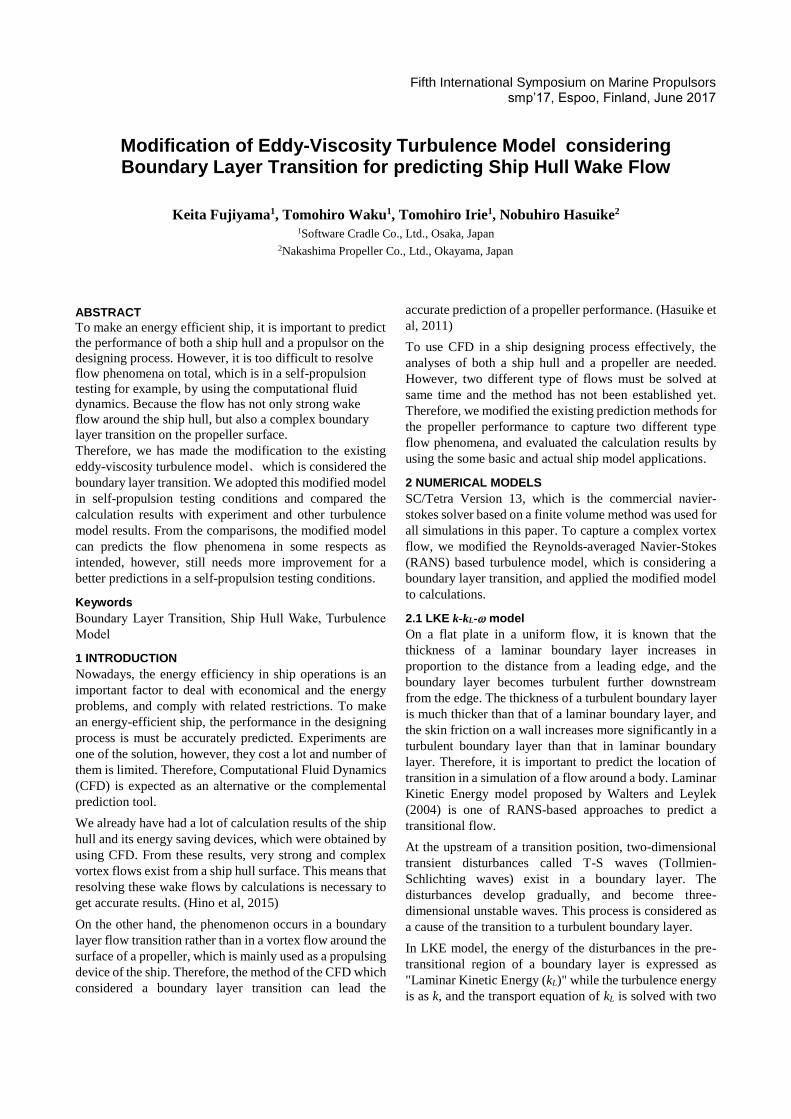
same flow regions like Figure 1 and different inlet

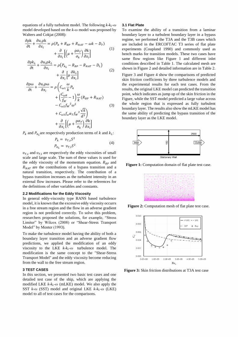
conditions described in Table 1. The calculated mesh are

shown in Figure 2 and detailed information are in Table 2.

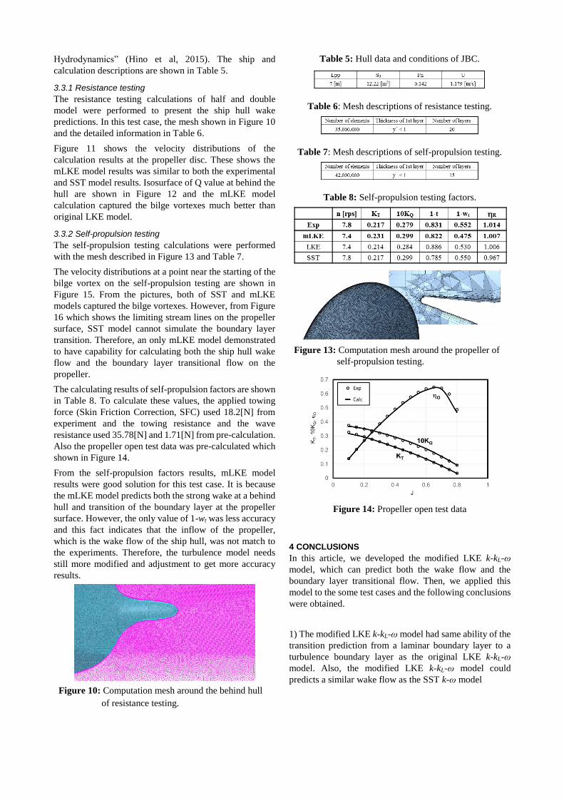
Figure 3 and Figure 4 show the comparisons of predicted

skin friction coefficients by three turbulence models and

the experimental results for each test cases. From the

results, the original LKE model can predicted the transition

point, which indicates as jump up of the skin friction in the

Figure, while the SST model predicted a large value across

the whole region that is expressed as fully turbulent

boundary layer. The results also show the mLKE model has

the same ability of predicting the bypass transition of the

boundary layer as the LKE model.

Figure 1: Computation domain of flat plate test case.

Figure 2: Computation mesh of flat plate test case.

Figure 3: Skin friction distributions at T3A test case

Figure 4: Skin friction distributions at T3B test case

Table 1: Test conditions of flat plate test cases

Table 2: Mesh descriptions of flat plate test cases

3.2 Two Dimensional Compressor Cascade

This experiments performed by Zierke and Deutsch

(1989), and the flow regions and test conditions for this

comparison are shown in Figure 5 and Table 3. In Figure 6

and Table 4, the calculated mesh and its information are

described.

Figure 7 shows the pressure distributions on the blade

surface and all of the turbulence models can predict the

surface pressure. Also, both LKE and mLKE models can

predict the boundary layer transition at mid-chord of the

blade from Figure 8, which shows the skin friction

distributions at the pressure side.

Figure 9 shows the wake flow distributions at 106% and

131.9% chord. From this results, no models can resolve the

wakes perfectly. However mLKE model had stronger wake

prediction than LKE model and the aim of the mLKE

model was realized.

Figure 5: Computation domain of compressor cascade

Figure 6: Computation mesh at blade edge.

Figure 7: Surface pressure distributions.

Figure 8: Skin friction distributions

on the pressure surface.

Figure 9: Wake distributions behind the blade

Table 3: Test condition of compressor cascade.

Table 4: Mesh descriptions of compressor.

Table 5: Hull data and conditions of JBC.

3.3 Japan Bulk Carrier (JBC) Test Case

We performed the calculation of the resistance and the self-

propulsion testing of the Japan bulk carrier (JBC), which

was used on “Tokyo 2015, A Workshop on CFD in Ship

Hydrodynamics” (Hino et al, 2015). The ship and

calculation descriptions are shown in Table 5.

3.3.1 Resistance testing

The resistance testing calculations of half and double

model were performed to present the ship hull wake

predictions. In this test case, the mesh shown in Figure 10

and the detailed information in Table 6.

Figure 11 shows the velocity distributions of the

calculation results at the propeller disc. These shows the

mLKE model results was similar to both the experimental

and SST model results. Isosurface of Q value at behind the

hull are shown in Figure 12 and the mLKE model

calculation captured the bilge vortexes much better than

original LKE model.

3.3.2 Self-propulsion testing

The self-propulsion testing calculations were performed

with the mesh described in Figure 13 and Table 7.

The velocity distributions at a point near the starting of the

bilge vortex on the self-propulsion testing are shown in

Figure 15. From the pictures, both of SST and mLKE

models captured the bilge vortexes. However, from Figure

16 which shows the limiting stream lines on the propeller

surface, SST model cannot simulate the boundary layer

transition. Therefore, an only mLKE model demonstrated

to have capability for calculating both the ship hull wake

flow and the boundary layer transitional flow on the

propeller.

The calculating results of self-propulsion factors are shown

in Table 8. To calculate these values, the applied towing

force (Skin Friction Correction, SFC) used 18.2[N] from

experiment and the towing resistance and the wave

resistance used 35.78[N] and 1.71[N] from pre-calculation.

Also the propeller open test data was pre-calculated which

shown in Figure 14.

From the self-propulsion factors results, mLKE model

results were good solution for this test case. It is because

the mLKE model predicts both the strong wake at a behind

hull and transition of the boundary layer at the propeller

surface. However, the only value of 1-wt was less accuracy

and this fact indicates that the inflow of the propeller,

which is the wake flow of the ship hull, was not match to

the experiments. Therefore, the turbulence model needs

still more modified and adjustment to get more accuracy

results.

Figure 10: Computation mesh around the behind hull

of resistance testing.

Table 5: Hull data and conditions of JBC.

Table 6: Mesh descriptions of resistance testing.

Table 7: Mesh descriptions of self-propulsion testing.

Table 8: Self-propulsion testing factors.

Figure 13: Computation mesh around the propeller of

self-propulsion testing.

Figure 14: Propeller open test data

4 CONCLUSIONS

In this article, we developed the modified LKE k-kL-ω

model, which can predict both the wake flow and the

boundary layer transitional flow. Then, we applied this

model to the some test cases and the following conclusions

were obtained.

1) The modified LKE k-kL-ω model had same ability of the

transition prediction from a laminar boundary layer to a

turbulence boundary layer as the original LKE k-kL-ω

model. Also, the modified LKE k-kL-ω model could

predicts a similar wake flow as the SST k-ω model

2) Using these characteristics, the modified LKE k-kL-ω

model well predicted to the flow both around the ship and

the propeller.

3) The prediction of some self-propulsion factors could be

significantly improved by the modified LKE k-kL-ω model

as intended, however, some interaction factors were got

worse conversely. Therefore, the adjustment and the

consideration are still needed to get more accuracy results.

REFERENCES

Coupland, J. (1990). ‘T3A and T3B Test Cases’.

ERCOFTAC Special Interest Group on Laminar to

Turbulent Transition and Retransition, A309514

Hasuike, N., Yamasaki, S. and Ando, J. (2011).

‘Numerical and Experimental Investigation into

Propulsion and Cavitation Performance of Marine

Propeller’. Proceedings of the ARINE 2011, IV

International Conferenve on Computational Methods

in Marine Engineering, pp. 199-215.

Hino, T., et al. (eds.) (2015). Tokyo 2015 A Workshop

on CFD in Ship Hydrodynamics, Tokyo, Japan.

Menter, F. (1993). ‘Zonal Two Equation k- Turbulence

Models for Aerodynamic Flows ’. AIAA Paper, 1993-

2906.

Walters, D.K. and Cokljat, D. (2008). ‘A Three-Equation

Eddy-Viscosity Model for Reynolds-Averaged

Navier-Stokes Simulations of Transitional Flow’.

ASME J. of Fluids Eng. 130, 121401.

Walters, D.K. and Leylek, J.H.(2004). ‘A New Model for

Boundary Layer Transition Using a Single-Point

RANS Approach’. ASME Journal of Turbomachinery

126, pp. 193-202.

Wilcox, D. C. (2008). ‘Formulation of the k- Turbulence

Model Revisited’. AIAA Journal 46, No. 11, pp.

2823-2838.

Zierke, W.C. & Deutsch, S. (1989). ‘The measurement of

boundary layers on a compressor blade in cascade -

Vols. 1 and 2’. NASA CR, 185118

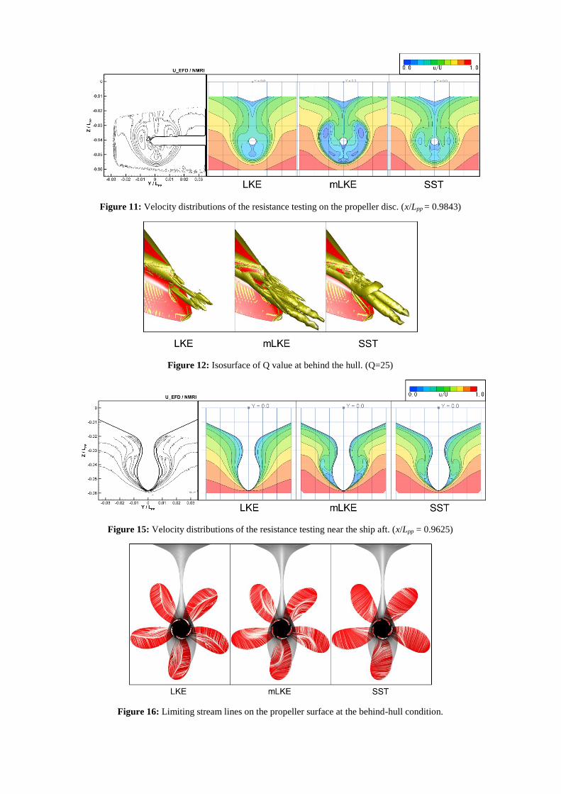
Figure 11: Velocity distributions of the resistance testing on the propeller disc. (x/Lpp = 0.9843)

Figure 12: Isosurface of Q value at behind the hull. (Q=25)

Figure 15: Velocity distributions of the resistance testing near the ship aft. (x/Lpp = 0.9625)

Figure 16: Limiting stream lines on the propeller surface at the behind-hull condition.