Modiﬁed QML Estimation of Spatial Autoregressive … Publications...While heteroskedasticity is...

Modified QML Estimation of Spatial Autoregressive Modelswith Unknown Heteroskedasticity and Nonnormality∗

Shew Fan Liu and Zhenlin Yang†

School of Economics, Singapore Management University, 90 Stamford Road, Singapore 178903.

emails: [email protected]; [email protected]

January, 2015

AbstractIn the presence of heteroskedasticity, Lin and Lee (2010) show that the quasi maximum

likelihood (QML) estimator of the spatial autoregressive (SAR) model can be inconsistentas a ‘necessary’ condition for consistency can be violated, and thus propose robust GMMestimators for the model. In this paper, we first show that this condition may hold incertain situations and when it does the regular QML estimator can still be consistent. Incases where this condition is violated, we propose a simple modified QML estimation methodrobust against unknown heteroskedasticity. In both cases, asymptotic distributions of theestimators are derived, and methods for estimating robust variances are given, leading torobust inferences for the model. Extensive Monte Carlo results show that the modified QMLestimator outperforms the GMM and QML estimators even when the latter is consistent.The proposed methods are then extended to the more general SARAR models.

Key Words: Spatial dependence; Unknown heteroskedasticity; Nonnormality, ModifiedQML estimator; Robust standard error; SARAR models.

JEL Classification: C10, C13, C15, C21

1. Introduction

Spatial dependence is increasingly becoming an integral part of empirical works in economicsas a means of modelling the effects of ‘neighbours’ (see, e.g., Cliff and Ord (1972, 1973, 1981),Ord (1975), Anselin (1988, 2003), Anselin and Bera (1998), LeSage and Pace (2009) for someearly and comprehensive works). Spatial interaction in general can occur in many forms. Forinstance peer interaction can cause stratified behaviour in the sample such as herd behaviourin stock markets, innovation spillover effects, localized purchase decisions, etc., while spatialrelationships can also occur more naturally due to structural differences in space/cross-sectionsuch as geographic proximity, trade agreements, demographic characteristics, etc. See Case(1991), Pinkse and Slade (1998), Pinkse et al. (2002), Hanushek et al. (2003), Baltagi etal. (2007) to name a few. Among the various spatial econometrics models that have beenextensively treated, the most popular one may be the spatial autoregressive (SAR) model.

∗The authors are grateful to School of Economics, Singapore Management University, for research support,and to Editor, Daniel McMillen, a referee, and the participants of the VIII world conference of the SpatialEconometrics Association, Zurich 2014, for helpful comments.

†Corresponding author: 90 Stamford Road, Singapore 178903. Phone +65-6828-0852; Fax: +65-6828-0833.

Accepted Version for Regional Science and Urban Economics

While heteroskedasticity is common in regular cross-section studies, it may be more so fora spatial econometrics model due to aggregation, clustering, etc. Anselin (1988) identifies thatheteroskedasticity can broadly occur due to “idiosyncrasies in model specification and affectthe statistical validity of the estimated model”. This may be due to the misspecification of themodel that feeds to the disturbance term or may occur more naturally in the presence of peerinteractions. Data related heteroskedasticity may also occur for example if the model deals witha mix of aggregate and non aggregate data, the aggregation may cause errors to be heteroskedas-tic. See, e.g., Glaeser et al. (1996), LeSage and Pace (2009), Lin and Lee (2010), Kelejian andPrucha (2010), for more discussions. As such, the assumption of homoskedastic disturbances islikely to be invalid in a spatial context in general. However, much of the present spatial econo-metrics literature has focused on estimators developed under the assumption that the errors arehomoskedastic. This is in a clear contrast to the standard cross-section econometrics literaturewhere the use of heteroskedasticity robust estimators is a standard practice.

Although Anselin raised the issue of heteroskedasticity in spatial models as early as in 1988,and made an attempt to provide tests of spatial effects robust to unknown heteroskedasticity,comprehensive treatments of estimation related issues were not considered until recent years by,e.g., Kelejian and Prucha (2007, 2010), LeSage (1997), Lin and Lee (2010), Arraiz et al. (2010),Badinger and Egger (2011), Jin and Lee (2012), Baltagi and Yang (2013b), and Dogan andTaspinar (2014). Lin and Lee (2010) formally illustrate that the traditional quasi maximumlikelihood (QML) and generalized method of moments (GMM) estimators are inconsistent ingeneral when the SAR model suffers from heteroskedasticity, and provide heteroskedasticityrobust GMM estimators by modifying the usual quadratic moment conditions.

Inspired by Lin and Lee (2010), we introduce a modified QML estimator (QMLE) for theSAR model by modifying the concentrated score function for the spatial parameter to make itrobust against unknown heteroskedasticity. It turns out that the method is very simple and moreimportantly, it can be easily generalized to suit more general models.1 For heteroskedasticityrobust inferences, we propose an outer-product-of-gradient (OPG) method for estimating thevariance of the modified QMLE. We provide formal theories for the consistency and asymptoticnormality of the proposed estimator, and the consistency of the robust standard error estimate.Extensive Monte Carlo results show that the modified QML estimator generally outperforms itsGMM counter parts in terms of efficiency and sensitivity to the magnitude of model parametersin particular the regression coefficients. The Monte Carlo results also show that the proposedrobust standard error estimate performs well. We also study the cases under which the regu-lar QMLE is robust against unknown heteroskedasticity and provide a set of robust inferencemethods. It is interesting to note that the modified QMLE is computationally as simple as theregular QMLE, and it also outperforms the regular QMLE when the latter is heteroskedasticityrobust. This is because the modified QMLE captures the extra variability inherent from the

1The efficiency of an MLE may be the driving force for exploiting a likelihood-based estimator for achievingrobustness against various model misspecifications such as heteroskedasticity and nonnormality. The computa-tional complexity may be the key factor that hinders the application of the ML-type estimation method. However,with the modern computing technologies this is no longer an issue of major concern, unless n is very large.

2


estimation of the regression coefficients and the average of error variances.To demonstrate their flexibility and generality, the proposed methods are then extended to

the popular spatial autoregressive model with spatial autoregressive disturbances (SARAR(1,1))with heteroskedastic innovations. Kelejian and Prucha (2010) formally treat this model with athree-step estimation procedure. Monte Carlo results show that the modified QMLE performsbetter in finite sample than the three-step estimator. Further possible extensions of the proposedmethods are discussed. In summary, the proposed set of QML-based robust inference methodsare simple and reliable, and can be easily adopted by applied researchers.

The rest of the paper is organized as follows. Section 2 examines the cases where theregular QML estimator of the SAR model is consistent under unknown heteroskedasticity, andprovides methods for robust inferences. Section 3 introduces the modified QML estimatorthat is generally robust against unknown heteroskedasticity, and presents methods for robustinferences. Section 4 presents the Monte Carlo results for the SAR model. Section 5 extends theproposed methods to the popular SARAR(1,1) model and discusses further possible extensions.Section 6 concludes the paper. All technical details are given in Appendix B.

2. QML Estimation of Spatial Autoregressive Models

In this section, we first outline the QML estimation of the SAR model under the assump-tions that the errors are independent and identically distributed (iid). Then, we examine theproperties of the QMLE of the SAR model when the errors are independent but not iden-tically distributed (inid). We provide conditions under which the regular QMLE is robustagainst heteroskedasticity of unknown form, derive its asymptotic distribution, and provideheteroskedasticity robust estimator of its asymptotic variance.

Some general notation will be followed in this paper: | · | and tr(·) denote, respectively,the determinant and trace of a square matrix; A′ denotes the transpose of a matrix A; diag(·)denotes the diagonal matrix formed by a vector or the diagonal elements of a square matrix;diagv(·) denotes the column vector formed by the diagonal elements of a square matrix; and avector raised to a certain power is operated elementwise.

2.1 The model and the QML estimation

Consider the spatial autoregressive or SAR model of the form:

Yn = λ0WnYn +Xnβ0 + εn, (1)

where Xn is an n×k matrix of exogenous variables, Wn is a known n×n spatial weights matrix,εn is an n × 1 vector of disturbances of independent and identically distributed (iid) elementswith mean zero and variance σ2, β is a k×1 vector of regression coefficients and λ is the spatialparameter. The Gaussian loglikelihood of θ = (β′, σ2, λ)′ is,

�n(θ) = −n2

ln(2π)− n

2ln(σ2) + ln |An(λ)| − 1

2σ2ε′n(β, λ)εn(β, λ), (2)

3


where An(λ) = In −λWn, In is an n×n identity matrix, and εn(β, λ) = An(λ)Yn−Xnβ. Givenλ, �n(θ) is maximized at βn(λ) = (X ′

nXn)−1X ′nAn(λ)Yn and σ2

n(λ) = 1nY

′nA

′n(λ)MnAn(λ)Yn,

where Mn = In − Xn(X ′nXn)−1X ′

n. By substituting βn(λ) and σ2n(λ) into �n(θ), we arrive at

the concentrated Gaussian loglikelihood function for λ as,

�cn(λ) = −n2

[ln(2π) + 1] − n

2ln(σ2

n(λ)) + ln |An(λ)|. (3)

Maximizing �cn(λ) gives the unconstrained QMLE λn of λ, and thus the QMLEs of β and σ2 asβn ≡ β(λn) and σ2

n ≡ σ2n(λn). Denote θn = (β′n, σ2

n, λn)′, the QMLE of θ.Under regularity conditions, Lee (2004) establishes the consistency and asymptotic normality

of the QMLE θn. In particular, he shows that λn and βn may have a slower than√n-rate of

convergence if the degree of spatial dependence (or the number of neighbours each spatial unithas) grows with the sample size n. The QMLE and its asymptotic distribution developedby Lee are robust against nonnormality of the error distribution. However, some importantissues need to be further considered: (i) conditions under which the regular QMLE θn remainsconsistent when errors are heteroskedastic, (ii) methods to modify the regular QMLE θn sothat it becomes generally consistent under unknown heteroskedasticity, and (iii) methods forestimating the variance of the (modified) QMLE robust against unknown heteroskedasticity.

2.2 Robustness of QMLE against unknown heteroskedasticity

It is accepted that the regular QMLE of the usual linear regression model without spatialdependence, developed under homoskedastic errors, is still consistent when the errors are in factheteroskedastic. However, for correct inferences the standard error of the estimator has to beadjusted to account for this unknown heteroskedasticity (White, 1980). Suppose now we havea linear regression model with spatial dependence as given in (1) with disturbances that areinid with means zero and variances σ2hn,i, i = 1, . . . , n, where hn,i > 0 and 1

n

∑ni=1 hn,i = 1.2

Consider the score function derived from (2),

ψn(θ) =∂�n(θ)∂θ

=

⎧⎪⎪⎪⎨⎪⎪⎪⎩

1σ2X

′nεn(β, λ),

12σ4 [ε′n(β, λ)εn(β, λ)− nσ2],1σ2Y

′nW

′nεn(β, λ)− tr[Gn(λ)],

(4)

where Gn(λ) = WnA−1(λ). It is well known that for an extremum estimator, such as the

QMLE θn we consider, to be consistent, a necessary condition is that plimn→∞1nψn(θ0) = 0 at

the true parameter θ0 (Amemiya, 1985). This is always the case for the β and σ2 componentsof ψn(θ0) whether or not the errors are homoskedastic. However, it may not be the case forthe λ component of ψn(θ0). Let hn = (hn,1, . . . , hn,n)′, gn = (gn,1, . . . , gn,n)′ = diagv(Gn),gn = 1

n

∑ni=1 gn,i, Hn = diag(hn). Let Cov(gn, hn) denote the sample covariance between the

2Note that σ2 is the average of Var(εn,i). Under homoskedasticity, hn,i = 1,∀i. For generality, we allow hn,i

to depend on n, for each i. This parameterization, a nonparametric version of Breusch and Pagan (1979), isuseful as it allows the estimation of the average scale parameter. See Section 3 for more details.

4


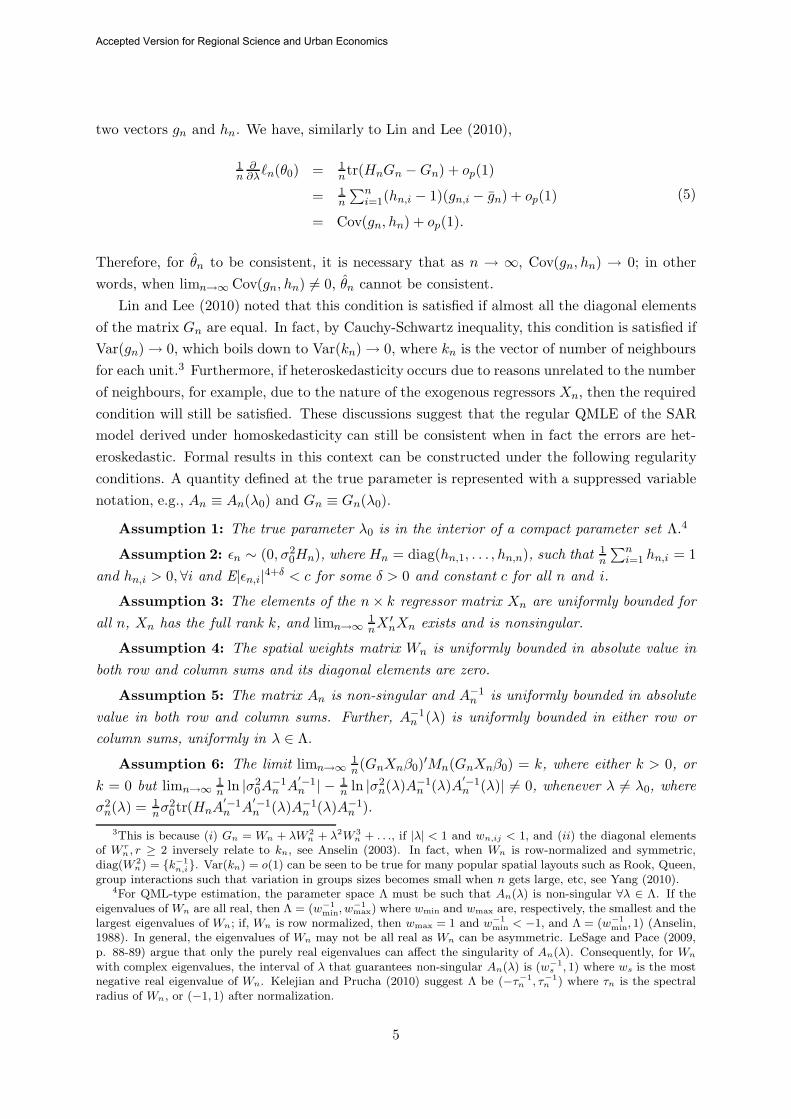
two vectors gn and hn. We have, similarly to Lin and Lee (2010),

1n

∂∂λ�n(θ0) = 1

ntr(HnGn −Gn) + op(1)

= 1n

∑ni=1(hn,i − 1)(gn,i − gn) + op(1)

= Cov(gn, hn) + op(1).

(5)

Therefore, for θn to be consistent, it is necessary that as n → ∞, Cov(gn, hn) → 0; in otherwords, when limn→∞ Cov(gn, hn) �= 0, θn cannot be consistent.

Lin and Lee (2010) noted that this condition is satisfied if almost all the diagonal elementsof the matrix Gn are equal. In fact, by Cauchy-Schwartz inequality, this condition is satisfied ifVar(gn) → 0, which boils down to Var(kn) → 0, where kn is the vector of number of neighboursfor each unit.3 Furthermore, if heteroskedasticity occurs due to reasons unrelated to the numberof neighbours, for example, due to the nature of the exogenous regressors Xn, then the requiredcondition will still be satisfied. These discussions suggest that the regular QMLE of the SARmodel derived under homoskedasticity can still be consistent when in fact the errors are het-eroskedastic. Formal results in this context can be constructed under the following regularityconditions. A quantity defined at the true parameter is represented with a suppressed variablenotation, e.g., An ≡ An(λ0) and Gn ≡ Gn(λ0).

Assumption 1: The true parameter λ0 is in the interior of a compact parameter set Λ.4

Assumption 2: εn ∼ (0, σ20Hn), where Hn = diag(hn,1, . . . , hn,n), such that 1

n

∑ni=1 hn,i = 1

and hn,i > 0, ∀i and E|εn,i|4+δ < c for some δ > 0 and constant c for all n and i.

Assumption 3: The elements of the n× k regressor matrix Xn are uniformly bounded forall n, Xn has the full rank k, and limn→∞ 1

nX′nXn exists and is nonsingular.

Assumption 4: The spatial weights matrix Wn is uniformly bounded in absolute value inboth row and column sums and its diagonal elements are zero.

Assumption 5: The matrix An is non-singular and A−1n is uniformly bounded in absolute

value in both row and column sums. Further, A−1n (λ) is uniformly bounded in either row or

column sums, uniformly in λ ∈ Λ.

Assumption 6: The limit limn→∞ 1n(GnXnβ0)′Mn(GnXnβ0) = k, where either k > 0, or

k = 0 but limn→∞ 1n ln |σ2

0A−1n A

′−1n | − 1

n ln |σ2n(λ)A−1

n (λ)A′−1n (λ)| �= 0, whenever λ �= λ0, where

σ2n(λ) = 1

nσ20tr(HnA

′−1n A

′−1n (λ)A−1

n (λ)A−1n ).

3This is because (i) Gn = Wn + λW 2n + λ2W 3

n + . . ., if |λ| < 1 and wn,ij < 1, and (ii) the diagonal elementsof W r

n , r ≥ 2 inversely relate to kn, see Anselin (2003). In fact, when Wn is row-normalized and symmetric,diag(W 2

n) = {k−1n,i}. Var(kn) = o(1) can be seen to be true for many popular spatial layouts such as Rook, Queen,

group interactions such that variation in groups sizes becomes small when n gets large, etc, see Yang (2010).4For QML-type estimation, the parameter space Λ must be such that An(λ) is non-singular ∀λ ∈ Λ. If the

eigenvalues of Wn are all real, then Λ = (w−1min, w

−1max) where wmin and wmax are, respectively, the smallest and the

largest eigenvalues of Wn; if, Wn is row normalized, then wmax = 1 and w−1min < −1, and Λ = (w−1

min, 1) (Anselin,1988). In general, the eigenvalues of Wn may not be all real as Wn can be asymmetric. LeSage and Pace (2009,p. 88-89) argue that only the purely real eigenvalues can affect the singularity of An(λ). Consequently, for Wn

with complex eigenvalues, the interval of λ that guarantees non-singular An(λ) is (w−1s , 1) where ws is the most

negative real eigenvalue of Wn. Kelejian and Prucha (2010) suggest Λ be (−τ−1n , τ−1

n ) where τn is the spectralradius of Wn, or (−1, 1) after normalization.

5


Assumptions 2 and 3 are similar to those from Lin and Lee (2010). Assumption 2 im-plies that {hn,i} as well as the third and fourth moments of εn,i are uniformly bounded forall n and i. Assumptions 2 and 3 imply that limn→∞ 1

nX′nHnXn exists and is nonsingular.

Assumptions 4 and 5 are standard for the SAR model. The uniform boundedness conditionslimit the spatial dependence to a manageable level (Kelejian and Prucha, 1999). Assumption6 is the heteroskedastic version of the identification condition introduced by Lee (2004) for thehomoskedastic SAR model.

For the loglikelihood and score functions given in (2) and (4), let In = − 1nE

[∂2

∂θ∂θ′ �n(θ0)]

and Σn = 1nE

[∂∂θ�n(θ0) ∂

∂θ′ �n(θ0)], with their exact expressions deferred to the next subsection

in connection with the issue on the robust variance covariance matrix estimation. We have thefollowing results (recall gn = diagv(Gn) and let qn = diagv(G′

nGn)).

Theorem 1: Under Assumptions 1-6, Cov(gn, hn) = o(1) and Cov(qn, hn) = o(1), we haveas n→ ∞, θn

p−→ θ0; under Assumptions 1-6 and Cov(gn, hn) = o(n−1/2), we have as n→ ∞,

√n(θn − θ0)

D−→ N (0, I−1Σ I−1), (6)

where I = limn→∞ In and Σ = limn→∞ Σn both assumed to exist and I is nonsingular.

2.3 Robust standard errors of the QML estimators

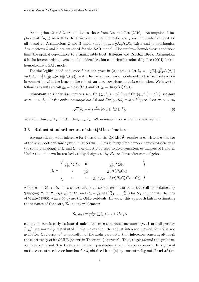
Asymptotically valid inference for θ based on the QMLEs θn requires a consistent estimatorof the asymptotic variance given in Theorem 1. This is fairly simple under homoskedasticity asthe sample analogue of In and Σn can directly be used to give consistent estimators of I and Σ.Under the unknown heteroskedasticity designated by Hn, we have after some algebra:

In =

⎛⎜⎜⎜⎝

1σ20nX ′

nXn 0 1σ20nX ′

nηn

∼ 12σ4

0

1σ20n

tr(HnGn)

∼ ∼ 1σ20nη′nηn + 1

n tr(HnG′nGn +G2

n)

⎞⎟⎟⎟⎠ ,

where ηn = GnXnβ0. This shows that a consistent estimator of In can still be obtained by‘plugging’ θn for θ0, Gn(θn) for Gn and Hn = 1

σ2ndiag(ε2n,1, . . . , ε

2n,n) for Hn, in line with the idea

of White (1980), where {εn,i} are the QML residuals. However, this approach fails in estimatingthe variance of the score, Σn, as its σ2

0-element:

Σn,σ2σ2 = 14nσ4

0

∑ni=1(κn,i + 2h2

n,i),

cannot be consistently estimated unless the excess kurtosis measures {κn,i} are all zero or{εn,i} are normally distributed. This means that the robust inference method for σ2

0 is notavailable. Obviously, σ2 is typically not the main parameter that inferences concern, althoughthe consistency of its QMLE (shown in Theorem 1) is crucial. Thus, to get around this problem,we focus on λ and β as those are the main parameters that inferences concern. First, basedon the concentrated score function for λ, obtained from (4) by concentrating out β and σ2 (see

6


(7) below), we obtain the robust variance of λn, and then based on the relationship between βn

and λn we obtain the robust variance of βn. As these developments fall into the main resultspresented in next section, we give details at the end of Section 3.3.

3. Modified QML Estimation under Heteroskedasticity

As argued in Lin and Lee (2010) and further discussed in Section 2 of this paper, the nec-essary condition for the consistency of the regular QMLE, limn→∞ Cov(gn, hn) = 0, can beviolated when hn is proportional to the number of neighbours kn for each spatial unit andlimn→∞ Var(kn) �= 0.5 To solve this problem, Lin and Lee (2010) propose robust GMM andoptimal robust GMM estimators for the SAR model. In this paper, we introduce a modifiedQMLE for the SAR model by modifying the concentrated score function for the spatial param-eter to make it robust against unknown heteroskedasticity. It turns out that the method isvery simple and more importantly it can be easily generalized to suit more general models (seeSection 5). Furthermore, the method of modification takes into account the estimation of theβ and σ2 parameters, thus can be expected to have a good finite sample performance. Indeed,the Monte Carlo results presented in Section 4 show an excellent finite sample performance ofthe proposed estimator. For robust inferences concerning the spatial or regression parameters,we introduce OPG estimators of the variances of the modified QMLEs.

3.1 The modified QML Estimator

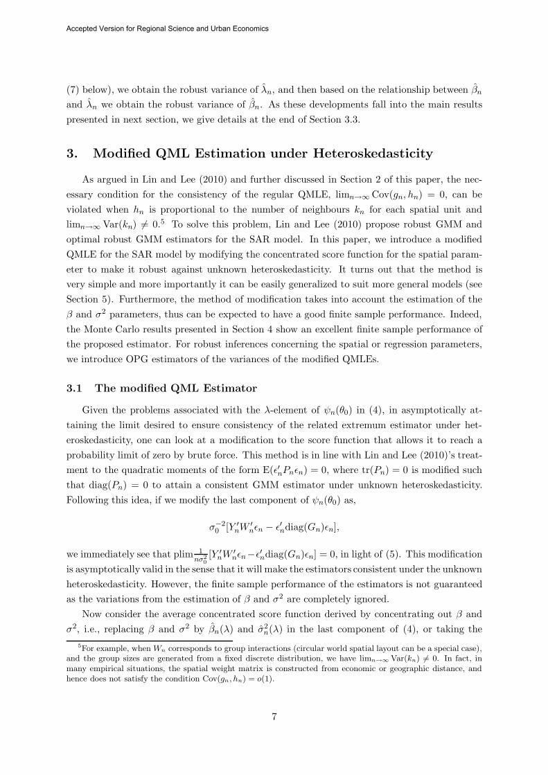
Given the problems associated with the λ-element of ψn(θ0) in (4), in asymptotically at-taining the limit desired to ensure consistency of the related extremum estimator under het-eroskedasticity, one can look at a modification to the score function that allows it to reach aprobability limit of zero by brute force. This method is in line with Lin and Lee (2010)’s treat-ment to the quadratic moments of the form E(ε′nPnεn) = 0, where tr(Pn) = 0 is modified suchthat diag(Pn) = 0 to attain a consistent GMM estimator under unknown heteroskedasticity.Following this idea, if we modify the last component of ψn(θ0) as,

σ−20 [Y ′

nW′nεn − ε′ndiag(Gn)εn],

we immediately see that plim 1nσ2

0[Y ′

nW′nεn−ε′ndiag(Gn)εn] = 0, in light of (5). This modification

is asymptotically valid in the sense that it will make the estimators consistent under the unknownheteroskedasticity. However, the finite sample performance of the estimators is not guaranteedas the variations from the estimation of β and σ2 are completely ignored.

Now consider the average concentrated score function derived by concentrating out β andσ2, i.e., replacing β and σ2 by βn(λ) and σ2

n(λ) in the last component of (4), or taking the5For example, when Wn corresponds to group interactions (circular world spatial layout can be a special case),

and the group sizes are generated from a fixed discrete distribution, we have limn→∞ Var(kn) �= 0. In fact, inmany empirical situations, the spatial weight matrix is constructed from economic or geographic distance, andhence does not satisfy the condition Cov(gn, hn) = o(1).

7


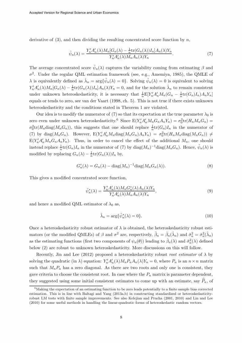
derivative of (3), and then dividing the resulting concentrated score function by n,

ψn(λ) =Y ′

nA′n(λ)Mn[Gn(λ)− 1

n tr(Gn(λ))In]An(λ)Yn

Y ′nA

′n(λ)MnAn(λ)Yn

. (7)

The average concentrated score ψn(λ) captures the variability coming from estimating β andσ2. Under the regular QML estimation framework (see, e.g., Amemiya, 1985), the QMLE ofλ is equivalently defined as λn = arg{ψn(λ) = 0}. Solving ψn(λ) = 0 is equivalent to solvingY ′

nA′n(λ)Mn[Gn(λ) − 1

ntr(Gn(λ))In]An(λ)Yn = 0, and for the solution λn to remain consistentunder unknown heteroskedasticity, it is necessary that 1

nE[Y ′nA

′nMn(Gn − 1

ntr(Gn)In)AnYn]equals or tends to zero, see van der Vaart (1998, ch. 5). This is not true if there exists unknownheteroskedasticity and the conditions stated in Theorem 1 are violated.

Our idea is to modify the numerator of (7) so that its expectation at the true parameter λ0 iszero even under unknown heteroskedasticity.6 Since E(Y ′

nA′nMnGnAnYn) = σ2

0tr(HnMnGn) =σ2

0tr(Hndiag(MnGn)), this suggests that one should replace 1ntr(Gn)In in the numerator of

(7) by diag(MnGn). However, E(Y ′nA

′nMndiag(MnGn)AnYn) = σ2

0tr(HnMndiag(MnGn)) �=E(Y ′

nA′nMnGnAnYn). Thus, in order to cancel the effect of the additional Mn, one should

instead replace 1n tr(Gn)In in the numerator of (7) by diag(Mn)−1diag(MnGn). Hence, ψn(λ) is

modified by replacing Gn(λ)− 1ntr(Gn(λ))In by,

G◦n(λ) = Gn(λ)− diag(Mn)−1diag(MnGn(λ)). (8)

This gives a modified concentrated score function,

ψ∗n(λ) =

Y ′nA

′n(λ)MnG

◦n(λ)An(λ)Yn

Y ′nA

′n(λ)MnAn(λ)Yn

, (9)

and hence a modified QML estimator of λ0 as,

λn = arg{ψ∗n(λ) = 0}. (10)

Once a heteroskedasticity robust estimator of λ is obtained, the heteroskedasticity robust esti-mators (or the modified QMLEs) of β and σ2 are, respectively, βn = βn(λn) and σ2

n = σ2n(λn)

as the estimating functions (first two components of ψn(θ)) leading to βn(λ) and σ2n(λ) defined

below (2) are robust to unknown heteroskedasticity. More discussions on this will follow.Recently, Jin and Lee (2012) proposed a heteroskedasticity robust root estimator of λ by

solving the quadratic (in λ) equation: Y ′nA

′n(λ)MnPnAn(λ)Yn = 0, where Pn is an n×n matrix

such that MnPn has a zero diagonal. As there are two roots and only one is consistent, theygave criteria to choose the consistent root. In case where the Pn matrix is parameter dependent,they suggested using some initial consistent estimates to come up with an estimate, say Pn, of

6Making the expectation of an estimating function to be zero leads potentially to a finite sample bias correctedestimation. This is in line with Baltagi and Yang (2013a,b) in constructing standardized or heteroskedasticity-robust LM tests with finite sample improvements. See also Kelejian and Prucha (2001, 2010) and Lin and Lee(2010) for some useful methods in handling the linear-quadratic forms of heteroskedastic random vectors.

8


Pn, and then solve Y ′nA

′n(λ)MnPnAn(λ)Yn = 0. Clearly, G◦

n(λ) defined above is a choice forPn although an initial estimate of λ, say λ0

n, is needed to obtain Pn = G◦n(λ0

n). Jin and Leealso suggest this. This approach is attractive as the root estimator has a closed-form expressionand thus can handle a super large data. However, it can be ambiguous in practice in choosinga consistent root as the selection criterion is parameter dependent. Furthermore, our MonteCarlo simulation shows that Y ′

nA′n(λ)MnPnAn(λ)Yn = 0 tends to give non-real roots when |λ|

is not small, say ≥ 0.5, in particular when λ is negative, and when n is not very large. Incontrast, this problem does not occur to the modified QML estimator λn given above. Thus,the modified QML estimator λn proposed in this paper complements Jin and Lee’s (2012) rootestimator. More discussions along this line are given in the following sections. Some remarksfollow before moving into the asymptotic properties of the modified QML estimators.

Remark 1: It turns out that the modified QMLEs of the SAR model are computation-ally as simple as the original QMLEs, but the former are generally consistent under unknownheteroskedasticity while preserving the nature of being robust against nonnormality.

Remark 2: The proposed methods can be easily extended to more advanced models (spatialor non-spatial) as demonstrated in Section 5. However, it is not clear to us how to extend theGMM estimators of Lin and Lee (2010) to a more general model, and the root estimator of Jinand Lee (2012) may run into difficulty for a more general model as when there are two (or more)quadratic functions of two (or more) unknowns, it is difficult to choose the consistent roots.

Remark 3: The correction G◦n(λ) = Gn(λ)−diag(Mn)−1diag(MnGn(λ)) as opposed to the

more intuitively appealing correction Gn(λ)−diag(Gn(λ)) has better finite sample performancesince the modification is made directly on the concentrated score function which contains thevariability accruing from the estimation of β and σ2.

3.2 Asymptotic distribution of the modified QML estimators

To ensure that the modified estimation function given in (9) uniquely identifies λ0, theAssumption 6 needs to be modified as follows. Let Ωn(λ) = A′

n(λ)[Gn(λ)− diag(Gn(λ))]An(λ).

Assumption 6∗: limn→∞

1n [β′0X

′nA

′−1n Ωn(λ)A−1

n Xnβ0+σ20tr(HnA

′−1n Ωn(λ)A−1

n )] �= 0, ∀λ �= λ0.

The central limit theorem (CLT) for linear quadratic forms of Kelejian and Prucha (2001)allows for heteroskedasticity and can be used to prove the asymptotic normality of the modifiedQML estimator. First, it is easy to show that the normalized and modified concentrated scorefunction has the following representation at λ0,

√nψ∗

n ≡ √nψ∗

n(λ0) = 1√nσ2

0

(ε′nBnεn + c′nεn

)+ op(1), (11)

where Bn = MnG◦n and cn = MnG

◦nXnβ0, because σ2

n(λ0) = 1nε

′nMnεn = 1

nE(ε′nMnεn)+op(1) =σ20n tr(HnMn) + op(1) = σ2

0 + op(1), and it follows that σ−2n (λ0) = σ−2

0 + op(1).Let τn(·) denote the first-order standard deviation and τ2

n(·) the first-order variance of anormalized quantity, e.g., τ2

n(ψ∗n) is the first-order term of Var(

√nψ∗

n), and τ2n(λn) is the first-

9


order term of Var(√nλn). By the representation (11) and Lemma A.3, we have,

τ2n(ψ∗

n) = 1n

∑ni=1(b

2n,iih

2n,iκn,i + 2

σ40bn,iicn,isn,i)+ 1

ntr[HnBn(HnBn +HnB′n)]+ 1

nσ20c′nHncn, (12)

where bn,ii are the diagonal elements of Bn, sn,i = E(ε3n,i), and κn,i is the excess kurtosis of εn,i

which together with Hn are defined in Section 2.3. Now by the CLT for linear-quadratic formsof Kelejian and Prucha (2001), we have,

√nψ∗

n

τn(ψ∗n)

D−→ N (0, 1). (13)

This result quickly leads to the following theorem regarding the asymptotic properties of themodified QMLE λn of the spatial parameter λ.

Theorem 2: Under Assumptions 1-5 and 6∗, the modified QML estimator λn is consistentand asymptotically normal, i.e., as n→ ∞, λn

p−→ λ0, and

√n(λn − λ0)

D−→ N(0, limn→∞ τ2

n(λn)),

where τ2n(λn) = Φ−2

n τ2n(ψ∗

n), Φn = 1ntr[Hn(G◦

nGn +G◦′nGn − G◦

n)] + 1nσ2

0c′nηn, and G◦

n = ddλG

◦n =

G2n − diag(Mn)−1diag(MnG

2n).

Now consider the modified QMLEs βn and σ2n of β0 and σ2

0 defined below (10). Using therelation An(λn) = An − (λn − λ0)Wn, we can write,

βn = βn(λ0) − (λn − λ0)(X ′nXn)−1X ′

nGnAnYn, and (14)

σ2n = σ2

n(λ0)− 2(λn − λ0) 1nY

′nW

′nMnAnYn + (λn − λ0)2 1

nY′nW

′nMnWnYn. (15)

The asymptotic properties of βn and σ2n are summarized in the following theorem. Recall

ηn = GnXnβ0 defined in Section 2.3.

Theorem 3: Under Assumptions 1-5 and 6∗, the modified QMLEs βn and σ2n are consistent,

i.e., as n→ ∞, βnp−→ β0 and σ2

np−→ σ2

0 , and further βn is asymptotically normal, i.e.,

√n(βn − β0)

D−→ N[0, limn→∞(X ′

nXn)−1X ′nAnXn(X ′

nXn)−1],

where An = nσ20Hn + τ2

n(λn)ηnη′n − 2Φ−1

n (σ−20 diag(Bn)sn +Hncn)η′n, and sn = E(ε3n).7

Clearly, the applicability of the results of Theorems 2 and 3 for making inferences for λ orβ depends on the availability of a consistent estimator of τ2

n(ψ∗n). The plug-in method based on

(12) does not work due to the involvement of higher-order moments sn,i and κn,i.

7Similarly,√

n(σ2n − σ2

0)D−→ N

`0, limn→∞ τ2

n(σ2n)

´, where the first-order variance of

√nσ2

n, τ2n(σ2

n) =1n

Pni=1 Var(ε2n,i)+

4n2 σ4

0τ2n(λn)tr2(HnGn)+ 4

n2 Cov(ε′nε, ε′nBnεn +c′nεn)tr(HnGn)Φ−1n = O(1), suggesting that σ2

n

is root-n consistent. However, similar to the regular QMLE, this result cannot be used for inference for σ20 as the

key element in the variance formula 1n

Pni=1 Var(ε2n,i) =

σ40

n

Pni=1(κn,i + 2h2

n,i) cannot be consistently estimated.

10


3.3 Robust standard errors of the modified QML estimators

Following the discussions in Section 2.3 and Footnote 7, we focus on λ and β for robustinferences. In order to carry out inference for model parameters using the modified QMLprocedure, we need a consistent estimate of τ2

n(λn). Given this, consistent estimates of τ2n(βn) =

(X ′nXn)−1X ′

nAnXn(X ′nXn)−1 immediately follow. The first-order variance of the modified score

as given in (12) contains second, third and fourth moments of εi which vary across i, and hencea simple White-type estimator (White, 1980) may not be suitable, which in turn makes τ2

n(λn)infeasible. To overcome this difficulty, we follow the idea of Baltagi and Yang (2013b) todecompose the numerator of the modified score into a sum of uncorrelated terms, and then usethe outer product of gradients (OPG) method to estimate the variance of this score functionwhich in turn leads to a consistent estimate of τ2(λn). Denote the numerator of (11) by,

Qn(εn) = ε′nBnεn + c′nεn. (16)

Clearly, Qn is not a sum of uncorrelated components, but can be made to be so by the techniqueof Baltagi and Yang (2013b). Decompose the non-stochastic matrix Bn as,

Bn = Bun + Bl

n +Bdn, (17)

where Bun , Bl

n and Bdn are, respectively, the upper triangular, the lower triangular and the

diagonal matrices of Bn. Let ζn = (Bu′n +Bl

n)εn. Then, Qn(εn) can be written as,

Qn(εn) =∑n

i=1 εn,i(ζn,i + bn,iiεn,i + cn,i), (18)

where εn,i, ζn,i and cn,i are, respectively, the elements of εn, ζn and cn. Equation (18) expressesQn(εn) as a sum of n uncorrelated terms {εn,i(ζn,i + bn,iiεn,i + cn,i)}, and hence its OPG givesa consistent estimate of the variance of Qn(εn), which in turn leads to a consistent estimate ofτ2n(ψ∗

n), the first-order variance of√nψ∗

n, as:

τ2n(ψ∗

n) = 1nσ4

n

∑ni=1

(εn,i(ζn,i + bn,iiεn,i + cn,i)

)2, (19)

where εn,i are the residuals computed from the modified QMLEs θn = (β′n, σ2n, λn)′.

Let Hn = 1σ2

ndiag(ε21n, . . . , ε

2nn). Let Φn be Φn evaluated at θn and Hn, ηn = GnXnβn, and

Gn = Gn(λn). Define the estimators of τ2n(λn) and τ2

n(βn) as,

τ2n(λn) = Φ−2

n τ2n(ψ∗

n), and (20)

τ2n(βn) = (X ′

nXn)−1X ′nAnXn(X ′

nXn)−1, (21)

where An = nσ2nHn + τ2


n (σ−2n Bd

nsn + Hncn)η′n and sn = ε3n. Note that Φn cansimply be estimated by − d

dλ0ψ∗

n|λ0=λnas Φn is the 1st-order term of −E( d

dλ0ψ∗

n).

Theorem 4: If Assumptions 1-5 and 6∗ hold, then we have as n→ ∞, τ2n(λn)−τ2

n(λn)p−→

0; and τ2n(βn) − τ2

n(βn)p−→ 0.

11


Finally, when the conditions of Theorem 1 are satisfied so the regular QMLEs are alsoconsistent, the robust variances of λn and βn can easily be obtained from the results of Theorems2-4. Some details are as follows. Starting with the concentrated score ψn given in (7), oneobtains τ2(λn) by simply replacing G◦

n by Gn − 1ntr(Gn)In in (11) and (12), and in Φn defined

in Theorem 2. Similarly, replacing G◦n by Gn − 1

n tr(Gn)In in τ2n(βn) given in Theorem 3 leads

to τ2n(βn). The estimates of τ2(λn) and τ2

n(βn) are obtained in the same way as those of τ2(λn)and τ2

n(βn), and their consistency can be proved similarly to the results of Theorem 4.

4. Monte Carlo Study

Extensive Monte Carlo experiments were conducted to (i) investigate the finite samplebehaviour of the original QMLE λn and the modified QMLE (MQMLE) λn proposed in thispaper, and their impacts on the estimators of β and σ2, with respect to the changes in thesample size, spatial layouts, error distributions and the model parameters when the models areheteroskedastic; and (ii) compare the QMLE and the MQMLE with the non-robust generalizedmethod of moments estimator (GMME) of Lee (2001), the robust GMME (RGMME) and theoptimal RGMME (ORGMME) of Lin and Lee (2010), two stage least squares estimator (2SLSE)of Kelejian and Prucha (1998), and the root estimator (RE) of Jin and Lee (2012). We considercases where the original QMLE are robust against heteroskedasticity and the cases it is not.

The simulations are carried out based on the following data generation process (DGP):

Yn = λWnYn + ιnβ0 +X1nβ1 +X2nβ2 + εn,

where ιn is an n×1 vector of ones corresponding to the intercept term, X1n and X2n are the n×1vectors containing the values of two fixed regressors, and εn = σHnen. The regression coefficientsβ is set to either (3, 1, 1)′ or (.3, .1, .1)′, σ is set to 1, λ takes values form {−0.5,−0.25, 0, 0.25, 0.5}and n take values from {100, 250, 500, 1000}. The ways of generating the values for (X1n, X2n),the spatial weights matrix Wn, the heteroskedasticity measure Hn, and the idiosyncratic errorsen are described below. Each set of Monte Carlo results is based on 1, 000 Monte Carlo samples.

Spatial Weight Matrix: We use three different spatial layouts: (i) Circular Neighbours,(ii) Group Interaction and (iii) Queen Contiguity. In (i), neighbours occur in the positionsimmediately ahead and behind a particular spatial unit. For example, for the ith spatial unitwith 6 neighbours, the ith row of Wn matrix has non-zero elements in the positions: i− 3, i−2, i− 1, i+ 1, i+ 2, and i+ 3. The weights matrix we consider has 2, 4, 6, 8 and 10 neighbourswith equal proportion. In (ii), neighbours occur in groups where each group member is spatiallyrelated to one another resulting in a symmetric Wn matrix. In (iii), neighbours could occurin the eight cardinal and ordinal positions of each unit. To ensure the heteroskedasticity effectdoes not fade as n increases (so that the regular QMLE is inconsistent), the degree of spatialdependence is fixed with respect to n. This is attained by fixing the possible group sizes inthe Group Interaction scheme, and fixing the number of neighbours behind and ahead in theCircular Neighbours scheme. The degree of spatial dependence is naturally bounded in the

12


Queen Contiguity weight matrix. To analyse the performance of the original QMLE when it isrobust against heteroskedasticity, we use Queen Contiguity scheme and the balanced Circular

Neighbours scheme where all spatial units have 6 peers each.

Heteroskedasticity: For the unbalanced Circular Neighbour scheme, hn,i is generatedas the ratio of the total number of neighbours to the average number of neighbours for each i

while for the Group Interaction scheme hn,i is generated as the ratio of the group size to meangroup size. For the balanced Circular Neighbour and the Queen Contiguity schemes, we usehn,i = n[

∑ni=1(|X1n,i| + |X2n,i|)]−1(|X1n,i| + |X2n,i|).

Regressors: The regressors are generated according to REG1: {x1i, x2i} iid∼ N (0, 1)/√

2.For the Group Interaction scheme, the regressors can also be generated according to REG2:

{x1,ir, x2,ir} iid∼ (2zr + zir)/√

10, where (zr, zir)iid∼ N (0, 1), for the ith observation in the rth

group, to give a case of non-iid regressors taking into account the impact of group sizes on theregressors. Both schemes give a signal-to-noise ratio of 1 when β1 = β2 = σ = 1.

Error Distribution: To generate the en component of the disturbance term, three DGPsare considered: DGP1: {en,i} are iid standard normal, DGP2: {en,i} are iid standardized normalmixture with 10% of values from N (0, 4) and the remaining from N (0, 1) and DGP3: {en,i} iidstandardized log-normal with parameters 0 and 1. Thus, the error distribution from DGP2 isleptokurtic, and that of DGP3 is both skewed and leptokurtic.

The GMM-type estimators are implemented by closely following Lin & Lee (2010). A GMMestimator is in general defined as a solution to the minimisation problem: minθ∈Θ g

′n(θ)a′nangn(θ)

where gn(θ) =(Qn, P1nεn(θ), . . . , Pmnεn(θ)

)′εn(θ) represents the linear and quadratic moment

conditions, Qn = (Xn, WnXn) is the matrix of instrumental variables (IVs), and a′nan is theweighting matrix related to the distance function of the minimisation problem. The GMME(Kelejian & Prucha, 1999; Lee, 2001) under homoskedastic disturbances can be defined using theusual moment condition, Pn =

(Gn − tr(Gn)

n In)

and the IVs, (GnXnβ,Xn). For the RGMME,the Pn matrix in the moment conditions changes to Gn − diag(Gn). A first step GMME withPn = Wn is used to evaluate Gn. The weighting matrices of the distance functions are computedusing the variance formula of the iid case using residual estimates given by the first step GMMestimate. The ORGMME is a variant of the RGMME in which the weighting matrix is robust tounknown heteroskedasticity. The ORGMME results given in the tables are computed using theRGMME as the initial estimate to compute the standard error estimates and the instruments.Finally, the 2SLSE uses the same IV matrix Qn. Lin and Lee (2010) gives a detailed comparisonof the finite sample performance of MLE, GMME, RGMME, ORGMME and 2SLSE for modelswith both homoskedastic and heteroskedastic errors. Our Monte Carlo experiments expandtheirs by giving a detailed investigation on the effects of nonnormality, spatial layouts as wellas negative values for the spatial parameter. The RE of Jin and Lee (2012) is also included.

To conserve space, only the partial results of QMLE, MQMLE, RGMME and ORGMMEare reported. The full set of results are available from the authors upon request. The GMMEand 2SLSE can perform very poorly. The root estimator performs equally well as the MQMLE

13


when |λ| is not large and n is not small but tends to give non-real roots otherwise. Tables 1-3summarise the estimation results for λ and Tables 4-6 for β, where in each table, the MonteCarlo means, root mean square errors (rmse) and the standard errors (se) of the estimators arereported. To analyse the finite sample performance of the proposed OPG based robust standarderror estimators, we also report the averaged se of the regular QMLE when it is heteroskedas-ticity robust and the averaged se of the MQMLE based on Theorem 4. The experiments withβ = (0.3, 0.1, 0.1) represent cases where the stochastic component is relatively more dominantthan the deterministic component of the model. This allows a comparison between the QML-type estimators and the GMM-type estimators when the model suffers from relatively moresevere heteroskedasticity and the IVs are weaker. The main observations made from the MonteCarlo results are summarized as follows:

(i) MQMLE of λ performs well in all cases considered, and it generally outperforms all otherestimators in terms of bias and rmse.8 Further, in cases where QMLE is consistent,MQMLE can be significantly less biased than QMLE, and is as efficient as QMLE.

(ii) RGMME and ORGMME of λ perform reasonably well when β = (3, 1, 1)′, but deterioratessignificantly when β = (.3, .1, .1)′ and in this case GMME and 2SLSE can be very erratic.In contrast, MQMLE is much less affected by the magnitude of β, and is less biased andmore efficient than RGMME and ORGMME more significantly when β = (.3, .1, .1)′.

(iii) RE of λ performs equally well as MQMLE when |λ| is not big and n is not small, butotherwise tends to give imaginary roots. Thus, when one encounters a super large datasetand the QMLE or MQMLE run into computational difficulty, one may turn to RE anduse its closed-form expression.

(iv) The GMM-type estimators can perform quite differently when the errors are normal asopposed to non-normal errors, especially when β = (.3, .1, .1)′. It is interesting to notethat RGMME often outperforms the ORGMME.

(v) The OPG-based estimate of the robust standard errors of MQMLE of λ performs well ingeneral with their values very close to their Monte Carlo counter parts.

(vi) Finally, the relative performance of various estimators of β is much less contrasting thanthat of various estimators of λ, although it can be seen that MQMLE of β is slightly moreefficient than the competing RGMME and ORGMME.

5. Extension to More General Models

As discussed in the introduction and Remark 2 of Section 3.1, the modified QML estimationmethod can be easily extended to suit for more general models (spatial or non-spatial) where

8A referee points out that under homoskedasticity, the GMM estimator can be as efficient as the MLE whenerrors are normal, and can be more efficient than the QMLE when the errors are nonnormal. See also Lee and Liu(2010). However, under heteroskedasticity, the latter is not observed from our extensive Monte Carlo Experiments.It would be interesting to carry out a theoretical comparison on the efficiency of the heteroskedasticity robustGMM-type and QML-type estimators, but such a study is clearly beyond the scope of this paper.

14


there are two or more concentrated score elements that need to be modified to account forthe unknown heteroskedasticity. One popular example is the so-called SARAR(1,1) model,which extends the SAR model considered above by allowing the disturbances εn to follow aheteroskedastic SAR process. In this section, we first present a full set of ‘feasible’ results forthe SARAR(1,1) model to facilitate immediate practical applications, and then discuss furtherpossible extensions of the proposed methods. The SARAR(1,1) model takes the form,

Yn = λW1nYn +Xnβ + εn, εn = ρW2nεn + vn, (22)

where vn,i ∼ inid(0, σ2hn,i) such that and 1n

∑ni=1 hn,i = 1. Let An(λ) = In − λW1n and

Bn(ρ) = In − λW2n, then the concentrated Gaussian loglikelihood function for δ = (λ, ρ)′ is,

�cn(δ) = −n2

[ln(2π) + 1]− n

2ln(σ2

n(δ)) + ln |An(λ)|+ ln |Bn(ρ)|, (23)

where σ2n(δ) = 1

nY′n(δ)Mn(ρ)Yn(δ), Mn(ρ) = In − Bn(ρ)Xn[X ′

nB′n(ρ)Bn(ρ)Xn]−1X ′

nB′n(ρ) and

Yn(δ) = Bn(ρ)An(λ)Yn. Maximizing (23) gives the QMLE δn of δ, and thus the QMLE of βas βn ≡ βn(δn) where βn(δ) = [X ′

nB′n(ρ)Bn(ρ)Xn]−1X ′

nB′n(ρ)Yn(δ), and the QMLE of σ2 as

σ2n ≡ σ2

n(δn). The concentrated score function upon dividing by n is,

ψn(δ) =

⎧⎪⎪⎪⎨⎪⎪⎪⎩−1n

tr(G1n(λ)) +Y ′

n(δ)Mn(ρ)G1n(δ)Yn(δ)Y ′

n(δ)Mn(ρ)Yn(δ),

−1n

tr(G2n(ρ)) +Y ′

n(δ)Mn(ρ)G2n(ρ)Yn(δ)Y ′

n(λ)Mn(ρ)Yn(δ),

(24)

where G1n(δ) = Bn(ρ)G1n(λ)B−1n (ρ), G2n(ρ) = G2n(ρ)Mn(ρ), G1n(λ) = W1nA

−1n (λ), and

G2n(ρ) = W2nB−1n (ρ). Using similar arguments as given in Section 3, we have, after some

algebraic manipulations, the following modified concentrated score function,

ψ∗n(δ) =

⎧⎪⎪⎪⎨⎪⎪⎪⎩

Y ′n(δ)Mn(ρ)G◦

1n(δ)Yn(δ)Y ′

n(δ)Mn(ρ)Yn(δ),

Y ′n(δ)Mn(ρ)G◦

2n(ρ)Yn(δ)Y ′

n(δ)Mn(ρ)Yn(δ),

(25)

where G◦rn(δ) = Grn(δ)− diag(Mn(ρ))−1diag[Mn(ρ)Grn(δ)], r = 1, 2.

The modified QMLE of δ is defined as δn = arg{ψ∗n(δ) = 0}, and the modified QMLEs

of β and σ2 are βn ≡ βn(δn) and σ2n ≡ σ2

n(δn). To the best of our knowledge, the three-stepestimator of Kelejian and Prucha (2010) may be the only heteroskedasticity robust estimatorfor the SARAR(1,1) model available in the literature.9 Thus, it would be of a great interestto investigate and compare the finite sample properties of the three-step estimator and theproposed modified QMLE estimator for the SARAR(1,1) model. For brevity, Table 7 presentsa small set of Monte Carlo results that serve such purposes, and more results are available fromthe authors. Both the reported and unreported Monte Carlo results show that the proposed

9Arraiz, et al. (2010) provide some additional details for this estimator including some Monte Carlo results.

15


modified QMLE has an excellent finite sample performance, and it outperforms the three-step estimator of Kelejian and Prucha (2010) from a combined consideration in terms of bias,consistency and efficiency.10

For heteroskedasticity robust inferences based on the SARAR(1,1) model, one needs thefeasible heteroskedasticity robust estimators of the asymptotic variances of δ and βn. Under anextended set of regularity conditions and using the multivariate CLT for linear-quadratic formsof Kelejian and Prucha (2010, Appendix A), we can show that as n→ ∞,

√n(δn − δ0)

D−→ N(0, lim

n→∞ τ2n(δn)

), and τ2

n(δn) = Φ−1n τ2

n(ψ∗n)Φ−1

n , (26)

where Φn equals to −E[ ∂∂δ′0ψ∗(δ0)] or its first-order term, and τ2

n(ψ∗n) is the first-order terms

of Var[√nψ∗(δ0)]. Both Φn and τ2

n(ψ∗n) possess analytical expressions but are not needed for

practical applications as the former can be estimated consistently by Φn = − ∂∂δ′0ψ∗(δ0)|δ0=δn

,and the latter by the following OPG estimator:

τ2n(ψ∗

n) =∑n

i=1 ε2n,iΥn,iΥ′

n,i, (27)

where Υn,i = (ζ1n,i + p1n,iiεn,i + c1n,i, ζ2n,i + p2n,iiεn,i + c2n,i)′, ζrn = (Pu′rn + P l

rn)εn, r = 1, 2,εn = Y (δn)−Bn(ρ)Xnβn, and Prn and crn are defined in the following asymptotic representation:

√nψ∗

n =

⎧⎨⎩

1√nσ2

0

(ε′nP1nεn + c′1nεn

)+ op(1),

1√nσ2

0

(ε′nP2nεn + c′2nεn

)+ op(1),

(28)

where Prn = MnG◦rn and crn = MnG

◦rnBnXnβ0, r = 1, 2, with prn,ii, Pu

rn and P lrn denoting,

respectively, the diagonal elements, the upper and lower triangular matrices of Prn.With the asymptotic results for δn, one can easily derive the asymptotic results for βn.

Under a similar set of regularity conditions, we can show that as n→ ∞,

√n(βn − β0)

D−→ N(0, lim

n→∞(X ′nB

′nBnXn)−1X ′

nB′nAnBnXn(X ′

nB′nBnXn)−1

), (29)


n,11(δn)ηnη′n + 2

√n(σ−2

0 P d1nsn +Hnc1n, σ

−20 P d

2nsn +Hnc2n)Φ−1n (ηn, 0n)′,

sn = E(ε3n), P drn = diag(Prn), ηn = BnG1nXnβ0, τ2

n,11(δn) is the top-right corner element ofτ2n(δn), and 0n is an n × 1 vector of 0’s. With the estimates Φn and τ2

n(ψ∗n) defined above,

the estimates sn = ε3n and Hn = σ−2n diag(ε2n) of sn and Hn, and the plug-in estimates for the

remaining quantities, a consistent estimate for τ2n(β∗n) follows.

The proposed methods can be further extended. For example, the SARAR(p, q), which con-tains spatial lags of order p and spatial autoregressive errors of order q, can be dealt with in a sim-ilar manner as for the SARAR(1,1) model. To have an idea on how our methods can be extended

10A more rigorous comparison may be interesting but beyond the scope of this paper. The robust GMMapproach of Lin and Lee (2010) may lead to a more efficient estimator than does the three-step approach ofKelejian and Prucha (2010), but from Lin and Lee (2010) it is not clear how to extend their robust GMMestimation approach for the SAR to the general SARAR(1,1) model.

16


to the SARAR(p, q) model, note that the Gaussian likelihood takes an identical form as (24)for SARAR(1,1), except that now An(λ) = In −

∑pj=1 λjW1,jn and Bn(ρ) = In −

∑qj=1 ρjW2,jn,

λ = {λ1, . . . , λp} and ρ = {ρ1, . . . , ρq}, see Lee and Liu (2010). Thus, the concentrated scoresand their modifications can be found in a similar manner, resulting modified QMLEs for theSARAR(p, q) model that are robust against unknown heteroskedasticity.11 Moving further, ourmethods can be applied to give heteroskedasticity robust estimator for the fixed effects spatialpanel data model. As argued in the introduction, heteroskedasticity is common particularlyin spatial models. This makes it more desirable to develop heteroskedasticity robust inferencemethods for these models. The methods proposed in this paper shed much light on these in-triguing research problems. However, formal studies on these models, including detailed proofsof the results (26)-(29) and the proofs of consistency of the variance estimates therein, arebeyond the scope of this paper, and will be pursued in future research.

6. Conclusion

This paper looks at heteroskedasticity robust QML-type estimation for spatial autoregressive(SAR) models. We provide clear conditions for the regular QMLE to be consistent even whenthe disturbances suffer from heteroskedasticity of unknown form. When these conditions areviolated, the regular QMLE becomes inconsistent and in this case we suggest a modified QMLEby making a simple adjustment to the score function so that it becomes robust to unknownheteroskedasticity. This method is proven to work well in the simulation studies and wasshown to be robust to many situations including, deteriorated signal strength as well as non-normal errors (besides the unknown heteroskedasticity). To provide inference methods robustto heteroskedasticity and nonnormality, OPG-based estimators of the variances of QMLE andmodified QMLE are introduced. Monte Carlo results show that the proposed modified QMLEfor the SAR model and the associated robust variance estimator work very well in finite samples.

The proposed methodology (modifying score for achieving heteroskedasticity robustness forparameter estimation and finding a suitable OPG for achieving heteroskedasticity robustness forvariance estimation) has a great potential to be extended to more general models, not necessarilythe spatial models, thus paving a simple way for developing heteroskedasticity robust inferencemethods for applied researchers.

11Lee and Liu (2010) proposed efficient GMM estimation of this model under homoskedasticity assumption.Badinger and Egger (2011) extend the estimation strategy of Kelejian and Prucha (2010) to give a heteroskedas-ticity robust three-step estimator of the SARAR(p, q) model, where some Monte Carlo results are presented undera SARAR(3,3) model and some special spatial weight matrices.

17


Appendix A: Some Useful Lemmas

The following lemmas are extended versions of the selected lemmas from Lee (2004), Kelejianand Prucha (2001) and Lin and Lee (2010), which are required in the proofs of the main results.

Lemma A.1: Suppose the matrix of independent variables Xn has uniformly bounded el-ements, then the projection matrices Pn = Xn(X ′

nXn)−1X ′n and Mn = In − Pn are uniformly

bounded in both row and column sums.

Lemma A.2: Let An be an n×n matrix, uniformly bounded in both row and column sums.Then for Mn defined in Lemma A.1,

(i) tr(Amn ) = O(n) for m ≥ 1,

(ii) tr(A′nAn) = O(n),

(iii) tr((MnAn)m) = tr(Amn ) + O(1) for m ≥ 1 and

(iv) tr((A′nMnAn)m) = tr((A′

nAn)m) +O(1) for m ≥ 1.Let Bn be another n × n matrix, uniformly bounded in both row and column sums. Then,

(iv) AnBn is uniformly bounded in both row and column sums,(v) tr(AnBn) = tr(BnAn) = O(n) uniformly.

Lemma A.3 (Moments and Limiting Distribution of Quadratic Forms): For agiven process of innovations {εn,i}, let εn,i ∼ inid(0, σ2

n,i), where σ2n,i = σ2

0hn,i, hn,i > 0 fori = 1, . . . , n such that 1

n

∑ni=1 hn,i = 1. Let Hn = diag(hn,1, . . . , hn,n), Bn be an n× n matrix of

elements bn,ij, and cn an n× 1 vector of elements cn,i. For Qn = ε′nBnεn + c′nεn,(i) E(Qn) = σ2

0tr(HnBn) and(ii) Var(Qn) =

∑ni=1(σ

4n,ib

2n,iiκn,i+2σ3

n,ibn,iicn,iγn,i)+σ40tr[HnBn(HnBn+B′

nHn)]+σ20c

′nHncn,

where γn,i and κn,i are, respectively, the skewness and excess kurtosis of εn,i. Now, if Bn isuniformly bounded in either row or column sums then,

(iii) E(Qn) = O(n),(iv) Var(Qn) = O(n),(v) Qn = Op(n),(vi) 1

nQn − 1nE(Qn) = Op

(n−

12

)and

(vii) Var( 1nQn) = O(n−1).

Further, if Bn is uniformly bounded in both row and column sums and Assumption 4 holds then,(viii) Qn−E(Qn)√

Var(Qn)

D−→ N(0, 1).

Appendix B: Proofs of Theorems and Corollaries

Proof of Theorem 1: We only prove the consistency of λn as the consistency of βn and σ2n

immediately follows from identities similar to (14) and (15). Define �cn(λ) = maxβ,σ2 E[�n(θ)].By Theorem 5.7 of van der Vaart (1998), it amounts to show, (a) identification uniquenesscondition: supλ:d(λ,λ0)≥ε

1n [�cn(λ) − �cn(λ0)] < 0 for any ε > 0 and a distance measure d(λ, λ0)

and (b) uniform convergence: 1n [�cn(λ)− �cn(λ)]

p−→ 0 uniformly in λ ∈ Λ.

18


It is easy to see that �cn(λ) = −n2 (ln(2π) + 1) − n

2 ln(σ2n(λ)) + ln |An(λ)|, where σ2

n(λ) =1n

[(λ0 − λn)2η′nMnηn + σ2

0tr[HnA′−1n A′

n(λ)An(λ)A−1n ]

]. Recall �cn(λ) defined in (3).

Condition (a): Observe that σ2n(λ0) = σ2

0 , then,

limn→∞ 1n

[�cn(λ)− �cn(λ0)

]= limn→∞

[12n(log |A′

n(λ)An(λ)| − log |A′nAn|) + 1

2n(log |σ−2n (λ)In| − log |σ−2

0 In|)]

�= 0 for λ �= λ0, by Assumption 6.

Next, note that pn(θ0) = exp[�n(θ0)] is the quasi joint pdf of εn, which is N (0, σ2In). Letp0

n(θ0) be the true joint pdf of εn ∼ (0, σ2Hn). Let Eq denote the expectation with respect topn(θ0), to differentiate from the usual notation E that corresponds to p0

n(θ0).Now consider εn(β, λ) = An(λ)Yn − Xnβ = Bn(λ)εn + bn(β, λ), where Bn(λ) = An(λ)A−1

n

and bn(β, λ) = An(λ)A−1n Xnβ0 −Xnβ. Then, with �n(θ) given in (2), we have

Eq[�n(θ0)] = −n2 ln(2πσ2) + ln |An| − n

2 ,

E[�n(θ0)] = −n2 ln(2πσ2) + ln |An| − n

2 , as 1n

∑ni=1 hn,i = 1

Eq[�n(θ)] = −n2 ln(2πσ2) + ln |An(λ)| − 1

2σ2 [σ20tr(B

′n(λ)Bn(λ)) + b′n(β, λ)bn(β, λ)],

E[�n(θ)] = −n2 ln(2πσ2) + ln |An(λ)| − 1

2σ2 [σ20tr(HnB

′n(λ)Bn(λ)) + b′n(β, λ)bn(β, λ)],

where we have used the identities, Bn(λ0) = In and bn(β0, λ0) = 0. Now using the identitiesAn(λ) = An + (λ0 − λ)Wn and Bn(λ) = In + (λ0 − λ)Gn, we have,

E[�n(θ)] − Eq[�n(θ)]

= 2(λ0 − λ)[tr(HnGn)− tr(Gn)] + (λ0 − λ)2[tr(HnG′nGn) − tr(G′

nGn)] = o(1),

where the last equality holds by assumptions Cov(gn, hn) = o(1) and Cov(qn, hn) = o(1).Now by Jensen’s inequality, 0 = logEq

( pn(θ)pn(θ0)

) ≥ Eq[log

( pn(θ)pn(θ0)

)], and the above results, we

conclude that E[log

( pn(θ)pn(θ0)

)] ≤ 0 or E[log pn(θ)] ≤ E[log pn(θ0)], for large enough n. Thus,

�n(λ) = maxβ,σ2 E[log pn(θ)] ≤ maxβ,σ2 E[log pn(θ0)] = E[log pn(θ0)] = �n(λ0), for λ �= λ0,

and n large enough. The identification uniqueness condition thus follows.

Condition (b): Note that 1n [�cn(λ) − �cn(λ)] = −1

2 [log(σ2n(λ)) − log(σ2

n(λ))]. By the meanvalue theorem, log(σ2

n(λ))− log(σ2n(λ)) = 1

σ2n(λ)

[σ2n(λ)− σ2

n(λ)], where σ2n(λ) lies between σ2

n(λ)and σ2

n(λ). Using MnAn(λ)Yn = (λ0 − λ)Mnηn +MnAn(λ)A−1n εn we can write,

σ2n(λ) = (λ0 − λ)2 1

nη′nMnηn + 2(λ0 − λ)T1n(λ) + T2n(λ), (B-1)

where T1n(λ) = 1nη

′nMnAn(λ)A−1

n ε and T2n(λ) = 1n ε

′nA

−1n A′

n(λ)MnAn(λ)A−1n εn.

Using An(λ) = An + (λ0 − λ)Wn, we have, T1n(λ) = op(1) uniformly. Further, T2n(λ) =1nε

′nA

−1n A′

n(λ)An(λ)A−1n εn+op(1), since, 1

nε′nA

−1n A′

n(λ)PnAn(λ)A−1n εn = 1

n [ε′nPnε+2ε′nG′nPnεn+

ε′nG′nPnGnεn] = op(1) uniformly, using the condition Cov(hn, gn) = o(1). Now, Lemmas A.1 -

19


A.3 imply, 1n2 Var(ε′nA−1

n A′n(λ)An(λ)A−1

n εn) = o(1). Then, together with Chebyshev inequality,T2n(λ)− σ2

01n tr[HnA

′−1n A′

n(λ)An(λ)A−1n ] = op(1), uniformly for λ ∈ Λ.

It left to show σ2n(λ) (defined in Assumption 6 and the main part of σ2

n(λ)) is uniformlybounded away from zero. Suppose σ2

n(λ) is not uniformly bounded away from zero. Then∃{λn} ⊂ Λ such that σ2

n(λn) → 0. Consider the model with β0 = 0. The Gaussian log-likelihoodis �t,n(θ) = −n

2 log(2πσ2)+log |An(λ)|− 12σ2Y

′nA

′n(λ)An(λ)Yn and �t,n(λ) = maxσ2 E[�t,n(θ)]. By

Jensen’s inequality, we have �t,n(λ) ≤ maxσ2 E[�t,n(θ0)] = �t,n(λ0). Then together with LemmaA.2, we have 1

n [�t,n(λ) − �t,n(λ0)] ≤ 0, and −n2 log(σ2

n(λ)) ≤ −n2 log(σ2

0) + 1n (log |An(λ0)| −

log |An(λ)|) = O(1). That is, −n2 log(σ2

n(λ)) is bounded from above which is a contradiction.Hence, σ2

n(λ) is bounded away from zero uniformly, and n2 log(σ2

n(λ)) is well defined ∀λ ∈ Λ.Collecting all these results we have, supλ∈Λ

1n |[�cn(λ)− �cn(λ)]| = op(1), completing the proof

of consistency part.

To prove the asymptotic normality, first note that tr(Hn) = n. By the mean value theorem,√n(θn − θ0) = −[

1n

∂2

∂θ∂θ′ �n(θ)]−1 1√

n∂∂θ�n(θ0), where θn lies elementwise between θn and θ0. By

Assumptions 1-6, the condition Cov(gn, hn) = o(n−1/2), and the CLT for vector linear-quadraticforms of Kelejian and Prucha (2010, p. 63), we have 1√

n∂∂θ�n(θ0)

D−→ N (0,Σ), where Σ is definedin the theorem.

Let Hn(θ) = ∂2

∂θ∂θ′ �n(θ). It left to show (i) 1nHn(θn)−Hn = op(1) and (ii) Hn − In = op(1).

Condition (i): By Assumptions 3-5 and the assumption that Cov(hn, gn) = o(1) stated inthe theorem, Lemma A.2-A.3, θn − θ0 = op(1), εn(βn, λn) = Xn(β0 − βn) + (λ0 − λn)WnYn + εn

and 1n ε

′n(βn, λn)εn(βn, λn) = 1

nε′nεn + op(1), we have,

Hn,ββ(θn) −Hn,ββ =(

1σ20− 1

σ2n

)1nX

′nXn = op(1),

Hn,σ2β(θn) −Hn,σ2β = 1σ40nε′nXn − 1

σ40n

(Xn(β0 − βn) + (λ0 − λn)WnYn + εn)′Xn = op(1),

Hn,σ2σ2(θn) −Hn,σ2σ2 = 1n

(1σ60ε′nεn − 1

σ6nε′n(δn)εn(δn)

)− 12

(1σ40− 1

σ4n

)= op(1),

Hn,λβ(θn) −Hn,λβ =(

1σ20− 1

σ2n

)1nY

′nW

′nXn = op(1),

Hn,λσ2(θn)−Hn,λσ2 = 1σ40nY ′

nW′nεn− 1

σ40nY ′

nW′n(Xn(β0− βn)+(λ0− λn)WnYn +εn) = op(1),

Hn,λλ(θn) −Hn,λλ =(

1σ20− 1

σ2n

)1nY

′nW

′nWnYn + 1

ntr(G2n)− tr(G2

n(λn)) = op(1),

where the last equality holds since tr(G2n) − tr(G2

n(λn)) = 2tr(G2n(λn))(λ0 − λn) by the mean

value theorem for some λn between λ0 and λn.

Condition (ii): Given E(ε′nεn) = σ20tr(Hn), E(ε′nGnεn) = σ2

0tr(HnGn), E(ε′nG′nGnεn) =

σ20tr(HnG

′nGn) and Lemma A.1-A.3, we have, Var( 1

nε′nεn) = 1

n2

(E(ε4n,i) − σ4

0tr(H2n)

)= o(1),

Var( 1nε

′nGnεn) = 1

n2

∑ni=1 g

2n,ii[E(ε4n,i) − 3σ4

0h2i ] + 1

n2σ40tr[HnGn(G′

nHn + HnGn)] = o(1) andsimilarly Var( 1

nε′nG

′nGnεn) = op(1). By these results and Chebyshev inequality, we have,

Hn,ββ − In,ββ = 0,Hn,σ2β − In,σ2β = Op( 1√

n) = op(1),

Hn,σ2σ2 − In,σ2σ2 = 1σ60

(ε′nεn

n − σ20

)= op(1),

Hn,λβ − In,λβ = 1nX

′nGnεn = Op( 1√

n) = op(1),

20


Hn,λσ2 − In,λσ2 = 1σ40nε′nGnεn − 1

σ20n

tr(HnGn) + Op( 1√n) = op(1) and

Hn,λλ − In,λλ = 1nε

′nG

′nGnεn − 1

ntr(HnG′nGn) + Op( 1√

n) = op(1).

Proof of Theorem 2: Let E(ψ∗n(λ)) = ψ∗(λ). By Theorem 5.9 of van der Vaart (1998),

the proof of consistency of λn requires (a) Convergence: supλ∈Λ|ψ∗n(λ)− ψ∗(λ)| = op(1) and (b)

Identification uniqueness: for ε > 0, infλ:d(λ,λ0)≥ε|ψ∗(λ)| > 0 = |ψ∗(λ0)|.The proof of Theorem 1 implies that σ2

n(λ) is bounded away from 0 with probability one forlarge enough n. Thus, the modified QML estimator λn = arg{ψ∗

n(λ) = 0} is equivalently definedas λn = arg{Y ′

nA′n(λ)MnG

◦n(λ)An(λ)Yn = 0}, suggesting that we can work purely with the

numerator Tn(λ) = Y ′nA

′n(λ)MnG

◦n(λ)An(λ)Yn of ψ∗

n(λ) to establish consistency. Note Tn(λ) =Y ′

nA′n(λ)MnGn(λ)An(λ)Yn−Y ′

nA′n(λ)Mndiag(Mn)−1diag(MnGn(λ))An(λ)Yn ≡ T1n(λ)−T2n(λ).

Condition (a): By MnXn = 0, An(λ) = An +(λ0−λ)Wn and GnAn = Wn = Gn(λ)An(λ),

T1n(λ) = Y ′nA

′n(λ)MnGn(λ)An(λ)Yn

= Y ′nA

′nMnGnAnYn + (λ0 − λ)Y ′

nA′nG

′nMnGnAnYn

= ε′nMnGn(Xnβ0 + εn) + (λ0 − λ)(Xnβ0 + εn)′G′nMnGn(Xnβ0 + εn). (B-2)

Then, E(T1n(λ)) = (λ0−λ)β′0XnG′nMnGnXnβ0 +σ2

0tr(HnMnGn)+σ20(λ0−λ)tr(HnG

′nMnGn).

By Lemma A.3 and Assumptions 5 and 6, we have 1n [T1n(λ)−E(T1n(λ))] = op(1). Now, as Mn

appeared in T2n is a projection matrix, by Lemma A.2, similar arguments as for T1n(λ) lead to1n [T2n(λ)− E(T2n(λ))] = op(1). Thus, 1

n{Tn(λ)− E[Tn(λ)]} = op(1).

Condition (b): First, we have E[Tn(λ0)] = 0, as tr[HnMndiag(M)−1diag(MnGn)] =tr[diag(HnMndiag(M)−1)diag(MnGn)] = tr(HnMnGn). Now,

E[Tn(λ)] = β′0X′nA

′−1n A′

n(λ)MnG◦n(λ)An(λ)A−1

n Xnβ0+σ20tr(HnA

′−1n A′

n(λ)MnG◦n(λ)An(λ)A−1

n ).

By Assumption 6∗ and Lemma A.2, E[Tn(λ)] �= 0, for any λ �= λ0. It follows that the conditionsof Theorem 5.9 of van der Vaart (1998) hold, and thus the consistency of λn follows.

To prove asymptotic normality, we have, by the mean value theorem,

0 =√nψ∗

n(λn) =√nψ∗

n(λ0) + ddλψ

∗n(λn)

√n(λn − λ0), (B-3)

where λn lies between λn and λ0. It suffices to show that (i) ddλ ψ

∗n(λn)− d

dλ ψ∗n(λ0) = op(1), (ii)

ddλ ψ

∗n(λ0)− E

(ddλψ

∗n(λ0)

)= op(1), and (iii) E

(ddλ ψ

∗n(λ0)

) �= 0 for large enough n. Note,

ddλ ψ

∗n(λ) = 1

nσ2n(λ)Y

′nA

′n(λ)G◦′

n (λ)MnAn(λ)Yn − 1nσ2

n(λ)Y′nW

′nG

◦′n (λ)MnAn(λ)Yn

− 1nσ2

n(λ)Y ′

nA′n(λ)G◦′

n (λ)MnWnYn + 2n2σ4

n(λ)Y ′

nA′n(λ)G◦′

n (λ)MnAn(λ)Yn · Y ′nW

′nMnAn(λ)Yn,

where G◦n(λ) = d

dλG◦n(λ) = G2

n(λ)− diag(Mn)−1diag(MnG2n(λ)).

Condition (i): 1nY

′nW

′nMnAn(λn)Yn = 1

nY′nW

′nMnAnYn + 1

n (λ0 − λn)Y ′nW

′nMnWnYn =

1nY

′nW

′nMnAnYn + op(1). Next, by Assumptions 4 and 5 and continuous mapping theorem,

21


G◦n(λn) = G◦

n+op(1) and G◦n(λn) = G◦

n+op(1). These lead to 1nY

′nA

′n(λn)G◦′

n (λn)MnAn(λn)Yn =1nY

′nA

′nG

◦′nMnAnYn + op(1), and 1

nY′nA

′n(λn)G◦′

n (λn)MnAn(λn)Yn = 1nY

′nA

′nG

◦′nMnAnYn + op(1),

after some algebra. Similarly, 1nY

′nW

′nG

◦′n (λn)MnAn(λn)Yn = 1

nY′nW

′nG

◦′nMnAnYn + op(1), and

1nY

′nA

′n(λn)G◦′

n (λn)MnWnYn = 1nY

′nA

′nG

◦′nMnWnYn +op(1). Collecting these results and observ-

ing σ2n(λn) = σ2

n(λ0) + op(1), we have ddλ ψ

∗n(λn)− d

dλ ψ∗n(λ0) = op(1).

Condition (ii): Note that,

ddλ ψ

∗n(λ0) = 1

nσ20Y ′

nA′nG

◦′nMnAnYn − 1

nσ20YnW

′nG

◦′nMnAnYn − 1

nσ20YnA

′nG

◦′nMnWnYn

+ 2n2σ4

0(Y ′

nA′nG

◦′nMnAnYn) · (Y ′

nW′nMnAnYn) + op(1) ≡ ∑4

i=1 Tin + op(1).

Using MnAnYn = Mnεn and the result 1na

′nεn = op(1) for a vector an of uniformly bounded

elements, we can readily verify that T1n = 1nσ2

0ε′nG◦′

n εn + op(1), T2n = − 1nσ2

0ε′nG◦

nGnεn + op(1),

T3n = − 1nσ2

0(c′nηn + ε′nG◦′

nGnεn) + op(1), and T4n = op(1), by Lemma A.2. It follows that

−E[

ddλψ

∗n(λ0)

]= 1

ntr[Hn(G◦nGn +G◦′

nGn − G◦n)] + 1

nσ20c′nηn + o(1) = Φn + o(1),

and that ddλ ψ

∗n(λ0)− E

[ddλψ

∗n(λ0)

]= op(1).

Condition (iii): By Assumptions 3-6 and Lemmas A.2 and A.3, it is easy to see thatΦn �= 0 for large enough n, and thus E

(ddλ ψ

∗n(λ0)

) �= 0 for large enough n.

With (13), and (i)-(iii) proved above, the asymptotic normality result of Theorem 2 follows.

Proof of Theorem 3: Recall βn = (X ′nXn)−1X ′

nAn(λn)Yn. We have,

√n(βn − β0) = ( 1

nX′nXn)−1 1√

nX ′

nεn −√n(λn − λ0)( 1

nX′nXn)−1 1

nX′nηn +Op

(1√n

). (B-4)

The proof of the asymptotic normality of λn in Theorem 2 and the asymptotic representationfor

√nψ∗

n given in (11) imply that

√n(λn − λ0) = Φ−1

n

√nψ∗

n + op(1) = (√nσ2

0Φn)−1(ε′nBnεn + c′nεn) + op(1). (B-5)

This shows that each component of√n(βn−β0) is a linear-quadratic form in εn. Thus, Cramer-

Wold device and the CLT for linear-quadratic form of Kelejian and Prucha (2001) lead to theasymptotic normality of

√n(βn −β0). Clearly, the asymptotic mean of

√n(βn −β0) is zero and

the first-order variance of it can be easily found using (B-4) and (B-5):

τ2(βn) = (X ′nXn)−1X ′

nVar(εn)Xn(X ′nXn)−1 + τ2(λn)(X ′

nXn)−1X ′nηnη

′nXn(X ′

nXn)−1

−2(σ20Φn)−1(X ′

nXn)−1X ′nCov(εn, ε′nBnεn + c′nεn)η′nXn(X ′

nXn)−1

= (X ′nXn)−1X ′

nAnXn(X ′nXn)−1,



n (σ−20 diag(Bn)sn +Hncn)η′n, and sn = E(ε3n).

22


The limiting distribution of√n(σ2

n − σ20) can be found in a similar manner from

√n(σ2

n − σ20) =

√n[ 1

nY′nA

′n(λn)MnAn(λn)Yn − σ2

0 ]

= 1√n(ε′nεn − nσ2

0) + 2√n(λn − λ0) 1

nσ20tr(HnGn) + op(1),

which has a limiting mean of zero and first-order variance:

τ2n(σ2

n) = 1n

∑ni=1 Var(ε2n,i) + 4

n2σ40τ

2n(λn)tr2(HnGn) + 4

n2 Cov(ε′nε, ε′nBnεn + c′nεn)tr(HnGn)Φ−1n ,

where Cov(ε′nε, ε′nBnεn + c′nεn) can be easily derived but not needed in light of Footnote 7.

Proof of Theorem 4: To prove the consistency of τ2n(λn) as an estimator of τ2

n(λn), weneed to prove (a) Φn − Φn = op(1), and (b) τ2

n(ψ∗n) − τ2

n(ψ∗n) = op(1). First, (a) follows from

the proof of Theorem 2 (the asymptotic normality part). To prove (b), as σ2n = σ2

0 + op(1) byTheorem 3, it suffices to show that, by the consistency of θn and referring to (18) and (19),

1n

∑ni=1

(ε2n,iξ

2n,i − Var(εn,iξn,i)

)= op(1),

where ξn,i = ζn,i + bn,iiεn,i + cn,i. This follows immediately by Theorem A.1 and the poof ofTheorem 1 of Baltagi and Yang (2013b).

The consistency of τ2n(βn) follows that of τ2

n(λn) and the consistency of θn.Finally, the same procedure proves the same set of the results for the regular QMLEs βn

and σ2n.

23


References

Amemiya, T., 1985. Advanced Econometrics. Cambridge, Massachusetts: Harvard University Press.

Anselin, L., 1988. Spatial Econometrics: Methods and Models. The Netherlands: Kluwer AcademicPublishers.

Anselin, L., 2003. Spatial externalities, spatial multipliers, and spatial econometrics. InternationalRegional Science Review 26, 153-166.

Anselin, L., Bera, A. K., 1998. Spatial dependence in linear regression models with an introductionto spatial econometrics. In: Handbook of Applied Economic Statistics, Edited by Aman Ullah andDavid E. A. Giles. New York: Marcel Dekker.

Arraiz, I., Drukker, D. M., Kelejian H. H., Prucha, I. R., 2010. A spatial Cliff-Ord type model withheteroskedastic innovations: small and large sample results. Journal of Regional Science, 50,592-614.

Badinger, H., Egger, P., 2011. Estimation of higher-order spatial autoregressive cross-section modelswith heteroskedastic disturbances. Papers in Regional Science 90, 213-235.

Baltagi, B., Egger, P., Pfaffermayr, M., 2007. Estimating models of complex FDI: are there thirdcountry effects? Journal of Econometrics 140, 260-281.

Baltagi, B., Yang, Z. L., 2013a. Standardized LM tests for spatial error dependence in linear or panelregressions. The Econometrics Journal 16 103-134.

Baltagi, B., Yang, Z. L., 2013b. Heteroskedasticity and non-normality robust LM tests of spatialdependence. Regional Science and Urban Economics 43, 725-739.

Breusch, T., Pagan, A., 1979. A simple test for heteroskedasticity and random coefficient variation.Econometrica 47, 1287-1294.

Case, T., 1991. Spatial patterns in household demand. Econometrica. 59, 953-965.

Cliff, A., Ord, J. K., 1972. Testing for spatial autocorrelation among regression residuals. GeographicalAnalysis 4, 267-284.

Cliff, A. D., Ord, J. K., 1973. Spatial Autocorrelation. London: Pion.

Cliff, A. D., Ord, J. K., 1981. Spatial Process, Models and Applications. London: Pion.

Dogan, O., Taspinar, S., 2014. Spatial autoregressive models with unknown heteroskedasticity: acomparison of Bayesian and robust GMM approach. Regional Science and Urban Economics 45,1-21.

Glaeser, E. L., Sacerdote, B., Scheinkman, J. A., 1996. Crime and social interactions. Quarterly Journalof Economics 111, 507-548.

Hanushek, E. A., Kain, J. F., Markman, J. M., Rivkin, S. G., 2003. Does peer ability affect studentachievement? Journal of Applied Econometrics 18, 527-544.

Jin, F., Lee, L. F., 2012. Approximated likelihood and root estimators for spatial interaction in spatialautoregressive models. Regional Science and Urban Economics. 42 446-458.

Kelejian H. H., Prucha, I. R., 1998. A generalized spatial two-stage least squares procedure for es-timating a spatial autoregressive model with autoregressive disturbance. Journal of Real EstateFinance and Economics 17, 99-121.

Kelejian H. H., Prucha, I. R., 1999. A generalized moments estimator for the autoregressive parameterin a spatial model. International Economic Review 40, 509-533.

24


Kelejian H. H., Prucha, I. R., 2001. On the asymptotic distribution of the Moran I test statistic withapplications. Journal of Econometrics 104, 219-257.

Kelejian, H.H., Prucha, I.R., 2007. HAC estimation in a spatial framework. Journal of Econometrics140, 131-154.

Kelejian H. H., Prucha, I. R., 2010. Specification and estimation of spatial autoregressive models withautoregressive and heteroskedastic disturbances. Journal of Econometrics 157 53-67.

Lee, L. F., 2001. Generalised method of moments estimation of spatial autoregressive processes -Unpublished manuscript.

Lee, L. F., 2004. Asymptotic distributions of quasi-maximum likelihood estimators for spatial autore-gressive models. Econometrica 72, 1899-1925.

Lee, L. F., Liu, X., 2010. Efficient GMM estimation of high order spatial autoregressive models withautoregressive disturbances. Econometric Theory 26, 187-230.

Lin, X., Lee, L. F., 2010. GMM estimation of spatial autoregressive models with unknown heteroskedas-ticity. Journal of Econometrics 157, 34-52.

LeSage, J., 1997. Bayesian estimation of spatial autoregressive models. International Regional ScienceReview 20, 113-129.

LeSage, J., Pace, R. K., 2009. Introduction to spatial econometrics. New York: CRC Press.

Ord, J., 1975. Estimation methods for models of spatial interaction. Journal of the American StatisticalAssociation 70, 120-126.

Pinkse, J., Slade, M. E., 1998. Contracting in space: an application of spatial statistics to discretechoice models. Journal of Econometrics 85, 125-154.

Pinkse, J., Slade, M. E., Brett, C., 2002. Spatial price competition: a semiparametric approach.Econometrica 70, 1111-1153.

van der Vaart, A. W., 1998. Asymptotic Statistics. Cambridge University Press.

White, H., 1980. A heteroskedasticity-consistent covariance matrix estimator and a direct test forheteroskedasticity. Econometrica 48 817-838.

Yang, Z. L., 2010. A robust LM test for spatial error components. Regional Science and UrbanEconomics 40, 299-310.

25


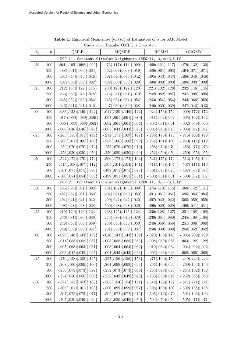
Table 1: Empirical Mean(rmse)[sd]{sd} of Estimators of λ for SAR ModelCases when Regular QMLE is Consistent

λ0 n QMLE MQMLE RGMM ORGMM

DGP 1: Constant Circular Neighbours (REG-1), β0 = (3, 1, 1)′

.50 100 .464 (.105)[.098]{.092} .473(.117)[.114]{.099} .469(.121)[.117] .479(.132)[.130]250 .488(.061)[.060]{.064} .492(.063)[.063]{.059} .489(.064)[.063] .494(.071)[.071]500 .494(.043)[.043]{.046} .497(.043)[.043]{.042} .495(.043)[.043] .498(.048)[.048]

1000 .497(.030)[.030]{.032} .498(.030)[.030]{.029} .498(.030)[.030] .498(.033)[.033].25 100 .212(.133)[.127]{.115} .230(.128)[.127]{.123} .221(.132)[.129] .232(.146)[.145]

250 .233(.080)[.078]{.078} .246(.081)[.081]{.079} .242(.082)[.081] .247(.090)[.090]500 .245(.052)[.052]{.054} .245(.054)[.054]{.054} .243(.054)[.054] .244(.060)[.059]

1000 .246(.041)[.041]{.040} .247(.039)[.039]{.038} .246(.039)[.039] .247(.043)[.043].00 100 -.033(.153)[.149]{.142} -.014(.150)[.149]{.142} -.024(.156)[.154] -.009(.172)[.172]

250 -.017 (.090)[.089]{.089} -.007(.091)[.091]{.089} -.011(.092)[.092] -.005(.102)[.102]500 -.006 (.063)[.063]{.062} -.002(.061)[.061]{.064} -.004(.061)[.061] -.002(.069)[.069]

1000 -.006(.046)[.046]{.046} -.003(.043)[.043]{.045} -.005(.043)[.043] -.003(.047)[.047]-.25 100 -.285(.155)[.151]{.149} -.272(.171)[.169]{.167} -.286(.176)[.173] -.275(.200)[.198]

250 -.266(.101)[.100]{.100} -.258(.100)[.100]{.099} -.264(.101)[.100] -.260(.112)[.112]500 -.259(.070)[.070]{.072} -.255(.070)[.070]{.070} -.258(.070)[.070] -.256(.077)[.076]

1000 -.253(.050)[.050]{.050} -.250(.050)[.050]{.049} -.252(.050)[.050] -.250(.055)[.055]-.50 100 -.524(.172)[.170]{.179} -.506(.172)[.172]{.162} -.521(.175)[.174] -.513(.195)[.194]

250 -.515(.108)[.107]{.112} -.505(.104)[.104]{.101} -.511(.104)[.104] -.507(.117)[.116]500 -.501(.075)[.075]{.080} -.497(.075)[.075]{.073} -.501(.075)[.075] -.497(.084)[.084]

1000 -.500(.054)[.054]{.058} -.499(.051)[.051]{.051} -.500(.051)[.051] -.500(.057)[.057]DGP 2: Constant Circular Neighbours (REG-1), β0 = (3, 1, 1)′

.50 100 .465(.098)[.091]{.093} .481(.107)[.105]{.099} .475(.118)[.115] .488(.142)[.141]250 .487(.062)[.061]{.063} .494(.061)[.060]{.059} .491(.061)[.061] .495(.084)[.084]500 .494(.041)[.041]{.042} .499(.042)[.042]{.040} .497(.042)[.042] .500(.059)[.059]

1000 .498(.028)[.028]{.028} .500(.028)[.028]{.029} .499(.029)[.029] .499(.041)[.041].25 100 .219(.129)[.126]{.124} .238(.125)[.125]{.124} .230(.128)[.127] .251(.168)[.168]

250 .236(.081)[.080]{.080} .243(.080)[.079]{.079} .239(.081)[.080] .245(.108)[.108]500 .246(.056)[.056]{.059} .250(.056)[.056]{.053} .248(.056)[.056] .251(.080)[.080]

1000 .249(.039)[.039]{.041} .251(.039)[.039]{.037} .250(.039)[.039] .250(.052)[.052].00 100 -.029(.146)[.143]{.139} -.010(.143)[.143]{.139} -.020(.150)[.148] -.005(.209)[.209]

250 -.011(.088)[.088]{.087} -.003(.088)[.088]{.085} -.008(.089)[.088] .003(.122)[.122]500 -.005(.063)[.063]{.061} -.008(.064)[.064]{.062} -.010(.064)[.064] -.004(.092)[.092]

1000 -.003(.045)[.045]{.045} -.001(.043)[.043]{.044} -.003(.043)[.043] .000(.060)[.060]-.25 100 -.276(.158)[.155]{.145} -.257(.156)[.156]{.153} -.271(.160)[.159] -.249(.223)[.223]

250 -.268(.100)[.099]{.106} -.261(.099)[.099]{.093} -.266(.100)[.099] -.260(.136)[.136]500 -.256(.073)[.073]{.077} -.252(.073)[.073]{.069} -.255(.074)[.073] -.254(.102)[.102]

1000 -.254(.050)[.050]{.050} -.252(.049)[.049]{.048} -.253(.050)[.049] -.252(.068)[.068]-.50 100 -.527(.155)[.153]{.163} -.505(.154)[.154]{.154} -.519(.158)[.157] -.511(.221)[.221]

250 -.505(.101)[.101]{.103} -.500(.099)[.099]{.097} -.506(.100)[.100] -.502(.138)[.138]500 -.507(.075)[.075]{.077} -.502(.072)[.072]{.072} -.505(.072)[.072] -.501(.103)[.103]

1000 -.505(.050)[.049]{.049} -.503(.050)[.049]{.050} -.504(.050)[.050] -.505(.071)[.071]

26


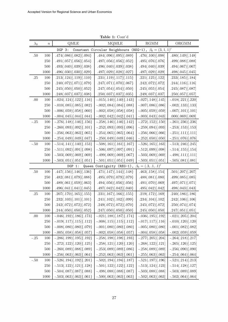
Table 1: Cont’d



.50 100 .474(.086)[.082]{.094} .484(.096)[.095]{.089} .476(.100)[.098] .480(.149)[.148]250 .491(.057)[.056]{.054} .497(.056)[.056]{.052} .495(.076)[.076] .499(.088)[.088]500 .493(.040)[.039]{.038} .496(.040)[.039]{.038} .494(.040)[.039] .494(.067)[.067]

1000 .496(.030)[.030]{.029} .497(.029)[.028]{.027} .497(.029)[.029] .498(.045)[.045].25 100 .213(.124)[.119]{.110} .231(.119)[.117]{.115} .221(.125)[.122] .233(.185)[.184]

250 .240(.072)[.071]{.079} .247(.071)[.070]{.067} .242(.072)[.072] .244(.116)[.116]500 .245(.050)[.050]{.052} .247(.054)[.054]{.050} .245(.055)[.054] .245(.087)[.087]

1000 .248(.037)[.037]{.038} .250(.037)[.037]{.035} .249(.037)[.037] .250(.057)[.057].00 100 -.024(.124)[.122]{.116} -.015(.140)[.140]{.143} -.027(.148)[.145] -.018(.221)[.220]

250 -.010(.085)[.085]{.082} -.002(.084)[.084]{.088} -.007(.086)[.086] -.002(.133)[.133]500 -.006(.059)[.058]{.060} -.002(.058)[.058]{.058} -.005(.059)[.059] -.007(.101)[.101]

1000 -.004(.045)[.044]{.044} -.002(.042)[.042]{.041} -.003(.043)[.043] .000(.069)[.069]-.25 100 -.276(.148)[.146]{.156} -.258(.146)[.146]{.142} -.272(.152)[.150] -.261(.236)[.236]

250 -.260(.093)[.092]{.101} -.252(.093)[.093]{.096} -.259(.094)[.093] -.253(.153)[.153]500 -.256(.063)[.063]{.065} -.254(.065)[.065]{.064} -.256(.066)[.066] -.251(.111)[.111]

1000 -.254(.049)[.049]{.047} -.250(.049)[.049]{.046} -.252(.050)[.050] -.251(.076)[.076]-.50 100 -.514(.141)[.140]{.153} -.508(.161)[.161]{.167} -.526(.165)[.163] -.513(.246)[.245]

250 -.511(.092)[.091]{.098} -.506(.097)[.097]{.091} -.512(.099)[.098] -.514(.155)[.154]500 -.503(.069)[.069]{.069} -.499(.069)[.069]{.067} -.503(.069)[.069] -.498(.111)[.111]

1000 -.503(.051)[.051]{.051} -.501(.051)[.051]{.049} -.503(.051)[.051] -.505(.081)[.081]DGP 1: Queen Contiguity (REG-1), β0 = (.3, .1, .1)′

.50 100 .447(.156)[.146]{.136} .471(.147)[.144]{.148} .463(.158)[.154] .501(.207)[.207]250 .482(.081)[.079]{.088} .495(.079)[.079]{.079} .488(.081)[.080] .499(.085)[.085]500 .489(.061)[.059]{.063} .494(.056)[.056]{.056} .491(.070)[.069] .497(.071)[.071]

1000 .496(.041)[.041]{.045} .497(.042)[.042]{.040} .495(.042)[.042] .498(.043)[.043].25 100 .207(.170)[.165]{.155} .231(.167)[.166]{.155} .219(.172)[.169] .240(.186)[.186]

250 .232(.103)[.101]{.101} .241(.102)[.102]{.099} .234(.104)[.102] .242(.106)[.106]500 .242(.072)[.072]{.072} .249(.072)[.072]{.070} .245(.072)[.072] .250(.074)[.074]

1000 .244(.050)[.050]{.052} .247(.050)[.050]{.050} .245(.050)[.050] .247(.051)[.051].00 100 -.046(.192)[.186]{.173} -.021(.188)[.187]{.174} -.036(.195)[.192] -.021(.205)[.204]

250 -.019(.117)[.115]{.112} -.008(.115)[.115]{.112} -.017(.117)[.116] -.010(.120)[.120]500 -.008(.080)[.080]{.079} -.001(.080)[.080]{.080} -.005(.080)[.080] -.001(.082)[.082]

1000 -.005(.058)[.058]{.057} -.002(.058)[.058]{.057} -.004(.058)[.058] -.002(.059)[.059]-.25 100 -.286(.199)[.195]{.192} -.258(.198)[.198]{.193} -.277(.205)[.204] -.264(.218)[.217]

250 -.272(.122)[.120]{.125} -.258(.121)[.120]{.120} -.268(.122)[.121] -.265(.126)[.125]500 -.260(.089)[.088]{.089} -.253(.089)[.089]{.086} -.258(.089)[.089] -.256(.090)[.090]

1000 -.256(.063)[.063]{.064} -.252(.063)[.063]{.061} -.255(.063)[.063] -.254(.064)[.064]-.50 100 -.526(.194)[.192]{.201} -.502(.194)[.194]{.187} -.521(.197)[.196] -.521(.214)[.213]

250 -.513(.122)[.121]{.128} -.501(.122)[.122]{.122} -.513(.124)[.123] -.514(.128)[.127]500 -.504(.087)[.087]{.088} -.498(.088)[.088]{.087} -.503(.088)[.088] -.503(.089)[.089]

1000 -.503(.063)[.063]{.061} -.500(.063)[.063]{.063} -.502(.063)[.063] -.502(.064)[.064]

27


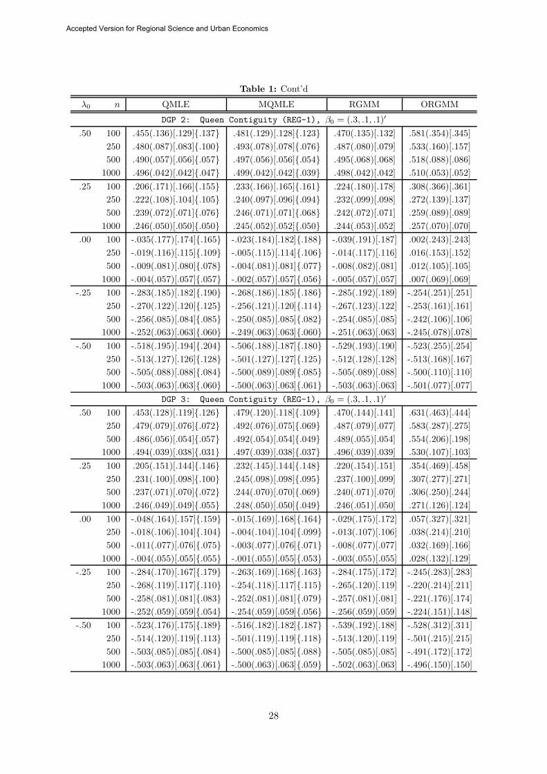
Table 1: Cont’d


DGP 2: Queen Contiguity (REG-1), β0 = (.3, .1, .1)′

.50 100 .455(.136)[.129]{.137} .481(.129)[.128]{.123} .470(.135)[.132] .581(.354)[.345]250 .480(.087)[.083]{.100} .493(.078)[.078]{.076} .487(.080)[.079] .533(.160)[.157]500 .490(.057)[.056]{.057} .497(.056)[.056]{.054} .495(.068)[.068] .518(.088)[.086]

1000 .496(.042)[.042]{.047} .499(.042)[.042]{.039} .498(.042)[.042] .510(.053)[.052].25 100 .206(.171)[.166]{.155} .233(.166)[.165]{.161} .224(.180)[.178] .308(.366)[.361]

250 .222(.108)[.104]{.105} .240(.097)[.096]{.094} .232(.099)[.098] .272(.139)[.137]500 .239(.072)[.071]{.076} .246(.071)[.071]{.068} .242(.072)[.071] .259(.089)[.089]

1000 .246(.050)[.050]{.050} .245(.052)[.052]{.050} .244(.053)[.052] .257(.070)[.070].00 100 -.035(.177)[.174]{.165} -.023(.184)[.182]{.188} -.039(.191)[.187] .002(.243)[.243]

250 -.019(.116)[.115]{.109} -.005(.115)[.114]{.106} -.014(.117)[.116] .016(.153)[.152]500 -.009(.081)[.080]{.078} -.004(.081)[.081]{.077} -.008(.082)[.081] .012(.105)[.105]

1000 -.004(.057)[.057]{.057} -.002(.057)[.057]{.056} -.005(.057)[.057] .007(.069)[.069]-.25 100 -.283(.185)[.182]{.190} -.268(.186)[.185]{.186} -.285(.192)[.189] -.254(.251)[.251]

250 -.270(.122)[.120]{.125} -.256(.121)[.120]{.114} -.267(.123)[.122] -.253(.161)[.161]500 -.256(.085)[.084]{.085} -.250(.085)[.085]{.082} -.254(.085)[.085] -.242(.106)[.106]

1000 -.252(.063)[.063]{.060} -.249(.063)[.063]{.060} -.251(.063)[.063] -.245(.078)[.078]-.50 100 -.518(.195)[.194]{.204} -.506(.188)[.187]{.180} -.529(.193)[.190] -.523(.255)[.254]

250 -.513(.127)[.126]{.128} -.501(.127)[.127]{.125} -.512(.128)[.128] -.513(.168)[.167]500 -.505(.088)[.088]{.084} -.500(.089)[.089]{.085} -.505(.089)[.088] -.500(.110)[.110]

1000 -.503(.063)[.063]{.060} -.500(.063)[.063]{.061} -.503(.063)[.063] -.501(.077)[.077]DGP 3: Queen Contiguity (REG-1), β0 = (.3, .1, .1)′

.50 100 .453(.128)[.119]{.126} .479(.120)[.118]{.109} .470(.144)[.141] .631(.463)[.444]250 .479(.079)[.076]{.072} .492(.076)[.075]{.069} .487(.079)[.077] .583(.287)[.275]500 .486(.056)[.054]{.057} .492(.054)[.054]{.049} .489(.055)[.054] .554(.206)[.198]

1000 .494(.039)[.038]{.031} .497(.039)[.038]{.037} .496(.039)[.039] .530(.107)[.103].25 100 .205(.151)[.144]{.146} .232(.145)[.144]{.148} .220(.154)[.151] .354(.469)[.458]

250 .231(.100)[.098]{.100} .245(.098)[.098]{.095} .237(.100)[.099] .307(.277)[.271]500 .237(.071)[.070]{.072} .244(.070)[.070]{.069} .240(.071)[.070] .306(.250)[.244]

1000 .246(.049)[.049]{.055} .248(.050)[.050]{.049} .246(.051)[.050] .271(.126)[.124].00 100 -.048(.164)[.157]{.159} -.015(.169)[.168]{.164} -.029(.175)[.172] .057(.327)[.321]

250 -.018(.106)[.104]{.104} -.004(.104)[.104]{.099} -.013(.107)[.106] .038(.214)[.210]500 -.011(.077)[.076]{.075} -.003(.077)[.076]{.071} -.008(.077)[.077] .032(.169)[.166]

1000 -.004(.055)[.055]{.055} -.001(.055)[.055]{.053} -.003(.055)[.055] .028(.132)[.129]-.25 100 -.284(.170)[.167]{.179} -.263(.169)[.168]{.163} -.284(.175)[.172] -.245(.283)[.283]

250 -.268(.119)[.117]{.110} -.254(.118)[.117]{.115} -.265(.120)[.119] -.220(.214)[.211]500 -.258(.081)[.081]{.083} -.252(.081)[.081]{.079} -.257(.081)[.081] -.221(.176)[.174]

1000 -.252(.059)[.059]{.054} -.254(.059)[.059]{.056} -.256(.059)[.059] -.224(.151)[.148]-.50 100 -.523(.176)[.175]{.189} -.516(.182)[.182]{.187} -.539(.192)[.188] -.528(.312)[.311]

250 -.514(.120)[.119]{.113} -.501(.119)[.119]{.118} -.513(.120)[.119] -.501(.215)[.215]500 -.503(.085)[.085]{.084} -.500(.085)[.085]{.088} -.505(.085)[.085] -.491(.172)[.172]

1000 -.503(.063)[.063]{.061} -.500(.063)[.063]{.059} -.502(.063)[.063] -.496(.150)[.150]

28


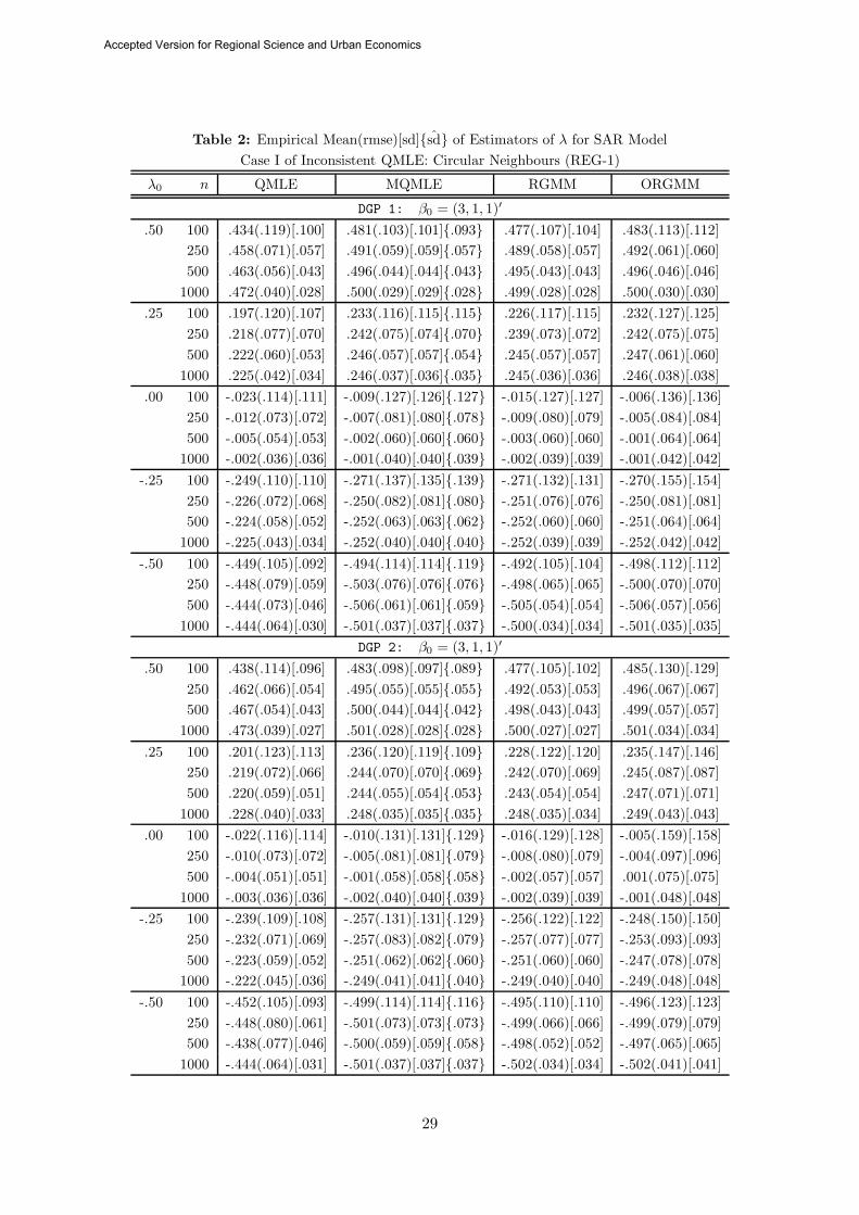
Table 2: Empirical Mean(rmse)[sd]{sd} of Estimators of λ for SAR ModelCase I of Inconsistent QMLE: Circular Neighbours (REG-1)


DGP 1: β0 = (3, 1, 1)′

.50 100 .434(.119)[.100] .481(.103)[.101]{.093} .477(.107)[.104] .483(.113)[.112]250 .458(.071)[.057] .491(.059)[.059]{.057} .489(.058)[.057] .492(.061)[.060]500 .463(.056)[.043] .496(.044)[.044]{.043} .495(.043)[.043] .496(.046)[.046]

1000 .472(.040)[.028] .500(.029)[.029]{.028} .499(.028)[.028] .500(.030)[.030].25 100 .197(.120)[.107] .233(.116)[.115]{.115} .226(.117)[.115] .232(.127)[.125]

250 .218(.077)[.070] .242(.075)[.074]{.070} .239(.073)[.072] .242(.075)[.075]500 .222(.060)[.053] .246(.057)[.057]{.054} .245(.057)[.057] .247(.061)[.060]

1000 .225(.042)[.034] .246(.037)[.036]{.035} .245(.036)[.036] .246(.038)[.038].00 100 -.023(.114)[.111] -.009(.127)[.126]{.127} -.015(.127)[.127] -.006(.136)[.136]

250 -.012(.073)[.072] -.007(.081)[.080]{.078} -.009(.080)[.079] -.005(.084)[.084]500 -.005(.054)[.053] -.002(.060)[.060]{.060} -.003(.060)[.060] -.001(.064)[.064]

1000 -.002(.036)[.036] -.001(.040)[.040]{.039} -.002(.039)[.039] -.001(.042)[.042]-.25 100 -.249(.110)[.110] -.271(.137)[.135]{.139} -.271(.132)[.131] -.270(.155)[.154]

250 -.226(.072)[.068] -.250(.082)[.081]{.080} -.251(.076)[.076] -.250(.081)[.081]500 -.224(.058)[.052] -.252(.063)[.063]{.062} -.252(.060)[.060] -.251(.064)[.064]

1000 -.225(.043)[.034] -.252(.040)[.040]{.040} -.252(.039)[.039] -.252(.042)[.042]-.50 100 -.449(.105)[.092] -.494(.114)[.114]{.119} -.492(.105)[.104] -.498(.112)[.112]

250 -.448(.079)[.059] -.503(.076)[.076]{.076} -.498(.065)[.065] -.500(.070)[.070]500 -.444(.073)[.046] -.506(.061)[.061]{.059} -.505(.054)[.054] -.506(.057)[.056]

1000 -.444(.064)[.030] -.501(.037)[.037]{.037} -.500(.034)[.034] -.501(.035)[.035]DGP 2: β0 = (3, 1, 1)′

.50 100 .438(.114)[.096] .483(.098)[.097]{.089} .477(.105)[.102] .485(.130)[.129]250 .462(.066)[.054] .495(.055)[.055]{.055} .492(.053)[.053] .496(.067)[.067]500 .467(.054)[.043] .500(.044)[.044]{.042} .498(.043)[.043] .499(.057)[.057]

1000 .473(.039)[.027] .501(.028)[.028]{.028} .500(.027)[.027] .501(.034)[.034].25 100 .201(.123)[.113] .236(.120)[.119]{.109} .228(.122)[.120] .235(.147)[.146]

250 .219(.072)[.066] .244(.070)[.070]{.069} .242(.070)[.069] .245(.087)[.087]500 .220(.059)[.051] .244(.055)[.054]{.053} .243(.054)[.054] .247(.071)[.071]

1000 .228(.040)[.033] .248(.035)[.035]{.035} .248(.035)[.034] .249(.043)[.043].00 100 -.022(.116)[.114] -.010(.131)[.131]{.129} -.016(.129)[.128] -.005(.159)[.158]

250 -.010(.073)[.072] -.005(.081)[.081]{.079} -.008(.080)[.079] -.004(.097)[.096]500 -.004(.051)[.051] -.001(.058)[.058]{.058} -.002(.057)[.057] .001(.075)[.075]

1000 -.003(.036)[.036] -.002(.040)[.040]{.039} -.002(.039)[.039] -.001(.048)[.048]-.25 100 -.239(.109)[.108] -.257(.131)[.131]{.129} -.256(.122)[.122] -.248(.150)[.150]

250 -.232(.071)[.069] -.257(.083)[.082]{.079} -.257(.077)[.077] -.253(.093)[.093]500 -.223(.059)[.052] -.251(.062)[.062]{.060} -.251(.060)[.060] -.247(.078)[.078]

1000 -.222(.045)[.036] -.249(.041)[.041]{.040} -.249(.040)[.040] -.249(.048)[.048]-.50 100 -.452(.105)[.093] -.499(.114)[.114]{.116} -.495(.110)[.110] -.496(.123)[.123]

250 -.448(.080)[.061] -.501(.073)[.073]{.073} -.499(.066)[.066] -.499(.079)[.079]500 -.438(.077)[.046] -.500(.059)[.059]{.058} -.498(.052)[.052] -.497(.065)[.065]

1000 -.444(.064)[.031] -.501(.037)[.037]{.037} -.502(.034)[.034] -.502(.041)[.041]

29


Table 2: Cont’d


DGP 3: β0 = (3, 1, 1)′

.50 100 .445(.107)[.092] .486(.087)[.086]{.079} .482(.092)[.090] .493(.144)[.144]250 .464(.066)[.055] .495(.054)[.054]{.049} .493(.054)[.053] .497(.073)[.073]500 .467(.055)[.044] .497(.041)[.041]{.039} .496(.042)[.041] .497(.060)[.060]

1000 .473(.040)[.030] .499(.027)[.027]{.026} .499(.027)[.027] .500(.037)[.037].25 100 .199(.116)[.105] .230(.110)[.108]{.099} .241(.068)[.067] .245(.090)[.089]

250 .219(.071)[.064] .243(.069)[.068]{.063} .241(.068)[.067] .245(.090)[.089]500 .222(.058)[.050] .244(.054)[.053]{.049} .243(.053)[.053] .242(.078)[.078]

1000 .228(.040)[.033] .248(.035)[.034]{.033} .248(.034)[.034] .250(.045)[.045].00 100 -.019(.107)[.105] -.008(.120)[.120]{.119} -.013(.119)[.119] -.005(.164)[.164]

250 -.008(.065)[.065] -.003(.072)[.072]{.069} -.006(.072)[.072] -.003(.101)[.101]500 -.006(.051)[.050] -.004(.057)[.057]{.054} -.006(.058)[.058] -.007(.089)[.089]

1000 -.003(.035)[.034] -.002(.038)[.038]{.037} -.003(.038)[.038] -.003(.053)[.053]-.25 100 -.243(.102)[.102] -.260(.123)[.123]{.120} -.262(.118)[.117] -.257(.157)[.156]

250 -.230(.072)[.069] -.250(.077)[.077]{.072} -.251(.074)[.074] -.248(.098)[.098]500 -.228(.055)[.050] -.255(.058)[.058]{.056} -.256(.058)[.057] -.255(.083)[.083]

1000 -.223(.044)[.035] -.250(.039)[.039]{.038} -.250(.039)[.039] -.249(.052)[.052]-.50 100 -.450(.107)[.095] -.486(.110)[.109]{.112} -.485(.105)[.104] -.484(.125)[.123]

250 -.450(.081)[.063] -.502(.074)[.074]{.070} -.498(.064)[.064] -.496(.085)[.085]500 -.439(.081)[.053] -.499(.061)[.061]{.059} -.497(.051)[.051] -.499(.069)[.069]

1000 -.445(.066)[.037] -.500(.038)[.038]{.036} -.500(.034)[.034] -.501(.044)[.044]DGP 1: β0 = (.3, .1, .1)′

.50 100 .407(.154)[.123] .474(.129)[.127]{.119} .467(.148)[.144] .499(.189)[.189]250 .437(.100)[.078] .489(.080)[.079]{.075} .485(.082)[.080] .494(.083)[.083]500 .445(.076)[.053] .494(.054)[.054]{.053} .493(.069)[.069] .497(.066)[.066]

1000 .453(.060)[.037] .499(.037)[.037]{.038} .498(.037)[.037] .500(.038)[.038].25 100 .174(.156)[.136] .226(.155)[.153]{.149} .213(.165)[.161] .235(.195)[.194]

250 .199(.101)[.087] .238(.097)[.097]{.096} .233(.100)[.098] .241(.102)[.102]500 .208(.076)[.063] .243(.069)[.069]{.068} .240(.070)[.069] .243(.070)[.070]

1000 .213(.058)[.045] .246(.049)[.049]{.048} .245(.050)[.049] .246(.050)[.050].00 100 -.041(.146)[.140] -.023(.170)[.168]{.165} -.040(.179)[.174] -.026(.184)[.182]

250 -.016(.096)[.095] -.009(.114)[.113]{.117} -.015(.115)[.114] -.009(.116)[.116]500 -.008(.066)[.066] -.004(.078)[.078]{.077} -.008(.079)[.079] -.005(.080)[.080]

1000 -.004(.044)[.044] -.002(.052)[.052]{.054} -.003(.052)[.052] -.002(.053)[.053]-.25 100 -.240(.136)[.136] -.270(.176)[.175]{.172} -.292(.185)[.180] -.291(.201)[.197]

250 -.213(.095)[.087] -.251(.110)[.110]{.111} -.259(.111)[.111] -.256(.114)[.114]500 -.210(.074)[.062] -.252(.079)[.079]{.079} -.256(.079)[.079] -.255(.080)[080]

1000 -.209(.060)[.044] -.252(.055)[.055]{.056} -.254(.055)[.055] -.254(.056)[.056]-.50 100 -.417(.149)[.124] -.496(.164)[.164]{.159} -.531(.202)[.199] -.535(.213)[.210]

250 -.413(.117)[.078] -.504(.103)[.103]{.102} -.512(.103)[.102] -.516(.107)[.106]500 -.409(.107)[.056] -.501(.073)[.073]{.073} -.506(.073)[.073] -.507(.074)[.074]

1000 -.405(.103)[.039] -.498(.051)[.051]{.052} -.501(.051)[.051] -.501(.051)[.051]

30


Table 2: Cont’d


DGP 2: β0 = (.3, .1, .1)′

.50 100 .416(.147)[.121] .482(.123)[.121]{.119} .475(.138)[.136] .592(.342)[.329]250 .438(.101)[.080] .490(.081)[.080]{.079} .487(.090)[.089] .528(.157)[.154]500 .448(.074)[.053] .496(.053)[.053]{.052} .494(.054)[.053] .511(.068)[.067]

1000 .452(.061)[.038] .499(.038)[.038]{.037} .498(.038)[.038] .508(.047)[.047].25 100 .184(.152)[.137] .236(.154)[.154]{.157} .224(.165)[.163] .304(.305)[.301]

250 .203(.100)[.088] .242(.097)[.097]{.091} .236(.099)[.098] .271(.149)[.147]500 .211(.073)[.062] .246(.067)[.067]{.066} .243(.068)[.068] .264(.109)[.109]

1000 .217(.055)[.044] .250(.048)[.048]{.047} .249(.048)[.048] .258(.058)[.058].00 100 -.040(.144)[.139] -.021(.171)[.169]{.164} -.039(.180)[.176] .014(.262)[.262]

250 -.016(.091)[.089] -.010(.107)[.107]{.104} -.016(.109)[.108] .008(.134)[.134]500 -.007(.063)[.063] -.003(.075)[.075]{.074} -.006(.075)[.075] .008(.090)[.090]

1000 -.003(.046)[.046] -.001(.054)[.054]{.053} -.003(.054)[.054] .006(.066)[.066]-.25 100 -.232(.133)[.131] -.259(.169)[.169]{.159} -.281(.180)[.177] -.254(.266)[.266]

250 -.216(.090)[.083] -.254(.106)[.106]{.107} -.262(.108)[.107] -.249(.138)[.138]500 -.210(.073)[.061] -.251(.077)[.077]{.077} -.255(.077)[.077] -.246(.088)[.088]

1000 -.207(.063)[.046] -.249(.057)[.057]{.055} -.251(.057)[.057] -.247(.067)[.067]-.50 100 -.424(.148)[.127] -.503(.163)[.163]{.160} -.535(.191)[.187] -.549(.246)[.241]

250 -.410(.123)[.084] -.499(.105)[.105]{.099} -.507(.106)[.105] -.513(.151)[.151]500 -.409(.108)[.058] -.500(.071)[.071]{.072} -.504(.071)[.071] -.507(.086)[.086]

1000 -.409(.100)[.041] -.503(.050)[.050]{.051} -.506(.051)[.050] -.509(.063)[.062]DGP 3: β0 = (.3, .1, .1)′

.50 100 .416(.147)[.120] .480(.118)[.116]{.099} .473(.130)[.128] .652(.453)[.426]250 .439(.096)[.074] .490(.071)[.070]{.065} .486(.073)[.071] .572(.247)[.236]500 .449(.074)[.054] .497(.050)[.050]{.048} .495(.051)[.051] .547(.189)[.184]

1000 .453(.060)[.037] .498(.034)[.034]{.035} .497(.035)[.034] .523(.104)[.101].25 100 .174(.153)[.133] .224(.147)[.144]{.137} .212(.156)[.152] .335(.387)[.378]

250 .210(.089)[.080] .249(.087)[.087]{.083} .243(.087)[.087] .310(.245)[.237]500 .211(.072)[.061] .244(.065)[.065]{.061} .242(.066)[.065] .283(.198)[.195]

1000 .214(.057)[.044] .247(.046)[.046]{.044} .246(.047)[.046] .266(.116)[.115].00 100 -.027(.135)[.133] -.008(.161)[.160]{.153} -.026(.172)[.170] .077(.422)[.414]

250 -.014(.087)[.086] -.006(.103)[.103]{.099} -.013(.105)[.104] .052(.263)[.258]500 -.008(.059)[.058] -.004(.070)[.070]{.069} -.008(.071)[.070] .026(.151)[.149]

1000 -.003(.042)[.042] -.001(.050)[.050]{.050} -.003(.050)[.050] .025(.116)[.114]-.25 100 -.234(.131)[.130] -.262(.172)[.172]{.179} -.288(.184)[.180] -.238(.295)[.295]

250 -.218(.090)[.084] -.254(.105)[.105]{.099} -.262(.107)[.106] -.223(.239)[.238]500 -.213(.073)[.063] -.252(.076)[.076]{.071} -.256(.077)[.076] -.233(.161)[.160]

1000 -.208(.062)[.046] -.250(.055)[.055]{.053} -.252(.055)[.055] -.238(.128)[.127]-.50 100 -.418(.151)[.127] -.495(.158)[.158]{.151} -.526(.178)[.176] -.544(.304)[.301]

250 -.411(.126)[.089] -.503(.105)[.105]{.099} -.511(.105)[.104] -.508(.199)[.198]500 -.408(.113)[.066] -.500(.073)[.073]{.069} -.504(.072)[.072] -.501(.156)[.156]

1000 -.403(.109)[.049] -.496(.051)[.051]{.049} -.498(.051)[.051] -.502(.129)[.129]

31


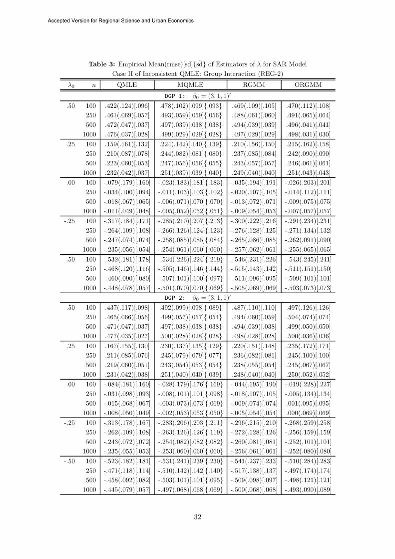
Table 3: Empirical Mean(rmse)[sd]{sd} of Estimators of λ for SAR ModelCase II of Inconsistent QMLE: Group Interaction (REG-2)


DGP 1: β0 = (3, 1, 1)′

.50 100 .422(.124)[.096] .478(.102)[.099]{.093} .469(.109)[.105] .470(.112)[.108]250 .461(.069)[.057] .493(.059)[.059]{.056} .488(.061)[.060] .491(.065)[.064]500 .472(.047)[.037] .497(.039)[.038]{.038} .494(.039)[.039] .496(.041)[.041]

1000 .476(.037)[.028] .499(.029)[.029]{.028} .497(.029)[.029] .498(.031)[.030].25 100 .159(.161)[.132] .224(.142)[.140]{.139} .210(.156)[.150] .215(.162)[.158]

250 .210(.087)[.078] .244(.082)[.081]{.080} .237(.085)[.084] .242(.090)[.090]500 .223(.060)[.053] .247(.056)[.056]{.055} .243(.057)[.057] .246(.061)[.061]

1000 .232(.042)[.037] .251(.039)[.039]{.040} .249(.040)[.040] .251(.043)[.043].00 100 -.079(.179)[.160] -.023(.183)[.181]{.183} -.035(.194)[.191] -.026(.203)[.201]

250 -.034(.100)[.094] -.011(.103)[.103]{.102} -.020(.107)[.105] -.014(.112)[.111]500 -.018(.067)[.065] -.006(.071)[.070]{.070} -.013(.072)[.071] -.009(.075)[.075]

1000 -.011(.049)[.048] -.005(.052)[.052]{.051} -.009(.054)[.053] -.007(.057)[.057]-.25 100 -.317(.184)[.171] -.285(.210)[.207]{.213} -.300(.222)[.216] -.291(.234)[.231]

250 -.264(.109)[.108] -.266(.126)[.124]{.123} -.276(.128)[.125] -.271(.134)[.132]500 -.247(.074)[.074] -.258(.085)[.085]{.084} -.265(.086)[.085] -.262(.091)[.090]

1000 -.235(.056)[.054] -.254(.061)[.060]{.060} -.257(.062)[.061] -.255(.065)[.065]-.50 100 -.532(.181)[.178] -.534(.226)[.224]{.219} -.546(.231)[.226] -.543(.245)[.241]

250 -.468(.120)[.116] -.505(.146)[.146]{.144} -.515(.143)[.142] -.511(.151)[.150]500 -.460(.090)[.080] -.507(.101)[.100]{.097} -.511(.096)[.095] -.509(.101)[.101]

1000 -.448(.078)[.057] -.501(.070)[.070]{.069} -.505(.069)[.069] -.503(.073)[.073]DGP 2: β0 = (3, 1, 1)′

.50 100 .437(.117)[.098] .492(.099)[.098]{.089} .487(.110)[.110] .497(.126)[.126]250 .465(.066)[.056] .499(.057)[.057]{.054} .494(.060)[.059] .504(.074)[.074]500 .471(.047)[.037] .497(.038)[.038]{.038} .494(.039)[.038] .499(.050)[.050]

1000 .477(.035)[.027] .500(.028)[.028]{.028} .498(.028)[.028] .500(.036)[.036].25 100 .167(.155)[.130] .230(.137)[.135]{.129} .220(.151)[.148] .235(.172)[.171]

250 .211(.085)[.076] .245(.079)[.079]{.077} .236(.082)[.081] .245(.100)[.100]500 .219(.060)[.051] .243(.054)[.053]{.054} .238(.055)[.054] .245(.067)[.067]

1000 .231(.042)[.038] .251(.040)[.040]{.039} .248(.040)[.040] .250(.052)[.052].00 100 -.084(.181)[.160] -.028(.179)[.176]{.169} -.044(.195)[.190] -.019(.228)[.227]

250 -.031(.098)[.093] -.008(.101)[.101]{.098} -.018(.107)[.105] -.005(.134)[.134]500 -.015(.068)[.067] -.003(.073)[.073]{.069} -.009(.074)[.074] .001(.095)[.095]

1000 -.008(.050)[.049] -.002(.053)[.053]{.050} -.005(.054)[.054] .000(.069)[.069]-.25 100 -.313(.178)[.167] -.283(.206)[.203]{.211} -.296(.215)[.210] -.268(.259)[.258]

250 -.262(.109)[.108] -.263(.126)[.126]{.119} -.272(.128)[.126] -.256(.159)[.159]500 -.243(.072)[.072] -.254(.082)[.082]{.082} -.260(.081)[.081] -.252(.101)[.101]

1000 -.235(.055)[.053] -.253(.060)[.060]{.060} -.256(.061)[.061] -.252(.080)[.080]-.50 100 -.523(.182)[.181] -.531(.241)[.239]{.230} -.541(.237)[.233] -.510(.284)[.283]

250 -.471(.118)[.114] -.510(.142)[.142]{.140} -.517(.138)[.137] -.497(.174)[.174]500 -.458(.092)[.082] -.503(.101)[.101]{.095} -.509(.098)[.097] -.498(.121)[.121]

1000 -.445(.079)[.057] -.497(.068)[.068]{.069} -.500(.068)[.068] -.493(.090)[.089]

32


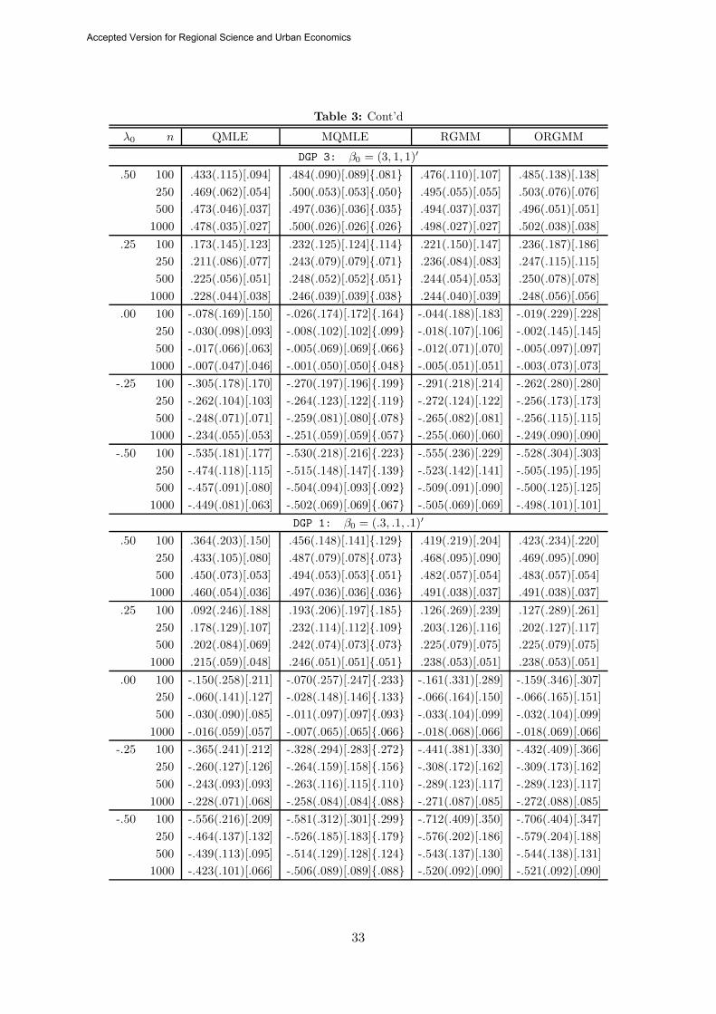
Table 3: Cont’d


DGP 3: β0 = (3, 1, 1)′

.50 100 .433(.115)[.094] .484(.090)[.089]{.081} .476(.110)[.107] .485(.138)[.138]250 .469(.062)[.054] .500(.053)[.053]{.050} .495(.055)[.055] .503(.076)[.076]500 .473(.046)[.037] .497(.036)[.036]{.035} .494(.037)[.037] .496(.051)[.051]

1000 .478(.035)[.027] .500(.026)[.026]{.026} .498(.027)[.027] .502(.038)[.038].25 100 .173(.145)[.123] .232(.125)[.124]{.114} .221(.150)[.147] .236(.187)[.186]

250 .211(.086)[.077] .243(.079)[.079]{.071} .236(.084)[.083] .247(.115)[.115]500 .225(.056)[.051] .248(.052)[.052]{.051} .244(.054)[.053] .250(.078)[.078]

1000 .228(.044)[.038] .246(.039)[.039]{.038} .244(.040)[.039] .248(.056)[.056].00 100 -.078(.169)[.150] -.026(.174)[.172]{.164} -.044(.188)[.183] -.019(.229)[.228]

250 -.030(.098)[.093] -.008(.102)[.102]{.099} -.018(.107)[.106] -.002(.145)[.145]500 -.017(.066)[.063] -.005(.069)[.069]{.066} -.012(.071)[.070] -.005(.097)[.097]

1000 -.007(.047)[.046] -.001(.050)[.050]{.048} -.005(.051)[.051] -.003(.073)[.073]-.25 100 -.305(.178)[.170] -.270(.197)[.196]{.199} -.291(.218)[.214] -.262(.280)[.280]

250 -.262(.104)[.103] -.264(.123)[.122]{.119} -.272(.124)[.122] -.256(.173)[.173]500 -.248(.071)[.071] -.259(.081)[.080]{.078} -.265(.082)[.081] -.256(.115)[.115]

1000 -.234(.055)[.053] -.251(.059)[.059]{.057} -.255(.060)[.060] -.249(.090)[.090]-.50 100 -.535(.181)[.177] -.530(.218)[.216]{.223} -.555(.236)[.229] -.528(.304)[.303]

250 -.474(.118)[.115] -.515(.148)[.147]{.139} -.523(.142)[.141] -.505(.195)[.195]500 -.457(.091)[.080] -.504(.094)[.093]{.092} -.509(.091)[.090] -.500(.125)[.125]

1000 -.449(.081)[.063] -.502(.069)[.069]{.067} -.505(.069)[.069] -.498(.101)[.101]DGP 1: β0 = (.3, .1, .1)′

.50 100 .364(.203)[.150] .456(.148)[.141]{.129} .419(.219)[.204] .423(.234)[.220]250 .433(.105)[.080] .487(.079)[.078]{.073} .468(.095)[.090] .469(.095)[.090]500 .450(.073)[.053] .494(.053)[.053]{.051} .482(.057)[.054] .483(.057)[.054]

1000 .460(.054)[.036] .497(.036)[.036]{.036} .491(.038)[.037] .491(.038)[.037].25 100 .092(.246)[.188] .193(.206)[.197]{.185} .126(.269)[.239] .127(.289)[.261]

250 .178(.129)[.107] .232(.114)[.112]{.109} .203(.126)[.116] .202(.127)[.117]500 .202(.084)[.069] .242(.074)[.073]{.073} .225(.079)[.075] .225(.079)[.075]

1000 .215(.059)[.048] .246(.051)[.051]{.051} .238(.053)[.051] .238(.053)[.051].00 100 -.150(.258)[.211] -.070(.257)[.247]{.233} -.161(.331)[.289] -.159(.346)[.307]

250 -.060(.141)[.127] -.028(.148)[.146]{.133} -.066(.164)[.150] -.066(.165)[.151]500 -.030(.090)[.085] -.011(.097)[.097]{.093} -.033(.104)[.099] -.032(.104)[.099]

1000 -.016(.059)[.057] -.007(.065)[.065]{.066} -.018(.068)[.066] -.018(.069)[.066]-.25 100 -.365(.241)[.212] -.328(.294)[.283]{.272} -.441(.381)[.330] -.432(.409)[.366]

250 -.260(.127)[.126] -.264(.159)[.158]{.156} -.308(.172)[.162] -.309(.173)[.162]500 -.243(.093)[.093] -.263(.116)[.115]{.110} -.289(.123)[.117] -.289(.123)[.117]

1000 -.228(.071)[.068] -.258(.084)[.084]{.088} -.271(.087)[.085] -.272(.088)[.085]-.50 100 -.556(.216)[.209] -.581(.312)[.301]{.299} -.712(.409)[.350] -.706(.404)[.347]

250 -.464(.137)[.132] -.526(.185)[.183]{.179} -.576(.202)[.186] -.579(.204)[.188]500 -.439(.113)[.095] -.514(.129)[.128]{.124} -.543(.137)[.130] -.544(.138)[.131]

1000 -.423(.101)[.066] -.506(.089)[.089]{.088} -.520(.092)[.090] -.521(.092)[.090]

33


Table 3: Cont’d


DGP 2: β0 = (.3, .1, .1)′

.50 100 .361(.206)[.152] .453(.150)[.143]{.137} .426(.251)[.240] .518(.396)[.396]250 .435(.103)[.080] .489(.078)[.077]{.070} .469(.085)[.079] .510(.185)[.185]500 .453(.070)[.052] .496(.050)[.050]{.049} .485(.053)[.051] .502(.113)[.113]

1000 .460(.054)[.037] .497(.036)[.036]{.035} .492(.038)[.037] .494(.042)[.042].25 100 .098(.241)[.187] .197(.202)[.194]{.186} .134(.269)[.242] .230(.459)[.459]

250 .176(.131)[.108] .229(.116)[.114]{.109} .199(.128)[.117] .231(.219)[.218]500 .200(.086)[.070] .239(.075)[.074]{.071} .222(.080)[.075] .234(.113)[.112]

1000 .215(.062)[.052] .246(.055)[.055]{.051} .238(.057)[.055] .239(.062)[.061].00 100 -.144(.254)[.209] -.064(.257)[.249]{.241} -.154(.314)[.273] -.029(.573)[.573]

250 -.052(.127)[.116] -.017(.132)[.131]{.129} -.054(.146)[.136] -.015(.267)[.266]500 -.032(.091)[.085] -.014(.098)[.097]{.090} -.036(.105)[.099] -.024(.119)[.116]

1000 -.018(.063)[.060] -.009(.069)[.069]{.065} -.020(.072)[.069] -.014(.082)[.081]-.25 100 -.354(.235)[.211] -.311(.283)[.276]{.265} -.423(.348)[.302] -.320(.534)[.529]

250 -.264(.131)[.130] -.268(.164)[.163]{.159} -.312(.180)[.168] -.278(.271)[.269]500 -.241(.090)[.089] -.260(.110)[.109]{.106} -.286(.117)[.111] -.269(.136)[.135]

1000 -.228(.067)[.064] -.257(.078)[.078]{.077} -.270(.081)[.078] -.266(.092)[.091]-.50 100 -.543(.218)[.214] -.559(.308)[.302]{.296} -.696(.424)[.376] -.621(.616)[.604]

250 -.468(.138)[.135] -.532(.186)[.183]{.179} -.583(.203)[.186] -.563(.248)[.240]500 -.444(.113)[.098] -.520(.129)[.128]{.122} -.549(.138)[.129] -.538(.161)[.156]

1000 -.420(.104)[.066] -.503(.086)[.086]{.087} -.517(.088)[.086] -.512(.101)[.100]DGP 3: β0 = (.3, .1, .1)′

.50 100 .378(.186)[.140] .470(.131)[.127]{.114} .439(.225)[.217] .575(.428)[.421]250 .434(.100)[.076] .487(.071)[.070]{.074} .467(.080)[.073] .536(.255)[.253]500 .450(.074)[.055] .492(.052)[.051]{.049} .481(.056)[.052] .539(.229)[.226]

1000 .460(.055)[.037] .497(.035)[.035]{.033} .491(.036)[.035] .523(.168)[.167].25 100 .109(.217)[.165] .210(.173)[.168]{.160} .151(.252)[.232] .286(.518)[.517]

250 .183(.120)[.099] .235(.103)[.102]{.099} .207(.114)[.106] .310(.398)[.394]500 .205(.081)[.067] .243(.069)[.069]{.066} .227(.074)[.070] .287(.286)[.284]

1000 .215(.058)[.046] .246(.048)[.048]{.047} .237(.050)[.048] .265(.179)[.179].00 100 -.144(.241)[.194] -.063(.235)[.227]{.199} -.144(.329)[.296] .056(.696)[.694]

250 -.051(.123)[.112] -.018(.130)[.129]{.119} -.054(.144)[.133] .094(.551)[.543]500 -.027(.084)[.079] -.008(.091)[.090]{.089} -.030(.098)[.093] .032(.337)[.336]

1000 -.015(.058)[.056] -.006(.065)[.064]{.061} -.017(.067)[.065] .020(.210)[.209]-.25 100 -.355(.231)[.205] -.313(.273)[.265]{.250} -.432(.357)[.307] -.193(.780)[.778]

250 -.267(.129)[.128] -.272(.162)[.160]{.151} -.317(.180)[.167] -.183(.540)[.536]500 -.240(.087)[.086] -.259(.106)[.106]{.100} -.285(.114)[.108] -.202(.376)[.373]

1000 -.224(.068)[.063] -.254(.075)[.075]{.073} -.267(.078)[.076] -.213(.253)[.251]-.50 100 -.544(.209)[.204] -.557(.290)[.284]{.279} -.684(.447)[.407] -.442(.904)[.903]

250 -.467(.139)[.135] -.526(.179)[.177]{.168} -.577(.196)[.180] -.464(.523)[.522]500 -.433(.119)[.099] -.506(.123)[.123]{.119} -.535(.130)[.125] -.412(.483)[.475]

1000 -.423(.107)[.074] -.504(.086)[.086]{.083} -.519(.088)[.086] -.466(.257)[.255]

34


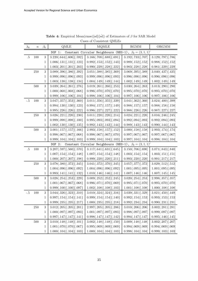
Table 4: Empirical Mean(rmse)[sd]{sd} of Estimators of β for SAR ModelCases of Consistent QMLEs

λ0 n β0 QMLE MQMLE RGMM ORGMM


.5 100 3 3.220(.644)[.606]{.592} 3.166(.708)[.688]{.691} 3.192(.733)[.707] 3.129(.797)[.786]1 1.006(.131)[.131]{.123} 0.992(.153)[.152]{.143} 0.989(.152)[.152] 0.988(.152)[.152]1 1.003(.201)[.201]{.203} 0.990(.229)[.228]{.222} 0.983(.228)[.228] 0.981(.229)[.229]

250 3 3.089(.396)[.386]{.392} 3.051(.388)[.385]{.369} 3.069(.395)[.389] 3.040(.437)[.435]1 0.999(.096)[.096]{.093} 0.999(.096)[.096]{.093} 0.996(.096)[.096] 0.996(.096)[.096]1 1.003(.138)[.138]{.134} 1.004(.149)[.149]{.144} 1.002(.149)[.149] 1.002(.149)[.149]

500 3 3.039(.264)[.261]{.276} 3.019(.261)[.260]{.253} 3.030(.264)[.263] 3.013(.290)[.290]1 1.000(.068)[.068]{.068} 0.996(.070)[.070]{.070} 0.995(.070)[.070] 0.995(.070)[.070]1 0.999(.106)[.106]{.104} 0.998(.106)[.106]{.104} 0.997(.106)[.106] 0.997(.106)[.106]

-.5 100 3 3.047(.357)[.353]{.360} 3.011(.356)[.355]{.339} 3.041(.362)[.360] 3.024(.400)[.399]1 0.994(.130)[.130]{.123} 0.994(.157)[.157]{.149} 0.988(.157)[.157] 0.988(.158)[.158]1 0.995(.226)[.226]{.222} 0.996(.227)[.227]{.222} 0.988(.226)[.226] 0.987(.227)[.227]

250 3 3.026(.221)[.220]{.230} 3.011(.220)[.220]{.214} 3.024(.221)[.220] 3.016(.246)[.245]1 0.999(.098)[.098]{.100} 0.995(.093)[.093]{.094} 0.992(.094)[.093] 0.992(.094)[.093]1 1.002(.130)[.130]{.135} 0.992(.143)[.143]{.144} 0.989(.143)[.143] 0.990(.144)[.143]

500 3 3.001(.157)[.157]{.166} 2.993(.158)[.157]{.152} 3.000(.158)[.158] 2.993(.174)[.174]1 0.998(.067)[.067]{.068} 0.998(.067)[.067]{.070} 0.997(.067)[.067] 0.997(.067)[.067]1 0.999(.104)[.104]{.103} 0.999(.104)[.104]{.103} 0.997(.104)[.104] 0.998(.104)[.104]


.5 100 3 3.207(.597)[.560]{.570} 3.117(.641)[.631]{.645} 3.150(.706)[.690] 3.071(.843)[.840]1 1.007(.154)[.154]{.148} 1.007(.154)[.154]{.148} 1.003(.154)[.154] 1.003(.151)[.151]1 1.000(.207)[.207]{.198} 0.999(.220)[.220]{.211} 0.993(.220)[.220] 0.991(.217)[.217]

250 3 3.078(.380)[.372]{.345} 3.041(.372)[.370]{.345} 3.057(.377)[.372] 3.029(.512)[.512]1 1.004(.096)[.096]{.092} 1.004(.096)[.096]{.092} 1.001(.095)[.095] 1.001(.095)[.095]1 0.993(.141)[.141]{.132} 1.010(.146)[.146]{.141} 1.007(.146)[.146] 1.007(.145)[.145]

500 3 3.028(.254)[.253]{.229} 3.009(.252)[.252]{.245} 3.020(.254)[.253] 2.998(.357)[.357]1 1.001(.067)[.067]{.068} 0.996(.071)[.070]{.069} 0.995(.071)[.070] 0.995(.070)[.070]1 0.999(.100)[.100]{.097} 1.002(.108)[.108]{.103} 1.001(.108)[.108] 1.000(.108)[.108]

-.5 100 3 3.044(.326)[.323]{.310} 3.010(.324)[.324]{.316} 3.039(.331)[.329] 3.021(.450)[.449]1 0.997(.154)[.154]{.141} 0.999(.154)[.154]{.140} 0.992(.154)[.153] 0.993(.153)[.153]1 0.999(.235)[.235]{.217} 1.000(.235)[.235]{.218} 0.992(.234)[.234] 0.990(.231)[.231]

250 3 3.012(.205)[.205]{.201} 2.997(.205)[.205]{.206} 3.010(.206)[.206] 3.002(.281)[.281]1 1.000(.097)[.097]{.093} 1.001(.097)[.097]{.093} 0.998(.097)[.097] 0.999(.097)[.097]1 0.997(.147)[.147]{.141} 0.998(.147)[.147]{.142} 0.994(.147)[.147] 0.995(.146)[.145]

500 3 3.010(.148)[.148]{.101} 3.002(.148)[.148]{.150} 3.009(.148)[.148] 3.002(.207)[.207]1 1.001(.070)[.070]{.067} 0.995(.069)[.069]{.069} 0.994(.069)[.069] 0.994(.069)[.069]1 1.000(.104)[.104]{.103} 1.000(.104)[.104]{.103} 0.998(.104)[.104] 0.999(.103)[.103]

35


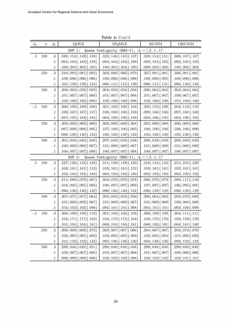
Table 4: Cont’d



.5 100 .3 .338(.154)[.149]{.139} .323(.146)[.145]{.137} .328(.154)[.151] .306(.167)[.167].1 .094(.163)[.163]{.159} .094(.163)[.163]{.169} .093(.162)[.162] .092(.165)[.165].1 .100(.204)[.204]{.195} .100(.204)[.204]{.195} .099(.202)[.202] .100(.202)[.202]

250 .3 .310(.082)[.081]{.082} .303(.080)[.080]{.079} .307(.081)[.081] .300(.081)[.081].1 .109(.096)[.096]{.096} .109(.096)[.096]{.096} .109(.096)[.095] .108(.096)[.096].1 .101(.139)[.139]{.134} .096(.141)[.141]{.139} .096(.141)[.141] .096(.140)[.140]

500 .3 .308(.060)[.059]{.059} .304(.059)[.058]{.056} .306(.064)[.064] .302(.064)[.064].1 .101(.067)[.067]{.068} .101(.067)[.067]{.068} .101(.067)[.067] .100(.067)[.067].1 .102(.100)[.100]{.098} .102(.100)[.100]{.098} .102(.100)[.100] .101(.100)[.100]

-.5 100 .3 .306(.109)[.109]{.106} .301(.108)[.108]{.104} .305(.110)[.109] .304(.110)[.110].1 .100(.167)[.167]{.157} .100(.168)[.168]{.159} .099(.166)[.166] .097(.168)[.168].1 .087(.195)[.194]{.185} .084(.199)[.198]{.189} .082(.196)[.195] .082(.196)[.195]

250 .3 .303(.069)[.069]{.069} .303(.069)[.069]{.068} .305(.069)[.069] .306(.069)[.069].1 .097(.099)[.098]{.095} .107(.100)[.100]{.095} .106(.100)[.100] .106(.100)[.099].1 .096(.138)[.138]{.134} .106(.138)[.138]{.133} .105(.138)[.138] .105(.138)[.138]

500 .3 .301(.048)[.048]{.048} .297(.049)[.049]{.048} .298(.049)[.049] .298(.049)[.049].1 .100(.069)[.069]{.067} .101(.069)[.069]{.067} .101(.069)[.069] .101(.069)[.069].1 .100(.097)[.097]{.098} .100(.097)[.097]{.098} .100(.097)[.097] .100(.097)[.097]


.5 100 .3 .327(.136)[.133]{.128} .311(.129)[.129]{.120} .318(.134)[.133] .251(.234)[.229].1 .103(.161)[.161]{.153} .103(.161)[.161]{.152} .103(.161)[.161] .102(.161)[.161].1 .103(.194)[.194]{.189} .094(.194)[.194]{.180} .092(.193)[.193] .093(.192)[.192]

250 .3 .311(.080)[.079]{.087} .304(.078)[.078]{.078} .308(.079)[.079] .280(.111)[.110].1 .104(.095)[.095]{.093} .108(.097)[.097]{.093} .107(.097)[.097] .106(.095)[.095].1 .096(.130)[.130]{.132} .096(.130)[.130]{.132} .096(.129)[.129] .096(.129)[.129]

500 .3 .307(.057)[.057]{.064} .305(.058)[.058]{.056} .306(.064)[.063] .292(.070)[.069].1 .101(.069)[.069]{.067} .101(.069)[.069]{.067} .101(.069)[.069] .100(.068)[.068].1 .104(.102)[.102]{.098} .094(.101)[.101]{.098} .094(.101)[.101] .092(.100)[.099]

-.5 100 .3 .306(.109)[.109]{.110} .301(.108)[.108]{.103} .306(.109)[.109] .304(.111)[.111].1 .104(.171)[.171]{.162} .104(.172)[.172]{.164} .103(.170)[.170] .103(.159)[.159].1 .101(.194)[.194]{.181} .089(.194)[.194]{.181} .088(.192)[.191] .084(.181)[.180]

250 .3 .300(.069)[.069]{.072} .302(.067)[.067]{.066} .304(.067)[.067] .303(.070)[.070].1 .103(.095)[.095]{.093} .103(.095)[.095]{.093} .102(.095)[.094] .101(.092)[.092].1 .101(.133)[.133]{.132} .095(.138)[.138]{.130} .094(.138)[.138] .093(.133)[.133]

500 .3 .299(.048)[.048]{.051} .298(.048)[.048]{.048} .299(.048)[.048] .299(.049)[.049].1 .102(.067)[.067]{.068} .102(.067)[.067]{.068} .101(.067)[.067] .100(.066)[.066].1 .099(.099)[.099]{.096} .103(.103)[.103]{.098} .103(.102)[.102] .103(.101)[.101]

36


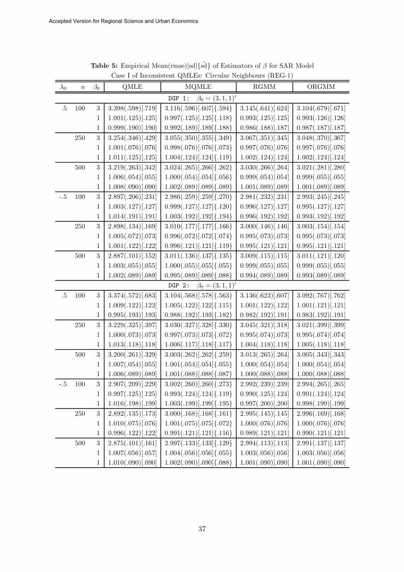
Table 5: Empirical Mean(rmse)[sd]{sd} of Estimators of β for SAR ModelCase I of Inconsistent QMLEs: Circular Neighbours (REG-1)


DGP 1: β0 = (3, 1, 1)′

.5 100 3 3.398(.598)[.719] 3.116(.596)[.607]{.594} 3.145(.641)[.624] 3.104(.679)[.671]1 1.001(.125)[.125] 0.997(.125)[.125]{.118} 0.993(.125)[.125] 0.993(.126)[.126]1 0.999(.190)[.190] 0.992(.189)[.189]{.188} 0.986(.188)[.187] 0.987(.187)[.187]

250 3 3.254(.346)[.429] 3.055(.350)[.355]{.349} 3.067(.351)[.345] 3.048(.370)[.367]1 1.001(.076)[.076] 0.998(.076)[.076]{.073} 0.997(.076)[.076] 0.997(.076)[.076]1 1.011(.125)[.125] 1.004(.124)[.124]{.119} 1.002(.124)[.124] 1.002(.124)[.124]

500 3 3.219(.263)[.342] 3.024(.265)[.266]{.262} 3.030(.266)[.264] 3.021(.281)[.280]1 1.006(.054)[.055] 1.000(.054)[.054]{.056} 0.999(.054)[.054] 0.999(.055)[.055]1 1.008(.090)[.090] 1.002(.089)[.089]{.089} 1.001(.089)[.089] 1.001(.089)[.089]

-.5 100 3 2.897(.206)[.231] 2.986(.259)[.259]{.270} 2.981(.232)[.231] 2.993(.245)[.245]1 1.003(.127)[.127] 0.999(.127)[.127]{.120} 0.996(.127)[.127] 0.995(.127)[.127]1 1.014(.191)[.191] 1.003(.192)[.192]{.194} 0.996(.192)[.192] 0.993(.192)[.192]

250 3 2.898(.134)[.169] 3.010(.177)[.177]{.166} 3.000(.146)[.146] 3.003(.154)[.154]1 1.005(.072)[.073] 0.996(.072)[.072]{.074} 0.995(.073)[.073] 0.995(.073)[.073]1 1.001(.122)[.122] 0.996(.121)[.121]{.119} 0.995(.121)[.121] 0.995(.121)[.121]

500 3 2.887(.101)[.152] 3.011(.136)[.137]{.135} 3.009(.115)[.115] 3.011(.121)[.120]1 1.003(.055)[.055] 1.000(.055)[.055]{.055} 0.999(.055)[.055] 0.999(.055)[.055]1 1.002(.089)[.089] 0.995(.089)[.089]{.088} 0.994(.089)[.089] 0.993(.089)[.089]

DGP 2: β0 = (3, 1, 1)′

.5 100 3 3.374(.572)[.683] 3.104(.568)[.578]{.563} 3.136(.623)[.607] 3.092(.767)[.762]1 1.009(.122)[.122] 1.005(.122)[.122]{.115} 1.001(.122)[.122] 1.001(.121)[.121]1 0.995(.193)[.193] 0.988(.192)[.193]{.182} 0.982(.192)[.191] 0.983(.192)[.191]

250 3 3.229(.325)[.397] 3.030(.327)[.328]{.330} 3.045(.321)[.318] 3.021(.399)[.399]1 1.000(.073)[.073] 0.997(.073)[.073]{.072} 0.995(.074)[.073] 0.995(.074)[.074]1 1.013(.118)[.118] 1.006(.117)[.118]{.117} 1.004(.118)[.118] 1.005(.118)[.118]

500 3 3.200(.261)[.329] 3.003(.262)[.262]{.259} 3.013(.265)[.264] 3.005(.343)[.343]1 1.007(.054)[.055] 1.001(.054)[.054]{.055} 1.000(.054)[.054] 1.000(.054)[.054]1 1.006(.089)[.089] 1.001(.088)[.088]{.087} 1.000(.088)[.088] 1.000(.088)[.088]

-.5 100 3 2.907(.209)[.229] 3.002(.260)[.260]{.273} 2.992(.239)[.239] 2.994(.265)[.265]1 0.997(.125)[.125] 0.993(.124)[.124]{.119} 0.990(.125)[.124] 0.991(.124)[.124]1 1.016(.198)[.199] 1.003(.199)[.199]{.195} 0.997(.200)[.200] 0.998(.199)[.199]

250 3 2.892(.135)[.173] 3.000(.168)[.168]{.161} 2.995(.145)[.145] 2.996(.169)[.168]1 1.010(.075)[.076] 1.001(.075)[.075]{.072} 1.000(.076)[.076] 1.000(.076)[.076]1 0.996(.122)[.122] 0.991(.121)[.121]{.116} 0.989(.121)[.121] 0.990(.121)[.121]

500 3 2.875(.101)[.161] 2.997(.133)[.133]{.129} 2.994(.113)[.113] 2.991(.137)[.137]1 1.007(.056)[.057] 1.004(.056)[.056]{.055} 1.003(.056)[.056] 1.003(.056)[.056]1 1.010(.090)[.090] 1.002(.090)[.090]{.088} 1.001(.090)[.090] 1.001(.090)[.090]

37


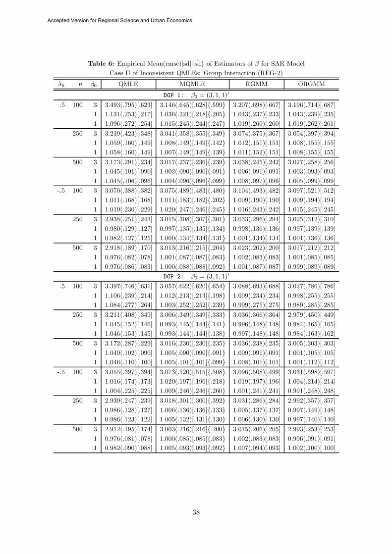
Table 6: Empirical Mean(rmse)[sd]{sd} of Estimators of β for SAR ModelCase II of Inconsistent QMLEs: Group Interaction (REG-2)


DGP 1: β0 = (3, 1, 1)′

.5 100 3 3.493(.795)[.623] 3.146(.645)[.628]{.599} 3.207(.698)[.667] 3.196(.714)[.687]1 1.131(.253)[.217] 1.036(.221)[.218]{.205} 1.043(.237)[.233] 1.043(.239)[.235]1 1.096(.272)[.254] 1.015(.245)[.244]{.247} 1.019(.260)[.260] 1.019(.262)[.261]

250 3 3.239(.423)[.348] 3.041(.358)[.355]{.349} 3.074(.375)[.367] 3.054(.397)[.394]1 1.059(.160)[.149] 1.008(.149)[.149]{.142} 1.012(.151)[.151] 1.008(.155)[.155]1 1.058(.160)[.149] 1.007(.149)[.149]{.139} 1.011(.152)[.151] 1.008(.155)[.155]

500 3 3.173(.291)[.234] 3.017(.237)[.236]{.239} 3.038(.245)[.242] 3.027(.258)[.256]1 1.045(.101)[.090] 1.002(.090)[.090]{.091} 1.006(.091)[.091] 1.003(.093)[.093]1 1.045(.106)[.096] 1.004(.096)[.096]{.099} 1.008(.097)[.096] 1.005(.099)[.099]

-.5 100 3 3.070(.388)[.382] 3.075(.489)[.483]{.480} 3.104(.493)[.482] 3.097(.521)[.512]1 1.011(.168)[.168] 1.011(.183)[.182]{.202} 1.009(.190)[.190] 1.009(.194)[.194]1 1.019(.230)[.229] 1.020(.247)[.246]{.245} 1.016(.243)[.242] 1.015(.245)[.245]

250 3 2.938(.251)[.243] 3.015(.308)[.307]{.301} 3.033(.296)[.294] 3.025(.312)[.310]1 0.980(.129)[.127] 0.997(.135)[.135]{.134} 0.998(.136)[.136] 0.997(.139)[.139]1 0.982(.127)[.125] 1.000(.134)[.134]{.131} 1.001(.134)[.134] 1.001(.136)[.136]

500 3 2.918(.189)[.170] 3.013(.216)[.215]{.204} 3.023(.202)[.200] 3.017(.212)[.212]1 0.976(.082)[.078] 1.001(.087)[.087]{.083} 1.002(.083)[.083] 1.001(.085)[.085]1 0.976(.086)[.083] 1.000(.088)[.088]{.092} 1.001(.087)[.087] 0.999(.089)[.089]

DGP 2: β0 = (3, 1, 1)′

.5 100 3 3.397(.746)[.631] 3.057(.622)[.620]{.654} 3.088(.693)[.688] 3.027(.786)[.786]1 1.106(.239)[.214] 1.012(.213)[.213]{.198} 1.009(.234)[.234] 0.998(.255)[.255]1 1.084(.277)[.264] 1.003(.252)[.252]{.239} 0.999(.275)[.275] 0.989(.285)[.285]

250 3 3.211(.408)[.349] 3.006(.349)[.349]{.333} 3.036(.366)[.364] 2.979(.450)[.449]1 1.045(.152)[.146] 0.993(.145)[.144]{.141} 0.996(.148)[.148] 0.984(.165)[.165]1 1.046(.153)[.145] 0.993(.144)[.144]{.138} 0.997(.148)[.148] 0.984(.163)[.162]

500 3 3.172(.287)[.229] 3.016(.230)[.230]{.235} 3.036(.238)[.235] 3.005(.303)[.303]1 1.049(.102)[.090] 1.005(.090)[.090]{.091} 1.009(.091)[.091] 1.001(.105)[.105]1 1.046(.110)[.100] 1.005(.101)[.101]{.099} 1.008(.101)[.101] 1.001(.112)[.112]

-.5 100 3 3.055(.397)[.394] 3.073(.520)[.515]{.508} 3.096(.508)[.499] 3.031(.598)[.597]1 1.016(.174)[.173] 1.020(.197)[.196]{.218} 1.019(.197)[.196] 1.004(.214)[.214]1 1.004(.225)[.225] 1.009(.246)[.246]{.260} 1.001(.241)[.241] 0.991(.248)[.248]

250 3 2.939(.247)[.239] 3.018(.301)[.300]{.392} 3.031(.286)[.284] 2.992(.357)[.357]1 0.986(.128)[.127] 1.006(.136)[.136]{.133} 1.005(.137)[.137] 0.997(.149)[.148]1 0.986(.123)[.122] 1.005(.132)[.131]{.130} 1.006(.130)[.130] 0.997(.140)[.140]

500 3 2.912(.195)[.174] 3.003(.216)[.216]{.200} 3.015(.206)[.205] 2.993(.253)[.253]1 0.976(.081)[.078] 1.000(.085)[.085]{.083} 1.002(.083)[.083] 0.996(.091)[.091]1 0.982(.090)[.088] 1.005(.093)[.093]{.092} 1.007(.094)[.093] 1.002(.100)[.100]

38


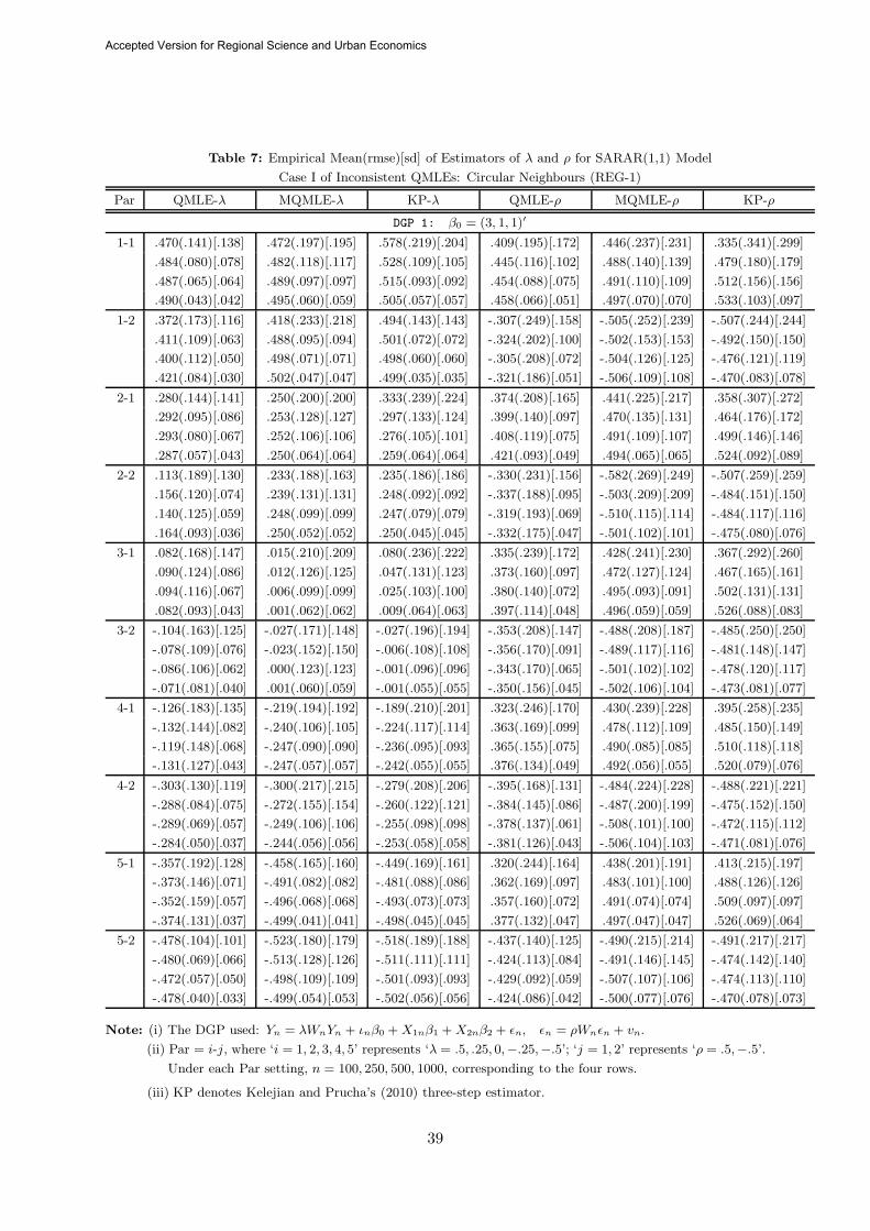
Table 7: Empirical Mean(rmse)[sd] of Estimators of λ and ρ for SARAR(1,1) Model

Case I of Inconsistent QMLEs: Circular Neighbours (REG-1)

Par QMLE-λ MQMLE-λ KP-λ QMLE-ρ MQMLE-ρ KP-ρ

DGP 1: β0 = (3, 1, 1)′

1-1 .470(.141)[.138] .472(.197)[.195] .578(.219)[.204] .409(.195)[.172] .446(.237)[.231] .335(.341)[.299]

.484(.080)[.078] .482(.118)[.117] .528(.109)[.105] .445(.116)[.102] .488(.140)[.139] .479(.180)[.179]

.487(.065)[.064] .489(.097)[.097] .515(.093)[.092] .454(.088)[.075] .491(.110)[.109] .512(.156)[.156]

.490(.043)[.042] .495(.060)[.059] .505(.057)[.057] .458(.066)[.051] .497(.070)[.070] .533(.103)[.097]

1-2 .372(.173)[.116] .418(.233)[.218] .494(.143)[.143] -.307(.249)[.158] -.505(.252)[.239] -.507(.244)[.244]

.411(.109)[.063] .488(.095)[.094] .501(.072)[.072] -.324(.202)[.100] -.502(.153)[.153] -.492(.150)[.150]

.400(.112)[.050] .498(.071)[.071] .498(.060)[.060] -.305(.208)[.072] -.504(.126)[.125] -.476(.121)[.119]

.421(.084)[.030] .502(.047)[.047] .499(.035)[.035] -.321(.186)[.051] -.506(.109)[.108] -.470(.083)[.078]

2-1 .280(.144)[.141] .250(.200)[.200] .333(.239)[.224] .374(.208)[.165] .441(.225)[.217] .358(.307)[.272]

.292(.095)[.086] .253(.128)[.127] .297(.133)[.124] .399(.140)[.097] .470(.135)[.131] .464(.176)[.172]

.293(.080)[.067] .252(.106)[.106] .276(.105)[.101] .408(.119)[.075] .491(.109)[.107] .499(.146)[.146]

.287(.057)[.043] .250(.064)[.064] .259(.064)[.064] .421(.093)[.049] .494(.065)[.065] .524(.092)[.089]

2-2 .113(.189)[.130] .233(.188)[.163] .235(.186)[.186] -.330(.231)[.156] -.582(.269)[.249] -.507(.259)[.259]

.156(.120)[.074] .239(.131)[.131] .248(.092)[.092] -.337(.188)[.095] -.503(.209)[.209] -.484(.151)[.150]

.140(.125)[.059] .248(.099)[.099] .247(.079)[.079] -.319(.193)[.069] -.510(.115)[.114] -.484(.117)[.116]

.164(.093)[.036] .250(.052)[.052] .250(.045)[.045] -.332(.175)[.047] -.501(.102)[.101] -.475(.080)[.076]

3-1 .082(.168)[.147] .015(.210)[.209] .080(.236)[.222] .335(.239)[.172] .428(.241)[.230] .367(.292)[.260]

.090(.124)[.086] .012(.126)[.125] .047(.131)[.123] .373(.160)[.097] .472(.127)[.124] .467(.165)[.161]

.094(.116)[.067] .006(.099)[.099] .025(.103)[.100] .380(.140)[.072] .495(.093)[.091] .502(.131)[.131]

.082(.093)[.043] .001(.062)[.062] .009(.064)[.063] .397(.114)[.048] .496(.059)[.059] .526(.088)[.083]

3-2 -.104(.163)[.125] -.027(.171)[.148] -.027(.196)[.194] -.353(.208)[.147] -.488(.208)[.187] -.485(.250)[.250]

-.078(.109)[.076] -.023(.152)[.150] -.006(.108)[.108] -.356(.170)[.091] -.489(.117)[.116] -.481(.148)[.147]

-.086(.106)[.062] .000(.123)[.123] -.001(.096)[.096] -.343(.170)[.065] -.501(.102)[.102] -.478(.120)[.117]

-.071(.081)[.040] .001(.060)[.059] -.001(.055)[.055] -.350(.156)[.045] -.502(.106)[.104] -.473(.081)[.077]

4-1 -.126(.183)[.135] -.219(.194)[.192] -.189(.210)[.201] .323(.246)[.170] .430(.239)[.228] .395(.258)[.235]

-.132(.144)[.082] -.240(.106)[.105] -.224(.117)[.114] .363(.169)[.099] .478(.112)[.109] .485(.150)[.149]

-.119(.148)[.068] -.247(.090)[.090] -.236(.095)[.093] .365(.155)[.075] .490(.085)[.085] .510(.118)[.118]

-.131(.127)[.043] -.247(.057)[.057] -.242(.055)[.055] .376(.134)[.049] .492(.056)[.055] .520(.079)[.076]

4-2 -.303(.130)[.119] -.300(.217)[.215] -.279(.208)[.206] -.395(.168)[.131] -.484(.224)[.228] -.488(.221)[.221]

-.288(.084)[.075] -.272(.155)[.154] -.260(.122)[.121] -.384(.145)[.086] -.487(.200)[.199] -.475(.152)[.150]

-.289(.069)[.057] -.249(.106)[.106] -.255(.098)[.098] -.378(.137)[.061] -.508(.101)[.100] -.472(.115)[.112]

-.284(.050)[.037] -.244(.056)[.056] -.253(.058)[.058] -.381(.126)[.043] -.506(.104)[.103] -.471(.081)[.076]

5-1 -.357(.192)[.128] -.458(.165)[.160] -.449(.169)[.161] .320(.244)[.164] .438(.201)[.191] .413(.215)[.197]

-.373(.146)[.071] -.491(.082)[.082] -.481(.088)[.086] .362(.169)[.097] .483(.101)[.100] .488(.126)[.126]

-.352(.159)[.057] -.496(.068)[.068] -.493(.073)[.073] .357(.160)[.072] .491(.074)[.074] .509(.097)[.097]

-.374(.131)[.037] -.499(.041)[.041] -.498(.045)[.045] .377(.132)[.047] .497(.047)[.047] .526(.069)[.064]

5-2 -.478(.104)[.101] -.523(.180)[.179] -.518(.189)[.188] -.437(.140)[.125] -.490(.215)[.214] -.491(.217)[.217]

-.480(.069)[.066] -.513(.128)[.126] -.511(.111)[.111] -.424(.113)[.084] -.491(.146)[.145] -.474(.142)[.140]

-.472(.057)[.050] -.498(.109)[.109] -.501(.093)[.093] -.429(.092)[.059] -.507(.107)[.106] -.474(.113)[.110]

-.478(.040)[.033] -.499(.054)[.053] -.502(.056)[.056] -.424(.086)[.042] -.500(.077)[.076] -.470(.078)[.073]

Note: (i) The DGP used: Yn = λWnYn + ιnβ0 + X1nβ1 + X2nβ2 + εn, εn = ρWnεn + vn.

(ii) Par = i-j, where ‘i = 1, 2, 3, 4, 5’ represents ‘λ = .5, .25, 0,−.25,−.5’; ‘j = 1, 2’ represents ‘ρ = .5,−.5’.

Under each Par setting, n = 100, 250, 500, 1000, corresponding to the four rows.

(iii) KP denotes Kelejian and Prucha’s (2010) three-step estimator.

39


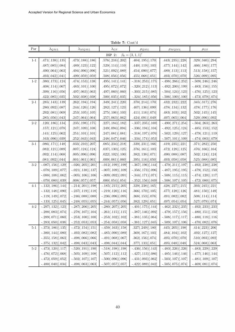
Table 7: Cont’d

Par λQML λMQML λGS ρQML ρMQML ρGS

DGP 2: β0 = (3, 1, 1)′

1-1 .471(.138)[.135] .473(.188)[.186] .576(.216)[.202] .404(.195)[.170] .443(.235)[.228] .329(.340)[.294]

.487(.085)[.084] .489(.123)[.122] .529(.114)[.110] .440(.119)[.103] .477(.144)[.142] .466(.180)[.177]

.490(.064)[.063] .494(.096)[.096] .521(.092)[.089] .454(.090)[.077] .489(.113)[.113] .513(.158)[.157]

.493(.042)[.041] .499(.059)[.059] .508(.056)[.056] .455(.068)[.051] .493(.070)[.070] .526(.099)[.095]

1-2 .380(.173)[.124] .474(.153)[.138] .495(.141)[.141] -.318(.253)[.175] -.498(.266)[.252] -.509(.246)[.246]

.408(.114)[.067] .483(.101)[.100] .495(.072)[.072] -.320(.212)[.113] -.492(.200)[.199] -.483(.156)[.155]

.399(.116)[.056] .497(.063)[.063] .497(.060)[.060] -.303(.215)[.085] -.504(.124)[.123] -.476(.125)[.123]

.422(.085)[.035] .502(.038)[.038] .500(.035)[.035] -.324(.185)[.056] -.506(.100)[.100] -.473(.079)[.074]

2-1 .285(.143)[.139] .262(.194)[.194] .349(.241)[.220] .370(.214)[.170] .432(.232)[.222] .345(.317)[.276]

.280(.092)[.087] .244(.126)[.126] .282(.127)[.123] .407(.136)[.099] .478(.134)[.132] .478(.177)[.176]

.292(.081)[.069] .253(.105)[.105] .275(.106)[.103] .411(.116)[.074] .483(.103)[.102] .502(.145)[.145]

.285(.056)[.043] .247(.064)[.064] .257(.063)[.062] .424(.091)[.049] .497(.065)[.064] .529(.096)[.092]

2-2 .120(.186)[.134] .235(.198)[.175] .227(.184)[.182] -.337(.235)[.169] -.490(.271)[.254] -.504(.263)[.263]

.157(.121)[.078] .247(.109)[.108] .249(.094)[.094] -.336(.194)[.104] -.492(.125)[.124] -.485(.153)[.152]

.141(.125)[.062] .251(.101)[.101] .247(.081)[.081] -.318(.197)[.076] -.502(.129)[.127] -.479(.121)[.119]

.163(.096)[.039] .252(.043)[.043] .248(.047)[.046] -.334(.174)[.053] -.507(.101)[.109] -.474(.083)[.079]

3-1 .086(.171)[.148] .033(.210)[.207] .085(.234)[.218] .339(.231)[.166] .419(.235)[.221] .371(.282)[.250]

.082(.121)[.089] .007(.124)[.124] .037(.130)[.125] .376(.161)[.103] .472(.128)[.125] .476(.166)[.164]

.092(.114)[.068] .005(.096)[.096] .022(.102)[.100] .382(.138)[.071] .490(.088)[.087] .502(.124)[.124]

.081(.092)[.044] .001(.061)[.061] .009(.061)[.060] .395(.116)[.050] .493(.058)[.058] .525(.088)[.085]

3-2 -.087(.156)[.129] -.026(.205)[.201] -.012(.199)[.199] -.367(.196)[.144] -.479(.211)[.197] -.492(.238)[.238]

-.078(.109)[.077] -.021(.138)[.137] -.007(.109)[.109] -.356(.173)[.096] -.487(.195)[.195] -.479(.152)[.150]

-.088(.108)[.062] -.005(.106)[.106] -.009(.092)[.091] -.344(.171)[.071] -.508(.115)[.115] -.474(.120)[.117]

-.070(.080)[.039] .008(.057)[.057] .000(.054)[.054] -.352(.156)[.049] -.508(.107)[.105] -.472(.080)[.075]

4-1 -.132(.186)[.144] -.214(.201)[.198] -.185(.215)[.205] .329(.238)[.165] .428(.227)[.215] .393(.245)[.221]

-.132(.148)[.090] -.237(.119)[.118] -.219(.120)[.116] .366(.170)[.105] .477(.128)[.126] .481(.150)[.149]

-.119(.149)[.072] -.246(.088)[.088] -.236(.096)[.095] .368(.153)[.076] .491(.082)[.082] .508(.114)[.114]

-.133(.125)[.045] -.248(.055)[.055] -.244(.057)[.056] .382(.129)[.051] .497(.054)[.054] .527(.079)[.074]

4-2 -.297(.132)[.123] -.287(.206)[.205] -.280(.207)[.205] -.401(.175)[.144] -.462(.232)[.235] -.492(.233)[.233]

-.288(.083)[.074] -.278(.107)[.104] -.261(.115)[.115] -.387(.146)[.092] -.479(.157)[.156] -.480(.151)[.150]

-.289(.071)[.060] -.253(.100)[.100] -.253(.102)[.102] -.381(.135)[.064] -.508(.117)[.117] -.480(.118)[.116]

-.283(.050)[.038] -.252(.053)[.053] -.254(.058)[.058] -.381(.127)[.045] -.509(.107)[.106] -.470(.082)[.076]

5-1 -.373(.186)[.135] -.472(.154)[.151] -.459(.163)[.158] .327(.249)[.180] .445(.205)[.198] .414(.223)[.206]

-.380(.144)[.080] -.492(.082)[.082] -.485(.090)[.089] .369(.167)[.103] .484(.104)[.102] .492(.127)[.127]

-.355(.158)[.063] -.498(.066)[.066] -.491(.068)[.067] .362(.156)[.074] .495(.070)[.070] .510(.093)[.092]

-.375(.132)[.042] -.498(.043)[.043] -.498(.044)[.044] .377(.133)[.051] .495(.048)[.048] .524(.068)[.063]

5-2 -.473(.120)[.117] -.520(.191)[.190] -.518(.198)[.198] -.436(.156)[.143] -.483(.226)[.226] -.483(.229)[.229]

-.476(.072)[.068] -.505(.109)[.108] -.507(.112)[.112] -.427(.113)[.086] -.485(.146)[.146] -.477(.146)[.144]

-.472(.059)[.052] -.502(.107)[.107] -.500(.096)[.096] -.431(.093)[.062] -.503(.107)[.107] -.481(.109)[.107]

-.480(.040)[.034] -.498(.063)[.063] -.507(.057)[.057] -.422(.089)[.042] -.505(.075)[.074] -.469(.081)[.074]

40


Modiﬁed QML Estimation of Spatial Autoregressive … Publications...While heteroskedasticity is...

Documents

Transcript of Modiﬁed QML Estimation of Spatial Autoregressive … Publications...While heteroskedasticity is...