Modi cations of Q-learning to Optimize Dynamic Treatment ...

Modifications of Q-learning to OptimizeDynamic Treatment Regimes

A DISSERTATION

SUBMITTED TO THE FACULTY OF THE GRADUATE SCHOOL

OF THE UNIVERSITY OF MINNESOTA

BY

Yuan Zhang

IN PARTIAL FULFILLMENT OF THE REQUIREMENTS

FOR THE DEGREE OF

DOCTOR OF PHILOSOPHY

Advised by Thomas A. Murray, Ph.D.

Co-advised by David M. Vock, Ph.D.

August, 2021

Acknowledgements

First and foremost it is a genuine pleasure to express my sincere gratitude to my ad-

visers Dr. Tom Murray and Dr. David Vock for their invaluable advice, support, and

encouragement during my PhD study. I am extremely fortunate to work with Tom who

always has great ideas and provides continuous guidance and patience throughout my

research. I have also received ingenious suggestions from David not only for the comple-

tion of this dissertation, but also on the insights into academia, methodological research

and interdisciplinary collaboration as a whole. Many thanks to Dr. Megan Patrick for

providing the M-bridge data to illustrate our proposed methods, and Grace Lyden for

her generous assistance in processing the raw data. I would also like to acknowledge

Dr. Lizbeth Finestack for serving on my committee and initiating the first project of

the thesis.

I am deeply grateful to Dr. Lynn Eberly for her mentorship on my work as a re-

search assistant in the diabetes projects. Lynn, together with the principal investigators

Dr. Elizabeth Seaquist and Dr. Gulin Oz, serving as excellent role models for female

researchers, has inspired and motivated me in the pursuit of an academic career. It is

indeed my privilege to spend more than three years in the Seaquist Lab and collaborate

with the wonderful team. I have received tremendous help from Evan Olawsky, Anjali

Kumar, Michelle Snyder, Dr. Amir Moheet and Dr. Lisa Chow. I would also like to

extend my appreciation to Dr. Silvia Mangia and Dr. Antonietta Canna for their trust

and compliment on my independent analyses of neuroimaging data.

i

Furthermore, I wish to offer my special thanks to my internship mentor at the Merck

Research Laboratories, Dr. John Kang, who has expanded my horizons by exemplifying

biometrics research in drug development. I vastly enjoyed the respectful and innovative

working environment and the interesting project of adjusting for treatment switching in

oncology studies. It was really a great step forward and contributed to my confidence

in developing statistical methods within a time constraint.

I am indebted to the Division of Biostatistics, the University of Minnesota. I very

much appreciate the extensive help from Sally Olander since the very first day I arrived

at the division. Thanks should also go to Susan Wei for giving the most intellectually

engaging lectures and providing me with useful tips to survive through the winter in

Minnesota. My journey as a PhD student would not be complete without friends who

never wavered in their support. I must thank Chuyu Deng and Shannon McKearnan

for their kindness since I joined the cohort, Mengli Xiao and Tianzhong Yang for their

company during the pandemic, and Jin Jin for talking me through everything.

Finally, I gratefully thank my dearest parents for always believing in me and re-

specting every decision I have ever made, and my fiance for always taking great care of

me. Without their trust and support I could not have made it this far. I would also like

to thank my lifelong best friends Yilin Qiao, Shengyun Wang and Wenxin Tian who

live in different continents but always understand and support me one way or another.

ii

This dissertation is dedicated to my fiance Tingyang Zhou

and my parents Wei Su and Jianfeng Zhang

for their endless love, trust and support.

iii

Abstract

With an emerging interest in personalized medicine and quality healthcare, the design

of clinical trials that incorporates multiple stages of randomization and intervention, for

example, a sequential multiple assignment randomized trial (SMART), has become a

popular choice for investigators as it facilitates the construction and analysis of dynamic

treatment regimes (DTRs). There exists a comprehensive body of literature on various

statistical methods to analyze data collected from such trials and estimate the optimal

DTR for an individual subject, among which Q-learning with linear regression is widely

used due to its simplicity and ease of interpretation. This thesis discusses three impor-

tant challenges that cause problems in the implementation of Q-learning and proposes

multiple modifications of Q-learning to address them.

The first challenge arises from the repeatedly monitored outcome of interest at in-

termediate stages of randomization and at longer follow-up intervals after the final stage

of randomization. Clinical investigators are usually interested in identifying the optimal

DTR and estimating the outcome trajectory under the optimal DTR. However, in the

presence of stagewise repeated-measures outcomes, standard Q-learning fails to provide

point estimates of the optimal trajectory with time-specific heterogeneous causal effects.

To address this problem, we propose a modified algorithm of Q-learning with a gener-

alized estimating equation to estimate each Q-function. The second challenge is model

misspecification. Model misspecification is a common problem in Q-learning, but little

attention has been given to its impact when treatment effects are heterogeneous across

subjects. We describe the integrative impact of two possible types of model misspecifica-

tion related to treatment effect heterogeneity: unexplained early-stage treatment effects

in late-stage main effect model, and misspecified linearity between pseudo-outcomes and

predictors as a result of the optimization operation. The proposed method, aiming to

deal with both types of misspecification concomitantly, builds interactive models into

iv

residual-modified parametric Q-learning. The third challenge is generalizing modified

Q-learning to dichotomous outcomes. It is difficult to include informative residuals from

estimation of late-stage models into early-stage pseudo-outcomes due to the non-identity

link function. We propose a modification based on monotonicity of preferences to ad-

dress model misspecification in Q-learning with probit regression. The improvement

in robustness of the proposed modification is subject to the extent of model misspec-

ification and can be limited. Thus, we take a latent variable approach and propose a

novel algorithm using sampled surrogates of the underlying continuous outcome condi-

tional on the binary observations. The methods proposed in this thesis are assessed via

simulations and illustrated using the M-bridge study, a SMART with embedded tailor-

ing which develops and evaluates adaptive interventions for preventing binge drinking

among college students.

v

Contents

Acknowledgements i

Abstract iv

List of Tables x

List of Figures xii

1 Introduction 1

1.1 Overview . . . . . . . . . . . . . . . . . . . . . . . . . . . . . . . . . . . 1

1.2 Q-learning: A Backward Induction Algorithm . . . . . . . . . . . . . . . 2

1.3 The M-bridge Study . . . . . . . . . . . . . . . . . . . . . . . . . . . . . 4

1.4 Outline . . . . . . . . . . . . . . . . . . . . . . . . . . . . . . . . . . . . 5

2 Modified Q-learning with Generalized Estimating Equations for Repeated-

measures Outcomes 7

2.1 Motivation . . . . . . . . . . . . . . . . . . . . . . . . . . . . . . . . . . 7

2.2 Statistical Framework for a SMART with Repeated-measures Outcomes 10

2.2.1 Causal Framework . . . . . . . . . . . . . . . . . . . . . . . . . . 10

2.2.2 Optimization Problem . . . . . . . . . . . . . . . . . . . . . . . . 12

2.3 Modified Q-learning with Generalized Estimating Equations . . . . . . . 13

2.3.1 Composite Q-learning . . . . . . . . . . . . . . . . . . . . . . . . 14

vi

2.3.2 Q-learning with Generalized Estimating Equations . . . . . . . . 14

2.3.3 Modified Q-learning with Murphy’s Regret Function . . . . . . . 17

2.4 Simulation Study . . . . . . . . . . . . . . . . . . . . . . . . . . . . . . . 18

2.4.1 Data Generative Mechanism . . . . . . . . . . . . . . . . . . . . 19

2.4.2 Evaluation Criteria . . . . . . . . . . . . . . . . . . . . . . . . . . 20

2.4.3 Results for Equally Weighted Outcomes . . . . . . . . . . . . . . 21

2.4.4 Results for Unequally Weighted Outcomes . . . . . . . . . . . . . 27

2.5 Application . . . . . . . . . . . . . . . . . . . . . . . . . . . . . . . . . . 28

2.5.1 Identification of Personalized Optimal Rules . . . . . . . . . . . . 29

2.5.2 Point Estimation of the Optimal Trajectory and Heterogeneous

Causal Effects . . . . . . . . . . . . . . . . . . . . . . . . . . . . . 30

2.6 Discussion . . . . . . . . . . . . . . . . . . . . . . . . . . . . . . . . . . . 32

3 On the Model Misspecification in Q-learning with Treatment Effect

Heterogeneity 33

3.1 Literature Review . . . . . . . . . . . . . . . . . . . . . . . . . . . . . . 33

3.2 Framework . . . . . . . . . . . . . . . . . . . . . . . . . . . . . . . . . . 35

3.2.1 Data Example . . . . . . . . . . . . . . . . . . . . . . . . . . . . 35

3.2.2 Data Structure . . . . . . . . . . . . . . . . . . . . . . . . . . . . 37

3.2.3 Q-learning . . . . . . . . . . . . . . . . . . . . . . . . . . . . . . . 38

3.3 Unmeasured Variables . . . . . . . . . . . . . . . . . . . . . . . . . . . . 39

3.3.1 Misspecification of Stage 2 Main Effects . . . . . . . . . . . . . . 39

3.3.2 Estimation Bias . . . . . . . . . . . . . . . . . . . . . . . . . . . 39

3.3.3 A Special Case: Omission of Stage 1 Heterogeneous Treatment

Effects . . . . . . . . . . . . . . . . . . . . . . . . . . . . . . . . . 41

3.4 Model Misspecification with Treatment Effect Heterogeneity . . . . . . . 42

3.5 The Proposed Method . . . . . . . . . . . . . . . . . . . . . . . . . . . . 45

3.5.1 Modified Interactive Q-learning . . . . . . . . . . . . . . . . . . . 45

vii

3.5.2 Small Sample Properties of the Proposed Estimator . . . . . . . 47

3.6 Simulation . . . . . . . . . . . . . . . . . . . . . . . . . . . . . . . . . . . 48

3.6.1 Preliminaries . . . . . . . . . . . . . . . . . . . . . . . . . . . . . 48

3.6.2 Results . . . . . . . . . . . . . . . . . . . . . . . . . . . . . . . . 50

3.7 Data Analysis . . . . . . . . . . . . . . . . . . . . . . . . . . . . . . . . . 52

3.8 Discussion . . . . . . . . . . . . . . . . . . . . . . . . . . . . . . . . . . . 56

4 A Generalization to Dichotomous Outcomes 57

4.1 Background . . . . . . . . . . . . . . . . . . . . . . . . . . . . . . . . . . 57

4.2 Methods . . . . . . . . . . . . . . . . . . . . . . . . . . . . . . . . . . . . 58

4.2.1 Q-learning with Probit Regression . . . . . . . . . . . . . . . . . 59

4.2.2 The Proposed Modification . . . . . . . . . . . . . . . . . . . . . 60

4.3 Simulation Study . . . . . . . . . . . . . . . . . . . . . . . . . . . . . . . 62

4.4 Data Analysis . . . . . . . . . . . . . . . . . . . . . . . . . . . . . . . . . 65

4.5 A Latent Variable Approach . . . . . . . . . . . . . . . . . . . . . . . . . 67

4.5.1 Framework . . . . . . . . . . . . . . . . . . . . . . . . . . . . . . 67

4.5.2 The Proposed Algorithm . . . . . . . . . . . . . . . . . . . . . . 68

4.5.3 Simulation Study Revisited . . . . . . . . . . . . . . . . . . . . . 70

4.5.4 Challenges with the Monotonicity Assumption . . . . . . . . . . 72

4.6 Discussion . . . . . . . . . . . . . . . . . . . . . . . . . . . . . . . . . . . 73

5 Conclusion 74

5.1 Summary . . . . . . . . . . . . . . . . . . . . . . . . . . . . . . . . . . . 74

5.2 Future Work . . . . . . . . . . . . . . . . . . . . . . . . . . . . . . . . . 75

Bibliography 77

Appendix A. Supplementary Materials for mQ-GEE 83

A.1 Inference for mQ-GEE . . . . . . . . . . . . . . . . . . . . . . . . . . . . 83

A.2 The DLD Study . . . . . . . . . . . . . . . . . . . . . . . . . . . . . . . 84

viii

A.3 Marginalization over an Unmeasured Covariate . . . . . . . . . . . . . . 85

A.4 Model Misspecifications in the Simulation Study . . . . . . . . . . . . . 87

A.5 Relative Efficiency Using Different Working Correlations . . . . . . . . . 88

A.6 Simulation Study: Parsimonious Models . . . . . . . . . . . . . . . . . . 89

A.7 Application: Model Fit and Variable Selection . . . . . . . . . . . . . . . 91

Appendix B. Supplementary Materials for mIQ 94

B.1 Proof . . . . . . . . . . . . . . . . . . . . . . . . . . . . . . . . . . . . . . 94

B.2 Additional Results for Data Analysis . . . . . . . . . . . . . . . . . . . . 100

Appendix C. Supplementary Materials for mLQ 101

C.1 The Manifest Distribution . . . . . . . . . . . . . . . . . . . . . . . . . . 101

C.2 Conditional Moments of the Latent Variable . . . . . . . . . . . . . . . . 102

ix

List of Tables

2.1 Simulation results for mQ-GEE with no model misspecification . . . . . 22

2.2 Simulation results for mQ-GEE with stage 2 main effect model misspec-

ification . . . . . . . . . . . . . . . . . . . . . . . . . . . . . . . . . . . . 23

2.3 Summary of estimated optimal rules under different weights as a propor-

tion of college students who were eligible for randomization . . . . . . . 29

3.1 Specification of the data generative mechanism . . . . . . . . . . . . . . 49

3.2 Percentage of correctly identified stage 1 optimal rules when stage 2 treat-

ment effects are homogeneous across subjects, using standard Q-learning

and interactive Q-learning . . . . . . . . . . . . . . . . . . . . . . . . . . 50

3.3 Percentage of correctly identified stage 1 optimal rules when stage 2

treatment effects are heterogeneous across subjects, using standard Q-

learning, modified Q-learning, interactive Q-learning, and modified in-

teractive Q-learning . . . . . . . . . . . . . . . . . . . . . . . . . . . . . 50

3.4 Summary statistics of subject characteristics in the M-bridge study . . . 52

3.5 Summary statistics of continuous outcomes in the M-bridge study . . . 54

4.1 Percentage of correctly identified optimal rules using Q-learning with

probit regression and modified Q-learning with probit regression . . . . 63

4.2 Summary statistics of dichotomous outcomes in the M-bridge study . . 65

4.3 Full data analysis results using Q-probit and mQ-probit . . . . . . . . . 66

x

A.1 Relative efficiency under different correlation structures based on a sam-

ple size of n = 200 and 1000 simulations . . . . . . . . . . . . . . . . . . 89

A.2 Simulation results for mQ-GEE with parsimonious models (no model

misspecification) . . . . . . . . . . . . . . . . . . . . . . . . . . . . . . . 90

A.3 Simulation results for mQ-GEE with parsimonious models (stage 2 main

effect model misspecification) . . . . . . . . . . . . . . . . . . . . . . . . 91

A.4 Summary of model fit and variable selection . . . . . . . . . . . . . . . . 91

B.1 Full data analysis results using sQ, mQ, IQ, and mIQ . . . . . . . . . . 100

xi

List of Figures

1.1 A sequential, multiple assignment, randomized trial of alcohol use dis-

order for first-year college students (the M-bridge study and the design

with repeated-measures outcomes) . . . . . . . . . . . . . . . . . . . . . 4

2.1 The probability of correctly identifying the optimal rules across a grid of

sample sizes based on 1000 iterations . . . . . . . . . . . . . . . . . . . . 24

2.2 Root mean square error of heterogeneous causal effects across a grid of

sample sizes based on 1000 iterations . . . . . . . . . . . . . . . . . . . . 25

2.3 Bias of heterogeneous causal effects across a grid of Z1 based on 1000

iterations . . . . . . . . . . . . . . . . . . . . . . . . . . . . . . . . . . . 26

2.4 The probability of correctly identifying the optimal rules across a set of

weights (w1,w2) based on 1000 iterations . . . . . . . . . . . . . . . . . 27

2.5 Root mean square error of heterogeneous causal effects across a set of

weights (w1,w2) based on 1000 iterations . . . . . . . . . . . . . . . . . 28

2.6 Estimated optimal trajectory versus marginal DTR-specific trajectories 30

2.7 Distribution of estimated heterogeneous causal effects using mQ-GEE . 31

3.1 A simple design of the M-bridge study with a final outcome at the end

of the treatment course . . . . . . . . . . . . . . . . . . . . . . . . . . . 36

3.2 Probability of correctly identifying stage 1 optimal rules as a function of

c2 for c1 = 0, 2, 4 . . . . . . . . . . . . . . . . . . . . . . . . . . . . . . . 51

xii

3.3 Residual diagnostics for (a) the parsimonious model (b) the saturated

model . . . . . . . . . . . . . . . . . . . . . . . . . . . . . . . . . . . . . 55


σ for different values of γ using Q-learning with probit regression . . . . 64


σ for different values of γ using modified latent Q-learning . . . . . . . . 71

A.1 A sequential, multiple assignment, randomized trial for children with

developmental language disorder (DLD) . . . . . . . . . . . . . . . . . . 84

xiii

Chapter 1

Introduction

1.1 Overview

With an increasing demand for quality healthcare and precision medicine, dynamic

treatment regime has become an emerging field for statistical researchers. A dynamic

treatment regime (DTR) (Murphy, 2003; Orellana et al., 2010; Chakraborty and Mur-

phy, 2014; Laber et al., 2014), also known as adaptive intervention (Collins et al., 2004;

Murphy et al., 2007; Lei et al., 2012; Nahum-Shani et al., 2020), or adaptive treatment

strategy (Lavori and Dawson, 2000; Murphy and McKay, 2004; Kosorok and Moodie,

2015), is a sequence of functions, one for each decision, which map from a participant’s

history of characteristics and actions to a set of possible subsequent actions to take over

time. The actions in general can be, depending on the context, treatments or inter-

ventions, and will be used interchangeably in this thesis. Such treatment regimes are

dynamic because individualized treatments vary according to tailoring variables (Collins

et al., 2004; Nahum-Shani et al., 2012). An example of a tailoring variable is whether a

participant responds to the treatment assigned at the first stage, and the correspond-

ing DTR might prescribe that responders continue the initial treatment at the second

stage, whereas non-responders switch to an alternative treatment. This adaptive and

1

2

sequential nature of treatment assignments take patient heterogeneity into account and

effectuates personalized medicine.

The sequential multiple assignment randomized trial (SMART) (Murphy, 2005a;

Lavori and Dawson, 2014; Collins et al., 2007) is an experimental design that allows

multiple stages of randomization and collects longitudinal data over these stages to help

construct and analyze DTRs. The two main goals of analyzing the data collected from

SMART studies are: (1) comparison between embedded DTRs, and (2) estimation of

the optimal DTR. The former approach aims to analyze deterministic dynamic regimes,

whereas the latter takes advantage of sequentially accrued information to individualize

treatment at subsequent stages so that the subject ends up with the best possible

result. This thesis focuses mainly on identifying the sequence of decision rules that

optimizes the outcome in question and estimating this value at each time point of

interest. Various methods to address this problem were proposed and discussed in

literature. Chakraborty and Murphy (2014) presented a comprehensive description of

direct and indirect methods to identify the optimal DTR, direct methods being marginal

structural models (Robins, 2000a,b) and inverse probability of treatment weighting, and

indirect methods including Q-learning and dynamic system models.

1.2 Q-learning: A Backward Induction Algorithm

Q-learning (Watkins, 1989) is a dynamic programming (Bellman, 1957) algorithm and

has been widely implemented to identify the optimal DTR (Murphy and McKay, 2004;

Nahum-Shani et al., 2012). At each stage of randomization, Q-learning specifies a model

of expected outcomes conditional on past history, given that the optimal interventions

are followed thereafter. The parametric form of the conditional expectation is called a

Q-function (Sutton and Barto, 1998; Murphy, 2005b) and is usually written as a linear

regression. Model parameters are estimated stagewise using backward induction (Au-

mann, 1995). In classification problems, the Q-functions may be estimated by regression

3

trees or kernels.

Suppose the longitudinal data collected from a SMART study are

(Z1, A1, Z2, A2, . . . , Zk, Ak, . . . , ZK , AK , Y )

for stages k = 1, . . . ,K, where Zk denotes the observed covariates and intermediate

outcomes which are measured prior to randomization at stage k, Ak ∈ Ak denotes the

treatment received at stage k, and Y denotes the final outcome of interest with small

values preferred. Let Hk = (Z1, A1, . . . , Zk−1, Ak−1, Zk) be the history of covariates and

treatments prior to randomization at stage k.

Optimization of DTRs borrows the concept of potential outcomes, and therefore the

following causal assumptions are necessary:

• Consistency: The potential outcome under the observed treatment agrees with

the observed outcome;

• No unmeasured confounders, also known as sequential ignorability: Ak is inde-

pendent of all future potential outcomes, conditional on the history Hk.

The no unmeasured confounders assumption is valid with the sequential randomization

of a SMART.

The Q-function at stage k, Qk(Hk, Ak), is a function of the observed history up to

stage k and the treatment received at stage k, and usually consists of a main effect

model and a treatment effect model.

Starting from the last stage, the linear regression model is specified as

QK(HK , AK) = E(Y |HK , AK) = xTK0βK +AKxTK1ψK ,

where xK0 and xK1 are realizations of functions of HK that represent the covariates in

the main effect and treatment effect model respectively. The least squares estimators

of stage K parameters, βK and ψK , are obtained.

4

For a precedent stage k, k = K − 1,K − 2, . . . , 1, the Q-function is specified as

Qk(Hk, Ak) = E[

minak+1∈Ak+1

Qk+1(Hk+1, Ak+1 = ak+1)

∣∣∣∣Hk, Ak

]= xTk0βk +Akx

Tk1ψk,

where xk0 and xk1 are realizations of functions of Hk. The least squares estimators of

stage k parameters, βk and ψk are obtained.

The estimated optimal DTR is(dopt

1 , . . . , doptk , . . . , dopt

K

), with

doptk = arg min

ak∈Ak

Qk(Hk, Ak = ak; βk, ψk).

We assume a two-stage setting throughout the thesis, where K = 2.

1.3 The M-bridge Study

Figure 1.1: The M-bridge study: a sequential, multiple assignment, randomized trial.

This figure is adapted from the figure of study design in Patrick et al. (2020). Rindicates a randomization stage with arrows pointing to available treatment options, and

A indicates time of assessment where measurements of intermediate or final outcometake place.

5

The M-bridge study (Patrick et al., 2020) is a SMART conducted at the Univer-

sity of Minnesota Twin Cities. The study develops and evaluates an adaptive pre-

ventive intervention for college drinking and related problems among first-year college

students. As illustrated in Figure 1.1, enrolled students were randomized to receiv-

ing a combined universal preventive intervention, personalized normative feedback and

self-monitoring (PNF+SM), either prior to attending college (early intervention) or in

the first month of the first semester (late intervention). Two intermediate measures of

alcohol use, namely, the frequency of binge drinking (consuming 4/5+ drinks in a row

for women/men) and the frequency of high-intensity drinking (consuming 8/10+ drinks

in a row for women/men) in the past two weeks, were self-monitored and recorded by

students. Prior to re-randomization, students were flagged as a “heavy drinker” if they

report two or more occasions of binge drinking, or one or more occasion of high-intensity

drinking during a two-week self-monitoring period; otherwise, they were flagged as a

“non-heavy drinker”. This is a tailoring variable embedded in the SMART design, and

the set of available intervention options at stage 2 depended on this tailoring variable.

Heavy drinkers were re-randomized to receiving the indicated intervention of an au-

tomated email or an invitation to online health coaching, whereas non-heavy drinkers

continued self-monitoring for the rest of the first semester. The adaptive design helps

to determine whether more resources should be allocated to bridge the students to

indicated interventions for alcohol use. The investigators collected a variety of continu-

ous and dichotomous outcomes related to drinking behavior, consequences, and health

services utilization.

1.4 Outline

This thesis discusses three challenges and concerns associated with the implementation

of Q-learning in various contexts, and develops multiple modifications of Q-learning to

address these problems. Chapter 2 is motivated by SMARTs with repeated-measures

6

outcomes at each stage. We develop Q-learning with generalized estimating equations

which aims to generate an optimal trajectory considering all measurement times. One

existing modification to Q-learning with Murphy’s regret function (Murphy, 2003), that

acts as a fundamental thought upon which this thesis is written, was proposed by Huang

et al. (2015) and takes care of as much residuals from model misspecification as possi-

ble. To increase robustness, we then build Murphy’s regret function into the proposed

method. The susceptibility of the modified algorithm to different correlation structures

and model misspecification will be explored through simulation studies. Chapter 3

considers modifications of Q-learning that specifically tackle model misspecifications as-

sociated with treatment effect heterogeneity. Some theoretical results will be derived to

understand how unmeasured variables in the stage 2 main effect model affect stage 1

estimation, where omission of stage 1 treatment effects is a specific case. We propose to

build interactive model (Laber et al., 2014) into residual-modified Q-learning to correct

the bias generated as a result of heterogeneous treatment effects at both stages. Finally,

Chapter 4 generalizes this approach to dichotomous outcomes. The feasibility to develop

a robust algorithm to correctly identify the optimal DTR with dichotomous outcomes

will be briefly discussed. It is indeed difficult to incorporate residual remainders from

estimation of late-stage models into early-stage pseudo-outcomes. Instead, we develop

a simple but nontrivial modification to Q-learning with probit regression by imposing

monotonicity of preferences. The advantages and drawbacks of this modified algorithm

will be demonstrated using simulation studies. We also propose an alternative approach

using latent variable modeling and develop a novel algorithm that incorporates Mur-

phy’s regret function to sampled surrogates of the underlying latent variable. All the

proposed modifications will be illustrated using the data collected from the M-bridge

study. A different structure of the M-bridge data may be used in each chapter, and the

data structure and the associated framework will be introduced separately.

Chapter 2

Modified Q-learning with

Generalized Estimating

Equations for Repeated-measures

Outcomes

2.1 Motivation

In some SMARTs, investigators collect repeated-measures outcomes at one or more

stages to monitor longitudinal treatment effects, especially at the final stage. This

chapter is motivated by two such studies, the M-bridge study and the developmental

language disorder (DLD) study. In the M-bridge study (Figure 1.1), the primary out-

come is the frequency of binge drinking during a 30-day period and there was a baseline

measurement before the randomization stages. The frequency of binge drinking over the

past two weeks was recorded at the end of stage 1 intervention via self-monitoring. We

multiply this frequency by 2 to give the approximate monthly frequency. The investi-

gators repeatedly monitored the frequency of binge drinking thereafter, with follow-up

7

8

assessments immediately at the end of the first semester and at the end of the sec-

ond semester. The DLD study evaluates a sequence of treatments for children with

developmental language disorder (Finestack, 2018), and has a similar design. The in-

vestigators have a scientific interest in sustained treatment effects, so the participating

children’s performance was repeatedly assessed at 1, 6, and 12 months after the end

of the treatment period (additional details can be found in Appendix A.2). The data

from the DLD study are not available for analysis at the time of writing, so we will

use the M-bridge study to illustrate our framework and method throughout the chap-

ter. Recently, SMARTs with repeated-measures outcomes at one or more stages are of

growing interest in literature, with the autism study (Kasari et al., 2014), the ENGAGE

study (McKay et al., 2015), and the PLUTO study (Fu et al., 2017) as examples. The

stagewise repeated measures provide information on the treatment effects from previ-

ous stages over time and motivate the development of new methodologies to adequately

incorporate these additional follow-ups into statistical analysis.

The two main goals of statistical analysis for SMART studies often are (1) com-

paring embedded DTRs, and (2) estimating the optimal DTR. The first goal aims

to estimate the marginal benefit of each DTR embedded in the SMART. For exam-

ple, there are four embedded DTRs (or adaptive preventive interventions) in the M-

bridge study: Early/Email, where first-year college students participated in PNF+SM

prior to Semester 1, and were bridged to automated emails if they were flagged as

heavy drinkers or continued self-monitoring if they were flagged as non-heavy drinkers;

Early/Coach, where students were bridged to online health coach if they were flagged

as heavy drinkers; Late/Email, where students participated in PNF+SM during the

first month of Semester 1, and were bridged to automated emails if they were flagged

as heavy drinkers; Late/Coach, where students were bridged to online health coach if

they were flagged as heavy drinkers. The existing method to estimate the longitudinal

trajectory of these embedded DTRs is the weighted and replicated GEE (Lu et al.,

9

2015). The second goal takes advantage of subject heterogeneity to identify the opti-

mal DTR for each subject. The optimal DTR is a sequence of decision rules, one for

each intervention stage, that optimize the expectation of an outcome of interest. In

the M-bridge study, smaller values of the outcome are preferred. In addition, the in-

vestigators are interested in estimating the longitudinal trajectory of the optimal DTR

and the heterogeneous causal effects at each stage to understand how the optimal DTR

affects the outcome over time. The reasons for doing so might be to simply visualize

the marginal trajectory of outcomes under the course of optimal regime, or to address a

scientific interest, for example, if any DTR-specific trajectory almost coincides with the

optimal trajectory. To the best of our knowledge, there is a lack of methods to tackle

potential challenges in the optimization problem with repeated-measures outcomes. In

this chapter, we propose some modifications of the Q-learning algorithm to address this

issue.

One of the challenges in this context is to incorporate the longitudinal outcomes,

whose clinical importance may differ according to the time of measurement. Classic

Q-learning algorithm can deal with the repeated measures by simply collapsing them

to a composite value, usually through a weighted sum. However, it fails to estimate

the trajectory of heterogeneous causal effects or expected outcomes over the entire

time period of interest. Thus, we propose to write the Q-functions as marginal models

possibly with time-varying coefficients and estimate model parameters using generalized

estimating equations (GEEs). Moreover, there is a possibility to misspecify the late-

stage model. In the M-bridge study, some important interactions between baseline

covariates and stage 1 intervention may be neglected when constructing the stage 2

model. To address this problem, we modify the proposed method with Murphy’s regret

function (Murphy, 2003; Huang et al., 2015).

We proceed by first formulating the causal framework to identify the optimal DTR

and estimate the heterogeneous causal effects in Section 2.2. Furthermore, the details of

our proposed method are explained in Section 2.3. Section 2.4 presents a comprehensive

10

simulation study to explore the susceptibility of the proposed method to different corre-

lation structures between repeated-measures outcomes and model misspecification. We

then apply modified Q-learning with GEE in Section 2.5, and compare the optimal tra-

jectory with marginal trajectories of the embedded DTRs, which can also be estimated

as a by-product of the method. Finally, we conclude with a brief discussion.

2.2 Statistical Framework for a SMART with Repeated-

measures Outcomes

2.2.1 Causal Framework

Suppose that the longitudinal data collected from a SMART with repeated-measures

outcomes are represented by a sequence of random variables (Z1, A1,Y1, Z2, A2,Y2),

where Z1 is the set of baseline covariates and outcome measured prior to stage 1 ran-

domization, Z2 is the set of time-varying covariates and tailoring variables measured

after stage 1 and before stage 2 randomization, and Ak ∈ Ak, k = 1, 2, is the treatment

that the participant receives at stage k, with Ak being the set of all possible treatments.

In the M-bridge study, A1 = {−1, 1}, where A1 = 1 represents early intervention and

A1 = −1 represents late intervention, and A2 = {−1, 1}, where A2 = 1 represents online

health coach and A2 = −1 represents automated email. Y1 is the outcome measured

between stage 1 and stage 2 treatments, and Y2 is the outcome measured after stage

2 treatment. This framework is generalized to stagewise repeated-measures outcomes,

so both Y1 and Y2 can be vectors. In the M-bridge study, Y1 is a scalar and Y2 is a

vector. Our framework and method are flexible in both contexts, as long as we have

repeated-measures outcome for at least one stage. In the M-bridge study, the outcome

is the frequency of binge drinking, with smaller values preferred. Now let H1 = Z1 and

H2 = (Z1, A1,Y1, Z2) denote the covariate and treatment history up to the stage 1 and

stage 2 randomization respectively.

11

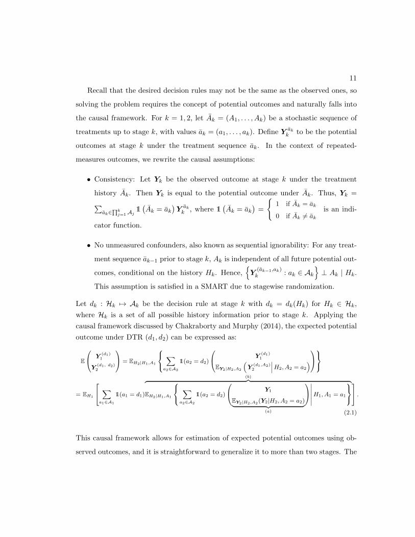
Recall that the desired decision rules may not be the same as the observed ones, so

solving the problem requires the concept of potential outcomes and naturally falls into

the causal framework. For k = 1, 2, let Ak = (A1, . . . , Ak) be a stochastic sequence of

treatments up to stage k, with values ak = (a1, . . . , ak). Define Y akk to be the potential

outcomes at stage k under the treatment sequence ak. In the context of repeated-

measures outcomes, we rewrite the causal assumptions:

• Consistency: Let Yk be the observed outcome at stage k under the treatment

history Ak. Then Yk is equal to the potential outcome under Ak. Thus, Yk =∑ak∈

∏kj=1Aj

1(Ak = ak

)Y akk , where 1

(Ak = ak

)=

{1 if Ak = ak

0 if Ak 6= akis an indi-

cator function.

• No unmeasured confounders, also known as sequential ignorability: For any treat-

ment sequence ak−1 prior to stage k, Ak is independent of all future potential out-

comes, conditional on the history Hk. Hence,{Y

(ak−1,ak)k : ak ∈ Ak

}⊥ Ak | Hk.

This assumption is satisfied in a SMART due to stagewise randomization.

Let dk : Hk 7→ Ak be the decision rule at stage k with dk = dk(Hk) for Hk ∈ Hk,where Hk is a set of all possible history information prior to stage k. Applying the

causal framework discussed by Chakraborty and Murphy (2014), the expected potential

outcome under DTR (d1, d2) can be expressed as:

E

Y(d1)1

Y(d1, d2)2

= EH2|H1,A1

∑a2∈A2

1(a2 = d2)

Y(d1)1

EY2|H2,A2

(Y

(d1,A2)2

∣∣∣H2, A2 = a2

)

= EH1

∑a1∈A1

1(a1 = d1)

(b)︷︸︸︷EH2|H1,A1

∑a2∈A2

1(a2 = d2)

Y1

EY2|H2,A2(Y2|H2, A2 = a2)︸︷︷︸

(a)

∣∣∣∣∣∣H1, A1 = a1

.

(2.1)

This causal framework allows for estimation of expected potential outcomes using ob-

served outcomes, and it is straightforward to generalize it to more than two stages. The

12

doubly-iterated expectation in Equation (2.1) provides a mathematical guidance for im-

plementing Q-learning. Here, (a) and (b) are the key estimands and will be used to

construct estimands to address the scientific problems of interest. We will discuss these

estimands in greater detail in Section 2.2.2. The vector nature of Y1 and Y2 inspires

the use of GEE techniques (Zeger and Liang, 1986) to estimate them, which will be

discussed in Section 2.3.

2.2.2 Optimization Problem

There are four main scientific problems we would like to address in this chapter: (1)

to identify the optimal decision rule at each stage as a function of the history prior

to that stage, (2) to estimate the optimal trajectory over time, (3) to estimate the

heterogeneous causal effects of stage 2 treatment over time, conditional on the history

prior to stage 2, and (4) to estimate the heterogeneous causal effects of stage 1 treatment

over time, provided that participants follow the optimal treatment at stage 2. Note

that the outcome of interest is formed by a sequence of vectors, and it is impossible

to minimize a vector without any partial orders. Scientifically, the importance of these

outcomes may vary based on the time of measurement, and it is for clinical investigators

to decide. Thus, we assign weights wk to each Yk, k = 1, 2, where elements of wk are

nonnegative, and the scalar2∑

k=1

wTk Yk is the target of optimization. Since outcomes

with smaller magnitude are more desirable in the M-bridge study and elements of wk

are nonnegative, smaller values of

2∑k=1

wTk Yk are preferred.

The underlying estimands in the above-mentioned scientific problems can be ex-

pressed using (a) and (b). We restrict the problem in the comparison between two

available treatments at a specific stage, as described in the M-bridge study. The frame-

work can be generalizable to multiple treatment options, with treatment effects defined

through pairwise comparison and contrasts.

Conditional on the history prior to stage 2, the heterogeneous causal effects, also

13

known as conditional average treatment effects (CATE) (Abrevaya et al., 2015), or

moderated causal effects (Wodtke and Almirall, 2017) of stage 2 treatment over time,

are defined as

τ2(H2) = E(Y2|H2, A2 = 1)− E(Y2|H2, A2 = −1). (2.2)

Therefore, the optimal treatment rule at stage 2 is dopt2 (H2) = −sgn

{wT

2 τ2(H2)}

, where

sgn(x) =

{−1 if x < 0

1 otherwise.

Suppose the subjects follow the optimal treatment at stage 2, the heterogeneous

causal effects of stage 1 treatment over time is defined as

τ1(H1) = E

Y1

E(Y2

∣∣H2, A2 = dopt2

)∣∣∣∣∣∣H1, A1 = 1

−E

Y1

E(Y2

∣∣H2, A2 = dopt2

)∣∣∣∣∣∣H1, A1 = −1

,

(2.3)

and hence the optimal treatment rule at stage 1 is dopt1 (H1) = −sgn

{(wT

1 wT2

)τ1(H1)

}.

The marginal optimal trajectory is obtained by substituting d1 = dopt1 (H1) and

d2 = dopt2 (H2) in Equation (2.1).

2.3 Modified Q-learning with Generalized Estimating Equa-

tions

Q-learning is a widely implemented algorithm to identify the optimal DTR. It is also

discussed in literature (Huang et al., 2015) that the expected trajectory of embedded

treatment regimes can be estimated as a by-product of Q-learning. Instead of speci-

fying a simple linear regression for each Q-function, we propose to utilize a marginal

model that can generate point estimates at all measurement times. GEE techniques

are then used to estimate the model parameters, taking advantage of the robustness to

misspecification of working covariance matrix.

14

2.3.1 Composite Q-learning

Suppose (Z1i, A1i,Y1i, Z2i, A2i,Y2i) is the sample data collected for subject i, i =

1, . . . , n. In order to apply the standard Q-learning algorithm, we could collapse repeated-

measures outcomes using a weighted sum, and the Q-functions are defined as:

Q2(H2i, A2i) = E(wT

2 Y2i

∣∣H2i, A2i

),

Q1(H1i, A1i) = E(wT

1 Y1i +Q2

(H2i, A2i = dopt

2

)∣∣∣H1i, A1i

), (2.4)

where wk is a clinically specified weight vector for outcomes at stage k, as described in

Section 2.2.2. Consider Q-functions of the parametric form

Qk(Hki, Aki;βk,ψk) = xTk0,iβk +AkixTk1,iψk, k = 1, 2, (2.5)

where xk0,i and xk1,i are realizations of functions of Hki. Starting from stage 2, β2 and

ψ2, are obtained using least squares estimation. Stage 1 estimators, β1 and ψ1, are

estimated by regressing wT1 Y1 + min

a2∈{−1,1}Q2

(H2, A2 = a2; β1, ψ1

)on H1 and A1. We

term this type of Q-learning as composite Q-learning.

2.3.2 Q-learning with Generalized Estimating Equations

Our proposed method does not collapse repeated-measures outcomes but treats repeated-

measures outcomes as a vector. Let tk = (tk1 . . . tkj . . . tkJk)T be a vector of all mea-

surement times right after the treatment period at stage k, including measurements at

future stages. Throughout the chapter, we assume that measurements are taken at the

same time across subjects. Therefore, the Q-functions are re-defined as

Q2(H2i, A2i, t2) = E (Y2i|H2i, A2i) ,

Q1(H1i, A1i, t1) = E

Y1i

Q2

(H2i, A2i = dopt

2i , t2

)∣∣∣∣∣∣H1i, A1i

. (2.6)

15

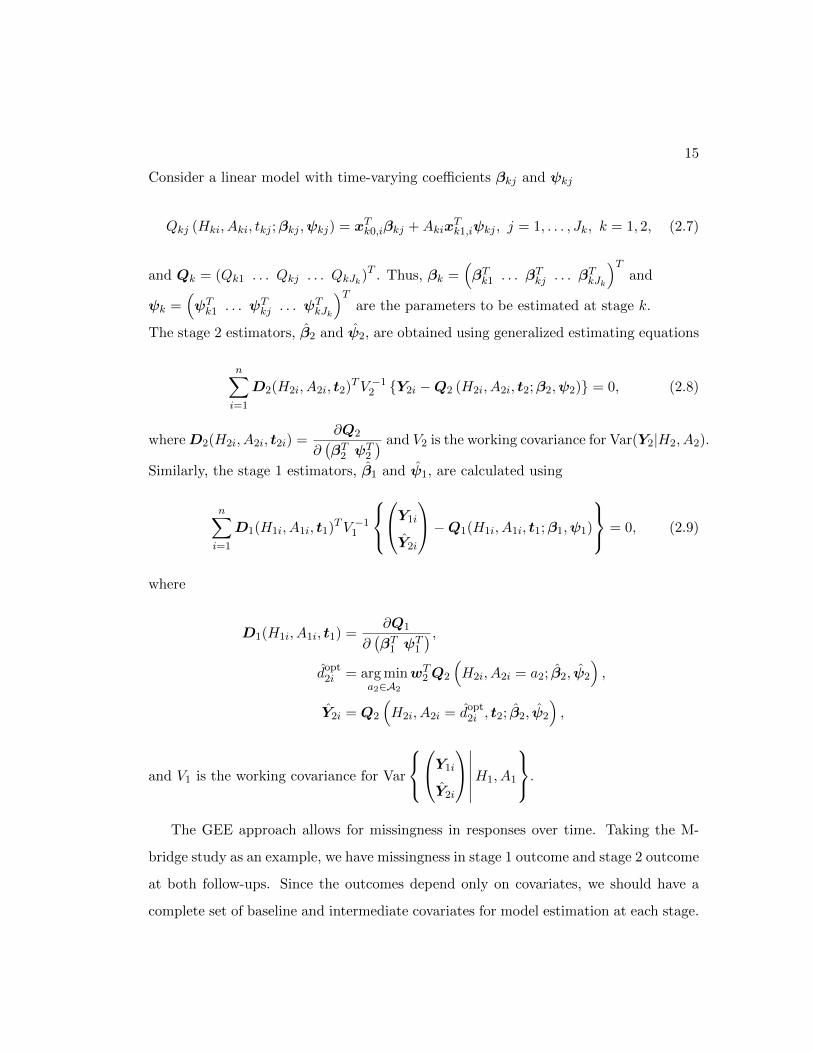
Consider a linear model with time-varying coefficients βkj and ψkj

Qkj (Hki, Aki, tkj ;βkj ,ψkj) = xTk0,iβkj +AkixTk1,iψkj , j = 1, . . . , Jk, k = 1, 2, (2.7)

and Qk = (Qk1 . . . Qkj . . . QkJk)T . Thus, βk =(βTk1 . . . βTkj . . . β

TkJk

)Tand

ψk =(ψTk1 . . . ψTkj . . . ψ

TkJk

)Tare the parameters to be estimated at stage k.

The stage 2 estimators, β2 and ψ2, are obtained using generalized estimating equations

n∑i=1

D2(H2i, A2i, t2)TV −12 {Y2i −Q2 (H2i, A2i, t2;β2,ψ2)} = 0, (2.8)

whereD2(H2i, A2i, t2i) =∂Q2

∂(βT2 ψ

T2

) and V2 is the working covariance for Var(Y2|H2, A2).

Similarly, the stage 1 estimators, β1 and ψ1, are calculated using

n∑i=1

D1(H1i, A1i, t1)TV −11

Y1i

Y2i

−Q1(H1i, A1i, t1;β1,ψ1)

= 0, (2.9)

where

D1(H1i, A1i, t1) =∂Q1

∂(βT1 ψ

T1

) ,dopt

2i = arg mina2∈A2

wT2 Q2

(H2i, A2i = a2; β2, ψ2

),

Y2i = Q2

(H2i, A2i = dopt

2i , t2; β2, ψ2

),

and V1 is the working covariance for Var

Y1i

Y2i

∣∣∣∣∣∣H1, A1

.

The GEE approach allows for missingness in responses over time. Taking the M-

bridge study as an example, we have missingness in stage 1 outcome and stage 2 outcome

at both follow-ups. Since the outcomes depend only on covariates, we should have a

complete set of baseline and intermediate covariates for model estimation at each stage.

16

An issue with respect to the estimation procedure in Q-learning is that stage 2 outcome

depends on stage 1 outcome. Hence, missingness in stage 1 outcome causes problems in

stage 2 estimation. The design of the M-bridge study obviates this issue by introducing

the tailoring variable. The tailoring variable, whether the students were flagged as

heavy drinkers, is defined based on the stage 1 outcome, and those with missing stage

1 outcomes were not flagged as heavy drinkers. Since only heavy drinkers were re-

randomized at stage 2, the students we include in stage 2 estimation all have complete

covariate data.

In practice, choosing a wrong working structure for V1 and V2 can raise issues in

estimation. Liang and Zeger (1986) argued that there was little difference in estimation

of parameters when the true correlation was moderate. Zhao et al. (1992) claimed that

wrong specification of an independent correlation matrix when outcomes were strongly

dependent would result in “important losses of efficiency”, as compared to the smaller

reduction in efficiency when specifying unnecessary high correlations. In the presence of

missingness not completely at random, Fitzmaurice et al. (1993) advocated for obtaining

a close approximation to the covariance structure in outcomes so that the estimators of

time-dependent treatment effects were substantially less biased. SMARTs usually result

in a balanced design with time-invariant covariates. Moreover, the M-bridge study has

relatively few repeated measures at each stage. Considering all these arguments, we

recommend an unstructured working correlation structure.

The estimands discussed in Section 2.2.2 can now be written as functions of pa-

rameter estimates. The estimated optimal decision rule at stage k for individual i is

identified by minimizing a weighted sum of Q-functions at stage k:

dopt2i = arg min

a2∈A2

wT2 Q2

(H2i, A2i = a2; β2, ψ2

),

dopt1i = arg min

a1∈A1

(wT

1 wT2

)Q1

(H1i, A1i = a1; β1, ψ1

). (2.10)

The estimated heterogeneous causal effects at times of interest following the stage k

17

treatment period are calculated as:

τk(Hk) = Qk

(Hk, Ak = 1, tk; βk, ψk

)−Qk

(Hk, Ak = −1, tk; βk, ψk

), k = 1, 2.

(2.11)

2.3.3 Modified Q-learning with Murphy’s Regret Function

Model misspecification is a common issue in the implementation of Q-learning. Q-

learning requires models at all stages to be correctly specified for consistent estimation

of the optimal DTR and heterogeneous causal effects. In this thesis, we assume that the

treatment effect models are correctly specified. Backward induction features multi-stage

analysis, so even without any unmeasured confounders, misspecification of main effect

model at a later stage can bias the estimation of treatment effects at earlier stages, thus

resulting in an adverse impact on identification of the optimal DTR and the estimation

of the optimal trajectory. Because the focus of the stage 2 model is on the estimation

of the stage 2 heterogeneous causal effects, the interaction between baseline covariates

and stage 1 treatment may be overlooked in the stage 2 model. Not adjusting for some

important interactions in the stage 2 model and only including them in the stage 1 model

will result in biased stage 1 treatment effect estimators. In the example of M-bridge, it

is more difficult to select correct Z1 ∗A1 interactions into stage 2 model a priori due to

the large number of baseline covariates that the study is considering. Thus, we would

like to introduce some robustness to our proposed method by borrowing the concept of

modified Q-learning (Huang et al., 2015).

The modified version of composite Q-learning defines the Q-function at stage 1 as

Q1(H1i, A1i) = E(wT

1 Y1i +wT2 Y2i + ∆2i

∣∣H1i, A1i

), (2.12)

18

where ∆2i is the Murphy’s regret function at stage 2 and

∆2i =

0 if A2i = dopt2i

−2∣∣∣xT21,iψ2

∣∣∣ if A2i 6= dopt2i

.

Thus, the stage 1 estimators in modified composite Q-learning are obtained by regressing

wT1 Y1 +wT

2 Y2i − 2∣∣∣xT21,iψ2

∣∣∣1{A2i 6= dopt2i

}on H1 and A1.

Applying this technique to Q-learning with GEE, our proposed modification to the

algorithm illustrated in Section 2.3.2 updates stage 1 Q-function (2.6) as

Q1(H1i, A1i) = E

Y1i

Y2i + ∆2i

∣∣∣∣∣∣H1i, A1i

, (2.13)

where

∆2i =

0 if A2i = dopt2i

dopt2i τ2(H2i) if A2i 6= dopt

2i

.

Thus, the stage 1 estimators in modified Q-learning with GEE are obtained using Equa-

tion (2.9) with Y2i = Y2i + dopt2i τ2(H2i)1

{A2i 6= dopt

2i

}. This approach makes as much

use of observations as possible and is robust to misspecification of stage 2 main effect

model.

2.4 Simulation Study

In this section, we present a simulation study to compare the performance of the four

methods illustrated in Section 3.5: (1) composite Q-learning (Q), (2) modified composite

Q-learning (mQ), (3) Q-learning with GEE (Q-GEE), and (4) modified Q-learning with

GEE (mQ-GEE).

19

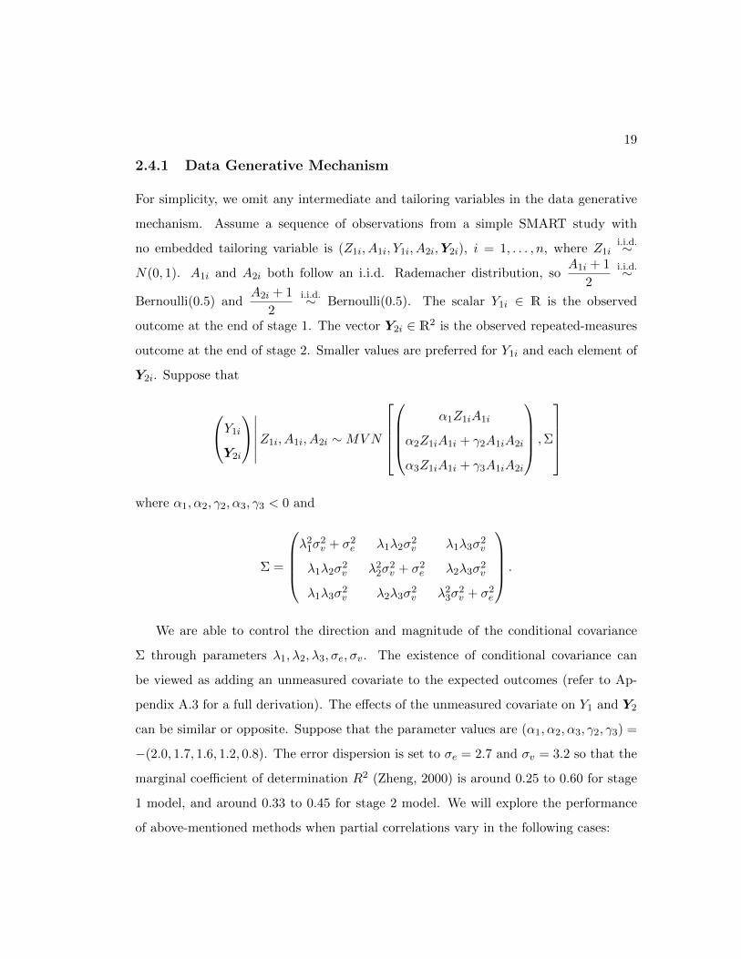
2.4.1 Data Generative Mechanism

For simplicity, we omit any intermediate and tailoring variables in the data generative

mechanism. Assume a sequence of observations from a simple SMART study with

no embedded tailoring variable is (Z1i, A1i, Y1i, A2i,Y2i), i = 1, . . . , n, where Z1ii.i.d.∼

N(0, 1). A1i and A2i both follow an i.i.d. Rademacher distribution, soA1i + 1

2

i.i.d.∼

Bernoulli(0.5) andA2i + 1

2

i.i.d.∼ Bernoulli(0.5). The scalar Y1i ∈ R is the observed

outcome at the end of stage 1. The vector Y2i ∈ R2 is the observed repeated-measures

outcome at the end of stage 2. Smaller values are preferred for Y1i and each element of

Y2i. Suppose that

Y1i

Y2i

∣∣∣∣∣∣Z1i, A1i, A2i ∼MVN

α1Z1iA1i

α2Z1iA1i + γ2A1iA2i

α3Z1iA1i + γ3A1iA2i

,Σ

where α1, α2, γ2, α3, γ3 < 0 and

Σ =

λ2

1σ2v + σ2

e λ1λ2σ2v λ1λ3σ

2v

λ1λ2σ2v λ2

2σ2v + σ2

e λ2λ3σ2v

λ1λ3σ2v λ2λ3σ

2v λ2

3σ2v + σ2

e

.

We are able to control the direction and magnitude of the conditional covariance

Σ through parameters λ1, λ2, λ3, σe, σv. The existence of conditional covariance can

be viewed as adding an unmeasured covariate to the expected outcomes (refer to Ap-

pendix A.3 for a full derivation). The effects of the unmeasured covariate on Y1 and Y2

can be similar or opposite. Suppose that the parameter values are (α1, α2, α3, γ2, γ3) =

−(2.0, 1.7, 1.6, 1.2, 0.8). The error dispersion is set to σe = 2.7 and σv = 3.2 so that the

marginal coefficient of determination R2 (Zheng, 2000) is around 0.25 to 0.60 for stage

1 model, and around 0.33 to 0.45 for stage 2 model. We will explore the performance

of above-mentioned methods when partial correlations vary in the following cases:

20

(I) Y1 and Y2 are not conditionally correlated, λ1 = λ2 = λ3 = 0.

(II) Y1 and Y2 are positively conditionally correlated, λ1 = λ2 = λ3 = 1.

(III) Y1 and Y2 are negatively conditionally correlated, λ1 = 1 and λ2 = λ3 = −1.

2.4.2 Evaluation Criteria

Three metrics are defined to assess the consistency and efficiency of doptk and τ1:

(1) PCIk =1

n

n∑i=1

1{doptki = dopt

ki

}: the probability of correctly identified optimal rules

(PCI) at stage k, where doptki is the estimated optimal decision rule at stage k

for subject i using Equation (2.10) with elements of Qk being equally weighted,

and doptki is the true optimal decision rule at stage k for subject i, minimizing the

averaged outcomes following stage k treatment.

(2) RMSEτ1j =

[1

n

n∑i=1

{τ1j(Z1i)− τ1j(Z1i)

}2]1/2

: root mean square error (RMSE)

of the estimated heterogeneous causal effects of stage 1 treatment at the jth

measurement, j = 1, 2, 3, assuming participants follow the optimal treatment at

stage 2. τ1j(Z1i) is the jth element of τ1 from Equation (2.11).

(3) Biasτ1j(Z1) = τ1j(Z1) − τ1j(Z1) for a grid of values Z1, where τ1j(Z1) is the jth

element of τ1 from Equation (2.3).

RMSE is the standard deviation of prediction errors. RMSEτ1j provides information

on both accuracy and efficiency of using the stage 1 model to estimate heterogeneous

causal effects across samples, and measures how accurate and precise the predicted

heterogeneous causal effects are to the true values of the estimands over a sample of

participants. Biasτ1j(Z1) is composed of two components: (1) the bias from the estima-

tion of stage 2 optimal rule, and (2) the bias from the estimation of stage 1 parameters.

Bias should be heterogeneous across participants and dependent on the value of baseline

measurement Z1.

21

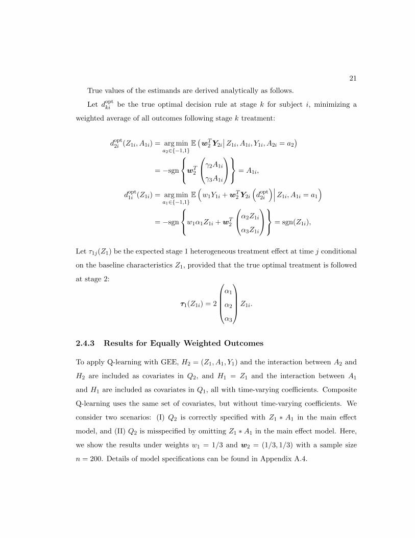
True values of the estimands are derived analytically as follows.

Let doptki be the true optimal decision rule at stage k for subject i, minimizing a

weighted average of all outcomes following stage k treatment:

dopt2i (Z1i, A1i) = arg min

a2∈{−1,1}E(wT

2 Y2i

∣∣Z1i, A1i, Y1i, A2i = a2

)= −sgn

wT2

γ2A1i

γ3A1i

= A1i,

dopt1i (Z1i) = arg min

a1∈{−1,1}E(w1Y1i +wT

2 Y2i

(dopt

2i

)∣∣∣Z1i, A1i = a1

)

= −sgn

w1α1Z1i +wT2

α2Z1i

α3Z1i

= sgn(Z1i),

Let τ1j(Z1) be the expected stage 1 heterogeneous treatment effect at time j conditional

on the baseline characteristics Z1, provided that the true optimal treatment is followed

at stage 2:

τ1(Z1i) = 2

α1

α2

α3

Z1i.

2.4.3 Results for Equally Weighted Outcomes

To apply Q-learning with GEE, H2 = (Z1, A1, Y1) and the interaction between A2 and

H2 are included as covariates in Q2, and H1 = Z1 and the interaction between A1

and H1 are included as covariates in Q1, all with time-varying coefficients. Composite

Q-learning uses the same set of covariates, but without time-varying coefficients. We

consider two scenarios: (I) Q2 is correctly specified with Z1 ∗ A1 in the main effect

model, and (II) Q2 is misspecified by omitting Z1 ∗A1 in the main effect model. Here,

we show the results under weights w1 = 1/3 and w2 = (1/3, 1/3) with a sample size

n = 200. Details of model specifications can be found in Appendix A.4.

22

2.4.3.1 Scenario I: no model misspecification

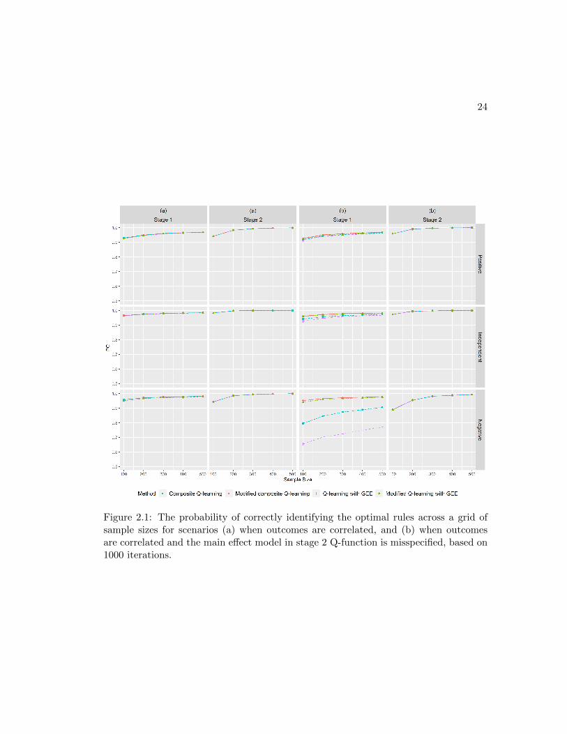
As shown in Table 2.1 and Figure 2.1(a), there is a tiny loss in the accuracy of identifying

stage 1 optimal rules using Q-learning with GEE as compared to composite Q-learning.

The loss is likely due to the additional time-varying coefficients in the marginal model

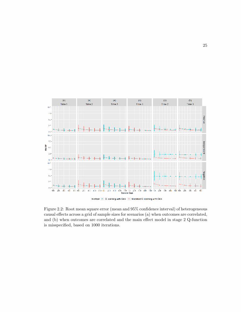
that Q-GEE has to estimate and is negligible considering the high accuracy. Q-lGEE

is able to estimate heterogeneous causal effects (Table 2.1 and Figure 2.2(a)), and the

modified version of Q-GEE has exactly the same performance as the standard algorithm.

Partial Correlation Method PCI1 PCI2 RMSEτ11 RMSEτ12 RMSEτ13

Positive

Q 0.950 0.983 - - -mQ 0.950 0.983 - - -

Q-GEE 0.947 0.983 0.74 (0.38) 0.97 (0.52) 0.94 (0.49)mQ-GEE 0.947 0.983 0.74 (0.38) 0.97 (0.52) 0.94 (0.49)

Independent

Q 0.976 0.998 - - -mQ 0.976 0.998 - - -

Q-GEE 0.974 0.998 0.49 (0.26) 0.69 (0.36) 0.68 (0.35)mQ-GEE 0.974 0.998 0.49 (0.26) 0.69 (0.36) 0.68 (0.35)

Negative

Q 0.970 0.984 - - -mQ 0.970 0.984 - - -

Q-GEE 0.966 0.984 0.74 (0.38) 0.98 (0.51) 0.94 (0.51)mQ-GEE 0.966 0.984 0.74 (0.38) 0.98 (0.51) 0.94 (0.51)

Table 2.1: (Scenario I) PCI of optimal rules and RMSE (mean (SD)) of estimated het-erogeneous causal effects, based on estimated stage 1 Q-functions from 1000 simulationswith sample size n = 200.

2.4.3.2 Scenario II: misspecified stage 2 main effect model

Under this circumstance, mQ-GEE universally outperforms Q-GEE in PCI1 (Table 2.2

and Figure 2.1(b)), the RMSE of predicting heterogeneous causal effects (Table 2.2 and

Figure 2.2(b)), and the bias of estimating heterogeneous causal effects based on a grid

of Z1 values (Figure 2.3(b)). This confirms our hypothesis that modified Q-learning

avoids bias caused by misspecification of stage 2 main effect model. For more extreme

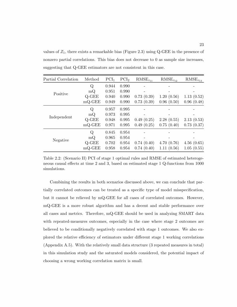
23

values of Z1, there exists a remarkable bias (Figure 2.3) using Q-GEE in the presence of

nonzero partial correlations. This bias does not decrease to 0 as sample size increases,

suggesting that Q-GEE estimators are not consistent in this case.


Positive

Q 0.944 0.990 - - -mQ 0.951 0.990 - - -

Q-GEE 0.940 0.990 0.73 (0.39) 1.20 (0.56) 1.13 (0.52)mQ-GEE 0.949 0.990 0.73 (0.39) 0.96 (0.50) 0.96 (0.48)

Independent

Q 0.957 0.995 - - -mQ 0.973 0.995 - - -

Q-GEE 0.948 0.995 0.49 (0.25) 2.28 (0.55) 2.13 (0.53)mQ-GEE 0.971 0.995 0.49 (0.25) 0.75 (0.40) 0.73 (0.37)

Negative

Q 0.845 0.954 - - -mQ 0.965 0.954 - - -

Q-GEE 0.702 0.954 0.74 (0.40) 4.70 (0.76) 4.56 (0.65)mQ-GEE 0.958 0.954 0.74 (0.40) 1.11 (0.56) 1.05 (0.55)

Table 2.2: (Scenario II) PCI of stage 1 optimal rules and RMSE of estimated heteroge-neous causal effects at time 2 and 3, based on estimated stage 1 Q-functions from 1000simulations.

Combining the results in both scenarios discussed above, we can conclude that par-

tially correlated outcomes can be treated as a specific type of model misspecification,

but it cannot be relieved by mQ-GEE for all cases of correlated outcomes. However,

mQ-GEE is a more robust algorithm and has a decent and stable performance over

all cases and metrics. Therefore, mQ-GEE should be used in analyzing SMART data

with repeated-measures outcomes, especially in the case where stage 2 outcomes are

believed to be conditionally negatively correlated with stage 1 outcomes. We also ex-

plored the relative efficiency of estimators under different stage 1 working correlations

(Appendix A.5). With the relatively small data structure (3 repeated measures in total)

in this simulation study and the saturated models considered, the potential impact of

choosing a wrong working correlation matrix is small.

24

Figure 2.1: The probability of correctly identifying the optimal rules across a grid ofsample sizes for scenarios (a) when outcomes are correlated, and (b) when outcomesare correlated and the main effect model in stage 2 Q-function is misspecified, based on1000 iterations.

25

Figure 2.2: Root mean square error (mean and 95% confidence interval) of heterogeneouscausal effects across a grid of sample sizes for scenarios (a) when outcomes are correlated,and (b) when outcomes are correlated and the main effect model in stage 2 Q-functionis misspecified, based on 1000 iterations.

26

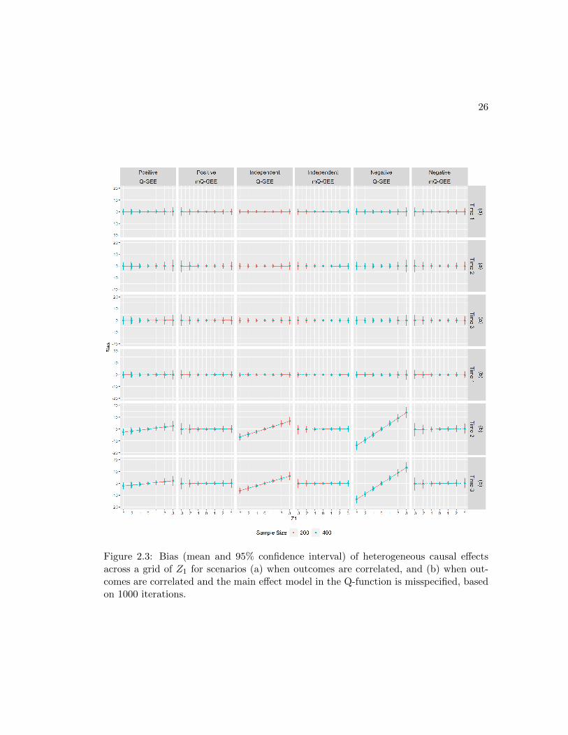
Figure 2.3: Bias (mean and 95% confidence interval) of heterogeneous causal effectsacross a grid of Z1 for scenarios (a) when outcomes are correlated, and (b) when out-comes are correlated and the main effect model in the Q-function is misspecified, basedon 1000 iterations.

27

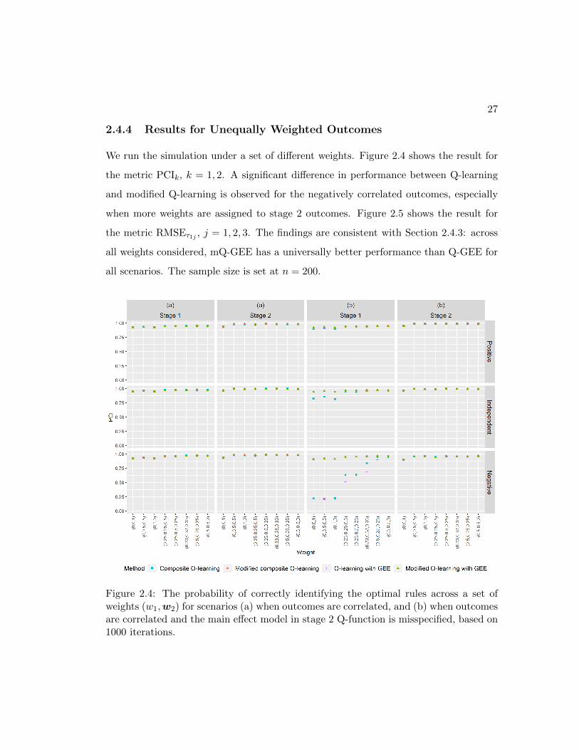
2.4.4 Results for Unequally Weighted Outcomes

We run the simulation under a set of different weights. Figure 2.4 shows the result for

the metric PCIk, k = 1, 2. A significant difference in performance between Q-learning

and modified Q-learning is observed for the negatively correlated outcomes, especially

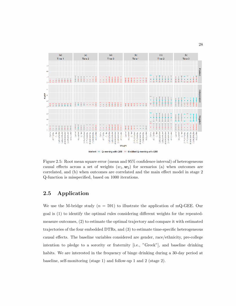
when more weights are assigned to stage 2 outcomes. Figure 2.5 shows the result for

the metric RMSEτ1j , j = 1, 2, 3. The findings are consistent with Section 2.4.3: across

all weights considered, mQ-GEE has a universally better performance than Q-GEE for

all scenarios. The sample size is set at n = 200.

Figure 2.4: The probability of correctly identifying the optimal rules across a set ofweights (w1,w2) for scenarios (a) when outcomes are correlated, and (b) when outcomesare correlated and the main effect model in stage 2 Q-function is misspecified, based on1000 iterations.

28

Figure 2.5: Root mean square error (mean and 95% confidence interval) of heterogeneouscausal effects across a set of weights (w1,w2) for scenarios (a) when outcomes arecorrelated, and (b) when outcomes are correlated and the main effect model in stage 2Q-function is misspecified, based on 1000 iterations.

2.5 Application

We use the M-bridge study (n = 591) to illustrate the application of mQ-GEE. Our

goal is (1) to identify the optimal rules considering different weights for the repeated-

measure outcomes, (2) to estimate the optimal trajectory and compare it with estimated

trajectories of the four embedded DTRs, and (3) to estimate time-specific heterogeneous

causal effects. The baseline variables considered are gender, race/ethnicity, pre-college

intention to pledge to a sorority or fraternity [i.e., ”Greek”], and baseline drinking

habits. We are interested in the frequency of binge drinking during a 30-day period at

baseline, self-monitoring (stage 1) and follow-up 1 and 2 (stage 2).

29

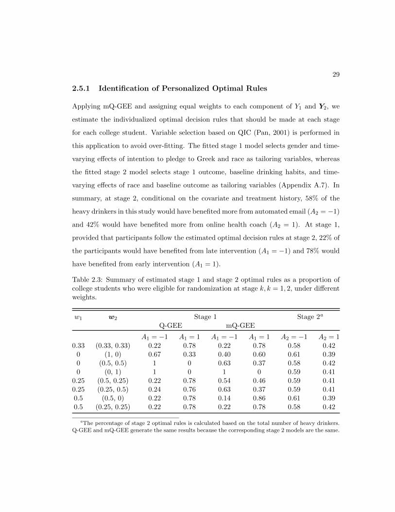
2.5.1 Identification of Personalized Optimal Rules

Applying mQ-GEE and assigning equal weights to each component of Y1 and Y2, we

estimate the individualized optimal decision rules that should be made at each stage

for each college student. Variable selection based on QIC (Pan, 2001) is performed in

this application to avoid over-fitting. The fitted stage 1 model selects gender and time-

varying effects of intention to pledge to Greek and race as tailoring variables, whereas

the fitted stage 2 model selects stage 1 outcome, baseline drinking habits, and time-

varying effects of race and baseline outcome as tailoring variables (Appendix A.7). In

summary, at stage 2, conditional on the covariate and treatment history, 58% of the

heavy drinkers in this study would have benefited more from automated email (A2 = −1)

and 42% would have benefited more from online health coach (A2 = 1). At stage 1,

provided that participants follow the estimated optimal decision rules at stage 2, 22% of

the participants would have benefited from late intervention (A1 = −1) and 78% would

have benefited from early intervention (A1 = 1).

Table 2.3: Summary of estimated stage 1 and stage 2 optimal rules as a proportion ofcollege students who were eligible for randomization at stage k, k = 1, 2, under differentweights.

w1 w2 Stage 1 Stage 2a

Q-GEE mQ-GEE

A1 = −1 A1 = 1 A1 = −1 A1 = 1 A2 = −1 A2 = 10.33 (0.33, 0.33) 0.22 0.78 0.22 0.78 0.58 0.42

0 (1, 0) 0.67 0.33 0.40 0.60 0.61 0.390 (0.5, 0.5) 1 0 0.63 0.37 0.58 0.420 (0, 1) 1 0 1 0 0.59 0.41

0.25 (0.5, 0.25) 0.22 0.78 0.54 0.46 0.59 0.410.25 (0.25, 0.5) 0.24 0.76 0.63 0.37 0.59 0.410.5 (0.5, 0) 0.22 0.78 0.14 0.86 0.61 0.390.5 (0.25, 0.25) 0.22 0.78 0.22 0.78 0.58 0.42

aThe percentage of stage 2 optimal rules is calculated based on the total number of heavy drinkers.Q-GEE and mQ-GEE generate the same results because the corresponding stage 2 models are the same.

30

We also explored the performance of Q-GEE and mQ-GEE under different weights.

Table 2.3 shows a summary of the results. The assignment of stage 2 optimal rule is

similar for both methods. However, it seems that mQ-GEE is more sensitive to the

change in weights.

2.5.2 Point Estimation of the Optimal Trajectory and Heterogeneous

Causal Effects

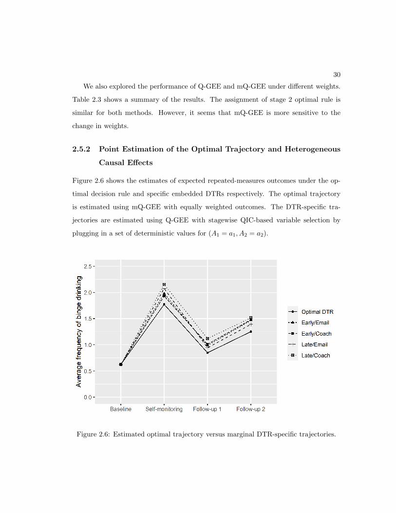
Figure 2.6 shows the estimates of expected repeated-measures outcomes under the op-

timal decision rule and specific embedded DTRs respectively. The optimal trajectory

is estimated using mQ-GEE with equally weighted outcomes. The DTR-specific tra-

jectories are estimated using Q-GEE with stagewise QIC-based variable selection by

plugging in a set of deterministic values for (A1 = a1, A2 = a2).

Figure 2.6: Estimated optimal trajectory versus marginal DTR-specific trajectories.

31

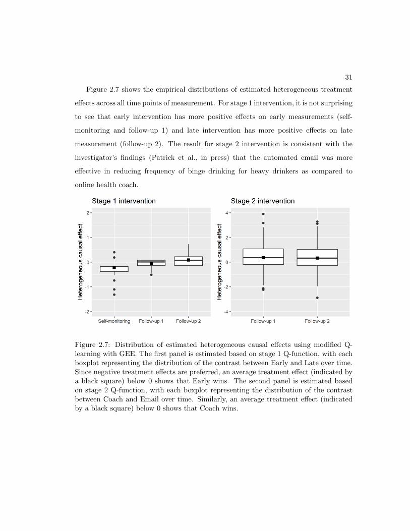
Figure 2.7 shows the empirical distributions of estimated heterogeneous treatment

effects across all time points of measurement. For stage 1 intervention, it is not surprising

to see that early intervention has more positive effects on early measurements (self-

monitoring and follow-up 1) and late intervention has more positive effects on late

measurement (follow-up 2). The result for stage 2 intervention is consistent with the

investigator’s findings (Patrick et al., in press) that the automated email was more

effective in reducing frequency of binge drinking for heavy drinkers as compared to

online health coach.

Figure 2.7: Distribution of estimated heterogeneous causal effects using modified Q-learning with GEE. The first panel is estimated based on stage 1 Q-function, with eachboxplot representing the distribution of the contrast between Early and Late over time.Since negative treatment effects are preferred, an average treatment effect (indicated bya black square) below 0 shows that Early wins. The second panel is estimated basedon stage 2 Q-function, with each boxplot representing the distribution of the contrastbetween Coach and Email over time. Similarly, an average treatment effect (indicatedby a black square) below 0 shows that Coach wins.

32

2.6 Discussion

We developed an implementation of Q-learning on stagewise repeated-measures out-

comes using generalized estimating equations. To apply the proposed method, inves-

tigators have the flexibility to choose science-driven weights for the repeated-measures

outcomes. For implementing GEE, we recommend specifying unstructured working

correlation, because in conventional SMARTs, participants are followed a considerably

small number of times before the next stage of re-randomization or the end of study,

and sample size is comparatively large. Furthermore, by using a saturated marginal

model with time-varying coefficients, the impact of choosing a wrong working correla-

tion is negligible. We also explored the performance of the proposed method in terms of

rule identification and the consistency and efficiency of estimating heterogeneous causal

effects. The performance of regression-based Q-learning depends heavily on correct

specification of models at all stages. The modified version of Q-learning with GEE

mitigates the problem by incorporating the residual from observed outcomes at subse-

quent stages into the pseudo-outcome at previous stages. This thesis focuses only on

point estimation of the optimal trajectory. Inference under nonregularity conditions,

where the weighted stage 2 treatment effect equals to 0, can be a complex problem that

needs further research. Moreover, future work needs to be done to extend the proposed

method for discrete outcomes, e.g., dichotomous responses which many investigators

care about in clinical trials.

Chapter 3

On the Model Misspecification in

Q-learning with Treatment Effect

Heterogeneity

3.1 Literature Review

Q-learning with linear regression (Murphy, 2005b; Nahum-Shani et al., 2012) is a widely

used backward induction algorithm to identify the optimal DTR due to its ease of

implementation. At each stage of randomization, Q-learning specifies a Q-function, a

parametric model of the expected pseudo-outcomes conditional on past history, where

the pseudo-outcomes are the potential outcomes assuming that the optimal interventions

are followed thereafter. Typically in practice, one specifies the Q-function as a linear

model, which consists of a main effect model and a treatment effect model, and the

model parameters are usually estimated using least squares estimation. The main effect

component characterizes the variation in the outcome that is explained by pre-treatment

covariates, whereas the treatment effect component characterizes the average effect of

the observed treatment allowing for variation with pre-treatment covariates.

33

34

Decision making at a single stage, for example, using data from a randomized con-

trolled trial, does not depend on the main effect model, as the treatment effect model

fully defines the estimated optimal rule. However, this is not the case for backward

induction over multiple stages. The performance of Q-learning is susceptible to model

misspecification of the main effect model. Heterogeneous treatment effects at an earlier

stage on a final outcome are in fact part of the main effects at later stages (either the

earlier treatment-covariate interaction or an intermediate measurement which depends

on prior treatement). It is reasonable to conjecture that omitting them at later stages

would result in biased estimation of the treatment effects at early stages. This is an

example of informative residual bias in optimizing over multiple stages.

Additionally, heterogeneous treatment effects at a later stage result in biased estima-

tion if linear models are used in earlier stages as the optimization operation necessarily

makes the linearity misspecified. Though the treatment effect model of a Q-function

is assumed to be correctly specified with no unmeasured confounders, a nonlinear re-

lationship between the predictors and the pseudo-outcome, which usually involves an

absolute value function of the estimated treatment effects, arises inevitably when the

estimated treatment effects at late stages are heterogeneous. This problem was studied

comprehensively by Laber et al. (2014).

Both types of misspecification described above result in a nonnegligible bias in the

prediction of stage 1 optimal rules, and have been addressed with carefully constructed

methods. Existing methods that deal with residual bias are modified Q-learning (Huang

et al., 2015), A-learning (Schulte et al., 2014) and robust Q-learning (Ertefaie et al.,

2021). A-learning takes a propensity score approach and allows for flexible modeling

of the main effects. Robust Q-learning as well takes a propensity score approach, but

obviates the need to specify the main effect model. However, nonparametric methods

are usually used to estimate the main effects in A-learning and the expected outcome

in robust Q-learning. Nonparametric methods work ideally for nonlinearity between

35

outcomes and covariates, but are less straightforward when implementation and inter-

pretation come into consideration. Moreover, model checking and residual diagnostics

for Q-learning with linear regression can be easily performed using standard approaches

(Henderson et al., 2010; Chakraborty and Moodie, 2013). Therefore, we advocate the

use of modified Q-learning, a parametric approach that takes account of stage 2 residu-

als, for dealing with misspecification of the main effect model. For the treatment effect

model, Laber et al. (2014) proposed an interactive model building of Q-learning to cor-

rect the bias caused by misspecified linearity between pseudo-outcome and predictors.

The above-mentioned methods work well for one specific type of misspecification, but

fail to consider the coexistence of misspecifications as a result of heterogeneous treatment

effects. This chapter starts with an introduction of the data structure and a further

elaboration on the importance of the problem using the M-bridge study as an example.

We then discuss the integrative impact of late-stage unadjusted residuals and early-

stage nonlinearity on the prediction of optimal rules, with mathematical formulation and

proof in Section 3.4 to help understand the statistical aspects of the problem. We then

propose to build interactive models into modified parametric Q-learning with Murphy’s

regret function in Section 3.5. Simulations are performed to show the robustness of

our proposed algorithm. Finally, we demonstrate its application on SMARTs with

embedded tailoring using the M-bridge data.

3.2 Framework

3.2.1 Data Example

The data example we use to illustrate the problem omits the repeated-measures outcome

in the M-bridge design. As shown in Figure 3.1, the outcomes of interest, binge drinking

(primary outcome) and negative drinking-related consequences (secondary outcome),

were measured at the end of Semester 1 for all students. The target outcomes for

analysis in this section are the maximum number of drinks and the total number of

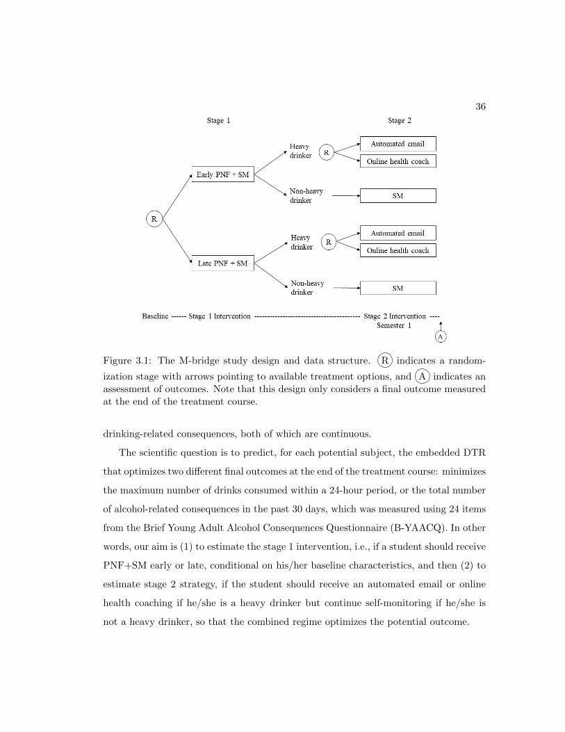
36

Figure 3.1: The M-bridge study design and data structure. R indicates a random-

ization stage with arrows pointing to available treatment options, and A indicates anassessment of outcomes. Note that this design only considers a final outcome measuredat the end of the treatment course.

drinking-related consequences, both of which are continuous.

The scientific question is to predict, for each potential subject, the embedded DTR

that optimizes two different final outcomes at the end of the treatment course: minimizes

the maximum number of drinks consumed within a 24-hour period, or the total number

of alcohol-related consequences in the past 30 days, which was measured using 24 items

from the Brief Young Adult Alcohol Consequences Questionnaire (B-YAACQ). In other

words, our aim is (1) to estimate the stage 1 intervention, i.e., if a student should receive

PNF+SM early or late, conditional on his/her baseline characteristics, and then (2) to

estimate stage 2 strategy, if the student should receive an automated email or online

health coaching if he/she is a heavy drinker but continue self-monitoring if he/she is

not a heavy drinker, so that the combined regime optimizes the potential outcome.

37

In the M-bridge study, the investigators hypothesize that pre-college alcohol use

norms and pre-college intentions for college drinking are treatment effect moderators.

These baseline variables might moderate both stage 1 and stage 2 treatment effects,

and inappropriate adjustment is likely to occur in the Q-functions at both stages as a

result of heterogeneous treatment effects. Details will be discussed in Section 3.4.

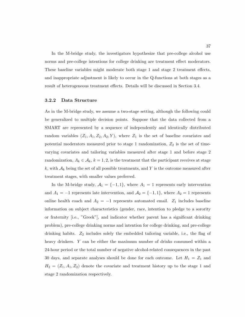
3.2.2 Data Structure

As in the M-bridge study, we assume a two-stage setting, although the following could

be generalized to multiple decision points. Suppose that the data collected from a

SMART are represented by a sequence of independently and identically distributed

random variables (Z1, A1, Z2, A2, Y ), where Z1 is the set of baseline covariates and

potential moderators measured prior to stage 1 randomization, Z2 is the set of time-

varying covariates and tailoring variables measured after stage 1 and before stage 2

randomization, Ak ∈ Ak, k = 1, 2, is the treatment that the participant receives at stage

k, with Ak being the set of all possible treatments, and Y is the outcome measured after

treatment stages, with smaller values preferred.

In the M-bridge study, A1 = {−1, 1}, where A1 = 1 represents early intervention

and A1 = −1 represents late intervention, and A2 = {−1, 1}, where A2 = 1 represents

online health coach and A2 = −1 represents automated email. Z1 includes baseline

information on subject characteristics (gender, race, intention to pledge to a sorority

or fraternity [i.e., ”Greek”], and indicator whether parent has a significant drinking

problem), pre-college drinking norms and intention for college drinking, and pre-college

drinking habits. Z2 includes solely the embedded tailoring variable, i.e., the flag of

heavy drinkers. Y can be either the maximum number of drinks consumed within a

24-hour period or the total number of negative alcohol-related consequences in the past

30 days, and separate analyses should be done for each outcome. Let H1 = Z1 and

H2 = (Z1, A1, Z2) denote the covariate and treatment history up to the stage 1 and

stage 2 randomization respectively.

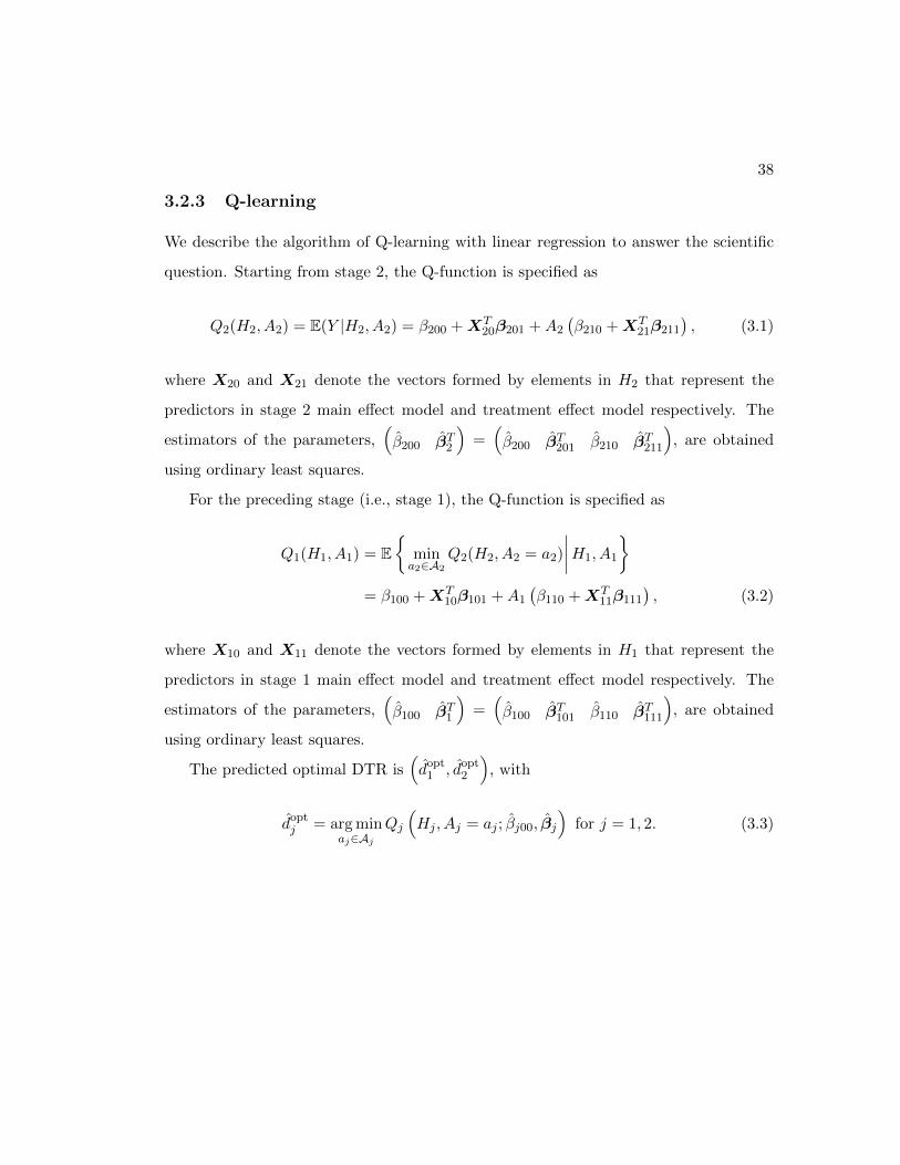
38

3.2.3 Q-learning

We describe the algorithm of Q-learning with linear regression to answer the scientific

question. Starting from stage 2, the Q-function is specified as

Q2(H2, A2) = E(Y |H2, A2) = β200 +XT20β201 +A2

(β210 +XT

21β211

), (3.1)

where X20 and X21 denote the vectors formed by elements in H2 that represent the

predictors in stage 2 main effect model and treatment effect model respectively. The

estimators of the parameters,(β200 βT2

)=(β200 βT201 β210 βT211

), are obtained

using ordinary least squares.

For the preceding stage (i.e., stage 1), the Q-function is specified as

Q1(H1, A1) = E{

mina2∈A2

Q2(H2, A2 = a2)

∣∣∣∣H1, A1

}= β100 +XT

10β101 +A1

(β110 +XT

11β111

), (3.2)

where X10 and X11 denote the vectors formed by elements in H1 that represent the

predictors in stage 1 main effect model and treatment effect model respectively. The

estimators of the parameters,(β100 βT1

)=(β100 βT101 β110 βT111

), are obtained

using ordinary least squares.

The predicted optimal DTR is(dopt

1 , dopt2

), with

doptj = arg min

aj∈Aj

Qj

(Hj , Aj = aj ; βj00, βj

)for j = 1, 2. (3.3)

39

3.3 Unmeasured Variables

3.3.1 Misspecification of Stage 2 Main Effects

To understand the problem thoroughly, we first focus on model misspecification in the

presence of an important variable prior to stage 2 randomization which is not measured

by design or omitted in the data analysis. Huang et al. (2015) argues that an unmeasured

variable causes bias in the estimation of stage 1 optimal rules and model parameters.

We briefly outline the argument here. Let V20 denote a vector of unmeasured covariates

at stage 2 that are independent of A2. We use uppercase to denote random variables

and lowercase to denote a realization of the corresponding random variable.

Suppose Y conditional on all the covariates, measured or unmeasured, has mean

E(Y |H2, A2,V20) = ψ200 + xT20ψ201 + V T20γ20 + a2

(ψ210 + xT21ψ211

)(3.4)

and variance Var(Y |H2, A2,V20) = σ22.

3.3.2 Estimation Bias

The proof of the theorems can be found in the supplementary materials.

Theorem 3.3.1 (Matrix Version of the Omitted Variable Bias Theorem). Suppose

that the true regression model for Y is Y = ψ0 + XTψ1 + V Tγ + ε, where X is a

random vector formed by measured covariates, V is formed by unmeasured covariates,

and ε ∼ N(0, σ2). The parameters associated with measured covariates, ψ ≡

ψ0

ψ1

,

are thus estimated via the misspecified model y = β0 + xTβ1 + ε∗, where y and x are

realizations of Y and X respectively. Then

E(β) ≡ E

β0

β1

= ψ +

E(V T )− E(XT )Cov(X)−1Cov(X,V )

Cov(X)−1Cov(X,V )

γ.

40

LetX2 =(XT

20 A2 A2XT21

)Tdenote the full predictor vector and assume that the

covariance matrix of X2 is invertible. By Theorem 3.3.1, E

β200

β2

=

ψ200

ψ2

+Bγ20,

where

B =

E(V T20)− E(XT

2 )Cov(X2)−1Cov(X2,V20)

Cov(X2)−1Cov(X2,V20)

. (3.5)

The first element of B corresponds to the bias associated with the intercept term and

the second element of B corresponds to the bias associated with the covariate effects.

The existence of bias in the estimation of covariate effects is then characterized by the

term Cov(X2,V20). The bias of β2 can be rewritten as

Bias(β2) = Cov(X2)−1

Cov(X20,V20)

Cov(A2,V20)

E(A2)Cov(X21,V20)

γ20, (3.6)

and Cov(A2,V20) = 0T for SMARTs due to sequential randomization.

Theorem 3.3.2 (Bias of Stage 2 Treatment Effect Estimators). Assume that V20 is a

vector of unmeasured covariates that are independent of A2 and Cov(X2) is invertible.

The estimators of stage 2 heterogeneous treatment effects are unbiased if and only if at

least one of the following conditions is satisfied:

• E(A2) = 0;

• V20 is correlated with neither X20 nor X21.

Theorem 3.3.3 (Bias of Stage 2 Main Effect Estimators). Assume that V20 is a vector

of unmeasured covariates that are independent of A2 and E(A2) = 0. Suppose that V20

is correlated with X20 and Cov(X2) is invertible. Then the estimators of stage 2 main

41

effects are biased and the bias is B′γ20, where

B′ =

E(V T20)− E(XT

2 )Cov(X2)−1Cov(X2,V20)


. (3.7)

Theorem 3.3.2 shows the importance of balancing sample size in the randomization

arms. With unbalanced designs, it is possible to bias the estimation of stage 2 treatment

effects. However, this is not the case we consider in this thesis. In the M-bridge study,

heavy-drinkers were re-randomized to A2 = 1 and A2 = −1 with equal probabilities,

i.e., E(A2) = 0, so no bias would be induced in the identification of stage 2 optimal

rules. Theorem 3.3.3 shows that the estimators of stage 2 main effects, however, can be

biased if the unmeasured variable V20 is correlated with X20.

3.3.3 A Special Case: Omission of Stage 1 Heterogeneous Treatment

Effects

Now we understand how omission of an unmeasured variable causes bias in the estima-

tion in the main effect and treatment effect models. As a special case, omitted stage

1 heterogeneous treatment effects in the stage 2 main effect model may similarly cause

a loss in the power to correctly predict stage 1 optimal rules. Investigators usually do

not care much about the adjustment for stage 1 treatment effects in the stage 2 model

as only the (heterogeneous) treatment effects of stage 2 intervention would determine

the stage 2 optimal rules. Thus, Q-learning with linear regression is often implemented

using a linear predictor function such that the same design matrix is used for both the

main effect and treatment effect models. Moreover, three way interactions are rarely

included in the stage 2 treatment model, so X21 often does not include interactions

between A1 and baseline covariates. However, doing so may result in a bias for stage 1

estimation.

As a special case of Equation (3.4), suppose Y follows an independent and identical

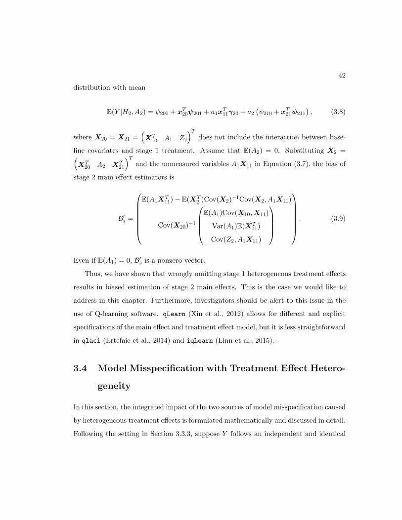
42

distribution with mean

E(Y |H2, A2) = ψ200 + xT20ψ201 + a1xT11γ20 + a2

(ψ210 + xT21ψ211

), (3.8)

where X20 = X21 =(XT

10 A1 Z2

)Tdoes not include the interaction between base-

line covariates and stage 1 treatment. Assume that E(A2) = 0. Substituting X2 =(XT

20 A2 XT21

)Tand the unmeasured variables A1X11 in Equation (3.7), the bias of

stage 2 main effect estimators is

B′s =

E(A1X

T11)− E(XT

2 )Cov(X2)−1Cov(X2, A1X11)

Cov(X20)−1

E(A1)Cov(X10,X11)

Var(A1)E(XT11)

Cov(Z2, A1X11)

. (3.9)

Even if E(A1) = 0, B′s is a nonzero vector.

Thus, we have shown that wrongly omitting stage 1 heterogeneous treatment effects

results in biased estimation of stage 2 main effects. This is the case we would like to

address in this chapter. Furthermore, investigators should be alert to this issue in the

use of Q-learning software. qLearn (Xin et al., 2012) allows for different and explicit

specifications of the main effect and treatment effect model, but it is less straightforward

in qlaci (Ertefaie et al., 2014) and iqLearn (Linn et al., 2015).

3.4 Model Misspecification with Treatment Effect Hetero-

geneity

In this section, the integrated impact of the two sources of model misspecification caused

by heterogeneous treatment effects is formulated mathematically and discussed in detail.

Following the setting in Section 3.3.3, suppose Y follows an independent and identical

43

distribution with mean

E(Y |H2, A2) = ψ200 + xT20ψ201 + a1xT11γ20 + a2

(ψ210 + xT21ψ211

),

where X20 = X21 does not include the interaction between baseline covariates and stage

1 treatment. Assume E(A1) = E(A2) = 0. In the backward induction setting, stage 1

optimization is contingent on compliance with the optimal rule at stage 2, so the true

optimal pseudo-outcome at stage 1 is

Y opt = E(Y∣∣∣H2, A2 = dopt

2

)= ψ200 + xT20ψ201 + a1x

T11γ20 −

∣∣ψ210 + xT21ψ211

∣∣ ,where dopt

2 is the optimal decision rule at stage 2 and

dopt2 (H2) = −sgn

{ψ210 + xT21ψ211

}.

For the sake of notation convention, we define X20 =(

1 XT20

)T, X21 =

(1 XT

21

)T,

ψ20 =(ψ200 ψT201

)T, and ψ21 =

(ψ210 ψT211

)T, and rewrite Y opt as

Y opt ≡ xT20ψ20 + a1xT11γ20 −

∣∣xT21ψ21

∣∣ . (3.10)

−∣∣∣XT

21ψ21

∣∣∣ represents the stage 2 optimal treatment effect, and is a non-smooth function

of ψ21. Nonregularity of stage 1 parameters due to the non-smooth function −∣∣∣XT

21ψ21

∣∣∣has been extensively studied in literature (Robins, 2004; Chakraborty et al., 2010). In

order to satisfy the regularity conditions for statistical inference, we assume

P{H2 : XT

21ψ21 = 0}

= 0. (3.11)

The estimator of Y opt is

Y opt = mina2

Q2

(x2, a2; β200, β2

)= xT20β20 −

∣∣∣xT21β21

∣∣∣ , (3.12)

44

where β20 =(β200 βT201

)Tand β21 =

(β210 βT211

)T. For large samples, β21 is a

consistent estimator of ψ21. Under assumption (3.11),∣∣∣xT21β21

∣∣∣ is also a consistent

estimator of∣∣xT21ψ21

∣∣ by the continuous mapping theorem. However,∣∣∣xT21β21

∣∣∣ is a

biased estimator of∣∣xT21ψ21

∣∣ as∣∣xT21ψ21

∣∣ 6= 0.

Normality and linearity are usually assumed for the conditional distribution of stage

2 effects on stage 1 covariates, but in stage 1 estimation, bias can still be induced

by the absolute value function∣∣xT21ψ21

∣∣. Q-learning requires the causal assumption of

no unmeasured confounders to be satisfied in order to obtain unbiased estimators of

treatment effects, i.e., the treatment model at each stage is correctly specified. Thus,

the bias discussed here does not result from misspecification of the treatment model,

but intrinsically from the misspecified linear relationship between the pseudo-outcome

and stage 1 covariates, as a result of the optimization operation. The detailed proof of

the nonlinear relationship can be found in the supplementary materials of Interactive

Model Building for Q-learning (Laber et al., 2014), and the main idea is built upon

Theorem 3.4.1.

Theorem 3.4.1. Suppose X ∼ N(µ, σ2). Then

E(|X|) =

(2σ2

π

) 12

exp

(− µ2

2σ2

)+ µ

{1− 2Φ

(−µσ

)}.

Now we derive an expression for stage 1 bias from model misspecification asso-

ciated with heterogeneous treatment effects at both stages. Rewrite Q1 (H1, A1) =

β100 +XT10β101 + a1

(β110 +XT

11β111

)≡ XT

10β10 + a1XT11β11. The values of the stage 1

parameters can be obtained as

(β10,β11) = arg minβ10,β11

E[{XT

20β20 −∣∣∣XT

21β21

∣∣∣− XT10β10 −A1X

T11β11

}2].

Let β10 and β11 be the corresponding ordinary least squares estimators. Suppose

45

X1 =(XT

10 A1XT11

)Tis the vector of predictors, X1 =

(X10 A1X11

)is the design

matrix for stage 1 estimation and is of full column rank, and Y opt is the outcome

vector with Y opti as the ith element, i = 1, . . . , n. Then the estimators of stage 1 model

parameters are

β10

β11

=(XT

1 X1

)−1XT

1 Yopt

=(XT

1 X1

)−1XT

1

(X20β20 −

∣∣∣X21β21

∣∣∣) ,and the bias of stage 1 estimation is

E(xT10β10 + a1x

T11β11

)− E(Y opt

∣∣ x1, a1)

= xT1 E{(

XT1 X1

)−1XT

1

(X20β20 −

∣∣∣X21β21

∣∣∣)}− E

(xT20ψ20 + a1x

T11γ20 −

∣∣xT21ψ21

∣∣∣∣H1, A1

)=

[xT1 E

{(XT

1 X1

)−1XT

1 B′s}− a1x

T11

]γ20 (A)

+

[E(∣∣xT21ψ21

∣∣∣∣ x1, a1

)− xT1 E

{(XT

1 X1

)−1XT

1 E(∣∣∣X21β21

∣∣∣∣∣∣H1, A1

)}], (B)

where B′s is the expression in Equation (3.9). Bias (A) is induced by the omission of

stage 1 heterogeneous treatment effects in the stage 2 main effect model, and bias (B)

is induced by the false assumption of linearity between the absolute value of stage 2

heterogeneous treatment effects and stage 1 predictors.

3.5 The Proposed Method

3.5.1 Modified Interactive Q-learning

Interactive Q-learning (Laber et al., 2014) was proposed to address the misspecified

linearity in stage 1 estimation by separately regressing stage 2 main effects on stage 1

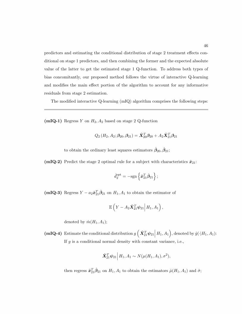
46

predictors and estimating the conditional distribution of stage 2 treatment effects con-

ditional on stage 1 predictors, and then combining the former and the expected absolute

value of the latter to get the estimated stage 1 Q-function. To address both types of

bias concomitantly, our proposed method follows the virtue of interactive Q-learning

and modifies the main effect portion of the algorithm to account for any informative

residuals from stage 2 estimation.

The modified interactive Q-learning (mIQ) algorithm comprises the following steps:

(mIQ-1) Regress Y on H2, A2 based on stage 2 Q-function

Q2 (H2, A2;β20,β21) = XT20β20 +A2X

T21β21

to obtain the ordinary least squares estimators β20, β21;

(mIQ-2) Predict the stage 2 optimal rule for a subject with characteristics x21:

dopt2 = −sgn

{xT21β21

};

(mIQ-3) Regress Y − a2xT21β21 on H1, A1 to obtain the estimator of

E(Y −A2X

T21ψ21

∣∣∣H1, A1

),

denoted by m(H1, A1);

(mIQ-4) Estimate the conditional distribution g(XT

21ψ21

∣∣∣H1, A1

), denoted by g(·|H1, A1):

If g is a conditional normal density with constant variance, i.e.,

XT21ψ21

∣∣∣H1, A1 ∼ N(µ(H1, A1), σ2),

then regress xT21β21 on H1, A1 to obtain the estimators µ(H1, A1) and σ;

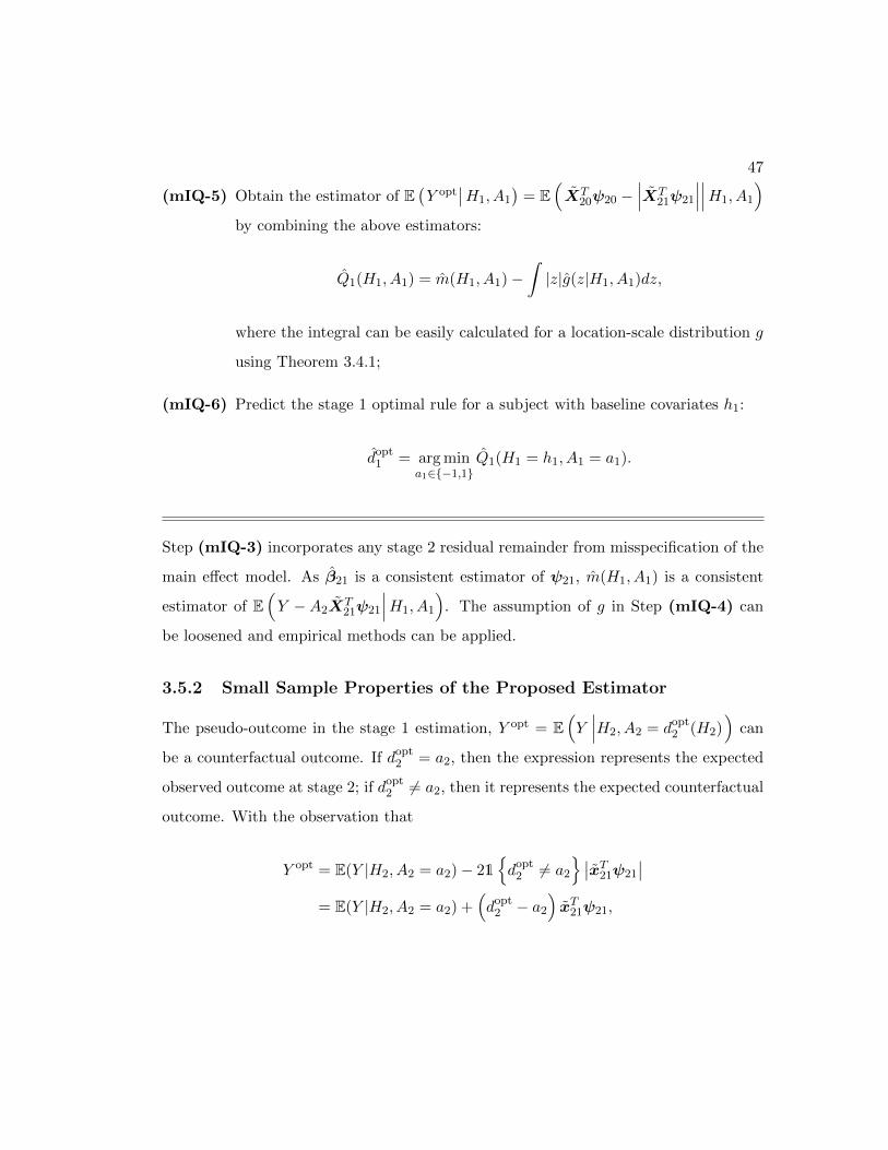
47

(mIQ-5) Obtain the estimator of E(Y opt

∣∣H1, A1

)= E

(XT

20ψ20 −∣∣∣XT

21ψ21

∣∣∣∣∣∣H1, A1

)by combining the above estimators:

Q1(H1, A1) = m(H1, A1)−∫|z|g(z|H1, A1)dz,

where the integral can be easily calculated for a location-scale distribution g

using Theorem 3.4.1;

(mIQ-6) Predict the stage 1 optimal rule for a subject with baseline covariates h1:

dopt1 = arg min

a1∈{−1,1}Q1(H1 = h1, A1 = a1).

Step (mIQ-3) incorporates any stage 2 residual remainder from misspecification of the

main effect model. As β21 is a consistent estimator of ψ21, m(H1, A1) is a consistent

estimator of E(Y −A2X

T21ψ21

∣∣∣H1, A1

). The assumption of g in Step (mIQ-4) can

be loosened and empirical methods can be applied.

3.5.2 Small Sample Properties of the Proposed Estimator

The pseudo-outcome in the stage 1 estimation, Y opt = E(Y∣∣∣H2, A2 = dopt

2 (H2))

can

be a counterfactual outcome. If dopt2 = a2, then the expression represents the expected

observed outcome at stage 2; if dopt2 6= a2, then it represents the expected counterfactual

outcome. With the observation that

Y opt = E(Y |H2, A2 = a2)− 21{dopt

2 6= a2

} ∣∣xT21ψ21

∣∣= E(Y |H2, A2 = a2) +

(dopt

2 − a2

)xT21ψ21,

48

the estimator of stage 1 Q-function, Q1(H1, A1), has a bias of

Bias(Q1

)= E

{XT

1

(X1X

T1

)−1X1

(Y −A2X

T21β21

)}− E

{Eg(∣∣∣XT

21ψ21

∣∣∣∣∣∣H1, A1

)}− E

{Y +

(dopt

2 −A2

)XT

21ψ21

∣∣∣H1, A1

}= E

{XT

1

(X1X

T1

)−1X1Y

}− E(Y |H1, A1) (3.13)

−[E{Eg(∣∣∣XT

21ψ21

∣∣∣∣∣∣H1, A1

)}− E

(∣∣∣XT21ψ21

∣∣∣∣∣∣H1, A1

)](3.14)

Therefore, unbiased estimation of stage 1 Q-function requires that (1) stage 1 model

is correctly specified so that the linearity between Y and stage 1 predictors is valid

(shown by Formula (3.13)), and (2) the assumption of normality of the underlying

distribution g is true so that the conditional distribution of stage 2 treatment effects

on stage 1 predictors is consistently estimated (shown by Formula (3.14)). Laber et al.

(2014) proposed additional nonparametric modeling of g using empirical methods, which

helps to increase the modeling flexibility of this algorithm.

3.6 Simulation

3.6.1 Preliminaries

We conduct a simulation study to show the predictive performance of the proposed

algorithm in the context of small samples. We start the discussion with a description

of the data generative mechanism. Assume a sequence of observations from a SMART

study is (Z1i, A1i, Z2i, A2i, Yi), i = 1, . . . , n, where Z1ii.i.d.∼ N(−2, 1), Z2i = Z1i + φi

and φii.i.d.∼ N(0, 4), A1i and A2i both follow an i.i.d. Rademacher distribution, so

A1i + 1

2

i.i.d.∼ Bernoulli(0.5) andA2i + 1

2

i.i.d.∼ Bernoulli(0.5). There is no embedded

tailoring variable in this design. Suppose

Yi = XT20,iψ20 + c2A2iX

T21,iψ21 + εi,

49

where εii.i.d.∼ N(0, 1) and small values of Yi are preferred. The preliminary study

considers three scenarios for the stage 2 main effects and two scenarios for the stage 2

treatment effects:

Stage 1 treatment effects Stage 2 treatment effects

XT20,iψ20 = 3− Z1i + 0.1A1i − 0.1Z2i + c1Vi XT

21,iψ21 = −6 + α1Z1i + 5A1i + α2Z2i

Homogeneous Homogeneous• Vi uncorrelated with H2i: Vi ∼ N(−1, 1) • α1 = 0, α2 = 0• Vi correlated with H2i: Vi ∼ N(2Z1iZ2i, 1)Heterogeneous Heterogeneous• Vi = Z1iA1i • α1 = −4, α2 = −0.2

Table 3.1: Specifications of stage 2 main effect and treatment effect model in the datagenerative mechanism.

For a data generative mechanism that utilizes one specification of both XT20,iψ20

and XT21,iψ21, we generate training datasets of sample size n, and a test dataset of N

subjects with potential outcomes under the four treatment regimes for each subject.

Hence, the true optimal rules, dopt1 and dopt

2 , are known for each subject in the test

dataset by minimizing the potential outcomes over all treatment regimes. The training

datasets are then used to estimate the linear models specified at each stage, and the

estimated models are used to predict the optimal rules dopt1 and dopt

2

(dopt

1

)for each

subject in the test dataset. In our framework, Z2 is defined as the set of stage 2 time-

varying covariates and tailoring variables. Note that in this setting, Z2 does not vary

with A1 in predicting dopt2 . Thus, we do not need to worry about the change in Z2 with

respect to dopt1 which in turn affects the prediction of dopt

2

(dopt

1

).

Preliminary results (Table 3.2) show that omission of stage 1 heterogeneous treat-

ment effects in stage 2 main effect model causes significant bias in stage 1 rule identifica-

tion. Omission of a variable that is uncorrelated with other stage 2 main predictors does

not cause bias, but if the omitted variable is correlated with other main predictors, then

bias is generated. Interactive Q-learning indeed does not tackle this problem and may

50

have a slightly worse performance than standard Q-learning in this scenario. Onwards,

we focus on the performance of our proposed method in the case where both stage 1 and

stage 2 treatment effects are heterogeneous, i.e., Vi = Z1iA1i and α1 = −4, α2 = −0.2.

c1 = 0 c1 = 1 c1 = 2 c1 = 3 c1 = 4

Q-learningVi ∼ N(−1, 1) 1 1 1 1 1

Vi ∼ N(2Z1iZ2i, 1) 1 1 1 0.992 0.981Vi = Z1iA1i 1 1 0.965 0.707 0.543

Interactive Q-learningVi ∼ N(−1, 1) 1 1 1 1 1

Vi ∼ N(2Z1iZ2i, 1) 1 1 0.998 0.990 0.976Vi = Z1iA1i 1 1 0.965 0.707 0.541

Table 3.2: Percentage of correctly identified stage 1 optimal rules when stage 2 treatmenteffects are homogeneous across subjects (α1 = α2 = 0), prediction using standard Q-learning and interactive Q-learning, based on a set of test data (N = 10000) and 100simulations of training data (n = 250).

3.6.2 Results

We compare the proposed method (mIQ) with standard Q-learning (sQ), modified Q-

learning (mQ; Huang et al. (2015)), and interactive Q-learning (IQ; Laber et al. (2014)).

c1 c2 sQ mQ IQ mIQ

0.01.0 0.963 0.963 0.969 0.9692.0 0.969 0.970 0.976 0.9763.0 0.969 0.969 0.973 0.973

2.01.0 0.869 0.965 0.910 0.9852.0 0.900 0.964 0.947 0.9813.0 0.921 0.966 0.963 0.979

4.01.0 0.893 0.972 0.892 0.9862.0 0.871 0.966 0.910 0.9853.0 0.883 0.963 0.934 0.981

Table 3.3: Percentage of correctly identified stage 1 optimal rules when stage 2 treatmenteffects are heterogeneous across subjects (α1 = −4, α2 = −0.2), based on a set of testdata (N = 10000) and 100 simulations of training data (n = 250).

51

Table 3.3 summarizes the probabilities of correctly identifying stage 1 optimal rules

based on the four methods considered, and mIQ has the highest accuracy across all

scenarios. The results show that the modified interactive Q-learning algorithm corrects

for potential bias generated from both stage 1 and stage 2 heterogeneous treatment effects.

Figure 3.2: Probability of correctly identifying stage 1 optimal rules as a function of c2

for c1 = 0, 2, 4.

Figure 3.2 plots the trend with varied c2 at finer intervals for the three values of

c1. If stage 1 treatment effects are homogeneous (c1 = 0), then the four methods work

similarly, and modified interactive Q-learning performs exactly the same as interactive

Q-learning. If stage 1 treatment effects are highly heterogeneous (c1 = 4), then modified

interactive outperforms all other methods, and there is a substantial difference in the

probability of correctly identifying stage 1 optimal rules between modified Q-learning

and modified interactive Q-learning. It further stresses the importance of building

interactive models into modified Q-learning.

52

3.7 Data Analysis

We use the M-bridge data (n = 591) to illustrate the application of the proposed method

on SMARTs with embedded tailoring. Figure 3.1 shows the design of M-bridge for this

analysis. Our aim is to identify the personalized optimal DTR for each subject in the

dataset, which minimizes binge drinking (primary outcome, 490 subjects with complete

data on the maximum number of drinks within a 24-hour period at baseline and follow-

up), and negative drinking-related consequences (secondary outcome, 496 subjects with

complete data on the total number of drinking-related consequences in the past 30

days at baseline and follow-up). We perform the data analysis separately for these two

outcomes.

Stage 2 model uses as covariates baseline characteristics, including gender, race,

intention to pledge Greek, indicator whether parent has a significant drinking problem,

pre-college drinking norms and intention for college drinking, and pre-college drinking

habits, and the interaction between stage 2 intervention and baseline characteristics.

Stage 1 model uses as covariates baseline characteristics and their interaction with

stage 1 intervention. A summary of the covariates and outcomes used in the model is

presented in Table 3.4.

Table 3.4: Summary statistics of subject characteristics by initial randomization (stage1 intervention). Discrete variables are summarized by counts; continuous variables aresummarized by mean (SD).

Early Intervention Late Intervention Overall

(n1 = 295) (n2 = 296) (n = 591)

Demographics

Gender

Male 115 104 219

Female 180 192 372

Continued on next page

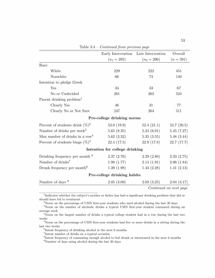
53

Table 3.4 – Continued from previous page


(n1 = 295) (n2 = 296) (n = 591)

Race

White 229 222 451

Nonwhite 66 74 140

Intention to pledge Greek

Yes 34 33 67

No or Undecided 261 263 524

Parent drinking problem1

Clearly Yes 46 31 77

Clearly No or Not Sure 247 264 511

Pre-college drinking norms

Percent of students drink (%)2 53.0 (19.9) 52.4 (21.1) 52.7 (20.5)

Number of drinks per week3 5.65 (8.35) 5.24 (6.01) 5.45 (7.27)

Max number of drinks in a row4 5.62 (3.32) 5.35 (3.55) 5.48 (3.44)

Percent of students binge (%)5 22.4 (17.5) 22.9 (17.8) 22.7 (17.7)

Intention for college drinking

Drinking frequency per month 6 2.37 (2.70) 2.29 (2.80) 2.33 (2.75)

Number of drinks7 1.98 (1.77) 2.14 (1.91) 2.06 (1.84)

Drunk frequency per month8 1.39 (1.98) 1.43 (2.28) 1.41 (2.13)

Pre-college drinking habits

Number of days 9 2.05 (3.09) 2.03 (3.25) 2.04 (3.17)

Continued on next page

1Indicator whether the subject’s mother or father has had a significant drinking problem that did orshould have led to treatment

2Norm on the percentage of UMN first-year students who used alcohol during the last 30 days3Norm on the number of alcoholic drinks a typical UMN first-year student consumed during an

average week4Norm on the largest number of drinks a typical college student had in a row during the last two

weeks5Norm on the percentage of UMN first-year students had five or more drinks in a sitting during the

last two weeks6Intent frequency of drinking alcohol in the next 6 months7Intent number of drinks on a typical occasion8Intent frequency of consuming enough alcohol to feel drunk or intoxicated in the next 6 months9Number of days using alcohol during the last 30 days

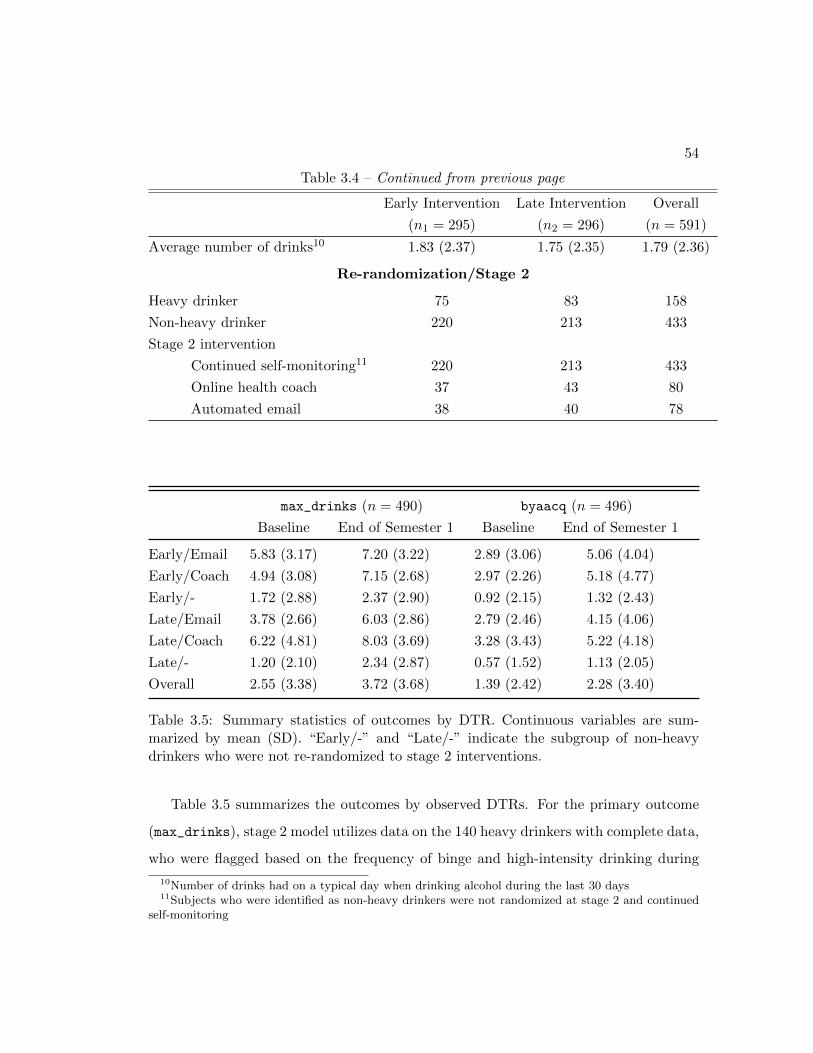
54

Table 3.4 – Continued from previous page


(n1 = 295) (n2 = 296) (n = 591)

Average number of drinks10 1.83 (2.37) 1.75 (2.35) 1.79 (2.36)

Re-randomization/Stage 2

Heavy drinker 75 83 158

Non-heavy drinker 220 213 433

Stage 2 intervention

Continued self-monitoring11 220 213 433

Online health coach 37 43 80

Automated email 38 40 78

max_drinks (n = 490) byaacq (n = 496)

Baseline End of Semester 1 Baseline End of Semester 1

Early/Email 5.83 (3.17) 7.20 (3.22) 2.89 (3.06) 5.06 (4.04)

Early/Coach 4.94 (3.08) 7.15 (2.68) 2.97 (2.26) 5.18 (4.77)

Early/- 1.72 (2.88) 2.37 (2.90) 0.92 (2.15) 1.32 (2.43)

Late/Email 3.78 (2.66) 6.03 (2.86) 2.79 (2.46) 4.15 (4.06)

Late/Coach 6.22 (4.81) 8.03 (3.69) 3.28 (3.43) 5.22 (4.18)

Late/- 1.20 (2.10) 2.34 (2.87) 0.57 (1.52) 1.13 (2.05)

Overall 2.55 (3.38) 3.72 (3.68) 1.39 (2.42) 2.28 (3.40)

Table 3.5: Summary statistics of outcomes by DTR. Continuous variables are sum-marized by mean (SD). “Early/-” and “Late/-” indicate the subgroup of non-heavydrinkers who were not re-randomized to stage 2 interventions.

Table 3.5 summarizes the outcomes by observed DTRs. For the primary outcome

(max_drinks), stage 2 model utilizes data on the 140 heavy drinkers with complete data,

who were flagged based on the frequency of binge and high-intensity drinking during

10Number of drinks had on a typical day when drinking alcohol during the last 30 days11Subjects who were identified as non-heavy drinkers were not randomized at stage 2 and continued

self-monitoring

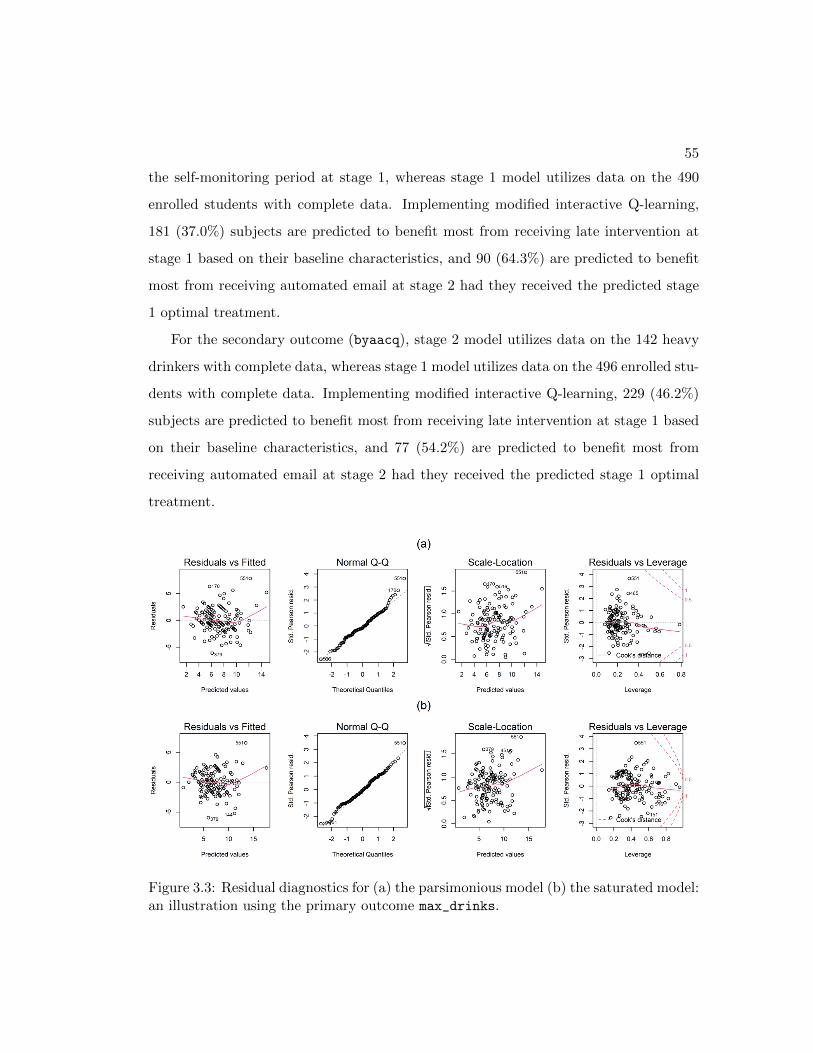
55

the self-monitoring period at stage 1, whereas stage 1 model utilizes data on the 490

enrolled students with complete data. Implementing modified interactive Q-learning,

181 (37.0%) subjects are predicted to benefit most from receiving late intervention at

stage 1 based on their baseline characteristics, and 90 (64.3%) are predicted to benefit

most from receiving automated email at stage 2 had they received the predicted stage

1 optimal treatment.

For the secondary outcome (byaacq), stage 2 model utilizes data on the 142 heavy

drinkers with complete data, whereas stage 1 model utilizes data on the 496 enrolled stu-

dents with complete data. Implementing modified interactive Q-learning, 229 (46.2%)

subjects are predicted to benefit most from receiving late intervention at stage 1 based

on their baseline characteristics, and 77 (54.2%) are predicted to benefit most from

receiving automated email at stage 2 had they received the predicted stage 1 optimal

treatment.

Figure 3.3: Residual diagnostics for (a) the parsimonious model (b) the saturated model:an illustration using the primary outcome max_drinks.

56

The proposed method requires that any missingness in the outcome measurements

is not informative. M-bridge might not be a perfect example of informative residuals,

because the interaction between A1 and Z1 does not have a significantly impact on

the outcome. Figure 3.3 shows that, for the primary outcome, residual diagnostics of

the parsimonious model do not differ much from those of the saturated model. How-

ever, modified interactive Q-learning still helps as the huge amount of baseline covari-

ates might cause the problem of overfitting. Nevertheless, we anticipate that modified

interactive Q-learning performs similarly as interactive Q-learning in this case. The

comparison is shown in the supplementary materials.

3.8 Discussion

This chapter attempts to understand the bias caused by misspecification of the main

effect model in the implementation of Q-learning, specifically, omitting an unmeasured

variable, and confirms the existence of bias when the unmeasured variable is correlated

with the observed predictors (especially stage 1 treatment). As stage 1 heterogeneous

treatment effects are usually neglected in the stage 2 main effect model and might be

a significant predictor, we then modify the Q-learning algorithm to account for the

unexplained residuals. This modification is then built into the interactive Q-learning,

which corrects the bias generated by stage 2 heterogeneous treatment effects and the

optimization operation, to improve the overall performance where both stage 1 and 2

treatment effects are heterogeneous. The proposed method and the simulation results

assume that the two randomization arms at each stage are equally assigned. If the

randomization scheme has an unbalanced allocation ratio, then the estimators of stage

2 treatment effects would be biased in the presence of an unmeasured variable. Future

work and exploration of Q-learning in this context would be merited.

Chapter 4

A Generalization to Dichotomous

Outcomes

4.1 Background

Clinical investigators are commonly interested in dichotomous endpoints as the outcome

can be easily differentiated across subjects, especially when there is a gold standard

cut-off point with a clear justification. To optimize DTRs for dichotomous outcomes,

one common method is Q-learning with logistic or probit regression. This chapter

aims to address the informative residuals due to misspecification of late-stage main

effect model for dichotomous outcomes. Methods that posit more flexibility in modeling

Q-functions include generalized additive model (Moodie et al., 2014), which allows a

nonlinear relationship between outcome and predictors, and Bayesian machine learning

(Murray et al., 2018), which obviates the nonregularity problem in Q-learning and

utilizes a probit Bayesian additive regression trees model for the dichotomous outcomes.

Despite the fact that these methods perform well in many circumstances, they are not

developed for the purpose of dealing with informative residuals. For Q-learning with

linear regression, a modification with Murphy’s regret function (Huang et al., 2015) was

57

58

proposed to correct for the informative residuals. However, a difficulty arises if modified

Q-learning is used for dichotomous outcomes, as the probability of a success is linked

to the linear combination of predictors using a non-identity function.

One solution to this problem would be imposing monotonicity of preferences to early-

stage pseudo-outcomes. If a subject was observed to receive an optimal treatment, then

the corresponding pseudo-outcome would be the observed outcome. If a subject was

observed to receive a suboptimal treatment and responded with the desirable outcome,

then they must have responded, had they received the optimal treatment. However,

there is no restriction that we could impose on potential pseudo-outcomes for subjects

who received the suboptimal treatment and responded with the undesirable outcome.

These subjects could possibly respond with desirable or undesirable outcomes had they

received the optimal treatment. Therefore, this approach results in a loss of information.

We present Q-learning with probit regression and the proposed modification in Sec-

tion 4.2. A simulation study is performed in Section 4.3 to investigate the potential

improvement of the modification. The data example in Section 3.2.1 with a different

set of outcomes is used to illustrate the methods, and the results are summarized in

Section 4.4. Moreover, probit regression is equivalent to a latent variable model where

the underlying continuous variable is modeled explicitly. In Section 4.5, we discuss the

feasibility of using latent variable modeling to correctly estimate the underlying continu-

ous variable, and propose a novel algorithm which samples surrogates from a truncated

normal distribution as estimates of the latent variable and adds back the Murphy’s

regret function to generate early-stage pseudo-outcomes.

4.2 Methods

Suppose that the data collected from a SMART are represented by a sequence of inde-

pendently and identically distributed random variables (Z1, A1, Z2, A2, Y ), where Z1 is

the set of baseline covariates and moderators measured prior to stage 1 randomization,

59

Z2 is the set of time-varying covariates and potential tailoring variables measured be-

tween stage 1 and stage 2 randomizations, Ak ∈ Ak, k = 1, 2, is the treatment at stage

k, with Ak being the set of all possible treatments, and Y ∈ (0, 1) is the dichotomous

outcome measured after treatment stages, with Y = 0 preferred.

In the M-bridge study, the investigators are primarily interested in preventing binge

and high-intensity drinking, so whether a student had binge drinking, i.e., the frequency

of binge drinking was greater than 0, would be an outcome of great interest. We hypoth-

esize a scenario where the actual frequency of binge drinking for each college student is

hidden in the data cleaning process, and we only have the information whether the fre-

quency of binge drinking is greater than 0. A value of 0 is preferred for the indicator of

binge drinking. The secondary outcome considered by the investigators is health services

utilization, which is a dichotomous measure of whether students used any health services

over the past three months, including through a healthcare clinic, individual counseling,

group therapy, support groups, self-help resources, or other services/resources. A value

of 1 is preferred for health services utilization.

4.2.1 Q-learning with Probit Regression

One commonly used method to optimize DTRs for binary outcomes in the literature

is Q-learning with logistic regression or probit regression. With the probit link, an

equivalent formulation is to assume that there is a latent variable that is linearly related

to covariates with an error term following a standard normal distribution, and we only

observe the indicator for whether the latent variable is greater than a certain threshold.

The alternative formulation will be discussed in detail in Section 4.5.

Consider the model for Q2(H2, A2) = E(Y |H2, A2) = P(Y = 1|H2, A2):

Q2(H2i, A2i;β20,β21) = Φ(xT20,iβ20 + a2x

T21,iβ21

), (4.1)

where Φ is the cumulative distribution function of a standard normal random variable.

60

As Φ is a monotonically increasing function, the stage 2 optimal rule is

dopt2i = arg min

a2∈{−1,1}Φ(xT20,iβ20 + a2x

T21,iβ21

)= −sgn

{xT21,iβ21

}.

The pseudo-outcome at stage 1, conditional on stage 2 optimization, is

Y1i = mina2∈{−1,1}

Φ−1Q2(H2i, A2i = a2) = xT20,iβ20 −∣∣∣xT21,iβ21

∣∣∣ . (4.2)

Consider Q1(Hi1, A1i;β10,β11) = xT10,iβ10 +a1xT11,iβ11. Stage 1 least squares estimators

are obtained by

(β10, β11

)= arg min

β10,β11

1

n

n∑i=1

{Y1i −Q1(Hi1, A1i;β10,β11)

}2.

The stage 1 optimal rule is estimated as

dopt1i = arg min

a1∈{−1,1}Q1

(Hi1, A1i; β10, β11

)= −sgn

{xT11,iβ11

}.

Logit link is sometimes preferred in stage 2 estimation to analyze real data, as it leads

to the estimation of a commonly used association measure, odds ratio, which is easily

interpretable by clinical investigators. Nevertheless, both link functions produce similar

results.

4.2.2 The Proposed Modification

If the main effect model of the stage 2 Q-function in Equation (4.1) is misspecified, i.e.,

an important predictor is omitted, it is difficult to correct for any informative residual

remaining due to the presence of the non-identity link. It is, therefore, tempting to

impose some restrictions directly on stage 1 pseudo-outcome Y1 so that the imputed

distribution over Y1 is closer to reality. Our proposed modification follows the concept

of Murphy’s regret function. At stage 2, if a subject is observed to receive the optimal

61

treatment, then the stage 1 pseudo-outcome would be the same as the observed out-

come. On the other hand, if a subject receives the suboptimal treatment, we are not

able to simply add back Murphy’s regret function to obtain the counterfactual outcome

under the optimal treatment. Instead, we impose monotonicity of preferences, i.e., the

treatment which yields a more desirable potential outcome is always preferred. Thus,

the treatment associated with the most desirable potential outcome is optimal. Specif-

ically, if a subject receives the suboptimal treatment and responds with the desirable

outcome Y = 0, then they must have responded with Y = 0 had they received the

optimal treatment. If a subject receives the suboptimal treatment and responds with

the undesirable outcome Y = 1, then we cannot make any correction to stage 1 pseudo-

outcome as it is not guaranteed that the subject would respond desirably enough to

reach Y = 0 counterfactually. The stage 1 pseudo-outcome in this case should still be

drawn from the model in Equation (4.1). If the estimated optimal probability of an

event, mina2∈{−1,1}

P(Y = 1|H2, A2 = a2), is greater than 0.5, then we assign the stage 1

pseudo-outcome as 1; otherwise we assign the stage 1 pseudo-outcome as 0. Thus, the

modified pseudo-outcome at stage 1, conditional on stage 2 optimization, is

Y m1i = 1

{dopt

2i = A2i

}Yi

+ 1{dopt

2i 6= A2i

}[1 {Yi = 0}Yi + 1 {Yi = 1}1

{Φ(Y1i

)> 0.5

}]= 1

{dopt

2i = A2i

}Yi + 1

{dopt

2i 6= A2i

}1 {Yi = 1}1

{Φ(Y1i

)> 0.5

}. (4.3)

where Y1i is defined in Equation (4.2) and Φ(Y1i

)= min

a2∈{−1,1}Q2

(H2i, A2i = a2; β20, β21

).

Different from Q-learning with probit regression, where we obtain stage 1 estima-

tors directly using least squares estimation, stage 1 estimators in the modified algo-

rithm are again obtained by a probit regression. Consider Q1(Hi1, A1i;β10,β11) =

62

Φ(xT10,iβ10 + a1x

T11,iβ11

). The stage 1 optimal rule is estimated as

dopt1i = arg min

a1∈{−1,1}Φ(xT10,iβ10 + a1x

T11,iβ11

)= −sgn

{xT11,iβ11

}.

The definition of Y m1i in Equation (4.3) has a piece of information missing: if a subject

receives a suboptimal treatment and responds with the undesirable outcome Y = 1,

though we are not able to make any assumption on stage 1 pseudo-outcome, the un-

derlying continuous variable should have at most the same value had they received the

optimal treatment. Since the proposed modification does not utilize all the information,

its performance is expected to be compromised. However, the proposed approach has

some potential advantages to release the reliance of Q-learning with probit regression

on the correct specification of stage 2 Q-function.

4.3 Simulation Study

We conduct a simulation study to assess the performance of the proposed modification.

Assume a sequence of data collected from a two-stage SMART study is

(Z1i, A1i, Z2i, A2i, Yi), i = 1, . . . , n,

where Z1ii.i.d.∼ N(−2, 1), Z2i = Z1i + φi and φi

i.i.d.∼ N(0, 1),A1i + 1

2

i.i.d.∼ Bernoulli(0.5)

andA2i + 1

2

i.i.d.∼ Bernoulli(0.5). There is no embedded tailoring variable in this design.

Suppose

Yi = 1{3− Z1i + 0.1A1i − 0.1Z2i + γZ1iA1i

+A2i (−9− 6Z1i + 7.5A1i − 0.3Z2i) + εi > 10},

where εii.i.d.∼ N(0, σ2). Suppose Yi = 0 is preferred.

A test dataset of N subjects is generated with potential outcomes under the four

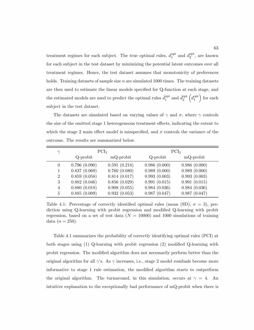
63

treatment regimes for each subject. The true optimal rules, dopt1 and dopt

2 , are known

for each subject in the test dataset by minimizing the potential latent outcomes over all

treatment regimes. Hence, the test dataset assumes that monotonicity of preferences

holds. Training datasets of sample size n are simulated 1000 times. The training datasets

are then used to estimate the linear models specified for Q-function at each stage, and

the estimated models are used to predict the optimal rules dopt1 and dopt

2

(dopt

1

)for each

subject in the test dataset.

The datasets are simulated based on varying values of γ and σ, where γ controls

the size of the omitted stage 1 heterogeneous treatment effects, indicating the extent to

which the stage 2 main effect model is misspecified, and σ controls the variance of the

outcome. The results are summarized below.

γ PCI1 PCI2

Q-probit mQ-probit Q-probit mQ-probit

0 0.796 (0.090) 0.591 (0.218) 0.986 (0.000) 0.986 (0.000)1 0.837 (0.069) 0.760 (0.080) 0.989 (0.000) 0.989 (0.000)2 0.859 (0.058) 0.814 (0.017) 0.993 (0.003) 0.993 (0.003)3 0.882 (0.046) 0.856 (0.029) 0.991 (0.015) 0.991 (0.015)4 0.880 (0.018) 0.908 (0.055) 0.984 (0.036) 0.984 (0.036)5 0.885 (0.009) 0.932 (0.053) 0.987 (0.047) 0.987 (0.047)

Table 4.1: Percentage of correctly identified optimal rules (mean (SD); σ = 3), pre-diction using Q-learning with probit regression and modified Q-learning with probitregression, based on a set of test data (N = 10000) and 1000 simulations of trainingdata (n = 250).

Table 4.1 summarizes the probability of correctly identifying optimal rules (PCI) at

both stages using (1) Q-learning with probit regression (2) modified Q-learning with

probit regression. The modified algorithm does not necessarily perform better than the

original algorithm for all γ’s. As γ increases, i.e., stage 2 model residuals become more

informative to stage 1 rule estimation, the modified algorithm starts to outperform

the original algorithm. The turnaround, in this simulation, occurs at γ = 4. An

intuitive explanation to the exceptionally bad performance of mQ-probit when there is

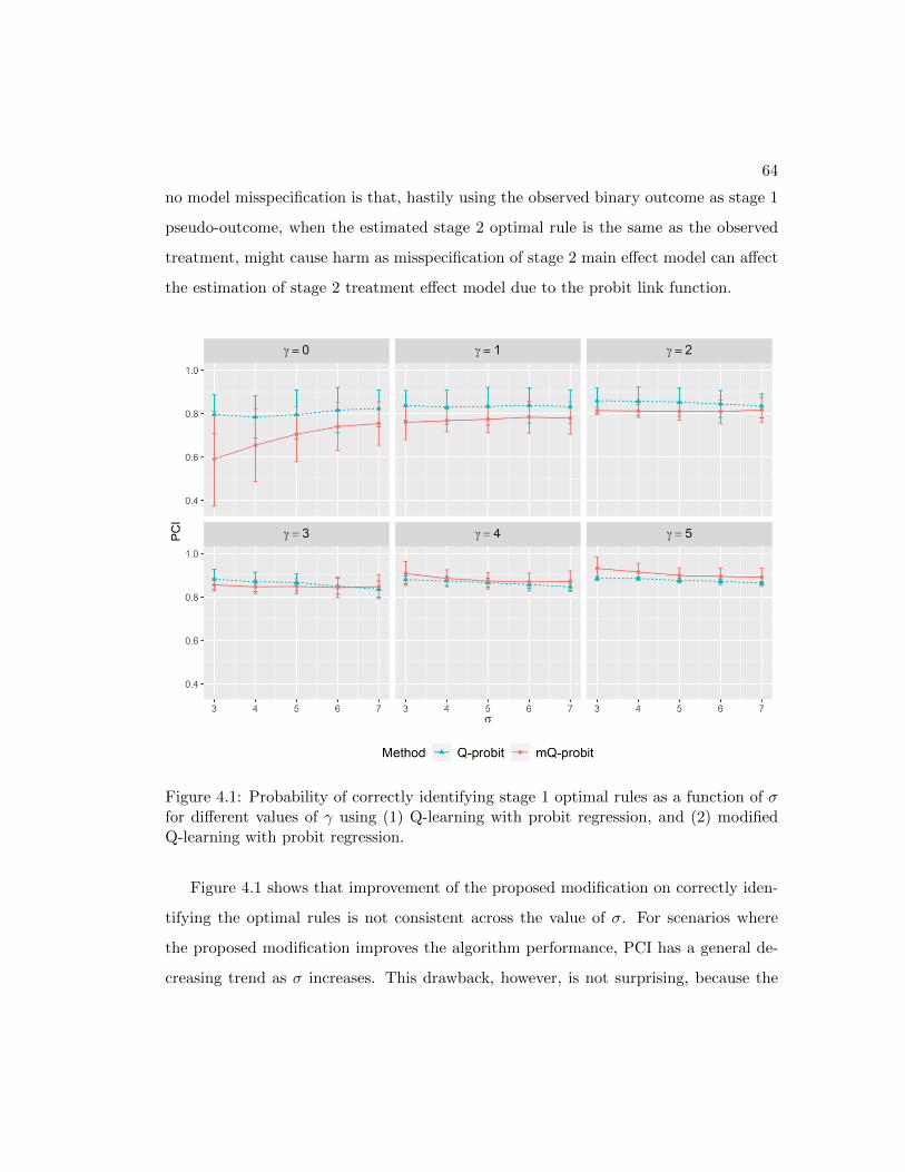
64

no model misspecification is that, hastily using the observed binary outcome as stage 1

pseudo-outcome, when the estimated stage 2 optimal rule is the same as the observed

treatment, might cause harm as misspecification of stage 2 main effect model can affect

the estimation of stage 2 treatment effect model due to the probit link function.

Figure 4.1: Probability of correctly identifying stage 1 optimal rules as a function of σfor different values of γ using (1) Q-learning with probit regression, and (2) modifiedQ-learning with probit regression.

Figure 4.1 shows that improvement of the proposed modification on correctly iden-

tifying the optimal rules is not consistent across the value of σ. For scenarios where

the proposed modification improves the algorithm performance, PCI has a general de-

creasing trend as σ increases. This drawback, however, is not surprising, because the

65

uncertainty of classifying the outcome as desirable or undesirable increases as the un-

derlying latent variable is largely dispersed.

4.4 Data Analysis

We use the M-bridge data (n = 591) to illustrate the application of modified Q-learning

with probit regression on SMARTs with embedded tailoring. We follow the design

illustrated in Section 3.2.1 for this analysis, but analyze a different set of outcomes.

Our aim is to identify the personalized optimal DTR for each subject in the dataset,

which minimizes binge drinking (primary outcome, 495 subjects with complete data on

the frequency of binge drinking during the last 30 days at baseline and follow-up), or

maximizes health services utilization (secondary outcome, 493 subjects with complete

data on if the subject used any health resources or services indicated in the questionnaire

in the last 3 months at baseline and follow-up). We perform data analysis separately

for these two outcomes.

ind_binge (%) hs_util (%)

n Baseline Semester 1 n Baseline Semester 1

Early/Email 36 66.7 88.9 36 72.2 52.8

Early/Coach 33 51.5 93.9 33 60.6 48.5

Early/- 179 16.8 24.6 178 71.3 52.8

Late/Email 33 57.6 75.8 33 81.8 54.5

Late/Coach 40 62.5 92.5 40 70.0 55.0

Late/- 174 12.6 25.9 173 72.8 56.6

Overall 495 27.7 43.2 493 71.8 54.2

Table 4.2: Summary statistics of outcomes by DTR: the percentage of subjects whohad binge drinking, and the percentage of subjects who did not utilize health services.Higher percentage is undesirable. “Early/-” and “Late/-” indicate the subgroup of non-heavy drinkers who were not re-randomized to stage 2 interventions, and n denotes thesample size in each DTR.

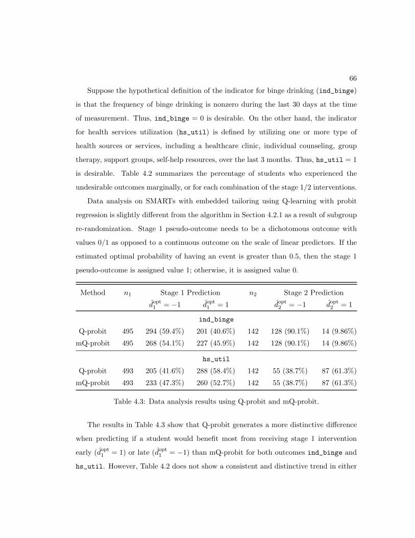
66

Suppose the hypothetical definition of the indicator for binge drinking (ind_binge)

is that the frequency of binge drinking is nonzero during the last 30 days at the time

of measurement. Thus, ind_binge = 0 is desirable. On the other hand, the indicator

for health services utilization (hs_util) is defined by utilizing one or more type of

health sources or services, including a healthcare clinic, individual counseling, group

therapy, support groups, self-help resources, over the last 3 months. Thus, hs_util = 1

is desirable. Table 4.2 summarizes the percentage of students who experienced the

undesirable outcomes marginally, or for each combination of the stage 1/2 interventions.

Data analysis on SMARTs with embedded tailoring using Q-learning with probit

regression is slightly different from the algorithm in Section 4.2.1 as a result of subgroup

re-randomization. Stage 1 pseudo-outcome needs to be a dichotomous outcome with

values 0/1 as opposed to a continuous outcome on the scale of linear predictors. If the

estimated optimal probability of having an event is greater than 0.5, then the stage 1

pseudo-outcome is assigned value 1; otherwise, it is assigned value 0.

Method n1 Stage 1 Prediction n2 Stage 2 Prediction

dopt1 = −1 dopt

1 = 1 dopt2 = −1 dopt

2 = 1

ind_binge

Q-probit 495 294 (59.4%) 201 (40.6%) 142 128 (90.1%) 14 (9.86%)

mQ-probit 495 268 (54.1%) 227 (45.9%) 142 128 (90.1%) 14 (9.86%)

hs_util

Q-probit 493 205 (41.6%) 288 (58.4%) 142 55 (38.7%) 87 (61.3%)

mQ-probit 493 233 (47.3%) 260 (52.7%) 142 55 (38.7%) 87 (61.3%)

Table 4.3: Data analysis results using Q-probit and mQ-probit.

The results in Table 4.3 show that Q-probit generates a more distinctive difference

when predicting if a student would benefit most from receiving stage 1 intervention

early (dopt1 = 1) or late (dopt

1 = −1) than mQ-probit for both outcomes ind_binge and

hs_util. However, Table 4.2 does not show a consistent and distinctive trend in either

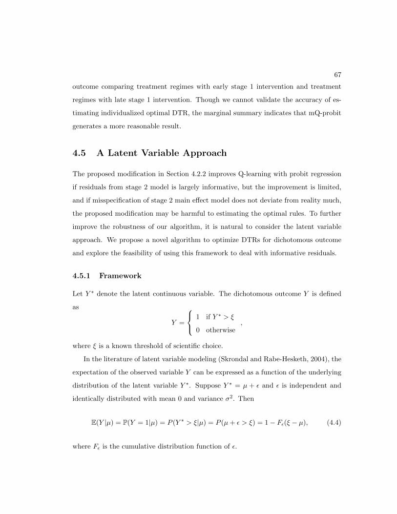
67

outcome comparing treatment regimes with early stage 1 intervention and treatment

regimes with late stage 1 intervention. Though we cannot validate the accuracy of es-

timating individualized optimal DTR, the marginal summary indicates that mQ-probit

generates a more reasonable result.

4.5 A Latent Variable Approach

The proposed modification in Section 4.2.2 improves Q-learning with probit regression

if residuals from stage 2 model is largely informative, but the improvement is limited,

and if misspecification of stage 2 main effect model does not deviate from reality much,

the proposed modification may be harmful to estimating the optimal rules. To further

improve the robustness of our algorithm, it is natural to consider the latent variable

approach. We propose a novel algorithm to optimize DTRs for dichotomous outcome

and explore the feasibility of using this framework to deal with informative residuals.

4.5.1 Framework

Let Y ∗ denote the latent continuous variable. The dichotomous outcome Y is defined

as

Y =

1 if Y ∗ > ξ

0 otherwise,

where ξ is a known threshold of scientific choice.

In the literature of latent variable modeling (Skrondal and Rabe-Hesketh, 2004), the

expectation of the observed variable Y can be expressed as a function of the underlying

distribution of the latent variable Y ∗. Suppose Y ∗ = µ + ε and ε is independent and

identically distributed with mean 0 and variance σ2. Then

E(Y |µ) = P(Y = 1|µ) = P (Y ∗ > ξ|µ) = P (µ+ ε > ξ) = 1− Fε(ξ − µ), (4.4)

where Fε is the cumulative distribution function of ε.

68

4.5.2 The Proposed Algorithm

Suppose µi = xT20,iβ20+a2xT21,iβ21. Following the formulation in Section 4.5.1, we derive

the log-likelihood of model parameters:

` (β20,β21, σ |{yi}ni=1, {y∗i }ni=1 ) = −n log σ − 1

2σ2

n∑i=1

(y∗i − xT20,iβ20 − a2x

T21,iβ21

)2.

(4.5)

Now we propose a novel algorithm called modified latent Q-learning (mLQ) to op-

timize DTRs for dichotomous outcomes. Here is a brief outline of the proposed algo-

rithm. First, we utilize an Expectation-Maximization (EM) algorithm to estimate the

stage 2 model parameters θ = (β20,β21, σ). Using an idea adapted from Liu and Zhang

(2018), a surrogate of Y ∗ is drawn from the conditional distribution f(y∗|y) so that the

surrogate variable follows a distribution of∑y

f(y∗|y)f(y). Note that the marginal dis-

tribution f(y) is observed, but the conditional distribution f(y∗|y) can be misspecified.

We then use the surrogate variable and Murphy’s regret function to construct stage 1

pseudo-outcomes.

The detailed steps are as follows:

Stage 2 estimation: the EM algorithm

(mLQ-1) Initialize θ(v) for v = 0;

(mLQ-2) E-step: Take the expectation of ` (θ |{yi}ni=1, {y∗i }ni=1 ) over the conditional

distribution f(Y ∗|Y ) characterized by θ(v) to obtain

Q(θ,θ(v); {yi}ni=1

)=− n log σ − 1

2σ2

n∑i=1

Eθ(v)

(y∗2i∣∣ yi)

+1

σ2

n∑i=1

µiEθ(v) (y∗i | yi)−1

2σ2

n∑i=1

µ2i , (4.6)

69

where

Eθ(v) (y∗i | yi) = µ(v)i +

(2yi − 1)σ(v)2φ(µ

(v)i , σ(v)2; ξ

)yi

{1− Φ

(µ

(v)i , σ(v)2; ξ

)}+ (1− yi)Φ

(µ

(v)i , σ(v)2; ξ

) ,Eθ(v)

(y∗2i∣∣ yi) = µ

(v)2i + σ(v)2 +

(2yi − 1)(µ(v)i + ξ)σ(v)2φ

(µ

(v)i , σ(v)2; ξ

)yi

{1− Φ

(µ

(v)i , σ(v)2; ξ

)}+ (1− yi)Φ

(µ

(v)i , σ(v)2; ξ

) ,µ

(v)i = xT20,iβ

(v)20 + a2x

T21,iβ

(v)21 ,

and φ(µ, σ2) and Φ(µ, σ2) denote the probability density function and cu-

mulative distribution function of N(µ, σ2) respectively;

(mLQ-3) M-step: Let x2i =(xT20,i a2x

T21,i

)T. Maximize Q

(θ,θ(v); {yi}ni=1

)to derive

θ(v+1) asβ(v+1)20

β(v+1)21

=

{n∑i=1

x2ixT2i

}−1{ n∑i=1

x2iEθ(v) (y∗i | yi)

},

σ(v+1) =

√√√√ 1

n

{n∑i=1

Eθ(v)

(y∗2i∣∣ yi)− 2

n∑i=1

µiEθ(v) (y∗i | yi) +n∑i=1

µ2i

};

(mLQ-4) Iterate steps 2 and 3 until convergence, where the difference in log-likelihood

is negligible;

(mLQ-5) The stage 2 optimal rule for the ith subject is estimated as

dopt2i = −sgn

{xT21,iβ21

}.

Stage 1 estimation: the linear model

(mLQ-6) Sample surrogate variables: Sample a surrogate of Y ∗i , denoted by si, for

70

each individual from a truncated normal distribution conditional on yi,

f(y∗i |yi) = yiTN(µi, σ2, ξ,∞) + (1− yi)TN(µi, σ

2,−∞, ξ),

where µi = xT20,iβ20 + a2xT21,iβ21;

(mLQ-7) Construct stage 1 pseudo-latent outcomes:

Y ∗1i = si − 21{a2i 6= dopt

2i

} ∣∣∣xT21,iβ21

∣∣∣ ; (4.7)

(mLQ-8) Obtain the least squares estimators β10 and β11 through a linear regression

E(Y ∗1i

∣∣∣H1i, A1i

)= xT10,iβ10 + a1x

T11,iβ11;

(mLQ-9) The stage 1 optimal rule for the ith subject is estimated as

dopt1i = −sgn

{xT11,iβ11

}.

The EM algorithm is equivalent to probit regression in the prediction of stage 2 optimal

rules, but yields model estimates associated with the expectation of the latent variable.

The variance, or the standard error of the estimators can be obtained using Bootstrap.

4.5.3 Simulation Study Revisited

Following the simulation setting in Section 4.3, we add the performance of the proposed

mLQ. Figure 4.2 shows that mLQ has a consistent and moderately decent performance

across all γ’s. When a reasonably small amount of model misspecification is present,

specifically, for γ = 1, 2, 3, mLQ outperforms Q-probit and mQ-probit. However, when

a sizable amount of model misspecification is present (γ ≥ 4), mLQ starts to generate

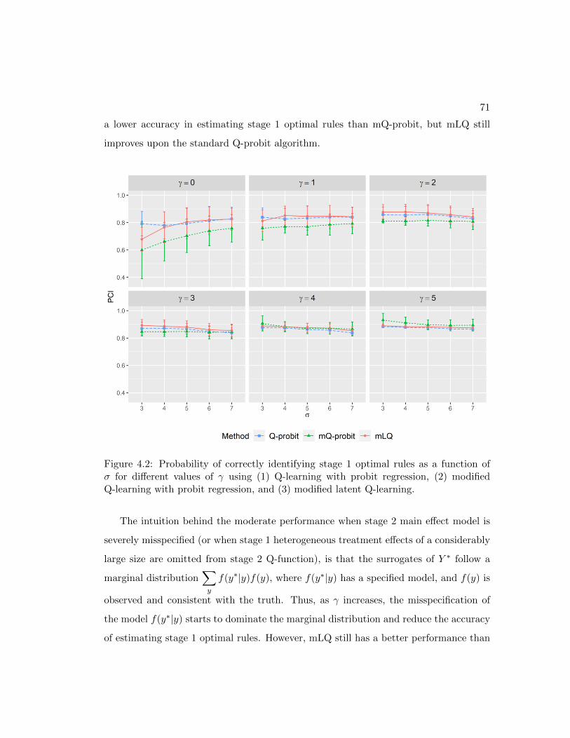
71

a lower accuracy in estimating stage 1 optimal rules than mQ-probit, but mLQ still

improves upon the standard Q-probit algorithm.

Figure 4.2: Probability of correctly identifying stage 1 optimal rules as a function ofσ for different values of γ using (1) Q-learning with probit regression, (2) modifiedQ-learning with probit regression, and (3) modified latent Q-learning.

The intuition behind the moderate performance when stage 2 main effect model is

severely misspecified (or when stage 1 heterogeneous treatment effects of a considerably

large size are omitted from stage 2 Q-function), is that the surrogates of Y ∗ follow a

marginal distribution∑y

f(y∗|y)f(y), where f(y∗|y) has a specified model, and f(y) is

observed and consistent with the truth. Thus, as γ increases, the misspecification of

the model f(y∗|y) starts to dominate the marginal distribution and reduce the accuracy

of estimating stage 1 optimal rules. However, mLQ still has a better performance than

72

the standard Q-learning algorithm with probit regression due to the incorporation of

the observed distribution f(y).

4.5.4 Challenges with the Monotonicity Assumption

The latent variable approach generates estimates for the hidden continuous variable,

but we never get to observe them. If the underlying model of the latent variable Y ∗,

E (Y ∗|H2, A2) is misspecified, then we are not able to consistently estimate Y ∗1 , as

the surrogates of the latent variable, si in Equation (4.7), are sampled from a semi-

misspecified model. Therefore, it remains a challenge to include the missing piece of

information discussed in Section 4.2.2.

Suppose the monotonicity assumption holds. At stage 2, if a subject received a

suboptimal treatment and responded with the desirable outcome Y = 0, then the

pseudo-outcome (conditional on stage 2 optimal rule) must have been Y1 = 0. If a

subject received a suboptimal treatment and responded with the undesirable outcome

Y = 1, then the latent pseudo-outcome Y ∗1 should follow a truncated normal distribu-

tion with an upper limit Y ∗i for each subject. The list of conditions is written down

mathematically below:

• If dopt2i = a2i, then Y1i = Yi;

• If dopt2i 6= a2i and Yi = 0, then Y1i = 0;

• If dopt2i 6= a2i and Yi = 1, then Y ∗1i < Y ∗i .

The problem now comes down to the consistent estimation of Y ∗i . Moreover, one di-

rection of future work can be developing an algorithm by sampling directly from the

truncated normal distribution with a subject-specific upper limit Y ∗i , and comparing it

with mLQ, where the stage 1 latent pseudo-outcome is constructed using surrogates of

the unobservable latent variable and Murphy’s regret function.

73

4.6 Discussion

This chapter serves as a first look at main effect model misspecification in Q-learning for

dichotomous outcomes, especially in terms of omitting stage 1 heterogeneous treatment

effects in the stage 2 model. We proposed modified Q-learning with probit regression

that corrects stage 1 pseudo-outcomes by imposing monotonicity-based restrictions. We

showed that the proposed approach led to an improved performance in estimating the

optimal DTR when model misspecification was considerably large. As the improvement

was limited when model misspecification was small due to some loss of information,

we explored the feasibility of a latent variable approach to increase sensitivity of the

algorithm, but figured that the approach did not solve the problem of systematic model

misspecification as the underlying continuous variable was unobservable. Moving for-

ward, we would like to further investigate a way to formalize residuals from the latent

variable modeling and understand how the latent variable approach helps with the op-

timization of DTRs.

Chapter 5

Conclusion

5.1 Summary

As an emerging research area, there exists a rich body of literature discussing frameworks

and methods to study DTRs. Q-learning is one of the most popular amongst the rein-

forcement learning algorithms that were introduced to analyze adaptive interventions.

While many researchers dive into more advanced techniques such as machine learning to

address certain problems arisen with the implementation of Q-learning, the simpler and

more interpretable regression-based Q-learning has somehow been overlooked in recent

literature. The assumption that all Q-functions are correctly specified is indeed a strong

prerequisite for consistently estimating the optimal DTR, especially for studies where a

large number of features is considered. This thesis revisits regression-based Q-learning

and develops statistical methods in optimizing DTRs to improve clinical applicability.

This thesis has proposed multiple modifications of Q-learning to address three prob-

lems associated with its implementation to optimize DTRs. Here we provide a brief

recap. A Q-learning algorithm that posits a marginal model as the Q-function for each

stage and estimates model parameters using a generalized estimation equation was pro-

posed to generate individual or marginal trajectory of the optimal DTR that accounts for

74

75

all repeated-measures times. One important message conveyed in the simulation study

was that, even though the partial correlation between repeated-measures outcomes can

be viewed as adding an unmeasured covariate to the expected outcome model, not ad-

justing for the unmeasured covariate is not harmful to estimation of the optimal rules.

This discovery motivated us to further explore the impact of omitted variables on stage

1 rule identification. We found that omission of stage 1 heterogeneous treatment effects

in stage 2 Q-function resulted in biased estimation of the stage 1 optimal rules. It is

also discussed in literature that stage 2 heterogeneous treatment effects cause bias un-

der misspecified stage 1 linearity due to the optimization operation. To address both

sources of bias concomitantly, we proposed a modified interactive Q-learning algorithm,

which is robust to both types of model misspecification. It is difficult to extend the

implementation of modified Q-learning to optimizing DTRs for dichotomous outcomes

due to the non-identity link. Thus, we proposed two alternative approaches to deal with

model misspecification in Q-learning with probit/logistic regression. The first approach

imposes some restrictions on stage 1 pseudo-outcomes based on monotonicity of pref-

erences, whereas the second approach utilizes a latent variable modeling and samples

surrogates of the underlying continuous outcome conditional on the observed dichoto-

mous outcomes. Both approaches cannot obviate specification of stage 2 Q-function, so

the proposed methods can only alleviate but not solve the problem.

5.2 Future Work

A major area of future work would be extending modified Q-learning to dichotomous

outcomes. In addition to the approaches explored in this thesis, other sampling meth-

ods, such as Bayesian techniques, may be applied. However, it might still remain a

problem to include late-stage informative residuals into early-stage pseudo-outcomes.

It would also be interesting to combine the proposed methods in Chapter 4 and inter-

active Q-learning for quantiles (Linn et al., 2017) to address the bias associated with

76

heterogeneous treatment effects for dichotomous outcomes. Moreover, prior to data

manipulation, the frequency of binge drinking was originally recorded as an ordinal

outcome. The methods proposed in this thesis have the potential to be extended to

ordinal outcomes, and more modifications can be explored. One of my takeaways from

writing this thesis is there are much to explore in statistics and econometrics literature

that can be applied to practical problems in biostatistics. Furthermore, our work in

this thesis focuses primarily on point estimation and rule identification. Inference and

non-regularity has been a key problem for optimizing DTRs due to the non-smooth

absolute value function in the construction of stage 1 pseudo-outcome. The proposed

modifications should also be assessed in terms of statistical inference. Finally, a po-

tential research area would be integrating causal inference, optimization of DTRs, and

survival analysis to develop methodologies in oncology studies with treatment switch-

ing which invalidates randomization and the assumption of no unmeasured confounder.

The concept of dynamic treatment regimes and reinforcement learning can be applied

to inform the conditions (associated with potential tailoring variables) when patients

would benefit most from switching treatment.

Bibliography

Abrevaya, J., Hsu, Y.-C., and Lieli, R. P. (2015). Estimating conditional average treat-

ment effects. Journal of Business & Economic Statistics 33, 485–505.

Aumann, R. J. (1995). Backward induction and common knowledge of rationality.

Games and Economic Behavior 8, 6–19.

Bellman, R. (1957). Dynamic programming. Princeton University Press, Princeton.

Chakraborty, B. and Moodie, E. E. (2013). Statistical Methods for Dynamic Treatment

Regimes: Reinforcement Learning, Causal Inference, and Personalized Medicine.

Springer, New York, NY.

Chakraborty, B. and Murphy, S. A. (2014). Dynamic treatment regimes. Annual Review

of Statistics and Its Application 1, 447–464.

Chakraborty, B., Strecher, V., and Murphy, S. (2010). Inference for nonregular parame-

ters in optimal dynamic treatment regimes. Statistical Methods in Medical Research

19, 317–343.

Collins, L. M., Murphy, S. A., and Bierman, K. L. (2004). A conceptual framework for

adaptive preventive interventions. Prevention Science 5, 185–196.

Collins, L. M., Murphy, S. A., and Strecher, V. (2007). The multiphase optimiza-

tion strategy (MOST) and the sequential multiple assignment randomized trial

(SMART). American Journal of Preventive Medicine 32, 112–118.

Ertefaie, A., Deng, K., Wagner, A. T., and Murphy, S. A. (2014). qlaci R package

for using Q-learning to construct adaptive interventions using data from a SMART

77

78

(Version 1.0). University Park: The Methodology Center, Penn State .

Ertefaie, A., McKay, J. R., Oslin, D., and Strawderman, R. L. (2021). Robust Q-

learning. Journal of the American Statistical Association 116, 368–381.

Finestack, L. H. (2018). Evaluation of an explicit intervention to teach novel gram-

matical forms to children with developmental language disorder. Journal of Speech

Language and Hearing Research 61, 2062-2075.

Fitzmaurice, G. M., Laird, N. M., and Rotnitzky, A. G. (1993). Regression models for

discrete longitudinal responses. Statistical Science 8, 284–299.

Fu, S. S., Rothman, A. J., Vock, D. M., Lindgren, B., Almirall, D., Begnaud, A., Melzer,

A., Schertz, K., Glaeser, S., Hammett, P., and Joseph, A. M. (2017). Program for

lung cancer screening and tobacco cessation: study protocol of a sequential, multiple

assignment, randomized trial. Contemporary Clinical Trials 60, 86–95.

Greene, W. H. (2002). Specification analysis and model selection. In Econometric

Analysis, pages 148–161. Prentice Hall, Upper Saddle River, NJ.

Henderson, R., Ansell, P., and Alshibani, D. (2010). Regret-regression for optimal

dynamic treatment regimes. Biometrics 66, 1192–1201.

Huang, X., Choi, S., Wang, L., and Thall, P. F. (2015). Optimization of multi-stage

dynamic treatment regimes utilizing accumulated data. Statistics in Medicine 34,

3424–3443.

Kasari, C., Kaiser, A., Goods, K., Nietfeld, J., Mathy, P., Landa, R., Murphy, S. A.,

and Almirall, D. (2014). Communication interventions for minimally verbal children

with autism: a sequential multiple assignment randomized trial. Journal of the

American Academy of Child & Adolescent Psychiatry 53, 635–646.

Kosorok, M. R. and Moodie, E. E. (2015). Adaptive Treatment Strategies in Prac-

tice: Planning Trials and Analyzing Data for Personalized Medicine. Society for

Industrial and Applied Mathematics, Philadelphia, PA.

Laber, E. B., Linn, K. A., and Stefanski, L. A. (2014). Interactive model building for

Q-learning. Biometrika 101, 831–847.

79

Laber, E. B., Lizotte, D. J., Qian, M., Pelham, W. E., and Murphy, S. A. (2014). Dy-

namic treatment regimes: technical challenges and applications. Electronic Journal

of Statistics 8, 1225–1272.

Lavori, P. W. and Dawson, R. (2000). A design for testing clinical strategies: biased

adaptive within-subject randomization. Journal of the Royal Statistical Society:

Series A (Statistics in Society) 163, 29–38.

Lavori, P. W. and Dawson, R. (2014). Introduction to dynamic treatment strategies

and sequential multiple assignment randomization. Clinical Trials 11, 393–399.

Lei, H., Nahum-Shani, I., Lynch, K., Oslin, D., and Murphy, S. A. (2012). A “SMART”

design for building individualized treatment sequences. Annual Review of Clinical

Psychology 8, 21–48.

Liang, K. Y. and Zeger, S. L. (1986). Longitudinal data analysis using generalized linear

models. Biometrika 73, 13–22.

Linn, K. A., Laber, E. B., and Stefanski, L. A. (2015). iqLearn: interactive Q-learning

in R. Journal of Statistical Software 64, i01.

Linn, K. A., Laber, E. B., and Stefanski, L. A. (2017). Interactive q-learning for quan-

tiles. Journal of the American Statistical Association 112, 638–649.

Liu, D. and Zhang, H. (2018). Residuals and diagnostics for ordinal regression models: A

surrogate approach. Journal of the American Statistical Association 113, 845–854.

Lu, X., Nahum-Shani, I., Kasari, C., Lynch, K. G., Oslin, D. W., Pelham, W. E., Fabi-

ano, G., and Almirall, D. (2015). Comparing dynamic treatment regimes using

repeated-measures outcomes: modelling considerations in SMART studies. Statis-

tics in Medicine 35, 1595–1615.

McKay, J. R., Drapkin, M. L., Van Horn, D. H. A., Lynch, K. G., Oslin, D. W.,

DePhilippis, D., Ivey, M., and Cacciola, J. S. (2015). Effect of patient choice in

an adaptive sequential randomization trial of treatment for alcohol and cocaine

dependence. Journal of Consulting and Clinical Psychology 83, 1021–1032.

Moodie, E. E. M., Dean, N., and Sun, Y. R. (2014). Q-learning: flexible learning about

80

useful utilities. Statistics in Biosciences 6, 223–243.

Murphy, S. A. (2003). Optimal dynamic treatment regimes (with discussion). Journal

of the Royal Statistical Society: Series B (Statistical Methodology) 65, 331–366.

Murphy, S. A. (2005a). An experimental design for the development of adaptive treat-

ment strategies. Statistics in Medicine 24, 1455–1481.

Murphy, S. A. (2005b). A generalization error for Q-learning. Journal of Machine

Learning Research 6, 1073–1097.

Murphy, S. A., Collins, L. M., and Rush, A. J. (2007). Customizing treatment to the

patient: adaptive treatment strategies. Drug and Alcohol Dependence 88, S1–S3.

Murphy, S. A. and McKay, J. R. (2004). Adaptive treatment strategies: an emerging

approach for improving treatment effectiveness. Clinical Science (Newsletter of the

American Psychological Association Division 12, Section III: The Society for the

Science of Clinical Psychology) page Winter 2003/Spring 2004.

Murray, T. A., Yuan, Y., and Thall, P. F. (2018). A Bayesian machine learning approach

for optimizing dynamic treatment regimes. Journal of the American Statistical

Association 113, 1255–1267.

Nahum-Shani, I., Almirall, D., Yap, J. R. T., McKay, J. R., Lynch, K. G., Freiheit,

E. A., and Dziak, J. J. (2020). Smart longitudinal analysis: a tutorial for using re-

peated outcome measures from SMART studies to compare adaptive interventions.

Psychological Methods 25, 1–29.

Nahum-Shani, I., Qian, M., Almirall, D., Pelham, W. E., Gnagy, B., Fabiano, G.,

Waxmonsky, J., Yu, J., and Murphy, S. A. (2012). Q-learning: a data analysis

method for constructing adaptive interventions. Psychological Methods 17, 478–

494.

Orellana, L., Rotnitzky, A., and Robins, J. M. (2010). Dynamic regime marginal struc-

tural mean models for estimation of optimal dynamic treatment regimes, part i:

Main content. The International Journal of Biostatistics 6, Article 7.

Pan, W. (2001). Akaike’s information criterion in generalized estimating equations.

81

Biometrics 57, 120–125.

Patrick, M. E., Boatman, J. A., Morrell, N., Wagner, A. C., Lyden, G. R., Nahum-

Shani, I., King, C. A., Bonar, E. E., Lee, C. M., Larimer, M. E., Vock, D. M., and

Almirall, D. (2020). A sequential multiple assignment randomized trial (SMART)

protocol for empirically developing an adaptive preventive intervention for college

student drinking reduction. Contemporary Clinical Trials 96, 106089.

Patrick, M. E., Lyden, G. R., Morrell, N., Mehus, C. J., Gunlicks-Stoessel, M., Lee,

C. M., King, C. A., Bonar, E. E., Nahum-Shani, I., Almirall, D., Larimer, M. E.,

and Vock, D. M. (in press). Main outcomes of M-bridge: a sequential multiple

assignment randomized trial (SMART) for developing an adaptive preventive inter-

vention for college drinking. Journal of Consulting and Clinical Psychology .

Robins, J. M. (2000a). Marginal structural models and causal inference in epidemiology.

Epidemiology 11, 550–560.

Robins, J. M. (2000b). Marginal structural models versus structural nested models as

tools for causal inference. In Statistical Models in Epidemiology, the Environment

and Clinical Trials, pages 95–134. Springer-Verlag, New York, NY.

Robins, J. M. (2004). Optimal structural nested models for optimal sequential decisions.

In Proceedings of the Second Seattle Symposium on Biostatistics, pages 189–326.

Springer, New York, NY.

Schulte, P. J., Tsiatis, A. A., Laber, E. B., and Davidian, M. (2014). Q- and A-learning

methods for estimating optimal dynamic treatment regimes. Statstical Science 29,

640–661.

Skrondal, A. and Rabe-Hesketh, S. (2004). Generalized latent variable modeling: mul-

tilevel, longitudinal, and structural equation models. Interdisciplinary statistics.

Chapman & Hall/CRC, Boca Raton.

Sutton, R. S. and Barto, A. G. (1998). Reinforcement learning: an introduction. MIT

Press, Cambridge.

82

Watkins, C. (1989). Learning from delayed rewards. PhD thesis, King’s College, Uni-

versity of Cambridge, UK.

Wodtke, G. T. and Almirall, D. (2017). Estimating moderated causal effects with time-

varying treatments and time-varying moderators: structural nested mean models

and regression with residuals. Sociological Methodology 47, 212–245.

Xin, J., Chakraborty, B., and Laber, E. B. (2012). qLearn: estimation and inference

for Q-learning. R package version 1, 87.

Zeger, S. L. and Liang, K. Y. (1986). Longitudinal data analysis for discrete and

continuous outcomes. Biometrics 42, 121–130.

Zhao, L. P., Prentice, R. L., and Self, S. G. (1992). Multivariate mean parameter

estimation by using a partly exponential model. Journal of the Royal Statistical

Society: Series B (Methodological) 54, 805–811.

Zheng, B. (2000). Summarizing the goodness of fit of generalized linear models for

longitudinal data. Statistics in Medicine 19, 1265–1275.

Appendix A

Supplementary Materials for

mQ-GEE

A.1 Inference for mQ-GEE

The estimators obtained from (modified) Q-learning with GEE are M-estimators, and

the asymptotics closely follow the inference for M-estimators under the restriction of

P(wT2 X21ψ2 = 0) = 0.

The Q-learning with GEE estimators, β =(βT1 βT2

)Tand ψ =

(ψT1 ψT2

)T, are

solutions ton∑i=1

ρ({Yki, Xki, Aki}k=1,2; β, ψ

)= 0,

where ρ ({Yki, Xki, Aki}k=1,2;β,ψ) =

DT

2 V−1

2

{Y2i − (X20,iβ2 +A2iX21,iψ2)

}DT

1 V−1

1

Y1i

Y opt2i

− (X10,iβ1 +A1iX11,iψ1)

,

and Y opt2i = X20,iβ2 − sgn{wT

2 X21,iψ2}X21,iψ2.

Since sgn(x) =

{−1 x < 0

1 otherwiseis discontinuous and non-differentiable at x = 0,

83

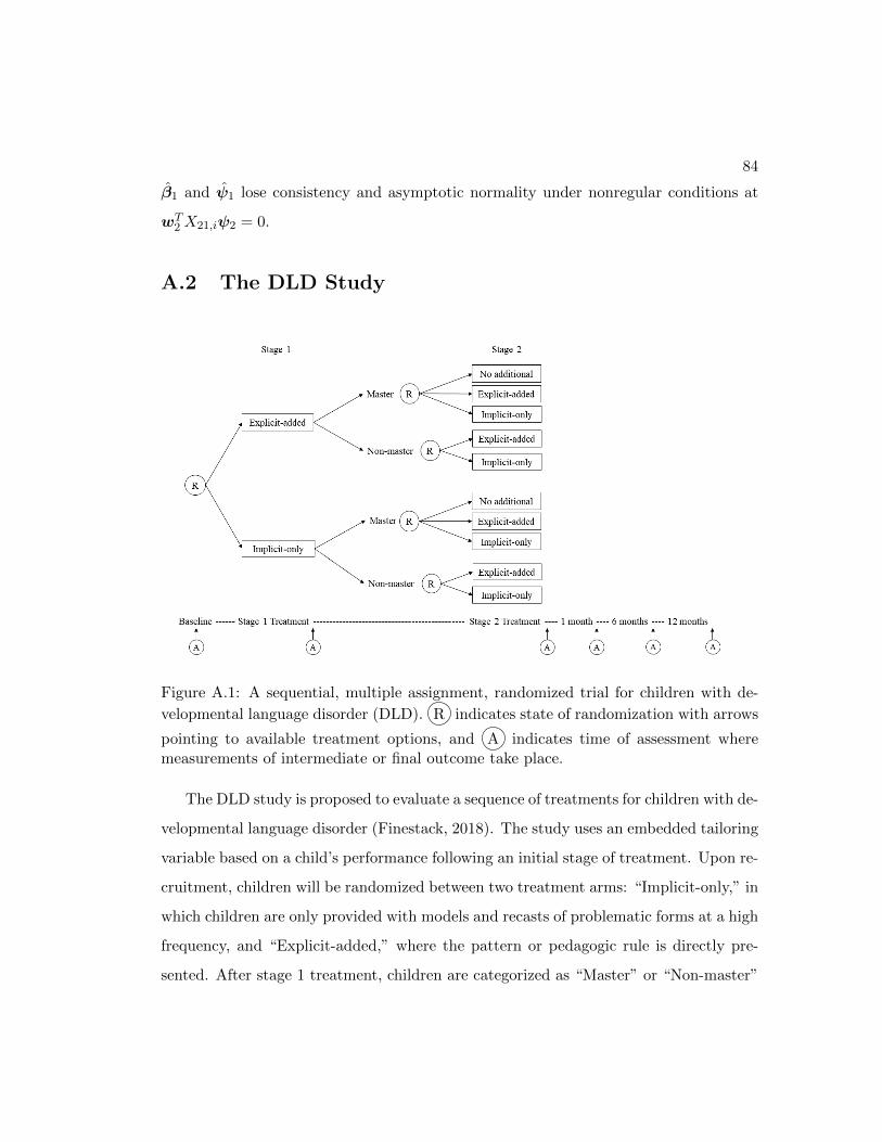
84

β1 and ψ1 lose consistency and asymptotic normality under nonregular conditions at

wT2 X21,iψ2 = 0.

A.2 The DLD Study

Figure A.1: A sequential, multiple assignment, randomized trial for children with de-

velopmental language disorder (DLD). R indicates state of randomization with arrows

pointing to available treatment options, and A indicates time of assessment wheremeasurements of intermediate or final outcome take place.

The DLD study is proposed to evaluate a sequence of treatments for children with de-

velopmental language disorder (Finestack, 2018). The study uses an embedded tailoring

variable based on a child’s performance following an initial stage of treatment. Upon re-

cruitment, children will be randomized between two treatment arms: “Implicit-only,” in

which children are only provided with models and recasts of problematic forms at a high

frequency, and “Explicit-added,” where the pattern or pedagogic rule is directly pre-

sented. After stage 1 treatment, children are categorized as “Master” or “Non-master”

85

based on their performance in target forms designed by the investigator. Masters will

be re-randomized to stop (“No additional”), boost (i.e., continue stage 1 treatment), or

switch to the alternative treatment, whereas non-masters will be randomized to boost or

switch. Similar to the M-bridge study, sustained performance after stage 2 is clinically

important; hence, the investigators also assess children’s performance at 1, 6, and 12

months after the treatment period.

A.3 Marginalization over an Unmeasured Covariate

Proposition 1. Suppose each element in a sequence of repeated-measures outcomes

(Y1, Y2, Y3) follows an independent normal distribution, Yij ∼ N(µj , σ2e) for subjects

i = 1, . . . , n and j = 1, 2, 3. Suppose the true mean µj is associated with a measurable

µj and an additional unmeasured covariate Vi ∼ N(0, σ2v) and µj = µj + λjVi. Then

the joint distribution of Y1, Y2, Y3 conditional on measurable µ1, µ2, µ3 is a multivariate

normal distribution with µ =(µ1 µ2 µ3

)Tand

Σ =

λ2

1σ2v + σ2

e λ1λ2σ2v λ1λ3σ

2v

λ1λ2σ2v λ2

2σ2v + σ2

e λ2λ3σ2v

λ1λ3σ2v λ2λ3σ

2v λ2

3σ2v + σ2

e

.

Proof. Since Y =(Y1 Y2 Y3

)T∼ MVN

(µ, σ2

eI3

), where µ =

(µ1 µ2 µ3

)Tand

I3 is a 3× 3 identity matrix, the joint distribution of (Y1, Y2, Y3) conditional on µ is

f(Y1, Y2, Y3|µ) =

∫ ∞−∞

f(Y1, Y2, Y3|µ, V )f(V |µ)dV

=

∫ ∞−∞

(2πσ2e)−3/2 exp

{− 1

2σ2e

(Y − µ)T (Y − µ)

}(2πσ2

v)−1/2 exp

{− 1

2σ2v

V 2

}dV

=

∫ ∞−∞

(2π)−2σ−3e σ−1

v exp

{− 1

2σ2e

(Y − µ)T (Y − µ)− 1

2σ2v

V 2

}dV,

86

where

(Y − µ)T (Y − µ) = (λ21 + λ2

2 + λ23)V 2 − 2V {λ1(Y1 − µ1) + λ2(Y2 − µ2) + λ3(Y3 − µ3)}

+ (Y1 − µ1)2 + (Y2 − µ2)2 + (Y3 − µ3)2.

Thus,

f(Y1, Y2, Y3|µ) =

∫ ∞−∞

(2π)−2σ−3e σ−1

v exp

{−1

2(aV 2 − 2bV + c)

}dV

= (2π)−3/2σ−3e σ−1

v a−1/2 exp

{−1

2(c− a−1b2)︸︷︷︸

ζ

}, (A.1)

where

a = σ−2e (λ2

1 + λ22 + λ2

3) + σ−2v

b = σ−2e {λ1(Y1 − µ1) + λ2(Y2 − µ2) + λ3(Y3 − µ3)}

c = σ−2e

{(Y1 − µ1)2 + (Y2 − µ2)2 + (Y3 − µ3)2

}.

The function indicated by ζ in Equation (A.1) can be expanded and simplified as

ζ = σ−2e

{Y 21 + Y 2

2 + Y 23 − 2µ1Y1 − 2µ2Y2 − 2µ3Y3 −

(λ1Y1 + λ2Y2 + λ3Y3 − λ1µ1 − λ2µ2 − λ3µ3)2

λ21 + λ22 + λ23 + σ2eσ−2v

}+ C

= σ−2e

3∑i=1

{1−

(λ21 + λ22 + λ23 + σ2

eσ−2v

)−1λ2i

}Y 2i − 2

3∑i=1

µi −(λ21 + λ22 + λ23 + σ2

eσ−2v

)−1λi

3∑j=1

λj µj

Yi

−(λ21 + λ22 + λ23 + σ2

eσ−2v

)−1 3∑i=1,i6=j

3∑j=1

λiλjYiYj

+ C.

Let ω =(λ2

1 + λ22 + λ2

3 + σ2eσ−2v

)−1. Therefore, by the definition of multivariate

normal distribution, the distribution of Y conditional on measurable covariates has

87

mean µ and precision matrix

Σ−1 = σ−2e

1− ωλ2

1 −ωλ1λ2 −ωλ1λ3

−ωλ1λ2 1− ωλ22 −ωλ2λ3

−ωλ1λ3 −ωλ2λ3 1− ωλ23

.

Finally, we obtain the desired covariance matrix by inverting the precision matrix.

A.4 Model Misspecifications in the Simulation Study

To apply Q-learning algorithms with GEE, we specify the Q-functions as

for t1 ∈ {1, 2, 3} and t2 ∈ {2, 3},

Qmis2 (H2, A2, t2;β2,ψ2) = β20,t2 + β21,t2Z1 + β22,t2A1 + β23,t2Y1

+A2 (ψ20,t2 + ψ21,t2Z1 + ψ22,t2A1 + ψ23,t2Y1) ,

Q2(H2, A2, t2;β2,ψ2) = β20,t2 + β21,t2Z1 + β22,t2A1 + β23,t2Z1A1 + β24,t2Y1

+A2 (ψ20,t2 + ψ21,t2Z1 + ψ22,t2A1 + ψ23,t2Y1) ,

Q1(H1, A1, t1;β1,ψ1) = β10,t1 + β11,t1Z1 +A1 (ψ10,t1 + ψ11,t1Z1) ;

whereas on the other hand, composite Q-learning fits

Qmis2 (H2, A2, t2;β2,ψ2) = β20 + β21Z1 + β22A1 + β23Y1

+A2 (ψ20 + ψ21Z1 + ψ22A1 + ψ23Y1) ,

Q2(H2, A2, t2;β2,ψ2) = β20 + β21Z1 + β22A1 + β23Z1A1 + β24Y1

+A2 (ψ20 + ψ21Z1 + ψ22A1 + ψ23Y1) ,

Q1(H1, A1, t1;β1,ψ1) = β10 + β11Z1 +A1 (ψ10 + ψ11Z1) .

88

A.5 Relative Efficiency Using Different Working Correla-

tions

Misspecification of working correlation structures in GEE can cause loss in efficiency.

In this section, we assess the relative efficiency of using “unstructured”, “exchangeable”

and “independent” working correlations in stage 1 estimation. Estimates are the same

under different correlation structures due to the inclusion of time-varying coefficients,

but standard errors are different. So we use variance instead of MSE to quantify ef-

ficiency. Table A.1 summarizes the ratio of variances of τj1(0) at time j, j = 1, 2, 3,

under different partial correlations. We assume there is not model misspecification in

this simulation. The λ’s specified in each scenario is summarized below:

1. Low positive partial correlation: λ1 = 1, λ2 = 0.2, λ3 = 0.2

2. Medium positive partial correlation: λ1 = 1, λ2 = 1, λ3 = 1

3. High positive partial correlation: λ1 = 1, λ2 = 3, λ3 = 1

4. Low negative partial correlation: λ1 = 1, λ2 = −0.2, λ3 = −0.2

5. Medium negative partial correlation: λ1 = 1, λ2 = −1, λ3 = −1

6. High negative partial correlation: λ1 = 1, λ2 = −3, λ3 = −1

7. Zero partial correlation: λ1 = 0, λ2 = 0, λ3 = 0

Note that “exchangeable” working correlation is the best choice for positive corre-

lations; “unstructured” working correlation is the best choice for negative correlations;

“independence” working correlation is the best choice for independent correlations.

Table A.1 shows that the relative efficiency does not change much across different

working correlations. For high positive partial correlations, “exchangeable” working

correlation seems to work slightly better than the other two options. For high negative

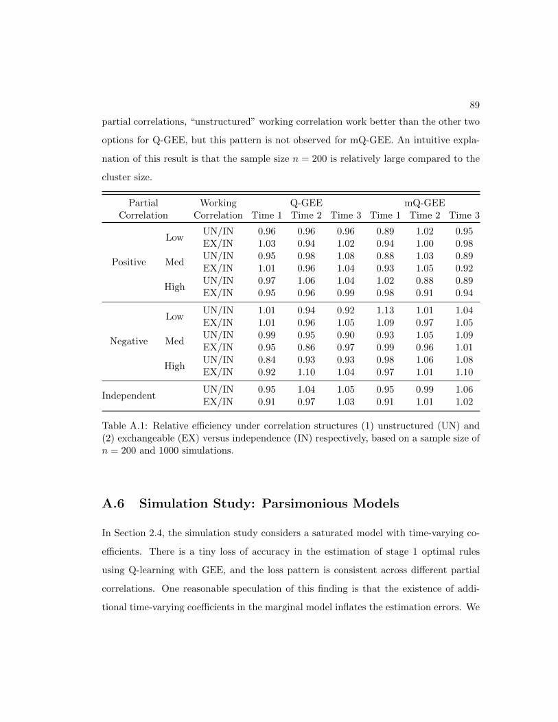
89

partial correlations, “unstructured” working correlation work better than the other two

options for Q-GEE, but this pattern is not observed for mQ-GEE. An intuitive expla-

nation of this result is that the sample size n = 200 is relatively large compared to the

cluster size.

Partial Working Q-GEE mQ-GEECorrelation Correlation Time 1 Time 2 Time 3 Time 1 Time 2 Time 3

Positive

LowUN/IN 0.96 0.96 0.96 0.89 1.02 0.95EX/IN 1.03 0.94 1.02 0.94 1.00 0.98

MedUN/IN 0.95 0.98 1.08 0.88 1.03 0.89EX/IN 1.01 0.96 1.04 0.93 1.05 0.92

HighUN/IN 0.97 1.06 1.04 1.02 0.88 0.89EX/IN 0.95 0.96 0.99 0.98 0.91 0.94

Negative

LowUN/IN 1.01 0.94 0.92 1.13 1.01 1.04EX/IN 1.01 0.96 1.05 1.09 0.97 1.05

MedUN/IN 0.99 0.95 0.90 0.93 1.05 1.09EX/IN 0.95 0.86 0.97 0.99 0.96 1.01

HighUN/IN 0.84 0.93 0.93 0.98 1.06 1.08EX/IN 0.92 1.10 1.04 0.97 1.01 1.10

IndependentUN/IN 0.95 1.04 1.05 0.95 0.99 1.06EX/IN 0.91 0.97 1.03 0.91 1.01 1.02

Table A.1: Relative efficiency under correlation structures (1) unstructured (UN) and(2) exchangeable (EX) versus independence (IN) respectively, based on a sample size ofn = 200 and 1000 simulations.

A.6 Simulation Study: Parsimonious Models

In Section 2.4, the simulation study considers a saturated model with time-varying co-

efficients. There is a tiny loss of accuracy in the estimation of stage 1 optimal rules

using Q-learning with GEE, and the loss pattern is consistent across different partial

correlations. One reasonable speculation of this finding is that the existence of addi-

tional time-varying coefficients in the marginal model inflates the estimation errors. We

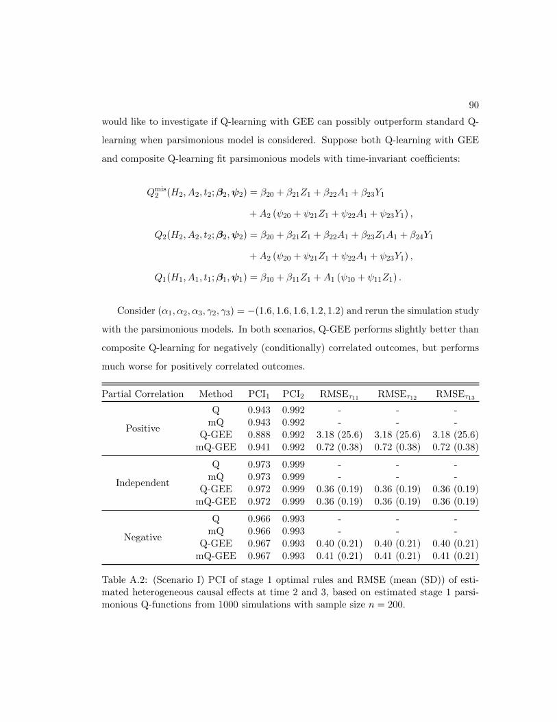
90

would like to investigate if Q-learning with GEE can possibly outperform standard Q-

learning when parsimonious model is considered. Suppose both Q-learning with GEE

and composite Q-learning fit parsimonious models with time-invariant coefficients:

Qmis2 (H2, A2, t2;β2,ψ2) = β20 + β21Z1 + β22A1 + β23Y1

+A2 (ψ20 + ψ21Z1 + ψ22A1 + ψ23Y1) ,

Q2(H2, A2, t2;β2,ψ2) = β20 + β21Z1 + β22A1 + β23Z1A1 + β24Y1

+A2 (ψ20 + ψ21Z1 + ψ22A1 + ψ23Y1) ,

Q1(H1, A1, t1;β1,ψ1) = β10 + β11Z1 +A1 (ψ10 + ψ11Z1) .

Consider (α1, α2, α3, γ2, γ3) = −(1.6, 1.6, 1.6, 1.2, 1.2) and rerun the simulation study

with the parsimonious models. In both scenarios, Q-GEE performs slightly better than

composite Q-learning for negatively (conditionally) correlated outcomes, but performs

much worse for positively correlated outcomes.


Positive

Q 0.943 0.992 - - -mQ 0.943 0.992 - - -

Q-GEE 0.888 0.992 3.18 (25.6) 3.18 (25.6) 3.18 (25.6)mQ-GEE 0.941 0.992 0.72 (0.38) 0.72 (0.38) 0.72 (0.38)

Independent

Q 0.973 0.999 - - -mQ 0.973 0.999 - - -

Q-GEE 0.972 0.999 0.36 (0.19) 0.36 (0.19) 0.36 (0.19)mQ-GEE 0.972 0.999 0.36 (0.19) 0.36 (0.19) 0.36 (0.19)

Negative

Q 0.966 0.993 - - -mQ 0.966 0.993 - - -

Q-GEE 0.967 0.993 0.40 (0.21) 0.40 (0.21) 0.40 (0.21)mQ-GEE 0.967 0.993 0.41 (0.21) 0.41 (0.21) 0.41 (0.21)

Table A.2: (Scenario I) PCI of stage 1 optimal rules and RMSE (mean (SD)) of esti-mated heterogeneous causal effects at time 2 and 3, based on estimated stage 1 parsi-monious Q-functions from 1000 simulations with sample size n = 200.

91


Positive

Q 0.930 0.996 - - -mQ 0.945 0.996 - - -

Q-GEE 0.871 0.996 3.47 (26.8) 3.47 (26.8) 3.47 (26.8)mQ-GEE 0.943 0.996 0.71 (0.37) 0.71 (0.37) 0.71 (0.37)

Independent

Q 0.943 0.998 - - -mQ 0.969 0.998 - - -

Q-GEE 0.911 0.998 1.93 (3.33) 1.93 (3.33) 1.93 (3.33)mQ-GEE 0.968 0.998 0.42 (0.22) 0.42 (0.22) 0.42 (0.22)

Negative

Q 0.782 0.977 - - -mQ 0.960 0.977 - - -

Q-GEE 0.824 0.977 2.39 (0.40) 2.39 (0.40) 2.39 (0.40)mQ-GEE 0.962 0.977 0.49 (0.25) 0.49 (0.25) 0.49 (0.25)

Table A.3: (Scenario II) PCI of stage 1 optimal rules and RMSE of estimated het-erogeneous causal effects at time 2 and 3, based on estimated stage 1 parsimoniousQ-functions from 1000 simulations.

A.7 Application: Model Fit and Variable Selection

We performed constrained variable selection based on QIC for both stage 1 and stage 2

saturated models (with time-varying coefficients), where the time-dependent effects of

A1 are forced in the stage 1 model and the time-dependent effects of A2 and A1 ∗A2 are

forced in the stage 2 model. Table A.4 shows a summary of the estimated parameters

using mQ-GEE, assuming equal weights for all three outcome measurements.

Table A.4: Summary of stage 1 model and stage 2 model with variable selection.

Estimate SE p-value1

Stage 1 Model

Main Effects

Continued on next page1* p < 0.05, ** p < 0.01, *** p < 0.001

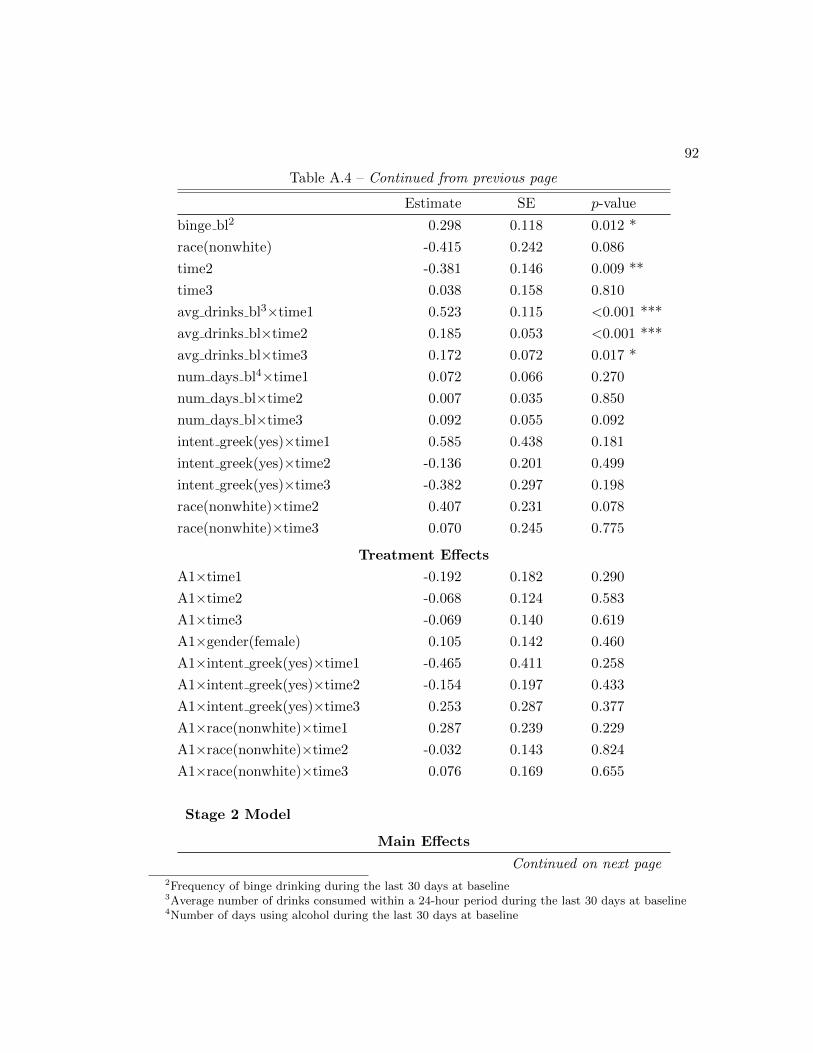
92

Table A.4 – Continued from previous page

Estimate SE p-value

binge bl2 0.298 0.118 0.012 *

race(nonwhite) -0.415 0.242 0.086

time2 -0.381 0.146 0.009 **

time3 0.038 0.158 0.810

avg drinks bl3×time1 0.523 0.115 <0.001 ***

avg drinks bl×time2 0.185 0.053 <0.001 ***

avg drinks bl×time3 0.172 0.072 0.017 *

num days bl4×time1 0.072 0.066 0.270

num days bl×time2 0.007 0.035 0.850

num days bl×time3 0.092 0.055 0.092

intent greek(yes)×time1 0.585 0.438 0.181

intent greek(yes)×time2 -0.136 0.201 0.499

intent greek(yes)×time3 -0.382 0.297 0.198

race(nonwhite)×time2 0.407 0.231 0.078

race(nonwhite)×time3 0.070 0.245 0.775

Treatment Effects

A1×time1 -0.192 0.182 0.290

A1×time2 -0.068 0.124 0.583

A1×time3 -0.069 0.140 0.619

A1×gender(female) 0.105 0.142 0.460

A1×intent greek(yes)×time1 -0.465 0.411 0.258

A1×intent greek(yes)×time2 -0.154 0.197 0.433

A1×intent greek(yes)×time3 0.253 0.287 0.377

A1×race(nonwhite)×time1 0.287 0.239 0.229

A1×race(nonwhite)×time2 -0.032 0.143 0.824


Stage 2 Model

Main Effects

Continued on next page2Frequency of binge drinking during the last 30 days at baseline3Average number of drinks consumed within a 24-hour period during the last 30 days at baseline4Number of days using alcohol during the last 30 days at baseline

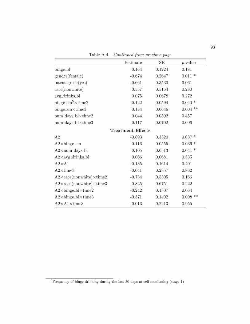
93

Table A.4 – Continued from previous page

Estimate SE p-value

binge bl 0.164 0.1224 0.181

gender(female) -0.674 0.2647 0.011 *

intent greek(yes) -0.661 0.3530 0.061

race(nonwhite) 0.557 0.5154 0.280

avg drinks bl 0.075 0.0678 0.272

binge sm5×time2 0.122 0.0594 0.040 *

binge sm×time3 0.184 0.0646 0.004 **

num days bl×time2 0.044 0.0592 0.457

num days bl×time3 0.117 0.0702 0.096

Treatment Effects

A2 -0.693 0.3320 0.037 *

A2×binge sm 0.116 0.0555 0.036 *

A2×num days bl 0.105 0.0513 0.041 *

A2×avg drinks bl 0.066 0.0681 0.335

A2×A1 -0.135 0.1614 0.401

A2×time3 -0.041 0.2357 0.862

A2×race(nonwhite)×time2 -0.734 0.5305 0.166


A2×binge bl×time2 -0.242 0.1307 0.064

A2×binge bl×time3 -0.371 0.1402 0.008 **

A2×A1×time3 -0.013 0.2213 0.955

5Frequency of binge drinking during the last 30 days at self-monitoring (stage 1)

Appendix B

Supplementary Materials for mIQ

B.1 Proof

Theorem 3.3.1 (Matrix Version of the Omitted Variable Bias Theorem). Suppose

that the true regression model for Y is Y = ψ0 + XTψ1 + V Tγ + ε, where X is a

random vector formed by measured covariates, V is formed by unmeasured covariates,

and ε ∼ N(0, σ2). The parameters associated with measured covariates, ψ ≡

ψ0

ψ1

,

are thus estimated via the misspecified model y = β0 + xTβ1 + ε∗, where y and x are

realizations of Y and X respectively. Then

E(β) ≡ E

β0

β1

= ψ +


Cov(X)−1Cov(X,V )

γ.Theorem 3.3.1 is developed based on the omitted variable formula and example in

Econometric Analysis by Greene (2002).

Proof. Let X denote a design matrix with xTi as the ith row, i = 1, . . . , n and y denote

a vector with yi as the ith element. Suppose that V is observable and let V denote

94

95

a matrix with vi, a realization of V , as the ith row. Define X =(1 X

). The least

squares estimator of β is β = (XT X)−1XTy.

E(β) = ψ + E[(XT X)−1XTV

]γ.

Consider the multivariate regression V = λ0 +Λ1x+ε∗∗, where ε∗∗ ∼MVN(0,Σ).

The least squares estimator of Λ =

λT0ΛT

1

is Λ = (XT X)−1XTV. Hence, E[(XT X)−1XTV

]=

E(Λ) = Λ and E(β) = ψ + Λγ. Now, it remains to prove that

Λ =


Cov(X)−1Cov(X,V )

.

The true values of Λ satisfy the equation

(λ0,Λ1) = arg minΛ

E(V − λ0 −Λ1X)T (V − λ0 −Λ1X) = arg minΛ

L.

The first derivative of L with respect to (λ0,Λ1) is

∂L

∂λ0= −2E(V T ) + 2λT0 + 2E(XT )ΛT

1 ,

∂L

∂Λ1= −2E(XV T ) + 2E(X)λT0 + 2E(XXT )ΛT

1 .

Hence, the score equations of (λ0,Λ1) are

S(λ0) = λ0 − E(V T ) + E(XT )ΛT1 = 0,

S(Λ1) =[E(XXT )− E(X)E(XT )

]ΛT

1 −[E(XV T )− E(X)E(V T )

]= Cov(X)ΛT

1 − Cov(X,V ) = 0

Therefore, ΛT1 = Cov(X)−1Cov(X,V ) and λT0 = E(V T )−E(XT )Cov(X)−1Cov(X,V ).

96

Theorem 3.3.2 (Bias of Stage 2 Treatment Effect Estimators). Assume that V20 is a

vector of unmeasured covariates that are independent of A2 and Cov(X2) is invertible.

The estimators of stage 2 heterogeneous treatment effects are unbiased if and only if at

least one of the following conditions is satisfied:

• E(A2) = 0;

• V20 is correlated with neither X20 nor X21.

Proof. By Theorem 3.3.1, we know that the bias of β2 =(βT201 β210 βT211

)Tis

Bias(β2) = Cov(X2)−1Cov(X2,V20)γ20 = Cov(X2)−1

Cov(X20,V20)

0T

E(A2)Cov(X21,V20)

γ20.

Suppose E(A2) 6= 0. Since Cov(X2) is invertible, we have

Bias(β2) = 0⇐⇒

Cov(X20,V20)

0T

E(A2)Cov(X21,V20)

= 0⇐⇒ Cov(X20,V20) = 0 and Cov(X21,V20) = 0.

Suppose E(A2) = 0. Note that Cov(X20, A2X21) = E(A2)Cov(X20,X21) = 0.

Rewrite Cov(X2) as a partitioned matrix:

Cov(X2) = Cov

X20

A2

A2X21

=

Cov(X20) Cov(X20, A2) Cov(X20, A2X21)

Cov(A2,X20) Var(A2) Cov(A2, A2X21)

Cov(A2X21,X20) Cov(A2X21, A2) Cov(A2X21)

97

=

Cov(X20) 0 0

0T Var(A2) Var(A2)E(XT21)

0T Var(A2)E(X21) Cov(A2X21)

.

Let P =

Var(A2) Var(A2)E(XT21)

Var(A2)E(X21) Cov(A2X21)

.

Then Cov(X2)−1 =

Cov(X20)−1 0T

0 P−1

. It follows that

E(A2) = 0⇐⇒ Bias

β210

β211

= P−1

0

E(A2)Cov(X21,V20)

= 0.

Therefore, the estimators of stage 2 treatment effects, β210 and β211, are unbiased if

and only if E(A2) = 0 or Cov(X20,V20) = Cov(X21,V20) = 0.

Theorem 3.3.3 (Bias of Stage 2 Main Effect Estimators). Assume that V20 is a vector

of unmeasured covariates that are independent of A2 and E(A2) = 0. Suppose that V20

is correlated with X20 and Cov(X2) is invertible. Then the estimators of stage 2 main

effects are biased and the bias is B′γ20, where

B′ =

E(V T20)− E(XT

2 )Cov(X2)−1Cov(X2,V20)


. (3.7)

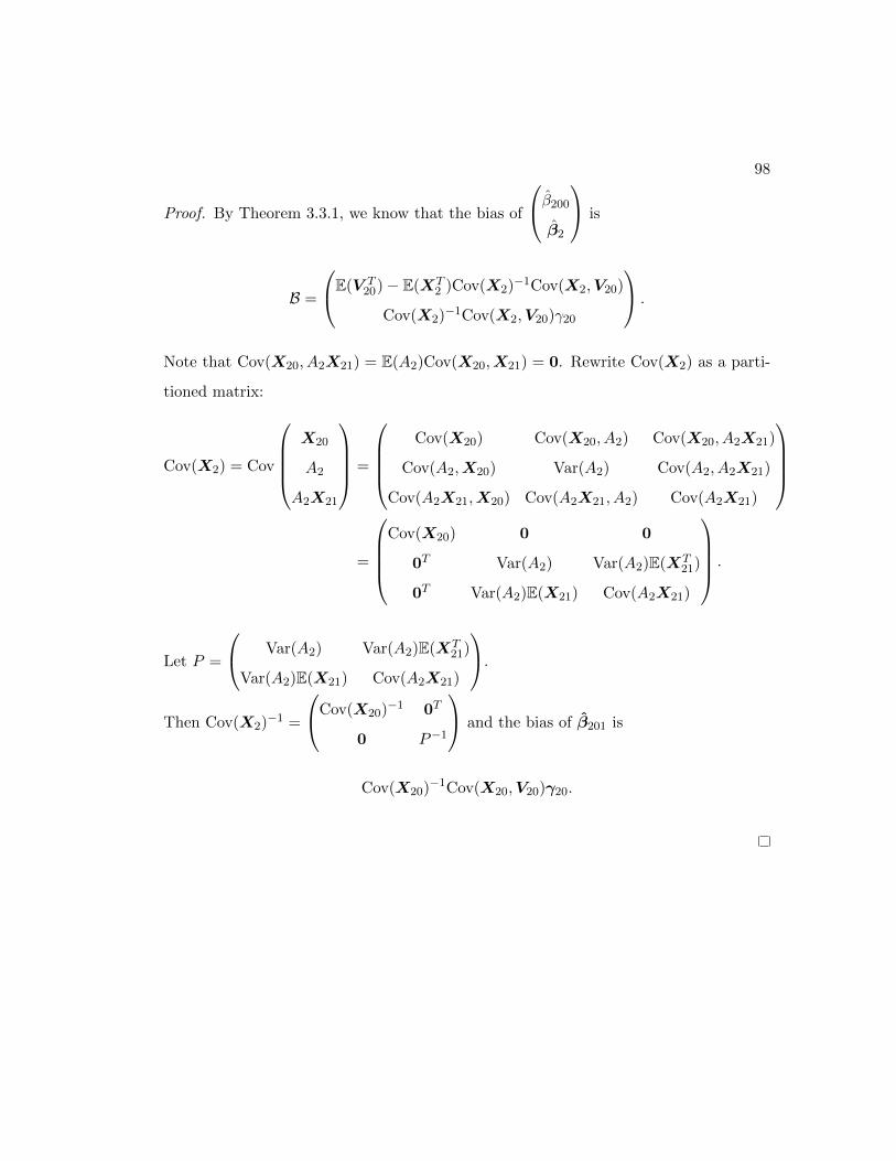
98

Proof. By Theorem 3.3.1, we know that the bias of

β200

β2

is

B =

E(V T20)− E(XT

2 )Cov(X2)−1Cov(X2,V20)

Cov(X2)−1Cov(X2,V20)γ20

.

Note that Cov(X20, A2X21) = E(A2)Cov(X20,X21) = 0. Rewrite Cov(X2) as a parti-

tioned matrix:

Cov(X2) = Cov

X20

A2

A2X21

=

Cov(X20) Cov(X20, A2) Cov(X20, A2X21)

Cov(A2,X20) Var(A2) Cov(A2, A2X21)

Cov(A2X21,X20) Cov(A2X21, A2) Cov(A2X21)

=

Cov(X20) 0 0

0T Var(A2) Var(A2)E(XT21)

0T Var(A2)E(X21) Cov(A2X21)

.

Let P =

Var(A2) Var(A2)E(XT21)

Var(A2)E(X21) Cov(A2X21)

.

Then Cov(X2)−1 =

Cov(X20)−1 0T

0 P−1

and the bias of β201 is

Cov(X20)−1Cov(X20,V20)γ20.

99

Theorem 3.4.1. Suppose X ∼ N(µ, σ2). Then

E(|X|) =

(2σ2

π

) 12

exp

(− µ2

2σ2

)+ µ

{1− 2Φ

(−µσ

)}.

Proof. Let f(x) and F (x) be the probability density function and the cumulative dis-

tribution function of X respectively. Then

E(|X|) =

∫ 0

−∞−xf(x)dx+

∫ ∞0

xf(x)dx

= 2

∫ ∞0

xf(x)dx− µ

= 2

∫ ∞0

(x− µ)f(x)dx+ 2µ

∫ ∞0

f(x)dx− µ

= 2

∫ ∞0

(x− µ)(2πσ2

)− 12 exp

{− 1

2σ2(x− µ)2

}dx+ 2µ

{1− F (0)

}− µ

= 2

[−σ2

(2πσ2

)− 12 exp

{− 1

2σ2(x− µ)2

}]∞0

+ 2µ{

1− Φ(−µσ

)}− µ

=

(2σ2

π

) 12

exp

(− µ2

2σ2

)+ µ

{1− 2Φ

(−µσ

)}.

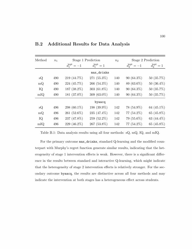
100

B.2 Additional Results for Data Analysis

Method n1 Stage 1 Prediction n2 Stage 2 Prediction

dopt1 = −1 dopt

1 = 1 dopt2 = −1 dopt

2 = 1

max_drinks

sQ 490 219 (44.7%) 271 (55.3%) 140 90 (64.3%) 50 (35.7%)

mQ 490 224 (45.7%) 266 (54.3%) 140 89 (63.6%) 50 (36.4%)

IQ 490 187 (38.2%) 303 (61.8%) 140 90 (64.3%) 50 (35.7%)

mIQ 490 181 (37.0%) 309 (63.0%) 140 90 (64.3%) 50 (35.7%)

byaacq

sQ 496 298 (60.1%) 198 (39.9%) 142 78 (54.9%) 64 (45.1%)

mQ 496 261 (52.6%) 235 (47.4%) 142 77 (54.2%) 65 (45.8%)

IQ 496 237 (47.8%) 259 (52.2%) 142 79 (55.6%) 63 (44.4%)

mIQ 496 229 (46.2%) 267 (53.8%) 142 77 (54.2%) 65 (45.8%)

Table B.1: Data analysis results using all four methods: sQ, mQ, IQ, and mIQ.

For the primary outcome max_drinks, standard Q-learning and the modified coun-

terpart with Murphy’s regret function generate similar results, indicating that the het-

erogeneity of stage 1 intervention effects is weak. However, there is a significant differ-

ence in the results between standard and interactive Q-learning, which might indicate

that the heterogeneity of stage 2 intervention effects is relatively stronger. For the sec-

ondary outcome byaacq, the results are distinctive across all four methods and may

indicate the intervention at both stages has a heterogeneous effect across students.

Appendix C

Supplementary Materials for

mLQ

C.1 The Manifest Distribution

In the latent variable formulation of probit regression, the joint distribution of Y and

Y ∗ is:

f(yi, y∗i |µ, σ) = f(y∗i |µi, σ)p(yi|y∗i )

= (2πσ2)−1/2 exp

{− 1

2σ2(y∗i − µi)2

}[1{yi = 1}1{y∗i > ξ}

+ 1{yi = 0}1{y∗i ≤ ξ}]

= (2πσ2)−1/2 exp

{− 1

2σ2(y∗i − µ)2

}[yi1{y∗i > ξ}+ (1− yi)1{y∗i ≤ ξ}

]where f denotes the probability density function and p denotes the probability mass

function.

The manifest distribution, or the marginal distribution of the response variable Y ,

101

102

conditional on model covariates H2 and A2, is

p(yi|H2i, A2i) =

∫ ∞−∞

p(yi|y∗i , H2i, A2i)f(y∗i |H2i, A2i)dy∗i

= yi

∫ ∞ξ

f(y∗i |H2i, A2i)dy∗i + (1− yi)

∫ ξ

−∞f(y∗i |H2i, A2i)dy

∗i

= yi

{1− Φ

(ξ − xT20,iβ20 − a2ix

T21,iβ21

σ

)}

+ (1− yi)Φ

(ξ − xT20,iβ20 − a2ix

T21,iβ21

σ

),

where Φ is the cumulative distribution function of a standard normal random variable.

C.2 Conditional Moments of the Latent Variable

In order to construct the EM algorithm, we need to derive the first and second moments

of the latent variable Y ∗ conditional on the manifest variable Y . As the value of Y

implies the truncation range of Y ∗, the distribution of Y ∗ conditional on Y is a truncated

normal distribution. The first moment, i.e. the expectation, of Y ∗ conditional on Y is

E (Y ∗|Y ) = µ+(2Y − 1)σ2φ(µ, σ2; ξ)

Y {1− Φ(µ, σ2; ξ)}+ (1− Y )Φ(µ, σ2; ξ), (C.1)

and the second moment of Y ∗ conditional on Y is

E(Y ∗2

∣∣Y ) = µ2 + σ2 +(2Y − 1)(µ+ ξ)σ2φ(µ, σ2; ξ)

Y {1− Φ(µ, σ2; ξ)}+ (1− Y )Φ(µ, σ2; ξ), (C.2)

where φ(µ, σ2) and Φ(µ, σ2) denote the probability density function and cumulative

distribution function of N(µ, σ2) respectively.

We show the derivation of Equations (C.1) and (C.2) for the case of Y = 1 only,

and the derivation for the case of Y = 0 can be done similarly.

103

E (Y ∗|Y = 1) =1

1− Φ(µ, σ2; ξ)

∫ ∞ξ

y∗(2πσ2)−1/2 exp

{− 1

2σ2(y∗ − µ)2

}dy∗

=1

1− Φ(µ, σ2; ξ)

{−σ2

[(2πσ2)−1/2 exp

{− 1

2σ2(y∗ − µ)2

}]∞ξ

+

∫ ∞ξ

µf(y∗)dy∗}

=σ2φ(µ, σ2; ξ) + µ

{1− Φ(µ, σ2; ξ)

}1− Φ(µ, σ2; ξ)

= µ+ σ2 φ(µ, σ2; ξ)

1− Φ(µ, σ2; ξ)

E(Y ∗2

∣∣Y = 1)

=1

1− Φ(µ, σ2; ξ)

∫ ∞ξ

y∗2(2πσ2)−1/2 exp

{− 1

2σ2(y∗ − µ)2

}dy∗

=1

1− Φ(µ, σ2; ξ)

{∫ ∞ξ

y∗(y∗ − µ)(2πσ2)−1/2 exp

{− 1

2σ2(y∗ − µ)2

}dy∗

+ µ[µ{

1− Φ(µ, σ2; ξ)}

+ σ2φ(µ, σ2; ξ)]}

=1

1− Φ(µ, σ2; ξ)

{[−σ2y∗(2πσ2)−1/2 exp

{− 1

2σ2(y∗ − µ)2

}]∞ξ

+

∫ ∞ξ

σ2(2πσ2)−1/2 exp

{− 1

2σ2(y∗ − µ)2

}dy∗

+ µ[µ{

1− Φ(µ, σ2; ξ)}

+ σ2φ(µ, σ2; ξ)]}

=1

1− Φ(µ, σ2; ξ)

[σ2ξφ(µ, σ2; ξ) + σ2

{1− Φ(µ, σ2; ξ)

}+ µ2

{1− Φ(µ, σ2; ξ)

}+ µσ2φ(µ, σ2; ξ)

]= µ2 + σ2 + (µ+ ξ)σ2 φ(µ, σ2; ξ)

1− Φ(µ, σ2; ξ)

Modi cations of Q-learning to Optimize Dynamic Treatment ...

Documents

Transcript of Modi cations of Q-learning to Optimize Dynamic Treatment ...