MODERN SAMPLED-DATA CONTROL THEORY: Design of the … · 2013-08-31 · NASA CONTRACTOR REPORT NASA...

N A S A C O N T R A C T O R

R E P O R T

N A S A C R - 2 4 5 7

wo

MODERN SAMPLED-DATA CONTROL THEORY:

Design of the Large Space Telescope

by B. C. Kuo and G. Singh

Prepared by

SYSTEMS RESEARCH LABORATORY

Champaign, 111. 61820

for George C, Marshall Space Flight Center

NATIONAL AERONAUTICS AND SPACE ADMINISTRATION • WASHINGTON, D. C. • SEPTEMBER 1974

https://ntrs.nasa.gov/search.jsp?R=19750002803 2020-03-11T07:52:59+00:00Z

TECHNICAL REPORT STANDARD TITLE PAGE'1. REPORT NO.

NASA CR- 24572. GOVERNMENT ACCESSION NO. 3. RECIPIENT'S CATALOG NO.

4. TITLE AND SUBTITLE

MODERN SAMPLED-DATA CONTROL THEORY:Design of the Large Space Telescope

5. REPORT DATESeptember

6. PERFORMING ORGANIZATION CODE

M1327. AUTHOR(S)

B. C. Kuo and G. Singh8. PERFORMING ORGANIZATION REPORT #

9. PERFORMING ORGANIZATION NAME AND ADDRESS

Systems Research LaboratoryP. O. Box 2277, Station AChampaign, Illinois 61820

10. WORK UNIT NO.

1 1. CONTRACT OR GRANT NO.

NAS 8-29853

12. SPONSORING AGENCY NAME AND ADDRESS

National Aeronautics and Space AdministrationWashington, D. C. 20546

13; TYPE OF REPORT ft PERIOD COVERED

CONTRACTORFinal

. SPONSORING AGENCY CODE

15. SUPPLEMENTARY NOTES

16. ABSTRACT

This investigation was undertaken to determine the effect of varying the sampling periodon the dynamic response of the sampled-data LST system.

A range of sampling periods is recommended based on the criterion that self-sustainedoscillations are to be avoided in the LST system. The step responses of the LST systemare then investigated when various sampling periods are used.

For small sampling periods, the dynamic behavior of the sampled-data system is verysimilar to that of the continuous-data system. When T is large (but less than 0.25 sec) theovershoot of the step response of the sampled-data system becomes greater. However,the dynamic behavior of the sampled-data system may be improved by redesigningthe controller.

From this study it appears that a sampling period as high as 0.1 second is feasible forthe LST system. However, it should be noted that the conclusions are obtained with theexisting system model. Other practical considerations such as noise, coupling effects andquantization errors, may restrict the sampling period to a lower value.

17. KEY WORDS 18. DISTRIBUTION STATEMENT

CAT. 109. SECURITY CLASSIF. (of thU report)

Unclassified20. SECURITY CLASSIF. (of thia page)

Unclassified21. NO. OF PAGES

13122. PRICE

MsFC- Form 3 293 (Rev December 1971) For sale by National Technical Information Service, Springfield, Virginia 12151

TABLE OF CONTENTS

1. Selecting the Sampling Period of the 1ST System . 1

2. Design of the Continuous-Data LST System 18

3. Computer Simulation of the Simplified LST SystemWith the Linear State Regulator and EigenvalueAssignment Designs 32

4. Digital Redesign of the Large Space Telescope (LST)System 40

5. Stability Considerations and Constraints on the Selectionof the Weighting Matrix of the Digital Redesign Technique 76

6. Realization of State Feedback by Dynamic Controllers 84

7. A Numerical Technique for Predicting Self-SustainedOscillations in the-Nonlinear 1ST System With theContinuous and Discrete Describing Function Methods 106

References 128

iii

1. Selecting the Sampling Period of the LSI System

The objective of this investigation is to determine the effect of

varying the sampling period on the dynamic response of the sampled-

data LSI system.

A range of sampling periods is recommended based on the criterion

that self-sustained oscillations are to be avoided in the LSI system.

The step responses of the LST system are then investigated when various

sampling periods are used.

Detailed description of the LST system with the CMG nonlinearity

is available in the Final Report, CONTINUOUS AND DISCRETE DESCRIBING

FUNCTION ANALYSIS OF THE LST SYSTEM, January 1, 1974, prepared by the

authors for NASA, Huntsville, under contract NAS8-29853. In that report

describing function analyses are applied to the continuous-data and the

sampled-data models of the LST system with the CMG nonlinearity. It is

shown that the 9th-order LST system can be closely approximated by a

4th-order system.

Two sets of system parameters (System 1 and System 2) were considered

in the Final Report. The study included in this report is concerned only

with System 1.

It has been established that for System 1, and with y = 1-38 x 10

for the CMG nonlinearity, self-sustained oscillations will occur if the

sampling period T exceeds 0.25 sec approximately.

In order to carry out the discrete describing function analysis for

the sampled-data system, a sampler is inserted in the nonlinear loop, and

thus a two-sampler system results. Computer simulation results show that

2

the two-sampler model gives very good predictions on the occurance of self-

sustained oscillations in the one-sampler system by the discrete describing

function analysis.

Figures 1-1 and 1-2 show the zero-input responses of the LSI system

with two samplers; Figures 1-3 and 1-4 show the responses when there is

only one sampler in the system. In both cases, the initial value of 6y8 *(vehicle position) is 5 * 10~ rad while all other initial conditions are

zero. The sampling period is 0.25 sec. With this large sampling period,

the system actually settles into a self-sustained oscillation with a

peak value of 0V approximately equal to 10" rad, although this amplitude

is not visible from the curves of Figures 1-1 through 1-4. As mentioned

earlier, the sampling period of T = 0.25 sec can be considered as a

boundary case between stability and instability.

It is of interest to investigate the step response of the LSI system-8with and without sampling. A step input of amplitude 5 x 10 K is applied

-8which yields a final value of 5 * 10 rad for 6... Figures 1-5 and 1-6

illustrate the step responses of the continuous-data LSI system. As

expected, the continuous-data LSI system with the designated controlle.-

parameter K and K, has a fairly good step response, since it was demonstrated

that the system has a relative damping ratio of 70% approximately.

Figures 1-7 through 1-12 show the step responses of the sampled-data

system with one sampler when T = 0.05, 0.1, and 0.25 sec, respectively.

Figures 1-13 and 1-14 show the step responses of the two-sampler system

with T = 0.25 sec:

When T = 0.25 sec, the step responses again have small oscillations in

the steady state.

The step responses in Figures 1-5 through 1-14 show that the LSI

system with a step input behaves very similar (except for a shift in

the reference of 9..) to the system with zero input and nonzero initial

value for 6,,.

The stability characteristics of the system with step input are

also very similar to those of the system with zero input.' ' . ' ' - . ' • • - • • ' • c . . ' • • •

The conclusion is that with y = 1.38 x 10 , the continuous-data

system is always stable while the sampled-data system is stable for T

less than 0.25 sec.

For small sampling periods, the dynamic behavior of the sampled-

data system is very similar to that of the continuous-data system. When

T is large (but less than 0.25 sec) the overshoot of the step response

of the sampled-data system becomes greater. However, the dynamic behavior

of the sampled-data system may be improved by redesigning the controller.

From this study it appears that a sampling period as high as 0.1

second is feasible for the LST system. However, it should be noted that

the conclusions are obtained with the existing system model. Other

practical considerations such as noise, coupling effects and quantization

errors, may restrict the sampling period to a lower value.

System 1, y = l-38xlOs T = 0.25 sec

Two Samplers

o

•CD-CD

O.l

0.00I ' I ' I T T

1.50 3.00 U.50 6.00TIME

7.50

fe I:X

>

o.I

0.00i • i • l ^ r • i

1.50 3.00 4.50 6.00 7.50

TIME

7.50

Figure 1-1

CD

f HCD3 fM

en

CD.I

System 1, Y = 1.38xlOs T = 0.25 sec

Two Samplers

0.00I ' I ' I ' I ' I

1.50 3;00 ii.50 6.00 7.50TIME

CO O

i \r>o •_•- rsix

oIf)c-=»•.

0.00r ' n ' i

1.50 3,00 4.50TIME

6.00 7.50

0.00

Figure 1-2

6

0.00

System 1, y = 1.38xl05 T = 0.25 secOne Sanpler

7.50

a-

o*-

O .T O '

o.I

0.00I ^ I • ' F I T

1.50 3.00 H.50 6.00 7.50TIME

0.00I ' r-- I

1.50 3.00 U.50T I M E

6.00 7.50

Figure 1-3

0.00

System 1, Y = 1.38><10S T * 0.25 sec

One Sampler

.00 1.50 3.001 •

4.50 6.00l

7.50TIME

a. oo 7.50

Figure 1-4

System 1, Y = 1.38xl05 No Sampler

o6'

--^ inf 8

X>

<D

O

o"0.00 1.50 3.00 4.50 6.00

TIME7.50

1 Ia.00 LSD

I r I ,3.00 U.50

TIME

. I I6.00 7.50

D.OO 1.50 3.00 U.50:

TIME

I rrT I6.00 . 7.50

Figure 1-5

System 1, Y= 1.38*105 No Sampler

1 i r r • i ^ i •> * i0.00 1.50 3.00 4.50 6.00 7.50

TIME . ...

0.00r • i • r^ ^^ i T . T

1.50 3.00 4.50 6.00 7.50TIME

D.OOI ' I ' \ ' t. ' i

1.50 3.00 4.50 6.00 7.50TIME

Figure 1-6

10

ino

o u»i— OJx o

oo

System 1, y = 1.38x10* T = 0.05 sec• : • • ' • - •

One Sampler

0.00i T i ' -i ' ^^ ^ I

1.50 3.00 4.50 6.00 7.50T I M E

0.00I ' I I ' I * I

1.50 3.00 11,50 6.00 7,50 5TIME

0.00 1.50 3^10 14.50 6.00 7.50TIME

Fiqure 1-7

0.00

System 1, Y = 1.38*105 T = 0.05 sec

One Sampler

11

T I r i T r T r1.50 3.00 4.50 6.00

TIME7.50

0.00^ n ' i • r T r1.50 3.00 4.50 6.00

TIME7.50

i.o

0.00 1.50 3.00 4.50 6.00T I M E

7.50

Finure 1-8

12

CDO

o rr

Oo

0.00

System 1, y = 1.38*105 T = 0.1 sec

One Sampler

i • i r r ' I1.50 3.00 4.50 6.00

TIME7.50

0.00I ^ I ' I ' I

1.50 3.00 4.50 6.00TIME

7.50

o.qo 1.50 3.00 U.50 6.00TIME

I7.50

Figure 1-9

System 1, y " 1.38x]05 T s 0.1 sec

One Sampler13

in

o.

0.00 1.50 3.00 U.50TIME

6.00 7.50

1oX

"u.ID

*-\

8."enCMl i • i ' • i ' r ' i

0.00 1.50 3.00 U.50 6.00 7.50TIME

0.00I ^ I ' I ' I ' I

1.50 3.00 U.SO 6.00 7.50TIME

Fiqure 1-10

14

COO

CD'

OO

0.00

System 1, y = 1.38xl05 T = 0.25 secOne Sampler

1.50 3.00 U.50 6.00TIME

7.50

tno

O.

0.00~n '— i • T • i1.50 3.00 4.50 6,00

TIME7.50

o.oa 1.50 3.00 U,50TIME

6.00 7.50

Fiqure 1-11

0.00

System 1, y = 1.38*105; T = 0.25 sec

One Sampler

15

1.50 3.00 4.50TIME

o10

•rso «J.'T I

orro- uo-

0.00 1.50 3.00 ii.50 6.00 7.50TIME

0.00

Figure 1-12

16

CDo

§• M

o0.00

System 1, y = 1.38*105 T - 0.25 secTwo Samplers

1.50 3.00 U.50 6.00 7.50TIME

« oo d:"x

3TS

0.00 1.50 3.00 4.50TIME

6.00 7.50

0.00

Figure 1-13

en<M

System 1, Y - 1.38*105 T = 0.25 sec

Two Samplers

o o_|

o3

.i0.00

I ' I 1 I.1.50. . - 3.00 - . U.50

TIME

I r I6.00 - 7.50

17

cr>_=r

i 'o

, - , y — r | • , I , I ,

0.00 . 1.50 3.00 4.50 6.00 7.50TIME

0.00 1.50 , 3.00 U.50.TIME

6.00 , 7.50.

Figure 1-14

18

2. Design of the Continuous-Data LSI System

The purpose of this section is to carry out an optimal design of

the continuous-data LSI system. The strategy is that the continuous-

data controller may be used as a basis for a digital redesign, and at

the same time, a digital control can be designed using a completely

independent approach.

The system model of the 1ST was aliop t«r rom-refecence _[!], and

was later simplified from a 9th-order system to a 4th-order system in

reference [2]. This simplification was justified from the standpoint of

the system parameters, with no resulting loss of reality.

The block diagram of the 4th-order 1ST system is shown in Figure 2-1.

Since K and K, represent the parameters of the controller which are reported

in reference [1], it is of interest to consider a complete redesign of

the system. It was pointed out in [2] that with KQ = 5758.35 and KI =

1371.02, the dominant CMG and vehicle modes are all with a damping ratio

of approximately 0.707. However, in this report an attempt is made to

arrive at a different control using the optimal control technique.

2-1. Decomposition of the 1ST System

Figure 2-2 shows a state diagram of the system of Figure 2-1. It

is important to note that the nonlinear loop of the CMG dynamics is valid

only from a symbolic viewpoint. In other words, the diagram of Figure 2-2

is obtained by treating N as a linear gain. For design purposes, the non-

linear loop is deleted, and for computer simulation, the system diagram of

19

(A

10

' O1

V

IS)

a*JZ

20

in

I—CO

0.

•r—I/)

0)

o-

<aenis

CVJI

csj

21

FigureJM should be used.

Figure 2-2 also indicates that the control technique of state feed-

back is used. In reality, the system of Figure 2-1 feeds back .two states

in 9V and 6y only.

The purpose of constructing the state diagram is so that we can represent

the system in state variable form. The state equations of the system in

Figure 2-2 with the nonlinear loop open are

x(t) = Ax(t) + Bu(t)

where

A =

0. 1

0

0

H0 . T-JV

0

B =

0 0 - K T

0

0

0

KT

The control is given by

u(t) = KQx(t) -

0

0

G

(2-1)

(2-2)

(2-3)

- K3x4(t) (2-4)

2-2. Linear Regulator Design

22

One of the advantages of using the state variable feedback is that

the system can be designed in the sense of an optimal linear regulator.

The performance index used for the optimization is

J = u'(t)Ru(t)]dt (2-5)

where Q is a symmetric semi-positive definite matrix, arid R is symmetric

and positive definite. The design objective is to determine the optimal

control u(t) so that J in Equation (2-5) is a minimum, subject to the

equality constraint of. Equation (2-1).

It is well known that the solution to this optimal control problem

is

u(t) = -R~VKx(t)

where K is the solution of the algebraic Riccati equation.

-KA - A'K + KBR"]B'K - Q = 0

(2-6)

(2-7):

The solutions of the Riccati equation and the optimal control have

been programmed on a digital computer. Table 2-1 gives the solutions of

KQ, K,, K,,, and K3> and the corresponding eigenvalues of the closed-loop

system when various weighting matrices Q are used, where

0 0 0

Q = (2-8)

0 0

23

Wlc

•1—, re

03

^ OreII -0

•o«a- w

cr cou.

uCO .

.cr

OJ+j

>,

h-_i

ro

toOI

i— 31 O

CM 3 "C

LU •!-—I +JCO C<C 01— O

Ol O>

•*•> 1—

o c:CD

- c ^^C7> T-•i- LJU)OlO

O•4-*n)

*3cna>oi

it)O)cJj

CMcr

r«cr

'co

CM

,

^_:*£

O

cncn

o

£0voo

i ^^M,

COCM

' O

r—

VO^fO

•o•f~>

+1VO^J-odi

oof*^cni

COp^vooi

r—

i—

cncn

C)

CM

or—

CM00

O

cn^>^~

•O•r-}

+1

CM^"r—

•oi

oofx^

cni

VOr-voo

• '

O

oo•—

cncno

oo•

r™

oo^>vo•—

VO

^~CO

VOVOCM

•

O••-)

+1f«*»^>CM

O1

OOfN^

cni

cocoVO

o1 •

COo

COo

cnCf>

o

cn•in

CO

co

ooo"

C\JVOCM

r—•i—)

+1

VOi—

,_!1

Oo

• ^^cni

CO^^cnoi

VOo

voo

cncno

CM

co

Q\

VOCMCO

CMVO

CO

inf*^1*

•

r—•i— >

+1

VOOCM

,_!1

oofv^

cni

r—VO

^_1

VOor—

f*^

O

cncno

o•cn

^-inooCO

CM

^^"*

f^cr»«

r— ••r- j

+1

inco

,_Ji

oof*^cni

f^CO

CM1

OOOcn

0

•x

CM

cn •cno

CM!*.

O

invo

0ooo

voCMVO

•

CM•r-j

+1

in« -in^i

oof*^cni

cooCO

«^0

00o•—

cncn'C3

vo•cn

r«ix0

^"

r*»r--> •j-

L/>

<tf"»—•CM•'"5

+1

VDVOCM

,_!i

0or*^cn. i

roin

CMi

oO0in

o

•xCO

cncno

VO

o~

oCMCMin

^_

^^or^~

COco

•

CM•r-)

+1

inr»-cor—|

OofN^

cni

inr--

CM

oooin

0

xin

24

Since the states x, and Xp are of primary interest, q3 and q^ are kept

constant at 1.0 while q1 and q2 are varied. Also, R = 1.

Several facts become clear from the results of Table 2-1.

(1) With large values of q-, and q2, that is, more weights on

the states x1 and Xp, the feedback gains K2 and K., become

negligible.

(2) The eigenvalue at -9700 is relatively insensitive to the

various weighting matrices.

2-3. Design by Eigenvalue Assignment and the Inverse Problem

The development in the last section shows that it is difficult

to have complete control of ,the eigenvalues of the closed-loop system

by changing the elements of the weighting matrix Q. Since the original

system from [1] with K = 5758.35 and K, = 1371.02 resulted in a rather

good step response, it is interesting to find out if it corresponds to an

optimal linear regulator solution. This question is known as the inverse

regulator problem [3].

The state equation of Equation (2-1) should first by transformed into

the phase-variable canonical form. Substituting the system parameters into

Equation (2-2) yields

A =

0

0

0

0

1

0

0

0

0

6 x 10"3

. . 0

-9700

0

0

0.4762

-102.86

(2-9)

25

0

0B = .(2-10)

0

9700

The transfonnation which transforms Equation (2-1) into the phase-

variable canonical form is

' 1

0

Q

0

0

1

. .0

.0

0

0

0.006

0

0

. 0

0

0.00286

v = 27.742U

The transformed state equation becomes

where

A, =

B, =

0 1 0 0

0 0 1 0

0 0 0 1

0 0 -4623.7 -102.86

0 '

0

0

1

(2-11)

(2-12')

(2-13)

(2-14)

(2-15)

26

The state feedback of the original system is described by

u = -Gx = -[K K2 K3]x_ (2-16)

For the transformed system,

v = -Hy_ = -[HQ H, H2 H3]y_

Thus, using Equations (2-11), (2-16) and (2-17), G and H are related

through

(2-17)

G =27.742

H

' 1 0 0 0

0 1 0 0

0 0 0.006 0

0 0 0 0.00286

0.036 0 0 0

0 0.036 0 0

0 0 0.000216 0

0 0 0 0.000103

Thus,

= 0.036H

= 0.036H1

K2 = 0. 00021 6H2

K = 0.000103H

(2-18)

(2-19)

The inverse problem is that given the matrices A and B, and the

feedback matrix G, is there a positive definite R and nonnegative Q such

that Equation (2-16) is the optimal control for the system of Equation

27

(2-1) with the performance index in Equation (2-5)?

We form the character i si tic equation of the closed-loop system in

the^phase-variable canonical form.

p(s) = |sl - A] + BjH| = s4 + (102.86 + H3)s

3 + (4623.7 + H2)s2

+ ^s + HQ • (2-20)

The characteristic equation of the open-loop system is

= | si - ft-j = s4 + 102.86s3 + 4623.7s2 (2-21)

It is shown in [3] that the feedback matrix H is indeed optimal

for the choice of

Q = D'D ' (2-22)

and R =. 1 , where

' D = [d1 d2 d3 d4] (2-23)

The elements of D are the coefficients of the polynomial

m(s) = d4s3 + d3s

2 + d2s + d] (2-24)

where m(s) satisfies

• p(s)p(-s) = *(s)*(-s) + m(s)m(-s) . (-2-25)

Substitution of Equations (2-20), (2-21), and (2-24) into Equation (2-25),

we have the following relationships after simplification:

28

-1332.78 - d2 = 2(H2 + 4623.7) - (102.86 + H3)2 (2-26)

(4623.7)2 + d2 - 2d2d4 = 2HQ - 2 (102.86 + Hj) + (H2 + 4623.7)2 (2-27)

2d]d3 - d2 = 2HQ(H2 + 4623.7) - H

2 (2-28)

d2 = H2 (2-29)

For

KQ = 5758.35,

K1 = 1371.02, , . " -

2 = 3 =

we have

HQ = 159954,

H] = 38083.9,

Thus, the last four equations lead to

d1 = HQ = 159954 (2-30)

d4 = 0 (2-31)

d2 = 2HQ - 205.72H1 =-7.51 x 106 (2-32)

29

2Since cL is negative, we do not have a real solution for d.,. Thus, the

system with the prescribed feedback gains does not correspond to an

optimal linear regulator solution. Equation (2-32) shows that to have

a linear regulator solution, the following conditions must be satisfied

(with K2 = K3 = 0):

H > 102.86H, (2-33)o I

or

KQ >_ 102.86K-, (2-34)

Eigenvalue Assignment

An alternative to the linear state regulator method for designing

linear feedback systems is the method of pole placement or eigenvalue

assignment. In this method, the approach is to place the eigenvalues of

the closed-loop system at certain desired locations by appropriate choice

of the feedback gains. If the system is in the phase-variable canonical

form, this method is directly applicable [3].

Consider the linear system represented by Equations (2-14), (2-15),

and (2-17), the characteristic polynomial of this closed-loop system is

as in Equation (2-20),

|sl - A] + 8^1= s4 + (102.86 + H3)s3 + (4623.7 + H2)s

2

+ H]S + HQ (2-35)

Let the desired location of the closed-loop eigenvalues be -a,, -a?,

-a,, -a.. The characteristic polynomial which yields these eigenvalues is

30

(s + 0^(5 + o2)(s + o3)(s * a4) = s4 + .(c^. + .Og +• a3 + a4)s

2+ a + a + aa + aa + a + cJs

+ (oiOpO, + 0,0-0. .+ 'a,a,a. + OpO^^Js + a^a^a^ (2-36)

The desired feedback gains are obtained by equating the coefficients

of the polynomials of Equations (2-35) and (2-36). Thus

HQ = a.,o2a3<*4

H2 = ala2 + ala3 * ala4 + a2a3 + a2a4 + a3a4 "

H3 =.al + a2 + a3 + a4 " 102-86 (2-37)

In addition, it is desired that all elements of H be positive so that

negative feedback is maintained. Once H is determined the feedback matrix

G can be obtained from Equation (2-18).

Table 2-2 shows the feedback gains G and H, obtained for several

choices of eigenvalues. .

31

££

• CU4-> •

vo

h-</)_J

+J

ai

VO3O3C

•i—-uCO ;CJ

CM a>1 JC

CM -U

UJ 1__J OCO <4-«=CH- C

•r—10CUO

•UCaieo^•r-

CO10

a>3

<O

c

CUo>

LU

cs

3C

CO

CM

.

. |—*lX

OXX

COa:

CM3T

^—3T

O:r

g

COs

CMa

r-"~

s

ood

in,_.1—

c5

VO

CO" ,_—

coVO^v •

inCM

•in« "

COCOin

o• co

VOCO

ooocoCM

••-}1

^*"

,

^ol~~

oor~

CM0

0

^^VO

' r^

.*, f—±

C*JCMCO

VO« -Lf>

^—*~

CM•

LO .CT)t—

COCO

£

' oco 'CM

CO

ooooCMCO

^51

«*

•0

io1

0

CM

inod

"fN^

CM

«^

CTl' co

VO

CMOVoCOCM

inCM

•LO

^^^^

COCOr-.CT1

oCOCMr-»•—

oo0o«

VO

^5,

•*

)

i

o

ooLO

•CMod

enr—

C5

.CMCMr—

COVO

CO

LOCM

•LOr—CM

COCDCO

OCMC7*COCO

OOOVOCTv

^0

,

•*

,

i

o**"

ooCO

.od

• r^o>o

CMCOoCM

COf*^^x.

in

inCM

•inr—

; ^"

CO

5

OCMCOVOLO

OoooVO

5j1

^t"

•o

i

o

ooin

CMod

r~o\

CM

CMLO0

^^

VO^>LOr^

•~

LOCM

•LOt—cy*

r~o>^>CO

oCMCOCMr—r—

O0o0CMCO

•••J

1

•*

,

i

o**"

ooo

32

3. Computer Simulation of the Simplified LSI System with the LinearState Regulator and Eigenvalue Assignment Designs

A computer simulation is presented here to show the response of

the continuous-data LSI system with the feedback gains designed by the

linear state regulator method and the eigenvalue assignment method.

Although the design was performed in Section 2 without the nonlinearity,

the simulation is of the nonlinear system. As mentioned earlier, ..the

system of Figure 2-1 is used for this purpose. . ,

The numerical .data for the system and nonlinearity are ... ,

Jr = 2.1b . -

Kj = 9700 .

H = 600

Y = 1.38 x TO5 '

TGFO=0.1

For the computer simulation, the input to the LSI system x is set to

5 x 10"8KQ so that the final value of ev = 5 x io"8. All initial conditions'

are zero. The following quantities are plotted :1

0V = vehicle position (radians)

. cjy = vehicle velocity (radians/second)

e = Gimbal position (radians)

33

uv = Gimbal velocity (radians/second)b

T~c = Torque output of the nonlinearity (ft.lb.)br

Error = Error input to the CMG.

= x - Ke -

In all the 'simulations, only the states 9.. and u>v are-fed back:

Although the designs yielded feedback from all four states, the gains

1C,, K, are ignored as they are very small and are also not accessible

in the system which is simulated. .

Figures 3-1 and 3-2 show the results with a design using the eigen^

value assignment method. The feedback gains are K = 5773, K, =•'

2032. The corresponding eigenvalue locations are -500, -40, -4 ± J4.

Figures 3-3 and 3-4 show the results with a state regulator design.

The feedback gains are K = 10000, K, =6579.5. The system eigenvalues

are -9700, -3.08, -1.545 ± J2.626. The weighting matrices used for this ..Q £

design are Q = diagonal [10 10 1 1], R = 1.

Figures 3-5 and 3-6 show the results with another state regulator

design. Here KQ = 7071 , K^ = 5220, the eigenvalues are -9700, -2.75,

-1.375 ± J2.33 and the weighting matrices are Q = diagonal [5 x 10 5000

1 1], R =1.

The results of Figures 3-1 through 3-6 show that the linear design

methods of Section 2 can yield closed-loop systems with very acceptable

response characteristics. In comparison with, the system. used in reference.

[2], the new designs result with no overshoot in the response of 6.,. The

state regulator designs are, however, slower in comparison to the eigen-

value assignment design and the system in reference [2]. .

34

\r>o

vo inI CMo o"x o'

oo

0.00

System 1, y = 1.38x1O5, No SamplerPole Placement Design

1,50 3.00 4.50TIME

6.00 7.50 9.00

0.00 1,50 3.00 11.50 6.00 7.50 9.00TIME

0.00 1,50 3.00 4.50 6.00 7.50 -9.00TIME

Fiqure 3-1

System 1, Y = 1.38xl05, No Sampler

Pole Placement Design35

0.00i i ' I • I ^^ I ' I

1.50 3.00 11.50 6.00 7.50 9.00TIME

ooCD

f\l

CO

o

X

s-os-

1 1 1

*J \10 11 \ .

(M

OO —

\

0.001 ' I ' I ^ . T ' I

1.50 3.00 U.50 6.00 7.50 9.00TIME - ' '

0.00I ' I T I ' I ^ I r ]

1.50 3.00 4.50 6.00 7.50 9.00"• TIME ' • -

Figure 3-2

36

\f>o

System 1, Y = 1.38*10 , No Sampler

State Regulator Design

10I

oo

U.QD i.SO 3.00 IA.50TIME

6.00 7.50 9.00

U.OO 1,50 a. 00 >*.5QTIME

G.OO 7.50 9,00

1.50 3.00 l*. 50TIME

6.00 7.50 g.oo

Figure 3-3

Q.OQ

System..1, Y = 1.38*10 , No SamplerState Regulator Design

r ^ ^ I ' I1.50 3.00 «i.50

TIME6.00 7.50

37

9.00

CO

0.00 1.50 3.00 U.50TIME

6.00 7.5019.00

0.00 1.50 3.00 U.50TIME

6.00 7.50 9.00

Figure 3-4

38

O

o-

<£>

2 S

§• .

a. 00

'System V, Y = 1.38*10 , No Sampler

State Regulator Design

i.50 3.00 U.50 6.00 7.50TIME

9.00

u.oo i.SQ 3.00 i*. 50TIME

G.OO 7.50 9.00

(0

5-

§

8U.OO

i • i -^i -.-• r * i..50 3.00 U.50 E.OO 7.50 9.00

TIME

Figure 3-5

. to3

I <o.oo

System 1, Y = 1.38*105, No SamplerState Regulator Design

1.50 3.00 14.50TIME

I6.00

r7.50

39

9. on

o.oo 1.50 3.00 U-50TIME

6.00T7.50 9.00

S-os_

/ —0,00 1.50 3.00 U.50 6.00 7.50 9.

TIME

Fiqure 3-6

40

4. Digital Redesign of the Large Space Telescope (LSI) System

In this chapter, the simplified digital LSI system is designed

by use of the point-by-point method of digital redesign [6]. Three

different continuous-data control laws are considered.

Control Law A

., This is the original control law of the LST system, obtained by

classical techniques for a damping ratio of 0.707. The gain matrices

for this case are

G(0) = [5758 1371 0 0]

E(0) = [5758]

This control has been used extensively in analyzing the stability

of the LST system with the nonlinear CMG gimbal friction [2].

Control Law B

This control law is obtained by the eigenvalue assignment method [7].

G(0) = [5773 2032 0.97 0.04]

E(0) = [5773] v '•:•'- .'''.. ';

Control Law C

" V'This control law is obtained by the linear regulator design method [7].

6(0) = [707] 5220 10.6 0.99]

E(0) = [7071]

•41

The simplified model of the continuous-data LSI system is used

in its decomposed form [7].

x^t) = Ax.(t) + Bu(t)

where

A =

B =

0 1 0 0 '

. 0 0 ^- 0

y0 0 0 , ~

°G

0 0 -KT -r2-L u f\

0

0

0

KIThe control is given by (with zero input)

u(t) = -G(0)x(t)

The numerical values used are

(4-1)

(4-2)

(4-3)

H = 600

Jv = 1 x 105

J6 = 2 . 1

K p = 2 1 6 :

KT = 9700

42

.It should be noted that the system model of Equations (4-1),

(4-2), and (4-3) is obtained by neglecting the nonlinearity of the CMG.

This is necessary in order to obtain a state variable representation

of the system. In reality, however, only the first two states of the

system, 9V and (L, will be fed back. Thus, the last two gains of control

laws B and C are for redesign purposes only; they will not be used in

the simulations.

The closed-loop eigenvalues of the LST system, with the three

continuous-data control laws are:

Control law A: s] = -46.86 +-J39.04

52 = -46.86 - J39.04

53 = - 4.57 + J4.70

54 = - 4.57 - J4.70

Control law B: s, = -471

s2 = -n.is3 = -3.97 + J3.85

S4 = -3.97 - J3.85

Control law C: S1 = -9700

52 = -2.77

53 = -1.37 + J2.32

54 = -1.37 - J2.32 !

. - •. • ' • . • • • • -;ir-'

The point-by-point method of state matching is used to digitally

redesign the LST system for each of the continuous-data control laws.

43

With each control Taw, a weighting matrix H is chosen and the redesign

is performed for a range of sampling periods T. With the feedback gain

matrix GW(T), the digital system is represented by

._ _ (k).+ o(T)u(k)' (4-4)

u(k) = -Gw(T)x(k) (4-5)

w h e r e . . . , • •

4>(T) = eAT ' (4-6)

6(T) = eATdxB (4-7)

The z-plane characteristic roots of the sampled-data system are given

by the eigenvalues of ((|>(T) - 9(T)GW(T)). These roots are calculated for

each value of T with some very interesting results.

The results with control law A are shown in Table 4-1 for H =

[1 1 0 0], Table 4-2 for H = [1 1 1 1], and Table 4-3 for

H = [1 0 0 0]. The results with control law B for H = [1 1

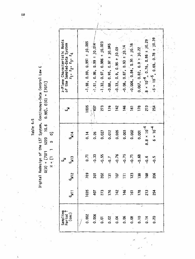
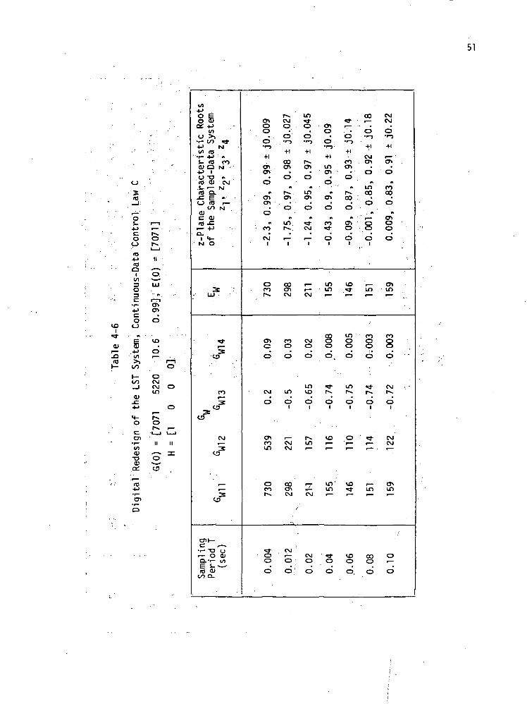
0 0] are shown in Table 4-4, and the results with control law C

for H = [1 1 0 0] and H = [1 0 0 0] are shown in Tables .

4-5 and 4-6, respectively.

The z-plane characteristic roots of the redesigned systems in

Tables 4-1 through 4-6 are shown in Figures 4-1 through 4-6, respectively.

These results show that a large variety of sampled-data systems

are avai'labl'e to control the digital 1ST. It is apparent that the

choice of H plays a very dominant role in the resulting gain GW(T).

In fact, with control law A, while one choice of H (Table 4-1 and

Figure 4-1) provides a stable sampled-data system for a wide range

44

of sampling periods T, another choice of H (Table 4-2 and Figure 4-2)

yields a system which is unstable at higher sampling periods (T greater

than 0.5 sec). Still a third choice of H (Table 4-3 and Figure 4-3)

yields a system which is stable only at very low sampling periods

(T = 0.06 sec or less). With control law C, and H = [1 1 00]

or H = [1 0 0 0], the redesigned system is unstable for very small

sampling periods (T less than 0.018 sec and 0.02 sec, respectively).

In general, it appears that control laws A and B are more effective

when digitally redesigned.

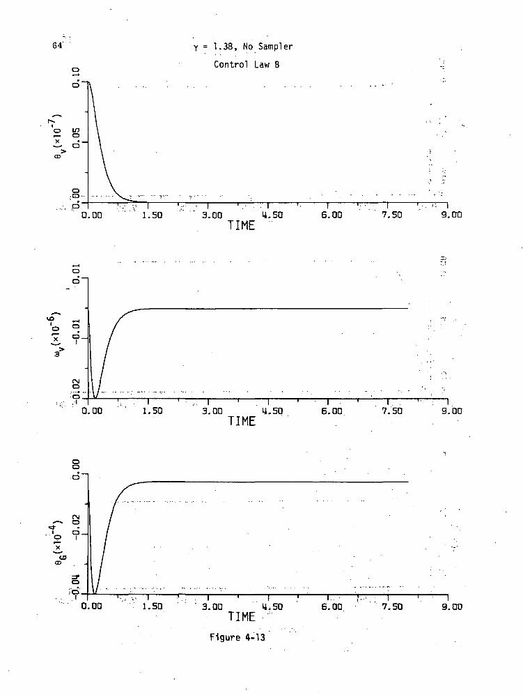
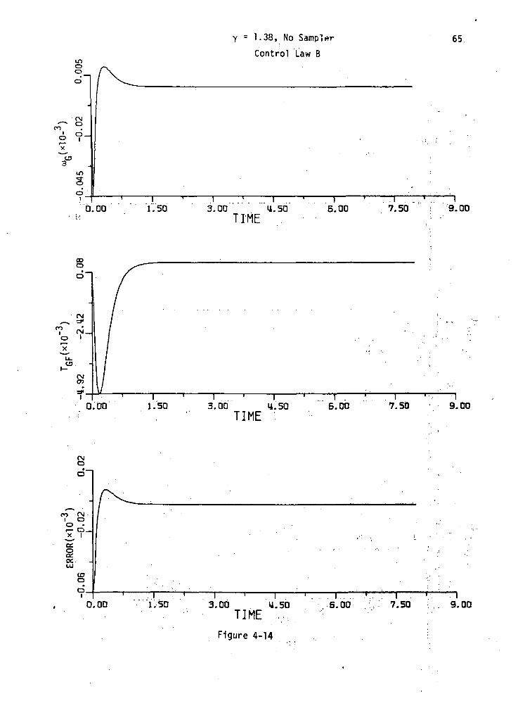
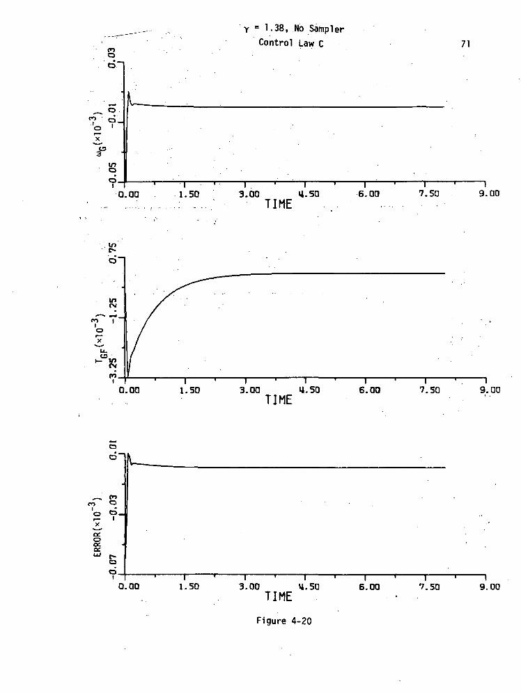
Some computer simulations are now presented to show the effects

of digital redesign with the various control laws. As before, only the

first two feedback gains are utilized, and the simplified 1ST system is

simulated on a digital computer with the CMG nonlinearity included. The

,-8parameters of the nonlinearity are y = 1-38 * 10 , TGFQ = 0.1. In all

the simulations, the input x = ° and tne initial value of 6V'(0) = 1 * 10"°,

with all other initial states equal to zero.

The following simulations have been performed:

Figure No.

4-7, 4-8

4-9, 4-10

4-11, 4-12

4-13, 4-14

4-15, 4-16

4-17, 4-18

ControlLaw

A

A

A

B

B

B

H

_

[1 1 0 0]

[ 1 1 0 0 ]

-

[ 1 1 0 0 ]

[ 1 1 0 0 ]

Sampling PeriodT (sec)

. Continuous-data System

0.02

0.1

Continuous-data System.

0.02

0.1

45

Figure No.

4-19, 4-20

4-21, 2-22

4-23, 4-24

ControlLaw

C

C

C

H

.

[1 1.0 0]

[1 1 0 0]

Sampling PeriodT (sec)

Continuous-data System

0.02

0.1

In each simulation, the following quantities are plotted:

0V = vehicle position (radians)

o>v = vehicle velocity (radians/sec)

0G = Gimbal position (radians)

o)g = Gimbal velocity (radians/sec)

T- = Nonlinearity Torque (ft-lb)

Error = x .-. KQ9V -

= Error input to CMG controller.

The simulation results show that adequate digital control schemes

can be obtained for wide ranges of sampling periods by appropriate re-

design of the feedback gains. Again, it appears that the method of

redesign is more effective in the case of control laws A and B.

46

5fO

os-

O I—I<_> 00

inIB r»4-> m

•s -I II

</>

§ s-

o o•— o

cu £I— •(-><O >>

1CO O

invV•§or

(O

•r-0>

O

<*-o1/1

4->OO

DC

(JO) **••r- 4-> N4-> V)< / > > > •

•r- IO CO

Ol «J•M 4-> "O <O CM(0 O NS- 1(0 TD «

O^N

C 1003 CO

i .cN 4J

2LU

«*

CS

CO

3 3ts e;

CM

3C3

O

0)1—

•r- -O Oi— o cu

E i •n 9)

<s> a.

«o<T> O

to co • i— r-S CO ro •— • CM O O

Or— -ocMLrtr>.a»ro 00 i '.. .• O •>-> -CMCMCM -»*-^-VO

o o o ••-> o • • • o ro O o> •••r-jT-j-r-j +l'roOOO'f> • • O ^"

+1 •«->•!-> i-j O O • VO+1 +1 -H VO -H +lTTi->OO

<* 1 +1 +1 +1 1 •10 o vo • i— - «j- +i +r cw o> oo o o r». rs vo oo. UD . _. •• »OOOO "OOO 'Or^r— «* O

^- o . . . .•> •» •» «* j- » « M •» CO CO CO CO

nma»voOi— F-CVI -CMCM CM r— r— • Ul U3 VO CO LT> • • « • « • • '

• • . -ooooinooo cxr>•»-O*r-> •(->•!-> OOO « O O O O O

+1 O r-

VOVOfÔO " ITJ -d -COCOX00 CJ» CM r- •— CM CM — r— O O O OmcMi— coooooooooooo0000000000 0 0 0 t-

00I^lf)^-OOCOOOlOCTl^J-CT>i— CT> "CMlf)«i-r— inrÛIr— <t-VOVO^-OCO^'r^ r^ r~ vo ir> .or> r— o> r^ CM in oin in in ir> in in in-tn »s- - CM • r

~r'~"'\.

- ^

i i i i i i i i i i i i i |-- — •o o o o o o o o o o o o o o

x x x x x x x x x x x x x xin vo

OOVOCOr- OCOin,— VOOCOO>^-00

r— voi— CMnco«i-ininvoincMi— r^

r-»CM^-r^cn CMro^-mincMvOMr—OOOOl— r— i— i— r- r- ,— OOO

oooooooooooooo

vooi— r«.<Ti«*(»>in^3-ooo>irôoiÔOOr— •— r— i— OOOVOrOvDVOCMCM

oor^.in**-cocoooinvT»«*cn (— en -CMin^-r-inrîn^-^j-vovOr— oconftî^r^voin^rooi— ent^CMinoLnLntnLninininLn^-^-cM i—

i— CMro**~invoiôocyi inOOOOOOOOOr-CMinOO

O O O O O O O O O O O O i — CM

47

<o

<3

O

•cO I — I0 S10 t~--i-> inro i— io

i u

o o

C I—Io o

£ OO)

to r-~CO r—

1— r-

_l

•r—

O)

o^>O £O >•i- to^_)(/> (O

*r— 4J

O) O•«-> 1 .O t>to 0)

ro CL-c EO <O

toOJc <u10 JC

i— 4J0- •

1 <*-N O

^^Nl

ft

CO .Nl

nCM

M

•t

r—N

UJ

CD

c•— oO.-r-e s-<O QJtO Q.

^^• r—3

cr>

CO

3C-5

CM

3C3 .

,_r—

0?

oOlt/1

V *•

CO

so•I-J

+1 •l«-CT)

CD

•. CO-

CM

O•<->

+1

voCM •

•'o

ootoin

|

0r— •

X

ooCM

CMr_

,O

f^.CO^*

• " 1—

ooinVOin

CMo.

o

CMCM•"•.

O•*-)

+1

CMr—

c1

. •*CM^~

•O

•••"-J

+1

VOcoCD

COCOCO

CO1of^

X

^*"r~

CMCO

o

fv.enCO1 —

COCOCO

o,

o

COCOoCD

1

n

^.oft

CMcoCD

1

flf*^CO

COr>-10co

CO1or~

X

CM

in

CM

.O

ooCM,—

1

co

oo1

<£>O.

O

CMO

•O

1

fl

coCO

CD1

ft

. \o .in

•O

«. r—

•inf—i

0

X

inCM

f^f~o

•

01

Cf>CO

•1

o

X

r~»CO

inor~X

IT)•

CM

S.

O

CM

O

O••->

+1

inCMOCD .

A

1 —"3-

CD

'*CM

•COini

ino

• X

10

"*

COo•

CD

•O

o

X

<o

^

inor~X

VO•

.

o

•48

<

«J

o+•>c .O I — Io oo

LT>03 r~»4-> inHJ I — Iai n

o o3 ---

C (—Io o

CO O

w cB

co rs.co o

QJ 00jz in

ID r-4- I—I I—Ibc i. ,iO) ^~ Z•i- O

CU IS

"8ae.

10

£o eo cD

ee. 4->i/>

o >> «*•.•i- OO N

</) fO "••.- +J CO

i- IO IMO> O4J 1 ' •O -O CMIT} CU tsl

• i. •—fO Q. •> --c E •—o 10 N

00cuC CD

f~~ 4-JQ. .

1 V|_M O

3LU

. ;-:..cs

ro

3 C?O

CM

IS .

i—^g •

•r- "O Ui— O 0)

J JL ••••• 'CUO.

cnOOoCD•1—5

•H

)

CM•

0

** -CM

O

+1

CT*CM

•

O

inin

ini

.. 0

X

«*

"*

COoCD*

oVf>

'f^

CM

C3

oooCD

*•»->

+1

coinO•O

v>f*s.

•—CD

+1

r— .

00

CD

Oj ^in

iO

X

^>

•~

fx«oCD

H-'.

•*

sID

sC3

inCM

" COo

•o

1ft

r—m

O

r.

CM•

O>rO

+1

f^•

CD

cninin

i0

X

VO

CM

VOCT>O

0

VO

*!•

,S? .IDID

voO

0

p-

oo

1

^COr—..

0

•tCDCM.

CD•1—5

+1

VO•

O

OvCM^fin

iO

' X

f^CO

oo

CD

5<•

CM

^^

§CD

^OCOooo

•t

COI—

•o

•t

COCO

CD•f— 5

+1

in•

O

CO

CMin

"70

X

vo

*

COr—

CD

K

CO

CO

CMID

O

O

C•

o#>

ss•

o. f

CMCO

CD•1—3 '

+1

^^r«

•O

ooCOCOCO

1o

X

cqm

CO

CD

o. «—

. . -

CO

IDCM

C3

O

CD

•«VOoo

•o

•t^>fs .

oo

1

*l!__

O•

r^

COCO^J-

10

X

r-.

"*

en 'oCD

r— ' .O

3

0ID.

0

O.

o•

«^CMOO

CD1

*inin

8.

Oi

M

r_ ••

f__ ,i

COinCO

io

X

.-CM

VO

O

CD

OIDCO

COIDPO

Opj

O

CD

•i

inior—x

^~•

CM

^ "|

O

X

toCM

1

M^^>'o

. •^_

1

CM

inoo

i0

X

0

•~

,CM. O

O

r^:. . • .

CM

ID00

pCM

49

os- i— i

4-> COC 1^o r-»o mRJ

•>-><oQV)

o

II

C?

•1- •*-l-> Oo o

QJ10>>

GO

O)

o>O

CM

S oCM

co<«- r-.O r-

in i—C I—I I—Iw II•r- II(/IO) *^

•g s

O)•^O

in4JO EO Q)ry 4.1

in0 >>

4-> tslin <o

i- <o coco o No -o •<o a) CMS. r- N

-c E •>O <O i —1 CO MQ)C 

' -H

CMcn

d. ff—CO

•

o

*in.

0

COCM

VO

§0

d

CM

d

e»r*.

COCMCM

«M

O

« -

r—

0•1—5

+|

^>00

c>#»

o>VD

•o

*l

CO

di

CMCMCO

. ^COood

COCO

di

voVOVO

CMCMCO

S*o

CMCM

O•i—)

+1

VOr^d*

^^VO•

oft

8di

oco

CMo0

d

r—CO

di

s»

o00

VOoo

enCM.o

+1

en .vo•o.

^_

VO

dfi

ooCO0odi

COCMco

CM

.0od

VOCM

di

CO

VO

COCMCO

8o

inCO

o•f— y

+1

COVO

d'*

f**^

. in•o

A

gO

d

CM

CO

io•~X

cr>

CM

di

0co

CM

CO

O

o

r**j-.

0

!•*•!in

d

N.• •

' O•i

^1O

X

co

%CO

T'o

X

CO

VO

co0

di

^r*.

c^CO

•

p

s.

0

COCO

dr,

CO••

oft

ini0,_•

X

ini

r_

r^

iO*~X

a>

**

io

X

§

rxf»

oCM

• o

50

ini

flj

3

Sas

OJ- i— i

o oo r>.

i — ito•u n10o *— *I O

V> — '3 LUO3 •C I— I•i- VT>

o o

VO

•M O(/> ' i—

(- OOO CM_l CM O

in

0 ors. i—C I I I—Ien••- ii iti/>co -— oc^g S01 CD

<e4->•I—en•i—o

IO+J

O COOC 4->

VI0 >>

•w- CO4-)u> to•r- 4Ji~ roai a+j io -oro wi. r-co a.jc e

C_) fOCO

VC rtlw«3 S.

i— 4->o_1 4-N O

i T*

^vCD

Cnh-

•p- -ar- O

g-ri«co a.

<*N

9t

CON

»CM

N

•k

Nl

E '

*1-

•»C3

CO

5o

CM

•»o3

rgts

Ocuin

ino0

CD•'-}

+1

r—a>cn

• '

0

«t

cnen

CD

COin,_!i

in0

«*

CD

r^CD

cnvo^^

inCOQ

CM0

. . O

/ o//

/j

i1

4*-0

CD••-J

+1

<3\• cn

«

0

ft

cocnCD

in,_!

'

; rs.

r§r1 \

inoCD

COCO

CD

oCO

rs.O^-

VD0O

0

COCMoCD•i->

+1

VOCOenCD

»rs.enCD

CMCO

,_!

COrs.CM

r-CMo0*

ininCD

CMoCM

COrs.CSJ

0

CD

in5CD•"-)

+1

rs.cnCD

»If)Cn

o

CO00

CD1

voIS.

CM

oCD

IS.

CD1

r~CO

VOIS.

CMO

CD

cn0

CD•f-)

+1

incn

o- *cn

CD

COCO

CD

CM*fr

inooCD

VOrs.

CD

5

CM*r

cSCD

•^• .'O•r

+1

.COcn

.CD

• •>>s,00

CD

4o

1

VO^1- .

ro8CD

inrs.

CD1

-

VO^~

voO

CD

CO

CD••n

-l-ipM

.cn

CD

• *

«S-CO

•k*3"ooCD

1

VO

CM0O

CD

PI

O

COCM

VO

§

CD

CMCM. •O•<->

+1o»CD

fi •CM00 '

CD •

rs.g\~J

CD

COts.

0oCD

CD1

%

COrs.

o

CD

cnCM

CD•i >+iVOooCD

M

VOrs.

CD

*."1CD

X

.00

CO

CVJ

(J-o

00

00

VO

o

%

CO

^^

^J-

CD

cn .CO

oT>

-noo. rs.CD

m

cnvoCD

*if)1

. o

X

in

• •**,in(VIv^

«ti-io

VO

inCDi

vooCNJ

^tin*viv^

oCM

CD

51

10

o•>->oo

oI

10

n

o.

10I

0.n<tJ

•r- cn+j cno

<_>

in>»to

10

CD

oCMCM Oin

O)•1- IIincu *-*-o oCU -Q; o

CT)•r^a

I/I

O Eo 35ct -t->

VIu >>•r- tO «3"•4-> NI/I (O

' •!•• 4-* «»$- (O COCD O N

+-> 1

(t) CU CMS- >— N(t) O.

-C E « • .-O «3 r—

00 NCUC CU

i— 4JQ.

1 4-N O

LU

^yj

CO

3

CMr- '

^_

3CJ3

0>1—

•r- T3 Or- O CUQ.T- (/)p J_ .

n) cuOO Q.

^0o0•r-J

+1

cnencb'

»a*o>

^3

**• CO

•

CM

oCO

C

O

CM

O

cnCOin

0COr-

• oo.

o

CMO .

j^ ••i-}

+1

oocn•o- «^«^cn .• •o*

in•

P_

ooCM

COO

O

inCD

t

CMCM

oocnCM

/

CvJ

O. •

O '

in^0

CD•*->

-f 1

^^cn•o

«incn.o

A

CM•

r—

CM

CMO

CD

in10CD1

^'in

f^C\J

CMO.

O

cnod•T

•H

incnCD

9>

0^•

O

«CO

•

o

in• in

00

§

. °-

r~«CD

1

IO•—

in'in~

o.o

^^r—1 •

O••-J

+1COcn• •o

*p^ooCD

««cno

•

oi

10

inooo

int^CD

'

O'•—

IO^>r—

O

CD,

oo•

o

+1

CMcn•o

•tincoO. *

• ' f—

8•

o

in

' COCoCD

r~-

CDi

•—

r-"in

§CD

CMCM

•0

+1r— •cn•o

•t

COooo

»cn0o

•

o

in

COooQ

CMr>»o1 .CMCM

cninf—

o.

o

55

•M O

56..

CO

>>CO

co

O)

O- o

CO

•»JOO «—

CO••- IIL.

O •to (_>

«s 5-C (O(J _l<U i—C O<o s.i— -MQ. CI O

IM O

ini

s-3ov

58

= 1.38, No Sampler Control Law A

0.00 1.50 3.00 4.50 6.00 7.50 9.00TIME

0.00I ^ I ' I ' I ' I ' I

1.50 3.00 4.50 6.00 7.50 9.00TIME

1.00^ i ' n ' i r1 i ' i

1.50 3.00 U.50 6.00 7.50 9.00TIME

Figure 4-7

0.00

= 1.38, No Sampler Control Law A59

I ' i^ ^v I ' . i . • .1 i1.50 3.00 U.50 6.00 7.50 9.00

.TIME

0.00I ' I I I 1 I

1.50 3.00 4.50 6.00 7.50 9.00TIME

0.00i ' r ' i * i ' i ' i

1.50 3.00 U.50 6.00 7.50 9.00TIME

Figure 4-8 \

60

= 1.38, T = 0.02 sec

Control Law A

I ' I ' I ' I ' I \" I0.00 1.50 3.00 H.50 6.00 7.50 \ 9.00

TIME V

Q.OOi : • i • i • i ~ i ' i

1.50 3.00 4.50 6.00 7.50 9.00TIME

Q.OOi ' i ^ i ^ T^ • n • i

1.50 3.00 U.5Q 6.00 7,50 9.00TIME

Figure 4-9

61

0.00

Y = 1.38. T = 0.02 sec

Control Law A

, 1 | . | 1 | I , I ,

1.50 3.00 11.50 6.00 7.50 9.00TIME

Q.DO1 ' 1 ' \ ' ! ' \ ' 11.50 3.00 U.50 6.00 7.50 9.00

TIME

.8<=n

o.oo 1.50 3.00 U.50 6.00 7.50 9.00TIME

Figure 4-10

62

a>o

'o g^ CD'

0.00

Y = 1.38, T = 0.1 sec

Control Law A

o1

^^ . - '; •':I • I • i i , • i • , i

1.50 3.00TIME

6.00 7.50 9.00

,. o.oo

VD

O

X

>

s•

o_1

(nooiy i • i • i • • i • i ,

0.00r ' i ' i ' i ' i ' i

1.50 , 3.00, U.50 6.00 7.50 9.00TIME

Figure 4-11

63y = 1.38, T = 0.1 sec

Control Law A

o-r0.

1 .DO

l1.

•50

i3.00

'

TIME

iu.

•50

1 '6.00

I7.50

. . . |9.00

0.00I ^ 1 ' I

1.50 3.00 U.50TIME

6.00 7.50 9.00

0.00 1.50 3.00 U.50 6.00 7.50 9.00TIME

Figure 4-12

64

o'«—i•„

O

Y = 1.38, No Sampler

Control Law B

r-.'o \r>•— o

~> d~<D

Orr\ .• \^J •*

, o0

0

"1«o" -,° ^i ?-3"

OJoo

; • • • . - . ,:l0

o0

• —

.(M

•f °.T° f~

X

*~ta(D

0

To• .. ..i

0

I

\ : ..X -x^_ ! 1 : • ' •

.'.,- "'1 ' •• • ' 1 ' - . 1 '• 1 ' - 1 ' ' '• . >-- 1

.00 "" 1.50 '" " 3.00 U.50 6.00 " 7.50 ' 9.00TIME

•'-':

1 f// :'/ ; : • ?

\y :

': 1 ' , 1 ' 1 1 ' 1 ' : 1

.00 1.50 3.00 U.50 6.00 7.50 9.00TIME

.

1 / ;

// ' ' " " • '

/\\ j . . . - - • , . • .

' , v 1 • ' . . 1 ' 1 ' 1 ,'.-• 1 ' 1

.00 1.50 ' 3.00 U.50 6.00 ' 7.50 9.00TIME

Figure 4-13

0.00

Y = 1.38, No Sampler

Control Law B

65.

Y.50 3.00 U.50TIME .

6.00 7.50 9.00

o.dol ' I ' \ ' \ ' . \ ' I

1.50 3.00 U.50 6.00 7.50 9.00TIME

0.00I ' 1 n I

1.50 3.00 U.50TIME . . . .

i \^. i ~ T n6.00 7.50 • , 9.00

Figure 4-14

66

o• „

o

o gA CD'

o•

o.

Y = 1.38, T = 0.02 sec Control Law B

0.00 1.50 3.00 14.50 6.00 7.50 9.00TIME

0.00I ' I ' I • I ^ \ ' I

1.50 3.00 U.50 6.00 7.50 9.00T I M E

0.00 1.50 3.00 U.50 6.00 7.50 9.00TIME

Figure 4-15

67

<£>

O —|

O

CVJ•—* o

co: oio o

3°

rsio

y = 1.38, T = 0.02 sec Control Law B

1 'I i - I • f • | ... -r 1 • . I

0.00 . . . . .1.50- 3.00 -U.50 6.00. ,:.:>•_- 7.50 • -, '-.. 9.00,v.i - ' n::\ , J I M E . , v ' -. ' . -.

CD

i n0.00

i * i ' i i i • r ^ i1.50 3.00 U.50.. ,. - 6.00 , - 7.50 . 9.00

-;: ^ T I M E

oo"

i oo

OLoCSL

(MO

O.I i I ' I ' I ' \ ' l.0.00.. ^ ..._ 1.50.. ..3.00... U.50 . 6.00 7.50 9.00

• : T J M E

Figure 4-16

68

•Q.QC

Y = 1.38, T = 0.1 sec

Control Law B

1.5D . 3.00 U.50TIME ,

6.00 7.50 9.00

0.00 1.50 3.00 U.50 6.00 7.50 >. 9.00TIME

0.00

1 I ^ T 1 I ^ T n I1.50 3.00 U.50 6.00 .7.50 9.00

TIME

Figure 4-17

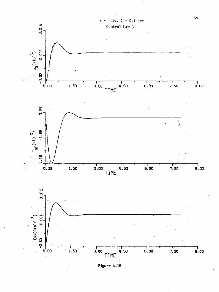
1.38, T = 0.1 sec

Control Law B

69

0.00 1.50 3.00 «.50 6.00 7.50 9.00T I M E

O.OQ 1.50 3.00 4.50 6.00 7.50 9.00TIME

0.00 1.50 3.00 U.50 6.00 7.50 9.00TIME

Figure 4-18

70

1.50

= 1.38, No Sampler

Control Law C

3.00 U.50TIME

6.00 7.50 9.00

od'

0-1X I

\f>

o.

0.00 1.50 3.00 H.50 6.00 7.50 9.00TIME

inoo-.

X I

3°

inCMoo-i

0.00 1.50 3.00 U.50 6.00T-IME- ;

7.50 9.00

Figure 4-19

too

<

inoo.i0.00

Y = 1.38, No SamplerControl Law C 71

1.50 3.00 U.50 6.00 7.50 9.00•: TIME

0.00I ' T T I 1 I ' I , 1

1.50 3.00 U.50 6.00 7.50 9.00TIME '

oCD-

CDr—X

Of.

§

O.

0.00I ' I ' T ' I ' I ' I

1.50 3.00 U.50 6.00 7.50 9.00TIME

Figure 4-20

72

r>

5-

0.00 ;' l.SO

y =.1.38, T = 0.02 sec

Control Law C

3.00 ; u.sdTIME

6.00 7.50 " 9.00

Q.OQ

in ''o

0.00 • 1.50 '•• 3.00 r U.50 6;00 7.50 9.00TIME

Figure4-21

oo

o _

(MO

0.00

1.38, T = 0.02 sec

Control Law C73

1.50 3.00 U.SO : 6.00 , 7.50" 9.00T I M E : ;

o(O

0.00 1.50 , 3.00 U.SOTIME;:

6.00" 7.50- - 9.00

o-,o

sd.

0.00 1.50 3.00 U.50 : 6.00 7.50- 9.00TIME : - ' .

Figure 4r22

74=1.38, T = 0.1 sec Control.Law C

o o

sO.

0.00T ~ F • I • T "^ I "^ I

1.50 3.00 ii.50 6.00 7.50 9.00TIME / :

0.00

3.00 U.50TIME

9.00

Figure 4-23

Y = 1.38, T = 0.1 sec Control Law C 75

0.00 7.50 9.00

! T - - i i i i - - ^ i - ^ i • - j i j

0.00 1.50 3.00 U.50 6.00 7.50 9.00TIME

CM0_

ox

8o_<!Lzi

0.00 1.50 3.00 U.50TIME

6.00 7.50 9.00

Figure 4-24

76

5. Stability Considerations and Constraints on the Selection of theWeighting Matrix of the Digital Redesign Technique

It has been reported [6] that given a continuous-data system

x(t) = [A - BG(0)]x(t) (5-1)

the solution of the feedback matrix G(T) of an equivalent digital

system, designed with the point-by-point state comparison method,

must satisfy the following equation:

e(T)6(T) = eAT - eC- (5-2)

Since 0(T) is usually not square, we cannot solve for G(T) directly from

the last equation. One remedy to the problem is to introduce a weighting

matrix H, such that the inverse of H0(T) exists. Then,

GW(T) = [H6(T)]-1H[eAT - e ] (5-3)

However, the weighting matrix H cannot be chosen arbitrarily. The

solution in Eq. (5-3) is significant only if the digitally redesigned ; /,/>

system is stable. . ,

In chapter 4, it has been demonstrated in the digital redesign.

of the 1ST system that for some sampling period T and some H, the

resultant GW(T) gives rise to an unstable closed-loop digital system.

This means that given the continuous-data control system, the weighting

matrix H cannot by chosen arbitrarily. The conclusion is that if the

closed-loop digital system is unstable, the solution to GW(T), corresponding

to the selected H, will be meaningless.

77

The problem now is to find the condition under which an H can

be found such that the digital system is stable.

Stability of the Closed-Loop Digital System

The state equations of the digital system are written

1)T] = 4>(T)x.(kT) + 9(T)u(kT) (5-4)

where

eA-T (5-5)

9(T) = eAXdAB ,(5-6)

The feedback control is

u(kT) = -G(T)4(kT) , . . . , . . (5-7)

Then, Eq. (5-4) becomes

" DT] = [<fr(T) - e(T)6(T)]x(kT) (5-8)

The digital system is stable if all the eigenvalues of [4>(T) - Q(T)G(T)]

are located inside the unit circle |z| = 1. Since <fi(T)'and 9(T) are

known once the sampling period T is specified, the conditions on G(T)

for stability can be established using well-established techniques.

L e t . . - - • - • ' • • • - . , . • • .

eAT . e[A-BG(0)]T ; D(T) ' (5.9)

and premultiplying both sides of Eq. (5-2) by the 1 x n matrix H,

we have vc . •'

78 . .

He(T)Gw(T) = HD(T) (5-10)

where G(T) has been replaced by G,.(T) to,indicate the !• weighed ttiatc'hirig

of states. i v

Taking the" matrix tr^frsppse^y6ri^}^

w e get, • . . , . ' . ; • • •

1 = D ' (T)H ' (5-11)I • • • • . . • • ' • ' ' • ' • • ' . . -

Rearranging, Eq. (5-11) becomes , - ,

- D'(f) ]H' = 0 (5-12)

This equation represents a set of n linear homogeneous equations which

have nontrival solutions if and only if the following condition is

satisfied: - - - ___ ____

[I) - D ' (T) | • 0 (5-13)•'- ' / " ' '

/ which^is also equivalent to • . ~"

/ |e(T)Gw (T) , - D(T) | =0 ' ' . (5-14)

' / : . ' . . -

/ Thus, if Eq. (5-14) is satisfied, there is/ always a nonzero H which

/ will satisfy /

'i--1 • . : • ' = . - . • • : . . • / - . • . -. •. ••G (T) = [He(T)]"1HD(T)/ / (5-15)

. • « > ' - • - • , /

Illustrative Example

Consider the continuous-data system •'/

x(t) -'Ax(t) : ,t Bu(t-)

79

(5-16)

where

A =0 1

0 0B T'-

0

T

G(0) = [2 3]

It is desired to design a digital system which will match the response

of the continuous-data system at the sampling instants. The sampling

period is 1 second.

The following.matrices are computed: t

4>(T) =

6(T) =

D(T) =

1 T '

0 1

0.5 '

1

1 1

0 1

0.767 1.233

0.465 1.097

The characteristic equation of the closed-loop system is

2F(z) = 6GW(T)| = z + [-2 + O.SG^T) + G2(T)]z

+ [1 - O.SG^T) - G2(T) + TG^T)] = 0

(5-18)

where G^T) and G2(T) are the elements of G (T); that is,

80

G2(T)] (5-19)

Using the Schur-Cohen stability criterion, the roots of Eql (5-18)

are all inside the unit circle if

. ' . - . • • ' ! '• - '• ' V:F(0) = 1 + 0.5^(1) - G2(T) < 1 . . . . . . .;.,_, (5-20)

F(l) = '6^1) > 0 . " ' (5-21)

F ( - l ) = 4 - 2G2(T) > 0 (5-22)

These conditions on G,(T) and G2(T) are plotted in the parameter

plane of G2(T) versus G^T), as shown in Fig; 5-1. •••:

Having established the conditions.on the elements of GW(T) for the

stability of the digital system, we turn to the condition under which

an H exists which also satisfies Eq. (5-15).

Equation (5-14) leads to .

|6(T)GW(T) - D(T)| =

0.56^7) - 0.767 O.'SG^t) - 1.233

G^T) - 0.465 G2(T) - 1.097= 0

(5-23)

or

-0.535G2(T) + + 0.268 = 0 (5-24)

Equation (5-24) represents a straight line in the GgtT) versus

G^(T) parameter plane. The intersect between the line represent

by Eq. (.5-24) and the ;stable region gives the stable trajectory for

•6j'(T) and,G2(T), as shown in Fig. 5-1.

81

If the intersect between Eq. (5-24) and the stability region of

G,(T) and $_(T) is convex } n general , the vertices ,of the intersect

can be used to find the, bounds. on the weighting matrix H. -

In the present Case, the vertices .of G,(T) and G?(T) are at

(0, 0.5023) and (1.171, 2).

Substituting the vertices of .6 (1) and G2(T) in Eq. (5-12),

we have the two boundary equations for the elements of H = [h, h ].

G^T) = 0, h1 = -0.606h2 (5-25)

6^1) = 1.171 h1 = 3.875h2 . (5-26)

Figure 5-2 shows the region in which h, and h« should lie so that

Eq.1 (5-3) .will always yield a state,.feedback control such that, the

digital system is stable^ -

82

o4->3

"o

<o>

o

uo

O

0)s_o>

I •in

83

S-o

•o03

co

(O

o

OJs_

8,4 .

6. Realization"of;1 State Feedback liy EiynaitiiG'iCpntrol ers';; .

One of the unique ehara'c'teristics of'modern control theory .is'that

optimal control is often realized by state 'feedback. For instance, It is

well known that if a system is completely controllable, its eigenvalues

can be arbitrarily assigned through state feedback, and the optimal

linear regulator design always leads to a state feedback solution. Un-

fortunately, in practice, not all the state variables of a physical

system are accessible. Considerable amount of results have been reported

in the past on the design of optimal systems with partial state feedback.

The basis of the classical control system design_ijs'that the

configuration of the controller is selected a priori. The controller

used in practical systems usually assume the form of cascade or feed-

back controllers, or a combination of these. In these cases, only the

outputs of the system are fed back. One advantage of the classical

controllers is that they can be implemented often by passive filters or

electronic circuits.

In this, chapter we shall present a method whereby a system with

state feedback is approximated by a system with a cascade controller.

How the state feedback is determined is immaterial fbr the present

analysis; it!can be obtained from the pole-location solution or the

Riccati equation solution, or some other optimal control design methods.

Continuous-Data Systems

Consider the system •' .

x(.t) = Ax.(t) + Bu(t)

.('t) = Cx(t,j •+ Du(t)

85

(6-1)

where

x_(t) = n x I; state vector

ujt) = r x 1 input vector

- in x l output vector

A, B, C, and D are coefficient matrices of appropriate dimensions^.

Assume that state feedback is given such that : .

u(t)K-Gx(t)' •-• . • . , . ' • • (6_3)

where G is an r x n feedback gain matrix.\ •

\ The design objective is to approximate the system of Fig. 6-la\ , • • , - . . • ' • • " . " . " • " .

which is described by Eqs. (6-1), (6-2), and (6-3), by the system of

Ffg. 6-lb which has a feedback controller with feedback from the out-

put Variables. Let the transfer relation of the controller be repre-

sented xby

U(s)\-H(s)Y(s) • • • • • (6-4)

where H(s) is the controller transfer function matrix:\ . '

. . ... Hlm(s)

H21(s) H22(s) ... H^s)H(s) = (6-5)

Hr2(s)

86

Let H. . (s ) (i =' 1, 2, ..., r; j = 1, 2, ...., m) be a pth order* J .

transfer function, - - . . . . . .

„ ()1J •"•

The transfer function H.-(s) is expanded into a Taylor series

about s = 0,

where

(6-6)

s =. 0(6-8)

Evaluating the coefficients of .the Taylor series, we have

"ijo •

and for k > 1,

k-1..' ; dijk = aijk ' Bijk - (6-9)

Since the state feedback represents the feedback of the system

output and its higher-order derivatives, a truncated series expansion

of H.J.J(S) may be used as a dynamic implementation of state feedback by• J

87

feeding back only the output variables.

If the infinite series of (6-7) converges, we may approximate it

truncating it after p terms,.where p is hot.yet specified. Let us

introduce the. notation, H.. (s), for the truncated version of H...(s);

then

(6-10)

where d.. k is as defined in Eqs. (6-9).

Substituting Eq. (6-10) in Eq. (6-4) for the elements of H(s),

we have

U(s)

ill

211

Kr1[drlO.

K12Cd12120

K22Cd220 d221 '" d22(p-l)]

dr21 -

lml

2nl

nnl

•(6-11)

88

The elements of the last equation are rearranged to give

f'Klld110 K12d120 •'• VWCKlldm K12d121 •" Klmdlml] •" fK11dn(p-l) *12d12(p-1) •" Klmdlm(p-1)]

[IC21d2lO K22d220 *22d221 [IC21d21(P-U K22d22(p-l)

U(s)

Kr2dr21 " "' rldrl(H) }KrZdr2(p-1)

The time-domain equ'ivalence\ of the last equation is

u(t) = -F

where F denotes the r x mp coefficient matrix in Eq. (6-12).

From Eq. (6-2),

= Cx(t) + Du(t) .

= (C - DG)x(t) :

(6-12)

(6-13)

(6-14)

Then,

89

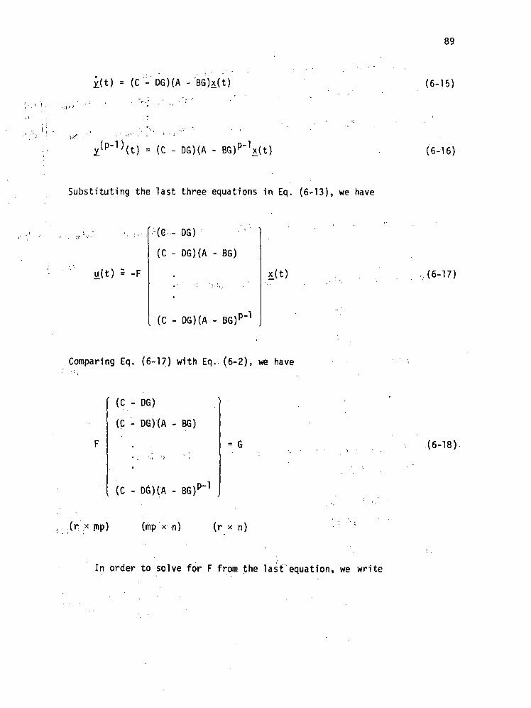
i(t) = (C - DG)(A -'BG)x(t) (6-15)

= (C - DG)(A - (6-16)

Substituting the last three equations in Eq. (6-13), we have

u(t) = -F

•(G -DG)

(C - DG)(A - BG)

(C - 06) (A - BG)13"1

x(t) (6-17)

Comparing Eq. (6-17) with Eq. (6-2), we have

(C - DG)

(C - DG)(A - BG)

= G

p-1(C - DG)(A - BG)

(r ,x jnp) (mp > n) (r x n)

(6-18)

In order to solve for F from the last equation, we write

90

F = G

(C - DG)

(C - DG)(A - BG)

(C - DG)(A - BG)P']

-1

(6-19)

if mp = n, or p = n/m. This means that if n/m is an integer, we may

truncate the Taylor series expansions of 6 (5), ;i<- U 2, -.-.,.;, r,

j = 1, 2, ..., m, at p = n/m terms. If n/m is not ari; integer, we may

choose p to be an integer which satisfies

< p <m K m (6-20)

Since F is r x mp, there will be (r)(m)(p) unknowns. However, there

are only rn equations in Eq. (6-18). Thus, r(mp - n) of the elements

of F may be assigned arbitrarily.

The solution of F from Eq. (6-19) also depends on the existence of

the inverse in the equation.'

It should be noted that solution of the elements of F gives only

the values of the coefficients in Eq. (6-7). The coefficients of the

transfer function of (6-6) still have to be determined using Eq. (6-9)!*

In general, there are more unknowns than equations in Eq. (6-9). This

simply means that in the ideal situation we simply set

dijp *

and all 3.-k = 0, for k = 1, 2, ..., m. However, for a physically

91

realizable transfer function, H.-. (s) must not have mor/e zeros than1 J r

poles. Therefore, the values of g... should be assigned such that

the dynamic behavior of the overall system is not appreciably affected

by the presence of (5... , k = 1, 2, ..., m. This is similar to the

classical design practice of designing the zeros of H.. (s) to control"

the dynamic behavior of the system, while placing the poles of H.. (s)' J r

so that, they do_not have appreciable effects on the system performance.

Single-Variable Continuous-Data Systems

When the control u(tj is a scalar, u(t) = -Gxjt), where

G = [g] g2 . . . gn] . ' i (6-21)

Eq. (6-6) becomes

K(l + a,s + a,s2 + ... + a sn)H(s) = L- ^ : : 2_ ' (6-22)

Then,

H(s) = K(l + d^ + d2s2 + ... + dn_1s

n"1) . ' . (6-23)

where . . . . . . .

6k-vdv ' . : (6'24)

/'/for k = 1, 2, ..., n-1.

Equation (6-19) becomes

92

F = = G

C - DG

(C - DG)(A - BG)

(C - DG)(A - BG)n-1

• (6-25)

Single-Variable Continuous-Data Systems in Phase-Variable Canonical Form

If the system to be controlled is in the phase-variable canonical

form, then

A =

B =

0

0

0

~an

0

0

1

1 0 ... 0

0 1 ... 0

0 0 ... 1

"Vl ~an-2 ' ' ' ~al ,

(6-26)

(6-27)

and the output equation if characterized by D = Q, and

C = [1 0 0 0] (6-28)

the formulation given in the preceding section is further simplified.

Since D^ = 0, and CBG = 0, ' ' :

C - DG

(C - D6)(A - BG)

(C - D6)(A - BG)n-1

Then, Eq. (6-25) becomes

F = K[l

and

= g.

92 ... gn]

93

c

CA

CA"'1

= I (identity matrix) (6-29)

= G

(6-30)

(6-31)

ak =k-1

3k + J/k-vVl

k .= 1, 2, ...., n. , • .

Equivalent Cascade Controller

The development carried out in the preceding sections is based on':i.'' • •

a controller being placed in the feedback path of the system as shown

in Fig. 5-1b. When the reference input r(t) is zero, that is, when the

system is a regulator, it does not matter whether the controller H(s)

is in the forward path or the feedback path. However, when the input

94

is not zero, it may be desirable to determine an equivalent system which

has the controller in the forward path of the system as shown in Fig. 5-2.

In the following, single-variable notation is used for simplicity. The

problem is t'b find the transfer function of the cascade control!ler'Gr(s)**

so that the closed-loop transfer functions of the two systems with feed-

back controller and the forward-path controller are identical. The

solution o f Gr(s) is . : . . * • • : . '

GC(s) " 1 +1

6(s)[H(s) - (6-32)

where

G(s) = C(sl - D = 0 (6-33)

In general, given G(s), and having determined H(s), the order of

G_(s) will usually be higher than that of H(s).

The following example will illustrate the design method outlined

in the preceding sections.

Example 6-1

Consider that the dynamic equations of a linear time-invariant

system are given by

_x(t) = Ax(t) + Bu(t.) . . . . • - • • . . - . - .

y(t) = Cx( t ) : • • • • ' • ' . • - . ' • • • - • • • " : "

where

A =

(6-34)

0 1 0

0 0 1

0 0 - 1

B =

0

0

1

95

C = [ 1 0 0 ]

Since the system is completely controllable, we may assign the

eigenvalues of.the system arbitrarily. Furthermore, the state equations

are already in phase-variable canonical form. With state feedback,

u = -6x> the closed-loop transfer function of the system is

if- ,,-x(6-35)(g

The characteristic equation is

s3 + (g '+ Ds2 + gs '• + 9 = 0 (6-36)

Let us assume that we wish to place the eigenvalues of the closed-

loop system at s = -10, -1 t Jl» and -1 - jl. Then, Eq. (5-36) gives

g} = 20, g2 = 22, g3 = 11

or

6 = [20 22 11] (6-37)

Now consider that the states x2 and x- are not directly accessible,

and it is desired to approximate the state-feedback solution by a

feedback controller and output feedback. Since the system is of the

third order, n = 3, the dynamic controller may be of the second order;

that is,

1 + a,s + a9sH(s) = K • ^ (6-38)

1 + S^ + B2s

96

In the present case, the results of Eq. (6-30) may be used.

Thus* ~

K = g1 .= 20 ';

Oo =

Assuming that physical circuit elements allow the selection of

B, and Bo to be relatively small as compared with the resulting values

of a, and ou, we let 0, =0.15 and B- = 0.005. Then,

o^ =1.25

a2 = 0.72

The transfer function of the feedback controller is

2H(s) = 2880 S + 1'736s + ]- (6-39)

s + 30s + 200

The closed-loop transfer function of the system with the cascade

controller is

Y(s) . 2880(s2 + 1.736s + 1.389)~~ T ? ' ~"^ ~

+ 230sJ + 3080s + 5000s + 4000

A comparison of the step responses of the system with state

feedback and the system with the feedback controller is shown .in

Fig. 6-3.

.97

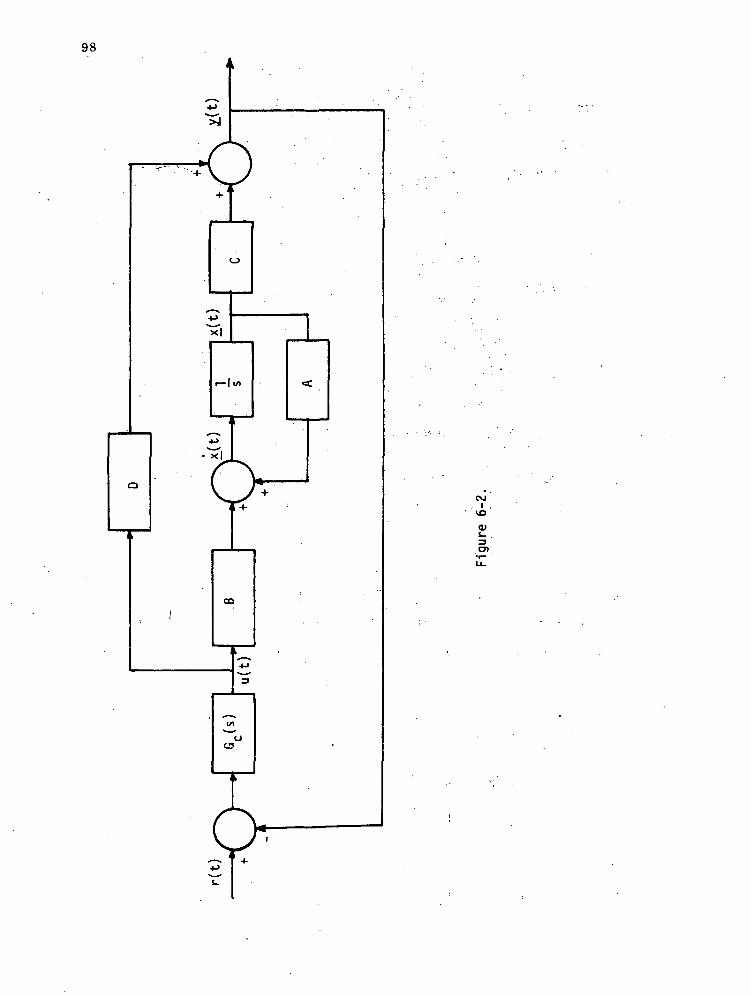
u(t) x(t) x(t) -XD-y(t)

Figure 6-la. Block diagram of system with state feedback.

Figure 6-lb. Block diagram of system with cascade controllerfrom output feedback. ; , .

98

O

x|

XUL(>CO

CVI, I .

<u'

99

Discrete-Data Systems

The dynamic controller design technique described in the last

section can be applied to discrete-data systems. Consider the dynamic

equations, ;

x(k +1) =, Ax_(k) + Bu.(k) ;

y_(k) = Cx^(k) + Dju(k)

where .

xjk) = n x 1 state vector

ujk) = r x 1 input vector

yjk) = m x 1 output vector

A, B, C, and D are coefficient matrices of appropriate dimensions.

Assume that the state feedback is used such that

ujk) = -Gx/k)

where G is an r x n feedback gain matrix.

Let the controller be modeled as a feedback controller with the

transfer function relation,

U(z) = -H(z)Y(z)

where H(z) is given by

H^z) ' H10(z) . . . Hlm(z)

(6-41)

(6-42)

(6-43)

(6-44)

H(z) =

n

H21(z)

HH(z)

]2

(6-45)

100

Let H.-(z)' be 'a' pth-order transfer function,I J

u.-

- 1J~ ... +ailD)1JP (6-46)

•Let us expand H.^Cz) into a Laurent's series about z = 0,

-k(6-47)

where

k-1dijk = aijk " 6 "

(6-48)

Truncating H.(z) at p terms, we have

(6-49)

Similar to the development in Eqs. (6-11) and (6-12), the time-

domain correspondence of Eq. (6-44) is

u(k) = -F- 1)

(6-50)

101

where F is identical to the r x mp coefficient matrix defined in

Eqs. (6-12) and (6-13), except with its elements correspond to the

coefficients of Eq. (6-46).

From Eqs. (6-42) and (6-43),

= (C - DG)x(k) (6-51)

Thus,

£(k - 1) « (C - 06)x.(k - 1) (6-52)

Also,

Ax_(k - 1) = x.(k) - Bu.(k - 1)

= x(k) - BGx.(k - 1) (6-53)

Therefore, '

x(k - 1) = (A - BG)"\(k) . (6-54.)

Substitution of Eq. (6-54) in Eq. (6-52), we have

- 1) = (C - DG)(A - BG)"\Ck) (6-55)

Similarly,

- 2) =(C - DG)(A - BG)"2x(k) (6-56)

- p + 1) = (C - DG)(A - BG)"p+1x.(k) (6-57)

Thus, Eq. (6-50) becomes

102

Li(k) * -F

C - DG

(C - D6)(A - BG)-1

(C - DG)(A - BG)'1*1

x(k)

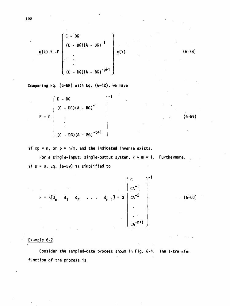
Comparing Eq. (6-58) with Eq. (6-42), we have

C - DG ^"]

(C - DG)(A - BG)"1

F = G

(C - DG)(A - BG)"P+1

(6-58)

(6-59)

if mp = n, or p = n/m, and the indicated inverse exists.

For a single-input, single-output system, r = m - 1. Furthermore,

if D = 0, Eq. (6-59) is simplified to

-1

F = K[d = G

CA

CA

-1

-2

CA-n-H

(6-60)

Example 6-2

Consider the sampled-data process shown in Fig. 6-4. The z-transfer

function of the process is

103

0.368Z + 0.264z2 - 1.368Z + 0.368

(6-61)

The state equations of the system can be written in the form of Eq. (6-41)

with

A =0 1

-0.368 1.368B =

The output equation, Eq. (6-42), is

y(k) = Cx_(k) = [0.264 0.368]x.(k)

Let the state feedback be denoted by

u(k) = -Gx(k) = -[g, g^xj

The characteristic equation of the closed-loop system is written

(6-62)

(6-63)

2- A + B6)| = z + (g2 - 1.368)z 0.368)

Let us select the feedback gains as g1 = 0.132 and g2 = 0.368 so that

the eigenvalues are at '

A, = 0.5 + jO.5, \0 = 0.5 - jO.5

To obtain an equivalent cascade controller to replace the state

feedback, we let

z + a,H(z) = K —jr-J -1 (6-64)

104

Thus, Eq. (6-60) gives

F = K[l = GCA

-1

-1

= [0.132 0.368]0.264

1.35

0.368

-0.717

-1

= 0.86[1 -0.0708]

Then, K = 0.86, d] = -0.0708. From Eq. (6-48),

(6-65)

dl = al -

Selecting 8-j = 0.0005, we have a1 = -0.0703. The transfer function of

the feedback controller is

M/..X _ n Rfi z - 0.0703H(z) - °'<86 z - 0.0005 (6-66)

The overall system is shown in Fig. 6-5.

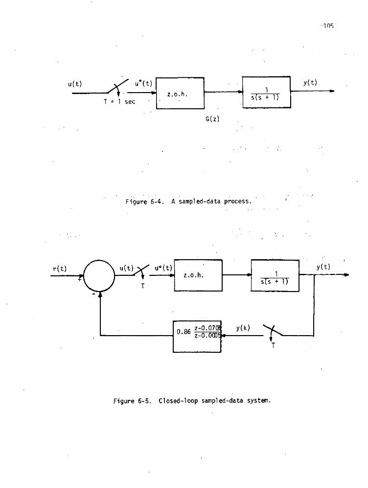
G ( z )

Figure 6-4. A sampled-data process.

•105

(t) V' u*(t)

" » *T = 1 sec

z.o.h.1

s(s + 1)

y(t)

r(t)z.o.h.

s(s

0.86 Z-0.07CBz-O.OOOE

y(k)

y( t )

Figure 6-5. Closed-loop sampled-data system.

106

. .7. A Numerical Technique for Predicting Self-Sustained Oscillations

/in the Nonlinear LSI System With the Continuous and .Discrete

Describing Function Methods \ . ., '' V" • '\

7.1 Introduction \ ,.

It has been demonstrated [2] that the continuous and discretei " •

describing function methods are useful tools for predicting the

existence of self-sustained oscillations due to the nonlinear CMG! \

friction in a single-axis model of the LSI. The corresponding stability

equations which have to be solved are _______^

1 + N(A)G(jw) = 0 (continuous case) - - (7-1)

and •' i

1 + N(A, n)G(T, ,n) = 0 (discrete case) . . (7-2). /'•

In Reference [2], these equations' were solved graphically, and the

conditions for existence of selfrsustained oscillations were established./

In each case the intersection of the -1/N curves with the G curves of

the system was used as a criterjion for the solution of the stability^-

equations, (7-1) and (7-2).i "

Although this approach is'convenient in the case of a single

nonlinearity, it becomes very/cumbersome, if not impossible to use,

when more than one nonlinearity exists, except in a few special

cases [8]. For example, witfi two coupled 1ST axes, the stability

equations in the continuous1 case may be of the form,

1 + G1(jo))N(A) + G2(j(i)N2(A) = 0 (7-3)

I

Clearly, a graphical solution for Eq. (7-3) is impractical, and .

107

the situation very quickly deteriorates if more axes are added, or

if the amplitudes of oscillations in the different axes are not the

same.

In view of this situation, it appears worthwhile to consider an

alternate method for solving the stability equations of the type of

(7-1) through (7-3). In this chapter the results obtained by solving

Eqs. (7-1) and (7-2) for the single-axis 1ST system by means of an

iterative numerical method are presented. This method has been

successful and provides numerical solutions to Eqs. (7-1) and (7-2),

these solutions being identical to those obtained by the earlier

graphical method. The method is promising and can be directly extended

to the more complicated cases, as in Eq. (7-3).

7-2 The Numerical Method

Consider the set of two nonlinear equations

f (it y \ = n1 i V AT , A«-> / u

x2) = 0

or in more compact notation

F(x).= 0

where

(7-4)

(7-5)

F ='1

V

, x = (7-6^

An algorithm for an iterative solution of Eqs. (7-4) or (7-5) is

(7-7)

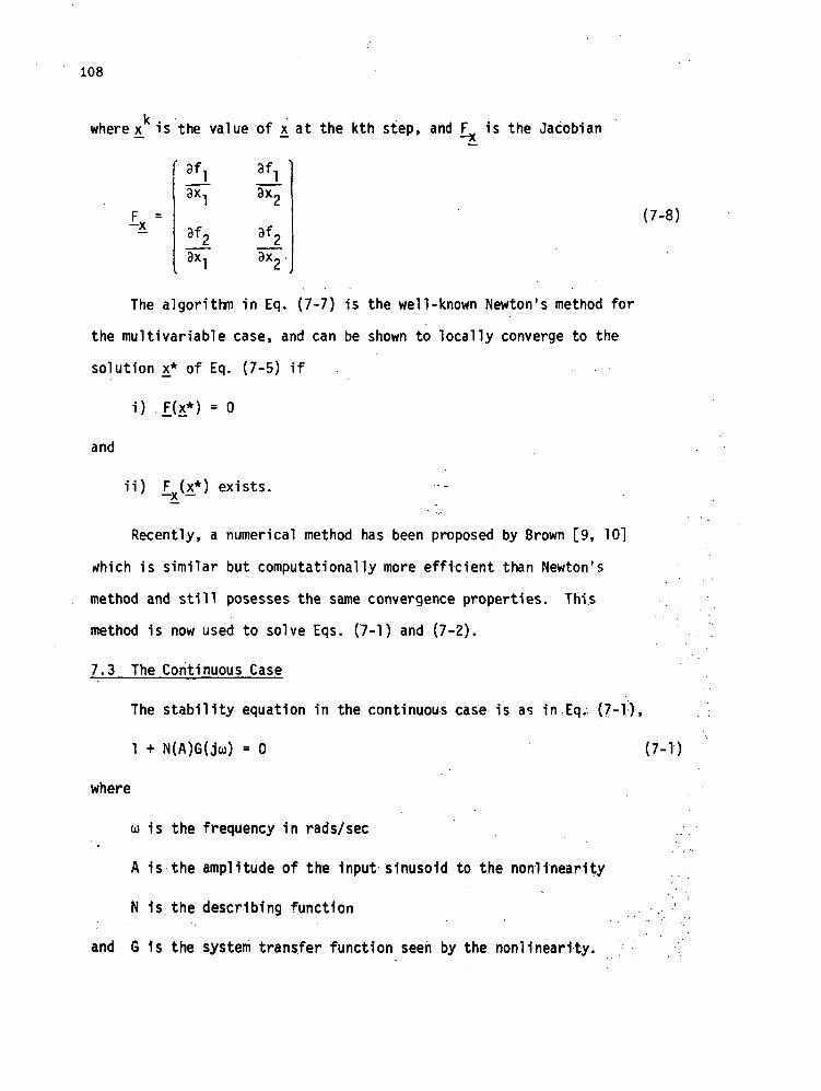
108

where x^ is the value of x. at the kth step, and £ is the Jacobian

3f, 9f,

fx-

l

(7-8)

The algorithm in Eq. (7-7) is the well-known Newton's method for

the multivariable case, and can be shown to locally converge to the

solution 21* of Eq. (7-5) if

i) £(x*) = 0

and

ii) £ (x*) exists. -}\ '

Recently, a numerical method has been proposed by Brown [9, 10]

rfhich is similar but computationally more efficient than Newton's

method and still posesses the same convergence properties. This

method is now used to solve Eqs. (7-1) and (7-2).

7.3 The Continuous Case

The stability equation in the continuous case is as in:Eq. (7-1)»

1 + N(A)G(juj) = 0 (7-1)

where

u is the frequency in rads/sec

A 1s the amplitude of the input sinusoid to the nonlinearlty

N 1s the describing function '

and 6 1s the system transfer function seen by the nonllhearity.

109

Since N and 6 are both complex quantities, they may be written as

N(A) = NR(A) + jNj(A)

6(ju>) = GR(ju>) + jGjtJu)

where NR, N,, GR, and Gj are all real quantities.,

Substituting Eq. (7-9) into Eq. (7-1) yields

1 +JNR + jNj)(GR + jGj) = 0

(7-9)

(7-10)

Collecting the real and imaginary terms in Eq. (7-10) and equating

them to zero gives

1 + NR(A)GR(jo>) - Nj

jO) + N I (A)GR ( jo ) ) = 0

Using the notation' of Eq. (7-5), Eq. (7-11) becomes

1 0 "

0. C. \ C.' j ^ ;•

where

F(x)

2 1 * ^ 2

f] = 1,.> NRGR - -

(7-11)

(7-12)

= A (7-13)

thus, Eq. :(7-ll) represents a system of two simultaneous nonlinear

equations in two unknowns. This system is solved by the proposed numerical

110

method with the foil owing system .parameters

TGFO = O.I ft-ib

H = 600 ft-lb-sec

< J = 2.1 ft-lb-sec2

KQ =5758.35

= 1371.02

K = 216 ft-lb/rad/sec

Kj = 8700 .ft-lb/rad

Jv = 105 ft-lb-sec2 \ \ V."^"--

With y = 1.38 x 10 , it is known from the graphical results [2]

that two solutions to Eq. (7-11) exist. Figures 7-1 and 7-2 show the

numerical iterations for several initial solutions. The two solutions

are

1. u = 4.27 rad/sec

A = 5.57 x 10"6 rad

2. u = 1.748 rad/sec

A = 4.45 x lo"7 rad

Although solution 2 is an unstable equilibrium and solution 1 is

a stable equilibrium, the numerical method does not differentiate between

them. It converges on the solution in whose domain of attraction the

inital solution is chosen. Figure 7-3 shows a graphical interpretation

of the domains of attraction of the two solutions. If the initial

LST SYSTEM-NUMERICflL SOLUTION OF l+M<fl>G<V>-0.GflMMfl- 1.380000 07

Hi

ITERflTJClN FREQUENCY flMPLITUDE0 0.4 000 00000 OD 01 0 .,1.0000000000-041 0.4153389340D 01 0.95 057347 180- 06

•£ 0. 357261 1372D 01 0.2092881357D-053 0.405244S838D 01 0 .38447861430-054 0.4215366015D 01 0 .50985800730-055 0.42681575500 01 0 .55380613010-056 0.4272124884D 01 0 .55732954420-057 0.4272145403D 01 0 .5573466150D-05

MD= 1 FREQUEMCY* 4.27215D OORflD/SEC flMPLITUDE-

LST SYSTEH-HUMERICflL SOLUTIOM OF l*M<fl>G<:W)=0.GflMMfl* 1 .38000D 07

ITFWRTIOM FREQUENCY flMPLITUDE0 0.5000000000D 01 0 . 1000000000D-041 0.3954 07776 ID 01 0.3288577583D-052 0.4170249852D 01 0 .47549141690-053 0.4260352606D 01 0.5468966540r-054 0.4271 95299 OD 01 0 .5571790199D-055 0.4272145453D 01 0 .5573467 104D- 056 0.4272145393D 01 0 .5573465998D-05

Ni)= 1 FREQUENCY* 4.27215D OORftD/SEC flMPLITUDE-

LST SYSTEM-MUMERICflL SOLUTIOM OF l+M<fl)G<y)=0.GflWW» 1 .38000D 07

ITERflTIDM FREQUENCY flMPLITUDE0 0.6000000000D 01 0 .1 OOOOOOOOOD-041 0. 44647 04973D 01 0 .70748545520-052 0.4233 07 1867D 01 0 .52308067680-053 0.4270025323D 01 0 .55547703020-054 0.42721 4 0286D 01 0.55734268280-055 0.4272145395D 01 0 .55734660330-05

MD= 1 FREQUENCY- 4.27215D OORflD/SEC flMPLITUDE-

LST SYSTEM-MUMERICflL SOLUTION OF l+N<fl)G<W)=0.GflMMfl- 1 .380000 07

ITERflTION ' FREQUENCY ftMPLITUDE0 0.7000000000D 01 0.10000000000-041 0.4978234956D 01 0.99485952130-052 0.395 07536 09D 01 0.32653775340-053 0.4167741217D 01 0 .47374680190-054 0.4259855835D 01 0. 54645636 03D- 05"5 0.4271936111D 01 0.5571641673D-056 0.42721454530 01 0.557346 7 1590- 057 0.4272145393D 01 0.55V3465998D-05

ND= 1 FREQUENCY- 4.27215D OORflD/SEC flMPLITUDE-

5.57347D-06

5.57347D-06

5.573470-06

5.573470-06

-Figure 7-1. Numerical iterations in the continuous case;

Y = 1.38 x io7.

112

LST SYSTEM-MUMERICRL SOLUTION OFGRMMfl= 1 .33GOOD 07

ITERflTIOh01•-*l_

34

FREQUENCY0.5000000000D 010.4330824789D 010.4272669199D0.4272145539D0.4£7£145393D

010101

RMPLITUDE0.5000000000D-050.57160709£3D-050.5575178057D-050.5573465283D-050.5573466GOOD-05

ND= 1 FREQUENCY= 4.27215D OORRD/SEC RMPLITUDE= 5.57347D-06

LST SYSTEM-NUMERICRL SOLUTION OF 1+N<:R>G<:W> =GRMMfl= 1.38000D 07

ITERRTION01£3456

FREQUENCY0.5000000000D0.3986281834D0.4081011589D0.42423334OOD0.4270849057D0.4272143796D0.4272145393D

RMPLITUDE01 0.1000000000D-0501 0.£781931045D-0501 0.4234094904D-0501 0.5306434465D-0501 0.5562073786D-0501 0.5573455629D-0501 0.5573466007D-05

ND= 1 FPEQUENCY= 4.27215D OORflD/SEC RMPLITUDE= 5.57347D-06

LST SYSTEM-NUMERICRL SOLUTION . D F 1 + N < R > G ( W ) =GRMMR= 1 .380OOD 07

ITERRTION012345

FREQUENCY0.3000000000D 010.4106761584D 010.4110062736D 010.4249871806D 010.4271417631D 010.4272145079D 010.4272145393D 01

RMPLITUDE0.1000000000D-050.3045086482D-050.4414687420D-050.5373028097D-050.5567084315D-050.5573465364D-050.5573465999D-05

MD= 1 FREQUENCY= 4.27215D OORRD^SEC RMPLITUDE= 5.57347D-06

LST SYSTEM-NUMERICRL SOLUTION OF l*N<fl)G<.W) =GRMMfl* 1.38GOOD 07

ITERRTION FREQUENCY0 0..2000000000D 01

0.1633524697D 010.1712930384D 010.17454660££D 010.1748094452D 010.1748104365D 01

ND= 1

1£345

RMPLITUDE0.5000000000D-060.2812970363D-060.4060843547D-060.4418355628D-060.4451098805D-060.4451182416D-06

FREQUENCY= 1.74810D OORRD/SEC RMPLITUDE= 4.45118D-0;

Figure 7-2. Numerical iterations in the continuous case;

Y = 1.38 x 107.

10

Ol

^ 6

OcOl3crO)t.

System 1 -.Y = 1.38 x 10

Solution 1

Solution 2 | •i ! ;

:

) ' :

I

i

t i 10 2 4 6 8 1 (

Amplitude (*10~ )

Figure 7-3. Domains of attraction of the two solutions with

Y = 1.38 x.io7.

12

114

conditions are chosen outside of the domain of attraction, the method

does not converge.

With changes in y, the solution points shift, and Fig. 7-4 shows

the stable solutions with y = 0.69 x 10° and 1.38 * 10 respectively.

7.4 The Discrete Case

In this case the input to the nonlinearity is assumed to be

e(t) = Acos(oit + 4) (7-14)

and the stability equation is

1 + N(A, <J>, n)G(T, n, z) = 0 (7-15)

where

T is the sampling period of the system

n is the order of oscillation, i.e., the period of oscillation is Tn.

A is the amplitude of the sinusoidal input to the nonlinearity

<t> is the phase of this input relation to the sampling process

z = exp(j2ir/nT)

G is the z-domain transfer function seen by the nonlinearity

N is the discrete describing function of the nonlinearityi

To maintain consistency, Eq. (7-15) can have two and only two

variables; thus, n and $ are assumed to be fixed parameters, and A and

T are the two variables. With each value of n and $, a solution of

Eq. (7-15) is desired.

As in the continuous case, define

G(T) = 6R(T) + jG j (T )

N(A) = NR(A) + jN j (A ) (7-16)

115LSI SYSTEM-MUMERICRL SOLUTION DF H-M<R>G<:W> =GRMMR= 6.90 GOOD 07

ITERRTIDM01£345

FREQUENCY0.7000000000D 010.5323793060D 010.520.3573337D 010.5220917925D 010.5221777385D 010.5221 77888 OD 01

RMPLITUDE0 . 1 OOOOOOOOOD-040.10644954970-040 .81 13476180D-050.35567416220-050 .8580953482D-050 .85809971 1 3D- 05'

HD= 1 FREQUENCY^ 5.221780 OORRD'SEC RMPLITUDE= 8.58100D-06

LST SYSTEM-HUMERICRL SDLUTIDM DF 1*M<R>G<.W)GRMMR= 6.90000D 07

ITERRTIDM FREQUENCY0 0.5000000000D 011 0. 520480881 OD 012 0.5221 £706190 013 0.5221778574D 014 0.5221778879D 01

flMPLITUDE0 .1 OOOOOOOOOD-040 .8217060863D-050 .8566684 03 ID- 050 .S580987575D-050 .85809970800-05

MD= 1 FREQUENCY^ 5.22178D OORRD/SEC RMPLITUDE= 8.58100D-06

LST SYSTEM-NUMERICRL SOLUTION DF l+M<.R>6rW>GRMMR= 1 .3800 OD 08

ITERRTIDN FREQUENCY0 0 . 7 0 0 0 0 0 0 0 0 0 D 011 0.54636941 240 0.12 CI.5412668486D 013 0. 54 1931 659 OD 014 0.5419498774D 015 0.541 94987 19D ,01

RMPLITUDE0 . 1 OOOOOOOOOD-040 . 1 07465 0663D- 040 .88942014140-050 .91559586220-050.91634971730-050 .91634959370-05

HD= 1 FREQUENCY= 5.419500 OORRD.-rSEC AMPLITUDE* 9.16350D-06

LST SYSTEM-NUMERICRL SOLUTION OF 1*N<:R>G =GRMMfl= 1 .330000 03

ITERRTION FREQUENCY0 0.5000000000D 01

0.5396836346D 011234

0.'5419441243D 010.54194987630 010.54194987190 01

AMPLITUDE0 . 1 O O O O O O O O O D r 040.89926538200-050 .91615031 19D-05, '0.91634974350-050.91634959360-05

ND= 1 FREQLIENCY= 5.419500 OORRD- SEC RMPLITUOE= 9. 1635 OH- Ob

Figure 7-4. Numerical iterations in the continuous case;

Y = 0.69 x 108 and 1.38 x io8.

116

Substituting Eq. (7-16) into Eq. (7-15) and separating the real and

imaginary parts yields

0

0F(x) =

21 ' *2

where

fl ' } + NRGR - NIGI

f2 ' NRGI + NIGR

(7-17)

x2 » A (7-18)

Equation (7-17) now represents two equations in two unknowns and

can be solved by the proposed numerical method. With the same system

parameters as in the continuous case, and Y = 1.38 x 10 , a solution

for n = 20, ({> = 0 is obtained. The initial solution in this case is

obtained from a knowledge of the continuous system solution. This

solution, n = 20 and <j> = 0, is now used as an initial guess to determine

the solution for n = 18, <J> = 0, which is then used as an initial solution

to obtain the solution for n = 16, 4> = 0, and so on. Figures 7-5, 7-6

and 7-7 show the iterations for n = 20 through n =r;4. , Due to the different

characteristics of the odd-n and even-n solutions, the decrement or

increment of n is made in multiples of 2. This way, the solution for

all n can be obtained.

Once a solution is available for a particular n at c|) = p, the

<|>-space can be spanned by slowly varying <J> and using the previous

117

LST SYSTEM-NUMERICRL SOLUTION OF DISCRETE DESCRIBING FUNCTIONGRMMfl= 1.38000D 07 N= 20 PHI= 0.0

ITERRTION SRMPLING PERIOD0 0.60000000000-011 0.66350225840-012 0.66848495970-013 P.66841848P9D-PI4 0.66841853860-01

RMPLITUDE0. 10000000000-040.71683512840-050-. 739159141 ID- 050.7402030884D-050.7402032739D-05

ND= 1 SflMPLING PERIOD* 6.68419D-02SEC flMPLITUDE* 7.40203D-06

LST SYSTEM-NUMERICRL SOLUTION OF DISCRETE DESCRIBING FUNCTION:GRMfW= 1.38000D 07 N= 18 PHI= 0.0

ITERRTION SRNPLIN6 PERIOD0 0.6684185385D-011 0.7258981714D-012 0.7332495463D-013 0.7333309288D-014 0.7333308321D-01

RMPLITUDE0.7402032738D-050.783180082OD-050.7741965I860-050.7740553676D-050.7740556323D-05

ND= 1 SRMPLING PERIOD* 7.33331D-02SEC RMPLITUDE* 7.74056D-06

LST SYSTEM-NUMERICflL SOLUTION OF DISCRETE DESCRIBING FUNCTIONGflMMfl" 1.38000D 07 N= 16 PHI= 0.0

RMPLITUDE0.7740556318D-050.8308808703D-050.8182471046D-050.8180174756D-05

ITERRTIDN SflMPLING PERIOD0 0.7333308323D-01

0.8035141927D-010.81368103230-010.8138185695D-010.81381842290-01

1234 0.8180178901D-05

ND= 1 SflMPLING PERI00= 8.13818D-02SEC flMPLITUDE« 8.18018D-06

LST SYSTEM-NUMERICflL SOLUTION OF DISCRETE DESCRIBING FUNCTIONGflMMR« 1.38QOOD 07 N= 14 PHI= 0.0

RMPLITUDE0.8180178895D-050.89611265890-050.8758961044D-050.8754660548D-050.8754667872D-05 -

ITERRTION SRMPLING PERIOD0 d;8138184231D-01

0.9022050932D-010.9175128977D-010.9177880263D-010.917787785OD-01

123-4.

ND= 1 SRMPUNG PERIOD* 9.177880^-02SEC RMPLITUDE- 8.754670-06

Figure 7-5. Numerical iterations in the discrete case;

Y = 1.38 x 10 , 4» = 0, variable n.

118

LSI SYSTEM-NUMERICRL SOLUTION OF DISCRETE DESCRIBING FUNCTIONGRMMR» 1 .38000D 07 N= 12 PHI= 0.0

flMPLITUDE0.875466786ID-050.'?891276673D-050.9522086634D-050.9512652996D-050.95126658720-05

ITERRTION SRMPLIhG PERIOD0 0.91778773530-011 0.1033226304D 00

,10588870090 00105956962OD 003

4

0.0,0.1059569299D 00

ND= 1 SRMPLING PERIOD- 1.05957D-01SEC RMPLITUDE= 9.51267D-0*

LST SYSTEM-NUMERICAL SOLUTION OF DISCRETE DESCRIBING FUNCTIONGRIH1fl= 1.38000D 07 N= 10 PHI= 0.0

flMPLITUDE0.95126658350-050.11317085750-040.10563506960-040.1053796573D-040.10337963180-04

ITERATION SRMPLIMG PERIOD0 0.10595693000 00

0.12160123110.00126490871 ID 001267133857D 00

1234

0.0,0.12671355280 00

ND= 1 SRMPLING PERIOD" 1 .26714D-01SEC RMPLITUDE= 1.05380D-05

LST SYSTEM-NUMERICRL SOLUTION OF DISCRETE DESCRIBING FUNCTIONGRMMfl= 1.38000D 07 N= 8 PHI= 0.0

ITERATION01234

SRMPLING PERIOD0.1267135526D 000.1484753967D 000.15933914740 000.1604043798D 000.1604109954D 00

RMPLITUDE0.10537963200-040.13781469330-040.12106371470-040.12001356820-040.12000770010-04

ND= 1 SRMPLING PERIOD' 1.60411D-01SEC RMPLITUDE= 1.200080-05

LST SYSTEM-NUMERICRL SOLUTION OF DISCRETE DESCRIBING FUNCTION6RMMR- 1.38000D 07 N= 6

ITERATION SRMPLING PERIOD0 0.16041098850 001 0.1897914063D 002 0.2182241830D 003 0.22727503010 004 0.22773712250 005 0.2277376514D 00

PHI= 0.0RMPLITUDE

0.1200077106D-040.18786504420-040.1497205004D-040.14102726820-040.14039709580-040.1408969070D-04

ND= 1 SRMPLING PERIOD- 2.277380-01SEC RMPLITUDE= 1.408970-05


Y = 1.38 x lo7, <j> = 0, variable n.

119

LST SYSTEM-NUMERICflL SOLUTIONGRMHfl* 1.38000D 07 M« 4

ITERflTIDH SflHPLIWG PERIOD01234567

0.2277376508D 00Q.2545144363D 00Q.3119051493D 000.4186370592D 000.5071624020D 00Q.5354877655I) 000.537146916ID 000.5371503035D ,00

DF DISCRETE DESCRIBIH6 FUMCTIOMPHI- 0.0

flHPLITUDE0; 1408969073D-040.2792562588D-040.258422275ID-040.148276520ID-040.1557192198D-040.1584931294D-^,04a.l587070!593D-f!q40.1587076Q13D-64

MD= 1 SRMPLIN6 PERIOD- 5.37150D-01SEC flflPLITUDE- 1 .58708D-05

Figure 7-7. Numerical iterations in the discrete case;Y = 1.38 x io7, <() = 0, variable n.

120

solution as the initial guess for the next solution. The range of <t>

is 2-n/n for n even and ir/n for n odd. Figures 7-8 through 7-11 show

the iterations for n = 3 and variable <j>. A plot of all solutions of

T and A for h = 3 and various <f>'s is shown in Fig. 7-12. Here the

plots for n = 4, 6, 8 and 10 are also shown. As n increases the range

of <J> decreases and the plots of T and A with 41 as a parameter shrink

to single points. Figure 7-13 shows the plot of T and A with <J> = 0

for n = 10 through n = 100.

The plots of Figs. 7-12 and 7-13 can be used to determine the

frequency (2ir/nT) and amplitude (A) of self-sustained oscillations when

the sampling period T is given. They provide very concise information

on the conditions under which self-sustained oscillations can occur in

the discrete-data system. The corresponding solutions by the graphical

method require overlapping the -1/N and G curves for each n and checking

for intersection or containment.

As n increases beyond 100, the discrete solution asymptotes

towards the continuous solution.

7.5 Conclusions and Extensions

The results of the previous sections have demonstrated the ease

and effectiveness of the proposed numerical method. It provides the

exact frequency and amplitude of oscillation in comparison to the

approximate values obtained by the graphical technique. In the discrete

case particularly, the numerical approach provides the information in

a more convenient form. The frequency and amplitude combinations which

can exist for each value of sampling period are available from a single

curve.

121

The major limitation of the numerical method is the convergence

characteristics of the solutions. Unless an adequate initial solution

is available, no useful information can be obtained. The initial

solution must be near to or within the domain of attraction of the

exact solution. Once a solution is obtained, it is simple to slowly

vary the parameters and obtain all the desired solutions.

The method is unrestricted to the form of the stability equation

or the number of nonlinearities present. If adequate initial solutions

can be selected, this approach can yield useful results with.the more

complicated multiple-axis models of the LST.

122

LST SYSTEM-NUMERICflL SOLUTION DF DISCRETE DESCRIBING FUNCTIONGflMMft= 1.38QOOD 07 h= 3 PHI= 6.00000D 01

ITERflTIDN01234

SflMPLING PERIOD0.1000000000D 010.1206736268D 01Q.I246507649D 010.1247557574D 010.1247557444D 01

AMPLITUDE0.2000000000D-040.2180807968D-040.220096657OD-040.2201127396D-040.2201127250D-04

ND= 1 SflMPLING PERIOD* 1.24756D OOSEC AMPLITUDE* 2.20113D-05

LST SYSTEM-NUMERICflL SOLUTION OF DISCRETE DESCRIBING FUNCTIONGftMMfl* 1.38000D 07 N== 3

ITERflTION SflMPLING PERIOD0 0.1247557444D 011 0.7576140716D 002 0.8593652656D 003 0.8710667172D 004 0.8711804237D 005 0.8711803498D 00

PHI= 5.00000D 01flMPLITUDE

0.2201127250D-040.2210012199D-040.2212015179D-040.2219934845D-040.2220037576D-040.2220037467D-04

ND= 1 SRMPLING PERIOD* 8.71180D-01SEC flMPLITUDE" 2.22004D-05

LST SYSTEM-NUMERICftL SOLUTION DF DISCRETE DESCRIBING FUNCTIONGflMHfl* 1.38000D 07 N= 3 PHI= 4.00000D 01

ITERflTIDN SflMPLING PERIOD AMPLITUDE00000000

0.6527844416L 00

0123.4

3711803498D6048096982D6S00626463D652778725OD

0,0,.2220037468D-04.229910346OD-04

0.2334330100D-040.234266340ID-040.2342710075D-04

ND= SflMPLING PERIOD- 6.527840-01SEC flMPLITUDE= 2.34271D-05

Figure 7-8. Numerical iterations in the discrete case;Y = 1.38 x 10 , n = 3, variable 4>.

123

LSI SYSTEM-NUMERICRL SOLUTION OF DISCRETE DESCRIBING FUNCTIONGRMMR- 1.38000D 07 N= 3 PHI= 3.00000D 01

ITERRTION SRMPLING PERIOD RMPLITUDE0000000000

01£34

0.6527844384D0.4972491700D0.5185445957D0.5191962437D0.5191954834D

0.2342710022D-040.2522386042D-040.2594052161D-040.2604023247D-040.2604065065D-Q4

ND* SRMPLING PERIOD- 5.19195D-01SEC RMPLITUDE* 2.60407D-05

LST SYSTEM-NUMERICRL SOLUTION OF DISCRETE DESCRIBING FUNCTIONGRMMR* 1.38000D 07 h= 3

ITERRTION SRMPLING PERIOD0 0.5191954849D 001 0.4479887235D 002 0.4542599663D 003 0.454254854ID 004 0.4542548401D 00

PHI= 2.00000D 01RMPLITUDE

0.2604065029D-040.2776194476D-04

, 0.2331780647D-040.2835057365D-040.2835057996D-04

ND= 1 SRMPLING PERIOD* 4.54255D-01SEC RMPLITUDE* 2.83506D-05

LST SYSTEM-NUMERICRL SOLUTIONGRMMR* 1.38000D 07 .N« 3

ITERRTION SRMPLING PERIOD0 0.4542548402D 001 0.6655150491D 002 0.7303889506D 003 0.6664793457D 004 0.6559819499D 005 0.655378Q327D 006 0.6553777502D 00

OF DISCRETE DESCRIBING FUNCTIONPHI= l . O O O O O D 01

RMPLITUDE0.2835057996D-040.1157357946D-040.1642213821D-040.1959748765D-040.2045437953D-Q40.2049946525D-040.2049953882D-04

ND= 1 SRMPLING PERIOD" 6 .55378D-01SEC RMPLITUDE* 2.04995D-05

Figune 7-9. Numerical iterations in the discrete case;

Y = 1.38 x 10 , n = 3, variable 4).

124

1.2

1.0

0.8

0.6

0.4

0.2

N = 10N = 8

N =

Amplitude (*10~5)

Figure 7-12. Amplitude and frequency (2ir/nT) of self sustained

oscillations for various sampling periods in the

discrete case; Y = 1 . 3 8 x l O , n = 3 through n = 10.

125

LSI SYSTEM-NUMERICflL SOLUTION OF DISCRETE DESCRIBING FUNCTIONGRMMR= 1.38GOOD 07 N= 3

ITERRTION SRMPLINb PERIOD0 0.9443921729D 001 0.1098499702D 012 0.11204229830 013 0.1120755444D 014 0.1120755263D 01

PHI= 4.00000D 00. RMPLITUDE

0.2000431869D-040.2069887736D-040.207522779ID-040.2075252072D-040.2075252039D-04

ND= 1 SflMPLING PERIOD= 1.12076D OOSEC RMPLITUDE= 2.075250-05

LST SYSTEM-NUMERICAL SOLUTION OF DISCRETE DESCRIBING FUNCTIONGRMMR= 1.38000D 07 N= 3

ITERRTION SRMPLING PERIOD0 0.1120755263D 011 0.1243920308D 012 0.1255495749D 013 0.1255574083D 01

PHI= 2 . 0 0 0 0 0 D 00RMPLITUDE

0.2075252039D-040.2159514112D-040.2162959060D-040.2162960044D-04

ND= 1 SRMPLING PERIOD" 1 .25557D OOSEC RMPLITUDE<= 2.16296D-05


Y = 1.38 x 10 , n = 3, variable <)»,

126

LST SYSTEM-NUMERICflL SOLUTION DF DISCRETE DESCRIBING FUNCTIONGRMMR= 1.38GOOD 07 N= 3

ITERRTIDN SRMPLING PERIOD0 0.600000GOOOD-001 0.6530111015D 002 0.65538590330 003 0.655377732OD 00

PHI= 1.000000 01ftMPLITUDE

0.£0000000000-040.20385448650-040.20498736630-040.£0499539530-04

ND= 1 SRMPLING PERIDD= 6.55378D-01SEC RNPLITUDE= 2.04995D-05

LST SYSTEM-NUMERICflL SOLUTION OF DISCRETE DESCRIBING FUNCTION6RMMR= 1.38000D 07 N= 3 PHI= 8.000000 00

x \flMPLITLIDE0.£0499538730-04

"0X.' 19589356720- 040.19821219190-040.19825498430-040.19825494370-04

ITERRTION SRMPLIhG PERIOD0 0. 65537775 18D 00

0.77035620410 00X

0.7841108478D 000.784207581 ID 000.7842075975D 00

1£34

ND= 1 JRMPLING PERIOD= 7.84208D-01SEC RrffL\ITUDE= 1.98£55D-05•\\ I

LST SYSTEM-NUMERICRL SOLUTION OF DISCRETE DESCRIBING FUNCTIONGRM«R= 1.38.0.0 OD 07 N= 3

ITERRTION01£34

SRMPLING PERIOD0.784£075974D 000.92358101280 000.94407l£6iID 000.9443923074D 000.9443921728D 00

PHI= 6.00000D 00RMPLITUDE

0.19825494380-040.19904826370-040.£0003132420-040.20004320190-040.20004318680-04

ND= 1 SRHPLING PERIQD= 9.443920-01SEC RNPLITUDE= £.000430-05

Figure 7-10. . Numerical iterations in the discrete case;

Y = 1.38 x 107, n = 3, variable <J>.

127

0.12 .-

Y = 1.38 x 10 , T« = 0.1

S 0.06

0.02 ...

Amplitude (xlo~6)

Figure 7-13. Amplitude and frequency (2ir/nT) of self sustained

oscillations for various sampling periods in the

discrete case; y = 1-38 x io7, n = 10 through n = 100.

128

References • •

1. HEAO Supplemental Information: Gimbal Control System Analysis, Sperry

Flight Systems Division, Pheonix, Arizona, May, 1972.

2. B. C. Kuo and G. Singh, Continuous and Discrete Describing Function

Analysis of the LSI System, Final Report, for NAS8-29853, Systems

Research Laboratory, Champaign, Illinois, January 1, 1974.

3. B. D. 0. Anderson and J. B. Moore, Linear Optimal Control, Prentice-

Hall, Inc., Englewood Cliffs, N.J., 1971.

4. M. Healey, 'Study of Methods of Computing Transition Matrices',

Proceedings IEE, Vol. 120, No, 8, August, 1973, pp. 905-912.\

5. B. C. Kuo, G. Singh, R. A. Yackel, Research Study^ Stabilization

and Control-Modern Sampled-Data Control Theory,Tinal Report for

NAS8-28584, Systems Research Laboratory,-Champaign, Illinois,

April, 1973.

6. B. C. Kuo, G. Singh, and R. A. Yackel, "Digital Approximation of

Continuous-Data Systems by Point-by-Point State Comparison,"

Computer and Electrical Engineering, Vol. 1, pp. 155-170, 1973.

7. B . C . Kuo and G. Singh, Design of the Large Space Telescope Control

System, Bimonthly Report 1-74, for NAS8-29853, Systems Research

Laboratory, Champaign, Illinois, March 1, 1974.

8. E. J. Davison and D. Constantinescu, "A Describing Function Technique

for Multiple Nonlinearities in a Single-Loop Feedback System," IEEE

Transactions on Automatic Control, Vol. AC-16, February 1971, pp. 56-60.

129

9. K. M. Brown and S. D. Conte, "The Solution of Simultaneous Nonlinear

Equations," Proceedings ACM 22nd National Conference, pp. 111-114.

10. K. M. Brown, "Solution of Simultaneous Nonlinear Equations,"

Collected Algorithms from CACM. Algorithm 316.

•» V.S. UHJVKHNMKNT PRINTING OFFICE: 1974—635-044/32

NATIONAL. AERONAUTICS AND SPACE ADMINISTRATION

WASHINGTON. D.C. 2O546

OFFICIAL BUSINESS

PCNALTY FOR PRIVATE USE S300 SPECIAL FOURTH-CLASS RATE

BOOK

POSTAGE AND FEE* PAIDNATIONAL AERONAUTIC* AND

•PACE ADMINISTRATION4SI

POSTMASTER : If Undellverable (Section 158Postal Manual) Do Not Return

"The aeronautical and space activities of the United States shall beconducted so as to contribute . . . to the expansion of human knowl-edge of phenomena in the atmosphere and space. The Administrationshall provide for the widest practicable and appropriate disseminationof information concerning its activities and the results thereof."

—NATIONAL AERONAUTICS AND SPACE ACT OF 1958

NASA SCIENTIFIC AND TECHNICAL PUBLICATIONSTECHNICAL REPORTS: Scientific andtechnical information considered important,complete, and a lasting contribution to existingknowledge.

TECHNICAL NOTES: Information less broadin scope but nevertheless of importance as acontribution to existing knowledge.

TECHNICAL MEMORANDUMS:Information receiving limited distributionbecause of preliminary data, security classifica-tion, or other reasons. Also includes conferenceproceedings with either limited or unlimiteddistribution.

CONTRACTOR REPORTS: Scientific andtechnical information generated under a NASAcontract or grant and considered an importantcontribution to existing knowledge.

TECHNICAL TRANSLATIONS: Informationpublished in a foreign. language consideredto merit NASA distribution in English.

SPECIAL PUBLICATIONS: Informationderived from or of value to NASA activities.Publications include final reports of majorprojects, monographs, data compilations,handbooks, sourcebooks, and specialbibliographies.

TECHNOLOGY .UTILIZATIONPUBLICATIONS: Information on technologyused by NASA that may be of particularinterest in commercial and other non-aerospaceapplications. Publications include Tech Briefs,"Technology Utilization Reports andTechnology Surveys.

Details on the availability of these publications may be obtained from:

SCIENTIFIC AND TECHNICAL INFORMATION OFFICE

NATIONAL A E R O N A U T I C S AND S P A C E ADMIN ISTRATION

Washington, D.C. 20546

MODERN SAMPLED-DATA CONTROL THEORY: Design of the … · 2013-08-31 · NASA CONTRACTOR REPORT NASA...

Documents

Transcript of MODERN SAMPLED-DATA CONTROL THEORY: Design of the … · 2013-08-31 · NASA CONTRACTOR REPORT NASA...