Modern Robotics - Science Publishing Group
232
Transcript of Modern Robotics - Science Publishing Group


Modern Robotics
with OpenCV
Widodo Budiharto

Science Publishing Group
548 Fashion Avenue
New York, NY 10018
http://www.sciencepublishinggroup.com
Published by Science Publishing Group 2014
Copyright © Widodo Budiharto 2014
All rights reserved.
First Edition
ISBN: 978-1-940366-12-8
This work is licensed under the Creative Commons
Attribution-NonCommercial 3.0 Unported License. To view a copy of this
license, visit
http://creativecommons.org/licenses/by-nc/3.0/
or send a letter to:
Creative Commons
171 Second Street, Suite 300
San Francisco, California 94105
USA
To order additional copies of this book, please contact:
Science Publishing Group
http://www.sciencepublishinggroup.com
Printed and bound in India

http://www.sciencepublishinggroup.com III
Preface
Robotics is an interesting topic today. This book is written to provide an
introduction to intelligent robotics using OpenCV. This very useful book
intended for a first course in robot vision and covers modeling and
implementation of intelligent robot. The need for this textbook arose from
teaching robotics to student and hobbyist for many years and facing the
difficulty to provide excellent book to explain advanced technology in
intelligent robotics and kinematics of the robot.
This book differs from other robot vision textbooks:
Its content is consisting of many implementations of mobile robot and
manipulator using OpenCV.
Using newest technology in Microcontroller such as Propeller
Microcontroller for robotics.
Its content is consisting of introduction and implementation of OpenCV
described clearly.
This textbook is the result of many years of work, research, software
development, teaching and learning. Many people have influenced its outcome
in various ways. First, I must acknowledge my rector at Binus University, Prof.
Dr. Harjanto Prabowo for his support, and my supervisors and friends. Some of
my undergraduate students have also offered assistance to this book. Finally, a
word of recognition goes to parent, my wife, and my children Tasya, Shafira,
Aziz and Yusuf.
Jakarta-Indonesia, 2014
Dr. Widodo Budiharto1
1 Dr. Widodo Budiharto, School of Computer Science, Bina Nusantara University, Jakarta-Indonesia
Email: [email protected]


http://www.sciencepublishinggroup.com V
Contents
Preface ............................................................................................................... III
Chapter 1 Introduction to Intelligent Robotics.............................................. 1
Introduction ......................................................................................................... 3
History of Robot .................................................................................................. 3
Types of Robot .................................................................................................... 7
Embedded Systems for Robot ........................................................................... 12
Robot Vision ...................................................................................................... 15
Exercises ............................................................................................................ 18
References ......................................................................................................... 18
Chapter 2 Propeller Microcontroller ............................................................ 19
Introduction ....................................................................................................... 21
Introduction of Propeller Chip ........................................................................... 21
Programming the Propeller ................................................................................ 26
Exercises ............................................................................................................ 30
Reference ........................................................................................................... 31
Chapter 3 Basic Programming Robot .......................................................... 33
Introduction ....................................................................................................... 35
Robot’s Actuators .............................................................................................. 35
DC Motor........................................................................................................... 35
Servo Motor ....................................................................................................... 37
Programming Motors of Robot.......................................................................... 39
Sensors for Intelligent Robot ............................................................................. 43
Ultrasonic Distance Sensor: PING)))™ ......................................................... 43
Compass Module: 3-Axis HMC5883L .......................................................... 50
Gyroscope Module 3-Axis L3G4200D .......................................................... 54
PID Controller for the Robot ............................................................................. 61
Contents
VI http://www.sciencepublishinggroup.com
Exercises ............................................................................................................ 62
References ......................................................................................................... 62
Chapter 4 Serial Communication with Robot.............................................. 63
Introduction ....................................................................................................... 65
Serial Interface Using Microsoft Visual Basic/C# .Net ..................................... 65
Wireless Communication for Robot .................................................................. 72
433 MHz Transceiver .................................................................................... 72
XBee Transceiver ........................................................................................... 73
RN-42 Bluetooth Module .............................................................................. 74
Exercises ............................................................................................................ 75
References ......................................................................................................... 75
Chapter 5 Mechanics of Robots .................................................................... 77
Introduction ....................................................................................................... 79
Introduction of Gears ......................................................................................... 79
Types of Gears ................................................................................................... 81
Rack and Pinion Gears ................................................................................... 82
Arm Geometries ................................................................................................ 83
Kinematics of Robot .......................................................................................... 85
References ......................................................................................................... 85
Chapter 6 Introduction to OpenCV .............................................................. 87
Introduction ....................................................................................................... 89
Introduction of OpenCV .................................................................................... 90
Digital Image Processing ................................................................................... 97
Edge Detection ................................................................................................ 100
Optical Flow .................................................................................................... 105
References ....................................................................................................... 108
Chapter 7 Programming OpenCV .............................................................. 109
Introduction ..................................................................................................... 111
Morphological Filtering ................................................................................... 111

Contents
http://www.sciencepublishinggroup.com VII
Camshift for Tracking Object .......................................................................... 115
References ....................................................................................................... 122
Chapter 8 Extracting the Component’s Contours for Calculating Number
of Objects ........................................................................................................ 123
Introduction ..................................................................................................... 125
Introduction of Contours ................................................................................. 125
Counting Objects ............................................................................................. 127
References ....................................................................................................... 130
Chapter 9 Face Recognition Systems .......................................................... 131
Introduction ..................................................................................................... 133
Face Recognition in OpenCV .......................................................................... 133
Haar Cascade Classifier ................................................................................... 135
Face Features Detector .................................................................................... 144
Face Recognition Systems ............................................................................... 151
Rapid Object Detection with a Cascade of Boosted Classifiers Based on
Haar-like Features ........................................................................................... 152
Negative Samples ......................................................................................... 153
Positive Samples .......................................................................................... 153
Training ........................................................................................................ 156
Test Samples ................................................................................................ 158
Exercises .......................................................................................................... 159
References ....................................................................................................... 160
Chapter 10 Intelligent Humanoid Robot .................................................... 163
Introduction ..................................................................................................... 165
Humanoid Robot ............................................................................................. 165
The Architecture of the Humanoid Robot ....................................................... 167
Ball Distance Estimation and Tracking Algorithm ......................................... 170
A Framework of Multiple Moving Obstacles Avoidance Strategy ................. 171
Experiments ................................................................................................. 173
Object Detection Using Keypoint and Feature Matching ................................ 177

Contents
VIII http://www.sciencepublishinggroup.com
References ....................................................................................................... 183
Chapter 11 Vision-Based Obstacles Avoidance ......................................... 185
Introduction ..................................................................................................... 187
Obstacle Avoidance of Service Robot ............................................................. 187
Stereo Imaging Model ..................................................................................... 190
Probabilistic Robotics for Multiple Obstacle Avoidance Method ................... 192
Multiple Moving Obstacles Avoidance Method and Algorithm ..................... 193
Multiple Moving Obstacle Avoidance Using Stereo Vision ........................... 198
References ....................................................................................................... 201
Chapter 12 Vision-Based Manipulator ....................................................... 203
Introduction ..................................................................................................... 205
Inverse Kinematics .......................................................................................... 205
Vision-Based Manipulator ............................................................................... 206
Grasping Model ............................................................................................... 208
Exercise ........................................................................................................... 212
References ....................................................................................................... 213
Glossary .......................................................................................................... 215

Chapter 1
Introduction to Intelligent Robotics


http://www.sciencepublishinggroup.com 3
On successful completion of this course, students will be able to:
Explain history and definition of robot.
Describe types of robot.
Explain the newest technology of intelligent robotics.
Explain the concept of embedded system for robotics.
Introduction
Robotics technology increase drastically following the demand of intelligent
robotics that able to help human kind. For robots to be intelligent in the way
people are intelligent, they will have to learn about their world, and their own
ability to interact with it, much like people do. Robot vision is a branch of
robotics that learns about acquisition and image processing for intelligent
robotics. At 2030, it is predicted that almost home duty task accomplished by
service robot that use vision sensors such as camera, it is a big challenge for us
to develop that robot. A robot is a mechanical or virtual agent, usually an
electro-mechanical machine that is guided by a computer program or electronic
circuitry. Intelligent robotics is a system that contains sensors, camera, control
systems, manipulators, power supplies and software all working together to
perform a task. That’s why the ability to develop intelligent robotics using
computer vision is a must to for the future.
History of Robot
The term Artificial Intelligence or AI stirs emotions. In 1955, John McCarthy,
one of the pioneers of AI, was the first to define the term Artificial intelligence,
roughly as follows:
The goal of AI is to develop machines that behave as though
they were intelligent.
According to McCarthy’s definition the aforementioned robots can be
described as intelligent. The word of robot is very familiar with us today [1].
The term robot was first used to denote fictional automata in a 1921 play R.U.R.
Rossum's Universal Robots by the Czech writer, Karel Čapek. According to
Čapek, the word was created by his brother, Josef from the Czech "robota",

Modern Robotics with OpenCV
4 http://www.sciencepublishinggroup.com
meaning servitude. In 1927, Fritz Lang's Metropolis was released; the
Maschinenmensch ("machine-human"), a gynoid humanoid robot, also called
"Parody", "Robotrix", or the "Maria impersonator" (played by German actress
Brigitte Helm), was the first robot ever to be depicted on film [2].
Figure 1.1 R.U.R by Czech Writer [2].
The history of robots has its origins in the ancient world. The modern concept
began to be developed with the onset of the industrial revolution which allowed
for the use of complex mechanics and the subsequent introduction of electricity.
This made it possible to power machines with small compact motors. In the
early 20th century, the modern formulation of a humanoid robot was developed.
Today, it is now possible to envisage human sized robots with the capacity for
near human thoughts and movement.
At ~270BC an ancient Greek engineer named Ctesibus made organs and
water clocks with movable figures. Al-Jazari (1136–1206), a Muslim inventor
during the Artuqid dynasty, designed and constructed a number of automatic
machines, including kitchen appliances, musical automata powered by water,
and the first programmable humanoid robot in 1206. Al-Jazari's robot was a
boat with four automatic musicians that floated on a lake to entertain guests at
royal drinking parties. His mechanism had a programmable drum machine with
pegs (cams) that bump into little levers that operate the percussion. The
drummer could be made to play different rhythms and different drum patterns
by moving the pegs to different locations.

Chapter 1 Introduction to Intelligent Robotics
http://www.sciencepublishinggroup.com 5
Figure 1.2 Al-Jazari's toy boat, musical automata. The first humanoid robot claimed in
the world.
In Japan, complex animal and human automata were built between the 17th
to 19th centuries, with many described in the 18th century Karakuri zui. One
such automaton was the karakuri ningyō, a mechanized puppet.
Modern Robot glory starts from 1970, when Professor Victor Scheinman at
Stanford University designed the standard manipulator. Currently, the standard
kinematics configuration known as robotic arms is still used. Finally, in 2000
Honda showed off a robot that was built many years named ASIMO, and is
followed by Sony AIBO robot dog.

Modern Robotics with OpenCV
6 http://www.sciencepublishinggroup.com
Figure 1.3 Karakuri, robot from Japan.

Chapter 1 Introduction to Intelligent Robotics
http://www.sciencepublishinggroup.com 7
Table 1.1 The timeline of robotics development.
No. Year Description
1 1495 Around 1495 Leonardo da Vinci sketched plans for a humanoid robot.
2 1920
Karel Capek coins the word ‘robot’ to describe machines that resemble
humans in his play called Rossums Universal Robots. The play was about
a society that became enslaved by the robots that once served them.
3 1937 Alan Turing releases his paper “On Computable Numbers” which begins
the computer revolution.
4 1997 On May 11, a computer built by IBM known as Deep Blue beat world
chess champion Garry Kasparov.
5 1999
Sony releases the first version of AIBO, a robotic dog with the ability to
learn, entertain and communicate with its owner. More advanced versions
have followed.
6 2000 Honda debuts ASIMO, the next generation in its series of humanoid
robots.
7 2008
After being first introduced in 2002, the popular Roomba robotic vacuum
cleaner has sold over 2.5 million units, proving that there is a strong
demand for this type of domestic robotic technology.
8 2011
The first service robot from Indonesia named Srikandi III with the stereo
vision system and multiple obstacles avoidance ability developet at ITS
Surabay.
9 2013 Intelligent telepresence robot developed at BINUS University from
collaboration of NUNI.
10 2014 Vision based grasping model for Manipulator developed at BINUS
University - Jakarta.
Types of Robot
Robot designed to fulfill user needs. Robot types can be divided into:
Manipulator robot, for example an arm robot.
Wheeled robot.
Walking robot.
Humanoid robot.
Aerial robot.

Modern Robotics with OpenCV
8 http://www.sciencepublishinggroup.com
Submarine robot.
A robot has these essential characteristics:
1) Sensing, First of all your robot would have to be able to sense its
surroundings. It would do this in ways that are not unsimilar to the way
that you sense your surroundings. Giving your robot sensors: light sensors
(eyes), touch and pressure sensors (hands), chemical sensors (nose),
hearing and sonar sensors (ears), and taste sensors (tongue) will give your
robot awareness of its environment.
2) Movement, A robot needs to be able to move around its environment.
Whether rolling on wheels, walking on legs or propelling by thrusters a
robot needs to be able to move. To count as a robot either the whole robot
moves, like the Sojourner or just parts of the robot moves, like the Canada
Arm.
3) Energy, A robot needs to be able to power itself. A robot might be solar
powered, electrically powered, battery powered. The way your robot gets
its energy will depend on what your robot needs to do.
4) Programmability, it can be programmed to accomplish a large variety of
tasks. After being programmed, it operates automatically.
5) Mechanical capability, Enabling it to act on its environment rather than
merely function as a data processing or computational device (a robot is
a machine).
6) Intelligence, A robot needs to be smart. This is where programming enters
the pictures. A programmer is the person who gives the robot its 'smarts.'
The robot will have to have some way to receive the program so that it
knows what it is to do.
A manipulator is a device used to manipulate materials without direct contact.
The applications were originally for dealing with radioactive or biohazardous
materials, using robotic arms, or they were used in inaccessible places. In more
recent developments they have been used in applications such as robotically-
assisted surgery and in space. It is an arm-like mechanism that consists of a
series of segments, usually sliding or jointed, which grasp and move objects
with a number of degrees of freedom.
Robot manipulators are created from a sequence of link and joint
combinations. The links are the rigid members connecting the joints, or axes.
The axes are the movable components of the robotic manipulator that cause
relative motion between adjoining links. The mechanical joints used to

Chapter 1 Introduction to Intelligent Robotics
http://www.sciencepublishinggroup.com 9
construct the robotic arm manipulator consist of five principal types. Two of the
joints are linear, in which the relative motion between adjacent links is non-
rotational, and three are rotary types, in which the relative motion involves
rotation between links.
The arm-and-body section of robotic manipulators is based on one of four
configurations. Each of these anatomies provides a different work envelope and
is suited for different applications.
1) Gantry - These robots have linear joints and are mounted overhead. They
are also called Cartesian and rectilinear robots.
2) Cylindrical - Named for the shape of its work envelope, cylindrical
anatomy robots are fashioned from linear joints that connect to a rotary
base joint.
3) Polar - The base joint of a polar robot allows for twisting and the joints are
a combination of rotary and linear types. The work space created by this
configuration is spherical.
4) Jointed-Arm - This is the most popular industrial robotic configuration.
The arm connects with a twisting joint, and the links within it are
connected with rotary joints. It is also called an articulated robot [3].
Figure 1.4 4 DOF Manipulator / arm robot from Lynxmotion suitable for education
(source: lynxmotion.com).
As the development of robot technology, the capability of the robot to "see"
or vision based robot has been developed such as ASIMO, a humanoid robot
created by Honda. With a height of 130 centimeters and weighs 54 kilograms,

Modern Robotics with OpenCV
10 http://www.sciencepublishinggroup.com
the robot resembles the appearance of an astronaut with the ability fingers
capable to handling egg. ASIMO can walk on two legs with a gait that
resembles a human to a speed of 6 km / h. ASIMO was created at Honda's
Research and Development Center in Wako Fundamental Technical Research
Center in Japan. The model is now the eleventh version, since the
commencement of the ASIMO project in 1986. According to Honda, ASIMO is
an acronym for "Advanced Step in Innovative Mobility" (a big step in the
innovative movement). This robot has a height of 130cm with a total of 34 DOF
and use 51.8V LI-ION rechargeable and the ability and mechanical grip better.
Figure 1.5 ASIMO Robot [4].
The rapid development of robot technology has demanded the presence of
intelligent robots capable of complement and assisted the work of man. The
ability to develop robots capable of interacting today is very important, for
example, the development of educational robot NAO from France and Darwin
OP from Korea. In the latest development of robot vision are generally

Chapter 1 Introduction to Intelligent Robotics
http://www.sciencepublishinggroup.com 11
humanoid form, requires the Linux embedded module that can process images
from the camera quickly. For example, Smart Humanoid robot package Ver. 2.0
for general-purpose robot soccer or created by authors who have the
specification:
CM-530 (Main Controller-ARM Cortex (32bits) with AX-12A (Robot
Exclusive Actuator, Dynamixel).
AX-18A (Robot Exclusive Actuator, Dynamixel).
Gyro Sensor (2 Axis) dan Distance measurement system.
RC-100A (Remote Controller).
Rechargeable Battery (11V, Li-Po, 1000mA/PCM).
Balance Battery Charger.
Humanoid Aluminum frame full set.
Gripper frame set.
1.7GHz Quad core ARM Cortex-A9 MPCore.
2GB Memory with Linux UBuntu.
6 x High speed USB2.0 Host port.
10/100Mbps Ethernet with RJ-45 LAN Jack.
Figure 1.6 Smart Humanoid ver 2.0 using embedded system and webcam based on
LINUX Ubuntu.

Modern Robotics with OpenCV
12 http://www.sciencepublishinggroup.com
Embedded Systems for Robot
The robotics system requires adequate processor capabilities such as the
ability of the processor speed, memory and I / O facilities. The figure below is a
block diagram of an intelligent robotics that can be built by beginners.
Figure 1.7 Embedded system for intelligent robotics.
From the picture above, the point is you can use a variety of microprocessor /
microcontroller to make the robot as smart as possible. You may use the
standard minimum systems such as Propeller, AVR, Basic Stamp, and Arm
Cortex with extraordinary abilities. All inputs are received by the sensors will
be processed by the microcontroller. Then through the programs that we have
made microprocessor / microcontroller will take action to the actuator such as a
robot arm and the robot legs or wheels. Wireless technology used for the
purposes of the above if the robot can transmit data or receive commands
remotely. While the PC / Laptop is used to program and perform computational
processes data / images with high speed, because it is not able to be done by a
standard microcontroller. To provide power supply to the robots, we can use dry
battery or solar cell. For the purposes of the experiment, can be used as a

Chapter 1 Introduction to Intelligent Robotics
http://www.sciencepublishinggroup.com 13
standard microcontroller for main robot controller as shown below using
Arduino Mega:
Figure 1.8 Single chip solution for robot using Arduino Mega.
The figure shows that the standard microcontroller technologies such as AVR,
Arduino or Propeller and Arm Cortex, can be used as the main controller of
mobile robots. Technology sensors and actuators can be handled well using a
microcontroller with I2C capability for data communication between the
microcontrollers with a serial devices others. Some considerations in choosing
the right microcontroller for the robot is the number of I / O, ADC capability,
and signal processing features, RAM and Flash program memory. In a complex
robot that requires a variety of sensors and large input the number, often takes
more than one controller, which uses the principle of master and slave. In this
model there is a 1 piece main controller which functions to coordinate the slave
microcontroller.
In general, to drive the robots there are several techniques such as:
Single wheel drive, which is only one front wheel that can move to the
right and to the left of the steering.

Modern Robotics with OpenCV
14 http://www.sciencepublishinggroup.com
Differential drive, where 2 wheels at the back to adjust the direction of
motion of the robot.
Synchronous drive, which can drive a 3 wheeled robot.
Pivot drive, It is composed of a four wheeled chassis and a platform that
can be raised or lowered.The wheels are driven by a motor for translation
motion in a straight line.
Tracked robot uses wheels tank.
Figure 1.10 Tank Robot DFRobot Rover ver.2 using Arduino and XBee for Wireless
Communication (source:robotshop.com).
Ackermaan steering, where the motion of the robot is controlled by the 2
front wheels and 2 rear wheels.
Omni directional drives, where the motion of the robot can be controlled 3
or 4 wheel system that can rotate in any direction, so that the orientation of
the robot remains. Omniwheel useful because the orientation of the robot is
fix with the standard wheel angle α1 = 0°,α2 = 120° and α3 = 240°. Global
frame [x, y] represents robot’s environment and the location of robot can
be represented as ( . The global velocity of robot can be represented
as .

Chapter 1 Introduction to Intelligent Robotics
http://www.sciencepublishinggroup.com 15
Figure 1.11 Mobile Robot with omni directional drive systems (source:
nexusrobot.com).
Robot Vision
There are several important terms in the robot vision interconnected,
including computer vision, machine vision and robot vision. Computer vision is
the most important technology in the future in the development of interactive
robots. Computer Vision is a field of knowledge that focuses on the field of
artificial intelligence and systems associated with acquisition and image
processing. Machine vision is implemented process technology for image -
based automatic inspection, process control, and guiding robots in various
industrial and domestic applications. Robot vision is the knowledge about the
application of computer vision in the robot. The robot needs vision information
to decide what action is to be performed. The application is currently in robot
vision are as robot navigation aids, search for the desired object, and other
environmental inspection. Vision on the robot becomes very important because
it received more detailed information than just the proximity sensor or other
sensors. For example, the robot is able to recognize whether the detected object
is a person's face or not. Furthermore, an advanced vision system on the robot
makes the robot can distinguish a face accurately (Face recognition system
using PCA method, LDA and others) [6] [10]. The processing of the input
image from the camera to have meaning for the robots known as visual
perception, starting from image acquisition, image preprocessing to obtain the

Modern Robotics with OpenCV
16 http://www.sciencepublishinggroup.com
desired image and noise-free, for example, feature extraction to interpretation as
shown in Figure 1.12. For example, for customer identification and avoidance
of multiple moving obstacles based vision, or to drive the servo actuator to steer
the camera as it leads to a face (face tracking) [4].
Figure 1.12 Perception model for a stereo vision [11].
An example of intelligent robotics is a humanoid robot HOAP-1 with stereo
vision for navigation system. HOAP-1 is a commercial humanoid robot from
Fujitsu Automation Ltd. and Fujitsu Laboratories Ltd. for behavior research. In
the vision sub-system of HOAP-1, the depth map generator calculate depth map
image from stereo images. The path planning sub-system generate a path from
the current position to the given goal position while avoid obstacles.
Figure 1.13 Example of Vision-based Navigation system for Humanoid robot
HOAP-1 [12].

Chapter 1 Introduction to Intelligent Robotics
http://www.sciencepublishinggroup.com 17
Another example is a telepresence robot developed by author as shown in
figure 1.14. The test was conducted by running Microsoft IIS and Google
Application Engine on the laptop. When the servers were ready, Master
Controller, implemented by using a laptop, opened the application through web
browser that support WebRTC and entered 192.168.1.101 which was the
address of both servers to open it. This is not a problem because the servers
were running on different ports. After the connections were established, Master
controller then received image and sound stream from the robot and sent back
image and sound from Master Controller web camera to the robot. Experiments
of intelligent telepresence robot had been tested by navigating the robot to staff
person and to avoid obstacles in the office. Face tracking and recognition based
on eigenspaces with 3 images every person had been used and a databases of the
images had been developed. The robot was controlled using integrated web
application (ASP.Net and WebRTC) from Master Control. With a high speed
Internet connection, simulated using wireless router that had speed around 1
Mbps, the result of video conferencing was noticeable smooth.
Figure 1.14 Intelligent Telepresence robot using omniwheel and controlled
using Web [11].
Images collected by a robot during the embodied object recognition scenario
often capture objects from a non- standard viewpoint, scale, or orientation. In
subsequent development, artificial intelligence for the robot to recognize and
understand the human voice, attentive to the various motion listener and able to
provide a natural response by the robot are challenge ahead to build future
robots.

Modern Robotics with OpenCV
18 http://www.sciencepublishinggroup.com
Exercises
1) Explain the history of robots.
2) Explain the roles of computer vision in robotics.
3) Describe types of drive systems for robot.
4) Develop a block diagram of tank robot using embedded system.
5) Find out the advantages of stereo vision.
References
[1] E. Wolfgang, Introduction to Artificial Intelligence, Springer Publisher, 2011.
[2] www.wikipedia.org.
[3] http://www.galileo.org/robotics/intro.html.
[4] Asimo.honda.com.
[5] Budiharto W., Santoso A., Purwanto D., Jazidie A., Multiple moving obstacles for
service robot using Stereo Vision, Telkomnika Journal, Vol. 9 no.3, 2011.
[6] M. Spong, Hutchinson & Vidyasagar, Robot Modelling and Control, Wiley, 2001.
[7] Daiki Ito, Robot Vision, Nova Publisher, 2009.
[8] Budiharto W., Santoso A., Purwanto D., Jazidie A., A Navigation System for
Service robot using Stereo Vision, International conference on Control,
Automation and Systems, Korea, pp 101-107, 2011.
[9] Hutchinson S., Hager G., Corke P., A tutorial on visual servo control, IEEE Trans.
On Robotics and Automation, vol. 12(5), pp. 651-670, 1996.
[10] Budiharto W., Purwanto D., Jazidie A., A Robust Obstacle Avoidance for Service
Robot using Bayesian Approach, International Journal of Advanced Robotic
Systems, Intech publisher, vol 8(1), 2011.
[11] Budiharto, W., The framework of Intelligent telepresence robot based on stereo
vision, Journal of Computer Science, vol. 8, pp. 2062-2067, 2012.
[12] Okada K., et.al, Walking Navigation System of Humanoid Robot using Stereo
Vision based Floor Recognition and Path Planning with Multi-Layered Body
Image, Proceedings of the 2003 IEEE International COnference on Intelligent
Robots and System, Nevada, 2003.

Chapter 2
Propeller Microcontroller


http://www.sciencepublishinggroup.com 21
On successful completion of this course, students will be able to:
Describe some of popular microcontrollers.
Explain how to program the Propeller Microcontroller.
Assembly a simple mobile robot using microcontroller.
Introduction
Microcontroller is the main controller for electronic devices today, including
robots. Microcontroller well-known and readily available today are AVR, PIC,
Arduino, Propeller, ATmega 8535, ATmega16, ATmega32 and Basic Stamp.
Some other well-known brands eg 16F877 PIC and Basic Stamp 2. Parallax
Propeller microcontroller from one of the latest generation 32-bit
microcontroller that is capable of computing high-speed data. This
microcontroller has many advantages especially can be used for image
processing. Therefore, this microcontroller is used as the main control system of
our robot.
Introduction of Propeller Chip
Do you like programming? With eight 32-bit processors in one chip,
integrating peripheral devices is suddenly simplified with the Propeller. A
Parallax creation from the silicon on up, the Propeller chip’s unique architecture
and languages will change the way you think about embedded system design.
The Propeller chip gives programmers both the power of true multi-processing
and deterministic control over the entire system.
Each of the Propeller chip’s processors, called cogs, can operate
simultaneously, both independently and cooperatively with other cogs, sharing
access to global memory and the system clock in a round-robin fashion through
a central hub. Each cog has access to all 32 I/O pins, with pin states being
tracked in its own input, output and direction registers. Each cog also has its
own memory, 2 counter modules, and a video generator module capable of
producing NTSC, PAL & VGA signals. Propeller Specifications:
Lanuages: Spin (native, object-based), Assembly (native low-level),
C/C++ (via PropGCC).

Modern Robotics with OpenCV
22 http://www.sciencepublishinggroup.com
Power Requirements: 3.3 VDC.
Operating Temperature: -55 to +125 degrees C.
Processors (Cogs): 8.
I/O Pins: 32 CMOS.
External Clock Speed: DC to 80 MHz.
Internal RC Oscillator: ~12 MHz or ~20 kHz.
Execution Speed: 0 to 160 MIPS (20 MIPS/cog).
Global ROM/RAM: 32768/32768 bytes.
Cog RAM: 512 x 32 bits/cog.
The Propeller is used in many industries including manufacturing, process
control, robotics, automotive and communications. Hobbyists and engineers
alike are finding new uses for this powerful microcontroller every day. The
Propeller is a good choice over other microcontrollers when a low system part
count is desirable due to its ability to provide direct video output and an easy
interface to external peripherals such as keyboard, mouse and VGA monitor.
Pre-written objects to support many types of hardware also make it an attractive
option. All of this plus low cost and a powerful, yet easy language are hard to
beat in a world where microcontrollers come in so many flavors that it’s hard to
make a choice.
The Propeller chip is a multicore microcontroller that is programmable in
high-level languages (Spin™ and C) as well as a low-level (Propeller assembly)
language. Application development is simplified by using the set of pre-built
objects for video (NTSC/PAL/VGA), mice, keyboards, LCDs, stepper motors
and sensors. Propeller is easily connected to your computer's serial or USB port
for programming using our Prop Plug. The Propeller chip can run on its own
with a 3.3-volt power supply, internal clock, and with its internal RAM for code
storage. Add an external EEPROM for non-volatile code storage and an external
clock source for accurate timing.
The Propeller Tool Software is the primary development environment for
Propeller programming in Spin and Assembly Language. It includes many
features to facilitate organized development of object-based applications: multi-
file editing, code and document comments, color-coded blocks, keyword
highlighting, and multiple window and monitor support aid in rapid code
development. We can use the board such as Propeller Robot board or Propeller

Chapter 2 Propeller Microcontroller
http://www.sciencepublishinggroup.com 23
Board of Education for learning Propeller easily for robotics as shown in figure
2.1.
(a)
(b)
Figure 2.1 Propeller Chip P8X32A in LQFP package (a) and Propeller Board of
Education (b).

Modern Robotics with OpenCV
24 http://www.sciencepublishinggroup.com
Table 2.1 pins description of propeller chip.
Pin Name Direction Description
PO-P31 I/O
General purpose I/O Port A. Can source/sink 40 mA
each at 3.3 VDC.
Logic threshold is ≈ VDD; 1.65 VDC @ 3.3 VDC.
The pins shown below have a special purpose upon
power-up/reset but are general purpose I/O afterwards.
P28 – 12C SCL connection to optional, external
EEPROM.
P29 – 12C SDA connection to optional, external
EEPROM.
P30 – Serial Tx to host.
P31 – Serial Rx from host.
VDD --- 3.3 volt power (2.7 – 3.3 VDC).
VSS --- Ground.
BOEn I
Brown Out Enable (active low). Must be connected to
either VDD or VSS. If low, RESn becomes a weak
output (delivering VDD through 5 KΩ) for monitoring
purposes but can still be driven low to cause reset. If
high, RESn is CMOS input with Schmitt Trigger.
RESn I/O
Reset (active low). When low, resets the Propeller chip:
all cogs disabled and I/O pins floating. Propeller restarts
50 ms after RESn transitions from low to high.
XI I
Crystal Input. Can be connected to output of
crystal/oscillator pack (with XO left disconnected), or
to one leg of crystal (with XO connected to other leg of
crystal or resonator) depending on CLK Register
settings. No external resistors or capacitors are required.
XO O
Crystal Output. Provides feedback for an external
crystal, or may be left disconnected depending on CLK
Register settings. No external resistors or capacitors are
required.
The Propeller 2 is a whole-system, high-speed mulitcore chip for future
embedded applications requiring real-time parallel control. Production
customers asked for features that are now standard in Propeller 2: A/D, code
protect, large RAM with freedom to download a C kernel or Spin interpreter
during program. With easy coding for video (VGA, composite and component
for HD), human interface devices, sensors and output devices, the Propeller 2 is

Chapter 2 Propeller Microcontroller
http://www.sciencepublishinggroup.com 25
effective for quick prototype and production projects with limited time to
market.
The Stingray robot from Parallax Inc. provides a mid-size platform for a wide
range of robotics projects and experiments. The Propeller Robot Control Board
is the brains of the system providing a multiprocessor control system capable of
performing multiple tasks at the same time. The Propeller chip provides eight
32-bit processors each with two counters, its own 2 KB local memory and 32
KB shared memory. This makes the Propeller a perfect choice for advanced
robotics and the Stingray robot. The board use is Propeller Robot Board
complete with the USB Programmer, 64KB EEPROM AT24C512 and DC
motor driver 7.2V as shown below:
Figure 2.2 Propeller Robot Control Board and the pins.
The general picture of the robot’s assembly to produce differential wheeled
robot models as shown below, and a complete description of the assembly can
be read from manual of this robot:

Modern Robotics with OpenCV
26 http://www.sciencepublishinggroup.com
Figure 2.3 The general description of asembleing the body, motors and the controller
of the robot.
Programming the Propeller
We need USB/Serial programmer to program this chip, note that the
connections to the external oscillator and EEPROM, which are enclosed in
dashed lines, are optional as shown in figure 2.4 or figure 2.5 for serial
programmer:

Chapter 2 Propeller Microcontroller
http://www.sciencepublishinggroup.com 27
Figure 2.4 The minimum system of Propeller DIP-40 and the programmer.
The cheapest programmer for Propeller show below:
Figure 2.5 Schematic of serial programmer for Propeller.

Modern Robotics with OpenCV
28 http://www.sciencepublishinggroup.com
After installing the Propeller tool software, the codes can be uploaded to the
chip by pressing F11 as shown below:
Figure 2.6 Programming the chip.
For basic experiments, we will try to program the LED lights on / off as well
as receive input from switches. Install LED lights and switches on the
protoboard are provided on the controller board as follows:
Figure 2.7 Schematic for basic testing of Propeller.
Here's an example of making light LED on / off at pin 4, save the file names
and contents LEDOnOffP4.spin by pressing F11, make sure the board Propeller
detected on the USB port of your computer:

Chapter 2 Propeller Microcontroller
http://www.sciencepublishinggroup.com 29
File: LEDOnOffP4.spin
PUB LedOnOff
dira[4] := 1 ' P4 → output
repeat
outa[4] := 1 ' P4 → on
waitcnt(clkfreq/4 + cnt) ' delay
outa[4] := 0 ' P4 → off
waitcnt(clkfreq/4 + cnt)
Figure 2.8 The USB connector and FTDI 232RL chip successfully detected the
microcontroller.
Use the LEDS, resistors and pluggable wires to create the circuit shown in
schematic below on the breadboard. The pluggable wires will jumper to the
breadboard to make the I/O and ground connections from the control board
locations shown below. Ground can be obtained from the bottom row of pins
(marked B) on the I/O headers. P0 and P1 are picked up from the top row
(marked W) and are indicated on the silkscreen on the control board. Power is
obtained from the center row (marked R) and its voltage is set by the jumper
immediately to the right of that group of headers.
Figure 2.9 The schematic for using standard transistor.

Modern Robotics with OpenCV
30 http://www.sciencepublishinggroup.com
The code for testing the transistor for driving LED shown below:
File: LED_Test.spin
CON
_xinfreq = 5_000_000 ' External Crystal freqwency
_clokmode = xtal1 + pll16x ' Enabled external crystal and PLL
x16
PUB Main
Dira[1..0] := %11 ' Set P0 and P1 to output
Repeat
Out[0] := 1 ' P0 HIGH
Outa[1] := 0 ' P1 LOW
Waitcnt (clkfreq/2 + cnt ) ' Delay ½ clock frequency (1/2
detik)
Out[0] :=0 ' P0 LOW
Outa[1] := 1 ' P1 HIGH
Waitcnt (clkfreq/2 + cnt ) ' Delay ½ clock frequency (1/2
detik)
The next example is made in P6 LED lights on / off dependent input from
P21, see what the output is generated when the switch is pressed in P21.
File: ButtonToLed.spin
PUB ButtonLED ' Pushbutton/LED Method
dira[6]:= 1 ' P6 → output
dira[21] := 0 ' P21 → input
repeat ' Endless loop
outa[6] := ina[21] ' Copy P21 input to P6 ouput
That is a basic example of programming using the Propeller chip, you have to
try other basic programming lies in the examples folder and library in the
Propeller Tool program.
Exercises
1) Describe and compare features of some popular microcontrollers.
2) Design a minimum system for mobile robot using Propeller chip.

Chapter 2 Propeller Microcontroller
http://www.sciencepublishinggroup.com 31
3) Create a program for Running LED using Propeller.
4) Create a program to control 2 DC Motors with an IC Driver L298 using
switch.
Reference
[1] Parallax.com.


Chapter 3
Basic Programming Robot


http://www.sciencepublishinggroup.com 35
On successful completion of this course, students will be able to:
Explain about robot’s actuators.
Program the sensors and motors for robot.
Introduction
Robot becomes a new trend of students and engineers, especially with a main
event and a robotics Olympiad each year. Programming the robot using
microcontroller is the basic principle of controlling the robot, where the
orientation of the microcontroller is to control the application of an information
system based on the inputs received, and processed by a microcontroller, and
the action performed on the output corresponding predetermined program.
Robot’s Actuators
Actuators are an important part of the robot that functions as an activator of
the command given by the controller. Usually, an electromechanical actuator
device produces movement. Actuator consists of two types:
Electric Actuators.
Pneumatic and Hydraulic Actuators.
In this sub-section will discuss the electric actuator which is often used as a
producer of such rotational motion of the motor.
DC Motor
A DC Motor in simple words is a device that converts direct current
(electrical energy) into mechanical energy. It’s of vital importance for the
industry today, and is equally important for engineers to look into the working
principle of DC motor in details. The very basic construction of a DC motor
contains a current carrying armature which is connected to the supply end
through commutator segments and brushes and placed within the north south
poles of a permanent or an electro-magnet as shown in the figure below:

Modern Robotics with OpenCV
36 http://www.sciencepublishinggroup.com
Figure 3.1 DC Motor diagram.
To understand the operating Principle of DC motor, it is important that we
have a clear understanding of Fleming’s left hand rule to determine the direction
of force acting on the armature conductors of dc motor. Fleming’s left hand rule
says that if we extend the index finger, middle finger and thumb of our left hand
in such a way that the current carrying conductor is placed in a magnetic field
(represented by the index finger) is perpendicular to the direction of current
(represented by the middle finger), then the conductor experiences a force in the
direction (represented by the thumb) mutually perpendicular to both the
direction of field and the current in the conductor.

Chapter 3 Basic Programming Robot
http://www.sciencepublishinggroup.com 37
Figure 3.2 Fleming’s left hand rule.
Figure below displays a DC motor with gearbox used on the robot to improve
torque:
Figure 3.3 An example of DC Motor with gearbox 7.2V 310RPM.
Servo Motor
Another important actuators are servo motors, which can work the wheel or
as a robot arm or gripper. Servo motors are often used is continuous Servo
Parallax, Parallax standard servo, GWS-S03, Hitec HS-805BB and HS-725BB.
Some of the grippers are often used in the lab. Robot gripper usually based on

Modern Robotics with OpenCV
38 http://www.sciencepublishinggroup.com
aluminum, lynxmotion robotic gripper hand and fingers are very popular as
follows:
(a) (b)
Figure 3.4 Lynxmotion robot hand RH1 with 2 servos (a) and gripper finger
using 5 servos to 14 joint (b).
Author recommends that you conduct experiments and make system-based
visual servoing robotic arm that can pick up an object using a robotic arm based
stereo camera. The robot arm is best used Dagu 6 degress of freedom and
AX18FCM5 Smart Robotic arm that uses the CM-5 controller, Full feedback
for position, speed, load, voltage and temperature, full control over position
(300 degrees), uses servo AX-18F and is compatible with MATLAB and other
common microcontroller systems.
(a) (b)
Figure 3.5 Dagu 6 degree freedom arm robotic system using aluminum Dagu gripper
(a) and AX18FCM5 Smart Robotic arm using CM-5 controller (b)[1].

Chapter 3 Basic Programming Robot
http://www.sciencepublishinggroup.com 39
Programming Motors of Robot
DC motors are usually driven by an H-Bridge since such a circuit can reverse
the polarity of the motor connected to it. The DC brushed motors included in
this kit are driven by the L6205 H-Bridge on the Propeller Robot Control Board.
Understanding how to control this H-Bridge is the key to controlling the
direction, speed and duration that the motors are on or off. Parallax has released
a Propeller object called, “PWM_32” which makes it easy to drive servos as
well as control motors using pulse width modulation. This object can be used
with the Propeller Robot Control Board to drive the on-board H-Bridge, which
in turn drives the DC motors.
The L6205 inputs are connected to P24 through P27 on the Propeller chip.
When the power switch on the control board is set for POWER ON/MOTORS
ON, the L6205 is enabled and the outputs are connected to the motors. The truth
table for controlling the L6205 is shown below in Table 3.1. P24 and P25
control the left motor while P26 and P27 control the right motor. This table
assumes the motors are connected to the control board as defined in the
assembly instructions.
Table 3.1 Motor truth table.
P24 P25 P26 P27 Left Motor Right Motor
0 0 0 0 Brake Brake
1 0 0 0 Reverse Brake
0 1 0 0 Forward Brake
1 1 0 0 Brake Brake
0 0 1 0 Brake Forward
1 0 1 0 Reverse Forward
0 1 1 0 Forward Forward
1 1 1 0 Brake Forward
0 0 0 1 Brake Reverse
1 0 0 1 Reverse Reverse
0 1 0 1 Forward Reverse
1 1 0 1 Brake Reverse
0 0 1 1 Brake Brake
1 0 1 1 Reverse Brake
0 1 1 1 Forward Brake
1 1 1 1 Brake Brake

Modern Robotics with OpenCV
40 http://www.sciencepublishinggroup.com
Note that it may be more intuitive to look at the table as two groups
consisting of P24/P25 and P26/P27. In this manner you have 4 possible
combinations for each motor as shown in Table 3.2.
Table 3.2 The value given to P24 and P25 and P26 and 27 for the motors.
P24 P25 Left Motor P26 P27 Right Motor
0 0 Brake 0 0 Brake
1 0 Reverse 1 0 Forward
0 1 Forward 0 1 Reverse
1 1 Brake 1 1 Brake
The program to make the left motor active is shown below:
File: LeftMotorTest.spin
CON
_xinfreq = 5_000_000
_clkmode =xtal1 + pll16x
PUB Main
Dira[27..24] := %1111 ' Set P24 – P27 to output
Outa [25] : = 1 ' Left motor forward
Waitcnt (clkfreq * 2 + cnt) ' 2 seconds pause
Outa [25] :=0 ' Left motor stop
Waitcnt (clkfreq * 2 + cnt)
Outa[24] :=1 ' Left motor reverse
Waitcnt (clkfreq * 2 + cnt)
Outa[24] :=0
repeat
To control the speed of a DC motor can use PWM (Pulse Width Modulation),
with the following example:
File : PWMx8.spin
CON
resolution = 256 'The number of steps in the pulse
widths. Must be an integer multiple of 4.
nlongs = resolution / 4

Chapter 3 Basic Programming Robot
http://www.sciencepublishinggroup.com 41
VAR
long fcb[5]
long pwmdata[nlongs]
long pinmask
long previndex[8]
byte cogno, basepin
PUB start(base, mask, freq)
' This method is used to setup the PWM driver and start its cog.
If a driver had
' already been started, it will be stopped first. The arguments
are as follows:
' base: The base pin of the PWM output block. Must be 0, 8,
16, or 24.
' mask: The enable mask for the eight pins in the block:
' bit 0 = basepin + 0
' bit 1 = basepin + 1
' ...
' bit 7 = basepin + 7
'
' Set a bit to 1 to enable the corresponding pin for
PWM ouput.
'
' freq: The frequency in Hz for the PWM output.
'
if (cogno)
stop
freq *= resolution
if (clkfreq =< 4000000 or freq > 20648881 or clkfreq < freq *
135 / 10 or clkfreq / freq > 40000 or base <> base & %11000 or
mask <> mask & $ff or resolution <> resolution & $7ffffffc)
return false
basepin := base
pinmask := mask << base
longfill(@pwmdata, 0, nlongs)
longfill(@previndex, 0, 8)
fcb[0] := nlongs
fcb[1] := freq
fcb[2] := constant(1 << 29 | 1 << 28) | base << 6 | mask

Modern Robotics with OpenCV
42 http://www.sciencepublishinggroup.com
fcb[3] := pinmask
fcb[4] := @pwmdata
if (cogno := cognew(@pwm, @fcb) + 1)
return true
else
return false
PUB stop
' This method is used to stop an already-started PWM driver. It
returns true if
' a driver was running; false, otherwise.
if (cogno)
cogstop(cogno - 1)
cogno~
return true
else
return false
PUB duty(pinno, value) | vindex, pindex, i, mask, unmask
' This method defines a pin's duty cycle. It's arguments are:
' pinno: The pin number of the PWM output to modify.
' value: The new duty cycle (0 = 0% to resolution = 100%)
' Returns true on success; false, if pinno or value is invalid.
if (1 << pinno & pinmask == 0 or value < 0 or value >
resolution)
return false
pinno -= basepin
mask := $01010101 << pinno
unmask := !mask
vindex := value >> 2
pindex := previndex[pinno]
if (vindex > pindex)
repeat i from pindex to vindex - 1
pwmdata[i] |= mask
elseif (vindex < pindex)
repeat i from pindex to vindex + 1
pwmdata[i] &= unmask

Chapter 3 Basic Programming Robot
http://www.sciencepublishinggroup.com 43
pwmdata[vindex] := pwmdata[vindex] & unmask | mask &
($ffffffff >> (31 - ((value & 3) << 3)) >> 1)
previndex[pinno] := vindex
return true
Sensors for Intelligent Robot
Ultrasonic Distance Sensor: PING)))™
PING)))™ ultrasonic sensor provides an easy method of distance
measurement. This sensor is perfect for any number of applications that require
you to perform measurements between moving or stationary objects. Interfacing
to a microcontroller is a snap. A single I/O pin is used to trigger an ultrasonic
burst (well above human hearing) and then "listen" for the echo return pulse.
The sensor measures the time required for the echo return, and returns this value
to the microcontroller as a variable-width pulse via the same I/O pin. The
PING))) sensor works by transmitting an ultrasonic (well above human hearing
range) burst and providing an output pulse that corresponds to the time required
for the burst echo to return to the sensor. By measuring the echo pulse width,
the distance to target can easily be calculated.
Key Features:
Provides precise, non-contact distance measurements within a 2 cm to 3 m
range for robotics application.
Ultrasonic measurements work in any lighting condition, making this a
good choice to supplement infrared object detectors.
Simple pulse in/pulse out communication requires just one I/O pin.
Burst indicator LED shows measurement in progress.
3-pin header makes it easy to connect to a development board, directly or
with an extension cable, no soldering required.
The PING))) sensor detects objects by emitting a short ultrasonic burst and
then "listening" for the echo. Under control of a host microcontroller (trigger
pulse), the sensor emits a short 40 kHz (ultrasonic) burst. This burst travels
through the air, hits an object and then bounces back to the sensor. The PING)))
sensor provides an output pulse to the host that will terminate when the echo is
detected, hence the width of this pulse corresponds to the distance to the target.

Modern Robotics with OpenCV
44 http://www.sciencepublishinggroup.com
Figure 3.6 The basic principle of ultrasonic distance sensor [2].
Figure 3.7 Communication protocol of the PING))).
This circuit allows you to quickly connect your PING))) sensor to a BASIC
Stamp/Propeller Board. The PING))) module’s GND pin connects to Vss, the 5
V pin connects to Vdd, and the SIG pin connects to I/O pin P15.

Chapter 3 Basic Programming Robot
http://www.sciencepublishinggroup.com 45
Figure 3.8 PING))) to the board.
Here is an example of using the Ping sensor shown in Serial LCD 4x20.
File: Ping_Demo.spin
CON
_clkmode = xtal1 + pll16x
_xinfreq = 5_000_000
PING_Pin = 15 ' I/O Pin For PING)))
LCD_Pin = 1 ' I/O Pin For LCD
LCD_Baud = 19_200 ' LCD Baud Rate
LCD_Lines = 4 ' Parallax 4X20 Serial LCD (#27979)
VAR
long range
OBJ
LCD: "debug_lcd"
ping: "ping"
PUB Start
LCD.init(LCD_Pin, LCD_Baud, LCD_Lines) ' Initialize LCD
Object
LCD.cursor(0) ' Turn Off Cursor
LCD.backlight(true) ' Turn On Backlight
LCD.cls ' Clear Display
LCD.str(string("PING))) Demo", 13, 13, "Inches -", 13,
"Centimeters -"))

Modern Robotics with OpenCV
46 http://www.sciencepublishinggroup.com
repeat ' Repeat Forever
LCD.gotoxy(15, 2) ' Position Cursor
range := ping.Inches(PING_Pin) ' Get Range In Inches
LCD.decx(range, 2) ' Print Inches
LCD.str(string(".0 ")) ' Pad For Clarity
LCD.gotoxy(14, 3) ' Position Cursor
range := ping.Millimeters(PING_Pin) ' Get Range In
Millimeters
LCD.decf(range / 10, 3) ' Print Whole Part
LCD.putc(".") ' Print Decimal Point
LCD.decx(range // 10, 1) ' Print Fractional Part
waitcnt(clkfreq / 10 + cnt) ' Pause 1/10 Second
Robot avoider is a robot that able to avoid the obstacle at the in front of the
robot or at the left or right side of the robot. Here's an example using a PING)))
as an avoider robot that only able to detect the obstacle in front of the robot
using 1 PING))).
Serial_LCD_Avoider.spin:
‘ Copyright Dr. Widodo Budiharto
‘ www.toko-elektronika.com 2014
CON
_clkmode = xtal1 + pll16x
_xinfreq = 5_000_000
LCD_PIN = 23
PING_Pin = 13 ' I/O Pin For PING)))
LCD_Baud = 19_200
LCD_Lines=2
VAR
long range
OBJ
Serial : "FullDuplexSerial.spin"
LCD : "debug_lcd"
ping : "ping"
PUB Main
Dira[27..24]:= %1111 ' Set P24 P27 to be output

Chapter 3 Basic Programming Robot
http://www.sciencepublishinggroup.com 47
LCD.init(LCD_Pin, LCD_Baud, LCD_Lines) ' Initialize LCD
Object
LCD.cursor(0) ' Turn Off Cursor
LCD.backlight(true) ' Turn On Backlight
LCD.cls
LCD.gotoxy(3, 0) ' Clear Display
LCD.str(string("WIDODO.COM"))
repeat
range := ping.Millimeters(PING_Pin) ' Get Range In
Millimeters
LCD.gotoxy(3, 1)
LCD.decf(range / 10, 3) ' Print Whole Part
LCD.putc(".") ' Print Decimal Point
LCD.decx(range // 10, 1) ' Print Fractional Part
LCD.gotoxy(10, 1)
LCD.str(string("Cm"))
if range >400
Outa [24] :=0 ' Left motor stop
Outa [27] :=0 ' Right motor stop
waitcnt(clkfreq / 2 + cnt) '
Outa[25]:= 1 ' Left motor forward
Outa[26]:= 1 ' Right motor forward
waitcnt(clkfreq / 10 + cnt) ' Pause 1/10 Second
if range <=400
'reverse
Outa[25]:= 0 ' Left motor stop
Outa[26]:= 0 ' Right motor stop
waitcnt(clkfreq / 2 + cnt) ' Pause
Outa [24] :=1 ' Left motor reverse
Outa [27] :=1 ' Right motor reverse
'turn left
Outa [24] :=1 ' Left motor reverse
Outa [27] :=0 ' Right motor stop
waitcnt(clkfreq/5 + cnt) ' Pause 1/10 Second
Outa [24] :=0 ' Left motor stop
Outa [27] :=0 ' Right motor stop

Modern Robotics with OpenCV
48 http://www.sciencepublishinggroup.com
Now, if we want an intelligent robot that able to avoid the obstacle using 3
PING))), we can propose the system as shown in figure 3.9.
Figure 3.9 Avoider robot using 3 PING))) on the body.
Avoider_LCD_3PING.spin
‘ Avoider Robot, copyright Dr. Widodo Budiharto, 2014
CON
_clkmode = xtal1 + pll16x
_xinfreq = 5_000_000
LCD_PIN = 23
PINGRight_Pin=0 ' I/O Pin For PING)))
PINGFront_Pin = 13
PINGLeft_Pin=22
LCD_Baud = 19_200
LCD_Lines=2
VAR
long rangeFront
long rangeRight
long rangeLeft
OBJ
Serial : "FullDuplexSerial.spin"
LCD : "debug_lcd"
ping : "ping"

Chapter 3 Basic Programming Robot
http://www.sciencepublishinggroup.com 49
PUB Main
Dira[27..24]:= %1111 ' Set P24 P27 to be output
LCD.init(LCD_Pin, LCD_Baud, LCD_Lines) ' Initialize LCD Object
LCD.cursor(0) ' Turn Off Cursor
LCD.backlight(true) ' Turn On Backlight
LCD.cls
LCD.gotoxy(3, 0) ' Clear Display
LCD.str(string("WIDODO.COM"))
waitcnt(clkfreq/2 + cnt) ' Pause 1/10 Second
repeat
rangeFront := ping.Millimeters(PINGFront_Pin) ' Get Range In
Millimeters
rangeRight := ping.Millimeters(PINGRight_Pin) ' Get Range In
Millimeters
rangeLeft := ping.Millimeters(PINGLeft_Pin) ' Get Range In
Millimeters
LCD.gotoxy(0, 1)
LCD.decf(rangeLeft / 10, 3) ' Print Whole Part
LCD.gotoxy(5, 1)
LCD.decf(rangeFront / 10, 3) ' Print Whole Part
LCD.putc(".") ' Print Decimal Point
LCD.decx(rangeFront // 10, 1) ' Print Fractional Part
LCD.gotoxy(12, 1)
LCD.decf(rangeRight / 10, 3)
if rangeFront >200 and rangeRight>200
LCD.cls
LCD.gotoxy(3, 0) ' Clear Display
LCD.str(string("FORWARD"))
Outa [24] :=0 ' Left motor stop
Outa [27] :=0 ' Right motor stop
waitcnt(clkfreq / 2 + cnt) '
Outa[25]:= 1 ' right motor forward
Outa[26]:= 1 ' left motor forward
waitcnt(clkfreq / 10 + cnt) ' Pause 1/10 Second
if rangeFront <=200
LCD.cls

Modern Robotics with OpenCV
50 http://www.sciencepublishinggroup.com
'reverse
LCD.gotoxy(3, 0) ' Clear Display
LCD.str(string("REFERSE"))
Outa[25]:= 0 ' left motor stop
Outa[26]:= 0 ' right motor stop
waitcnt(clkfreq / 5 + cnt) ' Pause
Outa [24] :=1 ' Left motor reverse
Outa [27] :=1 ' Right motor reverse
waitcnt(clkfreq + cnt) ' Pause
if rangeRight<=200
LCD.cls
'turn left
LCD.gotoxy(3, 0) ' Clear Display
LCD.str(string("TURN LEFT"))
Outa [24] :=0 ' Left motor stop
Outa [27] :=0 ' Right motor stop
waitcnt(clkfreq/10 + cnt) ' Pause 1/10 Second
Outa[25]:= 1 ' left motor forward
waitcnt(clkfreq/2 + cnt) ' Pause 1/10 Second
Outa[25]:= 0 ' left motor stop
if rangeLeft<=200
LCD.cls
'turn right
LCD.gotoxy(3, 0) ' Clear Display
LCD.str(string("TURN RIGHT"))
Outa [24] :=0 ' Left motor stop
Outa [27] :=0 ' Right motor stop
waitcnt(clkfreq/10 + cnt) ' Pause 1/10 Second
Outa[26]:= 1 ' right motor forward
waitcnt(clkfreq/2 + cnt) ' Pause 1/10 Second
Outa[26]:= 0 ' right motor stop
Compass Module: 3-Axis HMC5883L
The Compass Module 3-Axis HMC5883L is designed for low-field magnetic
sensing with a digital interface. This compact sensor fits into small projects
such as UAVs and robot navigation systems. The sensor converts any magnetic

Chapter 3 Basic Programming Robot
http://www.sciencepublishinggroup.com 51
field to a differential voltage output on 3 axes. This voltage shift is the raw
digital output value, which can then be used to calculate headings or sense
magnetic fields coming from different directions.
Key Features:
Measures Earth’s magnetic fields.
Precision in-axis sensitivity and linearity.
Designed for use with a large variety of microcontrollers with different
voltage requirements.
3-Axis magneto-resistive sensor.
1 to 2 degree compass heading accuracy.
Wide magnetic field range (+/-8 gauss).
Fast 160 Hz maximum output rate.
Measures Earth’s magnetic field, from milli-gauss to 8 gauss.
(a)
(b)
Figure 3.10 Compass module (a) and the schematic (b).
Here is an example code for using Compass module:
DemoCompass.spin:

Modern Robotics with OpenCV
52 http://www.sciencepublishinggroup.com
OBJ
pst : "FullDuplexSerial" ' Comes with Propeller Tool
CON
_clkmode = xtal1 + pll16x
_clkfreq = 80_000_000
datapin = 1 ' SDA of compass to pin P1
clockPin = 0 ' SCL of compass to pin P0
WRITE_DATA = $3C ' Requests Write operation
READ_DATA = $3D ' Requests Read operation
MODE = $02 ' Mode setting register
OUTPUT_X_MSB = $03 ' X MSB data output register
VAR
long x
long y
long z
PUB Main
waitcnt(clkfreq/100_000 + cnt) ' Power up delay
pst.start(31, 30, 0, 115200)
SetCont
repeat
SetPointer(OUTPUT_X_MSB)
getRaw ' Gather raw data from compass
pst.tx(1)
ShowVals
PUB SetCont
' Sets compass to continuous output mode
start
send(WRITE_DATA)
send(MODE)
send($00)
stop
PUB SetPointer(Register)

Chapter 3 Basic Programming Robot
http://www.sciencepublishinggroup.com 53
' Start pointer at user specified register (OUT_X_MSB)
start
send(WRITE_DATA)
send(Register)
stop
PUB GetRaw
' Get raw data from continuous output
start
send(READ_DATA)
x := ((receive(true) << 8) | receive(true))
z := ((receive(true) << 8) | receive(true))
y := ((receive(true) << 8) | receive(false))
stop
~~x
~~z
~~y
x := x
z := z
y := y
PUB ShowVals
' Display XYZ compass values
pst.str(string("X="))
pst.dec(x)
pst.str(string(", Y="))
pst.dec(y)
pst.str(string(", Z="))
pst.dec(z)
pst.str(string(" "))
PRI send(value)
value := ((!value) >< 8)
repeat 8
dira[dataPin] := value
dira[clockPin] := false
Modern Robotics with OpenCV
54 http://www.sciencepublishinggroup.com
dira[clockPin] := true
value >>= 1
dira[dataPin] := false
dira[clockPin] := false
result := !(ina[dataPin])
dira[clockPin] := true
dira[dataPin] := true
PRI receive(aknowledge)
dira[dataPin] := false
repeat 8
result <<= 1
dira[clockPin] := false
result |= ina[dataPin]
dira[clockPin] := true
dira[dataPin] := aknowledge
dira[clockPin] := false
dira[clockPin] := true
dira[dataPin] := true
PRI start
outa[dataPin] := false
outa[clockPin] := false
dira[dataPin] := true
dira[clockPin] := true
PRI stop
dira[clockPin] := false
dira[dataPin] := false
Gyroscope Module 3-Axis L3G4200D
The Gyroscope Module is a low power 3-Axis angular rate sensor with
temperature data for UAV, IMU Systems, robotics and gaming. The gyroscope
shows the rate of change in rotation on its X, Y and Z axes. Raw angular rate
and temperature data measurements are accessed from the selectable digital I2C
or SPI interface. The small package design and SIP interface accompanied by

Chapter 3 Basic Programming Robot
http://www.sciencepublishinggroup.com 55
the mounting hole make the sensor easy to integrate into your projects.
Designed to be used with a variety of microcontrollers, the module has a large
operating voltage window.
Key Features:
3-axis angular rate sensor (yaw, pitch & roll) make it great for model
aircraft navigation systems.
Supports both I2C and SPI for whichever method of communication you
desire.
Three selectable scales: 250/500/2000 degrees/sec (dps).
Embedded power down and sleep mode to minimize current draw.
16 bit-rate value data output.
Figure 3.11 Gyroscope Module 3-Axis L3G4200D (a) and general schematic (b).
Program below demonstrates X, Y, Z output to a serial terminal and uses
default (I²C) interface on the Gyroscope mo dule.
Gyro_Demo.spin
CON
Modern Robotics with OpenCV
56 http://www.sciencepublishinggroup.com
_clkmode = xtal1 + pll16x
_clkfreq = 80_000_000
SCLpin = 2
SDApin = 4
'****Registers****
WRITE = $D2
READ = $D3
CTRL_REG1 = $20 'SUB $A0
CTRL_REG3 = $22
CTRL_REG4 = $23
STATUS_REG = $27
OUT_X_INC = $A8
x_idx = 0
y_idx = 1
z_idx = 2
VAR
long x
long y
long z
long cx
long cy
long cz
long ff_x
long ff_y
long ff_z
long multiBYTE[3]
OBJ
Term : "FullDuplexSerial"
PUB Main | last_ticks
''Main routine for example program - Shows RAW X,Y,Z data and
example of calculated data for degrees

Chapter 3 Basic Programming Robot
http://www.sciencepublishinggroup.com 57
term.start(31, 30, 0, 115200) 'start a terminal Object
(rxpin, txpin, mode, baud rate)
Wrt_1B(CTRL_REG3, $08) 'set up data ready signal
Wrt_1B(CTRL_REG4, $80) 'set up "block data update" mode
(to avoid bad reads when the values would get updated while we
are reading)
Wrt_1B(CTRL_REG1, $1F) 'write a byte to control
register one (enable all axis, 100Hz update rate)
Calibrate
last_ticks := cnt
repeat 'Repeat indefinitely
term.tx(1) 'Set Terminal data at top of screen
WaitForDataReady
Read_MultiB(OUT_X_INC) 'Read out multiple bytes starting
at "output X low byte"
x := x - cx 'subtract calibration out
y := y - cy
z := z - cz
' at 250 dps setting, 1 unit = 0.00875 degrees,
' that means about 114.28 units = 1 degree
' this gets us close
x := x / 114
y := y / 114
z := z / 114
RawXYZ 'Print the Raw data output of X,Y and Z
PUB RawXYZ
''Display Raw X,Y,Z data
term.str(string("RAW X ",11))
term.dec(x)
term.str(string(13, "RAW Y ",11))
term.dec(y)
term.str(string(13, "RAW Z ",11))
term.dec(z)

Modern Robotics with OpenCV
58 http://www.sciencepublishinggroup.com
PUB Calibrate
cx := 0
cy := 0
cz := 0
repeat 25
WaitForDataReady
Read_MultiB(OUT_X_INC) ' read the 3 axis values and
accumulate
cx += x
cy += y
cz += z
cx /= 25 ' calculate the average
cy /= 25
cz /= 25
PUB WaitForDataReady | status
repeat
status := Read_1B(STATUS_REG) ' read the ZYXZDA bit
of the status register (looping until the bit is on)
if (status & $08) == $08
quit
PUB Wrt_1B(SUB1, data)
''Write single byte to Gyroscope.
start
send(WRITE) 'device address as write
command
'slave ACK
send(SUB1) 'SUB address = Register MSB 1 =
reg address auto increment
'slave ACK
send(data) 'data you want to send
'slave ACK
stop
PUB Wrt_MultiB(SUB2, data, data2)
''Write multiple bytes to Gyroscope.

Chapter 3 Basic Programming Robot
http://www.sciencepublishinggroup.com 59
start
send(WRITE) 'device address as write command
'slave ACK
send(SUB2) 'SUB address = Register MSB 1 = reg address
auto increment
'slave ACK
send(data) 'data you want to send
'slave ACK
send(data2) 'data you want to send
'slave ACK
stop
PUB Read_1B(SUB3) | rxd
''Read single byte from Gyroscope
start
send(WRITE) 'device address as write command
'slave ACK
send(SUB3) 'SUB address = Register MSB 1 = reg
address auto increment
'slave ACK
stop
start 'SR condition
send(READ) 'device address as read command
'slave ACK
rxd := receive(false) 'recieve the byte and put in
variable rxd
stop
result := rxd
PUB Read_MultiB(SUB3)
''Read multiple bytes from Gyroscope
start
send(WRITE) 'device address as write command
'slave ACK
send(SUB3) 'SUB address = Register MSB 1 = reg
address auto increment
'slave ACK
stop

Modern Robotics with OpenCV
60 http://www.sciencepublishinggroup.com
start 'SR condition
send(READ) 'device address as read command
'slave ACK
multiBYTE[x_idx] := (receive(true)) | (receive(true)) << 8
'Receives high and low bytes of Raw data
multiBYTE[y_idx] := (receive(true)) | (receive(true)) << 8
multiBYTE[z_idx] := (receive(true)) | (receive(false)) << 8
stop
x := ~~multiBYTE[x_idx]
y := ~~multiBYTE[y_idx]
z := ~~multiBYTE[z_idx]
PRI send(value) ' I²C Send data - 4 Stack Longs
value := ((!value) >< 8)
repeat 8
dira[SDApin] := value
dira[SCLpin] := false
dira[SCLpin] := true
value >>= 1
dira[SDApin] := false
dira[SCLpin] := false
result := not(ina[SDApin])
dira[SCLpin] := true
dira[SDApin] := true
PRI receive(aknowledge) ' I²C receive data - 4 Stack Longs
dira[SDApin] := false
repeat 8
result <<= 1
dira[SCLpin] := false
result |= ina[SDApin]
dira[SCLpin] := true
dira[SDApin] := (aknowledge)
dira[SCLpin] := false
dira[SCLpin] := true
dira[SDApin] := true

Chapter 3 Basic Programming Robot
http://www.sciencepublishinggroup.com 61
PRI start ' 3 Stack Longs
outa[SDApin] := false
outa[SCLpin] := false
dira[SDApin] := true
dira[SCLpin] := true
PRI stop ' 3 Stack Longs
dira[SCLpin] := false
dira[SDApin] := false
PID Controller for the Robot
A PID controller is used to make a quantity (like position) reach a target
value (a target position). The first thing a PID controller does is to calculate the
error e(t). The PID controller algorithm involves three separate constant
parameters, and is accordingly sometimes called three-term control: the
proportional, the integral and derivative values, denoted P, I, and D. Simply put,
these values can be interpreted in terms of time: P depends on the present error,
I on the accumulation of past errors, and D is a prediction of future errors, based
on current rate of change. The weighted sum of these three actions is used to
adjust the process via a control element such as the position of a motor. The
controller attempts to minimize the error by adjusting (an Output). The model
of PID Controller shown in fig. 3.11:
Figure 3.12 General PID Controller.

Modern Robotics with OpenCV
62 http://www.sciencepublishinggroup.com
The output of a PID controller, equal to the control input to the system, in the
time-domain is as follows:
(3.1)
In Propeller microcontroller, we can use Propeller Object Exchange named A
quadrature encoder and PID controller driver that runs in one cog. The code has
been fully optimized with a super simple spin interface for maximum speed and
is also fully commented. It provides full support for getting the quadrature
encoder's current position and position delta in ticks and setting the quadrature
encoders current speed in ticks per second through PID control through a
standard DC motor.
Exercises
1) Write a motor speed controller using PID.
2) Write a program for fire fighter robot using flame sensor, distance sensor
and compass to follow the side of the wall.
References
[1] Crustcrawler.com.
[2] www.parallax.com.

Chapter 4
Serial Communication with Robot


http://www.sciencepublishinggroup.com 65
On successful completion of this course, students will be able to:
Explain principle of serial communication for robotics.
Program the mobile robot using serial and wireless
communication.
Develop an interface program using Visual Basic/C# .Net.
Introduction
We need data communication to sending and receiving serial data using RS-
232 Communication or wirelessly between microcontrollers or to a PC. 433
MHz RF Transceiver with Low power consumption makes it ideal for use in
battery-powered applications. Data is sent and received by AM or CPCA
modulation, thus offering a higher average output power which extends the
range. Digi XBee 802.15.4 modules are the easiest-to-use, most reliable and
cost-effective RF devices we’ve experienced. The 802.15.4 XBee modules
provide two friendly modes of communication – a simple serial method of
transmit/receive or a framed mode providing advanced features. XBee are ready
to use out of the package, or they can be configured through the X-CTU utility
or from your microcontroller.
Serial Interface Using Microsoft Visual Basic/C# .Net
RS-232 stands for Recommend Standard number 232 and C is the latest
revision of the standard. The serial ports on most computers use a subset of the
RS-232C standard. The full RS-232C standard specifies a 25-pin "D" connector
of which 22 pins are used. Most of these pins are not needed for normal PC
communications, and indeed, most new PCs are equipped with male D type
connectors having only 9 pins. The baud unit is named after Jean Maurice Emile
Baudot, who was an officer in the French Telegraph Service. He is credited with
devising the first uniform-length 5-bit code for characters of the alphabet in the
late 19th century. What baud really refers to is modulation rate or the number of
times per second that a line changes state. This is not always the same as bits
per second (BPS). If you connect two serial devices together using direct cables
then baud and BPS are in fact the same. Thus, if you are running at 19200 BPS,
then the line is also changing states 19200 times per second.

Modern Robotics with OpenCV
66 http://www.sciencepublishinggroup.com
There are two basic types of serial communications, synchronous and
asynchronous. With Synchronous communications, the two devices initially
synchronize themselves to each other, and then continually send characters to
stay in sync. Even when data is not really being sent, a constant flow of bits
allows each device to know where the other is at any given time. That is, each
character that is sent is either actual data or an idle character. Synchronous
communications allows faster data transfer rates than asynchronous methods,
because additional bits to mark the beginning and end of each data byte are not
required. The serial ports on IBM-style PCs are asynchronous devices and
therefore only support asynchronous serial communications.
Asynchronous means "no synchronization", and thus does not require sending
and receiving idle characters. However, the beginning and end of each byte of
data must be identified by start and stop bits. The start bit indicate when the
data byte is about to begin and the stop bit signals when it ends. The
requirement to send these additional two bits causes asynchronous
communications to be slightly slower than synchronous. When transmitting a
byte, the UART (serial port) first sends a START BIT which is a positive
voltage (0), followed by the data (general 8 bits, but could be 5, 6, 7, or 8 bits)
followed by one or two STOP BITs which is a negative(1) voltage. The
sequence is repeated for each byte sent. Figure 4.1 shows a diagram of a byte
transmission would look like.
Figure 4.1 Serial communication format[1].
To create a serial interface program for PC, we can use many programming
languages such as Visual Basic, Visual C # or Borland Delphi. Ms. Visual C #.
Net 2010/2013 is one of the programming languages that allow us to create GUI
applications for communication with the robot. There SerialPort class can be
used to access serial port. Program for serial communication on propeller is
quite easy because it uses objects, such as Parallax Serial Terminal, for example:

Chapter 4 Serial Communication with Robot
http://www.sciencepublishinggroup.com 67
Figure 4.2 Serial communication between PC and the Propeller Microcontroller.
You can download Ms. Visual Studio 2013 Express edition to use this
program. Once installed, create a form like the following by putting 2 button,

Modern Robotics with OpenCV
68 http://www.sciencepublishinggroup.com
combobox, richtextbox, label and textbox. The program will connect to the
microcontroller as a robot controller.
Figure 4.3 Form design for interfacing between PC and Robot.
The program will read a text file and then its value will be used to issue serial
data to the robot with the following code:
If (txtData.Text = "1") Then
lblAksi.Text = "forward"
serialPort.Write("a") 'forward
End If
If (txtData.Text = "0") Then
lblAksi.Text = "backward"
serialPort.Write("b") 'backward
Here is the complete code for serial interface to program the robot:
SerialInterface.vb
imports System.IO
Public Class Form1
Dim WithEvents serialPort As New IO.Ports.SerialPort

Chapter 4 Serial Communication with Robot
http://www.sciencepublishinggroup.com 69
Private Sub Form1_Load(ByVal sender As System.Object, ByVal e
As System.EventArgs) Handles MyBase.Load
displayPort()
cbComPorts.SelectedIndex = 1
End Sub
Private Sub btnConnect_Click(ByVal sender As System.Object,
ByVal e As System.EventArgs) Handles btnConnect.Click
If serialPort.IsOpen Then
serialPort.Close()
End If
Try
With serialPort ‘configuring port
.PortName = cbComPorts.Text
.BaudRate = 9600
.Parity = IO.Ports.Parity.None
.DataBits = 8
.StopBits = IO.Ports.StopBits.One
End With
serialPort.Open()
lblMessage.Text = cbComPorts.Text & " Connected"
btnConnect.Enabled = False
btnDisconnect.Enabled = True
Catch ex As Exception
MsgBox(ex.ToString)
End Try
Timer1.Enabled = True
Timer1.Interval = 100
End Sub
Private Sub datareceived(ByVal sender As Object, ByVal e As
System.IO.Ports.SerialDataReceivedEventArgs) Handles
serialPort.DataReceived
'RichTextBox1.Invoke(New myDelegate(AddressOf updateTextBox),
New Object() {})
End Sub
Public Sub updatetextbox()
RichTextBox1.Text = ""

Modern Robotics with OpenCV
70 http://www.sciencepublishinggroup.com
With RichTextBox1
.AppendText(serialPort.ReadExisting)
End With
End Sub
Private Sub btnDisconnect_Click(ByVal sender As System.Object,
ByVal e As System.EventArgs) Handles btnDisconnect.Click
Try
serialPort.Close()
lblMessage.Text = serialPort.PortName & " Disconnected ."
btnConnect.Enabled = True
btnDisconnect.Enabled = False
Catch ex As Exception
MsgBox(ex.ToString)
End Try
End Sub
Private Sub Timer1_Tick(ByVal sender As System.Object, ByVal e
As System.EventArgs) Handles Timer1.Tick
Try
Dim fs As New FileStream("c:/position.txt", FileMode.Open,
FileAccess.Read)
txtData.Text = ""
Dim d As New StreamReader(fs)
d.BaseStream.Seek(0, SeekOrigin.Begin)
While d.Peek() > -1
txtData.Text &= d.ReadLine()
End While
d.Close()
If (txtData.Text = "1") Then
lblAksi.Text = "forward"
serialPort.Write("a") 'forward
End If
If (txtData.Text = "0") Then
lblAksi.Text = "backward"
serialPort.Write("b") 'backward
End If

Chapter 4 Serial Communication with Robot
http://www.sciencepublishinggroup.com 71
Catch ea As Exception
'MessageBox.Show(ea.Message)
End Try
End Sub
End Class
The following programs are used in the Propeller to receive serial data from a
PC:
File: SerialPCRobot.spin
CON
_clkmode = xtal1 + pll16x
_xinfreq = 5_000_000
OBJ
Debug: "FullDuplexSerialPlus
PUB TestMessages| c
c:="S"
dira[8] := 1
dira[9] := 1
dira[10] := 1
outa[8] := 0
outa[9] := 0
outa[10] := 0
''Send test messages to Parallax Serial Terminal.
Debug.start(31, 30, 0, 9600)
Debug.str(string("Demo!", 13))
repeat until c == "Q" or c == "q"
c := Debug.rx
case c
"A", "a":
Debug.Str(String("forward"))
outa[8] := 1
outa[9] := 0
outa[10] := 0
waitcnt(clkfreq/10 + cnt)
case c

Modern Robotics with OpenCV
72 http://www.sciencepublishinggroup.com
"B", "b":
Debug.Str(String("backward"))
outa[8] := 0
outa[9] := 1
outa[10] := 0
waitcnt(clkfreq/10 + cnt)
"C", "c":
Debug.Str(String("turn left"))
outa[8] := 0
outa[9] := 0
outa[10] := 1
waitcnt(clkfreq/10 + cnt)
"Q", "q": quit
Wireless Communication for Robot
433 MHz Transceiver
433 MHz Transceiver is an easy-to-use module is capable of sending and
receiving serial data wirelessly between microcontrollers or to a PC. Low power
consumption makes it ideal for use in battery-powered applications. Data is sent
and received by AM or CPCA modulation, thus offering a higher average
output power which extends the range. This module is equipped with an RSSI
feature that can be utilized to improve power efficiency by waking up circuitry
only when an external signal is detected.

Chapter 4 Serial Communication with Robot
http://www.sciencepublishinggroup.com 73
Figure 4.4 Wireless communication using 433 MHz Transeiver.
XBee Transceiver
XBee 1 mW Wire Antenna 802.15.4 modules are the easiest-to-use, most
reliable and cost-effective RF devices we’ve experienced. The 802.15.4 XBee
modules provide two friendly modes of communication – a simple serial
method of transmit/receive or a framed mode providing advanced features.
XBees are ready to use out of the package, or they can be configured through
the X-CTU utility or from your microcontroller. These modules can
communicate point to point, from one point to a PC, or in a mesh network.
You only need to choose an antenna style (PCB or wire) and power level (1
mW for up to 300 ft and 60 mW for up to 1 mile). The PCB antenna version
provides a lower profile footprint for applications with limited space while the

Modern Robotics with OpenCV
74 http://www.sciencepublishinggroup.com
wire antenna version allows for more flexibility in adjusting for optimal range at
the same output power. XBee 802.15.4 modules are cross-compatible with other
802.15.4 XBee modules, regardless of antenna type or power rating.
Key Features:
Outdoor range up to 300 feet (90 m) line of sight.
Indoor range up to 100 feet (30 m).
Data rate up to 250 Kbps.
2.4 GHz frequency band (accepted world-wide).
Figure 4.5 Wireless ommunication using XBee.
XBee Transceiver AT-API Object is an object for communicating with Digi's
XBee (designed/tested with Series 1 - 802.15.4) transceivers in both transparent
(AT) and API mode. API mode involves framed data with information such as
sender's address and RSSI levels. RN-42 Bluetooth Module
The RN-42 Bluetooth Module provides a reliable method for creating a
wireless serial communication interface between two devices such as a
microcontroller, PC, cell phone, or another module for robotics application.
This module can pair up with devices supporting Bluetooth SPP (Serial Port
Profile) to establish a serial interface. The RN-42 Bluetooth Module is
breadboard-friendly and is compatible with all 5 V and 3.3 V microcontroller
platforms.

Chapter 4 Serial Communication with Robot
http://www.sciencepublishinggroup.com 75
Key Features:
Fully qualified Bluetooth 2.1/2.0/1.2/1.1 module provides compatibility
with many devices.
Low power consumption for long-lasting battery-powered projects.
Auto-connect/discovery/pairing modes make connecting to other modules
easy.
LED indicators provide visual status of connection/mode.
Voltage jumper selects for use with 5 V and 3.3 V microcontrollers.
When pairing the RN-42 with another device such as a laptop or cell phone
the default passkey is “1234”. The device is discovered as RN42-xxxx (where
xxxx is the last 4 digits of the device MAC address). On a PC with Bluetooth
the device will have a COM port assigned to it. When this COM port is opened
the PC should reconnect to the module (the Blue LED should light up). At this
point you can send/receive serial data.
Exercises
1) Write an interface using C# to control robot using PC.
2) Write wireless program to control robot using PC.
References
[1] Stallings W., Data and Computer Communications, Prentice Hall Publisher, 2011.
[2] www.parallax.com.


Chapter 5
Mechanics of Robots


http://www.sciencepublishinggroup.com 79
On successful completion of this course, students will be able to:
Explain principle of some mechanics devices for robots.
Describe some type of gears.
Describe about arm geometries.
Describe about kinematics of robot.
Introduction
In intelligent robotics, a manipulator is a device used to manipulate materials
without direct contact. For example, using robotic arms, we can develop
robotically-assisted surgery. It is an arm-like mechanism that consists of a series
of segments, usually sliding or jointed, which grasp and move objects with a
number of degrees of freedom. Modern robotics needs excellent gears. A good
understanding of how gears affect parameters such as torque and velocity are
very important. Gears work on the principle of mechanical advantage. This
means that by using different gear diameters, you can exchange between
rotational (or translation) velocity and torque.
Introduction of Gears
With gears, you will exchange the high velocity with a better torque. This
exchange happens with a very simple equation that you can calculate:
Torque_Old * Velocity_Old = Torque_New * Velocity_New
Torque_Old and Velocity_Old can be found simply by looking up the
datasheet of your motor. Then what you need to do is put a desired torque or
velocity on the right hand side of the equation. So for example, suppose your
motor outputs 3 lb-in torque at 2000rps according to the datasheet, but you only
want 300rps. This is what your equation will look like:
3 lb-in * 2000rps = Torque_New * 300rps
Then you can then determine that your new torque will be 20 lb-in. The
gearing ratio is the value at which you change your velocity and torque. Again,
it has a very simple equation. The gearing ratio is just a fraction which you
multiple your velocity and torque by. Suppose your gearing ratio is 3/1. This

Modern Robotics with OpenCV
80 http://www.sciencepublishinggroup.com
would mean you would multiple your torque by 3 and your velocity by the
inverse or 1/3 [5].
Example: Torque_Old = 10 lb-in, Velocity_Old = 100rps
Gearing ratio = 2/3
Torque * 2/3 = 6.7 lb-in
Velocity * 3/2 = 150rps
Figure 5.1 Torque that generates to rotates gear B equal to FA x RA.
If you wanted a simple gearing ratio of say 2 to 1, you would use two gears,
one being twice as big as the other. It isn't really the size as much as the
diameter ratio of the two gears. If the diameter of one gear is 3 times bigger
than the other gear, you would get a 3/1 (or 1/3) gearing ratio. You can easily
figure out the ratio by hand measuring the diameter of the gears you are using.
For a much more accurate way to calculate the gearing ratio, calculate the ratio
of teeth on the gears. If one gear has 28 teeth and the other has 13, you would
have a (28/13=2.15 or 13/28=.46) 2.15 or .46 gearing ratio. I will go into this
later, but this is why worm gears have such high gearing ratios. In a worm gear
setup, one gear always has a single tooth, while the other has many - a
guaranteed huge ratio. Counting teeth will always give you the most exact ratio.
Unfortunately, by using gears, you lower your input to output power
efficiency. This is due to obvious things such as friction, misalignment of

Chapter 5 Mechanics of Robots
http://www.sciencepublishinggroup.com 81
pressure angles, lubrication, gear backlash (spacing between meshed gear teeth
between two gears) and angular momentum, etc. For example, suppose you use
two spur gears, you would typically expect efficiency to be around 90%. To
calculate, multiply that number by your Velocity_New and Torque_New to get
your true output velocity and torque [3][4].
Gearing ratio = 2/3
Torque * 2/3 = 6.7 lb-in
Velocity * 3/2 = 150rps
true torque = 6.7 * .9 = 6 lb-in
true velocity = 150 * .9 = 135rps
Types of Gears
Some types of gears have high efficiencies, or high gearing ratios, or work at
different angles, for example. Often manufacturers will give you expected
efficiencies in the datasheets for their gears. Remember, wear and lubrication
will also dramatically affect gear efficiencies. Spur gears are the most
commonly used gears due to their simplicity and the fact that they have the
highest possible efficiency of all gear types. Not recommend for very high loads
as gear teeth can break more easily.
Figure 5.2 Spur Gears, with ~ 90 % efficiency.
Two gears with a chain can be considered as three separate gears. Since there
is an odd number, the rotation direction is the same. They operate basically like
spur gears, but due to increased contact area there is increased friction (hence
lower efficiency). Lubrication is highly recommended.

Modern Robotics with OpenCV
82 http://www.sciencepublishinggroup.com
Figure 5.3 Sprocket Gears With Chains, with ~80% efficiency.
Worm gears have a very high gearing ratio. To mathematically calculate,
consider the worm gear as a single tooth. Another advantage to the worm gear is
that it is not back-drivable. What this means is only your motor can rotate the
main gear, so things like gravity or counter forces will not cause any rotation.
This is good say if you have a robot arm holding something heavy, and you
don't want to waste power on holding torque.
Figure 5.4 Worm Gears with ~70% efficiency.
Rack and Pinion Gears
Rack and Pinion is the type of gearing found in steering systems. This
gearing is great if you want to convert rotational motion into translational.
Mathematically, use radius = 1 for the straight 'gear'.

Chapter 5 Mechanics of Robots
http://www.sciencepublishinggroup.com 83
Figure 5.5 Rack and Pinion, with ~90% efficiency.
Arm Geometries
Generally, there are five configurations robots used in industry, namely:
Cartesian Robot, Robot Cylindrical, Spherical Robots, Articulated Robots
(consist of revolute joint RRR), SCARA (Selectively Compliant Assembly
Robot Arm). They are named for the shape of the volume that the manipulator
can reach and orient the gripper into any position—the work envelope. They all
have their uses, but as will become apparent, some are better for use on robots
than others. Some use all sliding motions, some use only pivoting joints, some
use both. Pivoting joints are usually more robust than sliding joints but, with
careful design, sliding or extending can be used effectively for some types of
tasks [1].
The Denavit-Hartenberg (DH) Convention is the accepted method of drawing
robot arms in FBD's. There are only two motions a joint could make: translate
and rotate. There are only three axes this could happen on: x, y, and z (out of
plane). Below I will show a few robot arms, and then draw The Robot Arm Free
Body Diagram (FBD). A cartesian coordinate robot (also called linear robot) is
an industrial robot whose three principal axes of control are linear (i.e. they
move in a straight line rather than rotate) and are at right angles to each other.
Cartesian coordinate robots with the horizontal member supported at both ends
are sometimes called Gantry robots. [2]

Modern Robotics with OpenCV
84 http://www.sciencepublishinggroup.com
(a) (b)
Figure 5.6 Example of SCARA Configuration (a) and articulated (b).
Example of Manipulator for industry is KUKA KR 5 arc rounds off the range
of KUKA robots at the lower end. Its payload of 5 kg makes it outstandingly
well-suited to standard arc welding tasks. With its attractive price and compact
dimensions, it is the ideal choice for your application too. Whether mounted on
the floor or inverted overhead, the KR 5 arc always performs its tasks reliably.
Figure 5.7 KUKA Manipulator for Industry suitable for welding, soldering and
painting [6].

Chapter 5 Mechanics of Robots
http://www.sciencepublishinggroup.com 85
Kinematics of Robot
Kinematics studies the motion of bodies without consideration of the forces
or moments that cause the motion. Robot kinematics refers the analytical study
of the motion of a robot manipulator. Formulating the suitable kinematics
models for a robot mechanism is very crucial for analyzing the behavior of
industrial manipulators. Robot kinematics applies geometry to the study of the
movement of multi-degree of freedom kinematic chains that form the structure
of robotic systems. Robot kinematics studies the relationship between the
dimensions and connectivity of kinematic chains and the position, velocity and
acceleration of each of the links in the robotic system, in order to plan and
control movement and to compute actuator forces and torques.
The robot kinematics can be divided into forward kinematics and inverse
kinematics. Forward kinematics problem is straightforward and there is no
complexity deriving the equations. Hence, there is always a forward kinematics
solution of a manipulator. Inverse kinematics is a much more difficult problem
than forward kinematics. The solution of the inverse kinematics problem is
computationally expensive and generally takes a very long time in the real time
control of manipulators. In forward kinematics, given the length of each link
and the angle of each joint, we can find the position of any point (it’s x,y,z
coordinates). And for inverse kinematics, given the length of each link and the
position of some point on the robot, we can find the angles of each joint needed
to obtain that position.
References
[1] E. Sandin (2003), Paul, Robot Mechanism and Mechanical Devices Illustrated,
Mc-Graw Hill.
[2] C. Dorf, Richard (2000), The Electrical Engineering Handbook, CRC Press LLC.
[3] http://www.societyofrobots.com/mechanics_gears.shtml.
[4] B., Owen (2007), Robot Builder’s Cookbook, Elsevier Ltd.
[5] http://www.fi.edu/time/Journey/Time/Escapements/geartypes.htm.
[6] KUKA-robotics.com.


Chapter 6
Introduction to OpenCV


http://www.sciencepublishinggroup.com 89
On successful completion of this course, students will be able to:
Explain the roles of Computer Vision.
Install OpenCV for image processing.
Use CANNY Edge detector.
Introduction
Computer vision is the most important technology in the future in the
development of intelligent robot. Computer vision is in the simplest terms,
computer vision is the discipline of "teaching machines how to see." This field
dates back more than forty years, but the recent explosive growth of digital
imaging technology makes the problems of automated image interpretation
more exciting and relevant than ever. Computer vision and machine vision
differ in how images are created and processed. Computer vision is done with
everyday real world video and photography. Machine vision is done in
oversimplified situations as to significantly increase reliability while decreasing
cost of equipment and complexity of algorithms.
As a scientific discipline, computer vision is concerned with the theory
behind artificial systems that extract information from images. The image data
can take many forms, such as video sequences, views from multiple cameras, or
multi-dimensional data from a medical scanner. As a technological discipline,
computer vision seeks to apply its theories and models to the construction of
computer vision systems. Examples of applications of computer vision include
systems for:
Navigation, e.g., by an autonomous mobile robot;
Detecting events, e.g., for visual surveillance or people counting;
Organizing information, e.g., for indexing databases of images and image
sequences;
Modeling objects or environments, e.g., medical image analysis or
topographical modeling;
Interaction, e.g., as the input to a device for computer-human interaction,
and;
Automatic inspection, e.g., in manufacturing applications.

Modern Robotics with OpenCV
90 http://www.sciencepublishinggroup.com
Computer vision is fast moving towards video data, as it has more
information for object detection and localization even though there scale and
rotational variance. An essential component of robotics has to do with artificial
sensory systems in general and artificial vision in particular. While it is true that
robotics systems exist (including many successful industrial robots) that have
no sensory equipment (or very limited sensors) they tend to be very brittle
systems. They need to have their work area perfectly lit, with no shadows or
mess. They must have the parts needed in precisely the right position and
orientation, and if they are moved to a new location, they may require hours of
recalibration. If a system could be developed that could make sense out of a
visual scene it would greatly enhance the potential for robotics applications. It is
therefore not surprising that the study of robot vision and intelligent robotics go
hand-in-hand.
Introduction of OpenCV
OpenCV (Open Source Computer Vision Library) is a library of
programming functions mainly aimed at real-time computer vision, developed
by Intel, and now supported by Willow Garage and Itseez. OpenCV is released
under a BSD license and hence it’s free for both academic and commercial use.
It has C++, C, Python and Java interfaces and supports Windows, Linux, Mac
OS, iOS and Android. OpenCV was designed for computational efficiency and
with a strong focus on real-time applications. Written in optimized C/C++, the
library can take advantage of multi-core processing. You may download the
latest version such as OpenCV 2.4.7.
OpenCV’s built in modules are powerful and versatile enough to solve most of
your computer vision problems. OpenCV provides you with a set of modules that
can execute the functionalities listed in table 6. 1.
Tabel 6.1 Modules in OpenCV.
No Module Functionality
1 Core Core data structures, data type and memory management
2 ImgProc Image filtering, image transformation and shape analysis
3 Highgui GUI, reading and writing images and video
4 ML Statistical models and classification algorithms for use in computer
vision applications
5 Objdetect Object detection using cascade and histogram of gradient classifiers
6 Video Motion analysis and object tracking in video
7 Calib3d Camera calibration and 3D Reconstruction from multiple views

Chapter 6 Introduction to OpenCV
http://www.sciencepublishinggroup.com 91
You need an editor and compiler of Visual Studio. Net 2010/2013 for editing
and compiling OpenCV program. You must first configure the Visual C + +.
Net where the library files and the source must be included. Some library files
must also be added to the linker input in Visual C + +. The steps are:
1) Run the program and extract to, let say f:/OpenCV246.
Figure 6.1 Extracting files to a folder.
2) Add these paths to your Path Variable:
f:\OpenCV246\opencv\build\x86\vc10\bin
f:\OpenCV246\opencv\build\common\tbb\ia32\vc10
3) Now we are ready to create a project with OpenCV. In Visual C++ 2010,
create a new Win32 console application called IntelligentRobotics. Now
right click the project and select Properties. On the left, choose C/C++ and
edit the Additional Include Directories. Add these directories:
f:\OpenCV246\opencv\build\include\opencv
f:\OpenCV246\opencv\build\include

Modern Robotics with OpenCV
92 http://www.sciencepublishinggroup.com
Figure 6.2 configuring additional include directories.

Chapter 6 Introduction to OpenCV
http://www.sciencepublishinggroup.com 93
4) Now choose Linker and add this directory to the Additional Library
Directories. You need to replace x86 with x64 if you want to build a 64
bit application.
f:\OpenCV246\opencv\build\x86\vc10\lib
5) Now open the Linker group (press the + sign before it) and select Input.
Add these lines to the Additional Dependencies:
opencv_core246d.lib
opencv_imgproc246d.lib
opencv_highgui246d.lib
opencv_ml246d.lib
opencv_video246d.lib
opencv_features2d246d.lib
opencv_calib3d246d.lib
opencv_objdetect246d.lib
opencv_contrib246d.lib
opencv_legacy246d.lib
opencv_flann246d.lib

Modern Robotics with OpenCV
94 http://www.sciencepublishinggroup.com
Figure 6.3 Configuring additional dependencies.

Chapter 6 Introduction to OpenCV
http://www.sciencepublishinggroup.com 95
For example, create a Win32 console application program to display an
image in Windows, the following example:
IntelligentRobotics.cpp
// Displaying image using cvLoadImage
#include "stdafx.h"
#include <cv.h>
#include <cxcore.h>
#include <highgui.h>
int _tmain(int argc, _TCHAR* argv[])
{
IplImage *img = cvLoadImage("f:\handsome.jpg");
cvNamedWindow("Intelligent Robotics with OpenCV",1);
cvShowImage("OpenCV",img);
cvWaitKey(0);
cvDestroyWindow("OpenCV ");
cvReleaseImage(&img);
return 0;
}

Modern Robotics with OpenCV
96 http://www.sciencepublishinggroup.com
Figure 6.4 Image displayed using OpenCV.
Or, if you like to use the 2.x C++ style, you can also use:
DisplayImage.cpp
// Displaying an image using 2.x C++ style
#include <iostream>
#include <stdio.h>
#include <opencv2/opencv.hpp>
#include <opencv2/highgui//highgui.hpp>
using namespace cv;
using namespace std;
int main( int argc, char** argv )
{

Chapter 6 Introduction to OpenCV
http://www.sciencepublishinggroup.com 97
// Creating an object img from Mat
cv::Mat img = cv::imread("f:\handsome.jpg");
cv::imshow("Modern Robotics with OpenCV",img);
cv::waitKey(); //wait user hit the keyboard
return EXIT_SUCCESS;
}
Digital Image Processing
An image is an array, or a matrix of square pixels arranged in columns and
rows format. A grayscale image is composed of pixels represented by multiple
bits of information, typically ranging from 2 to 8 bits or more. A color image is
typically represented by a bit depth ranging from 8 to 24 or higher. With a 24-
bit image, the bits are often divided into three groupings: 8 for red, 8 for green,
and 8 for blue. Combinations of those bits are used to represent other colors. A
24-bit image offers 16.7 million (2 24
) color values.
Figure 6.5 Grayscale image in 8 bit format (a), and truecolor image consist of 3
grayscale image red, green and blue.
To convert color image to grayscale, since red color has more wavelength of
all the three colors, and green is the color that has not only less wavelength then
red color but also green is the color that gives more soothing effect to the eyes.
It means that we have to decrease the contribution of red color, and increase the
contribution of the green color, and put blue color contribution in between these
two.

Modern Robotics with OpenCV
98 http://www.sciencepublishinggroup.com
So the new equation in that form is:
grayscale image = ( (0.3 * R) + (0.59 * G) + (0.11 * B) ).
According to this equation, Red has contributed 33%, Green has contributed
59% which is greater in all three colors and Blue has contributed 11%.
Figure 6.6 Color image (a) and grayscale image (b).
The purpose of image processing is divided into 5 groups. They are:
1) Visualization - Observe the objects that are not visible.
2) Image sharpening and restoration - To create a better image.
3) Image retrieval - Seek for the image of interest.
4) Measurement of pattern – Measures various objects in an image.
5) Image Recognition – Distinguish the objects in an image.
As an experiment to know the RGB process, create a new project and name
RGB, and create the program below:
RGB.cpp:
//Adding an RGB
#include "stdafx.h"
#include <stdio.h>
#include <cv.h>
#include <highgui.h>
void sum_rgb( IplImage* src, IplImage* dst ) {
// Allocate individual image planes.
IplImage* r = cvCreateImage(cvGetSize(src),IPL_DEPTH_8U,1 );
IplImage* g = cvCreateImage(cvGetSize(src),IPL_DEPTH_8U,1 );

Chapter 6 Introduction to OpenCV
http://www.sciencepublishinggroup.com 99
IplImage* b = cvCreateImage(cvGetSize(src),IPL_DEPTH_8U,1 );
// Temporary storage.
IplImage* s = cvCreateImage(cvGetSize(src),IPL_DEPTH_8U,1 );
// Split image
cvSplit( src, r, g, b, NULL );
// Add equally weighted rgb values.
cvAddWeighted( r, 1./3., g, 1./3., 0.0, s );
cvAddWeighted( s, 2./3., b, 1./3., 0.0, s );
// Truncate the value above 100.
cvThreshold( s, dst, 150, 100, CV_THRESH_TRUNC );
cvReleaseImage( &r );
cvReleaseImage( &g );
cvReleaseImage( &b );
cvReleaseImage( &s );
}
int main(int argc, char** argv) {
// Buat jendela
cvNamedWindow( argv[1], 1 );
// Load the image from the given file name.
IplImage* src = cvLoadImage( argv[1] );
IplImage* dst = cvCreateImage( cvGetSize(src), src->depth, 1);
sum_rgb( src, dst);
// show the window
cvShowImage( argv[1], dst );
// Idle until the user hits the "Esc" key.
while( 1 ) { if( (cvWaitKey( 10 )&0x7f) == 27 ) break; }
// clean the window
cvDestroyWindow( argv[1] );
cvReleaseImage( &src );
cvReleaseImage( &dst );
}
The result is an image that its RGB value has changed as shown below:

Modern Robotics with OpenCV
100 http://www.sciencepublishinggroup.com
Figure 6.7 Result of adding RGB value.
Edge Detection
Edge detection is a technique to locate the edges of objects in the scene. This
can be useful for locating the horizon, the corner of an object, white line
following, or for determing the shape of an object. The algorithm is quite simple:
sort through the image matrix pixel by pixel;
for each pixel, analyze each of the 8 pixels surrounding it;
record the value of the darkest pixel, and the lightest pixel;
if (darkest_pixel_value - lightest_pixel_value) > threshold);
then rewrite that pixel as 1;
else rewrite that pixel as 0.
The Canny Edge detector was developed by John F. Canny in 1986. Also
known to many as the optimal detector, Canny algorithm aims to satisfy three
main criteria:

Chapter 6 Introduction to OpenCV
http://www.sciencepublishinggroup.com 101
Low error rate: Meaning a good detection of only existent edges.
Good localization: The distance between edge pixels detected and real
edge pixels have to be minimized.
Minimal response: Only one detector response per edge.
CannyEdgeDetector.cpp:
//Canny Edge Detector
#include "opencv2/imgproc/imgproc.hpp"
#include "opencv2/highgui/highgui.hpp"
#include <stdlib.h>
#include <stdio.h>
using namespace cv;
/// Global variables
Mat src, src_gray;
Mat dst, detected_edges;
int edgeThresh = 1;
int lowThreshold;
int const max_lowThreshold = 100;
int ratio = 3;
int kernel_size = 3;
char* window_name = "Canny Edge Detector";
void CannyThreshold(int, void*)
{
/// Reduce noise with a kernel 3x3
blur( src_gray, detected_edges, Size(3,3) );
/// Canny detector
Canny( detected_edges, detected_edges, lowThreshold,
lowThreshold*ratio, kernel_size );
/// Using Canny's output as a mask, we display our result
dst = Scalar::all(0);
src.copyTo( dst, detected_edges);
imshow( window_name, dst );
}

Modern Robotics with OpenCV
102 http://www.sciencepublishinggroup.com
int main( int argc, char** argv )
{
/// Load an image
src = imread("lena.jpg" );
if( !src.data )
{ return -1; }
/// Create a matrix of the same type and size as src (for dst)
dst.create( src.size(), src.type() );
/// Convert the image to grayscale
cvtColor( src, src_gray, CV_BGR2GRAY );
/// Create a window
namedWindow( window_name, CV_WINDOW_AUTOSIZE );
/// Create a Trackbar for user to enter threshold
createTrackbar( "Min Threshold:", window_name, &lowThreshold,
max_lowThreshold, CannyThreshold );
/// Show the image
CannyThreshold(0, 0);
/// Wait until user exit program by pressing a key
waitKey(0);
return 0;
}

Chapter 6 Introduction to OpenCV
http://www.sciencepublishinggroup.com 103
Figure 6.8 Edge detection using CANNY.
In image processing, to take the most important areas of an image, commonly
known as the ROI (region of interest), can use the following functions:
cvSetImageROI(src, cvRect(x,y,width,height));
ROI.cpp:
#include "stdafx.h"
#include <cv.h>
#include <highgui.h>
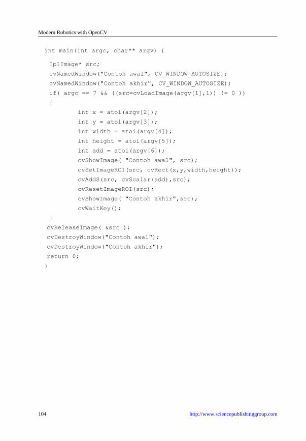
Modern Robotics with OpenCV
104 http://www.sciencepublishinggroup.com
int main(int argc, char** argv) {
IplImage* src;
cvNamedWindow("Contoh awal", CV_WINDOW_AUTOSIZE);
cvNamedWindow("Contoh akhir", CV_WINDOW_AUTOSIZE);
if( argc == 7 && ((src=cvLoadImage(argv[1],1)) != 0 ))
{
int x = atoi(argv[2]);
int y = atoi(argv[3]);
int width = atoi(argv[4]);
int height = atoi(argv[5]);
int add = atoi(argv[6]);
cvShowImage( "Contoh awal", src);
cvSetImageROI(src, cvRect(x,y,width,height));
cvAddS(src, cvScalar(add),src);
cvResetImageROI(src);
cvShowImage( "Contoh akhir",src);
cvWaitKey();
}
cvReleaseImage( &src );
cvDestroyWindow("Contoh awal");
cvDestroyWindow("Contoh akhir");
return 0;
}

Chapter 6 Introduction to OpenCV
http://www.sciencepublishinggroup.com 105
Figure 6.9 ROI of image.
Optical Flow
Optical flow or optic flow is the pattern of apparent motion of objects,
surfaces, and edges in a visual scene caused by the relative motion between an
observer (an eye or a camera) and the scene. calcOpticalFlowPyrLK calculates
an optical flow for a sparse feature set using the iterative Lucas-Kanade method
with pyramids.
OpticalFlow.cpp:
#include <opencv2/opencv.hpp>
#include <iostream>
#include <vector>
#include <cmath>
using namespace cv;
using namespace std;
int main(int argc, char** argv)
{

Modern Robotics with OpenCV
106 http://www.sciencepublishinggroup.com
// Load 2 image
Mat imgA = imread("left02.jpg", CV_LOAD_IMAGE_GRAYSCALE);
Mat imgB = imread("left03.jpg", CV_LOAD_IMAGE_GRAYSCALE);
Size img_sz = imgA.size();
Mat imgC(img_sz,1);
int win_size = 15;
int maxCorners = 20;
double qualityLevel = 0.05;
double minDistance = 5.0;
int blockSize = 3;
double k = 0.04;
std::vector<cv::Point2f> cornersA;
cornersA.reserve(maxCorners);
std::vector<cv::Point2f> cornersB;
cornersB.reserve(maxCorners);
goodFeaturesToTrack( imgA,cornersA,maxCorners,qualityLevel,minD
istance,cv::Mat());
goodFeaturesToTrack( imgB,cornersB,maxCorners,qualityLevel,minD
istance,cv::Mat());
cornerSubPix( imgA, cornersA, Size( win_size, win_size ),
Size( -1, -1 ),
TermCriteria( CV_TERMCRIT_ITER | CV_TERMCRIT_EPS, 20, 0.03 ) );
cornerSubPix( imgB, cornersB, Size( win_size, win_size ),
Size( -1, -1 ),
TermCriteria( CV_TERMCRIT_ITER | CV_TERMCRIT_EPS, 20, 0.03 ) );
// Call Lucas Kanade algorithm
CvSize pyr_sz = Size( img_sz.width+8, img_sz.height/3 );
std::vector<uchar> features_found;
features_found.reserve(maxCorners);
std::vector<float> feature_errors;
feature_errors.reserve(maxCorners);
calcOpticalFlowPyrLK( imgA, imgB, cornersA, cornersB,
features_found, feature_errors ,
Size( win_size, win_size ), 5,

Chapter 6 Introduction to OpenCV
http://www.sciencepublishinggroup.com 107
cvTermCriteria( CV_TERMCRIT_ITER | CV_TERMCRIT_EPS, 20, 0.3 ),
0 );
// Make an image of the results
for( int i=0; i < features_found.size(); i++ ){
cout<<"Error is "<<feature_errors[i]<<endl;
//continue;
cout<<"Got it"<<endl;
Point p0( ceil( cornersA[i].x ), ceil( cornersA[i].y ) );
Point p1( ceil( cornersB[i].x ), ceil( cornersB[i].y ) );
line( imgC, p0, p1, CV_RGB(255,255,255), 2 );
}
namedWindow( "ImageA", 0 );
namedWindow( "ImageB", 0 );
namedWindow( "LKpyr_OpticalFlow", 0 );
imshow( "ImageA", imgA );
imshow( "ImageB", imgB );
imshow( "LKpyr_OpticalFlow", imgC );
cvWaitKey(0);
return 0;
}
(a) (b) (c)
Figure 6.10 Result of optical flow program from 2 images.

Modern Robotics with OpenCV
108 http://www.sciencepublishinggroup.com
References
[1] Gary Bradski & Adrian Kaehler, Learning OpenCV (2008), O’Reilly Publisher.
[2] Robert Laganiere, OpenCV 2 Computer Vision Application Programming
Cookbook, 2011.
[3] Richard Szeliski, Computer Vision: Algorithms and Applications, 2010.
[4] Budiharto W., Santoso A., Purwanto D., Jazidie A., A Navigation System for
Service robot using Stereo Vision, 11th International conference on Control,
Automation and Systems, Kyntext-Korea, pp 101-107, 2011.

Chapter 7
Programming OpenCV


http://www.sciencepublishinggroup.com 111
On successful completion of this course, students will be able to:
Explain the morphological filtering.
Explain MeanShift and CamShift algorithms.
Develop a program to tracking an object using MeanShift() and
CamShift().
Introduction
Morphological filtering is a theory developed in the 1960s for the analysis
and processing of discrete images. It defines a series of operators which
transform an image by probing it with a predefined shape element. The way this
shape element intersects the neighborhood of a pixel determines the result of the
operation. Tracking an object is important features for intelligent robotics.
Meansift is an algorithm that finds an object in a backprjected histograma image.
Camshift is a histogram backprojection-based object tracking algorithm that
uses meanshift at its heart. It takes the detection window output by meanshift
and figures out the best size and rotation of that window to track the object.
Morphological Filtering
As morphological filters usually work on binary images, we will use a binary
image produced through thresholding. However, since in morphology, the
convention is to have foreground objects represented by high (white) pixel
values and background by low (black) pixel values, we have negated the image.
Morphological operations are a set of operations that process images based on
shapes. Morphological operations apply a structuring element to an input image
and generate an output image. The most basic morphological operations are two:
Erosion and Dilation. They have a wide array of uses, i.e.:
Removing noise.
Isolation of individual elements and joining disparate elements in an image.
Finding of intensity bumps or holes in an image.
Erosion and dilation are implemented in OpenCV as simple functions which
are cv::erode and cv::dilate. The opening and closing filters are simply defined

Modern Robotics with OpenCV
112 http://www.sciencepublishinggroup.com
in terms of the basic erosion and dilation operations. Closing is defined as the
erosion of the dilation of an image, and Opening is defined as the dilation of the
erosion of an image. The code below show an example of erotion and dilation:
Morphology.cpp:
#include "opencv2/imgproc/imgproc.hpp"
#include "opencv2/highgui/highgui.hpp"
#include "highgui.h"
#include <stdlib.h>
#include <stdio.h>
using namespace cv;
/// Global variables
Mat src, erosion_dst, dilation_dst;
int erosion_elem = 0;
int erosion_size = 0;
int dilation_elem = 0;
int dilation_size = 0;
int const max_elem = 2;
int const max_kernel_size = 21;
/** Function Headers */
void Erosion( int, void* );
void Dilation( int, void* );
int main( int argc, char** argv )
{
/// Load an image
// src = imread( argv[1] ); // if using command prompt
src = imread("flower.jpg");
if( !src.data )
{ return -1; }
/// Create windows
namedWindow( "Erosion Demo", CV_WINDOW_AUTOSIZE );
namedWindow( "Dilation Demo", CV_WINDOW_AUTOSIZE );
cvMoveWindow( "Dilation Demo", src.cols, 0 );

Chapter 7 Programming OpenCV
http://www.sciencepublishinggroup.com 113
/// Create Erosion Trackbar
createTrackbar( "Element:\n 0: Rect \n 1: Cross \n 2: Ellipse",
"Erosion Demo",
&erosion_elem, max_elem,
Erosion );
createTrackbar( "Kernel size:\n 2n +1", "Erosion Demo",
&erosion_size, max_kernel_size,
Erosion );
/// Create Dilation Trackbar
createTrackbar( "Element:\n 0: Rect \n 1: Cross \n 2: Ellipse",
"Dilation Demo",
&dilation_elem, max_elem,
Dilation );
createTrackbar( "Kernel size:\n 2n +1", "Dilation Demo",
&dilation_size, max_kernel_size,
Dilation );
/// Default start
Erosion( 0, 0 );
Dilation( 0, 0 );
waitKey(0);
return 0;
}
void Erosion( int, void* )
{
int erosion_type;
if( erosion_elem == 0 ){ erosion_type = MORPH_RECT; }
else if( erosion_elem == 1 ){ erosion_type = MORPH_CROSS; }
else if( erosion_elem == 2) { erosion_type = MORPH_ELLIPSE; }
Mat element = getStructuringElement( erosion_type,
Size( 2*erosion_size + 1, 2*erosion_size+1 ),
Point( erosion_size, erosion_size ) );
/// Apply the erosion operation
erode( src, erosion_dst, element );

Modern Robotics with OpenCV
114 http://www.sciencepublishinggroup.com
imshow( "Erosion Demo", erosion_dst );
}
void Dilation( int, void* )
{
int dilation_type;
if( dilation_elem == 0 ){ dilation_type = MORPH_RECT; }
else if( dilation_elem == 1 ){ dilation_type = MORPH_CROSS; }
else if( dilation_elem == 2) { dilation_type = MORPH_ELLIPSE; }
Mat element = getStructuringElement( dilation_type,
Size( 2*dilation_size + 1, 2*dilation_size+1 ),
Point( dilation_size, dilation_size ) );
/// Apply the dilation operation
dilate( src, dilation_dst, element );
imshow( "Dilation Demo", dilation_dst );
}
Figure 7.1 result of erotion and dilation.

Chapter 7 Programming OpenCV
http://www.sciencepublishinggroup.com 115
Camshift for Tracking Object
Meansift is an algorithm that finds an object in a backprjected histogram
image. Camshift is a histogram backprojection-based object tracking algorithm
that uses meanshift at its heart. It takes the detection window output by
meanshift and figures out the best size and rotation of that window to track the
object. OpenCV fuctions meanShift() and CamShift() implement these
algorithm.
Camshift.cpp:
#include "stdafx.h"
#include "opencv2/video/tracking.hpp"
#include "opencv2/imgproc/imgproc.hpp"
#include "opencv2/highgui/highgui.hpp"
#include <iostream>
#include <ctype.h>
using namespace cv;
using namespace std;
Mat image;
bool backprojMode = false;
bool selectObject = false;
int trackObject = 0;
bool showHist = true;
Point origin;
Rect selection;
int vmin = 10, vmax = 256, smin = 30;
static void onMouse( int event, int x, int y, int, void* )
{
if( selectObject )
{
selection.x = MIN(x, origin.x);
selection.y = MIN(y, origin.y);
selection.width = std::abs(x - origin.x);
selection.height = std::abs(y - origin.y);

Modern Robotics with OpenCV
116 http://www.sciencepublishinggroup.com
selection &= Rect(0, 0, image.cols, image.rows);
}
switch( event )
{
case CV_EVENT_LBUTTONDOWN:
origin = Point(x,y);
selection = Rect(x,y,0,0);
selectObject = true;
break;
case CV_EVENT_LBUTTONUP:
selectObject = false;
if( selection.width > 0 && selection.height > 0 )
trackObject = -1;
break;
}
}
const char* keys =
{
"{1| | 0 | camera number}"
};
int main( int argc, const char** argv )
{
VideoCapture cap;
Rect trackWindow;
int hsize = 16;
float hranges[] = {0,180};
const float* phranges = hranges;
CommandLineParser parser(argc, argv, keys);
int camNum = parser.get<int>("1");
cap.open(camNum);
IplImage img = image;
if( !cap.isOpened() )
{

Chapter 7 Programming OpenCV
http://www.sciencepublishinggroup.com 117
cout << "***Could not initialize capturing...***\n";
parser.printParams();
return -1;
}
namedWindow( "Histogram", 0 );
namedWindow( "VISION-BASED GRASPING FOR ARM ROBOT", 0 );
setMouseCallback("VISION-BASED GRASPING FOR ARM ROBOT",
onMouse, 0 );
createTrackbar( "Vmin", "VISION-BASED GRASPING FOR ARM ROBOT",
&vmin, 256, 0 );
createTrackbar( "Vmax", "VISION-BASED GRASPING FOR ARM ROBOT",
&vmax, 256, 0 );
createTrackbar( "Smin", "VISION-BASED GRASPING FOR ARM ROBOT",
&smin, 256, 0 );
Mat frame, hsv, hue, mask, hist, histimg = Mat::zeros(200, 320,
CV_8UC3), backproj;
bool paused = false;
for(;;)
{
if( !paused )
{
cap >> frame;
if( frame.empty() )
break;
}
frame.copyTo(image);
if( !paused )
{
cvtColor(image, hsv, CV_BGR2HSV);
if( trackObject )
{
int _vmin = vmin, _vmax = vmax;
inRange(hsv, Scalar(0, smin, MIN(_vmin,_vmax)),
Scalar(180, 256, MAX(_vmin, _vmax)), mask);
int ch[] = {0, 0};

Modern Robotics with OpenCV
118 http://www.sciencepublishinggroup.com
hue.create(hsv.size(), hsv.depth());
mixChannels(&hsv, 1, &hue, 1, ch, 1);
if( trackObject < 0 )
{
Mat roi(hue, selection), maskroi(mask, selection);
calcHist(&roi, 1, 0, maskroi, hist, 1, &hsize, &phranges);
normalize(hist, hist, 0, 255, CV_MINMAX);
trackWindow = selection;
trackObject = 1;
histimg = Scalar::all(0);
int binW = histimg.cols / hsize;
Mat buf(1, hsize, CV_8UC3);
for( int i = 0; i < hsize; i++ )
buf.at<Vec3b>(i) =
Vec3b(saturate_cast<uchar>(i*180./hsize), 255, 255);
cvtColor(buf, buf, CV_HSV2BGR);
for( int i = 0; i < hsize; i++ )
{
int val =
saturate_cast<int>(hist.at<float>(i)*histimg.rows/255);
rectangle( histimg, Point(i*binW,histimg.rows),
Point((i+1)*binW,histimg.rows - val),
Scalar(buf.at<Vec3b>(i)), -1, 8 );
}
}
calcBackProject(&hue, 1, 0, hist, backproj, &phranges);
backproj &= mask;
RotatedRect trackBox = CamShift(backproj, trackWindow,
TermCriteria( CV_TERMCRIT_EPS | CV_TERMCRIT_ITER, 10,
1 ));
if( trackWindow.area() <= 1 )
{
int cols = backproj.cols, rows = backproj.rows, r =
(MIN(cols, rows) + 5)/6;
trackWindow = Rect(trackWindow.x - r, trackWindow.y - r,

Chapter 7 Programming OpenCV
http://www.sciencepublishinggroup.com 119
trackWindow.x + r, trackWindow.y + r) &
Rect(0, 0, cols, rows);
}
if( backprojMode )
cvtColor( backproj, image, CV_GRAY2BGR );
ellipse( image, trackBox, Scalar(0,0,255), 3, CV_AA );
// cvRectangle
(&image,cvPoint(trackBox.center),cvPoint(trackBox.center),CV_RGB(
255,0,0), 3);
//cvRectangle(&frame,
cvPoint(trackWindow.x,trackWindow.y),cvPoint(trackWindow.x+20,tra
ckWindow.y+20), CV_RGB(255,0,0), 3 );
}
}
else if( trackObject < 0 )
paused = false;
if( selectObject && selection.width > 0 && selection.height >
0 )
{
Mat roi(image, selection);
bitwise_not(roi, roi);
}
imshow( "VISION-BASED GRASPING FOR ARM ROBOT", image );
imshow( "Histogram", histimg );
char c = (char)waitKey(10);
if( c == 27 )
break;
switch(c)
{
case 'b':
backprojMode = !backprojMode;
break;
case 'c':
trackObject = 0;
histimg = Scalar::all(0);
Modern Robotics with OpenCV
120 http://www.sciencepublishinggroup.com
break;
case 'h':
showHist = !showHist;
if( !showHist )
destroyWindow( "Histogram" );
else
namedWindow( "Histogram", 1 );
break;
case 'p':
paused = !paused;
break;
default:
;
}
}
return 0;
}

Chapter 7 Programming OpenCV
http://www.sciencepublishinggroup.com 121
Figure 7.2 Result of object detection.

Modern Robotics with OpenCV
122 http://www.sciencepublishinggroup.com
References
[1] Adrian Kaehler & Garry Bradksy, Learning OpenCV: Computer Vision in C++
with the OpenCV Library, O'Reilly PUblisher, 2014.
[2] Samarth Brahmbatt, Practical OpenCV, Technology in Action Publisher, 2013.
[3] Daniel bagio et al., Mastering OpenCV with Practical Computer Vision
Project, Packt Publisher, 2012.

Chapter 8
Extracting the Component’s Contours
for Calculating Number of Objects


http://www.sciencepublishinggroup.com 125
On successful completion of this course, students will be able to:
Explain how to extract component’s contours.
Develop a program to count an object in image.
Introduction
Image processing for obtaining object‘s information in an image is important
part in digital era. Important images generally contain representation of specific
objects. In order to perform a content-based analysis of an image, it is necessary
to extract meaningful features from the collection of pixels and contours that
constitute the image. Contours are fundamental image elements that define an
image’s content. In this paper, we propose a method for calculating number of
objects using computer vision based on contours and shape descriptor of image.
Introduction of Contours
Images generally contain representation of objects. One of the goals of image
analysis is to identify and extract those objects. In object detection/recognition
applications, the first step is to produce a binary image showing where certain
objects of interest could be located. The next step is to then extract the objects
which are contain in this collection of 1s and 0s. More specifically, we will
extract the connected components, that is, shapes made of a set of connected
pixels in a binary image. In this paper, we propose a method for calculating
objects in an image using contour and shape descriptor. The implementation of
this method is such as to get information about traffic density, how many cars in
a street.
The contours are extracted by a simple algorithm that consists of
systematically scanning the image until a component is hit. From this starting
point of the component, its contour is followed, marking the pixels on its border.
When the contour is completed, the scanning resumes at the last position until a
new component is found. The identified connected components can then be
individually analyzed. Implementation of image segmentation for extracting
foreground object can be use GraphCut algorithm based on mathematical
morphology [3]. GrabCut is computationally more expensive than watershed,
but it generally produces a more accurate result. It is the best algorithm to use

Modern Robotics with OpenCV
126 http://www.sciencepublishinggroup.com
when one wants to extract a foreground object in a still image. So for this
research, we propose simple mechanism for calculating the objects in an image,
by processing the contour and the shape descriptor of an image using connected
component.
Shape descriptors are important tools in content-based image retrieval
systems, which allow searching and browsing images in a database with respect
to the shape information. The shape description methods can be divided into
three main categories; contour based, image based and skeleton based
descriptors [5]. A Connected component often corresponds to the image of
some object in a pictured scene. To identify this object, or to compare it with
other image elements, it can be useful to perform some measurements on the
component in order to extract some of its characteristics. Many OpenCV functions are available when it comes to shape descriptor and offers a simple
function which extracts the contours of the connected components of an image
using cv::findContours function.
Cv::findCounteours (image,
CV_RETR_EXTERNAL, //retrieve the external contours
CV_CHAIN_APROX_NONE); // all pixels of each contours.
For example, if some prior knowledge is available about the expected size of
objects of interest, it becomes possible to eliminate some of the components.
Let’s then use a minimum and a maximum value for the perimeter of the
components by iterating over the vector of contours and eliminating the
eliminating the invalid components. The implementation for finding contours
shown in the program below:
// Eliminate too short or too long contours
intcmin=100;int cmax=1000 //min and max contour length
std::vector<std::vector<cv::Point>>::
const_iteratoritc=contours.begin();
while (itc !=contours.end()) {
if (itc->size()<cmin ||itc->size() >cmax)
itc=contour//Eliminate.erase(itc);
else
++itc;
}

Chapter 8 Extracting the Component’s Contours for Calculating Number of Objects
http://www.sciencepublishinggroup.com 127
Counting Objects
We using singe images for the experiment, and convert it first to binary, then
we extract the contour, shape descriptor, counting and displaying number of
objects. The algorithm for extract the contours shown below:
Algorithm 8.1. Extracting the contour and counting the object:
Begin
Counter=0
reading image and convert to binary image
Extract contours
Output the vector of contours
Counting the objects
Couter+=1
Displaying the number of object
End
The diagram block of our method shown in figure 8.1:
Figure 8.1 Diagram block of the system for calculating number of objects.
We test an example image with 4 animal and size 400x600 pixel as shown in
figure 8.2:

Modern Robotics with OpenCV
128 http://www.sciencepublishinggroup.com
Figure 8.2 Testing image.
Then the result of binary image from fig. 8.2 shown in figure 8.3:
Figure 8.3 Binary image.
After that, we find contours of image as shown in figure 8.4:

Chapter 8 Extracting the Component’s Contours for Calculating Number of Objects
http://www.sciencepublishinggroup.com 129
Figure 8.4 Contour of image obtained.
After that, we got total number of object with its shape descriptors as shown
in figure 8.5, using function:
CvPoint pt1;
pt1.x=100;pt1.y=60;
cvInitFont( &font, CV_FONT_HERSHEY_COMPLEX, 0.5, 0.5,
0.0, 1, CV_AA );
cvPutText( img, "TOTAL :", varCount, &font ,
CV_RGB(0,0,255) );

Modern Robotics with OpenCV
130 http://www.sciencepublishinggroup.com
Figure 8.5 Number of objects obtained with processing time less than 1 second.
References
[1] Robert Laganière, OpenCV 2 Computer Vision Application Programming
Cookbook, Apress Publisher, 2011.
[2] R.C. Gonzalez, Digital Image Processing (3rd
ed.), Addison Wesley, 2007.
[3] Rother, A Blake, GrabCut: Interactive Foreground Extraction using Iterated Graph
Cuts, ACM Transaction on Graphics, vol. 23 no. 3, 2004.
[4] R. Szeliski, Computer Vision, Algorithms and Applications, Springer Publisher,
2011.
[5] Latecki, L. J., Lakamper, R., Shape Similarity Measure Based on Correspondence
of Visual Parts.IEEE Transaction. PAMI, 22, 10, pp.1185-1190, 2000.

Chapter 9
Face Recognition Systems


http://www.sciencepublishinggroup.com 133
On successful completion of this course, students will be able to:
Explain how to detect face in OpenCV.
Develop face recognition systems using library in OpenCV.
Introduction
The face is our primary focus of attention in developing an iintelligent robot
to serves peoples. Unfortunatelly, developing a computational model of face
recognition is quite difficult, because faces are complex, meaningful visual
stimuli and multidimensional. Modelling of face images can be based on
statistical model such as Principal Component Analysis (PCA) and Linear
Discriminant analysis (LDA)and physical modelling based on the assumption of
certain surface reflectance properties, such as Lambertian surface. OpenCV
provides functions for face detector using Paul Viola and Michael Jones method,
and OpenCV facetracker using Camshift algorithm.
Face Recognition in OpenCV
Face recognition is an easy task for humans, but not for computer systems.
All face recognition models in OpenCV 2.4 are derived from the abstract base
class FaceRecognizer, which provides a unified access to all face recongition
algorithms in OpenCV. The currently available algorithms are:
Eigenfaces (see createEigenFaceRecognizer())
Fisherfaces (see createFisherFaceRecognizer())
Local Binary Patterns Histograms (see createLBPHFaceRecognizer())
Experiments in [16] have shown, that even one to three day old babies are
able to distinguish between known faces. So how hard could it be for a
computer? It turns out we know little about human recognition to date. Are
inner features (eyes, nose, mouth) or outer features (head shape, hairline) used
for a successful face recognition? How do we analyze an image and how does
the brain encode it? It was shown by David Hubel and Torsten Wiesel, that our
brain has specialized nerve cells responding to specific local features of a scene,
such as lines, edges, angles or movement. Since we don’t see the world as
scattered pieces, our visual cortex must somehow combine the different sources

Modern Robotics with OpenCV
134 http://www.sciencepublishinggroup.com
of information into useful patterns. Automatic face recognition is all about
extracting those meaningful features from an image, putting them into a useful
representation and performing some kind of classification on them.
Face recognition based on the geometric features of a face is probably the
most intuitive approach to face recognition. One of the first automated face
recognition systems was described by Kanade in 1973, marker points (position
of eyes, ears and nose) were used to build a feature vector (distance between
the points, angle between them). The recognition was performed by calculating
the euclidean distance between feature vectors of a probe and reference image.
The Eigenfaces method described in [15] took a holistic approach to face
recognition: A facial image is a point from a high-dimensional image space and
a lower-dimensional representation is found, where classification becomes easy.
The lower-dimensional subspace is found with Principal Component Analysis,
which identifies the axes with maximum variance. While this kind of
transformation is optimal from a reconstruction standpoint, it doesn’t take any
class labels into account. Imagine a situation where the variance is generated
from external sources, let it be light. The axes with maximum variance do not
necessarily contain any discriminative information at all, hence a classification
becomes impossible. So a class-specific projection with a Linear Discriminant
Analysis was applied to face recognition in [17]. The basic idea is to minimize
the variance within a class, while maximizing the variance between the classes
at the same time.
Recently various methods for a local feature extraction emerged. To avoid the
high-dimensionality of the input data only local regions of an image are
described, the extracted features are (hopefully) more robust against partial
occlusion, illumation and small sample size. Algorithms used for a local feature
extraction are Gabor Wavelets [18], Discrete Cosinus Transform [19] and Local
Binary Patterns [20]. It’s still an open research question what’s the best way to
preserve spatial information when applying a local feature extraction, because
spatial information is potentially useful information.
The problem with the image representation we are given is its high
dimensionality. The Principal Component Analysis (PCA), which is the core of
the Eigenfaces method, finds a linear combination of features that maximizes
the total variance in data. While this is clearly a powerful way to represent data,
it doesn’t consider any classes and so a lot of discriminative information may be
lost when throwing components away. Imagine a situation where the variance in
your data is generated by an external source, let it be the light. The components

Chapter 9 Face Recognition Systems
http://www.sciencepublishinggroup.com 135
identified by a PCA do not necessarily contain any discriminative information
at all, so the projected samples are smeared together and a classification
becomes impossible.
The Linear Discriminant Analysis performs a class-specific dimensionality
reduction and was invented by the great statistician Sir R. A. Fisher. In order to
find the combination of features that separates best between classes the Linear
Discriminant Analysis maximizes the ratio of between-classes to within-classes
scatter, instead of maximizing the overall scatter. The idea is simple: same
classes should cluster tightly together, while different classes are as far away as
possible from each other in the lower-dimensional representation. This was also
recognized by Belhumeur, Hespanha and Kriegman and so they applied a
Discriminant Analysis to face recognition [22].
Haar Cascade Classifier
Viola-Jones framework has been widely used by researchers in order to
detect the location of faces and objects in a given image. Face detection
classifiers are shared by public communities, such as OpenCV [1]. Haar
Cascade Classifier use AdaBoost at every node in cascade to study high
detection level with multi-tree classifier rejection level at every node in cascade.
This algorithm combines some innovative features, such as:
1) Use haar-like input feature, threshold that is used to sum and differentiate
square regions from image.
2) Integral image technique that enable fast computation for square regions
or regions that is rotated 45 degree. This data structure is used to make
computation from Haar-like input feature faster.
3) Statistical Boosting to make binary node classification (yes/no) that
characterized with high detection level and weak rejection level.
4) Organizing weak classifier nodes from a rejection cascade. In other words,
first group from the classifiers is selected so best detection in image
region consist of an object although enabling many mistakes in detection;
the next classifier groups are the second best detection with weak level
rejection; and so on. In testing, an object can be known if that object
makes it through all cascades [2]. Haar-like input feature that are used by
classifier are:

Modern Robotics with OpenCV
136 http://www.sciencepublishinggroup.com
Figure 9.1 Haar-like input feature that are used by classifiers [2].
You have to inform to classifier, the directory to be used, such as
haarcascade_frontalface_default.xml. At OpenCV, stored on:
Program_Files/OpenCV/data/haarcasades/haarcascade_frontalface_d
efault.xml.
To running the detector for face and eyes, you have to call detectMultiScale()
that consist of 7 parameter:
//-- Detect faces
face_cascade.detectMultiScale (frame_gray, faces, 1.1, 2, 0,
Size(80, 80) );
for( int i = 0; i < faces.size(); i++ )
{
Mat faceROI = frame_gray (faces[i]);
std::vector<Rect> eyes;
//-- In each face, detect eyes
eyes_cascade.detectMultiScale (faceROI, eyes, 1.1, 2, 0
|CV_HAAR_SCALE_IMAGE, Size(30, 30) );
Program below show the demo to detect face and eyes using webcam:

Chapter 9 Face Recognition Systems
http://www.sciencepublishinggroup.com 137
HaarDetection.cpp
//Face and eyes detection using Haar Cascade Classifier
#include "opencv2/objdetect/objdetect.hpp"
#include "opencv2/highgui/highgui.hpp"
#include "opencv2/imgproc/imgproc.hpp"
#include <iostream>
using namespace std;
using namespace cv;
/** Function Headers */
void detectAndDisplay( Mat frame );
/** Global variables */
String face_cascade_name = "lbpcascade_frontalface.xml";
String eyes_cascade_name =
"haarcascade_eye_tree_eyeglasses.xml";
CascadeClassifier face_cascade;
CascadeClassifier eyes_cascade;
string window_name = "Face detection";
int main( int argc, const char** argv )
{
CvCapture* capture;
Mat frame;
//-- 1. Load the cascade
if( !face_cascade.load( face_cascade_name ) ){ printf("--
(!)Error loading face\n"); return -1; };
if( !eyes_cascade.load( eyes_cascade_name ) ){ printf("--
(!)Error loading eye\n"); return -1; };
//-- 2. Read the video stream
capture = cvCaptureFromCAM(0);
if( capture )
{
while( true )
{
frame = cvQueryFrame( capture );
//-- 3. Apply the classifier to the frame

Modern Robotics with OpenCV
138 http://www.sciencepublishinggroup.com
if( !frame.empty() )
{ detectAndDisplay( frame ); }
else
{ printf(" --(!) No captured frame -- Break!"); break; }
int c = waitKey(10);
if( (char)c == 'c' ) { break; }
}
}
return 0;
}
/**
* @function detectAndDisplay
*/
void detectAndDisplay( Mat frame )
{
std::vector<Rect> faces;
Mat frame_gray;
cvtColor( frame, frame_gray, CV_BGR2GRAY );
equalizeHist( frame_gray, frame_gray );
//-- Detect faces
face_cascade.detectMultiScale( frame_gray, faces, 1.1, 2, 0,
Size(80, 80) );
for( int i = 0; i < faces.size(); i++ )
{
Mat faceROI = frame_gray( faces[i] );
std::vector<Rect> eyes;
//-- In each face, detect eyes
eyes_cascade.detectMultiScale( faceROI, eyes, 1.1, 2, 0
|CV_HAAR_SCALE_IMAGE, Size(30, 30) );
if( eyes.size() == 2)
{
//-- Draw the face
Point center( faces[i].x + faces[i].width*0.5, faces[i].y +
faces[i].height*0.5 );

Chapter 9 Face Recognition Systems
http://www.sciencepublishinggroup.com 139
ellipse( frame, center, Size( faces[i].width*0.5,
faces[i].height*0.5), 0, 0, 360, Scalar( 255, 0, 0 ), 2, 8, 0 );
for( int j = 0; j < eyes.size(); j++ )
{ //-- Draw the eyes
Point center( faces[i].x + eyes[j].x + eyes[j].width*0.5,
faces[i].y + eyes[j].y + eyes[j].height*0.5 );
int radius = cvRound( (eyes[j].width +
eyes[j].height)*0.25 );
circle( frame, center, radius, Scalar( 255, 0, 255 ), 3, 8,
0 );
}
}
}
//-- Show the result
imshow( window_name, frame );
}
The result of the program show in figure 9.2:
Figure 9.2 Result of face detection using Haar classifier.

Modern Robotics with OpenCV
140 http://www.sciencepublishinggroup.com
Displaying face detected from webcam with ellipse and rectangle usually
need by robotics engineer, because it can be used to measure distance between
camera and the object, the rectangle codes:
cvCircle( img, center, radius, color, 3, 8, 0 );
cvRectangle( img,cvPoint( r->x, r->y ),cvPoint( r->x + r-
>width, r->y + r->height ),CV_RGB( 0, 255, 0 ), 1, 8, 0 );
Program below show an example for face detection with rectangle:
Figure 9.3 Face detected using rectangle.
FaceRectangle.cpp:
//Face Detection using Rectangle
#include "stdafx.h"
#include "opencv2/objdetect/objdetect.hpp"
#include "opencv2/highgui/highgui.hpp"
#include "opencv2/imgproc/imgproc.hpp"
#include <iostream>
#include "cv.h"

Chapter 9 Face Recognition Systems
http://www.sciencepublishinggroup.com 141
#include "highgui.h"
#include <iostream>
#include <cstdio>
#ifdef _EiC
#define WIN32
#endif
using namespace std;
using namespace cv;
void detectAndDraw( Mat& img,
CascadeClassifier& cascade, CascadeClassifier&
nestedCascade,
double scale);
String cascadeName ="haarcascade_frontalface_alt.xml";
int main( int argc, const char** argv )
{
CvCapture* capture = 0;
Mat frame, frameCopy, image;
const String scaleOpt = "--scale=";
size_t scaleOptLen = scaleOpt.length();
const String cascadeOpt = "--cascade=";
size_t cascadeOptLen = cascadeOpt.length();
String inputName;
CascadeClassifier cascade, nestedCascade;
double scale = 1;
if( !cascade.load( cascadeName ) )
{
cerr << "ERROR: Could not load classifier cascade" << endl;
cerr << "Usage: facedetect [--cascade=\"<cascade_path>\"]\n"
" [--nested-cascade[=\"nested_cascade_path\"]]\n"
" [--scale[=<image scale>\n"
" [filename|camera_index]\n" ;
return -1;
}

Modern Robotics with OpenCV
142 http://www.sciencepublishinggroup.com
capture = cvCaptureFromCAM(0);
cvNamedWindow( "Face Detection with Rectangle", 1 );
if( capture )
{
for(;;)
{
IplImage* iplImg = cvQueryFrame( capture );
frame = iplImg;
if( frame.empty() )
break;
if( iplImg->origin == IPL_ORIGIN_TL )
frame.copyTo( frameCopy );
else
flip( frame, frameCopy, 0 );
detectAndDraw( frameCopy, cascade, nestedCascade, scale );
if( waitKey( 10 ) >= 0 )
goto _cleanup_;
}
waitKey(0);
_cleanup_:
cvReleaseCapture( &capture );
}
cvDestroyWindow("result");
return 0;
}
void detectAndDraw( Mat& img,
CascadeClassifier& cascade, CascadeClassifier&
nestedCascade,
double scale)
{
int i = 0;
double t = 0;
vector<Rect> faces;

Chapter 9 Face Recognition Systems
http://www.sciencepublishinggroup.com 143
const static Scalar colors[] = { CV_RGB(100,0,255),
CV_RGB(0,100,255),
CV_RGB(0,255,255),
CV_RGB(0,255,0),
CV_RGB(255,128,0),
CV_RGB(255,255,0),
CV_RGB(255,0,0),
CV_RGB(255,0,255)} ;
Mat gray, smallImg( cvRound (img.rows/scale),
cvRound(img.cols/scale), CV_8UC1 );
cvtColor( img, gray, CV_BGR2GRAY );
resize( gray, smallImg, smallImg.size(), 0, 0, INTER_LINEAR );
equalizeHist( smallImg, smallImg );
t = (double)cvGetTickCount();
cascade.detectMultiScale( smallImg, faces,
1.1, 2, 0
//|CV_HAAR_FIND_BIGGEST_OBJECT
//|CV_HAAR_DO_ROUGH_SEARCH
|CV_HAAR_SCALE_IMAGE
,
Size(30, 30) );
t = (double)cvGetTickCount() - t;
printf( "detection time = %g ms\n",
t/((double)cvGetTickFrequency()*1000.) );
for( vector<Rect>::const_iterator r = faces.begin(); r !=
faces.end(); r++, i++ )
{
Mat smallImgROI;
vector<Rect> nestedObjects;
Point center;
Scalar color = colors[i%8];
int radius;
center.x = cvRound((r->x + r->width*0.5)*scale);
center.y = cvRound((r->y + r->height*0.5)*scale);
radius = cvRound((r->width + r->height)*0.25*scale);
circle( img, center, radius, color, 3, 8, 0 );
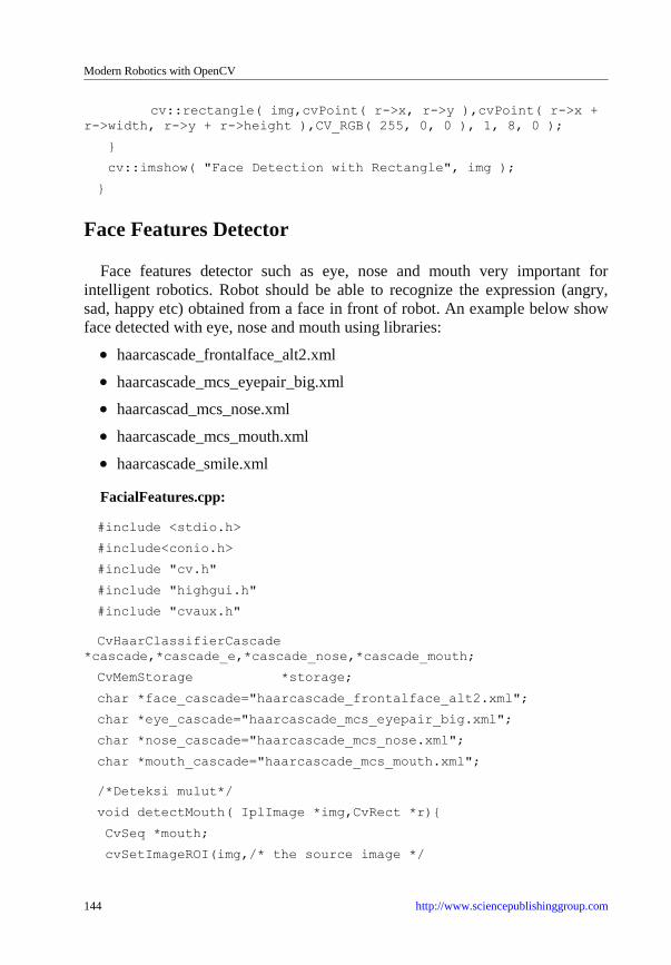
Modern Robotics with OpenCV
144 http://www.sciencepublishinggroup.com
cv::rectangle( img,cvPoint( r->x, r->y ),cvPoint( r->x +
r->width, r->y + r->height ),CV_RGB( 255, 0, 0 ), 1, 8, 0 );
}
cv::imshow( "Face Detection with Rectangle", img );
}
Face Features Detector
Face features detector such as eye, nose and mouth very important for
intelligent robotics. Robot should be able to recognize the expression (angry,
sad, happy etc) obtained from a face in front of robot. An example below show
face detected with eye, nose and mouth using libraries:
haarcascade_frontalface_alt2.xml
haarcascade_mcs_eyepair_big.xml
haarcascad_mcs_nose.xml
haarcascade_mcs_mouth.xml
haarcascade_smile.xml
FacialFeatures.cpp:
#include <stdio.h>
#include<conio.h>
#include "cv.h"
#include "highgui.h"
#include "cvaux.h"
CvHaarClassifierCascade
*cascade,*cascade_e,*cascade_nose,*cascade_mouth;
CvMemStorage *storage;
char *face_cascade="haarcascade_frontalface_alt2.xml";
char *eye_cascade="haarcascade_mcs_eyepair_big.xml";
char *nose_cascade="haarcascade_mcs_nose.xml";
char *mouth_cascade="haarcascade_mcs_mouth.xml";
/*Deteksi mulut*/
void detectMouth( IplImage *img,CvRect *r){
CvSeq *mouth;
cvSetImageROI(img,/* the source image */

Chapter 9 Face Recognition Systems
http://www.sciencepublishinggroup.com 145
cvRect(r->x, /* x = start from leftmost */
r->y+(r->height *2/3), /* y = a few pixels from the top */
r->width, /* width = same width with the face */
r->height/3 /* height = 1/3 of face height */
)
);
mouth = cvHaarDetectObjects(img,/* the source image, with the
estimated
location defined */
cascade_mouth, /* the eye classifier */
storage, /* memory buffer */
1.15, 4, 0, /* tune for your app */
cvSize(25, 15) /* minimum detection scale */
);
for( int i = 0; i < (mouth ? mouth->total : 0); i++ )
{
CvRect *mouth_cord = (CvRect*)cvGetSeqElem(mouth, i);
/* draw a red rectangle */
cvRectangle(img,
cvPoint(mouth_cord->x, mouth_cord->y),
cvPoint(mouth_cord->x + mouth_cord->width, mouth_cord->y +
mouth_cord->height),
CV_RGB(255,255, 255),
1, 8, 0
);
}
}
/*Deteksi hidung*/
void detectNose( IplImage *img,CvRect *r){
CvSeq *nose;
//nose detection- set ROI
cvSetImageROI(img, /* the source image */
cvRect(r->x, /* x = start from leftmost */
r->y, /* y = a few pixels from the top */
r->width, /* width = same width with the face */

Modern Robotics with OpenCV
146 http://www.sciencepublishinggroup.com
r->height /* height = 1/3 of face height */
)
);
nose = cvHaarDetectObjects(img, /* the source image, with the
estimated location defined */
cascade_nose, /* the eye classifier */
storage, /* memory buffer */
1.15, 3, 0, /* tune for your app */
cvSize(25, 15) /* minimum detection scale */
);
for( int i = 0; i < (nose ? nose->total : 0); i++ )
{
CvRect *nose_cord = (CvRect*)cvGetSeqElem(nose, i);
/* gambar kotak merah */
cvRectangle(img,
cvPoint(nose_cord->x, nose_cord->y),
cvPoint(nose_cord->x + nose_cord->width, nose_cord->y +
nose_cord->height),
CV_RGB(0,255, 0),
1, 8, 0
);
}
}
/*eye detection*/
void detectEyes( IplImage *img,CvRect *r){
char *eyecascade;
CvSeq *eyes;
int eye_detect=0;
/* Set the Region of Interest: estimate the eyes' position */
cvSetImageROI(img, /* the source image */
cvRect
(
r->x, /* x = start from leftmost */
r->y + (r->height/5.5), /* y = a few pixels from the top */

Chapter 9 Face Recognition Systems
http://www.sciencepublishinggroup.com 147
r->width, /* width = same width with the face */
r->height/3.0 /* height = 1/3 of face height */
)
);
/* deteksi mata */
eyes = cvHaarDetectObjects( img, /* the source image, with
the
estimated location defined */
cascade_e, /* the eye classifier */
storage, /* memory buffer */
1.15, 3, 0, /* tune for your app */
cvSize(25, 15) /* minimum detection scale */
);
printf("\n eye detected %d",eyes->total);
/* draw rectangle */
for( int i = 0; i < (eyes ? eyes->total : 0); i++ )
{
eye_detect++;
/* get one eye */
CvRect *eye = (CvRect*)cvGetSeqElem(eyes, i);
/* draw a red rectangle */
cvRectangle(img,
cvPoint(eye->x, eye->y),
cvPoint(eye->x + eye->width, eye->y + eye->height),
CV_RGB(0, 0, 255),
1, 8, 0
);
}
}
void detectFacialFeatures( IplImage *img,IplImage *temp_img,int
img_no){
char image[100],msg[100],temp_image[100];
float m[6];
double factor = 1;
CvMat M = cvMat( 2, 3, CV_32F, m );

Modern Robotics with OpenCV
148 http://www.sciencepublishinggroup.com
int w = (img)->width;
int h = (img)->height;
CvSeq* faces;
CvRect *r;
m[0] = (float)(factor*cos(0.0));
m[1] = (float)(factor*sin(0.0));
m[2] = w*0.5f;
m[3] = -m[1];
m[4] = m[0];
m[5] = h*0.5f;
cvGetQuadrangleSubPix(img, temp_img, &M);
CvMemStorage* storage=cvCreateMemStorage(0);
cvClearMemStorage( storage );
if( cascade )
faces = cvHaarDetectObjects(img,cascade, storage, 1.2, 2,
CV_HAAR_DO_CANNY_PRUNING, cvSize(20, 20));
else
printf("\nFrontal face cascade not loaded\n");
printf("\n Jumlah wajah yang dideteksi %d",faces->total);
/* for each face found, draw a red box */
for(int i = 0 ; i < ( faces ? faces->total : 0 ) ; i++ )
{
r = ( CvRect* )cvGetSeqElem( faces, i );
cvRectangle( img,cvPoint( r->x, r->y ),cvPoint( r->x + r-
>width, r->y + r->height ),
CV_RGB( 255, 0, 0 ), 1, 8, 0 );
printf("\n face_x=%d face_y=%d wd=%d ht=%d",r->x,r->y,r-
>width,r->height);
detectEyes(img,r);
/* reset region of interest */
cvResetImageROI(img);
detectNose(img,r);
cvResetImageROI(img);
detectMouth(img,r);

Chapter 9 Face Recognition Systems
http://www.sciencepublishinggroup.com 149
cvResetImageROI(img);
}
/* reset region of interest */
cvResetImageROI(img);
if(faces->total>0)
{
sprintf(image,"D:\\face_output\\%d.jpg",img_no);
cvSaveImage( image, img );
}
}
int main( int argc, char** argv )
{
CvCapture *capture;
IplImage *img,*temp_img;
Int key;
char image[100],temp_image[100];
storage = cvCreateMemStorage( 0 );
cascade = ( CvHaarClassifierCascade* )cvLoad( face_cascade, 0,
0, 0 );
cascade_e = ( CvHaarClassifierCascade* )cvLoad( eye_cascade, 0,
0, 0 );
cascade_nose = ( CvHaarClassifierCascade* )cvLoad( nose_cascade,
0, 0, 0 );
cascade_mouth =
( CvHaarClassifierCascade* )cvLoad( mouth_cascade, 0, 0, 0 );
if( !(cascade || cascade_e ||cascade_nose||cascade_mouth) )
{
fprintf( stderr, "ERROR: Could not load classifier
cascade\n" );
return -1;
}
for(int j=20;j<27;j++)
{
sprintf(image,"D:\\image\\%d.jpg",j);

Modern Robotics with OpenCV
150 http://www.sciencepublishinggroup.com
img=cvLoadImage(image);
temp_img=cvLoadImage(image);
if(!img)
{
printf("Could not load image file and trying once
again: %s\n",image);
}
printf("\n curr_image = %s",image);
detectFacialFeatures(img,temp_img,j);
}
cvReleaseHaarClassifierCascade( &cascade );
cvReleaseHaarClassifierCascade( &cascade_e );
cvReleaseHaarClassifierCascade( &cascade_nose );
cvReleaseHaarClassifierCascade( &cascade_mouth );
cvReleaseMemStorage( &storage );
cvReleaseImage(&img);
cvReleaseImage(&temp_img);
return 0;
}

Chapter 9 Face Recognition Systems
http://www.sciencepublishinggroup.com 151
Figure 9.4 Face features detected.
Face Recognition Systems
We have developed a framework for face recognition system and faces
database called ITS face database and will be compared with ATT and Indian
face database. The advantages of our framework is able to store ordered item
from customer in.xml file and displayed on the screen. In this research, we
construct images under different illumination conditions by generate a random
value for brightness level for ITS face database. Each of face database consists
of 10 sets of people’s face. Each set of ITS face database consists of 3 poses
(front, left, right ) and varied with illumination [13].

Modern Robotics with OpenCV
152 http://www.sciencepublishinggroup.com
Figure 9.5 ITS, Indian and ATT face database used as comparison to see the effect of
illumination at face recognition [13].
Rapid Object Detection with a Cascade of Boosted
Classifiers Based on Haar-like Features
To train and use a cascade of boosted classifiers for rapid object detection. A
large set of over-complete haar-like features provide the basis for the simple
individual classifiers. Examples of object detection tasks are face, eye and nose
detection, as well as logo detection. The sample detection task is logo detection,
since logo detection does not require the collection of large set of registered and
carefully marked object samples. For training a training samples must be
collected. There are two sample types: negative samples and positive samples.
Negative samples correspond to non-object images. Positive samples
correspond to object images.

Chapter 9 Face Recognition Systems
http://www.sciencepublishinggroup.com 153
Negative Samples
Negative samples are taken from arbitrary images. These images must not
contain object representations. Negative samples are passed through
background description file. It is a text file in which each text line contains the
filename (relative to the directory of the description file) of negative sample
image. This file must be created manually. Note that the negative samples and
sample images are also called background samples or background samples
images, and are used interchangeably in this document. Example of negative
description file:
/img
img1.jpg
img2.jpg
bg.txt
File bg.txt:
img/img1.jpg
img/img2.jpg
Positive Samples
Positive samples are created by createsamples utility. They may be created
from single object image or from collection of previously marked up images.
The single object image may for instance contain a company logo. Then are
large set of positive samples are created from the given object image by
randomly rotating, changing the logo color as well as placing the logo on
arbitrary background.
The amount and range of randomness can be controlled by command line
arguments.
Command line arguments:
- vec <vec_file_name>
name of the output file containing the positive samples for training
- img <image_file_name>
source object image (e.g., a company logo)
- bg <background_file_name>

Modern Robotics with OpenCV
154 http://www.sciencepublishinggroup.com
background description file; contains a list of images into which randomly
distorted versions of the object are pasted for positive sample generation
- num <number_of_samples>
number of positive samples to generate
- bgcolor <background_color>
background color (currently grayscale images are assumed); the background
color denotes the transparent color. Since there might be compression artifacts,
the amount of color tolerance can be specified by –bgthresh. All pixels between
bgcolor-bgthresh and bgcolor+bgthresh are regarded as transparent.
- bgthresh <background_color_threshold>
- inv
if specified, the colors will be inverted
- randinv
if specified, the colors will be inverted randomly
- maxidev <max_intensity_deviation>
maximal intensity deviation of foreground samples pixels
- maxxangle <max_x_rotation_angle>,
- maxyangle <max_y_rotation_angle>,
- maxzangle <max_z_rotation_angle>
maximum rotation angles in radians
-show
if specified, each sample will be shown. Pressing ‘Esc’ will continue creation
process without samples showing. Useful debugging option.
- w <sample_width>
width (in pixels) of the output samples
- h <sample_height>
height (in pixels) of the output samples

Chapter 9 Face Recognition Systems
http://www.sciencepublishinggroup.com 155
White noise is added to the intensities of the foreground. If –inv key is
specified then foreground pixel intensities are inverted. If –randinv key is
specified then it is randomly selected whether for this sample inversion will be
applied. Finally, the obtained image is placed onto arbitrary background from
the background description file, resized to the pixel size specified by –w and –h
and stored into the file specified by the –vec command line parameter. Positive
samples also may be obtained from a collection of previously marked up images.
This collection is described by text file similar to background description file.
Each line of this file corresponds to collection image. The first element of the
line is image file name. It is followed by number of object instances. The
following numbers are the coordinates of bounding rectangles (x, y, width,
height).
Example of description file:
Directory structure:
/img
img1.jpg
img2.jpg
info.dat
File info.dat:
img/img1.jpg 1 140 100 45 45
img/img2.jpg 2 100 200 50 50 50 30 25 25
Image img1.jpg contains single object instance with bounding rectangle (140,
100, 45, 45). Image img2.jpg contains two object instances.
In order to create positive samples from such collection –info argument
should be specified instead of –img:
- info <collection_file_name>
description file of marked up images collection
The scheme of sample creation in this case is as follows. The object instances
are taken from images. Then they are resized to samples size and stored in
output file. No distortion is applied, so the only affecting arguments are –w, -h,
-show and –num.

Modern Robotics with OpenCV
156 http://www.sciencepublishinggroup.com
Create samples utility may be used for examining samples stored in positive
samples file. In order to do this only –vec, –w and –h parameters should be
specified.
Note that for training, it does not matter how positive samples files are
generated. So the createsamples utility is only one way to collect/create a vector
file of positive samples.
Training
The next step after samples creation is training of classifier. It is performed
by the haartraining utility.
Command line arguments:
- data <dir_name>
directory name in which the trained classifier is stored
- vec <vec_file_name>
file name of positive sample file (created by trainingsamples utility or by any
other means)
- bg <background_file_name>
background description file
- npos <number_of_positive_samples>,
- nneg <number_of_negative_samples>
number of positive/negative samples used in training of each classifier stage.
Reasonable values are npos = 7000 and nneg = 3000.
- nstages <number_of_stages>
number of stages to be trained
- nsplits <number_of_splits>
determines the weak classifier used in stage classifiers. If 1, then a simple stump
classifier is used, if 2 and more, then CART classifier with number_of_splits
internal (split) nodes is used
- mem <memory_in_MB>

Chapter 9 Face Recognition Systems
http://www.sciencepublishinggroup.com 157
available memory in MB for precalculation. The more memory you have the
faster the training process
- sym (default),
- nonsym
specifies whether the object class under training has vertical symmetry or not.
Vertical symmetry speeds up training process. For instance, frontal faces show
off vertical symmetry
- minhitrate <min_hit_rate>
minimal desired hit rate for each stage classifier. Overall hit rate may be
estimated as (min_hit_rate^number_of_stages)
- maxfalsealarm <max_false_alarm_rate>
maximal desired false alarm rate for each stage classifier. Overall false alarm
rate may be estimated as (max_false_alarm_rate^number_of_stages)
- weighttrimming <weight_trimming>
Specifies wheter and how much weight trimming should be used. A decent
choice is 0.90.
- eqw
- mode <BASIC (default) | CORE | ALL>
selects the type of haar features set used in training. BASIC use only upright
features, while ALL uses the full set of upright and 45 degree rotated feature set.
See [1] for more details.
- w <sample_width>,
- h <sample_height>
Size of training samples (in pixels). Must have exactly the same values as used
during training samples creation (utility trainingsamples)
Note: in order to use multiprocessor advantage a compiler that supports
OpenMP 1.0 standard should be used. OpenCV cvHaarDetectObjects() function
(in particular haarFaceDetect demo) is used for detection.

Modern Robotics with OpenCV
158 http://www.sciencepublishinggroup.com
Test Samples
In order to evaluate the performance of trained classifier a collection of
marked up images is needed. When such collection is not available test samples
may be created from single object image by createsamplesutility. The scheme of
test samples creation in this case is similar to training samples creation since
each test sample is a background image into which a randomly distorted and
randomly scaled instance of the object picture is pasted at a random position. If
both –img and –info arguments are specified then test samples will be created
by createsamples utility. The sample image is arbitrary distorted as it was
described below, then it is placed at random location to background image and
stored. The corresponding description line is added to the file specified by –info
argument. The –w and –h keys determine the minimal size of placed object
picture.
The test image file name format is as follows:
imageOrderNumber_x_y_width_height.jpg,
where x, y, width and height are the coordinates of placed object bounding
rectangle.
Note that you should use a background images set different from the
background image set used during training. In order to evaluate the performance
of the classifier performance utility may be used. It takes a collection of marked
up images, applies the classifier and outputs the performance, i.e. number of
found objects, number of missed objects, number of false alarms and other
information.
Command line arguments:
- data <dir_name>
directory name in which the trained classifier is stored
- info <collection_file_name>
file with test samples description
- maxSizeDiff <max_size_difference>,
- maxPosDiff <max_position_difference>

Chapter 9 Face Recognition Systems
http://www.sciencepublishinggroup.com 159
determine the criterion of reference and detected rectangles coincidence.
Default values are 1.5 and 0.3 respectively.
- sf <scale_factor>,
detection parameter. Default value is 1.2.
- w <sample_width>,
- h <sample_height>
Size of training samples (in pixels). Must have exactly the same values as used
during training (utility haartraining).
Exercises
1) Create a program for smile detector using haarcascade_smile.xml.
2) Create a program for online face and Gender Recognition system using
fischerfaces and OpenCV.
Figure 9.6 Face and Gender Recognition Systems (improved from [21]).

Modern Robotics with OpenCV
160 http://www.sciencepublishinggroup.com
References
[1] Acosta, L., González, E.J., Rodríguez, J.N., Hamilton, A.F., Méndez J.A.,
Hernéndez S., Sigut S.M, and Marichal G.N. Design and Implementation of a
Service Robot for A Restaurant. International Journal of robotics and automation.
2006; vol. 21(4): pp. 273-281.
[2] Qing-wiau Y., Can Y., Zhuang F. and Yan-Zheng Z. Research of the Localization
of Restaurant Service Robot. International Journal of Advanced Robotic Systems.
2010; vol. 7(3): pp. 227-238.
[3] Chatib, O., Real-Time Obstacle Avoidance for Manipulators and Mobile Robots.,
The International Journal of Robotics Research, 1986; vol. 5(1), pp. 90-98.
[4] Borenstein, J., Koren, Y., The Vector Field Histogram- Fast Obstacle Avoidance
for Mobile Robots, in proc. IEEE Trans. On Robotics and Automation. 1991; vol
7(3): pp.278-288.
[5] S. Nuryono, Penerapan Multi Mikrokontroler pada Model Robot Mobil
Menggunakan Logika Fuzzy, Journal Telkomnika, 2009, vol. 7(3), pp, 213-218.
[6] Masehian E., Katebi Y. Robot Motion Planning in Dynamic Environments with
Moving Obstacles and Target. International Journal of Mechanical Systems
Science and Engineering. 2007; vol. 1(1), pp. 20-29.
[7] Budiharto, W., Purwanto, D. and Jazidie, A. A Robust Obstacle Avoidance for
Service Robot using Bayesian Approach. International Journal of Advanced
Robotic Systems. Intech Publisher – Austria. 2011; Vol. 8(1): pp. 52-60.
[8] Budiharto, W., Purwanto, D. & Jazidie, A. A Novel Method for Static and Moving
Obstacle Avoidance for Service robot using Bayesian Filtering. Proceeding of
IEEE 2nd International conf. on Advances in Computing, Control and
Telecommunications Technology.2010; pp. 156-160. DOI: 10.1109/ACT.2010.51.
[9] Purwanto, D. Visual Feedback Control in Multi-Degrees-of-Freedom Motion
System. PhD thesis at Graduate School of Science and Technology - Keio
University, Japan. 2001.
[10] Turk, M. & Pentland A. Eigenfaces for recognition. International Journal of
Cognitive Neuroscience. 1991; vol. 3(1): pp. 71-86.
[11] Belhumeur, P. & Kriegman, D. What is the set of images of an object under all
possible illumination conditions. International Journal of Computer Vision. 1998;
Vol. 28( 3), pp. 245-260.

Chapter 9 Face Recognition Systems
http://www.sciencepublishinggroup.com 161
[12] Etemad, K. & Chellappa R. Discriminant analysis for recognition of human face
images. Journal of the Optical Society of America A. 1997; vol. 14( 8): pp. 1724-
1733.
[13] Budiharto, W., Santoso A., Purwanto, D. and Jazidie, A. An Improved Face
recognition System for Service Robot using Stereo Vision. In: Tudor Barbu Editor.
Face Recognition / Book 3. Intech Publisher – Austria; 2011: pp. 1-12.
[14] Hu, H. & Brady, M. A Bayesian Approach to Real-Time Obstacle Avoidance for a
Mobile Robot. Autonomous Robots. 1994; vol. 1: pp. 69-92.
[15] Turk, M., and Pentland, A. Eigenfaces for recognition. Journal of Cognitive
Neuroscience 3 (1991), 71–86.
[16] Chiara Turati, Viola Macchi Cassia, F. S., and Leo, I. Newborns face recognition:
Role of inner and outer facial features. Child Development 77, 2 (2006), 297–311.
[17] Belhumeur, P. N., Hespanha, J., and Kriegman, D. Eigenfaces vs. Fisherfaces:
Recognition Using Class Specific Linear Projection. IEEE Transactions on Pattern
Analysis and Machine Intelligence 19, 7 (1997), 711–720.
[18] Wiskott, L., Fellous, J., Krüger, N., Malsburg, C. Face Recognition By Elastic
Bunch Graph Matching. IEEE Transactions on Pattern Analysis and Machine
Intelligence 19 (1997), S. 775–779.
[19] Messer, K. et al. Performance Characterisation of Face Recognition Algorithms
and Their Sensitivity to Severe Illumination Changes. In: In: ICB, 2006, S. 1–11.
[20] Ahonen, T., Hadid, A., and Pietikainen, M. Face Recognition with Local Binary
Patterns. Computer Vision - ECCV 2004 (2004), 469–481.
[21] Daniel Bagio et al, Mastering OpenCV with Practical Computer Vision Project,
Pact publisher, 2012.
[22] Opencv.org.


Chapter 10
Intelligent Humanoid Robot


http://www.sciencepublishinggroup.com 165
On successful completion of this course, students will be able to:
Explain how the humanoid robot works.
Develop vision-based humanoid robot.
Explain object detection using keypoints and feature matching.
Introduction
Modern Humanoid Robot in uncontrolled environments needs to be based on
vision and versatile. This paper propose a method for object measurement and
ball tracking method using Kalman Filter for Humanoid Soccer, because the
ability to accurately track a ball is one of the important features for processing
high-definition image. A color-based object detection is used for detecting a ball
while PID controller is used for controlling pan tilt camera system. We also
modify the robot’s controller CM-510 in order able to communicate efficiently
using main controller.
Humanoid Robot
The humanoid robot is popular nowadays for the entertainment or contests
such as RoboCup Humanoid League. The important features of humanoid
soccer, such as accuracy, robustness, efficient determination and tracking of ball
size and location; has proven to be a challenging subset of this task and the
focus of much research. With the evolution of robotics hardware and subsequent
advances in processor performance in recent years, the temporal and spatial
complexity of feature extraction algorithms to solve this task has grown (Ha et
al, 2011).
In the case of Humanoid soccer, vision systems are one of the main sources
for environment interpretation. Many problems have to be solved before having
a fully featured soccer player. First of all, the robot has to get information from
the environment, mainly using the camera. It must detect the ball, goals, lines
and the other robots. Having this information, the robot has to self-localize and
decide the next action: move, kick, search another object, etc. The robot must
perform all these tasks very fast in order to be reactive enough to be competitive
in a soccer match. It makes no sense within this environment to have a good
localization method if that takes several seconds to compute the robot position

Modern Robotics with OpenCV
166 http://www.sciencepublishinggroup.com
or to decide the next movement in few seconds based on the old perceptions
(Martin et al, 2011). At the same time many other topics like human-machine
interaction, robot cooperation and mission and behavior control give humanoid
robot soccer a higher level of complexity like no any other robots (Blanes et al,
2011). So the high speed processor with efficient algorithms is needed for this
issue.
One of the performance factors of a humanoid soccer is that it is highly
dependent on its tracking ball and motion ability. The vision module collects
information that will be the input for the reasoning module that involves the
development of behaviour control. Complexity of humanoid soccer makes
necessary playing with the development of complex behaviours, for example
situations of coordination or differ rent role assignment during the match. There
are many types of behaviour control, each with advantages and disadvantages:
reactive control is the simplest way to make the robot play, but do not permit
more elaborated strategies as explained for example in (Behnke, 2001). On the
other side, behaviour-based control are more complex but more difficult to
implement, and enables in general the possibility high-level behaviour control,
useful for showing very good performances. Intelligent tracking algorithm for
state estimation using Kalman filter has been successfully developed (Noh et al,
2007), and we want to implement that method for ball tracking for humanoid
soccer robot.
We propose architecture of low cost humanoid soccer robot compared with
the well known humanoid robots for education such as DarwIn-OP and NAO
and test its ability for image processing to measure distance of the ball and track
a ball using color-based object detection method, the robot will kick the ball
after getting the nearest position between the robot and the ball. The Kalman
filter is used here to estimate state variable of a ball that is excited by random
disturbances and measurement noise. It has good results in practice due to
optimality and structure and convenient form for online real time processing.
For future robotics, we will familiar with term of robot ethics. Robot ethics
is a growing interdisciplinary research effort roughly in the intersection of
applied ethics and robotics with the aim of understanding the ethical
implications and consequences of robotic technology. Swarm robotics is a new
approach to the coordination of multirobot systems which consist of large
numbers of mostly simple physical robots. It is supposed that a desired
collective behavior emerges from the interactions between the robots and
interactions of robots with the environment. Swarm robotics systems are

Chapter 10 Intelligent Humanoid Robot
http://www.sciencepublishinggroup.com 167
characterized by decentralized control, limited communication between robots,
and use of local information and emergence of global behavior.
The Architecture of the Humanoid Robot
Humanoid soccer robots design based on the vision involves the need to
obtain a mechanical structure with a human appearance, in order to operate into
a human real world. Another important feature for modern humanoid robot is
the ability to process tasks especially for computer vision. We propose an
embedded system that able to handle high speed image processing, so we use
main controller based on the ARM7 Processor. Webcam and servo controller
are used to track a ball, and the output of the main controller will communicate
with the CM510 controller to control the actuators and sensors of the robot as
shown in figure. 10.1.
Figure 10.1 Architecture of high speed system for Humanoid Soccer Robot.
The main controller uses Odroid X2 that consist of Cortext-A9 1.7 GHz and
sufficient memory and ports to be connected with other devices as shown in fig.
10.2. The specification of the Odroid X2:
Exynos4412 Quad-core ARM Cortex-A9 1.7GHz.
2GByte Memory.
6 x High speed USB2.0 Host port.
10/100Mbps Ethernet with RJ-45 LAN Jack.

Modern Robotics with OpenCV
168 http://www.sciencepublishinggroup.com
Figure 10.2 Odroid X2 for processing the images from webcam
(hardkernel.com, 2013).
The Firmware of the robot to control the servos is modified from the original
one named Robotis Firmware due to the limitation for sending a motion
command by serial interface based on Peter Lanius works published in google
code (Lanius, 2013). This firmware instead using RoboTask to program the
robot controlling its movement but it directly program the AVR Microcontroller
inside the CM-510 controller using C language. Using this alternative can
reduce the size of the program from originally 170KB to 70KB in the memory.
By this firmware, the robot can be connected directly to Ball Tracking System
using USB Serial Interface to command its motion. Based on this framework, it
opens an opportunity to built Real Time Operating System for the robot. The
robot’s control starts with initialization routines of CM-510 controller then
move to Wait for Start Button state. In this state, it waits the button to be
pressed to change the start_button_pressed variable from FALSE to TRUE then
move to Dynamixel and Gyro Initialization which send broadcast ping to every
Dynamixel servo connected to CM-510. When one or more servos do not
respond of the ping then CM-510 will send a message mentioning the failure of
a servo to serial terminal. Gyro Initialization does gyro calibration in the robot
to get center reference and sends the value to serial terminal. Next state is
Waiting Motion Command that waits the command through serial interface,
from terminal or tracking module, then check if the command is valid or not. If
it does not valid then the state will repeat to Wait Motion Command or continue

Chapter 10 Intelligent Humanoid Robot
http://www.sciencepublishinggroup.com 169
to next Execute Motion Command state when the command is valid. Execute
Motion Command executes a motion command to move a servos based on
defined Look-Up-Table (LUT).
For example, when a command says WALKING then the state looks servo’s
values for WALKING stored in the LUT then sends it to Dynamixel servo
through serial bus. When a motion is completed then it move to preceding state
but if there is an emergency which is determined by pressing start button when
the servos is moving compared to command input which does not receive stop
command, then it move to Dynamixel Torque Disable to disable all the servo’s
torque to save from damage and move to Wait for Start Button state. The
improved system to accept commands from the main controller is shown as the
state machine in figure 10.3.
Figure 10.3 State machine of the robot’s controller.

Modern Robotics with OpenCV
170 http://www.sciencepublishinggroup.com
Ball Distance Estimation and Tracking Algorithm
Computer vision is one of the most challenging applications in sensor
systems since the signal is complex from spatial and logical point of view. An
active camera tracking system for humanoid robot soccer tracks an object of
interest (ball) automatically with a pan-tilt camera. We use OpenCV for
converting to HSV (Hue Saturation-Value), extract Hue & Saturation and create
a mask matching only the selected range of hue value (Szeliski, 2010).
To have a good estimation, the object must be in the centre of the image, i.e.
it must be tracked. Once there, the distance and orientation are calculated,
according to the neck’s origin position, the current neck‘s servomotors position
and the position of the camera in respect to the origin resulting of the design
(Maggi, 2007). We considered method for distance estimation of the ball by
centering the ball on the camera image, using the head tilt angle to estimate the
distance to the ball.
Region growing algorithms are also used to locate the ball color blobs that
have been identified by region growing and are useful and robust source for
further image processing, as demonstrated by (Ghanai, 2009). The ball will be
tracked based on the color and webcam will track to adjust the position of the
ball to the center of the screen based on the Algorithm 1.
Algorithm 1: Ball tracking and Kick the ball
Get input image from the camera
Convert to HSV (Hue-Saturation-Value)
Extract Hue & Saturation
Create a mask matching only for the selected range of hue
Create a mask matching only for the selected saturation levels.
Find the position (moment) of the selected regions.
If ball detected then
Estimate distance of the ball
Object tracking using Kalman Filter
centering the position of the ball
Move robot to the ball
If ball at the nearest position with the robot then
Kick the ball
endif

Chapter 10 Intelligent Humanoid Robot
http://www.sciencepublishinggroup.com 171
endif
The estimated position , from Kalman filter is used as an input to PID
controller. We use a PID controller to calculate an error value as the difference
between a measured (input) and a desired set point to control high speed HS-85
servos. The controller attempts to minimize the error by adjusting (an Output).
The model of PID Controller is shown in figure 10. 4:
Figure 10.4 General PID Controller.
The output of a PID controller, equal to the control input to the system, in the
time-domain is as follows:
(10.1)
A Framework of Multiple Moving Obstacles Avoidance
Strategy
Because we want a general model for humanoid service robot, we propose a
framework for multiple moving obstacles avoidance strategy using stereo vision.
A multiple moving obstacle avoidance strategy is an important framework to
develop humanoid service robot in dynamic environment. There are two mains
actors on multiple moving obstacles avoidance system; the Robot itself and the
Range Finder. The Robot interacts with this system to detect customer and
determine moving obstacles. Both processes to detect customer and determine
moving obstacles include a process of face recognition as explained before.
After the obstacles are determined, The Range Finder (camera and its system)
will calculate and estimate the distance of those moving obstacles and estimate

Modern Robotics with OpenCV
172 http://www.sciencepublishinggroup.com
the direction of moving obstacles. Direction estimation of obstacles will be used
to determine optimal maneuver of the Robot to avoid those obstacles. The
framework is shown in figure 10.5:
Figure 10.5 The use case diagram for our multiple moving obstacles avoidance
strategy using stereo vision.
Visual perception is the ability to interpret the information and surroundings
from the effects of visible light reaching the eye. The resulting perception is
also known as eyesight, sight, or vision. Visual-perception-based of service
robot for customer identification is an interpretation process to direct a service
robot to a destination of identified customer based on face recognition system
and computer vision. After interpretation of images from camera done, then it is

Chapter 10 Intelligent Humanoid Robot
http://www.sciencepublishinggroup.com 173
used as information for the robot and to decide actions based on the task given
by a developer. The basic of visual–perception model for a humanoid service
robot is shown in figure 10.6:
Figure 10.6 Visual-perception model for vision-based humanoid robot. After
interpretation process, the information used for navigating the robot or deciding
actions for robot, such as direct a robot to customer’s position.
Experiments
Object detection and segmentation is the most important and challenging
fundamental task of computer vision. It is a critical part in many applications
such as image search, image auto-annotation and scene understanding. However
it is still an open problem due to the complexity of object classes and images.
The easiest way to detect and segment an object from an image is the color
based methods. The colors in the object and the background should have a
significant color difference in order to segment objects successfully using color
based methods.
We need a webcam to try detecting a ball using this program demo. Create an
application using Visual C++ 2010 Express edition and OpenCV. Configure the
properties and write a program below:
ColorBased.cpp:
//Demo Program of Color-Based Detection for a Ball
//Copyright Dr. Widodo Budiharto 2014
#include "stdafx.h"
#include <cv.h>
#include <highgui.h>
// threshold image HSV

Modern Robotics with OpenCV
174 http://www.sciencepublishinggroup.com
IplImage* GetThresholdedImage(IplImage* imgHSV){
IplImage*
imgThresh=cvCreateImage(cvGetSize(imgHSV),IPL_DEPTH_8U, 1);
cvInRangeS(imgHSV, cvScalar(170,160,60), cvScalar(180,256,256),
imgThresh);
return imgThresh;
}
int main(){
CvCapture* capture =0;
capture = cvCaptureFromCAM(0);
//set width and height
cvSetCaptureProperty( capture, CV_CAP_PROP_FRAME_WIDTH, 640 );
cvSetCaptureProperty( capture, CV_CAP_PROP_FRAME_HEIGHT, 480);
if(!capture){
printf("Capture failure\n");
return -1;
}
IplImage* frame=0;
cvNamedWindow("Video");
cvNamedWindow("Ball");
//iterasi frame
while(true){
frame = cvQueryFrame(capture);
if(!frame) break;
frame=cvCloneImage(frame);
//smooth the original image using Gaussian kernel
cvSmooth(frame, frame, CV_GAUSSIAN,3,3);
IplImage* imgHSV = cvCreateImage(cvGetSize(frame), IPL_DEPTH_8U,
3);
//ubah formwat color dari BGR ke HSV
cvCvtColor(frame, imgHSV, CV_BGR2HSV);
IplImage* imgThresh = GetThresholdedImage(imgHSV);
//smooth the binary image using Gaussian kernel
cvSmooth(imgThresh, imgThresh, CV_GAUSSIAN,3,3);
cvShowImage("Ball", imgThresh);

Chapter 10 Intelligent Humanoid Robot
http://www.sciencepublishinggroup.com 175
cvShowImage("Video", frame);
//bersihkan images
cvReleaseImage(&imgHSV);
cvReleaseImage(&imgThresh);
cvReleaseImage(&frame);
//tunggu 50sec
int c = cvWaitKey(10);
//If 'ESC' is pressed, break the loop
if((char)c==27 ) break;
}
cvDestroyAllWindows() ;
cvReleaseCapture(&capture);
return 0;
}
The approach proposed in this paper was implemented and tested on a
humanoid Robot named Humanoid Robot Soccer Ver 2.0 based on Bioloid
Premium Robot. By modify the robot’s controller (CM-510) in order to accept
serial command from the main controller, this system able to communicate
efficiently.

Modern Robotics with OpenCV
176 http://www.sciencepublishinggroup.com
Figure 10.7 The original image (a), the mask (a) and ball detected and tracked using
Kalman Filters in the green circle (b).
When a ball is in front of the robot and has been detected, the robot tries to
track the ball, and if the ball at the nearest position with the robot, robot will
kick it as shown in figure 10.8.

Chapter 10 Intelligent Humanoid Robot
http://www.sciencepublishinggroup.com 177
Figure 10.8 The robot tracks and kicks a ball when at the correct position [13].
Object Detection Using Keypoint and Feature Matching
The color-based object detector works well only for single-colored objects
and can be fooled by different object of the same color, but color-based object
detection is very fast. If you want to design the vision system for intelligent
robot, you should obviously not rely on color for detecting object, because you
don’t know what the working environment of your robot will look like. So, we
use Machine Learning and Object detection based on keypoints. In this method,
the computer “learn” the characteristics of the whole object template and look

Modern Robotics with OpenCV
178 http://www.sciencepublishinggroup.com
for similar instances in other images. SIFT (Scale Invariant Feature Transform)
is a famous algorithm for keypoint extraction and description) keypoints, and
the matching descriptors between the two images.
Keypoint descriptors are also often called features. Object detection using
SIFT is scale and rotation invariant. The algorithm will detect object that have
the same appearance but a bigger or smaller size in the test image compared
with the training images. Use the FlannBasedMatcher interface in order to
perform a quick and efficient matching by using the FLANN (Fast Approximate
Nearest Neighbor Search Library). SURF is a class for extracting Speeded Up
Robust Features from an image. In short, SURF adds a lot of features to
improve the speed in every step. OpenCV provides SURF functionalities just
like SIFT. You initiate a SURF object with some optional conditions like
64/128-dim descriptors, Upright/Normal SURF, etc.
The features are invariant to image scaling, translation, and rotation, and
partially in-variant to illumination changes and affine or 3D projection. Features
are efficiently detected through a staged filtering approach that identifies stable
points in scale space [14]. The first stage of keypoint detection is to identify
locations and scales assigned under differing views of the same object.
Detecting locations that are invariant to scale change of the image can be
accomplished by searching for stable features across all possible scales, using a
continuous function of scale known as scale space. It has been shown by
Koenderink and Lindeberg that under a variety of reasonable assumptions the
only possible scale-space kernel is the Gaussian function. Therefore, the scale
space of an image is defined as a function, L(x, y, σ), that is produced from the
convolution of a variable-scale Gaussian, G(x, y, σ), with an input image, I(x, y):
),(),,(),,( yxIyxGyxL . (10.2)
Where * is the convolution operation in x and y, and:
222 2)(2 )21(),,( yxeyxG
To efficiently detect stable keypoint locations in scale space, we use scale-
space extrema in the difference-of-Gaussian function convolved with the image:
)),,((),,(
),()],,(),,([),,(
yxLkyxL
yxIyxGkyxGyxD

Chapter 10 Intelligent Humanoid Robot
http://www.sciencepublishinggroup.com 179
Figure 10.9 Gaussian scale-space pyramid create an interval in the difference-of-
Gaussian pyramid.
Laplacian of Gaussian acts as a blob detector which detects blobs in various
sizes due to change in σ. In short, σ acts as a scaling parameter. We can find the
local maxima across the scale and space which gives us a list of (x,y,σ) values
which means there is a potential keypoint at (x,y) at σ scale. But this LoG is a
little costly, so SIFT algorithm uses Difference of Gaussians which is an
approximation of LoG. Difference of Gaussian is obtained as the difference of
Gaussian blurring of an image with two different σ, let it be σ and kσ. This
process is done for different octaves of the image in Gaussian Pyramid. It is
represented in below image. Once this DoG are found, images are searched for
local extrema over scale and space. In order to detect the local maxima and
minima of G(x, y, σ), each sample point is compared to its eight neighbors in
the current image and nine neighbors in the scale above and below:
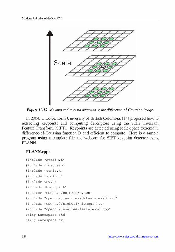
Modern Robotics with OpenCV
180 http://www.sciencepublishinggroup.com
Figure 10.10 Maxima and minima detection in the difference-of-Gaussian image.
In 2004, D.Lowe, form University of British Columbia, [14] proposed how to
extracting keypoints and computing descriptors using the Scale Invariant
Feature Transform (SIFT). Keypoints are detected using scale-space extrema in
difference-of-Gaussian function D and efficient to compute. Here is a sample
program using a template file and webcam for SIFT keypoint detector using
FLANN.
FLANN.cpp:
#include "stdafx.h"
#include <iostream>
#include <conio.h>
#include <stdio.h>
#include <cv.h>
#include <highgui.h>
#include "opencv2/core/core.hpp"
#include "opencv2/features2d/features2d.hpp"
#include "opencv2/highgui/highgui.hpp"
#include "opencv2/nonfree/features2d.hpp"
using namespace std;
using namespace cv;

Chapter 10 Intelligent Humanoid Robot
http://www.sciencepublishinggroup.com 181
int main()
{
int i=0;
CvRect in_box,output_box;
Mat train=imread("template3.jpg"), train_g;
cvtColor(train,train_g,CV_BGR2GRAY);
//detect SIFT keypoints
vector<KeyPoint> train_kp;
Mat train_desc;
SiftFeatureDetector featureDetector;
featureDetector.detect(train_g,train_kp);
SiftDescriptorExtractor featureExtractor;
featureExtractor.compute(train_g, train_kp, train_desc);
//FLANN based descriptor matcher object
FlannBasedMatcher matcher;
vector<Mat> train_desc_collection (1,train_desc);
matcher.add(train_desc_collection);
matcher.train();
//VideoCapture object
VideoCapture cap(0);
unsigned int frame_count=0;
while (char(waitKey(1)) !='q') {
double to=getTickCount();
Mat test, test_g;
cap>>test;
if (test.empty())
continue;
cvtColor(test,test_g,CV_BGR2GRAY);
//detect SIFT keypoint and extract descriptors in the
test image
vector<KeyPoint> test_kp;
Mat test_desc;
featureDetector.detect(test_g, test_kp);
featureExtractor.compute(test_g,test_kp,test_desc);
//match train and test descriptors, getting 2 nearest
neighbors for all test descriptors
vector<vector<DMatch> > matches;

Modern Robotics with OpenCV
182 http://www.sciencepublishinggroup.com
matcher.knnMatch(test_desc,matches,10);
//filter for good matches according to Lowe's algorithm
vector<DMatch> good_matches;
Mat img_show;
vector<KeyPoint> keypoints_1;
vector<KeyPoint> keypoints_2;
for ( i=0;i<matches.size();i++) {
if (matches[i][0].distance <
0.5*matches[i][1].distance)
{
good_matches.push_back(matches[i][0]);
}
}
//-- Localize the object
std::vector<Point2f> obj;
std::vector<Point2f> scene;
drawMatches(test,test_kp, train, train_kp, good_matches,
img_show,Scalar::all(-1), Scalar::all(-
1),vector<char>(),DrawMatchesFlags::NOT_DRAW_SINGLE_POINTS);
Point2f point1;
int average_X=0;int average_Y=0;
if (good_matches.size() >= 4){
for( int i = 0; i < good_matches.size(); i++ )
{
//-- Get the keypoints from the good matches
obj.push_back( train_kp[ good_matches[i].trainIdx ].pt );
scene.push_back(test_kp[ good_matches[i].queryIdx ].pt );
point1=test_kp[ good_matches[i].queryIdx ].pt;
average_X+=point1.x; //get the coordinate of x
}
average_X=(average_X)/good_matches.size();
printf("pointx: %d pointy: %d \n",point1.x, point1.y);
cv::rectangle(img_show , cvPoint( average_X-55, point1.y-50) ,
cvPoint( average_X+50, point1.y+50) , Scalar( 255, 0, 255),
1 );
}
imshow("Matches", img_show);

Chapter 10 Intelligent Humanoid Robot
http://www.sciencepublishinggroup.com 183
cout<<"Frame rate="<<getTickFrequency()/(getTickCount()-
t0)<<endl;
}
return 0;
}
Figure 10.11 Robust Object detector using FLANN based matcher, rectangle line used
to get center position of the object.
References
[1] Adrian Kaehler & Garry Bradksy, Learning OpenCV: Computer Vision in C++
with the OpenCV Library, O'Reilly PUblisher, 2014.
[2] Samarth Brahmbatt, Practical OpenCV, Technology in Action Publisher, 2013.
[3] Daniel bagio et al., Mastering OpenCV with Practical Computer Vision Project,
Packt Publisher, 2012.


Chapter 11
Vision-Based Obstacles Avoidance


http://www.sciencepublishinggroup.com 187
On successful completion of this course, students will be able to:
Describe the problem of obstacle avoidance in service robot.
Develop a program for obstacle avoidance using probabilistic
robotics.
Introduction
In recent years, service robots developed for various applications such as the
personal, medical and welfare robots. Technologies and methods used for
service robots increased drastically to make it more intelligent, and resulting
these kind of robots available commercially.Among the indoor service robots,
those that are able to operate in environments with humans, and especially
those that are able to interact with the customer have gained high interest in
recent years. The major task routinely performed by a service robot (for
example deliver a cup, picking a cup and human robot interaction) are based on
visually perceived information. In order a service robot perform such tasks,
they must also have the ability to perceive and act upon visual information.
Computer Vision is a an important tools for robotics systems since it mimics the
human sense of vision and allows for non-contact measurement of the
environment. A good program using vision sensor will make a service robot
have the ability to detects and identifies detailed object around it (such as face
recognition, distance measurement of obstacle, and free area for path planning).
The main concern when develop a service robot is obstacle avoidance system
and the implementation of stereo camera as an important vision sensor.
Obstacle Avoidance of Service Robot
The development of an obstacle avoidance system for robots to accurately
detect moving obstacles in indoors is challenging task. The navigation and
obstacle avoidance strategy are the important aspects in a vision-based service
robot. Bayesian techniques provide a powerful statistical tool to help manage
measurement uncertainty and perform multisensor fusion and identity
estimation. The advantages of probabilistic robotics are able to accommodate
imperfect sensors (such as camera with noises), robust in real world applications
and best known approach to many hard robotics problem. Based on literatures
obtained by the authors, many research in development of service robot such as

Modern Robotics with OpenCV
188 http://www.sciencepublishinggroup.com
[1][2], whereas task of the service robot is the setting and clearing of tables in a
controlled environment without stereo camera. However, there is no multiple
moving obstacles avoidance method for service robot in indoor environment
exposed especially using stereo camera. The contribution of this chapter is the
introduction of a new method of multiple moving obstacles avoidance for
service robots using a stereo camera in indoor environment.
A mobile robot involving two actuator wheels is considered as a system
subject to nonholonomic constraints and usually using fuzzy logic to control the
motor [5]. Consider an autonomous wheeled mobile robot and position in the
Cartesian frame of coordinates shown in Figure 11.1, where and are the
two coordinates of the origin P of the moving frame and is the robot
orientation angle with respect to the positive x-axis. The rotation angle of the
right and left wheel denoted as and and radius of the wheel by R thus the
configuration of the mobile robot qR can be described by five generalized
coordinates such as:
T
lrRRRR yxq ),,,,( (11.1)
Based on Figure 11.1, is the linear velocity, is the angular velocity,
and are radial and angular coordinate of the robot [6]. The kinematics
equations of motion for the robot given by:
RRR vx cos (11.2)
RRR vy sin (11.3)
RR (11.4)
The angular velocity of the right and left wheel can be obtained by:
dt
d rr
and
dt
d ll
(11.5)
Finally, the linear velocity can be formulated as:
2/)( lrR Rv (11.6)

Chapter 11 Vision-Based Obstacles Avoidance
http://www.sciencepublishinggroup.com 189
Figure 11.1 Cartesian representation of mobile robot.
Based on the model in Figure 11.1, we propose the model of a mobile robot
using a stereo camera with a moving obstacle as shown in Figure 11.2. A
camera as a vision sensor has limitations in view angle to capture an object, so
we define Cam as a maximum angle that moving obstacles can be detected by a
camera used in this research. The location of an object shall consist of the object
position and orientation.

Modern Robotics with OpenCV
190 http://www.sciencepublishinggroup.com
Figure 11.2 General cartesian model of mobile robot using stereo camera.
We have developed a vision-based service robot called Beebot to deliver a
cup to customer with voice recognition and telepresence capabilities using
Tigal EasyVR Shield for Arduino 2.0. The voice recognition system has the
ability for users to create up to 28 of their own custom Speaker Independent (SI)
Command Vocabularies using the Quick T2SI Lite Software (license available
separately). Additionally the EeasyVR 2.0 includes SonicNet technology for
wireless communication between modules or any other sound source. DTMF
tone generation is also included.
Stereo Imaging Model
We have developed a system for face detection using Haar cascade classifier
and depth estimation for measuring distance of peoples as moving obstacles
using stereo vision. In the stereo imaging model, the tree-dimensional points in
stereo camera frame are projected in the left and the right image frame. On the
contrary, using the projection of the points onto the left and right image frame,
the three-dimensional points positions in stereo camera frame can be located.
Figure 11.4 shows the stereo imaging model using the left front image frame LF
and right front image frame RF [9].

Chapter 11 Vision-Based Obstacles Avoidance
http://www.sciencepublishinggroup.com 191
Figure 11.3 Stereo Imaging model.
By using stereo vision, we can obtain the position of each moving obstacle in
the images, then we can calculate and estimate the distance of the moving
obstacle. Kalman filtering used for the stability of the distance estimation. The
three-dimensional point in stereo camera frame can be reconstructed using the
two-dimensional projection of point in left front image frame and in right front
image frame using formula :
SC RI LI1x x x2
SC SC RIy yRI LI
x xSCz
q a ( q q )2
q a qq q
f aq
q (7)
Note that y
RI
y
LI qq
To estimate the direction θdirection of moving obstacle using stereo vision, we
calculate using the figure and formula below:

Modern Robotics with OpenCV
192 http://www.sciencepublishinggroup.com
Figure 11.4 Direction estimation using stereo vision.
θdirection =arc tan
(8)
Probabilistic Robotics for Multiple Obstacle Avoidance
Method
Camera as vision sensor sometimes have distortion, so Bayesian decision
theory used to state estimation and determine the optimal response for the robot
based on inaccurate sensor data. Bayesian decision rule probabilistically
estimate a dynamic system state from noisy observations. Examples of
measurement data include camera images and range scan. If x is a quantity that
we would like to infer from y, the probability p(x) will be referred to as prior
probability distribution. The Bayesian update formula is applied to determine
the new posterior p(x, y) whenever a new observation is obtained:
(11.9)
To apply Bayesian approach for obstacle avoidance where someone who
walks with a direction indicated as an unexpected obstacle, we consider this
obstacle to be a random event. The probabilistic information in z about is
described by a conditional probability density function )|( zp of the
observation vector z. Let denote the state of the path to be a random variable
consisting of four states:

Chapter 11 Vision-Based Obstacles Avoidance
http://www.sciencepublishinggroup.com 193
1 2 3 4( , , , )
(obstacle,no _ obstacle,direction _ right,direction _ left)
(11.10)
If we want a service robot should stay on the path to goal in any case,
strategies to avoid moving obstacle include:
Maneuver to the right, if detected moving obstacle is moving toward the
left. Maneuver to the left, if detected moving obstacle is moving toward
the right.
Stop, if moving obstacle too close to robot detected both by vision and
ultrasonic sensors.
Then, we restrict the action space denoted as A as:
1, 2 3(a a ,a )
maneuver to right, maneuver to left,stop
(11.11)
We define a loss function L(a, θ) which gives a measure of the loss incurred
in taking action a when the state is θ. The robot should chooses an action a
from the set A of possible actions based on the observation z of the current state
of the path θ. This gives the posterior distribution of θ as:
)()|(
)()|()|(
pzp
pzpzp (11.12)
Then, based on the posterior distribution in (11.12), we can compute the
posterior expected loss of an action [14]:
)|(),()),|(( zpaLazpB (11.13)
Multiple Moving Obstacles Avoidance Method and
Algorithm
We have proposed a method and algorithm of obstacles avoidance for service
robot that run from start to goal position, giving a cup to customer and going
back to home. This method will identify a customer, checking moving obstacles
and its distance and take action for maneuver to avoid the collision. Stereo

Modern Robotics with OpenCV
194 http://www.sciencepublishinggroup.com
camera used has limitation such as angle view, this camera only able to capture
object infront of it about 30°. So, when the robot starts to maneuver, the moving
obstacle could be out of view area of camera. So for this experiment, we have
proposes a predefined motion for maneuver based on the estimation speed and
direction of moving obstacle.
Table 11.1 Actions to avoid moving obstacle.
No Speed of moving obstacle Direction of moving obstacle Action
1 Low Approach to robot Manuver slow
2 High Approach to robot Maneuver fast
3 Low Infront of robot Manuver slow
4 High Infront of robot Manuver slow
Figure below shows the proposed model of maneuvering on the service robot,
pL which is the probability of moving obstacle leads to the left, and pR the
probability of moving obstacle leads to the right. By estimating the direction of
motion of the obstacle, then the most appropriate action to avoid to the right /
left side can be determined, to minimize collision with these obstacles. If there
are more than 1 moving obstacle, then robot should identified the nearest
moving obstacle to avoid collision, and the direction of maneuver should be
opposite with the direction of moving obstacle (Figure 7).
Figure 11.5 A maneuvering model to avoids multiple moving obstacle using stereo
vision, 2 multiple moving obstacle with the different direction (a) and the same
direction (b).

Chapter 11 Vision-Based Obstacles Avoidance
http://www.sciencepublishinggroup.com 195
The flowchart of a Navigation system and multiple moving obstacles
avoidance method for vision-based service robot using stereo camera shown in
Figure 11.8. Based on the Figure 8, image captured by stereo camera used as
testing images to be processed by Haar classifier to detect how many people in
the images, and face recognition by PCA. We implement visual tracking for
heading a robot to a customer. Robot continuously measures the distance of
obstacle and send the data to Laptop. The next step is multiple moving obstacle
detection and tracking. If there is no moving obstacle, robot run from start to
goal position in normal speed. The advantage using stereo vision in our system
is the ability to estimate the distance of customer/obstacles (depth estimation)
and direction’s movement of obstacles.
If moving obstacle appeared and collision will occurred, robot will maneuver
to avoids obstacle. The proposed algorithms for obstacles avoidance shown
below:
Algorithm 11.1. Multiple moving obstacles avoidance and maneuvering for
service robot.
Checking a cup sensor // check if cup is loaded or no
Capture face’s images
Face detection and recognition using PCA
if cup loaded and face recognized
// Visual tracking using stereo vision
While (customer !=center screen)
begin
Heading robot to customer’s position
end
if (position of customer at center screen)
begin
Go to customer
call movingObstaclesIdentification
Bayesian processing
if moving obstacle==true and min_distance=true and
goal=false
maneuvering the robot
end if
Giving a glass
Go to home

Modern Robotics with OpenCV
196 http://www.sciencepublishinggroup.com
end
end if
end
// Function to detects and tracks a moving obstacle
function movingObstacleIdentification
moving obstacle detection // Using Haar cascade
classifier
if (moving_obstacle==true) then
//estimate distance between robot and moving obstacle
using stereo vision
distance estimation // Using Stereo camera and Kalman
filtering
// estimate velocity and direction of moving obstacle
Calculate Ov , direction
Endif
Return Ov , direction
end function

Chapter 11 Vision-Based Obstacles Avoidance
http://www.sciencepublishinggroup.com 197
Figure 11.6 Flowchart of A Navigation system and Multiple moving obstacles
avoidance method for vision-based service robot using stereo camera.
The result of improved face recognition system using PCA shown in Figure
11.7, where 1 customer succesfully identified with his order. Before delivering a
cup, visual tracking applied to directs a robot to an identified customer. Robot
succesfully go to the identified customer using our proposed method.

Modern Robotics with OpenCV
198 http://www.sciencepublishinggroup.com
Figure 11.7 An example of face detected and recognized together with his order using
our framework of face recognition system.
Multiple Moving Obstacle Avoidance Using Stereo Vision
The result of identifying multiple moving obstacle shown in figure below, the
advantages if we using stereo vision, we can estimate the distance and
direction/angle of the moving obstacle. The value probability of obstacle/no
obstacle also run well for make a robotics system more robust as as shown
Figure 11.8.

Chapter 11 Vision-Based Obstacles Avoidance
http://www.sciencepublishinggroup.com 199
(a)
(b)
Figure 11.8 value probability of obstacle/no obstacle, (a). results of distance and
direction estimation, (b). implementation of probabilistics robotics for moving obstacles
avoidance using stereo images.

Modern Robotics with OpenCV
200 http://www.sciencepublishinggroup.com
Figure 11.9 Result of moving obstacle avoidance using stereo vision and Bayesian
approach. Sequence action of service robot shown from (a) until (f) to deliver a cup to
an identified customer and go back to home.
For experiment delivering a cup to a customer, the setup experiment is in
indoor where a customer and not customer sat on the chair, and there is

Chapter 11 Vision-Based Obstacles Avoidance
http://www.sciencepublishinggroup.com 201
someone that walking as a moving obstacle as shown below. Robot successfully
identifies a moving obstacle, avoid the collision, giving a cup to a customer then
go back to home. For 10 (ten) times experiment using Bayesian approach, the
success rate to identify moving obstacle is 90%, and without Bayesian approach
is 60%. The very interesting video to show the action of this robot can be
viewed at: http://www.youtube.com/watch?v=n181CtvGJ88.
References
[1] Acosta, L., González, E.J., Rodríguez, J.N., Hamilton, A.F., Méndez J.A.,
Hernéndez S., Sigut S.M, and Marichal G.N. Design and Implementation of a
Service Robot for A Restaurant. International Journal of robotics and automation.
2006; vol. 21(4): pp. 273-281.
[2] Qing-wiau Y., Can Y., Zhuang F. and Yan-Zheng Z. Research of the Localization
of Restaurant Service Robot. International Journal of Advanced Robotic Systems.
2010; vol. 7(3): pp. 227-238.
[3] Chatib, O., Real-Time Obstacle Avoidance for Manipulators and Mobile Robots.,
The International Journal of Robotics Research, 1986; vol. 5(1), pp. 90-98.
[4] Borenstein, J., Koren, Y., The Vector Field Histogram- Fast Obstacle Avoidance
for Mobile Robots, in proc. IEEE Trans. On Robotics and Automation. 1991; vol
7(3): pp.278-288.
[5] S. Nuryono, Penerapan Multi Mikrokontroler pada Model Robot Mobil
Menggunakan Logika Fuzzy, Journal Telkomnika, 2009, vol. 7(3), pp, 213-218.
[6] Masehian E., Katebi Y. Robot Motion Planning in Dynamic Environments with
Moving Obstacles and Target. International Journal of Mechanical Systems
Science and Engineering. 2007; vol. 1(1), pp. 20-29.
[7] Budiharto, W., Purwanto, D. and Jazidie, A. A Robust Obstacle Avoidance for
Service Robot using Bayesian Approach. International Journal of Advanced
Robotic Systems. Intech Publisher – Austria. 2011; Vol. 8(1): pp. 52-60.
[8] Budiharto, W., Purwanto, D. & Jazidie, A. A Novel Method for Static and Moving
Obstacle Avoidance for Service robot using Bayesian Filtering. Proceeding of
IEEE 2nd International conf. on Advances in Computing, Control and
Telecommunications Technology.2010; pp. 156-160. DOI: 10.1109/ACT.2010.51.
[9] Purwanto, D. Visual Feedback Control in Multi-Degrees-of-Freedom Motion
System. PhD thesis at Graduate School of Science and Technology - Keio
University, Japan. 2001.

Modern Robotics with OpenCV
202 http://www.sciencepublishinggroup.com
[10] Turk, M. & Pentland A. Eigenfaces for recognition. International Journal of
Cognitive Neuroscience. 1991; vol. 3(1): pp. 71-86.
[11] Belhumeur, P. & Kriegman, D. What is the set of images of an object under all
possible illumination conditions. International Journal of Computer Vision. 1998;
Vol. 28( 3), pp. 245-260.
[12] Etemad, K. & Chellappa R . Discriminant analysis for recognition of human face
images. Journal of the Optical Society of America A. 1997; vol. 14( 8): pp. 1724-
1733.
[13] Budiharto, W., Santoso A., Purwanto, D. and Jazidie, A. An Improved Face
recognition System for Service Robot using Stereo Vision. In: Tudor Barbu Editor.
Face Recognition / Book 3. Intech Publisher – Austria; 2011: pp. 1-12.
[14] Hu, H. & Brady, M. A Bayesian Approach to Real-Time Obstacle Avoidance for a
Mobile Robot. Autonomous Robots. 1994; vol. 1: pp. 69-92.
Chapter 12
Vision-Based Manipulator


http://www.sciencepublishinggroup.com 205
On successful completion of this course, students will be able to:
Explain how the manipulator works.
Describe types of manipulator.
Develop a vision-based manipulator.
Introduction
One of the most common of manipulation tasks is grasping an object. Tasks
performed by humans involve some form of grasping action. In the absence of
feedback, the grasping action cannot be completed effectively. A human being
grasps an object almost invariably with the aid of vision. We use visual
information to identify and locate the object, and then decide how to grasp them.
Inverse Kinematics
In a two-joint arm robot, given the angles of the joints, the kinematics
equations give the location of the tip of the arm. Inverse kinematics refers to the
reverse process. Given a desired location for the tip of the robotic arm, what
should the angles of the joints be so as to locate the tip of the arm at the desired
location? There is usually more than one solution and can at times be a difficult
problem to solve. In a 2-dimensional input space, with a two-joint robotic arm
and given the desired co-ordinate, the problem reduces to finding the two angles
involved. The first angle is between the first arm and the ground (or whatever it
is attached to). The second angle is between the first arm and the second arm.
Figure 12.1 inverse kinematics for 2 DOF arm robot[12].

Modern Robotics with OpenCV
206 http://www.sciencepublishinggroup.com
For simple structures like the two-joint robotic arm, it is possible to
mathematically deduce the angles at the joints given the desired location of the
tip of the arm. However with more complex structures (eg: n-joint robotic arms
operating in a 3-dimensional input space) deducing a mathematical solution for
the inverse kinematics may prove challenging. Using fuzzy logic, we can
construct a Fuzzy Inference System that deduces the inverse kinematics if the
forward kinematics of the problem is known, hence sidestepping the need to
develop an analytical solution.
Vision-Based Manipulator
Most work in robotic manipulation assumes a known 3-D model of the object
and the environment, and focuses on designing control and planning methods to
achieve a successful and stable grasp in simulation environments. Grasping is
usually preceded by a number of tasks that effect the final grasping action. The
sequence of steps involved is:
1) The movement of the end-effector from a given position to within a
reaching position from the object.
2) The estimation of grasp points and orientation of the end-effector to
perform the grasp operation.
3) The grasping action, once the end effector is in the appropriate position.
Based on the previous literature (visual-servoing) is huge and largely
unorganized. A variety of methods have been proposed to solve vision-based
manipulation [1-5]. They use vision to aid just one of the above mentioned steps.
In the past, most approaches to robotic grasping [6] [7] assume availability of a
complete 3-D model of the object to be grasped. In practice, however, such a
model is often not available—the 3D models obtained from a stereo system are
often noisy with many points missing, and 3-D models obtained from a laser
system are very sparse. This makes grasping a hard problem in practice. In
more general grasping, Kamon et al. [8] used Q-learning to control the arm to
reach towards a spherical object to grasp it using a parallel plate gripper.
For grasping 2D planar objects, most prior work focuses on finding the
location of the fingers given the object contour, which one can find quite
reliably for uniformly colored planar objects lying on a uniformly colored table
top. Using local visual features (based on the 2-d contour) and other properties
such as force and form closure, the methods discussed below decide the 2D
location at which to place the fingertips (two or three) to grasp the object.

Chapter 12 Vision-Based Manipulator
http://www.sciencepublishinggroup.com 207
Edsinger and Kemp [9] grasped cylindrical objects using a power grasp by
using visual servoing and do not apply to grasping for general shapes. An
inverse kinematic solver is proposed in [10] to find all joint angles for given
position of the effectors on the manipulator. The target object is recognized by
color segmentation. The 3D position is computed by the stereo vision system
after contour extraction.
Inverse kinematics of manipulator and object location are the key technology
for arm robot. We study various visual feedback methods from previous
literature and develop a new model for grasping a bottle. We know that
Extraction of image information and control of a robot are two separate tasks
where at first image processing is performed followed by the generation of a
control sequence. A typical example is to recognize the object to be
manipulated by matching image features to a model of the object and compute
its pose relative to the camera (robot) coordinate system. In general method,
first the target object is recognized by the vision system which than estimates
the 3D pose of the object. Based on this information, the controller coordinates
to move the arm robot to grasp the object/bottle. The framework proposed in
this experiment shown in fig. 12.2 below, where the stereo camera for pose
estimation attached about 50cm at the side of manipulator.
Figure 12.2 example of vision-based grasping using stereo vision.

Modern Robotics with OpenCV
208 http://www.sciencepublishinggroup.com
We developed a framework of vision-based arm robot using 4 DOF (Degree
of Freedom) arm robot from Lynxmotion that able to delivers fast, accurate, and
repeatable movement. The robot features: base rotation, single plane shoulder,
elbow, wrist motion, a functional gripper, and optional wrist rotate as shown in
figure 12.3. This robotic arm is an affordable system with a time tested rock
solid design that will last and last.
Figure 12.3 4 DOF arm robot using stereo vision used in the experiment.
The specification of this manipulator:
Base: Height = 6.9 cm
Hand/Grip: Max Length (No Wrist Rotate) = 8.7 cm
Hand/Grip: Max Length (With LW Rotate) = 11.3 cm
Hand/Grip: Max Length (With HD Rotate) = 10.0 cm
Length: Forearm = 12.7 cm
Length: Arm = 11.9 cm
Grasping Model
Grasp determination is probably one of the most important questions from
manipulation point of view. Usually, the object is of unknown shape. In our
model, we propose a simple way, if we know the distance of the bottle then
move the arm to that position, then when the center point of a bottle exactly
meet the center point of the gripper, then it means that is the time for grasping
the bottle/object as shown in figure 12.4:

Chapter 12 Vision-Based Manipulator
http://www.sciencepublishinggroup.com 209
Figure 12.4 Finding the center of the bottle using vision (a) and color marking for
indicating the position of gripper with an object [11].
The proposed algorithm for detect an object/bottle, grasp it and move to the
destination is shown below:
do
detect the object/bottle
if object/bottle detected then
begin
find position of the object/bottle
move arm robot to the object/bottle
move the gripper to the center of the object/bottle
if the position equal
grasp the object/bottle
else
move to gripper to the center of the object/bottle
end
endif
move the object to destination
go to the initial position
loop
An environment consists of a variety of objects, such as the robot itself, walls,
floor, tables, objects to be grasped, etc. In order to successfully move the arm

Modern Robotics with OpenCV
210 http://www.sciencepublishinggroup.com
without hitting an obstacle, we provide 1 distance sensor at the gripper. To
determine the state of the object, the "good" grasp position should be first
determined. The experiment conducted at our lab to grasp and move a bottle to
the destination. For testing the connection of hardware, we use Lynx SSC-32 as
shown below:
Figure 12.5 using Lynx SSC-32 Terminal for testing the hardware [13].
We use Lynxmotion RIOS (Robotic Arm Interactive Operating System) SSC-
32 software to configure and control the arm robot as shown in figure 12.6:

Chapter 12 Vision-Based Manipulator
http://www.sciencepublishinggroup.com 211
Figure 12.6 Configuring and control the board of arm robot using RIOS SSC-32
Software[13].
After configuring and calibrating the servos of arm robot. We put an
object/bottle in front of the arm robot to be grasped and move to other position.
Based on our experiment we get the expected result as shown in table 12.1.
Table 12.1 Result of Detecting and Grasping an Object in 10x.
No Action Success failure
1 Identify the object as bottle 100% 0%
2 Grasping an object correctly 90% 10%
3 Estimate the distance of the bottle 90% 10%
The accuracy and robustness of the system and the algorithm were tested and
proven to be effective in real scenarios.
Program for object detection and grasping successfully developed with
OpenCV and the manipulator able to grasp it as shown in figure 12.7

Modern Robotics with OpenCV
212 http://www.sciencepublishinggroup.com
Figure 12.7 Object detection and grasping OpenCV.
Exercise
1) Create a simulator program for inverse kinematics using function as shown
below:
data = Convert.ToInt32(txtInput.Text);
MessageBox.Show("value from sin " + data + " "
+Convert.ToString(Math.Sin(Radians2Degrees(data))));
MessageBox.Show("value from cos " +data + " "
+Convert.ToString(Math.Cos(Radians2Degrees(data))));
MessageBox.Show("value from tan " + data + " "+
Convert.ToString(Math.Tan(Radians2Degrees(data))));
MessageBox.Show("value from Theta(Asin) : " +
Convert.ToString((Math.Asin(Math.Sin(Radians2Degrees(data))))*(18
0/Math.PI)));
MessageBox.Show("value from Theta(Acos) : " +
Convert.ToString((Math.Acos(0.866))*(180/Math.PI) ));

Chapter 12 Vision-Based Manipulator
http://www.sciencepublishinggroup.com 213
MessageBox.Show("value from Theta(Atan) : " +
Convert.ToString((Math.Atan(Math.Tan(Radians2Degrees(data)))) *
(180 / Math.PI)));
MessageBox.Show("value from Theta2(arccos) : " +
Convert.ToString((Math.Acos(Math.Cos(Radians2Degrees( (((x*x)+(y*
y))-(l1*l1)-(l2*l2))/(2*l1*l2) )))) * (180 / Math.PI)));
Figure 12.7 Inverse Kinematics Simulator.
2) Create a program to grasp an object using arm robot and stereo vision.
References
[1] A. Bendiksen and G. D. Hager. “A vision-based grasping system for unfamiliar
planar objects“. In ICRA, pages2844–2849, 1994.
[2] H. I. Christensen and P. L. Corke. “Visual servoing“. I. J.Robotic Res., 22(10-
11):779–780,2003.
[3] D. Kragic and H. I. Christensen. “A framework for visual servoing“. In ICVS,
pages 345–354, 2003
[4] A. Bicchi and V. Kumar, “Robotic grasping and contact: a review,” in ICRA, 2000.

Modern Robotics with OpenCV
214 http://www.sciencepublishinggroup.com
[5] J. Jiao, Embedded Vision-Based Autonomous Move-to-Grasp Approach for a
Mobile Manipulator,International Journal of Advanced Robotics System, vol. 9,
pp.1-6, 2012.
[6] K. Shimoga, “Robot grasp synthesis: a survey,” IJRR, vol. 15, pp. 230–266, 1996.
[7] D. Purwanto. Visual Feedback Control in Multi-Degrees-of-Freedom Motion
System. PhD thesis at Graduate School of Science and Technology - Keio
University, Japan, 2001.
[8] I., Kamon, T. Flash, and S. Edelman, “Learning to grasp using visual information,”
in ICRA, 1996.
[9] A. Edsinger and C. C. Kemp, “Manipulation in human environments,” in
IEEE/RAS Int’l Conf on Humanoid Robotics (Humanoids06), 2006.
[10] Y. Yang, “Binocular Stereo Vision based Humanoid Manipulator Control”, 30th
International Conference on Control, pp. 3996 - 4001, China. 2011.
[11] Widodo Budiharto, Bayu Kanigoro and Anita Rahayu, Vision-Based Grasping for
Manipulator using Object Features, Annual Conference on Engineering and
Information Technology, pp. 228-235, Japan, March 28-30th, 2014.
[12] Matworks.com.
[13] www.lynxmotion.com.

http://www.sciencepublishinggroup.com 215
Glossary
Artificial Intelligence: is the mimicking of human thought and cognitive
processes to solve complex problems automatically. AI uses techniques for
writing computer code to represent and manipulate knowledge.
Autonomous: Operating without pre-programmed behaviors and without
supervision from humans.
Action-Based Planning: The goal of action-based planning is to determine
how to decompose a high level action into a network of sub actions that perform
the requisite task. Therefore the major task within such a planning system is to
manage the constraints that apply to the interrelationships (e.g., ordering
constraints) between actions. In fact, action-based planning is best viewed as a
constraint satisfaction problem.
Agents: Agents are software programs that are capable of autonomous, flexible,
purposeful and reasoning action in pursuit of one or more goals. They are
designed to take timely action in response to external stimuli from their
environment on behalf of a human. When multiple agents are being used
together in a system, individual agents are expected to interact together as
appropriate to achieve the goals of the overall system.
Agent Architecture: There are two levels of agent architecture, when a number
of agents are to work together for a common goal. There is the architecture of
the system of agents, that will determine how they work together, and which
does not need to be concerned with how individual agents fulfill their sub-
missions; and the architecture of each individual agent, which does determine
its inner workings.
Algorithm: An algorithm is a set of instructions that explain how to solve a
problem. It is usually first stated in English and arithmetic, and from this, a
programmer can translate it into executable code (that is, code to be run on a
computer).

Modern Robotics with OpenCV
216 http://www.sciencepublishinggroup.com
Associative Memories: Associative memories work by recalling information in
response to an information cue. Associative memories can be auto associative or
hetero associative. Auto associative memories recall the same information that
is used as a cue, which can be useful to complete a partial pattern.
Camera: A camera is a device used to take pictures, either singly or in
sequence. A camera that takes pictures singly is sometimes called a photo
camera to distinguish it from a video camera.
Decision Theory: Decision theory provides a basis for making choices in the
face of uncertainty, based on the assignment of probabilities and payoffs to all
possible outcomes of each decision. The space of possible actions and states of
the world is represented by a decision tree.
Degrees of Freedom: The number of independent variables in the system. Each
joint in a serial robot represents a degree of freedom.
Dexterity: A measure of the robot's ability to follow complex paths.
Dynamic Model: A mathematical model describing the motions of the robot
and the forces that cause them.
Egomotion: determining the 3D rigid motion (rotation and translation) of the
camera from an image sequence produced by the camera.
Tracking: following the movements of a (usually) smaller set of interest points
or objects (e.g., vehicles or humans) in the image sequence.
Optical Flow: to determine, for each point in the image, how that point is
moving relative to the image plane, i.e., its apparent motion. This motion is a
result both of how the corresponding 3D point is moving in the scene and how
the camera is moving relative to the scene.
End-Effector: The robot's last link. The robot uses the end-effector to
accomplish a task. The end-effector may be holding a tool, or the end-effector
itself may be a tool. The end-effector is loosely comparable to a human's hand.

Chapter 12 Vision-Based Manipulator
http://www.sciencepublishinggroup.com 217
Edge Detection: Edge Detection marks the points in a digital image at which
the luminous intensity changes sharply.
Expert System: An expert system encapsulates the specialist knowledge gained
from a human expert (such as a bond trader or a loan underwriter) and applies
that knowledge automatically to make decisions.
Frame grabber: An electronic device that captures individual, digital still
frames from an analog video signal or a digital video stream.
Game Theory: Game theory is a branch of mathematics that seeks to model
decision making in conflict situations.
Grayscale: A grayscale digital image is an image in which the value of each
pixel is a single sample. Displayed images of this sort are typically composed of
shades of gray, varying from black at the weakest intensity to white at the
strongest, though in principle the samples could be displayed as shades of any
color, or even coded with various colors for different intensities.
Genetic Algorithms: Search algorithms used in machine learning which
involve iteratively generating new candidate solutions by combining two high
scoring earlier (or parent) solutions in a search for a better solution.
HSV Color Space: The HSV (Hue, Saturation, Value) model, also called HSB
(Hue, Saturation, Brightness), defines a color space in terms of three constituent
components: Hue, the color type (such as red, blue, or yellow), Saturation, the
"vibrancy" of the color and colorimetric purity and Value, the brightness of the
color.
Inference Engine: The part of an expert system responsible for drawing new
conclusions from the current data and rules. The inference engine is a portion of
the reusable part of an expert system (along with the user interface, a knowledge
base editor, and an explanation system), that will work with different sets of
case-specific data and knowledge bases.

Modern Robotics with OpenCV
218 http://www.sciencepublishinggroup.com
Inverse Kinematics: The inverse kinematics problem is to find the robot's joint
displacements given position and orientation constraints on the robot's end-
effector.
Jacobian: The matrix of first-order partial derivatives. For robots, the Jacobian
relates the end- effector velocity the joint speeds.
Joint Space: A coordinate system used to describe the state of the robot in
terms of its joint states. Inverse kinematics may also be thought of as a mapping
from end-effector space to joint space.
Machine Learning: refers to the ability of computers to automatically acquire
new knowledge, learning from, for example, past cases or experience, from the
computer's own experiences, or from exploration.
Machine Vision: Machine Vision is the application of computer vision to
industry and manufacturing.
Motion Perception: MP is the process of inferring the speed and direction of
objects and surfaces that move in a visual scene given some visual input.
Neural Networks: Neural Networks are an approach to machine learning which
developed out of attempts to model the processing that occurs within the
neurons of the brain. By using simple processing units (neurons), organized in a
layered and highly parallel architecture, it is possible to perform arbitrarily
complex calculations. Learning is achieved through repeated minor
modifications to selected neurons, which results in a very powerful
classification system.
Pattern Recognition: This is a field within the area of machine learning.
Alternatively, it can be defined as the act of taking in raw data and taking an
action based on the category of the data. It is a collection of methods for
supervised learning.
Pixel: A pixel is one of the many tiny dots that make up the representation of a
picture in a computer's memory or screen.

Chapter 12 Vision-Based Manipulator
http://www.sciencepublishinggroup.com 219
Pixelation: In computer graphics, pixelation is an effect caused by displaying a
bitmap or a section of a bitmap at such a large size that individual pixels, small
single-colored square display elements that comprise the bitmap, are visible.
Simulated Annealing: Simulated annealing is an optimization method based on
an analogy with the physical process of toughening alloys, such as steel, called
annealing.
Serial Robot: A serial robot is a single chain of joints connected by links.
Singularity: A position in the robot's workspace where one or more joints no
longer represent independent controlling variables. Commonly used to indicate
a position where a particular mathematical formulation fails.
Statics: The study of forces that do not cause motion.
Velocity-Level: Mathematical formulations working with the joint speeds.
Integrating the joint speeds once provides the displacements. See acceleration-
level and position-level.
Workspace: The maximum reach space refers to all of the points the robot can
possibly reach. The dexterous workspace is all of the possible points the robot
can reach with an arbitrary orientation. The dexterous workspace is usually a
subspace of the maximum reach space.