HAL Id: tel-00747213https://tel.archives-ouvertes.fr/tel-00747213

Submitted on 30 Oct 2012

HAL is a multi-disciplinary open accessarchive for the deposit and dissemination of sci-entific research documents, whether they are pub-lished or not. The documents may come fromteaching and research institutions in France orabroad, or from public or private research centers.

L’archive ouverte pluridisciplinaire HAL, estdestinée au dépôt et à la diffusion de documentsscientifiques de niveau recherche, publiés ou non,émanant des établissements d’enseignement et derecherche français ou étrangers, des laboratoirespublics ou privés.

Moderate Reynolds number flow. Application to thehuman upper airways.

Annemie Van Hirtum

To cite this version:Annemie Van Hirtum. Moderate Reynolds number flow. Application to the human upper airways..Fluids mechanics [physics.class-ph]. Université de Grenoble, 2011. <tel-00747213>

Grenoble University, France

Moderate Reynolds number flow. Application to the human upper airways.

HABILITATION A DIRIGER DES RECHERCHES

Presented by

Annemie VAN HIRTUM

CNRS research fellow

30 June 2011

Jury

M. Xavier Pelorson, President

M. Jan-Bert Flor, Reviewer

M. Joel Gilbert, Reviewer

M. Jean-Christophe Valiere, Reviewer

M. Avraham Hirschberg, Examinator

M. Pierre-Yves Lagree, Examinator

Bestijg de trein nooit zonder uw valies met dromen,

dan vindt ge in elke stad behoorlijk onderkomen.

Zit rustig en geduldig naast het open raam:

gij zijt een reiziger en niemand kent uw naam.

Zoek in ’t verleden weer uw frisse kinderogen,

kijk nonchalant en scherp, droomrig en opgetogen.

Al wat ge groeien ziet op ’t zwarte voorjaarsland,

wees overtuigd: het werd alleen voor u geplant.

Laat handelsreizigers over de filmcensuur

hun woordje zeggen: God glimlacht en kiest zijn uur.

Groet minzaam de stationschefs achter hun groen hekken,

want zonder hun signaal zou nooit een trein vertrekken.

En als de trein niet voort wil, zeer ten detrimente

van uwe lust en hoop en zuurbetaalde centen,

Blijf kalm en open uw valies; put uit zijn voorraad

en ge ondervindt dat nooit een enkel uur te loor gaat.

En arriveert de trein in een vreemdsoortig oord,

waarvan ge in uw bestaan de naam nooit hebt gehoord,

Dan is het doel bereikt, dan leert gij eerst wat reizen

betekent voor de dolaards en de ware wijzen...

Wees vooral niet verbaasd dat, langs gewone bomen,

een doodgewone trein u voert naar ’t hart van Rome.

Bericht aan de reizigers,

Jan van Nijlen (1934).

2

Thank you ...

The current document deals with research from 2004-2010 during which my main research activities correspond to

the title of this document: “Moderate Reynolds number flow. Application to the human upper airways.”

Past, current and future results benefit from an important contribution of many persons. Thanks ! Arigato ! Merci !

Dank !

Grenoble, 2011

Annemie

3

Contents

Thank you ... 3

I Scientific summary 6

1 Introduction 7

2 Fluid flow modelling 9

2.1 Viscosity and flow separation . . . . . . . . . . . . . . . . . . . . . . . . . . . . . . . . . . . . . . 9

2.2 One-dimensional flow model with ad-hoc viscosity correction . . . . . . . . . . . . . . . . . . . . 9

2.3 Boundary layer solution . . . . . . . . . . . . . . . . . . . . . . . . . . . . . . . . . . . . . . . . . 10

2.4 Reduced Navier Stokes/Prandtl . . . . . . . . . . . . . . . . . . . . . . . . . . . . . . . . . . . . . 11

2.5 Two-dimensional laminar Navier-Stokes . . . . . . . . . . . . . . . . . . . . . . . . . . . . . . . . 12

2.6 Large Eddy Simulation . . . . . . . . . . . . . . . . . . . . . . . . . . . . . . . . . . . . . . . . . 12

3 Experimental conditions, measurement and nozzles 14

3.1 Range of flow conditions . . . . . . . . . . . . . . . . . . . . . . . . . . . . . . . . . . . . . . . . 14

3.2 Experimental setup and measurement . . . . . . . . . . . . . . . . . . . . . . . . . . . . . . . . . 15

3.2.1 Hot-wire/film calibration . . . . . . . . . . . . . . . . . . . . . . . . . . . . . . . . . . . . 16

3.2.2 Smoke visualisation . . . . . . . . . . . . . . . . . . . . . . . . . . . . . . . . . . . . . . 17

3.2.3 Acoustic insulation box . . . . . . . . . . . . . . . . . . . . . . . . . . . . . . . . . . . . 18

3.3 Nozzles and mechanical replicas . . . . . . . . . . . . . . . . . . . . . . . . . . . . . . . . . . . . 21

3.3.1 Rigid axisymmetrical nozzles . . . . . . . . . . . . . . . . . . . . . . . . . . . . . . . . . 21

3.3.2 Rigid rectangular nozzles . . . . . . . . . . . . . . . . . . . . . . . . . . . . . . . . . . . . 23

3.3.3 Deformable mechanical replicas . . . . . . . . . . . . . . . . . . . . . . . . . . . . . . . . 26

4 Characterisation of jet development 30

4.1 Round free jet development . . . . . . . . . . . . . . . . . . . . . . . . . . . . . . . . . . . . . . . 30

4.1.1 Extended convergent-divergent nozzle . . . . . . . . . . . . . . . . . . . . . . . . . . . . . 31

4.1.2 Extended sharp contraction nozzle . . . . . . . . . . . . . . . . . . . . . . . . . . . . . . . 33

4.1.3 Mean jet decay model parameters . . . . . . . . . . . . . . . . . . . . . . . . . . . . . . . 36

4.2 Rectangular free jet development . . . . . . . . . . . . . . . . . . . . . . . . . . . . . . . . . . . . 37

4.2.1 Rectangular nozzle with 1 sharp obstacle . . . . . . . . . . . . . . . . . . . . . . . . . . . 37

5 Validation of flow models 41

5.1 Convergent axisymmetrical nozzle . . . . . . . . . . . . . . . . . . . . . . . . . . . . . . . . . . . 41

5.2 Asymmetrical constriction . . . . . . . . . . . . . . . . . . . . . . . . . . . . . . . . . . . . . . . 43

5.3 Constriction shapes: fixed and movable . . . . . . . . . . . . . . . . . . . . . . . . . . . . . . . . 44

4

5.4 Rectangular nozzle with 1 gradual and 1 sharp obstacle . . . . . . . . . . . . . . . . . . . . . . . . 46

5.5 Rectangular nozzle with 1 sharp obstacle . . . . . . . . . . . . . . . . . . . . . . . . . . . . . . . . 48

6 Applications to the upper airways 51

6.1 Phonation . . . . . . . . . . . . . . . . . . . . . . . . . . . . . . . . . . . . . . . . . . . . . . . . 51

6.1.1 Theoretical model and stability analysis . . . . . . . . . . . . . . . . . . . . . . . . . . . . 51

6.1.2 Example of results . . . . . . . . . . . . . . . . . . . . . . . . . . . . . . . . . . . . . . . 55

6.2 Voiceless sound production: fricatives . . . . . . . . . . . . . . . . . . . . . . . . . . . . . . . . . 55

6.3 Obstructive sleep apnea . . . . . . . . . . . . . . . . . . . . . . . . . . . . . . . . . . . . . . . . . 57

7 Conclusion and perspectives 59

7.1 Conclusion . . . . . . . . . . . . . . . . . . . . . . . . . . . . . . . . . . . . . . . . . . . . . . . 59

7.1.1 Experiments . . . . . . . . . . . . . . . . . . . . . . . . . . . . . . . . . . . . . . . . . . 59

7.1.2 Characterisation of jet development . . . . . . . . . . . . . . . . . . . . . . . . . . . . . . 60

7.1.3 Validation of flow models . . . . . . . . . . . . . . . . . . . . . . . . . . . . . . . . . . . 60

7.1.4 Application to the upper airways . . . . . . . . . . . . . . . . . . . . . . . . . . . . . . . . 61

7.2 Perspectives . . . . . . . . . . . . . . . . . . . . . . . . . . . . . . . . . . . . . . . . . . . . . . . 61

References 69

II Administrative summary 70

5

Part I

Scientific summary

6

Chapter 1

Introduction

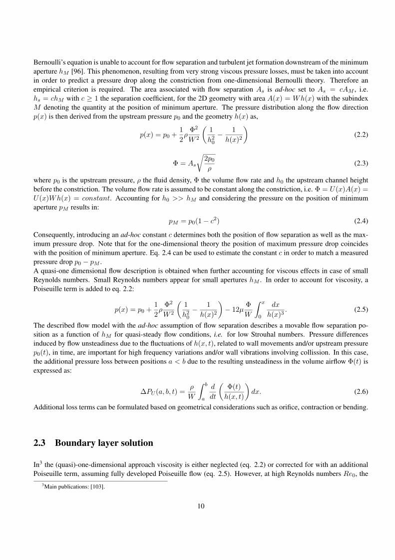
The study of fluid flow is an amasingly ordinary as well as fascinating subject. During the past few years I had

the opportunity to work as a researcher in the field of fluid flow modelling applied to airflow through the human

upper airways and related phenomena such as speech production, . . . The current document is a brief report on the

research to which I participated aiming a small contribution to this rich and stimulating research area.

Airflow through the human upper airways is due to physiological and anatomical properties characterised by veloci-

ties U and geometrical scales h which are, compared to airflows studied in other biofluids fields: small when dealing

with e.g. aeronautics, geophysics or even cosmic flows and large when compared to dimensions and velocities en-

countered e.g. algae or bacterial biofluids. Consequently, typical Reynolds numbers Re ∝ Uh are of the order of

magnitude of 103 which results in moderate Reynolds number flows.

Under certain conditions, quantitatively expressed by additional non-dimensional numbers related to e.g. unsteadi-

ness or compressibility, flows characterised by moderate Reynolds numbers can be described by simplifications of

the governing continuity and Navier-Stokes momentum equations as expressed by: boundary layer equations, self-

similar solutions or an irrotational flow description. Besides the mentioned flow models, a start is made in order to

account for turbulence as well as to formulate simple inverted flow models. It is intriguing to see how (relatively)

complex problems can be simplified and represented within a simple formulation.

Besides flow modelling, qualitative as well as quantitative characterisation and validation of the flow field and re-

lated physical variables is required in order to determine the accuracy and relevance of the applied models and their

dependence on input parameters, initial conditions etc. To this aim, several experimental setups and mechanical

in-vitro replicas are used, improved or developed in order to study the flow field as well as related variables in a

controlled and reproducible way. Although in-vivo observations of upper airway characteristics are the source of

inspiration to build mechanical replicas, their actual design is a combination of additional factors: 1) it is aimed

to reproduce experimentally the relevant range of non-dimensional numbers, 2) to facilitate accurate measurements

with the sensors available in the experimental setup, 3) severe simplifications of the reality in order to study one

particular feature, 4) limitations imposed by manufacturing etc. As a result, mechanical replicas might disappoint

when expecting a duplicate of a portion of real life human upper airways. Nevertheless, simple replicas are more

elegant since they allow to focus on a particular problem.

In addition to experimental validation, data are obtained from numerical simulation of the flow field. An one hand,

7

numerical data provide information of the flow field for which in-vitro data are difficult or impossible to be obtained.

On the other hand, the outcome of numerical simulations can be validated on the experimental measurements.

Applications of airflow through the human upper airways, such as speech production or obstructive sleep apnea,

are partly due to a fluid-structure interaction between airflow coming from the lungs and the upper airways tissues.

Consequently, besides a flow model, a mechanical or/and acoustic model is required as well.

The topics outlined in this introduction are elaborated and illustrated in the following sections1. Finally, conclusions

and perspectives are presented.

Good reading !

1Most relevant publications are mentionned.

8

Chapter 2

Fluid flow modelling

Based on the given orders of magnitude a dimensional analysis is performed. This yields a set of nondimensional

numbers that can be interpreted as a measure of the importance of various flow effects from which several flow

assumptions can be formulated [7, 87, 111].

Following the characteristic aspect ratio (h/W << 1) the flow is assumed to be characterised by a bidimensional

(2D) flow description in the (x, y)-plane with h a typical minimum aperture and W a typical width. In case ve-

locities are small compared with the speed of sound in air, so that the flow is assumed to be incompressible, i.e.

squared Mach number Ma2 << 1. Furthermore, for low Strouhal number (Sr << 1) the airflow is considered

as primarily steady. Finally, as a first approximation, the flow is assumed to be inviscid considering characteristic

Reynolds numbers (Re0 >> 1).

2.1 Viscosity and flow separation

Although1 it can be neglected for the bulk flow considering Reynolds numbersRe0, the occurrence of flow separation

due to viscosity strongly influences the flow development. Therefore, flow separation can not be neglected. In the

studied flow models, the position of flow separation is determined either by an empirical ad-hoc assumption or

predicted based on vanishing wall shear stress, τ(x)=0, along the diverging portion of the wall where the flow is

retarding, with

τ(x) = µ0

(

∂u

∂y

)

y=wall

, (2.1)

and u(x, y) the flow velocity within the boundary layer.

2.2 One-dimensional flow model with ad-hoc viscosity correction

Under2 the assumptions of one-dimensional, laminar, fully inviscid, steady and incompressible flow, one-dimen-

sional Bernoulli’s equation can be used to estimate the pressure and velocity distribution within a constriction.

1Main publications: [103].2Main publications: [19].

9

Bernoulli’s equation is unable to account for flow separation and turbulent jet formation downstream of the minimum

aperture hM [96]. This phenomenon, resulting from very strong viscous pressure losses, must be taken into account

in order to predict a pressure drop along the constriction from one-dimensional Bernoulli theory. Therefore an

empirical criterion is required. The area associated with flow separation As is ad-hoc set to As = cAM , i.e.

hs = chM with c ≥ 1 the separation coefficient, for the 2D geometry with area A(x) = Wh(x) with the subindex

M denoting the quantity at the position of minimum aperture. The pressure distribution along the flow direction

p(x) is then derived from the upstream pressure p0 and the geometry h(x) as,

p(x) = p0 +1

2ρΦ2

W 2

(

1

h20− 1

h(x)2

)

(2.2)

Φ = As

√

2p0ρ

(2.3)

where p0 is the upstream pressure, ρ the fluid density, Φ the volume flow rate and h0 the upstream channel height

before the constriction. The volume flow rate is assumed to be constant along the constriction, i.e. Φ = U(x)A(x) =U(x)Wh(x) = constant. Accounting for h0 >> hM and considering the pressure on the position of minimum

aperture pM results in:

pM = p0(1− c2) (2.4)

Consequently, introducing an ad-hoc constant c determines both the position of flow separation as well as the max-

imum pressure drop. Note that for the one-dimensional theory the position of maximum pressure drop coincides

with the position of minimum aperture. Eq. 2.4 can be used to estimate the constant c in order to match a measured

pressure drop p0 − pM .

A quasi-one dimensional flow description is obtained when further accounting for viscous effects in case of small

Reynolds numbers. Small Reynolds numbers appear for small apertures hM . In order to account for viscosity, a

Poiseuille term is added to eq. 2.2:

p(x) = p0 +1

2ρΦ2

W 2

(

1

h20− 1

h(x)2

)

− 12µΦ

W

∫ x

0

dx

h(x)3. (2.5)

The described flow model with the ad-hoc assumption of flow separation describes a movable flow separation po-

sition as a function of hM for quasi-steady flow conditions, i.e. for low Strouhal numbers. Pressure differences

induced by flow unsteadiness due to the fluctuations of h(x, t), related to wall movements and/or upstream pressure

p0(t), in time, are important for high frequency variations and/or wall vibrations involving collission. In this case,

the additional pressure loss between positions a < b due to the resulting unsteadiness in the volume airflow Φ(t) is

expressed as:

∆PU (a, b, t) =ρ

W

∫ b

a

d

dt

(

Φ(t)

h(x, t)

)

dx. (2.6)

Additional loss terms can be formulated based on geometrical considerations such as orifice, contraction or bending.

2.3 Boundary layer solution

In3 the (quasi)-one-dimensional approach viscosity is either neglected (eq. 2.2) or corrected for with an additional

Poiseuille term, assuming fully developed Poiseuille flow (eq. 2.5). However, at high Reynolds numbers Re0, the

3Main publications: [103].

10

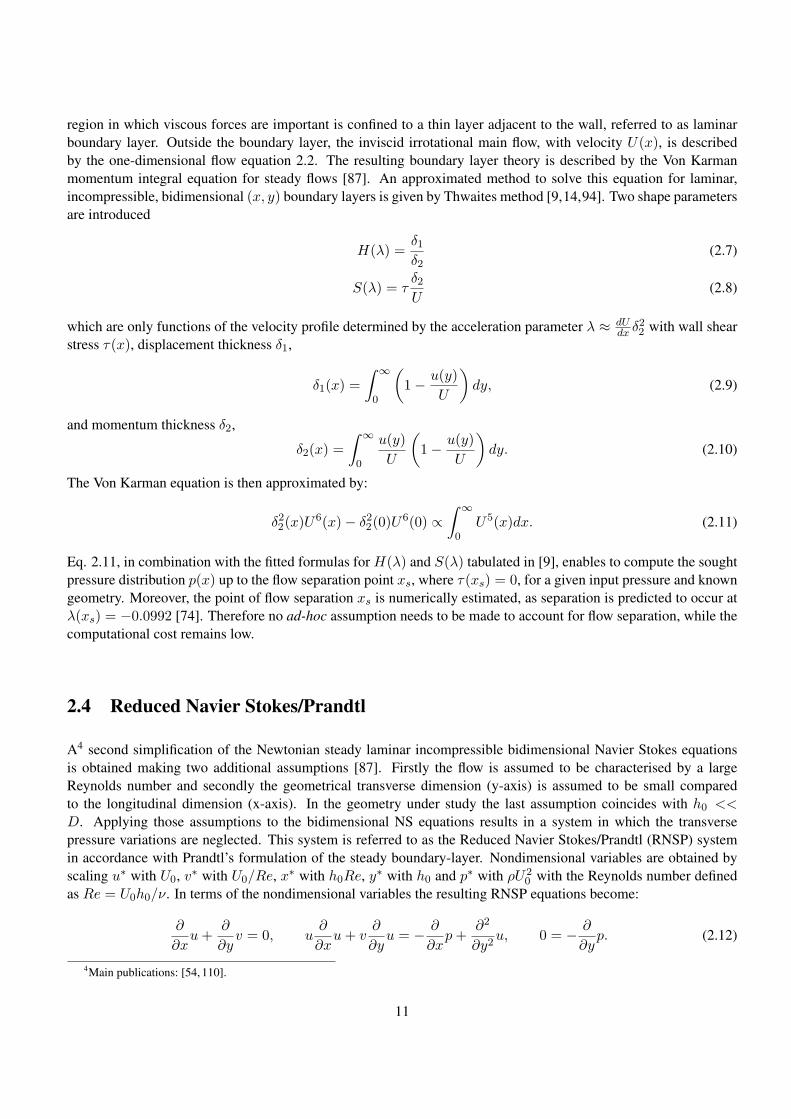
region in which viscous forces are important is confined to a thin layer adjacent to the wall, referred to as laminar

boundary layer. Outside the boundary layer, the inviscid irrotational main flow, with velocity U(x), is described

by the one-dimensional flow equation 2.2. The resulting boundary layer theory is described by the Von Karman

momentum integral equation for steady flows [87]. An approximated method to solve this equation for laminar,

incompressible, bidimensional (x, y) boundary layers is given by Thwaites method [9,14,94]. Two shape parameters

are introduced

H(λ) =δ1δ2

(2.7)

S(λ) = τδ2U

(2.8)

which are only functions of the velocity profile determined by the acceleration parameter λ ≈ dUdx δ

22 with wall shear

stress τ(x), displacement thickness δ1,

δ1(x) =

∫ ∞

0

(

1− u(y)

U

)

dy, (2.9)

and momentum thickness δ2,

δ2(x) =

∫ ∞

0

u(y)

U

(

1− u(y)

U

)

dy. (2.10)

The Von Karman equation is then approximated by:

δ22(x)U6(x)− δ22(0)U

6(0) ∝∫ ∞

0U5(x)dx. (2.11)

Eq. 2.11, in combination with the fitted formulas for H(λ) and S(λ) tabulated in [9], enables to compute the sought

pressure distribution p(x) up to the flow separation point xs, where τ(xs) = 0, for a given input pressure and known

geometry. Moreover, the point of flow separation xs is numerically estimated, as separation is predicted to occur at

λ(xs) = −0.0992 [74]. Therefore no ad-hoc assumption needs to be made to account for flow separation, while the

computational cost remains low.

2.4 Reduced Navier Stokes/Prandtl

A4 second simplification of the Newtonian steady laminar incompressible bidimensional Navier Stokes equations

is obtained making two additional assumptions [87]. Firstly the flow is assumed to be characterised by a large

Reynolds number and secondly the geometrical transverse dimension (y-axis) is assumed to be small compared

to the longitudinal dimension (x-axis). In the geometry under study the last assumption coincides with h0 <<D. Applying those assumptions to the bidimensional NS equations results in a system in which the transverse

pressure variations are neglected. This system is referred to as the Reduced Navier Stokes/Prandtl (RNSP) system

in accordance with Prandtl’s formulation of the steady boundary-layer. Nondimensional variables are obtained by

scaling u∗ with U0, v∗ with U0/Re, x∗ with h0Re, y

∗ with h0 and p∗ with ρU20 with the Reynolds number defined

as Re = U0h0/ν. In terms of the nondimensional variables the resulting RNSP equations become:

∂

∂xu+

∂

∂yv = 0, u

∂

∂xu+ v

∂

∂yu = − ∂

∂xp+

∂2

∂y2u, 0 = − ∂

∂yp. (2.12)

4Main publications: [54, 110].

11

The no slip boundary condition is applied to the lower and upper wall. Since the lower wall of the geometry of

interest corresponds to y = 0 and the distance to the upper wall is denoted with h(x) the no slip condition becomes

respectively (u(x, y = 0) = 0, v(x, y = 0) = 0) and (u(x, y = h(x)) = 0, v(x, y = h(x)) = 0). In order to

numerically solve the RNSP equations the pressure at the entrance is set to zero and the first velocity profile need to

be known (Poiseuille). There is no output condition.

2.5 Two-dimensional laminar Navier-Stokes

The5 two-dimensional continuity and Navier-Stokes equations for steady, laminar and incompressible flow are:

∂ux∂x

+∂uy∂y

= 0, (2.13)

ρ0

(

ux∂ux∂x

+ uy∂ux∂y

)

= −∂p∂x

+ µ

(

∂2ux∂x2

+∂2ux∂y2

)

, (2.14)

ρ0

(

ux∂uy∂x

+ uy∂uy∂y

)

= −∂p∂y

+ µ

(

∂2uy∂x2

+∂2uy∂y2

)

, (2.15)

where ux and uy denote the velocity component in the x and y dimension respectively [87]. For reasons of symmetry

the upper half of the flow domain is discretised in finite elements and the commercial finite element software ADINA

CFD is used as a solver [5]. The upstream pressure p0 is applied at the inlet. The no-slip boundary condition is

set to the rigid wall, while the symmetry centerline is treated as a slip wall. The mesh density is increased in the

constriction in order to accurately predict flow separation by considering vanishing wall shear stress.

2.6 Large Eddy Simulation

The6 airflow is simulated with Large Eddy Simulation (LES) for three dimensional incompressible unsteady flows

[57,84]. The spatially-filtered momentum equation (2.16) and continuity equation (2.17) are solved for a discretized

flow domain,

∂ui∂t

+∂

∂xj(uiuj) = − 1

ρ0

∂p

∂xi+ ν

∂

∂xj

(

∂ui∂xj

+∂uj∂xi

)

− ∂τij∂xj

, (2.16)

∂ui∂xj

= 0, (2.17)

where ui are the grid-scale velocity components (i = 1, 2, 3), p is the grid-scale static pressure and τij is the

subgrid scale (SGS) stress tensor. The physical parameters of the model are density ρ0 and kinematic viscosity ν.

A second-order Crank-Nicolson scheme (implicit method) is used for the discretization of the momentum equation.

The unknowns ui and p result from the decomposition of the velocity and the pressure into a resolvable (ui and p)

and subgrid scale part (u′i and p′) as:

ui = ui + u′ and p = p+ p′.

5Main publications: [20].6Main publications: [108].

12

The SGS stress tensor τij groups all terms which are not exclusively dependent on the large scale, so that:

τij = uiuj − uiuj .

The subgrid scale turbulence is modelled with the Smagorinsky closure model, which is based on the formulation of

the subgrid scale stress as:

τij −1

3τkkδij = −2νSGSSij ,

with Sij denoting the strain rate tensor and νSGS the subgrid scale eddy viscosity, which are defined by:

Sij =1

2

(

∂ui∂xj

+∂uj∂xj

)

and νSGS = (CS∆)2√

2SijSij ,

with Smagorinsky constant CS . The size of the grid filter ∆ is defined locally from the discretized volume as:

∆ =3√

Element Volume.

The Smagorinsky constant CS is calculated locally in space and time using Lilly’s least square procedure [34, 58].

The pressure field is computed from the velocity field using the fractional step method.

13

Chapter 3

Experimental conditions, measurement and

nozzles

Accurate experimental data are important for two main reasons:

1. Experimental validation of modelled quantities under controlled and reproducible conditions

2. Qualitative and quantitative characterisation to increase understanding and to motivate the model approach

In order to realise accurate in-vitro experiments the following is needed:

1. A suitable experimental setup in order to measure the quantities of interest in an accurate and reproducible

way

2. Mechanical replicas

The following section presents the range of flow conditions which are experimentally studied, some main aspects of

experimental setup and measurements and finally the used nozzles and mechanical replicas are briefly presented.

3.1 Range of flow conditions

The studied range of flow conditions, in terms of non-dimensional numbers, should cover the range of interest to

the human respiratory system. Consequently, the order of magnitude of human physiological quantities should be

considered. Relevant geometrical and flow quantities for flow through the glottis and the oral tract and pertinent with

respect to two typical phenomena such as phonation and obstructive sleep apnea (OSA) are summarised in Table 3.1.

So accounting for the properties of air the non-dimensional quantities are estimated and summarised in Table 3.2.

From the resulting order of magnitude major flow assumptions can be formulated from which a modeling approach

can be motivated.

Although estimation of the non-dimensional numbers of the flow allows to anticipate the flow behaviour, more

information is needed in order to fully characterise the flow field. Therefore, qualitative as well as quantitative

characterisation of the flow field is experimentally assessed.

14

Fluid properties of air

ρ0 Mean density 1.2kgm−3

µ0 Dynamic viscosity coefficient 1.5×10−5m2s−1

co Speed of sound 350ms−1

Oral tract

Lo Tongue length 50mm

Lt Tract length 150-190mm

Wo Pharyngeal width 15-25mm

Ho Tract heigth 10-20mm

ho Minimum aperture 1-4mm

Lt Length of teeth 1-2mm

Do Distance between teeth and lips 1.7× Lt

ht Minimum aperture at teeth 1-2mm

Dt Distance between tongue constriction and teeth 5-15mm

Uo Flow velocity 8ms−1

fo Breathing frequency 0.25Hz

Glottis

Lg Glottal length 6-9mm

Wg Glottal width 14-18mm

hg Glottal heigth 0-3mm

Ug Flow velocity 10-40ms−1

fg Fundamental frequency of oscillation 100-200Hz

Table 3.1: Some characteristic in-vivo geometrical and flow conditions for the glottis and the oral tract.

oral tract glottis assumption

aspect ratio ho/Wo << 1 hg/Wg << 1 two-dimensional

Ma2 10−4 << 1 10−2 << 1 incompressible

Sr 10−3 << 1 10−2 << 1 steady

Re 103 >> 1 103 >> 1 inviscid

Table 3.2: Nondimensional numbers and flow assumptions: aspect ratio, Mach number Ma, Strouhal number Sr, Reynolds

number Re.

3.2 Experimental setup and measurement

A general overview of the used experimental setups is schematised in Fig. 3.1.

The flow facility consists of compressed air (Copco GA7) circulating in a uniform tube with diameter 1cm for

which the volume flow rate can be imposed by means of a pressure regulator (Norgren type 11-818- 987) and a

manual valve. The valve controlled air supply is connected to a settling chamber of which the interior is tapered

with acoustical foam (SE50AL-ML). The volume of the used settling chambers varies from 0.1 up to 0.8 m3. Grids

can be used in the settling chamber in order to reduce the turbulence intensity so that the measured streamwise

turbulence intensity at the nozzle inlet is below 1%. A mechanical replica is mounted to the pressure tank. Differ-

ent sensors can be added to the setup in order to measure relevant quantities such as pressure transducers (Kulite

XCS-093), volume flow rate (TSI 4040) or hot-wire (TSI 1201-20) constant temperature anemometry (TSI IFA 300).

In complement to the experimental setup, different measurement aspects are developed as outlined in the following.

15

(C)

(B)

(A)

(D)

(a) without

(C)

(B)

(E)

(A)

(D)

(b) with

Figure 3.1: General overview of experimental setup to wich sensors can be added: (A) supplied volume airflow rate, (B)

settling chamber with (C) acoustical foam and (D) in-vitro replica. a) without and b) with air conditioning screens (E).

(a) (b) (c)

Figure 3.2: a) A sketch of the apparatus: (a) air supply, (b) pressure regulator, (c) valve, (d) mass flow meter, (e) divergent, (f)

uniform pipe, (g) convergent nozzle, (h) hot film/wire, (i) positioning system, (j) IFA 300. b) Nozzle mean exit velocity profiles

for seven volume flow rates. c) Overview of differences between four calibration methods: bulk velocity Ucal = Qmeas/S,

Johnstone’s method [50], Algo I and Algo II.

3.2.1 Hot-wire/film calibration

With1 respect to the development of the available measurement techniques and accounting for the aimed flow con-

ditions a contribution is made to the development of a simple calibration algorithm for hot film/wire allowing a joint

calibration for low (< 2m/s) and moderate (> 2m/s) flow velocities. The simple and inexpensive calibration setup

and results are illustrated in Fig. 3.2 [39].

Two simple calibration algorithms are proposed taking into account the development of the boundary layer. Algo

I uses an estimation of the displacement thickness δ1 from the measured mean velocity profile across the nozzle

exit. Algo II estimates the displacement thickness by making additional assumptions on the velocity profile in the

boundary layer and its thickness δ. As a benchmark comparison is made with the optimisation method proposed

in [50] and an estimation of the bulk velocity. Comparison of the different approaches is summarised in Table 3.3

and illustrated in Fig. 3.2.

Algo I is the most accurate since the displacement thickness δ1 is calculated from the mean velocity profile and

1Main publications: [39].

16

Procedure Measurement Velocity range Major drawback Major advantage

[50] U(y), Qmeas Ucal ≥ 3m/s accuracy loss simple to

with boundary layer implement

development

Algo I U(y), Qmeas as [50] Ucal ≥ 0.17m/s accurate spatial most accurate

exit profile for low velocities

measurement

Algo II Qmeas, U0c Ucal ≥ 0.5m/s ad-hoc coefficient reduced number

velocity data

Table 3.3: Overview of assessed hot film/wire calibration methods with exit velocity profile U(y), centerline velocity at the

nozzle exit U0c and measured volume flow velocity Qmeas.

no further assumptions are made. Therefore, the lower velocity limit of Algo I is mainly dictated by measurement

errors. The lower limit of Algo II on the other hand is dictated by the failure of the assumption of the linear growth

profile in the boundary layer. Finally, Johnstone’s method is limited by the development of the boundary layer itself.

3.2.2 Smoke visualisation

In2 complement to the pointwise spatial information of the flow field by anemometry, flow visualisation methods are

of interest to obtain a global overview of the flow field. The experimental setup is illustrated in Fig. 3.3.

Figure 3.3: Schematic overview of smoke visualisation setup: settling chamber (A), smoke generator and injector for settling

chamber (B), volume airflow rate supply (Q), pressure regulator and thermal mass flow meter (C), manual valves (D), laser

source (J), camera (E) perpendicular to the two-dimensional laser sheet (K), manual gate (G) with attachment tube (H), nozzle

(M), alternative incense burning (I). The two-dimensional illumination coincides with the plane z = W/2 and the x-axes

indicates the main flow direction.

In order to realise smoke visualisation the nozzle or mechanical replica under study is attached to a settling chamber

with volume 0.112m3. Neutrally buoyant white smoke (Steinigke Showtechnic GmbH, fluid smoke, polyglycol,

glycerol, 3-ethyleenglycol, 1.2 propyleneglycol in water double distilled water, 1.06g/cm3) is injected in the settling

chamber by means of a fog machine (Kool Light, FOG-1200E, 1200W, maximum volume flow rate 300m3/min) up

to a manual valve. Alternatively, incense is used to fill the nozzle downstream the settling chamber downstream a

closed manual gate. In both cases smoke is added in absence of airflow. Airflow is applied once sufficient smoke is

2Main publications: [37, 106].

17

injected.

Two-dimensional illumination is applied with a laser light beam. A a two-dimensional laser light beam is generated

by a class IIIb laser light source (Laserglow Technologies, LRS-0532-TFM-00200-10, 234.2mW, wavelength of

532nm and with spectral line width < 0.1nm) to which a 10 degree cylindrical lens is added. The resulting beam

has an aperture diameter of 1mm with a divergence angle < 1.5mrad.

To record the illuminated smoke pattern, a color camera (Casio, EXILIM Pro EX-F1, 6.0 million effective pixels

and a 12X optical zoom) was positioned perpendicular to the laser sheet. The back wall of the test chamber was

painted in black to ensure a good contrast with the smoke pattern. Movies are recorded at typically 300fps. So, the

time interval between consecutive images is 3.3ms. The digitised two-dimensional images are typically 512 × 384data matrices. Spatial calibration of the images is performed.

3.2.3 Acoustic insulation box

Aero-acoustic3 experiments are performed in an ordinary laboratory room equipped with a flow facility consisting

of compressed air circulating in a uniform tube with diameter 1cm for which the volume flow rate can be imposed

by means of a pressure regulator (Norgren type 11-818-987) and a manual valve. The compressor is isolated in

a separated room. The presence of the pressure regulator and airflow circuit in the room is a source of constant

broadband background noise, which can not be filtered out with standard techniques since it affects all frequencies.

Additional constant noise sources are due to the experimental procedure such as computers ventilation noise during

data acquisition. Besides unwanted noise sources inherent to the airflow facility or experimental procedure, several

punctual and random unwanted noise sources are related to inside activities of colleagues or outdoor activities of

passengers or traffic. Consequently, instead of isolating individual noise sources it has been chosen to integrate a

non expensive experimental box in the ordinary room which serves as an insulation room.

The box is inserted in the ordinary room with no acoustical treatment of volume 49.8m3 and dimensions 4.45× 4×2.80m, length × width × height. Due to the location of windows, entrance door, space required for experimental

material and instruments (such as the settling chamber for flow experiments) and manufacturing issues, the external

dimensions of the box are reduced to 2.07 × 2.10 × 2.14m, length × width × height. A two-dimensional spatial

overview of the ordinary room with insulation box is given in Fig. 3.4(a).

The insulation box is built in rigid flat wooden fiber board insulation panels with thickness 2.5cm to which acoustic

foam (SE50-AL-ML, Elastomeres Solutions) with thickness 5cm is added. The foam absorbs frequencies in the

range from 100 up to 10kHz which is ‘a-priori’ suitable for broadband noise sources such as pressure regulator, PC

ventilator, etc. The efficiency of the acoustic foam depends on the noise frequencies. Absorption and attenuation

of frequencies below 1000Hz are improved thanks to the inclusion of a basis-layer of PVC (Polyvinyl chloride

5kg/m2) to which PU Ether (Polyurethane) foam is added. Therefore, the final insulation panels of the insulation

box are three-layered - wood, PVC, foam - with a total thickness of 7.5cm as illustrated in Fig. 3.4(b). Characteristics

of the insulation box are summarised in Table 3.4.

3Main publications: [29, 105].

18

0 100 200 300 400400

300

200

100

0

y [cm]

x [c

m] P1

P2

P3

W

D0

D1

(a) room overview (b) panel section

Figure 3.4: a) Two-dimensional spatial overview of experimental room without acoustical treatment with entrance D0, room

windows W , compressed air supply ×, insulation box (dashed rectangle) equipped with 3 trapdoors P and door access D1. b)

Illustration of a section of the three-layered insulation panel.

Values & range

Internal dimensions Lx=1.92m, Ly=1.95m, Lz=1.99m

Internal volume V 7.45m3

Internal wall surface S 22.9m2

Absorbing foam 98% (αf = 0.98) 2500 < F < 10000Hz

(Elastomeres Solutions) 80% (αf = 0.8) 1000 < F < 2500Hz

(SE50-AL-ML) <80% (αf ≤ 0.8) 100 < F < 1000Hz

(linear increase)

Wall thickness 7.5cm

Table 3.4: Relevant insulation box characteristics. Internal dimensions correspond to length Lx × width Ly × height Lz .

Corresponding values of the absorption coefficient of the foam αf for different frequency ranges are indicated [1].

Three trapdoors allow access for instrumentation cables. In addition, trapdoors can be used to insert the nozzle to

be studied. Trapdoors are made of the same rigid wood panels as the box and have internal dimensions 20× 20cm,

20 × 20cm and 70 × 70cm. The trapdoors are placed at middle panel height and their positions are indicated in

Fig. 3.4(a). A wooden access door of internal dimensions 70 × 200cm (width × length) and thickness 4.5cm, is

installed to allow access inside the box for setting up the instrumentation. Acoustic foam is added to trapdoors and

access door as well. Besides insulation from outdoor noise sources, the presence of acoustic foam intends to avoid

acoustic volume resonance frequencies which depend inversely upon the characteristic lengths of the resonating

volume, indicated Lx,y,z in Table 3.4. Finally, note that, if required, the whole structure can be dismounted and

remounted.

The acoustic performance is firstly evaluated with respect to unwanted noise sources which are inherent to the

measurement procedure and to the flow facility. Signals are high-passed filtered with a fifth order Butterworth

filter with cutoff frequency 100Hz, so that the electrical network frequency of 50Hz and low frequency noises are

excluded. In addition, attenuation below 100Hz is expected to be insufficient due to the poor attenuation of the foam

as indicated in Table 3.4. All sound pressure levels are expressed in dB SPL as:

SPL = 20log10

(

prms

pref

)

, (3.1)

19

where pref = 2.10−5Pa and prms =√

1N

∑Ni=1 p

2i , with pi the ith instantaneous acoustic pressure. Sound pressure

is measured by omni directional microphones Bruel & Kjaer (type 4192) with associated pre-amplifier (B&K 4165)

and additional amplifier (0 ≤ G ≤ 50dB) and power supply (B&K 5935L) is used to perform sound measurements

in the untreated room and in the insulation box. Sounds are recorded during 10s consecutively for steady sources at

216 samples per second. The sensitivity of the microphone is determined with a calibrator (B&K4231).

The attenuation of external noise sources is quantified using a simple additive model for the sound pressure level

so that an unwanted source is considered to have no influence in case the difference between wanted and unwanted

source ∆dB is more than 25dB.

The attenuation of background noises measured inside and outside the insulation box due to airflow supply (180l/min

and 110l/min) and PC usage is given in Table. 3.5. In addition, the attenuation of human conversational speech is

Measured SPL levels

Non-treated Insulation Attenuation

Noise room (SPLR) box (SPLI ) (SPLR - SPLI )

180l/min 92dB 36dB >25dB

110l/min 82dB 36dB >25dB

PC 68dB 37dB >25dB

Voice 70dB 38dB >25dB

Reference level 36dB

Table 3.5: Performance of the insulation box for typical background noise due to the measurement procedure: measured sound

pressure levels (SPL) for air supply (180 and 110l/min) and PC usage in the non treated room (R) and in the insulation box (I).

shown. SPL-values measured in the non treated room are > 80dB for airflow supply, 68dB for computer usage and

70dB for the voice sample. Recall that the SPL level of the voice sample is within the range expected for human

conversational speech [80]. The value of computer usage and voice are from the same order of magnitude whereas

the SPL values measured for airflow supply are > 10dB larger, so that airflow supply is the most important source

of background noise during the measurements. From Table 3.5 is observed that corresponding attenuated values

measured in the insulation box approximate the reference level of 36dB. In addition, it is seen that all background

noise sources are attenuated with more than 25dB. Consequently, the attenuation of SPL for unwanted noise sources

inherent to the measurement procedure and airflow supply is satisfactory.

Next, the spectral attenuation of the insulation box is considered. Fig. 3.5(a) illustrates the attenuation with respect to

the reference level for unwanted noise sources inherent to the experimental procedure, i.e. airflow supply 110l/min

and PC usage. Both sources are broadband noises for which the spectrum covers the entire frequency domain when

measured in the non treated room. It is observed that the corresponding spectra measured inside the insulation box

match the reference level for f ≥ 300Hz and that for f < 300Hz the difference with the reference level is less

than 10dB. Note that despite the approximately square shape of the insulation box, the attenuation is independent of

its acoustical modes. Consequently, as for the attenuation in SPL, the spectral attenuation of the insulation box for

unwanted noise sources inherent to the measurement procedure and airflow supply is satisfying.

The homogeneity of measured dB SPL is estimated to have an accuracy of 4% for all frequencies in the interval

100Hz up to 10kHz. An averaged absorption coefficient α is estimated from matching modelled and measured

decay behaviour of a point source to be 0.8 ≤ α ≤ 0.95 which is in the characteristic range of the foam. From

the measured and modelled reverberation times Tr, it is observed that the insulation box is characterised by a short

20

102

103

1040

20

40

60

80

100

120

PS

D [d

B S

PL]

f [Hz]

ref.air Iair RPC IPC R

(a)

125 250 500 1000 2000 4000 8000 1600020

40

60

80

100

f [Hz]

Tr m

[ms]

Trm octave bandTrne Eyring

TrmTrs Sabine

Trm(f ≥ 2000Hz)

(b)

Figure 3.5: a) Performance of the insulation box for typical background noises due to the measurement procedure: Power

Spectral Density (PSD) for 110l/min air supply and PC usage in the non treated room (R) and in the insulation box (I). b)

Estimated mean (×) and standard deviation (vertical error bars) of the reverberation time Trm for each octave band in the

range from 89Hz up to 22.5kHz. The center frequency of each band is indicated. For comparison also the averaged measured

Trm (thin full line), the averaged high-pass filtered Trm(f ≥ 2000) (thin dashed line), modelled from Sabine’s equation Trs(thick dashed line) and modelled from Norris-Eyring equation Trne (thick full line) are indicated.

reverberation time in the range 30 ≤ Tr ≤ 60ms, which can be approximated by a constant value Tr ≈ 31 ± 2ms

for frequencies f ≥ 1400Hz as illustrated in Fig. 3.5(b).

3.3 Nozzles and mechanical replicas

Rigid and deformable nozzles and mechanical replicas with different degrees of complexity are designed to study the

flow and the influence of initial conditions on the flow development as well as the sound produced. In the following

an overview is given of the used geometries.

3.3.1 Rigid axisymmetrical nozzles

Convergent axisymmetrical nozzle

A4 convergent axisymmetrical nozzle is obtained as two matched cubics. The radius R(x) of the resulting parame-

terised axisymmetrical nozzle is defined as:

R(x) =

(

D1

2− D2

2

)

(

1− (x/L)3

(xm/L)2

)

+D2

2, x ≤ xm (3.2)

R(x) =

(

D1

2− D2

2

)

(1− x/L)3

(1− xm/L)2 +

D2

2, x > xm (3.3)

4Main publications: [30, 39].

21

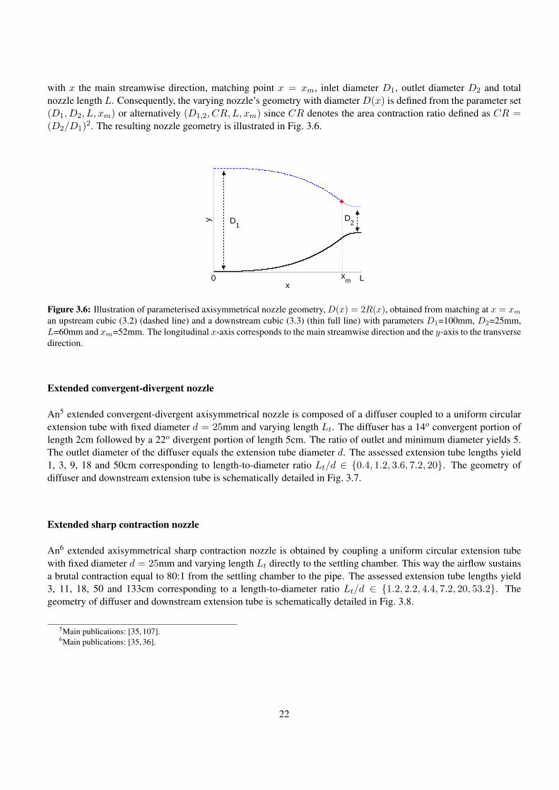
with x the main streamwise direction, matching point x = xm, inlet diameter D1, outlet diameter D2 and total

nozzle length L. Consequently, the varying nozzle’s geometry with diameter D(x) is defined from the parameter set

(D1, D2, L, xm) or alternatively (D1,2, CR,L, xm) since CR denotes the area contraction ratio defined as CR =(D2/D1)

2. The resulting nozzle geometry is illustrated in Fig. 3.6.

0 Lx

y D2D

1

xm

Figure 3.6: Illustration of parameterised axisymmetrical nozzle geometry, D(x) = 2R(x), obtained from matching at x = xman upstream cubic (3.2) (dashed line) and a downstream cubic (3.3) (thin full line) with parameters D1=100mm, D2=25mm,

L=60mm and xm=52mm. The longitudinal x-axis corresponds to the main streamwise direction and the y-axis to the transverse

direction.

Extended convergent-divergent nozzle

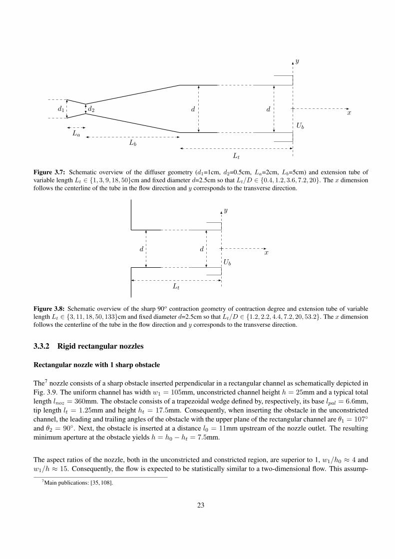
An5 extended convergent-divergent axisymmetrical nozzle is composed of a diffuser coupled to a uniform circular

extension tube with fixed diameter d = 25mm and varying length Lt. The diffuser has a 14o convergent portion of

length 2cm followed by a 22o divergent portion of length 5cm. The ratio of outlet and minimum diameter yields 5.

The outlet diameter of the diffuser equals the extension tube diameter d. The assessed extension tube lengths yield

1, 3, 9, 18 and 50cm corresponding to length-to-diameter ratio Lt/d ∈ {0.4, 1.2, 3.6, 7.2, 20}. The geometry of

diffuser and downstream extension tube is schematically detailed in Fig. 3.7.

Extended sharp contraction nozzle

An6 extended axisymmetrical sharp contraction nozzle is obtained by coupling a uniform circular extension tube

with fixed diameter d = 25mm and varying length Lt directly to the settling chamber. This way the airflow sustains

a brutal contraction equal to 80:1 from the settling chamber to the pipe. The assessed extension tube lengths yield

3, 11, 18, 50 and 133cm corresponding to a length-to-diameter ratio Lt/d ∈ {1.2, 2.2, 4.4, 7.2, 20, 53.2}. The

geometry of diffuser and downstream extension tube is schematically detailed in Fig. 3.8.

5Main publications: [35, 107].6Main publications: [35, 36].

22

d1 d2 dd x

y

La

Lb

Lt

Ub

Figure 3.7: Schematic overview of the diffuser geometry (d1=1cm, d2=0.5cm, La=2cm, Lb=5cm) and extension tube of

variable length Lt ∈ {1, 3, 9, 18, 50}cm and fixed diameter d=2.5cm so that Lt/D ∈ {0.4, 1.2, 3.6, 7.2, 20}. The x dimension

follows the centerline of the tube in the flow direction and y corresponds to the transverse direction.

dd x

y

Lt

Ub

Figure 3.8: Schematic overview of the sharp 90o contraction geometry of contraction degree and extension tube of variable

length Lt ∈ {3, 11, 18, 50, 133}cm and fixed diameter d=2.5cm so that Lt/D ∈ {1.2, 2.2, 4.4, 7.2, 20, 53.2}. The x dimension

follows the centerline of the tube in the flow direction and y corresponds to the transverse direction.

3.3.2 Rigid rectangular nozzles

Rectangular nozzle with 1 sharp obstacle

The7 nozzle consists of a sharp obstacle inserted perpendicular in a rectangular channel as schematically depicted in

Fig. 3.9. The uniform channel has width w1 = 105mm, unconstricted channel height h = 25mm and a typical total

length lnoz = 360mm. The obstacle consists of a trapezoidal wedge defined by, respectively, its base lpal = 6.6mm,

tip length lt = 1.25mm and height ht = 17.5mm. Consequently, when inserting the obstacle in the unconstricted

channel, the leading and trailing angles of the obstacle with the upper plane of the rectangular channel are θ1 = 107◦

and θ2 = 90◦. Next, the obstacle is inserted at a distance l0 = 11mm upstream of the nozzle outlet. The resulting

minimum aperture at the obstacle yields h = h0 − ht = 7.5mm.

The aspect ratios of the nozzle, both in the unconstricted and constricted region, are superior to 1, w1/h0 ≈ 4 and

w1/h ≈ 15. Consequently, the flow is expected to be statistically similar to a two-dimensional flow. This assump-

7Main publications: [35, 108].

23

lup lpal l0

lnoz

lt

ht

h

h0

θ1 θ2

w1

y

xz

x = 0 x

y = 0

y

Figure 3.9: Schematic representation of the nozzle. The x-axis corresponds to the main flow direction and the y-axis to the

transverse direction perpendicular to the flat wall.

tion was experimentally verified by hot-film anemometry measurements. The contraction ratio h0/h yields ≈ 3.3resulting in a 70% obstruction degree at the obstacle. The ratios of 1) the obstacle length lpal and 2) the channel

downstream the constriction l0 to the minimum aperture yield lpal/h = 0.88 and l0/h = 1.47.

Rectangular nozzle with 1 gradual and 1 sharp obstacle

The8 rectangular nozzle with 1 gradual and 1 sharp obstacle is shown in Fig. 3.10. The rigid ‘in-vitro’ replica consists

of two constrictions, C1 and C2, inserted in a uniform rectangular channel. The unconstricted channel has length

L0 = 180mm, height h0 = 16mm, width w = 21mm and aspect ratio w/h0 = 1.3. The shape of both constrictions

C1 and C2 is fixed. Their lengths in the x-direction yield l1 = 30mm for C1 and l2 = 3mm for C2. The aperture

h1 is fixed to 3mm, which corresponds to a constriction degree of 81%. The distance of the trailing edge of C2 to

the channel exit, L2, is fixed to 6mm. The distance of the trailing edge of C1 with respect to the channel exit, L1,

can be varied as well as aperture height h2 of constriction C2. Therefore, besides the inlet height h0, the pressure

distribution is determined by the set of geometrical parameters {h1, L1, h2} among which L1 and h2 can be varied.

In order to validate the pressure drop, three pressure taps are assessed at positions p0 = 30mm, p1 = 160mm and

p2 = 173mm from the channel inlet. The position of the pressure taps is fixed to prevent leakage.

Constriction shapes: fixed and movable

Two9 sets of uniform and round constriction shapes are available as shown in Fig. 3.11(a). Constrictions are mounted

by means of an adjustement screw in a rectangular holder of fixed width w = 25mm, illustrated in Fig. 3.11(b), to

which side walls are added covering at least the constricted portion. Note that a downstream channel of varying

length and geometry can be added. The adjustement screws allows to vary the minimum aperture h.

To each constriction of length 10mm a step motor (Radiospare L92121-P2) can be attached so that its move-

ment along the y-axis can be controlled (LabView, National Instruments). A symmetrical oscillatory movement,

y(t) = A sin(2πFt), is imposed to both constrictions for which both frequency F and amplitude A can be varied.

8Main publications: [24, 101, 109].9Main publications: [17, 19].

24

p2

p1p0

0 x0

y

p0 = 30mm p1 = 160mm p2 = 173mm

× × ×

h0 = 16mm

h1 = 3mm

h2

L = L1 − 9mm

L2 = 6mm

L1

L0 = 180mm

C1

C2

l1 = 30mm

l2 = 3mm

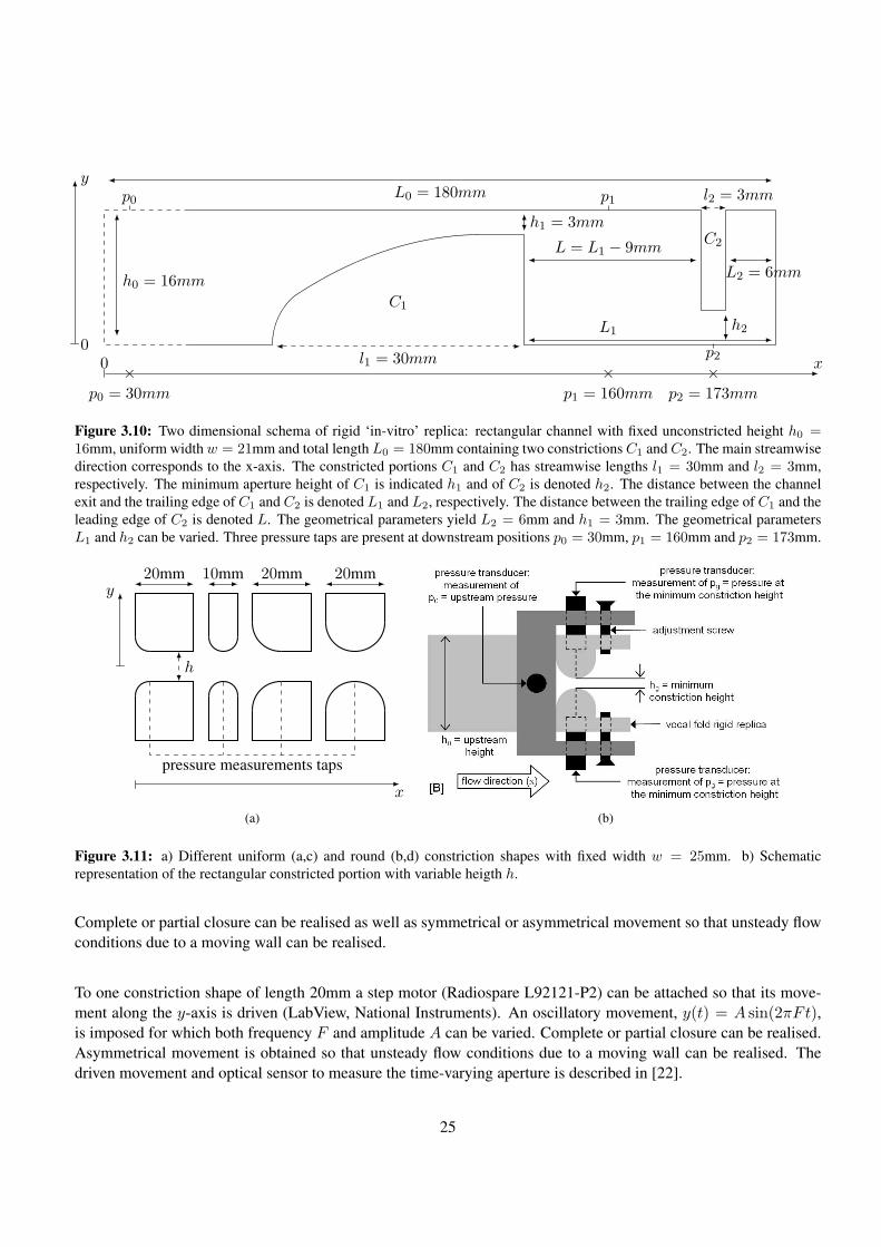
Figure 3.10: Two dimensional schema of rigid ‘in-vitro’ replica: rectangular channel with fixed unconstricted height h0 =16mm, uniform widthw = 21mm and total length L0 = 180mm containing two constrictions C1 andC2. The main streamwise

direction corresponds to the x-axis. The constricted portions C1 and C2 has streamwise lengths l1 = 30mm and l2 = 3mm,

respectively. The minimum aperture height of C1 is indicated h1 and of C2 is denoted h2. The distance between the channel

exit and the trailing edge of C1 and C2 is denoted L1 and L2, respectively. The distance between the trailing edge of C1 and the

leading edge of C2 is denoted L. The geometrical parameters yield L2 = 6mm and h1 = 3mm. The geometrical parameters

L1 and h2 can be varied. Three pressure taps are present at downstream positions p0 = 30mm, p1 = 160mm and p2 = 173mm.

20mm 10mm 20mm 20mm

h

pressure measurements taps

x

y

(a) (b)

Figure 3.11: a) Different uniform (a,c) and round (b,d) constriction shapes with fixed width w = 25mm. b) Schematic

representation of the rectangular constricted portion with variable heigth h.

Complete or partial closure can be realised as well as symmetrical or asymmetrical movement so that unsteady flow

conditions due to a moving wall can be realised.

To one constriction shape of length 20mm a step motor (Radiospare L92121-P2) can be attached so that its move-

ment along the y-axis is driven (LabView, National Instruments). An oscillatory movement, y(t) = A sin(2πFt),is imposed for which both frequency F and amplitude A can be varied. Complete or partial closure can be realised.

Asymmetrical movement is obtained so that unsteady flow conditions due to a moving wall can be realised. The

driven movement and optical sensor to measure the time-varying aperture is described in [22].

25

Asymmetrical constriction

An10 asymmetrical rectangular constriction is obtained by placing a rigid half cylinder with diameter D = 49mm

inside a rectangular uniform pipe as shown in Fig. 3.12. The minimum aperture can be varied. Pressure taps are

foreseen along the flat bottom plate of the constriction.

h0 = 34mm

D = 49mm

h

x

y

pressure taps

(a)

h0 = 25mm

D = 49mm

h

x

y

pressure taps

(b)

Figure 3.12: Asymmetrical rigid nozzles a) fixed width w = 34mm and b) fixed width w = 25mm.

3.3.3 Deformable mechanical replicas

Deformable asymmetrical constriction

A11 deformable asymmetrical constriction which can be schematically presented by Fig. 3.12(b) is obtained by

replacing the rigid cylinder by a deformable portion. The deformable portion consists in a hollow cylinder which

can be filled with water and covered with latex (Piercan Ltd) as illustrated in Fig. 3.13. Mechanical properties of the

deformable portion are varied by changing the internal water pressure in the cylinder.

The transverse deformation of the mechanical replica due to the interaction with an upstream airflow resulting in

partial closure is illustrated in Fig. 3.14 for a fixed upstream pressure. In addition, the longitudinal deformation is

illustrated by a simple dye deposit experiment in Fig. 3.15. It is observed that a complete closure can be reproduced

as well as an important movement of the deformable portion in the airflow direction during closure.

Deformable symmetrical constriction

A12 symmetrical deformable constriction is obtained by two connected latex tubes (Piercan Ltd) of 11mm diameter.

The tubes are mounted on two metal cylinders with diameter 12mm for which the metal is removed over half the

diameter for a length of 40mm. The latex tubes are filled with water supplied through a central duct of 3mm

diameter connected to a water column. The same way as for the asymmetrical deformable constriction the height

10Main publications: [110].11Main publications: [15, 16, 102].12Main publications: [17, 18, 104].

26

(a) cover and support (b) upper cylinder (c) support and flat pate

(d) upper view support (e) mounting (f) frontal view at downstream end

Figure 3.13: Mounting of the deformable asymmetrical mechanical replica schematised by Fig. 3.12(b): a) latex cover and

rigid support, b) resulting deformable upper cylinder, c) rigid support and removable flat bottom plate, d) upper view of rigid

support, e) mounting the deformable portion, and f) mounted replica.

(a) instant 1 (b) instant 2

(c) instant 3 (d) instant 4

Figure 3.14: Illustration of transverse deformation at consecutive time instants.

of the water column, and so internal pressure in the latex tubes, is controllable. The latex tubes are fixated in a

metal block in order to prevent leakage. Increasing or decreasing the internal pressure by lifting or lowering the

water column implies a change in initial aperture between the two tubes and consequently the two parameters are

related in a unique way. In order to vary the initial aperture and the internal pressure in a non-unique way an

equal set of uniform rectangular metal shims with fixed length (12mm), fixed width (16mm) and variable thickness

can be inserted at the outer borders between the upper and lower portion of the replica separating both latex tube

holders to a user controlled extent. This way the initial center aperture at rest is varied from complete closure to

a maximum aperture of 10mm. As a consequence the internal pressure and initial aperture are no longer defined

27

(a) dye suppression on latex cylinder (b) dye deposit on rigid flat plate

Figure 3.15: Illustration of longitudinal deformation from dye deposit of the deformable upper part: a) on the rigid flat plate,

b) after a fluid-structure interaction illustrating contact or a total collapse of the deformable tongue replica shown in 3.13 as

well as an important movement in the flow direction.

by a 1-1 relationship. Instead different initial apertures are associated with each internal pressure. The deformable

symmetrical constriction is illustrated in Fig. 3.16 .

(a) (b)

Figure 3.16: a) Schematic representation of symmetrical deformable replica. Latex tubes [a] are connected to water column

[c] enabling to impose the internal pressure Pin. Each latex tube is mounted in a metal block [b,b’] by means of fixation screws

[e]. The initial geometrical configuration in absence of airflow was characterized by the center aperture h0c . h0c is varied 1) by

imposing internal pressure Pin and 2) by inserting a set of shims [d] between the outer parts of the upper and lower portion of

the mounting block. In absence of shims the aperture is minimal [d’]. b) Photographic illustration.

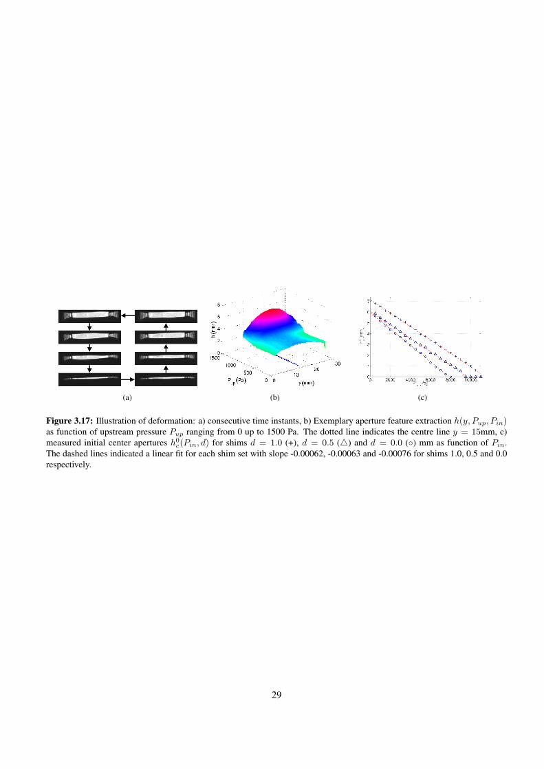
The transverse deformation of the deformable symmetrical constriction due to auto-oscillation of the deformable

constriction under influece of a given upstream pressure is illustrated in Fig. 3.17(a). The dependence of the defor-

mation on the applied upstream pressure is illustrated in Fig. 3.17(b) and on the internal water pressure in absence

of airflow is shown in Fig. 3.17(c).

28

(a) (b) (c)

Figure 3.17: Illustration of deformation: a) consecutive time instants, b) Exemplary aperture feature extraction h(y, Pup, Pin)as function of upstream pressure Pup ranging from 0 up to 1500 Pa. The dotted line indicates the centre line y = 15mm, c)

measured initial center apertures h0c(Pin, d) for shims d = 1.0 (+), d = 0.5 (△) and d = 0.0 (◦) mm as function of Pin.

The dashed lines indicated a linear fit for each shim set with slope -0.00062, -0.00063 and -0.00076 for shims 1.0, 0.5 and 0.0

respectively.

29

Chapter 4

Characterisation of jet development

Some examples of qualitative and quantitative characterisation of jet development at the exit of some of the nozzles

described in the previous chapter are summarised in the following.

4.1 Round free jet development

Despite the reported universal behaviour for an axisymmetric jet, the influence of initial conditions and geometry

on axisymmetrical jet development is put forward from analytical arguments, numerical simulations as well as ex-

perimental evidence. In among others [31, 32] it is shown analytically that the averaged equations of motion for a

number of flows admit to more general similarity solutions that retain a dependence on both the Reynolds number

and the initial conditions. Consequently, decay rate constant K and the virtual origin depend on conditions at the

tube outlet. Those analytical findings were in agreement with earlier experimental results of [41, 59, 71, 113] illus-

trating among others the influence of initial conditions on the development of coherent structures and consequently

on the spreading rate for Reynolds numbers Re > 104. More recent experimental studies confirmed these earlier

findings by putting into evidence the influence of initial conditions as well as nozzle geometry features: e.g. nozzle

diameter [63], nozzle shape [67, 76], boundary layer thickness [47, 82], exit velocity profile [6, 115], exit grid [13]

and Reynolds number [75, 78]. In addition, the influence of the initial velocity profile at the tube exit is shown by

means of numerical simulations [11].

Most of the cited studies deal with Reynolds numbers ≥ 104. Nevertheless, in particular jets associated with moder-

ate Reynolds numbers, Re < 104, appear to be sensitive to initial conditions [32, 63]. Experimental studies dealing

with the influence of diameter d and inital mean velocity U0 on the centerline velocity decay of axisymmetric jets

with uniform initial outlet profile at moderate Reynolds numbers are presented in [63, 71]. Those studies show that

the centerline velocity decay coefficient decreases and the half-width spread angle increases for decreasing outlet

Reynolds numbers. Moreover in [63] it is concluded that the velocity decay coefficients are best correlated by the

nozzle centerline velocity at the outlet U0. Both studies [63, 71] dealt with ASME Standard Long Radius Nozzles

with diameters 0.1524, 0.0758 and 0.0401m for Reynolds numbers of order Re ≈ 104 and turbulence intensities

below 9%. Obviously, data for moderate Reynolds numbers, Re < 104 and non-standard nozzle geometries are less

studied.

30

4.1.1 Extended convergent-divergent nozzle

The1 spatial jet development is sought for given initial momentum M0 = πd2U2b /4, i.e. constant tube diameter

d = 25mm and constant initial bulk velocity Ub = 4.4m/s resulting in moderate Reynolds Re = 7350 and low

Mach number flow of order 10−2. The influence of extension tube length Lt on the velocity profile at the tube outlet

and on the resulting jet development is sought. Jet development is measured by scanning the velocity field with

hot-film single sensor anemometry from the tube exit up to 20 times extension tube diameter d.

The following observations are made:

I) Both the shape of mean (Blasius to top-hat) and fluctuating portion (rms 6-50%) of the initial velocity profile at

the tube outlet are severly altered as the ratio Lt/d decreases reflecting the influence of the upstream diffuser on

initial conditions. Consequently, for the range of flow and geometrical conditions studied, varying the extension

length downstream a convergent-divergent diffuser is a natural way to vary initial conditions. Initial conditions are

illustrated in Fig. 4.1.

(a) U/U0 (b) u′/U0

Figure 4.1: Initial conditions at tube exit (x/d < 0.01) for Lt/d 0.4 (×), 1.2 (◦), 3.6 (△), 7.2 (+) and 20 (⊲): a) normalised

mean velocity U/U0 and Blasius profile (full line) b) normalised rms of velocity u′/U0.

II) With respect to centerline and transverse mean velocity modelling it is shown that self-similar models can be

applied regardless the initial conditions. Nevertheless, established relationships between common model parameters

such as the centerline velocity decay K ∼ U0 and the spreading rate S ∼ 1/U0 are inversed as the initial turbulence

level increases from 12 up to 27%. Additional data in this turbulence range should be considered to establish a region

for which the relationship K ∼ U0 is inversed due to high initial turbulence levels which favours velocity decay.

Moreover, additional data might allow the relationship of the centerline velocity decay with U0 to be extended to

account for the initial turbulence level. With respect to upper airway geometries and flow conditions, self-similar jet

models can be applied although parameters need to be adapted depending on the initial turbulence level and initial

mean velocity U0. Application of self-similar jet models is illustrated in Fig. 4.2.

III) Comparing transverse and centerline turbulence statistics, i.e. rms and skewness, for all assessed extension

tubes illustrates the difference in shear layer development. Centerline turbulence statistics yield asymptotic values

for x/d ≥ 8 for which the value depends on the initial turbulence level and so on Lt/d. The difference in shear

layer development is also observed in the one-dimensional velocity spectrum. The spectra exhibit a common inertial

1Main publications: [35, 107].

31

(a) centerline (b) transverse Lt/d = 0.4 (c) transverse Lt/d = 20

Figure 4.2: a) Inverse normalised longitudinal mean centerline velocities compensated for the self-similar law KU0/Uc : Lt/d0.4 (×), 1.2 (◦), 3.6 (△), 7.2 (+) and 20 (⊲). The potential core xp in the self-similar representation is indicated for Lt/d 3.6

(△), 7.2 (∗) and 20 (⊲) and b,c) Similarity representation of transverse normalised axial mean velocity profiles U/Uc for x/d1.6 (⋆), 3.2 (⋄), 4 (+), 4.8 (×), 6.4 (◦), 8 (⊲), 12 (△), 16 (�).

range of limited extent due to the moderate Reynolds number followed by a decay range which depends on Lt/din accordance with the difference in turbulence development. Shear layer development and spectra are illustrated in

Fig. 4.3.

(a) (b)

Figure 4.3: a) Normalised transverse rms velocity at x/d = 1.6 for Lt/d 0.4 (×), 1.2 (◦), 3.6 (△), 7.2 (+) and 20 (⊲) and b)

One dimensional velocity spectra at x = 1.6d at maximum shear stress position for Lt/d 0.4 (×), 1.2 (◦), 3.6 (△), 7.2 (+) and

20 (⊲) where k = ωd/Uc(x) denotes the dimensionless wavenumber.

IV) Since a gradient-transport model is generally assumed to hold near the centerline of an axisymmetrical jet,

turbulent viscosity near the centerline is estimated in order to assess the shear stresses in this region as well as to

obtain a qualitative estimation away from the centerline. Two-component velocity measurements are required to

obtain an accurate measurement of the shear stresses in order to validate the shear stress estimations over a large

range of initial turbulence intensities. Nevertheless, the current turbulent viscosity and shear stress estimations

provide a qualitative estimation which might be applied in modelling. Relevant quantities are illustrated in Fig. 4.4.

32

(a) (b) (c)

Figure 4.4: a) Spreading rates S(Lt/d), 0.094 (dotted) and 0.086 (full) are derived from [48] and Gaussian function with

n = 94, b) Experimental turbulence viscosity νT (Lt/d) at x/d 1.6 (⋆), 3.2 (⋄), 4.8 (×), 8.0 (⊲) and 16 (�) and c) Normalised

estimated shear stresses at x/d = 1.6 for Lt/d 0.4 (×), 1.2 (◦), 3.6 (△), 7.2 (+) and 20 (⊲).

4.1.2 Extended sharp contraction nozzle

The2 motivation to study jet flow at the exit of an extended sharp contraction nozzle follows the motivation given

earlier for the extended convergent-divergent nozzle. Former investigations are essentially conducted for industrial

purposes and reported results are obtained for high bulk Reynolds number flow, typically 104 or higher, and for geo-

metrical configurations either aiming optimal nozzle design or developed pipe flow for which the length-to-diameter

ratio exceeds 40 with well controlled flow entrance to the nozzle. Although studies at low Reynolds number have

been conducted [2, 3, 53] few information is available of the influence of the tube extension length downstream an

sharp constraction. Varying the extension length is a simple flow control device. Consequently, increased under-

standing of the flow behaviour is required to describe flow development and vortex generation in the mixing layer of

the round jet.

So the effect of a sharp contraction coupled with a downstream circular tube with varying length-to-diameter ratio is

sought for different moderate bulk Reynolds numbers 1000 < Reb < 1.2×104. Hot-film anemometry measurements

and smoke visualisation are reported here in order to evaluate the effects of two length-to-diameter ratios L/D ∈{1.2, 53.2}, coupled with sharp angles, over 19 Reynolds numbers ranging from 1131 to 11320. The experimetal

setup and smoke visualisation are illustrated in Fig. 4.5. Main results shown deal with the mean velocity exit profile,

the turbulence intensity, the centerline velocity decay rates, the virtual origin in the near field of the jet (x/D < 20)

and the generation of coherent structures.

The following observations are made:

Despite significant differences between the assessed length-to-diameter ratios, similarities in the overall jet behaviour

are found:

• For Reynolds number Reb > 4527, the potential core xpc is found to increase with Reynolds number. Al-

though this evolution is in opposition with some previous studies on smooth contraction nozzle shapes, a good

overall agreement with the models developed by [42,86] generally applied/valid for higher Reynolds numbers,

2Main publications: [35, 36].

33

(a) (b)

Figure 4.5: a) Schematic view of the setup during anemometry [a] air compressor, [b] pressure regulator, [c] valve, [d] volume

flow rate, [e] settling chamber, [f] pipe section, [g] hot film, [h] IFA-300 TSI, [i] positioning system carrying the hot film.

b) Instantaneous images of jet flows for the two assessed length-to-diameter ratios L/D = 1.2 (1) and L/D = 53.2 (2) for

Reynolds numbers Reb 1132 (1-2a), 1697 (1-2b), 2263 (1-2c), 2824 (1-2d), 3961 (1-2e), 11317 (1-2f).

is observed as shown in Fig. 4.6(a).

• The velocity decay constant K increases with Reynolds number Reb due to a reduced flow mixing with the

surrounding flow illustrated in Fig. 4.6(b).

• As Reynolds number Reb is increased, the virtual origins x0 of the jet flow moves continuously upstream

leading to the observation of negative values analysed as the consequence of back flow.

• The initial centerline turbulence intensity is decomposed into two regimes in function of the Reynolds number

Reb as shown in Fig. 4.6(c). In the range 1132 < Reb < 2200 the initial centerline turbulence intensity

increases with Reynolds numbers before continuously decreasing for higher Reynolds numbers towards an

asymptotic value as observed in literature.

Nevertheless, the applied length-to-diameter ratio L/D downstream the coupled sharp edged tube inlet is seen to

affect:

• The initial mean velocity profiles at the tube exit, illustrated in Fig. 4.7(a), shift from a Poiseuille profile to

a 1/7 power law velocity profile as the Reynolds Reb number is increased for L/D = 53.2. The observed

34

(a) (b) (c)

Figure 4.6: For L/D = 1.2 and L/D = 53.2: a) Normalised potential core extent xpc/D as function of Reynolds number

Reb. b) Normalised velocity decay constant K as function of Reynolds number Reb. c) Initial centerline turbulence intensity

profiles TU,0(y/D = 0, x/D = 0)(Reb, L/D) as function of Reynolds number Reb.

shift is in accordance with previous studies. For the smallest ratio L/D = 1.2 a trapezoidal velocity profile is

generated at the tube exit for all assessed Reynolds numbers Reb .

• The initial transverse turbulence intensity profile at the tube exit, illustrated in Fig. 4.7(b), shows a complex

variation for L/D = 1.2. In the wall vicinity a region of turbulence dissipation is observed at low Reynolds

numbers Reb.

• For L/D = 1.2, the longitudinal mean jet centerline velocity in the near field, 0 < x/D < 5, exhibits a

singular behaviour with a velocity evolution decomposed into 2 phases: a strong velocity decrease followed

by a constant velocity portion shown in Fig. 4.8(a). In parallel, the turbulence intensity Tu presents a peak

intensity in the range 1620 ≤ Reb ≤ 4527 illustrated in Fig. 4.8(b). The observation of such phenomena is

similar to [99], where the jet issues from a smooth convergent nozzle. Smoke visualisation illustrates the the

formation of toroidal ring vortices in this range of Reynolds numbers shown in Fig. 4.5(b). As the Reynolds

number Reb is increased we observe the formation of a secondary vortex in the tail of the first one due to the

upstream presence of sharp edges, and a pairing phenomenon. This observation is confirmed by the observed

velocity power spectra for which a large and a thin peak is found. Some spectra are illustrated if Fig. 4.9. In

case of L/D = 53.2, the mean centerline velocity decreases slowly and continuously, with no hump in the

turbulence intensity.

(a) (b)

Figure 4.7: For L/D = 1.2 and L/D = 53.2: a) Mean velocity profiles and b) Turbulence intensity profiles.

35

(a) (b)

Figure 4.8: For L/D = 1.2 (upper) and L/D = 53.2 (bottom): a) Normalised mean centerline mean velocity in the near field

downstream region 0 < x/D < 5. b) Centerline turbulence intensity TU .

(a) (b)

Figure 4.9: For Reynolds numbers Reb = {1132, 1697, 2263, 2824, 3961, 11317}: a) Power spectra at the position (x/D =0, y/D = 0.5). The spectra for L/D = 53.2 are shifted one decade downwards with respect to L/D = 1.2. b) Power spectra

of centerline of velocity signals for L/D = 1.2 at five downstream positions x/D = {1(×), 2(�), 3(>), 4(◦), 5(+)}. Every

spectrum is shifted one decade downwards with respect to the previous.

4.1.3 Mean jet decay model parameters

The3 time averaged turbulent jet flow mixing region is schematically divided into three parts: an initial near field

region downstream the exit, a transition region and a self-preserving far field region further downstream. In this third

zone, the axisymmetrical jet flow is typically modelled by a simple decay equation [87].

U c(x) =U0KD

x− x0, (4.1)

with U c denoting the mean centerline velocity, U0 the centerline mean velocity at the exit, K the mean centerline

velocity decay coeffiecient and x0 the virtual origin as illustrated in Fig. 4.10. The decay model is illustrated for

the convergent-divergent nozzle in Fig. 4.2(b) where the mean centerline velocy compensated for the self-similar

decay model is plotted. The influence of inlet geometry, tube extension L/D and Reynolds number Reb on the flow

3Main publications: [35, 36, 38].

36

Figure 4.10: Illustration of the self-similar jet decay model and its parameters: decay constant K and virtual origin x0.

development and therefore on the model coefficients is shown in the previous section and findings are summarised

in Table 4.1 for an abrupt reduction. In case the tube extension is preceeded by a diffuser the influence of the tube

extension length L/D is enforced compared to an abrupt reduction and the observed turbulence intensity TU and

decay constant K are seen to depend mainly on the tube extension length L/D [35].

Table 4.1: Overview of influence of Reynolds number Reb and extension length L/D on jet development: intial velocity

profile, turbulence intensity TU , vortex strucutes, model coefficients (K,x0).

Sharp extended nozzle

Reb L/D

Singular initial velocity profilesL/D

(reducion of boundary layer)

Turbulence intensity TU,0 Reb L/DTurbulence intensity peak TU 1131 < Reb < 4000

Vortex structures Reb L/D

Model coefficients (K,x0) Reb

In Table 4.2 values of the model coefficients (K,x0) reported in literature are compared to values from the sharp

extended nozzle for Reb = 11318 illustrating that for the largest experimentally assessed Reb the decay constant Kis within the range reported in literature.

4.2 Rectangular free jet development

4.2.1 Rectangular nozzle with 1 sharp obstacle

Flow4 through asymmetrical nozzle geometries occurs naturally in different aspects of daily life. Despite their

relevance most research efforts deal with well designed symmetrical nozzles under impulse of aeronautic applica-

tions [8, 46, 69]. Moreover, the same way as for axisymmetrical nozzles, most research on plane, wall or slot jet

studies deals with large Reynolds numbers (Reb ≫ 5000), e.g. tabled overviews reported in [40, 41, 55, 88], data

for low to moderate Reynolds number flows are few. A recent study concerning the influence of Reynolds number

(1500 < Reb < 16500) on orifice plane jet development points out that the effect on the mean and turbulent field is

4Main publications: [106].

37

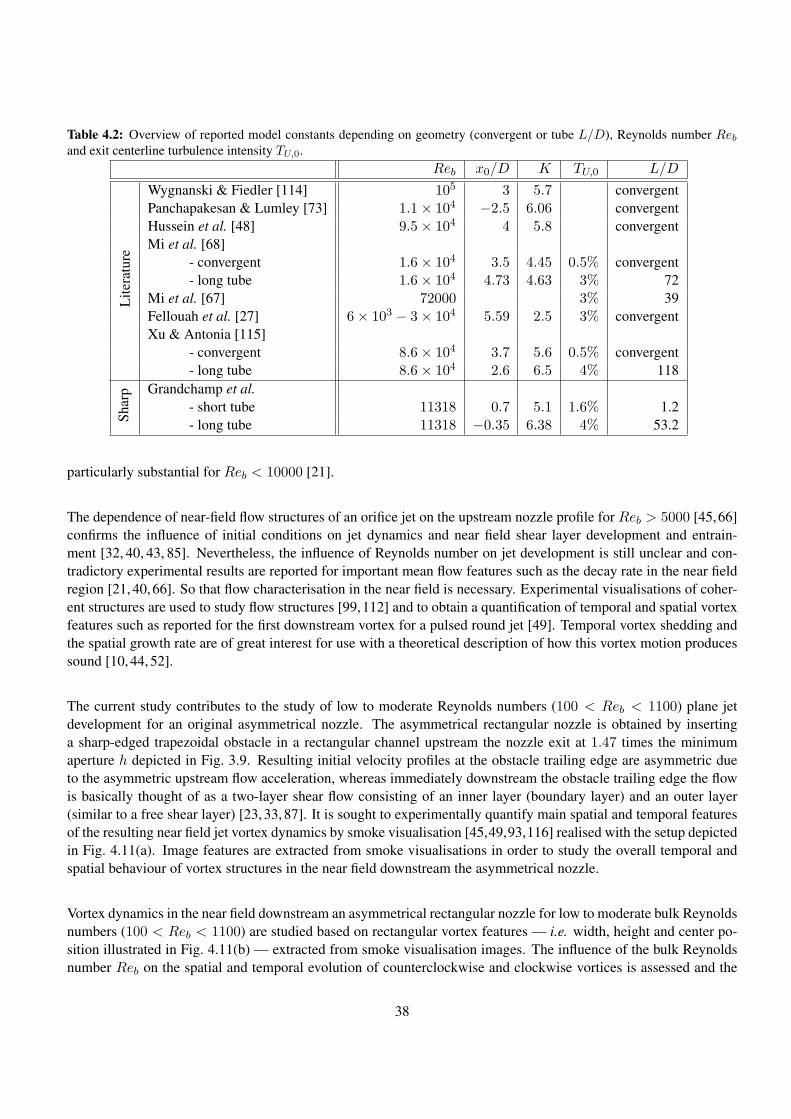
Table 4.2: Overview of reported model constants depending on geometry (convergent or tube L/D), Reynolds number Reband exit centerline turbulence intensity TU,0.

Reb x0/D K TU,0 L/D

Lit

erat

ure

Wygnanski & Fiedler [114] 105 3 5.7 convergent

Panchapakesan & Lumley [73] 1.1× 104 −2.5 6.06 convergent

Hussein et al. [48] 9.5× 104 4 5.8 convergent

Mi et al. [68]

- convergent 1.6× 104 3.5 4.45 0.5% convergent

- long tube 1.6× 104 4.73 4.63 3% 72

Mi et al. [67] 72000 3% 39

Fellouah et al. [27] 6× 103 − 3× 104 5.59 2.5 3% convergent

Xu & Antonia [115]

- convergent 8.6× 104 3.7 5.6 0.5% convergent

- long tube 8.6× 104 2.6 6.5 4% 118

Shar

p Grandchamp et al.

- short tube 11318 0.7 5.1 1.6% 1.2

- long tube 11318 −0.35 6.38 4% 53.2

particularly substantial for Reb < 10000 [21].

The dependence of near-field flow structures of an orifice jet on the upstream nozzle profile for Reb > 5000 [45,66]

confirms the influence of initial conditions on jet dynamics and near field shear layer development and entrain-

ment [32, 40, 43, 85]. Nevertheless, the influence of Reynolds number on jet development is still unclear and con-

tradictory experimental results are reported for important mean flow features such as the decay rate in the near field

region [21, 40, 66]. So that flow characterisation in the near field is necessary. Experimental visualisations of coher-

ent structures are used to study flow structures [99,112] and to obtain a quantification of temporal and spatial vortex

features such as reported for the first downstream vortex for a pulsed round jet [49]. Temporal vortex shedding and

the spatial growth rate are of great interest for use with a theoretical description of how this vortex motion produces

sound [10, 44, 52].

The current study contributes to the study of low to moderate Reynolds numbers (100 < Reb < 1100) plane jet

development for an original asymmetrical nozzle. The asymmetrical rectangular nozzle is obtained by inserting

a sharp-edged trapezoidal obstacle in a rectangular channel upstream the nozzle exit at 1.47 times the minimum

aperture h depicted in Fig. 3.9. Resulting initial velocity profiles at the obstacle trailing edge are asymmetric due

to the asymmetric upstream flow acceleration, whereas immediately downstream the obstacle trailing edge the flow

is basically thought of as a two-layer shear flow consisting of an inner layer (boundary layer) and an outer layer

(similar to a free shear layer) [23, 33, 87]. It is sought to experimentally quantify main spatial and temporal features

of the resulting near field jet vortex dynamics by smoke visualisation [45,49,93,116] realised with the setup depicted

in Fig. 4.11(a). Image features are extracted from smoke visualisations in order to study the overall temporal and

spatial behaviour of vortex structures in the near field downstream the asymmetrical nozzle.

Vortex dynamics in the near field downstream an asymmetrical rectangular nozzle for low to moderate bulk Reynolds

numbers (100 < Reb < 1100) are studied based on rectangular vortex features — i.e. width, height and center po-

sition illustrated in Fig. 4.11(b) — extracted from smoke visualisation images. The influence of the bulk Reynolds

number Reb on the spatial and temporal evolution of counterclockwise and clockwise vortices is assessed and the

38

influence of the asymmetry is outlined.

The following observations are made:

I) Spatial characterisation of mean streamwise and transverse center positions of 1 up to 3 counterclockwise and

clockwise vortices shows 1) an asymmetry of the spatial distribution of the mean center coordinates between coun-

terclockwise and clockwise vortices and 2) a reduction of the spatial life-span of the vortices from x/h < 15 to

x/h < 5 as Reb increases in the range 100 < Reb < 1100. The observed asymmetry is most pronounced for

the first vortices situated immediately downstream the nozzle exit stressing the influence of the asymmetry of the

nozzle on the flow development. This finding encourages further studies of the influence of the aperture as well as

the obstacle placement with respect to the nozzle exit on the spatial jet vortex dynamics and associated transition to

turbulence.

II) The width-to-height ratio R < 1 for the first counterclockwise as well as first clockwise vortex indicates that

vortices immediately downstream the nozzle exit are stretched in the transverse direction independently of Reynolds

number Reb. As the vortices are convected downstream R increases, i.e. vortices are stretched in the streamwise

direction, with a rate depending on the Reynolds number illustrated in Fig. 4.12.

III) The vortex shedding rate fv is found to increase linearly with bulk Reynolds numberReb. From this relationship

the Strouhal number is seen to increase with Reynolds number Reb and an analytical approximation for St(Reb) is

proposed depending on the linear regression parameters (α, β) describing fv ∝ Reb and minimum aperture h. The

findings are illustrated in Fig. 4.13.

y zx Q

A

C

NLB

LSB

(a)

streamwise x

transverse y

time t

××center

width

height

(b)

Figure 4.11: a) Schematic representation of the experimental setup for smoke visualisation: 1) settling chamber (A) of volume

0.112m3 with dimensions 56 × 50 × 40cm to which the nozzle (N) represented in Fig. 3.9 is attached, 2) smoke generation

and injection (B), 3) volume airflow rate supply (Q) with pressure regulator and thermal mass flow meter, 4) laser source

(LS) with cylindrical lens (θ3 = 10◦), 5) high speed camera (C) perpendicular to the laser sheet (LB). The laser source (LS)

and camera (C) are mounted on a three-dimensional rail system. The x-axis indicates the main flow direction. b) Schematic

representation of sought spatial vortex features derived from an enveloping rectangle (center position, height and width) and

their time evolution.

39

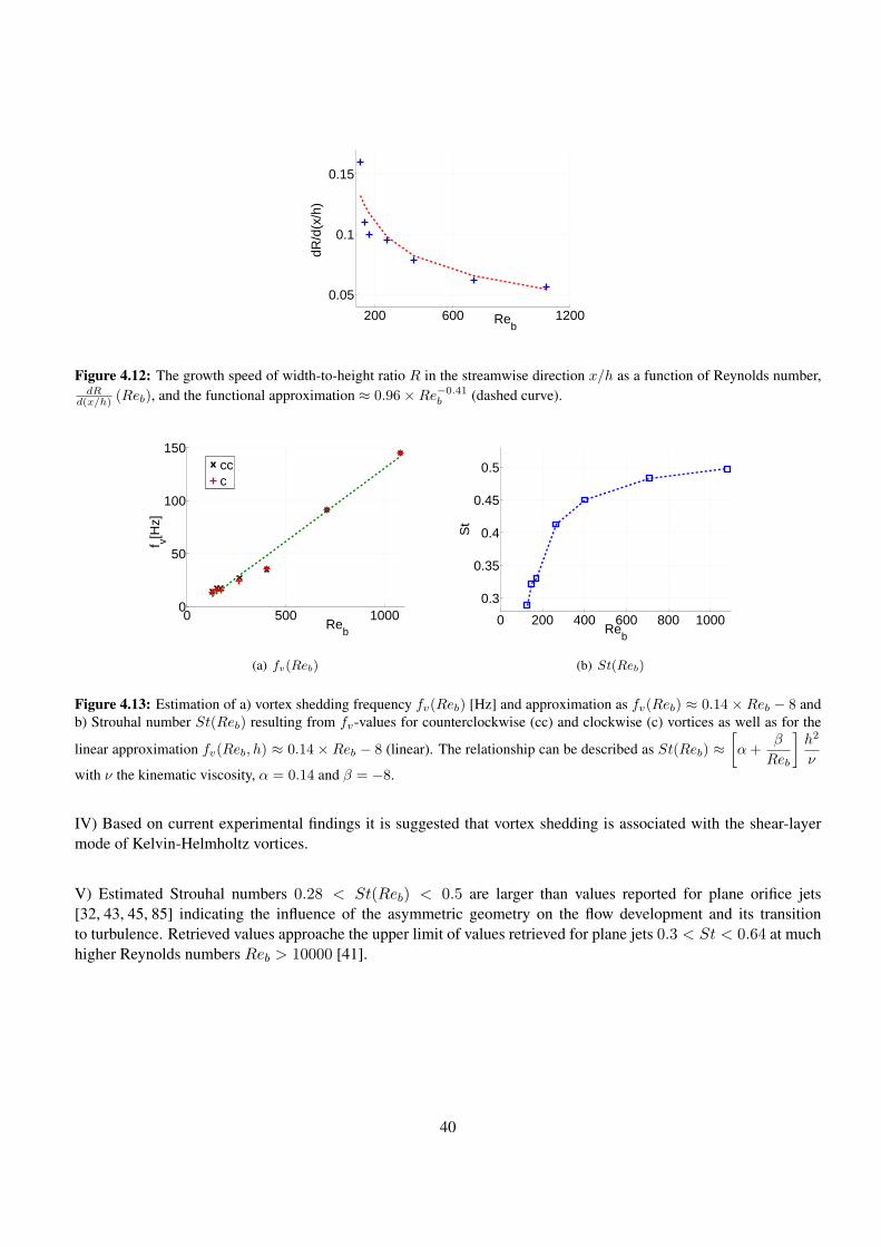
200 600 1200

0.05

0.1

0.15

Reb

dR/d

(x/h

)

Figure 4.12: The growth speed of width-to-height ratio R in the streamwise direction x/h as a function of Reynolds number,dR

d(x/h) (Reb), and the functional approximation ≈ 0.96×Re−0.41b (dashed curve).

0 500 10000

50

100

150

Reb

f v[Hz]

ccc

(a) fv(Reb)

0 200 400 600 800 1000

0.3

0.35

0.4

0.45

0.5

Reb

St

(b) St(Reb)

Figure 4.13: Estimation of a) vortex shedding frequency fv(Reb) [Hz] and approximation as fv(Reb) ≈ 0.14× Reb − 8 and

b) Strouhal number St(Reb) resulting from fv-values for counterclockwise (cc) and clockwise (c) vortices as well as for the

linear approximation fv(Reb, h) ≈ 0.14 × Reb − 8 (linear). The relationship can be described as St(Reb) ≈[

α+β

Reb

]

h2

νwith ν the kinematic viscosity, α = 0.14 and β = −8.

IV) Based on current experimental findings it is suggested that vortex shedding is associated with the shear-layer

mode of Kelvin-Helmholtz vortices.

V) Estimated Strouhal numbers 0.28 < St(Reb) < 0.5 are larger than values reported for plane orifice jets

[32, 43, 45, 85] indicating the influence of the asymmetric geometry on the flow development and its transition

to turbulence. Retrieved values approache the upper limit of values retrieved for plane jets 0.3 < St < 0.64 at much

higher Reynolds numbers Reb > 10000 [41].

40

Chapter 5

Validation of flow models

Some examples of validation of flow models are given.

5.1 Convergent axisymmetrical nozzle

Studies1 dealing with wind tunnel design are multiple illustrating the importance of the upstream geometry on the

flow characteristics at the inlet of a wind tunnel working section [8, 25, 51, 65, 69]. Besides, characterisation of the

exit profile of the nozzle, corresponding to the inlet portion to the working section, attention is given to avoid adverse

pressure gradients along the nozzle walls in order to favour low turbulence inflow to the working section.

Despite the amount of research available in aeronautics, inflow conditions are not or only marginally accounted for

when designing an experimental flow facility for experimental validation on a smaller scale. Nevertheless, a laminar

inflow with known boundary layer characteristics is of interest in order to limit the influence of upstream flow con-

ditions on downstream flow development and noise production.

Obviously, the sought laminar and known inflow conditions can be obtained by mounting a pipe upstream the replica

in order to ensure a fully developed Poiseuille flow. Nevertheless, for the aimed range of moderate Reynolds num-

bers the required pipe length results in a large experimental setup (orders of meters [50, 56, 117]) so that a smaller

setup is if not more practical at least more elegant. Consequently, it is chosen to study a short contraction geometry

of limited length (6cm) depicted in Fig. 3.6 and fully described by (3.3) with a geometrical scale adapted to applica-

tions favouring a small-sized nozzle.

In order to test the contraction experimentally, accurate transverse velocity profiles at the exit of the proposed axisym-

metrical contraction nozzle with contraction ratio CR = 21.8 and lenght 6cm are measured by hot-film anemometry

from which boundary layer characteristics can be derived [12,87,111]. As such the experimentally estimated bound-

ary layer characteristics provide data in order to validate laminar flow models since the turbulence level at the nozzle

centerline exit is less than 1% for all velocities.

1Main publications: [30, 39].

41

The flow through the nozzle is modelled with Thwaites axisymmetrical boundary layer solution [79,97,98] in order

to validate the dependence of the shape factor and skin friction parameter on the Thwaites parameter instead of rely-

ing on tabulated values reported in literature [9], since it is known that the dependence on Thwaites parameter varies

with the flow and geometrical conditions. Consequently, the sought experimental validation of Thwaites method is

two-fold in order to validate the measured flow characteristics at the nozzle exit as well as to consider the influence of

the dependence of the shape factor and skin friction parameter on Thwaites parameter for low to moderate Reynolds

numbers in the range 300 < Re < 20200.

The following observations are made:

I) It is observed on the measured exit velocity profiles that the variation in the mean velocity is lower than ±0.5%

for all assessed Re whereas the boundary layer grows rapidly for Re ≤ 3300. In addition, velocity measurements

in the boundary layer with high spatial accuracy (spatial step of 10µm) are performed to estimate the displacement

thickness δ1, momentum thickenss δ2 and shape factor H . Consequently, the proposed nozzle is of use for applica-

tions requiring low turbulence inflow and known boundary layer characteristics at the exit of a nozzle with limited

size as is the case for experimental validation of flow modelling.

II) Thwaites laminar axisymmetrical boundary layer solution using modified universal functions is applied to model

the flow through the nozzle. Two constants are introduced in the universal functions describing the skin friction

parameter and the shape parameter in order to account for the influence of flow and geometrical conditions. Com-

paring modelled and measured quantities at the nozzle exit shows that Thwaites solution provides good predictions

for Re > 3300, i.e. before the onset of boundary layer growth as shown in Fig. 5.1(a). Furthermore, in general

it is seen that in particular when boundary layer characteristics are of interest adding non-zero constants (denoted

cH,S 6= 0) to the universal functions increases the model accuracy in particular as the Re-number decreases.

3300 6600 9900 13200 16500 1980020

22

24

26

28

30

32

U2/U

1

Reb

D2=21.4, c

H,S≠0

D2=21.4, c

H,S=0

measured

ideal

(a)

3300 6600 9900 13200 16500 198000

0.5

1

1.5

2x 10−3

Reb

δ 1 [m]

measured 10µm

measured 100µmc

H,S ≠ 0

cH,S

= 0

(b)

Figure 5.1: a) Measured and modelled exit centerline velocity U2 normalised by the inlet centerline velocity of the nozzle U1

for a fixed contraction ratio of CR = 21.8 (dashed line) associated with an ideal fluid in a contraction. As a reference also the

measured centerline velocity is indicated. Modelled values are obtained for the additional coefficients set to zero (cH,S = 0) or

not (cH,S 6= 0). b) Comparison of modelled and measured displacement thickness δ1 at the exit of the nozzle with CR = 21.8.

As before additional coefficients are set to zero (cH,S = 0) or not (cH,S 6= 0).

42

5.2 Asymmetrical constriction

The2 pressure distribution along an rigid asymmetrical channel constriction depicted in Fig. 3.12 is predicted from

the upstream pressure and geometrical information. Several assumptions on the flow and the constriction geometry

are experimentally assessed. The model performance of corresponding flow models with increasing complexity is

systematically and quantitatively validated.

The following observations are made:

I) It is shown from a dimensionless analysis that, in first approximation, the fluid flow through the ‘in-vitro’ replica

can be described as steady and incompressible. Measured velocity profiles and measured pressures at different places

along the converging part of the constriction confirmed the relevance of a bidimensionnal flow description whereas

the viscous pressure losses can be neglected outside the boundary layer. Furthermore the velocity profiles reveal an

asymmetry of the flow downstream of the constriction due to the geometrical asymmetry illustrated in Fig. 5.2.

(a) (b) (c)

Figure 5.2: a) Measured vertical (y-axis) velocity profile at 9mm downstream the minimum constriction of 2.3mm. Note

the asymmetrical flow behaviour for φ = 100l/min. b) Measured bidimensional velocity profile illustrating jet formation

and flow separation along diverging part of replica for steady flow of φ = 40l/min and minimum aperture 3mm. A step of

1mm is applied in the longitudinal x-direction and 0.05mm in the transverse y-direction. c) Reduced Navier Stokes (RNSP)

computation (Reb = 500). The two uppper and lower boundary layers and the ideal fluid appear from the computation. The

interaction between the ideal fluid and the boundary layers is the core of the Interactive Boundary Layer theory [54].

II) Transversal pressure measurements on both sides of the constriction show that the influence of the asymmetry

on the measured pressure within the constriction is negligible. This point is further confirmed by considering the

predictions obtained by a two dimensional flow description from the boundary layer solution and Reduced Navier

Stokes simulations. The use of these two dimenstional flow descriptions result in a physical prediction of the position

of flow separation as illustrated in Fig. 5.3.

III) It is found that the outcome of a classical one dimensional flow description is sufficient in applications where

only prediction of the volume flow is strived, but fails to predict the pressure distribution as shown in Fig. 5.4. Quan-

titative experimental validation shows that both for the bulk velocity as for the pressure distribution two dimensional

flow descriptions yield pressure predictions within an accuracy of 15%. Application of the Reduced Navier Stokes

equations are slightly favored since they allow to account for the asymmetry in the geometry.

2Main publications: [54, 103, 110].

43

Figure 5.3: Predicted flow separation position.

(a) (b)

Figure 5.4: Influence of estimation of flow separation on predicted pressure distribution in case of one dimensional flow de-

scription: a) example b) Error estimation with upstream p0 (dashed) or downstream pM (full) pressure at minimum constriction

as known input variable for ad hoc assumption c = 1.2.

5.3 Constriction shapes: fixed and movable

Simplified3 simplified quasi one-dimensional flow models and derived inverse models are validated for steady and

unsteady flow conditions for the constriction shapes depicted in Fig. 3.11. The aimed models are derived from the

irrotational one-dimensional flow equation corrected for viscous effects and flow unsteadiness. The inverse flow

models outcome against the direct model input. Next inverse flow models are validated on experimental data ob-

tained for different glottal constriction shapes and flow conditions. The inverse model performance is discussed with

respect to the accuracy of the direct model. More advanced models describing accounting for the existence of the

boundary layer are assessed.

The following observations are made:

I) Inverse models derived from quasi one-dimensional flow models are formulated in order to retrieve the main

3Main publications: [17, 19, 20].

44

physical variables and models parameters, i.e. the upstream pressure, the minimum constriction height or the flow

separation coefficient. The accuracy of the inverse models is validated firstly against theoretical simulations obtained

with the corresponding direct models and secondly against experimental data. The proposed inverse models allow

to retrieve the original direct model input exactly with a minimum of computational effort. Moreover the severe

influence of flow separation, wall viscosity and unsteadiness due to wall movement on the model predictions is

pointed out for respectively a divergent round constriction shape, small apertures within the order of magnitude of

the viscous steady boundary layer thickness and high Strouhal numbers. Experimental validation in both steady and

unsteady flow conditions is achieved on rigid replicas with uniform and round constriction shapes in order to study

the impact of respectively wall viscosity and flow separation on the inverse model perfomances. Some experimental

and model results are illustrated in Fig. 5.5.

(a) (b)

Figure 5.5: a) Measurements (points) and model predictions for the round vocal folds vibrating at 25Hz: (top) minimum

constriction height hg , (middle) upstream pressure p0 and (bottom) pressure at the minimum constriction height pg . Predictions

are computed with cs = 1.08 and given by the steady Bernoulli (thin dashed line), steady Poiseuille (thin solid line), unsteady

Bernoulli (thick solid line) and unsteady Poiseuille (thick dashed line) models. b) Smoke visualisation of the flow separation

within the round vocal fold replicas with the minimum constriction height hg = 1mm. The separation positions corresponding

to three modified Reynolds numbers, Reδ = Rehg/L with L the length of the constriction, are indicated.

II) It appears that both wall viscosity and the position of flow separation determine the accuracy of the inverse quasi

one-dimensional models. A mean prediction accuracy of 20% for the sought physical variables can be achieved for

a divergent round constriction shape in case of the inverse models account for wall viscosity and a suitable flow

separation coefficient is applied. Remark that the necessity of a corrective term related to viscosity outlines the

limitations of the one-dimensional inviscid Bernoulli model. Moreover the predictions errors of the models increase

whenever the contribution of the viscosity related term to the estimated quantities decreases. Next the performance

of the inverse models is seen to reflect the accuracy of the direct models. Therefore on one hand it seems interesting

to include the error sensitivity to input variables in the minimization problem and on the other hand the use of more

advanced flow models is motivated. A first intermediate step might be considered in order to validate the value of the

separation coefficient as a function of the Reynolds number from more advanced glottal flow models. Comparaison

of models with different complexity is shown in Fig. 5.6.

45

(a)

(b)

(c)

Figure 5.6: Ratio between the upstream pressure p0 and the pressure at the minimum constriction height pg obtained experi-

mentally and simulated a) for the uniform constriction and b) for the round constriction. c) Separation coefficient cs obtained

by inversion with one-dimensional model and simulated by Thwaites and laminar two-dimensional Navier Stokes for the round

constriction.

5.4 Rectangular nozzle with 1 gradual and 1 sharp obstacle

A4 rectangular nozzle with 1 gradual and 1 sharp obstacle is presented in Fig. 3.10 and reminded in Fig. 5.7. In

the following it is aimed to validate simple one-dimensional laminar flow models, assumed in Bernoullis equation,

corrected by several ‘ad-hoc’ corrections to describe the influence of vorticity and turbulence on the mean flow.

The gap between the upstream gradual and sharp obstacle (between 0 and 81% of the unconstricted channel height)

as well as the constriction degree at the sharp obstacle (between 0 and 96% of the unconstricted obstacle) are

4Main publications: [101, 109].

46

systematically varied. In addition, flow conditions are varied so that the range of Reynolds numbers is varied up

to Reb < 15000. The flow is characterized by measuring the volume flow rate and performing point pressure

measurements at different positions along the replica indicated in Fig. 3.10.

0 i1 si1 i2 si2 i3

x

h0

w

Figure 5.7: Schematic overview of the geometry: rectangular channel with fixed width w characterized by height variation

h(x). The unconstricted channel height is denoted h0 and two constrictions are inserted spanning the intervals ]i1 si1] and

]i2 si2]. The x-axis indicates the main flow direction.

The following observations are made:

I) Point pressure are measured at several streamwise locations and appeared to vary significantly over the range of

imposed geometrical gaps. In addition, varying the gap between the upstream gradual and sharp obstacle while

maintaining the aperture at the sharp obstacle is seen to influence the pressure at the sharp obstacle. Consequently,

besides the aperture at the sharp obstacle aperture, the length of the gap between both obstacles influences the result-

ing airflow. This is confirmed by fitting the measured pressure drop as function of imposed geometrical parameters

since the accuracy of the volume flow rate estimation increases with 40% when the length of the gap between both

obstacles is taken into account as well.

II) Measured pressures and volume airflow rates are compared to the outcome of one-dimensional flow models

assuming a laminar incompressible irrotational and one-dimensional flow governed by Bernoulli’s equation to which

corrections are applied for viscosity, sudden geometrical expansion, sudden geometrical constriction and bending. In

presence of the upstream gradual obstacle, the accuracy for each set of geometrical parameters expressed as a mean

error for all predicted quantities and all imposed upstream pressures yields < 30%. The relevance of additional

corrections (resulting in the smallest errors) varies as function of the assessed geometrical parameter set. For very

small (≤ 58%) or very large (≥ 96%) constriction degrees at the sharp obstacle, the most accurate model is obtained

by accounting for viscosity regardless the separation distance between both obstacles. For intermediate constriction

degrees, in the interval [58 96]%, narrowing the gap between both constrictions causes the most accurate model to

shift from constriction to bending. Therefore, the geometrical parameter corresponding to the gap length, although

not explicitly appearing as a parameter in the validated one-dimensional models, does determine the appropriate

corrective term for the applied cost function. In addition, it is interesting to note that the best model accuracy is

the lowest for constriction degrees at the sharp obstacle (≈ 60%) for which the influence of distance between both

obstacles on the measured pressures is most significant. The best model accuracy is shown in Fig. 5.8.

III) Consequently, one-dimensional flow models can be applied to describe the flow through the vocal tract when

accounting for the relevant corrections in order to compensate, on geometrical considerations, for the non realistic

assumption of a laminar and irrotational flow.

47

Figure 5.8: Overall best mean model error J(q, L1, h2) of the models q(L1, h2) with L1 denoting the gap length between both

obstacles and h2 the aperture at the sharp obstacle.

5.5 Rectangular nozzle with 1 sharp obstacle

Velocity5 data are provided downstream an sharp obstacle in a rectangular uniform channel as shown in Fig. 3.9. The

inflow is steady and the Re-number is set to Re = 4000. The obstruction degree yields 70% and the width-to-height

ratio is set to 4 to ensure two-dimensional flow. A comparison of experimental and numerical mean and turbulent

velocity data obtained by Large Eddy Simulation (LES) is provided in the near flow field downstream the obstacle

from x = 0 up to x/h = 1.5 where h denotes the aperture. Both the inner and outer layers of the jet issuing from

the aperture are sought. The characterisation is inspired on features commonly observed for plane wall jets since a

two-layer shear flow can be expected [23, 55, 100].

Experimental as well as numerical flow data for a two-dimensional jet issuing from a sharp constriction for a flow

with Reynolds number 4000. In particular the near field is studied since a good characterisation is needed in order

to describe sound production due to the interaction of an airflow with the obstacle.

The following observations are made:

I) A first comparison between simulated and experimental velocity features is obtained by quantifying features

typically dealt with in studies of a plane wall jet as illustrated in Fig. 5.9. This is motivated since the current problem

is basically thought of as a two-layer shear flow consisting of an inner layer (similar to a boundary layer) and an outer

layer (similar to a free shear layer) as is the case for a plane wall jet. Nevertheless, the current results, numerical as

well as experimental, show that the interaction between the two generic layers leads to a more complex near flow

field for which more layers can be distinguished. Therefore, future studies should consider the flow field in more

detail; i.e. involving both the near and the fully developed region in order to validate established self-similar models

and scaling laws for the plane wall jet.

5Main publications: [35, 37, 108].

48

(a) (b)

Figure 5.9: a) Schematic illustration of experimental setup and nozzle with SHF denoting stationary hot film (SHF) anemom-

etry. The main flow direction is indicated by a bold arrow. Initial data stations for transverse (y < 0.5mm and ∆y =0.1mm)

and longitudinal (x < 0.5mm ∆x = 0.1mm) profiles gathered downstream the trailing edge of the obstacle, corresponding

to x/h = 0 and y/h = 1, for SHF measurements (transverse +, longitudinal ◦) are indicated. In addition, transverse profiles

taken from simulations (×) for comparison are given as well. b) Nozzle and some major geometrical and flow parameters

derived from plane wall jet nomenclature [23]: transverse flow direction y, longitudinal flow component Ux(x) in the main

flow direction x indicated by a bold arrow, characteristic velocity at the constriction outlet U0 at x ≈ 0, aperture height h ,

channel height h0, ym(x) distance from the wall up to the position of maximum flow velocity Um(x) in the transversal velocity

profile, y1/2(x) distance from the wall up to the outer position where the velocity corresponds to Um/2(x).

II) From the comparison of the experimental and simulated flow features, illustrated in Fig. 5.10, it is seen that the

mean flow fields show the same general tendencies, but differ when considering the quantified features. The main

common observations for the mean velocity include: 1) the position of maximum velocity ym shifts towards the wall

for increasing downstream position, 2) the maximum mean velocity Um increases downstream the constriction, 3)

the jet width is seen to decrease for increasing downstream position, 4) as does the ratio of the position of maximum

velocity to the outer half width ym/y1/2. Nevertheless, some important differences are observed from the quantified

mean velocity features with respect to the structure of the jet: 1) the experimentally observed jet is broadened

compared to the numerical jet, 2) the experimental mean velocity exhibits a narrow peak for y/h ≈ 1, which is

absent for the simulated data, 3) the position of maximum velocity is reached for y/h ≈ 1 on the experimental data,

which is larger than for the simulated data and finally 4) the ratio of the position of maximum velocity to the outer

half width ym/y1/2 is close to one for the experimental data. The observed differences are the result of increased

mean velocity and mean velocity gradients in the vicinity of the teeth edge, i.e. y/h ≈ 1, for the experimental data

compared to the simulated data. Both observations are important considering vorticity. The narrow peak near the

obstacle edge, observed on the measured mean velocity profiles, is accompanied with a narrow symmetrical peak in

turbulence intensity up to 10%. The observed peak is absent in the simulated flow field, which is laminar in the near

field downstream the constriction. It should be noted that although more accurate measurements can be performed,

e.g. by using other measurement techniques, the observed differences largely exceed the uncertainty of the velocity

measurements and are therefore significant.

49

Figure 5.10: Measured (meas) and simulated (sim) near field evolution 0 < x/h < 1.5, for a) position of maximum velocity

and outer position of half the maximum velocity y1/2 ( simulated = × and measured = +) and ym (simulated = � and measured

= ⋄). b) ratio of maximum velocity to characteristic outlet velocity Um/U0. c) ratio of positions ym and y1/2, i.e. ym/y1/2.

50

Chapter 6

Applications to the upper airways

The geometries, flow models and flow characterisation dealt with in the previous chapters are relevant for applica-

tions to the upper airways. In the following three examples are given: phonation, fricative production and obstructive

sleep apnea.

6.1 Phonation

Phonation1 or human voiced speech production can be generally represented as a fluid-structure interaction between

the airflow coming from the lungs and the vocal folds tissues in the glottis for which a schematic representation is

depicted in Fig. 6.1. Consequently, besides a flow model, a mechanical and acoustic model is required as well.

acoustic modelfluid flow model

mechanical model

Figure 6.1: Schematic representation of the model approach for speech production.

6.1.1 Theoretical model and stability analysis

The theoretical symmetrical two-mass model is schematically depicted in Fig. 6.2. In the following the model

detailed in [61,83] is briefly outlined and the parameter γ is introduced. Next, the system equations resulting from a

1Main publications: [18, 60, 62, 83, 104].

51

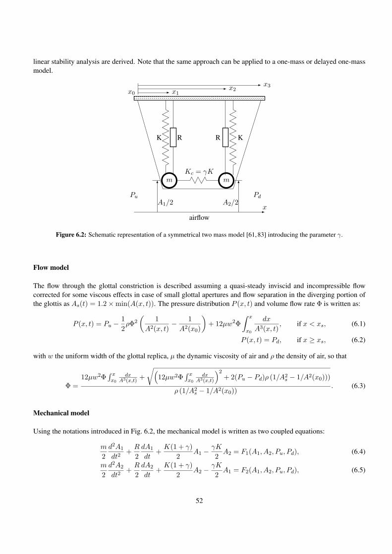
linear stability analysis are derived. Note that the same approach can be applied to a one-mass or delayed one-mass

model.

x0 x1x2

x3

airflow

Pu Pd

x

K R

m

KR

mKc = γK

A2/2A1/2

Figure 6.2: Schematic representation of a symmetrical two mass model [61, 83] introducing the parameter γ.

Flow model

The flow through the glottal constriction is described assuming a quasi-steady inviscid and incompressible flow

corrected for some viscous effects in case of small glottal apertures and flow separation in the diverging portion of

the glottis as As(t) = 1.2×min(A(x, t)). The pressure distribution P (x, t) and volume flow rate Φ is written as:

P (x, t) = Pu − 1

2ρΦ2

(

1

A2(x, t)− 1

A2(x0)

)

+ 12µw2Φ

∫ x

x0

dx

A3(x, t), if x < xs, (6.1)

P (x, t) = Pd, if x ≥ xs, (6.2)

with w the uniform width of the glottal replica, µ the dynamic viscosity of air and ρ the density of air, so that

Φ =12µw2Φ

∫ xx0

dxA3(x,t)

+

√

(

12µw2Φ∫ xx0

dxA3(x,t)

)2+ 2(Pu − Pd)ρ (1/A2

s − 1/A2(x0)))

ρ (1/A2s − 1/A2(x0))

. (6.3)

Mechanical model

Using the notations introduced in Fig. 6.2, the mechanical model is written as two coupled equations:

m

2

d2A1

dt2+R

2

dA1

dt+K(1 + γ)

2A1 −

γK

2A2 = F1(A1, A2, Pu, Pd), (6.4)

m

2

d2A2

dt2+R

2

dA2

dt+K(1 + γ)

2A2 −

γK

2A1 = F2(A1, A2, Pu, Pd), (6.5)

52

with F1,2 the force exerted by the fluid on the first and second mass respectively. The mechanical equations at

equilibrium reduces to:

K(1 + γ)

2A1 −

γK

2A2 = F1(A1, A2, Pu, Pd = 0), (6.6)

K(1 + γ)

2A2 −

γK

2A1 = F2(A1, A2, Pu, Pd = 0), (6.7)

from which the equilibrium positions for a given upstream pressure Pu are derived by a fixed point method.

Assuming a small perturbation (a1, a2, pu, pd) of the quantities around the equilibrium values eq = (A1, A2, Pu, Pd =0) as:

A1 = A1 + a1, A2 = A2 + a2, (6.8)

Pu = Pu + pu, Pd = Pd + pd, (6.9)

results in the following set of equations:

m

2

d2a1dt2

+R

2

da1dt

+K(1 + γ)

2a1 −

γK

2a2 =

∂F1

∂A1

∣

∣

∣

∣

∣

eq

a1 +∂F1

∂A2

∣

∣

∣

∣

∣

eq

a2 +∂F1

∂Pu

∣

∣

∣

∣

∣

eq

pu +∂F1

∂Pd

∣

∣

∣

∣

∣

eq

pd, (6.10)

m

2

d2a2dt2

+R

2

da2dt

+K(1 + γ)

2a2 −

γK

2a1 =

∂F2

∂A1

∣

∣

∣

∣

∣

eq

a1 +∂F2

∂A2

∣

∣

∣

∣

∣

eq

a2 +∂F2

∂Pu

∣

∣

∣

∣

∣

eq

pu +∂F2

∂Pd

∣

∣

∣

∣

∣

eq

pd. (6.11)

Acoustic model

The acoustic set of equations is given as:

d2ψd

d2t+ωd

Qd

dψd

dt+ ω2

dψd =Zdωd

Qdφ, (6.12)

d2ψu

d2t+ωu

Qd

dψu

dt+ ω2

uψu = −Zuωu

Quφ, (6.13)

with ∂ψu,d/∂t = pu,d the acoustic pressure and φ the unsteady portion of the volume flow velocity downstream the

vocal folds, ωu,d the acoustical resonance pulsation, Qu,d the quality factor and Zu,d the peak value of the acoustical

impedance. As for the mechanical equations assuming small variations around equilibrium results in:

d2ψd

d2t+ωd

Qd

dψd

dt+ ω2

dψd =Zdωd

Qd

∂Φ

∂A1

∣

∣

∣

∣

∣

eq

a1 +∂Φ

∂A2

∣

∣

∣

∣

∣

eq

a2 +∂Φ

∂Pu

∣

∣

∣

∣

∣

eq

pu +∂Φ

∂Pd

∣

∣

∣

∣

∣

eq

pd

, (6.14)

d2ψu

d2t+ωu

Qd

dψu

dt+ ω2

uψu = −Zuωu

Qu

∂Φ

∂A1

∣

∣

∣

∣

∣

eq

a1 +∂Φ

∂A2

∣

∣

∣

∣

∣

eq

a2 +∂Φ

∂Pu

∣

∣

∣

∣

∣

eq

pu +∂Φ

∂Pd

∣

∣

∣

∣

∣

eq

pd

. (6.15)

53

Linear stability analysis

Consequently, assuming small variations around equilibrium results in a coupled set of equations obtained from (6.10), (6.11), (6.14) and (6.15):

md2a1dt2

+Rda1dt

− 2∂F1

∂Pu

∣

∣

∣

∣

∣

eq

dψu

dt− 2

∂F1

∂Pd

∣

∣

∣

∣

∣

eq

dψd

dt+

K(1 + γ)− 2∂F1

∂A1

∣

∣

∣

∣

∣

eq

a1 −

γK + 2∂F1

∂A2

∣

∣

∣

∣

∣

eq

a2 = 0, (6.16)

md2a2dt2

+Rda2dt

− 2∂F2

∂Pu

∣

∣

∣

∣

∣

eq

dψu

dt− 2

∂F2

∂Pd

∣

∣

∣

∣

∣

eq

dψd

dt−

γK + 2∂F2

∂A1

∣

∣

∣

∣

∣

eq

a1 +

K(1 + γ)− 2∂F2

∂A2

∣

∣

∣

∣

∣

eq

a2 = 0, (6.17)

d2ψd

d2t− Zdωd

Qd

∂Φ

∂Pu

∣

∣

∣

∣

∣

eq

dψu

dt+

ωd

Qd− Zdωd

Qd

∂Φ

∂Pd

∣

∣

∣

∣

∣

eq

dψd

dt− Zdωd

Qd

∂Φ

∂A1

∣

∣

∣

∣

∣

eq

a1 −Zdωd

Qd

∂Φ

∂A2

∣

∣

∣

∣

∣

eq

a2 + ω2dψd = 0, (6.18)

d2ψu

d2t+

ωu

Qd+Zuωu

Qu

∂Φ

∂Pu

∣

∣

∣

∣

∣

eq

dψu

dt+Zuωu

Qu

∂Φ

∂Pd

∣

∣

∣

∣

∣

eq

dψd

dt+Zuωu

Qu

∂Φ

∂A1

∣

∣

∣

∣

∣

eq

a1 +Zuωu

Qu

∂Φ

∂A2

∣

∣

∣

∣

∣

eq

a2 + ω2uψu = 0. (6.19)

The system can be expressed in state-space form as

X =MX (6.20)

with X = [a1, a2, ψu, ψd, da1/dt, da2/dt, dψu/dt, dψd/dt] and M defined as:

M =

0 0 0 0 1 0 0 00 0 0 0 0 1 0 00 0 0 0 0 0 1 00 0 0 0 0 0 0 1

−K(1+γ)−2

∂F1

dA1|eq

m

γK+2∂F1

dA2|eq

m 0 0 −Rm 0 2

m∂F1

∂Pu|eq 2

m∂F1

∂Pd|eq

γK+2∂F2

dA1|eq

m −K(1+γ)−2

∂F2

dA2|eq

m 0 0 0 −Rm

2m

∂F2

∂Pu|eq 2

m∂F2

∂Pd|eq

Zdωd

Qd

∂Φ∂A1

∣

∣

∣

∣

∣

eq

Zdωd

Qd

∂Φ∂A2

∣

∣

∣

∣

∣

eq

0 −ω2d 0 0 Zdωd

Qd

∂Φ∂Pu

∣

∣

∣

∣

∣

eq

−

ωd

Qd− Zdωd

Qd

∂Φ∂Pd

∣

∣

∣

∣

∣

eq

−Zuωu

Qu

∂Φ∂A1

∣

∣

∣

∣

∣

eq

−Zuωu

Qu

∂Φ∂A2

∣

∣

∣

∣

∣

eq

−ω2u 0 0 0 −

ωu

Qd+ Zuωu

Qu

∂Φ∂Pu

∣

∣

∣

∣

∣

eq

−Zuωu

Qu

∂Φ∂Pd

∣

∣

∣

∣

∣

eq

. (6.21)

54

For a known set of initial conditions the system will become instable, corresponding to oscillation onset, in case the

real portion of an eigenvalue of M is positive. The corresponding oscillation pulsation is obtained as the imaginary

portion of the eigenvalue.

Note that in the foregoing collision is detected following the criterion hc = A/w < hcrit in which case the values

of K and R are increased to K = 4K and R = R+ 2√Km. The fixed collision threshold hcrit is set to 0.02 mm.

6.1.2 Example of results

The symmetrical deformable constriction depicted in Fig. 3.16 is used to validate theoretical low-dimensional mod-

els. Experimental results establish the influence of independent initial conditions on the observed oscillation onset

and offset pressures as well as the oscillation frequency. In a first attempt to include the measured open area in the

modelling, commonly used low order models are assessed for which the geometrical input parameter is derived on

the measured open area as an averaged aperture. Comparison of measured and modelled onset and offset upstream

pressure threshold for auto-oscillation is shown in Fig. 6.3.

(a) (b) (c)

Figure 6.3: Experimentally observed onset (×), offset (◦) a) modelled Pthres for separator 0.0 and b) modelled Pthres 1.0 mm

and c) modelled F0: (+) two-mass model with hcrit = 0.02 mm and geometrical h0a mass estimation, (⊳) two-mass model with

hcrit = 0.5 mm and geometrical h0a mass estimation, (�) one-mass model with hcrit = 0.02 mm and geometrical h0a mass

estimation, (♦) two-mass model with hcrit = 0.02 mm and mass estimated from the mechanical resonance frequency.

It is seen that the models are capable of predicting the oscillation thresholds and frequencies qualitatively. Quanti-

tative predictions remain difficult for mainly three reasons: 1) the estimation of the model parameter m is critical,

2) the model itself does not accurately describe some crucial phenomena like the contact of the lips or of the vocal

folds and 3) an averaged aperture does not take account of the influence of viscosity in case of partial closure of the

open area. The influence of the collision model is illustrated in Fig. 6.4.

6.2 Voiceless sound production: fricatives

Research aiming physical modelling of human speech production is mainly concentrated on voiced sound produc-

tion. Aerodynamic and aeroacoustic principles have been introduced in speech production studies dealing with

fricatives since [26]. This pioneering work has been further developed by experimental as well as modeling stud-

ies: [4,44,52,90–92]. As a result, the underlying mechanism of fricative sound production is generally described as

55

Figure 6.4: Influence of the aperture criterion hcrit triggering the application of the collision model on the simulated Pthres for

features derived from ha (�) and hc (◦) for separator 0.5 mm and Pin=11000 Pa. The dashed line indicates the experimentally

observed Pthres value.

noise produced due to the interaction of a turbulent jet, issued from a constriction somewhere in the vocal tract, with

a downstream wall or obstacle. Consequently, the position and shape of articulators like tongue and teeth determine

the generation and development of the jet as well as its downstream interaction with a wall or obstacle as is indeed ob-

served on human speakers [70,81]. It follows that experimental and simulation studies have been performed in order

to characterize and quantify the influence of articulators position and shape on the sound produced [72, 77, 89, 90].

Nevertheless, the previous focus on the acoustics of fricative noise production and not on the flow. Therefore, a

necessary step to describe unvoiced fricative sound production is to characterise the flow through the vocal tract

downstream the glottis, an extensive and systematic validation of flow through the vocal tract downstream the glottis

for configurations relevant for unvoiced sound production is lacking as recently pointed out [10, 44]. Therefore, in

order to gain insight in the flow development it is necessary 1) to perform a systematic comparison of measurements

on simplified mechanical vocal tract models to physical flow models and 2) to gradually increase the complexity of

the flow models.

The design of the nozzles outlined in the previous chapters fulfill these requirements so that at term the described

characterisation and model validation is likely to contribute to physical modelling and related applications of human

fricative speech sound production since:

• Extended axisymmetrical nozzles: relatively short extended convergent-divergent diffusers with length-to-

diameter ratios Lt/d < 20 are considered [74]. Such geometrical configurations, although a crude approxima-

tion, are relevant to flow through the human upper airways since: 1) a narrowed upstream passage is present

in the upper airways, e.g. at the larynx (glottis) and the lips, or naturally created in the oropharynx during

articulation [28, 44, 64, 95] and 2) a typical vocal tract length for a newborn and adult is 7 and 18cm respec-

tively [28,64,95]. Further variation of the geometrical length scale Lt, corresponding to varying the extension

length is e.g. due to morphology, pathology or articulation during speech production. Since the assessed flow

and geometries cover the range relevant to upper airway flow during speech production, initial conditions and

in particular initial turbulence levels at the exit of the sought extended nozzles are likely to exhibit important

variations depending on the articulator’s positions.

• Rectangular nozzle with 1 sharp obstacle: the position and geometry of the sharp obstacle matches the

physiological data of an upper incisor. As such the nozzle represents a single upper incisor inserted in a

channel and allows to study the flow around a teeth-shape obstacle.

56

• Rectangular nozzle with 1 gradual and 1 sharp obstacle: the current nozzle accounts for jet formation

upstream a sharp obstacle representing the tongue and teeth articulators. As such the flow data observed and

modelled for this nozzle geometry is mostly related to real life fricative production. Moreover observed sound

spectra do allow to reproduce typical spectra associated with human fricative production.

6.3 Obstructive sleep apnea

Obstructive2 sleep apnea can be generally represented as a fluid-structure interaction between the airflow coming

from the lungs and the upper airway tissues for which a schematic representation is depicted in Fig. 6.5. Conse-

quently, a flow and mechanical model are required to account for OSA.

fluid flow model

mechanical model

Figure 6.5: Schematic representation of the model approach for obstructive sleep apnea.

Experimental and modelled resuls on the asymmetrical deformable replica presented in Fig. 3.13 are compared in

Fig 6.6. The experimental results correspond to a collapse of about 25 % corresponding to the ‘in-vitro’ repro-

duction of a hypopnea syndrome due to the negative pressure forces along the constriction. In absence of flow the

minimum constriction coincides with the position of the pressure tap p1 at the centre of half cylinder. Increasing

the upstream pressure p0 results in negative pressures at all pressure taps, i.e. at the support centre 0, 8 and 16 mm

further downstream. Further increasing the pressure results in a further decrease 16 mm after the centre while at the

centre a positive pressure is retrieved. Therefore the curves confirm the displacement of the minimum constriction

in the flow direction prevailed in the dye experiment illustrated in Figure 3.15.

The overall model prediction agrees well with the experimental data. In all cases the error remains well below 20 %

considered as the upper limit for worst case error. Replica reopening is observed in Fig. 6.6(b) for experimental data

1. This behaviour can not be predicted by the applied model due to the assumption of quasi-steadiness. Reopening

is associated with the onset of instabilities retrieved in e.g. snoring. The flow limitation due to the wall displacement

characterising the collapse is for the examples showed in Figure 6.6 yield 49.9 and 69.6 %, respectively. The

percentages of flow limitation are comparable to ‘in-vivo’ order of magnitudes of about 50 % in case of hypopnea.

So both the theoretical as the experimental model are suitable to study at partial collapse and in particular the

presented experimental model is therefore a valuable alternative to the classical Starling resistor experiment. The

theoretical model is not capable to predict total collapse since among others a collision model is not taken into

account. The contact during the collision influences e.g. the onset of instabilities to a large extent.

2Main publications: [15, 16, 17, 103].

57

(a) ∆P=200Pa, Pin=200Pa

(b) ∆P=200Pa, h0

c=1.2mm, Pin=200Pa

(c) ∆P=290Pa, h0

c=0.87mm, Pin=400Pa

Figure 6.6: a) Measured pressures P(t) for the deformable replica Pa for the upstream pressure (p0) and for the pressure taps at

the positions indicated in Fig. 6.6 at the middle of the metal cylinder 0 (◦), 8 (△) and 16 (+) mm downstream. b,c) Simulation

of a hypopnea illustrating measured (+,◦,∗) and predicted (full line) centre height hc as a function of upstream pressure.

58

Chapter 7

Conclusion and perspectives

7.1 Conclusion

The current document reports on the study of moderate Reynolds number flow in a range 100 − 104 relevant to

phenomena associated with the human upper airways. Besides practical relevance the range of Reynolds numbers

is less studied in literature so that flow data are missing. In addition, since the human upper airways geometry

is very different from typical well designed nozzle geometries mostly dealt with in literature, the study of flow

through a-typical nozzles is needed. Since in particular in speech production most research deals with phonation the

study of nozzles suitable to mimic the e.g. the oral tract articulators are limited. The current document therefore

aims to contribute to the study of moderate Reynolds number flow through a-typical nozzles. Nevertheless, it is in no

way aimed to study flow through real human upper airway geometries. Instead some severe simplifications are made.

Different aspects of moderate Reynolds number flow are dealt with:

7.1.1 Experiments

From an experimental point of view a contribution is made to the development of experimental setups for flow mea-

surement and flow visualisation as well as aeroacoustic measurements. As such a simple setup and algorithm for hot

film/wire calibration in the range of low and moderate flow velocities is presented in order to obtain quantitative in-

formation of the velocity field at a given position. In addition to quantitative point measure by anemometry, a simple

setup for flow visualisation is used enabling a qualitative overall view of the flow field. Next, a setup for acoustic

measurements is realised aiming firstly to isolate from external noises due to either the flow facility, colleagues or

outdoor noises and secondly aiming to provide an approximation of free field conditions for sound registration.

Several simplified rigid mechanical replicas are presented starting from a tube or channel and gradually increasing

the complexity of the replica under study by introducing 1 or 2 obstacles with a sharp or more gradual constriction.

Consequently the presented mechanical replicas allow to study the flow at the exit of axisymmetrical tubes or two

dimensional channels for which among others the inlet geometry can be varied, the length of the carrier tube or

channel, the shape of the obstacle and the length of the constricted region. A step motor can be mounted to some of

the rigid obstacles so that the influence of wall movement on the flow can be studied.

59

In addition to rigid obstacles, two deformable replicas are outlined for which the initial aperture can be varied by

adding shims. As such, the replicas are in particular suitable to study the influence of initial conditions on the flow-

structure interaction.

7.1.2 Characterisation of jet development

Jet development at the exit of the axisymmetrical tubes and two-dimensional channels are characterised from hot-

wire anemometry and smoke visualisation. Transverse and longitudinal velocity profiles are quantified in order to

characterise main statistical features of the mean and fluctuating flow field. As such a start is made to take into

account turbulent flow in relation to simplified mechanical replicas of limited dimension and volume flow rate. In

addition, the coherent structures associated with the onset to turbulence are visualised and characterised by means

of simple image processing techniques.

In case of axisymmetrical tubes in particular the influence of the inlet geometry and tube extension length on the

measured velocity profiles is sought for different Reynolds numbers. Both the mean and turbulence level of the initial

profile at the tube outlet is observed to depend on both the Reynolds number as the tube extension length for fixed

diameter. From the longitudinal centerline velocity profiles the mean velocity decay is characterised by parameters

well studied in literature such as the decay constant, virtual origin and potential core length. It is observed that values

for Reynolds numbers approximating 1.1 × 104 correspond to values reported in literature for the decay constant

and potential core length although not for the virtual origin. In addition, the experimentally measured jet spreading

rate is used to estimate the turbulence viscosity. Smoke visualisation mainly confirms the hot-wire measurements

and makes their interpretation easier.

Vortex dynamics in the near field downstream an asymmetrical rectangular nozzle is studied in the range 100 <Re < 1100 based on rectangular vortex dynamics extracted from smoke visualisation images. As for the axisymmet-

rical nozzles the influence of the bulk Reynolds number on the spatial and temporal evolution of counterclockwise

and clockwise vortices is assessed. Vortex streamwise stretching is observed to decrease with Reynolds number and

the shedding frequency is seen to increase linearly with Reynolds number from which the Strouhal number can be

estimated.

7.1.3 Validation of flow models

Different flow models with increasing complexity are validated on experimental data mainly resulting from point

pressure measurements and hot wire anemometry.

Simplified direct and inverse one-dimensional flow models are seen to qualitative model the flow behaviour for two-

dimensional constrictions of different geometries. Nevertheless, the position of flow separation remains a crucial

aspect and an unphysical position is needed for an accurate description of the pressure distribution. Boundary layer

solutions are seen to strongly improve this drawback of one-dimensional flow modeling. Nevertheless, it is obvious

that the laminar flow models does not account for turbulence development and as such their use is limited down-

stream a constriction for which turbulence develops in the shear layers.

60

The performance of adding loss terms to one-dimensional laminar flow models based on geometrical considerations

in order to predict the mean flow in a channel with 2 obstacles is seen to result in a qualitative prediction. Neverthe-

less more complex models accounting for turbulence are required in order to increase the accuracy and to estimate

the fluctuating portion of the flow field. A start is made by simulating the flow through a two-dimensional channel

with one obstacle by large eddy simulation. Although a good qualitative agreement is obtained between the simu-

lated and measured flow field in the near field downstream the obstacle the quantitative dismatch remains.

7.1.4 Application to the upper airways

The previous described research is applied to phenomena associated with the upper airways such as speech produc-

tion and Obstructive Sleep Apnea (OSA).

At first application to a linear stability analysis of phonation is presented using the one-dimensional flow models.

Particular attention is given to the influence of mechanical model parameters and their relationship with experimen-

tally measurable quantities. Next, since turbulence is taken into account at term the current research is likely to

contribute to human fricative production.

Finally, an application is presented to obstructive sleep apnea.

7.2 Perspectives

Perspectives of the presented research are many.

It is obvious that despite the multitude of studied nozzle geometries and mechanical replicas it concerns mostly

axisymmetrical or two-dimensional nozzles so that it is of obvious interest to vary the geometry. Moreover most

of presented research deals with rigid nozzle geometries which does not account for a viscous layer adjactant to

the wall. Obviously the presence of such a layer influences the boundary layer development and an extension to

two-phase fluid is in particular interesting for pathological applications such as asthma.

It is aimed to apply the estimated turbulence viscosity in a simple turbulent flow model at least in order to predict

the flow along the centerline. Moreover the current experimental data need to be studied from the point of view of

flow stability in order to extent modeling of the flow. Besides an estimation of the fluctuating properties of the flow,

the next step is obvious aero-acoustic modeling in order to estimate the sound production as well as to consider the

influence of acoustics on the flow development and vice-versa.

Finally, although a great effort is made with respect to the development of the experimental setup, increasing the

measurement accuracy requires further development. It is aimed to obtain quantitative velocity information from

Particle Image Velocimetry. In addition, it is aimed to extent the anemometry measurements to more than one ve-

locity component. Moreover mostly steady flow is studied. Obviously the experimental setup needs to be developed

in order to account for unsteady flow. From the point of view of acoustic measurements it is of interest to consider

61

microphone antennes in order firstly to obtain information on the directivity and secondly on the source region.

Furthermore, mainly flow modelling is discussed although more complex mechanical modeling is needed in order

to describe complex fluid-structure interaction phenomena such as phonation, osa or lung sounds.

62

Bibliography

[1] Elastomeres datasheet, 2010.

[2] P. 0’Neill, J. Soria, and D. Honnery. The stability of low reynolds number round jets. Exp, 36:473–483, 2004.

[3] A. Abdel-Rahman, S. Al-Fahed, and W. Chakroun. The near-field characteristics of circular jets at low

Reynolds numbers. Mechanics Research Communications, 23:313–324, 1996.

[4] S. Adachi and K. Honda. CFD approach to fricative sound sources. In Proc. 6th International Seminar on

Speech Production, pages 1–4, Sydney, Australia, 2003.

[5] Inc ADINA R&D. A.D.I.N.A. Theory and Modeling Guide Volume III: ADINA CFD & FSI. Inc, Watertown,

MA, U.S.A., 2006.

[6] R. Antonia and Q. Zhao. Effect of initial conditions on a circular jet. Exp. Fluids, 31:319–323, 2001.

[7] G.K. Batchelor. An introduction to fluid dynamics. Cambridge Mathematical Library, 2000.

[8] J.H. Bell and R.D. Mehta. Contraction design for small low-speed wind tunnels. NASA STI/Recon Technical

Report N, 89:22, 1988.

[9] R.D. Blevins. Applied Fluid Dynamics Handbook. Krieger publishing company, Malabar, 1992.

[10] D. Bodony. The prediction and understanding of jet noise. Center for Turbulence Research Annual Research

Briefs, pages 367–377, 2005.

[11] B. Boersma, G. Brethouwer, and F. Nieuwstadt. A numerical investigation on the effect of the inflow condi-

tions on the self-similar region of a round jet. Phys. Fluids, 10:899–909, 1998.

[12] H.H. Bruun. Hot-wire anemometry. Oxford Science Publications, New York, 1995.

[13] P. Burattini, R. Antonia, S. Rajagopalan, and M. Stephens. Effect of initial conditions on the near-field

development of a round jet. Exp. Fluids, 37:56–64, 2004.

[14] T. Cebeci and J. Cousteix. Modeling and computation of boundary-layer flows. Springer, 2005.

[15] F. Chouly. Modelisation physique des voies aeriennes superieures pour le syndrome d’apnees obstructives du

sommeil. PhD thesis, 2005.

[16] F. Chouly, A. Van Hirtum, P.Y. Lagree, X. Pelorson, and Y. Payan. Modelling the human pharyngeal air-

way: validation of numerical simulations using in-vitro experiments. Medical & Biological Engineering &

Computing, 47:49–58, 2009.

[17] J. Cisonni. Modelisation et inversion d’un systeme complexe de production de signaux acoustiques: applica-

tion a la voix et aux pathologies. PhD thesis, Grenoble, France, 2008.

63

[18] J. Cisonni, A. Van Hirtum, X. Pelorson, and J. Lucero. The influence of geometrical and mechanical input

parameters on theoretical models of phonation. Acta Acustica, 2:291–302, 2011.

[19] J. Cisonni, A. Van Hirtum, X. Pelorson, and J. Willems. Theoretical simulation and experimental validation

of inverse quasi one-dimensional steady and unsteady glottal flow models. J. Acoust. Soc. Am., 124:535–545,

2008.

[20] J. Cisonni, A. Van Hirtum, Luo X.Y., and X. Pelorson. Experimental validation of quasi one-dimensional and

two-dimensional steady glottal flow models. Med. Biol. Eng. Comput., 48:903–910, 2010.

[21] R.C. Deo, J. Mi, and G.J. Nathan. The influence of Reynolds number on a plane jet. Physics of Fluids, 20,

2008.

[22] M. Deverge, X. Pelorson, C. Vilain, P. Lagree, F. Chentouf, J. Willems, and A. Hirschberg. Influence of

collision on the flow through in-vitro rigid models of the vocal folds. J. Acoust. Soc. Am., 114(6):1–9, 2003.

[23] J. Eriksson, R. Karlsson, and J. Person. An experimental study of a two-dimensional plane turbulent wall jet.

Experiments in Fluids, 20:50–60, 1998.

[24] O. Estienne. Etude aeraulique et aeroacoustique de la production de consonnes fricatives par modele

physique. PhD thesis, Grenoble University, 2010.

[25] F. Fang. A design method for contractions with square end sections. J. Fluid Eng., 119:454–458, 1997.

[26] G. Fant. The acoustic theory of speech production. Mouton, The Hague, 1960. p.328.

[27] H. Fellouah, C.G. Ball, and A. Pollard. Reynolds number effects within the development region of a turbulent

round free jet. International Journal of Heat and Mass Transfer, 52:3943–3954, 2009.

[28] W. Fitch and J. Giedd. Morphology and development of the human vocal tract: A study using magnetic

resonance imaging. J. Acoust. Soc. Am., 106:1511–1522, 1999.

[29] Y. Fujiso and A. Van Hirtum. Evaluation des performances d’une chambre d’isolation acoustique destinee a

la validation experimentale de production de parole. In Proc. RJCP, page 4, Grenoble, France, 2011.

[30] Y. Fujiso, B. Wu, X. Grandchamp, and A. Van Hirtum. Caracterisation d’un convergent axisymetrique. In

Proc. 20ieme CFM, page 6 (Accepted), Besancon, France, 2011.

[31] W. George. The decay of homogeneous isotropic turbulence. Phys. Fluids A, 4:1492–1509, 1992.

[32] W.K. George. Recent advances in Turbulence, chapter The self-preservation of turbulent flows and its relation

to initial conditions and coherent structures, pages 39–73. Hemisphere, New York, 1989.

[33] W.K. George, H. Abrahamsson, J. Eriksson, R.I. Karlsson, L. Lofdahl, and M. Wosnik. A similarity theory

for the turbulent plane wall jet without external streaming. J. Fluid Mech., 425:367–411, 2000.

[34] M. Germano, U. Piomelli, P. Moin, and W. Cabot. A dynamic subgrid-scale eddy viscosity model. Phys

Fluids A, 3:1760–1765, 1991.

[35] X. Grandchamp. Modelisation physique des ecoulements turbulents appliquees aux voies aeriennes

superieures chez l’humain. PhD thesis, Grenoble Universities, 2009.

[36] X. Grandchamp, Y. Fujiso, and A. Van Hirtum. Jet rond en aval d’une contraction brusque. In Proc. 20ieme

CFM, page 6 (Accepted), Besancon, France, 2011.

64

[37] X. Grandchamp, A. Van Hirtum, K. Nozaki, J. Cisonni, X. Pelorson, and S. Shimojo. Visualisation of moder-

ate reynolds number flow through a tooth-shaped nozzle. In Proc. 20th Int. Conf. of Acoustics (ICA), page 6,

Sydney, Australia, 2010.

[38] X. Grandchamp, A. Van Hirtum, and X. Pelorson. Experimental validation of simplified free jet turbulence

models applied to the vocal tract. In Proc. Int. Conf. on Acoustics (ICA), page 6, Madrid, Spain, September

2007.

[39] X. Grandchamp, A. Van Hirtum, and X. Pelorson. Hot film/wire calibration for low to moderate flow veloci-

ties. Meas. Sci. Technol., 21:115402, 2010.

[40] F.F. Grinstein. Vortex dynamics and entrainment in rectangular free jets. J. Fluids Mech., 437:69–101, 2001.

[41] E. Gutmark and C.M. Ho. Preferred modes and the spreading rates of jets. Phys. Fluids, 26:2932–2938, 1983.

[42] P.T. Harsha. Free turbulent mixing: a critical evaluation of theory and experiment. Technical report, 1971.

[43] C. Ho and P. Huerre. Perturbed free shear layers. Annu. Rev. Fluid Mech., 16:365–424, 1984.

[44] M.S. Howe and R.S. McGowan. Aeroacoustics of [s]. Proc. R. Soc. A, 461:1005–1028, 2005.

[45] F. Hsiao, Y. Lim, and J. Huang. On the near-field flow structure and mode behaviors for the right-angle and

sharp-edged orifice plane jet. Experimental Thermal and Fluid Science, In press:1–8, 2010.

[46] H.H. Hubbard, editor. Aeroacoustics of flight vehicles. Acoustical Society of America, 1995.

[47] A. Hussain and M. Zedan. Effects of the initial condition on the axisymmetric free shear layer: Effects of the

initial momentum thickness. Phys. Fluids, 20:1100–1112, 1978.

[48] H. Hussein, S. Capp, and W. George. Velocity measurements in a high Reynolds number momentum con-

serving axisymmetric turbulent jet. J. Fluid Mech., 258:31–75, 1994.

[49] S. Iio, K. Takahashi, Y. Haneda, and T. Ikeda. Flow visualisation of vortex structure in a pulsed rectangular

jet. J. of Visualization, 11:125–132, 2008.

[50] A. Johnstone, M. Uddin, and A. Pollard. Calibration of hot-wire probes using non-uniform mean velocity

profiles. Exp. Fluids, 39:1432–1114, 2005.

[51] N.L. Kachhara, P.L. Wilcox, and J.L. Livesey. A theoretical and experimental investigation of flow through

short axisymmetric contractions. In Proc. 5th Australian Conf. on Hydraulics and Fluid Mechanics, pages

82–89, Christchurch, New Zealand, 1974.

[52] M. Krane. Aeroacoustic production of low-frequency unvoiced speech sounds. J. Acoust. Soc. Am.,

118(1):410–427, 2005.

[53] S.J. Kwon and I.W. Seo. Reynolds number effects on the behavior of a non-buoyant round jet. Exp. Fluids,

38:801–812, 2005.

[54] P.Y. Lagree, A. Van Hirtum, and X. Pelorson. Asymmetrical effects in a 2D stenosis. European Journal of

Mechanics B/Fluids, 26:83–92, 2007.

[55] B.E. Launder and W. Rodi. The turbulent wall jet - measurements and modeling. Annu. Rev. Fluid Mech.,

15:429–459, 1983.

[56] T. Lee and R. Budwig. Two improved methods for low-speed hot-wire calibration. Meas. Sci. Technol.,

2:643–646, 1991.

65

[57] M. Lesieur, O. Metais, and P. Comte. Large-Eddy Simulations of Turbulence. Cambridge University Press,

New York, 2005.

[58] D. Lilly. A proposed modification of the Germano subgrid-scale closure method. Physics of Fluids, 4:633–

635, 1992.

[59] S.C. Ling and C.A. Wan. Decay of isotropic turbulence generated by a mechanically agitated grid. Phys.

Fluids, 15:1363, 1972.

[60] I. Lopez, A. Hirschberg, A. Van Hirtum, N. Ruty, and X. Pelorson. Physical modeling of buzzing artificial

lips: The effect of acoustical feedback. Acta Acustica, 92(6):1047–1059, 2006.

[61] N. Lous, G. Hofmans, N. Veldhuis, and A. Hirschberg. A symmetrical two-mass vocal-fold model coupled to

vocal tract and trachea, with application to prosthesis design. Acta Acustica, 84:1135–1150, 1998.

[62] J. Lucero, A. Van Hirtum, N. Ruty, J. Cisonni, and X. Pelorson. Validation of theoretical models of phonation

threshold pressure with data from a vocal fold mechanical replica. J. Acoust. Soc. Am., 125:632–635, 2009.

[63] T.G. Malmstrom, A.T. Kirkpatrick, B. Christensen, and K.D. Knappmiller. Centreline velocity decay mea-

surements in low-velocity axisymmetric jets. J. Fluid Mech., 246:363–377, 1997.

[64] R. McGowan. Perception of synthetic vowel exemplars of 4 year old children and estimation of their corre-

sponding vocal tract shapes. J. Acoust. Soc. Am., 120:2850–2858, 2006.

[65] R.D. Metha and P. Bradshaw. Design rules for small low speed wind tunnels. The Aeronautical J. of the Royal

Aeronautical Society, 18:443–449, 1979.

[66] J. Mi, R.C. Deo, and G.J. Nathan. Characterization of turbulent jets from high-aspect-ratio rectangular noz-

zles. Physics of Fluids, 17:4, 2005.

[67] J. Mi, P. Kalt, G. Nathan, and C. Wong. PIV measurements of a turbulent jet issuing from round sharp-edged

plate. Exp. Fluids, 42:625–637, 2007.

[68] J. Mi, D. Nobes, and G. Nathan. Influence of jet exit conditions on the passive scalar field of an axisymmetric

free jet. J. Fluid Mech., 432:91–125, 2001.

[69] T. Morel. Comprehensive design of axisymmetric wind tunnel contractions. J. Fluid Eng., 97:225–233, 1975.

[70] S. Narayanan, A. Alwan, and K. Haker. An articulatory study of fricative consonants using magnetic reso-

nance imaging. J. Acoust. Soc. Am., 98:1325–1347, 1995.

[71] H.B. Nottage. Report on ventilation jets in room air distribution. Technical report, Case Inst. of Technology,

Cleveland, Ohio, 1951.

[72] K. Nozaki, T. Akiyama, S. Shimojo, S. Maeda, and H. Tamagawa. Integration of computational fluid dynamics

and computational aero acoustics on grid for dental applications. In Proc.18th IEEE Symposium on Computer-

Based Medical Systems, pages 517–522, Ann Arbor, MI, USA, 2005.

[73] N. Panchapakesan and J. Lumley. Turbulence measurements in axisymmetric jets of air and helium. part 1.

air jet. J. Fluid Mech., 246:197–224, 1993.

[74] X. Pelorson, A. Hirschberg, R. Van Hasselt, A. Wijnands, and Y. Auregan. Theoretical and experimental

study of quasisteady-flow separation within the glottis during phonation. Application to a modified two-mass

model. J. Acoust. Soc. Am., 96:3416–3431, 1994.

[75] W. Pitts. Reynolds number effects on the mixing behavior of axisymmetric turbulent jets. Exp. Fluids,

11:1432–1114, 1991.

66

[76] W. Quinn. Upstream nozzle shaping effects on near field flow in round turbulent free jets. Eur. J. Mech.

B/Fluids, 25:279–301, 2006.

[77] G. Ramsay. The influence of constriction geometry on sound generation in fricative consonants. In Proc.

Acoustics08, pages 1–4, Paris, France, 2008.

[78] G. Romano and R. Antonia. Longitudinal and transverse structure functions in a turbulent round jet: effect of

initial conditions and Reynolds number. J. Fluid Mech., 436:231–248, 2001.

[79] L. Rosenhead. Laminar boundary layers. Dover, 1963.

[80] T.D Rossing. The science of sound. Moore & Wheeler, 2002.

[81] C. Runte, M. Lawerino, D. Dirksen, F. Bollmann, A. Lamprecht-Dinnesen, and E. Seifert. The influence of

maxillary central incisor position in complete dentures on /s/ sound production. The journal of prosthetic

dentistry, 85:485–495, 2001.

[82] S. Russ and P. Strykowski. Turbulent structure and entrainment in heated jets: The effect of initial conditions.

Phys. Fluids, 5:3216–3225, 1993.

[83] N. Ruty, X. Pelorson, A. Van Hirtum, I. Lopez, and A. Hirschberg. An in-vitro setup to test the relevance and

the accuracy of low-order vocal folds models. J. Acoust. Soc. Am., 121(1):479–490, 2007.

[84] P. Sagaut and M. Germano. Large Eddy Simulation for Incompressible Flows. Spring Verslag, New York,

2005.

[85] H. Sato. The stability and transition of a two-dimensional jet. J. Fluid Mechanics, 7:53–80, 1960.

[86] J.C. Sautet and D. Stepowski. Dynamic behavior of variable-density, turbulent jets in their near development

fields. Phys. Fluids, 7(2):2796–2806, 1995.

[87] H. Schlichting and K. Gersten. Boundary layer theory. Springer Verlag, Berlin, 2000.

[88] M.E. Schneider and R.J. Goldstein. Laser doppler measurement of turbulence parameters in a two-

dimensional plane wall jet. Phys. Fluids, 6:3116–3129, 1994.

[89] C. Shadle. The effect of geometry on source mechanisms of fricative consonants. J. Phonetics, 19:409–424,

1991.

[90] C.H. Shadle. The acoustics of fricative consonants. PhD thesis, Dept. Electrical Engineering. Massachusetts

Institute of Technology, 1985.

[91] C.H. Shadle, M. Berezina1, M. Proctor, and K. Iskarous. Mechanical models of fricatives based on MRI-

derived vocal tract shapes. In Proc. 8th International Seminar on Speech Production, pages 417–420, Stras-

bourg, France, 2008.

[92] D. Sinder. Speech Synthesis Using an Aeroacoustic Fricative Model. PhD thesis, 1999.

[93] K.M. Smith and J.C. Dutton. A procedure for turbulent structure convection velocity measurements using

time-correlated images. Exp. in Fluids, 27:244–250, 1999.

[94] I.J. Sobey. Introduction to interactive boundary layer theory. Oxford University Press, New York, 2005.

[95] K Stevens. Acoustic Phonetics. MIT Press, London, 1998.

[96] K. Stewartson. D’Alembert’s Paradox. SIAM review, 23:308–343, 1981.

67

[97] B. Thwaites. On the momentum equation in laminar boundary-layer flow. a new method of uniparametric

calculation. Technical Report 2587, Rep. Memor. aero. Res. Coun., Lond., 1947.

[98] B. Thwaites. Approximate calculations of laminar boundary layers. Aeronautical Quarterly, 1:245–280,

1949.

[99] V. Todde, P.G. Spazzini, and M. Sandberg. Experimental analysis of low-reynolds number free jets: Evolution

along the jet centerline and reynolds number effects. Exp. Fluids, 47:279–294, 2009.

[100] A. Townsend. The structure of turbulent shear flow. Cambridge University Press, UK, 1999.

[101] A. Van Hirtum. Flow through simplified vocal tract geometries. In Proc. CFA10 - 10th French Congress of

Acoustics, page 6, Lyon, France, 2010.

[102] A. Van Hirtum, F. Chouly, P.Y. Lagree, J.R. Paoli, Y. Payan, and X. Pelorson. When a fluid-structure inter-

action keeps you awake: a physical approach to Obstructive Sleep Apnea. In New Sleep Apnea Syndrome

Research. Nova, New York, 2007.

[103] A. Van Hirtum, J. Cisonni, and X. Pelorson. On quasi-steady laminar flow separation in the upper airways.

Communications in Numerical Methods in Engineering, 25:447–461, 2009.

[104] A. Van Hirtum, J. Cisonni, N. Ruty, X. Pelorson, I. Lopez, and F. van Uittert. Experimental validation of

some issues in lip and vocal fold physical models. Acta Acustica, 93(2):314–323, 2007.

[105] A. Van Hirtum and Fujiso. Insulation room for aero-acoustic experiments at moderate reynolds and low mach

numbers. Applied Acoustics, In revision, 2011.

[106] A. Van Hirtum, X. Grandchamp, and J. Cisonni. Near field vortex dynamics downstream an asymmetrical

nozzle. In preparation, 2011.

[107] A. Van Hirtum, X. Grandchamp, and X. Pelorson. Moderate Reynolds number axisymmetric jet development

downstream an extended conical diffuser: influence of extension length. Eur. J. Mech - B/FLUIDS, 28:753–

760, 2009.

[108] A. Van Hirtum, X. Grandchamp, X. Pelorson, K. Nozaki, and S. Shimojo. LES and ‘in-vitro’ experimental

validation fo flow around a teeth-shaped obstacle. Int. J. of Applied Mechanics, 2:265–279, 2010.

[109] A. Van Hirtum, X. Pelorson, O. Estienne, and H. Bailliet. Experimental validation of flow models for a rigid

vocal tract replica. J. Acoust. Soc. Am., In revision, 2011.

[110] A. Van Hirtum, X. Pelorson, and P.Y. Lagree. In vitro validation of some flow assumptions for the prediction

of the pressure distribution during obstructive sleep apnoea. Med. Biol. Eng. Comput., 43:162–171, 2005.

[111] F.M. White. Viscous fluid flow. McGraw-Hill, New York, 1991.

[112] C.D. Winant and F.K. Browand. Vortex pairing: the mechanism of turbulent mixing-layer growth at moderate

reynolds number. J. Fluid Mech., 63:237–255, 1974.

[113] Champagne F. Wygnanski, I. and B. Marasli. On the large scale structures in two-dimensional, small-deficit,

turbulent wakes. J. Fluid Mech., 168:31–71, 1986.

[114] I. Wygnanski and H.E. Fiedler. Some measurements in the self preserving jet. J. Fluid Mech., 38:577–612,

1969.

[115] G. Xu and R. Antonia. Effect of different initial conditions on a turbulent round free jet. Exp. Fluids, 33:677–

683, 2002.

68

[116] Y. Yeh, H. Hsu, C. Chiang, and F. Hsiao. Vortical structure evolutions and spreading characteristics of a plane

jet flow under anti-symmetric long-wave excitation. Experimental Thermal and Fluid Science, 33:630–641,

2009.

[117] Z. Yue and T.G. Malmstrom. A simple method for low-speed hot-wire anemometer calibration. Meas. Sci.

Technol., 9:1506–1510, 1998.

69

Part II

Administrative summary

70