Models of Annotation (II) - Columbia Universityjulia/courses/CS6898/malta-2010-slides.pdfModels of...
89
Models of Annotation (II) Bob Carpenter, LingPipe, Inc. Massimo Poesio, Uni. Trento LREC 2010 (Malta)
Transcript of Models of Annotation (II) - Columbia Universityjulia/courses/CS6898/malta-2010-slides.pdfModels of...

Models of Annotation (II)
Bob Carpenter, LingPipe, Inc.
Massimo Poesio, Uni. Trento
LREC 2010 (Malta)
1

Mechanical Turk Examples
(Carpenter, Jamison and Baldwin, 2008)
2

Amazon’s Mechanical Turk
• “Crowdsourcing” Data Collection (Artificial AI)
• We provide web forms to Turkers (through REST API)
• We may give Turkers a qualifying/training test
• Turkers choose tasks to complete
– We have no control on assignment of tasks– Different numbers of annotations per annotator
• Turkers fill out a form per task and submit
• We pay Turkers through Amazon
• We get results from Amazon in a CSV spreadsheet
3

Case 1: Named Entities
4

Named Entities Worked
• Conveying the coding standard
– official MUC-6 standard dozens of pages
– examples are key
• Fitts’s Law
– time to position cursor inversely proportional to target size
– highlighting text: fine position + drag + position
– pulldown menus for type: position + pulldown + select
– checkboxes for entity at a time: fat target click
5

Discussion: Named Entities• 190K tokens, 64K capitalized, 4K person name tokens
– 4K / 190K = 2.1% prevalence of entity tokens
• 10 annotators per token
• 100+ annotators, varying numbers of annotations
• Less than a week at 2 cents/400 tokens (US$95)
• Aggregated Turkers better than LDC data
– Correctly Rejected: Webster’s, Seagram, Du Pont,
Buick-Cadillac, Moon, erstwhile Phineas Foggs
– Incorrectly Accepted: Tass– Missed Punctuation: J E. ‘‘Buster’’ Brown
6

Case 2: Morphological Stemming
7

Morphological Stemming Worked
• Coded and tested by intern (Emily Jamison of OSU)
– Less than one month to code, modify and collect
• Three iterations of coding standard, Four of instructions
– began with full morphological segmentation (too hard)
– simplified task to one stem with full base (more “natural”)
– added previously confusing examples and sample affixes
• Added qualifying test
• 60K (50K frequent Gigaword, 10K random) tokens
• 5 annotators / token
8

Generative Labeling Model
(Dawid and Skene 1979; Bruce and Wiebe 1999)
9

Assume Binary Labeling for Simplicity
• 0 = “FALSE”, 1 = “TRUE” (arbitrary for task)
– e.g. Named entities: Token in Name = 1, not in Name = 0
– e.g. RTE-1: entailment = 1, non-entailment = 0
– e.g. Information Retrieval: relevant=1, irrelevant=0
• Models generalize to more than two categories
– e.g. Named Entities: PERS, LOC, ORG, NOT-IN-NAME
• Models generalize to ordinals or scalars
– e.g. Paper Review: 1-5 scale
– e.g. Sentiment: 1-100 scale of positivity
10

Prevalence
• Assumes binary categories (0 = “FALSE”, 1 = “TRUE”)
• Prevalence π is proportion of 1 labels
– e.g. RTE-1 400/800 = 50% [artificially “balanced”]
– e.g. Sports articles (among all news articles): 15%
– e.g. Bridging anaphors (among all anaphors): 6%
– e.g. Person named entity tokens 4K / 190K = 2.1%
– e.g. Zero (tennis) sense of “love” in newswire: 0.5%
– e.g. Relevant docs for web query [Malta LREC]:500K/1T = 0.00005%
11

Gold-Standard Estimate of Prevalence
• Create gold-standard labels for a subset of data
– Choose the subset randomly from all unlabeled data– Otherwise, may result in biased estimates
• Use proportion of 1 labels for prevalence π [MLE]
• More data produces more accurate estimates
– For N examples with prevalence π, 95% interval is
π ± 2
√π(1− π)
N
– e.g. 100 samples, 20 positive, π = 0.20± 0.08
– Given fixed prevalence, uncertainty inversely proportional to√N
– The law of large numbers in action
12

Accuracies: Sensitivity and Specificity
• Assumes binary categories (0 =“FALSE”, 1 = “TRUE”)
• Reference is gold standard, Response from coder
• Contingency MatrixResp=1 Resp=0
Ref=1 TP FNRef=0 FP TN
• Sensitivity = θ1 = TP/(TP+FN) = Recall
– Accuracy on 1 (true) items
• Specificity = θ0 = TN/(TN+FP) 6= Precision = TP/(TP+FP)
– Accuracy on 0 (false) items
13

Gold-Standard Estimate of Accuracies
• Choose random set of positive (category 1) examples
• Choose random set of negative (category 0) examples
• Does not need to be balanced according to prevalence
• Have annotator label the subsets
• Use agreement on negatives for specificity θ0 [MLE]
• Use agreement on positives for sensitivity θ1 [MLE]
• Again, more data means more accurate estimates
14

Generative Labeling Model• Item i’s category ci ∈ {0, 1}
• Coder j’s specificity θ0,j ∈ [0, 1]; sensitivity θ1,j ∈ [0, 1]
• Coder j’s label for item i: xi,j ∈ {0, 1}
• If category ci = 1,
– Pr(xi,j = 1) = θ1,j [correctly labeled]– Pr(xi,j = 0) = 1− θ1,j
• If category ci = 0,
– Pr(xi,j = 1) = 1− θ0,j– Pr(xi,j = 0) = θ0,j [correctly labeled]
• Pr(xi,j = 1|c, θ) = ciθ1,j + (1− ci)(1− θ0,j)
15

Calculating Category Probabilities
• Given prevalence π, specificities θ0, sensitivities θ1, andannotations x
• Bayes’s Rule
p(a|b) = p(b|a) p(a)/p(b)∝ p(b|a) p(a)
• Applied to Category Probabilities
p(ci|xi, θ, π) ∝ p(xi|ci, θ, π) p(ci|θ, π)= p(xi|ci, θ) p(ci|π)
= p(ci|π)∏Jj=1 p(xi,j |ci, θ)
16

Calculating Cat Probabilities: Example
• Prevalence: π = 0.2
• Specificities: θ0,1 = 0.60; θ0,2 = 0.70; θ0,3 = 0.80
• Sensitivities: θ1,1 = 0.75; θ1,2 = 0.65; θ1,3 = 0.90
• Annotations for item i: xi,1 = 1, xi,2 = 1, xi,3 = 0
Pr(ci = 1|θ, xi) ∝ π Pr(xi = 〈1, 1, 0〉|θ, ci = 1)
= 0.2 · 0.75 · 0.65 · (1− 0.90) = 0.00975
Pr(ci = 0|θ, xi) ∝ (1− π) Pr(xi = 〈1, 1, 0〉|θ, ci = 0)
= (1− 0.2) · (1− 0.6) · (1− 0.7) · 0.8 = 0.0768
Pr(ci = 1|θ, xi) = 0.009750.00975 + 0.0768 = 0.1126516
17

Bayesian Estimates
Example
18

Estimates Everything
• What if you don’t have a gold standard?
• We can estimate everything from annotations
– True category labels
– Prevalence
– Annotator sensitivities and specificities
– Mean sensitivity and specificity for pool of annotators
– Variability of annotator sensitivities and specificities
– (Individual item labeling difficulty)
19

Analogy to Epidemiology and Testing
• Commonly used models for epidemiology
– Tests (e.g. blood, saliva, exam, x-ray, MRI, biopsy) like annota-tors
– Prevalence of disease in population
– Diagnosis of individual patient like item labeling
• Commonly used models in educational testing
– Annotators like test takers
– Items like test questions
– Accuracies like test scores; error patterns are confusions
– Interesed in difficulty and discriminativeness of questions
20

Five Dentists Diagnosing CariesDentists Count Dentists Count Dentists Count00000 1880 10000 22 00001 78910001 26 00010 43 10010 600011 75 10011 14 00100 2310100 1 00101 63 10101 2000110 8 10110 2 00111 2210111 17 01000 188 11000 201001 191 11001 20 01010 1711010 6 01011 67 11011 2701100 15 11100 3 01101 8511101 72 01110 8 11110 101111 56 11111 100
• Caries is a type of tooth pitting preceding a cavity
• Can imagine it’s a binary NLP tagging task
21

Posterior Prevalence of Caries π• Histogram of Gibbs samples approximates posterior
• 95% interval (0.176, 0.215); Bayesian estimate 0.196
• Consensus estimate (all 1s) 0.026; Majority estimate (≥ 3 1s), 0.13
Posterior pi
pi
0.16 0.18 0.20 0.22 0.24
22

Posteriors for Dentist AccuraciesAnnotator Specificities
a.00.6 0.7 0.8 0.9 1.0
050
100
150
200
Annotator Key
12345
Annotator Sensitivities
a.10.3 0.4 0.5 0.6 0.7 0.8 0.9 1.0
050
100
150
200
• Posterior densities useful for downstream inference
• Mitigates overcertainty of point estimates
23

Posteriors for Dentistry Data Items00000
0.0 0.5 1.0
00001
0.0 0.5 1.0
00010
0.0 0.5 1.0
00011
0.0 0.5 1.0
00100
0.0 0.5 1.0
00101
0.0 0.5 1.0
00110
0.0 0.5 1.0
00111
0.0 0.5 1.0
01000
0.0 0.5 1.0
01001
0.0 0.5 1.0
01010
0.0 0.5 1.0
01011
0.0 0.5 1.0
01100
0.0 0.5 1.0
01101
0.0 0.5 1.0
01110
0.0 0.5 1.0
01111
0.0 0.5 1.0
10000
0.0 0.5 1.0
10001
0.0 0.5 1.0
10010
0.0 0.5 1.0
10011
0.0 0.5 1.0
10100
0.0 0.5 1.0
10101
0.0 0.5 1.0
10110
0.0 0.5 1.0
10111
0.0 0.5 1.0
11000
0.0 0.5 1.0
11001
0.0 0.5 1.0
11010
0.0 0.5 1.0
11011
0.0 0.5 1.0
11100
0.0 0.5 1.0
11101
0.0 0.5 1.0
11110
0.0 0.5 1.0
11111
0.0 0.5 1.0
• Accuracy adjustment results are very different than simple vote
24

Marginal Evaluation
• Common evaluation in epidemiology uses χ2 on marginals
Positive Posterior QuantilesTests Frequency .025 .5 .975
0 1880 1818 1877 19351 1065 1029 1068 11172 404 385 408 4343 247 206 227 2484 173 175 193 2125 100 80 93 109
• Simpler models (all accuracies equal) are underdispersed (not enoughall-0 or all-1 results)
• Better marginal eval is over all items (e.g. 00100, 01101, . . . )• Accounting for item difficulty provides even tighter fit
25

Applications
26

Is the Truth Out There?
• Or are the “gold standards” just fool’s gold?
• Evaluate uncertainty in item category with Pr(ci = 1)
• Do all items even have true categories?
– Coding standard may be vague (e.g. “Mars” as location [MUC-6])
– Distinguishing author/speaker intent from interpretation
• Items often don’t have clear interpretation
– Some items hard to distinguish categorically (esp. metonymy)– e.g. “New York” as team or location or political entity– e.g. “p53” as gene/protein, wild/mutant, human/mouse
27

Evaluating Annotators
• Not all annotators have the same accuracy
• Ideally, annotators have high sensitivity and specificity
• Ideally annotators are unbiased
– Bias indicated by sensitivity >> specificity or vice-versa
• Provide feedback to help annotators improve
• Filter annotators to contribute to coding
• Deciding how many annotators needed for an item
28

Evaluating “Gold” Labels
• Get probabilities Pr(ci = 1)
• Middling probabilities mean annotators uncertain
• Find items for which annotators having difficulty
– Refine coding standard by adjudicating examples
• (Alternative to explicitly modeling item difficulty)
29

Speed versus Accuracy
• Assume all we have goal for “gold standard” accuracy
• May be beneficial to trade accuracy for speed
– e.g. 150 items at 80% accuracy vs. 100 items at 90%
– Former may be better with voting with adjustment for accuracies
• Less-than-perfect gold standard acceptable for some tasks
– Many machine learning procedures robust to noise
– More problematic for evaluating “state of the art”
30

New Items versus New Labels
• Evaluate whether to generate
– A new label for an uncertainly labeled item, or
– a new label for currently unlabeled item
– (Sheng, Provost and Ipeirotis 2009)
• Choose which annotator to label item
– Can measure expected gain in certainty given annotator accu-racy
– Like active learning, only for annotators rather than items
31

Evaluating Coding Standard Difficulty
• Replacement for κ with predictive power for new anno-tators
• Allows inference on correctness of gold standard
• Sensitivity and Specificity priors (α, β) model:
– Mean annotator accuracy
– Annotator variation
– Annotator bias
• Low mean accuracy indicates a problematic coding stan-dard
32

Probabilistic Training and Testing
• Use probabilistic item posteriors for training
– Easy to generalize most probabilistic models
– e.g. naive Bayes or HMMs: proportional train (as for EM)
– e.g. logistic regression or CRFs: modify log loss
– Generalize arbitrary model with posterior samples (e.g. SVMs)
• Use probabilistic item posteriors for testing
– Penalizes overconfidence of models on uncertain items
– Easy generalization with log loss evaluation
– Not so clear with first-best accuracy or F-measure
• Demonstrated theoretical effectiveness (Smyth 1995)
33

Bayesian κ Estimates
• Given estimated sensitivity, specificity and prevalence:
– Calculate expected κ for two annotators– Don’t even need to annotate common items– Calculate expected κ for two new annotators– Calcluate confidence/posterior uncertainty of κ– May formulate hypothesis tests– e.g. κ for given standard above 0.8– e.g. κ for coding standard 1 higher than for standard 2
• Always a good idea to measure posterior uncertainty
• May estimate Bayesian posteriors (or frequentist confi-dence intervals) without annotation model
34

Hierarchical Bayesian
Annotation Model
(Carpenter 2008)
35

Generative Annotation Model Sketch
����α0 ����
β0 ����α1 ����
β1
����θ0,j ����
θ1,j
����π ����
ci ����xk
@@R
��
@@R
��
- -
@@@@@R
��
���
I K
J
36

Generative Model of Annotation Process• Models all random variables given constant (hyper)priors
• Annotators don’t all label all items
• Label xk by annotator ik for item jk
π ∼ Beta(1, 1) = Unif([0, 1])
ci ∼ Bernoulli(π)
θ0,j ∼ Beta(α0, β0)
θ1,j ∼ Beta(α1, β1)
xk ∼ Bernoulli(cikθ1,jk + (1− cik )(1− θ0,jk ))
• Same annotation model as before for labels x given accuracies θ andcategory c
• Additionally model generation of prevalence π, categories c, and ac-curacies θ
37

Hierarchical Generation of Hyperpriors
• Models annotator population: mean accuracies and variability
• Infers appropriate smoothing for low counts
• Prior mean accuracy: α/(α+ β)
• Prior mean scale (inverse variability): (α+ β)
α0/(α0 + β0) ∼ Beta(1, 1)
α0 + β0 ∼ Pareto(1.5)
α1/(α1 + β1) ∼ Beta(1, 1)
α1 + β1 ∼ Pareto(1.5)
• Beta(1, 1) uniform prior on mean accuracies α/(α+ β) ∈ [0, 1]
• Pareto(x|1.5) ∝ x−2.5 a diffuse prior for scales α+ β ∈ [0,∞)
38

Sampling Notation Defines Joint Densityp(c, x, θ0, θ1, π, α0, β0, α1, β1)
=∏Ii=1 Bern(ci|π)
×∏Kk=1 Bern(xk|cikθ1,jk + (1− cik )(1− θ0,jk ))
×∏Jj=1 Beta(θ0,j |α0, β0)
×∏Jj=1 Beta(θ1,j |α1, β1)
× Beta(π|1, 1)
× Beta(α0/(α0 + β0)|1, 1)
× Beta(α1/(α1 + β1)|1, 1)
× Pareto(α0 + β0|1.5)
× Pareto(α1 + β1|1.5)
• Marginals: p(x) =∫p(x, y) dy; Conditionals: p(y|x) = p(x, y)/p(x)
39

Gibbs Sampling
40

Gibbs Sampling
• General purpose Markov Chain Monte Carlo (MCMC) method
– States of Markov chain are samples of all variables
e.g. (c(n), x(n), θ(n)0 , θ
(n)1 , π(n), α
(n)0 , β
(n)0 , α
(n)1 , β
(n)1 )
– It’s a continuous Markov process, unlike n-gram LMs or HMMs
• Typically randomly initialize with “reasonable” values
• Next state samples each var given current value of other vars
• Reduces sampling of joint model to conditionals
– Requires sampler for each variable given all others
– We explicitly calculated p(ci|x, π, θ0, θ1) as example
41

Gibbs Sampling (cont.)
• Works for any model where dependencies form directed acyclic graph
– Such models called “directed graphical models”
– Variables with no priors are hyperparameters
– All otehr variables inferred
• BUGS automatically computes all conditional distributions
• Convergences to stationary process sampling from posterior
– Typically sample from multiple chains to monitor convergence
– Typically throw away initial samples before convergence
• Robust compared to Expectation Maximization [EM]
42

Gibbs Sample Traceplots
• Plots multiple chains overlaid with different colors (3 chains here)
0 100 200 300 400 500
0.16
0.18
0.20
0.22
0.24
Gibbs Samples: pi
Gibbs Sample
pi
• Want to see this kind of mixing of different chains
• Potential scale reduction statistic R characterizes mixing
• BUGS shows traceplots for all vars; Coda package in R calcs R
43

Gibbs Samples for Bayesian Estimation
• Bayesian parameter estimate for variable φ given N samples φ(n)
• Approximate by averaging over collection of Gibbs samples
φ = E[φ]
=∫φ p(φ) dφ
≈ 1N
∑Nn=1 φ
(n)
• Provides unbiased estimate (equal to expected parameter value)
• Works for any marginal or joint distribution of parameters
44

Gibbs Samples For Inference
• Samples φ(n) support plug-in inference
– E.g. Predictive Posterior Inference
p(y|y) =∫p(y|φ) p(φ|y) dφ ≈ 1
N
∑Nn=1 p(y|φ(n))
– E.g. (Multiple) Variable Comparisons
Pr(θ0,j > θ0,j′ ) ≈ 1N
∑Nn=1 I(θ
(n)0,j > θ
(n)0,j′ )
Pr(j best specificity) ≈ 1N
∑Nn=1
∏Jj′=1 I(θ
(n)0,j ≥ θ
(n)0,j′ )
• Latter statistic can be used to compare systems (the ‘E’ in “LREC”)
• More samples provide more accurate approximations
• Plug-in estimates like (frequentist) bootstrap estimates
45

Simulation Study
46

Simulated Data Tests Estimators• Simulate data (with reasonable model settings)
• Test sampler’s ability to fit
• Simulation Parameter Values
– J = 20 annotators, I = 1000 items
– prevalence π = 0.2
– specificity prior (α0, β0) = (40, 8) (83% accurate, medium var)
– sensitivity prior (α1, β1) = (20, 8) (72% accurate, high var)
– specificities θ1 generated randomly given α1, β1
– sensitivities θ1 generated randomly given α1, β1
– categories c generated randomly given π
– annotations x generated randomly given θ0, θ1, c
– 50% missing annotations removed randomly
47

Simulated Sensitivities / Specificities
• Crosshairs at prior mean
• Realistic simulation compared to (estimated) real data
●
●
●
●
●
●
●
●
●
●
●
● ●
●
●
●
●
●
●
●
0.5 0.6 0.7 0.8 0.9 1.0
0.5
0.6
0.7
0.8
0.9
1.0
Simulated theta.0 & theta.1
theta.0
thet
a.1
48

Prevalence Estimate• Estimand of interest in sentiment (or epidemiology)
• Simulated with prevalence π = 0.2; sample prevalence 0.21
• Estimates match samples; more data produces tighter estimates
• Histogram of posterior Gibbs samples:
Posterior: pi
pi
Fre
quen
cy
0.16 0.18 0.20 0.22 0.24
050
100
150
200
250
49

Sensitivity / Specificity Estimates
●
●
●
●
●
●
●
●
●
●
●
●●
●
●
●
●
●
●
●
0.5 0.6 0.7 0.8 0.9 1.0
0.5
0.6
0.7
0.8
0.9
1.0
Estimated vs. Simulated theta.0
simulated theta.0
mea
n es
timat
e th
eta.
0
●
●
●
●
●
●
●
●
●
●●
●
●
●
●
●●
●
●
●
0.5 0.6 0.7 0.8 0.9 1.0
0.5
0.6
0.7
0.8
0.9
1.0
Estimated vs. Simulated theta.1
simulated theta.1
mea
n es
timat
e th
eta.
1
• Posterior mean and 95% intervals
• Diagonal is perfect estimation
• More uncertainty for sensitivity (more data w. π = 0.2)
50

Sens / Spec Hyperprior Estimates• Posterior samples (α(n), β(n)) scatterplot• Cross-hairs at simulated values; estimates at sample averages
●
●
●
●
●
●
●
●
●
●
●
●
●
●
●
●
●
●
●
●
●
●
●
●
●
●
●
●
●
●
●
●
●
●
●
●
●
●
●●
●
●
●
●
●
●
●
●
●
●
●
●
●
●
●
●
●
●
●●
● ●
●●
●
●
●
●
●
●●
●
●
●
●
●
●
●
●
●
●
●
●
●
●
●
●
●
●
●
●
●
●●
●
●
●
●
●
●
●●
●
●
●
●
●
●
●
●
●
●
●
●
●
●
●
●
●
●
●
●
● ●●
●
●
●
●
●
●
●
●
●
●
●
●
●
●
●●
●
●
●
●
●
●
●
●
●
●
●
●●
●
●
●
●
●
●
●
●
●
●●
●
●
●
●
●
●
●
●
●
●
●
●
●
●
●
●
●
●
●
●
●●
●
●
●
●●
●
●
●
●
●●
●
●
●
●
●
●
●
●
●
●
●●
●
●
●
●
●
●
●
●
●
●
●
●
●
●
●
●
●
●
●
●
●
●
●
●
●●
●
●
●
●
●
●
●
●
●
●
●
●
●
●
●
●
●
●
●
●
●
●●
●
● ●
●
●
●
●
●
●
●
●
●
●
●
●
●
●●
●
●
●
●
●
●
●
●
●
●
●
●
●
●
●
●
●
●
●
●
●●
●
●
●
●
●●
●
●
●
●
●
●
●
●
●
●
●
●
●
●
● ●
●
● ●
●
●
●
●●
●
●
●
●
●
●
●
●
●
●●
●
●
●
●
●
●
●
●●
●
●
●
●
●
●
●
●
●
●
●
●
●
●
●
●
●
●
●
●
●
●
●
●
●
●
●
●●
●
●
●
●
●
●
●
●
●
● ●
●
●
●
●
●
●
●
●
●
●
●
●
●
●
●
●
●
●
●
●
●
●
●
●
●
●
●
●
●
●
●
●
●
●
●
●
●
●
●
●
●
●
●
●
●
●
●
●
●
●
●
●
● ●
●
●
●
●
●●
●
●
●
●
●
●
●
●
●
●
●
●
●
●
●
●
●
●
●
●
●
●
●
●
●
●
●
●
●
●
●
●
●
● ●
●
●
●
●
●
●
●
●
●
●
●
●
●
●
●
●
●
●
●
●
●●
●
●
●
●
●
●
●
●
●●
●
●
●
●
●
●
●
●
●
●●
●
●●
●
●
●
● ●
●
●
●
●
●●
●
●
●
●
●
●●
●
●
●
●
●
●
●
●
●
●
●
●
●
●
●
● ●
●
●
●
●
●
● ●
●
●
●
●
●
●
● ●
●●
●
●
●
●
●
●
●
●
●
●
●●
●
●
●
●
●
●
●
●●●
●●●
●
●
●
●
● ●
●
●
●
●
●
●
●
● ●
●
●
●
● ●
●
●
●
●
●
●
●
●
●
●
●
●
●
●
●
●
●●
●●
●
●
●
●
●
●
●●
●
●
●
●
●
●
●●
●
●
●
●
●
●
●
●
●
●
●●
●
●
●
●●
●
●
●●
●
●
●
●
●
●
●
●
●
●
●
●
●
●
●
●
●
●
●
● ●
●
●
●
●
●
●
●
●
●
●
●
●
●
●
●
●
●
●
●
●
●
●
●
●
●
●
●
●
●
●
●
●
●
●
●
●
● ●
●
●
●
●
●
●
●
●
●
●
●
●●
●
●
●
●
●
●
●
●
●●
●
●
●
●
●
●
●
●●
●
●●
●
●
●
●
● ●
●
●
●
●
●
●
●
●
●
●
●
●
●
●
●
●
●
●
●
●
●
●
●
●
● ●
●
●
●
●
●
●
●
●
●
●
●
●
●
●
●
●
●
●
●
●
●
●
●
●
●
●
●
●
●
●
●
●
●
●
●
●
● ●
●
●
●
●
●
●
●
●
●
●
●
●
●
●
●
●
●
●
●
●
●
●●
●
●
●
●
●●
●
●
●
●
●
●
●
●
●
●
●
●
●
●
●
●
●
●
●
●
●
●
●
●
●
●
●
●
●
●
●
●
●
● ●
●
●
●
●
●
●
●
●
●
●
●
●
●●
●
●
●
●
●
●
●
●
●
●
●
●
●
●
●
●
●
●
●
●
●
●
●
●
●
●
●
●
●●
●●
●
●
●
●
●
●
●
●
●
●
●
●
●
●
●
●
●
●
●
●
●
●
●
●
●
●●
●
●
●
●
●
●
●
●
●
●●
●
●
●
●
●
●
●
●
●
●
●
●
●
●
●
●
●
●
●
●
●
●
●
●
●●
●
●
●●
●
●
●
●
●
●
●
●
●
●
●
●
●
●
●
●
●●
●
●
●
●
●
●
●
●
●
●
●
●●
●
●
●●
●
●
●
●
●
●
●
●
●
●
●
●
●
●
●
●
●
●
●
●
●
●
●
●
●●
●
●
●
●●
●
●
●
●
●
●
●
●
●
●
●●
●
●
●
●
●
●
●
●
●
●
●
●
●
●
●
●
●
●
●
●
●
●
●
●
●
●
●
●
●
●
●
●
●
●
●
● ●
●
●
●
●
●
●
●
●
●●
●
●
●
●
●
●●
●
●
●
●
●
●●
●
●
●
●
●
●
●
●
●
●
●
●
●
●
●
●
●
●
●
●
●
●
●
●
●
●
●
●
●
●
●
●
●
●
●
●
●
●
●
●
●
●
●
●
●
●
●
●
●
●●
●
●
●
●
●
●
●
●
●
● ●
●
●
●
●
●
●
●
●
●
●●
●
●
●
●
●
●
●
●
●
●
●
●
●
●
●
●
●
●
●
●
●●
●
●
●
●
●
●
●
●
●
● ●
●
●
●
● ●
●
●
●
●
●
●
●
●
●
●
●
●
●
●
●
●
●
●
●
●
●
●
●
●
●
●
●
●
●
●
●
●
●
●●
●
●
●
●
●
●
●
●
●
●
●
●
●
●
●
●
●
●
●
●
●
●
●
●
●
●
●
●
●
●
●
●
●
●
●
●
●
●
●
●
●●
●
●
●
●
●
●●
●
●
●
●
●
●
●
●
●
●
●
●
●
●●
●
●
●
●
●
●
●
●
●
●
●
●
●
●
●
●
●
●
●
●
●
●
●
●
●
●
●
●
●
●
●
●
●
●
●
●●
●
●
●
●
●
●
●
●
●
●
●
●
●
●
●
●
●
● ●
●
●
●
●
●
●
●
●
●
●
●
●
●
●
●
●●
●
●●
●
●
●
●
●
●
●
●
●
●
●
●
●
●
●
●
●
●
●
●
●
●
●
●
●
●
●
●
●
●
●
●
●
●
●
●
●
●
●
●
● ●
●
●
●
0.60 0.65 0.70 0.75 0.80 0.85 0.90
020
4060
8010
0
Posterior: Sensitivity Mean & Scale
alpha.1 / (alpha.1 + beta.1)
alph
a.1
+ b
eta.
1
●
●
●
●
●
●
●
●
●
●
●
●●
●
●
●●
●
●
●
●
●
●●
●
●
●
●
●
●
●
●
●
●
● ●
●
●
●
●
●
●
●
●
●●
●
●
●
●
●
●
●
●
●
●
●
●
●
●
●
●
●
●
●
●
●
●
●
●
●
●
●
●
●
●
●
●●
●
●
●
●
●
●
●
●
●
●
●
●
●
●
●
●
●
●
●●
●
●
●
●
●
●
●
●
●●
●
●
●
●
●
●
●
●
●
●
●
●
●
●
●
●
●
●
●
●
●
●
●
●
●
●
● ●
●
●
●
●
●
●
●
●
●
●●
●
●
●
●● ●
●
●
●
●
●
●
●
●
●
●
●
●
●
●
●
●●
●
●
●
●
●
●●
●
●
●
●
●
●
●
●
●●
●
●
●
●
●
●
●●
●
●
●
●
●
●
●
●
●
●
●●
●●
●
●
●
●
●
●
●
●
●
●
●
●
●●
●
●
●
●
●
●
●
●
●
●
●
●
●
●
●
●●
●
●
●
●
●
●
●
●
●
●
● ●
●
●
●
●
●
●
●
●
●
●
●
●
●
●
●
●
●
●●
●
●
●
●
●
● ●
●●
●
●
●●
●
●
●
●
●
●●
●
●
●
●
●
●
●
●
●
●
●
●
●
●
●
●
●
●
●
●●
●
●
●
●
●
●
●
●
●
●
●
●
●
● ●
●
●
●
●
●
●
●●
●
●
●
●
●●
●
●
●
●
●
●●
●
●
●
●●
●
●
●
●
●
●
●
●
●
●
●
●
●
●
●
●
●
●
●
●●
●
●
●
●●
●
●
●
●
●
●
●
●
●
●
●
●●
●
●
●
●
●
●
●
●
●
●
●
●
●
●
●
●
●
●
●
●
●
●
●
●
●
●
●
●
●
●
●
●
●
●
●
●
●●
●
●
●
●
●
●
●
●
●
●
●
●
●
●
●
●
●●
●
●
●
●
●
●
●
●
●
●
●
●
●●
●
●
●
●
●●
●
●
●
●
●
●
●
●
●
●
●
●
●
●●
●
●
●
●
●
●
●
●
●
●
●
●
●
●
●
●
●
●
● ●●
●
●
●
●
●
●
●
●
●
●
●
●
●
●●
●
●
●
●
●
●
●
●
●●
●
●
●
●
●
●
●
●
●
●
●
●
●
●
●
●
●
●
●
●
●
●
●
●
●
●
●
●
●
●
●
●
●
●
●
●
●
●
●
●
●
●
●
●
●
●
●
●
●
●
●●
●
●
●
●● ●
●
●
●
●
●
●
●
●
●
●
●
●
●
●
●
●●
●
●
●
●
●
●
●
●
●
●
●●
●
●
●
●
●
●
●
●
●●
●
●
●
●
●
●
●
●●●
● ●
●
●
●
●
●
●
●
●
●
●
●
●
●
●
●
●
●
●
●
●
●
●
●
●
●
●
●
●
●
●
●
●
●
●●
●
●
●
●
●●
●
●
●
●
●
●
●
●
●
●
●
●
●
●
●
●
●
●
●
●
●
●
●
●
●
●●
●
●
●
●
●
●
●
●
●
●
●
●
●●
●
●
●
●●
●
●
●
●
●
●
●
●
●
●
●
●
●
● ●
●
●
●●
●
●
●
●
●
●
●
●
●
●
●
●
●
●
●
●
●
●
●
●
●
●
●
●
●
●
●
●
●
●
●
●
●
●
●
●
●
●
●
●
●
●
●
●
●●
●
●
●●
●
●
●
● ●
●
●
●
●
●
●
●
●●
●
●●
●
●
●
●
●
●
●
●
●
●
●
●
●
●
●
●
●
●
●●
●
●
●
●
●
●
●
●
●
●
●
●
●
●
●
●
●
●
●
●
●
●
●
●
●
●
●
●
●
●
●
●
●
●
●●
●●
●
●
●
●
●
●
●
●
●
●
●
●
●
●
●
●
●
●
●●●
●
●
●
●
●
●
●
●
●
●
●
●
●
●
●
●
●
●
●
●
●
● ●
●
●
●
●
●
●●
●
●●
●
●
●
●●
●
●
●●
●
●
●
●
●
●
●
●
●
●
●
●
●
●
●
●
●
●
●
●
●
●
●
●
●
●
●
●
●
●
●
●
●
●
●
●
●
●
●
●
●
●
●
●
●
●
●
●
●
●
●
●
●●
●
●
●
●
●
●
●
●
●
●
●
●
●
●
●
●
●●
●
●
●
●
●
●
●●
●
●
●
●
●
●
●
●
●
●
●
●
●
●
●
●
●
●
●
●
●
●
●
●
●
●
●
●
●
●
●
●
●
●
●
●
●
●
●
●
●
●
●
●
●
●
●
●
●
●
●
●
●
●
●
●
●
●
●
●
●
●
●
●
●
●
●●
●
●
●
●
●
●
●
●
● ●
● ●
●
●●
●
●
●
●
●
●
●
●
●
●
●
●
●
●
●
●●
●
●
●
●
●
●●
●
●
●
●
●
●
●
●●
●
●
●
●
●●
●
●
●
●
●
●●
●
●
●
●
●
●
●
●
●
●
●
●
●
●
●
●
●
●
●
●
●
●
●
●
●
●
●
●
●
●
●
●
●
●
●
●●
●
●
●
●
●
●
●
●
●
●●●
●
●
●
●
●
●
●
●
●
●
●
●
●
●
●
●
●
●
●
●
●
●●
●
●
●
●
●
●
●●
●
●
●
●
●
●
●
●
●
●
●
●
●
●
● ●
●
●
●
●
●
●
●
●
●
●
●
●
●
●
●
●
●
●
●
●
●
●
●
●
●
●
●
●
●
●●
●
●
●●
●
●
●
●
●
●
●
●
●●
●
●
●
●
●
●
●
●
●
●
●
●
●
●
●
●
●●
●
●
●
●
●
●
●
●
●
●
●
●
●
●
●
●
●
●
●
●
●
●
●
●
●
●
●
●
●
●
●
●
●
●
●
●
●
●
●
●
●
●
●
●
●
●
●
● ●●
●
●
●
●
●
●
●
●
●●
●
●
●
●
●
●
●
●
●
●
●
●
●
●
●
●
●
●
●●
●
●
●
●●
●
●
●
●
●
●
●
●
●
●
●●
●
●
●
●
●
●●
●
●
●
●
●
●
●
●
●●
●
●●
●
●
●
●
●
●
●
●
●
●
●
●●
●
●
●
●
●
●
●
●
●
●
●
●
●
●●
●
●
●
●
●
●
●●
●
●
●
●
●
●
●●
●
●
●
●
●
●
●
●
●
●
●
●
●●
●
●
●
●
●
●
●
●
●
●
●
●
●
●
●
●
●
●
●
●
●●
●
●
0.60 0.65 0.70 0.75 0.80 0.85 0.900
2040
6080
100
Posterior: Specificity Mean & Scale
alpha.0 / (alpha.0 + beta.0)
alph
a.0
+ b
eta.
0
• Observe typical skew to high scale (low variance)• More variance on sensitivity (lower counts)
51

AnotherMechanical Turk Example
(Snow, O’Connor, Jurafsky and Ng 2008)
52

Case 3: RTE-1• Examples and gold standard by (Dagan, Glickman and Magnini 2006)
• 800 Items (400 true, 400 false in gold standard)
• Examples
– ID: 56 Gold Label: TRUEText: Euro-Scandinavian media cheer Denmark v Sweden draw.Hypothesis: Denmark and Sweden tie.
– ID: 77 Gold Label: FALSEText: Clinton’s new book is not big seller here.Hypotheis: Clinton’s book is a big seller.
53

RTE-1 Gold-Standard Procedure• Each item labeled by two annotators
• Prevalence balanced at π = 0.5 by design
• Censoring Data
– Censored 20% of data with disagreements
– Censored another 13% authors found “questionable”
– Censoring overestimates certainty and accuracy of evaluatedsystems on real data
54

RTE-1 Inter-Annotator Agreement
• Inter-annotator agreement was 80%
• Chance agreement = 0.52 + 0.52 = 0.5
• κ = 0.8− 0.51− 0.5 = 0.6
• Assuming 2 annotators at 80% accuracy,
expect 4% agreement on wrong label:
(1− 0.8)× (1− 0.8) = 0.04
55

Turker Annotations for RTE-1• Collected by Dolores Labs
• Analyzed by Snow et al. in EMNLP paper
• They also recreated 4 other NLP datasets:
– word sense (multinomial)
– sentiment (multi-faceted scalar 1–100)
– temporal ordering (binary)
– word similarity (ordinal 1–10)
• 2 items/task, 10 Turkers per item, 164 Turkers total
• All five tasks completed in a few days
• All five tasks cost under US$100
56

Turker Instructions for RTE-1• Instructions
Please state whether the second sentence (the Hypothesis) is impliedby the information in first sentence (the Text), i.e., please state whetherthe Hypothesis can be determined to be true given that the Text is true.Assume that you do not know anything about the situation except whatthe Text itself says.Also, note that every part of the Hypothesis must be implied by theText in order for it to be true.
• Plus, 2 true and 2 false examples
57

(Munged) Turker Data for RTE-1
Item Coder Label | k i j x
-------------------------------------------------
1 i[1] j[1] x[1] | 1 1 1 1
2 i[2] j[2] x[2] | 2 1 2 1
3 i[3] j[3] x[3] | 3 1 3 1
4 i[4] j[4] x[4] | 4 1 4 0
|
509 i[509] j[509] x[509] | 509 51 22 0
510 i[510] j[510] x[510] | 510 51 10 1
511 i[511] j[511] x[511] | 511 52 4 1
512 i[512] j[512] x[512] | 512 52 1 1
|
8000 i[8000] j[8000] x[8000] | 8000 800 144 1
58

Gold-Standard Estimation (Again)
• Snow et al. used published gold standard as gold standard
• Inferred categories agreed closely with gold standard
• Snow et al. showed 3–5 Turkers as good as experts in most tasks
• Ten Turkers better than pair of “experts”
– Turkers better matched coding standard on disagreements
– Lots of random (spam) annotations from Turkers
– Filtering out bad Turkers would have better ratio
59

BUGS Code
model {
pi ~ dbeta(1,1)
for (i in 1:I) {
c[i] ~ dbern(pi)
}
for (j in 1:J) {
theta.0[j] ~ dbeta(alpha.0,beta.0) I(.4,.99)
theta.1[j] ~ dbeta(alpha.1,beta.1) I(.4,.99)
}
for (k in 1:K) {
bern[k] <- c[ii[k]] * theta.1[jj[k]]
+ (1 - c[ii[k]]) * (1 - theta.0[jj[k]])
xx[k] ~ dbern(bern[k])
}
acc.0 ~ dbeta(1,1)
scale.0 ~ dpar(1.5,1) I(1,100)
alpha.0 <- acc.0 * scale.0
beta.0 <- (1-acc.0) * scale.0
acc.1 ~ dbeta(1,1)
scale.1 ~ dpar(1.5,1) I(1,100)
alpha.1 <- acc.1 * scale.1;
beta.1 <- (1-acc.1) * scale.1
}
60

Calling BUGS from R
library("R2WinBUGS")
data <- list("I","J","K","xx","ii","jj")
parameters <- c("c", "pi","theta.0","theta.1",
"alpha.0", "beta.0", "acc.0", "scale.0",
"alpha.1", "beta.1", "acc.1", "scale.1")
inits <- function() {
list(pi=runif(1,0.7,0.8),
c=rbinom(I,1,0.5),
acc.0 <- runif(1,0.9,0.9),
scale.0 <- runif(1,5,5),
acc.1 <- runif(1,0.9,0.9),
scale.1 <- runif(1,5,5),
theta.0=runif(J,0.9,0.9),
theta.1=runif(J,0.9,0.9)) }
anno <- bugs(data, inits, parameters,
"c:/carp/devguard/sandbox/hierAnno/trunk/R/bugs/beta-binomial-anno.bug",
n.chains=3, n.iter=500, n.thin=5,
bugs.directory="c:\\WinBUGS\\WinBUGS14")
61

Estimated vs. “Gold” Accuracies
●
●●
●
●●●
●
●
●●
●
●
●●
● ●
● ●
●
●
●
● ●
●● ●●
●●
●
●
●●
●
●
● ●
●
●
●
●●
●
●
●
●
●
●
● ●
●
●
●● ●● ●●
●
●
● ●
●●
● ●●
●
●
● ●●
●
●
●
●
●
●
●
●
●
●
● ●
●●
●
●
●
●
●●
●
●
●
●
●
●●● ●●
●
● ●●●●●●●
●●
● ●●
●●
●
●
●
●● ●● ●
●
●
●
●●
●
●
●
●
●
● ●
●
●
●●
●
●
●●
●
●
●
●
●
●
●●
●
0.0 0.2 0.4 0.6 0.8 1.0
0.0
0.2
0.4
0.6
0.8
1.0
Posterior vs. Gold Standard Estimates
sensitivity: theta_1
spec
ifici
ty: t
heta
_0
●
●●
●
●●●
●
●
●
●
●●
● ●
● ●
●
●
●
● ●
●● ●●
●●
●
●
●●
●
●
● ●
●
●
●●
●
●
●
●
●
●
● ●
●
●
●● ●● ●●
●
●
● ●
●●
● ●●
●
●
● ●●
●
●
●
●
●
●
●
●
●
● ●
●●
●
●
●
●
●●
●
●
●
●
●
●●● ●●
●
● ●●●●●●●
●●
● ●●
●●
●
●
●
●● ●● ●
●
●
●
●●
●
●
●
●
●
● ●
●
●
●●
●
●
●● ●
●
●
●
●
●●
●
0.0 0.2 0.4 0.6 0.8 1.0
0.0
0.2
0.4
0.6
0.8
1.0
Low Accuracy Annotators Filtered
sensitivity: theta_1
spec
ifici
ty: t
heta
_0
• Diagonal green at chance (below is adversarial)
• Blue lines at estimated prior means
• Circle area is items annotated, center at “gold standard” accuracy,lines to estimated accuracy (note pull to prior)
62

Annotator Pool Estimates• Gold-standard balanced (50% prevalence)
• Posterior 95% intervals
– Prevalence (.45,.52)
– Specificity (.81,.87)
– Sensitivity (.82,.87)
– (Expect balanced sensitivity/specificity due to symmetry of task)
• Dealing with bad Turkers
– 39% of annotators no better than chance
– more than 50% of annotations from spammers
– very little effect on category inference
– has strong effect on mean and variability of annotators
63

Residual Cat Errors: ci − Pr(ci = 1| · · · )Model Residual Category Error
residual error
freq
uenc
y
−1.0 −0.5 0.0 0.5 1.0
020
040
060
080
0
Pruned Model Residual Category Error
residual error
freq
uenc
y−1.0 −0.5 0.0 0.5 1.0
020
040
060
080
0
Voting Residual Category Error
residual error
freq
uenc
y
−1.0 −0.5 0.0 0.5 1.0
020
040
060
080
0
Pruned Voting Residual Category Error
residual error
freq
uenc
y
−1.0 −0.5 0.0 0.5 1.0
020
040
060
080
0
• Most residual errors in gold std (extremes of top graphs), not Turkers
• Pruning bad annotators improves voting more than model estimates
64

Modeling Item Difficulty
65

Item Difficulty
• Clear that some items easy and some hard
• Assuming all same leads to suboptimal marginal fit
• Hard to estimate even with 10 annotators/item
– Posterior intervals too wide for good read on difficulty
– Fattens posteriors on annotator accuracies
– Better marginal fits (by χ2)
• Problem is multiple explanations
– Good annotator accuracy, but hard items
– Mediocre annotator accuracy, medium difficulty items
– Poor annotator accuracy, but easy items
66

Mixture Item Difficulty
• Assume some items easy in sense all annotators agree
• Simple mixture model over items
• Easy to estimate
• (Espeland and Handelman 1989; Beigman-Klebanov, Beigman, andDiermeier 2008)
67

Modeling Scalar Item Difficulty
• Assume item difficulties vary on continuous scale
• Logistic Item-Response or Rasch models
• Used in social sciences to model educational testing and voting
• Use logistic scale (maps (−∞,∞) to [0, 1])
• αj : annotator j’s bias (ideally 0)
• δj : annotator j’s discriminativeness (ideally∞)
• βi: item i’s “location” (true category and difficulty)
• xi ∼ logit−1(δj(αi − βj))• Many variants of this model in epidemiology and testing
• (Uebersax and Grove 1993; Qu, Tan and Kutner 1996; Carpenter2008)
68

Hierarchical Item Difficulty Model
• Place normal (or other) priors on coefficients,
e.g. βi ∼ Norm(0, σ2), σ2 ∼ Unif(0, 100)
• Priors may be estimated as before; leads to pooling of item difficulties.
• Harder to estimate computationally in BUGS
• Same posterior inferences when converted back to linear scale
• e.g. average annotator accuracies, average item difficulties
69

Extensions
70
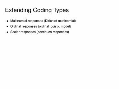
Extending Coding Types
• Multinomial responses (Dirichlet-multinomial)
• Ordinal responses (ordinal logistic model)
• Scalar responses (continuos responses)
71

Hierarchical and Multilvel Models• Assume several coding tasks
– e.g. multiple part-of-speech corpora
– e.g. multiple named-entity corpora (see Finkel and Manning2009)
– e.g. multiple language newswire categorization
– e.g. coref corpora in different genres or languages
• Estimate another level of priors
– e.g. for prevalence
– e.g. for priors on accuracy priors
• Common approach in social science models
• Even better pooled estimates if corpora are similar
• Multilevel models allow cross-cutting “hierarchies”
72

Semi-Supervision
• Easy to add in supervised cases with Bayesian models
– Gibbs sampling skips sampling for supervised cases
• May go half way by mixing in “gold standard” annotators
– e.g. fixed values from gold standard, or
– e.g. fixed high, but non-100% accuracies, or
– e.g. stronger high accuracy prior
• With accurate supervision, improves estimates
– for prevalence
– for annotator accuracies
– for pool of annotators
73

Multimodal (Mixture) Priors
• Model Mechanical Turk as mixture of spammers and hammers
• This is what the Mechanical Turk data suggests
• May also model covariance of sensitivity/specificity
– Use multivariate normal or T distribution
– with covariance matrix
– Covariance may also be estimated hierarchically (see Laffertyand Blei 2007)
74

Annotator and Item Random Effects• May add random effects for annotators
– amount of annotator training
– number of items annotated
– annotator native language
– annotator field of expertise
– intern, random undergrad, grad student, task designer
• Also for Items
– difficulty (already discussed)
– type of item being annotated
– frequency of item in a large corpus
– capitalization in named entity detection
• Use logistic regression with these predictors to model accuracies
75

Jointly Estimate Model and Annotations
• Can train a model with inferred (probabilistic) gold standard
• May use trained model like another annotator
• May be beneficial to train multiple different annotators
• (Raykar, Yu, Zhao, Jerebko, Florin, Hermosillo-Valadez, Bogoni, andMoy 2009)
76

Bayesian Estimation
and Inference
77

Bayesian Models
• Observed data: y; Model parameter(s): φ
• Likelihood function (or sampling distribution): p(y|φ)
• Prior: p(φ)
• Chain rule: p(y, φ) = p(y|φ) p(φ)
• Marginal (prior predictive distribution): p(y) =∫p(y|φ) p(φ) dφ
• Posterior: p(φ|y) calculated via Bayes’s rule
p(φ|y) = p(y, φ)/p(y)
= p(y|φ) p(φ)/p(y)
= p(y|φ) p(φ)/∫p(y|φ′)p(φ′)dφ′
∝ p(y|φ) p(φ)
78

Point Estimators are “Best” Guesses• Estimate parameters φ given observed data y• Maximum Likelihood Estimator (ML)
φ∗(y) = arg maxφ p(y|φ)
maximizes probability of observed data given parameters• Maximum a Posteriori (MAP) Estimate
φ(y) = arg maxφ p(φ|y) = arg maxφ p(y|φ) p(φ)
maximizes probability of parameters given observed data• If prior is constant, [i.e. p(φ) = c], then φ(y) = φ∗(y)
• Bayesian estimator (given mean square error loss)
φ(y) = E[φ] =∫φ p(φ|y) dφ
is expected parameter values given observed data• Bayesian estimates are unbiased by construction
[i.e. expected estimate is parameter’s true value]
79

Inference• Observed data y; New data y
• Posterior predictive distribution: p(y|y)
• Maximum likelihood approximation: p(y|y) ≈ p(y|φ∗(y))
• MAP approximation: p(y|y) ≈ p(y|φ(y))
• Bayesian point approximation: p(y|y) ≈ p(y|φ(y))
• Bayesian posterior predictive distribution
p(y|y) =∫p(y|φ) p(φ|y) dφ
averages over uncertainty in estimate of φ [i.e. p(φ|y)]
80

Bernoulli Distribution (Single Binary Trial)
• Outcome y ∈ {0, 1} [success=1, failure=0]
• Parameter θ ∈ [0, 1] is chance of success
• p(y|θ) = Bernoulli(y|θ) = θy (1− θ)1−y =
{θ if y = 11− θ if y = 0
• For N independent trials y = y1, . . . , yN , where yn ∈ {0, 1},
p(y|θ) =∏Nn=1 p(yn|θ)
=∏Nn=1 θ
yn (1− θ)1−yn
= θA(1− θ)B
where A =∑Nn=1 yn and B =
∑Nn=1(1− yn) = N −A
• x0 = 1 and xaxb = xa+b
81

Conjugate Priors
• Given a sampling distribution p(y|φ)
• Given a family of distributions F• The family F is conjugate for p(y|φ) if
prior p(φ) ∈ F implies posterior p(φ|y) ∈ F• Provides analytic form of posterior (vs. numerical approximation)
• Supports incremental updates
– Start with prior p(φ) ∈ F– After data y, have posterior p(φ|y) ∈ F– Use p(φ|y) as prior for new data y′
– New posterior is p(φ|y, y′) ∈ F– i.e. updating with y then y′ same as upating for y, y′ together
• Not necessary for Bayesian inference
82

Mean, Mode and Variance for Bernoulli
• Mean and Mode: E[Bern(θ)] = mode[Bern(θ)] = θ
• Variance: var[Bern(θ)] = θ (1− θ)
• Standard Deviation: sd[Bern(θ)] =√θ (1− θ)
• For discrete X with N outcomes x1, . . . , xN distributed pX(x)
– Mode (Max Value): mode[X] = arg maxNn=1 p(xn)
– Mean (Average Value): E[X] =∑Nn=1 p(xn) xn
– Variance: var[X] = E[X − E[X]] =∑Nn=1 p(xn) (xn − E[X])2
– Standard Deviation: sd[X] =√
var[X]
83

Beta Distribution• Outcome θ ∈ [0, 1]
• Parameters α, β > 0 [α− 1 prior successes; β − 1 failures]
• Continuous Density Function
p(θ|α, β) = Beta(θ|α, β)
= 1
B(α, β)θα−1 (1− θ)β−1
∝ θα−1 (1− θ)β−1
• Continuous densities p(θ) have p(θ) ≥ 0 and∫p(θ)dθ = 1
• Beta function B(α, β) =∫ 10θα−1 (1 − θ)β−1 dθ =
Γ(α+β)Γ(α)Γ(β)
• Γ(x) =∫∞0yx−1 exp(−y)dy is continuous generalization of factorial
i.e. Γ(n+ 1) = n! = n× (n− 1) × · · · × 2 × 1 for integer n ≥ 0
84

Beta ExamplesBeta (0.5, 0.5)
0 0.2 0.4 0.6 0.8 1
Beta (1, 1)
0 0.2 0.4 0.6 0.8 1
Beta (5, 5)
0 0.2 0.4 0.6 0.8 1
Beta (20, 20)
0 0.2 0.4 0.6 0.8 1
Beta (0.2, 0.8)
0 0.2 0.4 0.6 0.8 1
Beta (0.4, 1.6)
0 0.2 0.4 0.6 0.8 1
Beta (2, 8)
0 0.2 0.4 0.6 0.8 1
Beta (8, 32)
0 0.2 0.4 0.6 0.8 1
85

Mean, Mode and Variance for Beta
• Mean: E[Beta(α, β)] = αα+ β
• Variance: var[Beta(α, β)] =αβ
(α+ β)2 (α+ β + 1)
• Mode: mode[Beta(α, β)] =
α− 1
α+ β − 2if α > 1 and β > 1
undefined otherwise
86
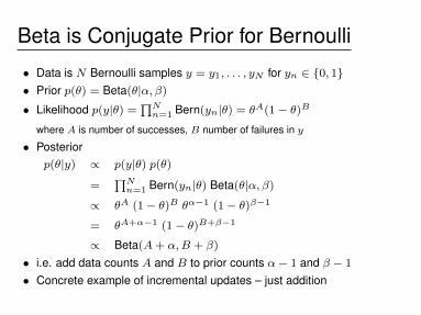
Beta is Conjugate Prior for Bernoulli
• Data is N Bernoulli samples y = y1, . . . , yN for yn ∈ {0, 1}• Prior p(θ) = Beta(θ|α, β)
• Likelihood p(y|θ) =∏Nn=1 Bern(yn|θ) = θA(1− θ)B
where A is number of successes, B number of failures in y
• Posteriorp(θ|y) ∝ p(y|θ) p(θ)
=∏Nn=1 Bern(yn|θ) Beta(θ|α, β)
∝ θA (1− θ)B θα−1 (1− θ)β−1
= θA+α−1 (1− θ)B+β−1
∝ Beta(A+ α,B + β)
• i.e. add data counts A and B to prior counts α− 1 and β − 1
• Concrete example of incremental updates – just addition
87

The End
88

References• References
– http://lingpipe-blog.com/
• Contact
• R/BUGS (Anon) Subversion Repository
svn co https://aliasi.devguard.com/svn/sandbox/hierAnno
89