Models for Network Graphs - University of Rochestergmateosb/ECE442/Slides/block_4...I Emphasis now...

Models for Network Graphs

Gonzalo MateosDept. of ECE and Goergen Institute for Data Science

University of Rochester

[email protected]

http://www.ece.rochester.edu/~gmateosb/

April 2, 2020

Network Science Analytics Models for Network Graphs 1

mailto:[email protected]

http://www.ece.rochester.edu/~gmateosb/

Random graph models

Random graph models

Small-world models

Network-growth models

Exponential random graph models

Case study: Modeling collaboration among lawyers


Why statistical graph modeling?

I Statistical inference typically conducted in the context of a model

⇒ Models key to transition from descriptive to inferential tasks

I In practice, graph models are used for a variety of reasons:

1) Mechanisms explaining properties observed on real-world networks

Ex: small-world effects, power-law degree distributions

2) Testing for ‘significance’ of a characteristic η(G ) in a network graph

Ex: is the observed average degree unusual or anomalous?

3) Alternative to the design-based framework for estimating η(G )

Ex: model-based, e.g., maximum likelihood estimation


Modeling network graphs

I So far the focus has been on network analysis methods to:

⇒ Collect relational data and construct network graphs

⇒ Characterize and summarize their structural properties

⇒ Obtain sample-based estimates of partially-observed structure

I Emphasis now on construction and use of models for network data

I Def: A model for a network graph is a collection

{Pθ(G ),G ∈ G : θ ∈ Θ}

I G is an ensemble of possible graphsI Pθ(·) is a probability distribution on G (often write P (·))I Parameters θ ranging over values in parameter space Θ


Model specification

I Richness of models derives from how we specify P(·)⇒ Methods range from the simple to the complex

1) Let P(·) be uniform on G, add structural constraints to GEx: Erdos-Renyi random graphs, generalized random graph models

2) Induce P(·) via application of simple generative mechanisms

Ex: small world, preferential attachment, copying models

3) Model structural features and their effect on G ’s topology

Ex: exponential random graph models

I Computational cost of associated inference algorithms relevant


Classical random graph models

I Assign equal probability on all undirected graphs of given order and size

I Specify collection GNv ,Ne of graphs G(V ,E) with |V | = Nv , |E | = Ne

I Assign P (G) =(NNe

)−1to each G ∈ GNv ,Ne , where N = |V (2)| =

(Nv2

)I Most common variant is the Erdos-Renyi random graph model Gn,p

⇒ Undirected graph on Nv = n vertices

⇒ Edge (u, v) present w.p. p, independent of other edges

I Simulation: simply draw N =(Nv

2

)≈ N2

v /2 i.i.d. Ber(p) RVs

I Inefficient when p ∼ N−1v ⇒ sparse graph, most draws are 0

I Skip non-edges drawing Geo(p) i.i.d. RVs, runs in O(Nv + Ne) time


Properties of Gn,p

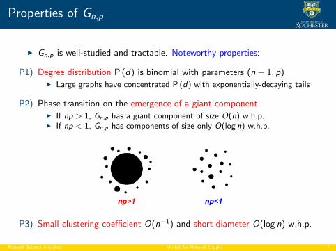
I Gn,p is well-studied and tractable. Noteworthy properties:

P1) Degree distribution P (d) is binomial with parameters (n − 1, p)I Large graphs have concentrated P (d) with exponentially-decaying tails

P2) Phase transition on the emergence of a giant componentI If np > 1, Gn,p has a giant component of size O(n) w.h.p.I If np < 1, Gn,p has components of size only O(log n) w.h.p.

np>1 np<1

P3) Small clustering coefficient O(n−1) and short diameter O(log n) w.h.p.


Generalized random graph models

I Recipe for generalization of Erdos-Renyi models

⇒ Specify G of fixed order Nv , possessing a desired characteristic

⇒ Assign equal probability to each graph G ∈ G

I Configuration model: fixed degree sequence {d(1), . . . , d(Nv )}I Size fixed under this model, since Ne = dNv/2 ⇒ G ⊂ GNv ,Ne

I Equivalent to specifying model via conditional distribution on GNv ,Ne

I Configuration models useful as reference, i.e., ‘null’ models

Ex: compare observed G with G ′ ∈ G having power law P (d)Ex: expected group-wise edge counts in modularity measure


Results on the configuration model

P1) Phase transition on the emergence of a giant componentI Condition depends on first two moments of given P (d)I Giant component has size O(Nv ) as in GNv ,p

I M. Molloy and B. Reed, “A critical point for random graphs with a givendegree sequence,” Random Struct. and Alg., vol. 6, pp. 161-180, 1995

P2) Clustering coefficient vanishes slower than in GNv ,p

I M. Newman et al, “Random graphs with arbitrary degree distrbutionsand their applications”, Physical Rev. E, vol. 64, p. 26,118, 2001

P3) Special case of given power-law degree distribution P (d) ∼ Cd−α

I For α ∈ (2, 3), short diameter O(logNv ) as in GNv ,p

I F. Chung and L. Lu, “The average distances in random graphs withgiven expected degrees,” PNAS, vol. 99, pp. 15,879-15,882, 2002


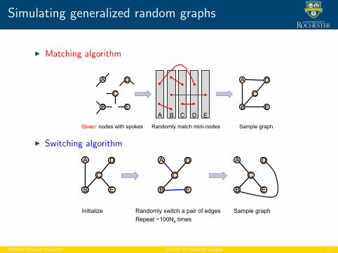
Simulating generalized random graphs

I Matching algorithm

A

C

D

EB

A B C D E

A

B

C

D

E

Given: nodes with spokes Randomly match mini-nodes Sample graph

I Switching algorithm

A

B

C

D

Initialize

A

B

Sample graph

A

B

D

E

Randomly switch a pair of edges

E

C

Repeat ~100Ne times

D

C

E


Task 1: Model-based estimation in network graphs

I Consider a sample G∗ of a population graph G (V ,E )

⇒ Suppose a given characteristic η(G ) is of interest

⇒ Q: Useful estimate η = η(G∗) of η(G )?

I Statistical inference in sampling theory via design-based methods

⇒ Only source of randomness is due to the sampling design

I Augment this perspective to include a model-based componentI Assume G drawn uniformly from the collection G, prior to sampling

I Inference on η(G ) should incorporate both randomness due to

⇒ Selection of G from G and sampling G∗ from G


Example: size of a “hidden population”

I Directed graph G (V ,E ), V the members of the hidden population

⇒ Graph describing willingness to identify other members

⇒ Arc (i , j) when ask individual i , mentions j as a member

I For given V , model G as drawn from a collection G of random graphs

⇒ Independently add arcs between vertex pairs w.p. pG

I Graph G∗ obtained via one-wave snowball sampling, i.e., V ∗ = V ∗0 ∪ V ∗1⇒ Initial sample V ∗0 obtained via BS from V with probability p0

I Consider the following RVs of interestI N = |V ∗0 |: size of the initial sampleI M1: number of arcs among individuals in V ∗0I M2: number of arcs from individuals in V ∗0 to individuals in V ∗1

I Snowball sampling yields measurements n,m1, and m2 of these RVs


Method of moments estimator

I Method of moments: now Aij = I {(i , j) ∈ E} also a RV

E [N] = E

[∑i

I {i ∈ V ∗0 }

]= Nvp0= n

E [M1] = E

∑j

∑i 6=j

I {i ∈ V ∗0 }I {j ∈ V ∗0 }Aij

= Nv (Nv − 1)p20pG= m1

E [M2] = E

∑j

∑i 6=j

I {i ∈ V ∗0 }I {j /∈ V ∗0 }Aij

= Nv (Nv − 1)p0(1− p0)pG= m2

I Expectation w.r.t. randomness in selecting G and sample V ∗0 . Solution:

p0 =m1

m1 + m2, pG =

m1(m1 + m2)

n[(n − 1)m1 + nm2], and Nv = n

(m1 + m2

m1

)⇒ Same estimates for p0 and Nv as in the design-based approach


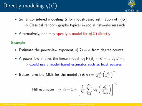
Directly modeling η(G )

I So far considered modeling G for model-based estimation of η(G )

⇒ Classical random graphs typical in social networks research

I Alternatively, one may specify a model for η(G ) directly

Example

I Estimate the power-law exponent η(G ) = α from degree counts

I A power law implies the linear model log P (d) = C − α log d + ε

⇒ Could use a model-based estimator such as least squares

I Better form the MLE for the model f (d ;α) = α−1dmin

(d

dmin

)−α

Hill estimator ⇒ α = 1 +

[1

Nv

Nv∑i=1

log

(didmin

)]−1


Task 2: Assessing significance in network graphs

I Consider a graph G obs derived from observations

I Q: Is a structural characteristic η(G obs) significant, i.e., unusual?

⇒ Assessing significance requires a frame of reference, or null model

⇒ Random graph models often used in setting up such comparisons

I Define collection G, and compare η(G obs) with values {η(G ) : G ∈ G}⇒ Formally, construct the reference distribution

Pη,G(t) =|{G ∈ G : η(G ) ≤ t}|

|G|

I If η(G obs) found to be sufficiently unlikely under Pη,G(t)

⇒ Evidence against the null H0: G obs is a uniform draw from G


Example: Zachary’s karate club

I Zachary’s karate club has clustering coefficient cl(G obs) = 0.2257

⇒ Random graph models to assess whether the value is unusual

I Construct two ‘comparable’ abstract frames of reference

1) Collection G1 of random graphs with same Nv = 34 and Ne = 782) Add the constraint that G2 has the same degree distribution as G obs

I |G1| ≈ 8.4× 1096 and |G2| much smaller, but still large

⇒ Enumerating G1 intractable to obtain Pη,G1(t) exactly

I Instead use simulations to approximate both distributions

⇒ Draw 10,000 uniform samples G from each G1 and G2⇒ Calculate η(G ) = cl(G ) for each sample, plot histograms


Example: Zachary’s karate club (cont.)

I Plot histograms to approximate the distributions1

Den

sity

0.05 0.10 0.15 0.20 0.25

010

20

Clustering Coefficient

Den

sity

0.05 0.10 0.15 0.20 0.25

010

20

Fig. 6.1 Histograms of clustering coefficients clT (G) for random graphs of order Nv = 34, gen-erated uniformly from those with the same number of edges Ne (top, in red) and the same degreedistribution (bottom, in blue) as in the karate club network.

Copyright 2009 Springer Science+Business Media, LLC. These figures may be used for noncom-mercial purposes as long as the source is cited: Kolaczyk, Eric D. Statistical Analysis of NetworkData: Methods and Models (2009) Springer Science+Business Media LLC.

1

Den

sity

0.05 0.10 0.15 0.20 0.25

010

20


Den

sity

0.05 0.10 0.15 0.20 0.25

010

20



1

Den

sity

0.05 0.10 0.15 0.20 0.25

010

20


Den

sity

0.05 0.10 0.15 0.20 0.25

010

20



Same order and size Same degree distribution

I Unlikely to see a value cl(G obs) = 0.2257 under both graph models

Ex: only 3 out of 10,000 samples from G1 had cl(G ) > 0.2257

I Strong evidence to reject G obs obtained as sample from G1 or G2


Task 3: Detecting network motifs

I Related use of random graph models is for detecting network motifs

⇒ Find the simple ‘building blocks’ of a large complex network

I Def: Network motifs are small subgraphs occurring far more frequently ina given network than in comparable random graphs

I Ex: there are L3 = 13 different connected 3-vertex subdigraphs

I Let Ni be the count in G of the i-th type k-vertex subgraph, i = 1, . . . , Lk

⇒ Each value Ni can be compared to a suitable reference PNi ,G

⇒ Subgraphs for which Ni is extreme are declared as network motifsNetwork Science Analytics Models for Network Graphs 18

Example: AIDS blog network

I AIDS blog network G obs with Nv = 146 bloggers and Ne = 183 links

⇒ Examined evidence for motifs of size k = 3 and 4 vertices4

Fig. 1.4 AIDS Blog Network

2

Fig. 6.2 Three-vertex motif discovered for the AIDS blog network.

3

Fig. 6.3 Four-vertex motifs discovered for the AIDS blog network.

3-vertex motif

4-vertex motifs

I Simulated 10,000 digraphs using a switching algorithm

⇒ Fixed in- and out-degree sequences, mutual edges as in G obs

⇒ Constructed approximate reference distributions PNi ,G(t)

I Ex: two bloggers with a mutual edge and a common ‘authority’


Challenges in detecting motifs

I Individual motifs frequently overlap with other copies of itself

⇒ May require them to be frequent and mostly disjoint subgraphs

I With large graphs come significant computational challenges

⇒ Number of different potential motifs Lk grows fast with k

Ex: Connected subdigraphs L3 = 13, L4 = 199, L5 = 9364

I May sample subgraphs H along with the HT estimation framework

Ni =∑

H of type i

π−1H


Small-world models

Random graph models

Small-world models





Models for real-world networks

I Arguably the most important innovation in modern graph modeling

Traditional random

graph models

Models mimicking observed

``real-world’’ properties

Transition


A “small” world?

I Six degrees of separation popularized by a play [Guare’90]

⇒ Short paths between us and everyone else on the planet

⇒ Term relatively new, the concept has a long history

I Traced back to F. Karinthy in the 1920s

⇒ ‘Shrinking’ modern world due to increased human connectedness

⇒ Challenge: find someone whose distance from you is > 5

⇒ Inspired by G. Marconi’s Nobel prize speech in 1909

I First mathematical treatment [Kochen-Pool’50]

⇒ Formally modeled the mechanics of social networks

⇒ But left ‘degrees of separation’ question unanswered

I Chain of events led to a groundbreaking experiment [Milgram’67]


Milgram’s experiment

I Q1: What is the typical geodesic distance between two people?

⇒ Experiment on the global friendship (social) network

⇒ Cannot measure in full, so need to probe explicitly

I S. Milgram’s ingenious small-world experiment in 1967I 296 letters sent to people in Wichita, KS and Omaha, NEI Letters indicated a (unique) contact person in Boston, MAI Asked them to forward the letter to the contact, following rules

I Def: friend is someone known on a first-name basis

Rule 1: If contact is a friend then send her the letter; else

Rule 2: Relay to friend most-likely to be a contact’s friend

I Q2: How many letters arrived? How long did they take?


Milgram’s experimental results

I 64 of 296 letter reached the destination, average path length ¯ = 6.2

⇒ Inspiring Guare’s ‘6 degrees of separation’

I Conclusion: short paths connect arbitrary pairs of people

I S. Milgram, “The small-world problem,” Psychology Today, vol. 2,pp. 60-67, 1967


Moment to reflect

I Milgram demonstrated that short paths are in abundance

I Q: Is the small-world theory reasonable? Sure, e.g., assumes:I We have 100 friends, each of them has 100 other friends, . . .I After 5 degrees we get 1010 friends > twice the Earth’s population

Friends

Friends of friends

Friends

Friends of friends

I Not a realistic model of social networks exhibiting:

⇒ Homophily [Lazarzfeld’54]

⇒ Triadic closure [Rapoport’53]

I Q: How can networks be highly-structured locally and globally small?


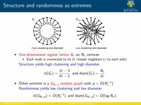
Structure and randomness as extremes

High clustering and diameter Low clustering and diameter

Gr Gn,p

I One-dimensional regular lattice Gr on Nv verticesI Each node is connected to its 2r closest neighbors (r to each side)

Structure yields high clustering and high diameter

cl(Gr ) =3r − 3

4r − 2and diam(Gr ) =

Nv

2r

I Other extreme is a GNv ,p random graph with p = O(N−1v )

Randomness yields low clustering and low diameter

cl(GNv ,p) = O(N−1v ) and diam(GNv ,p) = O(logNv )


The Watts-Strogatz model

I Small-world model: blend of structure with little randomness

S1: Start with regular lattice that has desired clustering

S2: Introduce randomness to generate shortcuts in the graph

⇒ Each edge is randomly rewired with (small) probability p

I Rewiring interpolates between the regular and random extremes


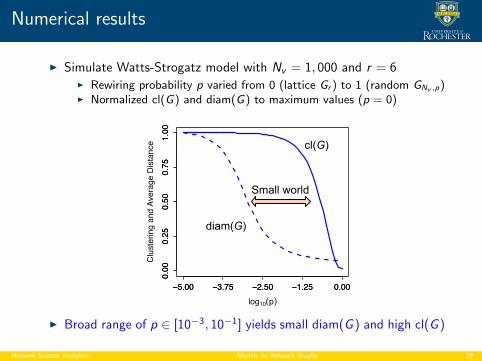
Numerical results

I Simulate Watts-Strogatz model with Nv = 1, 000 and r = 6I Rewiring probability p varied from 0 (lattice Gr ) to 1 (random GNv ,p)I Normalized cl(G) and diam(G) to maximum values (p = 0)

5

−5.00 −3.75 −2.50 −1.25 0.00

0.00

0.25

0.50

0.75

1.00

log10(p)

Clu

ster

ing

and

Aver

age

Dis

tanc

e

−5.00 −3.75 −2.50 −1.25 0.00

0.00

0.25

0.50

0.75

1.00

Fig. 6.5 Plot of the clustering coefficient cl(G) (solid) and average geodesic distance l (dashed),as a function of the rewiring probability p for a Watts-Strogatz small-world model. Results areaverages based on 1,000 simulation trials.

cl(G)

diam(G)

Small world

I Broad range of p ∈ [10−3, 10−1] yields small diam(G ) and high cl(G )


Closing remarks

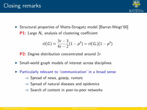
I Structural properties of Watts-Strogatz model [Barrat-Weigt’00]

P1: Large Nv analysis of clustering coefficient

cl(G ) ≈ 3r − 3

4r − 2(1− p3) = cl(Gr )(1− p3)

P2: Degree distribution concentrated around 2r

I Small-world graph models of interest across disciplines

I Particularly relevant to ‘communication’ in a broad sense

⇒ Spread of news, gossip, rumors

⇒ Spread of natural diseases and epidemics

⇒ Search of content in peer-to-peer networks



Random graph models

Small-world models





Time-evolving networks

I Many networks grow or otherwise evolve in time

Ex: Web, scientific citations, Twitter, genome . . .

I General approach to model construction mimicking network growthI Specify simple mechanisms for network dynamicsI Study emergent structural characteristics as time t →∞

I Q: Do these properties match observed ones in real-world networks?

I Two fundamental and popular classes of growth processes

⇒ Preferential attachment models

⇒ Copying models

I Tenable mechanisms for popularity and gene duplication, respectively


Preferential attachment model

I Simple model for the creation of e.g., links among Web pages

I Vertices are created one at a time, denoted 1, . . . ,Nv

I When node j is created, it makes a single arc to i , 1 ≤ i < j

I Creation of (j , i) governed by a probabilistic rule:I With probability p, j links to i chosen uniformly at randomI With probability 1− p, j links to i with probability ∝ d in

i

I The resulting graph is directed, each vertex has doutv = 1

I Preferential attachment model leads to “rich-gets-richer” dynamics

⇒ Arcs formed preferentially to (currently) most popular nodes

⇒ Prob. that i increases its popularity ∝ i ’s current popularity


Preferential attachment yields power laws

TheoremThe preferential attachment model gives rise to a power-law in-degreedistribution with exponent α = 1 + 1

1−p , i.e.,

P(d in = d

)∝ d−(1+ 1

1−p )

I Key: “j links to i with probability ∝ d ini ” equivalent to copying, i.e.,

“j chooses k uniformly at random, and links to i if (k, i) ∈ E”

I Reflect: Copy other’s decision vs. independent decisions in Gn,p

I As p → 0 ⇒ Copying more frequent ⇒ Smaller α→ 2I Intuitive: more likely to see extremely popular pages (heavier tail)


The Barabasi-Albert model

I Barabasi-Albert (BA) model is for undirected graphs

I Initial graph GBA(0) of Nv (0) vertices and Ne(0) edges (t = 0)

I For t = 1, 2, . . . current graph GBA(t − 1) grows to GBA(t) by:I Adding a new vertex u of degree du(t) = m ≥ 1I The m new edges are incident to m different vertices in GBA(t − 1)I New vertex u is connected to v ∈ V (t − 1) w.p.

P ((u, v) ∈ E (t)) =dv (t − 1)∑v ′ dv ′(t − 1)

I Vertices connected to u preferentially towards higher degrees

⇒ GBA(t) has Nv (t) = Nv (0) + t and Ne(t) = Ne(0) + tm

I A. Barabasi and R. Albert, “Emergence of scaling in randomnetworks,” Science, vol. 286, pp. 509-512, 1999


Linearized chord diagram

I BA model ambiguous in how to select m vertices ∝ to their degree

⇒ Joint distribution not specified by marginal on each vertex

I Linearzied chord diagram (LCD) model removes ambiguities

I For m = 1, start with GLCD(0) consisting of a vertex with a self-loop

I For t = 1, 2, . . . current graph GLCD(t − 1) grows to GLCD(t) by:I Adding a new vertex vt with an edge to vs ∈ V (t)I Vertex vs , 1 ≤ s ≤ t is chosen w.p.

P (s = j) =

{dvj (t−1)2t−1 , if 1 ≤ j ≤ t − 1,1

2t−1 , if j = t

I For m > 1 simply run the above process m times for each tI Collapse all created vertices into a single one, retaining edges

I A. Bollobas et al, “The degree sequence of a scale-free random graphprocess,” Random Struct. and Alg., vol. 18, pp. 279-290, 2001


Properties of the LCD model

P1) The LCD model allows for loops and multi-edges, occurring rarely

P2) GLCD(t) has power-law degree distribution with α = 3, as t →∞

P3) The BA model yields connected graphs if GBA(0) connected

⇒ Not true for the LCD model, but GLCD(t) connected w.h.p.

P4) Small-world behavior

diam(GLCD(t)) =

{O(logNv (t)), m = 1

O( logNv (t)log logNv (t)

), m > 1

P5) Unsatisfactory clustering, since small for m > 1

E [cl(GLCD(t))] ≈ m − 1

8

(logNv (t))2

Nv (t)

⇒ Marginally better than O(N−1v ) in classical random graphs


Copying models

I Copying is another mechanism of fundamental interest

Ex: gene duplication to re-use information in organism’s evolution

I Different from preferential attachment, but still results in power laws

I Initialize with a graph GC (0) (t = 0)

I For t = 1, 2, . . . current graph GC (t − 1) grows to GC (t) by:I Adding a new vertex uI Choosing vertex v ∈ V (t − 1) with uniform probability 1

Nv (t−1)I Joining vertex u with v ’s neighbors independently w.p. p

I Case p = 1 leads to full duplication of edges from an existing node

I F. Chung et al, “Duplication models for biological networks,”Journal of Computational Biology, vol. 10, pp. 677-687, 2003


Asymptotic degree distribution

I Degree distribution tends to a power law w.h.p. [Chung et al’03]

⇒ Exponent α is the plotted solution to the equation

p(α− 1) = 1− pα−16

0.2 0.4 0.6 0.8 1.0

12

34

56

p

α

Fig. 6.6 Power-law exponent α , as a function of p, for the copying model of Chung, Lu, Dewey,and Galas [89], as given by the expression in equation (6.19).I Full duplication does not lead to power-law behavior; but does if

⇒ Partial duplication performed a fraction q ∈ (0, 1) of times


Fitting network growth models

I Most common practical usage of network growth models is predictive

Goal: compare characteristics of G obs and G (t) from the models

I Little attempt to date to fit network growth models to data

⇒ Expected due to simplicity of such models

⇒ Still useful to estimate e.g., the duplication probability p

I To fit a model ideally would like to observe a sequence {G obs(τ)}tτ=1

⇒ Unfortunately, such dynamic network data is still fairly elusive

I Q: Can we fit a network growth model to a single snap-shot G obs?

I A: Yes, if we leverage the Markovianity of the growth process


Duplication-attachment models

I Similar to all network growth models described so far, suppose:

As1: A single vertex is added to G(t − 1) to create G(t); andAs2: The manner in which it is added depends only on G(t − 1)

I In other words, we assume {G (t)}∞t=0 is a Markov chain

I Let graph δ(G (t), v) be obtained by deleting v and its edges from G (t)

I Def: vertex v is removable if G (t) can be obtained from δ(G (t), v) viacopying. If G (t) has no removable vertices, we call it irreducible

I The class of duplication-attachment (DA) models satisfies:

(i) The initial graph G(0) is irreducible; and(ii) Pθ(G(t)

∣∣G(t − 1)) > 0⇔ G(t) obtained by copying a vertex in G(t − 1)

I C. Wiuf et al, “A likelihood approach to analysis of network data,”PNAS, vol. 103, pp. 7566-7570, 2006


Example: reducible graph

A

B

C

D

A

B

C

D

A

B

C

D

�(G(t), vA) �(G(t), vB)G(t)

I Vertex vA is removable (likewise vc by symmetry)

⇒ Obtain G (t) from δ(G (t, va)) by copying vc

I This implies that G (t) is reducible

⇒ Notice though that vB or vD are not removable


MLE for DA model parameters

I Suppose that G obs = G (t) represents the observed network graph

I The likelihood for the parameter θ is recursively given by

L (θ;G (t)) =1

t

∑v∈RG(t)

Pθ(G (t)

∣∣ δ(G (t), v))L (θ; δ(G (t), v))

⇒ RG(t) is the set of all removable nodes in G (t)

I The MLE for θ is thus defined as

θ = arg maxθL (θ;G (t))

⇒ Computing L (θ;G (t)) non-trivial, even for modest-size graphs

I Monte Carlo methods to approximate L (θ;G (t)) [Wiupf et al’06]

⇒ Open issues: vector θ, other growth models, scalability



Random graph models

Small-world models





Statistical network graph models

I Good statistical network graph models should be [Robbins-Morris’07]:

⇒ Estimable from and reasonably representative of the data

⇒ Theoretically plausible about the underlying network effects

⇒ Discriminative among competing effects to best explain the data

I Network-based versions of canonical statistical models

⇒ Regression models - Exponential random graph models (ERGMs)

⇒ Latent variable models - Latent network models

⇒ Mixture models - Stochastic block models

I Focus here on ERGMs, also known as p∗ models

I G. Robbins et al., “An introduction to exponential random graph (p∗)models for social networks,” Social Networks, vol. 29, pp. 173-191, 2007


Exponential family

I Def: discrete random vector Z ∈ Z belongs to an exponential family if

Pθ(Z = z) = exp{θ>g(z)− ψ(θ)

}I θ ∈ Rp is a vector of parameters and g : Z 7→ Rp is a functionI ψ(θ) is a normalization term, ensuring

∑z∈Z Pθ(z) = 1

I Ex: Bernoulli, binomial, Poisson, geometric distributions

I For continuous exponential families, the pdf has an analogous form

Ex: Gaussian, Pareto, chi-square distributions

I Exponential families share useful algebraic and geometric properties

⇒ Mathematically convenient for inference and simulation


Exponential random graph model

I Let G (V ,E ) be a random undirected graph, with Yij := I {(i , j) ∈ E}I Matrix Y = [Yij ] is the random adjacency matrix, y = [yij ] a realization

I An ERGM specifies in exponential family form the distribution of Y, i.e.,

Pθ(Y = y) =

(1

κ(θ)

)exp

{∑H

θHgH(y)

}, where

(i) each H is a configuration, meaning a set of possible edges in G ;(ii) gH(y) is the network statistic corresponding to configuration H

gH(y) =∏yij∈H

yij = I {H occurs in y}

(iii) θH 6= 0 only if all edges in H are conditionally dependent; and(iv) κ(θ) is a normalization constant ensuring

∑y Pθ(y) = 1


Discussion

I Graph order Nv is fixed and given, only edges are random

⇒ Assumed unweighted, undirected edges. Extensions possible

I ERGMs describe random graphs ‘built-on’ localized patternsI These configurations are the structural characteristics of interestI Ex: Are there reciprocity effects? Add mutual arcs as configurationsI Ex: Are there transitivity effects? Consider triangles

I (In)dependence is conditional on all other variables (edges) in G

⇒ Control configurations relevant (i.e., θH 6= 0) to the model

I Well-specified dependence assumptions imply particular model classes


A general framework for model construction

I In positing an ERGM for a network, one implicitly follows five steps

⇒ Explicit choices connecting hypothesized theory to data analysis

Step 1: Each edge (relational tie) is regarded as a random variable

Step 2: A dependence hypothesis is proposed

Step 3: Dependence hypothesis implies a particular form to the model

Step 4: Simplification of parameters through e.g., homogeneity

Step 5: Estimate and interpret model parameters


Example: Bernoulli random graphs

I Assume edges present independently of all other edges (e.g., in Gn,p)

⇒ Simplest possible (and unrealistic) dependence assumption

I For each (i , j), we assume Yij independent of Yuv , for all (u, v) 6= (i , j)

⇒ θH = 0 for all H involving two or more edges

I Edge configurations i.e., gH(y) = yij relevant, and the ERGM becomes

Pθ(Y = y) =

(1

κ(θ)

)exp

∑i,j

θijyij

I Specifies that edge (i , j) present independently, with probability

pij =exp(θij)

1 + exp(θij)


Constraints on parameters: homogeneity

I Too many parameters makes estimation infeasible from single y

⇒ Under independence have N2v parameters {θij}. Reduction?

I Homogeneity across all G , i.e., θij = θ for all (i , j) yields

Pθ(Y = y) =

(1

κ(θ)

)exp {θL(y)}

I Relevant statistic is the number of edges observed L(y) =∑

i,j yij

I ERGM identical to Gn,p, where p =exp θ

1 + exp θ

Ex: suppose we know a priori that vertices fall in two sets

I Can impose homogeneity on edges within and between sets, i.e.,

Pθ(Y = y) =

(1

κ(θ)

)exp {θ1L1(y) + θ12L12(y) + θ2L2(y)}


Example: Markov random graphs

I Markov dependence notion for network graphs [Frank-Strauss’86]I Assumes two ties are dependent if they share a common nodeI Edge status Yij dependent on any other edge involving i or j

TheoremUnder homogeneity, G is a Markov random graph if and only if

Pθ(Y = y) =

(1

κ(θ)

)exp

{Nv−1∑k=1

θkSk(y) + θτT (y)

}, where

Sk(y) is the number of k-stars, and T (y) the number of triangles

1-star=edge 2-star 3-star Triangle


Alternative statistics

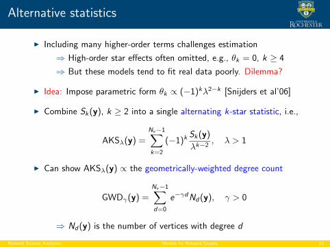
I Including many higher-order terms challenges estimation

⇒ High-order star effects often omitted, e.g., θk = 0, k ≥ 4

⇒ But these models tend to fit real data poorly. Dilemma?

I Idea: Impose parametric form θk ∝ (−1)kλ2−k [Snijders et al’06]

I Combine Sk(y), k ≥ 2 into a single alternating k-star statistic, i.e.,

AKSλ(y) =Nv−1∑k=2

(−1)kSk(y)

λk−2, λ > 1

I Can show AKSλ(y) ∝ the geometrically-weighted degree count

GWDγ(y) =Nv−1∑d=0

e−γdNd(y), γ > 0

⇒ Nd(y) is the number of vertices with degree d


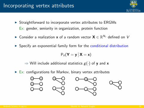
Incorporating vertex attributes

I Straightforward to incorporate vertex attributes to ERGMs

Ex: gender, seniority in organization, protein function

I Consider a realization x of a random vector X ∈ RNv defined on V

I Specify an exponential family form for the conditional distribution

Pθ(Y = y∣∣X = x)

⇒ Will include additional statistics g(·) of y and x

I Ex: configurations for Markov, binary vertex attributes


Estimating ERGM parameters

I MLE for the parameter vector θ in an ERGM is

θ = arg maxθ

{θ>g(y)− ψ(θ)

}, where ψ(θ) := log κ(θ)

I Optimality condition yields

g(y) = ∇ψ(θ)|θ=θ

I Using also that Eθ[g(Y)] = ∇ψ(θ), the MLE solves

Eθ[g(Y)] = g(y)

I Unfortunately ψ(θ) cannot be computed except for small graphs

⇒ Involves a summation over 2(Nv2 ) values of y for each θ

⇒ Numerical methods needed to obtain approximate values of θ


Proof of E [g(Y)] = ∇ψ(θ)

I The pmf of Y is Pθ(Y = y) = exp{θ>g(y)− ψ(θ)

}, hence

Eθ[g(Y)] =∑y

g(y)Pθ(Y = y)

=∑y

g(y) exp{θ>g(y)− ψ(θ)

}

I Recall ψ(θ) = log∑

y exp{θ>g(y)

}and use the chain rule

∇ψ(θ) =

∑y g(y) exp

{θ>g(y)

}∑

y exp{θ>g(y)

} =

∑y g(y) exp

{θ>g(y)

}expψ(θ)

=∑y

g(y) exp{θ>g(y)− ψ(θ)

}I The red and blue sums are identical ⇒ Eθ[g(Y)] = ∇ψ(θ) follows


Markov chain Monte Carlo MLE

I Idea: for fixed θ0, maximize instead the log-likelihood ratio

r(θ,θ0) = `(θ)− `(θ0) = (θ − θ0)>g(y)− [ψ(θ)− ψ(θ0)]

I Key identity: will show that

exp {ψ(θ)− ψ(θ0)} = Eθ0[exp

{(θ − θ0)>g(Y)

}]I Markov chain Monte Carlo MLE algorithm to search over θ

Step 1: draw samples Y1, . . . ,Yn from the ERGM under θ0

Step 2: approximate the above Eθ0 [·] via sample averaging

Step 3: the logarithm of the result approximates ψ(θ)− ψ(θ0)

Step 4: evaluate an ≈ log-likelihood ratio r(θ,θ0)

I For large n, the maximum value found approximates the MLE θ


Derivation of key identity

I Recall expψ(θ) =∑

y exp{θ>g(y)

}to write

exp {ψ(θ)− ψ(θ0)} =

∑y exp

{θ>g(y)

}expψ(θ0)

I Multiplying and dividing by exp{θ>0 g(y)

}> 0 yields

exp {ψ(θ)− ψ(θ0)} =∑y

exp{

(θ−θ0)>g(y)}×

exp{θ>0 g(y)

}expψ(θ0)

=∑y

exp{

(θ − θ0)>g(y)}

Pθ0(Y = y)

= Eθ0[exp

{(θ − θ0)>g(Y)

}]I Used exp

{θ>0 g(y)− ψ(θ0)

}is the exponential family pmf Pθ0(Y = y)


Model goodness-of-fit

I Best fit chosen from a given class of models . . .

may not be a good fit to the data if model class not rich enough

I Assessing goodness-of-fit for ERGMs

Step 1: simulate numerous random graphs from the fitted model

Step 2: compare high-level characteristics with those of G obs

Ex: distributions of degree, centrality, diameter

I If significant differences found in G obs , conclude

⇒ Systematic gap between specified model class and data

⇒ Lack of goodness-of-fit

I Take home: model specification for ERGMs highly nontrivial

⇒ Goodness-of-fit diagnostics can play key facilitating role


Case study

Random graph models

Small-world models





Lawyer collaboration network

I Network G obs of working relationships among lawyers [Lazega’01]I Nodes are Nv = 36 partners, edges indicate partners worked together

7

1

2

34

5

6

7

8

9

10

11

12

13

14

15

1617

18

19

20

21

22

23

24

2526

27

28

29

3031

32

33

3435

36

Fig. 6.7 Visualization of Lazega’s network of collaborative working relationships among lawyers.Vertices represent partners and are labeled according to their seniority. Vertex shapes (i.e., triangle,square, or pentagon) indicate three different office locations, while vertex colors correspond to thetype of practice (i.e., litigation (red) or corporate (cyan)). Edges indicate collaboration betweenpartners. There are three female partners (i.e., those with seniority labels 27, 29, and 34); the restare male. Data courtesy of Emmanuel Lazega.

I Data includes various node-level attributes:I Seniority (node labels indicate rank ordering)I Office location (triangle, square or pentagon)I Type of practice, i.e., litigation (red) and corporate (cyan)I Gender (three partners are female labeled 27, 29 and 34)

I Goal: study cooperation among social actors in an organization


Modeling lawyer collaborations

I Assess network effects S1(y) = Ne and alternating k-triangles statistic

AKTλ(y) = 3T1(y) +Nv−2∑k=2

(−1)k+1Tk(y)

λk−1

⇒ Tk(y) counts sets of k individual triangles sharing a common base

I Test the following set of exogenous effects:

h(1)(xi , xj) = seniorityi + seniorityj , h(2)(xi , xj) = practicei + practicej

h(3)(xi , xj) = I{

practicei = practicej}, h(4)(xi , xj) = I

{genderi = genderj

}h(5)(xi , xj) = I {officei = officej}, h(xi , xj) := [h(1)(xi , xj), . . . , h

(5)(xi , xj)]T

I Resulting ERGM

Pθ,β(Y = y|X = x) =1

κ(θ,β)exp

{θ1S1(y) + θ2AKTλ(y) + βTg(y, x)

}g(y, x) =

∑i,j

yijh(xi , xj)


Model fitting result

I Fitting results using the MCMC MLE approach

⇒ Standard errors heuristically obtained via asymptotic theory

I Identified factors that may increase odds of cooperation

Ex: same practice, gender and office location double odds

I Strong evidence for transitivity effects since θ2 � se(θ2)

⇒ Something beyond basic homophily explaining such effects


Assessing goodness-of-fit

I Assess goodness-of-fit to G obs

I Sample from fitted ERGM

I Compared distributions ofI DegreeI Edge-wise shared partnersI Geodesic distance

I Plots show good fit overall

8

0 4 8 13 18

0.00

0.05

0.10

0.15

0.20

Degree

Prop

ortio

n of

Nod

es

0 3 6 9

0.0

0.1

0.2

0.3

0.4

Edge−wise Shared PartnersPr

opor

tion

of E

dges

1 3 5 7

0.0

0.1

0.2

0.3

0.4

0.5

Minimum Geodesic Distance

Prop

ortio

n of

Dya

ds

Fig. 6.8 Goodness-of-fit plots comparing original Lazega lawyer network and 100 realizationsfrom the model in (6.43), with the parameters in Table 6.1. Comparisons are made based on thedistribution of degree, edge-wise shared partners, and geodesic distance over the 100 realizations,represented by box-plots and curves showing 10-th and 90-th quantiles – both in green. Values forthe Lazega network itself are shown with solid blue lines. In the distribution of geodesic distancesbetween pairs, the rightmost box-plot is separate and corresponds to the proportion of nonreachablepairs.


Glossary

I Network graph model

I Random graph models

I Configuration model

I Matching algorithm

I Switching algorithm

I Model-based estimation

I Assessing significance

I Reference distribution

I Network motif

I Small-world network

I Decentralized search

I Watts-Strogatz model

I Time-evolving network

I Network-growth models

I Preferential attachment

I Barabasi-Albert model

I Copying models

I Exponential family

I Exponential random graph models

I Configurations

I Network statistic

I Homogeneity

I Markov random graphs


Models for Network Graphs - University of Rochestergmateosb/ECE442/Slides/block_4...I Emphasis now...

Documents

Transcript of Models for Network Graphs - University of Rochestergmateosb/ECE442/Slides/block_4...I Emphasis now...