Models for Banks' Loan Impairment Charges in Stress Tests ...€¦ · Models for Banks' Loan...

57

Models for Banks' Loan Impairment Charges in Stress Tests of the Financial System

Kim Abildgren, Economics, and Jannick Damgaard, Financial Markets1

1. INTRODUCTION AND SUMMARY

In an international perspective, the financial crisis has led to renewed focus on development of models for assessing financial stability. A case in point is macro stress testing of banks' capitalisation.

A key element of macro stress testing is to calculate banks' loan im-pairment charges in macroeconomic scenarios with severe negative shocks to the economy. Loan impairment charges are often the decisive factor determining the banks' financial performance and excess capital adequacy in periods of unfavourable macroeconomic developments. This is because credit is at the core of banking activities, so naturally it is also the major source of potential losses.

The current accounting principles entail considerable cyclical variation in the banks' loan impairment charge ratios. Loan impairment charges are relatively high in years when the economy is slowing down and bank earnings are under pressure, while they are relatively low in years with high economic growth and sound bank earnings. This link between the banks' loan impairment charges and the business cycle should be re-flected in the models used for calculating loan impairment charges in stress tests.

Detailed statistics on the banks' loan impairment charges are very scarce. This article presents approximate calculations of the banks' loan impairment charges by industry and sector since 1992, based on the Dan-ish Financial Supervisory Authority's statistics on the banks' losses and accumulated loan impairment charges. For all industries/sectors, loan im-pairment charges tend to be made 1-2 years before realisation of the losses. Moreover, for all industries the loan impairment charge ratios were relatively high in connection with the economic crisis in the early 1990s and the financial crisis from 2008 onwards. However, the level of

1 The authors thank Christian Møller Dahl, The University of Southern Denmark, for valuable sugges-

tions and comments in connection with the preparation of the analyses in this article. Any remaining deficiencies in the article as well as views and conclusions are solely the responsibility of the authors.

Monetary Review, 1st Quarter 2012 - Part 2

58

loan impairment charges in crisis periods compared with non-crisis periods varies strongly across industries. Very high loan impairment charge ratios were observed for particularly agriculture, etc. construc-tion, etc. and real estate, etc. in the crisis years.

All else equal, loan impairment charges under the current accounting principles increase the banks' lending capacity during booms and reduce their lending capacity during recessions. Hence the accounting rules for loan impairment charges are procyclical, i.e. they amplify cyclical fluc-tuations. In the wake of the most recent financial crisis it has therefore been discussed whether there is a need to amend the accounting rules so as to ensure that banks build up buffers in good times against losses in bad times.

There are various approaches to modelling the banks' loan impairment charges in connection with macro stress testing of the financial system. These approaches have different characteristics in terms of both degree of detail and methodology. This article presents and compares two spe-cific econometric models for banks' loan impairment charges.

A macro factor model is first estimated, modelling the loan impair-ment charge ratio for Danish banks' loans and guarantees to each indus-try/sector as a function of a number of macroeconomic variables. This enables calculation of loan impairment charge ratios by industry and sector in the projection period for each macroeconomic scenario in a stress test. Combining this information with the individual bank's credit exposures by industry and sector over the projection period makes it possible to calculate the individual bank's loan impairment charges for each scenario. The calculation of each bank's loan impairment charges in the scenarios can then allow for the distribution of each bank's credit exposures to households and various industries.

An accounts-based failure-rate model is then estimated for the loan impairment charge ratios of Danish banks on corporate credit exposures. The model is estimated on the basis of financial statements presented by around 96,000 firms on average in the period 1995-2009. In general, stress testing using this type of model implies constructing a number of macroeconomic scenarios for the future economic development. The development in each firm's financial ratios is then projected in the vari-ous scenarios, followed by calculation of each firm's probability of de-fault and the banks' loan impairment charges.

Both of the estimated models provide a good description of the histor-ical patterns of loan impairment charges and are able to explain the high loan impairment charge ratios during the crisis in the years from 2008 onwards. This is an important feature of models that are to be used for macro stress testing.


59

By definition, all models are simplified presentations of reality. So when constructing model-based projections, it is customary to include extra information besides that contained in the model's estimated relations. During the most recent financial crisis, for example, the Danish govern-ment has implemented extensive measures to support financial stability. Without these initiatives, the economic crisis would undoubtedly have been worse, and the banks' loan impairment charges would have been larger than they actually were. This should be borne in mind if the models are to be used for simulating loan impairment charges in stress scenarios without such massive government support.

The period from the mid-1990s has been characterised by increased focus on financial stability among central banks worldwide, not least in the wake of the most recent financial crisis. So it is likely that focus in the coming years will still be on refining the approaches and methods used for modelling the banks' loan impairment charges in connection with macroeconomic stress tests with a view to improving the basis for assessments of financial stability.

2. CREDIT LOSSES IN THE BANKS' LOAN PORTFOLIOS

The fundamental risk in connection with credit extension is that the borrower is unable or unwilling to meet its payment obligations to the bank in the form of interest and redemptions, cf. Andersen et al. (2001).

The size of a bank's credit losses can be regarded analytically as a product of three factors:

.defaultgivenLossratioeperformancNonexposureCreditlossCredit (2.1) The first factor is the size of the banks' credit exposure in terms of loans and guarantees. Normally, the banks' credit exposure tends to follow the economic development, and the period since 1980 has been characterised by considerable growth in the banks' credit exposure relative to the gross domestic product, GDP, cf. Chart 2.1. This trend has been observed not only in Denmark, but also in other advanced econ-omies with high income levels, cf. Levine (1997) and Andersen (2001). Moreover, credit exposure tends to rise particularly strongly during boom periods.

The second factor is the non-performance ratio, i.e. non-performing loans as a share of credit exposures. The non-performance ratio will nor-mally depend on macroeconomic developments since experience shows that borrowers find it more difficult to service their loans in periods of economic downturn. For example, the non-performance ratio on loans


60

to export firms will depend on international cyclical developments, while the non-performance ratio on loans to domestically oriented in-dustries will depend on developments in domestic consumption and investment.

The third factor is loss given default, i.e. the share of the non-per-forming loans that should be regarded as lost. It depends on e.g. the extent and quality of the collateral pledged by the debtor in connection with the loan, or on the ranking of the loan in the event of default. The ratio may be zero if the entire loan is collateralised, or e.g. 0.5 if half of the loan is collateralised. Loss given default will normally also depend on macroeconomic factors, e.g. property prices if the collateral for a loan consists of real estate.

The loss ratio on the banks' loans and guarantees is the product of the general non-performance ratio and loss given default, cf. Chart 2.2. A clear tendency is seen for the loss ratio to rise in periods of economic downturn and economic crisis.

3. THE BANKS' LOAN IMPAIRMENT CHARGES

Like the loss ratios, banks' loan impairment charge ratios show consid-erable cyclical variation, cf. Chart 3.1.

DANISH BANKS' LOANS AND GUARANTEES AS A PERCENTAGE OF NOMINAL GDP Chart 2.1

30

40

50

60

70

80

90

100

110

120

130

140

150

160

170

1975

1976

1977

1978

1979

1980

1981

1982

1983

1984

1985

1986

1987

1988

1989

1990

1991

1992

1993

1994

1995

1996

1997

1998

1999

2000

2001

2002

2003

2004

2005

2006

2007

2008

2009

2010

Per cent

Note: Source:

The grey fields indicate economic downturns, cf. Abildgren et al. (2011). There is a data break in 2005, marking the change of accounting principles, cf. Box 3.1. Statistics Denmark, Danish Financial Supervisory Authority, Baldvinsson et al. (2005) and Busch-Nielsen et al. (1996).


61

DANISH BANKS' LOSSES ON LOANS AND GUARANTEES Chart 2.2

0.0

0.2

0.4

0.6

0.8

1.0

1.2

1.4

1.6

1.8

2.0

2.2

2.419

7519

7619

7719

7819

7919

8019

8119

8219

8319

8419

8519

8619

8719

8819

8919

9019

9119

9219

9319

9419

9519

9619

9719

9819

9920

0020

0120

0220

0320

0420

0520

0620

0720

0820

0920

10

Per cent

Note: Source:

The grey fields indicate economic downturns, cf. Abildgren et al. (2011). Danish Financial Supervisory Authority, Baldvinsson et al. (2005) and Busch-Nielsen et al. (1996)

DANISH BANKS' LOSSES AND LOAN IMPAIRMENT CHARGES ON LOANS AND GUARANTEES Chart 3.1

-0.5

0.0

0.5

1.0

1.5

2.0

2.5

3.0

1975

1976

1977

1978

1979

1980

1981

1982

1983

1984

1985

1986

1987

1988

1989

1990

1991

1992

1993

1994

1995

1996

1997

1998

1999

2000

2001

2002

2003

2004

2005

2006

2007

2008

2009

2010

Loan impairment charge ratio Loss ratio

Per cent

Note: Source:

Loan impairment charges have been stated net of reversal of previous loan impairment charges as revenue. There is a data break in the series for loan impairment charges in 2005, when the accounting principles were amended, cf. Box 3.1. Danish Financial Supervisory Authority, Baldvinsson et al. (2005) and Busch-Nielsen et al. (1996).


62

Under the present accounting rules from 2005, exposures are not to be charged to impairment expenses until there is objective evidence of impairment, e.g. the borrower fails to pay the instalments stipulated in the loan document. In that case, the loan must be written down to the present value of the expected future payments on the loan, allowing for realisation of collateral, cf. Box 3.1. In good times, with low unemploy-ment and sound corporate earnings, the number of non-performing loans, etc. is relatively small, resulting in low loan impairment charge ratios. Conversely, the number of non-performing loans is relatively high in a recession, entailing high loan impairment charge ratios.

Before 2005, a prudential principle applied, whereby the banks had to make provisions for expected future losses even though objective evi-dence of impairment had not yet been established.

There was also considerable cyclical variation in the banks' loan impairment charges before 2005. Loan impairment charges made in the years up to the early 1990s helped to ensure that the banks had buffers which they could use to meet losses during the economic crisis in the first half of the 1990s. This was one of the reasons why Denmark wea-thered the crisis much better than the other Nordic countries. In Finland, profit and loss accounts were, until 1990, based on expensing actual losses only. In Norway and Sweden, provisions had to be made for ex-pected losses, but in Sweden the requirements in this respect had been eased when the banking crisis began, and in Norway the requirements had by no means been observed in practice, cf. Abildgren et al. (2010).

Since the mid-1980s, there has been a tendency to make loan impair-ment charges 1-2 years before realisation of the losses. So far, this does not seem to have changed since the transition to the new accounting rules in 2005.

Detailed statistics on the banks' loan impairment charges are very scarce. But it is possible to approximate the banks' loan impairment charge ratios by industry and sector since 1992 on the basis of the Danish Financial Supervisory Authority's statistics on the banks' losses and accumulated loan impairment charges, cf. Box 3.2.1

Chart 3.2 shows the banks' exposures by industry at end-2010, while Chart 3.3 shows the approximate loan impairment charge ratios by in-dustry/sector since 1992. It should be noted that for each industry/sector the loan impairment charge ratio relates to the banks' total credit ex-posure to the relevant industry/sector – whether or not the customer is a Danish resident. According to Danmarks Nationalbank's MFI statistics,

1 With effect from 2010, the banks have reported loan impairment charges by industry/sector to the

Danish Financial Supervisory Authority. However, the statistics for 2010 have not been released yet.


63

RULES FOR LOAN IMPAIRMENT CHARGES IN BANKS' FINANCIAL STATEMENTS Box 3.1

Before 2005, the banks' loan impairment charges (provisions on loans) were to be

made on the basis of a probable risk of loss according to a prudential principle.

With effect from 2005 new accounting rules were introduced, reflecting the Inter-

national Financial Reporting Standards, IFRS, cf. Thygesen and Ullersted (2005). The

new rules are based on a principle of neutrality and there must be objective evidence

of impairment before the loan impairment charge is made.

According to the rules in force since 2005, a bank must individually assess all loans

of a considerable size for the bank. Moreover, the bank may choose to assess any

other loans individually. In terms of individual assessment, objective evidence of

impairment is, as a minimum, deemed to exist in the following cases:

The borrower has considerable financial problems.

The borrower is in breach of contract, e.g. due to default on payment obligations

regarding interest and redemptions.

The bank eases the conditions for the borrower, and such easing would not have

been considered if the borrower had not had financial problems.

It is probable that the borrower will be subject to liquidation or other financial

reconstruction.

All loans not written down after individual assessment must be subject to group assess-

ment. To this end, the bank must group its loans according to credit risk characteristics.

As regards group assessment, objective evidence of impairment is found to exist when

observable data indicates a fall in the expected future payments from the group in

question which cannot be attributed to individual loans in the group. Examples of such

data could be:

Deterioration of the payment pattern for the relevant group of loans.

Change in circumstances that tend to be related to the extent of non-performance

in a group of loans, according to experience.

If the bank finds that there is objective evidence of impairment for a loan (or a group

of loans), it must make loan impairment charges corresponding to the difference

between the book value and the present value of the expected future payments. The

value of any collateral should be taken into account when calculating the present

value.

Although the purpose of the current rules was to lay down an objective criterion

for loan impairment charges, the calculation of the banks' loan impairment charges

will, in practice, depend on a number of estimates by the management. For example,

it will not always be clear whether or not a borrower has considerable financial

problems. If that is the case, the size of the loan impairment charges will depend on

the bank's specific estimates of the expected future payments, including the bank's

estimate of the realisation value of any collateral received.1

1 In February 2012, the Danish Financial Supervisory Authority tabled proposals for stricter rules for the banks' loan impairment charges. The new rules are to discourage recognition of uncertain payments far into the future in the calculation of the need for impairment charges on distressed loans for real estate. The proposal also contains more specific criteria for when objective evidence of impairment exists, cf. the Danish Financial Supervisory Authority's press release of 6 February 2012 (in Danish only).


64

APPROXIMATE DATA FOR DANISH BANKS' LOAN IMPAIRMENT CHARGE RATIOS BY INDUSTRY AND SECTOR Box 3.2

Let Nj,t describe loan impairment charges1 in year t in kr. billion related to loans and

guarantees to industry (or sector) j, ANj,t accumulated loan impairment charges2 at the

end of year t in kr. billion related to loans and guarantees to industry j, and Tj,t losses

in year t in kr. billion related to loans and guarantees to industry j. Then the

following identity applies in principle:

.,1,,, tjtjtjtj TANANN (3.1)

If loans and guarantees to industry j at the end of year t in kr. billion are stated as Uj,t,

the loan impairment charge ratio in year t related to loans and guarantees to industry

j, NPj,t, is given as:

.100

,

,,

tj

tjtj U

NNP

(3.2)

The Danish Financial Supervisory Authority has published breakdowns by industry and

sector of the banking sector's losses, accumulated loan impairment charges and

outstanding loans and guarantees for the period since 1994. These statistics can be

taken back to 1991 on the basis of Ministry of Economic Affairs (1994). Against this

background, loan impairment charge ratios by industry and sector for the banking

sector as a whole can, in principle, be calculated all the way back to 1992 by applying

(3.1) and (3.2).

Such calculations are by nature only approximated, because changes in the statistics

of accumulated loan impairment charges from year to year may, in practice, be

influenced by other factors than loan impairment charges and losses. For example, the

banks' accumulated loan impairment charges will show an extraordinary increase if a

bank restructures a foreign subsidiary bank as a branch. The reason is that the subsidiary

bank's accumulated loan impairment charges – which were not included in the statistics

before the restructuring – are added to the parent bank's accumulated loan impairment

charges after the restructuring. An extraordinary change in the accumulated loan

impairment charges will also appear if a bank is taken over by the Financial Stability

Company, which establishes a new subsidiary bank to continue the activities of the

acquired bank. The explanation is that the accumulated loan impairment charges of the

new subsidiary bank are set at zero on establishment. Another example is the strong

extraordinary fall in the accumulated loan impairment charges in connection with the

transition to the new accounting principles in 2005. The calculation method described

above therefore needs to be supplemented with assumptions of the distribution of such

extraordinary changes on industries and sectors. The loan impairment charge ratios

presented in this article are based on the assumption that the distribution on industries

and sectors of the extraordinary changes in the accumulated loan impairment charges in

a given year corresponds to the distribution on industries and sectors of the

accumulated loan impairment charges in that year.

1 Net of reversal of previous loan impairment charges as revenue. 2 Accumulated loan impairment charges consist of the sum of previously made loan impairment charges

(provisions) on exposures that have not yet been written off as losses.


65

non-residents – particularly residents of Sweden, Norway, Ireland, the UK, the Baltic States and the USA – are counterparties to around 40 per cent of lending to non-MFIs by Danish banks and their foreign branches. However, the existing statistics do not provide a basis for breaking down loan impairment charge ratios by customer geographies.

Although the approximate loan impairment charge ratios are subject to some uncertainty, several clear trends nevertheless emerge. For all industries/sectors there is a tendency to make loan impairment charges 1-2 years before realisation of the losses. It is also seen that loan im-pairment charge ratios were relatively high for all industries/sectors in connection with the economic crisis in the early 1990s and the financial crisis in the years from 2008 onwards. The level of loan impairment

CONTINUED Box 3.2

Given this calculation method, the loan impairment charge ratios by industry and

sector which can be calculated directly using the method mentioned above will add

up to the aggregated loan impairment charge ratios when weighted by loans and

guarantees. The aggregated loan impairment charge ratios are not calculated, but

based directly on the accounts statistics of the Danish Financial Supervisory Authority.

The directly calculated loan impairment charge ratios by industry and sector are,

however, characterised by some fluctuations that do not seem to be real in light of

the relatively smooth pattern of the aggregated loan impairment charge ratios, cf.

also Chart 3.1. The loan impairment charge ratios have therefore been smoothed out

subsequently, taking into account that the smoothed series must be relatively close to

the non-smoothed loan impairment charge ratios and that they must also add up to

the aggregated loan impairment charge ratios when weighted by loans and guaran-

tees.

If the smoothed loan impairment charge ratio in year t related to loans and guar-

antees to industry j is stated as NPSj,t, and NPt describes the aggregated loan impair-

ment charge ratio in year t, the smoothed loan impairment charge ratios are found as

the solution to the following minimisation problem:

,2010...,,1992

:

1

,

,

,

2

,,

2

1,,

tforNPNPSU

U

tosubject

NPNPSaNPSNPSa

Minimise

t

j

tj

j

tj

tj

j t

tjtj

j t

tjtj

(3.3)

where a is a parameter of importance to the degree of smoothing. Specifically, a has

been set at 0.5.


66

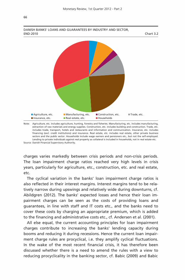
charges varies markedly between crisis periods and non-crisis periods. The loan impairment charge ratios reached very high levels in crisis years, particularly for agriculture, etc., construction, etc. and real estate, etc.

The cyclical variation in the banks' loan impairment charge ratios is also reflected in their interest margins. Interest margins tend to be rela-tively narrow during upswings and relatively wide during downturns, cf. Abildgren (2012). The banks' expected losses and hence their loan im-pairment charges can be seen as the costs of providing loans and guarantees, in line with staff and IT costs etc., and the banks need to cover these costs by charging an appropriate premium, which is added to the financing and administrative costs etc., cf. Andersen et al. (2001).

All else equal, the current accounting principles for loan impairment charges contribute to increasing the banks' lending capacity during booms and reducing it during recessions. Hence the current loan impair-ment charge rules are procyclical, i.e. they amplify cyclical fluctuations. In the wake of the most recent financial crisis, it has therefore been discussed whether there is a need to amend the rules with a view to reducing procyclicality in the banking sector, cf. Babic (2009) and Babic

DANISH BANKS' LOANS AND GUARANTEES BY INDUSTRY AND SECTOR, END-2010 Chart 3.2

Agriculture, etc. Manufacturing, etc. Construction, etc. Trade, etc.Insurance, etc. Real estate, etc. Households

Note: Source:

Agriculture, etc. includes agriculture, hunting, forestry and fisheries. Manufacturing, etc. includes manufacturing, extraction of raw materials and energy supplies. Construction, etc. includes building and construction. Trade, etc.includes trade, transport, hotels and restaurants and information and communication. Insurance, etc. includes financing (excl. credit institutions) and insurance. Real estate, etc. includes real estate, other private business sectors and the public sector. Households include wage earners and pensioners etc., but not the self-employed. Lending to private individuals against real property as collateral is included in households, not in real estate etc. Danish Financial Supervisory Authority.


67

DANISH BANKS' LOSSES AND LOAN IMPAIRMENT CHARGES ON LOANS AND GUARANTEES – BY INDUSTRY AND SECTOR Chart 3.3

-1

0

1

2

3

4

5

6

1992

1993

1994

1995

1996

1997

1998

1999

2000

2001

2002

2003

2004

2005

2006

2007

2008

2009

2010


Per cent Agriculture, etc.

0.0

0.2

0.4

0.6

0.8

1.0

1.2

1.4

1.6

1.8

2.0

1992

1993

1994

1995

1996

1997

1998

1999

2000

2001

2002

2003

2004

2005

2006

2007

2008

2009

2010


Per cent Manufacturing, etc.

0

2

4

6

8

10

12

1992

1993

1994

1995

1996

1997

1998

1999

2000

2001

2002

2003

2004

2005

2006

2007

2008

2009

2010


Per cent Construction, etc.

-0.5

0.0

0.5

1.0

1.5

2.0

2.5

3.0

1992

1993

1994

1995

1996

1997

1998

1999

2000

2001

2002

2003

2004

2005

2006

2007

2008

2009

2010


Per cent Trade, etc.

-0.5

0.0

0.5

1.0

1.5

2.0

1992

1993

1994

1995

1996

1997

1998

1999

2000

2001

2002

2003

2004

2005

2006

2007

2008

2009

2010


Per cent Insurance, etc.

0.0

0.5

1.0

1.5

2.0

2.5

3.0

3.5

4.0

4.5

5.0

1992

1993

1994

1995

1996

1997

1998

1999

2000

2001

2002

2003

2004

2005

2006

2007

2008

2009

2010


Per cent Real estate, etc.

-0.5

0.0

0.5

1.0

1.5

2.0

2.5

1992

1993

1994

1995

1996

1997

1998

1999

2000

2001

2002

2003

2004

2005

2006

2007

2008

2009

2010


Per cent Households

-0.5

0.0

0.5

1.0

1.5

2.0

2.5

3.0

1992

1993

1994

1995

1996

1997

1998

1999

2000

2001

2002

2003

2004

2005

2006

2007

2008

2009

2010


Per cent Total

Note: The aggregate loan impairment charge ratios have not been calculated but are based directly on the accounts statistics of the Danish Financial Supervisory Authority.


68

and Rasmussen (2010). One element of the debate has been the "Spanish model" for making provisions. This model entails that Spanish credit institutions must make loan impairment charges not only ac-cording to the principle of objective evidence of impairment ("specific provisions"), but also on the basis of average historical loss ratios over a business cycle ("dynamic provisions"). In periods with low specific pro-visions, the dynamic provisions are increased, while they are reduced in periods with high specific provisions. This means that a bank's total loan impairment charges in a given period become less cyclical, and in good times the bank builds up a buffer against losses in bad times.

In July 2009, the European Commission published its deliberations con-cerning implementation of dynamic provisions in accordance with the Spanish model as a supplement to loan impairment charges under the existing international accounting standards. In the European Commis-sion's consultation paper from February 2010, the thoughts about dynamic provisions had made way for contemplations about "counter-cyclical provisions" also aimed at ensuring that the banks, via loan im-pairment charges, build up buffers against their expected losses over a business cycle. The Commission has not followed up these proposals subsequently. So far, the regulatory response to the financial crisis in re-lation to the issue of procyclicality in the banking sector has mainly fo-cused on introducing countercyclical capital buffers, cf. Harmsen (2010) and Babic (2011).

Currently, the international accounting standards boards, IASB1 and FASB2, are working on proposals for new accounting standards to ensure that loan impairment charges are made at an earlier point than under the current principles. However, the proposals from the IASB and the FASB do not envisage smoothing of loan impairment charges over the business cycle.

4. LOAN IMPAIRMENT CHARGES AND MACRO STRESS TESTING OF THE BANKS' CAPITALISATION

Central banks and supervisory authorities have a number of different approaches to modelling loan impairment charges in connection with macro stress testing of the financial system, cf. e.g. Sorge (2004), Sorge and Virolainen (2006), Chan-Lau (2006), Foglia (2009) and Plesner (2012).

1 The International Accounting Standards Board, an independent organisation working to make

financial statements comparable across countries. 2 The Financial Accounting Standards Board, which develops accounting standards that are generally

accepted in the USA.


69

These approaches have different characteristics in terms of both degree of detail and methodology.

A basic distinction is often made between "top-down" and "bottom-up" stress testing. In top-down stress tests, the authorities perform all stress test calculations, while bottom-up stress tests are performed in cooperation with the banks whose resilience is to be tested. Conse-quently, in top-down stress tests, loan impairment charges are calculated using the authorities' macro stress testing models, while the calculations in bottom-up stress tests are based on the credit risk models of the indi-vidual banks.

This article focuses on models for calculation of the banks' loan impair-ment charges according to the top-down approach. Overall, the models can be divided into two groups: simultaneous models and satellite models. Simultaneous models This model type provides for simultaneous calculation of the macro-economic stress scenarios and the banks' loan impairment charges in the scenarios. This approach uses a simultaneous macroeconomic model that models not only macroeconomic variables such as economic growth, interest rates and house prices, but also both the banks' loan impair-ment charges (pass-through from the real economy to the banking sector) and the impact of the banks' lending capacity on the macro-economy (feedback effects from the banking sector to the real econ-omy), cf. Chart 4.1.

The simultaneous macroeconomic model may be a relatively small vector autoregressive (VAR) model or a larger structural macroeco-nometric model with relations describing the interaction between the banking system and the rest of the economy.

Small VAR models are relatively easy to maintain in step with eco-nomic developments, but since they are aggregated, their results could be difficult to interpret in depth in conformity with economic theory, cf. Abildgren (2012), Avouyi-Dovi et al. (2009) and Shahnazarian and Åsberg (2008).

OVERALL MODEL ARCHITECTURE – SIMULTANEOUS MODEL Chart 4.1

Real economy Banking sectorReal economy Banking sector


70

It requires far more resources to estimate and maintain large, structural macroeconometric models with a built-in financial sector. On the other hand, large structural models can make it easier to provide a description of the interaction between the financial and the real sectors which conforms to theory.

Given the relative complexity of simultaneous models, it may be neces-sary in practice to aggregate the modelling of the banking sector rather than modelling the profit and loss accounts and balance sheets of indi-vidual banks. This means that it is not possible to stress test the capital-isation of the individual banks – only the capitalisation of the banking system as a whole.

Satellite models Under this approach, various macroeconomic scenarios are constructed using a macroeconometric model, followed by modelling of the effects of the scenarios on the banks' loan impairment charges using a satellite model, cf. Borio et al. (2012). Danmarks Nationalbank applies the satel-lite approach in macro stress testing, and the relevant scenarios are constructed using Danmarks Nationalbank's macroeconometric model, MONA, cf. Danmarks Nationalbank (2003a, 2007a).

Typically, this stress testing approach implies construction of scenarios for both the expected economic development ("baseline scenario") and for hypothetical developments with adverse shocks to the economy ("stress scenarios"). The purpose of the scenarios is to throw light on the banks' resilience to possible, but not very probable, shocks to the econ-omy. The banks' capitalisation in the various scenarios is then calculated using a satellite model ("stress test model") with modules for calculation of the banks' loan impairment charges as well as their operating profit, etc. in the various scenarios, cf. Chart 4.2.

The strength of satellite models is their less complex model architec-ture, even in connection with a very detailed level of calculation based on modelling of the profit and loss accounts and balance sheets of indi-vidual banks. For example, in detailed satellite models, variations in the individual banks' exposures to different industries and sectors can be taken into account, which may be difficult in more aggregated models.

Modelling of loan impairment charges in satellite models There are a number of different approaches to modelling loan impair-ment charges in satellite models. Two main model types are examined in the following: macro factor models and accounts-based failure-rate models. In sections 5 and 6, these two model types are estimated on Danish data.


71

Macro factor models This model type is based on econometric relations that explain the banks' loan impairment charge ratios against the backdrop of develop-ments in a number of macroeconomic variables of importance to credit risk, according to generally accepted economic theory, cf. Bunn et al. (2005) and Haldane et al. (2007) for an example from the Bank of Eng-land.

Typical explanatory variables for the loan impairment charge ratio for corporate lending could be real economic growth, real interest rates, debt as a ratio of earnings, real prices of commercial properties, real unit labour costs, real commodity prices, etc. Examples of explanatory vari-ables for lending to households are unemployment, real income, real interest rates, debt as a ratio of income and real house prices.

As regards the level of aggregation, the modelling may relate to total loan impairment charges or loan impairment charges by industry or sector in the banking sector as a whole or for the individual banks.

Accounts-based failure-rate models Bernhardsen and Larsen (2007) and Bernhardsen and Syversten (2009) describe the use of an accounts-based failure-rate model for macro stress testing purposes at Norges Bank. In general, this approach implies con-structing a number of macroeconomic scenarios for the future economic development. Against this background, the development in each firm's financial ratios is projected in the various scenarios, followed by calcula-tion of each firm's probability of default and the banks' loan impair-ment charges. Carling et al. (2007) have estimated a similar model for

OVERALL MODEL ARCHITECTURE – SATELLITE MODEL Chart 4.2

Macro-economicscenarios

Market risk module

Operating profit module

Credit risk module

The banks’ excesscapital adequacy, etc. in the variousscenarios

Stress test model

Macro-economicscenarios

Market risk module

Operating profit module

Credit risk module

The banks’ excesscapital adequacy, etc. in the variousscenarios

Stress test model


72

Sweden. In addition to accounting variables, this model also includes macroeconomic variables in the description of the probability of default.

The strength of this model type is the detailed data material, which provides for very sophisticated examination of credit risk in the banks' lending portfolios. For example, it is possible to throw light on the banks' loan impairment charges broken down by the firms' industry, size, age, geographical location, etc.

On the other hand, accounts-based failure-rate models may contain variables that could be difficult to project to a satisfactory extent on the basis of macroeconomic indicators such as real GDP, e.g. auditors' quali-fications, cf. below.

5. MACRO FACTOR MODEL FOR DANISH BANKS' LOAN IMPAIRMENT CHARGES

This section estimates a macro factor model for Danish banks' loan impairment charge ratios by industry and sector. For each industry/sector the loan impairment charge ratio is modelled as a function of a number of macroeconomic variables. This enables calculation of loan impairment charge ratios by industry and sector in the projection period for each scenario in the stress test. Combining this information with the indi-vidual bank's credit exposures by industry and sector over the projection period makes it possible to calculate the individual bank's loan impair-ment charges for each scenario. The calculation of each bank's loan im-pairment charges in the scenarios can then allow for the distribution of each bank's credit exposures to households and various industries.1 But this model approach does not take into account any differences in the credit quality of the individual banks' loans and guarantees to a given industry.

Data The model is estimated on the basis of annual observations for the period 1992-2010. Observations for loan impairment charge ratios by industry and sector are described in section 3, while observations of the explanatory macroeconomic variables are from the MONA data bank.

1 The data constructed in section 3 for the banks' loan impairment charges by industry and sector

enables direct modelling of loan impairment charge ratios for the banks' loans and guarantees by industry and sector. The macro factor model defined in this section thus differs from the model described in Danmarks Nationalbank (2008, 2009a). Here, the banks' loan impairment charge ratios are estimated in two steps. The first step is to estimate a relation between loss ratios at industry/sector level and macroeconomic trends. The second step is to estimate a relation between the banks' aggregated loan impairment charge ratio relative to the loss ratios on the one hand and a set of macroeconomic variables on the other. Assuming that this relation is identical for all industries/sectors, it is possible to calculate the loan impairment charge ratios by industry/sector.


73

The explanatory macroeconomic variables are collected from the subset of MONA variables normally included in Danmarks Nationalbank's stress tests, cf. Appendix 1 in Stress tests, 2nd half 2011. Such limitation of the potential explanatory variables rules out the application of many variables that could be relevant in the modelling of loan impairment charge ratios (e.g. the debt levels of households and various industries or the prices of commercial or agricultural properties) since these vari-ables are not included in MONA. Moreover, the limitation implies that the potential explanatory variables are to be taken from among the relatively few aggregated "main variables" in Danmarks Nationalbank's stress tests and not from among the over 500 variables in MONA. The reason is that the detailed development in a number of specific vari-ables, such as agricultural exports, rent, etc., is not compiled separately in the stress scenarios.

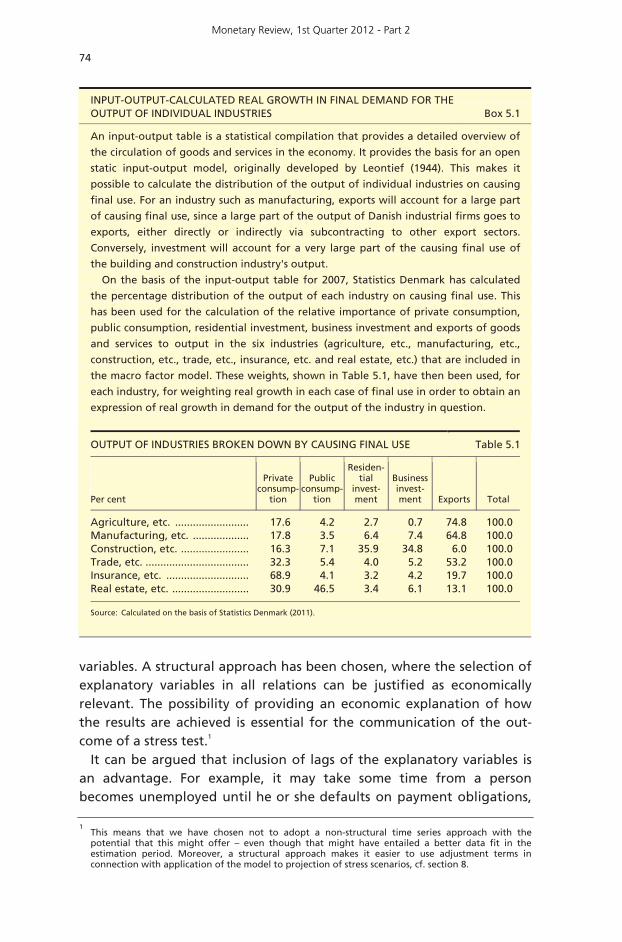
In general, MONA does not contain variables broken down by Indus-try, such as real growth in demand for the output of various industries, which should otherwise be regarded as more relevant to loan impair-ment charges on credit exposures by industry, compared with e.g. the development in total GDP. However, for each industry it is possible to obtain an expression of real growth in demand for that industry's out-put by weighting together real growth in private consumption, public consumption, residential investment, business investment and exports of goods and services using industry-specific weights based on input-output multipliers, cf. Box 5.1. As a result, the individual demand components are included with their direct or indirect impact on the output of the industry in question. Real growth in the demand for e.g. manufactured output that is directly or indirectly (via subcontractors) highly dependent on exports is thus given a high weight to real growth in exports, while real growth in demand for output from domestically oriented industries, such as building and construction, is given a high weight to real growth in investment.

Chart 5.1 shows the industry-specific expressions of real growth in de-mand for the output of the individual industries, while the other ex-planatory variables applied appear from Chart 5.2.1

Model specification For each industry and for households, the loan impairment charge ratio is modelled as a function of a number of explanatory macroeconomic

1 Besides the explanatory variables mentioned above, it has also been attempted to include real

growth in the export markets for manufactured output as a proxy of economic development abroad, given that non-residents are counterparties in around 40 per cent of Danish banks' lending to non-MFIs. However, since export market growth did not figure to any significant extent in the loan impairment charge relation for any industry, it has not been included in Chart 5.2.


74

variables. A structural approach has been chosen, where the selection of explanatory variables in all relations can be justified as economically relevant. The possibility of providing an economic explanation of how the results are achieved is essential for the communication of the out-come of a stress test.1

It can be argued that inclusion of lags of the explanatory variables is an advantage. For example, it may take some time from a person becomes unemployed until he or she defaults on payment obligations, 1 This means that we have chosen not to adopt a non-structural time series approach with the

potential that this might offer – even though that might have entailed a better data fit in the estimation period. Moreover, a structural approach makes it easier to use adjustment terms in connection with application of the model to projection of stress scenarios, cf. section 8.

INPUT-OUTPUT-CALCULATED REAL GROWTH IN FINAL DEMAND FOR THE OUTPUT OF INDIVIDUAL INDUSTRIES Box 5.1

An input-output table is a statistical compilation that provides a detailed overview of

the circulation of goods and services in the economy. It provides the basis for an open

static input-output model, originally developed by Leontief (1944). This makes it

possible to calculate the distribution of the output of individual industries on causing

final use. For an industry such as manufacturing, exports will account for a large part

of causing final use, since a large part of the output of Danish industrial firms goes to

exports, either directly or indirectly via subcontracting to other export sectors.

Conversely, investment will account for a very large part of the causing final use of

the building and construction industry's output.

On the basis of the input-output table for 2007, Statistics Denmark has calculated

the percentage distribution of the output of each industry on causing final use. This

has been used for the calculation of the relative importance of private consumption,

public consumption, residential investment, business investment and exports of goods

and services to output in the six industries (agriculture, etc., manufacturing, etc.,

construction, etc., trade, etc., insurance, etc. and real estate, etc.) that are included in

the macro factor model. These weights, shown in Table 5.1, have then been used, for

each industry, for weighting real growth in each case of final use in order to obtain an

expression of real growth in demand for the output of the industry in question.

OUTPUT OF INDUSTRIES BROKEN DOWN BY CAUSING FINAL USE Table 5.1

Per cent

Private

consump-tion

Public

consump-tion

Residen-tial

invest-ment

Business invest-ment

Exports

Total

Agriculture, etc. ......................... 17.6 4.2 2.7 0.7 74.8 100.0 Manufacturing, etc. ................... 17.8 3.5 6.4 7.4 64.8 100.0 Construction, etc. ....................... 16.3 7.1 35.9 34.8 6.0 100.0 Trade, etc. ................................... 32.3 5.4 4.0 5.2 53.2 100.0 Insurance, etc. ............................ 68.9 4.1 3.2 4.2 19.7 100.0 Real estate, etc. .......................... 30.9 46.5 3.4 6.1 13.1 100.0

Source: Calculated on the basis of Statistics Denmark (2011).


75

REAL GROWTH IN FINAL DEMAND FOR THE OUTPUT OF VARIOUS INDUSTRIES Chart 5.1

-14

-12

-10

-8

-6

-4

-2

0

2

4

6

8

10

12

14

1992

1993

1994

1995

1996

1997

1998

1999

2000

2001

2002

2003

2004

2005

2006

2007

2008

2009

2010

Agriculture, etc. Manufacturing, etc. Construction, etc.Trade, etc. Insurance, etc. Real estate, etc.

Per cent year-on-year

Source: See Box 5.1.

UNEMPLOYMENT, REAL GROWTH IN HOUSE PRICES AND SHORT-TERM AND LONG-TERM REAL INTEREST RATES Chart 5.2

Unemployment

0

2

4

6

8

10

12

1992

1993

1994

1995

1996

1997

1998

1999

2000

2001

2002

2003

2004

2005

2006

2007

2008

2009

2010

Per cent Real growth in house prices

-15

-10

-5

0

5

10

15

20

1992

1993

1994

1995

1996

1997

1998

1999

2000

2001

2002

2003

2004

2005

2006

2007

2008

2009

2010

Per cent year-on-year

Short-term real interest rate

-2

0

2

4

6

8

10

1992

1993

1994

1995

1996

1997

1998

1999

2000

2001

2002

2003

2004

2005

2006

2007

2008

2009

2010

Per cent p.a. Long-term real interest rate

-2

0

2

4

6

8

10

1992

1993

1994

1995

1996

1997

1998

1999

2000

2001

2002

2003

2004

2005

2006

2007

2008

2009

2010

Per cent p.a.

Source: MONA data bank.


76

when the loan impairment charges are made. One reason could be that the person in question has private means to use. But with only 19 annual observations, inclusion of one or two lags of just a few explanatory variables may soon give rise to problems with lack of degrees of freedom. Instead of including lags of the explanatory variables in the model, we have chosen to include the response variable (loan impairment charge ratio) as an explanatory variable with a lag of one year.1

The macro factor model is therefore specified as the following linear regression equations:

,eXbbNPSaNPS tj

k

nn,tnjjj,tjj,t ,

1,0,1

(5.1)

where NPSj,t is the loan impairment charge ratio in year t related to loans and guarantees to industry j, bj,0 is a constant term, X1,t ,…, Xk,t are explanatory variables2 and aj, bj,1, …, bj,k are parameters. Finally, ej,t are serially uncorrelated error terms with a mean value of zero and time-invariant variance.3

For the loan impairment charge ratio on loans and guarantees to households, the basic potential explanatory variables are the unemploy-ment rate, real interest rates and real growth in house prices. A priori, rising unemployment is expected to increase the loan impairment charge ratio since it reduces the households' ability to pay. Correspond-ingly, rising real interest rates are expected to increase the loan impair-ment charge ratio, since a higher level of interest rates increases the interest burden of the households. Conversely, rising real house prices are, all else equal, expected to reduce the loan impairment charge ratio since a considerable number of bank loans are based on real property as collateral.

1 This corresponds to the mindset behind the "Koyck lag", i.e. transforming an equation with an

infinite number of lags of the explanatory variables with geometrically declining coefficients into an equation including a one-period lag of the response variable as an explanatory variable together with the original explanatory variables without lags, cf. Koyck (1954) and Griliches (1967). Theoretically, the parameter of the autoregressive term in a Koyck lag will be between 0 and 1. An alternative approach to parsimonious modelling is panel data estimation with parameter restrictions across industries. Since our aim is the widest possible modelling of cross-industry variations in credit risk, this method has not been selected.

2 All explanatory variables are in real terms, e.g. real interest rates, real growth in house prices, etc.,

given the assumption that the debtor's income/ability to pay rises in step with inflation. 3 The model (5.1) can be perceived as an ARX model, i.e. an autoregressive (AR) model expanded to

include exogenous variables (X). The model (5.1) is estimated using the single-equation Ordinary Least Squares, OLS, method. Thus, any problems with endogeneity are disregarded. We have chosen a linear model specification which is easy to interpret. We have not chosen a logit approach since loan impairment charge ratios can be negative and hence outside the set interval between 0 and 1. Deterministic trends have not been used in the regression equations, because the estimated model is designed for stress scenario projection. In addition, all of the applied response and explanatory variables must be presumed to be stationary in a structural economic perspective.


77

For loan impairment charge ratios on loans and guarantees to the six industries, the basic potential explanatory variables are real growth in demand for the output of the industry, real interest rates and real growth in house prices. A priori, an increase in real growth in demand for the output of the industry is expected to reduce the loan impairment charge ratio, since higher turnover improves firms' ability to pay. Rising real interest rates are assumed to increase the loan impairment charge ratio, because a higher level of interest rates implies a larger interest burden for the firms. Conversely, rising real house prices are, all else equal, expected to reduce the loan impairment charge ratio, since a considerable number of bank loans are based on commercial properties as collateral, which normally display correlation with house prices, cf. Chart 5.3.

Estimation results Table 5.2 shows the estimated loan impairment charge relations. With a few exceptions, the individual relations include only the explanatory variables for which the parameter estimates differ significantly from zero.1 All of the estimated parameters have the expected signs, and

1 This choice was made in light of the modest number of degrees of freedom. In principle, the

exclusion of relevant explanatory variables may give rise to bias in the estimated parameter coefficients, but, as mentioned, only insignificant variables have been excluded.

PROPERTY PRICES Chart 5.3

30

40

50

60

70

80

90

100

110

120

13019

92

1993

1994

1995

1996

1997

1998

1999

2000

2001

2002

2003

2004

2005

2006

2007

2008

2009

2010

Single-family houses Commercial properties

2006 = 100

Note: Source:

Annual averages. Statistics Denmark.


78

there are no problems with autocorrelation in the relations at a signifi-cance level of 5 per cent. The high values of the determination coeffi-cient (R2) should be viewed in light of the use of smoothed loan impairment charge ratios, cf. Box 3.2.1

According to the estimated relation for loans and guarantees to households, an increase in unemployment by 3 percentage points will, all else equal, cause the loan impairment charge ratio to rise by 0.25 percentage point, while a drop in real house prices by 10 per cent will, all else equal, increase the loan impairment charge ratio by 0.5 percentage point. It should be noted, however, that the estimated coefficient of unemployment is not significantly different from zero, and that the unemployment rate has shown a clear downward trend since the early 1990s in step with the reduction of structural unemployment, cf. Andersen and Rasmussen (2011). In the estimation period 1992-2010 there have been no instances of a 3-percentage-point increase in unemployment from year to year. It is therefore uncertain whether the estimated effect on loan impairment charges from lending to house-holds will apply also in the event of a sharp increase in unemployment over a short period of time. This should be kept in mind if the relation is used for macro stress testing purposes, cf. also section 8 about model application.

In all of the estimated loan impairment relations for industries, real growth in demand for the industry's output is included as an explana-tory variable. For example, a 10-per-cent drop in real demand for the industry's output entails, all else equal, a rise of 1.5 percentage points in the loan impairment charge ratio, as regards loans and guarantees to construction, etc., Moreover, the development in real interest rates or real house prices has been found to have a significant effect on loan impairment charges for certain industries. For example, a 1-percentage-point increase in long-term real interest rates will, all else equal, cause the loan impairment charge ratio to rise by 0.2 percentage point as regards loans and guarantees to real estate, etc. When interpreting the relations for loan impairment charges on corporate lending, it should be borne in mind that both short-term and long-term real interest rates have shown a clear downward trend since the early 1990s. Consequent-ly, if there is a considerable increase in the level of interest rates, there is

1 If non-smoothed loan impairment charge ratios, described in Box 3.2, are used, almost the same

variables become significantly different from zero, with the same sign. R2 becomes somewhat lower, however, but the estimated loan impairment charge ratios do not differ to any noticeable extent from the ratios shown in Chart 5.4. Attempts have been made to include non-linear transformations of the explanatory variables (unemployment and interest rates) and asymmetrical treatment of increases and falls in house prices in alternative models. Inclusion of such terms did not result in better data fit.


79

a risk that the effect on loan impairment charges will differ from the effect that can be calculated directly on the basis of the relations.

Chart 5.4 compares actual and estimated loan impairment charge ratios. With the exception of manufacturing, etc. in the middle of the period, the actual and estimated loan impairment charge ratios are relatively closely related. This is also reflected in the relatively high deter-

ESTIMATED LOAN IMPAIRMENT RELATIONS Table 5.2

Response variable: Loan impairment charge ratio for loans and guarantees to

House-holds

Agricul-ture, etc.

Manufac-turing, etc.

Construc-tion, etc.

Trade, etc.

Insurance, etc.

Real estate, etc.

Explanatory variables:

Parameter estimate (standard error)

Constant .................. 0.0561 (0.193)

0.564***

(0.132) 0.401*** (0.135)

1.150*** (0.271)

0.430***

(0.0939) 0.467*** (0.0661)

0.692** (0.322)

Response variable, 1-year lag ................

0.355* (0.175)

0.601*** (0.0601)

0.608*** (0.143)

0.467*** (0.0720)

0.592***

(0.0784) 0.501*** (0.0805)

0.525*** (0.124)

Unemployment, per cent1 .........................

0.0829 (0.0494)

... ... ... ... ... ...

Real growth in house prices, per cent year-on-year ....................

-0.0484***

(0.0108) ... ... ... -0.0234*

(0.0128) ... ...

Short-term real interest rate, per cent p.a.2 ...........

... ... ... ... 0.0593* (0.0316)

... ...

Long-term real interest rate, per cent p.a.3 ...........

... ... ... ... ... ...

0.210** (0.0947)

Real growth in demand, per cent p.a.4 ..........................

...

-0.0917***

(0.0213)

-0.0447**

(0.0159)

-0.149***

(0.0338)

-0.0585**

(0.0266)

-0.144*** (0.0168)

-0.416*** (0.0833)

Number of observations ............ 18 18 18 18 18 18 18 R2 ............................. 0.842 0.887 0.676 0.847 0.929 0.905 0.817 Adjusted R25 ............ 0.808 0.872 0.633 0.826 0.907 0.893 0.778 AR(1)6 ....................... 0.452 0.975 0.896 0.248 0.142 0.0321 0.490 AR(1-2)6 .................... 2.345 1.001 1.418 0.324 0.0988 0.0215 0.442 JB7 ............................. 1.065 0.499 4.000 0.117 5.231* 0.639 2.058

1 Number of unemployed persons as a percentage of the labour force. 2 3-month collateralised money-market interest rate less year-on-year growth in the Harmonised Index of Consumer

prices, HICP. 3 Average bond yield less year-on-year growth in HICP. 4 Input-output-calculated real growth in final demand for the output of each industry, cf. Box 5.1. 5 Adjusted for the number of degrees of freedom. 6 LM test for autocorrelation (F form) with the order in brackets. The null hypothesis is no autocorrelation. 7 Jarque-Bera normality test with small sample adjustment. The null hypothesis is normality. Note: Estimated using the OLS method. * indicates rejection of the null hypothesis at a significance level of 10 per cent. ** indicates rejection of the null hypothesis at a significance level of 5 per cent. *** indicates rejection of the null hypothesis at a significance level of 1 per cent The null hypothesis on testing (double-sided) for significance of parameter estimates is that the parameter is equal

to zero. The delimitation of households and the individual industries is described in the note to Chart 3.2.


80

ACTUAL AND ESTIMATED LOAN IMPAIRMENT CHARGE RATIOS ON LOANS AND GUARANTEES FROM DANISH BANKS – MACRO FACTOR MODEL Chart 5.4

-1.0

0.0

1.0

2.0

3.0

4.0

5.0

1993

1994

1995

1996

1997

1998

1999

2000

2001

2002

2003

2004

2005

2006

2007

2008

2009

2010

Actual Estimated


0.0

0.2

0.4

0.6

0.8

1.0

1.2

1.4

1.6

1993

1994

1995

1996

1997

1998

1999

2000

2001

2002

2003

2004

2005

2006

2007

2008

2009

2010

Actual Estimated


-1

0

1

2

3

4

5

6

7

8

1993

1994

1995

1996

1997

1998

1999

2000

2001

2002

2003

2004

2005

2006

2007

2008

2009

2010

Actual Estimated


-1.0

-0.5

0.0

0.5

1.0

1.5

2.0

2.5

3.0

1993

1994

1995

1996

1997

1998

1999

2000

2001

2002

2003

2004

2005

2006

2007

2008

2009

2010

Actual Estimated


-0.5

0.0

0.5

1.0

1.5

2.0

2.5

1993

1994

1995

1996

1997

1998

1999

2000

2001

2002

2003

2004

2005

2006

2007

2008

2009

2010

Actual Estimated


-2

-1

0

1

2

3

4

5

1993

1994

1995

1996

1997

1998

1999

2000

2001

2002

2003

2004

2005

2006

2007

2008

2009

2010

Actual Estimated


-1.0

-0.5

0.0

0.5

1.0

1.5

2.0

2.5

1993

1994

1995

1996

1997

1998

1999

2000

2001

2002

2003

2004

2005

2006

2007

2008

2009

2010

Actual Estimated

Per cent Households

-1.0

-0.5

0.0

0.5

1.0

1.5

2.0

2.5

1993

1994

1995

1996

1997

1998

1999

2000

2001

2002

2003

2004

2005

2006

2007

2008

2009

2010

Actual Estimated

Per cent Total

Note: The estimated values of the total loan impairment charge ratio have been calculated by weighting loan impairment charge ratios by industry and sector using the weights of loans and guarantees. The actual total loanimpairment charge ratio has not been calculated, but is based directly on the accounts statistics of the DanishFinancial Supervisory Authority.


81

mination coefficients in Table 5.2. The estimated macro factor model is also able to explain the high levels of loan impairment charges during the crises in the early 1990s and the years from 2008 onwards. This is an important feature of models that are to be used for macro stress testing.

The calculations in Chart 5.4 are normally characterised as an "in-sample" test of the model, with the applied parameter estimates in all years being based on data for the entire period 1992-2010, and with actual lagged loan impairment charge ratios being applied in the calcu-lation of estimated loan impairment charge ratios. Since this is a very short data set that includes only few observations with a crisis in the banking sector, it makes no sense to perform a full "out-of-sample" test, calculating the parameter estimates on the basis of a subset of the observations in the data set. A partial out-of-sample test for the years 2007-09 – in which the parameter estimates are based on data for 1992-2010, but the estimated loan impairment charge ratios are used as lagged loan impairment charge ratios in the calculation of estimated loan impairment charge ratios in the projection period – results in an average absolute deviation from the actual loan impairment charge ratios in the three years of 0.3 percentage point for the sector as a whole. This corresponds to the average absolute prediction error in the in-sample test. The calculations thus illustrate that, also in a partial out-of-sample test, the model is able to generate high loan impairment charge ratios in a period of strong economic downturn.

6. ACCOUNTS-BASED FAILURE-RATE MODEL FOR THE LOAN IMPAIRMENT CHARGES OF DANISH BANKS

In this section, an accounts-based failure-rate model is estimated for Danish banks' loan impairment charge ratios for corporate credit expos-ures. In general, stress testing using this type of model implies construc-ting a number of macroeconomic scenarios for the future economic development. Against this background, the pattern of each firm's finan-cial ratios is projected in the various scenarios, followed by calculation of each firm's probability of default and the banks' loan impairment charges.

Data The data material behind the model consists of annual observations since 1995. Observations of the loan impairment charge ratios by Indus-try are described in section 3, while observations of the explanatory macroeconomic variables are from the MONA data bank and from the


82

subset of MONA variables included in Danmarks Nationalbank's stress test, cf. section 5.

The source of financial statements at micro level is a database consisting of the published financial statements of all Danish public and private limited liability companies with a balance-sheet total exceeding kr. 125.000, collected by Experian A/S. Credit institutions are excluded from the data set, since exposures vis-à-vis credit institutions are not included in the loans and guarantees that are the subject of the modelling of loan impairment charges. Moreover, a few special firms with large balance-sheet totals are excluded as they constitute only a limited risk to the banks. Cases in point are the Great Belt Bridge and Øresund Landworks as their debt is guaranteed by the government. Sole proprietorships are not comprised by the database. The data set consists of around 1,435,000 financial statements presented by around 96,000 firms on average for the financial years 1995-2009. The database also contains information about the number of failures and other firm-specific characteristics, such as age, geographical location, form of ownership, etc.

Estimation of the failure-rate model First, a modified version of Danmarks Nationalbank's failure-rate model is estimated.1 The model describes the probability of firm i failing2 in year t (PDi,t) on the basis of information on the firm's return on assets, debt, industry, geographical location, etc. in year t-2 (X1,i,t-2 ,…, Xk,i,t-2 ) as well as growth in real GDP in year t-1 (Z1,t-1).

3 This can be formally written as:

,ZaXbbFPD ,t

k

ntn,inti

111

12,0,

(6.1)

where b0 is a constant term, and b1, …, bk, a1 are parameters. The ex-planatory variables in the basic model are described in more detail in Table 6.1.

1 Danmarks Nationalbank's failure-rate model has not previously been used directly for macro stress

testing purposes. It is described in Danmarks Nationalbank (2003b, 2007b), Lykke et al. (2004) and Dyrberg (2004). The model estimated in this article contains the same variables as Danmarks Nationalbank's failure-rate model except for one variable indicating whether the financial statements of the firm in question have one or more auditors' qualifications. This variable has been excluded because it is difficult to project on the basis of macroeconomic variables.

2 Given the ultimate aim of modelling the banks' loan impairment charges, a broad-based definition

of "failure" is applied. A firm is regarded as having failed when one of the following events has occurred: (a) It is subject to compulsory liquidation or is being liquidated; (b) it has been or is being dissolved by the courts; (c) it is subject to a compulsory deed of arrangement with creditors or to a compulsory scheme of arrangement with creditors; or (d) it has been subject to enforced sale.

3 We have one comment in relation to the recording of failures in the data behind the equations

estimated in this section. All failures are placed two years after the end of the last year for which the firm presented financial statements as a going concern. The reason is that it, on average, takes 19 months from the presentation of the last financial statements as a going concern to the official affirmation of the compulsory liquidation, cf. Lykke et al. (2004).


83

EXPLANATORY VARIABLES IN (6.1) Table 6.1

Explanatory variables

Expected effect on probability

of default

Description

Firm-specific variables (included with a 2-year lag): Return on assets ......... - The firm's return on assets less the median return

on assets for the relevant industry. The return on assets is calculated as the profit for the year before interest (primary operating result) as a ratio of total assets at year-end.

Debt ratio (short-term) ................

+ Short-term debt as a ratio of the balance-sheettotal, year-end.

Debt ratio (long-term) .................

+ Long-term debt as a ratio of the balance-sheettotal, year-end.

Size ............................. - The logarithm of the balance-sheet total in kr. 1,000 at year-end deflated by the GDP deflator (1995 = 1).

Eroded capital base .... + The dummy variable is set at 1 if the firm has made a loss over the last year, and if another loss will mean that the firm's equity capital falls below the statutory requirement for capital size in new companies. Otherwise, the dummy vari-able is set at 0.

Form of ownership .... + The dummy variable is set at 1 if the firm is a private limited liability company (ApS) at year-end. Public limited liability companies (A/S) con-stitute the reference group (with the value 0). The statutory capital requirement for establish-ment of public limited liability companies is higher than for private limited liability com-panies.

Age - Dummy variables representing the firm's age at year-end measured as the number of full years. Newly established firms aged less than 1 year constitute the reference group (with the value 0).

Industry ...................... +/- Dummy variables for each industry. They are to capture industry-specific differences in the level of probability of default.

Municipality group .... - Dummy variables indicating the firms' domiciles at year-end by municipality group, with Greater Copenhagen as the reference group (with the value 0). Greater Copenhagen is normally more sensitive to cyclical fluctuations than the prov-inces.

Macroeconomic variables (included with a 1-year lag): Real GDP growth ....... - Year-on-year growth in real GDP. This variable is

to capture general cyclical developments.


84

ESTIMATION OF FAILURE-RATE MODEL (6.1) Table 6.2

Coefficient estimate

Standard error

Change in odds ratio

when explanatory variable changes by

one unit

Constant .................................................... -1.271*** 0.0391 ... Return on assets, percentage points ....... -0.00148*** 0.000111 0.999 Debt (short-term), ratio ............................ 0.267*** 0.00714 1.306 Debt (long-term), ratio ............................. 0.0427*** 0.0127 1.044 Size, log 1000 1995-kr. ............................. -0.310*** 0.00404 0.733 Form of ownership, dummy (1=private;0=public) ................................................... 0.238*** 0.0151 1.268 Eroded capital base, dummy (1=YES; 0=NO) ........................................... 1.121

***

0.0116

3.097

Real GDP growth, per cent p.a. ............... -0.0937*** 0.00172 0.911

Note: The explanatory variables are described in Table 6.1. The response variable in the estimated equation is the logarithm of the "odds ratio", i.e. the probability of "failing" divided by the probability of "continuing as a goingconcern". The figures in the column "change in odds ratio when explanatory variable changes by one unit" arethe antilogarithms of the figures in the column of coefficient estimates.

Besides the variables shown in the table, the estimated model contains dummy variables for industry, municipalitygroup and age.

* indicates that a coefficient is significantly different from zero at a significance level of 10 per cent. ** indicates that a coefficient is significantly different from zero at a significance level of 5 per cent. *** indicates that a coefficient is significantly different from zero at a significance level of 1 per cent.

In purely econometric terms, the basic model in equation (6.1) is esti-mated as a logistic regression model1, and the result is shown in Table 6.2. The response variable is the logarithm of the odds ratio, i.e. the probability of "failing" relative to the probability of "continuing as a going concern". This is a "relative risk of default", in the following referred to as "probability of default".

In light of the large number of observations, it can be argued that the coefficient estimates should be assessed at a lower significance level than the customary 5 per cent. All of the estimated coefficients in the basic model differ significantly from zero at a significance level of 1 per cent and have the expected signs, cf. also Table 6.1. For example, it is seen that the higher the firm's return on assets and the lower its debt, the lower its default risk.

Since the estimated failure-rate model is a non-linear model, and since the response variable is the logarithm of the odds ratio, the inter-pretation of the estimated coefficients is not as simple as in a linear re-gression model. Consequently, Table 6.2 also contains a column showing the change in the odds ratio on a one-unit change in the explanatory

1 The model is estimated with maximum likelihood. The estimation rests on a multinomial logistic

regression model with 4 outcomes ("going concern", "failure", "voluntary closure" and "merger"). The baseline outcome in the model is "going concern". The estimation approach is based on the assumption that the large number of dummy variables is sufficient to control for heterogeneity across firms. An alternative approach would have been a panel data approach, whereby the estimation could take unobservable heterogeneity across firms into account.


85

variable. For instance, it could be deduced from Table 6.2 that, all else equal, the default risk is approximately three times higher for a firm with an eroded capital base than for a similar firm whose capital base is not eroded. The probability of default is around 27 per cent higher for a private limited liability company (ApS) than for a similar firm organised as a public limited liability company (A/S). Estimation of relations between corporate financial statements and macroeconomic variables In order to estimate the probabilities of default of firms in a future stress testing cycle, it is necessary to construct models for projection of the accounting variables included in the failure-rate model. Danmarks Nationalbank's stress tests are based on a 3-year stress testing cycle, which requires projection of accounting variables by up to 3 years.

Models are constructed with a view to projection of firms' size, short-term and long-term debt ratios, earnings and equity capital. The project-tions of a firm's earnings and equity capital are necessary in order to determine whether the capital base is eroded. As regards the other firm-specific variables in the failure-rate model (return on assets, form of ownership, age, industry and municipal group), no actual projection is made since the values are just carried forward unchanged. In principle, the age variable should be increased in the projection period, but since the population of firms is constant in the projection period, firm age is also kept constant.1

Accounting variables are modelled for 60 different groups of firms defined on the basis of form of ownership, industry and geographical location. If Y denotes the accounting variable to be projected, g the group, i the firm and t the year, the basic model can be written as fol-lows:

,eZaXbbY tig

m

nn,tigng

k

ntnnggtg,i ,,

1,,,

1,,0,,

(6.2)

where bg,0 is a constant term, and bg,1, …, bg,k and ag,1, …, ag,m are parameters. X1,t, …, Xk,t are macroeconomic variables, while Zg,i,1,t, …, Zg,i,m,t are firm-specific characteristics. Finally, eg,i,t are serially uncorrelated error terms with a mean value of zero and time-invariant variance. The

1 The reason is that the combination of increasing firm age and maintaining a constant population

would otherwise lead to underestimation of probabilities of default, since a firm's probability of default declines as it ages, all else equal. We have chosen to keep population and age constant in the projection period as a resource-saving alternative to actual simulation of new firms and failures in the projection period.


86

macroeconomic variables should be selected on the basis of the variables included in Danmarks Nationalbank's stress tests. As regards firm-specific characteristics, the dummy variables for age are included in all model specifications in order to "eliminate" the age effect. In add-ition, the variable for return on assets is included where it is found to have an effect on the development in the accounting variable. The 10 per cent highest and lowest observations for each group are excluded in order to minimise the effect of outliers at firm level in the estima-tions.

The projection of firm size is based on nominal balance-sheet growth, modelled as a function of nominal GDP growth and the dummy vari-ables for age. Nominal GDP growth is expected to produce a positive parameter estimate as nominal balance-sheet totals – like GDP – tend to increase in step with price developments. Moreover, higher economic ac-tivity tends to boost the firms' balance-sheet totals via reinvested earn-ings. Finally, high activity generates a need for a larger capital stock and thus expansion of balance-sheet totals.

An aggregate model is constructed for projection of the change in the sum of short-term and long-term debt ratios. Besides the dummy vari-ables for age, this model includes three macroeconomic variables. The first variable is defined as the difference between the real bond yield in the current year and the average real bond yield in the period 1980-2010. According to a study by Bancel and Mittoo (2004), more than 40 per cent of the firms in the survey indicate that low interest rates play an important role in their decisions on debt issuance. A negative param-eter estimate is thus expected for this variable. The second macroeco-nomic variable is real GDP growth. Higher real GDP growth is expected to have a positive impact on firms' balance-sheet totals, entailing a lower debt ratio. If the profit is spent on repayment of debt instead of boosting the balance-sheet total, the debt ratio will also fall. A negative parameter estimate is thus expected for this variable. The third and last variable is real growth in corporate building and construction invest-ment. Rising building and construction investment will have a positive impact on balance-sheets totals, but since such investment tends to be debt financed, this will have an even stronger upward effect on debt in relative terms. A positive parameter estimate is thus expected for this variable.

The models for projection of firms' earnings and equity capital have identical specifications. The change in firms' earnings or equity capital relative to the balance-sheet total is estimated as a function of the change in real GDP growth, the variable for return on assets and the dummy variables for age. Acceleration of real GDP growth is expected to


87

boost balance-sheet totals, but, given the hypothesis that both earnings and equity capital will increase relatively more, a positive parameter estimate for the change in real GDP growth is expected.

Table 6.2 shows descriptive statistics for the parameter estimates of the four accounting variables for the 60 groups of firms. Consequently, this is a highly condensed table, summarising the results of 60 regression equations. It is seen that the signs of the estimated parameters are as expected in most cases. However, in a number of cases the parameter estimates of corporate building and construction investment are contrary to expectations in the models for firms' debt ratios. This should be viewed in light of the substantial correlation between the explanatory variables, which makes it difficult to distinguish between the effects of the individual explanatory variables since the variables partially contain the same information. For example, corporate building and construction investment is included as part of GDP. Table 6.3 in-cludes the parameter estimates with the signs and values obtained on estimation of the models. However, when applying the models, the par-ameter estimates are set at 0 in the cases where the sign is contrary to expectations.

DESCRIPTIVE STATISTICS FOR PARAMETER ESTIMATES IN THE PROJECTION RELATIONS FOR THE 60 GROUPS Table 6.3

Response variable:

Nominal balance-

sheet growth, per cent year-on-

year

Change in debt ratio, percentage points

Change in profit/balance–sheet

total, percentage

points

Change in equity

capital/balance-sheet

total, percentage

points

Explanatory variable:

Nominal growth in GDP, year-

on-year

Real bond yield for the year less the average for 1980-2010, percentage

points

Real growth in GDP, per cent year-on-year

Real growth in building and con-struction

investment, per cent year-on-

year

Change in real growth

in GDP, percentage

points

Change in real

growth in GDP,

percentage points

Average parameter estimate .................................... 1.026 -0.366 -0.128 0.005 0.614 0.187 Standard deviation .............. 0.287 0.165 0.118 0.030 0.208 0.103 Minimum.............................. 0.296 -1.005 -0.663 -0.068 -0.115 -0.074 Maximum ............................. 1.678 0.095 0.177 0.172 1.009 0.586 Number of expected signs ... 60 57 54 36 58 58 Number of unexpected signs .....................................

0

3

6

24

2

2

Note: Descriptive statistics for parameter estimates on estimation of equation 6.2 using the pooled OLS method for the60 groups of firms defined on the basis of form of ownership, industry and geographical location.


88

In the model for nominal balance-sheet growth, the average parameter estimate for nominal GDP growth is 1.026. This should be taken to mean that an increase in nominal GDP of 1 per cent will, all else equal, entail an increase in the nominal balance-sheet total of 1.026 per cent for a firm in an average group. Estimation of debt-weighted probabilities of default It is possible to calculate the overall probability of default in an industry using the estimated failure-rate model. This is done by weighting the probability of default for each firm with its total debt relative to total debt in the industry.1 This can be formally written as:

,DD

PDPDji tj

titij,t

,

,, (6.3)

where PD denotes the probability of default, j the industry, t the year, i the firm and D the debt.

The industry-specific debt-weighted probabilities of default rose in connection with the economic downturn in 2001-03 and the financial crisis in 2009-10, cf. Chart 6.1. In the chart, debt-weighted probabilities of default have been calculated on the basis of both actual and pro-jected accounts data constructed by extending the previously mentioned projection relations up to 3 years into the future. A 3-year horizon cor-responds to the projection period used in Danmarks Nationalbank's stress tests. This throws light on the extra element of uncertainty introduced by using the failure-rate model rather than the macro factor model for macro stress testing. The extra element of uncertainty in the use of the failure-rate model for stress testing occurs because it is necessary to pro-ject not only macroeconomic developments, but also the financial state-ments of the individual firms.

It is seen that there are only minor differences between the debt-weighted probabilities of default calculated on the basis of actual and projected accounts data, respectively. This can be attributed partly to the explanatory power of the relations for projection of the accounting variables, partly to the importance of GDP growth as an explanatory variable in the failure-rate model.

1 Danish firms are not obliged to specify bank debt in their financial statements, so total debt is used

in the weighting.


89

Estimation of relations between loan impairment charge ratios and debt-weighted probabilities of default For each industry, a relation is then modelled between the loan impair-ment charge ratio and the debt-weighted probabilities of default calcu-lated using the failure-rate model. The two variables generally show positive correlation, cf. Chart 6.2, but with some differences. One underlying factor is that the data material behind the debt-weighted probabilities of default does not, as mentioned previously, comprise Danish sole proprietorships or non-resident firms. Moreover, the debt-weighted probabilities of default are based on weighting the probabilities of default for the individual firms with their total debt and not just their

DEBT-WEIGHTED PROBABILITIES OF DEFAULT Chart 6.1

0.0

0.5

1.0

1.5

2.0

2.5

1997

1998

1999

2000

2001

2002

2003

2004

2005

2006

2007

2008

2009

2010

2011

Actual accounts data Projected 1 yearProjected 2 years Projected 3 years


0.0

0.2

0.4

0.6

0.8

1997

1998

1999

2000

2001

2002

2003

2004

2005

2006

2007

2008

2009

2010

2011



0.0

0.5

1.0

1.5

2.0

2.5

3.0

1997

1998

1999

2000

2001

2002

2003

2004

2005

2006

2007

2008

2009

2010

2011



0.0

0.3

0.6

0.9

1.2

1.5

1997

1998

1999

2000

2001

2002

2003

2004

2005

2006

2007

2008

2009

2010

2011



0.0

0.2

0.4

0.6

0.8

1997

1998

1999

2000

2001

2002

2003

2004

2005

2006

2007

2008

2009

2010

2011



0.0

0.5

1.0

1.5

2.0

2.5

1997

1998

1999

2000

2001

2002

2003

2004

2005

2006

2007

2008

2009

2010

2011




90

debt to Danish banks. Finally, the loan impairment charge ratios reflect that the banks have a certain amount of collateral for the credits granted. In addition, the banks may, in certain cases, choose to make voluntary loan impairment charges on a corporate exposure simply to prevent the firm from failing.

Only 15 annual observations entail a very limited number of degrees of freedom and a need for parsimonious modelling. The point of departure is the mindset behind the traditional theory of credit risk modelling, cf. Bluhm et al. (2010). Here, the expected loss on a loan

DANISH BANKS' LOAN IMPAIRMENT CHARGE RATIOS AND DEBT-WEIGHTED PROBABILITIES OF DEFAULT Chart 6.2

-1.0

-0.5

0.0

0.5

1.0

1.5

2.0

2.5

3.0

1996

1997

1998

1999

2000

2001

2002

2003

2004

2005

2006

2007

2008

2009

2010

Loan impairment charge ratio Debt-weighted probability of default


0.0

0.2

0.4

0.6

0.8

1.0

1.2

1.4

1.6

1996

1997

1998

1999

2000

2001

2002

2003

2004

2005

2006

2007

2008

2009

2010



0.0

1.0

2.0

3.0

4.0

5.0

6.0

1996

1997

1998

1999

2000

2001

2002

2003

2004

2005

2006

2007

2008

2009

2010



-0.5

0.0

0.5

1.0

1.5

2.0

1996

1997

1998

1999

2000

2001

2002

2003

2004

2005

2006

2007

2008

2009

2010



-0.5

0.0

0.5

1.0

1.5

2.0

1996

1997

1998

1999

2000

2001

2002

2003

2004

2005

2006

2007

2008

2009

2010

Loan impairment charge ratiio Debt-weighted probability of default


0.0

0.5

1.0

1.5

2.0

2.5

3.0

3.5

1996

1997

1998

1999

2000

2001

2002

2003

2004

2005

2006

2007

2008

2009

2010

Loan impairment charage ratio Debt-weighted probability of default


Note: Debt-weighted probabilities of default with a 1-year lead, i.e. the probability of default shown for 2010 refers to

2011.


91

portfolio (EL) is often regarded as a product of the expected exposure at default (E[EAD]), the expected loss given default (E[LGD]) and the probability of default (PD)1:

PD,LGDEEADEEL (6.2)

or:

,PDLGDEEADEEL

(6.3)

where EL/E[EAD] is the expected loss ratio. Hence, the expected loss ratio depends on the probability of default and the expected loss given de-fault. The latter is determined by many factors, including the extent of collateralisation and ranking the event of liquidation.

With inspiration from the above, the following relation is specified for each sector:

,eRPHbPDbbNPSaNPS tjtjj,tjjj,tjj,t ,2,11,0,1 (6.4)

where NPSj,t is the loan impairment charge ratio in year t on loans and guarantees to industry j, PDj,t+1 is the debt-weighted probability of default in year t+1 in industry j, and ej,t are serially uncorrelated error terms with the mean value of zero and time-invariant variance. The debt-weighted probability of default is subject to a 1-year lead in the specification since loan impairment charges are booked before losses, cf. Chart 3.1. Moreover, bj,0 are industry-specific constant terms, and RPHt is real growth in house prices in year t. Real growth in house prices can be seen as a proxy for real growth in prices for commercial properties.

A priori, a rise in the probability of default for industry j should be expected to increase loan impairment charges on loans and guarantees to industry j. On the other hand, a rise in real house prices should, all else equal, be expected to reduce the loan impairment charge ratio,

1 This simple relation assumes that EAD, LGD and PD are independent, which is not always the case,

however. For instance, assume that PD increases in a recession. In that event, a bank may have to divest collateral (e.g. real estate) acquired from the liquidation estate of a customer, which may contribute to downward pressure on prices in the property market. This causes LGD to rise. Or assume that firms draw fully on their credit lines in a recession with rising PD. This results in a higher EAD for the bank.


92

since rising house prices increase the value of the collateral pledged for the credit granted.1

Table 6.4 shows the estimated relations. All of the estimated slope parameters have the expected sign, and most of them differ significantly from zero.

Chart 6.3 shows actual and estimated loan impairment charge ratios. The estimated model is generally able to explain developments in the

1 The relations are estimated using the single-equation OLS method. This method disregards any

problems with endogeneity, which could arise e.g. if high loan impairment charge ratios in the banking sector lead to fire sale of properties, resulting in falling property prices. In light of the limited number of degrees of freedom, an alternative approach could have been selected, based on panel data estimation with cross-industry parameter restrictions. However, this method was not chosen since we aimed at modelling cross-industry differences in the relations to the largest possible extent.

ESTIMATED RELATIONS BETWEEN LOAN IMPAIRMENT CHARGE RATIOS AND PROBABILITIES OF DEFAULT Table 6.4

Response variable: Loan impairment charge ratio for loans and guarantees to

Agriculture, etc.


Construc-tion, etc.

Trade, etc.

Insurance, etc.

Real estate, etc.

Explanatory variables:

Parameter estimate (standard error)

Constant .................... -0.771 (0.710)

0.0534 (0.489)

-1.523** (0.558)

-0.386 (0.508)

-0.589*** (0.172)

-0.428 (0.321)

Response variable, 1-year lag ..................

0.732*** (0.155)

0.540*** (0.158)

0.686*** (0.0948)

0.565*** (0.122)

0.357*** (0.0809)

0.489*** (0.0972)

Probability of default, 1-year lead ................

1.005 (0.603)

0.822 (1.142)

1.791*** (0.414)

1.049 (0.648)

3.074*** (0.529)

1.079*** (0.294)

Real growth in house prices, per cent year-on-year ......................

-0.0168 (0.0229)

-0.0268** (0.0116)

-0.0241 (0.0212)

-0.0227 (0.0148)

-0.0172** (0.00724)

-0.0387** (0.0128)

Number of observations .............. 15 15 15 15 15 15 R2 .............................. 0.801 0.767 0.960 0.866 0.953 0.914 Adjusted R21 .............. 0.747 0.704 0.949 0.830 0.940 0.891 AR(1)2 ......................... 1.102 0.0597 4.237* 1.054 0.576 0.00453 AR(1-2)2 ...................... 1.989 3.744* 2.234 1.085 0.281 0.597 JB3 .............................. 3.717 2.124 0.0466 0.126 0.343 0.426

1 Adjusted for the number of degrees of freedom. 2 LM test for autocorrelation (F form). The null hypothesis is no autocorrelation. 3 Jarque-Bera normality test with small-sample adjustment. The null hypothesis is normality. Note: Estimated using the OLS method. Endogeneity problems, if any, are disregarded, but they are, however, limited by

the loan impairment charge ratio with a lead being based on lagged accounts data to a large extent. * indicates rejection of the null hypothesis at a significance level of 10 per cent. ** indicates rejection of the null hypothesis at a significance level of 5 per cent. *** indicates rejection of the null hypothesis at a significance level of 1 per cent The null hypothesis on testing (double-sided) for significance of parameter estimates is that the parameter is equal

to zero. The delimitation of the individual industries is described in the note to Chart 3.2.


93

loan impairment charge ratios, including the substantial increase in con-nection with the financial crisis.

7. COMPARISON OF THE MODELS FOR LOAN IMPAIRMENT CHARGES

Table 7.1 and Chart 7.1 compare the actual loan impairment charge ratios for the six industries with the estimated loan impairment charge ratios from the macro factor model from section 5 and the accounts-based failure-rate model from section 6.

ACTUAL AND ESTIMATED LOAN IMPAIRMENT CHARGE RATIOS ON LOANS AND GUARANTEES FROM DANISH BANKS – FAILURE-RATE MODEL Chart 6.3

-0.5

0.0

0.5

1.0

1.5

2.0

2.5

1997

1998

1999

2000

2001

2002

2003

2004

2005

2006

2007

2008

2009

2010

Actual Estimated

Agriculture, etc.

-0.5

0.0

0.5

1.0

1.5

1997

1998

1999

2000

2001

2002

2003

2004

2005

2006

2007

2008

2009

2010

Actual Estimated

Manufacturing, etc.

-1.0

0.0

1.0

2.0

3.0

4.0

5.0

6.0

1997

1998

1999

2000

2001

2002

2003

2004

2005

2006

2007

2008

2009

2010

Actual Estimated

Construction, etc.

-1.0

-0.5

0.0

0.5

1.0

1.5

2.0

1997

1998

1999

2000

2001

2002

2003

2004

2005

2006

2007

2008

2009

2010

Actual Estimated

Trade, etc.

-0.5

0.0

0.5

1.0

1.5

2.0

2.5

1997

1998

1999

2000

2001

2002

2003

2004

2005

2006

2007

2008

2009

2010

Actual Estimated

Insurance, etc.

-1.0

0.0

1.0

2.0

3.0

4.0

1997

1998

1999

2000

2001

2002

2003

2004

2005

2006

2007

2008

2009

2010

Actual Estimated

Real estate, etc.

Note: The estimated loan impairment charge ratios are calculated on the basis of accounts data projected 1 year.


94

ACTUAL AND ESTIMATED LOAN IMPAIRMENT CHARGE RATIOS ON LOANS AND GUARANTEES FROM DANISH BANKS – COMPARISON OF MODELS Chart 7.1

-0.5

0.0

0.5

1.0

1.5

2.0

2.5

1997

1998

1999

2000

2001

2002

2003

2004

2005

2006

2007

2008

2009

2010

Actual Estimated - macro factor model Estimated - failure-rate model


-0.5

0.0

0.5

1.0

1.5

1997

1998

1999

2000

2001

2002

2003

2004

2005

2006

2007

2008

2009

2010



-1

0

1

2

3

4

5

6

1997

1998

1999

2000

2001

2002

2003

2004

2005

2006

2007

2008

2009

2010



-1.0

-0.5

0.0

0.5

1.0

1.5

2.0

1997

1998

1999

2000

2001

2002

2003

2004

2005

2006

2007

2008

2009

2010



-0.5

0.0

0.5

1.0

1.5

2.0

2.5

1997

1998

1999

2000

2001

2002

2003

2004

2005

2006

2007

2008

2009

2010



-1.0

0.0

1.0

2.0

3.0

4.0

1997

1998

1999

2000

2001

2002

2003

2004

2005

2006

2007

2008

2009

2010



DEVIATION BETWEEN ACTUAL AND ESTIMATED LOAN IMPAIRMENT CHARGE RATIOS 1997-2010 Table 7.1

Percentage points

Agricul-ture, etc.


Construc-tion, etc.

Trade, etc.

Insurance, etc.

Real estate, etc.

Average absolute deviation Macro factor model .......... 0.3 0.2 0.5 0.2 0.1 0.4 Failure-rate model ............ 0.3 0.2 0.3 0.2 0.1 0.3

Mean square error (MSE) Macro factor model .......... 0.1 0.1 0.4 0.0 0.0 0.2 Failure-rate model ............ 0.1 0.0 0.2 0.1 0.0 0.1

Average deviation Macro factor model .......... 0.0 0.0 0.0 0.0 0.0 0.0 Failure-rate model ............ 0.0 0.0 0.1 0.0 0.0 0.0


95

Both models provide a good description of the historical patterns of loan impairment charges and are able to explain the high levels of loan impairment charges during the crisis in the years from 2008 onwards. As mentioned previously, this is an important feature of models that are to be used for macro stress testing.

8. MODEL APPLICATION AND ADJUSTMENT TERMS

By definition, all models are simplified presentations of reality. So when constructing model-based projections, it is customary to include extra information besides that contained in the model's estimated relations. The extra information is implemented by means of adjustment terms, cf. Christensen (1978).

A model can be seen as an instrument for making projections in dia-logue with its user. This also applies to models for banks' loan impair-ment charges. Models help the user to ensure consistency in the analyses performed and may provide inspiration for disseminating the "stories" contained in the scenarios.

It is also customary to work with a range of models based on different approaches. Applying different types of models for the banks' loan im-pairment charges provides a more robust picture of the risks associated with the various stress scenarios. Different models may have different strengths and provide different opportunities for illustrating the re-spective scenarios in terms of coverage, degree of detail, etc. For ex-ample, the failure-rate model provides a basis for gaining a very detailed overview of developments in probabilities of default over the projection period, broken down by, say, sub-sectors and corporate debt levels. This makes it easier to incorporate extra information for macro stress testing of the financial system.

It is necessary to add a few specific comments as regards application of the models for loan impairment charges estimated in sections 5 and 6 for stress testing.

As mentioned in section 5, the period 1992-2010 – which has been used for estimation of the macro factor model – is characterised by a clear downward trend in both unemployment and short-term and long-term interest rates. It is therefore uncertain whether the models' parameter estimates can be assumed to apply to periods of sharp increases in unemployment and interest rates over a short period of time. Similar issues apply to the accounts-based failure-rate model, which has been estimated on the basis of an even shorter data period than the macro factor model.

Moreover, the models in sections 5 and 6 do not take into account any differences in the credit quality of the individual banks' loans and guar-


96

antees to a given industry. This may also entail a need for adjustment terms for some banks.

One way to take into account differences in credit quality could be to take the bank-specific data for total loan impairment charges and loans and guarantees broken down by industry/sector reported to the Danish Financial Supervisory Authority as the point of departure. On the basis of the banking sector's aggregate loan impairment charge ratios by industry and sector, shown in Box 3.2, and the bank-specific exposures, it is possible to calculate the total loan impairment charges that each bank would have made if its loan impairment charge ratio had matched that of the sector overall. If a given bank has systematically had higher actual loan impairment charge ratios than those that can be calculated on the basis of the banking sector's aggregate loan impairment charge ratios by industry and sector, this could indicate that the loans granted by the bank in question involve relatively high credit risk. In addition, it could be investigated whether lending and funding rates can be applied as indicators of the credit quality of a bank's loan portfolio. An advantage of interest-rate indicators is that they are more forward-oriented than historical loan impairment charges.

As regards the failure-rate model, the database provides information about the firm's main bank for around half of the firms included, cf. Abildgren et al. (2011). If the firms that have stated their main bank can be assumed to be representative of the loan portfolios of the individual banks, this will provide a basis for including bank-specific differences in terms of the credit quality of loans and guarantees in the loan impair-ment charges calculated using the failure-rate model.

During the most recent financial crisis, the Danish government has implemented extensive support measures, e.g. Bank Rescue Package 1 (general government guarantee for the banks' depositors and unsecured creditors) in October 2008, and Bank Rescue Package 2 (government capital injections into banks and the option to purchase individual gov-ernment guarantees for non-subordinated unsecured debt) in February 2009. Without these initiatives, the economic crisis would undoubtedly have been worse, and the banks' loan impairment charges would have been larger than they actually were. This should be borne in mind if the models are to be used for simulating loan impairment charges in stress scenarios without such massive government support.

Furthermore, it should be noted that any feedback effects from a stressed banking sector to the macroeconomy must, to some extent, be treated separately outside the models constructed using the satellite approach. Actual historical loan impairment charge ratios used for esti-mating the models reflect the historical feedback effects seen in con-


97

nection with banking crises. If the stress scenarios analysed involve macroeconomic developments that are worse than those seen during the banking crises occurring in the estimation period, it may be necessary to incorporate further feedback effects outside the models. For example, this could be the case in the event of a non-linear relation between the extent of a banking crisis and its feedback effects on the real economy.

It is also possible that the effects of banking crises on loan impairment charges depend on the frequency of such banking crises. For example, if one banking crisis follows immediately after another, the impact on loan impairment charges may be greater than if the banking crises are 15-20 years apart. The reason is that households and firms have little time to consolidate if one financial crisis is succeeded by another.

Finally, it should be mentioned that although there are many simi-larities between financial crises, they also differ. To the extent that a stress scenario includes new risk factors not reflected in historical events, it may be necessary to adjust the results calculated using loan impair-ment charge models estimated on the basis of historical data.

9. CONCLUDING REMARKS

The period since the mid-1990s has been characterised by increased focus on financial stability among central banks worldwide. In 1996, the Bank of England began to publish regular Financial Stability Reviews focusing on financial institutions, financial markets and payment sys-tems. Sveriges Riksbank and Norges Bank followed suit in 1997, and today around 80 central banks worldwide publish such reports, cf. Cihák (2006), de Haan et al. (2007) and Cihák et al. (2012). Danmarks National-bank began to publish financial stability reports in 2000.1

A key element of many financial stability reports has been macro stress tests of the financial system. In 2009, the European Banking Authority, working in collaboration with the European Central Bank and the na-tional supervisory authorities, also began to perform regular macro stress tests of the banking system. So it is likely that focus in the coming years will still be on refining the approaches and methods used for mod-elling the banks' loan impairment charges in connection with macro-economic stress tests with a view to improving the basis for assessment of financial stability.

1 In the first two years, the reports were included in Danmarks Nationalbank's Monetary Review.


98

10. LITERATURE

Abildgren, Kim (2012), Business cycles and shocks to financial stability - empirical evidence from a new set of Danish quarterly national accounts 1948-2010, Scandinavian Economic History Review, Vol. 60(1).

Abildgren, Kim, Birgitte Vølund Buchholst, Atef Qureshi and Jonas Staghøj (2011), Real economic consequences of financial crises, Dan-marks Nationalbank, Monetary Review, 3rd Quarter, Part 2.

Abildgren, Kim, Bodil Nyboe Andersen and Jens Thomsen (2010), Monetary history of Denmark 1990-2005, Danmarks Nationalbank.

Andersen, Kristian Sparre, Jens Verner Andersen and Leif Lybecker Eskesen (2001), Models for management of banks' credit risk, Danmarks Nationalbank, Monetary Review, 1st Quarter.

Andersen, Asger Lau and Morten Hedegaard Rasmussen (2011), Potential output in Denmark, Danmarks Nationalbank, Monetary Review, 3rd Quarter, Part 2.

Avouyi-Dovi, Sanvi, Mireille Bardos, Caroline Jardet, Ludovic Kendaoui and Jérémy Moquet (2009), Macro stress testing with a macroeconomic credit risk model: Application to the French manufacturing sector, Banque de France Working Paper, No. 228, June.

Babic, Borka (2009), Credit institutions and procyclicality, Danmarks Nationalbank, Monetary Review, 3rd Quarter.

Babic, Borka (2011), Status on Basel III – liquidity and capital, Danmarks Nationalbank, Monetary Review, 1st Quarter.

Babic, Borka and Anne-Sofie Reng Rasmussen (2010), Regulatory initiatives in the financial sector, Danmarks Nationalbank, Monetary Review, 1st Quarter.

Baldvinsson, Cato, Torben Bender, Kim Busch-Nielsen and Flemming Nytoft Rasmussen (2005), Dansk bankvæsen (The Danish banking sector – in Danish only), 5th edition, Forlaget Thomson.

Bancel, Franck and Usha R. Mittoo (2004), Cross-country determinants of capital structure choice: A survey of European firms, Financial Management, Vol. 33(4).

Bernhardsen, Eivind and Kai Larsen (2007), Modelling credit risk in the enterprise sector – further development of the SEBRA model, Norges Bank Economic Bulletin, Vol. LXXVIII(3).

Bernhardsen, Eivind and Bjørne Dyre Syversten (2009), Stress testing the enterprise sector's bank debt: a micro approach, International Journal of Central Banking, Vol. 5(3).


99

Bluhm, Christian, Ludger Overbeck and Christoph Wagner (2010), Introduction to credit risk modeling, 2nd edition, Chapman & Hall.

Borio, Claudio, Mathias Drehmann and Kostas Tsatsaronis (2012), Stress-testing macro stress testing: does it live up to expectations?, BIS Working Paper, No. 369, January.

Bunn, Philip, Alastair Cunningham and Mathias Drehmann, (2005), Stress testing as a tool for assessing systemic risk, Bank of England Financial Stability Review, June.

Busch-Nielsen, Kim, Kai Hammer-Pedersen, Peter Engberg Jensen and Carl Aage Otholm (1996), Dansk bankvæsen – i dag – i morgen (The Danish banking sector – today – tomorrow – in Danish only), 3rd edition, Forlaget FSR.

Carling, Kenneth, Tor Jacobsen, Jesper Lindé and Kasper Roszbach (2007), Corporate credit risk modeling and the macroeconomy, Journal of Banking & Finance, Vol. 31.

Chan-Lau, Jorge A. (2006), Fundamentals-based estimation of default probabilities: a survey, IMF Working Paper, No. 149, June.

Christensen, Anders Møller (1978), Korrektioner i makroøkonometriske modeller (Adjustments in macroeconometric models – in Danish only), Nationaløkonomisk Tidsskrift, Vol. 116(2).

Cihák, Martin (2006), How do central banks write on financial stability?, IMF Working Paper, No. 163, June.

Cihák, Martin, Sònia Muñoz, Shakira Teh Sharifuddin and Kalin Tintchev (2012), Financial stability reports: what are they good for?, IMF Working Paper, No. 1, January.

Danmarks Nationalbank (2003a), MONA – a quarterly model of the Danish economy.

Danmarks Nationalbank (2003b), Box 6: Model for quantification of failure rates, Financial stability.

Danmarks Nationalbank (2007a), Macro stress testing of the financial system, Financial stability.

Danmarks Nationalbank (2007b), Danmarks Nationalbank's failure-rate model, KIM, Financial stability.

Danmarks Nationalbank (2008), Stress test of the financial system, Financial stability.

Danmarks Nationalbank (2009a), Box 1: Write-downs and losses in Danmarks Nationalbank's stress test model, Stress tests 2nd Half.


100

Statistics Denmark (2011), Danish input-output tables and analyses 2009.

de Haan, Jakob, Richard Jong-A-Pin and Sander Oosterloo (2007), Financial stability reviews: a first empirical analysis, Journal of Financial Stability, Vol. 2(4).

Dyrberg, Anne (2004), Firms in financial distress: an exploratory analysis, Danmarks Nationalbank Working Papers, No. 17, June.

Foglia, Antonella (2009), Stress testing credit risk: a survey of authorities' approaches, International Journal of Central Banking, Vol. 5(3).

Griliches, Zvi (1967), Distributed lags: a survey, Econometrica, Vol. 35(1).

Haldane, Andrew, Simon Hall and Silvia Pezzini (2007), A new approach to assessing risks to financial stability, Bank of England Financial Stability Paper, No. 2, April.

Harmsen, Mads Peter Pilkjær (2010), Basel III: macroprudential regulation by means of countercyclical capital buffers, Danmarks Nationalbank, Monetary Review, 4th Quarter.

Koyck, L. M. (1954), Distributed lags and distributed analysis, North-Holland.

Leontief, Wassily (1944), Output, employment, consumption and investment, Quarterly Journal of Economics, Vol. 58(2).

Levine, Ross (1997), Financial development and economic growth: views and agenda, Journal of Economic Literature, Vol. 35(2).

Lykke, Morten, Kenneth Juhl Pedersen and Heidi Mølgaard Vinther (2004), A failure-rate model for the Danish corporate sector, Danmarks Nationalbank Working Papers, No. 16, May.

Merton, Robert C. (1974), On the pricing of corporate debt: the risk structure of interest rates, Journal of Finance, Vol. 29(2).

Plesner, Søren (2012), Stresstesting – når virkeligheden overgår fantasien (Stress testing – reality beyond imagination – in Danish only), Finans/Invest, No. 1.

Shahnazarian, Hovick and Per Åsberg (2008), Macroeconomic impact on expected default frequency, Sveriges Riksbank Working Paper, No. 219, January.

Sorge, Marco (2004), Stress-testing financial systems: an overview of current methodologies, BIS Working Papers, No. 165, December.

Sorge, Marco and Kimmo Virolainen (2006), A comparative analysis of macro stress-testing methodologies with application to Finland, Journal of Financial Stability, Vol. 2.


101

Thygesen, Martin and Henrik Ullersted (2005), Nye regler om indregning og måling af pengeinstitutternes udlån pr. 1. januar 2005 (New regulation on recognition and measurement of banks' lending as from 1 January 2005 – in Danish only), Finans/Invest, No. 2.

Ministry of Economic Affairs (1994), Den danske pengeinstitutsektor (The Danish banking sector – in Danish only), Schultz.


Models for Banks' Loan Impairment Charges in Stress Tests ...€¦ · Models for Banks' Loan...

Documents

Transcript of Models for Banks' Loan Impairment Charges in Stress Tests ...€¦ · Models for Banks' Loan...