Models for Advancing PRAM and Other Algorithms into ... · PDF file1 Models for Advancing PRAM...
62
1 Models for Advancing PRAM and Other Algorithms into Parallel Programs for a PRAM-On-Chip Platform Uzi Vishkin University of Maryland Institute for Advanced Computer Studies and Dept. of Electrical and Computer Engineering, University of Maryland, College Park George C. Caragea Dept. of Computer Science, University of Maryland, College Park Bryant C. Lee Dept. of Computer Science, Carnegie-Mellon University 1.1 Introduction ............................................ 1-2 1.2 Model descriptions .................................... 1-5 PRAM Model • The Work-Depth Methodology • XMT Programming Model • XMT Execution Model • Clarifications of the Modeling 1.3 An Example for Using the Methodology: Summation ............................................. 1-15 1.4 Empirical Validation of the Performance Model .. 1-16 Performance Comparison of Implementations • Scaling with the Architecture 1.5 Conclusion of Extended Summary .................. 1-19 1.6 Compiler Optimizations .............................. 1-21 Nested Parallel Sections • Clustering • Prefetching 1.7 Prefix-Sums ............................................ 1-24 Synchronous Prefix-Sums • No-Busy-Wait Prefix-Sums • Clustering for Prefix-sums • Comparing Prefix-sums Algorithms 1.8 Programming Parallel Breadth-First Search Algorithms ............................................. 1-28 Nested Spawn BFS • Flattened BFS • Single-spawn and k-spawn BFS 1.9 Execution of Breadth-First Search Algorithms .... 1-30 1.10 Adaptive Bitonic Sorting ............................. 1-33 1.11 Shared Memory Sample Sort ........................ 1-35 1.12 Sparse Matrix - Dense Vector Multiplication ...... 1-36 1.13 Speed-ups over Serial execution ..................... 1-37 1.14 Conclusion ............................................. 1-38 Justin Rattner, CTO, Intel, Electronic News, March 13, 2006: “It is better for Intel to get involved in this now so when we get to the point of having 10s and 100s of cores we will have the answers. There is a lot of architecture work to do to release the potential, and we will not bring these products to market until we have good solutions to the programming problem .” [underline added] 0-8493-8597-0/01/$0.00+$1.50 c 2001 by CRC Press, LLC 1-1
Transcript of Models for Advancing PRAM and Other Algorithms into ... · PDF file1 Models for Advancing PRAM...
1Models for Advancing PRAM and
Other Algorithms into ParallelPrograms for a PRAM-On-Chip
Platform
Uzi VishkinUniversity of Maryland Institute for Advanced
Computer Studies and Dept. of Electrical and
Computer Engineering, University of
Maryland, College Park
George C. CarageaDept. of Computer Science, University of
Maryland, College Park
Bryant C. LeeDept. of Computer Science, Carnegie-Mellon
University
1.1 Introduction . . . . . . . . . . . . . . . . . . . . . . . . . . . . . . . . . . . . . . . . . . . . 1-21.2 Model descriptions . . . . . . . . . . . . . . . . . . . . . . . . . . . . . . . . . . . . 1-5
PRAM Model • The Work-Depth Methodology • XMTProgramming Model • XMT Execution Model •
Clarifications of the Modeling
1.3 An Example for Using the Methodology:Summation . . . . . . . . . . . . . . . . . . . . . . . . . . . . . . . . . . . . . . . . . . . . . 1-15
1.4 Empirical Validation of the Performance Model . . 1-16Performance Comparison of Implementations • Scalingwith the Architecture
1.5 Conclusion of Extended Summary . . . . . . . . . . . . . . . . . . 1-191.6 Compiler Optimizations . . . . . . . . . . . . . . . . . . . . . . . . . . . . . . 1-21
Nested Parallel Sections • Clustering • Prefetching
1.7 Prefix-Sums . . . . . . . . . . . . . . . . . . . . . . . . . . . . . . . . . . . . . . . . . . . . 1-24Synchronous Prefix-Sums • No-Busy-Wait Prefix-Sums• Clustering for Prefix-sums • Comparing Prefix-sumsAlgorithms
1.8 Programming Parallel Breadth-First SearchAlgorithms . . . . . . . . . . . . . . . . . . . . . . . . . . . . . . . . . . . . . . . . . . . . . 1-28Nested Spawn BFS • Flattened BFS • Single-spawnand k-spawn BFS
1.9 Execution of Breadth-First Search Algorithms. . . . 1-301.10 Adaptive Bitonic Sorting . . . . . . . . . . . . . . . . . . . . . . . . . . . . . 1-331.11 Shared Memory Sample Sort . . . . . . . . . . . . . . . . . . . . . . . . 1-351.12 Sparse Matrix - Dense Vector Multiplication . . . . . . 1-361.13 Speed-ups over Serial execution . . . . . . . . . . . . . . . . . . . . . 1-371.14 Conclusion . . . . . . . . . . . . . . . . . . . . . . . . . . . . . . . . . . . . . . . . . . . . . 1-38
Justin Rattner, CTO, Intel, Electronic News, March 13, 2006: “It is better forIntel to get involved in this now so when we get to the point of having 10s and100s of cores we will have the answers. There is a lot of architecture work to doto release the potential, and we will not bring these products to market until wehave good solutions to the programming problem.” [underline added]
0-8493-8597-0/01/$0.00+$1.50
c© 2001 by CRC Press, LLC 1-1
1-2
Abstract
Given a PRAM algorithm, the current paper suggests a methodology for converting it intoan efficient parallel program for explicit multi-threading (XMT)–a chip-multiprocessor ar-chitecture platform under development at the University of Maryland. Given a text onPRAM algorithms as well as our XMT system tool-chain, comprising a compiler and aninstance of the hardware, the methodology links the algorithms and the system. Currentlyavailable instances of the hardware include a cycle-accurate simulator derived from a syn-thesizable hardware description, as well as its just completed first commitment to silicon.The latter is based on FPGA technology.
More concretely, a widely used methodology for advancing parallel algorithmic thinkinginto parallel algorithms is revisited and extended into a methodology for advancing parallelalgorithms to XMT (or “PRAM-On-Chip”) programs. A performance cost model for XMTis also presented. It uses as complexity metrics the length of sequence of round trips tomemory (LSRTM) and queuing delay (QD) from memory access queues, in addition tostandard PRAM computation costs of work and depth. Highlighting the importance ofLSRTM in determining performance is another contribution of the paper.
It was unavoidable to have XMT architecture choices impact the XMT performance costmodel being proposed. However, the proposed model is quite general, as it abstracts awaymost low-level details. We believe that the model is quite robust, and that the model andmethodology presented are of interest beyond the context of particular XMT architecturechoices.
Part I. Extended Summary
1.1 Introduction
Parallel programming is currently a difficult task. But, it does not have to be that way.Current methods tend to be coarse-grained and use either a shared memory or a messagepassing model. These methods often require the programmer to think in a way that takesinto account details of memory layout or architectural implementation, leading the 2003NSF Blue-Ribbon Advisory Panel on Cyberinfrastructure to opine that: to many users,programming existing parallel computers is still as intimidating and time consuming as pro-gramming in assembly language. Consequently, to date the outreach of parallel computinghas fallen short of historical expectations. With the ongoing transition to chip multipro-cessing (“multi-cores”), industry is considering the parallel programming problem a keybottleneck for progress in the commodity processor space. In recent decades thousands ofpapers have been written on algorithmic models that accommodate simple representationof concurrency. This effort brought about a fierce debate between a considerable numberof schools-of-thoughts, with one of the approaches, the “PRAM approach”, emerging as aclear winner in this “battle of ideas”. Three of the main standard undergraduate computerscience texts that came out in 1988-90 [5, 18, 43] chose to include large chapters on PRAMalgorithms. The PRAM was the model of choice for parallel algorithms in all major algo-rithms/theory communities and was taught everywhere. This win did not register in thecollective memory as the clear and decisive victory it was since: (i) at about the same time
Advancing PRAM Algorithms into Parallel Programs 1-3
(early 1990s), it became clear that it will not be possible to build a machine that can lookto the performance programmer as a PRAM using 1990s technology, (ii) saying that thePRAM approach can never become useful became a mantra, and PRAM-related work cameto a near halt, and (iii) apparently, most people made an extra leap into accepting thismantra.
The Parallel Random Access Model (PRAM) is an easy model for parallel algorithmicthinking and for programming. It abstracts away architecture details by assuming thatmany memory accesses to a shared memory can be satisfied within the same time as a singleaccess. Having been developed mostly during the 1980s and early 1990s in anticipationof a parallel programmability challenge, PRAM algorithmics provides the second largestalgorithmic knowledge base right next to the standard serial knowledge base.
With the continuing increase of silicon capacity, it has become possible to build a single-chip parallel processor. Such demonstration has been the purpose of the Explicit Multi-Threading (XMT) project [60, 47] that seeks to prototype a PRAM-On-Chip vision, ason-chip interconnection networks can provide enough bandwidth for connecting processorsto memories [7].
The XMT framework, reviewed briefly in the current paper, provides a quite broad com-puter system platform. It includes an SPMD (Single Program, Multiple Data) programmingmodel that relaxes the lock-step aspect of the PRAM model, where each parallel step con-sists of concurrent operations all performed prior to the next parallel step.
The XMT programming model uses thread-level parallelism (TLP), where threads aredefined by the programming language and handled by its implementation. The threadstend to be short and are not operating system threads. The overall objective for multi-threading is reducing single-task completion time. While there have been some successstories in compiler effort to automatically extract parallelism from serial code [4, 2], itis mostly agreed that compilers alone are generally insufficient for extracting parallelismfrom “performance code” written in languages such as C. Henceforth, we assume that theperformance programmer is responsible to extract and express the parallelism from theapplication.
Several multi-chip multiprocessor architectures targeted implementation of PRAM algo-rithms, or came close to that: (i) The NYU Ultracomputer project viewed the PRAM asproviding theoretical yardstick for limits of parallelism as opposed to a practical program-ming model [50]. (ii) The Tera/Cray Multi-threaded Architecture (MTA) advanced BurtonSmith’s 1978 HEP novel hardware design. Some authors have stated that an MTA withlarge number of processors looks almost like a PRAM; see [15], [6]. (iii) The SB-PRAMmay be the first whose declared objective was to provide emulation of the PRAM [39]. A64-processor prototype has been built [21]. (iv) Although a language rather than an archi-tecture, NESL [10] sought to make PRAM algorithms easier to express using a functionalprogram that is compiled and run on standard multi-chip parallel architectures. However,PRAM theory has generally not reached out beyond academia and it is still undecidedwhether a PRAM can provide an effective abstraction for a proper design of a multi-chipmulti-processor, due to limits on the bandwidth of such an architecture [19]. While we didnot find an explicit reference to the PRAM model in MIT-Cilk related papers, the shorttutorial [42] presents similar features to how we would have approached a first draft ofdivide-and-conquer parallel programs. This applies especially to the incorporation of workand depth in such first draft program. As pointed out in Section 1.6.2, we also do notclaim in the current paper original contributions beyond the MIT-Cilk on issues concerningclustering, and memory utilization related to implementation of nested spawns.
Guided by the fact that the number of transistors on a chip keeps growing and alreadyexceeds one billion, up from less than 30,000 circa 1980, the main insight behind XMT is
1-4
as follows. Billion transistor chips allow the introduction of a high-bandwidth low-overheadon-chip multi-processor. It also allows an evolutionary path from serial computing. Thedrastic slow down in clock rate improvement for commodity processors since 2003 is forcingvendors to seek single task performance improvements through parallelism. While somehave already announced growth plans to 100-core chips by the mid-2010s, they are yet toannounce algorithms, programming and machine organization approaches for harnessingthese enormous hardware resources toward single task completion time. XMT addressesthese issues.
Some key differences between XMT and the above multi-chip approaches are: (i) itslarger bandwidth, benefiting from the on-chip environment; (ii) lower latencies to sharedmemory, since an on-chip approach allows on-chip shared caches; (iii) effective supportfor serial code; this may be needed for backward compatibility for serial programs, or forserial sections in PRAM-like programs; (iv) effective support for parallel execution wherethe amount of parallelism is low; certain algorithms (e.g., breadth first-search (BFS) ongraphs presented later) have particularly simple parallel algorithms; some are only a minorvariation of the serial algorithm; since they may not offer sufficient parallelism for somemulti-chip architectures, such important algorithms had no merit for these architectures;and (v) XMT introduced a so-called Independence of Order Semantics (IOS), which meansthat each thread executes at its own pace and any ordering of interactions among threadsis valid. If more than one thread may seek to write to the same shared variable this wouldbe in line with the PRAM “arbitrary CRCW” convention (see section 1.2.1). This IOSfeature improves performance as it allows processing with whatever data is available at theprocessing elements and saves power as it reduces synchronization needs. An IOS featurecould have been added to multi-chip approaches providing some, but apparently not all thebenefits.
While most PRAM-related approaches tended to emphasize competition with (massivelyparallel) parallel computing approaches, not falling behind modern serial architectures hasbeen an objective for XMT.
XMT can also support standard application programming interfaces (APIs) such as thoseused for graphics (e.g. OpenGL) or circuit design (e.g. VHDL). For example, [30]: (i)demonstrated speedups exceeding a hundred fold over serial computing for gate-level VHDLsimulations implemented on XMT, and (ii) explained how these results can be achieved byautomatic compiler extraction of parallelism. Effective implementation of such APIs onXMT would allow an application programmer to take advantage of parallel hardware withfew or no changes to an existing API.
Contributions.
The main contributions of this paper are as follows. (1) Presenting a programmingmethodology for converting PRAM algorithms to PRAM-on-chip programs. (2) Perfor-mance models used in developing a PRAM-On-Chip program are introduced, with a par-ticular emphasis on a certain complexity metric, the length of the sequence of round tripsto memory (LSRTM). While the PRAM algorithmic theory is pretty advanced, many morepractical programming examples need to be developed. For standard serial computing, ex-amples for bridging the gap between algorithm theory and practice of serial programmingabound, simply because it has been practiced for so long. See also [53]. A similar knowledgebase needs to be developed for parallel computing. (3) The current paper provides a fewinitial programming examples for the work ahead. (4) Alternatives to the strict PRAMmodel that by further suppressing of details provide (even) easier-to-think frameworks forparallel algorithms and programming development are also discussed. And last, but not
Advancing PRAM Algorithms into Parallel Programs 1-5
least, these contributions have a much broader reach than the context in which they arepresented.
To improve readability of this long paper the presentation comes in two parts. Part Iis an extended summary presenting the main contributions of the paper. Part II supportsPart I with explanations and examples making the paper self-contained.
Performance models used in developing a PRAM-On-Chip program are described in sec-tion 1.2. An example of using the models is given in section 1.3. Some empirical validationof the models is presented in section 1.4. Section 1.5 concludes Part I – the extended sum-mary of the paper. Part II begins with Section 1.6, where compiler optimizations that couldaffect the actual execution of programs are discussed. Section 1.7 gives another example forapplying the models to the prefix sums problem. Section 1.8 presents Breadth-First Search(BFS) in the PRAM-On-Chip Programming Model. Section 1.9 explains the application ofcompiler optimizations to BFS and compares performance of several BFS implementations.Section 1.10 discusses the Adaptive Bitonic Sorting algorithm and its implementation whileSection 1.11 introduces a variant of Sample Sort that runs on a PRAM-On-Chip. Section1.12 discusses sparse matrix - dense vector multiplication. The discussion on speedups overserial code from the section on empirical validation of the models was deferred to Section1.13. A conclusion section is followed by a long appendix with quite a few XMTC codeexamples in support of the text.
1.2 Model descriptions
Given a problem, a “recipe” for developing an efficient XMT program from concept toimplementation is proposed. In particular, the stages through which such developmentneeds to pass are presented.
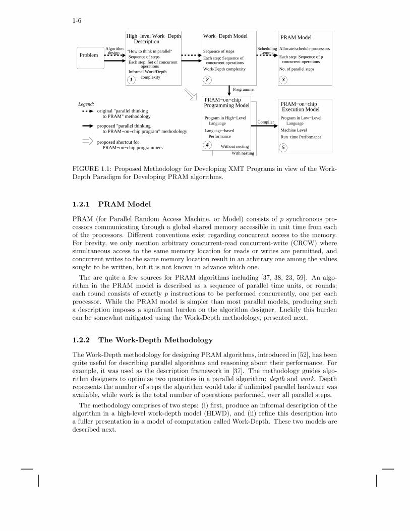
Figure 1.1 depicts the proposed methodology. For context, the figure also depicts thewidely used Work-Depth methodology for advancing from concept to a PRAM algorithm,namely, the sequence of models 1 → 2 → 3 in the figure. For developing a XMT imple-mentation, we propose following the sequence of models 1 → 2 → 4 → 5, as follows. Givena specific problem, an algorithm design stage will produce a High-Level description of theparallel algorithm, in the form of a sequence of steps, each comprising a set of concurrentoperations (box 1). In a first draft, the set of concurrent operations can be implicitly de-fined. See the BFS example in Section 1.2.2. This first draft is refined to a sequence of stepseach comprising now an ordered sequence of concurrent operations (box 2). Next, the pro-gramming effort amounts to translating this description into a single-program multiple-data(SPMD) program using a high-level XMT programming language (box 4). From this SPMDprogram, a compiler will transform and reorganize the code to achieve the best performancein the target XMT execution model (box 5). As an XMT programmer gains experience,he/she will be able to skip box 2 (the Work-Depth model) and directly advance from box 1(high-Level Work-Depth description) to box 4 (high-level XMT program). We also demon-strate some instances where it may be advantageous to skip box 2 because of some featuresof the programming model (such as some ability to handle nesting of parallelism). In Figure1.1 this shortcut is depicted by the arrow 1 → 4. Much of the current paper is devotedto presenting the methodology and demonstrating it. We start with elaborating on eachmodel.
1-6
1
Description
to PRAM" methodology
proposed "parallel thinkingto PRAM−on−chip program" methodology
original "parallel thinkingLegend:
PRAM−on−chip programmersproposed shortcut for
"How to think in parallel"Sequence of stepsEach step: Set of concurrent
Work−Depth Model
2 3
Allocate/schedule processors
No. of parallel steps
PRAM Model
5
PRAM−on−chip
Without nesting4
Informal Work/Depth
Sequence of stepsEach step: Sequence of p
Program in High−Level Program in Low−Level
Programmer
Problem
Execution ModelPRAM−on−chip
With nesting
SchedulingLemma
Compiler
designAlgorithm
complexity
operationsWork/Depth complexity
Each step: Sequence ofconcurrent operations
Language−based
Language
concurrent operations
Run−time Performance
Machine Level
Language
Performance
High−level Work−Depth
Programming Model
FIGURE 1.1: Proposed Methodology for Developing XMT Programs in view of the Work-Depth Paradigm for Developing PRAM algorithms.
1.2.1 PRAM Model
PRAM (for Parallel Random Access Machine, or Model) consists of p synchronous pro-cessors communicating through a global shared memory accessible in unit time from eachof the processors. Different conventions exist regarding concurrent access to the memory.For brevity, we only mention arbitrary concurrent-read concurrent-write (CRCW) wheresimultaneous access to the same memory location for reads or writes are permitted, andconcurrent writes to the same memory location result in an arbitrary one among the valuessought to be written, but it is not known in advance which one.
The are quite a few sources for PRAM algorithms including [37, 38, 23, 59]. An algo-rithm in the PRAM model is described as a sequence of parallel time units, or rounds;each round consists of exactly p instructions to be performed concurrently, one per eachprocessor. While the PRAM model is simpler than most parallel models, producing sucha description imposes a significant burden on the algorithm designer. Luckily this burdencan be somewhat mitigated using the Work-Depth methodology, presented next.
1.2.2 The Work-Depth Methodology
The Work-Depth methodology for designing PRAM algorithms, introduced in [52], has beenquite useful for describing parallel algorithms and reasoning about their performance. Forexample, it was used as the description framework in [37]. The methodology guides algo-rithm designers to optimize two quantities in a parallel algorithm: depth and work. Depthrepresents the number of steps the algorithm would take if unlimited parallel hardware wasavailable, while work is the total number of operations performed, over all parallel steps.
The methodology comprises of two steps: (i) first, produce an informal description of thealgorithm in a high-level work-depth model (HLWD), and (ii) refine this description intoa fuller presentation in a model of computation called Work-Depth. These two models aredescribed next.
Advancing PRAM Algorithms into Parallel Programs 1-7
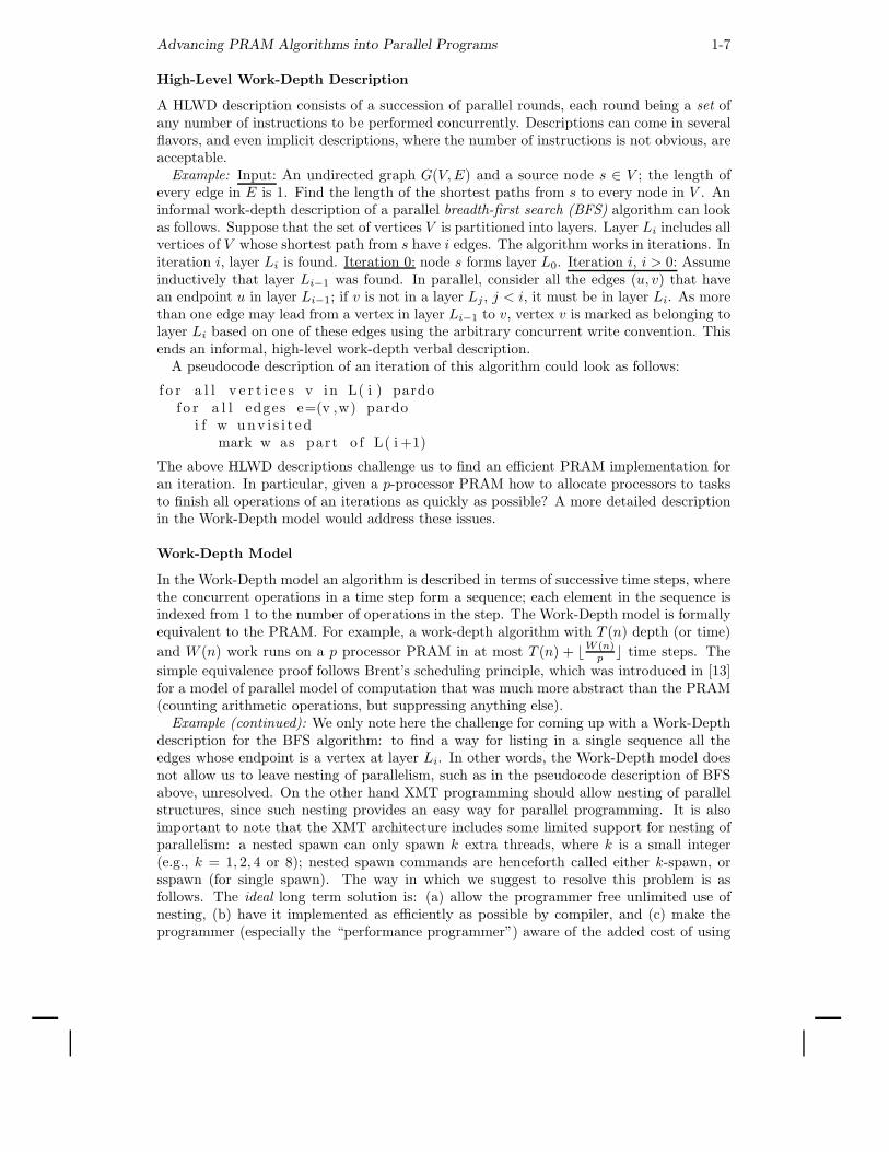
High-Level Work-Depth Description
A HLWD description consists of a succession of parallel rounds, each round being a set ofany number of instructions to be performed concurrently. Descriptions can come in severalflavors, and even implicit descriptions, where the number of instructions is not obvious, areacceptable.
Example: Input: An undirected graph G(V, E) and a source node s ∈ V ; the length ofevery edge in E is 1. Find the length of the shortest paths from s to every node in V . Aninformal work-depth description of a parallel breadth-first search (BFS) algorithm can lookas follows. Suppose that the set of vertices V is partitioned into layers. Layer Li includes allvertices of V whose shortest path from s have i edges. The algorithm works in iterations. Initeration i, layer Li is found. Iteration 0: node s forms layer L0. Iteration i, i > 0: Assumeinductively that layer Li−1 was found. In parallel, consider all the edges (u, v) that havean endpoint u in layer Li−1; if v is not in a layer Lj , j < i, it must be in layer Li. As morethan one edge may lead from a vertex in layer Li−1 to v, vertex v is marked as belonging tolayer Li based on one of these edges using the arbitrary concurrent write convention. Thisends an informal, high-level work-depth verbal description.
A pseudocode description of an iteration of this algorithm could look as follows:
f o r a l l v e r t i c e s v in L( i ) pardof o r a l l edges e=(v ,w) pardo
i f w unv i s i t e dmark w as part o f L( i +1)
The above HLWD descriptions challenge us to find an efficient PRAM implementation foran iteration. In particular, given a p-processor PRAM how to allocate processors to tasksto finish all operations of an iterations as quickly as possible? A more detailed descriptionin the Work-Depth model would address these issues.
Work-Depth Model
In the Work-Depth model an algorithm is described in terms of successive time steps, wherethe concurrent operations in a time step form a sequence; each element in the sequence isindexed from 1 to the number of operations in the step. The Work-Depth model is formallyequivalent to the PRAM. For example, a work-depth algorithm with T (n) depth (or time)
and W (n) work runs on a p processor PRAM in at most T (n) + ⌊W (n)p ⌋ time steps. The
simple equivalence proof follows Brent’s scheduling principle, which was introduced in [13]for a model of parallel model of computation that was much more abstract than the PRAM(counting arithmetic operations, but suppressing anything else).
Example (continued): We only note here the challenge for coming up with a Work-Depthdescription for the BFS algorithm: to find a way for listing in a single sequence all theedges whose endpoint is a vertex at layer Li. In other words, the Work-Depth model doesnot allow us to leave nesting of parallelism, such as in the pseudocode description of BFSabove, unresolved. On the other hand XMT programming should allow nesting of parallelstructures, since such nesting provides an easy way for parallel programming. It is alsoimportant to note that the XMT architecture includes some limited support for nesting ofparallelism: a nested spawn can only spawn k extra threads, where k is a small integer(e.g., k = 1, 2, 4 or 8); nested spawn commands are henceforth called either k-spawn, orsspawn (for single spawn). The way in which we suggest to resolve this problem is asfollows. The ideal long term solution is: (a) allow the programmer free unlimited use ofnesting, (b) have it implemented as efficiently as possible by compiler, and (c) make theprogrammer (especially the “performance programmer”) aware of the added cost of using
1-8
nesting. However, since our compiler is not yet mature enough to handle this matter, ourtentative short term solution is presented in Section 1.8, which shows how to build on thesupport for nesting provided by the architecture. There is merit to this “manual solution”beyond its tentative role until the compiler matures. Such solution should still need to beunderstood (even after the ideal compiler solution is in place) by performance programmers,so that the impact of nesting on performance is clear to them.
The reason for bringing this issue up this early in the discussion is that it actually demon-strates that our methodology can sometimes proceed directly to the PRAM-like program-ming methodology, rather than make a “stop” at the Work-Depth model.
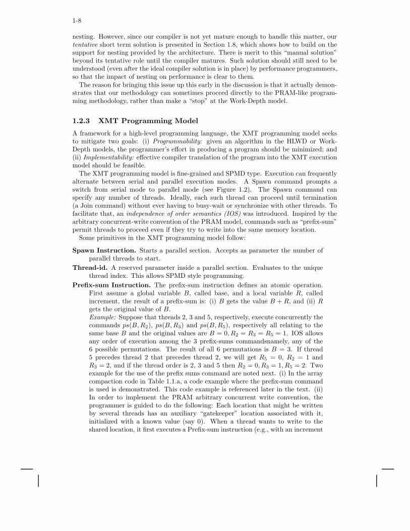
1.2.3 XMT Programming Model
A framework for a high-level programming language, the XMT programming model seeksto mitigate two goals: (i) Programmability: given an algorithm in the HLWD or Work-Depth models, the programmer’s effort in producing a program should be minimized; and(ii) Implementability: effective compiler translation of the program into the XMT executionmodel should be feasible.
The XMT programming model is fine-grained and SPMD type. Execution can frequentlyalternate between serial and parallel execution modes. A Spawn command prompts aswitch from serial mode to parallel mode (see Figure 1.2). The Spawn command canspecify any number of threads. Ideally, each such thread can proceed until termination(a Join command) without ever having to busy-wait or synchronize with other threads. Tofacilitate that, an independence of order semantics (IOS) was introduced. Inspired by thearbitrary concurrent-write convention of the PRAM model, commands such as “prefix-sum”permit threads to proceed even if they try to write into the same memory location.
Some primitives in the XMT programming model follow:
Spawn Instruction. Starts a parallel section. Accepts as parameter the number ofparallel threads to start.
Thread-id. A reserved parameter inside a parallel section. Evaluates to the uniquethread index. This allows SPMD style programming.
Prefix-sum Instruction. The prefix-sum instruction defines an atomic operation.First assume a global variable B, called base, and a local variable R, calledincrement, the result of a prefix-sum is: (i) B gets the value B + R, and (ii) Rgets the original value of B.Example: Suppose that threads 2, 3 and 5, respectively, execute concurrently thecommands ps(B, R2), ps(B, R3) and ps(B, R5), respectively all relating to thesame base B and the original values are B = 0, R2 = R3 = R5 = 1. IOS allowsany order of execution among the 3 prefix-sums commandsnamely, any of the6 possible permutations. The result of all 6 permutations is B = 3. If thread5 precedes thread 2 that precedes thread 2, we will get R5 = 0, R2 = 1 andR3 = 2, and if the thread order is 2, 3 and 5 then R2 = 0, R3 = 1, R5 = 2. Twoexample for the use of the prefix sums command are noted next. (i) In the arraycompaction code in Table 1.1.a, a code example where the prefix-sum commandis used is demonstrated. This code example is referenced later in the text. (ii)In order to implement the PRAM arbitrary concurrent write convention, theprogrammer is guided to do the following: Each location that might be writtenby several threads has an auxiliary “gatekeeper” location associated with it,initialized with a known value (say 0). When a thread wants to write to theshared location, it first executes a Prefix-sum instruction (e.g., with an increment
Advancing PRAM Algorithms into Parallel Programs 1-9
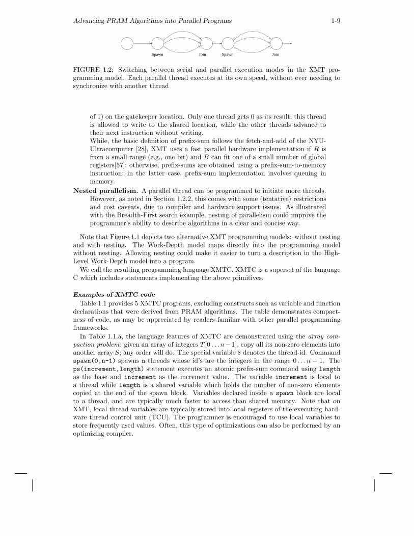
Spawn Join Spawn Join
FIGURE 1.2: Switching between serial and parallel execution modes in the XMT pro-gramming model. Each parallel thread executes at its own speed, without ever needing tosynchronize with another thread
of 1) on the gatekeeper location. Only one thread gets 0 as its result; this threadis allowed to write to the shared location, while the other threads advance totheir next instruction without writing.While, the basic definition of prefix-sum follows the fetch-and-add of the NYU-Ultracomputer [28], XMT uses a fast parallel hardware implementation if R isfrom a small range (e.g., one bit) and B can fit one of a small number of globalregisters[57]; otherwise, prefix-sums are obtained using a prefix-sum-to-memoryinstruction; in the latter case, prefix-sum implementation involves queuing inmemory.
Nested parallelism. A parallel thread can be programmed to initiate more threads.However, as noted in Section 1.2.2, this comes with some (tentative) restrictionsand cost caveats, due to compiler and hardware support issues. As illustratedwith the Breadth-First search example, nesting of parallelism could improve theprogrammer’s ability to describe algorithms in a clear and concise way.
Note that Figure 1.1 depicts two alternative XMT programming models: without nestingand with nesting. The Work-Depth model maps directly into the programming modelwithout nesting. Allowing nesting could make it easier to turn a description in the High-Level Work-Depth model into a program.
We call the resulting programming language XMTC. XMTC is a superset of the languageC which includes statements implementing the above primitives.
Examples of XMTC code
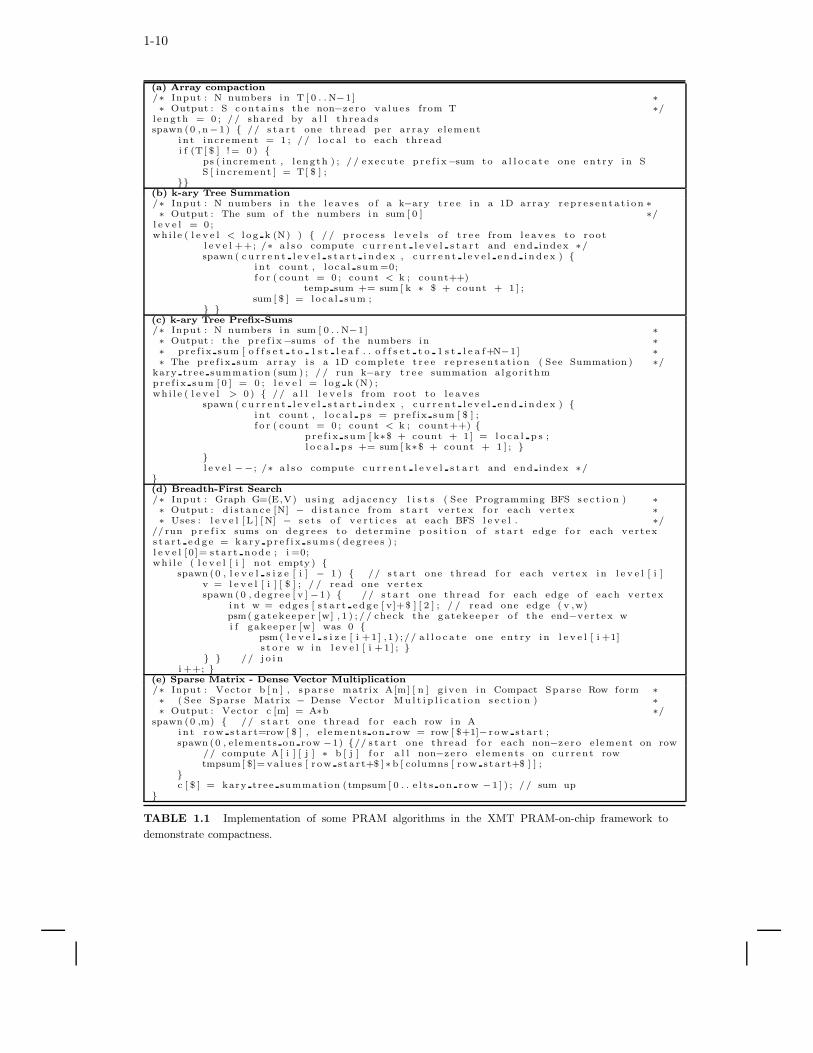
Table 1.1 provides 5 XMTC programs, excluding constructs such as variable and functiondeclarations that were derived from PRAM algorithms. The table demonstrates compact-ness of code, as may be appreciated by readers familiar with other parallel programmingframeworks.
In Table 1.1.a, the language features of XMTC are demonstrated using the array com-paction problem: given an array of integers T [0 . . . n−1], copy all its non-zero elements intoanother array S; any order will do. The special variable $ denotes the thread-id. Commandspawn(0,n-1) spawns n threads whose id’s are the integers in the range 0 . . . n − 1. Theps(increment,length) statement executes an atomic prefix-sum command using length
as the base and increment as the increment value. The variable increment is local toa thread while length is a shared variable which holds the number of non-zero elementscopied at the end of the spawn block. Variables declared inside a spawn block are localto a thread, and are typically much faster to access than shared memory. Note that onXMT, local thread variables are typically stored into local registers of the executing hard-ware thread control unit (TCU). The programmer is encouraged to use local variables tostore frequently used values. Often, this type of optimizations can also be performed by anoptimizing compiler.
1-10
(a) Array compaction/∗ Input : N numbers in T [ 0 . . N−1] ∗∗ Output : S con ta in s the non−ze ro va lues from T ∗/
length = 0 ; / / shared by a l l threadsspawn (0 ,n−1) { // s t a r t one thread per array e lement
in t increment = 1 ; / / l o c a l to each threadi f (T[ $ ] != 0 ) {
ps ( increment , l ength ) ; / / execute p r e f i x−sum to a l l o c a t e one entry in SS [ increment ] = T[ $ ] ;
}}(b) k-ary Tree Summation/∗ Input : N numbers in the l e ave s o f a k−ary t r e e in a 1D array r ep r e s en ta t i on ∗∗ Output : The sum o f the numbers in sum [ 0 ] ∗/
l e v e l = 0;whi l e ( l e v e l < l o g k (N) ) { / / p roc e s s l e v e l s o f t r e e from l e ave s to root
l e v e l ++; /∗ a l s o compute c u r r e n t l e v e l s t a r t and end index ∗/spawn ( c u r r e n t l e v e l s t a r t i n d e x , cu r r e n t l e v e l en d in d ex ) {
i n t count , loca l sum =0;f o r ( count = 0 ; count < k ; count++)
temp sum += sum [ k ∗ $ + count + 1 ] ;sum [ $ ] = loca l sum ;
} }(c) k-ary Tree Prefix-Sums/∗ Input : N numbers in sum [ 0 . . N−1] ∗∗ Output : the p r e f i x−sums o f the numbers in ∗∗ pre f ix sum [ o f f s e t t o 1 s t l e a f . . o f f s e t t o 1 s t l e a f+N−1] ∗∗ The pre f ix sum array i s a 1D complete t r e e r ep r e s en ta t i on ( See Summation ) ∗/
kary tree summation (sum ) ; / / run k−ary t r e e summation a lgor i thmpre f ix sum [ 0 ] = 0 ; l e v e l = l og k (N) ;wh i l e ( l e v e l > 0 ) { // a l l l e v e l s from root to l e ave s
spawn ( c u r r e n t l e v e l s t a r t i n d e x , cu r r e n t l e v e l en d in d ex ) {i n t count , l o c a l p s = pre f ix sum [ $ ] ;f o r ( count = 0 ; count < k ; count++) {
pre f ix sum [ k∗$ + count + 1] = l o c a l p s ;l o c a l p s += sum [ k∗$ + count + 1 ] ; }
}l e v e l −−; /∗ a l s o compute c u r r e n t l e v e l s t a r t and end index ∗/
}(d) Breadth-First Search/∗ Input : Graph G=(E,V) us ing adjacency l i s t s ( See Programming BFS s e c t i o n ) ∗∗ Output : d i s t anc e [N] − d i s t anc e from s t a r t ve rtex f o r each vertex ∗∗ Uses : l e v e l [ L ] [N] − s e t s o f v e r t i c e s at each BFS l e v e l . ∗/
// run p r e f i x sums on degree s to determine p o s i t i o n o f s t a r t edge f o r each vertexs t a r t ed g e = kary p r e f i x sums ( degree s ) ;l e v e l [0]= s ta r t node ; i =0;whi l e ( l e v e l [ i ] not empty ) {
spawn (0 , l e v e l s i z e [ i ] − 1 ) { // s t a r t one thread f o r each vertex in l e v e l [ i ]v = l e v e l [ i ] [ $ ] ; / / read one vertexspawn (0 , degree [ v ] −1) { // s t a r t one thread f o r each edge o f each vertex
in t w = edges [ s t a r t edg e [ v]+$ ] [ 2 ] ; / / read one edge ( v ,w)psm( gatekeeper [w] , 1 ) ; / / check the gatekeeper o f the end−vertex wi f gakeeper [w ] was 0 {
psm( l e v e l s i z e [ i +1] ,1) ;// a l l o c a t e one entry in l e v e l [ i +1]s t o r e w in l e v e l [ i +1 ] ; }
} } // j o i ni ++; }
(e) Sparse Matrix - Dense Vector Multiplication/∗ Input : Vector b [ n ] , spa r s e matrix A[m] [ n ] g iven in Compact Sparse Row form ∗∗ ( See Sparse Matrix − Dense Vector Mu l t i p l i c a t i on s e c t i o n ) ∗∗ Output : Vector c [m] = A∗b ∗/
spawn (0 ,m) { // s t a r t one thread f o r each row in Ain t row sta r t=row [ $ ] , e l ements on row = row [ $+1]− r ow sta r t ;spawn (0 , e lements on row −1) {// s t a r t one thread f o r each non−ze ro e lement on row
// compute A[ i ] [ j ] ∗ b [ j ] f o r a l l non−ze ro e lements on current rowtmpsum[ $]= values [ r ow sta r t+$ ]∗b [ columns [ r ow sta r t+$ ] ] ;
}c [ $ ] = kary tree summation (tmpsum [ 0 . . e l t s on row −1 ] ) ; / / sum up
}
TABLE 1.1 Implementation of some PRAM algorithms in the XMT PRAM-on-chip framework to
demonstrate compactness.
Advancing PRAM Algorithms into Parallel Programs 1-11
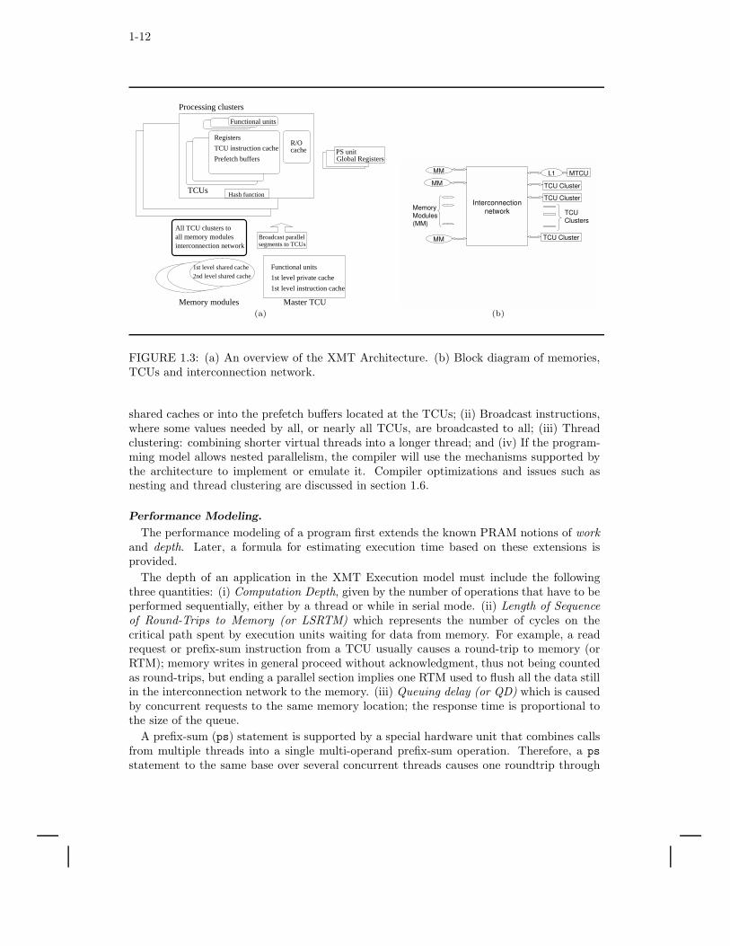
To evaluate performance in this model, a Language-Based Performance Model is used:performance costs are assigned to each primitive instruction in the language with someaccounting rules added for the performance cost of computer programs (e.g., depending onexecution sequences). Such performance modeling was used by Aho and Ullman [1] and wasgeneralized for parallelism by Blelloch [10]. The paper [20] used language-based modelingfor studying parallel list ranking relative to an earlier performance model for XMT.
1.2.4 XMT Execution Model
The execution model depends on XMT architecture choices. However, as can be seen fromthe modeling itself, this dependence is rather minimal and should not compromise the gener-ality of the model for other future chip-multiprocessing architectures whose general featuresare similar. We only review the architecture below and refer to [47] for a fuller description.Class presentation of the overall methodology proposed in the current paper usually breakshere to review, based on [47], the way in which: (i) the XMT apparatus of the programcounters and stored program extends the (well-known) von-Neumann serial apparatus, (ii)the switch from serial to parallel mode and back to serial mode is implemented, (iii) vir-tual threads coming from an XMTC program are allocated dynamically at run time, forload balancing, to thread control units (TCUs), (iv) hardware implementation of prefix-sumenhances the computation, and (v) independence of order semantics (IOS), in particular,and the overall design principle of no-busy-wait finite-state-machines (NBW FSM), in gen-eral, allow making as much progress as possible with whatever data and instructions areavailable.
Possible architecture choices.
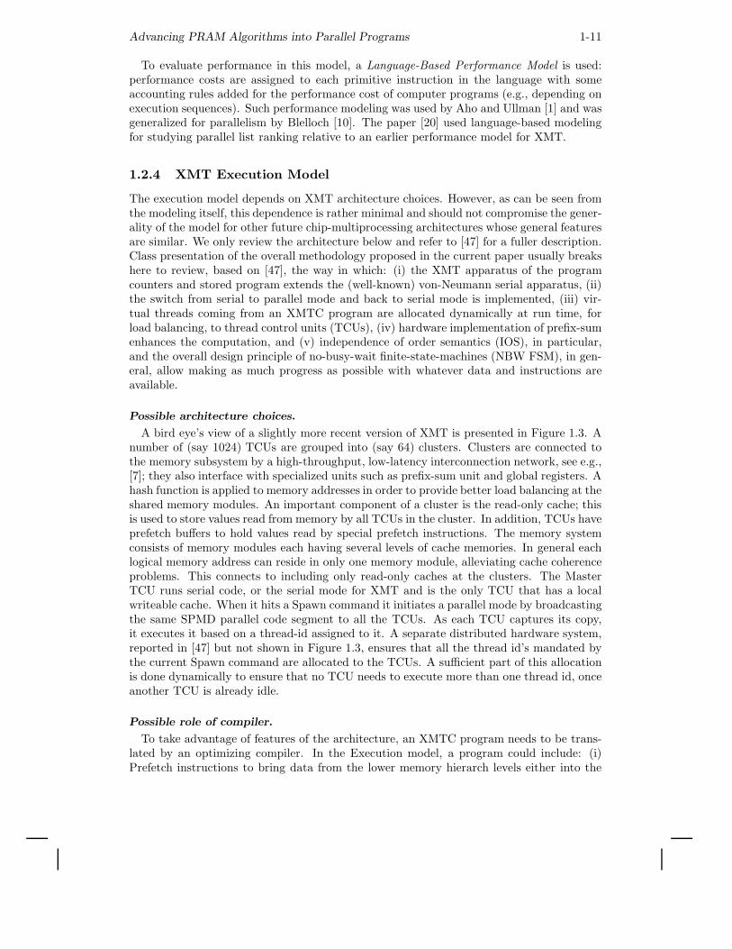
A bird eye’s view of a slightly more recent version of XMT is presented in Figure 1.3. Anumber of (say 1024) TCUs are grouped into (say 64) clusters. Clusters are connected tothe memory subsystem by a high-throughput, low-latency interconnection network, see e.g.,[7]; they also interface with specialized units such as prefix-sum unit and global registers. Ahash function is applied to memory addresses in order to provide better load balancing at theshared memory modules. An important component of a cluster is the read-only cache; thisis used to store values read from memory by all TCUs in the cluster. In addition, TCUs haveprefetch buffers to hold values read by special prefetch instructions. The memory systemconsists of memory modules each having several levels of cache memories. In general eachlogical memory address can reside in only one memory module, alleviating cache coherenceproblems. This connects to including only read-only caches at the clusters. The MasterTCU runs serial code, or the serial mode for XMT and is the only TCU that has a localwriteable cache. When it hits a Spawn command it initiates a parallel mode by broadcastingthe same SPMD parallel code segment to all the TCUs. As each TCU captures its copy,it executes it based on a thread-id assigned to it. A separate distributed hardware system,reported in [47] but not shown in Figure 1.3, ensures that all the thread id’s mandated bythe current Spawn command are allocated to the TCUs. A sufficient part of this allocationis done dynamically to ensure that no TCU needs to execute more than one thread id, onceanother TCU is already idle.
Possible role of compiler.
To take advantage of features of the architecture, an XMTC program needs to be trans-lated by an optimizing compiler. In the Execution model, a program could include: (i)Prefetch instructions to bring data from the lower memory hierarch levels either into the
1-12
Master TCUMemory modules
Registers
TCU instruction cache
TCUs
Functional units
1st level private cache
1st level instruction cache
Functional units
PS unit
Broadcast parallel segments to TCUs
2nd level shared cache1st level shared cache
Processing clusters
R/Ocache
Prefetch buffers
Hash function
All TCU clusters toall memory modulesinterconnection network
Global Registers
(a) (b)
FIGURE 1.3: (a) An overview of the XMT Architecture. (b) Block diagram of memories,TCUs and interconnection network.
shared caches or into the prefetch buffers located at the TCUs; (ii) Broadcast instructions,where some values needed by all, or nearly all TCUs, are broadcasted to all; (iii) Threadclustering: combining shorter virtual threads into a longer thread; and (iv) If the program-ming model allows nested parallelism, the compiler will use the mechanisms supported bythe architecture to implement or emulate it. Compiler optimizations and issues such asnesting and thread clustering are discussed in section 1.6.
Performance Modeling.
The performance modeling of a program first extends the known PRAM notions of workand depth. Later, a formula for estimating execution time based on these extensions isprovided.
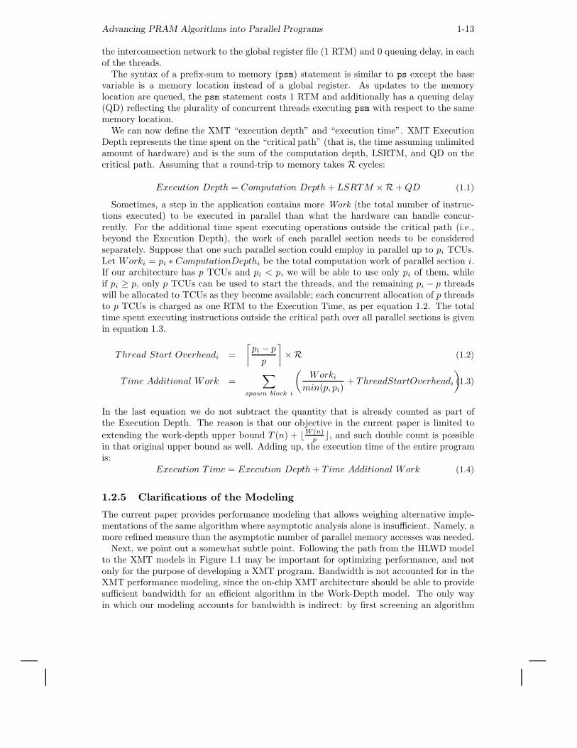
The depth of an application in the XMT Execution model must include the followingthree quantities: (i) Computation Depth, given by the number of operations that have to beperformed sequentially, either by a thread or while in serial mode. (ii) Length of Sequenceof Round-Trips to Memory (or LSRTM) which represents the number of cycles on thecritical path spent by execution units waiting for data from memory. For example, a readrequest or prefix-sum instruction from a TCU usually causes a round-trip to memory (orRTM); memory writes in general proceed without acknowledgment, thus not being countedas round-trips, but ending a parallel section implies one RTM used to flush all the data stillin the interconnection network to the memory. (iii) Queuing delay (or QD) which is causedby concurrent requests to the same memory location; the response time is proportional tothe size of the queue.
A prefix-sum (ps) statement is supported by a special hardware unit that combines callsfrom multiple threads into a single multi-operand prefix-sum operation. Therefore, a ps
statement to the same base over several concurrent threads causes one roundtrip through
Advancing PRAM Algorithms into Parallel Programs 1-13
the interconnection network to the global register file (1 RTM) and 0 queuing delay, in eachof the threads.
The syntax of a prefix-sum to memory (psm) statement is similar to ps except the basevariable is a memory location instead of a global register. As updates to the memorylocation are queued, the psm statement costs 1 RTM and additionally has a queuing delay(QD) reflecting the plurality of concurrent threads executing psm with respect to the samememory location.
We can now define the XMT “execution depth” and “execution time”. XMT ExecutionDepth represents the time spent on the “critical path” (that is, the time assuming unlimitedamount of hardware) and is the sum of the computation depth, LSRTM, and QD on thecritical path. Assuming that a round-trip to memory takes R cycles:
Execution Depth = Computation Depth + LSRTM ×R + QD (1.1)
Sometimes, a step in the application contains more Work (the total number of instruc-tions executed) to be executed in parallel than what the hardware can handle concur-rently. For the additional time spent executing operations outside the critical path (i.e.,beyond the Execution Depth), the work of each parallel section needs to be consideredseparately. Suppose that one such parallel section could employ in parallel up to pi TCUs.Let Worki = pi ∗ ComputationDepthi be the total computation work of parallel section i.If our architecture has p TCUs and pi < p, we will be able to use only pi of them, whileif pi ≥ p, only p TCUs can be used to start the threads, and the remaining pi − p threadswill be allocated to TCUs as they become available; each concurrent allocation of p threadsto p TCUs is charged as one RTM to the Execution Time, as per equation 1.2. The totaltime spent executing instructions outside the critical path over all parallel sections is givenin equation 1.3.
Thread Start Overheadi =
⌈
pi − p
p
⌉
×R (1.2)
T ime Additional Work =∑
spawn block i
(
Worki
min(p, pi)+ ThreadStartOverheadi
)
(1.3)
In the last equation we do not subtract the quantity that is already counted as part ofthe Execution Depth. The reason is that our objective in the current paper is limited to
extending the work-depth upper bound T (n) + ⌊W (n)p ⌋, and such double count is possible
in that original upper bound as well. Adding up, the execution time of the entire programis:
Execution T ime = Execution Depth + T ime Additional Work (1.4)
1.2.5 Clarifications of the Modeling
The current paper provides performance modeling that allows weighing alternative imple-mentations of the same algorithm where asymptotic analysis alone is insufficient. Namely, amore refined measure than the asymptotic number of parallel memory accesses was needed.
Next, we point out a somewhat subtle point. Following the path from the HLWD modelto the XMT models in Figure 1.1 may be important for optimizing performance, and notonly for the purpose of developing a XMT program. Bandwidth is not accounted for in theXMT performance modeling, since the on-chip XMT architecture should be able to providesufficient bandwidth for an efficient algorithm in the Work-Depth model. The only wayin which our modeling accounts for bandwidth is indirect: by first screening an algorithm
1-14
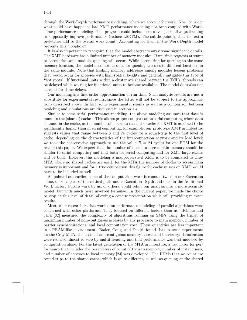
through the Work-Depth performance modeling, where we account for work. Now, considerwhat could have happened had XMT performance modeling not been coupled with Work-Time performance modeling. The program could include excessive speculative prefetchingto supposedly improve performance (reduce LSRTM). The subtle point is that the extraprefetches add to the overall work count. Accounting for them in the Work-Depth modelprevents this “loophole”.
It is also important to recognize that the model abstracts away some significant details.The XMT hardware has a limited number of memory modules. If multiple requests attemptto access the same module, queuing will occur. While accounting for queuing to the samememory location, the model does not account for queuing accesses to different locations inthe same module. Note that hashing memory addresses among modules lessens problemsthat would occur for accesses with high spatial locality and generally mitigates this type of“hot spots”. If functional units within a cluster are shared between the TCUs, threads canbe delayed while waiting for functional units to become available. The model does also notaccount for these delays.
Our modeling is a first-order approximation of run time. Such analytic results are not asubstitute for experimental results, since the latter will not be subject to the approxima-tions described above. In fact, some experimental results as well as a comparison betweenmodeling and simulations are discussed in section 1.4.
Similar to some serial performance modeling, the above modeling assumes that data isfound in the (shared) caches. This allows proper comparison to serial computing where datais found in the cache, as the number of clocks to reach the cache for XMT is assumed to besignificantly higher than in serial computing; for example, our prototype XMT architecturesuggests values that range between 6 and 24 cycles for a round-trip to the first level ofcache, depending on the characteristics of the interconnection network and its load level;we took the conservative approach to use the value R = 24 cycles for one RTM for therest of this paper. We expect that the number of clocks to access main memory should besimilar to serial computing and that both for serial computing and for XMT large cacheswill be built. However, this modeling is inappropriate if XMT is to be compared to CrayMTA where no shared caches are used: for the MTA the number of clocks to access mainmemory is important and for a true comparison this figure for cache misses on XMT wouldhave to be included as well.
As pointed out earlier, some of the computation work is counted twice in our ExecutionTime, once as part of the critical path under Execution Depth and once in the AdditionalWork factor. Future work by us, or others, could refine our analysis into a more accuratemodel, but with much more involved formulae. In the current paper, we made the choiceto stop at this level of detail allowing a concise presentation while still providing relevantresults.
Most other researchers that worked on performance modeling of parallel algorithms wereconcerned with other platforms. They focused on different factors than us. Helman andJaJa [32] measured the complexity of algorithms running on SMPs using the triplet ofmaximum number of non-contiguous accesses by any processor to main memory, number ofbarrier synchronizations, and local computation cost. These quantities are less importantin a PRAM-like environment. Bader, Cong, and Feo [6] found that in some experimentson the Cray MTA, the costs of non-contiguous memory access and barrier synchronizationwere reduced almost to zero by multithreading and that performance was best modeled bycomputation alone. For the latest generation of the MTA architecture, a calculator for per-formance that includes the parameters of count of trips to memory, number of instructions,and number of accesses to local memory [24] was developed. The RTMs that we count areround trips to the shared cache, which is quite different, as well as queuing at the shared
Advancing PRAM Algorithms into Parallel Programs 1-15
cache. Another significant difference is that we consider the effect of optimizations such asprefetch and thread clustering. Nevertheless, the calculator should provide an interestingbasis for comparison between performance of applications on MTA and XMT. The incor-poration of queuing follows the well-known QRQW PRAM model of Gibbons, Matias andRamachandran [27]. A succinct way to summarize the modeling contribution of the cur-rent paper is that unlike previous practice QRQW becomes secondary, though still quiteimportant, to LSRTM.
1.3 An Example for Using the Methodology: Summation
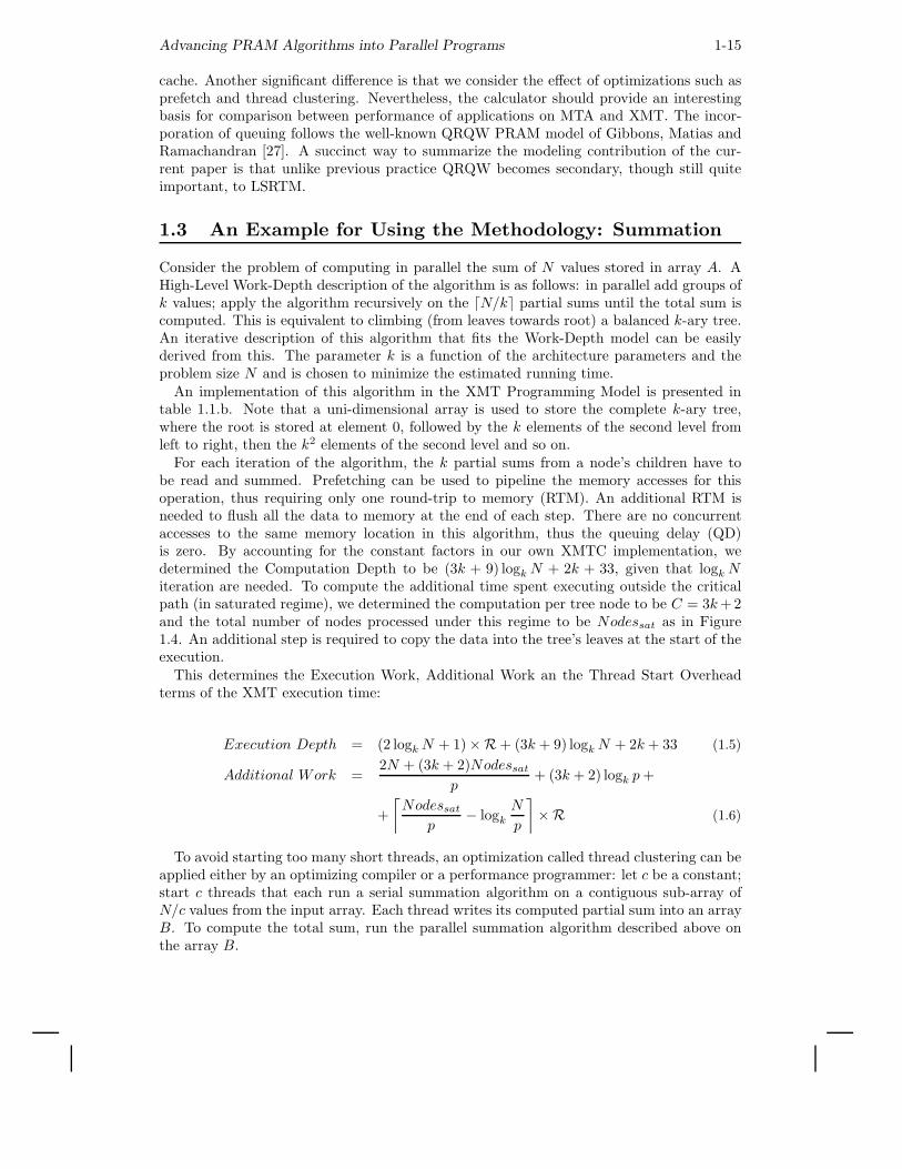
Consider the problem of computing in parallel the sum of N values stored in array A. AHigh-Level Work-Depth description of the algorithm is as follows: in parallel add groups ofk values; apply the algorithm recursively on the ⌈N/k⌉ partial sums until the total sum iscomputed. This is equivalent to climbing (from leaves towards root) a balanced k-ary tree.An iterative description of this algorithm that fits the Work-Depth model can be easilyderived from this. The parameter k is a function of the architecture parameters and theproblem size N and is chosen to minimize the estimated running time.
An implementation of this algorithm in the XMT Programming Model is presented intable 1.1.b. Note that a uni-dimensional array is used to store the complete k-ary tree,where the root is stored at element 0, followed by the k elements of the second level fromleft to right, then the k2 elements of the second level and so on.
For each iteration of the algorithm, the k partial sums from a node’s children have tobe read and summed. Prefetching can be used to pipeline the memory accesses for thisoperation, thus requiring only one round-trip to memory (RTM). An additional RTM isneeded to flush all the data to memory at the end of each step. There are no concurrentaccesses to the same memory location in this algorithm, thus the queuing delay (QD)is zero. By accounting for the constant factors in our own XMTC implementation, wedetermined the Computation Depth to be (3k + 9) logk N + 2k + 33, given that logk Niteration are needed. To compute the additional time spent executing outside the criticalpath (in saturated regime), we determined the computation per tree node to be C = 3k +2and the total number of nodes processed under this regime to be Nodessat as in Figure1.4. An additional step is required to copy the data into the tree’s leaves at the start of theexecution.
This determines the Execution Work, Additional Work an the Thread Start Overheadterms of the XMT execution time:
Execution Depth = (2 logk N + 1) ×R + (3k + 9) logk N + 2k + 33 (1.5)
Additional Work =2N + (3k + 2)Nodessat
p+ (3k + 2) logk p +
+
⌈
Nodessat
p− logk
N
p
⌉
×R (1.6)
To avoid starting too many short threads, an optimization called thread clustering can beapplied either by an optimizing compiler or a performance programmer: let c be a constant;start c threads that each run a serial summation algorithm on a contiguous sub-array ofN/c values from the input array. Each thread writes its computed partial sum into an arrayB. To compute the total sum, run the parallel summation algorithm described above onthe array B.
1-16
logkp Levels
p
Nodessat=
logk p
Leaveswith no work
N
Sub−saturatedregime
Saturatedregime
N−min(p,N−1)−1
k−1
−1 LevelsN
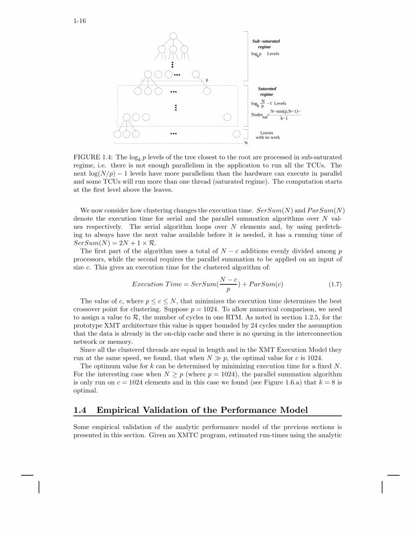
FIGURE 1.4: The logk p levels of the tree closest to the root are processed in sub-saturatedregime, i.e. there is not enough parallelism in the application to run all the TCUs. Thenext log(N/p) − 1 levels have more parallelism than the hardware can execute in paralleland some TCUs will run more than one thread (saturated regime). The computation startsat the first level above the leaves.
We now consider how clustering changes the execution time. SerSum(N) and ParSum(N)denote the execution time for serial and the parallel summation algorithms over N val-ues respectively. The serial algorithm loops over N elements and, by using prefetch-ing to always have the next value available before it is needed, it has a running time ofSerSum(N) = 2N + 1 ×R.
The first part of the algorithm uses a total of N − c additions evenly divided among pprocessors, while the second requires the parallel summation to be applied on an input ofsize c. This gives an execution time for the clustered algorithm of:
Execution T ime = SerSum(N − c
p) + ParSum(c) (1.7)
The value of c, where p ≤ c ≤ N , that minimizes the execution time determines the bestcrossover point for clustering. Suppose p = 1024. To allow numerical comparison, we needto assign a value to R, the number of cycles in one RTM. As noted in section 1.2.5, for theprototype XMT architecture this value is upper bounded by 24 cycles under the assumptionthat the data is already in the on-chip cache and there is no queuing in the interconnectionnetwork or memory.
Since all the clustered threads are equal in length and in the XMT Execution Model theyrun at the same speed, we found, that when N ≫ p, the optimal value for c is 1024.
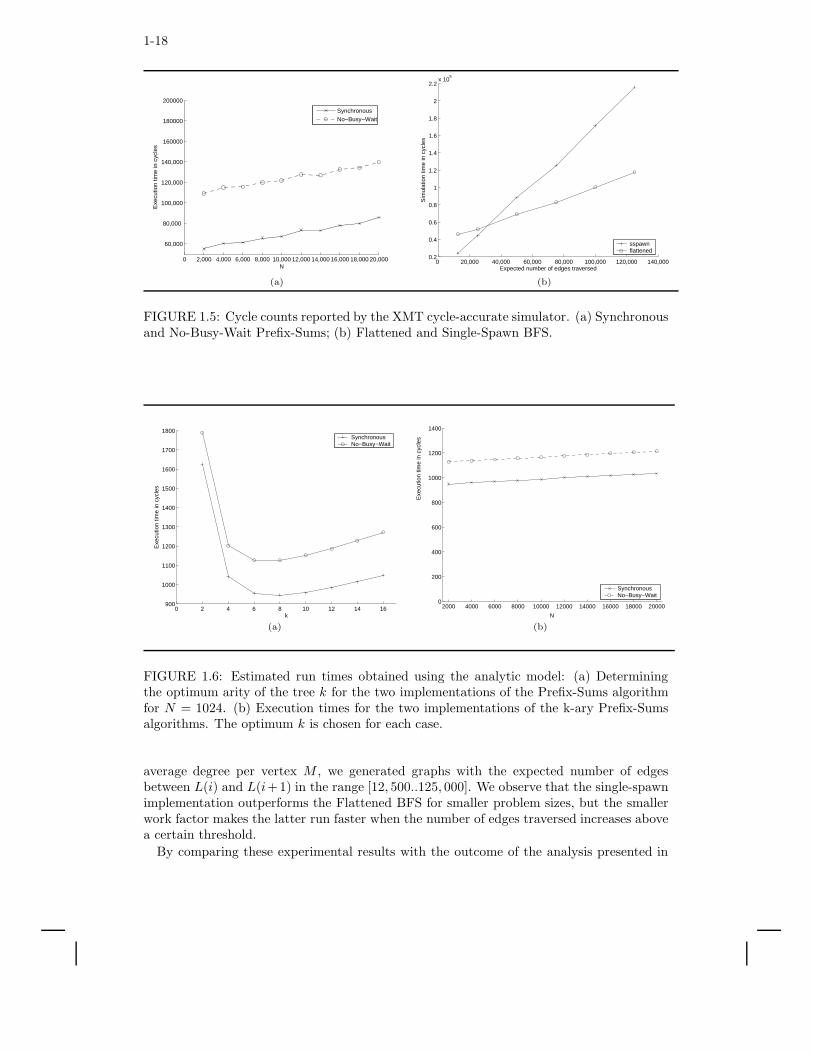
The optimum value for k can be determined by minimizing execution time for a fixed N .For the interesting case when N ≥ p (where p = 1024), the parallel summation algorithmis only run on c = 1024 elements and in this case we found (see Figure 1.6.a) that k = 8 isoptimal.
1.4 Empirical Validation of the Performance Model
Some empirical validation of the analytic performance model of the previous sections ispresented in this section. Given an XMTC program, estimated run-times using the analytic
Advancing PRAM Algorithms into Parallel Programs 1-17
model are compared against simulated run-times using our XMT simulator. Derived froma synthesizable gate-level description of the XMT architecture, the XMT simulation engineaims at being cycle-accurate. A typical configuration includes 1024 thread control units(TCUs) grouped in 64 clusters and one Master TCU.
A gap between the simulations and the analytic model is to be expected. Not only thatthe analytic model as presented makes some simplifying assumptions, such as countingeach XMTC statement as one cycle, and ignoring contention at the functional units, itprovides the same (worst-case) run-time estimates for different input data as long as theinput has the same size. On the other hand, at the present time the XMTC compiler andthe XMT cycle-accurate simulator lack a number of features that were assumed for theanalytic performance model. More specifically, there is no compiler support for prefetchingand thread clustering, and only limited broadcasting capabilities are included. (Also, asleep-wait mechanism noted in Section 1.6.1 is not fully implemented in the simulator,making the single-spawning mechanism less efficient.) All these factors could cause thesimulated run-times to be higher than the ones computed by the analytic approach. Forthat reason, we limit our focus to just studying the relative performance of two or moreimplementations that solve the same problem. This will enable evaluating programmingimplementation approaches against the relative performance gain – one of the goals of thefull paper.
More information about the XMTC compiler and the XMT cycle-accurate simulator canbe found in [8]. An updated version of that document which reflects the most recent versionof the XMT compiler and simulator is available from http://www.umiacs.umd.edu/users/
vishkin/XMT/XMTCManual.pdf andhttp://www.umiacs.umd.edu/users/vishkin/XMT/XMTCTutorial.pdf.
We proceed to describe our experimental results.
1.4.1 Performance Comparison of Implementations
The first experiment consisted of running the implementations of the Prefix-Sums [41, 58]and the parallel Breadth-First Search algorithms discussed in sections 1.7 and 1.8 using theXMT simulator.
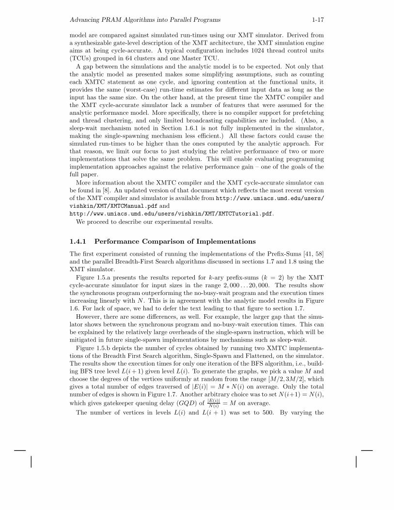
Figure 1.5.a presents the results reported for k-ary prefix-sums (k = 2) by the XMTcycle-accurate simulator for input sizes in the range 2, 000 . . .20, 000. The results showthe synchronous program outperforming the no-busy-wait program and the execution timesincreasing linearly with N . This is in agreement with the analytic model results in Figure1.6. For lack of space, we had to defer the text leading to that figure to section 1.7.
However, there are some differences, as well. For example, the larger gap that the simu-lator shows between the synchronous program and no-busy-wait execution times. This canbe explained by the relatively large overheads of the single-spawn instruction, which will bemitigated in future single-spawn implementations by mechanisms such as sleep-wait.
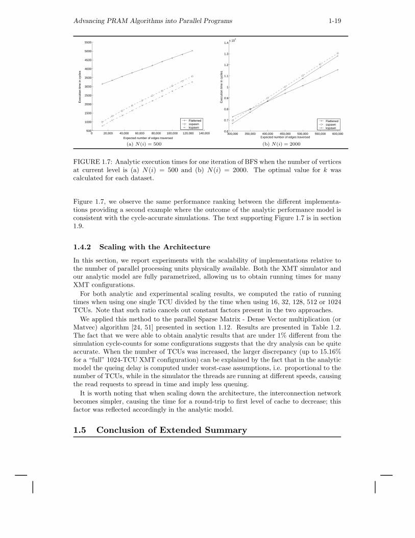
Figure 1.5.b depicts the number of cycles obtained by running two XMTC implementa-tions of the Breadth First Search algorithm, Single-Spawn and Flattened, on the simulator.The results show the execution times for only one iteration of the BFS algorithm, i.e., build-ing BFS tree level L(i + 1) given level L(i). To generate the graphs, we pick a value M andchoose the degrees of the vertices uniformly at random from the range [M/2, 3M/2], whichgives a total number of edges traversed of |E(i)| = M ∗ N(i) on average. Only the totalnumber of edges is shown in Figure 1.7. Another arbitrary choice was to set N(i+1) = N(i),
which gives gatekeeper queuing delay (GQD) of |E(i)|N(i) = M on average.
The number of vertices in levels L(i) and L(i + 1) was set to 500. By varying the
1-18
0 2,000 4,000 6,000 8,000 10,000 12,000 14,000 16,000 18,000 20,000
60,000
80,000
100,000
120,000
140,000
160000
180000
200000
N
Exe
cutio
n tim
e in
cyc
les
SynchronousNo−Busy−Wait
0 20,000 40,000 60,000 80,000 100,000 120,000 140,0000.2
0.4
0.6
0.8
1
1.2
1.4
1.6
1.8
2
2.2x 10
5
Expected number of edges traversed
Sim
ulat
ion
time
in c
ycle
s
sspawnflattened
(a) (b)
FIGURE 1.5: Cycle counts reported by the XMT cycle-accurate simulator. (a) Synchronousand No-Busy-Wait Prefix-Sums; (b) Flattened and Single-Spawn BFS.
0 2 4 6 8 10 12 14 16900
1000
1100
1200
1300
1400
1500
1600
1700
1800
k
Exe
cutio
n tim
e in
cyc
les
SynchronousNo−Busy−Wait
2000 4000 6000 8000 10000 12000 14000 16000 18000 200000
200
400
600
800
1000
1200
1400
N
Exe
cutio
n tim
e in
cyc
les
SynchronousNo−Busy−Wait
(a) (b)
FIGURE 1.6: Estimated run times obtained using the analytic model: (a) Determiningthe optimum arity of the tree k for the two implementations of the Prefix-Sums algorithmfor N = 1024. (b) Execution times for the two implementations of the k-ary Prefix-Sumsalgorithms. The optimum k is chosen for each case.
average degree per vertex M , we generated graphs with the expected number of edgesbetween L(i) and L(i+1) in the range [12, 500..125, 000]. We observe that the single-spawnimplementation outperforms the Flattened BFS for smaller problem sizes, but the smallerwork factor makes the latter run faster when the number of edges traversed increases abovea certain threshold.
By comparing these experimental results with the outcome of the analysis presented in
Advancing PRAM Algorithms into Parallel Programs 1-19
0 20,000 40,000 60,000 80,000 100,000 120,000 140,000500
1000
1500
2000
2500
3000
3500
4000
4500
5000
5500
Expected number of edges traversed
Exe
cutio
n tim
e in
cyc
les
Flattenedsspawnkspawn
300,000 350,000 400,000 450,000 500,000 550,000 600,0000.6
0.7
0.8
0.9
1
1.1
1.2
1.3
1.4x 10
4
Expected number of edges traversed
Exe
cutio
n tim
e in
cyc
les
Flattenedsspawnkspawn
(a) N(i) = 500 (b) N(i) = 2000
FIGURE 1.7: Analytic execution times for one iteration of BFS when the number of verticesat current level is (a) N(i) = 500 and (b) N(i) = 2000. The optimal value for k wascalculated for each dataset.
Figure 1.7, we observe the same performance ranking between the different implementa-tions providing a second example where the outcome of the analytic performance model isconsistent with the cycle-accurate simulations. The text supporting Figure 1.7 is in section1.9.
1.4.2 Scaling with the Architecture
In this section, we report experiments with the scalability of implementations relative tothe number of parallel processing units physically available. Both the XMT simulator andour analytic model are fully parametrized, allowing us to obtain running times for manyXMT configurations.
For both analytic and experimental scaling results, we computed the ratio of runningtimes when using one single TCU divided by the time when using 16, 32, 128, 512 or 1024TCUs. Note that such ratio cancels out constant factors present in the two approaches.
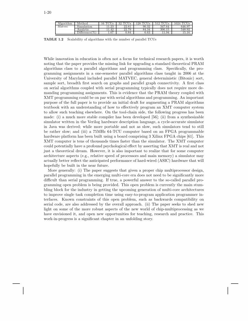
We applied this method to the parallel Sparse Matrix - Dense Vector multiplication (orMatvec) algorithm [24, 51] presented in section 1.12. Results are presented in Table 1.2.The fact that we were able to obtain analytic results that are under 1% different from thesimulation cycle-counts for some configurations suggests that the dry analysis can be quiteaccurate. When the number of TCUs was increased, the larger discrepancy (up to 15.16%for a “full” 1024-TCU XMT configuration) can be explained by the fact that in the analyticmodel the queing delay is computed under worst-case assumptions, i.e. proportional to thenumber of TCUs, while in the simulator the threads are running at different speeds, causingthe read requests to spread in time and imply less queuing.
It is worth noting that when scaling down the architecture, the interconnection networkbecomes simpler, causing the time for a round-trip to first level of cache to decrease; thisfactor was reflected accordingly in the analytic model.
1.5 Conclusion of Extended Summary
1-20
Algorithm Method 16 TCUs 32 TCUs 128 TCUs 512 TCUs 1024 TCUsMatvec Simulation 11.23 22.61 90.32 347.64 646.97
Analytic 11.42 22.79 84.34 306.15 548.92Difference(%) 1.67 0.84 6.63 11.94 15.16
TABLE 1.2 Scalability of algorithms with the number of parallel TCUs
While innovation in education is often not a focus for technical research papers, it is worthnoting that the paper provides the missing link for upgrading a standard theoretical PRAMalgorithms class to a parallel algorithms and programming class. Specifically, the pro-gramming assignments in a one-semester parallel algorithms class taught in 2006 at theUniversity of Maryland included parallel MATVEC, general deterministic (Bitonic) sort,sample sort, breadth first search on graphs and parallel graph connectivity. A first classon serial algorithms coupled with serial programming typically does not require more de-manding programming assignments. This is evidence that the PRAM theory coupled withXMT programming could be on par with serial algorithms and programming. An importantpurpose of the full paper is to provide an initial draft for augmenting a PRAM algorithmstextbook with an understanding of how to effectively program an XMT computer systemto allow such teaching elsewhere. On the tool-chain side, the following progress has beenmade: (i) a much more stable compiler has been developed [56]; (ii) from a synthesizablesimulator written in the Verilog hardware description language, a cycle-accurate simulatorin Java was derived; while more portable and not as slow, such simulators tend to stillbe rather slow; and (iii) a 75MHz 64-TCU computer based on an FPGA programmablehardware platform has been built using a board comprising 3 Xilinx FPGA chips [61]. ThisXMT computer is tens of thousands times faster than the simulator. The XMT computercould potentially have a profound psychological effect by asserting that XMT is real and notjust a theoretical dream. However, it is also important to realize that for some computerarchitecture aspects (e.g., relative speed of processors and main memory) a simulator mayactually better reflect the anticipated performance of hard-wired (ASIC) hardware that willhopefully be built in the near future.
More generally: (i) The paper suggests that given a proper chip multiprocessor design,parallel programming in the emerging multi-core era does not need to be significantly moredifficult than serial programming. If true, a powerful answer to the so-called parallel pro-gramming open problem is being provided. This open problem is currently the main stum-bling block for the industry in getting the upcoming generation of multi-core architecturesto improve single task completion time using easy-to-program application programmer in-terfaces. Known constraints of this open problem, such as backwards compatibility onserial code, are also addressed by the overall approach. (ii) The paper seeks to shed newlight on some of the more robust aspects of the new world of chip-multiprocessing as wehave envisioned it, and open new opportunities for teaching, research and practice. Thiswork-in-progress is a significant chapter in an unfolding story.
Advancing PRAM Algorithms into Parallel Programs 1-21
Part II. Discussion, Examplesand Extensions
1.6 Compiler Optimizations
Given a program in the XMT Programming Model, an optimizing compiler can performvarious transformations on it to better fit the target XMT Execution Model and reduceexecution time. We describe several possible optimizations and demonstrate their effectusing the Summation algorithm described above.
1.6.1 Nested Parallel Sections
Quite a few PRAM algorithms can be expressed with greater clarity and conciseness whennested parallelism is allowed [10]. For this reason, it is desired to allow nesting parallelsections with arbitrary numbers of threads in the XMT Programming Model. Unfortunately,hardware implementation of nesting comes at a cost. The performance programmer needsto be aware of the implementation overheads. To explain a key implementation problemwe need to review the hardware mechanism that allocates threads to the p physical TCUs.Consider an SMPD parallel code section that starts with a spawn(1,n) command, andeach of the n threads ends with a join command without any nested spawns. As notedbefore, the Master TCU broadcasts the parallel code section to all p TCUs. In addition itbroadcasts the number n to all TCUs. TCU i, 1 ≤ i ≤ p, will check whether i > n, and ifnot it will execute thread i; once TCU i hits a join, it will execute a special “system” ps
instruction with an increment of 1 relative to a counter that includes the number of threadsstarted so far; denote the result it gets back by j; if j > n TCU i is done; if not TCU iexecutes thread j; this process is repeated each time a TCU hits a join until all TCUs aredone, when a transition back into serial mode occurs.
Allowing nesting of spawn blocks would require: (i) Upgrading this thread allocationmechanism; the number n representing the total number of threads will be repeatedlyupdated and broadcast to the TCUs. (ii) Facilitating a way for the parent (spawning)thread to pass initialization data to each child (spawned) thread.
In our prototype XMT Programming Model, we allow nested spawns of a small fixednumber of threads through the single-spawn and k-spawn instructions; sspawn starts onesingle additional thread while kspawn starts exactly k threads, where k is a small constant(such as 2 or 4). Each of these instructions causes a delay of one RTM before the parentcan proceed, and an additional delay of 1-2 RTMs before the child thread can proceed (oractually get started). Note that the threads created with a sspawn or kspawn commandwill execute the same code as the original threads, starting with the first instruction in thecurrent parallel section. Suppose that a parent thread wants to create another thread whosevirtual thread number (as referenced from the SPMD code) is v. First, the parent uses asystem ps instruction to a global thread-counter register to create a unique thread ID i forthe child. The parent then enters the value v in A(i), where A is a specially designatedarray in memory. As a result of executing an sspawn or kspawn command by the parentthread: (i) n will be incremented, and at some point in the future (ii) the thread allocationmechanism will generate virtual thread i. The program for thread i starts with reading vthrough A(i). It then can be programmed to use v as its “effective” thread ID.
An algorithm that could benefit from nested spawns is the BFS algorithm. Each iteration
1-22
of the algorithm takes as input Li−1, the set of vertices whose distance from starting vertexs is i − 1 and outputs Li. As noted in section 1.2.2, a simple way to do this is to spawn onethread for each vertex in Li−1, and have each thread spawn as many threads as the numberof its edges.
In the BFS example, the parent thread needs to pass information, such as which edgeto traverse, to child threads. To pass data to the child, the parent writes data in memoryat locations indexed by the child’s ID, using non-blocking writes (namely, the parent sendsout a write request, and can proceed immediately to its next instruction without waitingfor any confirmation). Since it is possible that the child tries to read this data before it isavailable, it should be possible to recognize that the data is not yet there and wait until itis committed to memory. One possible solution for that is described in the next paragraph.The kspawn instruction uses a prefix-sum instruction with increment k to get k thread IDsand proceeds similarly; the delays on the parent and children threads are similar, though afew additional cycles being required for the parent to initialize the data for all k children.
When starting threads using single-spawn or k-spawn, a synchronization step betweenthe parent and the child is necessary to ensure the proper initialization of the latter. Sincewe would rather not use a “busy-wait” synchronization technique that could overload theinterconnection network and waste power, our envisioned XMT architecture would includea special primitive, called sleep-waiting: the memory system holds the read request fromthe child thread until the data is actually committed by the parent thread, and only thensatisfies the request.
When advancing from the programming to the execution model, a compiler can automat-ically transform a nested spawn of n threads, and n can be any number, into a recursiveapplication of single-spawns (or k-spawns). The recursive application divides much of thetask of spawning n thread among the newly spawned threads. When a thread starts a newchild, it assigns to it half (or 1
k+1 for k-spawn) of the n− 1 remaining threads that need tobe spawned. This process proceeds in a recursive manner.
1.6.2 Clustering
The XMT Programming Model allows spawning an arbitrary number of virtual threads,but the architecture has only a limited number of TCUs to run these threads. In theprogression from the Programming Model to the Execution Model, we often need to makea choice between two options: (i) spawn fewer threads each effectively executing severalshorter threads, and (ii) run the shorter threads as is. Combining short threads into alonger thread is called clustering and offers several advantages: (a) reduce RTMs and QDs:we can pipeline memory accesses that had previously been in separate threads; this canreduce extra costs from serialization of RTMs and QDs that are not on the critical path; (b)(reduce thread initiation overhead: spawning fewer threads means reducing thread initiationoverheads, i.e. the time required to start a new thread on a recently freed TCU; (c) reducememory needed: each spawned thread (even those that are waiting for a TCU) usually takesup space in the system memory to store initialization and local data.
Note that if the code provides fewer threads than the hardware can support, there arefew advantages if any to using fewer longer threads. Also, running fewer, longer threadscan adversely affect the automatic load balancing mechanism. Thus, as discussed below,the granularity of the clustering is an issue that needs to be addressed.
In some cases, clustering can be used to group the work of several threads and executethis work using a serial algorithm. For example, in the Summation algorithm the elementsof the input array are placed in the leaves of a k-ary tree, and the algorithm climbs the treecomputing for each node the sum of its children. However, we can instead start with an
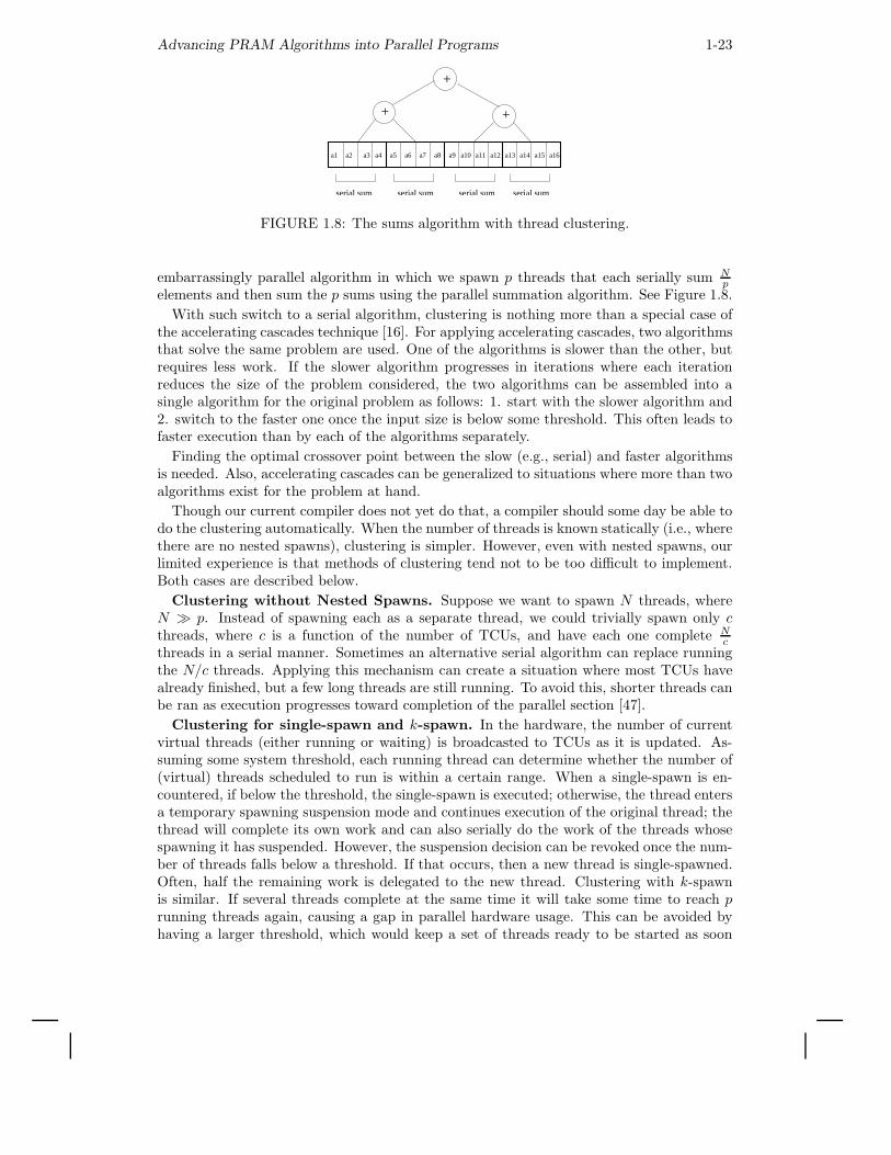
Advancing PRAM Algorithms into Parallel Programs 1-23
+
a1 a2 a3 a4 a5 a6 a7 a8 a9 a10 a11 a12 a13 a14 a15 a16
serial sum serial sum serial sum serial sum
++
FIGURE 1.8: The sums algorithm with thread clustering.
embarrassingly parallel algorithm in which we spawn p threads that each serially sum Np
elements and then sum the p sums using the parallel summation algorithm. See Figure 1.8.
With such switch to a serial algorithm, clustering is nothing more than a special case ofthe accelerating cascades technique [16]. For applying accelerating cascades, two algorithmsthat solve the same problem are used. One of the algorithms is slower than the other, butrequires less work. If the slower algorithm progresses in iterations where each iterationreduces the size of the problem considered, the two algorithms can be assembled into asingle algorithm for the original problem as follows: 1. start with the slower algorithm and2. switch to the faster one once the input size is below some threshold. This often leads tofaster execution than by each of the algorithms separately.
Finding the optimal crossover point between the slow (e.g., serial) and faster algorithmsis needed. Also, accelerating cascades can be generalized to situations where more than twoalgorithms exist for the problem at hand.
Though our current compiler does not yet do that, a compiler should some day be able todo the clustering automatically. When the number of threads is known statically (i.e., wherethere are no nested spawns), clustering is simpler. However, even with nested spawns, ourlimited experience is that methods of clustering tend not to be too difficult to implement.Both cases are described below.
Clustering without Nested Spawns. Suppose we want to spawn N threads, whereN ≫ p. Instead of spawning each as a separate thread, we could trivially spawn only cthreads, where c is a function of the number of TCUs, and have each one complete N
cthreads in a serial manner. Sometimes an alternative serial algorithm can replace runningthe N/c threads. Applying this mechanism can create a situation where most TCUs havealready finished, but a few long threads are still running. To avoid this, shorter threads canbe ran as execution progresses toward completion of the parallel section [47].
Clustering for single-spawn and k-spawn. In the hardware, the number of currentvirtual threads (either running or waiting) is broadcasted to TCUs as it is updated. As-suming some system threshold, each running thread can determine whether the number of(virtual) threads scheduled to run is within a certain range. When a single-spawn is en-countered, if below the threshold, the single-spawn is executed; otherwise, the thread entersa temporary spawning suspension mode and continues execution of the original thread; thethread will complete its own work and can also serially do the work of the threads whosespawning it has suspended. However, the suspension decision can be revoked once the num-ber of threads falls below a threshold. If that occurs, then a new thread is single-spawned.Often, half the remaining work is delegated to the new thread. Clustering with k-spawnis similar. If several threads complete at the same time it will take some time to reach prunning threads again, causing a gap in parallel hardware usage. This can be avoided byhaving a larger threshold, which would keep a set of threads ready to be started as soon
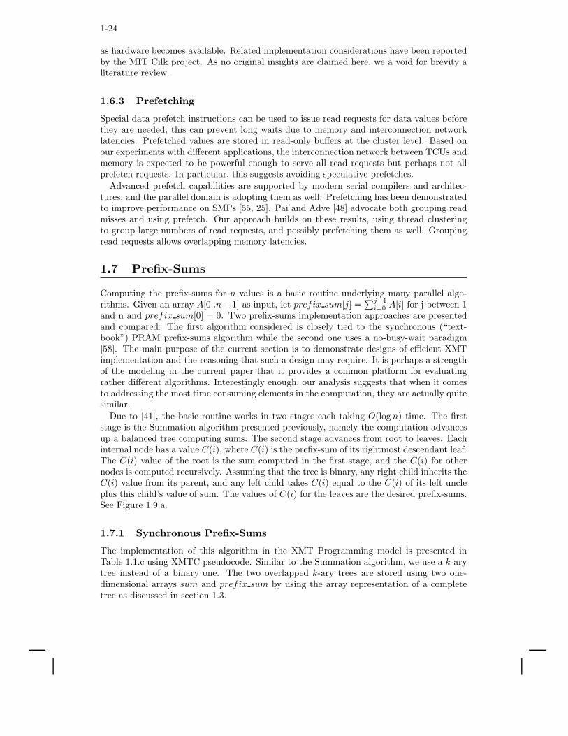
1-24
as hardware becomes available. Related implementation considerations have been reportedby the MIT Cilk project. As no original insights are claimed here, we a void for brevity aliterature review.
1.6.3 Prefetching
Special data prefetch instructions can be used to issue read requests for data values beforethey are needed; this can prevent long waits due to memory and interconnection networklatencies. Prefetched values are stored in read-only buffers at the cluster level. Based onour experiments with different applications, the interconnection network between TCUs andmemory is expected to be powerful enough to serve all read requests but perhaps not allprefetch requests. In particular, this suggests avoiding speculative prefetches.
Advanced prefetch capabilities are supported by modern serial compilers and architec-tures, and the parallel domain is adopting them as well. Prefetching has been demonstratedto improve performance on SMPs [55, 25]. Pai and Adve [48] advocate both grouping readmisses and using prefetch. Our approach builds on these results, using thread clusteringto group large numbers of read requests, and possibly prefetching them as well. Groupingread requests allows overlapping memory latencies.
1.7 Prefix-Sums
Computing the prefix-sums for n values is a basic routine underlying many parallel algo-rithms. Given an array A[0..n− 1] as input, let prefix sum[j] =
∑j−1i=0 A[i] for j between 1
and n and prefix sum[0] = 0. Two prefix-sums implementation approaches are presentedand compared: The first algorithm considered is closely tied to the synchronous (“text-book”) PRAM prefix-sums algorithm while the second one uses a no-busy-wait paradigm[58]. The main purpose of the current section is to demonstrate designs of efficient XMTimplementation and the reasoning that such a design may require. It is perhaps a strengthof the modeling in the current paper that it provides a common platform for evaluatingrather different algorithms. Interestingly enough, our analysis suggests that when it comesto addressing the most time consuming elements in the computation, they are actually quitesimilar.
Due to [41], the basic routine works in two stages each taking O(log n) time. The firststage is the Summation algorithm presented previously, namely the computation advancesup a balanced tree computing sums. The second stage advances from root to leaves. Eachinternal node has a value C(i), where C(i) is the prefix-sum of its rightmost descendant leaf.The C(i) value of the root is the sum computed in the first stage, and the C(i) for othernodes is computed recursively. Assuming that the tree is binary, any right child inherits theC(i) value from its parent, and any left child takes C(i) equal to the C(i) of its left uncleplus this child’s value of sum. The values of C(i) for the leaves are the desired prefix-sums.See Figure 1.9.a.
1.7.1 Synchronous Prefix-Sums
The implementation of this algorithm in the XMT Programming model is presented inTable 1.1.c using XMTC pseudocode. Similar to the Summation algorithm, we use a k-arytree instead of a binary one. The two overlapped k-ary trees are stored using two one-dimensional arrays sum and prefix sum by using the array representation of a completetree as discussed in section 1.3.
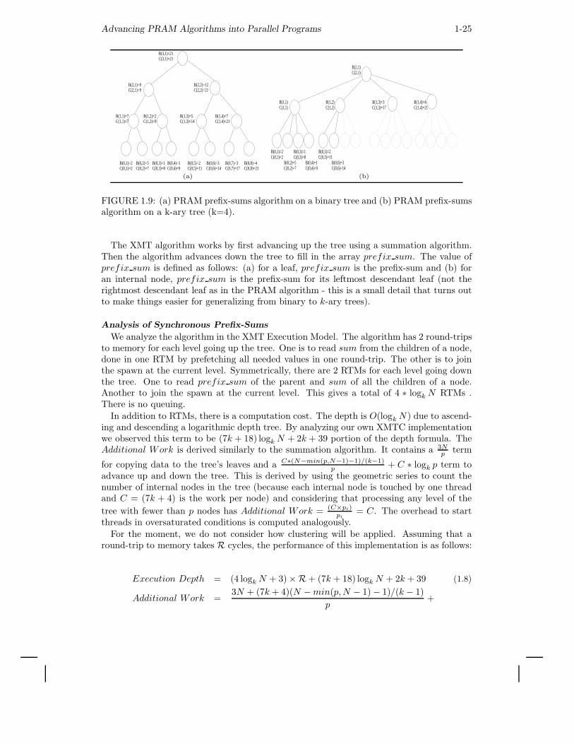
Advancing PRAM Algorithms into Parallel Programs 1-25
C(2,2)=21
B(0,1)=2C(0,1)=2
B(0,2)=5C(0,2)=7
B(0,3)=1C(0,3)=8
B(0,4)=1C(0,4)=9 C(0,5)=11
B(0,5)=2 B(0,6)=3C(0,6)=14
B(0,7)=3C(0,7)=17
B(0,8)=4C(0,8)=21
B(1,1)=7C(1,1)=7
B(2,1)=9C(2,1)=9
B(3,1)=21C(3,1)=21
B(1,4)=7C(1,4)=21
B(1,3)=5C(1,3)=14
B(1,2)=2C(1,2)=9
B(2,2)=12
C(2,1)
B(0,1)=2C(0,1)=2
B(0,2)=5C(0,2)=7
B(0,3)=1C(0,3)=8
B(0,5)=2C(0,5)=11
B(0,4)=1C(0,4)=9
B(0,6)=3C(0,6)=14
B(1,1)C(1,1)
B(1,2)C(1,2)
B(1,3)=3C(1,3)=17
B(1,4)=4C(1,4)=21
B(2,1)
(a) (b)
FIGURE 1.9: (a) PRAM prefix-sums algorithm on a binary tree and (b) PRAM prefix-sumsalgorithm on a k-ary tree (k=4).
The XMT algorithm works by first advancing up the tree using a summation algorithm.Then the algorithm advances down the tree to fill in the array prefix sum. The value ofprefix sum is defined as follows: (a) for a leaf, prefix sum is the prefix-sum and (b) foran internal node, prefix sum is the prefix-sum for its leftmost descendant leaf (not therightmost descendant leaf as in the PRAM algorithm - this is a small detail that turns outto make things easier for generalizing from binary to k-ary trees).
Analysis of Synchronous Prefix-Sums
We analyze the algorithm in the XMT Execution Model. The algorithm has 2 round-tripsto memory for each level going up the tree. One is to read sum from the children of a node,done in one RTM by prefetching all needed values in one round-trip. The other is to jointhe spawn at the current level. Symmetrically, there are 2 RTMs for each level going downthe tree. One to read prefix sum of the parent and sum of all the children of a node.Another to join the spawn at the current level. This gives a total of 4 ∗ logk N RTMs .There is no queuing.
In addition to RTMs, there is a computation cost. The depth is O(logk N) due to ascend-ing and descending a logarithmic depth tree. By analyzing our own XMTC implementationwe observed this term to be (7k + 18) logk N + 2k + 39 portion of the depth formula. TheAdditional Work is derived similarly to the summation algorithm. It contains a 3N
p term
for copying data to the tree’s leaves and a C∗(N−min(p,N−1)−1)/(k−1)p + C ∗ logk p term to
advance up and down the tree. This is derived by using the geometric series to count thenumber of internal nodes in the tree (because each internal node is touched by one threadand C = (7k + 4) is the work per node) and considering that processing any level of the
tree with fewer than p nodes has Additional Work = (C×pi)pi
= C. The overhead to startthreads in oversaturated conditions is computed analogously.
For the moment, we do not consider how clustering will be applied. Assuming that around-trip to memory takes R cycles, the performance of this implementation is as follows:
Execution Depth = (4 logk N + 3) ×R + (7k + 18) logk N + 2k + 39 (1.8)
Additional Work =3N + (7k + 4)(N − min(p, N − 1) − 1)/(k − 1)
p+
1-26
+(7k + 4) logk p +⌈
(N − min(p, N − 1) − 1)/(k − 1)
p− logk
N
p
⌉
× 2R (1.9)
1.7.2 No-Busy-Wait Prefix-Sums
A less-synchronous XMT algorithm is presented. The Synchronous algorithm presentedabove processes each level of the tree before moving to the next, but this algorithm has nosuch restriction. The algorithm is based on the No-Busy-Wait balanced tree paradigm [58].As before, we use k-ary rather than binary trees.
The input and data structures are the same as previously, with the addition of thegatekeeper array, providing a “gatekeeper” variable per tree node. The computation ad-vances up the tree using a No-Busy-Wait summation algorithm. Then it advances downthe tree using a No-Busy-Wait algorithm to fill in the prefix-sums.
The pseudocode of the algorithm in the XMT Programming Model is as follows.
Spawn( f i r s t l e a f , l a s t l e a f )Do whi le a l i v e
Perform psm on parent ’ s gatekeeperI f l a s t to a r r i v e at parent
Move to parent and sum va lue s from ch i l d r enElse
JoinI f at root
Joinpre f ix sum [0 ] = 0 // s e t pre f ix sum o f root to 0Spawn(1 ,1 ) //spawn one thread at the root
Let pre f ix sum va lue o f l e f t c h i l d = pre f ix sum o f parentProceed through ch i l d r en l e f t to r i g h t where each ch i l d i sa s s i gned pre f ix sum va lue equa l to pre f ix sum + sum o f l e f ts i b l i n g Use a nested spawn command to s t a r t a thread tor e c u r s i v e l y handle each ch i l d thread except the l e f tmo s t .Advance to l e f tmo s t ch i l d and repeat .
Analysis of No-Busy-Wait Prefix-Sums
When climbing the tree, the implementation executes 2 RTMs per level, just as in theprevious algorithm. One RTM is to read values of sum from the children, and the other isto use an atomic Prefix-sum instruction on the gatekeeper. The LSRTM to descend the treeis also 2 RTMs per level. First, a thread reads the thread ID assigned to it by the parentthread, in one RTM. The second RTM is used to read prefix sum from the parent and sumfrom the children in order to do the necessary calculations. This is an LSRTM of 4 logk N .Also, there are additional O(1) RTMs. Examining our own XMTC implementation, wehave computed the constants involved.
Queuing is also a factor. In the current algorithm, up to k threads can perform a prefix-sum-to-memory operation concurrently on the same gatekeeper and create a k − 1 queuingdelay (since the first access does not count towards queuing delay). The total QD on thecritical path is (k − 1) logk N .
In addition to RTMs and QD, we count computation depth and work. The computationdepth is O(logk N). Counting the constants our implementation yields (11 +8k) ∗ logk N +
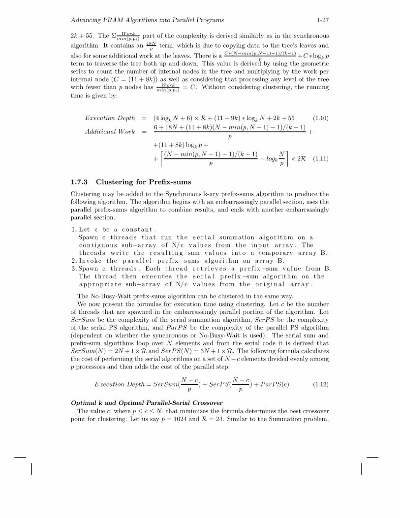
Advancing PRAM Algorithms into Parallel Programs 1-27
2k + 55. The Σ Workmin(p,pi)
part of the complexity is derived similarly as in the synchronous
algorithm. It contains an 18Np term, which is due to copying data to the tree’s leaves and
also for some additional work at the leaves. There is a C∗(N−min(p,N−1)−1)/(k−1)p +C ∗ logk p
term to traverse the tree both up and down. This value is derived by using the geometricseries to count the number of internal nodes in the tree and multiplying by the work perinternal node (C = (11 + 8k)) as well as considering that processing any level of the treewith fewer than p nodes has Work
min(p,pi)= C. Without considering clustering, the running
time is given by:
Execution Depth = (4 logk N + 6) ×R + (11 + 9k) ∗ logk N + 2k + 55 (1.10)
Additional Work =6 + 18N + (11 + 8k)(N − min(p, N − 1) − 1)/(k − 1)
p+
+(11 + 8k) logk p +
+
⌈
(N − min(p, N − 1) − 1)/(k − 1)
p− logk
N
p
⌉
× 2R (1.11)
1.7.3 Clustering for Prefix-sums
Clustering may be added to the Synchronous k-ary prefix-sums algorithm to produce thefollowing algorithm. The algorithm begins with an embarrassingly parallel section, uses theparallel prefix-sums algorithm to combine results, and ends with another embarrassinglyparallel section.
1 . Let c be a constant .Spawn c threads that run the s e r i a l summation a lgor i thm on acont iguous sub−ar ray o f N/c va lue s from the input ar ray . Thethreads wr i t e the r e s u l t i n g sum va lue s in to a temporary ar ray B.
2 . Invoke the p a r a l l e l p r e f i x−sums a lgor i thm on array B.3 . Spawn c threads . Each thread r e t r i e v e s a pr e f i x−sum va lue from B.
The thread then execute s the s e r i a l p r e f i x−sum algor i thm on theappropr i a t e sub−ar ray o f N/c va lue s from the o r i g i n a l a r ray .
The No-Busy-Wait prefix-sums algorithm can be clustered in the same way.We now present the formulas for execution time using clustering. Let c be the number
of threads that are spawned in the embarrassingly parallel portion of the algorithm. LetSerSum be the complexity of the serial summation algorithm, SerPS be the complexityof the serial PS algorithm, and ParPS be the complexity of the parallel PS algorithm(dependent on whether the synchronous or No-Busy-Wait is used). The serial sum andprefix-sum algorithms loop over N elements and from the serial code it is derived thatSerSum(N) = 2N +1×R and SerPS(N) = 3N +1×R. The following formula calculatesthe cost of performing the serial algorithms on a set of N −c elements divided evenly amongp processors and then adds the cost of the parallel step:
Execution Depth = SerSum(N − c
p) + SerPS(
N − c
p) + ParPS(c) (1.12)
Optimal k and Optimal Parallel-Serial Crossover
The value c, where p ≤ c ≤ N , that minimizes the formula determines the best crossoverpoint for clustering. Let us say p = 1024 and R = 24. Similar to the Summation problem,
1-28
we have concluded that in the XMT Execution Model for many values N ≥ p, the best c is1024. This is the case for both algorithms. A different value of c may be optimal for otherapplications, for example if the threads do not have equal work.
The optimal k value, where k denotes the arity of the tree, to use for either of the prefix-sums algorithms can be derived from the formulas. As shown in Figure 1.6.a, for N ≥ p(where p = 1024), the parallel sums algorithm is only run on c = 1024 elements and inthis case k = 8 is optimal for the synchronous algorithm and k = 7 is optimal for theNo-Busy-Wait algorithm. When N < p, clustering does not take effect, and the optimalvalue of k varies with N , for both algorithms.
1.7.4 Comparing Prefix-sums Algorithms
Using the performance model presented previously with these optimizations allows com-parison of the programs in the XMT Execution Model. The execution time for various Nwas calculated for both prefix-sums algorithms using the formula with clustering. This isplotted in Figure 1.6.b.
The Synchronous algorithm performs better, due to the smaller computation constants.The LSRTM of both algorithms is the same, indicating that using gatekeepers and nestingis equivalent in RTMs to using synchronous methods. The No-Busy-Wait algorithm hasslightly longer computation depth and more computation work due to the extra overhead.
We note that in an actual XMT system, an implementation of the Prefix-Sums algorithmwould be likely to be included as a library routine.
1.8 Programming Parallel Breadth-First Search Algorithms
As noted earlier, Breadth-First Search (BFS) provides an interesting example for XMTprogramming. We assume that the graph is provided using the incidence list representation,as pictured in Figure 1.10.a.
Let L(i) be the set of N(i) nodes in level i and E(i) the set of edges adjacent to thesenodes. For brevity, we will only illustrate how to implement one iteration. Developing thefull program based on this is straightforward.
As described in section 1.2.2, the High-Level Work-Depth presentation of the algorithmstarts with all the nodes in parallel, and then using nested parallelism ramps up moreparallelism to traverse all their adjacent edges in one step. Depending on the extent that thetarget programming model supports nested parallelism, the programmer needs to considerdifferent implementations. We discuss these choices in the following paragraphs, laying outassumptions regarding the target XMT model.
We noted before that the Work-Depth model is not a direct match for our proposedprogramming model. With this in mind, we will not present a full Work-Depth descriptionof the BFS algorithm; as will be shown, the “ideal” implementation will be closer to theHigh-Level Work-Depth presentation.
1.8.1 Nested Spawn BFS
In a XMT programming model that supports nested parallel sections, the High-level XMTprogram can be easily derived from the HLWD description:
For every ver tex v o f cur r ent l a y e r L( i ) spawn a threadFor every edge e=(v ,w) adjacent on v spawn a thread
Traverse edge e
Advancing PRAM Algorithms into Parallel Programs 1-29
3 3 1 2 3
3 6 7 90
degree
start_edge
1
5
2
34
1
1
1
2
2
2
2
4
3
5
3 2
4
4
5
5
5
1
5
4
2
1
1
5
3
7
9
0
6
4
1
11
2
5
8
1
2
3
4
6
7
8
9
5
10
11
0
10
antiparalleledges
1 2 3 4 5
������������
������������
������������
������������
������������
������������
������������
������������
b1
b2
b3
b0
v4
v1v2v3
Markeredges
...
w2w1
E(i) level L(i+1)
time
|L(i)| threads p threads
level L(i)
(a) (b)
FIGURE 1.10: (a) The incidence list representation for a graph. (b) Execution of FlattenedBFS algorithm. First allocate E[i] to hold all edges adjacent to level[i]. Next, identifymarker edges bi, which give the first edge per each sub-array. Running one thread persub-array, all edges are traversed to build level[i + 1].
A more detailed implementation of this algorithm using the XMTC programming languageis included in Table 1.1.d. To traverse an edge, threads use an atomic prefix-sum instruc-tion on a special “gatekeeper” memory location associated with the destination node. Allgatekeepers are initially set to 0. Receiving a 0 from the prefix-sum instruction means thethread was the first to reach the destination node. The newly discovered neighbors areadded to layer L(i + 1) using another prefix-sum operation on the size of L(i + 1). In ad-dition, the edge anti-parallel to the one traversed is marked to avoid needlessly traversingit again (in the opposite direction) in later BFS layers. Note that this matches the PRAMArbitrary Concurrent Write convention, as mentioned in section 1.2.3.
The Nested Spawn algorithm bears a natural resemblance to the HLWD presentationof the BFS algorithm and in this sense, is the ideal algorithm to program. Allowing thistype of implementations to be written and efficiently executed is the desired goal of a XMTframework.
Several other XMT BFS algorithms will be presented to demonstrate how BFS couldbe programmed depending on the quantitative and qualitative characteristics of a XMTimplementation.
1.8.2 Flattened BFS
In this algorithm, the total amount of work to process one layer (i.e. the number of edgesadjacent to its vertices) is computed, and it is evenly divided among a pre-determinednumber of threads p, value which depends on architecture parameters. For this, a Prefix-sums subroutine is used to allocate an array of size |E(i)|. The edges will be laid out flatin this array, located contiguously by source vertex. p threads are then spawned, eachbeing assigned one sub-array of |E(i)|/p edges and traversing these edges one by one. Anillustration of the steps in this algorithm can be found in Figure 1.10.b.
To identify the edges in each sub-array, it is sufficient to find the first (called marker)edge in such an interval; we can then use the natural order of the vertices and edges to findthe rest. We start by identifying first (if any) marker edge adjacent to vj for all vertices
1-30
vj ∈ L(i) in parallel, then use a variant of the pointer jumping technique [37, 59] to identifythe rest of the marker edges (if any) adjacent to vj using at most log2 p steps.
1.8.3 Single-spawn and k-spawn BFS
Although the programming model can allow nested parallelism, the execution model mightinclude limited or no support for nesting. To provide insight into the transformations appliedby the compiler, and how to reason about the efficiency of the execution, we present twoimplementations of the Nested Spawn BFS algorithm that directly map into an Executionmodel with limited support for nesting.
The Single-spawn BFS Algorithm uses sspawn() and a binary tree type techniqueto allow the nested spawning of any number T of threads in log2 T steps. The algorithmspawns one thread for each vertex in the current level, and then uses each thread to startdegree(vertex)− 1 additional threads by iteratively using the sspawn() instruction to del-egate half a thread’s work to a new thread. When one edge per thread is reached, the edgesare traversed.
The pseudo-code for a single layer is as follows.
For every ver tex v o f cur r ent l a y e r L spawn a threadWhile a thread needs to handle s > 1 edges
Use sspawn ( ) to s t a r t another thread andde l ega te f l o o r ( s /2 ) edges to i t
Traverse one edge
The k-spawn BFS Algorithm follows the same principle as Single-spawn BFS, but usesthe kspawn() instruction to start the threads faster. By using a k-ary rather than binarytree to emulate the nesting, the number of steps to start T threads is reduced to logk T .
The k-spawn BFS pseudo-code for processing one layer is:
For every ver tex v o f cur r ent l a y e r L spawn a threadWhile a thread needs to handle s > k edges
Use kspawn ( ) to spawn k threads andde l ega te to each f l o o r ( s /(k+1)) edges
Traverse ( at most ) k edges
1.9 Execution of Breadth-First Search Algorithms
In this section, we examine the execution of the Breadth First Search algorithms presented,and analyze the impact compiler optimizations could have on their performance using theXMT Execution Model as a framework to estimate running times.
Flattened BFS
When each of p threads traverses the edges in its sub-array serially, a simple optimizationwould prefetch the next edge data from memory and overlap the prefix-sum operations, thus
reducing the number of round-trips to memory from O( |E(i)|p ) to a small constant. Such an
improvement can be quite significant.The Flattened BFS algorithm uses the prefix sums algorithm as a procedure; we will use
the running time computed for this routine in section 1.7. Analyzing our implementation,we observed that identifying the marker edges uses 3 RTMs to initialize one marker edge
Advancing PRAM Algorithms into Parallel Programs 1-31
per vertex, and then 4 log2 p RTMs to do log2 p rounds of pointer jumping and find the
rest of the adjacent marker edges. Finally, p threads cycle through their subarrays of |E(i)|p
edges. By using the optimizations described above, the only roundtrip to memory penaltiespaid in this step are that of traversing a single edge. A queuing delay occurs at the nodegatekeeper level if several threads reach the same node simultaneously. This delay dependson the structure of the graph, and is denoted GQD in the formula below.
In addition to LSRTM and QD, the computation depth also appears in the depth formula.The 10 log2 p term is the computation depth of the binary tree approach to identifyingmarker edges. The computation depth of the call to prefix-sums is included.
The dominating term of the Additional Work is 7|E(i)|/p + 28N(i)/p, which comes fromthe step at the end of the algorithm in which all the edges are traversed in parallel byp threads, and the new found vertices are added to level L(i + 1). The Additional Workportion of the complexity also contains the work for the call to prefix-sums. The performanceis:
Execution Depth = (4 logk N(i) + 4 log2 p + 14)×R + 38 + 10 log2 p + 7|E(i)/p| +
+16N(i)/p + GQD + Computation Depth(Prefix sums) (1.13)
Additional Work =7|E(i)| + 28N(i) + 15p + 17
p+ ⌈
N(i) − p
p⌉ × R +
+Additional Work(Prefix sums) (1.14)
As before, N(i) is the number of nodes in layer L(i), |E(i)| is the number of edges adjacentto L(i) and R is the number of cycles in one RTM.
The second term of relation 1.14 denotes the overhead of starting additional threads inover-saturated conditions. In the flattened algorithm, this can occur only in the initialphase, when the set of edges E(i) is filled in. To reduce this overhead, we can applyclustering to the relevant parallel sections.
Note the following special case: when the number of edges adjacent to one layer is rela-tively small, there is no need to start p threads to traverse them. We choose a threshold θ,
and if |E(i)|p < θ, then we use p′ = |E(i)|
θ threads. Each will process θ edges. In this case,
the running time is found by taking the formulas above and replacing p with p′ = |E(i)|θ .
Single-spawn BFS
In this algorithm, one thread per each vertex vi is started, and each of these threads thenrepeteadly uses single-spawn to get deg(vi) − 1 threads started.
To estimate the running time of this algorithm, we proceed to enumerate the operationsthat take place on the critical path during the execution:
• Start and initialize the original set of N(i) threads, which in our implementationtakes 3 RTMs to read the vertex data.
• Let dmax be the largest degree among the nodes in current layer. Use single-spawn and log2 dmax iterations to start dmax threads using a balanced binary treeapproach. Starting a new thread at each iteration takes 2 RTMs (as describedin section 1.6.1), summing up 2 log2 dmax RTM on the critical path.
• The final step of traversing edges implies using one prefix-sum instruction on thegatekeeper location and another one to add the vertex to the new layer.
1-32
The cost of queuing at gatekeepers is represented by GQD. In our implementation, thecomputation depth was 18 + 7 log2 dmax.
Up to |E(i)| threads are started using a binary tree, and when this number exceeds thenumber of TCUs p, we account for the additional work and the thread starting overhead.We estimate these delays by following the same reasoning as with the k-ary Summationalgorithm in section 1.3 using a constant of C = 19 cycles work per node as implied by ourimplementation.
The performance is:
Execution Depth = (7 + 2 log2 dmax)R + (18 + 7 log2 dmax) + GQD (1.15)
Additional Work =19(|E(i)| − min(p, |E(i)| − 1) − 1) + 2
p+
+19 log2 |E(i)| +
⌈
|E(i)| − p
p
⌉
×R (1.16)
To avoid starting too many threads, the clustering technique presented in section 1.6.2can be applied. This will reduce the additional work component since the cost of allocatingnew threads to TCUs will no longer be paid for every edge.
k-spawn BFS
The threads are now started using k-ary trees and are therefore shorter. The LSRTM is2 logk dmax. The factor of 2 is due to the 2 RTMs per k-spawn, as per Section 1.6.1.
The computation depth in our XMTC implementation is (5 + 4k) logk dmax. This is anO(k) cost per node, where logk dmax nodes are on the critical path. The queuing cost atthe gatekeepers is denoted by GQD. The Additional Work is computed as in Single-spawnBFS with the constant C = 4k + 3 denoting the work per node in the k-ary tree used tospawn the |E(i)| threads.
The performance is:
Execution Depth = (7 + 2 logk dmax)R + (5 + 4k) logk dmax + 15 + 4k + GQD (1.17)
Additional Work =14|E(i)| + (4k + 3)(|E(i)| − min(p, |E(i)| − 1) − 1)/(k − 1)
p+
+(4k + 3) logk |E(i)| +
⌈
|E(i)| − p
p
⌉
×R (1.18)
Similar to the case of the Single-spawn BFS algorithm, thread clustering can be usedin the k-spawn BFS algorithm by checking the number of virtual threads to determinewhether the k-spawn instruction should continue to be used or if additional spawning is tobe temporarily suspended.
Comparison
We calculated execution time for one iteration (i.e., processing one BFS level) of the BFSalgorithms presented here and the results are depicted in Figure 1.7. This was done for twovalues for the number of vertices N(i) in current level L(i), 500 and 2000. The analysisassumes that all edges with one end in L(i) lead to vertices which have not been visited in aprevious iteration; since there is more work to be done for a “fresh” vertex, this constitutes a
Advancing PRAM Algorithms into Parallel Programs 1-33
worst-case analysis. The same graphs are also used in Section 1.4 for empirically computingspeedups over serial code as we do not see how they could significantly favor a parallelprogram over the serial one. To generate the graphs, we pick a value M and choose thedegrees of the vertices uniformly at random from the range [M/2, 3M/2], which gives atotal number of edges traversed of |E(i)| = M ∗ N(i) on average. Only the total numberof edges is shown in Figure 1.7. We arbitrarily set N(i + 1) = N(i), which gives a queuing
delay at the gatekeepers (GQD) of |E(i)|N(i) = M on average. As stated in section 1.2.5, we
use the value R = 24 for the number of cycles needed for one roundtrip to memory.
For small problems, the k-spawn algorithm came ahead and the Single-spawn one wassecond best. For large problems, the Flattened algorithm performs best, followed by k-spawn and Single-spawn. When the hardware is sub-saturated, the k-spawn and Single-spawn algorithms do best because their depth component is short. These algorithms havean advantage on smaller problem sizes due to their lower constant factors. The k-spawnimplementation performs better than Single-spawn due to the reduced height of the “Spawntree”. The Flattened algorithm has a larger constant factor for the number of RTMS, mostlydue to the introduction of a setup phase which builds and partitions the array of edges.For super-saturated situations, the Flattened algorithm does best due to a smaller workcomponent than the other algorithms.
Note that using the formulas ignores possible gaps in parallel hardware usage. In a highlyunbalanced graph, some nodes have high degree while others have low degree. As manynodes with small degree finish, it may take time before the use of parallel hardware can beramped up again. For example, in the Single-spawn and k-spawn algorithms, the virtualthreads from the small trees can happen to take up all the physical TCUs and prevent thedeep tree from getting started. The small trees may all finish before the deep one starts.This means we are paying the work of doing the small trees plus the depth of the deep tree.A possible workaround would be to label threads according to the amount of work theyneed to accomplish and giving threads with more work a higher priority (e.g. by schedulingthem to start as soon as possible). Note that this issue does not affect the Flattened BFSalgorithm, since the edges in a layer are evenly distributed among the running threads.
1.10 Adaptive Bitonic Sorting
Bilardi and Nicolau’s [9] Adaptive Bitonic Sorting algorithm is discussed next. The keycomponent of this sorting algorithm is a fast, work-optimal merging algorithm based onBatcher’s bitonic network and adapted for shared memory parallel machines. An efficient,general purpose Merge-Sort type algorithm is derived using this merging procedure.
The main advantages of the Bitonic Merging and Sorting algorithms are the small con-stants involved and the fact that they can be implemented on an EREW PRAM. This isan important factor for implementing an algorithm on our proposed XMT model, since itguarantees that no queuing delays will occur. We will only consider the case where theproblem size is N = 2n; the general case is treated in [9]. We note that XMT caters well tothe heavy reliance on pointer manipulation in the algorithm, which tends to be a weaknessfor other parallel architectures.
For conciseness, we focus on presenting the Merging algorithm here. The purpose of thisalgorithm is to take two sorted sequences and merge them into one single sorted sequence.To start, one of the input sequences is reversed and concatenated with the other one. Theresult is what is defined as a bitonic sequence, and it is stored in a bitonic tree - a fullybalanced binary tree of height log2 N whose in-order traversal yields the bitonic sequence,plus an extra node (called spare) to store the Nth element. The goal of the bitonic merging
1-34
algorithm is to transform this tree into a binary tree whose in-order traversal, followed bythe spare node, gives the elements in sorted order.
The key observation of the algorithm is that a single traversal of a bitonic tree from theroot to the leaves is sufficient to have all the elements in the left subtree of the root smallerthan the ones in the right subtree. At each of the log2 N steps of one such traversal, onecomparison is performed, and at most two pairs of values and pointers are exchanged. Afterone such traversal, the algorithm is applied recursively on the left and right children of theroot, and after log2 N rounds (that can be pipelined, as explained below) the leaves arereached and the tree is a binary search tree.
The full description of the algorithm can be found in [9], and can be summarized by thefollowing recursive function, called with the root and spare nodes of the bitonic tree andthe direction of sorting (increasing or decreasing) as arguments:
procedure bimerge ( root , spare , d i r e c t i o n )1 . compare root and spare va lue s to f i nd d i r e c t i o n o f swapping2 . swap root and spare va lue s i f ne c e s sa ry3 . p l = root . l e f t , pr = root . r i g h t4 . whi l e pr not n i l5 . compare pl , pr6 . swap va lue s o f pl , pr and two subt r e e po i n t e r s i f ne c e s sa ry7 . advance pl , pr toward l e a v e s
end8 . in p a r a l l e l run bimerge ( root . l e f t , root ) and
bimerge ( root . r i ght , spare )end
In this algorithm, lines 4-7 traverse the tree from current height to the leaves in O(log N)time. The procedure is called recursively in line 8, starting at the next lowest level of thetree. This leads to an overall time of O(log2 N).
We call stage(k) the set of tree traversals that start at level k (the root being at level 0).There are 2k parallel calls in such a stage. Call phase(0) of a stage the execution of lines1-3 in the above algorithm, and phase(i), i = 1.. log(N) − k − 1 the iterations of lines 4-7.
To obtain a faster algorithm, we note that the traversals of the tree can be pipelined.In general, we can start stage k + 1 as soon as stage k has reached its phase(2). On asynchronous PRAM model, all stages advance at the same speed and thus they will neveroverlap; on a less-asynchronous PRAM implementation, such as PRAM-on-chip, this typeof lockstep execution can be achieved by switching from parallel to serial mode after eachphase. With this modification, the bitonic merging has a running time of O(log N).
We have experimented with two implementations of the Bitonic Merging algorithm:
Pipelined This is an implementation of the O(log N) algorithm that pipelines thestages. We start with an active workset containing only one thread for stage(0)and run one phase at a time, joining threads after one phase is executed. Everyother iteration, we initialize a new stage by adding a corresponding number ofthreads to the active workset. At the same time, the threads that have reachedthe leaves are removed from the workset. When the set of threads is empty, thealgorithm terminates.
Non-pipelined The previous algorithm has a lock-step type execution, with one syn-chronization point after each phase. An implementation with fewer synchroniza-tion points is evaluated, where all phases of a stage are ran in one single parallelsection with no synchronizations, followed by a join command and then the next
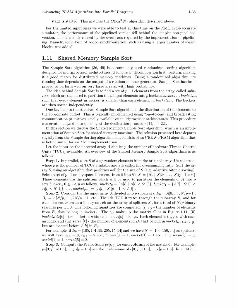
Advancing PRAM Algorithms into Parallel Programs 1-35
stage is started. This matches the O(log2 N) algorithm described above.
For the limited input sizes we were able to test at this time on the XMT cycle-accuratesimulator, the performance of the pipelined version fell behind the simpler non-pipelinedversion. This is mainly caused by the overheads required by the implementation of pipelin-ing. Namely, some form of added synchronization, such as using a larger number of spawnblocks, was added.
1.11 Shared Memory Sample Sort
The Sample Sort algorithm [36, 49] is a commonly used randomized sorting algorithmdesigned for multiprocessor architectures; it follows a “decomposition first” pattern, makingit a good match for distributed memory machines. Being a randomized algorithm, itsrunning time depends on the output of a random number generator. Sample Sort has beenproved to perform well on very large arrays, with high probability.
The idea behind Sample Sort is to find a set of p−1 elements from the array, called split-ters, which are then used to partition the n input elements into p buckets bucket0 . . . bucketp−1
such that every element in bucketi is smaller than each element in bucketi+1. The bucketsare then sorted independently.
One key step in the standard Sample Sort algorithm is the distribution of the elements tothe appropriate bucket. This is typically implemented using “one-to-one” and broadcastingcommunication primitives usually available on multiprocessor architectures. This procedurecan create delays due to queuing at the destination processor [11, 49, 22].
In this section we discuss the Shared Memory Sample Sort algorithm, which is an imple-mentation of Sample Sort for shared memory machines. The solution presented here departsslightly from the Sample Sorting algorithm and consists of an CREW PRAM algorithm thatis better suited for an XMT implementation.
Let the input be the unsorted array A and let p the number of hardware Thread ControlUnits (TCUs) available. An overview of the Shared Memory Sample Sort algorithms is asfollows:
Step 1. In parallel, a set S of s×p random elements from the original array A is collected,where p is the number of TCUs available and s is called the oversampling ratio. Sort the ar-ray S, using an algorithm that performs well for the size of S (e.g. adaptive bitonic sorting).Select a set of p−1 evenly spaced elements from it into S′: S′ = {S[s], S[2s], . . . , S[(p−1)×s]}These elements are the splitters which will be used to partition the elements of A into psets bucketi, 0 ≤ i < p as follows: bucket0 = {A[i] | A[i] < S′[0]}, bucket1 = {A[i] | S′[0] <A[i] < S′[1]}, . . . , bucketp−1 = {A[i] | S′[p − 1] < A[i]}.
Step 2. Consider the the input array A divided into p subarrays, B0 = A[0, . . . , N/p−1],B1 = A[N/p, . . . , 2N/p − 1] etc. The ith TCU iterates through the subarray Bi and foreach element executes a binary search on the array of splitters S′, for a total of N/p binarysearches per TCU. The following quantities are computed: (i) cij - the number of elementsfrom Bi that belong in bucketj. The cij make up the matrix C as in Figure 1.11, (ii)bucket idx[k] - the bucket in which element A[k] belongs. Each element is tagged with suchan index and (iii) serial[k] - the number of elements in Bi that belong in bucketbucket idx[k]
but are located before A[k] in Bi.For example, if B0 = [105, 101, 99, 205, 75, 14] and we have S′ = [100, 150, . . .] as splitters,
we will have c0,0 = 3, c0,1 = 2 etc., bucket[0] = 1, bucket[1] = 1 etc. and serial[0] = 0,serial[1] = 1, serial[5] = 2.
Step 3. Compute the Prefix-Sums ps[i, j] for each column of the matrix C. For example,ps[0, j],ps[1, j],. . . ,ps[p− 1, j] are the prefix-sums of c[0, j],c[1, j],. . . ,c[p− 1, j]. In addition,
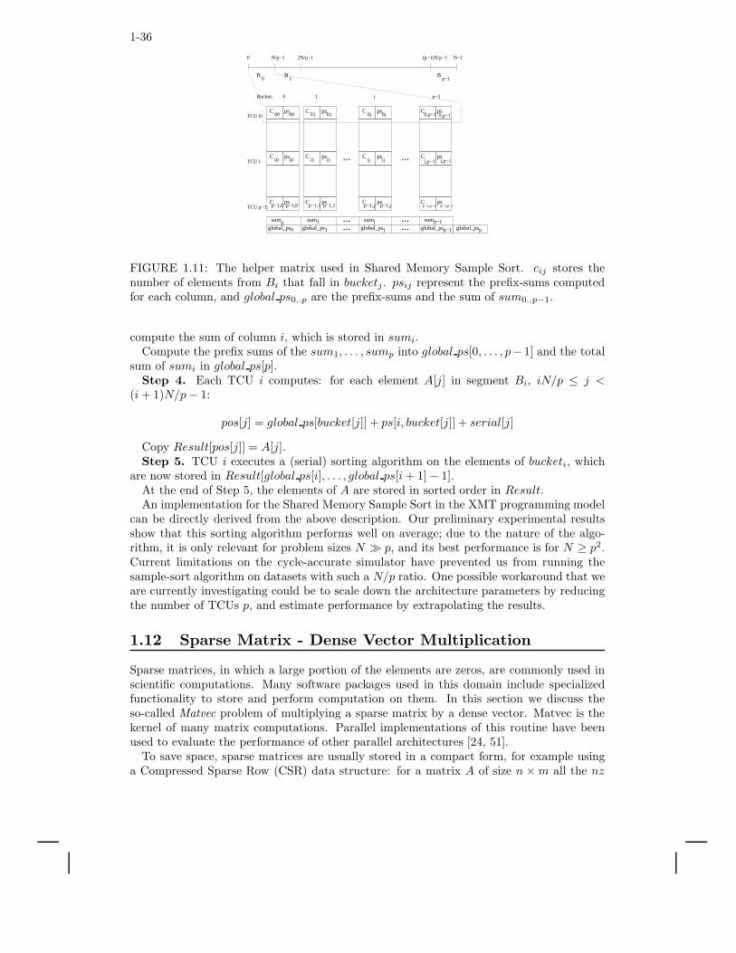
1-36
01
i1
p−1,1
C
C
C psp−1,1
ps01
i1ps
B0
B1
Bp−1
jsumglobal_ps0 global_psj global_psp−1
sum0
sump−1global_psp
sum1global_ps1
... ...
TCU 0:
TCU i:
TCU p−1:
1 j p−10
i,p−1
0,p−1
Bucket:
ij
0jps
ps C
Cps
C00
Ci0
Cp−1,0
psp−1,0
ps
ps
i0
00C
0j
Cij
Cp−1,j p−1,j
C ps0,p−1
psi,p−1
psp−1,p−1 p−1,p−1
N−10 N/p−1 2N/p−1 (p−1)N/p−1
...
.........
FIGURE 1.11: The helper matrix used in Shared Memory Sample Sort. cij stores thenumber of elements from Bi that fall in bucketj. psij represent the prefix-sums computedfor each column, and global ps0..p are the prefix-sums and the sum of sum0..p−1.
compute the sum of column i, which is stored in sumi.Compute the prefix sums of the sum1, . . . , sump into global ps[0, . . . , p− 1] and the total
sum of sumi in global ps[p].Step 4. Each TCU i computes: for each element A[j] in segment Bi, iN/p ≤ j <
(i + 1)N/p − 1:
pos[j] = global ps[bucket[j]] + ps[i, bucket[j]] + serial[j]
Copy Result[pos[j]] = A[j].Step 5. TCU i executes a (serial) sorting algorithm on the elements of bucketi, which
are now stored in Result[global ps[i], . . . , global ps[i + 1] − 1].At the end of Step 5, the elements of A are stored in sorted order in Result.An implementation for the Shared Memory Sample Sort in the XMT programming model
can be directly derived from the above description. Our preliminary experimental resultsshow that this sorting algorithm performs well on average; due to the nature of the algo-rithm, it is only relevant for problem sizes N ≫ p, and its best performance is for N ≥ p2.Current limitations on the cycle-accurate simulator have prevented us from running thesample-sort algorithm on datasets with such a N/p ratio. One possible workaround that weare currently investigating could be to scale down the architecture parameters by reducingthe number of TCUs p, and estimate performance by extrapolating the results.
1.12 Sparse Matrix - Dense Vector Multiplication
Sparse matrices, in which a large portion of the elements are zeros, are commonly used inscientific computations. Many software packages used in this domain include specializedfunctionality to store and perform computation on them. In this section we discuss theso-called Matvec problem of multiplying a sparse matrix by a dense vector. Matvec is thekernel of many matrix computations. Parallel implementations of this routine have beenused to evaluate the performance of other parallel architectures [24, 51].
To save space, sparse matrices are usually stored in a compact form, for example usinga Compressed Sparse Row (CSR) data structure: for a matrix A of size n × m all the nz
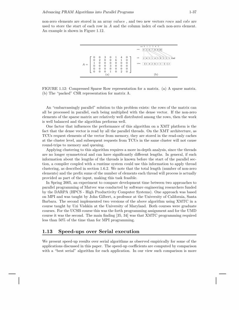
Advancing PRAM Algorithms into Parallel Programs 1-37
non-zero elements are stored in an array values , and two new vectors rows and cols areused to store the start of each row in A and the column index of each non-zero element.An example is shown in Figure 1.12.
A =
0 0 3 0 1 4 00 2 0 0 6 1 01 0 0 0 0 0 00 0 0 3 0 0 00 0 0 0 0 0 00 0 0 1 0 2 0
210 3 4 5row:
rows
cols
values
3 6 7 8 8 10
4
3
2 5 1 4 5 0 3 3 5
1 2 6 1 1 3 1 2
End
0
4
(a) (b)
FIGURE 1.12: Compressed Sparse Row representation for a matrix. (a) A sparse matrix.(b) The “packed” CSR representation for matrix A.
An “embarrassingly parallel” solution to this problem exists: the rows of the matrix canall be processed in parallel, each being multiplied with the dense vector. If the non-zeroelements of the sparse matrix are relatively well distributed among the rows, then the workis well balanced and the algorithm performs well.
One factor that influences the performance of this algorithm on a XMT platform is thefact that the dense vector is read by all the parallel threads. On the XMT architecture, asTCUs request elements of the vector from memory, they are stored in the read-only cachesat the cluster level, and subsequent requests from TCUs in the same cluster will not causeround-trips to memory and queuing.
Applying clustering to this algorithm requires a more in-depth analysis, since the threadsare no longer symmetrical and can have significantly different lengths. In general, if suchinformation about the lengths of the threads is known before the start of the parallel sec-tion, a compiler coupled with a runtime system could use this information to apply threadclustering, as described in section 1.6.2. We note that the total length (number of non-zeroelements) and the prefix sums of the number of elements each thread will process is actuallyprovided as part of the input, making this task feasible.
In Spring 2005, an experiment to compare development time between two approaches toparallel programming of Matvec was conducted by software engineering researchers fundedby the DARPA (HPCS - High Productivity Computer Systems). One approach was basedon MPI and was taught by John Gilbert, a professor at the University of California, SantaBarbara. The second implemented two versions of the above algorithm using XMTC in acourse taught by Uzi Vishkin at the University of Maryland. Both courses were graduatecourses. For the UCSB course this was the forth programming assignment and for the UMDcourse it was the second. The main finding [35, 34] was that XMTC programming requiredless than 50% of the time than for MPI programming.
1.13 Speed-ups over Serial execution
We present speed-up results over serial algorithms as observed empirically for some of theapplications discussed in this paper. The speed-up coefficients are computed by comparisonwith a “best serial” algorithm for each application. In our view such comparison is more
1-38
0 50,000 100,000 150,000 200,000 250,000 300,000 350,000 400,00010
20
30
40
50
60
70
80
90
100
N
Spe
edup
ove
r S
eria
l Pre
fix−
sum
s
SynchronousNo−Busy−WaitSynchronous Linear FitNo−Busy−Wait Linear Fit
0 20,000 40,000 60,000 80,000 100,000 120,000 140,0000
20
40
60
80
100
120
Expected number of edges traversed
Spe
edup
ove
r se
rial v
ersi
on
sspawnflattened
(a) (b)
FIGURE 1.13: (a) Speedup over serial prefix-sums. Due to current limitations of oursimulator we could only run datasets of size up to 200,000. However, fitting a linear curveto the data indicates that the speedups would exceed 100 for problem sizes above 350,000and (b) Speedups of BFS algorithms relative to a serial implementation for N(i) = 500vertices in one BFS level.
useful than comparing with the parallel algorithm run on a single processing unit. In ordernot to give an unfair advantage to the parallel algorithm, we sought to use state-of-the-artcompiler optimizations and architectural features when collecting serial running times. Tothis end, we used the SimpleScalar [14] toolset in the following manner. An “architectureserial speedup coefficient” was computed by running the same serial implementation usingtwo different configurations of the SimpleScalar simulator: (i) one resembling the MasterTCU of the XMT platform, and (ii) one using the most advanced architecture simulatedby SimpleScalar and aggressive compiler optimizations. We computed coefficients for eachapplication and applied them to calibrate all the speedup results.
To obtain the same speedup results using the analytic model, we would have needed topresent a performance model describing a “best serial” architecture and use it to estimaterunning times for the “best serial” algorithm. We considered this to be outside the scopeof this work, and chose to present only experimental speedup results.
Figure 1.13 presents speedup results of parallel Prefix-Sums and Breadth-First Searchimplementations. The XMT architecture simulated included 1024 parallel TCUs groupedinto 64 clusters.
The current paper represents work-in-progress both on the analytic model and on theXMT architecture as a whole. For the future, comparing the outcome of our dry analysiswith the experimental results serves a double purpose: (i) It exposes the strengths andlimitations of the analytic model, allowing further refinements to more closely match thearchitecture. (ii) Proposals for new architecture features can be easily evaluated using theanalytic model and then confirmed in the simulator. This would be more cost-effective thantesting such proposals by committing them to hardware architecture.
1.14 Conclusion
As pointed out earlier, the programming assignments in a one semester parallel algorithmsclass taught recently at the University of Maryland included parallel MATVEC, general
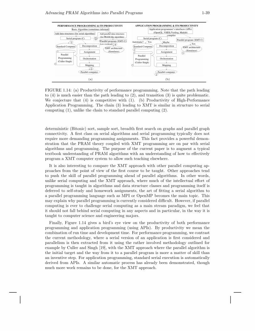
Advancing PRAM Algorithms into Parallel Programs 1-39
(a) (b)
FIGURE 1.14: (a) Productivity of performance programming. Note that the path leadingto (4) is much easier than the path leading to (2), and transition (3) is quite problematic.We conjecture that (4) is competitive with (1). (b) Productivity of High-PerformanceApplication Programming. The chain (3) leading to XMT is similar in structure to serialcomputing (1), unlike the chain to standard parallel computing (2).
deterministic (Bitonic) sort, sample sort, breadth first search on graphs and parallel graphconnectivity. A first class on serial algorithms and serial programming typically does notrequire more demanding programming assignments. This fact provides a powerful demon-stration that the PRAM theory coupled with XMT programming are on par with serialalgorithms and programming. The purpose of the current paper is to augment a typicaltextbook understanding of PRAM algorithms with an understanding of how to effectivelyprogram a XMT computer system to allow such teaching elsewhere.
It is also interesting to compare the XMT approach with other parallel computing ap-proaches from the point of view of the first course to be taught. Other approaches tendto push the skill of parallel programming ahead of parallel algorithms. In other words,unlike serial computing and the XMT approach, where much of the intellectual effort ofprogramming is taught in algorithms and data structure classes and programming itself isdeferred to self-study and homework assignments, the art of fitting a serial algorithm toa parallel programming language such as MPI or OpenMP becomes the main topic. Thismay explain why parallel programming is currently considered difficult. However, if parallelcomputing is ever to challenge serial computing as a main stream paradigm, we feel thatit should not fall behind serial computing in any aspects and in particular, in the way it istaught to computer science and engineering majors.
Finally, Figure 1.14 gives a bird’s eye view on the productivity of both performanceprogramming and application programming (using APIs). By productivity we mean thecombination of run time and development time. For performance programming, we contrastthe current methodology, where a serial version of an application is first considered andparallelism is then extracted from it using the rather involved methodology outlined forexample by Culler and Singh [19], with the XMT approach where the parallel algorithm isthe initial target and the way from it to a parallel program is more a matter of skill thanan inventive step. For application programming, standard serial execution is automaticallyderived from APIs. A similar automatic process has already been demonstrated, thoughmuch more work remains to be done, for the XMT approach.
1-40
Acknowledgments
Contributions and help by the UMD XMT group at and, in particular, N. Ba, A. Balkan,F. Keceli, A. Kupershtok, P. Mazzucco, and X. Wen, as well as the UMD Parallel Algorithmsclass in 2005 and 2006 are gratefully acknowledged.
References
References
[1] A. V. Aho and J. D. Ullman. Foundations of Computer Science. W. H. Freeman &
Co., New York, NY, USA, 1994.
[2] R. Allen, D. Callahan, and K. Kennedy. Automatic decomposition of scientific pro-
grams for parallel execution. In POPL ’87: Proceedings of the 14th ACM SIGACT-SIGPLAN symposium on Principles of programming languages, pages 63–76, New
York, NY, USA, 1987. ACM Press.
[3] G.S. Almasi and A. Gottlieb. Highly Parallel Computing. Benjamin Cummings, 1994.
[4] S. P. Amarasinghe, J. M. Anderson, M. S. Lam, and C. W. Tseng. The suif compiler
for scalable parallel machines. In Proceedings of the Seventh SIAM Conference onParallel Processing for Scientific Computing, 1995.
[5] S. Baase. Computer Algorithms: Introduction to Design and Analysis. Addison-
Wesley, 1988.
[6] D. A. Bader, G. Cong, and J. Feo. On the architectural requirements for efficient
execution of graph algorithms. In ICPP ’05: Proceedings of the 2005 Interna-tional Conference on Parallel Processing (ICPP’05), pages 547–556, Washington,
DC, USA, 2005. IEEE Computer Society.
[7] A. Balkan, G. Qu, and U. Vishkin. Mesh-of-trees and alternative interconnection
networks for single-chip parallel processing. In ASAP 2006: 17th IEEE InternationConference on Application-specific Systems, Architectures and Processors, pages
73–80, Steamboat Springs, Colorado, 2006. Best Paper Award.
[8] A. O. Balkan and U. Vishkin. Programmer’s manual for xmtc language, xmtc compiler
and xmt simulator. Technical Report UMIACS-TR 2005-45, University of Maryland
Institute for Advanced Computer Studies (UMIACS), February 2006.
[9] G. Bilardi and A. Nicolau. Adaptive bitonic sorting: an optimal parallel algorithm for
shared-memory machines. SIAM J. Comput., 18(2):216–228, 1989.
[10] G. E. Blelloch. Programming parallel algorithms. Commun. ACM, 39(3):85–97, 1996.
[11] G. E. Blelloch, C. E. Leiserson, B. M. Maggs, C. G. Plaxton, S. J. Smith, and M. Za-
gha. A comparison of sorting algorithms for the connection machine cm-2. In SPAA’91: Proceedings of the third annual ACM symposium on Parallel algorithms andarchitectures, pages 3–16, New York, NY, USA, 1991. ACM Press.
[12] R.D. Blumofe and C. E. Leiserson. Space-efficient scheduling of multithreaded com-
putations. In 25th Annual ACM Symposium on the Theory of Computing (STOC’93), pages 362–371, 1993.
[13] R. P. Brent. The parallel evaluation of general arithmetic expressions. J. ACM,
21(2):201–206, 1974.
[14] D. Burger and T. M. Austin. The simplescalar tool set, version 2.0. SIGARCHComput. Archit. News, 25(3):13–25, 1997.
[15] L. Carter, J. Feo, and A. Snavely. Performance and programming experience on the
tera mta. In Proceedings SIAM Conference on Parallel Processing, 1999.
[16] R. Cole and U. Vishkin. Deterministic coin tossing and accelerating cascades: micro
Advancing PRAM Algorithms into Parallel Programs 1-41
and macro techniques for designing parallel algorithms. In STOC ’86: Proceedingsof the eighteenth annual ACM symposium on Theory of computing, pages 206–219,
New York, NY, USA, 1986. ACM Press.
[17] R. Cole and O. Zajicek. The apram: incorporating asynchrony into the pram model. In
SPAA ’89: Proceedings of the first annual ACM symposium on Parallel algorithmsand architectures, pages 169–178, New York, NY, USA, 1989. ACM Press.
[18] T. H. Cormen, C. E. Leiserson, and R. L. Rivest. Introduction to Algorithms. MIT
Press, first edition, 1990.
[19] D. E. Culler and J. P. Singh. Parallel Computer Architecture: A Hardware/SoftwareApproach. Morgan Kaufmann Publishers Inc., San Francisco, CA, USA, 1999.
[20] S. Dascal and U. Vishkin. Experiments with list ranking for explicit multi-threaded
(xmt) instruction parallelism. J. Exp. Algorithmics, 5:10, 2000. Special issue for the
3rd Workshop on Algorithms Engineering (WAE’99), London, U.K., July 1999.
[21] R. Dementiev, M. Klein, and W. J. Paul. Performance of mp3d on the sb-pram
prototype (research note). In Euro-Par ’02: Proceedings of the 8th InternationalEuro-Par Conference on Parallel Processing, pages 132–136, London, UK, 2002.
Springer-Verlag.
[22] A. C. Dusseau, D. E. Culler, K. E. Schauser, and R. P. Martin. Fast parallel sorting
under logp: Experience with the cm-5. IEEE Trans. Parallel Distrib. Syst., 7(8):791–
805, 1996.
[23] D. Eppstein and Z. Galil. Parallel algorithmic techniques for combinatorial computa-
tion. Annual review of computer science: vol. 3, 1988, pages 233–283, 1988.
[24] J. Feo, D. Harper, S. Kahan, and P. Konecny. Eldorado. In CF ’05: Proceedingsof the 2nd conference on Computing frontiers, pages 28–34, New York, NY, USA,
2005. ACM Press.
[25] M. J. Garzaran, J. L. Briz, P. Ibanez, and V. Vinals. Hardware prefetching in bus-based
multiprocessors: pattern characterization and cost-effective hardware. In Proceedingsof the Euromicro Workshop on Parallel and Distributed Processing, pages 345–354,
2001.
[26] P. B. Gibbons. A more practical pram model. In SPAA ’89: Proceedings of the firstannual ACM symposium on Parallel algorithms and architectures, pages 158–168,
New York, NY, USA, 1989. ACM Press.
[27] P. B. Gibbons, Y. Matias, and V. Ramachandran. The queue-read queue-write asyn-
chronous pram model. Theor. Comput. Sci., 196(1-2):3–29, 1998.
[28] A. Gottlieb, R. Grishman, C. P. Kruskal, K. P. McAuliffe, L. Rudolph, and M. Snir.
The nyu ultracomputer: designing a mimd, shared-memory parallel machine (extended
abstract). In ISCA ’82: Proceedings of the 9th annual symposium on ComputerArchitecture, pages 27–42, Los Alamitos, CA, USA, 1982. IEEE Computer Society
Press.
[29] A. Gress and G. Zachmann. Gpu-bisort: Optimal parallel sorting on stream archi-
tectures. In IPDPS ’06: Proceedings of the 20th IEEE International Parallel andDistributed Processing Symposium (IPDPS’06), 2006. To appear.
[30] P. Gu and U. Vishkin. Case study of gate-level logic simulation on an extermely
fine-grained chip multiprocessor. Journal of Embedded Computing, Special Issue onEmbedded Single-Chip Multicore Architectures and Related Research - from SystemDesign to Application Support, 2006. To appear.
[31] M. J. Harris, W. V. Baxter, T. Scheuermann, and A. Lastra. Simulation of cloud
dynamics on graphics hardware. In HWWS ’03: Proceedings of the ACM SIG-GRAPH/EUROGRAPHICS conference on Graphics hardware, pages 92–101, Aire-
la-Ville, Switzerland, Switzerland, 2003. Eurographics Association.
1-42
[32] D. R. Helman and J. JaJa. Designing practical efficient algorithms for symmetric
multiprocessors. In ALENEX ’99: Selected papers from the International Workshopon Algorithm Engineering and Experimentation, pages 37–56, London, UK, 1999.
Springer-Verlag.
[33] J. L. Hennessy and D. A. Patterson. Computer Architecture: A Quantitative Ap-proach. Morgan Kaufmann Publishers Inc., San Francisco, CA, USA, 2003.
[34] L. Hochstein and V. R. Basili. An empirical study to compare two parallel program-
ming models. 18th ACM Symposium on Parallelism in Algorithms and Architec-tures (SPAA ’06), July 2006. Position Paper and Brief Announcement.
[35] L. Hochstein, U. Vishkin, J. Gilbert, and V. Basili. An empirical study to compare
the productivity of two parallel programming models. Preprint, 2005.
[36] J.S. Huang and Y.C. Chow. Parallel sorting and data partitioning by sampling. In
Proceedings of the IEEE Computer Society’s Seventh International Computer Soft-ware and Applications Conference, pages 627–631, November 1983.
[37] J. JaJa. An introduction to parallel algorithms. Addison Wesley Longman Publishing
Co., Inc., Redwood City, CA, USA, 1992.
[38] R. M. Karp and V. Ramachandran. Parallel algorithms for shared-memory machines.
Handbook of theoretical computer science (vol. A): algorithms and complexity,pages 869–941, 1990.
[39] J. Keller, C. W. Kessler, and J. L. Traff. Practical PRAM Proramming. Wiley, New
York, NY, USA, 2000.
[40] P. Kipfer, M. Segal, and R. Westermann. Uberflow: a gpu-based particle engine. In
HWWS ’04: Proceedings of the ACM SIGGRAPH/EUROGRAPHICS conferenceon Graphics hardware, pages 115–122, New York, NY, USA, 2004. ACM Press.
[41] R. E. Ladner and M. J. Fischer. Parallel prefix computation. J. ACM, 27(4):831–838,
1980.
[42] C.E. Leiserson and H. Prokop. Minicourse on multithreaded programming.
http://supertech.csail.mit.edu/cilk/papers/index.html, 1998.
[43] U. Manber. Introduction to Algorithms - A Creative Approach. Addison Wesley,
1989.
[44] K. Moreland and E. Angel. The fft on a gpu. In HWWS ’03: Proceedings of the ACMSIGGRAPH/EUROGRAPHICS conference on Graphics hardware, pages 112–119,
Aire-la-Ville, Switzerland, Switzerland, 2003. Eurographics Association.
[45] D. Naishlos, J. Nuzman, C-W. Tseng, and U. Vishkin. Evaluating multi-threading
in the prototype xmt environment. In Proceedings 4th Workshop on MultithreadedExecution, Architecture, and Compilation, 2000.
[46] D. Naishlos, J. Nuzman, C-W. Tseng, and U. Vishkin. Evaluating the xmt program-
ming model. In Proceedings of the 6th Workshop on High-level Parallel Program-ming Models and Supportive Environments, pages 95–108, 2001.
[47] D. Naishlos, J. Nuzman, C-W. Tseng, and U. Vishkin. Towards a first vertical proto-
typing of an extremely fine-grained parallel programming approach. In invited SpecialIssue for ACM-SPAA’01: TOCS 36,5, pages 521–552, New York, NY, USA, 2003.
Springer Verlag.
[48] V. S. Pai and S. V. Adve. Comparing and combining read miss clustering and soft-
ware prefetching. In PACT ’01: Proceedings of the 2001 International Conferenceon Parallel Architectures and Compilation Techniques, page 292, Washington, DC,
USA, 2001. IEEE Computer Society.
[49] J. H. Reif and L. G. Valiant. A logarithmic time sort for linear size networks. J. ACM,
34(1):60–76, 1987.
[50] J. T. Schwartz. Ultracomputers. ACM Trans. Program. Lang. Syst., 2(4):484–521,
Advancing PRAM Algorithms into Parallel Programs 1-43
1980.
[51] V. Shah and J. R. Gilbert. Sparse matrices in matlab*p: Design and implementation.
In HiPC, pages 144–155, 2004.
[52] Y. Shiloach and U. Vishkin. An o(n2logn) parallel max-flow algorithm. J. Algorithms,3(2):128–146, 1982.
[53] S. Skiena. The Algorithm Design Manual. Springer, Nov 1997.
[54] A. Snavely, L. Carter, J. Boisseau, A. Majumdar, K. S. Gatlin, N. Mitchell, J. Feo, and
B. Koblenz. Multi-processor performance on the tera mta. In Supercomputing ’98:Proceedings of the 1998 ACM/IEEE conference on Supercomputing (CDROM),pages 1–8, Washington, DC, USA, 1998. IEEE Computer Society.
[55] X. Tian, R. Krishnaiyer, H. Saito, M. Girkar, and W. Li. Impact of compiler-based
data-prefetching techniques on spec omp application performance. In IPDPS ’05:Proceedings of the 19th IEEE International Parallel and Distributed ProcessingSymposium (IPDPS’05) - Papers, page 53.1, Washington, DC, USA, 2005. IEEE
Computer Society.
[56] A. Tzannes, R. Barua, G.C. Caragea, and U. Vishkin. Issues in writing a parallel
compiler starting from a serial compiler. Draft, 2006.
[57] U. Vishkin. From algorithm parallelism to instruction-level parallelism: an encode-
decode chain using prefix-sum. In SPAA ’97: Proceedings of the 9th annual ACMsymposium on Parallel algorithms and architectures, pages 260–271, New York, NY,
USA, 1997. ACM Press.
[58] U. Vishkin. A no-busy-wait balanced tree parallel algorithmic paradigm. In SPAA’00: Proceedings of the twelfth annual ACM symposium on Parallel algorithms andarchitectures, pages 147–155, New York, NY, USA, 2000. ACM Press.
[59] U. Vishkin. Thinking in parallel: Some basic data-parallel algorithms and techniques.
In use as class notes since 1993. http://www.umiacs.umd.edu/users/vishkin/
PUBLICATIONS/classnotes.ps, February 2002.
[60] U. Vishkin, S. Dascal, E. Berkovich, and J. Nuzman. Explicit multi-threading (xmt)
bridging models for instruction parallelism (extended abstract). In SPAA ’98: Pro-ceedings of the tenth annual ACM symposium on Parallel algorithms and archi-tectures, pages 140–151, New York, NY, USA, 1998. ACM Press.
[61] X. Wen and U. Vishkin. Pram-on-chip: First commitment to silicon. In preparation,
2007.
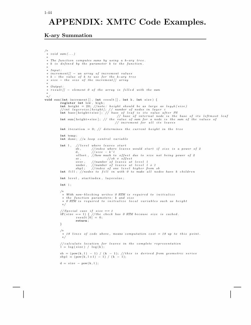
1-44
APPENDIX: XMTC Code Examples.
K-ary Summation
/∗∗ void sum ( . . . )∗∗ The funct ion computes sums by using a k−ary t re e .∗ k i s de f ined by the parameter k to the funct ion .∗∗ Input :∗ increment [ ] − an array of increment va lues∗ k − the va lue of k to use for the k−ary t re e∗ s i z e − the s i z e of the increment [ ] array∗∗ Output :∗ r e s u l t [ ] − element 0 of the array i s f i l l e d with the sum∗∗/
void sum( int increment [ ] , int r e s u l t [ ] , int k , int s i z e ) {register int low , high ;int he ight = 20 ; //note : he igh t should be as l a rg e as l o g k ( s i z e )// in t l a y e r s i z e [ he igh t ] ; / / number of nodes in laye r iint base [ he ight ∗ s i z e ] ; // base of l e a f i s i t s va lue a f t e r PS
// base of in t e rna l node i s the base of i t s l e f tmos t l e a fint sum [ he ight∗ s i z e ] ; // the va lue of sum for a node i s the sum of the va lues of
// increment for a l l i t s l e ave s
int i t e r a t i o n = 0 ; // determines the current he igh t in the t re e
int temp ;int done ; //a loop contro l var iab l e
int l , // l e v e l where l eave s s t a r tsb , // index where l eave s would s t a r t i f s i z e i s a power of 2d , // s i z e − kˆ lo f f s e t , //how much to o f f s e t due to s i z e not being power of 2sr , // sb + o f f s e tover , //number of l e ave s at l e v e l lunder , //number of l e ave s at l e v e l l + 1sbp1 ; // index of one l e v e l h igher from sb
int f i l l ; //nodes to f i l l in with 0 to make a l l nodes have k ch i l d ren
int l e v e l , s t a r t i ndex , l a y e r s i z e ;
int i ;
/∗∗ With non−b l ock ing wr i t e s 0 RTM is required to i n i t i a l i z e∗ the funct ion parameters : k and s i z e∗ 0 RTM is required to i n i t i a l i z e l o c a l v a r i a b l e s such as he igh t∗/
//Spec ia l case i f s i z e == 1i f ( s i z e == 1) { // the check has 0 RTM because s i z e i s cached .
r e s u l t [ 0 ] = 0 ;return ;
}
/∗∗ 18 l i n e s of code above , means computation cost = 18 up to t h i s point .∗/
// c a l c u l a t e l oca t ion for l eave s in the complete representat ionl = l og ( s i z e ) / l og (k ) ;
sb = (pow(k , l ) − 1 ) / ( k − 1 ) ; // t h i s i s der ived from geometric s e r i e ssbp1 = (pow(k , l +1) − 1) / ( k − 1) ;
d = s i z e − pow(k , l ) ;
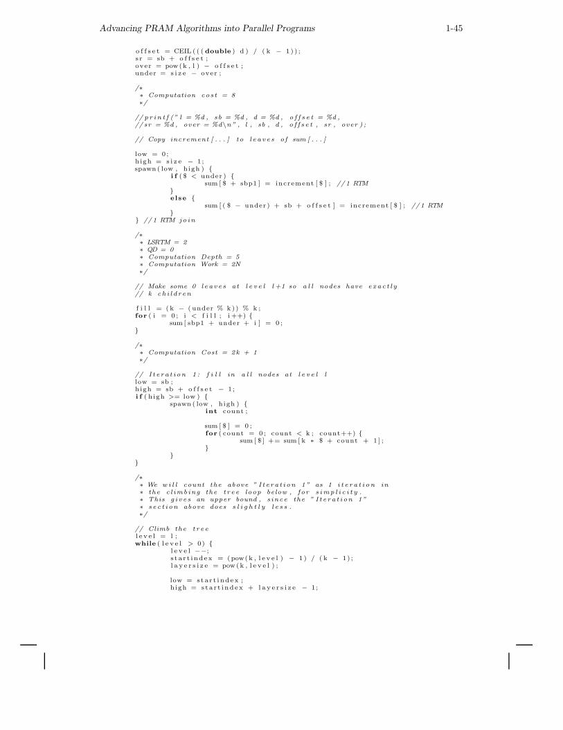
Advancing PRAM Algorithms into Parallel Programs 1-45
o f f s e t = CEIL ( ( ( double ) d ) / ( k − 1 ) ) ;s r = sb + o f f s e t ;over = pow(k , l ) − o f f s e t ;under = s i z e − over ;
/∗∗ Computation cost = 8∗/
// p r in t f (” l = %d , sb = %d , d = %d , o f f s e t = %d ,// sr = %d , over = %d\n” , l , sb , d , o f f s e t , sr , over ) ;
// Copy increment [ . . . ] to l eave s of sum [ . . . ]
low = 0;high = s i z e − 1;spawn ( low , high ) {
i f ( $ < under ) {sum [ $ + sbp1 ] = increment [ $ ] ; //1 RTM
}else {
sum [ ( $ − under ) + sb + o f f s e t ] = increment [ $ ] ; //1 RTM}
} //1 RTM jo in
/∗∗ LSRTM = 2∗ QD = 0∗ Computation Depth = 5∗ Computation Work = 2N∗/
// Make some 0 l eave s at l e v e l l +1 so a l l nodes have exac t l y// k ch i l d ren
f i l l = ( k − ( under % k )) % k ;for ( i = 0 ; i < f i l l ; i ++) {
sum [ sbp1 + under + i ] = 0 ;}
/∗∗ Computation Cost = 2k + 1∗/
// I t e ra t ion 1 : f i l l in a l l nodes at l e v e l llow = sb ;high = sb + o f f s e t − 1;i f ( high >= low ) {
spawn ( low , high ) {int count ;
sum [ $ ] = 0 ;for ( count = 0 ; count < k ; count++) {
sum [ $ ] += sum [ k ∗ $ + count + 1 ] ;}
}}
/∗∗ We w i l l count the above ” I t e ra t ion 1” as 1 i t e r a t i on in∗ the c l imbing the t re e loop below , for s imp l i c i t y .∗ This g iv e s an upper bound , s ince the ” I t e ra t ion 1”∗ se c t ion above does s l i g h t l y l e s s .∗/
// Climb the t re el e v e l = l ;while ( l e v e l > 0) {
l e v e l −−;s t a r t i ndex = (pow(k , l e v e l ) − 1 ) / ( k − 1) ;l a y e r s i z e = pow(k , l e v e l ) ;
low = sta r t i ndex ;high = sta r t i ndex + l a y e r s i z e − 1;
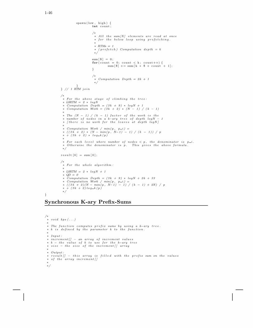
1-46
spawn ( low , high ) {int count ;
/∗∗ Al l the sum[X] elements are read at once∗ for the below loop using pre fe t ch ing .∗∗ RTMs = 1∗ ( pre fe t ch ) Computation depth = k∗/
sum [ $ ] = 0 ;for ( count = 0 ; count < k ; count++) {
sum [ $ ] += sum [ k ∗ $ + count + 1 ] ;}
/∗∗ Computation Depth = 2k + 1∗/
}} // 1 RTM jo in
/∗∗ For the above stage of c l imbing the t re e :∗ LSRTM = 2 ∗ logN∗ Computation Depth = (3k + 9) ∗ logN + 1∗ Computation Work = (3k + 2) ∗ (N − 1) / ( k − 1)∗∗ The (N − 1) / ( k − 1) fac tor of the work i s the∗ number of nodes in a k−ary t re e of depth logN − 1∗ [ there i s no work for the l eave s at depth logN ]∗∗ Computation Work / min(p , p i ) =∗ ((3 k + 2) ∗ (N − min(p , N−1) − 1) / ( k − 1)) / p∗ + (3k + 2) ∗ l o g k (p)∗∗ For each l e v e l where number of nodes < p , the denominator i s p i .∗ Otherwise the denominator i s p . This g iv e s the above formula .∗/
r e s u l t [ 0 ] = sum [ 0 ] ;
/∗∗ For the whole algorithm :∗∗ LSRTM = 2 ∗ logN + 1∗ QD = 0∗ Computation Depth = (3k + 9) ∗ logN + 2k + 33∗ Computation Work / min(p , p i ) =∗ ((3 k + 2)(N − min(p , N−1) − 1) / ( k − 1) + 2N) / p∗ + (3k + 2) lo g k (p)∗/
}
Synchronous K-ary Prefix-Sums
/∗∗ void kps ( . . . )∗∗ The funct ion computes p r e f i x sums by using a k−ary t re e .∗ k i s de f ined by the parameter k to the funct ion .∗∗ Input :∗ increment [ ] − an array of increment va lues∗ k − the va lue of k to use for the k−ary t re e∗ s i z e − the s i z e of the increment [ ] array∗∗ Output :∗ r e s u l t [ ] − t h i s array i s f i l l e d with the p r e f i x sum on the va lues∗ of the array increment [ ]∗∗/
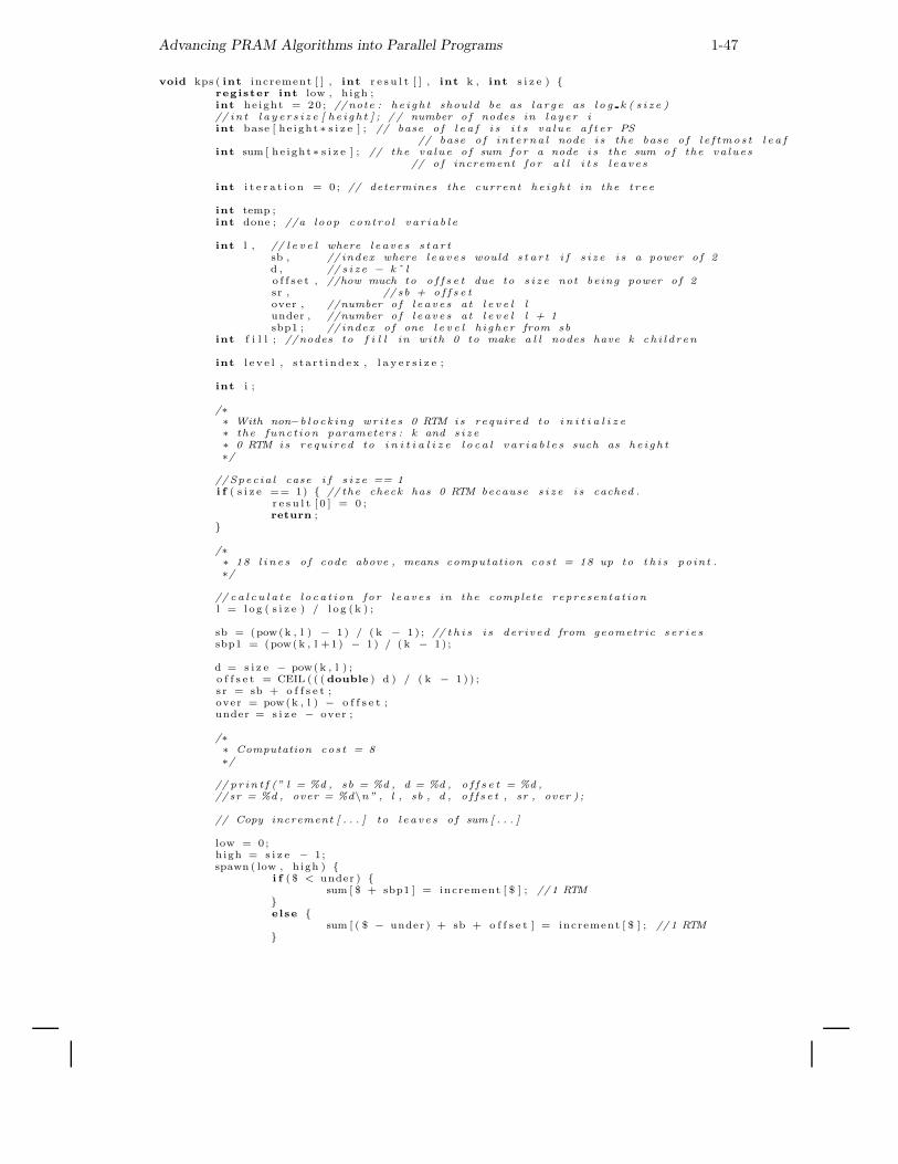
Advancing PRAM Algorithms into Parallel Programs 1-47
void kps ( int increment [ ] , int r e s u l t [ ] , int k , int s i z e ) {register int low , high ;int he ight = 20 ; //note : he igh t should be as l a rg e as l o g k ( s i z e )// in t l a y e r s i z e [ he igh t ] ; / / number of nodes in laye r iint base [ he ight ∗ s i z e ] ; // base of l e a f i s i t s va lue a f t e r PS
// base of in t e rna l node i s the base of l e f tmos t l e a fint sum [ he ight∗ s i z e ] ; // the va lue of sum for a node i s the sum of the va lues
// of increment for a l l i t s l e ave s
int i t e r a t i o n = 0 ; // determines the current he igh t in the t re e
int temp ;int done ; //a loop contro l var iab l e
int l , // l e v e l where l eave s s t a r tsb , // index where l eave s would s t a r t i f s i z e i s a power of 2d , // s i z e − kˆ lo f f s e t , //how much to o f f s e t due to s i z e not being power of 2sr , // sb + o f f s e tover , //number of l e ave s at l e v e l lunder , //number of l e ave s at l e v e l l + 1sbp1 ; // index of one l e v e l h igher from sb
int f i l l ; //nodes to f i l l in with 0 to make a l l nodes have k ch i l d ren
int l e v e l , s t a r t i ndex , l a y e r s i z e ;
int i ;
/∗∗ With non−b l ock ing wr i t e s 0 RTM is required to i n i t i a l i z e∗ the funct ion parameters : k and s i z e∗ 0 RTM is required to i n i t i a l i z e l o c a l v a r i a b l e s such as he igh t∗/
//Spec ia l case i f s i z e == 1i f ( s i z e == 1) { // the check has 0 RTM because s i z e i s cached .
r e s u l t [ 0 ] = 0 ;return ;
}
/∗∗ 18 l i n e s of code above , means computation cost = 18 up to t h i s point .∗/
// c a l c u l a t e l oca t ion for l eave s in the complete representat ionl = l og ( s i z e ) / l og (k ) ;
sb = (pow(k , l ) − 1 ) / ( k − 1 ) ; // t h i s i s der ived from geometric s e r i e ssbp1 = (pow(k , l +1) − 1) / ( k − 1) ;
d = s i z e − pow(k , l ) ;o f f s e t = CEIL ( ( ( double ) d ) / ( k − 1 ) ) ;s r = sb + o f f s e t ;over = pow(k , l ) − o f f s e t ;under = s i z e − over ;
/∗∗ Computation cost = 8∗/
// p r in t f (” l = %d , sb = %d , d = %d , o f f s e t = %d ,// sr = %d , over = %d\n” , l , sb , d , o f f s e t , sr , over ) ;
// Copy increment [ . . . ] to l eave s of sum [ . . . ]
low = 0;high = s i z e − 1;spawn ( low , high ) {
i f ( $ < under ) {sum [ $ + sbp1 ] = increment [ $ ] ; //1 RTM
}else {
sum [ ( $ − under ) + sb + o f f s e t ] = increment [ $ ] ; //1 RTM}
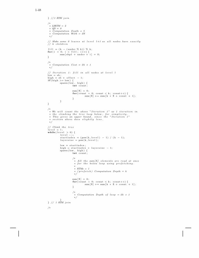
1-48
} //1 RTM jo in
/∗∗ LSRTM = 2∗ QD = 0∗ Computation Depth = 5∗ Computation Work = 2N∗/
// Make some 0 l eave s at l e v e l l +1 so a l l nodes have exac t l y// k ch i l d ren
f i l l = ( k − ( under % k )) % k ;for ( i = 0 ; i < f i l l ; i ++) {
sum [ sbp1 + under + i ] = 0 ;}
/∗∗ Computation Cost = 2k + 1∗/
// I t e ra t ion 1 : f i l l in a l l nodes at l e v e l llow = sb ;high = sb + o f f s e t − 1;i f ( high >= low ) {
spawn ( low , high ) {int count ;
sum [ $ ] = 0 ;for ( count = 0 ; count < k ; count++) {
sum [ $ ] += sum [ k ∗ $ + count + 1 ] ;}
}}
/∗∗ We w i l l count the above ” I t e ra t ion 1” as 1 i t e r a t i on in∗ the c l imbing the t re e loop below , for s imp l i c i t y .∗ This g iv e s an upper bound , s ince the ” I t e ra t ion 1”∗ se c t ion above does s l i g h t l y l e s s .∗/
// Climb the t re el e v e l = l ;while ( l e v e l > 0) {
l e v e l −−;s t a r t i ndex = (pow(k , l e v e l ) − 1 ) / ( k − 1) ;l a y e r s i z e = pow(k , l e v e l ) ;
low = sta r t i ndex ;high = sta r t i ndex + l a y e r s i z e − 1;spawn ( low , high ) {
int count ;
/∗∗ Al l the sum[X] elements are read at once∗ for the below loop using pre fe t ch ing .∗∗ RTMs = 1∗ ( pre fe t ch ) Computation Depth = k∗/
sum [ $ ] = 0 ;for ( count = 0 ; count < k ; count++) {
sum [ $ ] += sum [ k ∗ $ + count + 1 ] ;}
/∗∗ Computation Depth of loop = 2k + 1∗/
}} // 1 RTM jo in
/∗
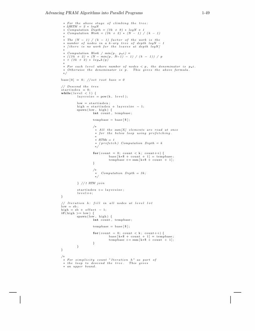
Advancing PRAM Algorithms into Parallel Programs 1-49
∗ For the above stage of c l imbing the t re e :∗ LSRTM = 2 ∗ logN∗ Computation Depth = (3k + 9) ∗ logN + 1∗ Computation Work = (3k + 2) ∗ (N − 1) / ( k − 1)∗∗ The (N − 1) / ( k − 1) fac tor of the work i s the∗ number of nodes in a k−ary t re e of depth logN − 1∗ [ there i s no work for the l eave s at depth logN ]∗∗ Computation Work / min(p , p i ) =∗ ((3 k + 2) ∗ (N − min(p , N−1) − 1) / ( k − 1)) / p∗ + (3k + 2) ∗ l o g k (p)∗∗ For each l e v e l where number of nodes < p , the denominator i s p i .∗ Otherwise the denominator i s p . This g iv e s the above formula .∗/
base [ 0 ] = 0 ; // se t root base = 0
// Descend the t re es t a r t i ndex = 0;while ( l e v e l < l ) {
l a y e r s i z e = pow(k , l e v e l ) ;
low = sta r t i ndex ;high = sta r t i ndex + l a y e r s i z e − 1;spawn ( low , high ) {
int count , tempbase ;
tempbase = base [ $ ] ;
/∗∗ Al l the sum[X] elements are read at once∗ for the below loop using pre fe t ch ing .∗∗ RTMs = 1∗ ( pre fe t ch ) Computation Depth = k∗/
for ( count = 0 ; count < k ; count++) {base [ k∗$ + count + 1] = tempbase ;tempbase += sum [ k∗$ + count + 1 ] ;
}
/∗∗ Computation Depth = 3k ;∗/
} //1 RTM jo in
s t a r t i ndex += l a y e r s i z e ;l e v e l++;
}
// I t e ra t ion h : f i l l in a l l nodes at l e v e l l+1low = sb ;high = sb + o f f s e t − 1;i f ( high >= low ) {
spawn ( low , high ) {int count , tempbase ;
tempbase = base [ $ ] ;
for ( count = 0 ; count < k ; count++) {base [ k∗$ + count + 1] = tempbase ;tempbase += sum [ k∗$ + count + 1 ] ;
}}
}
/∗∗ For s imp l i c i t y count ” I t e ra t ion h” as part o f∗ the loop to descend the t re e . This g iv e s∗ an upper bound .
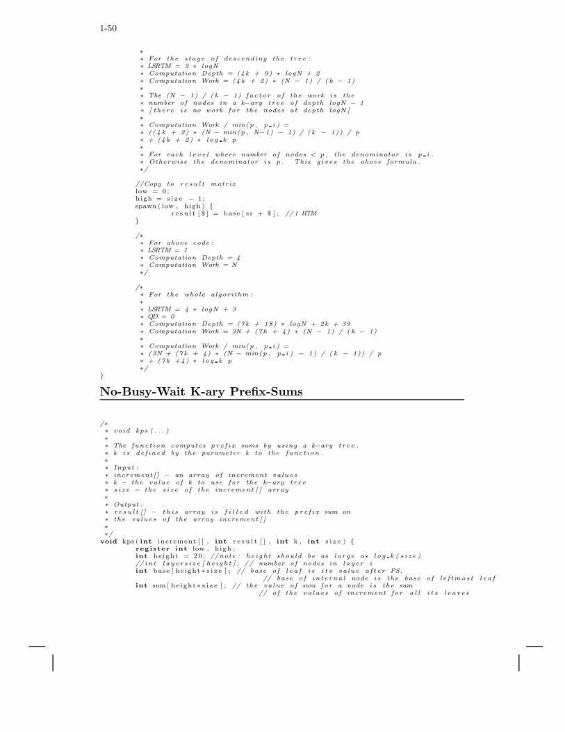
1-50
∗∗ For the stage of descending the t re e :∗ LSRTM = 2 ∗ logN∗ Computation Depth = (4k + 9) ∗ logN + 2∗ Computation Work = (4k + 2) ∗ (N − 1) / ( k − 1)∗∗ The (N − 1) / ( k − 1) fac tor of the work i s the∗ number of nodes in a k−ary t re e of depth logN − 1∗ [ there i s no work for the nodes at depth logN ]∗∗ Computation Work / min(p , p i ) =∗ ((4 k + 2) ∗ (N − min(p , N−1) − 1) / ( k − 1)) / p∗ + (4k + 2) ∗ l o g k p∗∗ For each l e v e l where number of nodes < p , the denominator i s p i .∗ Otherwise the denominator i s p . This g iv e s the above formula .∗/
//Copy to r e su l t matrixlow = 0;high = s i z e − 1;spawn ( low , high ) {
r e s u l t [ $ ] = base [ s r + $ ] ; //1 RTM}
/∗∗ For above code :∗ LSRTM = 1∗ Computation Depth = 4∗ Computation Work = N∗/
/∗∗ For the whole algorithm :∗∗ LSRTM = 4 ∗ logN + 3∗ QD = 0∗ Computation Depth = (7k + 18) ∗ logN + 2k + 39∗ Computation Work = 3N + (7k + 4) ∗ (N − 1) / ( k − 1)∗∗ Computation Work / min(p , p i ) =∗ (3N + (7k + 4) ∗ (N − min(p , p i ) − 1) / ( k − 1)) / p∗ + (7k +4) ∗ l o g k p∗/
}
No-Busy-Wait K-ary Prefix-Sums
/∗∗ void kps ( . . . )∗∗ The funct ion computes p r e f i x sums by using a k−ary t re e .∗ k i s de f ined by the parameter k to the funct ion .∗∗ Input :∗ increment [ ] − an array of increment va lues∗ k − the va lue of k to use for the k−ary t re e∗ s i z e − the s i z e of the increment [ ] array∗∗ Output :∗ r e s u l t [ ] − t h i s array i s f i l l e d with the p r e f i x sum on∗ the va lues of the array increment [ ]∗∗/
void kps ( int increment [ ] , int r e s u l t [ ] , int k , int s i z e ) {register int low , high ;int he ight = 20 ; //note : he igh t should be as l a rg e as l o g k ( s i z e )// in t l a y e r s i z e [ he igh t ] ; / / number of nodes in laye r iint base [ he ight ∗ s i z e ] ; // base of l e a f i s i t s va lue a f t e r PS,
// base of in t e rna l node i s the base of l e f tmos t l e a fint sum [ he ight∗ s i z e ] ; // the va lue of sum for a node i s the sum
// of the va lues of increment for a l l i t s l e ave s
Advancing PRAM Algorithms into Parallel Programs 1-51
int i s L ea f [ he ight ∗ s i z e ] ; // i f a l e a f : 1 ; i f not a l e a f : 0int passIndex [ he ight ∗ s i z e ] ; //array for passing index to c h i l d threads
int i t e r a t i o n = 0 ; // determines the current he igh t in the t re e
int temp ;int done ; //a loop contro l var iab l e
int l , // l e v e l where l eave s s t a r tsb , // index where l eave s would s t a r t i f s i z e i s a power of 2d , // s i z e − kˆ lo f f s e t , //how much to o f f s e t due to s i z e not being power of 2sr , // sb + o f f s e tover , //number of l e ave s at l e v e l lunder , //number of l e ave s at l e v e l l + 1sbp1 ; // index of one l e v e l h igher from sb
int f i l l ; //nodes to f i l l in with 0 to make a l l nodes have k ch i l d ren
int l e v e l , s t a r t i ndex , l a y e r s i z e ;
int i ;
/∗∗ With non−b l ock ing wr i t e s 0 RTM is required to i n i t i a l i z e∗ the funct ion parameters : k and s i z e∗ 0 RTM is required to i n i t i a l i z e l o c a l v a r i a b l e s such as he igh t∗/
//Spec ia l case i f s i z e == 1i f ( s i z e == 1) { // the check has 0 RTM because s i z e i s cached .
r e s u l t [ 0 ] = 0 ;return ;
}
/∗∗ 21 l i n e s of code above , means computation cost = 21 up to t h i s point .∗/
// c a l c u l a t e l oca t ion for l eave s in the complete representat ionl = l og ( s i z e ) / l og (k ) ;
sb = (pow(k , l ) − 1 ) / ( k − 1 ) ; // t h i s i s der ived from geometric s e r i e ssbp1 = (pow(k , l +1) − 1) / ( k − 1) ;
d = s i z e − pow(k , l ) ;o f f s e t = CEIL ( ( ( double ) d ) / ( k − 1 ) ) ;s r = sb + o f f s e t ;over = pow(k , l ) − o f f s e t ;under = s i z e − over ;
/∗∗ Computation cost = 8∗/
// p r in t f (” l = %d , sb = %d , d = %d , o f f s e t = %d , sr = %d , over = %d\n” , l , sb , d , o f f s e t , sr , over )
// Copy increment [ . . . ] to l eave s of sum [ . . . ]
low = 0;high = s i z e − 1;spawn ( low , high ) {
i f ( $ < under ) {sum [ $ + sbp1 ] = increment [ $ ] ; // 1 RTMi s L ea f [ $ + sbp1 ] = 1 ;
}else {
sum [ ( $ − under ) + sb + o f f s e t ] = increment [ $ ] ; //1 RTMi s L ea f [ ( $ − under ) + sb + o f f s e t ] = 1 ;
}} // 1 RTM jo in
/∗∗ For code above :∗
1-52
∗ LSRTM = 2∗ Computation Depth = 6∗ Computation Work = 3N∗/
// Make some 0 l eave s at l e v e l l +1 so a l l nodes have exac t l y// k ch i l d ren
f i l l = ( k − ( under % k )) % k ;for ( i = 0 ; i < f i l l ; i ++) {
sum [ sbp1 + under + i ] = 0 ;}
/∗∗ Computation Cost = 2k + 1∗/
//Climb t re e
low = sr ;high = sr + s i z e + f i l l − 1;spawn ( low , high ) {
int gate , count , a l i v e ;int index= $ ;a l i v e = 1;
while ( a l i v e ) {index = ( index − 1) / k ;
gate = 1;psm( gate , & gatekeeper [ index ] ) ; //1 RTM
i f ( gate == k − 1) {/∗∗ Using pre fe tching , the sum[X] elements∗ in the fo l l owing loop are read a l l at once∗ LSRTM = 1∗ ( pre fe t ch ing ) Computation Depth = k∗/
sum [ index ] = 0 ;for ( count = 0 ; count < k ; count++) {
sum [ index ] += sum [ k∗ index + count + 1 ] ;}
i f ( index == 0) {a l i v e = 0;
}
/∗∗ Computation Depth = 2k + 3;∗/
}else {
a l i v e = 0;}
}} // 1 RTM jo in
/∗∗ For code above :∗∗ LSRTM = 2 ∗ logN + 1∗ QD = k ∗ logN∗ Computation Depth = (8 + 2k ) ∗ ( logN + 1) + 6∗ Computation Work = (8 + 2k ) ∗ (N − 1) / ( k − 1) + 8N∗∗ The (N − 1) / ( k − 1) fac tor of the work comes∗ from counting the t o t a l nodes in a t re e with logN − 1∗ l e v e l s . Each of the l eave s at l e v e l logN only∗ executes the f i r s t 8 l i n e s ins ide the spawn b lock∗ ( tha t is , up to the check of the gatekeeper ) be fore∗ most die and only 1 thread per parent continues . This∗ g iv e s the 8N term .
Advancing PRAM Algorithms into Parallel Programs 1-53
∗∗ Computation Work / min(p , p i ) =∗ ((8 + 2 k )∗(N − min(p , N−1) − 1)/(k−1) + 8N) / p∗ + (8 + 2k ) ∗ l o g k p∗∗ For each l e v e l where number of nodes < p , the denominator i s p i .∗ Otherwise the denominator i s p . This g iv e s the above formula .∗/
base [ 0 ] = 0 ; // se t root base = 0
low = 0;high = 0;spawn ( low , high ) {
int count , tempbase ;int index = $ ;int newID ;
i f ( $ != 0 ) {index = passIndex [ $ ] ;
}
while ( i sL ea f [ index ] == 0) {tempbase = base [ index ] ;
/∗∗ The k − 1 c a l l s to sspawn can be executed with∗ a s i ng l e kspawn ins t ruc t ion .∗ The elements sum[X] are read a l l at once using∗ pre fe t ch ing .∗∗ LSRTM = 2∗ ( kspawn and pre fe t ch ing ) Computation Depth = k +1∗/
for ( count = 0 ; count < k ; count++) {base [ k∗ index + count + 1] = tempbase ;tempbase += sum [ k∗ index + count + 1 ] ;
i f ( count != 0) {sspawn (newID) {
passIndex [ newID ] = k∗ index + count + 1;}
}}
index = k∗ index + 1;
/∗∗ Computation Depth = 6k + 1∗/
}} //1 RTM jo in
/∗∗ For code above :∗∗ LSRTM = 2 ∗ logN + 1∗ Computation Depth = (3 + 6k ) ∗ logN + 9∗ Computation Work = (3 + 6k ) ∗ (N − 1) / ( k − 1) + 6N + 6∗∗ The (N − 1) / ( k − 1) fac tor of the work comes∗ from counting the t o t a l nodes in a t re e with logN − 1∗ l e v e l s . Each of the l eave s at l e v e l logN only∗ executes the f i r s t 6 l i n e s ins ide the spawn b lock∗ ( up to the check of isLeaf ) be fore dying . This∗ g iv e s the 6N term .∗∗ Computation Work / min(p , p i ) =∗ ((3 + 6 k )∗(N − min(p , N−1) − 1) / (k−1) + 6N + 6)/p∗ + (3 + 6k ) ∗ l o g k p∗/
//Copy to r e su l t matrix
1-54
low = 0;high = s i z e − 1;spawn ( low , high ) {
r e s u l t [ $ ] = base [ s r + $ ] ; //1 RTM} //1 RTM jo in
/∗∗ LSRTM = 2∗ Computation Depth = 4∗ Computation Work = N∗/
/∗∗ For the whole algorithm :∗∗ LSRTM = 4 ∗ logN + 6∗ QD = k ∗ logN∗ Computation Depth = (11 + 8k ) ∗ logN + 2k + 55∗ Computation Work = (11 + 8k ) ∗ (N − 1) / ( k − 1) + 18N + 6∗∗ Computation Work / min(p , p i ) =∗ ((11 + 8k )∗(N − min(p , N−1) − 1) / (k−1) + 18N + 6) / p∗ + (11 + 8k )∗ l o g k p∗/
}
Serial Summation
/∗∗ void sum ( . . . )∗ Function computes a sum∗∗ Input :∗ increment [ ] − an array of increment va lues∗ k − the va lue of k to use for the k−ary t re e∗ s i z e − the s i z e of the increment [ ] array∗∗ Output :∗ sum∗∗/
void sum( int increment [ ] , int ∗ sum , int k , int s i z e ) {int i ;∗sum = 0;
for ( i = 0 ; i < s i z e ; i ++) {∗sum += increment [ i ] ;
}
/∗∗ LSRTM = 1∗ At f i r s t , 1 RTM is needed to read increment . However , l a t e r reads∗ to increment are accomplished with pre fe t ch .∗∗ QD = 0∗ Computation = 2N∗/
}
Serial Prefix-Sums
/∗∗ void kps ( . . . )∗∗ The funct ion computes p r e f i x sums s e r i a l l y .∗∗ Input :∗ increment [ ] − an array of increment va lues∗ k − the va lue of k to use for the k−ary t re e ( not used )
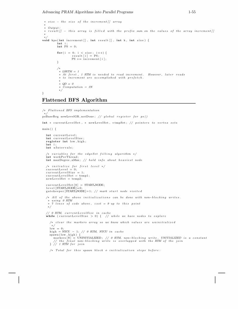
Advancing PRAM Algorithms into Parallel Programs 1-55
∗ s i z e − the s i z e of the increment [ ] array∗∗ Output :∗ r e s u l t [ ] − t h i s array i s f i l l e d with the p r e f i x sum on the va lues of the array increment [ ]∗∗/
void kps ( int increment [ ] , int r e s u l t [ ] , int k , int s i z e ) {int i ;int PS = 0;
for ( i = 0 ; i < s i z e ; i ++) {r e s u l t [ i ] = PS ;PS += increment [ i ] ;
}
/∗∗ LSRTM = 1∗ At f i r s t , 1 RTM is needed to read increment . However , l a t e r reads∗ to increment are accomplished with pre fe t ch .∗∗ QD = 0∗ Computation = 3N∗/
}
Flattened BFS Algorithm
/∗ Flat tened BFS implementation∗/
psBaseReg newLevelGR , notDone ; // g l ob a l r e g i s t e r for ps ()
int ∗ currentLeve lSe t , ∗ newLevelSet , ∗ tmpSet ; // pointers to ve r t e x s e t s
main ( ) {
int cu r r en tLeve l ;int cu r r en tLeve lS i z e ;register int low , high ;int i ;int n In t e r v a l s ;
/∗ v a r i a b l e s for the edgeSet f i l l i n g algorithm ∗/int workPerThread ;int maxDegree , nMax ; // hold in fo about heav ie s t node
/∗ i n i t i a l i z e for f i r s t l e v e l ∗/cu r r en tLeve l = 0;cu r r en tLeve lS i z e = 1;cu r r en tLeve lSe t = temp1 ;newLevelSet = temp2 ;
cu r r en tLeve lSe t [ 0 ] = START NODE;l e v e l [START NODE]=0;gatekeeper [START NODE]=1 ; // mark s t a r t node v i s i t e d
/∗ Al l o f the above i n i t i a l i z a t i o n s can be done with non−b l ock ing wr i t e s .∗ using 0 RTM∗ 7 l i n e s of code above , cost = 9 up to t h i s point∗/
// 0 RTM, currentLeve lSize in cachewhile ( cu r r en tLeve lS i z e > 0) { // whi le we have nodes to exp lore
/∗ c l ear the markers array so we know which va lues are u n i n i t i a l i z e d∗/
low = 0;high = NTCU − 1 ; // 0 RTM, NTCU in cachespawn ( low , high ) {
markers [ $ ] = UNINITIALIZED ; // 0 RTM, non−b l ock ing write . UNITIALIZED i s a constant// the f i n a l non−b l ock ing write i s overlapped with the RTM of the jo in
} // 1 RTM for jo in
/∗ Total for t h i s spawn b lock + i n i t i a l i z a t i o n s t eps be fore :
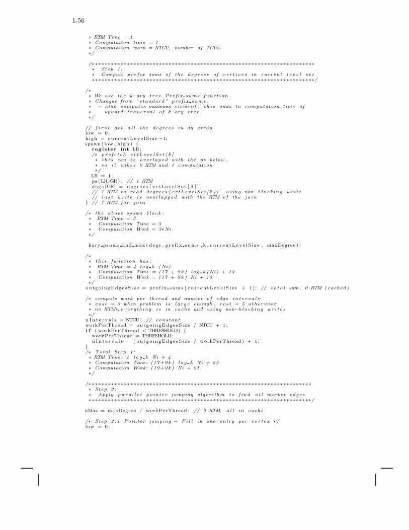
1-56
∗ RTM Time = 1∗ Computation time = 1∗ Computation work = NTCU, number of TCUs.∗/
/∗∗∗∗∗∗∗∗∗∗∗∗∗∗∗∗∗∗∗∗∗∗∗∗∗∗∗∗∗∗∗∗∗∗∗∗∗∗∗∗∗∗∗∗∗∗∗∗∗∗∗∗∗∗∗∗∗∗∗∗∗∗∗∗∗∗∗∗∗∗∗ Step 1 :∗ Compute pr e f i x sums of the degrees of v e r t i c e s in current l e v e l s e t∗∗∗∗∗∗∗∗∗∗∗∗∗∗∗∗∗∗∗∗∗∗∗∗∗∗∗∗∗∗∗∗∗∗∗∗∗∗∗∗∗∗∗∗∗∗∗∗∗∗∗∗∗∗∗∗∗∗∗∗∗∗∗∗∗∗∗∗∗∗/
/∗∗ We use the k−ary t re e Prefix sums funct ion .∗ Changes from ” standard ” pre f ix sums :∗ − a l so computes maximum element . t h i s adds to computation time of∗ upward t r a v e r s a l o f k−ary t re e∗/
// f i r s t ge t a l l the degrees in an arraylow = 0;high = cu r r en tLeve lS i ze −1;spawn ( low , high ) {
register int LR;/∗ pre fe t ch c r tLeve lSe t [ $ ]∗ t h i s can be over laped with the ps below ,∗ so i t takes 0 RTM and 1 computation∗/
LR = 1;ps (LR,GR) ; // 1 RTMdegs [GR] = degree s [ c r tLeve lS e t [ $ ] ] ;// 1 RTM to read degrees [ c r tLeve lSe t [ $ ] ] . using non−b l ock ing write// l a s t wri te i s overlapped with the RTM of the jo in
} // 1 RTM for jo in
/∗ the above spawn b lock :∗ RTM Time = 3∗ Computation Time = 3∗ Computation Work = 3∗Ni∗/
kary psums and max ( degs , pre f ix sums , k , cu r r en tLeve lS i ze , maxDegree ) ;
/∗∗ t h i s funct ion has :∗ RTM Time = 4 lo g k (Ni)∗ Computation Time = (17 + 9k ) l o g k (Ni) + 13∗ Computation Work = (17 + 9k ) Ni + 13∗/
outgo ingEdgesS ize = pre f i x sums [ cu r r en tLeve lS i z e + 1 ] ; // t o t a l sum. 0 RTM ( cached )
/∗ compute work per thread and number of edge in t e r va l s∗ cost = 3 when problem i s l a rg e enough , cost = 5 otherwise∗ no RTMs, everyth ing i s in cache and using non−b l ock ing wr i t e s∗/
n In t e r v a l s = NTCU; // constantworkPerThread = outgo ingEdgesS ize / NTCU + 1;i f ( workPerThread < THRESHOLD) {
workPerThread = THRESHOLD;n I n t e r v a l s = ( outgo ingEdgesS ize / workPerThread ) + 1 ;
}/∗ Total Step 1 :∗ RTM Time : 4 lo g k Ni + 4∗ Computation Time: (17+9k ) l o g k Ni + 23∗ Computation Work: (19+9k ) Ni + 21∗/
/∗∗∗∗∗∗∗∗∗∗∗∗∗∗∗∗∗∗∗∗∗∗∗∗∗∗∗∗∗∗∗∗∗∗∗∗∗∗∗∗∗∗∗∗∗∗∗∗∗∗∗∗∗∗∗∗∗∗∗∗∗∗∗∗∗∗∗∗∗∗∗ Step 2 :∗ Apply p a r a l l e l pointer jumping algorithm to f ind a l l marker edges∗∗∗∗∗∗∗∗∗∗∗∗∗∗∗∗∗∗∗∗∗∗∗∗∗∗∗∗∗∗∗∗∗∗∗∗∗∗∗∗∗∗∗∗∗∗∗∗∗∗∗∗∗∗∗∗∗∗∗∗∗∗∗∗∗∗∗∗∗∗/
nMax = maxDegree / workPerThread ; // 0 RTM, a l l in cache
/∗ Step 2 . 1 Pointer jumping − F i l l in one entry per ve r t e x ∗/low = 0;
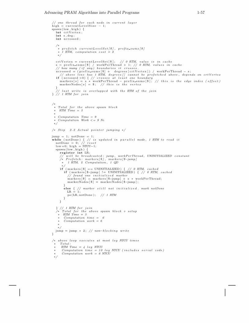
Advancing PRAM Algorithms into Parallel Programs 1-57
// one thread for each node in current l aye rhigh = cur r en tLeve lS i z e − 1;spawn ( low , high ) {
int c r tVertex ;int s , deg ;int ncrossed ;
/∗∗ pre fe t ch currentLeve lSe t [ $ ] , pre f ix sums [ $ ]∗ 1 RTM, computation cost = 2∗/
c r tVertex = cu r r en tLeve lSe t [ $ ] ; // 0 RTM, va lue i s in caches = pre f i x sums [ $ ] / workPerThread + 1 ; // 0 RTM, va lues in cache// how many ( i f any ) boundaries i t crosses .ncrossed = ( p r e f i x sums [ $ ] + degree s [ c r tVertex ] ) / workPerThread − s ;
// above l i n e has 1 RTM, degrees [ ] cannot be pre fe tched above , depends on crtVertexi f ( ncrossed >0) { // crosses at l e a s t one boundary
markers [ s ] = s ∗ workPerThread − pre f i x sums [ $ ] ; // t h i s i s the edge index ( o f f s e t )markerNodes [ s ] = $ ; // t h i s i s the ve r t e x
}// l a s t wri te i s overlapped with the RTM of the jo in
} // 1 RTM for jo in
/∗∗ Total for the above spawn b lock∗ RTM Time = 3∗∗ Computation Time = 9∗ Computation Work <= 9 Ni∗/
/∗ Step 2 .2 Actual pointer jumping ∗/
jump = 1 ; notDone = 1;while ( notDone ) { // i s updated in pa r a l l e l mode , 1 RTM to read i t
notDone = 0 ; // re se tlow =0; high = NTCU−1;spawn ( low , high ) {
register int LR;// w i l l be broadcasted : jump , workPerThread , UNINITIALIZED constant/∗ Prefe tch : markers [ $ ] , markers [ $−jump ]∗ 1 RTM, 2 Computation , 1 QD∗/
i f ( markers [ $ ] == UNINITIALIZED ) { // 0 RTM, cachedi f ( markers [ $−jump ] != UNINITIALIZED ) { // 0 RTM, cached
// found one i n i t i a l i z e d markermarkers [ $ ] = markers [ $−jump ] + s ∗ workPerThread ;markerNodes [ $ ] = markerNodes [ $−jump ] ;
}else { // marker s t i l l not i n i t i a l i z e d . mark notDone
LR = 1;ps (LR, notDone ) ; // 1 RTM
}}
} // 1 RTM for jo in/∗ Total for the above spawn b lock + setup∗ RTM Time = 3∗ Computation time = 6∗ Computation work = 6∗∗/
jump = jump ∗ 2 ; // non−b l ock ing write}
/∗ above loop executes at most l og NTCU times∗ Total :∗ RTM Time = 4 log NTCU∗ Computation time = 10 log NTCU ( inc lude s s e r i a l code )∗ Computation work = 6 NTCU∗/
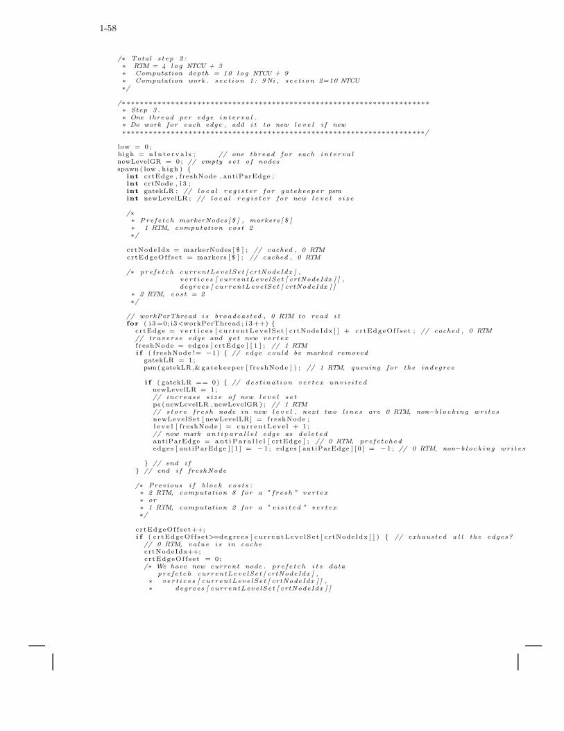
1-58
/∗ Total s tep 2 :∗ RTM = 4 log NTCU + 3∗ Computation depth = 10 log NTCU + 9∗ Computation work . se c t ion 1 : 9Ni , se c t ion 2=10 NTCU∗/
/∗∗∗∗∗∗∗∗∗∗∗∗∗∗∗∗∗∗∗∗∗∗∗∗∗∗∗∗∗∗∗∗∗∗∗∗∗∗∗∗∗∗∗∗∗∗∗∗∗∗∗∗∗∗∗∗∗∗∗∗∗∗∗∗∗∗∗∗∗∗∗ Step 3 .∗ One thread per edge in t e r v a l .∗ Do work for each edge , add i t to new l e v e l i f new∗∗∗∗∗∗∗∗∗∗∗∗∗∗∗∗∗∗∗∗∗∗∗∗∗∗∗∗∗∗∗∗∗∗∗∗∗∗∗∗∗∗∗∗∗∗∗∗∗∗∗∗∗∗∗∗∗∗∗∗∗∗∗∗∗∗∗∗∗/
low = 0;high = n In t e r v a l s ; // one thread for each i n t e r va lnewLevelGR = 0 ; // empty se t o f nodesspawn ( low , high ) {
int crtEdge , freshNode , antiParEdge ;int crtNode , i 3 ;int gatekLR ; // l o c a l r e g i s t e r for gatekeeper psmint newLevelLR ; // l o c a l r e g i s t e r for new l e v e l s i z e
/∗∗ Prefe tch markerNodes [ $ ] , markers [ $ ]∗ 1 RTM, computation cost 2∗/
crtNodeIdx = markerNodes [ $ ] ; // cached , 0 RTMc r tEdgeOf f se t = markers [ $ ] ; // cached , 0 RTM
/∗ pre fe t ch currentLeve lSe t [ crtNodeIdx ] ,v e r t i c e s [ currentLeve lSe t [ crtNodeIdx ] ] ,degrees [ currentLeve lSe t [ crtNodeIdx ] ]
∗ 2 RTM, cost = 2∗/
// workPerThread i s broadcasted , 0 RTM to read i tfor ( i 3 =0; i3<workPerThread ; i 3++) {
crtEdge = ve r t i c e s [ c u r r en tLeve lSe t [ crtNodeIdx ] ] + crtEdgeOf f se t ; // cached , 0 RTM// trave r se edge and get new ver t e xf reshNode = edges [ crtEdge ] [ 1 ] ; // 1 RTMi f ( f reshNode != −1) { // edge could be marked removed
gatekLR = 1;psm(gatekLR,&gatekeeper [ f reshNode ] ) ; // 1 RTM, queuing for the indegree
i f ( gatekLR == 0) { // de s t ina t ion ve r t e x unv i s i t ednewLevelLR = 1;// increase s i z e of new l e v e l s e tps ( newLevelLR , newLevelGR ) ; // 1 RTM// s tore f r e sh node in new l e v e l . next two l i n e s are 0 RTM, non−b l ock ing wr i t e snewLevelSet [ newLevelLR] = freshNode ;l e v e l [ f reshNode ] = cu r r en tLeve l + 1;// now mark an t i p a r a l l e l edge as de l e t edantiParEdge = an t i P a r a l l e l [ crtEdge ] ; // 0 RTM, pre fe tchededges [ antiParEdge ] [ 1 ] = − 1 ; edges [ antiParEdge ] [ 0 ] = − 1 ; // 0 RTM, non−b l ock ing wr i t e s
} // end i f} // end i f freshNode
/∗ Previous i f b lock cos t s :∗ 2 RTM, computation 8 for a ” f re sh ” ve r t e x∗ or∗ 1 RTM, computation 2 for a ” v i s i t e d ” ve r t e x∗/
c r tEdgeOf f se t++;i f ( c r tEdgeOf f se t>=degree s [ c u r r en tLeve lS e t [ crtNodeIdx ] ] ) { // exhausted a l l the edges?
// 0 RTM, va lue i s in cachecrtNodeIdx++;crtEdgeOf f se t = 0;/∗ We have new current node . pre fe t ch i t s data
pre fe t ch currentLeve lSe t [ crtNodeIdx ] ,∗ ve r t i c e s [ currentLeve lSe t [ crtNodeIdx ] ] ,∗ degrees [ currentLeve lSe t [ crtNodeIdx ] ]
Advancing PRAM Algorithms into Parallel Programs 1-59
∗ 2 RTM, cost = 2∗/
}
/∗ This i f and ins t ruc t ion be fore i t cost :∗ 2 RTM, 6 computation for each new marker edge in in t e r va l∗ or∗ 2 computation for a l l other edges∗/
i f ( crtNodeIdx>= cur r en tLeve lSe t )break ;
// t h i s i f i s 0 RTM, 1 computation .
} // end for
/∗ Previous loop i s executed C = Ei/p times .∗ We assume Ni nodes are ” f re sh ” , worst case ana lys i s∗ Total over a l l i t e r a t i on s . AA i s the number of marker edges in in t e r v a l .∗ WITHOUT PREFETCHING:∗ RTM: 3∗C + 2 AA∗ Computation : 11∗C + 4 AA∗/
// l a s t wri te i s overlapped with the RTM of the jo in} // 1 RTM for jo in
/∗∗ Total for above spawn b lock + i n i t i a l i z a t i o n : (C=Ei/p , AA = N/p = # marker edges )∗ WITHOUT PREFETCHING for mu l t ip l e edges : RTM Time = 3∗C + 3 + 2 AA∗ WITH PREFETCHING for mu l t ip l e edges : RTM Time = 3 + 3 + 2∗ Computation Time = 8 + 7∗C + 16 AA∗ Computation Work = 8p + 7E + 16N∗/
// move to next l aye rcu r r en tLeve l++;cu r r en tLeve lS i z e = newLevelGR ; // from the pre f i x−sums// ” swap” currentLeve lSe t with newLevelSettmpSet = newLevelSet ;newLevelSet = cu r r en tLeve lSe t ;c u r r en tLeve lS e t = tmpSet ;
/∗ a l l these above s t eps : 0 RTM, 5 computation ∗/
} // end whi le/∗∗ Total for one BFS l e v e l ( one i t e r a t i on of above whi le loop ) :∗ W/O PRE: RTM Time = 4 lo g k Ni + 4 |Ei |/ p + 11 + LSRTM of PSUMS∗ W PRE : RTM Time = 4 lo g k Ni + 4 + 11 + LSRTM of PSUMS∗ Computation Time =∗ Comp Work =∗/
}
Single-Spawn BFS Algorithm
/∗ BFS implementation using s ing l e−spawn operation∗ for nest ing∗/
psBaseReg newLevelGR ; // g l o ba l r e g i s t e r for new l e v e l s e t
int ∗ currentLeve lSe t , ∗ newLevelSet , ∗ tmpSet ; // pointers to l e v e l s e t s
main ( ) {
int cu r r en tLeve l ;int cu r r en tLeve lS i z e ;int low , high ;int i ;
c u r r en tLeve l = 0;cu r r en tLeve lS i z e = 1;
1-60
cu r r en tLeve lSe t = temp1 ;newLevelSet = temp2 ;
cu r r en tLeve lSe t [ 0 ] = START NODE; // s tore the ve r t e x# th i s thread w i l l handle
/∗∗ 0 RTMs, 5 computation∗/
while ( cu r r en tLeve lS i z e > 0) { // whi le we have nodes to exp lorenewLevelGR = 0;low = 0;high = cu r r en tLeve lS i z e − 1 ; // one thread for each node in current l aye r
spawn ( low , high ) {int gatekLR , newLevelLR , newTID ;int freshNode , antiParEdge ;
/∗∗ Al l threads need to read t he i r i n i t i a l i z a t i o n data∗ nForks [ $ ] and currentEdge [ $ ]∗/
i f ( $ < cu r r en tLeve lS i z e ) { // 0 RTM/∗∗ ” Orig ina l ” threads read i t e x p l i c i t l y from the graph∗/
// only s t a r t degree−1 new threads , current thread w i l l handle one edgenForks [ $ ] = degree s [ c u r r en tLeve lS e t [ $ ] ] − 1 ; // 2 RTM// th i s thread w i l l handle f i r s t outgoing edgecurrentEdge [ $ ] = v e r t i c e s [ c u r r en tLeve lS e t [ $ ] ] ; // 1 RTM
}else {
/∗∗ Single−spawned threads , need to ” wait ” un t i l i n i t va lues∗ from the parent are wri t ten∗/
while ( l o ck s [ $ ] ! = 1 ) ; // busy wait un t i l i t g e t s the s i gna l
} // end i f
/∗ The above i f b lock takes∗ 3 RTM, 3 computation for ” o r i g i na l ” threads∗ for c h i l d threads : 1 RTM for synchronizat ion . 2 computation∗/
while ( nForks [ $ ] > 0 ) { // 1 computation// t h i s i s executed for each c h i l d thread spawnedsspawn(newTID ) { // 1 RTM/∗∗ writ ing i n i t i a l i z a t i o n data for c h i l d threads .∗ ch i l d ren w i l l wait t i l l t h i s data i s commited∗/nForks [ newTID ] = ( nForks [ $ ]+1)/2 −1;nForks [ $ ] = nForks [ $ ] − nForks [ newTID]−1;currentEdge [ newTID ] = currentEdge [ $ ] + nForks [ $ ]+1;l o ck s [ newTID ] = 1 ; // GIVE THE GO SIGNAL!
/∗∗ 0 RTM∗ 4 computation∗/
}/∗ For each c h i l d thread :∗ 1 RTM∗ 5 computation∗/
} // done with fork ing
/∗∗ Prefe tch edges [ currentEdge [ $ ] ] [ 1 ] , an t iPa ra l l e l [ currentEdge [ $ ] ]∗ 1 RTM, 2 computation∗/
Advancing PRAM Algorithms into Parallel Programs 1-61
// l e t ’ s handle one edgef reshNode = edges [ currentEdge [ $ ] ] [ 1 ] ; // 0 RTM, va lue was pre fe tchedi f ( f reshNode != −1 ) { // i f edge hasn ’ t been de l e t ed
gatekLR = 1;// t e s t gatekeeperpsm(gatekLR,&gatekeeper [ f reshNode ] ) ; // 1 RTM. GQD queuing
i f ( gatekLR == 0) { // de s t ina t ion ve r t e x unv i s i t ed !newLevelLR = 1;// increase s i z e of new l e v e l s e tps ( newLevelLR , newLevelGR ) ; // 1 RTM// s tore f r e sh node in new l e v e lnewLevelSet [ newLevelLR] = freshNode ;l e v e l [ f reshNode ] = cu r r en tLeve l + 1;// now mark a n t i p a r a l l e l edge as de l e t edantiParEdge = an t iP a r a l l e l [ currentEdge [ $ ] ] ; // 0 RTM, va lue was pre fe tchededges [ antiParEdge ] [ 1 ] = −1 ;edges [ antiParEdge ] [ 0 ] = −1 ;
} // end i f} // end i f
/∗∗ Previous i f b lock cos t s :∗ 2 RTM, 10 computation for ” f re sh ” ve r t e x∗ 0 RTM, 2 computation for v i s i t e d ve r t e x
∗/
/∗∗ Final wri te i s b lock ing , but the RTM over laps the jo in .∗/
} // 1 RTM jo in
/∗ Computation for a c h i l d thread tha t s t a r t s one s i ng l e c h i l d : 1 9 ∗/
// move to next l aye rcu r r en tLeve l++;cu r r en tLeve lS i z e = newLevelGR ; // from the pre f i x−sums// ” swap” currentLeve lSe t with newLevelSettmpSet = newLevelSet ;newLevelSet = cu r r en tLeve lSe t ;c u r r en tLeve lS e t = tmpSet ;
/∗ the above 5 l i n e s of code : 0 RTM, 5 computation ∗/
} // end whi le}
k-Spawn BFS Algorithm
The only difference between the single-spawn BFS algorithm and the k-spawn is the whileloop that is starting children threads. We’re including only that section of the code here,the rest is identical with the code in the BFS Single-Spawn implementation.
while ( nForks [ $ ] > 0 ) { // 1 computation// t h i s i s executed for each c h i l d thread spawnedkspawn (newTID ) { // 1 RTM for kSpawn
// newTID i s the lowest o f the k TIDs a l l oca ted by k−spawn .// The other ones are newTID+1, newTID+2 , . . . , newTID+(k−1)
/∗∗ writ ing i n i t i a l i z a t i o n data for c h i l d threads .∗ ch i l d ren w i l l wait t i l l t h i s data i s commited∗/
s l i c e = nForks [ $ ] / k ;nForks [ $ ] = nForks [ $ ] − s l i c e ; // sub s t rac t a s l i c e for parent thread
for ( ch i l d =0; ch i ld <k ; c h i l d ++) {// i n i t i a l i z e nForks [ newTid + ch i l d ] and currentEdge [ newTid + ch i l d ]nForks [ newTID + ch i l d ] = max( s l i c e , nForks [ $ ] ) ; // for roundingcurrentEdge [ newTID ] = currentEdge [ $ ] + ch i l d ∗ s l i c e ;
1-62
nForks [ $ ] = nForks [ $ ] − nForks [ newTID + ch i l d ] ;l o c k s [ newTID + ch i l d ] = 1 ; // GIVE THE GO SIGNAL!
}/∗∗ loop i s executed k times .∗ Each i t e r r a t i on :∗ 0 RTM∗ 4 computation∗/
}/∗ For each k c h i l d threads :∗ 1 RTM∗ 2+4∗k computation∗/
} // done with fork ing


![Planarity Testing in Parallel - Duke Universityreif/paper/rama/planarity.pdfKarp & Ramachandran [KR90] for a discussion of parallel algorithms on various PRAM models.) More precisely,](https://static.fdocuments.in/doc/165x107/61020de460a8a04ed5618c54/planarity-testing-in-parallel-duke-university-reifpaperrama-karp-ramachandran.jpg)