General rights Copyright and moral rights for the publications made accessible in the public portal are retained by the authors and/or other copyright owners and it is a condition of accessing publications that users recognise and abide by the legal requirements associated with these rights.

Users may download and print one copy of any publication from the public portal for the purpose of private study or research.

You may not further distribute the material or use it for any profit-making activity or commercial gain

You may freely distribute the URL identifying the publication in the public portal If you believe that this document breaches copyright please contact us providing details, and we will remove access to the work immediately and investigate your claim.

Downloaded from orbit.dtu.dk on: Apr 08, 2022

Models and Methods for Free Material Optimization

Weldeyesus, Alemseged Gebrehiwot

Publication date:2014

Document VersionPublisher's PDF, also known as Version of record

Link back to DTU Orbit

Citation (APA):Weldeyesus, A. G. (2014). Models and Methods for Free Material Optimization. DTU Wind Energy. DTU WindEnergy PhD No. 0041(EN)

Models and Methods for Free MaterialOptimization

Alemseged Gebrehiwot Weldeyesus

Department of Wind EnergyTechnical University of Denmark (DTU)

Author: Alemseged Gebrehiwot WeldeyesusTitle: Models and Methods for Free Material Opti-mizationDivision: Department of Wind Energy

The thesis is submitted to the Danish Technical Uni-versity in partial fulfillment of the requirements for thePhD degree.

2014

Project Period;2010-2014

Degree:Phd

Supervisors:Mathias StolpeErik Lund

ISBN: 978-87-92896-89-6

Sponsorship:Danish Council for StrategicResearch Council through theDanish Center for CompositeStructures and Materials(DCCSM)

Technical University of Den-markDepartment of Wind EnergyFrederiksborgvej 399Building 1184000 RoskildeDenmarkTelephone: (+45)20683230Email: alwel@dtu.dkwww.vindenergi.dtu.dk

AbstractFree Material Optimization (FMO) is a powerful approach for structural opti-mization in which the design parametrization allows the entire elastic stiffnesstensor to vary freely at each point of the design domain. The only requirementimposed on the stiffness tensor lies on its mild necessary conditions for physicalattainability, in the context that, it has to be symmetric and positive semidefi-nite. FMO problems have been studied for the last two decades in many articlesthat led to the development of a wide range of models, methods, and theories.

As the design variables in FMO are the local material properties any resultsusing coarse finite element discretization are not essentially predictive. Besidesthe variables are the entries of matrices at each point of the design domain.Thus, we face large-scale problems that are modeled as nonlinear and mostly nonconvex semidefinite programming. These problems are more difficult to solve anddemand higher computational efforts than the standard optimization problems.The focus of today’s development of solution methods for FMO problems is basedon first-order methods that require a large number of iterations to obtain optimalsolutions. The scope of the formulations in most of the studies is indeed limitedto FMO models for two- and three-dimensional structures. To the best of ourknowledge, such models are not proposed for general laminated shell structureswhich nowadays have extensive industrial applications.

This thesis has two main goals. The first goal is to propose an efficient op-timization method for FMO that exploits the sparse structures arising from themany small matrix inequality constraints. It is developed by coupling second-order primal dual interior point solution techniques for the standard nonlinearoptimization problems and linear semidefinite programs. The method has suc-cessfully obtained solutions to large-scale classical FMO problems of simultaneousanalysis and design, nested and dual formulations. The second goal is to extendthe method and the FMO problem formulations to general laminated shell struc-tures.

The thesis additionally addresses FMO problem formulations with stress con-straints. These problems are highly nonlinear and lead to the so-called singularityphenomenon. The method described in the thesis has successfully solved theseproblems. In the numerical experiments the stress constraints have been satisfiedwith high feasibility tolerances.

The thesis further includes some preliminary numerical progresses on solvingFMO problems using iterative solvers.

i

Resumé (In Danish)Fri Materiale Optimering (FMO) er en kraftfuld metode inden for strukturel op-timering, hvori parametriseringen af designet tillader den fulde elastiske stivhed-stensor at variere frit i ethvert punkt i designområdet. Det eneste krav til stivhed-stensoren ligger i de svage betingelser om fysisk opnåelighed, hvilket vil sige, atden skal være symmetrisk og positiv semi-definit. Indenfor de seneste to årtierer problemer inden for FMO blevet studeret i en lang række artikler, hvilket haraffødt en bred vifte af modeller, metoder og teorier.

Da design-parametrene i FMO er lokale egenskaber ved materialet, er ethvertdesignresultat baseret på en grov diskretisering med finite element metoden ikkeprædiktivt. Hertil kommer det faktum at variablene er matrix-elementer i ethvertpunkt i designdomænet. Vi har altså at gøre med stor-skala-problemer, som skalmodelleres vha. ikke-lineær og primært ikke-konveks semi-definit programmer-ing. Sådanne problemer er sværere at løse og mere beregningstunge end al-mindelige optimeringsproblemer. Udviklingen af metoder til problemer indenforFMO fokuserer i dag på førsteordens metoder, som kræver et stort antal itera-tioner for at opnå optimale løsninger. Rammerne for formuleringerne i de flestestudier er begrænset til 2- og 3-dimensionale strukturer. Sådanne modeller er- efter vores bedste overbevisning - ikke fremsat for generelle laminerede skal-strukturer, som i dag finder bred anvendelse i industrien.

Denne afhandling har to hovedformål. Det første formål er fremsætte en ef-fektiv optimeringsmetode inden for FMO, som udnytter den sparse struktur, derkommer fra de mange små matrix-uligheder som bibetingelser. Den er udvikletved at koble andenordens primal-dual interior point løsningsteknikker for almin-delige ikke-lineære optimeringsproblemer med lineære semi-definite programmer.Metoden er med succes blevet anvendt til at løse klassiske problemer indenforFMO på stor skala med samtidig analyse og design, i både indlejret og dual for-mulering. Det andet mål er at udvide metoden og formuleringerne af problemerneinden for FMO til generelle laminerede skal-strukturer.

Afhandlingen behandler desuden problemformuleringer inden for FMO, somindeholder betingelser på stress. Disse problemer er stærkt ikke-lineære og giveranledning til såkaldte singularitetsfænomener. Metoden, som er beskrevet i denneafhandling, har med succes løst sådanne problemer. Stress-betingelserne er blevetopfyldt med en høj tolerance på gennemførligheden i de numeriske eksperimenter.

Afhandlingen indeholder desuden foreløbigt arbejde vedrørende løsning afproblemer inden for FMO ved brug af iterative løsere.

ii

PrefaceThis thesis was submitted in partial fulfillment of the requirements for obtainingthe PhD degree at the Technical University of Denmark. The work was doneat the Department of Mathematics from December 2010 to April 2011 and atthe Wind Turbine Structures section of the Department of Wind Energy fromMay 2011 to August 2014. The period includes about six months of paternityleave. The PhD project was funded by the Danish Council for Strategic Researchthrough the Danish Center for Composite Structures and Materials (DCCSM).Supervisor on the project was Senior Researcher Dr.Techn. Mathias Stolpe andco-supervisor was Professor Erik Lund.

First and foremost I would like to express my special gratitude and thanksto my supervisor for his guidance, support, and for always offering his timefor discussions. My special thanks extend to my co-supervisor for his fruitfuldiscussions on composites and valuable comments on my results. I am very muchgrateful to Dr. Stefanie Gaile for her discussions on Free Material Optimizationproblems and the development of finite element codes.

It was a pleasure for me to be part of the wonderful people in the Departmentof Mathematics and Department of Wind Energy.

A special thank to my friends and family. Thanks mom. Last but not theleast, I would like to thank my wife Helen and my daughter Mia for all the loveand encouragement.

Roskilde, August 2014

Alemseged Gebrehiwot Weldeyesus

iii

Contents

I Background v

1 Introduction 1

2 Free Material Optimization 42.1 The underlying FMO problem formulations . . . . . . . . . . . . . 5

2.1.1 FMO for solid structures . . . . . . . . . . . . . . . . . . . 62.1.2 FMO for laminated plates and shells . . . . . . . . . . . . . 7

2.2 The primal-dual interior point method . . . . . . . . . . . . . . . . 11

3 Summary of the articles 12

4 Conclusions, contributions and future research areas 144.1 Conclusions and contributions . . . . . . . . . . . . . . . . . . . . . 144.2 Future research areas . . . . . . . . . . . . . . . . . . . . . . . . . . 15

II Articles 21

5 A Primal-Dual Interior Point Method for Large-Scale Free Ma-terial Optimization 22

6 Free Material Optimization for Laminated Plates and Shells 56

7 Models and methods for Free Material Optimization with localstress constraints 84

8 On solving Free Material Optimization problems using iterativemethods 114

iv

Part I

Background

v

Chapter 1

Introduction

There has been remarkable advancement in manufacturing techniques for com-posite structures in the recent decades. This has given a rise to the application ofstructural optimization in industries to produce a wide range of light weight struc-tures. Structural optimization is a discipline that deals with the improvementof the mechanical performance of load carrying structures. The most commonmeasures of structural performance are weight, stiffness, stresses, strains, criticalloads, displacements and geometry. The optimization problems can thus be for-mulated by taking one or more of these measures as an objective function andsome of the other measures as constraints. The choice of geometric features orthe size of the set of admissible materials lead to several forms of structural opti-mization. Topology optimization introduced in [33] for truss structures and in [5]for continuum structures is one of the general forms that concerns with obtaining(almost) 0-1 optimal distribution of materials in a given design space. It is aclass of structural optimization that has been extensively studied with extremelydiversified approaches of problem formulations and solution methods, see e.g.[6]. Discrete Material Optimization introduced in [34], [35], and [25] concernswith optimal design of laminated composite structures by determining the bestdiscrete material selection, stacking sequence, and thickness distribution. Thereare further studies treating problem formulations involving more design criteriasuch as eigenfrequencies in [26] and buckling loads in [24]. These articles useparametrization based on weighting functions for optimal material selection. In[10] new approach for parameterization based on shape functions is proposed.The set of admissible materials can be extended further avoiding any restrictionto pre-existing materials and searching for more general material properties. Thisleads to the most general form the so-called Free Material Optimization (FMO)which deals with determining the optimal material distribution and the optimal

1

local material properties of structures through the stiffness tensors.The development of an efficient solution techniques and new FMO models are

the main goals of the thesis. One of the main motivations concerns the natureand size of FMO problems. As the design variables in FMO are the stiffnesstensors at each point of the design domain it is important to work with relativelyfine finite element discretizations to obtain essentially predictive solutions. Thenumber of independent variables in each stiffness tensor is 6 for two-dimensional,21 for three-dimensional, and 9 for problems on (thick) shells. Hence, we of-ten face large-scale problems. Moreover, the problems are modeled as nonlinear(and non convex) SemiDefinite Programming (SDP) for which studies on the-ories and numerical methods are much more recent than linear SDP problemsand standard optimization problems. Solving large-scale problems of this classlead to high computational complexity that often demands specialized solutiontechniques. For this reason researches on FMO problems are mostly accompaniedwith solution techniques, see Chapter 2. The focus of most of today’s develop-ment of optimization methods for FMO problems is based on first-order methodsthat often leads to large number of iterations. Second-order methods are consid-ered computationally too expensive. The thesis proposes a second-order interiorpoint method that efficiently utilizes the structure that each of the many matrixinequalities in FMO is small giving sparse structures in the optimization process.It is developed by coupling existing primal-dual interior point method for stan-dards nonlinear programming, see e.g. [13], [14], and [7], and the techniques forlinear SDP, see e.g. [29]. The method is also inspired by the recent developmentsin interior point methods for general nonlinear SDP problems, see e.g. [42] and[41]. Another motivation is the scope of the available FMO models. Most ofthese deal with FMO problems for two- and three-dimensional structures. Asfar as to our knowledge, no FMO models have been proposed in the literaturefor general laminated structures which are nowadays used in many engineeringapplications. The thesis proposes new FMO models for laminated plates andshells by extending the formulations in [15].

The thesis is organized in two parts. In Part I the introduction to the courseof the study is addressed. In Chapter 2 the review of the researches on FMO, theunderlying FMO problem formulations for solids and laminated structures, andthe overview of the method proposed in the thesis are described. The summaryof the papers included in the thesis is presented in Chapter 3. The conclusions,contributions and proposed research areas of the thesis are presented in Chapter4. Part II includes 4 papers listed below.

Chapter 5 Weldeyesus, A.G., Stolpe, M.: A primal-dual interior point methodfor largescale free material optimization. Computational Optimiza-tion and Applications (2014). DOI 10.1007/s10589-014-9720-6

2

Chapter 6 Weldeyesus, A.G., Stolpe, M.: Free Material Optimization for Lami-nated Plates and Shells. Journal of Structural and MultidisciplinaryOptimization. Accepted in 2014 and in print.

Chapter 7 Weldeyesus, A.G.: Models and methods for Free Material Optimiza-tion with local stress constraints. Submitted to Journal of Structuraland Multidisciplinary Optimization in 2014. In review.

Chapter 8 Stolpe, M., Weldeyesus, A.G.: On solving Free Material Optimiza-tion problems using iterative methods. Department of Wind Energy,Technical University of Denmark, 2014. To be submitted.

3

Chapter 2

Free Material Optimization

The design parametrization in Free Material Optimization (FMO) varies the en-tire stiffness tensor freely at each point of the design domain. We impose onlycertain requirements on the material tensor as necessary conditions on physi-cal attainability. The stiffness tensors are forced to be symmetric and positivesemidefinite. FMO obtains conceptual optimal structures characterized by opti-mal material distribution and optimal material properties which can be regardedas ultimately best structures among other possible elastic continua [43]. FMOthus can be used to generate benchmark solutions for other models and besidesto propose novel ideas for new design situations. For instance, in [23] we can seeconceptual optimal design of ribs in the leading edge of Airbus A380 that led tosubstantial weight reduction.

The basic FMO problem formulations of minimizing compliance dates back tothe 1990s in [3], [4], and [32]. Recent FMO models more are advanced than theseformulations taking in to account several engineering constraints. FMO modelsaiming at limiting high stresses, which often cause failures in engineering struc-tures, are introduced and solved in [23], [22], and [21] for two-dimensional andin [16] for three-dimensional structures. The models are further extended to ad-dress certain prescribed deformation behaviors through displacement constraintsin [23] and [16]. We find FMO formulations with eigenfrequency constraints in[38] that take in to account dynamic processes. In analogy to these multidisci-plinary problem formulations, FMO models for shells and plates are proposed in[15] to get designs more suited for thin-walled structures.

Considering the size and structure of FMO problems it is crucial that spe-cial purpose methods are preferred to general methods. For similar argumentsand details, see e.g. [37]. Small size FMO problems of slightly different ma-trix inequality constraints than recent FMO problems were solved in [32] with

4

an interior point method. A method based on penalty/barrier multipliers calledPBM is developed and is used to solve FMO problems in [43]. A computer codePENNON based an augmented Lagrangian function method developed in [20] tosolve convex nonlinear and SemiDefinite Programming (SDP) and further stud-ied in [36] is used to solve multidisciplinary FMO problems in several articles,e.g. stress constrained problems in [21] and displacement and stress constrainedproblems in [23]. A method based on a sequential convex programming conceptin which the subproblems are convex and separable SDPs is developed in [40, 39]and have been used to solve FMO problems in, e.g [16].

Theoretical treatments of FMO problems have been analyzed in several arti-cles. The existence of optimal solution to FMO problems is shown in the earlystudies [2] and [43] and latter in [27] based on saddle-point point theory and in[27] based on duality theory. These theories are not applicable when the engi-neering constraints mentioned above are included in the problem formulations.In [16] a generic FMO problem intended to take in to account displacement andstress constraints is formulated for which existence of solution is shown using amathematical tool described as H-convergence. The article indeed shows the con-vergence of the solution of the finite element discretized problems to the solutionof the original problem.

There are studies focusing on the post processing of FMO results to approxi-mate the conceptual designs with real materials suited for manufacturing process.In [18] the realization of FMO results by composite materials has been described.There are tools developed in [9] and [8] offering various possibilities and tech-niques of FMO data realization and visualization.

2.1 The underlying FMO problem formulationsIn this section we present the underlining minimum compliance (maximum stiff-ness) FMO problem formulation for two- and three-dimensional solids and lam-inated plates and shells. In both cases we start with the discrete version of theproblem formulation. The problem formulations and finite element discretiza-tion for solids closely follow, e.g. [40] and [23]. For the problems on laminatedstructures we refer the reader to [11] for details on the shell kinematics and toChapter 7 for the FMO problem formulations in function spaces and the finiteelement discretization.

In the optimization problems we consider the material tensor is in generalanisotropic, the loads are static and linear elasticity is assumed. From physicalattainability point of view the stiffness tensor has to be symmetric and positivesemidefinite. We follow the approach in most articles for choosing the trace ofthe stiffness tensor to measure material stiffnesses. We locally bound from aboveby ρ to avoid arbitrarily stiff materials and from below by ρ to limit softness. The

5

bounds are chosen to satisfy the relation 0 ≤ ρ < ρ < ∞. These constraints onthe local stiffnesses do not depend on coordinate systems due to the invarianceproperty of the trace under orthogonal transformations.

Let f` ∈ Rn, where ` ∈ L = 1, . . . , nL and n is the number of finite elementdegrees of freedom be given external nodal load vectors with prescribed weightsw` satisfying

∑` w` = 1 and w` > 0 for each ` ∈ L.

2.1.1 FMO for solid structuresLet the design domain Ω be partitioned in to m uniform finite elements Ωi fori = 1, . . . ,m. We approximate the elastic stiffness tensor E(x) by a piecewiseconstant function with its element values constituting the vector of block matricesE = (E1, . . . , Em)T . For a given load vectors f` the associated displacementvectors u` ∈ Rn are determined by the linear elastic equilibrium equations

A(E)u` = f`, ` ∈ L, (2.1)

where the global stiffness matrix A(E) ∈ Rn×n is given by

A(E) =m∑i=1

Ai(E), Ai(E) =nG∑k=1

BTi,kEiBi,k. (2.2)

The matrices Bi,k are (scaled) strain-displacement matrices computed from thederivative of the shape functions and nG is the number of Gaussian integrationpoints, see e.g. [12]. We define the set of admissible materials E by

E :=E ∈ (Rdm×d)|Ei = ETi 0, ρ ≤ Tr(Ei) ≤ ρ, i = 1, . . . ,m

(2.3)

and the amount of material to distribute in the structure by

v(E) :=m∑i=1

Tr(Ei). (2.4)

The exponent d in (2.3) takes the value 3 for two-dimensional problems and 6 forthree-dimensional problems. The primal minimum compliance FMO problem forsolid structures is formulated as

minimizeu`∈Rn,E∈E

∑`∈L

w`fT` u`

subject to A(E)u` = f`, ` ∈ L,v(E) ≤ V.

(2.5)

6

(a) (b)

Figure 2.1: Two-dimensional T-shaped design domain, boundary conditions, andtwo external loads (a), optimal density distribution (b).

The volume fraction constant V > 0 is chosen to satisfym∑i=1

ρ < V <

m∑i=1

ρ.

The minimum compliance problem (2.5) can be equivalently formulated as alinear problem or a nonlinear convex nested formulations. One can also derivethe dual formation. All these formulations, various minimum weight problems,and relevant mathematical properties are briefly discussed in Chapter 5. PrimalFMO problem formulations with constraints on local stresses are described andsolved in Chapter 7.

The Figures 2.1 and 2.2 show examples of two- and three-dimensional optimaldesigns obtained by FMO.

2.1.2 FMO for laminated plates and shellsWe consider a laminate of N layers with the midsurface ω partitioned in to muniform finite elements ωi for i = 1, . . . ,m. The plane-stress in-plane elasticstiffness tensor C(x) and transverse tensor D(x) are approximated by piecewisefunctions. Let Cil and Dil denote the constant approximations of C(x) and D(x)on the ith element and lth layer respectively. These values constitutes the vectorsof block matrices

C = (C11, . . . , C1N , . . . , Cm1 . . . , CmN )T

andD = (D11, . . . , D1N , . . . , Dm1 . . . , DmN )T .

7

(a) (b)

Figure 2.2: Three-dimensional design domain, boundary conditions, and twoexternal loads (a), optimal density distribution (b).

For a given load vectors f` the associated displacement vectors (u, θ)` (transla-tional and rotational) are determined by the linear elastic equilibrium equations

K(C,D)(u, θ)` = f`, ` ∈ L, (2.6)

where the global stiffness matrix K(C,D) is given by

K(C,D) =m∑i=1

(Kγi (C) +Kγχ

i (C) + (Kγχi (C))T +Kχ

i (C) +Kζi (D)). (2.7)

The element stiffness matrices in (2.7) are given by

Kγi (C) =

∑l,(j,k)∈ni

∫ωi

til(Bγjl)TCilB

γkldS (2.8a)

Kγχi (C) =

∑l,(j,k)∈ni

∫ωi

til(Bγjl)TCilB

χkldS (2.8b)

Kχi (C) =

N∑l,(j,k)∈ni

∫ωi

˜til(Bχjl)TCilB

χkldS (2.8c)

Kζi (D) = κ

∑l,(j,k)∈ni

∫ωi

til(Bζjl)TDilB

ζkldS, (2.8d)

8

where ni is the index set of nodes associated with the element ωi. The matri-ces Bγil, B

γil and B

ζi,l are the (scaled) strain-displacement matrices for membrane

strains, for bending strains, and for shear strains, respectively, and are con-structed from the derivatives of the shape functions. The factors til, til, and˜til are the result of evaluating the volume integral over the thickness and arecomputed as

til = tbil − tail, til = 12((tbil)2 − (tail)2), ˜til = 1

3((tbil)3 − (tail)3), (2.9)

where tbil and tail are the upper and lower transverse coordinates of the lth layerat the center of the element ωi. The shear term (2.8d) is multiplied by a constantκ < 1 is to take into account the shell model often considered in applications.

For laminates we define the set of admissible material E by

E =

(C,D) ∈ (R3mN×3)× (R2mN×2)∣∣∣∣Cil = CTil 0, Dil = DT

il 0,

ρ ≤ til(Tr(Cil) + 1

2Tr(Dil))≤ ρ, i = 1, . . . ,m, l = 1, . . . , N

, (2.10)

and the amount of material to distribute in the structure by

v(C,D) :=m∑i=1

N∑l=1

til

(Tr(Cil) + 1

2Tr(Dil)). (2.11)

The primal minimum compliance FMO problem for laminated plates andshells is then formulated as

minimize(u,θ)`∈Rn,(C,D)∈E

∑`∈L

w`(f`)T (u, θ)`

subject to K(C,D)(u, θ)` = f`, ` ∈ L,v(C,D) ≤ V.

(2.12)

The volume fraction constant V > 0 satisfiesN∑l=1

m∑i=1

ρ < V <

N∑l=1

m∑i=1

ρ.

For the minimum weight problem, and stress constrained problem formula-tions, see Chapters 6 and 7.

In Figure 2.3 we present an optimal design obtained by FMO of an eight layerclamped plate under four transversal loads with volume fraction 50%.

9

(a)

(b)

Figure 2.3: Design domain and boundary conditions of an eight layer clampedplate under four transversal loads (a), optimal density distribution(b), the layersare numbered from bottom to top in the thickness direction.

10

2.2 The primal-dual interior point methodThe FMO problem formulations (2.5), (2.12) and those in Chapters (5)–(8) canbe represented by the following nonlinear SDP

minimizeX∈S,u∈Rn

f(X,u)

subject to gj(X,u) ≤ 0, j = 1, . . . , k,Xi 0, i = 1, . . .m,

(2.13)

whereS = Sd1 × Sd2 × · · · × Sdm and (d1, d2, . . . , dm) ∈ Nm,

and Sd-space of symmetric d× d matrices. The functions f, gj : S×Rn → R, forj = 1, . . . , k are assumed to be sufficiently smooth. The outline of the proposedprimal-dual interior method is briefly presented for problem (2.13) in Chapter (5).The state-of-the art is the combination of the standard interior point methods fornonlinear optimization problems and linear SDPs. It includes the introductionof slack variables for the inequality constraints, the formulation of the associatedbarrier problem, the derivations of optimality conditions, and the consequentlarge and reduced saddle-point systems. The most common search directions inSDPs, namely, the AHO direction [1], the HRVW/KSV/M direction [17, 19, 28],and the NT direction [30, 31] are computed. This chapter additionally includesthe detail description of the correspondence of the generic formulation and theinterior point systems to FMO problem formulations. The method is furtherextended in Chapter 7 to handle stress constrained FMO problems which areessentially non convex problems. In Chapter 8 some of the interior point saddle-point systems are solved using iterative solvers.

11

Chapter 3

Summary of the articles

We present the summary for each of the articles included in the thesis.

A Primal-Dual Interior Point Method for Large-Scale Free MaterialOptimization (Chapter 5) This article concerns efficient solution method forFMO problems. A primal-dual interior point method which is special purpose forFMO is developed by coupling the solution techniques for linear semidefinite pro-grammings and standard nonlinear problems. Its efficiency relies on exploitingthe sparse structures that result from the many small matrix inequalities. Prob-lem formulations of simultaneous analysis and design (SAND), nested and dualare considered. The article reports high quality solutions obtained within a mod-est number of iterations to the classical FMO problem formulations. The mostcommon symmetrization schemes used in SDP which are AHO, HRVW/KSV/Mand NT are numerically investigated for FMO problems. Performance profiles ofthe different problem formulations and the symmetrization schemes are reportedusing the number of iterations required and CPU time spent as measuring criteria.The problem formulations seem to perform more or less similar. The algorithmneeds more number of iterations with HRVW/KSV/M directions than the othertwo directions. The sensitivity of the NT directions to algorithmic parameters ismore robust than AHO.

Free Material Optimization for Laminated Plates and Shells (Chap-ter 6) The focus of this article is on formulating FMO models for laminatedplates and shells. The shell geometry and kinematics are briefly described. Ex-isting FMO models for plates and shells are extended to laminated structures forthe first time. The method proposed in Chapter 5 for FMO problems for two-and three-dimensional solid structures is generalized for the problems of this ar-

12

ticle. The proposed models and the extended method are supported by severalnumerical examples.

Models and methods for Free Material Optimization with localstress constraints (Chapter 7) In this article we introduce stress constraintsto FMO models for laminates proposed in Chapter 6. The formulations are basedon the exiting stress constrained FMO models for solid structure. The resultingstress constrained problems are more difficult to solve than the classical prob-lems in Chapters 5 and 6. The method described in Chapters 5 and 6 is furthergeneralized in order to solve the stress constrained problems. A perturbationtechnique based on inertia controlling strategies already used in standard non-linear optimization problems is employed to the method. The article includesseveral numerical experiments. The numerical experiments show that in FMOthe change of material properties play primary role in high stresses reduction.The practice is different in other structural optimization approaches where thematerial properties are fixed.

On solving Free Material Optimization problems using iterativemethods, (Chapter 8) The goal of this article is to introduce iterative solversto the method described in Chapter 5. The use of direct methods to solve saddle-point systems that appear in the optimization process of large-scale FMO prob-lems has limitation due to memory issues. This is a barrier on the size of problemsthat can be solved and is usually tackled by replacing the direct methods withiterative methods. The main challenge in using iterative methods is develop-ing cheap but effective preconditioners. This article includes some progresses ondeveloping certain preconditioners to use iterative solvers in the method.

13

Chapter 4

Conclusions, contributionsand future research areas

4.1 Conclusions and contributionsThe thesis deals with various FMOmodels and an efficient solution method. Mostof today’s FMO studies focus on FMO models for solid structures. Nowadays,laminated structures are extensively used in engineering applications. We extendexisting FMO models for shells to laminated structures. We propose new FMOproblem formulations for laminates for the first time. These formulations includeconstraints on local stresses and are supported by numerical examples. Thesolutions to the FMO problems for laminated structures are in favour of sandwich-like structures when the laminate is subject to out-of-plane loads.

The problem formulations in FMO are modeled as nonlinear SemiDefiniteProgramming (SDP) which is relatively more recent class of optimization. InFMO the material properties at each point of the design domain are the designvariables. Thus FMO problems are essentially large scale-problems and requirespecialized method and implementation suited to their structures. In this thesiswe develop a special purpose primal-dual interior point method and solve robustlyby far large classical FMO problems for solid and laminated structures. Thenumber of iterations the method requires is modest and is almost independent ofproblem size. The thesis introduces some promising progresses on using iterativesolvers for large-scale 3D FMO problems.

The thesis investigates the numerical behavior of certain equivalent classicalFMO problem formulations and the most common symmetrization schemes inSDPs. The problems formulations are the nested and the simultaneous analysisand design formulations for the minimum weight problem and additionally the

14

dual problem for the minimum compliance problem. The computed search di-rections include the AHO direction, the HRVW/KSV/M direction and the NTdirection. The performance profiles show that the problems of all formulationsperform almost in the same way. Among the search directions we recommendthe NT direction for its better robustness than the others. The HRVW/KSV/Mdirection result in more number of interior point iterations than NT and AHOdirections. This is because the KKT error is always relatively large at the startof each inner interior point iteration.

The method is also generalized further to tackle the non convex problemswith stress constraints. The algorithm treats the stress constraints keeping theiroriginal setting. This is unlike the practice in most existing studies where thestress constraints are included in the objective function using a penalty term andan approximation problem is formulated. This leads to several solves of the ap-proximate problem to obtain more accurate solution. The generalized methodhas obtained solutions to stress constrained FMO problems for both solids andlaminated structures. The stress constraints are satisfied with high accuracy.The solution to the problems reveal some typical behaviors FMO problems. Inagreement to previous studies the high stresses are reduced in FMO predomi-nantly by changing material properties which is not the case in other structuraloptimizations. Moreover, the extent of worsening the compliance is much smaller.

4.2 Future research areasThe method and the new proposed FMO models are mainly supported by numer-ical experiments. Theoretical treatments on convergence theory of the methodand existence of optimal solution for the new FMO models must be further ana-lyzed. The applicability of relevant available theories in the literature should bedetermined.

The stress constraints are defined over the entire domain in the problem for-mulations. However, these constraints are active only on certain regions andtreating all of them in the algorithm is not numerically efficient. This can beimproved by introducing active set strategy where inactive stress constraints areignored in the optimization process.

The preliminary success in using iterative solvers for FMO problems couldmotivate for possible future researches to couple these solvers in the developmentof optimization methods for FMO.

The proposed FMOmodels for laminates are limited to only stress constraints.The scope of exiting FMO models for solid structures is wider considering moreconstraints on strains, displacements, and eigenfrequencies. These constraintscould be introduced to the FMO models for laminates.

The available FMO problem formulations are in general formulated based

15

on linear model limited to deal with small deformation. The models could begeneralized to deal with large deformations (geometric nonlinear modeling withsmall strains but large displacements) giving more reliable results for applications.

Fiber reinforced composite structures have been proposed as one of the favouritecandidates for realization of FMO results. The relevance could be even higherfor the results in this thesis obtained by solving the FMO models for laminates.The already available tools for realization and visualization of FMO data couldbe applied to evaluate the relevance.

The numerical examples in this thesis and most other studies consider designdomains suited for academic purposes. The problems could be solved over morecomplex industrial structures such as wind turbine blades.

16

Bibliography

[1] F. Alizadeh, J. A. Haeberly, and M. L. Overton. Primal-dual interior-pointmethods for semidefinite programming: convergence rates, stability and nu-merical results. SIAM Journal on Optimization, 8(3):746–768, 2009.

[2] A. Ben-Tal and A. Nemirovski. Robust truss topology design via semidefiniteprogramming. SIAM Journal on Optimization, 7(4):991–1016, 1997.

[3] M. P. Bendsøe and A. R. Díaz. Optimization of material properties forMindlin plate design. Structural Optimization, 6:268–270, 1993.

[4] M. P. Bendsøe, J. M. Guedes, R. B. Haber, P. Pedersen, and J. E. Taylor.An analytical model to predict optimal material properties in the context ofoptimal structural design. Journal of Applied Mechanics, 61:930–937, 1994.

[5] M. P. Bendsøe and N. Kikuchi. Generating optimal topologies in struc-tural design using a homogenization method. Computer Methods in AppliedMechanics and Engineering, 71(2):197–224, 1989.

[6] M. P. Bendsøe and O. Sigmund. Topology Optimization - Theories, Methodsand Applications. Springer Verlag, Berlin Heidelberg, 2004.

[7] H. Y. Benson and D. F. Shanno. Interior-point methods for nonconvexnonlinear programming: regularization and warmstarts. Computational Op-timization and Applications, 40:143–189, 2008.

[8] G. Bodnár. Efficient algorithms for visualising FMO results. Techni-cal report, PLATO-N Public Report PU-R-5-2007, 2007. Available fromhttp://www.plato-n.org/.

[9] G. Bodnár, P. Stadelmeyer, and M. Bogomolny. Methods for computer aidedinterpretation of FMO results. Technical report, PLATO-N Public ReportPU-R-3-2008, 2008. Available from http://www.plato-n.org/.

17

[10] M. Bruyneel. SFP-a new parameterization based on shape functions for op-timal material selection: application to conventional composite plies. Struc-tural and Multidisciplinary Optimization, 43(1):17–27, 2011.

[11] D. Chapelle and K. J Bathe. The Finite Element Analysis of Shells - Fun-damentals. Springer, Heidelberg, 2003.

[12] R. D. Cook, D. S. Malkus, M. E. Plesha, and R. J. Witt. Concepts andApplications of Finite Element Analysis. John Wiley and Sons, 4th edition,2002.

[13] A. Forsgren and P. E. Gill. Primal-dual interior methods for nonconvexnonlinear programming. SIAM Journal on Optimization, 8(4):1132–1152,1998.

[14] A. Forsgren, P. E. Gill, and M. H. Wright. Interior methods for nonlinearoptimization. SIAM Review, 44(4):525–597, 2002.

[15] S. Gaile. Free material optimization for shells and plates. PhD thesis, Insti-tute of Applied Mathematics II, Friedrich-Alexander University of Erlangen-Nuremberg, 2011.

[16] J. Haslinger, M. Kočvara, G. Leugering, and M. Stingl. Multidisciplinary freematerial optimization. SIAM Journal on Applied Mathematics, 70(7):2709–2728, 2010.

[17] C. Helmberg, F. Rendl, R. J. Vanderbei, and H. Wolkowicz. An interior-point method for semidefinite programming. SIAM Journal on Optimization,6:342–361, 1996.

[18] H. R. E. M. Hörnlein, M. Kocvara, and R. Werner. Material optimization:Bridging the gap between conceptual and preliminary design. AerospaceScience and Technology, 5(8):541–554, 2001.

[19] M. Kojima, S. Shindoh, and S. Hara. Interior-point methods for the mono-tone semidefinite linear complementarity problem in symmetric matrices.SIAM Journal on Optimization, 7(1):86–125, 1997.

[20] M. Kočvara and M. Stingl. A code for convex nonlinear and semidefiniteprogramming. Optimization Methods and Software, 18(3):317–333, 2003.

[21] M. Kočvara and M. Stingl. Free material optimization for stress constraints.Structural and Multidisciplinary Optimization, 33:323–355, 2007.

18

[22] M. Kočvara and M. Stingl. Mathematical models of FMO with stress con-straints FMO. Technical report, PLATO-N Public Report PU-R-1-2008,2009. Available from http://www.plato-n.org/.

[23] M. Kočvara, M. Stingl, and J. Zowe. Free material optimization: recentprogress. Optimization, 57(1):79–100, 2008.

[24] E. Lund. Buckling topology optimization of laminated multi-material com-posite shell structures. Composite Structures, 91(2):158 – 167, 2009.

[25] E. Lund and J. Stegmann. On structural optimization of composite shellstructures using a discrete constitutive parametrization. Wind Energy,8:109–124, 2005.

[26] E. Lund and J. Stegmann. On structural optimization of composite shellstructures using a discrete constitutive parametrization. Wind Energy,8(1):109–124, 2005.

[27] J. Mack. Finite element analysis of free material optimization problem.Applications of Mathematics, 49(4):285–304, 2004.

[28] R. D. C. Monteiro. Primal-dual path-following algorithms for semidefiniteprogramming. SIAM Journal on Optimization, 7(3):663–678, 1997.

[29] R. D. C. Monteiro. First- and second-order methods for semidefinite pro-gramming. Mathematical Programming, 97:209–224, 2003.

[30] Y. E. Nesterov and M. J. Todd. Self-scaled barriers and interior-point meth-ods for convex programming. Mathematics of Operations Research, 22(1):1–42, 1997.

[31] Y. E. Nesterov and M. J. Todd. Primal-dual interior-point methods forself-scaled cones. SIAM Journal on Optimization, 8(2):324–364, 1998.

[32] U. T. Ringertz. On finding the optimal distribution of material properties.Structural Optimization, 5:265–267, 1993.

[33] W. S., R. E. Gomory Dorn, and H. J. Greenberg. Automatic design ofoptimal structures. Journal de Mecanique, 3:25–52, 1964.

[34] J. Stegmann. Analysis and Optimization of Laminated Composite ShellStructures. PhD thesis, Institute of Mechanical Engineering, Aalborg Uni-versity, Aalborg, Denmark, 2004.

[35] J. Stegmann and E. Lund. Discrete material optimization of general com-posite shell structures. International Journal for Numerical Methods in En-gineering, 62:2009–2007, 2005.

19

[36] M. Stingl. On the Solution of Nonlinear Semidefinite Programs by Aug-mented Lagrangian Method. PhD thesis, Institute of Applied MathematicsII, Friedrich-Alexander University of Erlangen-Nuremberg, 2006.

[37] M. Stingl, M. Kocvara, M., and G. Leugering. A new non-linear semidefiniteprogramming algorithm with an application to multidisciplinary free mate-rial optimization. International Series of Numerical Mathematics, 158:275–295, 2009.

[38] M. Stingl, M. Kočvara, and G. Leugering. Free material optimization withfundamental eigenfrequency constraints. SIAM Journal on Optimization,20(1):524–547, 2009.

[39] M. Stingl, M. Kočvara, and G. Leugering. A new non-linear semidefinite pro-gramming algorithm with an application to multidisciplinary free materialoptimization. International Series of Numerical Mathematics, 158:275–295,2009.

[40] M. Stingl, M. Kočvara, and G. Leugering. A sequential convex semidefiniteprogramming algorithm with an application to multiple-load free materialoptimization. SIAM Journal on Optimization, 20(1):130–155, 2009.

[41] C. H. Vogelbusch. Numerical Treatment of Nonlinear Semidefinite Programs.PhD thesis, Institut für Mathematik der Heinrich-Heine-Universität Düssel-dorf, 2006.

[42] H. Yamashita, H. Yabe, and K. Harada. A primal-dual interior pointmethod for nonlinear semidefinite programming. Mathematical Program-ming, 135:89–121, 2012.

[43] J. Zowe, M. Kočvara, and M. P. Bendsøe. Free material optimization viamathematical programming. Mathematical Programming, 79:445–466, 1997.

20

Part II

Articles

21

Chapter 5

A Primal-Dual InteriorPoint Method forLarge-Scale Free MaterialOptimization

Published online in:Weldeyesus, A.G., Stolpe, M.: A primal-dual interior point method for large-scale free material optimization. Computational Optimization and Applications(2014). DOI 10.1007/s10589-014-9720-6.

22

A Primal-Dual Interior Point Method for

Large-Scale Free Material Optimization

Alemseged Gebrehiwot Weldeyesus∗ and Mathias Stolpe†

Abstract

Free Material Optimization (FMO) is a branch of structural optimiza-tion in which the design variable is the elastic material tensor that is allowedto vary over the design domain. The requirements are that the materialtensor is symmetric positive semidefinite with bounded trace. The result-ing optimization problem is a nonlinear semidefinite program with manysmall matrix inequalities for which a special-purpose optimization methodshould be developed. The objective of this article is to propose an efficientprimal-dual interior point method for FMO that can robustly and accu-rately solve large-scale problems. Several equivalent formulations of FMOproblems are discussed and recommendations on the best choice based onthe results from our numerical experiments are presented. Furthermore,the choice of search direction is also investigated numerically and a recom-mendation is given. The number of iterations the interior point methodrequires is modest and increases only marginally with problem size. Thecomputed optimal solutions obtain a higher precision than other availablespecial-purpose methods for FMO. The efficiency and robustness of themethod is demonstrated by numerical experiments on a set of large-scaleFMO problems.

Mathematics Subject Classification 2010: 90C22, 90C90, 74P05, 74P15

Keywords: Structural optimization, free material optimization, semidefiniteprogramming, interior point methods

∗DTU Wind Energy, Technical University of Denmark, Frederiksborgvej 399, 4000 Roskilde,Denmark. E-mail: alwel@dtu.dk†DTU Wind Energy, Technical University of Denmark, Frederiksborgvej 399, 4000 Roskilde,

Denmark. E-mail: matst@dtu.dk

1

1 Introduction

The fundamental concept of Free Material Optimization (FMO) was introducedin the early 1990s in [6], [7], and [25]. Since then FMO has become one of thegrowing research areas within structural optimization. In FMO the design vari-able is the material tensor which can vary at each point of the design domain.Certain necessary conditions on the attainability are the only imposed require-ments on the material tensor. The material tensors in FMO are forced to besymmetric positive semidefinite and have bounded trace. FMO thus yields opti-mal structures by describing not only the distribution of the amount of materialbut also the local material properties. Therefore, the optimal structure foundby FMO can be considered as an ultimately best structure among all possibleelastic continua [37]. However, the design is ideal as the manufacturing of struc-tures with, generally anisotropic, material properties changing at each point ofthe design domain is difficult and expensive. Nevertheless, FMO can be usedto generate benchmark solutions with which other models and methods can becompared and to propose novel ideas for new design situations.

The first models in FMO considered finding the stiffest (minimizing staticcompliance) structure by distributing limited resources of material. There hasbeen significant progress in extending these basic models and multidisciplinaryFMO problems have been proposed. FMO problems with constraints on localstresses and displacements are presented and solved in [20], [19], and [15]. FMOproblems with constraints on fundamental eigenfrequencies are described andsolved in [27]. FMO models for three dimensional structures are developed andanalysed in [15] and for plates and shells in [13]. Theoretical aspects includingproofs of existence of optimal solutions of FMO problems can be found in e.g.[34].

Due to the conditions imposed on the elasticity tensor in FMO, the resultingoptimization problem is a nonlinear semidefinite programming (SDP), a non-standard problem with many matrix inequalities for which special optimizationmethods have to be developed and implemented. Already in [25] an interiorpoint method was used to solve small size FMO problems. The formulations in[25] have slightly different matrix inequalities compared to recent FMO models.A method based on penalty/barrier multipliers called PBM is used in [37] tosolve FMO problems. A computer code PENNON which uses an augmentedLagrangian function method is also developed to solve convex nonlinear andsemidefinte programming in [18] and is studied further in [26]. Several FMOproblems are solved with this method, for example in [19] and [20]. The focusof today’s development of optimization methods for FMO problems is based onfirst-order methods. Second-order methods are considered computationally tooexpensive. The most recent methods in [29, 28] are based on a sequential convex

2

programming concept in which the subproblems are convex and separable SDPs.The approach often leads to large number of iterations but can achieve relativelyhigh accuracy.

The objective of this article is to propose an efficient primal-dual interiorpoint method for the, by now, classical FMO formulations. The method is capa-ble of efficiently and accurately solving large-scale FMO problems. The methodand the implementation exploit the property that FMO problems have manybut small matrix inequalities. The method computes accurate optimal solutionwithin relatively few iterations. The numerical results indicate that the num-ber of iterations furthermore only increases slowly, if at all, with problem size.The method is developed by extending existing robust and efficient primal-dualinterior point method for nonlinear programming and coupling it with existingtechniques for linear SDP. The method is also inspired by the developments ininterior point methods for general nonlinear SDP problems, see e.g. [35] and[32]. For an overview of primal-dual interior point methods for nonlinear (andnon convex) problems, see [11], [12], and [8]. Optimization methods for SDPs arelisted in [22] and the references cited therein.

We consider two basic FMO problems which are the primal minimum com-pliance (maximum overall stiffness) problem and the primal minimum weightproblem. For these problems different equivalent linear and nonlinear primal anddual formulations are available. Some of the important mathematical propertiesof the problems are listed. The primal-dual interior point method is then used tosolve problem instances of all stated formulations. It is important that symmetryis maintained in the linearised first-order optimality conditions of SDP problems.There are different symmetrization schemes that are used to maintain the sym-metry giving different search directions [30]. The most commonly used directionsare the AHO direction [2], the HRVW/KSV/M direction [16, 17, 21], and the NTdirection [23, 24]. All of these directions are implemented and a comparison oftheir computational complexity and effect on numerical convergence is reported.

The outline of this article is as follows. In Section 2 various FMO problemformulations with some of the useful mathematical properties are presented. InSection 3 the general outline of the proposed primal-dual interior point methodis described for a generic nonlinear SDP. The algorithmic details of the methodspecialized to FMO problems are described in Section 4. The implementationof the method and the algorithmic parameters are described in Section 5. InSection 6 the numerical experiments, results and discussion are presented. Theconclusions of this paper are given in Section 7.

3

2 FMO problem formulations

We start with the discrete version of the minimum compliance (maximum stiff-ness) and the minimum weight FMO formulations on two- or three-dimensionaldesign domains. The problem formulations and the finite element discretizationare exactly as proposed in published articles on FMO, see e.g. [29] and [20], with-out any alterations. Existence of optimal solutions to the problem formulationsthat we consider is shown in [15] under natural assumptions. The design domainΩ is partitioned in to m uniform finite elements Ωi for i = 1, . . . ,m. The elas-tic stiffness tensor E(x) is approximated by a function that is constant on eachfinite element. Let the element values constitute the vectors of block matricesE = (E1, . . . , Em)T . Given the external static nodal load vectors f` ∈ Rn for` ∈ L = 1, . . . , nL, where n is number of (finite element) degrees of freedom,the displacement u` must satisfy the linear elastic equilibrium equation

A(E)u` = f`, ` ∈ L (1)

where the stiffness matrix A(E) is given by

A(E) =

m∑

i=1

Ai(E), Ai(E) =

nG∑

k=1

BTi,kEiBi,k. (2)

The (scaled) strain-displacement matrices Bi,k are appropriately constructedfrom the derivative of the shape functions and nG is the number of Gaussianintegration points, see e.g. [9].

The two considered basic FMO formulations are the primal minimum com-pliance problem

minimizeu1,...,unL∈Rn,E∈E

∑

`∈Lw`f

T` u`

subject to A(E)u` = f`, ∀` ∈ L,m∑

i=1

Tr(Ei) ≤ V,

(3)

and the primal minimum weight problem

minimizeu1,...,unL∈Rn,E∈E

m∑

i=1

Tr(Ei)

subject to A(E)u` = f`, ∀` ∈ L,L∑

`=1

w`fT` u` ≤ γ,

(4)

4

where E, denotes the set of admissible materials

E :=E ∈ (SN+ )m | ρ ≤ Tr(Ei) ≤ ρ, i = 1, . . . ,m

.

Here, SN+ is the cone of positive semidefinite matrices in the space SN of symmetricN ×N matrices. We say that Ei ∈ SN+ if and only if Ei = ETi and Ei 0. Thegiven weights w` satisfy

∑` w` = 1, and w` > 0 for each ` ∈ L. For FMO

problems on two-dimensional design domains N takes the value 3. For problemson three dimensional design domains N = 6. The positive semidefiniteness ofE is a necessary condition on the physically attainability of the material. TheTr(Ei) measures the stiffness of the material and is locally bounded from aboveby ρ to avoid locally arbitrarily stiff material. We also allow a lower trace bounds.Note that 0 ≤ ρ < ρ <∞. The constant V > 0 is an upper bound on the amountof resource material to distribute in the structure.

Both problems (3) and (4) have linear objective function with linear matrixinequalities and nonlinear (and nonconvex) vector constraints. Therefore, theyare classified as nonconvex SDPs.

If we additionally assume that E 01 and that, as a consequence, the stiffnessmatrix A(E) is positive definite and so non-singular we can obtain a nestedproblem formulation, i.e. a formulation in the design variables E only. By solvingfor the displacement u` in the equilibrium equation (1), we get the reduced nestedformulation of the minimum compliance problem (3)

minimizeE∈E

∑

`∈Lw`f

T` A−1(E)f`

subject tom∑

i=1

Tr(Ei) ≤ V.(5)

Similarly, a nested formulation of the minimum weight problem (4) is

minimizeE∈E

m∑

i=1

Tr(Ei)

subject to∑

`∈Lw`f

T` A−1(E)f` ≤ γ.

(6)

In [29] it is shown that the function

c(E) = fT` A−1(E)f`

1This assumption is standard within structural optimization. In the implementation it issatisfied by forcing that Ei εI for some small ε > 0.

5

is convex and infinitely continuously differentiable. Therefore, both problems (5)and (6) are convex SDPs since all other constraints are linear. Using the Schurcomplement theorem it can also be shown that problem (3) is equivalent to

minimizeE∈E,%`≥0

∑

`∈Lw`%`

subject tom∑

i=1

Tr(Ei) ≤ V,(%` fT`f` A(E)

) 0, ∀` ∈ L.

(7)

Problem formulations similar to (7) have also been proposed for truss topologyoptimization in a number of articles, see e.g. [4, 5]. Problem (7) has a linearobjective function, and linear vector and matrix inequalities. Hence, it is a linearSDP. For its linearity this formulation leads to a nice mathematical structure butwith additionally very large-scale matrix inequalities which are difficult to dealwith in computations, see e.g. [20]. For this reason problem (7) is excluded fromour numerical experiment.

The minimum compliance problem (3) has the following dual formulation.For the derivation, please see the Appendix A.

maximizeu1,...,unL∈Rnα∈R,β∈Rm,β∈Rm

− αV + 2∑

`∈Lw`f

T` u` + ρ

m∑

i=1

βi− ρ

m∑

i=1

βi

subject to∑

`∈L

nG∑

k=1

w`BTi,ku`u

T` Bi,k − (α− β

i+ βi)I 0 , i = 1, . . . ,m

α ≥ 0, β ≥ 0, β ≥ 0.

(8)

This is a problem with linear objective and convex quadratic constraints. There-fore, it is a convex problem. For this problem it can be verified that the Slatercondition holds by choosing arbitrary u` ∈ Rn, β > 0, β > 0, and sufficientlylarge positive α. Since problem (3) can also be equivalently written as convexproblems, for example problem (5), the duality gap is zero. Similar results formin-max problems can also be found in [27] and [3]. A solution to the primalproblem (3) can be obtained by solving the dual problem (8). The primal vari-able E appears in the primal-dual system of (8) as a Lagrangian multiplier tothe matrix inequality constraints. It is thus important that the dual problem issolved up to optimality to get a structure supporting the external loads.

Throughout this article we use the following assumptions on the problem datain the FMO problems. Similar assumptions are stated, implicitly or explicitly, ine.g. [3].

6

A1 The loads are non-zero, i.e. f` 6= 0 for all ` ∈ L.

A2 The trace bounds satisfy 0 ≤ ρ < ρ < +∞ and the volume bound satisfies

m∑

i=1

ρ < V <m∑

i=1

ρ.

A3 The stiffness matrix A(E) is positive definite for all E 0.

A4 Given γ > 0 and weights w` > 0, ` ∈ L there exists positive definite E ∈ Esuch that

∑`∈L w`f

T` A−1(E)f` ≤ γ.

Assumption (A1) is to exclude trivial cases. Combining the positive definite-ness of the stiffness matrix A(E) with assumption (A1) - (A4) imply that thefeasible sets of problems (3), (4), and their equivalent problems are non-empty.

3 The primal-dual interior point method

In this section the primal-dual interior method is described in the setting of ageneral nonlinear SDP. The specializations to FMO problems are presented inSection 4. In line with the special structure of the FMO problems and motivatedby the problem formulations in [29] we consider the nonlinear SDP

minimizeX∈S,u∈Rn

f(X,u)

subject to gj(X,u) ≤ 0, j = 1, . . . , k,

Xi 0, i = 1, . . .m,

(9)

withS = Sd1 × Sd2 × · · · × Sdm and (d1, d2, . . . , dm) ∈ Nm.

The functions f, gj : S× Rn → R, for j = 1, . . . , k are assumed to be sufficientlysmooth. After introducing slack variables s ∈ Rk to problem (9) the associatedbarrier problem with barrier parameter µ > 0 is

minimizeX∈S+,u∈Rn,s∈Rk+

f(X,u)− µm∑

i=1

ln(det(Xi))− µk∑

j=1

ln(sj)

subject to gj(X,u) + sj = 0, j = 1, . . . , k.

(10)

The central idea in interior point methods is that problem (10) is solved fora sequence of barrier parameter µk approaching zero and the barrier problem

7

approaches the original problem (9). With Lagrangian multiplier λ ∈ Rk+, theLagrangian to problem (10) is

Lµ(X,u, s, λ) = f(X,u)− µm∑

i=1

ln(det(Xi))− µk∑

j=1

ln(sj) + λT (g(X,u) + s).

The first-order optimality conditions of the barrier problem (10) are

∇XLµ(X,u, s, λ) = ∇Xf(X,u)− µX−1 +∇X(g(X,u)Tλ) = 0 (11a)

∇uLµ(X,u, s, λ) = ∇uf(X,u) +∇ug(X,u)Tλ = 0 (11b)

∇sLµ(X,u, s, λ) = −µS−1e+ λ = 0 (11c)

together with the feasibility condition

g(X,u) + s = 0 (12)

and positive definiteness of X, positivity of the slack variables s and the dualvariables λ. Following standard techniques for interior point methods for linearSDP, see for example [22], we introduce the additional matrix variable Z satisfying

Z := µX−1 (13)

in (11a) so that XZ−µI = 0. The optimality conditions in (11) are rewritten as

∇Xf(X,u)− Z +∇X(g(X,u)Tλ)∇uf(X,u) +∇ug(X,u)Tλ

SΛe− µeg(X,u) + sXZ − µI

=

00000

(14)

where S = diag(s), Λ = diag(λ), and e = (1, 1, . . . , 1)T is a vector of all ones ofappropriate size.

It is important that symmetry is maintained during the linearization of thecomplementarity equation XZ−µI = 0 in order to apply Newton’s method to thesystem in (14). This can be achieved by using the linear operator HP : Rn×n →Sn, introduced in [36], and defined by

HP (Q) :=1

2

(PQP−1 + (PQP−1)T

)

where P ∈ Rn×n is some non-singular matrix. In [36], it is shown that

HP (Q) = µI ⇔ Q = µI.

8

Therefore, the optimality conditions for (10) will be (14) with XZ = µI replacedby

HP (XZ) = HP (µI) = µI. (15)

Applying Newton’s method to the system in (14) gives the search direction

(∆X,∆u,∆s,∆λ,∆Z) ∈ S× Rn × Rk × Rk × S

as the solution of the system

∇2XXLµ(X,u, s, λ) ∇2

XuLµ(X,u, s, λ)T 0 ∇Xg(X,u)T −I∇2XuLµ(X,u, s, λ) ∇2

uuLµ(X,u, s, λ) 0 ∇ug(X,u)T 00 0 Λ S 0

∇Xg(X,u) ∇ug(X,u) I 0 0E 0 0 0 F

∆X∆u∆s∆λ∆Z

=

−

∇Xf(X,u)− Z +∇X(g(X,u)Tλ)∇uf(X,u) +∇ug(X,u)Tλ

SΛe− µeg(X,u) + s

HP (XZ)− µI

.

(16)

Remark 3.1. Some of the blocks in the coefficient matrix of the Newton’s system(16) are tensors of order higher than two and the blocks in the right hand sideand the search direction are combination of matrices and vectors. The violationof standard notation is intended to simplify the presentation. For the detailedmeaning of the transposes and products, see Appendix B.

The block diagonal matrices E = E(X,Z) and F = F(X,Z) in (16) are thederivatives of HP (XZ) with respect to X and Z respectively and are given by

E = P P−TZ and F = PX P−1 (17)

where the operator P Q : Sn → Sn is defined by

(P Q)K :=1

2(PKQT +QKPT ).

By choosing among different matrices P in (17) we get different search directions.Directions obtained in this manner are called members of the Monteiro-Zhang(MZ) family [36]. In practice, the most used search directions are the AHO di-rection [2] obtained when P = I, the HRVW/KSH/M direction [16, 17, 21] whenP = Z1/2, the dual HRVW/KSH/M direction [17, 21] when P = X−1/2, and theNT direction [23, 24] when P = W−1/2 with W = X1/2(X1/2ZX1/2)−1/2X1/2.For the case of FMO problems such as (3) and (8), the matrices∇2

XXLµ(X,u, s, λ),

9

E and F are block diagonal matrices where each block is small and relatively cheapto invert. Therefore, following the tradition in interior point methods for SDP,one can solve the reduced symmetric system

(G AAT B

)(∆u∆λ

)=

(rdrp

)(18)

where

G =∇2uuLµ(X,u, s, λ)−∇2

XuLµ(X,u, s, λ)H−1∇2XuLµ(X,u, s, λ)T

A =∇ug(X,u)T −∇2XuLµ(X,u, s, λ)H−1∇Xg(X,u)T

B =− Λ−1S −∇Xg(X,u)H−1∇Xg(X,u)T ,

and letting (Rd, rd, rc, rp, RC)T denote the right hand side of the system (16)

rd =rd −∇2XuLµ(X,u, s, λ)H−1(Rd + F−1RC)

rp =rp − Λ−1rc −∇Xg(X,u)H−1(Rd + F−1RC)

withH = ∇2

XXLµ(X,u, s, λ) + F−1E .The other search directions (∆X,∆s,∆Z) are then obtained from

∆X =H−1(Rd + F−1RC −∇2XuLµ(X,u, s, λ)T∆u−∇Xg(X,u)T∆λ) (19a)

∆Z =F−1(RC − E∆X) (19b)

∆s =Λ−1(rc − S∆λ). (19c)

Given a current iterate (X,u, s, λ, Z) and a search direction (∆X,∆u,∆s,∆λ,∆Z)the primal step length αp and dual step length αd are computed in two steps.First we compute the maximum possible step to the boundary of the feasibleregion by

αp = maxα ∈ (0, 1] : X + α∆X (1− τ)X, s+ α∆s ≥ (1− τ)s (20a)

αd = maxα ∈ (0, 1] : Z + α∆Z (1− τ)Z, λ+ α∆λ ≥ (1− τ)λ (20b)

where τ ∈ (0, 1) is the fraction to the boundary parameter. Next, a backtrackingline search can be performed to compute the final step lengths

αp ∈ (0, αp], and αd ∈ (0, αd]

to get sufficient decrease in a merit function φ. We use the norm of the optimalityerror given by

φµ(X,u, s, λ, Z) :=‖∇Xf(X,u)− Z +∇X(g(X,u)Tλ)‖2F + ‖(SΛ− µI)e‖22+ ‖g(X,u) + s‖22 + ‖∇uf(X,u) +∇ug(X,u)Tλ‖22+ ‖HP (XZ)− µI‖2F (21)

10

as merit function. A search direction is said to sufficiently decrease the meritfunction if

φµ(X + αp∆X,u+ αp∆u, s+ αp∆ds, λ+ αd∆λ, Z + αd∆Z)

≤ (1− τ0η)φµ(X,u, s, λ, Z) (22)

for a parameter η ∈ (0, 1) and for a constant τ0 ∈ (0, 1). The new iterate(X+, u+, s+, λ+, Z+) is then given by

(X+, u+, s+) = (X,u, s) + αp(∆X,∆u,∆s) (23a)

(λ+, Z+) = (λ, Z) + αd(∆λ,∆Z). (23b)

The stopping criteria for the algorithm and the determination of the toler-ances for the barrier problem (10) from the tolerances for the original problem(9) are motivated by [33]. Given that the optimality tolerance εo > 0 and the fea-sibility tolerance εf > 0 for the original problem (9) the interior point algorithmterminates when

max

maxi‖∇Xif(X,u)− Zi +∇Xi(g(X,u)Tλ)‖F ,

‖∇uf(X,u) +∇ug(X,u)Tλ‖∞≤ εo

maxmaxi‖HP (XiZi)‖F , ‖SΛe‖∞ ≤ εo

‖g(X,u)+‖∞ ≤ εf (24)

where gj(X,u)+ = max0, gj(X,u). For the barrier problem (10) the tolerancesare µ dependent since barrier problems with large barrier parameter are notsolved to optimality. The inner iteration of the interior point method stops when

max

maxi‖∇Xif(X,u)− Zi +∇Xi(g(X,u)Tλ)‖F ,

‖∇uf(X,u) +∇ug(X,u)Tλ‖∞ ≤ εoµmaxmax

i‖HP (XiZi)− µI‖F , ‖SΛe− µe‖∞

≤ εoµ

‖g(X,u) + S‖∞ ≤ εfµ. (25)

In our numerical experiments we use

εoµ = max10µ, εo − µ and εfµ = max10µ, εf. (26)

It can be verified that determining the tolerances for the barrier problem as in(26) ensures that a point satisfying the inner stopping criteria for a small µ valuealso satisfies the stopping criteria for the outer iteration.

11

We use two strategies to update the barrier parameter µ. In the first strategywe estimate the µ value from a given (not necessarily feasible) point (X,u, s, λ, Z).By coupling results known from nonlinear programming and linear SDP, Tr(XTZ)+sTλ measures the gap between the objective functions of primal and dual prob-lems. Therefore we estimate the current µ value by

µ = σ(∑

i

Tr(XTi Zi)/di + sTλ)/(m+ k) (27)

where σ < 1 is a prescribed centring parameter. In our numerical experimentit is observed that this update strategy gives a monotone decrease in µ for theproblems we solve. The second strategy is a simple one. We initialize µ valueand update it as

µ+ = ε0µ, for ε0 < 1. (28)

The over all description of the interior point method is given in Algorithm 1.

Remark 3.2. Our primary focus is to develop efficient methods for FMO prob-lems. Since the FMO formulations in Section 2 such as (3) and (8) are all well-posed we do not include any techniques to detect infeasibility or unboundednessin the description of the primal-dual interior point method in Algorithm 1.

4 Algorithmic details for FMO problems

In this section we discuss the optimality conditions and the primal-dual systemsfor the interior point method specialized to the different FMO problem formula-tions in Section 2. The discussion in the rest of this section is for a single load caseproblem to simplify notations. The subscript ` in u` and f` is also dropped. Fur-thermore, we introduce the operators T1 : S → Rm defined by (T1E)i = Tr(Ei)and T2 : S → R defined by T2E =

∑i Tr(Ei) for every E = (E1, . . . , Em)T ∈ S.

The adjoints of these operators are T ∗1 : Rm → S defined by (T ∗1 y)i = yiI forevery y ∈ Rm and T ∗2 : R→ S defined by (T ∗2 α)i = αI for every α ∈ R where theidentity matrix I in both cases has the same size as Ei.

Introducing the slack variables (r, r, s) ∈ Rm+ × Rm+ × R+ to the minimum

12

Algorithm 1 A primal-dual interior point algorithm for nonlinear SDP problems.

Choose w0p = (X0, u0, s0), w0

d = (λ, Z), and (µ0 or use (27)).Set the outer iteration counter k ← 0.while stopping criteria (24) for problem (9) is not satisfied and k < kmax do

Set the inner iteration counter i← 0while stopping criteria (25) for problem (10) is not satisfied and i < imaxdo

Compute the search direction ∆wk,ip and ∆wk,id by solving system (18) and(19).Compute αp and αd as in (20).Set the line search iteration counter l← 0.Set LineSearch ← False

while LineSearch = False and l < lmax doαp ← ηlαp and αd ← ηlαdif φµ(wk,ip + αp∆w

k,id , wk,id + αd∆w

k,id ) ≤ (1− τ0ηl)φµ(wk,ip , wk,id ) then

Set the new iterate (wk,i+1p , wk,i+1

d ) as in (23).LineSearch ← True

elsel← l + 1.

end ifend whilei← i+ 1.

end whileUpdate µk+1 as in (27) or (28).k ← k + 1.

end while

compliance problem (3), the associated barrier problem is given by

minimizeu∈Rn,E∈E,r,r,s

fTu− µm∑

i=1

ln(det(Ei))− µm∑

i=1

ln(ri)− µm∑

i=1

ln(ri)− µ ln(s)

subject to A(E)u− f = 0,

T1E + r − ρe = 0,

ρe− T1E + r = 0,

T2E + s− V = 0,(29)

where µ > 0 is barrier parameter. The slack variables are implicitly kept strictly

13

positive. Then problem (29) has the following Lagrange function

L(x) =fTu− µm∑

i=1

ln(det(Ei))− µm∑

i=1

ln(ri)− µm∑

i=1

ln(ri)− µ ln(s)

+ λT (A(E)u− f) + βT (T1E + r − ρe)

+ βT (ρe− T1E + r) + α(T2E + s− V ),

(30)

where x = (E, u, r, r, s, λ, β, β, α) with (λ, β, β, α) ∈ Rn×Rm+×Rm+×R+ Lagrangemultipliers. With the technique in (13) the optimality conditions to problem (29)are

λTF (u)− Z + T ∗1 β − T ∗1 β + T ∗2 α = 0 (31a)

A(E)λ+ f = 0 (31b)

A(E)u− f = 0 (31c)

T1E + r − ρe = 0 (31d)

ρe− T1E + r = 0 (31e)

T2E + s− V = 0 (31f)

RB − µe = 0 (31g)

R B − µe = 0 (31h)

sα− µ = 0 (31i)

HP (E,Z)− µI = 0 (31j)

whereB = diag(β), B = diag(β), R = diag(r), R = diag(r),

and F (u) = (A1(E)j,ku, . . . , Am(E)j,ku) with Ai(E)j,k = ∂Ai(E)∂(Ei)j,k

and the multi-

plication λTF (u) defined such that (λTF (u))i = λTAi(E)j,ku for each j and kin the set of indices of Ei. Under the assumption Ei 0 for all i, the matrixA(E) is positive definite. Therefore, the equation A(E)λ + f = 0 uniquely de-termines the Lagrange multiplier λ. By setting λ = −u we get a reduced set ofoptimality conditions consisting of the primal residuals (31c)-(31f), the perturbedcomplementary conditions (31g)-(31j) and

−uTF (u)− Z + T ∗1 β − T ∗1 β + T ∗2 α = 0. (32)

We denote by Rd the negative of the left hand sides of (32), by (rp1, . . . , rp4

)the negative of the primal residuals and by (rc1 , . . . , rc3 , Rc4) the negative ofperturbed complementary residuals. Applying Newton’s method to the reduced

14

system and eliminating the search directions ∆β, ∆β, ∆r, ∆r, and ∆s as in (36)results in the saddle point system

− 1

2A(E) F (u) 0F (u)T D T ∗2

0 T2 −s/α

∆u∆E∆α

=

f −A(E)u

R1

r1

(33)

where the block diagonal matrix D is given by

D = F−1E + T ∗1 (R−1B +R−1B)T1.

Note that F (u)∆E =∑i

∑j,k(Ai(E)j,ku)(∆Ei)j,k with j and k in the set of

indices of Ei.The residuals R1 and r1 are given by

R1 = Rd + F−1Rc4 − T ∗1 R−1(rc1 − Brp2) + T ∗1 R−1(rc2 −Brp3

) (34)

r1 = rp4 −1

αrc3 . (35)

The other search directions are then computed as

∆u = −∆u (36a)

∆Z = F−1(Rc4 −∆E) (36b)

∆r = rp2− T1∆E (36c)

∆r = rp3+ T1∆E (36d)

∆β = R−1(rc1 + B(−rp2+ T1∆E)) (36e)

∆β = R−1(rc2 +B(−rp3− T1∆E)) (36f)

∆s =1

α(rc3 − s∆α). (36g)

The change of variables in (36a) is introduced to make the coefficient matrixin the saddle point system (33) symmetric. Next we present the saddle pointsystem to the nested minimum compliance problem (5). The compliance c(E) =fTA−1(E)f has the completely dense Hessian

∇2c(E) = 2F (u(E))TA−1(E)F (u(E)), where u(E) = A−1(E)f (37)

see e.g. [29]. Following a similar procedure as above, problem (5) results in thesaddle point system

(2F (u(E))TA−1(E)F (u(E)) +D T ∗2

T2 −s/α

)(∆E∆α

)=

(R1

r1

). (38)

15

We can formulate an equivalent but sparse system to (38). We introduce a dummyvariable ∆u such that

2A−1(E)F (u(E))∆E = ∆u

and get a larger but sparse system− 1

2A(E) F (u(E)) 0F (u(E))T D T ∗2

0 T2 −s/α

∆u∆E∆α

=

0R1

r1

. (39)

In FMO problems the systems (38) and (33) are large-scale due to the large sizeof the design variable E and the number of degrees of freedom. Since each blockmatrices in the block diagonal matrix D is also relatively small and cheap toinvert we further eliminate ∆E from the systems and solve a smaller system withcoefficient matrix

(− 1

2A(E)− F (u)D−1F (u)T −F (u)D−1T ∗2−T2D

−1F (u)T −s/α− T2D−1T ∗2

)(40)

in the variables (∆u,∆α) and with updated right hand side. Our numericalexperiments show that for larger problems it is even more efficient to eliminateagain ∆α from (40) and solve the system with coefficient matrix

− 1

2A(E)− F (u)D−1F (u)T − F (u)D−1T ∗2 (−s/α− T2D

−1T ∗2 )−1(T2D−1F (u)T )

(41)in ∆u and then use the Sherman-Morrison formula [14] in which we only factorizethe sparse matrix

− 1

2A(E)− F (u)D−1F (u)T . (42)

Remark 4.1. The reduction of the system by setting λ to some scalar multipleof u is limited to the classical FMO problems considered in this article. Thisreduction may not be possible if other problem formulations are considered, forexample, problems that include local stress constraints, see [19].

Remark 4.2. The difference in sparsity pattern of the matricesA(E) and F (u)D−1F (u)T

is more visible for multiple load problems with the second matrix being muchmore dense than the first matrix.

Remark 4.3. For problems (4), (6), and (8) similar saddle point systems toeither (33) or (39) in size and structure can be formulated.

Remark 4.4. For the minimum weight problem in the simultaneous analysis anddesign approach (4) we set λ = −αu, where λ and α are Lagrange multipliers, tothe elastic equilibrium equation A(E)u−f = 0 and to fTu+s−γ = 0 respectivelyto get reduced optimality conditions.

16

Remark 4.5. Since the matrix variables (E,Z) and hence the search directions(∆E,∆Z) are symmetric, the computations are performed with the entries onlyin the lower triangular parts of these matrices.

5 Implementation, algorithmic parameters, andproblem data

The interior point method and the finite element routines are implemented en-tirely in MATLAB Version 7.7 (R2008b). All numerical experiments are run onIntel Xeon X5650 six-core CPUs running at 2.66 GHz with 4GB of memory percore (only a single core is used per problem). The finite elements used are stan-dard four node bilinear elements obtained by full Gaussian integration, see e.g.[9].

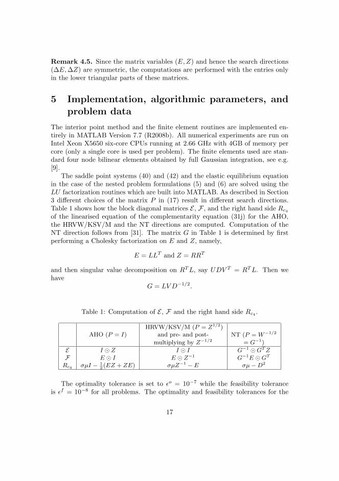
The saddle point systems (40) and (42) and the elastic equilibrium equationin the case of the nested problem formulations (5) and (6) are solved using theLU factorization routines which are built into MATLAB. As described in Section3 different choices of the matrix P in (17) result in different search directions.Table 1 shows how the block diagonal matrices E , F , and the right hand side Rc4of the linearised equation of the complementarity equation (31j) for the AHO,the HRVW/KSV/M and the NT directions are computed. Computation of theNT direction follows from [31]. The matrix G in Table 1 is determined by firstperforming a Cholesky factorization on E and Z, namely,

E = LLT and Z = RRT

and then singular value decomposition on RTL, say UDV T = RTL. Then wehave

G = LV D−1/2.

Table 1: Computation of E , F and the right hand side Rc4 .

AHO (P = I)HRVW/KSV/M (P = Z1/2)

NT (P = W−1/2and pre- and post-

multiplying by Z−1/2 = G−1)

E I Z I I G−1 GTZF E I E Z−1 G−1E GT

Rc4 σµI − 12(EZ + ZE) σµZ−1 − E σµ−D2

The optimality tolerance is set to εo = 10−7 while the feasibility toleranceis εf = 10−8 for all problems. The optimality and feasibility tolerances for the

17

barrier problems are computed as in (26). We say that the current iterate is asolution if it satisfies the stopping criteria for the inner and outer iterations asoutlined in (25) and (24). The minimum barrier parameter value µmin is set to10−9. The boundary to the fraction parameter τ is set to 0.9. The parametersused in the backtracking line search are set as η = 0.5 and τ0 = 10−5, respectively.For all problems we observe that the algorithm converges without performingany line search. This could be because the treated problems are either convexor can be equivalently written as a convex problem. For this reason the linesearch part of the algorithm was not activated in the numerical experiments.Both barrier update strategies given in (27) and (28) are implemented. In thenumerical experiments we use (27) with σ = 0.4 since the µ values in this caseare proportional to the duality gap.

The primal design variables are initially set to Ei = 0.1ρI for all i, while theprimal displacement variables are set to zero, i.e. u` = 0 for all `. All slack vari-ables are all set to ones and that Lagrange multipliers for equality constraints areset to zero. Lagrange multipliers for scalar (or matrix) inequalities are otherwiseset to ones (or identity matrices). When solving minimum compliance problemsthe total weight fraction is set to 33.3% of the maximum weight, i.e. V = (m/3)ρ.When solving the minimum weight problems the bound on the compliance is setto 25% of the compliance evaluated at the initial point. The local bounds on theTr(Ei) are scaled in such away that ρ/ρ = 104.

6 Numerical experiments

The numerical experiments have three objectives. The first goal is to comparethe performance of the interior point method when applied to the different FMOformulations presented in Section 2 and determine the best choice of formula-tion. The second goal is to investigate the numerical behaviour of the AHO,the HRVW/KSV/M, and the NT search directions and give recommendations.We use performance profiles as introduced in [10] to evaluate the numerical per-formances. The number of iterations and CPU time of the method required toobtain a solution are used as measures of the performances. The third goal is toshow the efficiency of the method. This is achieved first by reporting solutionsto a set of large-scale FMO problems. Second, by solving benchmark problemsand making comparison to the recent numerical results presented in [29]. Theresults in [29] are obtained using a state-of-the-art special purpose method forFMO problems.

Throughout the article we use the colour bar in Figure 1 to show the optimaldensity distribution, that is, the trace of the stiffness tensor of the optimal designs.

18

ρ ρ

Figure 1: Colour bar for the optimal density distribution.

6.1 Performance

We consider a set of FMO problem instances over 2D design domains to comparethe performance of the formulations and search directions. Four two-dimensionalbenchmark problems from [37], [7], and [19] are considered. The design domains,boundary conditions, and loads for these problems are shown in Figure 2. Thefirst one is a single load Cantilever beam problem with design domain dimensions2 × 1. The second problem is a single load Michell beam problem with designdomain dimensions 2 × 1. In the third problem we consider an L-shaped designdomain with dimension 1 × 1 with a quarter square removed from one corner.The last benchmark is a two load problem with a rectangular design domain ofdimension 2× 1. In all cases we apply a load over a segment of length 0.04. Foreach design domain there are four level of finite element discretizations with thefiner mesh obtained from the coarser by refining each element into four elements.Details of the problem instances are given in Table 2.

6.1.1 Performance of the formulations

Considering the minimum compliance problem we solve the three formulations,namely, the simultaneous analysis and design approach (3), the dual formula-tion (8), and the nested approach (5) for all problem instances in Table 2. Itis shown in Figure 5 that the performance profiles are similar. The identicalprofiles of the dual and SAND formulations in Figure 5a is the result of the sim-ilarity (up to a scaling) of the optimality conditions (once λ is eliminated fromthe optimality condition of the SAND formulation to get (32)). While solvingthe nested formulation the additional computational effort of solving the elasticequilibrium equations as in the second part of (37) at each interior point iterationis almost not visible in the performance profiles. It is slightly more noticeable forthe multiple load case problems. For example, for solving the minimum weightproblem on the ”Two Loads Case IV” in Table 2, the average CPU time spenton one interior point iteration was 453 seconds for solving the problem of SANDformulation and 465 seconds for the problem of nest formulation. We expecthigher computational efforts if we solve much larger problems or problems over3D design domains. For the minimum weight problem we solve the simultaneous

19

(a) (b)

(c) (d)

Figure 2: Design domains, boundary conditions, and external loads for the Can-tilever benchmark problem (a), the Michell beam problem (b), the L-shape prob-lem (c), and the two load case problem (d).

20

(a) (b)

(c) (d)

Figure 3: Optimal density distribution obtained by solving the minimum com-pliance problem (3) for the Cantilever IV benchmark problem (a), the MichellIV beam problem (b), the L-shape IV problem (c), and the two load case IVproblem (d).

(a) (b)

Figure 4: Principal material directions for the optimal designs for the Michellbeam problem (a), and the two load case problem (b).

21

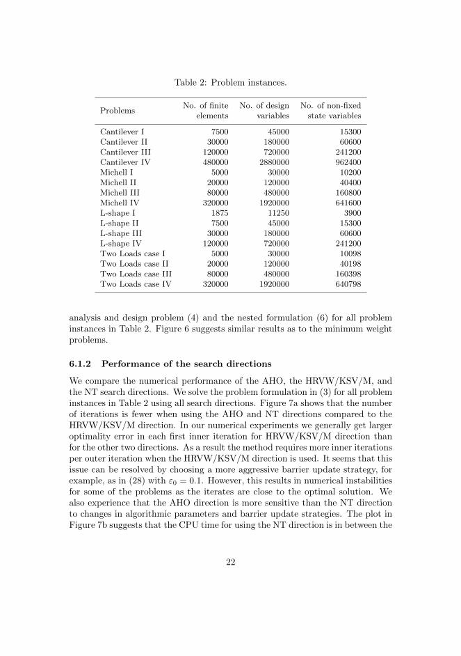
Table 2: Problem instances.

ProblemsNo. of finite No. of design No. of non-fixed

elements variables state variables

Cantilever I 7500 45000 15300Cantilever II 30000 180000 60600Cantilever III 120000 720000 241200Cantilever IV 480000 2880000 962400Michell I 5000 30000 10200Michell II 20000 120000 40400Michell III 80000 480000 160800Michell IV 320000 1920000 641600L-shape I 1875 11250 3900L-shape II 7500 45000 15300L-shape III 30000 180000 60600L-shape IV 120000 720000 241200Two Loads case I 5000 30000 10098Two Loads case II 20000 120000 40198Two Loads case III 80000 480000 160398Two Loads case IV 320000 1920000 640798

analysis and design problem (4) and the nested formulation (6) for all probleminstances in Table 2. Figure 6 suggests similar results as to the minimum weightproblems.

6.1.2 Performance of the search directions

We compare the numerical performance of the AHO, the HRVW/KSV/M, andthe NT search directions. We solve the problem formulation in (3) for all probleminstances in Table 2 using all search directions. Figure 7a shows that the numberof iterations is fewer when using the AHO and NT directions compared to theHRVW/KSV/M direction. In our numerical experiments we generally get largeroptimality error in each first inner iteration for HRVW/KSV/M direction thanfor the other two directions. As a result the method requires more inner iterationsper outer iteration when the HRVW/KSV/M direction is used. It seems that thisissue can be resolved by choosing a more aggressive barrier update strategy, forexample, as in (28) with ε0 = 0.1. However, this results in numerical instabilitiesfor some of the problems as the iterates are close to the optimal solution. Wealso experience that the AHO direction is more sensitive than the NT directionto changes in algorithmic parameters and barrier update strategies. The plot inFigure 7b suggests that the CPU time for using the NT direction is in between the

22

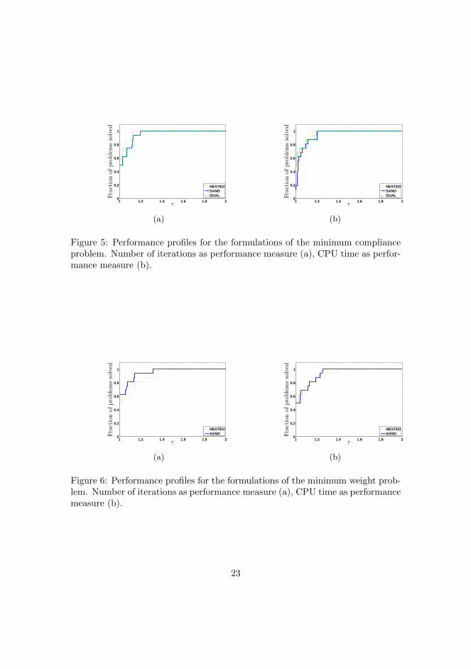
1 1.2 1.4 1.6 1.8 20

0.2

0.4

0.6

0.8

1

τ

Fractionofproblemssolved

NESTEDSANDDUAL

(a)

1 1.2 1.4 1.6 1.8 20

0.2

0.4

0.6

0.8

1

τ

Fractionofproblemssolved

NESTEDSANDDUAL

(b)

Figure 5: Performance profiles for the formulations of the minimum complianceproblem. Number of iterations as performance measure (a), CPU time as perfor-mance measure (b).

1 1.2 1.4 1.6 1.8 20

0.2

0.4

0.6

0.8

1

τ

Fractionofproblemssolved

NESTEDSAND

(a)

1 1.2 1.4 1.6 1.8 20

0.2

0.4

0.6

0.8

1

τ

Fractionofproblemssolved

NESTEDSAND

(b)

Figure 6: Performance profiles for the formulations of the minimum weight prob-lem. Number of iterations as performance measure (a), CPU time as performancemeasure (b).

23

1 1.5 2 2.5 3 3.5 4 4.5 50

0.2

0.4

0.6

0.8

1

τ

Fractionofproblemssolved

AHOHRVW/KSV/MNT

(a)

1 1.5 2 2.5 3 3.5 4 4.5 50

0.2

0.4

0.6

0.8

1

τ

Fractionofproblemssolved

AHOHRVW/KSV/MNT

(b)

Figure 7: Performance profiles for the search directions. Number of iterations asperformance measure (a), CPU time as performance measure (b).

AHO and the HRVW/KSV/M directions. This is because we perform Choleskyfactorizations of each Ei and Zi for i = 1, . . . ,m and the additionally the SingularValue Decompositions of a matrix computed from the Cholesky factorizations.

The plots for the optimal density distribution of each design domain is givenin Figure 3. The principal material directions of optimal designs for the Michellbeam and the two load case problems are shown in Figure 4. The directions arecomputed based on the principal eigenvectors associated to the Voigt-stiffnesstensor. The numerical result for solving problem (3) for each problem instancesin Table 2 is given in Table 3.

6.2 Efficiency compared to alternative methods

The problems listed in Table 3 are, by far, the largest FMO problems reportedto date. The proposed primal-dual interior point method requires a modestnumber of iterations. All problem instances reported in Table 3 are solved within25-55 iterations. Table 3 illustrates that there is a mild increase in number ofiterations with increasing problem size. We also notice that when solving thelargest problems the memory requirements and the computational expense of themethod are largely dominated by the solution of the saddle point system (42)and additionally of the elastic equilibrium equation for the nested formulations.

We also make comparisons with the FMO results presented in [29]. The prob-lems in [29] are solved by the code PENSCP. At present the comparison is limitedonly to problems considered in this article. The comparison is indeed merely ina sense that we solve a multiple load case of problem formulation (5) while in[29] an alternative worst-case multiple problem is solved. Moreover, the loadingand the size of fixed boundary regions could differ up to scaling. Comparisonon CPU time also have discrepancy for the fact that the programming languages

24

Table 3: Numerical results for the problem instances in Table 2 and the minimumcompliance problem (3).

Problems No. of iterations CPU time (s) Compliance

Cantilever I 34 213 5.0816Cantilever II 44 1128 5.0802Cantilever III 40 4257 5.0826Cantilever IV 40 17713 5.0925Michell I 34 142 1.8331Michell II 48 819 1.8349Michell III 55 3809 1.8362Michell IV 49 13787 1.8391L-shape I 29 47 2.1780L-shape II 35 215 2.1814L-shape III 35 896 2.1845L-shape IV 34 3518 2.1885Two Loads case I 25 134 0.4220Two Loads case II 28 622 0.4253Two Loads case III 30 2941 0.4263Two Loads case IV 31 14441 0.4272

and the machines used to perform numerical experiments are different. However,the reported results are still interesting since the efficiency both in CPU time andnumber of iterations required to get even a higher quality solution is significant.The design domain, boundary conditions, and loads are depicted in Figure 8. InTable 4 we report the numerical results for a four load case with three differentdiscretizations. In the first column we list the number of finite elements, in thesecond column the number of iterations, in the third column the achieved op-timality and feasibility tolerances, and in the fourth column the CPU time. Inthe fifth and sixth columns we include the number of iterations and the CPUtime from [29] required by PENSCP to solve the problem. Note that the CPUtimes reported include the entire computation process, i.e, starting from meshand finite element generations to the end of the optimization process. When wecompare the obtained results to the results in Table 7.1 in [29], we notice thatthe efficiency of the proposed interior point method both in time and number ofiteration. The solutions obtained with the interior point method are also moreaccurate. In [29] one of the stopping criteria used is a measure of the optimalityerror that is set to lower tolerance than used in our numerical experiment. Wealso solve another problem with 5000 elements for three different load cases. Thenumerical result is presented in Table 5. In this table the first column containsthe load cases and the other columns are similar to those of Table 4. This table

25

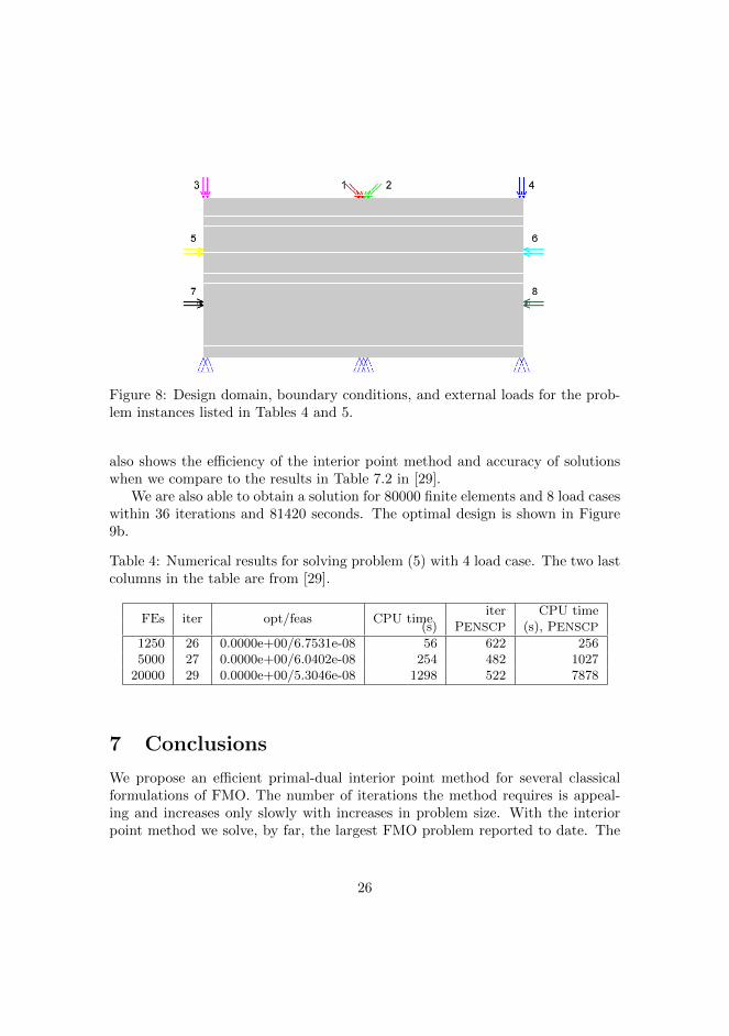
Figure 8: Design domain, boundary conditions, and external loads for the prob-lem instances listed in Tables 4 and 5.

also shows the efficiency of the interior point method and accuracy of solutionswhen we compare to the results in Table 7.2 in [29].

We are also able to obtain a solution for 80000 finite elements and 8 load caseswithin 36 iterations and 81420 seconds. The optimal design is shown in Figure9b.

Table 4: Numerical results for solving problem (5) with 4 load case. The two lastcolumns in the table are from [29].

FEs iter opt/feas CPU timeiter CPU time

(s) PENSCP (s), PENSCP

1250 26 0.0000e+00/6.7531e-08 56 622 2565000 27 0.0000e+00/6.0402e-08 254 482 1027

20000 29 0.0000e+00/5.3046e-08 1298 522 7878

7 Conclusions

We propose an efficient primal-dual interior point method for several classicalformulations of FMO. The number of iterations the method requires is appeal-ing and increases only slowly with increases in problem size. With the interiorpoint method we solve, by far, the largest FMO problem reported to date. The

26

(a) (b)

Figure 9: Optimal density distribution for the multiple load problem in Figure8. Problem with 20000 finite elements and 4 load cases as described in Tables 4and 5 (a), problem with 80000 finite elements and 8 load cases (b).

Table 5: Numerical results for solving problem (5). The design domain is par-titioned into 5000 finite elements. The two last columns in the table are from[29].

Lc iter opt/feas CPU time (s)iter CPU time (s)

PENSCP PENSCP

2 31 0.0000e+00/1.2200e-08 166 543 5854 27 0.0000e+00/6.0402e-08 245 489 10278 28 0.0000e+00/2.7303e-08 738 370 1319

obtained accuracy of the computed optimal solutions is higher compared to so-lutions obtained by other methods developed for FMO. For large-scale problemsthe memory requirements and the computation time of the method are domi-nated by the direct solution of the saddle point systems for computing the searchdirection. Future research will be directed towards developments of efficient pre-conditioner for iterative methods for the saddle-point systems with the aim tosolve very large-scale 3D problems.

The number of iterations of the method is similar when solving either of thesimultaneous analysis and design or the nested problem formulations. For solvingthe nested problem formulation the additional expected computational effort ofsolving the elastic equilibrium equations at each interior point iteration is almostnot visible for the problems sizes considered. However, the differences that canbe seen when solving multiple load problems could indicate higher computationalefforts if we solve much larger problems or problems over 3D design domains. Thedual formulation (8) also works well. However, there are no dual reformulationslike (8) if other constraints, such as stress constraints, are included in the problem

27

formulations.Our numerical experiments indicate that the NT and AHO directions are more

efficient than the HRVW/KSV/M direction as they require fewer inner iterationsper outer iteration. Comparing the AHO and NT directions we experience thatthe NT directions are less sensitive to changes in algorithmic parameters andspeed of updating the barrier parameter. Therefore, the NT direction is ourpreferred choice.

The results in this article are exclusively supported by numerical experiments.Theoretical treatment of convergence theory of the interior point method must befurther analysed. The applicability of relevant available theories in the literatureshould be investigated and potentially applied to show global convergence.

8 Acknowledgements

The authors would like to thank two reviewers for their constructive and insightfulcomments and suggestions. We also would like to express our gratitude to ourformer colleague Stefanie Gaile for many and fruitful discussions on Free MaterialOptimization.

The research was partially funded by the Danish Council for Strategic Re-search through the Danish Center for Composite Structures and Materials (DCCSM).

References

[1] Achtziger, W., Bendsøe, M., Ben-Tal, A., Zowe, J.: Equivalent displacementbased formulations for maximum strength truss topology design. Impact ofComputing in Science and Engineering 4, 315–345 (1992)

[2] Alizadeh, F., Haeberly, J., Overton, M.: Primal-dual interior-point methodsfor semidefinite programming: convergence rates, stability and numericalresults. SIAM Journal on Optimization 8(3), 746–768 (2009)

[3] Ben-Tal, A., Kocvara, M., Nemirovski, A., Zowe, J.: Free material designvia semidefinite programming: The multiload case with contact conditions.SIAM Journal on Optimization 9(4), 813–832 (1999)

[4] Ben-Tal, A., Nemirovski, A.: Robust truss topology design via semidefiniteprogramming. SIAM Journal on Optimization 7(4), 991–1016 (1997)

[5] Ben-Tal, A., Nemirovski, A.: Handbook of semidefinite programming, chap.Structural Design, pp. 443–467. Kluwer Academic Publishers (2000)

28

[6] Bendsøe, M., Dıaz, A.: Optimization of material properties for Mindlin platedesign. Structural Optimization 6, 268–270 (1993)

[7] Bendsøe, M., Guedes, J., Haber, R., Pedersen, P., Taylor, J.: An analyti-cal model to predict optimal material properties in the context of optimalstructural design. Journal of Applied Mechanics 61, 930–937 (1994)

[8] Benson, H., Shanno, D.: Interior-point methods for nonconvex nonlinearprogramming: regularization and warmstarts. Computational Optimizationand Applications 40, 143–189 (2008)

[9] Cook, R., Malkus, D., Plesha, M., Witt, R.: Concepts and Applications ofFinite Element Analysis, 4th edn. John Wiley and Sons (2002)

[10] Dolan, E., More, J.: Benchmarking optimization software with performanceprofiles. Mathematical Programming 97(A), 201–213 (2002)

[11] Forsgren, A., Gill, P.: Primal-dual interior methods for nonconvex nonlinearprogramming. SIAM Journal on Optimization 8(4), 1132–1152 (1998)

[12] Forsgren, A., Gill, P., Wright, M.: Interior methods for nonlinear optimiza-tion. SIAM Review 44(4), 525–597 (2002)

[13] Gaile, S.: Free material optimization for shells and plates. Ph.D. thesis, Insti-tute of Applied Mathematics II, Friedrich-Alexander University of Erlangen-Nuremberg (2011)

[14] Golub, G., van Loan, C.: Matrix Computations, 3rd edn. Johns HopkinsUniversity Press (1996)

[15] Haslinger, J., Kocvara, M., Leugering, G., Stingl, M.: Multidisciplinary freematerial optimization. SIAM Journal on Applied Mathematics 70(7), 2709–2728 (2010)

[16] Helmberg, C., Rendl, F., Vanderbei, R., Wolkowicz, H.: An interior-pointmethod for semidefinite programming. SIAM Journal on Optimization 6,342–361 (1996)

[17] Kojima, M., Shindoh, S., Hara, S.: Interior-point methods for the monotonesemidefinite linear complementarity problem in symmetric matrices. SIAMJournal on Optimization 7(1), 86–125 (1997)

[18] Kocvara, M., Stingl, M.: PENNON A code for convex nonlinear and semidef-inite programming. Optimization Methods and Software 18(3), 317–333(2003)

29

[19] Kocvara, M., Stingl, M.: Free material optimization for stress constraints.Structural and Multidisciplinary Optimization 33, 323–335 (2007)

[20] Kocvara, M., Stingl, M., Zowe, J.: Free material optimization: recentprogress. Optimization 57(1), 79–100 (2008)

[21] Monteiro, R.: Primal-dual path-following algorithms for semidefinite pro-gramming. SIAM Journal on Optimization 7(3), 663–678 (1997)

[22] Monteiro, R.: First- and second-order methods for semidefinite program-ming. Mathematical Programming 97, 209–244 (2003)

[23] Nesterov, Y., Todd, M.: Self-scaled barriers and interior-point methods forconvex programming. Mathematics of Operations Research 22(1), 1–42(1997)

[24] Nesterov, Y., Todd, M.: Primal-dual interior-point methods for self-scaledcones. SIAM Journal on Optimization 8(2), 324–364 (1998)

[25] Ringertz, U.: On finding the optimal distribution of material properties.Structural Optimization 5, 265–267 (1993)

[26] Stingl, M.: On the solution of nonlinear semidefinite programs by augmentedLagrangian method. Ph.D. thesis, Institute of Applied Mathematics II,Friedrich-Alexander University of Erlangen-Nuremberg (2006)

[27] Stingl, M., Kocvara, M., Leugering, G.: Free material optimization withfundamental eigenfrequency constraints. SIAM Journal on Optimization20(1), 524–547 (2009)

[28] Stingl, M., Kocvara, M., Leugering, G.: A new non-linear semidefinite pro-gramming algorithm with an application to multidisciplinary free materialoptimization. International Series of Numerical Mathematics 158, 275–295(2009)

[29] Stingl, M., Kocvara, M., Leugering, G.: A sequential convex semidefiniteprogramming algorithm with an application to multiple-load free materialoptimization. SIAM Journal on Optimization 20(1), 130–155 (2009)

[30] Todd, M.: A study of search directions in primal-dual interior-point methodsfor semidefinite programming. Optmization Methods and Software 11, 1–46(1999)

[31] Todd, Y., Toh, K., Tutuncu, R.: On the Nesterov-Todd direction in semidef-inite programming. SIAM Journal on Optimization 8(3), 769–796 (1998)

30

[32] Vogelbusch, C.H.: Numerical treatment of nonlinear semidefinite pro-grams. Ph.D. thesis, Institut fur Mathematik der Heinrich-Heine-UniversitatDusseldorf (2006)

[33] Waltz, R., Morales, J., Nocedal, J., Orban, D.: An interior algorithm fornonlinear optimization that combines line search and trust region steps.Mathematical Programming 107, 391–408 (2006)

[34] Werner, R.: Free material optimization-mathematical analysis and numer-ical solution. Ph.D. thesis, Institute of Applied Mathematics II, Friedrich-Alexander University of Erlangen-Nuremberg (2001)

[35] Yamashita, H., Yabe, H., Harada, K.: A primal-dual interior point methodfor nonlinear semidefinite programming. Mathematical Programming 135,89–121 (2012)

[36] Zhang, Y.: On extending some primal-dual interior-point algorithms fromlinear programming to semidefinite programming. SIAM Journal on Opti-mization 8(2), 365–386 (1998)

[37] Zowe, J., Kocvara, M., Bendsøe, M.: Free material optimization via mathe-matical programming. Mathematical Programming 79, 445–466 (1997)

Appendix A

In this Appendix we derive the dual formulation (8) of the minimum weightedcompliance problem (3). Similar result for minimax problems can be found in[3]. Analogous all-quadratic formulations of minimum compliance truss topologyoptimization problems are described, for example, in [1]. The linear elasticitystatic structural analysis problem can be written as

supu`

2fT` u` − uT` A(E)u`

which is a quadratic problem with negative definite Hessian and hence a concavemaximization problem. The optimality condition is A(E)u` = f` and the optimalvalue is fT` u` if f` ∈ R(A(E)) and −∞ otherwise. Due to the stated assumptionswe replace the sup with max in the following. Therefore, the minimum compliance

31

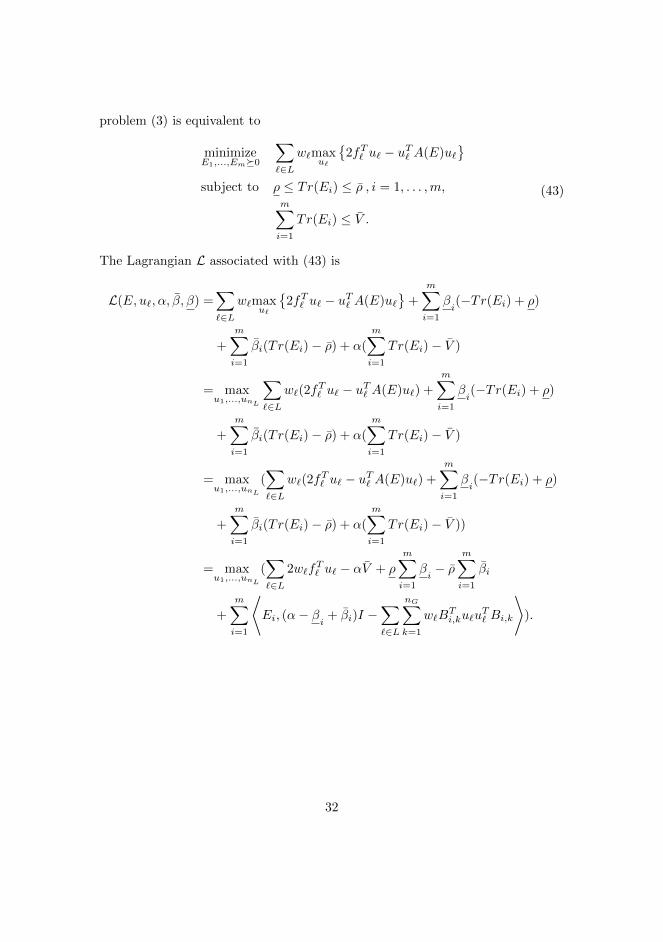
problem (3) is equivalent to

minimizeE1,...,Em0

∑

`∈Lw`max

u`

2fT` u` − uT` A(E)u`

subject to ρ ≤ Tr(Ei) ≤ ρ , i = 1, . . . ,m,m∑

i=1

Tr(Ei) ≤ V .

(43)

The Lagrangian L associated with (43) is

L(E, u`, α, β, β) =∑

`∈Lw`max

u`

2fT` u` − uT` A(E)u`

+

m∑

i=1

βi(−Tr(Ei) + ρ)

+m∑

i=1

βi(Tr(Ei)− ρ) + α(m∑

i=1

Tr(Ei)− V )

= maxu1,...,unL

∑

`∈Lw`(2f

T` u` − uT` A(E)u`) +

m∑

i=1

βi(−Tr(Ei) + ρ)

+m∑

i=1

βi(Tr(Ei)− ρ) + α(m∑

i=1

Tr(Ei)− V )

= maxu1,...,unL

(∑

`∈Lw`(2f

T` u` − uT` A(E)u`) +

m∑

i=1

βi(−Tr(Ei) + ρ)

+

m∑

i=1

βi(Tr(Ei)− ρ) + α(

m∑

i=1

Tr(Ei)− V ))

= maxu1,...,unL

(∑

`∈L2w`f

T` u` − αV + ρ

m∑

i=1

βi− ρ

m∑

i=1

βi

+m∑

i=1

⟨Ei, (α− βi + βi)I −

∑

`∈L

nG∑

k=1

w`BTi,ku`u

T` Bi,k

⟩).

32

The corresponding dual function is

g(u1, . . . , unL , β, β, α)

= minimizeE1,...,Em0

maxu1,...,unL

(∑

`∈L2w`f

T` u` − αV + ρ

m∑

i=1

βi− ρ

m∑

i=1

βi

+

m∑

i=1

⟨Ei, (α− βi + βi)I −

∑

`∈L

nG∑

k=1

w`BTi,ku`u

T` Bi,k

⟩)

=

max

u1,...,unL(∑`∈L 2w`f

T` u` − αV + ρ

∑mi=1 βi − ρ

∑mi=1 βi) if (44) holds

−∞ otherwise.

Below is the condition that the dual function g attains its minimum value.

∑

`∈L

nG∑

k=1

w`BTi,ku`u

T` Bi,k (α− β

i+ βi)I, i = 1, . . . ,m. (44)

The dual formulation of the minimum compliance problem (3) becomes

supu1,...,unL ,α≥0,β≥0,β≥0

− αV + 2∑

`∈Lw`f

T` u` + ρ

m∑

i=1

βi− ρ

m∑

i=1

βi

subject to∑

`∈L

nG∑

k=1

w`BTi,ku`u

T` Bi,k − (α− β

i+ βi)I 0 , i = 1, . . . ,m.

Appendix B

The following products are in tensor notation.

1. (∇2XrXs

Lµ(X,u, s, λ)∆Xs)ij = (∇2XrXs

Lµ(X,u, s, λ))ijpq(∆Xs)pq, for r, s =1, ..,m, for i, j = 1, ..., dr, and for p, q = 1, ..., ds.

2. (∇2XruLµ(X,u, s, λ)∆Xr)i = (∇2

uXrLµ(X,u, s, λ))ipq(∆Xr)pq, for r = 1, ..,m,

for p, q = 1, ..., dr, and for i = 1, ..., n.

3. (∇2XruLµ(X,u, s, λ)T∆u)ij = (∇2

XruLµ(X,u, s, λ))ijp(∆u)p, for r = 1, ..,m,

for i, j = 1, ..., dr, and for p = 1, ..., n.

4. (∇Xrg(X,u)T∆λ)ij = (∇Xr (g(X,u)T∆λ))ij , for r = 1, ..,m, and for i, j =1, ..., dr.

5. (∇Xrg(X,u)∆Xr)i = (∇Xrgi(X,u))pq(∆Xr)pq, for r = 1, ..,m, for p, q =1, ..., dr, and for i = 1, ..., k.

33

Chapter 6

Free Material Optimizationfor Laminated Plates andShells

Accepted in 2014 and in print:Weldeyesus, A.G., Stolpe, M.: Free Material Optimization for Laminated Platesand Shells. Journal of Structural and Multidisciplinary Optimization.

56

Free Material Optimization for Laminated Plates

and Shells

Alemseged Gebrehiwot Weldeyesus∗ and Mathias Stolpe†

Abstract

Free Material Optimization (FMO) is a powerful approach for concep-tual optimal design of composite structures. The design variable in FMO isthe entire elastic material tensor which is allowed to vary almost freely overthe design domain. The imposed requirements on the tensor are that it issymmetric and positive semidefinite. Most of today’s studies on FMO focuson models for two- and three-dimensional structures. The objective of thisarticle is to extend existing FMO models and methods to laminated plateand shell structures, which are used in many engineering applications. InFMO, the resulting optimization problem is generally a non convex semidef-inite program with many small matrix inequalities which requires special-purpose optimization methods. The FMO problems are efficiently solvedby a primal-dual interior point method developed and implemented by theauthors. The quality of the proposed FMO models and the method aresupported by several large-scale numerical experiments.

Mathematics Subject Classification 2010: 90C22, 90C90, 74P05, 74P15

Keywords: Structural optimization, free material optimization, nonlinear semidef-inite optimization, laminated shells

The research was partially funded by the Danish Council for Strategic Research throughthe Danish Center for Composite Structures and Materials (DCCSM) and the Danish Councilfor Independent Research — Technology and Production Sciences through the research projectOptimal Design of Composite Structures under Manufacturing Constraints.∗DTU Wind Energy, Technical University of Denmark, Frederiksborgvej 399, 4000 Roskilde,

Denmark. E-mail: alwel@dtu.dk†DTU Wind Energy, Technical University of Denmark, Frederiksborgvej 399, 4000 Roskilde,

Denmark. E-mail: matst@dtu.dk

1

1 Introduction

In Free Material Optimization (FMO) the design parametrization allows completecontrol over the entire material tensor. It is allowed vary freely at each point ofthe design domain with the only requirement that it has to satisfy mild necessaryconditions for physical attainability. Therefore, in optimal structures obtainedby FMO both the distribution of the amount of material and the optimal localmaterial properties are determined.

The basic concept of FMO was introduced in the early 1990s in [3], [4], and[22]. Since then, several studies led to the development of models, theories, andnumerical methods for FMO problems. In the recently proposed FMO prob-lems several types of constraints have been introduced. For example in [15],[14], and [10] problems with constraints on local stresses and displacements andin [26] problems with constraints on fundamental eigenfrequencies are presentedand solved. Some of the studies not only emphasize on extending the formula-tions to multidisciplinary problems but also on development of new optimizationmethods. The methods include a method based on penalty/barrier multipliers(PBM) in [33] and a method based an augmented Lagrangian function in [13]and [25]. Recently a method based on a sequential convex programming concept[28, 27] and a method based on interior point methods [29] were proposed forFMO. Moreover, detailed theory covering choice of problem formulations and theexistence of solutions can be found in [30].

Most of today’s FMO studies focus on two- and three-dimensional designdomains. In this article we focus on laminated plates and shells which nowa-days are used in many engineering applications. There are several approachesto material optimization of such structures. One of them is Discrete MaterialOptimization (DMO) which was introduced in [23], [24], and [17]. DMO de-termines the best discrete material selection, stacking sequence, and thicknessdistribution. An FMO model for Mindlin plate design is introduced in [3]. Laterin [9] FMO formulations, analogous to the recent FMO formulations for two- andthree-dimensional structures, are proposed for single layer plates and shells. Asfar as to our knowledge, no FMO models have been proposed for general lam-inated shell structures. Therefore, we propose new FMO models for laminatedplates and shells by extending the formulations in [9].

The requirement of physical attainability of the elastic stiffness tensor leadsto a mathematical interpretation that the stiffness tensor must be symmetricpositive semidefinite. For this reason, FMO problems result in an optimizationproblem that belongs to the class of nonlinear semidefinite programming (SDP).We generalize the primal-dual interior point method proposed by the authorsin [29] which is especially developed for FMO problems. The method and itsimplementation exploit the property that FMO problems have many matrix in-

2

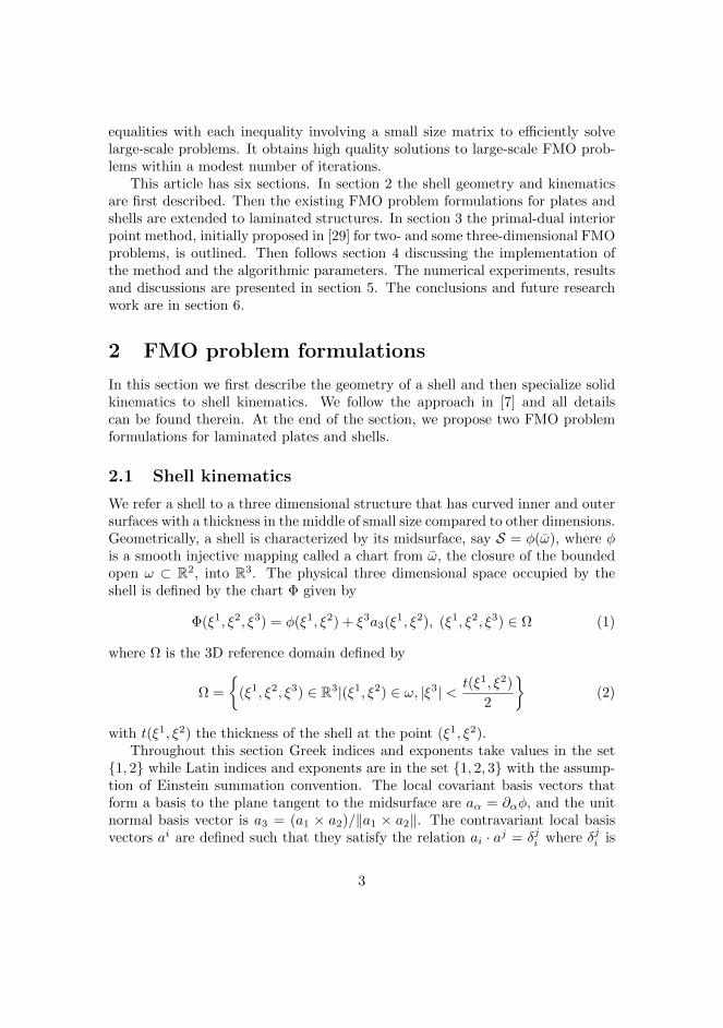
equalities with each inequality involving a small size matrix to efficiently solvelarge-scale problems. It obtains high quality solutions to large-scale FMO prob-lems within a modest number of iterations.

This article has six sections. In section 2 the shell geometry and kinematicsare first described. Then the existing FMO problem formulations for plates andshells are extended to laminated structures. In section 3 the primal-dual interiorpoint method, initially proposed in [29] for two- and some three-dimensional FMOproblems, is outlined. Then follows section 4 discussing the implementation ofthe method and the algorithmic parameters. The numerical experiments, resultsand discussions are presented in section 5. The conclusions and future researchwork are in section 6.

2 FMO problem formulations

In this section we first describe the geometry of a shell and then specialize solidkinematics to shell kinematics. We follow the approach in [7] and all detailscan be found therein. At the end of the section, we propose two FMO problemformulations for laminated plates and shells.

2.1 Shell kinematics

We refer a shell to a three dimensional structure that has curved inner and outersurfaces with a thickness in the middle of small size compared to other dimensions.Geometrically, a shell is characterized by its midsurface, say S = φ(ω), where φis a smooth injective mapping called a chart from ω, the closure of the boundedopen ω ⊂ R2, into R3. The physical three dimensional space occupied by theshell is defined by the chart Φ given by

Φ(ξ1, ξ2, ξ3) = φ(ξ1, ξ2) + ξ3a3(ξ1, ξ2), (ξ1, ξ2, ξ3) ∈ Ω (1)

where Ω is the 3D reference domain defined by

Ω =

(ξ1, ξ2, ξ3) ∈ R3|(ξ1, ξ2) ∈ ω, |ξ3| < t(ξ1, ξ2)

2

(2)

with t(ξ1, ξ2) the thickness of the shell at the point (ξ1, ξ2).Throughout this section Greek indices and exponents take values in the set

1, 2 while Latin indices and exponents are in the set 1, 2, 3 with the assump-tion of Einstein summation convention. The local covariant basis vectors thatform a basis to the plane tangent to the midsurface are aα = ∂αφ, and the unitnormal basis vector is a3 = (a1 × a2)/‖a1 × a2‖. The contravariant local basisvectors ai are defined such that they satisfy the relation ai · aj = δji where δji is

3

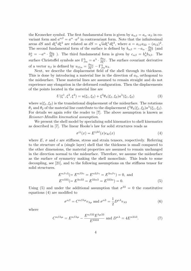
the Kronecker symbol. The first fundamental form is given by aαβ = aα ·aβ in co-variant form and aαβ = aα ·aβ in contravariant form. Note that the infinitesimalareas dS and dξ1dξ2 are related as dS =

√adξ1dξ2, where a = a11a22 − (a12)2.

The second fundamental form of the surface is defined by bαβ = −aα · ∂a3∂ξβ(and

bαβ = −aα · ∂a3∂ξβ

). The third fundamental form is given by cαβ = bλαbλβ . The

surface Christoffel symbols are Γλβα = aλ · ∂aβ∂ξα . The surface covariant derivative

of a vector uβ is defined by uβ|α =∂uβ∂ξα − Γλβαuλ.

Next, we describe the displacement field of the shell through its thickness.This is done by introducing a material line in the direction of a3, orthogonal tothe midsurface. These material lines are assumed to remain straight and do notexperience any elongation in the deformed configuration. Then the displacementsof the points located in the material line are

U(ξ1, ξ2, ξ3) = u(ξ1, ξ2) + ξ3θλ(ξ1, ξ2)aλ(ξ1, ξ2) (3)

where u(ξ1, ξ2) is the translational displacement of the midsurface. The rotationsθ1 and θ2 of the material line contribute to the displacement ξ3θλ(ξ1, ξ2)aλ(ξ1, ξ2).For details we again refer the reader to [7]. The above assumption is known asReissner-Mindlin kinematical assumption.

We present the shell model by specializing solid kinematics to shell kinematicsas described in [7]. The linear Hooke’s law for solid structures reads as

σij(x) = Eijkl(x)ekl(x) (4)

where E, σ and e are stiffness, stress and strain tensors, respectively. Referringto the structure of a (single layer) shell that the thickness is small compared tothe other dimensions, the material properties are assumed to remain unchangedin the direction normal to the midsurface. Therefore, we assume the midsurfaceas the surface of symmetry making the shell monoclinic. This leads to somedecoupling, see [21], and to the following assumptions on the stiffness tensor forsolid structures.

Eαβγ3(= Eαβ3γ = Eα3βγ = E3αβγ) = 0, and

Eα333(= E3α33 = E33α3 = E333α) = 0. (5)

Using (5) and under the additional assumption that σ33 = 0 the constitutiveequations (4) are modified to

σαβ = Cαβλµeλµ and σα3 =1

2Dαλeλ3 (6)

where

Cαβλµ = Eαβλµ − Eαβ33Eλµ33

E3333and Dαλ = 4Eα3λ3. (7)

4

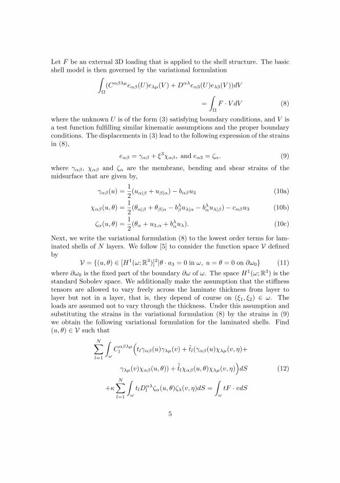
Let F be an external 3D loading that is applied to the shell structure. The basicshell model is then governed by the variational formulation

∫

Ω

(Cαβλµeαβ(U)eλµ(V ) +Dαλeα3(U)eλ3(V ))dV

=

∫

Ω

F · V dV (8)

where the unknown U is of the form (3) satisfying boundary conditions, and V isa test function fulfilling similar kinematic assumptions and the proper boundaryconditions. The displacements in (3) lead to the following expression of the strainsin (8),

eαβ = γαβ + ξ3χαβ , and eα3 = ζα. (9)

where γαβ , χαβ and ζα are the membrane, bending and shear strains of themidsurface that are given by,

γαβ(u) =1

2(uα|β + uβ|α)− bαβu3 (10a)

χαβ(u, θ) =1

2(θα|β + θβ|α − bλβuλ|α − bλαuλ|β)− cαβu3 (10b)

ζα(u, θ) =1

2(θα + u3,α + bλαuλ). (10c)

Next, we write the variational formulation (8) to the lowest order terms for lam-inated shells of N layers. We follow [5] to consider the function space V definedby

V = (u, θ) ∈ [H1(ω;R3)]2|θ · a3 = 0 in ω, u = θ = 0 on ∂ω0 (11)

where ∂ω0 is the fixed part of the boundary ∂ω of ω. The space H1(ω;R3) is thestandard Sobolev space. We additionally make the assumption that the stiffnesstensors are allowed to vary freely across the laminate thickness from layer tolayer but not in a layer, that is, they depend of course on (ξ1, ξ2) ∈ ω. Theloads are assumed not to vary through the thickness. Under this assumption andsubstituting the strains in the variational formulation (8) by the strains in (9)we obtain the following variational formulation for the laminated shells. Find(u, θ) ∈ V such that

N∑

l=1

∫

ω

Cαβλµl

(tlγαβ(u)γλµ(v) + tl(γαβ(u)χλµ(v, η)+

γλµ(v)χαβ(u, θ)) + ˜tlχαβ(u, θ)χλµ(v, η))dS

+κN∑

l=1

∫

ω

tlDαλl ζα(u, θ)ζλ(v, η)dS =

∫

ω

tF · vdS

(12)

5

for all (v, η) ∈ V, where

tl = tl,top − tl,low, tl =1

2((tl,top)

2 − (tl,low)2),

˜tl =1

3((tl,top)

3 − (tl,low)3). (13)

The terms tl,top and tl,low denote the upper and lower transverse coordinate of thelth layer at the point (ξ1, ξ2) respectively. The coefficient κ < 1 multiplying theshear term is the shear correction factor introduced to consider the shell modelwhich is used in application. The subscript l in the stiffness tensors Cl and Dl isimplies that stiffnesses belong to the lth layer. Existence of a unique solution tothe variational problem (12) is also shown under natural assumptions for shellsin [5].

2.2 FMO problem formulations for layered plates and shells

In FMO the design variable is the elastic stiffness tensor, i.e., the tensors Cand D for the case of laminated plates and shells. They are allowed vary freelyat each point of the design domain but required to be physically attainable.Mathematically, they must be symmetric and positive semidefinite, i.e., C = CT ,D = DT , C 0, and D 0, where A B (A B) means A − B is positivesemidefinite (positive definite). However, the measure of stiffness is not straightforward. We follow the stiffness measure used in most studies which is the traceof the stiffness tensors. Motivated by [9] and FMO models for solid structureswe define the set of admissible materials C as

C =

(C,D) ∈ [L∞(Ω)]3×3 × [L∞(Ω)]2×2∣∣C = CT 0, D = DT 0

. (14)

The choice of the space of essentially bounded functions L∞(ω) to define theset of admissible material in (14) is standard in FMO to include the possibilitiesof material\no material in the optimal designs, see e.g. [2]. The requirementof the factor 1

2 can be seen from the relation in (6). The traces are multipliedby the thickness tl to conform the surface measure of the shell with the volumemeasure in three dimensional structures. The trace of the stiffness is locallybounded from above by ρ to avoid arbitrarily stiff material. We also introducelower trace bounds to make restriction on softness. The bounds on the tracessatisfy 0 ≤ ρ < ρ < ∞. The amount of resource material to distribute in thestructure is also limited by

N∑

l=1

∫

ω

tl

(Tr(Cl(x)) +

1

2Tr(Dl(x))

)dS ≤ ϑ. (15)

6

with the volume bound V satisfying N |ω|ρ < ϑ < N |ω|ρ, where |ω| is the area ofω.

Given external loads F`,` ∈ L = 1, . . . , nL, we formulate the primal mini-mum compliance FMO problem as

minimize(u,θ)`∈V,(C,D)∈C

∑

`∈Lw`

∫

ω

tF` · u`dS

subject to (u, θ)` satsifying (12) with F = F`, ∀` ∈ L,

ρ ≤ tl(

Tr(Cl(x)) +1

2Tr(Dl(x))

)≤ ρ, ∀` ∈ L,

N∑

l=1

∫

ω

tl

(Tr(Cl(x)) +

1

2Tr(Dl(x))

)dS ≤ ϑ,

(16)

where w` are given weights satisfying∑` w` = 1, and w` > 0 for each ` ∈ L.

Alternatively, we formulate the minimum weight FMO problem as

minimize(u,θ)`∈V,(C,D)∈C

N∑

l=1

∫

ω

tl

(Tr(Cl(x)) +

1

2Tr(Dl(x))

)dS

subject to (u, θ)` satsifying (12) with F = F`, ∀` ∈ L,

ρ ≤ tl(

Tr(Cl(x)) +1

2Tr(Dl(x))

)≤ ρ, ∀` ∈ L,

∑

`∈Lw`

∫

ω

tF` · u`dS ≤ Υ.

(17)

Note that we do not claim that (16) and (17) are equivalent. The two problemsare included since the method and the implementation can solve both. Existenceof an optimal solution to FMO problems for single layer laminate is shown in[9] under natural assumptions. The problems (16) and (17) have similar math-ematical structure to the problem formulation proposed in [9]. Due to the lackof sufficient theoretical results existence of an optimal solution it is assumed fornow for the problems (16) and (17). The theoretical assumption of existence ofsolutions should be further investigated and clarified.

2.3 Discretization of the FMO problem formulations

We follow the discretization scheme used in [9] and [7]. The reference midsurfaceω is partitioned in to m uniform quadrilateral finite elements ωi for i = 1, . . . ,m.We approximate the displacement by a continuous bilinear function. The elasticstiffness tensors C(x) and D(x) are approximated by functions that are constant

7

on each element in each layer. We denote by Cil and Dil the constant approxima-tion of the stiffness tensors C and D on the ith element and lth layer respectivelyconstituting the vectors of block matrices

C = (C11, . . . , C1N , . . . , Cm1 . . . , CmN )T

andD = (D11, . . . , D1N , . . . , Dm1 . . . , DmN )T .

Given external static nodal load vectors fh` ∈ Rnf ,` ∈ L, where nf is number offinite element degrees of freedom, the finite dimensional equilibrium equation of(12) is

K(C,D)(uh, θh)` = fh` , ` ∈ L (18)

where (uh, θh)` is associated displacement and K(C,D) is the stiffness matrixgiven by

K(C,D) =m∑

i=1

(Kγi (C) +Kγχ

i (C) + (Kγχi (C))T +Kχ

i (C)

+Kζi (D)). (19)

In (19), the element stiffness matrices are given by

Kγi (C) =

∑

l,(j,k)∈ni

∫

ωi

til(Bγjl)

TCilBγkldS (20a)

Kγχi (C) =

∑

l,(j,k)∈ni

∫

ωi

til(Bγjl)

TCilBχkldS (20b)

Kχi (C) =

N∑

l,(j,k)∈ni

∫

ωi

˜til(Bχjl)

TCilBχkldS (20c)

Kζi (D) = κ

∑

l,(j,k)∈ni

∫

ωi

til(Bζjl)

TDilBζkldS, (20d)

where ni is the index set of nodes associated with the element ωi, and the matri-ces Bγil, B

γil and Bζi,l are the (scaled) strain-displacement matrices for membrane

strains, for bending strains, and for shear strains, respectively. These are con-

structed from the derivatives of the shape functions. The factors til, til and ˜tilare computed as in (13) and evaluated at the center of the element ωi.

8

The discrete primal minimum compliance FMO formulation approximating(16) is

minimize(uh,θh)`∈Rnf ,(C,D)∈C

∑

`∈Lw`(f

h` )T (uh, θh)`

subject to K(C,D)(uh, θh)` = fh` , ` ∈ L,

ρ ≤ til(

Tr(Cil) +1

2Tr(Dil)

)≤ ρ, i = 1, . . . ,m,

m∑

i=1

N∑

l=1

til

(Tr(Cil) +

1

2Tr(Dil)

)≤ ϑ,

(21)

where C denotes the set of admissible materials

C =

(C,D) ∈ (R3mN×3)× (R2mN×2)∣∣

Cil = CTil 0, Dil = DTil 0

. (22)

The discrete primal minimum weight FMO formulation approximating (17) is

minimize(uh,θh)`∈Rnf ,(C,D)∈C

m∑

i=1

N∑

l=1

til

(Tr(Cil) +

1

2Tr(Dil)

)

subject to K(C,D)(uh, θh)` = f`, ` ∈ L,

ρ ≤ til(

Tr(Cil) +1

2Tr(Dil)

)≤ ρ, i = 1, . . . ,m,

∑

`∈Lw`(f

h` )T (uh, θh)` ≤ Υ .

(23)

The problems (21) and (23) are Simultaneous ANalysis and Design (SAND)formulations and belong to the class of non convex SDPs with many linear matrixinequalities. Assuming strict positive definiteness of the stiffens tensors C and D,the stiffness matrix K(C,D) can be assumed to be non singular. Therefore, onecan solve for the displacement in the elastic equilibrium equation (18) to elimi-nate it from the SAND formulations and obtain equivalent nested formulations.However, in [29] it is reported that there is no noticeable difference in the numberof iterations the method requires in solving the SAND formulations or the equiv-alent nested formulations. Moreover, the elastic equilibrium equation needs to besolved at each iteration in the interior point method for the nested formulation.This is found to be an expensive task for large-scale problems. Furthermore, forall problem instances in [29] the non convex SAND formulations give the sameoptimal designs as the corresponding convex nested formulations. Therefore, weonly consider the SAND formulations (21) and (23).

9

3 Outline of the primal-dual interior point method

For completeness and ease of readability we present the general outline of theprimal-dual interior method developed in [29]. This entire section is almost iden-tical to Section 3 of [29]. We describe the method for general nonlinear SDPsuitable for representing FMO problems in the form

minimizeX∈S,u∈Rn

f(X,u)

subject to gj(X,u) ≤ 0, j = 1, . . . , k,

Xi 0, i = 1, . . .m,

(24)

withS = Sd1 × Sd2 × · · · × Sdm and (d1, d2, . . . , dm) ∈ Nm,

and Sd-space of symmetric d × d matrices. The functions f, gj : S × Rn → R,for j = 1, . . . , k are assumed to be sufficiently smooth. We then formulate theassociated barrier problem

minimizeX∈S+,u∈Rn,s∈Rk+

f(X,u)− µm∑

i=1

ln(det(Xi))− µk∑

j=1

ln(sj)

subject to gj(X,u) + sj = 0, j = 1, . . . , k.

(25)

where s ∈ Rk are slack variables and µ > 0 is barrier parameter. We solve thisbarrier problem for a monotonically decreasing sequence of barrier parameterµk that approaches zero. In that case the barrier problem also approaches theoriginal problem (24). The Lagrangian to problem (25) is

Lµ(X,u, s, λ) = f(X,u)− µm∑

i=1

ln(det(Xi))− µk∑

j=1

ln(sj)

+ λT (g(X,u) + s), (26)

where λ ∈ Rk+ is Lagrangian multiplier. Problem (25) has the KKT conditions

∇XLµ(X,u, s, λ) = ∇Xf(X,u)− µX−1 +∇X(g(X,u)Tλ)

= 0 (27a)

∇uLµ(X,u, s, λ) = ∇uf(X,u) +∇ug(X,u)Tλ = 0 (27b)

∇sLµ(X,u, s, λ) = −µS−1e+ λ = 0 (27c)

g(X,u) + s = 0 (27d)

X 0, s > 0, λ > 0 (27e)

10

where S = diag(s) and e = (1, 1, . . . , 1)T is a vector of all ones of appropriatesize. We modify the optimal conditions by making the substitution Z := µX−1

in (27a) and including additional equation

XZ − µI = 0. (28)

It is important that the product XZ in (28) has to be symmetric to get a squaresystem. We use the linear operator HP : Rn×n → Sn, introduced in [32] anddefined by

HP (Q) :=1

2

(PQP−1 + (PQP−1)T

)

where P ∈ Rn×n is some non-singular matrix to achieve the symmetry. Thecomplementarity condition (28) is then replaced by

HP (XZ)− µI = 0. (29)

The directions obtained by setting the matrices P are called members of theMonteiro-Zhang (MZ) family [32]. The most commonly used search directionsare the AHO direction [1] obtained when P = I, the HRVW/KSH/M direc-tion [11, 12, 18] when P = Z1/2, the dual HRVW/KSH/M direction [12, 18]when P = X−1/2, and the NT direction [19, 20] when P = W−1/2 with W =X1/2(X1/2ZX1/2)−1/2X1/2. In this article the NT direction is used based on therecommendation in [29] for its robustness in solving FMO problems.

We apply Newton’s method to solve the KKT system. We further use theoperator P Q : Sn → Sn defined by

(P Q)K :=1

2(PKQT +QKPT ).

to write the Newton system. In FMO the coefficient matrix in the Newtonsystem has block diagonal matrices where each block matrix is small and relativelycheap to invert. Therefore, we only present the reduced saddle point system in(∆u,∆λ) ∈ Rn × Rk as

(G AAT B

)(∆u∆λ

)=

(rdrp

)(30)

where

G =∇2uuLµ(X,u, s, λ)

−∇2XuLµ(X,u, s, λ)H−1∇2

XuLµ(X,u, s, λ)T

A =∇ug(X,u)T −∇2XuLµ(X,u, s, λ)T H−1∇Xg(X,u)T

B =− Λ−1S −∇Xg(X,u)H−1∇Xg(X,u)T .

11

The right hand sides in (30) are computed as

rd =rd −∇2XuLµ(X,u, s, λ)H−1(Rd + F−1RC)

rp =rp − Λ−1rc −∇Xg(X,u)H−1(Rd + F−1RC)

with (Rd, rd, rc, rp, RC)T denoting the negative of left hand side of the systems(27) and (29). The other search directions (∆X,∆s,∆Z) ∈ S× Rk × S are thencomputed as

∆X =H−1(Rd + F−1RC −∇2XuLµ(X,u, s, λ)T∆u

−∇Xg(X,u)T∆λ) (31a)

∆Z =F−1(RC − E∆X) (31b)

∆s =Λ−1(rc − S∆λ). (31c)

For the complete details of the Newton system and the (tensor) products, seeSection 3 and Appendix B of [29]. In (31) the block diagonal matrices E =E(X,Z) and F = F(X,Z) are the derivatives of HP (XZ) with respect to X andZ respectively and are given by

E = P P−TZ and F = PX P−1. (32)

Given a current iterate (X,u, s, λ, Z) and a search direction (∆X,∆u,∆s,∆λ,∆Z)we perform the standard steps in interior point methods to determine the primalstep length αp and dual step length αd. We first determine the maximum possiblestep to the boundary region

αp = maxα ∈ (0, 1] :X + α∆X (1− τ)X,

s+ α∆s ≥ (1− τ)s (33a)

αd = maxα ∈ (0, 1] :Z + α∆Z (1− τ)Z,

λ+ α∆λ ≥ (1− τ)λ (33b)

where τ ∈ (0, 1) is the fraction to the boundary parameter. Next follows abacktracking line-search to get sufficient decrease in the merit function φµ definedby

φµ(X,u, s, λ, Z) :=‖∇Xf(X,u)− Z +∇X(g(X,u)Tλ)‖2F+ ‖(SΛ− µI)e‖22 + ‖g(X,u) + s‖22+ ‖∇uf(X,u) +∇ug(X,u)Tλ‖22+ ‖HP (XZ)− µI‖2F . (34)

12

where ‖·‖F is Frobenius norm. A search direction decreases sufficiently the meritfunction if

φµ(X + αp∆X,u+ αp∆u, s+ αp∆ds, λ+ αd∆λ, Z + αd∆Z)

≤ (1− τ0η)φµ(X,u, s, λ, Z) (35)

for a parameter η ∈ (0, 1) and for a constant τ0 ∈ (0, 1). The final step lengthsare then

αp ∈ (0, αp], and αd ∈ (0, αd].

The new iterate (X+, u+, s+, λ+, Z+) is

(X+, u+, s+) = (X,u, s) + αp(∆X,∆u,∆s) (36a)

(λ+, Z+) = (λ, Z) + αd(∆λ,∆Z). (36b)

The algorithm terminates when

max

maxi‖∇Xif(X,u)− Zi +∇Xi(g(X,u)Tλ)‖F ,

‖∇uf(X,u) +∇ug(X,u)Tλ‖∞≤ εo

maxmaxi‖HP (XiZi)‖F , ‖SΛe‖∞ ≤ εo

‖g(X,u)+‖∞ ≤ εf (37)

where gj(X,u)+ = max0, gj(X,u), and εo > 0 and εf > 0 are respectively givenoptimality and feasibility tolerances of the original problem (24). For the barrierproblem (25) we determine the optimality tolerance εoµ and feasibility tolerance

εfµ through

εoµ = max10µ, εo − µ, and εfµ = max10µ, εf. (38)

They thus become µ dependent such that the method performs few inner itera-tions in the first outer iterations. The inner iteration loop stops when

max

maxi‖∇Xif(X,u)− Zi +∇Xi(g(X,u)Tλ)‖F ,

‖∇uf(X,u) +∇ug(X,u)Tλ‖∞ ≤ εoµmaxmax

i‖HP (XiZi)− µI‖F , ‖SΛe− µe‖∞

≤ εoµ

‖g(X,u) + S‖∞ ≤ εfµ. (39)

For each barrier problem we estimate the barrier parameter µ by

µ = σ(∑

i

Tr(XTi Zi)/di + sTλ)/(m+ k), σ < 1 (40)

13

which is proportional to the gap between the objective functions of the primaland the dual problems.

The overall description of the interior point method is given in Algorithm 1.The algorithm is identical to the algorithm in [29].

Algorithm 1 A primal-dual interior point algorithm for nonlinear SDP problems(from [29]).

Choose w0p = (X0, u0, s0), w0

d = (λ, Z), and µ0 as in (40).Set the outer iteration counter k ← 0.while stopping criteria (37) for problem (24) is not satisfied and k < kmax do

Set the inner iteration counter i← 0while stopping criteria (39) for problem (25) is not satisfied and i < imax)do

Compute the search direction ∆wk,ip and ∆wk,id by solving system (30) and(31).Compute αp and αd as in (33).Set the line search iteration counter l← 0.Set LineSearch ← False

while LineSearch = False and l < lmax doαp ← ηlαp and αd ← ηlαdif φµ(wk,ip + αp∆w

k,id , wk,id + αd∆w

k,id ) ≤ (1− τ0ηl)φµ(wk,ip , wk,id ) then

Set the new iterate (wk,i+1p , wk,i+1

d ) as in (36).LineSearch ← True

elsel← l + 1.

end ifend whilei← i+ 1.

end whileUpdate µk+1 as in (40).k ← k + 1.

end while

4 Implementation, algorithmic parameters, andproblem data

The code implemented and described in [29] to solve FMO problems for two- andthree-dimensional FMO problems is generalized and used to solve the FMO prob-lems for laminated plates and shells presented in section 2. The algorithm, the

14

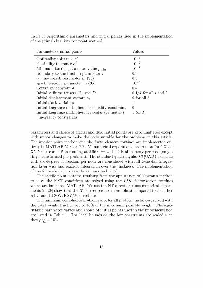
Table 1: Algorithmic parameters and initial points used in the implementationof the primal-dual interior point method.

Parameters/ initial points Values

Optimality tolerance εo 10−6

Feasibility tolerance εf 10−7

Minimum barrier parameter value µmin 10−8

Boundary to the fraction parameter τ 0.9η - line-search parameter in (35) 0.5τ0 - line-search parameter in (35) 10−5

Centrality constant σ 0.4Initial stiffness tensors Cil and Dil 0.1ρI for all i and lInitial displacement vectors u` 0 for all `Initial slack variables 1Initial Lagrange multipliers for equality constraints 0Initial Lagrange multipliers for scalar (or matrix) 1 (or I)

inequality constraints

parameters and choice of primal and dual initial points are kept unaltered exceptwith minor changes to make the code suitable for the problems in this article.The interior point method and the finite element routines are implemented en-tirely in MATLAB Version 7.7. All numerical experiments are run on Intel XeonX5650 six-core CPUs running at 2.66 GHz with 4GB of memory per core (only asingle core is used per problem). The standard quadrangular CQUAD4 elementswith six degrees of freedom per node are considered with full Gaussian integra-tion layer wise and explicit integration over the thickness. The implementationof the finite element is exactly as described in [9].

The saddle point systems resulting from the application of Newton’s methodto solve the KKT conditions are solved using the LDL factorization routineswhich are built into MATLAB. We use the NT direction since numerical experi-ments in [29] show that the NT directions are more robust compared to the otherAHO and HRVW/KSV/M directions.

The minimum compliance problems are, for all problem instances, solved withthe total weight fraction set to 40% of the maximum possible weight. The algo-rithmic parameter values and choice of initial points used in the implementationare listed in Table 1. The local bounds on the box constraints are scaled suchthat ρ/ρ = 105.

15

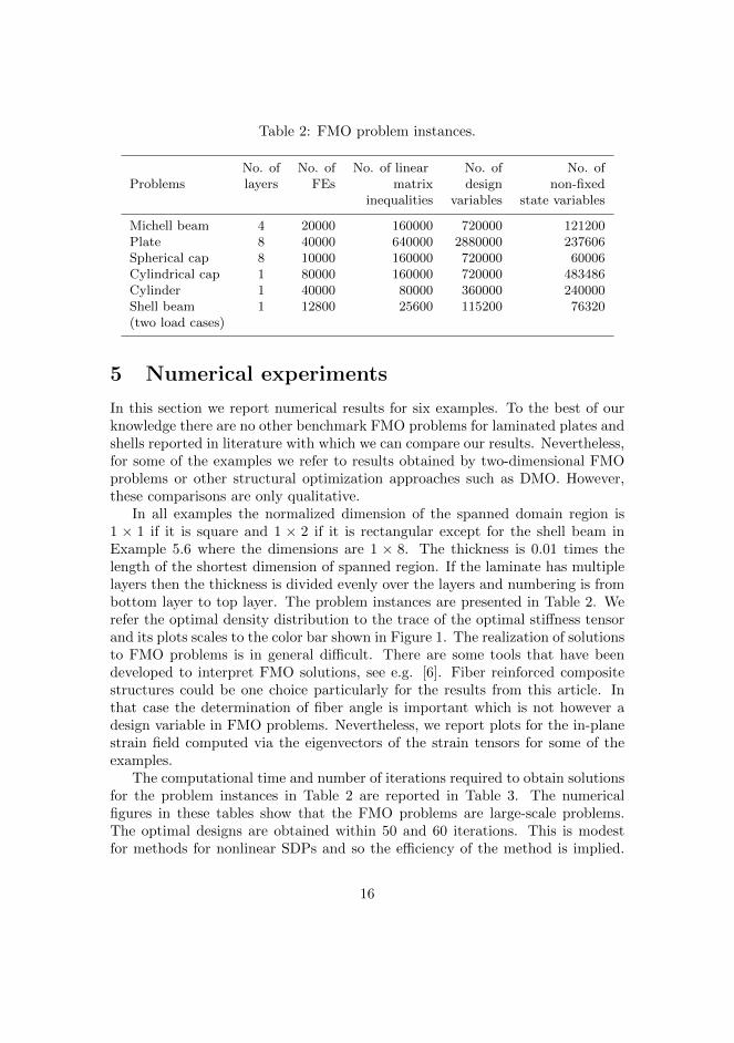
Table 2: FMO problem instances.

ProblemsNo. of No. of No. of linear No. of No. oflayers FEs matrix design non-fixed

inequalities variables state variables

Michell beam 4 20000 160000 720000 121200Plate 8 40000 640000 2880000 237606Spherical cap 8 10000 160000 720000 60006Cylindrical cap 1 80000 160000 720000 483486Cylinder 1 40000 80000 360000 240000Shell beam 1 12800 25600 115200 76320(two load cases)

5 Numerical experiments

In this section we report numerical results for six examples. To the best of ourknowledge there are no other benchmark FMO problems for laminated plates andshells reported in literature with which we can compare our results. Nevertheless,for some of the examples we refer to results obtained by two-dimensional FMOproblems or other structural optimization approaches such as DMO. However,these comparisons are only qualitative.

In all examples the normalized dimension of the spanned domain region is1 × 1 if it is square and 1 × 2 if it is rectangular except for the shell beam inExample 5.6 where the dimensions are 1 × 8. The thickness is 0.01 times thelength of the shortest dimension of spanned region. If the laminate has multiplelayers then the thickness is divided evenly over the layers and numbering is frombottom layer to top layer. The problem instances are presented in Table 2. Werefer the optimal density distribution to the trace of the optimal stiffness tensorand its plots scales to the color bar shown in Figure 1. The realization of solutionsto FMO problems is in general difficult. There are some tools that have beendeveloped to interpret FMO solutions, see e.g. [6]. Fiber reinforced compositestructures could be one choice particularly for the results from this article. Inthat case the determination of fiber angle is important which is not however adesign variable in FMO problems. Nevertheless, we report plots for the in-planestrain field computed via the eigenvectors of the strain tensors for some of theexamples.

The computational time and number of iterations required to obtain solutionsfor the problem instances in Table 2 are reported in Table 3. The numericalfigures in these tables show that the FMO problems are large-scale problems.The optimal designs are obtained within 50 and 60 iterations. This is modestfor methods for nonlinear SDPs and so the efficiency of the method is implied.

16

ρ ρ

Figure 1: Colorbar for the optimal density distribution.

(a) (b)

Figure 2: Design domain, boundary conditions, and external load (a), optimaldensity distribution (b) of the Michell beam consisting of four layers. The densitydistribution is identical in all layers as expected.

Studying the history of the iteration we also find that the direct solution of thesaddle point system dominates the computation time of the method. This is alsoillustrated in Table 3 where the computational time in solving multiple load FMOproblems dramatically increases.

Example 5.1. In the first example we consider a laminate of four plate layersclamped at one edge and subject to a pure in-plane load at the opposite edge asshown in Figure 2a. This example is included to show consistency of the models.The model gives results that are similar to solutions to two-dimensional FMOproblem in [33] and Variable Thickness Sheet problem in [8]. Figure 2b showsthat there is no distinction among the density distribution of the layers. Thenumerical values of the optimal solution also show that stiffness tensor C thataccounts for membrane deformation dominates the tensor D (which is zero overthe entire design domain). The traverse displacements are also zero. The in-planestrain field for the bottom layer is plotted in Figure 3. The other three layershave identical strain fields.

Example 5.2. In this example we consider a clamped laminate of eight platelayers subject to a uniformly distributed load, see Figure 4a. In the optimal

17

Figure 3: In-plane strain field of layer 1 for the Michell beam problem.

density distribution, shown in Figure 4b, the large interconnected reinforcementin the surface layers splits in to smaller edge and center reinforcements in thenext inner layers and then ends up in soft material in the innermost layers. Thisproperty resembles the expected sandwich structures. The in-plane strain fieldof the lower left corners of the bottom four layers is plotted in Figure 5. Thesestrain fields also correspond to that of the top four layers of equidistant from themidsurface. Therefore, the solution implies a symmetric laminate.

Example 5.3. We consider a hinged spherical cap of 8 layers subject to a singletransversal load concentrated at the center as shown in the Figure 6a. Thegeometry of the shell is adapted from [24]. The plot for the optimal distributionof materials is shown Figure 6b. There are wider stiff regions in the surfacelayers than the inner layers with the center reinforcement appearing in all layers.However, the symmetry behavior of the density distribution with respect to themidsurface does not exist. We can also find the correspondence of the solution toa sandwich structure and the unsymmetrical behavior in a solution to a similarDMO problem in [24].

Example 5.4. The design domain is a corner hinged cylindrical cap loaded bya transversal load concentrated at the center as shown in Figure 7a. The plotfor the optimal density distribution in Figure 7b shows the cross-like topologyextending from the center to the corners which can be found in other structuraloptimization approaches, see e.g., [16].

Example 5.5. In this example a cylinder is clamped at one end and is subjectto a load distributed on a small curve in the opposite end. All the nodal values of

18

(a)

(b)

Figure 4: Design domain, boundary conditions, and external load (a), optimaldensity distribution (b) of the clamped plate consisting of eight layers.

19

(a) (b)

(c) (d)

Figure 5: In-plane strain field of the bottom four layers of the lower left quartersfor the plate problem.

20

(a)

(b)

Figure 6: Design domain, boundary conditions, and external load (a), optimaldensity distribution (b) of the hinged spherical cap of eight layers.

21

(a) (b)

Figure 7: Design domain, boundary conditions, and external load (a), optimaldensity distribution (b) of the single layered cylindrical cap hinged at the fourcorners.

the load point in the same direction, see Figure 8a. The usual topology obtainedwhen solving a two-dimensional cantilever beam problem, see e.g., [29], can beseen in Figure 8b spanning from the loading curve to the fixed base on bothhalves of the cylinder.

Example 5.6. We consider a shell beam clamped at both ends subject to twoindependent loads distributed over lines lying at the middle of opposite lateralsurfaces as show in the Figure 9a. In the optimal design Figure 9b the stiffregions around the loading lines are extended and connected to the fixed regionsforming a chain of diamond-like topology over the top and bottom surfaces. Theresponse of the diamond like topology shows up in solutions to two-dimensionalFMO problem on a rectangular design domain clamped at its two opposite edgesand subject to two independent loads at the center of the other tow edges pointingin opposite directions, see [33]. Similar topology of the loaded surfaces can alsobe found in [31] while solving a single load problem over a three surface shellbeam.

6 Conclusions

We extended existing FMO models and a primal-dual interior point method forplates and shells to laminated structures for the first time. The consistency ofthe model is shown first by solving a well-known Michell beam problem under

22

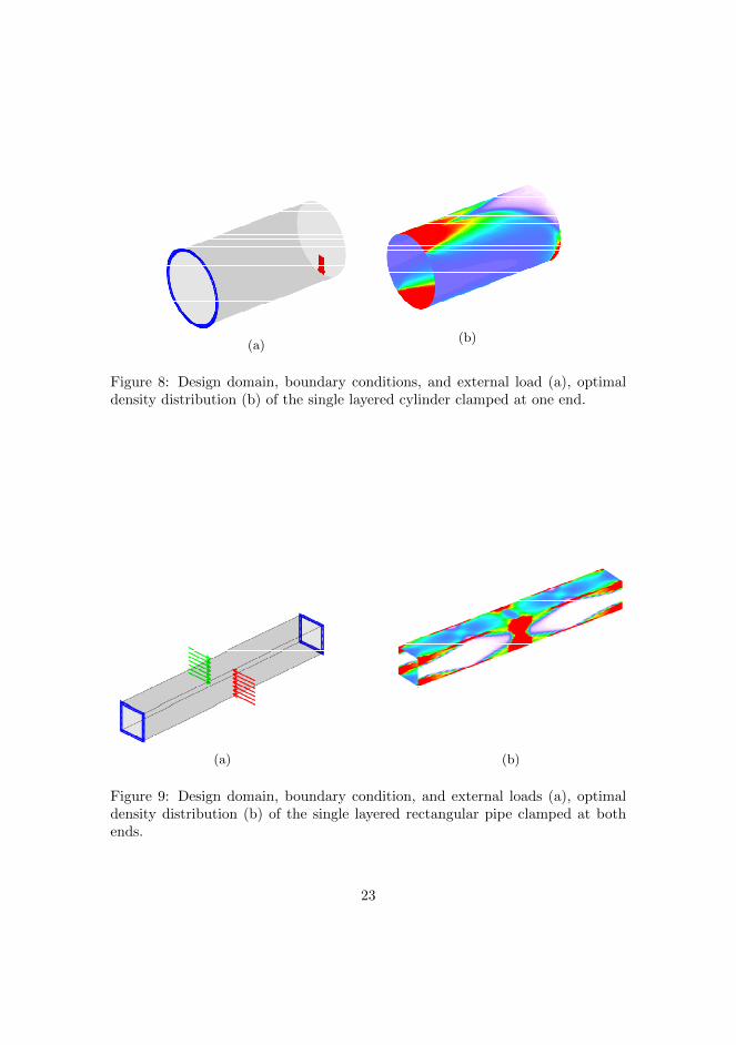
(a)(b)

Figure 8: Design domain, boundary conditions, and external load (a), optimaldensity distribution (b) of the single layered cylinder clamped at one end.

(a) (b)

Figure 9: Design domain, boundary condition, and external loads (a), optimaldensity distribution (b) of the single layered rectangular pipe clamped at bothends.

23

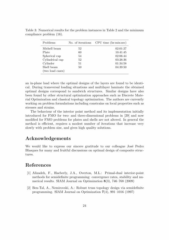
Table 3: Numerical results for the problem instances in Table 2 and the minimumcompliance problem (16).

Problems No. of iterations CPU time (hr:min:sec)

Michell beam 52 02:01:27Plate 60 10:41:45Spherical cap 54 02:06:44Cylindrical cap 52 03:26:36Cylinder 51 01:34:58Shell beam 50 04:39:50(two load cases)

an in-plane load where the optimal designs of the layers are found to be identi-cal. During transversal loading situations and multilayer laminate the obtainedoptimal designs correspond to sandwich structures. Similar designs have alsobeen found by other structural optimization approaches such as Discrete Mate-rial Optimization and classical topology optimization. The authors are currentlyworking on problem formulations including constrains on local properties such asstresses and strains.

The behaviour of the interior point method and its implementation initiallyintroduced for FMO for two- and three-dimensional problems in [29] and nowmodified for FMO problems for plates and shells are not altered. In general themethod is efficient, requires a modest number of iterations that increase veryslowly with problem size, and gives high quality solutions.

Acknowledgements

We would like to express our sincere gratitude to our colleague Jose PedroBlasques for many and fruitful discussions on optimal design of composite struc-tures.

References

[1] Alizadeh, F., Haeberly, J.A., Overton, M.L.: Primal-dual interior-pointmethods for semidefinite programming: convergence rates, stability and nu-merical results. SIAM Journal on Optimization 8(3), 746–768 (2009)

[2] Ben-Tal, A., Nemirovski, A.: Robust truss topology design via semidefiniteprogramming. SIAM Journal on Optimization 7(4), 991–1016 (1997)

24

[3] Bendsøe, M.P., Dıaz, A.R.: Optimization of material properties for Mindlinplate design. Structural Optimization 6, 268–270 (1993)

[4] Bendsøe, M.P., Guedes, J.M., Haber, R.B., Pedersen, P., Taylor, J.E.: Ananalytical model to predict optimal material properties in the context ofoptimal structural design. Journal of Applied Mechanics 61, 930–937 (1994)

[5] Blouza, A., Dret, H.L.: Nagdhi’s shell model: Existence, uniqueness andcontinuous dependence on the midsurface. Journal of elasticity 64, 199–216(2001)

[6] Bodnar, G., Stadelmeyer, P., Bogomolny, M.: Methods for computer aidedinterpretation of FMO results. Tech. rep., PLATO-N Public Report PU-R-3-2008 (2008). Available from http://www.plato-n.org/

[7] Chapelle, D., Bathe, K.J.: The Finite Element Analysis of Shells - Funda-mentals. Springer, Heidelberg (2003)

[8] Czarnecki, S., Lewinski, T.: On minimum compliance problems of thin elas-tic plates of varying thickness. Structural and Multidisciplinary Optimiza-tion 48(1), 17–31 (2013)

[9] Gaile, S.: Free material optimization for shells and plates. Ph.D. thesis, Insti-tute of Applied Mathematics II, Friedrich-Alexander University of Erlangen-Nuremberg (2011). Available from http://www.researchgate.net/

[10] Haslinger, J., Kocvara, M., Leugering, G., Stingl, M.: Multidisciplinary freematerial optimization. SIAM Journal on Applied Mathematics 70(7), 2709–2728 (2010)

[11] Helmberg, C., Rendl, F., Vanderbei, R.J., Wolkowicz, H.: An interior-pointmethod for semidefinite programming. SIAM Journal on Optimization 6,342–361 (1996)

[12] Kojima, M., Shindoh, S., Hara, S.: Interior-point methods for the monotonesemidefinite linear complementarity problem in symmetric matrices. SIAMJournal on Optimization 7(1), 86–125 (1997)

[13] Kocvara, M., Stingl, M.: A code for convex nonlinear and semidefinite pro-gramming. Optimization Methods and Software 18(3), 317–333 (2003)

[14] Kocvara, M., Stingl, M.: Free material optimization for stress constraints.Structural and Multidisciplinary Optimization 33, 323–355 (2007)

[15] Kocvara, M., Stingl, M., Zowe, J.: Free material optimization: recentprogress. Optimization 57(1), 79–100 (2008)

25

[16] Lee, S.J., Bae, J.E., Hinton, E.: Shell topology optimization using the lay-ered artificial material model. International Journal for Numerical Methodsin Engineering 47, 843–867 (2000)

[17] Lund, E., Stegmann, J.: On structural optimization of composite shell struc-tures using a discrete constitutive parametrization. Wind Energy 8, 109–124(2005)

[18] Monteiro, R.D.C.: Primal-dual path-following algorithms for semidefiniteprogramming. SIAM Journal on Optimization 7(3), 663–678 (1997)

[19] Nesterov, Y.E., Todd, M.J.: Self-scaled barriers and interior-point methodsfor convex programming. Mathematics of Operations Research 22(1), 1–42(1997)

[20] Nesterov, Y.E., Todd, M.J.: Primal-dual interior-point methods for self-scaled cones. SIAM Journal on Optimization 8(2), 324–364 (1998)

[21] Reddy, J.: Mechanics of laminated composite plates and shells: theory andanalysis, 2nd edn. London (2004)

[22] Ringertz, U.T.: On finding the optimal distribution of material properties.Structural Optimization 5, 265–267 (1993)

[23] Stegmann, J.: Analysis and optimization of laminated composite shell struc-tures. Ph.D. thesis, Institute of Mechanical Engineering, Aalborg University,Aalborg, Denmark (2004). Available from http://www.researchgate.net/

[24] Stegmann, J., Lund, E.: Discrete material optimization of general compositeshell structures. International Journal for Numerical Methods in Engineering62, 2009–2007 (2005)

[25] Stingl, M.: On the solution of nonlinear semidefinite programs by aug-mented lagrangian method. Ph.D. thesis, Institute of Applied MathematicsII, Friedrich-Alexander University of Erlangen-Nuremberg (2006). Availablefrom http://www2.am.uni-erlangen.de/

[26] Stingl, M., Kocvara, M., Leugering, G.: Free material optimization withfundamental eigenfrequency constraints. SIAM Journal on Optimization20(1), 524–547 (2009)

[27] Stingl, M., Kocvara, M., Leugering, G.: A new non-linear semidefinite pro-gramming algorithm with an application to multidisciplinary free materialoptimization. International Series of Numerical Mathematics 158, 275–295(2009)

26

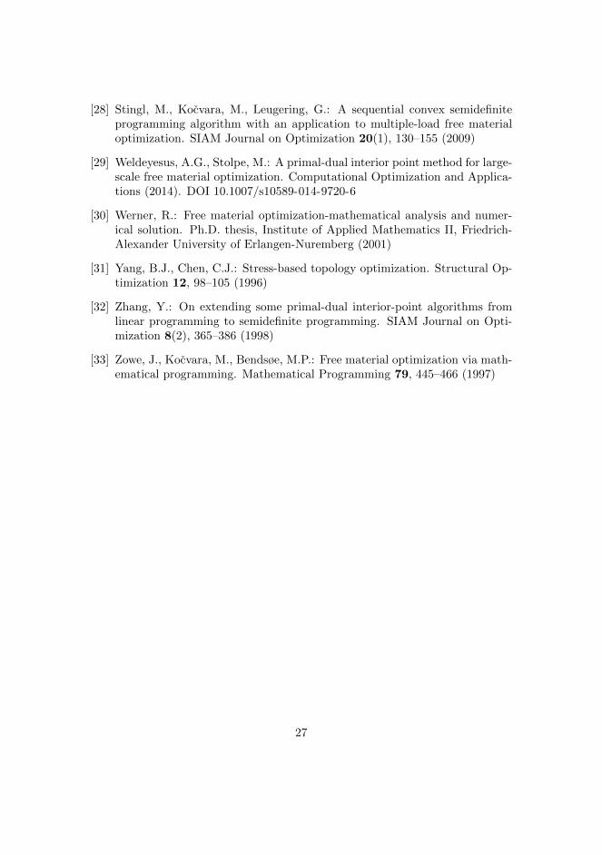
[28] Stingl, M., Kocvara, M., Leugering, G.: A sequential convex semidefiniteprogramming algorithm with an application to multiple-load free materialoptimization. SIAM Journal on Optimization 20(1), 130–155 (2009)

[29] Weldeyesus, A.G., Stolpe, M.: A primal-dual interior point method for large-scale free material optimization. Computational Optimization and Applica-tions (2014). DOI 10.1007/s10589-014-9720-6

[30] Werner, R.: Free material optimization-mathematical analysis and numer-ical solution. Ph.D. thesis, Institute of Applied Mathematics II, Friedrich-Alexander University of Erlangen-Nuremberg (2001)

[31] Yang, B.J., Chen, C.J.: Stress-based topology optimization. Structural Op-timization 12, 98–105 (1996)

[32] Zhang, Y.: On extending some primal-dual interior-point algorithms fromlinear programming to semidefinite programming. SIAM Journal on Opti-mization 8(2), 365–386 (1998)

[33] Zowe, J., Kocvara, M., Bendsøe, M.P.: Free material optimization via math-ematical programming. Mathematical Programming 79, 445–466 (1997)

27

Chapter 7

Models and methods forFree Material Optimizationwith local stress constraints

Weldeyesus, A.G.: Models and methods for Free Material Optimization withlocal stress constraints. Submitted to Journal of Structural and MultidisciplinaryOptimization in 2014. In review.

84

Models and Methods for Free Material

Optimization with Local Stress Constraints

Alemseged Gebrehiwot Weldeyesus∗

Abstract

Free Material Optimization (FMO) is a powerful approach of structuraloptimization of composite structures leading to conceptual optimal designs.The design variable is the elastic material tensor which is allowed to changeits values freely over the design domain giving optimal material propertiesand optimal material distribution. The only requirements are that the stiff-ness tensor is forced to be symmetric positive semidefinite as a necessarycondition for its physical attainability. One of the goals of this article tointroduce constraints on local stresses to existing FMO problems for lami-nated plates and shells and propose new stress constrained FMO problemformulations. The FMO problems are non convex semidefinite programwith a special structure involving many small matrix inequalities. Thisstructure is exploited by our special purpose optimization method. Thesecond goal of this article is to extend primal-dual interior point methodfor classical FMO problems to stress constrained FMO problems. Thenumerical experiments show that the optimal solutions to the stress con-strained problems can be achieved within a moderate number of iterations.The local stress constraints are satisfied with high accuracy. The methodand models are supported by numerical examples.

Mathematics Subject Classification 2010: 90C22, 90C90, 74P05, 74P15

Keywords: Structural optimization, free material optimization, nonlinear semidef-inite optimization, stress constraints

The research was partially funded by the Danish Council for Strategic Research throughthe Danish Center for Composite Structures and Materials (DCCSM).

∗DTU Wind Energy, Technical University of Denmark, Frederiksborgvej 399, 4000 Roskilde,Denmark. E-mail: alwel@dtu.dk

1

1 Introduction

Free Material Optimization (FMO) deals with obtaining a composite structurewith optimal material properties and optimal material distribution that can sus-tain a given set of loads. Such optimal structures can be considered as ultimatelybest structures among all possible elastic continua [36]. These optimal designscan also be used as benchmarks with which other designs obtained by otherapproaches of structural optimization can be compared.

The basic concept of FMO can be traced back to the early 1990s in [2], [3], and[22]. Since then there are several research studies dealing with more advancedFMO models. FMO formulations have been extended to include a wide range ofconstraints such as constraints on local stresses, local strains, displacement andfundamental frequencies in e.g. [17], [15], [11], and [25]. Theoretical aspects ofFMO problems including existence of optimal solutions are analyzed in differentstudies [11] and [34]. There are also numerical optimization methods proposedin several articles [36], [14], [24], [27], [26], and [33].

High stresses are one of the causes for engineering structures to fail. Thescope of several studies in structural optimization are extended to control stresseswithin a certain limit in the optimal structures. However, addressing stressesin the optimization problem is not straight forward. The choice of optimizationproblem formulation with relevant stress criteria and the development of methodsthat can computationally handle the problems are some of the main challenges.

Topology optimization is one of the research fields that has been extensivelystudied. For stress-based topology optimization see [35], [23], [5], [7], [20], and[18] for continua, and [13], [10], [29], and [30] for trusses and the referencestherein. Stresses are addressed in topology optimization in several ways. Oneway is limiting the stresses by introducing stress constraints which can be localat element level or global by aggregating the stresses in the design. Addingsuch constraints however leads to optimization problems that are difficult tosolve. Suitable mathematical properties such as convexity are lost. Moreover,the problems face the singularity phenomenon described in e.g. [13] and [1]among many others.

FMO problems with stress constraints are analyzed and solved in [17], [16],and [15] for two-dimensional and in [11] for three-dimensional structures. Theconstraints are introduced with a term of an integral of the norm of the stresses.One of the outcome of FMO models is that higher stresses are primarily removedby changing material properties. This is unlike to other approaches in structuraloptimization where the materials are fixed and higher stresses are avoided byother ways, for e.g., changing the geometry of the optimal structure. The resultis supported by making a comparison between solutions to FMO problem andthe classical Variable Thickness Sheet (VTS) problem in [15].

2

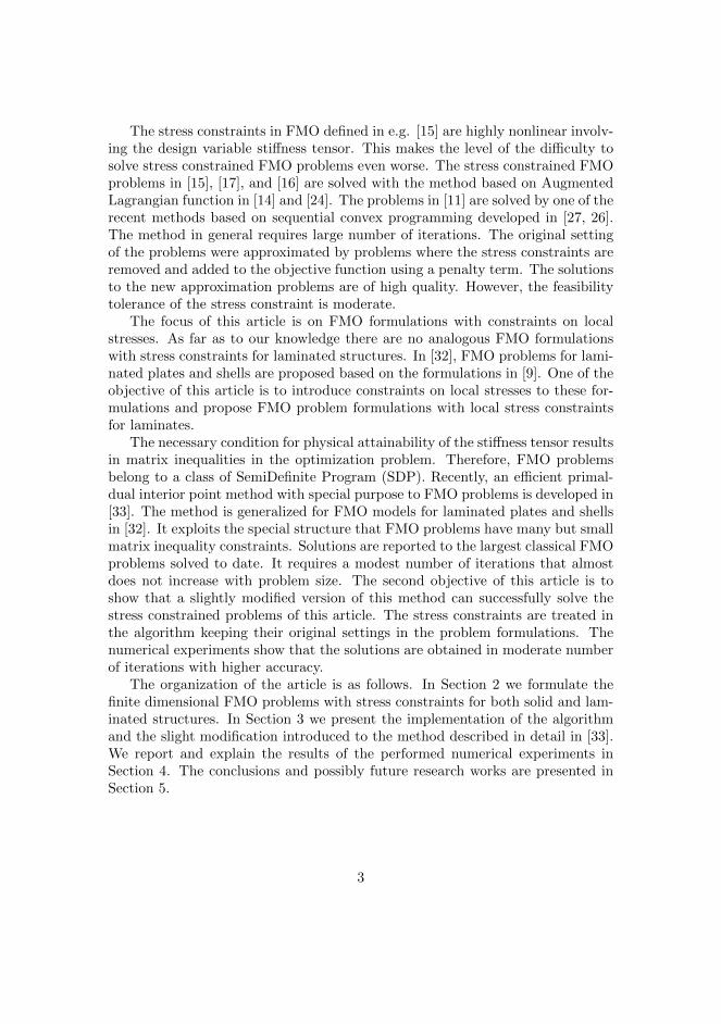
The stress constraints in FMO defined in e.g. [15] are highly nonlinear involv-ing the design variable stiffness tensor. This makes the level of the difficulty tosolve stress constrained FMO problems even worse. The stress constrained FMOproblems in [15], [17], and [16] are solved with the method based on AugmentedLagrangian function in [14] and [24]. The problems in [11] are solved by one of therecent methods based on sequential convex programming developed in [27, 26].The method in general requires large number of iterations. The original settingof the problems were approximated by problems where the stress constraints areremoved and added to the objective function using a penalty term. The solutionsto the new approximation problems are of high quality. However, the feasibilitytolerance of the stress constraint is moderate.

The focus of this article is on FMO formulations with constraints on localstresses. As far as to our knowledge there are no analogous FMO formulationswith stress constraints for laminated structures. In [32], FMO problems for lami-nated plates and shells are proposed based on the formulations in [9]. One of theobjective of this article is to introduce constraints on local stresses to these for-mulations and propose FMO problem formulations with local stress constraintsfor laminates.

The necessary condition for physical attainability of the stiffness tensor resultsin matrix inequalities in the optimization problem. Therefore, FMO problemsbelong to a class of SemiDefinite Program (SDP). Recently, an efficient primal-dual interior point method with special purpose to FMO problems is developed in[33]. The method is generalized for FMO models for laminated plates and shellsin [32]. It exploits the special structure that FMO problems have many but smallmatrix inequality constraints. Solutions are reported to the largest classical FMOproblems solved to date. It requires a modest number of iterations that almostdoes not increase with problem size. The second objective of this article is toshow that a slightly modified version of this method can successfully solve thestress constrained problems of this article. The stress constraints are treated inthe algorithm keeping their original settings in the problem formulations. Thenumerical experiments show that the solutions are obtained in moderate numberof iterations with higher accuracy.

The organization of the article is as follows. In Section 2 we formulate thefinite dimensional FMO problems with stress constraints for both solid and lam-inated structures. In Section 3 we present the implementation of the algorithmand the slight modification introduced to the method described in detail in [33].We report and explain the results of the performed numerical experiments inSection 4. The conclusions and possibly future research works are presented inSection 5.

3

2 Problem formulations

In this section we present FMO problem formulations with stress constraints forsolid and laminated plate and shell structures. In both cases we start with thediscrete version of the classical minimum compliance (maximum stiffness) and theminimum weight FMO formulations. For details on the problem formulations andfinite element discretization, see [27] and [17] for solid structures, and [32], [9],and [4] for laminated structures.

It is pointed out in e.g. [15] that addressing stress constraints in structuraloptimization using FMO is a challenge. In the first place, there is no existing gen-eral failure criterion. The realization of the optimal structure is also importantin using one of the several existing failure criteria, for example see [12] for dif-ferent failure criteria in fiber reinforced composites. Moreover, in FMO materialproperties are also design variables giving conceptual optimal designs. Despitethese challenges we follow the measure proposed in [15] which is the norm of thestresses integrated over the finite element in the discrete problems.

In FMO problem formulations the requirement of the physical attainability ofthe stiffness tensor is introduced by matrix inequality constraints. As a measureof stiffness the trace of the elastic stiffness tensor is used. It is locally boundedfrom above by ρ to avoid arbitrarily stiff materials and from below by ρ to limitthe extent of softness. These bounds must satisfy the relation 0 ≤ ρ < ρ < ∞.We consider nL given external static nodal load vectors f` ∈ Rn, where ` ∈L = 1, . . . , nL and n is the number of finite element degrees of freedom. Weprescribe weights w` for the loads f` satisfying

∑` w` = 1 and w` > 0 for each

` ∈ L.Next, we present the FMO problems with local constraints for solids and lam-

inated structures. In both cases we follow similar approach. We first formulatethe problems without stress constraints. Then, we define the stress constraintsand include in the unconstrained problems to formulate the stress constrainedFMO problems.

2.1 FMO for solid structures

This section is essentially identical to the corresponding section in [33] and isincluded for completeness. We consider a design domain Ω partitioned in to muniform finite elements Ωi for i = 1, . . . ,m. The elastic stiffness tensor E(x)is approximated by a function that is constant on each finite element with itselement values making the vector of block matrices E = (E1, . . . , Em)T . For anygiven external static nodal load vectors f`, the associated displacement u` mustsatisfy the linear elastic equilibrium equation

A(E)u` = f`, ` ∈ L, (1)

4

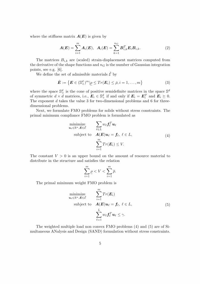
where the stiffness matrix A(E) is given by

A(E) =m∑

i=1

Ai(E), Ai(E) =

nG∑

k=1

BTi,kEiBi,k. (2)

The matrices Bi,k are (scaled) strain-displacement matrices computed fromthe derivative of the shape functions and nG is the number of Gaussian integrationpoints, see e.g. [6].

We define the set of admissible materials E by

E :=E ∈ (Sd+)m|ρ ≤ Tr(Ei) ≤ ρ, i = 1, . . . ,m

(3)

where the space Sd+ is the cone of positive semidefinite matrices in the space Sdof symmetric d × d matrices, i.e., Ei ∈ Sd+ if and only if Ei = ET

i and Ei 0.The exponent d takes the value 3 for two-dimensional problems and 6 for three-dimensional problems.

Next, we formulate FMO problems for solids without stress constraints. Theprimal minimum compliance FMO problem is formulated as

minimizeu`∈Rn,E∈E

∑

`∈Lw`f

T` u`

subject to A(E)u` = f`, ` ∈ L,m∑

i=1

Tr(Ei) ≤ V.

(4)

The constant V > 0 is an upper bound on the amount of resource material todistribute in the structure and satisfies the relation

m∑

i=1

ρ < V <m∑

i=1

ρ.

The primal minimum weight FMO problem is

minimizeu`∈Rn,E∈E

m∑

i=1

Tr(Ei)

subject to A(E)u` = f`, ` ∈ L,L∑

`=1

w`fT` u` ≤ γ.

(5)

The weighted multiple load non convex FMO problems (4) and (5) are of Si-multaneous ANalysis and Design (SAND) formulation without stress constraints.

5

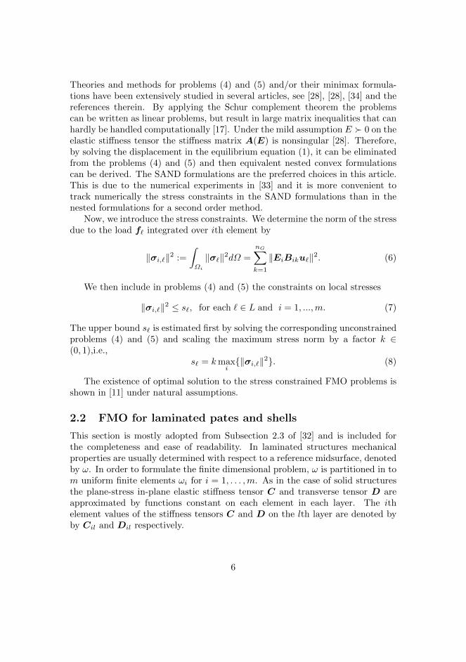
Theories and methods for problems (4) and (5) and/or their minimax formula-tions have been extensively studied in several articles, see [28], [28], [34] and thereferences therein. By applying the Schur complement theorem the problemscan be written as linear problems, but result in large matrix inequalities that canhardly be handled computationally [17]. Under the mild assumption E 0 on theelastic stiffness tensor the stiffness matrix A(E) is nonsingular [28]. Therefore,by solving the displacement in the equilibrium equation (1), it can be eliminatedfrom the problems (4) and (5) and then equivalent nested convex formulationscan be derived. The SAND formulations are the preferred choices in this article.This is due to the numerical experiments in [33] and it is more convenient totrack numerically the stress constraints in the SAND formulations than in thenested formulations for a second order method.

Now, we introduce the stress constraints. We determine the norm of the stressdue to the load f` integrated over ith element by

‖σi,`‖2 :=

∫

Ωi

‖σ`‖2dΩ =

nG∑

k=1

‖EiBiku`‖2. (6)

We then include in problems (4) and (5) the constraints on local stresses

‖σi,`‖2 ≤ s`, for each ` ∈ L and i = 1, ...,m. (7)

The upper bound s` is estimated first by solving the corresponding unconstrainedproblems (4) and (5) and scaling the maximum stress norm by a factor k ∈(0, 1),i.e.,

s` = kmaxi‖σi,`‖2. (8)

The existence of optimal solution to the stress constrained FMO problems isshown in [11] under natural assumptions.

2.2 FMO for laminated pates and shells

This section is mostly adopted from Subsection 2.3 of [32] and is included forthe completeness and ease of readability. In laminated structures mechanicalproperties are usually determined with respect to a reference midsurface, denotedby ω. In order to formulate the finite dimensional problem, ω is partitioned in tom uniform finite elements ωi for i = 1, . . . ,m. As in the case of solid structuresthe plane-stress in-plane elastic stiffness tensor C and transverse tensor D areapproximated by functions constant on each element in each layer. The ithelement values of the stiffness tensors C and D on the lth layer are denoted byby Cil and Dil respectively.

6

Given external static nodal load vectors f` the resulting displacement (u,θ)`(translational and rotational) satisfies the elastic equilibrium equation

K(C,D)(u,θ)` = f`, ` ∈ L, (9)

where K(C,D) the stiffness matrix is given by

K(C,D) =

m∑

i=1

(Kγi (C) +Kγχ

i (C) + (Kγχi (C))T +Kχ

i (C) +Kζi (D)). (10)

The element stiffness matrices in (10) are given by

Kγi (C) =

∑

l,(j,k)∈ni

∫

ωi

til(Bγjl)

TCilBγkldS (11a)

Kγχi (C) =

∑

l,(j,k)∈ni

∫

ωi

til(Bγjl)

TCilBχkldS (11b)

Kχi (C) =

N∑

l,(j,k)∈ni

∫

ωi

˜til(Bχjl)

TCilBχkldS (11c)

Kζi (D) = κ

∑

l,(j,k)∈ni

∫

ωi

til(Bζjl)

TDilBζkldS, (11d)

where ni is the index set of nodes associated with the element ωi. The matricesBγil, B

γil and Bζi,l are the (scaled) strain-displacement matrices for membrane

strains, for bending strains, and for shear strains, respectively. The factors til,

til and ˜til are computed as

til = tbil − tail, til =1

2((tbil)

2 − (tail)2),

˜til =1

3((tbil)

3 − (tail)3), (12)

where tbil and tail the upper and lower transverse coordinates of the lth layer atthe center of the element ωi. The coefficient κ < 1 appearing in the shear term in(11d) is the shear correction factor. This is to take into account the shell modelwhich is used in applications.

Given that the laminate has N number of layers we define the set of admissible

7

material E by

E =

(C,D) ∈ (S3+)mN × (S2+)mN

∣∣∣∣

ρ ≤ til(Tr(Cil) + 1

2Tr(Dil))≤ ρ, i = 1, . . . ,m, l = 1, . . . , N

. (13)

Now, we formulate the unconstrained problems. The primal minimum com-pliance FMO formulation is then stated as

minimize(u,θ)`∈Rn,(C,D)∈E

∑

`∈Lw`(f`)

T (u,θ)`

subject to K(C,D)(u,θ)` = f`, ` ∈ L,m∑

i=1

N∑

l=1

til

(Tr(Cil) +

1

2Tr(Dil)

)≤ V,

(14)

with the volume bound V > 0 satisfying

N∑

l=1

m∑

i=1

ρ < V <N∑

l=1

m∑

i=1

ρ.

The discrete primal minimum weight FMO formulation is

minimize(u,θ)`∈Rn,(C,D)∈E

m∑

i=1

N∑

l=1

til

(Tr(Cil) +

1

2Tr(Dil)

)

subject to K(C,D)(u,θ)` = f`, ` ∈ L,∑

`∈Lw`(f`)

T (u,θ)` ≤ γ.

(15)

Next, we present our motivation for the type of stress constraints that we intro-duce to the problems (14) and (15).

It is known from mechanics of laminated structures that stresses vary acrossthe thickness of the laminate with linear variation within a layer (we are talkingabout linear elasticity). Therefore, we make two stress evaluations in each layerover each element ωi, at the top and lower transverse coordinates of the layer.This allows us to capture the stress extremities within each layer and each ele-ment. We follow similar approach proposed for solids and make these evaluationsby the integral form of stresses, i.e., analogous to (6). The stress due to the load

8

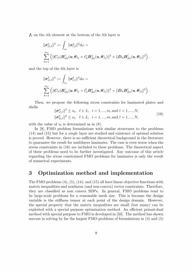
f` on the ith element at the bottom of the lth layer is

‖σail,`‖2 :=

∫

ωi

‖σal,`‖2dω =

nG∑

k=1

(‖Cil(Bγ

ikl(u,θ)` + tailBχikl(u,θ)`)‖2 + ‖DilB

ζikl(u,θ)`‖2

).

and the top of the lth layer is

‖σbil,`‖2 :=

∫

ωi

‖σbl,`‖2dω =

nG∑

k=1

(‖Cil(Bγ

ikl(u,θ)` + tbilBχikl(u,θ)`)‖2 + ‖DilB

ζikl(u,θ)`‖2

).

Then, we propose the following stress constraints for laminated plates andshells

‖σail,`‖2 ≤ s`, ` ∈ L, i = 1, ...,m, and l = 1, ..., N,

‖σbil,`‖2 ≤ s`, ` ∈ L, i = 1, ...,m, and l = 1, ..., N,(16)

with the value of s` is determined as in (8).In [9], FMO problem formulations with similar structures to the problems

(14) and (15) but for a single layer are studied and existence of optimal solutionis proved. However, there is no sufficient theoretical background in the literatureto guarantee the result for multilayer laminates. The case is even worse when thestress constraints in (16) are included to these problems. The theoretical aspectof these problems need to be further investigated. Any outcome of this articleregarding the stress constrained FMO problems for laminates is only the resultof numerical experiments.

3 Optimization method and implementation

The FMO problems (4), (5), (14), and (15) all have linear objective functions withmatrix inequalities and nonlinear (and non convex) vector constraints. Therefore,they are classified as non convex SDPs. In general, FMO problems tend tobe large-scale problems for a reasonable mesh size. This is because the designvariable is the stiffness tensor at each point of the design domain. However,the special property that the matrix inequalities are small (but many) can beexploited with a special purpose optimization method. An efficient primal-dualmethod with special purpose to FMO is developed in [33]. The method has shownsuccess in solving by far the largest FMO problems of formulations in (4) and (5)

9

and some other equivalent formulations. It is also generalized in [32] to solve theFMO problems for laminates of the formulation in (14).

Stress constrained structural optimization problems are in general difficultproblems to solve and usually computationally expensive. The problems maynot also satisfy constraint qualifications [1], stated as singularity phenomenonin [13]. The stress constraints for FMO problems in (7) and (16) are highlynonlinear in the stiffness tensor and displacement. Hence, the challenge in thehandling of computations and finding accurate solutions rises to a complex issuein FMO problems with stress constraints.

In this article we slightly modify the primal-dual interior point method de-veloped in [33] and [32] to solve the stress constrained problems. We employ aperturbation to the the coefficient matrix of the saddle point system that resultsduring applying Newton’s method to solve the optimality conditions. This isbased on inertia controlling methods [19, 8, 31] to ensures that a search directiongives a decrease in the merit function chosen in the algorithm.

The stress constraints are treated in the algorithm directly keeping their orig-inal settings in (7) and (16). In other studies these are often moved to the ob-jective function using a penalty term [27, 26]. The code is entirely implementedin MATLAB. The standard QUAD4 bilinear elements obtained by full Gaussianintegration are considered for the two-dimensional problems. For the laminateproblems we consider the standard quadrangular CQUAD4 elements with sixdegrees of freedom per node with full Gaussian integration layer wise and ex-plicit integration over the thickness. The overview of algorithmic parameters aredescribed in [33] and [32].

4 Numerical experiments

For the numerical experiments we consider the minimum compliance problems(4) together with stress constraints (7) for two-dimensional problems, and (14)together with the stress constraints (16) for problems on laminated structures.The total weight fraction is set to 40% of the maximum possible weight and thebounds on the traces of the stiffness tensors are scaled such that ρ/ρ = 105.

Through out this section we use the color scale with limits ρ and ρ given inFigure 1 for all plots of the optimal density distribution. We use own color scalesfor plots of optimal stress norms to easily show high stresses in the unconstrainedproblems and regions of active stress constraints in the constrained problems.Note that the labels of the color bar are the norm of the stresses, not the normof the stresses squared, as used in Table 3. For the two-dimensional Examples4.1 and 4.2 we also report the principal stress directions which are computed asprincipal eigenvectors associated to the Voigt-stress tensor.

10

ρ ρ

Figure 1: Color bar for the plots of optimal density distribution.

There are five examples in this section. The first two examples are for two-dimensional problems and the last three examples are for laminated structures.In Example 4.1 we consider L-shaped design domain of dimension (normalized)1×1 and a quarter removed from one of the corners. In Example 4.2 we considera Michell beam problem on a rectangular design domain of dimension 2× 1. Forthe examples on laminates we consider a laminate spanning a region of dimension1×1 for the clamped plates in Examples 4.3 and 4.4, and 1×8 for the shell beamin Example 4.5. The ratio of the thickness to the shortest dimension is 0.01 andis distributed evenly for layered laminates. Layers are numbered in the thicknessdirection from bottom to top. The problem instances are presented in Tables 1and 2.

The numerical results are reported in Table 3 listing some comparisons be-tween solving the constrained and unconstrained problems. The optimality tol-erances are the norm of the fist-order optimality conditions measured withoutperturbation on the complementarity conditions. By feasibility tolerances wealso refer ot the feasibility of the stress constraints in the original problem set-tings (7) and (16). Looking at the numerical values the active stress constraintsare feasible with high accuracy. The solutions to the unconstrained problemsare obtained within 30 and 61 iterations where as within 85 and 142 for theconstrained problems. This can be considered as modest taking in to accountthat the problems are nonlinear SDPs. Moreover, the number of iterations ismodest compared to the results in other literatures, see for example [16] for twodimensional, and [11] for three-dimensional problems. The increase in the num-ber of iterations in solving the constrained problems is expected since the stressconstraints are nonlinear involving matrix variables. It is common practice instructural optimization that stresses are reduced at the cost of an increase incompliance. This is also shown in Table 3 for FMO problems. However, thesurprising outcome from the numerical experiments is that compliances are wors-ened not significantly in FMO. In all examples the increase in compliance is lessthan 5% while stresses are reduced by more than 50%

In all cases, higher stresses near the fixed or loaded regions in the uncon-strained problems are avoided in the constrained problems. For a physicallymeaningful chosen values of the scaling factor k in (8), the stress constraints arefound to be active in wider stiff regions of the optimal designs in the constrained

11

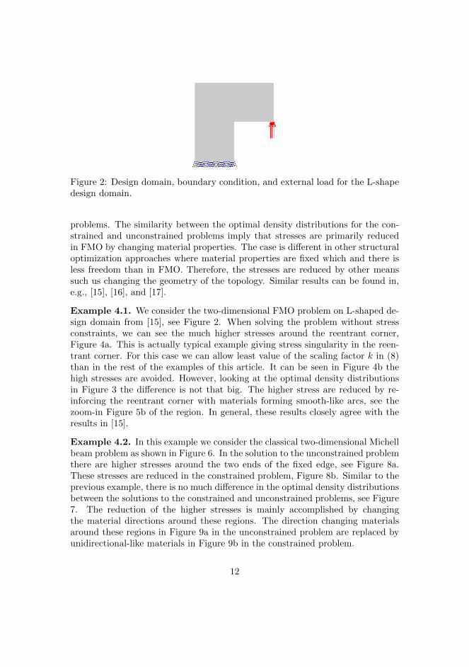
Figure 2: Design domain, boundary condition, and external load for the L-shapedesign domain.

problems. The similarity between the optimal density distributions for the con-strained and unconstrained problems imply that stresses are primarily reducedin FMO by changing material properties. The case is different in other structuraloptimization approaches where material properties are fixed which and there isless freedom than in FMO. Therefore, the stresses are reduced by other meanssuch us changing the geometry of the topology. Similar results can be found in,e.g., [15], [16], and [17].

Example 4.1. We consider the two-dimensional FMO problem on L-shaped de-sign domain from [15], see Figure 2. When solving the problem without stressconstraints, we can see the much higher stresses around the reentrant corner,Figure 4a. This is actually typical example giving stress singularity in the reen-trant corner. For this case we can allow least value of the scaling factor k in (8)than in the rest of the examples of this article. It can be seen in Figure 4b thehigh stresses are avoided. However, looking at the optimal density distributionsin Figure 3 the difference is not that big. The higher stress are reduced by re-inforcing the reentrant corner with materials forming smooth-like arcs, see thezoom-in Figure 5b of the region. In general, these results closely agree with theresults in [15].

Example 4.2. In this example we consider the classical two-dimensional Michellbeam problem as shown in Figure 6. In the solution to the unconstrained problemthere are higher stresses around the two ends of the fixed edge, see Figure 8a.These stresses are reduced in the constrained problem, Figure 8b. Similar to theprevious example, there is no much difference in the optimal density distributionsbetween the solutions to the constrained and unconstrained problems, see Figure7. The reduction of the higher stresses is mainly accomplished by changingthe material directions around these regions. The direction changing materialsaround these regions in Figure 9a in the unconstrained problem are replaced byunidirectional-like materials in Figure 9b in the constrained problem.

12

Tab

le1:

FM

Opro

ble

min

stan

ces

for

the

two-d

imen

sional

pro

ble

ms.

Pro

ble

ms

No.

of

FE

sN

o.

stre

ssN

o.

of

lin

ear

matr

ixN

o.

of

des

ign

No.

of

non

-fixed

con

stra

ints

ineq

uali

ties

vari

ab

les

state

vari

ab

les

L-s

hap

e7500

7500

7500

45000

15300

Mic

hel

lb

eam

20000

20000

20000

120000

40400

Tab

le2:

FM

Opro

ble

min

stan

ces

for

the

lam

inate

pro

ble

ms.

Pro

ble

ms

No.

of

layer

sN

o.

of

FE

sN

o.

stre

ssN

o.

of

lin

ear

matr

ixN

o.

of

des

ign

No.

of

non

-fixed

con

stra

ints

ineq

uali

ties

vari

ab

les

state

vari

ab

les

Cla

mp

edp

late

(pre

ssure

load

)8

2500

40000

40000

180000

14406

Cla

mp

edp

late

(cen

tral

load

)8

2500

40000

40000

180000

14406

Sh

ell

bea

m(t

wo

load

case

s)1

12800

51200

25600

115200

76320

Tab

le3:

Num

eric

alre

sult

sfo

rth

epro

ble

min

stan

ces

inT

able

s1

and

2and

the

min

imum

com

pliance

pro

ble

ms

(4)

and

(14)

wit

hth

est

ress

const

rain

ts(7

)an

d(1

6)re

spec

tive

ly.

(Com

pliance

and

stre

ssnorm

sare

scale

d)

Pro

ble

ms

Wit

hou

tst

ress

con

stra

ints

Wit

hst

ress

con

stra

ints

Iter

Com

pl-

Max.

tres

sO

pt/

feas

kIt

erC

om

pl-

Max.

stre

ssO

pt/

feas

ian

cen

orm

tole

ran

ces

ian

cen

orm

tole

ran

ces

L-s

hap

e30

1.8

951

1.3

206

2.7

e-08/4.0

e-10

0.2

85

1.9

281

0.2

643

9.5

e-08/8.9

e-09

Mic

hel

lB

eam

47

2.4

427

1.9

372

8.1

e-08/1.7

e-11

0.4

102

2.4

579

0.7

749

8.5

e-08/4.3

e-10

Cla

mp

edp

late

(pre

ssure

load

)47

5.4

771

2.1

574

3.4

e-07/6.9

e-09

0.5

115

5.5

624

1.0

783

6.5

e-06/8.8

e-07

Cla

mp

edp

late

(cen

tral

load

)54

7.1

531

9.3

224

3.5

e-07/3.0

e-08

0.5

138

7.1

876

4.6

612

3.7

e-07/9.6

e-09

Sh

ell

bea

m(t

wo

load

case

s)61

6.5

645

0.1

370

7.6

e-07/5.9

e-09

0.4

142

6.7

257

0.0

548

3.4

e-07/7.9

e-10

13

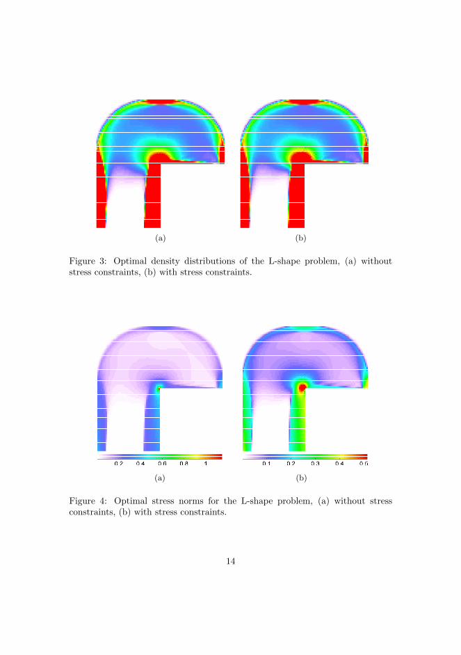
(a) (b)

Figure 3: Optimal density distributions of the L-shape problem, (a) withoutstress constraints, (b) with stress constraints.

(a) (b)

Figure 4: Optimal stress norms for the L-shape problem, (a) without stressconstraints, (b) with stress constraints.

14

0.2 0.4 0.6 0.8 1

(a)

0.1 0.2 0.3 0.4 0.5

(b)

Figure 5: Optimal principal stresses around the reentrant corner for the L-shapeproblem, (a) without stress constraints, (b) with stress constraints.

Figure 6: Design domain, boundary condition, and external load for the Michellbeam problem.

(a) (b)

Figure 7: Optimal density distributions for the Michell beam problem, (a) with-out stress constraints, (b) with stress constraints.

15

(a) (b)

Figure 8: Optimal stress norms for the Michell beam problem, (a) without stressconstraints, (b) with stress constraints.

0.2 0.4 0.6 0.8 1 1.2

(a)

0.2 0.4 0.6 0.8

(b)

Figure 9: Optimal principal stresses around the upper left corner for the Michellbeam problem, (a) without stress constraints, (b) with stress constraints.

16

Figure 10: Design domain, boundary condition, and external load for the clampedplate with pressure load.

Example 4.3. We consider a clamped plate of eight layers loaded uniformly,see Figure 10. In this case the optimal solution corresponds to a sandwich-like symmetric laminate. Therefore, we report results only for the bottom fourlayers. Looking at the density distributions in Figure 11, we notice a slightvisible difference in the middle four layers where some more materials are usedaround the fixed regions in the constrained problem than in the unconstrainedproblem. Figure 12 shows that there are higher stresses in the surface layersmainly concentrated around the fixed four edges of the plate. These are controlledto be within the limit in the constrained problem, Figure 13.

In our model we follow the First Order Deformation Theory (FSDT), see[21], in which the out-of-plane shear stresses are taken in to account. Unlikethe two-dimensional problems, reporting the mechanism by which high stressare avoided is not straight forward for laminates. Hence, the realization of thesolutions to FMO problems for laminates needs further investigation. This appliesto examples 4.3, 4.4 and 4.5 of this article.

Example 4.4. We consider a similar case as example 4.3, a clamped laminateof eight plate layers but with the load concentrated at the center, see Figure 14.This is to consider a situation where local higher stresses are located around theloaded area. The solution again gives a sandwich-like symmetric laminate withthe stiff area around the center appearing in all layers. The plots are for the firstfour layers. In the unconstrained problem we can see from Figure 16 that thereare higher stresses in a small region around the center and mainly in the surfacelayers. These are avoided in the constrained problem 17 and all layers around

17

(a)

(b)

Figure 11: Optimal density distributions of the first four layers for the clampedplate with pressure load, (a) without stress constraints, (b) with stress con-straints.

18

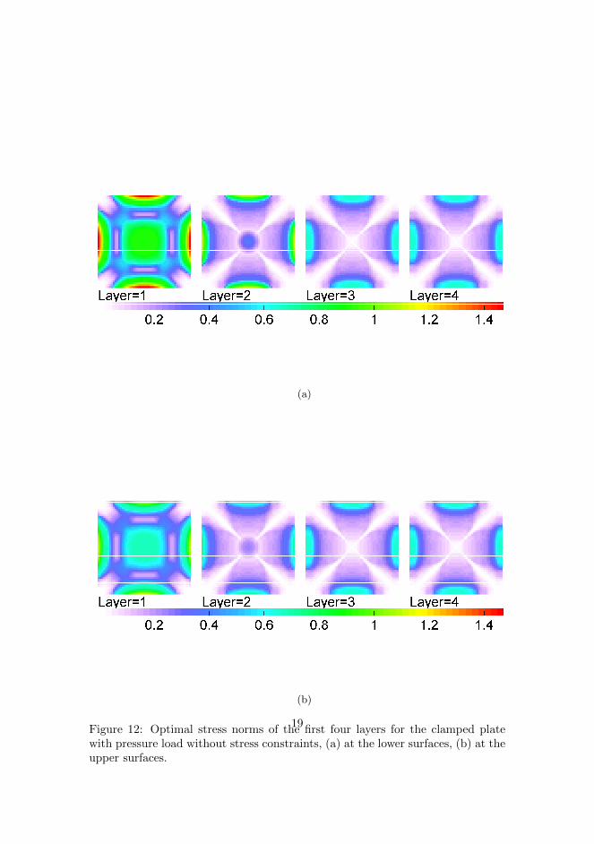
(a)

(b)

Figure 12: Optimal stress norms of the first four layers for the clamped platewith pressure load without stress constraints, (a) at the lower surfaces, (b) at theupper surfaces.

19

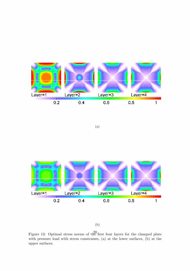
(a)

(b)

Figure 13: Optimal stress norms of the first four layers for the clamped platewith pressure load with stress constraints, (a) at the lower surfaces, (b) at theupper surfaces.

20

Figure 14: Design domain, boundary condition, and external load for the clampedplate with a point load at the center.

this region are involved in carrying the reduced stress. The density distributionsare more or less similar, Figure 15.

Example 4.5. In this example we solve a two load case problem on a shell beamclamped at both ends loaded as in Figure 18. We report the plots for the optimalstress norms of the outer surface for one of the loads. The other cases can easilybe determined from these plots. The higher stresses around the loaded regionshown in Figure 20a in the unconstrained problem are avoided in the constrainedproblem, see Figure 20b. There is no clear difference in the topology of theoptimal density distributions, Figure 19.

5 Conclusions

We introduce stress constraints to the FMO models proposed by the authors in[32] for laminated plates and shells for the first time. We extend the efficientprimal-dual interior point method initially developed in [33] for solids and lattergeneralized in [32] for laminates to solve these stress constrained FMO problems.In the numerical experiments the high stresses in the unconstrained problemswhich occur mostly near the fixed or loaded areas are reduced in the constrainedproblems. The feasibility of the stress constraints is higher than we find in otherarticles (literatures are available only for solids). The number of iterations re-quired to obtain solution to the problems of this article is between 85 and 142.This is modest considering the highly nonlinearity of the stress constraints andnon-convexity of the problems. The efficiency of the method is implied indeed.

21

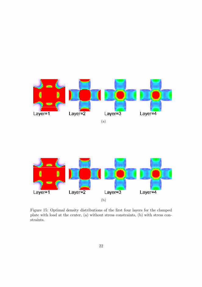
(a)

(b)

Figure 15: Optimal density distributions of the first four layers for the clampedplate with load at the center, (a) without stress constraints, (b) with stress con-straints.

22

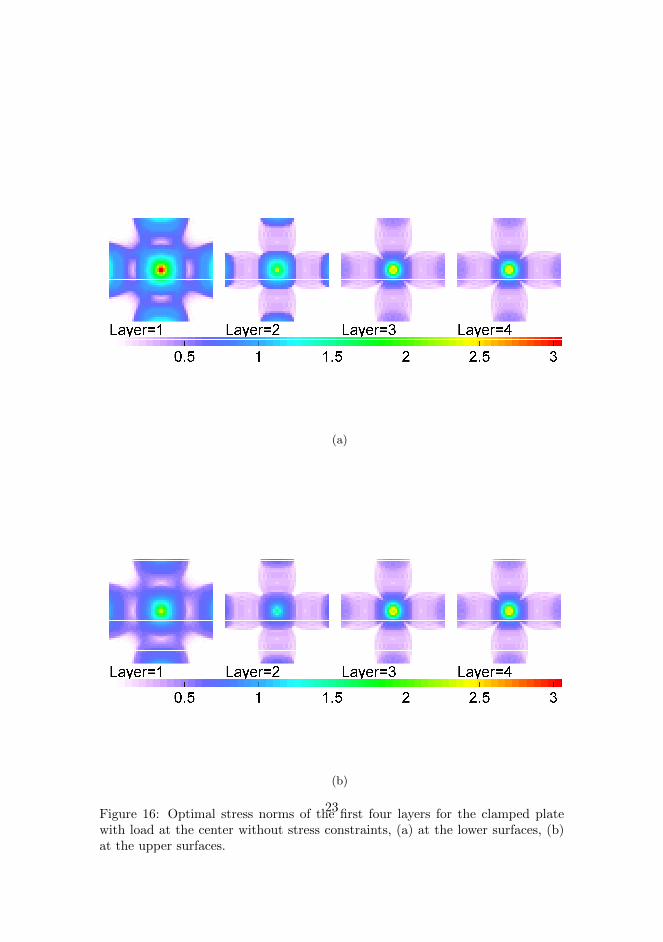
(a)

(b)

Figure 16: Optimal stress norms of the first four layers for the clamped platewith load at the center without stress constraints, (a) at the lower surfaces, (b)at the upper surfaces.

23

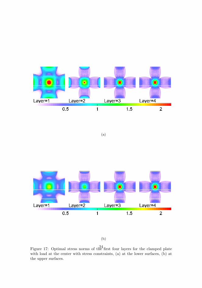
(a)

(b)

Figure 17: Optimal stress norms of the first four layers for the clamped platewith load at the center with stress constraints, (a) at the lower surfaces, (b) atthe upper surfaces.

24

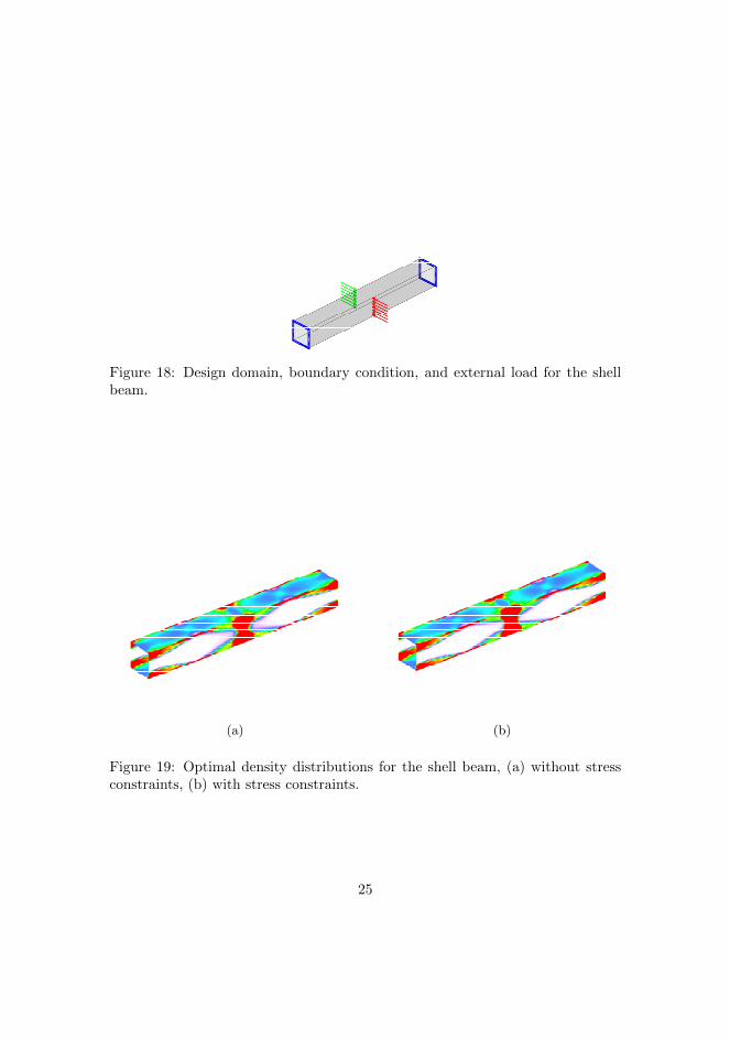
Figure 18: Design domain, boundary condition, and external load for the shellbeam.

(a) (b)

Figure 19: Optimal density distributions for the shell beam, (a) without stressconstraints, (b) with stress constraints.

25

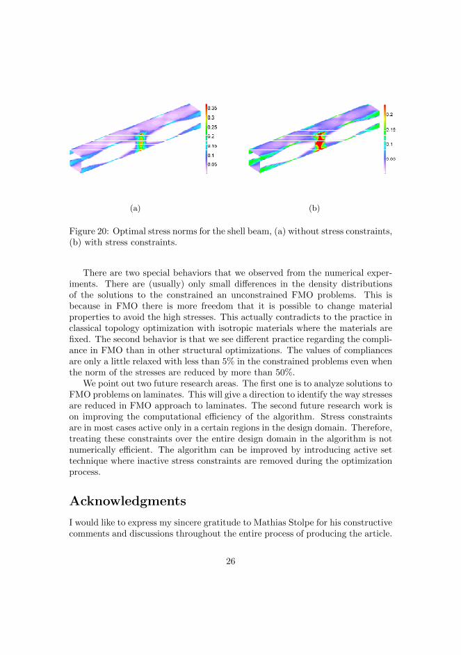
(a) (b)

Figure 20: Optimal stress norms for the shell beam, (a) without stress constraints,(b) with stress constraints.

There are two special behaviors that we observed from the numerical exper-iments. There are (usually) only small differences in the density distributionsof the solutions to the constrained an unconstrained FMO problems. This isbecause in FMO there is more freedom that it is possible to change materialproperties to avoid the high stresses. This actually contradicts to the practice inclassical topology optimization with isotropic materials where the materials arefixed. The second behavior is that we see different practice regarding the compli-ance in FMO than in other structural optimizations. The values of compliancesare only a little relaxed with less than 5% in the constrained problems even whenthe norm of the stresses are reduced by more than 50%.

We point out two future research areas. The first one is to analyze solutions toFMO problems on laminates. This will give a direction to identify the way stressesare reduced in FMO approach to laminates. The second future research work ison improving the computational efficiency of the algorithm. Stress constraintsare in most cases active only in a certain regions in the design domain. Therefore,treating these constraints over the entire design domain in the algorithm is notnumerically efficient. The algorithm can be improved by introducing active settechnique where inactive stress constraints are removed during the optimizationprocess.

Acknowledgments

I would like to express my sincere gratitude to Mathias Stolpe for his constructivecomments and discussions throughout the entire process of producing the article.

26

My special thanks also go to my colleagues Jose Pedro Blasques and RobertBitsche for many and fruitful discussions on laminated composite structures.

References

[1] Achtziger, W., Kanzow, C.: Mathematical programs with vanishing con-straints. Mathematical Programming 114(1), 69–99 (2008)

[2] Bendsøe, M.P., Dıaz, A.R.: Optimization of material properties for Mindlinplate design. Structural Optimization 6, 268–270 (1993)

[3] Bendsøe, M.P., Guedes, J.M., Haber, R.B., Pedersen, P., Taylor, J.E.: Ananalytical model to predict optimal material properties in the context ofoptimal structural design. Journal of Applied Mechanics 61, 930–937 (1994)

[4] Chapelle, D., Bathe, K.J.: The Finite Element Analysis of Shells - Funda-mentals. Springer, Heidelberg (2003)

[5] Cheng, G.D., Guo, X.: ε-relaxed approach in structural topology optimiza-tion. Structural Optimization 13, 258–266 (1997)

[6] Cook, R.D., Malkus, D.S., Plesha, M.E., Witt, R.J.: Concepts and Applica-tions of Finite Element Analysis, 4th edn. John Wiley and Sons (2002)

[7] Duysinx, P., Bendsøe, M.P.: Topology optimization of continuum structureswith local stress constraints. International Journal for Numerical Methodsin Engineering 43, 1453–1478 (1998)

[8] Forsgren, A.: Inertia-controlling factorizations for optimization algorithms.Applied Numerical Mathematics 43, 91–107 (2002)

[9] Gaile, S.: Free material optimization for shells and plates. Ph.D. thesis, Insti-tute of Applied Mathematics II, Friedrich-Alexander University of Erlangen-Nuremberg (2011)

[10] Guo, X., Cheng, G., Yamazaki, K.: A new approach for the solution ofsingular optima in truss topology optimization with stress and local buck-ling constraints. Structural and Multidisciplinary Optimization 22, 364–372(2001)

[11] Haslinger, J., Kocvara, M., Leugering, G., Stingl, M.: Multidisciplinary freematerial optimization. SIAM Journal on Applied Mathematics 70(7), 2709–2728 (2010)

27

[12] Hinton, M.J., Kaddour, A.S., Soden, P.D.: Failure criteria in fibre reinforcedpolymer composites: The world-wide failure exercise. Elsevier, Oxford, UK(2004)

[13] Kirsch, U.: On singular topologies in optimum structural design. StructuralOptimization 2, 133–142 (1990)

[14] Kocvara, M., Stingl, M.: A code for convex nonlinear and semidefinite pro-gramming. Optimization Methods and Software 18(3), 317–333 (2003)

[15] Kocvara, M., Stingl, M.: Free material optimization for stress constraints.Structural and Multidisciplinary Optimization 33, 323–355 (2007)

[16] Kocvara, M., Stingl, M.: Mathematical models of FMO with stress con-straints FMO. Tech. rep., PLATO-N Public Report PU-R-1-2008 (2009).Available from http://www.plato-n.org/

[17] Kocvara, M., Stingl, M., Zowe, J.: Free material optimization: recentprogress. Optimization 57(1), 79–100 (2008)

[18] Le, C., Norato, J., Bruns, T., Ha, C., Tortorelli, D.: Stress-based topologyoptimization for continua. Structural and Multidisciplinary Optimization41, 605–620 (2010)

[19] Nocedal, J., Wright, S.J.: Numerical Optimization. Springer, NewYork, NY,USA (1999)

[20] Parıs., J., Navarrina, F., Colominas, I., Casteleiro, M.: Topology optimiza-tion of continuum structures with local and global stress constraints. Struc-tural and Multidisciplinary Optimization 39(4), 419–437 (2009)

[21] Reddy, J.: Mechanics of laminated composite plates and shells: theory andanalysis, 2nd edn. London (2004)

[22] Ringertz, U.T.: On finding the optimal distribution of material properties.Structural Optimization 5, 265–267 (1993)

[23] Rozvany, G.I.N.: Difficulties in truss topology optimization with stress, localbuckling and system stability constraints. Structural Optimization 11, 213–217 (1996)

[24] Stingl, M.: On the solution of nonlinear semidefinite programs by aug-mented lagrangian method. Ph.D. thesis, Institute of Applied MathematicsII, Friedrich-Alexander University of Erlangen-Nuremberg (2006)

28

[25] Stingl, M., Kocvara, M., Leugering, G.: Free material optimization withfundamental eigenfrequency constraints. SIAM Journal on Optimization20(1), 524–547 (2009)

[26] Stingl, M., Kocvara, M., Leugering, G.: A new non-linear semidefinite pro-gramming algorithm with an application to multidisciplinary free materialoptimization. International Series of Numerical Mathematics 158, 275–295(2009)

[27] Stingl, M., Kocvara, M., Leugering, G.: A sequential convex semidefiniteprogramming algorithm with an application to multiple-load free materialoptimization. SIAM Journal on Optimization 20(1), 130–155 (2009)

[28] Stingl, M., Kocvara, M., Leugering, G.: A sequential convex semidefiniteprogramming algorithm with an application to multiple-load free materialoptimization. SIAM Journal on Optimization 20(1), 130–155 (2009)

[29] Stolpe, M., Svanberg, K.: On the trajectories of the epsilon-relation relax-ation approach for stress-constrained truss topology optimization. Structuraland Multidisciplinary Optimization 21, 140–151 (2001)

[30] Stolpe, M., Svanberg, K.: A note on tress-based truss topology optimization.Structural and Multidisciplinary Optimization 25, 62–64 (2003)

[31] Wachter, A., Biegler, L.T.: On the implementation of an interior-point filterline-search algorithm for large-scale nonlinear programming. MathematicalProgramming 106, 25–57 (2006)

[32] Weldeyesus, A.G., Stolpe, M.: Free material optimization for laminatedplates and shells. Tech. rep., DTU Wind Energy (2014). Submitted

[33] Weldeyesus, A.G., Stolpe, M.: A primal-dual interior point method for large-scale free material optimization. Computational Optimization and Applica-tions (2014). DOI 10.1007/s10589-014-9720-6

[34] Werner, R.: Free material optimization-mathematical analysis and numer-ical solution. Ph.D. thesis, Institute of Applied Mathematics II, Friedrich-Alexander University of Erlangen-Nuremberg (2001)

[35] Yang, B.J., Chen, C.J.: Stress-based topology optimization. Structural Op-timization 12, 98–105 (1996)

[36] Zowe, J., Kocvara, M., Bendsøe, M.P.: Free material optimization via math-ematical programming. Mathematical Programming 79, 445–466 (1997)

29

Chapter 8

On solving Free MaterialOptimization problemsusing iterative methods

Stolpe, M., Weldeyesus, A.G.: On solving Free Material Optimization problemsusing iterative methods. Department of Wind Energy, Technical University ofDenmark, 2014. To be submitted.

114

On solving Free Material Optimization problems

using iterative methods

Mathias Stolpe∗ and Alemseged Gebrehiwot Weldeyesus†

Abstract

Free Material Optimization (FMO) is concerned with obtaining the opti-mal material distribution and the optimal local material properties of a loadbearing structures. The problems are formulated with the stiffness tensortaken as design variable. These formulations lead to large scale nonlin-ear semidefinite programming problems for which specialized and efficientmethods are usually preferred. The authors have developed a primal-dualinterior point method in which the saddle point systems for obtaining thesearch directions are solved using direct solvers. This requires large mem-ory and restricts the size of the problems that can solved. The goal of thisarticle is to introduce iterative solvers to the method. Two different precon-ditioners are proposed and they are evaluated by solving several large-sclae3D problems.

Mathematics Subject Classification 2010: 90C22, 90C90, 74P05, 74P15

Keywords: Structural optimization, free material optimization, semidefinite op-timization, iterative methods

1 Introduction

Free Material Optimization (FMO) is branch of structural optimization in whichwe search for the optimal material distribution and the optimal local material

The research was partially funded by the Danish Council for Strategic Research throughthe Danish Center for Composite Structures and Materials (DCCSM).∗DTU Wind Energy, Technical University of Denmark, Frederiksborgvej 399, 4000 Roskilde,

Denmark. E-mail: matst@dtu.dk†DTU Wind Energy, Technical University of Denmark, Frederiksborgvej 399, 4000 Roskilde,

Denmark. E-mail: alwel@dtu.dk

1

properties. The basic formulations were studied in the early 1990s in [2], [3], and[20]. Throughout the last two decades FMO has been studied in several articles.Current FMO models have been extended to treat a wide range of constraintssuch as limits on stresses, strains, displacement, and fundamental frequenciesin e.g. [16], [14], [12], and [23]. The models are further extended to problemson curved thin-wall structures in [9] and to laminated structures in [29]. FMOtheories focusing on existence of optimal solutions have been analyses in severalarticle, see e.g. [12] and [31].

The design variable in FMO is the stiffness tensor which is allowed to vary ateach point of the design domain but forced to be symmetric and positive semidef-inite. Hence, the problems are classified as nonlinear semidefinite programs. Var-ious methods have been proposed for solving FMO problems. These include amethod based on penalty/barrier multipliers (PBM) in [34] and a method basedon augmented Lagrangian function in [13] and [22], a method based on a sequen-tial convex programming concept [25, 24], and a method based on interior pointmethods [30]. Second-order methods, such as interior point methods, for solvinglarge-scale FMO problems demand typically large memory. In order to cope withthis challenge it is important that iterative solvers are employed to the methods.In none of the methods and articles listed above the use of iterative solvers isexplicitly described.

The main challenge in using iterative solvers is the development of an efficientpreconditioners. The extent of the challenge is even worse in optimization meth-ods since the saddle-point system that needs to be solved becomes more and moreill-conditioned as the iterates are closing in on the optimal solution. Various pre-conditioners have been proposed for linear and convex quadratic programming,see [1] and [19], and for nonlinear optimization problems, see [7] and [5] and thereferences therein. The optimization problems arising form FMO belong to aclass optimization called (nonlinear) SemiDefinite Programming (SDP). In [8],[27], [28], and [33] iterative solvers have been used for solving linear SDP prob-lems. For the method based on augmented Lagrangian function in [13] iterativesolvers are introduced in [15]. The method has solved a set of SDP problems. Itis claimed in [22], [14], and [16] that it has been also used to solve FMO problemswith no report on related numerical statistics. However, in [25] it is pointed outthat the success is moderate.

The objective of this article is to introduce iterative solvers to the saddle-pointsystem in the primal-dual interior point method in [30]. The method in [30] hasappealing numerical behavior. It efficiently utilizes the problem structure thateach of the matrix inequalities involves small size matrix. It has obtained highquality solutions to large two-dimensional FMO problems within modest numberof iterations that is almost independent to problem size.

Notation: For (d1, d2, . . . , dm) ∈ Nm let S = Sd1 × Sd2 × · · · × Sdm where

2

Sdi be the space of symmetric di × di matrices. We denote by Sdi+ the cone of

positive semidefinite matrices Sdi , i.e., Ei ∈ SN+ if and only if Ei = ETi and

Ei 0. We define the operator T1 : S → Rm by (T1E)i = Tr(Ei) and theoperator T2 : S → R by T2E =

∑i Tr(Ei) for every E = (E1, . . . , Em)T ∈ S.

The adjoints of these operators are T ∗1 : Rm → S defined by (T ∗1 y)i = yiI forevery y ∈ Rm and T ∗2 : R → S defined by (T ∗2 α)i = αI for every α ∈ R wherethe identity matrix I in both cases has the same size as Ei. For some non-singular matrix P ∈ Rn×n is the linear operator HP

1 : Rn×n → Sn is defined byHP (Q) := 1

2

(PQP−1 + (PQP−1)T

). The operator P Q : Sn → Sn is defined

by (P Q)K := 12 (PKQT +QKPT ).

2 Problem formulations

We consider the discrete version of the minimum compliance (maximum stiffness)FMO problem formulation described in most of todays articles. For the prob-lem formulation in function space and related mathematical treatments such asexistence of solution, see the recent article [12] and the references there in.

We consider a design domain Ω which is partitioned into m uniform elements.The stiffness tensor E(x) is function constant on each element such that theelement values constituting the vector of block matrices E = (E1, . . . , Em)T . Fora given static load vector f ∈ Rn the associated displacement satisfies the linearelastic equilibrium equation

A(E)u = f (1)

where A(E) ∈ Rn×n is the global stiffness matrix.The most common quantity used in FMO to measure stiffness is the trace of

the stiffness tensor. Arbitrary local stiffness and extreme softness are controlledby introducing a local upper bound ρ and a lower bound ρ on the trace of thestiffness tensor. These bounds are assumed to satisfy 0 ≤ ρ < ρ < ∞. For therequirement of the physical attainability of the stiffness tensor is introduced bymatrix inequality constraints. We then define the set of admissible materials by

E :=E ∈ (Sd+)m | ρe ≤ T1E ≤ ρe

(2)

where e = (1, 1, . . . , 1)T is a vector of all ones of appropriate size and d = 3for two-dimensional problems and d = 6 for three-dimensional problems. Theamount of available resource material is described by T2E and this should not

1 This was introduced in [32]. Moreover, it is shown that HP (Q) = µI ⇔ Q = µI for ascalar µ.

3

exceed the volume fraction V satisfying the relation

m∑

i=1

ρ < V <

m∑

i=1

ρ.

The basic single load minimum compliance FMO problem is the formulatedas

minimizeu∈Rn,E∈E

fTu

subject to A(E)u = f

T2E ≤ V.(3)

The problem formulation (3) has a linear objective function, linear matrixinequalities and nonlinear (and nonconvex) vector constraints. Hence, it is clas-sified as nonconvex SDP problems.

3 The barrier problem and optimality condition

This section, which presents parts of the interior point method, is essentiallyidentical to Section 4 of [30] and is included for completeness. We introduce theslack variables (r, r, s) ∈ Rm

+ ×Rm+ ×R+ and barrier parameter µ > 0 to problem

(3) and formulate the associated barrier problem as

minimizeu∈Rn,E∈E,r,r,s

fTu− µm∑

i=1

ln(det(Ei))− µm∑

i=1

ln(ri)− µm∑

i=1

ln(ri)− µ ln(s)

subject to A(E)u− f = 0,

T1E + r − ρe = 0,

ρe− T1E + r = 0,

T2E + s− V = 0.(4)

The strict positivity of the slack variables is implicitly understood in the loga-rithmic functions. The barrier problem (4) has the following Lagrange function

L(x) =fTu− µm∑

i=1

ln(det(Ei))− µm∑

i=1

ln(ri)− µm∑

i=1

ln(ri)− µ ln(s)

+ λT (A(E)u− f) + βT (T1E + r − ρe)

+ βT (ρe− T1E + r) + α(T2E + s− V ),

(5)

4

where x = (E, u, r, r, s, λ, β, β, α) and (λ, β, β, α) ∈ Rn × Rm+ × Rm

+ × R+ areLagrange multipliers. The first-order optimality conditions to problem (4) are

λTF (u)− Z + T ∗1 β − T ∗1 β + T ∗2 α = 0 (6a)

A(E)λ+ f = 0 (6b)

A(E)u− f = 0 (6c)

T1E + r − ρe = 0 (6d)

ρe− T1E + r = 0 (6e)

T2E + s− V = 0 (6f)

RB − µe = 0 (6g)

R B − µe = 0 (6h)

sα− µ = 0 (6i)

HP (EZ)− µI = 0 (6j)

whereB = diag(β), B = diag(β), R = diag(r), R = diag(r),

and F (u) = (A1(E)j,ku, . . . , Am(E)j,ku) with Ai(E)j,k = ∂Ai(E)∂(Ei)j,k

and the multi-

plication λTF (u) defined such that (λTF (u))i = λTAi(E)j,ku for each j and kin the set of indices of Ei. The complementarity equation (6j) appearing in theoptimality conditions is the result of setting Z := µE−1 in equation (6a). Theapplication of the operator Hp is to ensure symmetry of the product EZ. Thedirections obtained by various choices of P are of the Monteiro-Zhang (MZ) fam-ily [32]. We follow the recommendation made in [30] and use the NT direction[17, 18] obtained when P = W−1/2 with W = E1/2(E1/2ZE1/2)−1/2E1/2 for itsrobustness in solving FMO problems.

Under the assumption that E 0 the matrix A(E) is positive definite [25].The Lagrange multiplier λ is then uniquely determined is then adjoint equationA(E)λ+f = 0. This allows us to make the substitution λ = −u in (6a) and reducethe optimality conditions to the the primal residuals (6c)-(6f), the perturbedcomplementary conditions (6g)-(6j) and

−uTF (u)− Z + T ∗1 β − T ∗1 β + T ∗2 α = 0. (7)

Let Rd, (rp1 , . . . , rp4), and (rc1 , . . . , rc3 , Rc4) be the negative of the left handsides of (7), the negative of the primal residuals, and the negative of the perturbedcomplementary residuals respectively. We apply Newton’s method to the reducedsystem to compute the search directions. After making reductions by eliminating

5

∆β, ∆β, ∆r, ∆r, and ∆s as in (13) we obtain a reduced primal-dual system

− 1

2A(E) F (u) 0F (u)T D T ∗2

0 T2 −s/α

∆u∆E∆α

=

f −A(E)u

R1

r1

(8)

where D is a block diagonal matrix given by

D = F−1E + T ∗1 (R−1B +R−1B)T1, (9)

and R1 and r1 are given by

R1 = Rd + F−1Rc4 − T ∗1 R−1(rc1 − Brp2) + T ∗1 R−1(rc2 −Brp3) (10)

r1 = rp4 −1

αrc3 . (11)

Note that F (u)∆E =∑

i

∑j,k(Ai(E)j,ku)(∆Ei)j,k with j and k in the set of

indices of Ei.The block diagonal matrices E = E(E,Z) and F = F(E,Z) in (9) are the deriva-tives of HP (EZ) with respect to E and Z respectively and are determined by

E = P P−TZ and F = PE P−1 (12)

The search directions ∆β, ∆β, ∆r, ∆r, and ∆s are computed as

∆u = −2∆u (13a)

∆Z = F−1(Rc4 −∆E) (13b)

∆r = rp2− T1∆E (13c)

∆r = rp3+ T1∆E (13d)

∆β = R−1(rc1 + B(−rp2 + T1∆E)) (13e)

∆β = R−1(rc2 +B(−rp3− T1∆E)) (13f)

∆s =1

α(rc3 − s∆α). (13g)

where u in (13a) is introduced to make the coefficient matrix in (8) symmetric.

4 Preconditioners

The preconditioners proposed in this section are motivated by those proposed in[26] for solving large-scale variable thickness sheet problems. We start first with

6

constructing the preconditioner for the stiffness matrix A(E) based on the Sep-arate Displacement Component (SDC), see e.g. [11]. This is done by reorderingof the stiffness matrix A(E) as

A(E) =

Axx(E) Axy(E) Axz(E)Ayx(E) Ayy(E) Ayz(E)Azx(E) Azy(E) Azz(E)

(14)

and taking the taking the decoupling terms to define the SDC preconditionerP (E) by

P (E) = blkdiag(Axx(E), Ayy(E), Azz(E)). (15)

Based on the general theory in [4], we propose the block triangular preconditioner

PS =

− 1

2P (E) F (u) 0

0 S T ∗20 T2 −s/α

(16)

whereS = D + 2diag(F (u)T diag(P (E))−1F (u)) (17)

is an approximation of the Schur complement for the primal-dual system (8) andfor relatively large µ values, say µ > 10−4.

The preconditioner Ps in (16) is not effective when µ values are small andthe interior-point iterates approach an optimal solution. This is because the thesaddle-point system (8) becomes severely ill-conditioned at this point. For thiscase we go for a rather expensive approach that overcomes the ill-conditioningby employing perturbation in the block diagonal matrix D. This is done byintroducing the matrix

G = C +D (18)

where C is a given positive semidefinite (block) diagonal matrix. In the system(8) we multiply the second row by −F (u)G−1 and add it to the first row and by−T2G

−1 and add it to the third row. Moreover, we make the change of variable

∆E = G−1C∆E (19)

and rewrite the system (8) as

H F (u) bF (u)T DC−1G T ∗2bT T2 q

∆u

∆E∆α

=

f −A(E)u− F (u)G−1R1

R1

r1 − T2G−1R1

(20)

where

H = −(

1

2A(E) + F (u)G−1F (u)T

), b = −F (u)G−1T ∗2 , q = −(s/α+T2G

−1T ∗2 )

(21)

7

For the system (20) we propose the block triangular preconditioner

Qs =

H F (u) b

0 S11 S12

0 S21 S22

(22)

where

H = −(

1

2P (E) + F (u)G−1F (u)T

), S11 = DE−1G−diag(F (u)T diag(H)−1F (u))

S12 = T ∗2 − F (u)T diag(H)−1b, S22 = q − bT diag(H)−1b

For solving with H we expand the system to

(− 1

2P (E) F (u)F (u)T G

)(23)

and from numerical experiment point of view we suggest the preconditioner

(− 1

2P (E)− diag(F (u)TG−1F (u)) F (u)0 G

). (24)

We use preconditioned conjugate gradient method with incomplete Cholesky fac-torization for solving with the preconditioner P (E). We apply flexible GMRESto solve the systems (8), (20) and (23) where low tolerance is set for the lastsystem. For details on the Krylov subspace methods, see e.g. [21]. We employthe Sherman-Morrison formula [10] for solving with the blocks in the second andthird rows and columns of the preconditioners Ps and Qs.

5 The algorithm

In the primal-dual interior point method developed in [30] the barrier problem(4) needs to be solved for a sequence of barrier parameter µk monotonicallyconverging to zero. The solution of the barrier problem for sufficiently smallµ value corresponds to the solution of the original problem (3). The detail ofmethod is described in [30]. We present an overview of the method in Algorithm1 for compelteness.

6 Implementation and numerical experiments

The interior point method and the finite element routines are implemented inMATLAB. The standard eight-node hexahedral elements are considered with full

8

Algorithm 1 The primal-dual interior point algorithm described in [30]

Choose x0 and µ0.while stopping criteria for problem (3) is not satisfied do

while stopping criteria for problem (4) is not satisfied doCompute the search direction ∆xk by solving system (8) and (13).Compute step length α in two steps.

1. Compute the maximum possible step using fraction to the boundaryrule.

2. Perform a backtracking line search using the norm of the KKTsystem as merit function.Set the new iterate as xk+1 = xk + α∆xk.

end whileUpdate µk+1.

end while

Gaussian integration, see e.g. [6]. The optimality measure for solving the barrierproblem (4) is the norm of the optimality conditions. The optimality measure forsolving the original problem (4) is the norm of the optimality conditions measuredwithout perturbation on the complementarity conditions. The optimality andfeasibility tolerances are both set to 10−6 in the implementation. For startingpoint in the algorithm the design variable is set to E = 0.1ρI. The displacementand Lagrange multiplies for the equality constraints are set to zero. is set tou = 0. The slack variables and Lagrange multiplies for the inequality constraintsare set to ones or identity. The volume fraction is set to 40% of the maximumpossible weight. The local volume bounds are set to ρ = 1 and ρ = 10−5. Thematrix C in (18) is set to 0.01I.

If the number flexible GMRES iterations exceeds 70 for solving the system(8) with the preconditioner (16) then the algorithm is set to switch to solving thesystem (20) with the preconditioner (22). After making this switch the maximumnumber of flexible GMRES iterations for the first inner interior point iterations isset to 70 and for the next inner iterations to 20. This approach is not particularlyefficient (or pretty) and will be improved in the future.

For the numerical experiments we consider the three-dimensional problemsshown in Figure 1. The first problem is the classical Michell beam problem withdimensions 1× 2× 4 with lower side fixed and shear load at the top, see Figure1a. The second problem is the cantilever beam problem of dimensions 1×1×1.5fixed at the four corners of the lower side subjected to a tip load, see Figure 1b.In the third example the design domain is a bar stool of dimensions 1 × 1 × 1and is fixed at the four corners of the lower side and loaded at the middle of theupper side, see Figure 1c. There are three levels of finite element discretizations

9

(a) (b) (c)

Figure 1: Design domains, boundary conditions and loads for the Michell beamproblem (a), the Cantilever beam problem (b), the Bar stool problem (c).

for each of the design domains. In all cases the loads are applied over an area ofsize 0.2× 0.2. The problem instances are reported in Table 1.

We report the numerical results in Table 2 for the problems in Table 1. Themethod has obtained the optimal solutions for all problem instances satisfyingthe prescribed tolerances. The optimal density distributions are shown in Figure2. The behavior of the method is rather promising but not fully satisfactory.This can be seen from Figure 3 relating flexible GMRES iterations to interiorpoint iterations for the Michell beam problem. The plot shows that after certaininterior point iterations the method requires almost the maximum allowed num-ber of iterations for each first inner interior point iterations that is followed bymultiple inner interior point iterations. The switching µ values from using thepreconditioner (16) to using the preconditioner (22) for the problems Michell I,Michell II, and Michell III are 3.3e− 04, 1.3e− 06, and 1.1e− 03, respectively.

7 Conclusions

We introduce iterative solvers to the primal-dual interior point method in [30]and achieve preliminary numerical success. It was possible to obtain solution fora set of large-scale problems. However, the preconditioners proposed for solvingthe barrier problem that corresponds to small barrier parameter are expensiveand are not powerful enough. The research is an ongoing study and is in its early

10

(a) (b)

(c)

Figure 2: Optimal density distribution for the Michell beam problem (a), theCantilever beam problem (b), the Bar stool problem (c).

11

0 5 10 15 20 25 30 350

10

20

30

40

50

60

70

80

90

Interior point iterations

flexi

ble

GM

RE

S it

erat

ions

Michell IMichell IIMichell III

Figure 3: Flexible GMRES iterations versus interior point iterations for theMichell beam problems.

Table 1: Problem instances.

Problem

No. of finite Total No. of No. of No. of non-elements of finite design fixed state

in each direction elements variables variables(Nx ×Ny ×Nz)

Michell I 8 × 16 × 32 4096 86016 14688Michell II 16 × 32 × 64 32768 688128 107712Michell III 32 × 64 × 128 262144 5505024 823680Cantilever I 16 × 16 × 16 4096 86016 14691Cantilever II 32 × 32 × 32 32768 688128 107619Cantilever III 64 × 64 × 64 262144 5505024 823443Bar stool I 16 × 16 × 16 4096 86016 14691Bar stool II 32 × 32 × 32 32768 688128 107619Bar stool III 64 × 64 × 64 262144 5505024 823443

stages. The main topics to work on will be the development of more efficientpreconditioners, theoretical explanations, and improved algorithmic strategies.

References

[1] Al-Jeiroudi, G., Gondzio, J., Hall, J.: Preconditioning indefinite systemsin interior point methods for large scale linear optimisation. Optimization

12

Table 2: Numerical results.

ProblemItn FGMRES itn. FGMRES itn. feas/opt

large µ small µ tolerances

Michell I 38 453 389 1.2e− 07/2.4e− 07Michell II 30 647 370 2.6e− 07/8.8e− 07Michell III 29 307 696 5.1e− 07/6.6e− 07Cantilever I 26 410 378 3.9e− 07/1.8e− 07Cantilever II 39 490 643 4.6e− 07/9.1e− 07Cantilever III 33 561 370 3.0e− 07/5.4e− 07Bar stool I 28 487 478 2.3e− 07/7.4e− 07Bar stool II 43 467 961 1.7e− 07/8.7e− 07Bar stool III 40 394 746 2.4e− 07/8.0e− 07

Methods and Software 23, 345–363 (2008)

[2] Bendsøe, M.P., Dıaz, A.R.: Optimization of material properties for Mindlinplate design. Structural Optimization 6, 268–270 (1993)

[3] Bendsøe, M.P., Guedes, J.M., Haber, R.B., Pedersen, P., Taylor, J.E.: Ananalytical model to predict optimal material properties in the context ofoptimal structural design. Journal of Applied Mechanics 61, 930–937 (1994)

[4] Benzi, M., Golub, G.H., Liesen, J.: Numerical solution of saddle point prob-lems. Acta Numerica 14, 1–137 (2005)

[5] Bergamaschi, L., Gondzio, J., Zilli, G.: Preconditioning indefinite systems ininterior point methods for optimization. Computational Optimization andApplications 28, 149–171 (2004)

[6] Cook, R.D., Malkus, D.S., Plesha, M.E., Witt, R.J.: Concepts and Applica-tions of Finite Element Analysis, 4th edn. John Wiley and Sons (2002)

[7] Forsgren, A., Gill, P.E., Griffin, D.J.: Iterative Solution of Augmented Sys-tems Arising in Interior Methods. SIAM Journal on Optimization 18, 666–690 (2007)

[8] Fukuda, M., Kojima, M., Shida, M.: Lagrangian dual interior-point methodsfor semidefinite programs. SIAM Journal on Optimization 12, 10071031(2002)

[9] Gaile, S.: Free material optimization for shells and plates. Ph.D. thesis, Insti-tute of Applied Mathematics II, Friedrich-Alexander University of Erlangen-Nuremberg (2011). Available from http://www.researchgate.net/

13

[10] Golub, G.H., van Loan, C.F.: Matrix Computations, 3rd edn. Johns HopkinsUniversity Press (1996)

[11] Gustafsson, I., Lindskog, G.: On parallel solution of linear elasticity prob-lems: Part I: theory. Numerical Linear Algebra with Applications 5(2),123–139 (1998)

[12] Haslinger, J., Kocvara, M., Leugering, G., Stingl, M.: Multidisciplinary freematerial optimization. SIAM Journal on Applied Mathematics 70(7), 2709–2728 (2010)

[13] Kocvara, M., Stingl, M.: A code for convex nonlinear and semidefinite pro-gramming. Optimization Methods and Software 18(3), 317–333 (2003)

[14] Kocvara, M., Stingl, M.: Free material optimization for stress constraints.Structural and Multidisciplinary Optimization 33, 323–355 (2007)

[15] Kocvara, M., Stingl, M.: On the solution of large-scale SDP problems by themodified barrier method using iterative solvers. Mathematical Programming120(1), 285–287 (2009)

[16] Kocvara, M., Stingl, M., Zowe, J.: Free material optimization: recentprogress. Optimization 57(1), 79–100 (2008)

[17] Nesterov, Y.E., Todd, M.J.: Self-scaled barriers and interior-point methodsfor convex programming. Mathematics of Operations Research 22(1), 1–42(1997)

[18] Nesterov, Y.E., Todd, M.J.: Primal-dual interior-point methods for self-scaled cones. SIAM Journal on Optimization 8(2), 324–364 (1998)

[19] Oliveira, A.R.L., Sorensen, D.: A new class of preconditioners for large-scalelinear systems from interior point methods for linear programming. LinearAlgebra and Its Applications 394, 1–24 (2005)

[20] Ringertz, U.T.: On finding the optimal distribution of material properties.Structural Optimization 5, 265–267 (1993)

[21] Saad, Y.: Iterative Methods for Sparse Linear Systems, Second Edition(2003)

[22] Stingl, M.: On the solution of nonlinear semidefinite programs by aug-mented lagrangian method. Ph.D. thesis, Institute of Applied MathematicsII, Friedrich-Alexander University of Erlangen-Nuremberg (2006). Availablefrom http://www2.am.uni-erlangen.de/

14

[23] Stingl, M., Kocvara, M., Leugering, G.: Free material optimization withfundamental eigenfrequency constraints. SIAM Journal on Optimization20(1), 524–547 (2009)

[24] Stingl, M., Kocvara, M., Leugering, G.: A new non-linear semidefinite pro-gramming algorithm with an application to multidisciplinary free materialoptimization. International Series of Numerical Mathematics 158, 275–295(2009)

[25] Stingl, M., Kocvara, M., Leugering, G.: A sequential convex semidefiniteprogramming algorithm with an application to multiple-load free materialoptimization. SIAM Journal on Optimization 20(1), 130–155 (2009)

[26] Stolpe, M., Weldeyesus, A.G.: On solving large-scale variable thickness sheetproblems. Tech. rep., DTU Wind Energy (2014). Submitted

[27] Toh, K.C.: Solving large scale semidefinite programs via an iterative solveron the augmented systems. SIAM Journal on Optimization 14(3), 670–698(2004)

[28] Toh, K.C., Kojima, M.: Solving some large scale semidefinite programs viathe conjugate residual method. SIAM Journal on Optimization 12, 669691(2002)

[29] Weldeyesus, A.G., Stolpe, M.: Free material optimization for laminatedplates and shells. Tech. rep., DTU Wind Energy (2014). Submitted

[30] Weldeyesus, A.G., Stolpe, M.: A primal-dual interior point method for large-scale free material optimization. Computational Optimization and Applica-tions (2014). DOI 10.1007/s10589-014-9720-6

[31] Werner, R.: Free material optimization-mathematical analysis and numer-ical solution. Ph.D. thesis, Institute of Applied Mathematics II, Friedrich-Alexander University of Erlangen-Nuremberg (2001)

[32] Zhang, Y.: On extending some primal-dual interior-point algorithms fromlinear programming to semidefinite programming. SIAM Journal on Opti-mization 8(2), 365–386 (1998)

[33] Zhao, X., D.Sun, Toh, K.C.: A Newton-CG augmented lagrangian methodfor semidefinite programming. SIAM Journal on Optimization 20(4), 1737–1765 (2010)

[34] Zowe, J., Kocvara, M., Bendsøe, M.P.: Free material optimization via math-ematical programming. Mathematical Programming 79, 445–466 (1997)

15

130