Models and Methods for Development of DSP Applications on ...
173
THESIS FOR THE DEGREE OF DOCTOR OF PHILOSOPHY Models and Methods for Development of DSP Applications on Manycore Processors Jerker Bengtsson School of Information Science, Computer and Electrical Engineering HALMSTAD UNIVERSITY Department of Computer Science and Engineering CHALMERS UNIVERSITY OF TECHNOLOGY G¨ oteborg, Sweden, June 2009
Transcript of Models and Methods for Development of DSP Applications on ...

THESIS FOR THE DEGREE OF DOCTOR OF PHILOSOPHY
Models and Methods for
Development of DSP
Applications on ManycoreProcessors
Jerker Bengtsson
School of Information Science, Computer and Electrical EngineeringHALMSTAD UNIVERSITY
Department of Computer Science and EngineeringCHALMERS UNIVERSITY OF TECHNOLOGY
Goteborg, Sweden, June 2009

ii
Models and Methods for Development of DSP Applications onManycore Processors
Jerker BengtssonISBN 978-91-7385-288-3
c© Jerker Bengtsson 2009.
Doktorsavhandlingar vid Chalmers tekniska hogskolaNy serie nr 2969ISSN 0346-718X
Department of Computer Science and EngineeringChalmers University of TechnologyTechnical Report No 62D.
Contact Information:
Department of Computer Science and EngineeringChalmers University of TechnologySE-412 96 Goteborg, SwedenTelephone: +46 (0)31 772 1000Fax: +46 (0)31 772 3663URL: http://www.ce.chalmers.se
School of Information Science,Computer and Electrical EngineeringHalmstad UniversityBox 823 SE-301 18 Halmstad, SwedenTelephone: +46(0)35 16 71 00Fax: +46(0)35 12 03 48URL: http://www.hh.se/ide
Printed by Chalmers ReproserviceGoteborg, Sweden, Maj 2009.

iii
Abstract
Advanced digital signal processing systems require specialised high-performanceembedded computer architectures. The term high-performance translates tolarge amounts of data and computations per time unit. The term embeddedfurther implies requirements on physical size and power efficiency. Thus therequirements are of both functional and non-functional nature.
This thesis addresses the development of high-performance digital signalprocessing systems relying on manycore technology. We propose building two-level hierarchical computer architectures for this domain of applications. Fur-ther, we outline a tool flow based on methods and analysis techniques forautomated, multi-objective mapping of such applications on distributed mem-ory manycore processors. In particular, the focus is put on how to provide ameans for tunable strategies for mapping of task graphs on array structureddistributed memory manycores, with respect to given application constraints.We argue for code mapping strategies based on predicted execution perfor-mance, which can be used in an auto-tuning feedback loop or to guide manualtuning directed by the programmer.
Automated parallelization, optimisation and mapping to a manycore pro-cessor benefits from the use of a concurrent programming model as the start-ing point. Such a model allows the programmer to express different types andgranularities of parallelism as well as computation characteristics of impor-tance in the addressed class of applications. The programming model shouldalso abstract away machine dependent hardware details. The analytical studyof WCDMA baseband processing in radio base stations, presented in this the-sis, suggests dataflow models as a good match to the characteristics of theapplication and as execution model abstracting computations on a manycore.
Construction of portable tools further requires a manycore machine modeland an intermediate representation. The models are needed in order to decou-ple algorithms, used to transform and map application software, from hard-ware. We propose a manycore machine model that captures common hardwareresources, as well as resource dependent performance metrics for parallel com-putation and communication. Further, we have developed a multi-functionalintermediate representation, which can be used as source for code generationand for dynamic execution analysis.
Finally, we demonstrate how we can dynamically analyse execution usingabstract interpretation on the intermediate representation. It is shown thatthe performance predictions can be used to accurately rank different mappingsby best throughput or shortest end-to-end computation latency.
Keywords: parallel processing, manycore processors, high-performance digitalsignal processing, dataflow, concurrent models of computation, parallel codemapping, parallel machine model, dynamic performance analysis.

iv
Sammanfattning
Avancerade inbyggda signalbehandlingssystem kraver ofta specialiserade ochhogpresterande datorplattformar. Med hogpresterande menas att stora datavoly-mer och berakningsintensiva algoritmer maste processas inom ett begransattidsintervall. Inbyggda system har generellt oftast krav pa att understiga enviss fysisk storlek och att de maste vara energieffektiva.
Denna avhandling fokuserar pa anvandning av flerkarniga processorer forkonstruktion av hogpresterande signalbehandlingssystem. Vi foreslar en da-torarkitektur, i form av en tva-niva hierarki, for denna typ av signalbehndlings-system. Vidare presenterar vi ett verktygsflode baserat pa metoder och ana-lystekniker for automatiserad mappning av sadana tillampningar pa flerkarnigaprocessorer med distribuerat minne. Mer specifikt, vi fokuserar pa flexiblastrategier for kravstyrd mappning av berakningsgrafer pa flerkarniga proces-sorer organiserade i en tva-dimensionell matrisstruktur. Vi foresprakar automa-tiskt eller manuellt styrd reglering av mappingsdirektiv, dar beslut baseras paaterkoppling av prognostiserade exekveringsegenskaper.
Automatiserad parallellisering, optimering och mappning pa en flerkarnigprocessor kan forenklas avsevart genom att utga ifran en lamplig parallell pro-grammeringsmodell. En sadan modell tillater en programmerare att uttryckaolika typer och olika kornigheter av parallellism samt berakningskarakteristik,typiska for de typer av tillampningar som adresseras. En sadan programmer-ingsmodell maste ocksa abstrahera bort processorspecifika hardvarudetaljer.En analys av basbandsprocessning i WCDMA radiobasstationer, som presen-teras i denna avhandling, pekar ut dataflodesmodeller som mycket lampliga foratt programmera denna typ av tillampningar, samt som exekveringsmodellerfor program mappade pa flerkarniga processor.
For att kunna konstruera portabla utvecklingsverktyg kravs det en lampligmodell av flerkarniga processorer samt en mellanrepresentation. Processor-modellen behovs for att kunna utveckla maskinoberoende algoritmer for trans-formering och mappning av program. Vi foreslar en flerkarnig processormodellsom fangar typiska hardvaruresurser, saval som dess grundlaggande, parallellaberakningsoperationer. Vidare har vi utvecklat en multifunktionell mellanrep-resentation, vilken kan anvandas som utganspunkt for kodgenerering och fordynamisk exekveringsanalys.
Slutligen, denna avhandling visar ytterligare hur vi kan prognostisera dy-namiska programegenskaper vid exekvering pa flerkarniga processorer, genomatt tillampa abstrakt tolkning av mellanrepresentationen. Vi demonstrerar hurresultatet av dessa prognoser kan anvandas for att rangordna programmapp-ningar enligt bast periodisk genomstromning av data eller kortast svarstid.

v
Acknowledgements
There are several people who more or less have had some influence on mywork and the decisions I have made during the very crooked path leading tocompletion of this thesis.
My main supervisor Bertil Svensson (DuracellTM Inside) for his encour-agement, experienced advices and never fading enthusiasm and positiveness.Not to forget, for all the time (weekends and evenings) spent reading papers,reports and my theses produced during these years.
My assistant supervisor, Veronica Gaspes for providing constructive criti-cism, concrete inputs and suggestions, and for being a good source for moralsupport and advices in issues of non-functional character in life and work.
Professor Edward Lee, for hosting and inspiring me greatly and giving mevery valuable advices and suggestions during my very fruitful visit at Univer-sity of California at Berkeley. Also, thanks to Man-kit ”Jackie” Leung fordiscussing and providing solutions to problems that popped up during my firstclose encounter with Ptolemy and the code generator framework during mystay in Berkeley.
A large deal of this work has been done in various forms of cooperation anddiscussions with with Ericsson AB. I am very greatful to Anders Wass who gotthe leading role in the Ericsson relay race and hosted me and spent valuabletime discussing and supporting me during and after my stays in Kista. Thebaton was later handed over to Henrik Sahlin and Peter Brauer who continuedguiding me through the LTE jungle, which greatly helped me when strugglingwith how to find an academic entry point to real problems, finding the rightlevels of abstraction and to obtain valuable insights into the industrial world.These industrial connections have provided me with a great deal of insightsand experiences which can only be read between the lines in this thesis.
Professor Marina Papatriantafilou, for being actively committed as externaladvisor in my support committee. Despite the limited room for meetings, therehas always been a positive and friendly attitude, and a good use of this limitedtime leading to useful outcome.
Roland Thorner, who have absolutely nothing at all to do with this thesis,but who is a very nice bloke and friend in his best years having a rarely goodsense of humor.
Finally, last but not least, my wife and constant brother in arms Hoai. Conkien cong con voi. Anh yeu em.
The work presented in this thesis has been funded by research grants form theKnowledge Foundation and Ericsson AB.

vi
Contents
Abstract iii
Acknowledgements v
Table of Contents vi
Lists of Appended Papers x
Other publications xi
1 INTRODUCTION 11.1 Microprocessor evolution: multicore versus manycore . . . . . . 21.2 High-performance digital signal processing . . . . . . . . . . . . 21.3 Scope of the thesis . . . . . . . . . . . . . . . . . . . . . . . . . 31.4 Problem description . . . . . . . . . . . . . . . . . . . . . . . . 41.5 Research goals and approach . . . . . . . . . . . . . . . . . . . 51.6 Contributions of the thesis . . . . . . . . . . . . . . . . . . . . . 61.7 Outline of the thesis . . . . . . . . . . . . . . . . . . . . . . . . 8
2 HIERARCHICAL ARCHITECTURE FOR EMBEDDED HIGH-PERFORMANCE SIGNAL PROCESSING 112.1 Embedded high-performance DSP systems . . . . . . . . . . . . 122.2 A hierarchical manycore architecture . . . . . . . . . . . . . . . 132.3 Reconfigurable micro level structures . . . . . . . . . . . . . . . 132.4 Evaluation of a reconfigurable micro level structure . . . . . . . 15
2.4.1 Evaluating area performance . . . . . . . . . . . . . . . 162.4.2 Evaluating resource utilisation . . . . . . . . . . . . . . 18
2.5 Implications for the further work . . . . . . . . . . . . . . . . . 19
3 ANALYSIS OF WCDMA BASEBAND PROCESSING 213.1 WCDMA and the UTRAN architecture . . . . . . . . . . . . . 22
3.1.1 The RBS . . . . . . . . . . . . . . . . . . . . . . . . . . 22

viii Contents
3.1.2 Downlink transport channel multiplexing . . . . . . . . 233.2 Downlink processing analysis . . . . . . . . . . . . . . . . . . . 23
3.2.1 Types of parallelism . . . . . . . . . . . . . . . . . . . . 25
3.2.2 Real-time characteristics . . . . . . . . . . . . . . . . . . 25
3.2.3 Parameter configuration . . . . . . . . . . . . . . . . . . 26
3.2.4 Function level parallelism . . . . . . . . . . . . . . . . . 273.2.5 Intra function characteristics . . . . . . . . . . . . . . . 27
3.2.6 3G service use cases . . . . . . . . . . . . . . . . . . . . 28
3.2.7 Mapping study of the use cases . . . . . . . . . . . . . . 29
3.3 Summary and implications . . . . . . . . . . . . . . . . . . . . 30
4 STREAMING MODELS OF COMPUTATION 31
4.1 Introduction . . . . . . . . . . . . . . . . . . . . . . . . . . . . . 32
4.1.1 Domain specific programming solutions . . . . . . . . . 32
4.1.2 Stream processing . . . . . . . . . . . . . . . . . . . . . 33
4.2 Synchronous dataflow . . . . . . . . . . . . . . . . . . . . . . . 34
4.2.1 Description of SDF . . . . . . . . . . . . . . . . . . . . . 354.3 StreamIt: a language implementing SDF . . . . . . . . . . . . . 37
4.3.1 Limitations in StreamIt . . . . . . . . . . . . . . . . . . 37
4.4 A modelling framework for SDF languages . . . . . . . . . . . . 38
4.4.1 The StreamBits language . . . . . . . . . . . . . . . . . 38
4.5 Related work . . . . . . . . . . . . . . . . . . . . . . . . . . . . 39
5 MACHINE MODEL, INTERMEDIATE REPRESENTATIONAND ABSTRACT INTERPRETATION 41
5.1 Manycore code mapping tool . . . . . . . . . . . . . . . . . . . 425.1.1 Target processors . . . . . . . . . . . . . . . . . . . . . . 43
5.2 Model set . . . . . . . . . . . . . . . . . . . . . . . . . . . . . . 44
5.2.1 Application model . . . . . . . . . . . . . . . . . . . . . 44
5.2.2 Machine model . . . . . . . . . . . . . . . . . . . . . . . 45
5.3 Timed configuration graphs . . . . . . . . . . . . . . . . . . . . 46
5.3.1 Construction of timed configuration graphs . . . . . . . 475.4 Abstract interpretation of timed configuration graphs . . . . . 47
5.4.1 Interpretation using Process Network . . . . . . . . . . 48
5.4.2 Modelling limitations of the IR . . . . . . . . . . . . . . 50
5.5 Evaluating modelling accuracy . . . . . . . . . . . . . . . . . . 50
5.5.1 Experimental mapping cases . . . . . . . . . . . . . . . 515.5.2 Execution strategy . . . . . . . . . . . . . . . . . . . . . 52
5.5.3 Comparing communication costs . . . . . . . . . . . . . 52
5.5.4 Latency and throughput measurements . . . . . . . . . 54
5.6 Discussion of the results . . . . . . . . . . . . . . . . . . . . . . 56
5.7 Related work . . . . . . . . . . . . . . . . . . . . . . . . . . . . 57

Contents ix
6 CONCLUSIONS AND FUTURE WORK 616.1 Conclusions . . . . . . . . . . . . . . . . . . . . . . . . . . . . . 626.2 Future work . . . . . . . . . . . . . . . . . . . . . . . . . . . . . 63
Bibliography 64
List of Figures 71
List of Tables 73

x Contents
Lists of Appended Papers
This thesis is based on the work contained in the following papers:
Paper A Johnsson, D., Bengtsson, J., and Svensson, B. (2004). Two-level re-configurable architecture for high-performance signal processing. In Proc.of Engineering of Reconfigurable Systems and Algorithms (ERSA’04),pages 177-183, Las Vegas, USA.
Paper B Bengtsson, J. (2006). Baseband processing in 3G UMTS radio basestations. Technical Report IDE0629, School of Information Science, Com-puter and Electrical Engineering, Halmstad University, 2006.
Paper C Bengtsson, J., and Svensson, B. (2006). A configurable frameworkfor stream programming exploration in baseband applications. In Proc.of The 11th Int’l Workshop on High-Level Programming Models AndSupportive Environments (HIPS’06) in conjunction with IPDPS (IPDPS2006), Rhodes, Greece.
Paper D Bengtsson, J. and Svensson, B. (2008). A domain-specific approachfor software development on manycore platforms. ACM Computer Ar-chitecture News, Special Issue: MCC08 - Multicore Computing 2008,39(6):2-10.
Paper E Bengtsson, J., and Svensson, B. (2009). Manycore performance anal-ysis using timed configuration graphs. To appear in Proc of. Int’l Symp.on Systems, Architectures, Modeling and Simulation (SAMOS IX 2009),Samos, Greece.

Contents xi
Other Related Publications
Bengtsson, J. (2006a). Efficient Implementation of Stream Applications onProcessor Arrays. Licentiate Thesis, Chalmers University of Technology,March 30, 2006.
Bengtsson, J., Gaspes, V., and Svensson, B. (2007). Machine assisted codegeneration for manycore processors. Real-time in Sweden, Vasteras (RTIS2007).
Bengtsson, J. and Svensson, B. (2008a). A set of models for manycore perfor-mance evaluation through timed configuration graphs. Technical ReportIDE0856, School of Information Science, Computer and Electrical Engi-neering, Halmstad University, 2008.
Bengtsson, J. and Svensson, B. (2008b). Methodologies and tools for devel-opment of signal processing software on multicore Platforms . Workshopon Streamings Systems in conjunction with 41st Annual IEEE/ACM In-ternational Symposium on Microarchitecture (MICRO 41).
Bengtsson, J., and Svensson, B. (2008c). A domain-specific approach forsoftware development on manycore platforms. In Proc. of First SwedishWorkshop on Multicore Computing (MCC08).

xii Contents

Chapter 1
INTRODUCTION

2 Introduction
1.1 Microprocessor evolution: multicore versus
manycore
The microprocessor industry has long been able to deliver increased perfor-mance of processors incited by Gordon Moore’s predictions. This has to alarge extent been possible through technology scaling of transistors and wires,continuously increased clock frequencies and adding more specialised functionalunits around a centralised processor architecture. However, an undesirable sideeffect of the technology scaling and the clock frequency race has been a rapidincrease in power dissipation, which started to push cooling technology to itslimit in the first years of 2000 [Carmean and Hall, 2001]. In 2005, Intel andAMD made a significant change in their directions on the chase for more powerefficient performance, starting from a single core architecture and then doublingthe amount of cores per semiconductor process generation. The term multicorehas become highly associated with this concept. There are many argumentsfor why this rather narrow minded design shift will unlikely be the ideal solu-tion for dramatic improvements in power performance [Asanovic et al., 2006].Sustainable and evolutionary solutions for parallel processing must be soughtfrom a broader perspective. As a response to this, the term manycore wascoined at the University of California at Berkeley to distinguish new and in-novative parallel processor architectures from the more limiting core doublingconvention.
1.2 High-performance digital signal processing
High-performance signal processing systems, such as advanced radar systems,has long required computer architectures capable of delivering performancelargely exceeding the performance of general purpose computer systems. Par-allel embedded computer architectures were early been a must to manage theprocessing requirements in such systems, and future generations will keep push-ing these requirements higher [Ahlander, 2007]. Another similar example is thesignal processing required in radio base stations (RBS). In practice, an RBS isa highly advanced parallel computer system. A state-of-the-art platform for 3GWCDMA RBSs is typically designed using the latest ASIC and FPGA tech-nologies to maximise the capability of serving as many number of concurrentlines as possible [Zhang et al., 2003]. Further, each RBS site typically containsmany such parallel platforms.
Although there are many dissimilarities between these two examples ofhigh-performance signal processing systems, there is at least one very impor-tant common denominator: development complexity and manufacturing cost.Radar systems are typically produced in smaller series, which makes the costper system for ASIC development very high. In the telecommunication indus-

1.3 Scope of the thesis 3
try, the production series are much longer, which therefore makes the ASIC costper system much lower compared to radars. However, the cost of developingASICs increases dramatically for each semiconductor technology generation.Furthermore, new and more complex functionality keeps being added to eachsystem generation. Thus, reducing manufacturing costs is one argument forindustry’s interest in using more commercial-of-the-shelf (COTS) manycorehardware.
Taking wireless telecommunication industry as example, the trend is that agrowing part of the baseband platforms are implemented using programmablehardware technology. An RBS typically has a life expectancy counted indecades. Using programmable technology enables performance upgrading andforward-compatibility; new standardised functionalities and improved algo-rithms can be integrated after system roll-out. Moreover, different customersneed different system solutions to meet their specific site requirements and havethe ability to modify the network with respect to communication. This putsfurther requirements on platform scalability.
1.3 Scope of the thesis
This thesis addresses a few of the many problems related to system and softwaredevelopment for using manycore technology in embedded computer architec-tures for high-performance signal processing applications. We focus on arraystructured, software cached, distributed memory manycore processors. We be-lieve that such machines provide good hardware scalability and good means forpredictable timing.
We address a certain class of high-performance digital signal processingsystems. We translate the term high-performance to real-time constrainedprocessing of large amounts of data and computation intensive algorithms. Wefocus on embedded systems, thus there are further requirements on physicalsize and power efficiency. Therefore, the requirements are of both functionaland non-functional nature. Applications that fit within this class are, e.g. base-band processing in radio base stations and signal processing in modern radarsystems. Applications not belonging to this class are, e.g. weather simulationsand scientific computations, since there typically is no strict requirements onresponse time.
Multi-processors have been widely explored in research since the 1980s andearly 1990s. There has also been a great deal of research on parallel program-ming models. We have focused on finding solutions for manycore programmingand code mapping based on this earlier work; more specifically, we have inves-tigated methods and techniques based on dataflow models of computation.
The problem of mapping task graphs to a parallel processing hardware iswell studied, and many solutions for automation of that problem exist. Given
4 Introduction
such a mapping, we focus on analysis techniques for the prediction of run-timeproperties of such task graphs on the category manycore targets addressed.
1.4 Problem description
We are interested in performance efficient DSP task graph mapping on highlyparallel, generic manycore hardware. We are especially interested in self-timedtask graph mappings, which put minimal requirements on run-time overheadfor execution on manycore hardware [Lee and Ha, 1989]. To find solutions tothis overall problem, we were motivated to address the following questions:
• What are the trade-offs concerning system development usingdifferent paradigms of manycore processors? Fine-grained many-cores with reconfigurable interconnections theoretically offer a larger areaperformance compared to more coarse-grained manycores. However, re-ducing core hardware implemented functionality means that a certainpart of the hardware resources must be used to configure correspondingfunctionality through software. Examples of such functionality can bememory address and cache logic and configuration of data paths (switch-ing/routing functionality). How does this strategy of moving certain func-tionality to software - normally implemented in hardware - impact onpractically achievable area performance?.
• What are the typical computation characteristics and process-ing requirements in embedded high-performance DSP systems?Embedded high-performance DSP systems typically contain large amountsof logical parallelism. These kinds of embedded systems are usually alsoassociated with a set of non-functional constraints, for example real-timeconstraints. Furthermore, the hardware resources must be shared formany concurrent processing tasks. To be able to determine requirementson programming models, target hardware and mapping strategies for suchhardware, it is necessary to analyse typical algorithm characteristics, log-ical parallelism etc. from a system perspective.
• What is a suitable parallel model of computation for DSP ap-plications? Automated mapping of application software requires well-defined parallel models of computation. Fewer and fewer are those whostill believe that the non-concurrent, shared memory programming modeloffered by the C language is a good starting point for automated map-ping to parallel hardware. A suitable parallel model of computation mustoffer concurrency but also provide means for manycore hardware indepen-dence.

1.5 Research goals and approach 5
• What is a suitable machine abstraction for manycore proces-sors? Tools and application software must be portable. This requiressuitable intermediate representations for modular tool building. Further,the target embedded systems are also associated with constraints of anon-functional nature. Thus, the optimisation of DSP task graphs tomanycore hardware is a complex, multi-objective task with many trade-offs. To deal with optimisation coupled to non-functional constraints, webelieve that such intermediate representations need to capture time andoffer means for analysis of dynamic execution costs.
1.5 Research goals and approach
The overall goals of this thesis work are:
1. to investigate trade-offs in signal processing implementation using differ-ent paradigms of manycore technology;
2. to investigate models, methods and techniques for computer assisted map-ping of signal processing task graphs on manycore hardware; and
3. to develop techniques for analysing and predicting dynamic executioncosts of DSP task graphs on manycores.
The research was initiated by studying and evaluating emerging manycorearchitectures [Bengtsson and Lundin, 2003]. To be able to analyse system de-sign trade-offs related to the choice of hardware technology, we later conducteda study on parts of the physical layer processing in 3G radio base stations.For the parts of the system studied, we found the synchronous dataflow modelof computation to offer a good match with the system and development re-quirements and with the manycore hardware addressed. Considering industrialrequirements on tool and software portability, we further addressed methodsand techniques for automated software mapping on parallel hardware. To ab-stract manycore hardware and to predict dynamic execution costs related tonon-functional properties, we identified the need for a new manycore machinemodel providing realistic execution cost predictions and a multi-functional in-termediate representation as an important research topic.

6 Introduction
1.6 Contributions of the thesis
The contributions of this thesis are as follows:
• Hierarchical processor architecture for high-performance signalprocessingWe propose a hierarchical manycore processor architecture for multi-dimensional signal processing platforms. We have investigated some ofthe trade-offs related to different core granularities by comparing twoparadigms of existing manycore processors: a coarse-grained array oftightly coupled RISC cores and a fine-grained reconfigurable array of sin-gle instruction ALUs. In the latter, both control flow and data operationsmust be mapped spatially using one or several of ALUs. Given a certainchip area and assuming the same technology, our comparisons show thatthe finer grained array has a potential peak performance of almost a factorof 7 higher than the coarse-grained processor. Furthermore, we studiedthe impact on performance when large amounts of ALU resources needto be allocated for algorithm control flow. Our experiments shows that,even if using up to as much as 75 percent of the ALUs for algorithmcontrol flow, it would still be competitive with the peak performance ofthe coarse-grained alternative.
• Processing requirements and characteristics in WCDMA base-bandWe provide a comprehensive study of the complete set of processing func-tions specified for 3G WCDMA downlink baseband. In the study, wemake an analysis of different types of potential parallelism. We discussthe functionality and characterise the intra-algorithm computations anddata representations. On the basis of the study, we find that stream-oriented models of computation constitute a very good match for describ-ing the task and the pipeline parallelism that we identify on the functionlevel in the WCDMA processing chain. On the intra-algorithm level, wealso identify and discuss potential mapping on SIMD and MIMD parallelhardware. Moreover, we conclude that the requirements on instruction-level computations are mostly of a logical, rather than an arithmetical,nature.
• Modelling framework for SDF based languagesWe provide a framework specialised for the modelling of stream-orientedlanguages based on the synchronous dataflow model of computation. Weused the StreamIt language in order to reason about implementation ofWCDMA downlink processing using stream-oriented languages. On thebasis of the WCDMA study, we identify a number of weaknesses related toexpressiveness in the StreamIt language and propose language extensions

1.6 Contributions of the thesis 7
related to data types and instruction level computations. Further, weintroduce the notion of a control mode - for periodical reconfigurationof actors - and control streams - for distribution of actor reconfigurationparameters. We demonstrate language improvements by modelling anexperimental language called StreamBits. In particular, we demonstratehow we can extend the StreamIt language with syntactic means to expresscomputations on variable length bit-string data types.
• Models for manycore performance evaluationWe developed a set of models to be used as a part of a manycore map-ping and code generation tool. Manycore processors are described usinga machine model that captures essential performance measures of arraystructured, tightly coupled manycore processors. Moreover, we developeda timed intermediate representation for manycore targets in the form ofa heterogeneous dataflow model. We show how the intermediate repre-sentation is constructed for abstract interpretation, given a model of theapplication (SDF) and a specification of the machine as input. Thus,the use of the timed intermediate representation is two-fold: 1) we canby means of abstract interpretation obtain feedback about the run-timebehaviour of the application and 2) we can use this IR as source for codegeneration to parallel targets.

8 Introduction
• Rank based feed back tuning using performance predictionsWe outline a design flow for iterative tuning of dataflow graphs on many-cores using predicted performance feed back. The tool has two purposes:1) to provide means for early estimates of application performance ona specific manycore and 2) to provide means for a programmer or anauto-tuner to tune mapping decisions on a manycore, based on feed backof predictions of a mapped application’s dynamical behaviour. We eval-uate the accuracy of the predictions calculated by our tool by makingcomparisons with measurements on the Raw processor. We show thatwe can fairly accurately predict both on-chip and off-chip communica-tion costs. Furthermore, we show with our experiments that the tool’spredictions can be used to correctly rank parallel mappings, by highestthroughput and shortest end-to-end latency, when tuning an applicationimplementation for such non-functional constraints.
1.7 Outline of the thesis
The thesis consists of two parts: a summary and a set of five appended papers.The six following chapters in the summary of the thesis are briefly summarisedbelow.
• Chapter 2 summarises our work on investigating a domain specific com-puter architecture for embedded high-performance digital signal process-ing. We outline and motivate our proposal of a two level hierarchicalarchitecture. Further, we make an analysis of area performance trade-offsassociated with the choice of manycore structure and its core granularity.
• Chapter 3 presents a study of downlink baseband processing in 3G radiobase stations. We summarise the function flow and its functional require-ments, the inter as well as intra-function characteristics and we identifypotential sources of logical parallelism. Further we discuss potential map-ping of baseband use cases on common types of parallel processors.
• Chapter 4 introduces stream processing and dataflow models of compu-tation in particular. Motivated by the baseband study in Chapter 3 andthe type of manycore architectures discussed in Chapter 2, we especiallyfocus on the synchronous dataflow model of computation. Furthermore,we briefly discuss data types and language constructions that we finduseful for implementing baseband processing in languages based on theSDF model of computation. Finally, we end the chapter by discussingrelated work on stream-oriented languages.
• Chapter 5 presents our work on models for abstracting manycores andDSP applications. We further propose a manycore intermediate represen-
1.7 Outline of the thesis 9
tation suitable for code generation and analysis of non-functional proper-ties of SDF graphs when mapped on a particular manycore. The chapteris finalized with related work on techniques and methods for mappingtask graphs on parallel processors. The chapter is ended by discussingfurther related work.
• Chapter 6 contains conclusions and suggestions for further work.

10 Introduction
Chapter 2
HIERARCHICAL
ARCHITECTURE FOR
EMBEDDED
HIGH-PERFORMANCE
SIGNAL PROCESSING

12 Architecture for Embedded High-performance Signal Processing
This chapter summarises our work on investigations of a domain specificcomputer architecture suited for embedded high-performance digital signal pro-cessing. We motivate and outline our proposal of a two level hierarchical archi-tecture. Further, we focus on analysing area performance trade-offs associatedwith the choice of computation structure and its granularity in the lower ab-straction level of our proposed architecture, as described in [Paper A].
2.1 Embedded high-performance DSP systems
We will first discuss some general system requirements that must typically beconsidered for a computer architecture for the targeted application domain.We discuss these requirements related to two examples of concrete applicationswithin this domain: signal processing in RBS and in radar systems.
Parallelism Embedded high-performance signal processing applications typ-ically consist of several types and granularities of parallelism. From asystem perspective, modern radars are developed to be capable of oper-ating in different modes and using multiple parallel antenna inputs. Inan RBS, the goal is to maximise the number of concurrent user channelshaving different requests on the types of services. The signal processingin a radar or an RBS constitutes pipelined function flows, exposing task,data and pipeline parallelism. Each function can further contain differentamounts of fine-grained instruction level parallelism. We aim for an ar-chitecture that is flexible and that can be dimensioned for heterogeneousparallelism of variable amounts.
Non-functional properties Both radar systems and radio base stations arereal-time systems. Thus, one important type of non-functional con-straints associated with such systems is time. New data are continuouslystreamed into the system by a certain periodicity (throughput) and itsoutput must be produced within a certain time (end-to-end latency). Asufficient mapping of a function flow must also fulfil the specified systemtiming requirements. We must be able to offer appropriate parallel map-ping strategies in order to process function flows of different structuresand with different computation loads, with respect to some given timingrequirements.
Scalability A set of, often computationally demanding, functions is applied onmulti-dimensional arrays of data collected from multiple antenna streams.Embedded high-performance systems are typically built using boardswith multiple chips and even using multiple boards. The sizes and thedimensions of the data shapes processed by the function flows typicallyvary depending on for example the radar task or the number of con-nected users and the specific services each is requesting from the wireless

2.2 A hierarchical manycore architecture 13
network. Thus, a domain specific computer architecture should be scal-able in order to enable the designer to dimension a system for differentrequirements.
System reconfiguration A system must be able to dynamically adapt to pe-riodically changing computation requirements. From a service schedulingpoint of view, the number of concurrent users and different types of ser-vice requests in an RBS can change frequently by a certain (often veryshort) periodicity. In practice, the size and the structure of the functionflows and the workload for each function change. Since these changes arenon-deterministic, the resource allocation must be done dynamically. Inconclusion, the computer architecture should be able to allow for fast re-configurations (dynamic resource allocation) of the processing resourcesto handle varying structures of the function flows and varying workloadsof the functions.
2.2 A hierarchical manycore architecture
In [Paper A], we propose a mesh structured computer architecture using a twolevel hierarchical abstraction: a macro level structure and a micro level struc-ture, see Figure 2.1. A mesh structure is easily scalable for different sizes ofparallel structures, both on chip level as well as on the board level. Further-more, the two level hierarchy provides an abstraction for both homogeneousand heterogeneous multiprocessor systems.
The macro level is a mapping abstraction for application and function levelparallelism. A macro node can very well abstract, for example, a programmablemanycore structure as well as a hardware implemented function accelerator.
The inside of a macro node constitutes the micro level structure. Dependingon the type of micro level structure, the architecture allows exploitation of fur-ther task, pipeline, data and instruction level parallelism, in order to computethe mapped functions as efficiently as required.
In our work, we have primarily focused our investigations on micro levelstructures in the form of homogeneous manycore technology. This choice offersa highly flexible mapping space and also simplifies programmability and codemapping.
2.3 Reconfigurable micro level structures
In the most recent decade there has emerged a variety of different kinds ofparallel and so called reconfigurable processor architectures. There is no welldefined taxonomy for categorisation of such processors. Neither is there a good

14 Architecture for Embedded High-performance Signal Processing
Figure 2.1: A two level manycore hierarchy. Macro level nodes can be eitherspecialised cores, dsp or, as illustrated by the figure, a micro level manycorestructure.
definition, in our opinion, of what clearly distinguishes a ”reconfigurable” pro-cessor from a ”programmable” processor. Instead, such processors are usuallycoarsely compared by the granularity of the processing elements (PE), how thePEs (or cores) are networked to form a parallel computing structure and howcomputations and the mapping of programs are done [Mangione-Smith et al.,1997].
The probably most explored and also most fine-grained of (re)configurablestructures are field programmable gate arrays (FPGA). However, such fine-grained bit-level structures tend to require large amounts of logic to implementarithmetic operations, such as multiplication, on word length data. This issuehas been addressed by the FPGA industry through embedding specialised wordlevel arithmetic units, such as multipliers, in the fine-grained FPGA logic.However, the reconfiguration times in FPGAs are very long and therefore notfitted for system requirements of fast run-time reconfiguration.
Word level reconfigurable manycore processors represent one class of in-teresting manycore processors for signal processing functions. Interestingly,research investigations have shown that it is possible to achieve performancescomparable with FPGAs for many applications requiring bit-level computa-tions [Wentzlaff and Agarwal, 2004].
Many parallel processors have been designed in the form of an array struc-ture, where the PEs (cores) are interconnected via a k-ary n-cubical network(that is, a network of n dimensions and k cores in each dimension). Consider-ing wire densities in VLSI implementations of such networks, it was shown byWilliam Dally in the early 1990s that low dimensional n-cubical networks yield

2.4 Evaluation of a reconfigurable micro level structure 15
lower communication latencies and higher hot spot throughput [Dally, 1990].Research has later also suggested that it can be possible to build and efficientlyutilise two dimensional array structures with thousands of coarse-grained cores[Moritz et al., 2001].
On the basis of these research findings and the characteristics of the appli-cation domain, which we described in Section 2.1, we have focused our intereston micro level structures in the form of mesh structured manycores.
2.4 Evaluation of a reconfigurable micro level
structure
Regarding the type and design of micro level nodes, the main issue is to choose amanycore structure that offers a mapping space flexible enough for exploitationof different types and levels of potential parallelism within different functions.There are several aspects to consider, for example:
• What are the area performance trade-offs with respect to core granular-ity?
• What are the functional requirements at the micro level nodes?
• What is the cost for implementing control flows and address logic?
In [Paper A] we mainly addressed these three aspects to get some indicativeanswers. We chose to compare two different categories of existing manycorestructures.
The first one, the XPP array architecture from PACT shown in Figure 2.2,is a homogeneous MISD (multiple instruction stream single data stream) arrayprocessor consisting of word length ALUs, which offers a spatial reconfigurablemapping space for algorithms [Baumgarte et al., 2001]. Using simple coreswithout instruction or data memory naturally enables a large amount of coresto be stamped out on a chip and thereby offers a large amount of instructionlevel parallelism. Similar to FPGAs, the array of cores must be reconfiguredto switch from one algorithm to another. Further, each type of ALU operationis performed within one clock cycle. The output from a computing core isavailable for its nearest neighbours in the proceeding clock cycle. The XPParray has on-chip data memory distributed over a set of memory elements.These elements can also be combined to form larger logical memories, offeringa larger address range when needed. The array has no dedicated controllerlogic to handle memory. Thus, memory read and write operations have to beimplemented using one or a set of ALUs.
The other, the Raw micro processor, shown in Figure 2.3, is a more coarse-grained MIMD (multiple instruction stream multiple data stream) array of

16 Architecture for Embedded High-performance Signal Processing
ALU ALU ALU Mem
ALU ALU ALU Mem
ALU ALU ALU Mem
ALU ALU ALU Mem
ALU ALU ALU I/O
ALU ALU
ALU ALU
ALU ALU
ALU ALU
ALU ALU
ALU ALU ALU I/OALU ALU
Mem
Mem
Mem
Mem
I/O
I/O
Array Configuration StorageConfig.
Controller
Figure 2.2: The figure illustrates the XPP dataflow processing array, which isa reconfigurable MISD type of manycore.
fewer (16) cores, compared to the XPP array, but offers both temporal and spa-tial mapping of algorithms [Taylor et al., 2002]. The cores are MIPS processorswith a slightly modified instruction set. Each core has instruction memory anda local (private) data cache. Moreover, Raw cores have floating point units.The cores are tightly coupled via four physical on-chip scalar operand networks- two statically and two dynamically routed - mapped via the register files. Thismeans that the network can be treated as source and destination operands ofan instruction (hence, the name scalar operand networks). The static networkrouters are programmable, so that static communication paths can be set upbetween cores. The dynamic networks are wormhole routed message passingnetworks, for core and memory communications of less deterministic nature.
2.4.1 Evaluating area performance
We have studied a specific implementation of the XPP array architecture - theXPP-64A - and the first prototype implementation of Raw. It is difficult tomake a fair area performance comparison between Raw and XPP-64A sincethey are of different types of architecture and are implemented in differentprocess technology. For example, large parts of the area for each Raw tile isused for the floating point unit and for larger local data caches (Raw has intotal 512 Kb compared to XPP’s 12 Kb) and the processors are implementedin different silicon processes. Raw cores use 32 bit word length, while XPP-64As ALUs have 24 bit word length. Furthermore, the Raw processor and the

2.4 Evaluation of a reconfigurable micro level structure 17
core core PE core
core PE PE PE
core core PE core
core core core core
Router
Instruction
mem
Data
mem
Instr. Sequencer
Reg
file
Figure 2.3: The figure illustrates the Raw micro processor, which is a MIMDtype of manycore array.
Processor Cores Area (mm2) Lithography (µm)
Raw 16 250 0.15XPP 64 32 0.13XPP Scaled 320 250 0.15
Table 2.1: Comparison of instruction level parallelism per area for Raw withXPP and the scaled XPP.
XPP-64A run at different clock frequencies. It should also be mentioned thatRaw has not in the first hand been implemented with the aim to maximise thenumber of cores. However, we still find it very interesting to make a coarseestimation of instruction level parallelism and performance per area to be ableto reason about trade-offs between core complexity (size), performance andresource utilisation.
In the first part of our study, we evaluated area performance. Table 2.1shows the number of cores on XPP-64A, the chip area and the lithography be-fore and after up-scaling it to the same chip area and lithography used for Raw.We denote the scaled XPP array XPP Scaled. In our estimates, we calculatedwith a linear scaling from 13µm lithography up to 15µm, which was used forthe first implementation of the Raw prototype. The result is naturally a muchlarger spatial computation space, offering 320 parallel instructions comparedto the 16 of Raw.

18 Architecture for Embedded High-performance Signal Processing
Processor Frequency (MHz) Peak Perf. (GOPS)
Raw 225 3.6XPP 64 4.1XPP Scaled 64 24.5
Table 2.2: Comparison of peak performance for Raw with XPP and the scaledXPP.
Further we compared peak performances for Raw, XPP-64A and XPPScaled, see Table 2.2. Due to the uncertainty regarding how fast it is physi-cally possible to clock XPP Scaled, we chose to use the same clock frequency,64 MHz, as is documented for the XPP64-A. However, earlier and larger im-plementations of the XPP array have been clocked at least at 100 MHz. Itshould also be mentioned that PACT has aimed for a low clock frequency forthe XPP-64A in order to provide a low power performance ratio. Similarly, forthe Raw prototype, the reported clock frequency was 225 MHz.
2.4.2 Evaluating resource utilisation
An obvious trade-off, by making cores simpler as in the XPP architecture, isthat some amount of cores has to be used to implement algorithm control flowsand memory control logic. In the second part of our study, we evaluate theresource utilisation ratio between control flow and data computations and whatimpact this ratio has on reachable performance. To evaluate resource utilisa-tion, we implemented a Radix-2 FFT on the XPP-64A. FFT is an importantclass of algorithms used in DSP. The Radix-2 was chosen because it has a fairlycomplex dataflow pattern, requiring a large amount of control flow [Proakis andManolakis, 1996].
The Radix-2 FFT is logically computed in log n stages. We implementedan FFT module on the XPP-64A array, optimised for a stream throughput ofone complex sample per clock cycle. This module can either be spread out in n
instances, to create pipelined computation of the FFT, or as a single instance,where the n stages are iteratively computed by a single FFT module. Figure2.4 shows a high level block schematic of the implemented Radix-2 FFT moduleand how the utilised ALU resources are distributed in the form of control flowand of data computations.
A considerable part, 76% of the resources used, is used to implement algo-rithm control flow and memory management (address generation, double buffersynchronisation etc.). The remaining 26% used for computations correspondsto the butterfly computations. This relation in resource utilisation might seemhighly inefficient, but it is important to bear in mind that ordinary micro pro-cessor program code requires portions of the code to do address calculations,

2.5 Implications for the further work 19
Address
Generator
Bit
Reverse
Butterfly
Double
buffer
26%
74%
from stage N-1
to stage N+1
Legend
Control computations
Data computationsFFT
constants
Address
Generator
Local memory
Resource usage
Figure 2.4: The block diagram to the left illustrates the implemented FFTmodule. The diagram to the right shows the amount of cores used for controlflow and data flow respectively. Local memory was needed to be used forboth double buffering, in order to relax synchronisation between FFT moduleswhen mapped in a pipelined fashion, as well as for storing pre-calculated FFTconstants
control flow (loops and conditional statements etc.) and synchronisation. Turn-ing back to our calculations presented in Table 2.2, we can quickly establishthat using only 15% of the XPP Scaled’s resources still means that the XPParray is competitive compared to the peak performance of a more traditionalCMP (chip multi processor) architecture (3.6/24.5). Even if it would probablybe easier in practice to come close peak performance on Raw than on XPP,a part of the computations would still be temporal control flow, which willnaturally decrease the throughput. Furthermore, our FFT implementation iscapable of computing one complex valued sample per clock cycle, which, if notimpossible, would at least be very difficult to achieve on a CMP due to longercommunication latencies and a much more limited spatial mapping possibility.
2.5 Implications for the further work
Many algorithms in the DSP domain require less complex control flow com-pared to the FFT algorithm and can be mapped with good resource utilisation,thus reaching high performance. Other algorithms will need to utilise run-time reconfiguration when using micro level structures such as the XPP array.Johnsson et al. addressed the run-time reconfiguration aspects by analysingthe requirements on speed of run-time reconfigurability from the perspective ofa radar application [Johnsson et al., 2005]. This study concluded that recon-figurable array processors, like the PACT XPP, have the potential of managingthe reconfiguration times as required in the radar use cases.
In our opinion, a more serious issue with manycore processors, such as theXPP and Raw, is that the programming complexity rapidly increases with the

20 Architecture for Embedded High-performance Signal Processing
number of cores. The implementation of the Radix-2 FFT required hardware-near programming (using the native XPP assembly language) in order to opti-mise the dataflow (throughput) with respect to maximum I/O capacity. Fur-ther, the spatial placing and routing of the algorithm in whole was needed tobe done fully manually. This low level programming proved to be very timeconsuming, error prone and very difficult in terms of debugging. Moreover, forindustry, it would be strategically very risky to introduce such tight dependen-cies to a specific processor architecture. This is one of the main reasons whyindustry has been unwilling to use commercially available manycore technology.
The results of the experiments conducted in this study further motivatedus to focus our research on parallel models of computation and program-ming methodologies for machine independent application development for arraystructured manycores.

Chapter 3
ANALYSIS OF WCDMA
BASEBAND
PROCESSING

22 Analysis of WCDMA Baseband Processing
This chapter is based on the contents of [Paper B], which is a study of oneconcrete, complex and relevant, industrial application: baseband processing ofthe WCDMA downlink in 3G radio base stations. The study has three maingoals and contributions: 1) to summarise and provide a complete overview(abstraction) of the functional requirements in downlink baseband processing,2) to characterise function level characteristics (such as data dependencies),intra function characteristics (such as data representation and instruction levelcomputations) and, finally, 3) to identify potential exploitation of parallelism.The chapter will summarise the more important contents of the study anda give concluding discussion of the matching potential with stream/dataflowmodels of computation.
3.1 WCDMA and the UTRAN architecture
There are several 3G enabling technologies, such as EDGE, CDMA 2000 andWCDMA. The wideband code division multiple access (WCDMA) radio tech-nology is the universal standard chosen by the 3GPP standardisation organ-isation for 3G mobile networks [Holma and Toskala, 2004]. The WCDMAtechnology constitutes the core of the UMTS terrestrial radio access network(UTRAN) architecture shown in Figure 3.1. The UTRAN architecture is builtupon one or several radio network subsystems (RNS). An RNS is a sub-networkcomprising a radio network controller (RNC) and one or several Node B’s. NodeB is the terminology used by the 3GPP for a radio base station (RBS). At ser-vice requests from users, the RNC is responsible for setting up physical radiochannels provided by the Node B.
3.1.1 The RBS
The RBS1 implements the lowest layer of the UTRAN layers, i.e. the physicallayer and the radio. The functionality of the RBS can generally be describedas a mapping procedure of logical channels from higher layers (L2 and above)to the physical radio channels (L1). In the downlink (from the RBS to theuser equipment), data frames from higher layers are encoded, multiplexed andmodulated before radio transmission. In the uplink (from the user equipmentto the RBS), physical channels are demodulated, de-multiplexed, decoded andmapped onto higher layer frame structures. More briefly, an RBS can be viewedas the modem in wireless telecommunication networks.
1In the rest of the thesis we will use the term RBS when referring to Node B.

3.2 Downlink processing analysis 23
Node B
Node B
Node B
Node B
Core
Network
(CN)
User
Equipment
(UE)
Air Interface
(Uu)Circuit Switched
IUCS
Packet Switched
IUPS
Iur
Iub
Iub
UTRAN
RNC
RNC
Figure 3.1: Utran.
3.1.2 Downlink transport channel multiplexing
The baseband processing of the downlink in an RBS constitutes a pipelinedfunction flow, see Figure 3.2. There are several types of transport channels:control, shared and dedicated user channels. The analysis in our study islimited to the processing of user dedicated transport channels (DCHTRCH).Furthermore, the processing is performed with different processing rates atdifferent stages in the baseband: symbol rate and chip rate. Symbol ratecorresponds to the rate of information bits, i.e. each information bit in the userdata streams corresponds to one symbol. At the chip rate, each informationbit (symbol) has been spread out on a longer code bit sequence. Our studycovers only the symbol rate functions, i.e. we do not cover functionality suchas code spreading, modulation and the radio.
3.2 Downlink processing analysis
A single user can be allocated one or several dedicated transport channels (asillustrated by the 1 to n branches in the abstract task graph in Figure 3.2),depending on the type of service requested. In the mid stage in the graph, theuser channels are multiplexed into a single composite transport channel (CC-TRCH). Then, depending on the required bandwidth, the composite channel issegmented and mapped on a number of physical channels (the 1 to m outputbranches in the figure). The structure of the task graph for each individualuser is static during the service session.

24 Analysis of WCDMA Baseband Processing
f1 f2 f3 f4 f5 f6 f7
f1 f2 f3 f4 f5 f6 f7
f1 f2 f3 f4 f5 f6 f7
f8 f9 f10
f11 f12
f11 f12
f11 f12
f1 f2 f3 f4 f5 f6 f7
N dedicated transport channels Coded composite transport channel
1
2
3
n
Phy 1
Phy 2
Phy m
Figure 3.2: Abstract task graph describing the symbol rate function flow inWCDMA downlink. The input of N user transport channels is multiplexed (atf8 in the figure) and mapped to M physical channels (at f10).
ID Function
f1 Cyclic redundancy check (CRC)f2 Block concatenation and segmentationf3 Channel codingf4 Rate matchingf5 First DTX insertionf6 First interleavingf7 Frame segmentationf8 Channel multiplexingf9 Second DTX insertionf10 Physical channel segmentationf11 Second interleavingf12 Physical channel mapping
Table 3.1: The table lists the types of downlink functions corresponding to thegraph in Figure 3.2. These functions are described in [Paper B].

3.2 Downlink processing analysis 25
3.2.1 Types of parallelism
To avoid confusion about what we mean with certain types of logical parallelismin an application, we start by making a few definitions of such types. Werefer to the abstract program implementing the downlink processing as thetask graph. Nodes in the task graph correspond to functions, having a privateaddress space, and edges represent the data dependencies between the functions(communication). The functions are considered to be infinitely repeated. Wemake the following definitions of logical program parallelism, using a functionas the basic unit of computation:
Task parallelism. Two functions that are on separate branches in a taskgraph, in a way such that the output of one function never reaches the inputof the other, are said to be task parallel.
Data parallelism. Any function that can be instantiated in multiple copies,such that no data dependency exists between the instances, is said to be dataparallel.
Pipeline parallelism. Chains of functions having a producer consumer de-pendency are said to be pipeline parallel.
3.2.2 Real-time characteristics
An RBS is a real-time system. The correctness of the functionality is not onlydependent on the logical correctness of its computations but also on at whichpoint in time the system is able to consume and produce input and output data.In the case of an RBS, it means that certain processing requirements must befulfilled to manage air and RNC interface compatabilities and to provide acertain level of quality-of-service.
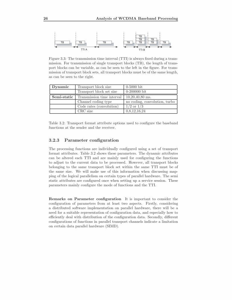
The system’s input data rate is determined by the transmission time inter-val (TTI), see Figure 3.3 and the size and number of transport blocks carryingpayload data. The output must be produced with respect to the given radioframe rate (10 ms in WCDMA), at which information is transmitted over theair. Services such as voice transmissions naturally put requirements on compu-tation end-to-end latencies for user comfort. Furthermore, since re-transmissionrequests are handled by higher layers, there is naturally also a requirement onend-to-end computation latency, in order to meet a certain quality-of-service(effective bandwidth) for varying radio conditions.
Remarks on the real-time aspects Considering mapping of different taskgraphs on parallel hardware, we see a need to explore different parallel mappingstrategies, allowing optimisation not only with respect to workload (numberof concurrent users and services) but also with respect to the given timingrequirements.
26 Analysis of WCDMA Baseband Processing
TB TB TB TB
TB
TB
TB
TTI A TTI B
TB
TB TB
Figure 3.3: The transmission time interval (TTI) is always fixed during a trans-mission. For transmission of single transport blocks (TB), the length of trans-port blocks can be variable, as can be seen to the left in the figure. For trans-mission of transport block sets, all transport blocks must be of the same length,as can be seen to the right.
Dynamic Transport block size 0-5000 bitTransport block set size 0-200000 bit
Semi-static Transmission time interval 10,20,40,80 ms.Channel coding type no coding, convolution, turboCode rates (convolution) 1/2 or 1/3CRC size 0,8,12,16,24
Table 3.2: Transport format attribute options used to configure the basebandfunctions at the sender and the receiver.
3.2.3 Parameter configuration
The processing functions are individually configured using a set of transportformat attributes. Table 3.2 shows these parameters. The dynamic attributescan be altered each TTI and are mainly used for configuring the functionsto adjust to the current data to be processed. However, all transport blocksbelonging to the same transport block set within the same TTI must be ofthe same size. We will make use of this information when discussing map-ping of the logical parallelism on certain types of parallel hardware. The semistatic attributes are configured once when setting up a service session. Theseparameters mainly configure the mode of functions and the TTI.
Remarks on Parameter configuration It is important to consider theconfiguration of parameters from at least two aspects. Firstly, consideringa distributed software implementation on parallel hardware, there will be aneed for a suitable representation of configuration data, and especially how toefficiently deal with distribution of the configuration data. Secondly, differentconfigurations of functions in parallel transport channels indicate a limitationon certain data parallel hardware (SIMD).

3.2 Downlink processing analysis 27
3.2.4 Function level parallelism
When studying the abstract task graph for the downlink, as was shown inFigure 3.2, two types of coarse-grained parallelism are naturally exposed: taskparallelism and pipeline parallelism. All data dependencies between functionsare of the producer consumer type. The channel multiplexing function (nodef8 in Figure 3.2) constitutes the first logical point of synchronisation in thedownlink task graph. Before the multiplexing function, each branch of thegraph (nodes f1 to f7) can be computed in a task parallel way, and the functionswithin each branch can be computed in a pipeline parallel way. The functionsprocessing the composite transport channel (nodes f8 - f10) are pipeline parallel.After physical channel mapping (node f10), the functions (nodes f11-f12) canbe mapped task parallel (if several physical channels are used) and pipelineparallel within each physical channel flow.
Remarks on task and pipeline parallelism On an abstract level, bothpotential task and pipeline parallelism are naturally exposed. To further de-termine potential data parallel mappings of the downlink task graph, it isnecessary also to analyse intra-function data dependencies.
3.2.5 Intra function characteristics
In our analysis we mainly consider logical parallelism exposed in the specifi-cation of the standard. To examine potential intra algorithm parallelism, weneed to analyse the computation characteristics of the standardised processingfunctions. For a more detailed analysis of the functions, the reader is referredto [Paper B]. Here we give a short summary of the characteristics.
Data dependencies The data streaming through the functions have theform of logically serial streams of binary information symbols. The functionsspecified for the downlink functions are therefore, to a large extent, performingbit serial computations. This means that there is in general no obvious fine-grained data parallelism exposed within the algorithms. However, most of thefunctions allow bit parallel mapping and computation of the data using wordlength data types. None of the symbol rate functions has data dependenciesbetween iterations, i.e. between the processing of consecutive TTIs. Thismeans that most of the task parallel functions in the downlink computationgraph potentially also, from a logical point of view, are data parallel.
Instruction level computations The computations on the data are pri-marily of a logical nature. The functions performing different kinds of datacoding, such as CRC, convolution and turbo coding, are dominated by logicalarithmetic and shift operations. Computing such functions bit serially using bit

28 Analysis of WCDMA Baseband Processing
parallel hardware is not an efficient usage of the hardware. Therefore, softwareimplemented solution of such algorithms typically make use of pre-calculatedlook-up tables whenever possible. Bit serial calculations are thus transformedto bit parallel masking and memory reads and writes. Other functions mainlyreshape the block representations of the data streams, for example the blockconcatenation and the segmentation functions. Further, another category isthe interleaving and rate matching functions, where data are either scrambledor modified on a bit level basis.
Remarks about intra function characteristics We have studied the down-link computation graph from a logical point of view, given by the 3GPP speci-fications. We conclude that logical parallelism is dominates a on function level.On the intra function level, performance gain is related more to an accelerationof computations. However, a thorough analysis of opportunities for instructionparallel computations requires implementation studies of the complete taskgraph.
3.2.6 3G service use cases
We selected two service use cases (given by the 3GPP standard) that havedifferent processing requirements on the baseband: one service configurationfor voice transmission and the other for arbitrarily high bit rate data transmis-sions. These use cases are used to analyse the processing characteristics of thedownlink functions.
Adaptive Multi Rate voice transmission Adaptive multi rate (AMR) isthe technique for the coding and decoding of dynamic rate voice data includedin the UMTS2. This technique allows dynamic alternations of the bit ratefor voice transmissions during the service session. The output of the AMRencoder is arranged in three classes of bit streams (A,B and C), depending onhow important specific bits are for quality. The A bits are the most importantand the C bits are the least important. In this use case, each of the three bitstream classes is mapped on its own dedicated user transport channel. Theoutput stream is mapped on a single physical channel.
High bit rate data transmission The 3GPP standard specifies a set ofuser equipment (UE) classes with different radio access capabilities3. Thesecapability classes define the data rates and services that must be supported fora UE of a certain class. We used the requirements for the highest capability
2Technical Specification Group Radio Access Network; Services provided the physicallayer, TS 25.302 (Release 5), www.3gpp.org
3Technical Specification Group Radio Access Network; UE Radio Access capabilities, TS25.306 (Release 5), www.3gpp.org

3.2 Downlink processing analysis 29
class supporting bit rates up to 2048 kbps4. In this use case, the input ismapped on 16 user transport channels (maximum in this UE class) and theoutput is mapped on 3 (maximum) physical channels.
3.2.7 Mapping study of the use cases
In [Paper B] we discuss mapping of the service use-cases on different typesof common parallel hardware. We studied how the services are mapped ontransport channels and what the required parameter configurations are forthe two use cases. Function by function, we reason about possibilities andcomplications for exploiting hardware supported SIMD and MIMD processingwhen mapping the downlink task graphs for each service.
SIMD mapping One possible mapping option we have studied is to logi-cally group multiple transport channels (which are logically task parallel) tobe computed using data parallel hardware. Thus we use one single instructionstream for processing n transport channels, where the user data are partitioned,mapped and computed on an n-words wide SIMD unit.
Efficient SIMD processing of multiple user channels requires that the chan-nels are uniformly configured and that the transport blocks are of equal size.For the AMR use case, this is unfortunately not the case. The transport blocksmapped on their respective transport channels are not of equal length. Tocompute the bit streams on word length hardware, the algorithm control flownaturally becomes dependent on the length of the transport blocks (recall thatmany of the functions logically compute bit serially). In the AMR case, thealgorithm control flow becomes asymmetric. Another complication is that dif-ferent CRC polynomials and convolution coding rates are used for each of thethree channels.
For the high bit rate data service, the transport blocks are of equal size.Furthermore, the configuration parameters for all transport channels can beconfigured equally. However, SIMD mapping on a transport channel basis stillintroduces complications for this use case as well. For example, algorithmsbased on look-up table techniques need to be serialised (for example, the CRCand the coding functions).
In conclusion, SIMD parallel computation on a task/data parallel usertransport channel basis introduces many complications. However, it is an openquestion whether certain functions for certain services could be beneficially(in terms of performance gain) SIMD computed. Implementation studies on alower level will be required to answer this question.
4The later addition of HSDPA and HSUPA to the 3G standard allows higher bit-rates.

30 Analysis of WCDMA Baseband Processing
MIMD mapping A MIMD processor enables asynchronous parallel compu-tations of task, data and pipeline parallelism. The trade-off, compared to aSIMD parallel mapping, is a higher cost for parallel synchronisation and com-munication (moving the data between cores) at certain points in a program.The downlink task graph naturally constitutes a good match with MIMD hard-ware.
Considering parallel implementation of WCDMA baseband processing on aMIMD structure, there are many interesting issues related to the synchronisa-tion of parallel computations and function configuration. First of all, how dowe handle the synchronisation of functions processing different TTIs of dataand how do we handle synchronised of distribution configuration parameters?
3.3 Summary and implications
This chapter provided a summary of our analysis of the WCDMA downlinkprocessing in third generation wireless telecommunication systems [Paper B].We have discussed different types of logical parallelism exposed in the WCDMAdownlink symbol rate functions. The computations are primarily of a logicalnature rather than of an arithmetical nature, further motivating expressingcomputations on variably sized bit streams of data. We have discussed possi-bilities and complications related to application mapping on certain types ofcommon parallel hardware. Further, we find it motivated to investigate ex-pressions of computations on SIMD parallel and bit level computations. Forthis application domain, it should be possible to express computations on vari-able bit fields of data as well as data parallelism on the word length of data.Real-time applications, such as the 3G baseband, require task graph mappingstrategies with respect to non-functional properties such as computational tim-ing constraints.

Chapter 4
STREAMING MODELS
OF COMPUTATION

32 Streaming Models of Computation
This chapter introduces streaming models of computation, and we describethe synchronous dataflow model of computation in particular. We motivatethe focus on the synchronous dataflow model of computation with respect tothe baseband study discussed in Chapter 3 and with respect to the type ofmanycore architectures we are investigating. Finally, we briefly describe thework presented in [Paper C], where we provide a small modelling frameworkfor elaborating with domain specific SDF languages.
4.1 Introduction
A paradigm shift from centralised processor architectures to manycore archi-tectures will naturally also require a paradigm shift in programming models,languages, compilers and development tools. Programs must be concurrent andmalleable for highly parallel and communication exposed hardware interfaces ofmanycores. Sequential languages conventionally used in the embedded systemsindustry, such as C, and especially the supporting compiler technology, havebeen developed for sequential processor architectures exposing a global memoryspace. Especially considering non-coherent distributed memory manycores, Cdoes not offer a suitable means for expressing concurrency and other knowledgethat is important for such a machine target. Important parallel informationpresent in the applications many times must be pruned and it is often notpossible to automatically recover such knowledge.
The conventional way of describing concurrency in C programs is to usethreads, which are sequential processes logically sharing memory. Relying onthreads as a concurrent programming model for code generation to manycoreprocessors is a bad approach for at least two reasons: 1) threads provide anillusion of a shared memory space, which becomes very complex and expensiveto resolve when mapped to a distributed memory processor and 2) threads arehighly non-deterministic in their nature [Lee, 2006]). A reliable and predictableimplementation using threads is relying on programming style and well-definedthread overlay mechanisms, such as semaphores, locks, barriers etc. For au-tomatised mapping to a manycore target, such a source constitutes a state-space that is highly complex to analyse (perhaps many times even impossible),in order to realistically predict its runtime behaviour.
4.1.1 Domain specific programming solutions
We argue that domain specific development methods and tools will be neededto achieve development efficiency for manycore technology. The structure ofcomputations and processing requirements is often quite different for differentapplications.
As was discussed with one concrete example in Chapter 3, applications inthe signal processing domain typically contain a high degree of parallelism and
4.1 Introduction 33
predictable data dependencies, which together form logical function flows interms of directed graphs. The task of finding an optimal mapping of taskgraphs on a parallel processor has long been known to be an NP Hard problem[El-Rewini et al., 1995]. There are known solutions for finding near-optimalmappings in linear time [Kwok and Ahmad, 1999]. However, the graph ofcourse has to be known and, in addition, it has to be suitably constructedfor the specific optimisation objectives in question. We believe that means forconstructing such task graphs, including computational constraints, must belifted up all the way to the programmer.
Since we are mainly targeting real-time applications, another issue is tim-ing analysis. It is important that the schedules of computations (tasks) arepredictable to be able to optimise programs with respect to given real-timeconstraints. Moreover, timing analysis require well defined models of tasksand their properties when executed not only to ensure determinism, but also inorder to minimise run-time overhead in terms of scheduling complexity, context-switching etc.
4.1.2 Stream processing
One of the more promising matches with the signal processing domain is var-ious forms of stream processing. The term stream has become attributed toP J Landin for his work in the early 1960s, in which he used the notion ofstreams (in the context of lambda calculus) to model loop and I/O data flows[Landin, 1964]. The stream notion was later shown to be useful for researchon computational theory in different kinds of computing systems, which aregrouped using the general term stream processing systems (SPSs).
The common definition of an SPS is an implementation of a network ofprocesses that communicates via channels. Such a system can be describedby means of a graph. The processes logically compute in parallel, taking datastreams as input and producing data streams as output. SPSs in general canbe specified and analysed using different theories of stream transformers (STs)[Stephens, 1997]. An ST is defined as an abstract system that takes a set ofn input streams and produces a set of m output streams. Mathematically, anST can be described as a function
Φ : [T → A]n → [T → A]m
where A is some data set of interest, T = N represents discrete time andn, m ≥ 1.
Dataflow constitutes one very interesting flavour of SPS, which has beena subject to research on computer architecture and modelling of concurrentsoftware for more than 30 years. In dataflow, computations are either data

34 Streaming Models of Computation
driven, i.e. the processes are computing when input data is available, or de-mand driven, where processes actively request input data when they wish tofire. Much attention in the past years of research has been paid to differenttechniques for mapping and computing dataflow graphs on parallel hardware.A good overview of the advances in the research in this area can be found in[Najjar et al., 1999]. The vertices (processes) in a dataflow graph are calledactors1 [Agha, 1986], and these perform the computations. The edges im-plement FIFO buffers representing the data paths (channels) by which actorscommunicate. Communication via the channels is the only way an actor caninfluence the computation of another actor. The firing (computation) of anactor is locally controlled; an actor fires when the required input is available,and many actors may fire simultaneously. Thus, dataflow graphs are naturallyconcurrent. Actors can be of variable granularity, and hierarchical composi-tions of actors can be constructed. This also means that an actor can verywell be another dataflow graph. This is possible by treating not only actors ascompositional components but also the network [Eker et al., 2003].
4.2 Synchronous dataflow
One special case of dataflow is synchronous dataflow (SDF), developed by Leeand Messerschmitt in the middle of the 1980s [Lee and Messerschmitt, 1987].In SDF, the number of tokens produced and consumed by an actor when itfires is specified a priori for each input and output channel. A token is anabstraction for the type and size of the units of data communicated throughthe channels. If an actor can be specified with input and output rates, the actoris said to be synchronous. If all actors in a dataflow graph are synchronous, itis a synchronous dataflow graph.
There are many advantages of SDF compared to conventional dataflow. Thea priori specified token consumption and production rates enable compile timescheduling of SDF graphs. This naturally means that more efficient runtimecode can be generated since no or very little run-time execution supervisionis required [Battacharyya, 1994]. Moreover, the channels in an SDF graphrequire some form of buffer implementation. Since an SDF graph is periodicallyexecuted by a static schedule, the required buffer size is predictable and thebuffers are guaranteed never to overflow. Moreover, a consistent SDF schedulecan be executed forever without deadlock. An important property is that, aslong as the integrity of the dataflow is respected, any parallel or sequentialimplementation of the dataflow specification yields the same result.
1In older literature these are sometimes more abstractly referred to as nodes, blocks orcomputation units.

4.2 Synchronous dataflow 35
a b c
d
D
2D
1 1
1 1
1
1
2
2
Figure 4.1: Simple SDF graph illustrating rate and delay specifications, as wellas the use of feed-back loops.
4.2.1 Description of SDF
We will give a more detailed description of SDF graphs based on the definitionsin [Lee and Messerschmitt, 1987]. Figure 4.1 shows a simple example of an SDFgraph consisting of four actors and four channels. Each incoming and outgoingchannel of an actor is associated with a non-negative integer that specifies thetoken consumption and production rates. We use rin to denote consumptionrate and rout to denote production rate. A channel connecting an output ofactor a to an input of actor b is denoted c(a, b).
Actor An actor is an atomic unit of computation that consumes and producesdata through a finite set, P = Pin ∪ Pout, of ports. The set Pin is inputports and the set Pout is output ports and Pin ∩ Pout = ∅. When anactor fires, it consumes rin tokens from all p ∈ Pin and, after firing, ithas produced rout tokens on all p ∈ Pout.
Channel A channel is a FIFO queue. When an actor consumes a token froman incoming channel, it is removed from the channel. Similarly, when atoken is produced on a channel, it is discarded.
SDF graph An SDF graph (SDFG) is a tuple (A, C) with a finite set, A,of actors and a finite set, C ⊆ Pout × Pin, of channels. Every port isconnected to precisely one c ∈ C and every c ∈ C is connected to ports,such that the source of every c ∈ C is an output port of some actor andthe destination of every c ∈ C is an input port of some actor.
Delay Let c(ai, aj) be the channel connecting an output port of actor ai to aninput port of actor aj . If c(ai, aj) has k units of delay, it means that thenth token consumed by aj will be the (n− k)th token produced by ai onc(ai, aj).
The SDF graph in Figure 4.1 has two channels specified with a sample delay:channel c(b, b), which is a feed back channel (self loop) that has a delay of one

36 Streaming Models of Computation
unit (D), and channel c(b, d), which has a delay of two units (2D). The specifieddelay corresponds to a token offset in the buffer implementing the channel inquestion.
The repetition vector, q, for the SDF graph in Figure 4.1 is 2a2bcd (or[2211]T in vector notation). The topology of an SDF graph can be describedby means of a topology matrix Γ; each row is assigned to a uniquely numberedchannel and each column is assigned to a uniquely numbered actor. If an actori produces n tokens on channel j, the element on entry (j, i) in Γ is n (theproduction rate). If an actor k produces m tokens on channel l, the elementon entry (l, k) in Γ is −m (the consumption rate negated). An actor with aconnection to itself (i.e. a self loop) has only one entry in Γ. Its value is thenet difference between the actors’ production and consumption rates on thischannel. This net difference must obviously be zero; otherwise execution of theSDF will deadlock. For all other entries, the elements are zero.
The topology matrix for the SDF graph in Figure 4.1 can be constructedas follows. Let actors a, b, c and d be numbered 1, 2, 3, 4 and let channelsc(a, b), c(b, b), c(b, c) and c(b, d) be numbered 1, 2, 3, 4, respectively. Then, thetopology matrix for the SDF graph in Figure 4.1 is
Γ =
1 −1 0 00 0 0 01 0 −2 00 1 0 −2
(4.1)
The repetition vector, q, is calculated by solving a set of linear balanceequations. The balance equations can be written in matrix form as Γ× q = O,where O is a vector of zeros. Not all SDF graphs are computable (if assumingan SDF graph to be periodic and non-terminating). For example, not appro-priately specified production and consumption rates can lead to an inconsistentspecification of an SDF graph. The consistency property (see below) of SDFguarantees that the graph can be indefinitely repeated without deadlocks.
Consistent repetition vector A repetition vector q is said to be non-trivial,if and only if q(a) > 0 for all a ∈ A. An SDFG is consistent if it has anon-trivial repetition vector q. For each SDFG that is consistent, there isa unique smallest non-trivial repetition vector that determines the mini-mum necessary firings of each actor for periodical execution of the SDFG.
Periodic and infinite admissible schedule A periodic admissible scheduleφ is a non-empty ordered list of actors such that, if actors are fired in thesequence given by φ, the amount of data buffered by channels will remainnon-negative and bounded. Each actor must appear at least once in φ. Ifφ is infinitely repeatable, φ is a periodic and infinite admissible schedule.

4.3 StreamIt: a language implementing SDF 37
Proofs and necessary conditions on matrix Γ for finding a periodic admissibleschedule can be found in [Lee and Messerschmitt, 1987].
4.3 StreamIt: a language implementing SDF
One example of a programming language implementing the SDF model of com-putation is StreamIt [Thies et al., 2002]. The StreamIt language has beendesigned with the objective of providing a portable programming model ofstreaming data applications, such as signal processing, for communication ex-posed architectures. Unlike many other languages intended for similar proces-sor targets, StreamIt provides a single machine independent concurrent lan-guage that abstracts away both the processors and the communication [Dulleret al., 2003][Das et al., 2004][PACT, 2005][Eichenberger et al., 2005].
In StreamIt, an actor roughly corresponds to a filter. Hierarchical StreamItprograms are created using pipelines, which are container constructions per-forming no computations themselves. Parallel streams are restrictively ex-pressed using split and join constructions, offering a pre-defined and limitedset of basic join and split policies. Furthermore, StreamIt filters are limitedto having single stream input and output. Thus, StreamIt enforces a highlyregular (restricted) channel connectivity of SDF programs.
4.3.1 Limitations in StreamIt
We studied issues when StreamIt is used as the implementation language forthe WCDMA downlink processing. The single stream input and output ofactors obviously limits expressibility. This can indeed become problematic forcertain concurrent function flows with more complex (multiple) data dependen-cies. However, for implementation of the function flow in WCDMA downlink,it was shown in Section 3 that most data dependencies are of a single streamproducer consumer type. Thus, neither the single stream limitation nor therestricted set of split and join policies becomes an issue from this point of view.However, we find the single stream more limiting, when considering periodicaldistribution of baseband configuration parameters. Mixing computation datawith configuration data introduces undesired dependencies between token off-sets in a stream and in the filter code. More precisely, the programmer mustcarefully consider early in the design which part (offsets) of the stream is con-trol data and which part is computation data. If consumption or productionrates of control or data at any time during development are changed, bothcontrol and computation code might have to be revised.
The concurrent stream constructions (split and join) and the hierarchicalpipeline construction enable adjustment of the granularity of function paral-lelism when possible. However, there are no syntactical means for explicitly

38 Streaming Models of Computation
expressing fine-grained data parallelism for single instruction computations (i.e.SIMD) on vectors of data. Ritz et al. developed techniques for automatic vec-torization based the SDF rate specifications [Ritz et al., 1993]. However, webelieve that offering syntactical means for expressing computations on dataparallel types will increase programmers’ awareness of such parallelism andthereby enable different alternative implementations of data parallel filter (ac-tor) code.
Further, as concluded in the WCDMA analysis, the dominating form ofcomputations are bit level computations on serial bit streams of data. Nosyntactical means is provided to be able to express computations on variablesized bit fields.
4.4 A modelling framework for SDF languages
We implemented a modelling framework in Java for prototyping and elaborat-ing with extensions and improvements on data types, operators and streamconstructions related to the StreamIt language. The motivation for build-ing such a framework is to provide a means to easily experiment with anddemonstrate extensions to such languages. In particular, we were motivatedto elaborate with possible improvements concerning the limitations we expe-rienced in StreamIt. In [Paper C] we propose different machine independentdata types and operators, as well as extended filter constructions for dealingwith periodical filter reconfiguration.
4.4.1 The StreamBits language
In [Paper C] we further present a small prototype language, StreamBits, whichwe use to demonstrate types and operators for bit level and data parallelcomputations. Moreover, we propose the introduction of logical configura-tion streams to express distributed filter reconfiguration. We later learnedthat Solar-Lezama et al. in 2005 also presented a tool (unfortunately) namedStreamBits, which addresses bit stream computations in the StreamIt language[Solar-Lezama et al., 2005]. However, their approach was to use a sketchingtechnique (template based programming) to provide bit structural informa-tion to the compiler. Further, they did not address filter reconfiguration andfine-grained data parallelism.
Similar to StreamIt, a StreamBits program is composed using Filter andPipeline components. However, StreamBits supports dual input and outputstreams – one for data and one for configuration data. The data stream consti-tutes the stream on which a filter performs its computation. The configurationstream is used to periodically distribute reconfiguration parameters to filtersthroughout the distributed network.

4.5 Related work 39
A StreamBits Filter has three basic execution modes – init, work andconfigure. Transitions between these modes are mapped automatically atcompilation time, and the programmer only needs to define the functionalitywithin each mode. The init mode is executed once, before the first firing ofthe filter, to initialise variables and parameters, and the work mode executesthe fire code. The configure mode is a feature not supported in StreamIt.It is executed once before each execution of the work mode. The configure
mode has been implemented to support more flexible programming of periodicalfilter reconfiguration of the baseband algorithms (recall the transport formatparameters describe in Section 3). With a configure mode and a logicallyseparate configuration stream, configuration programming can be defined andmodified without any changes in the filters’ fire (work) code.
StreamBits supports the common types and arithmetic operators in StreamIt.We have also introduced types to support representation and computation onbit field data and data parallel vectors. We describe these types in [PaperC] and also briefly demonstrate the usage of the types and some of the typespecific operators with a small example.
4.5 Related work
There are several other, both recent and earlier, approaches that have beentaken for domain-specific programming of embedded systems based on stream-oriented models. A large amount of various stream processing languages hasbeen researched and developed during the past 30 years. See [Stephens, 1997]for a good survey. Well known synchronous languages are SIGNAL [Gautieret al., 1987], LUSTRE [Halbwachs et al., 1991] and SISAL [Gaudiot et al., 1997],which require inputs to be available before firing computations. ESTERELis a concurrent real-time programming language but which was designed forasynchronous dataflow systems [Berry and Gonthier, 1992].
Brook is a programming language based on C but it has been extendedwith data-parallel constructs [Buck et al., 2004]. Computations that operateon local data are described using a kernel construct. Access to memory mustbe arranged using special stream constructs, where the stream elements canbe primitive scalars, vectors or record constructs. The Brook language wasdesigned to be adoptable to a wide range of manycore and so called streamprocessors such as Imagine, Trips and Raw[Kapasi et al., 2003][Burger et al.,2004][Taylor et al., 2004]. In the work reported, it has, however, mainly beenused for experiments on programming of graphics acceleration hardware, suchas the NVIDIA GeForce 6800.
Other languages very similar to Brook are Cg [Mark et al., 2003] and theStreamC/KernelC language. The Cg language is a language specialized forgraphics hardware, which uses the concept of stream kernels but does not
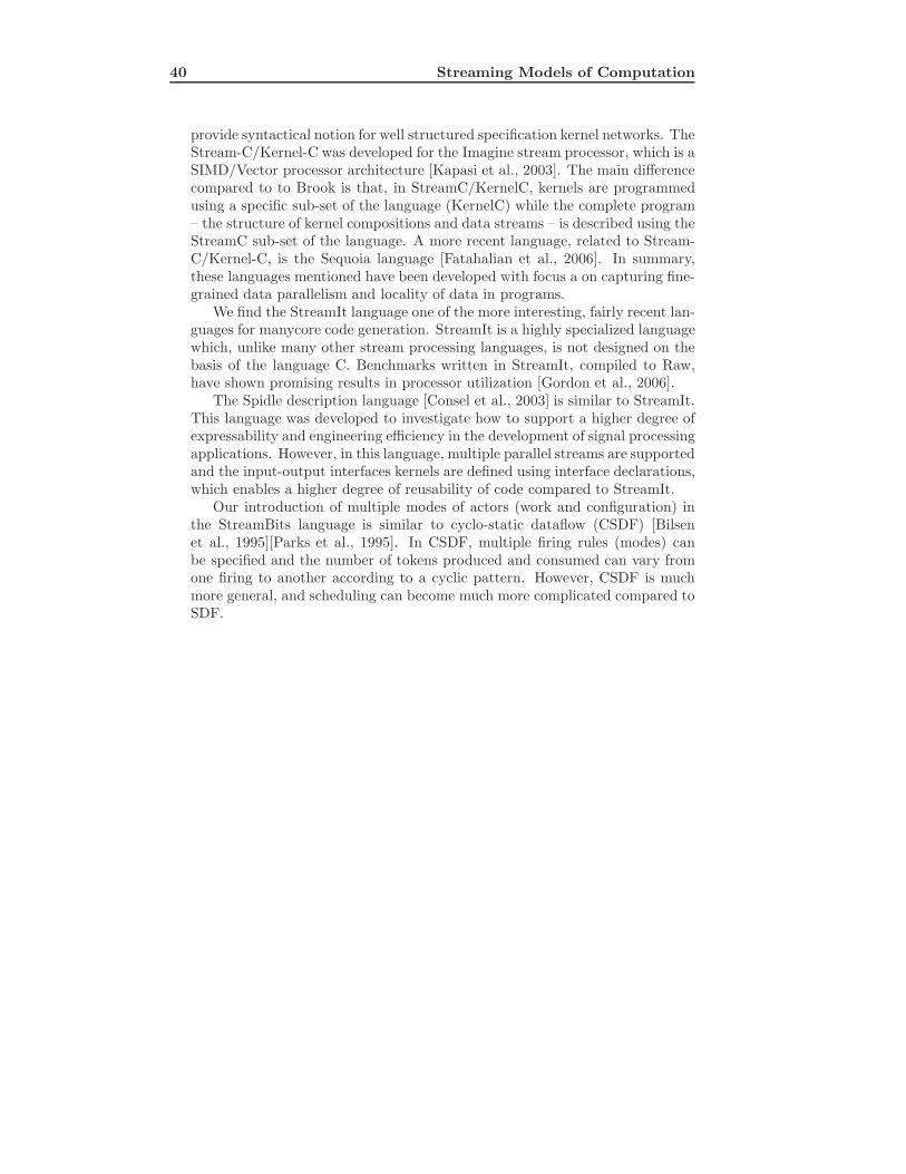
40 Streaming Models of Computation
provide syntactical notion for well structured specification kernel networks. TheStream-C/Kernel-C was developed for the Imagine stream processor, which is aSIMD/Vector processor architecture [Kapasi et al., 2003]. The main differencecompared to to Brook is that, in StreamC/KernelC, kernels are programmedusing a specific sub-set of the language (KernelC) while the complete program– the structure of kernel compositions and data streams – is described using theStreamC sub-set of the language. A more recent language, related to Stream-C/Kernel-C, is the Sequoia language [Fatahalian et al., 2006]. In summary,these languages mentioned have been developed with focus a on capturing fine-grained data parallelism and locality of data in programs.
We find the StreamIt language one of the more interesting, fairly recent lan-guages for manycore code generation. StreamIt is a highly specialized languagewhich, unlike many other stream processing languages, is not designed on thebasis of the language C. Benchmarks written in StreamIt, compiled to Raw,have shown promising results in processor utilization [Gordon et al., 2006].
The Spidle description language [Consel et al., 2003] is similar to StreamIt.This language was developed to investigate how to support a higher degree ofexpressability and engineering efficiency in the development of signal processingapplications. However, in this language, multiple parallel streams are supportedand the input-output interfaces kernels are defined using interface declarations,which enables a higher degree of reusability of code compared to StreamIt.
Our introduction of multiple modes of actors (work and configuration) inthe StreamBits language is similar to cyclo-static dataflow (CSDF) [Bilsenet al., 1995][Parks et al., 1995]. In CSDF, multiple firing rules (modes) canbe specified and the number of tokens produced and consumed can vary fromone firing to another according to a cyclic pattern. However, CSDF is muchmore general, and scheduling can become much more complicated compared toSDF.

Chapter 5
MACHINE MODEL,
INTERMEDIATE
REPRESENTATION AND
ABSTRACT
INTERPRETATION
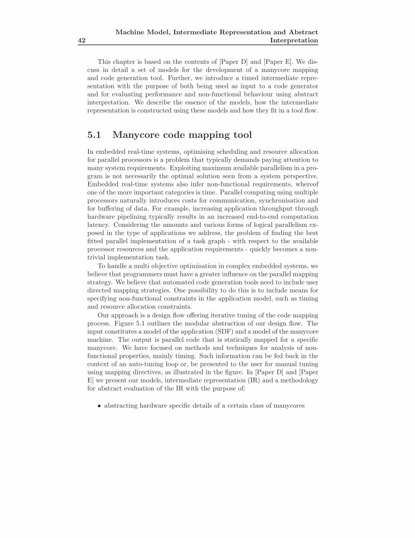
42Machine Model, Intermediate Representation and Abstract
Interpretation
This chapter is based on the contents of [Paper D] and [Paper E]. We dis-cuss in detail a set of models for the development of a manycore mappingand code generation tool. Further, we introduce a timed intermediate repre-sentation with the purpose of both being used as input to a code generatorand for evaluating performance and non-functional behaviour using abstractinterpretation. We describe the essence of the models, how the intermediaterepresentation is constructed using these models and how they fit in a tool flow.
5.1 Manycore code mapping tool
In embedded real-time systems, optimising scheduling and resource allocationfor parallel processors is a problem that typically demands paying attention tomany system requirements. Exploiting maximum available parallelism in a pro-gram is not necessarily the optimal solution seen from a system perspective.Embedded real-time systems also infer non-functional requirements, whereofone of the more important categories is time. Parallel computing using multipleprocessors naturally introduces costs for communication, synchronisation andfor buffering of data. For example, increasing application throughput throughhardware pipelining typically results in an increased end-to-end computationlatency. Considering the amounts and various forms of logical parallelism ex-posed in the type of applications we address, the problem of finding the bestfitted parallel implementation of a task graph - with respect to the availableprocessor resources and the application requirements - quickly becomes a non-trivial implementation task.
To handle a multi objective optimisation in complex embedded systems, webelieve that programmers must have a greater influence on the parallel mappingstrategy. We believe that automated code generation tools need to include userdirected mapping strategies. One possibility to do this is to include means forspecifying non-functional constraints in the application model, such as timingand resource allocation constraints.
Our approach is a design flow offering iterative tuning of the code mappingprocess. Figure 5.1 outlines the modular abstraction of our design flow. Theinput constitutes a model of the application (SDF) and a model of the manycoremachine. The output is parallel code that is statically mapped for a specificmanycore. We have focused on methods and techniques for analysis of non-functional properties, mainly timing. Such information can be fed back in thecontext of an auto-tuning loop or, be presented to the user for manual tuningusing mapping directives, as illustrated in the figure. In [Paper D] and [PaperE] we present our models, intermediate representation (IR) and a methodologyfor abstract evaluation of the IR with the purpose of:
• abstracting hardware specific details of a certain class of manycores

5.1 Manycore code mapping tool 43
Model Analysis
Dataflow Scheduling
Model Transformation
Abstract Interpretation
Code Generation
User feedback
Machine specification SDF
Manycoreconfiguration
(Timed IR)
Figure 5.1: A modular illustration of the code mapping framework.
• performing early development analysis of non-functional properties formanual or automatised map tuning of synchronous data flow graphs.
5.1.1 Target processors
An increasing amount and variety of manycore processors are commerciallyavailable. However, a big commercial breakthrough of these processors in com-puting industry has still not appeared. This is to a large extent caused by thelack of efficient development tools, established programming models and pro-cessor independent languages. We believe that dataflow models of computationwill play an important role in development tools for such processors. Our workmainly focuses on methods and techniques for dataflow code mapping to a cer-tain class of array-structured MIMD (multiple instruction multiple data) typeof manycores, as was discussed in Chapter 2. We make the following generalcategorisation (limitation) of the class of manycores we are targeting for:
Homogeneous and tightly coupled cores A homogeneous array of coreswith nearest neighbour communication simplifies construction of toolsfor code mapping. The communication network is naturally one of themore important resources that highly influence the total cost (in executiontime) for parallel execution of a task graph. Minimising communicationlatencies naturally enables exploitation of finer grained parallelism. Fur-ther, decentralizing communication between cores by means of a mesh

44Machine Model, Intermediate Representation and Abstract
Interpretation
structure increases predictability in communication timing, which is im-portant in real-time applications.
Individual instruction sequencing Many DSP algorithms contains sequen-tial computations. Naturally, some algorithms have more complex con-trol flows and/or intra algorithm data dependencies [Paper B], whichmakes them either very difficult or very costly to process spatially (i.e.instruction-level streaming). We believe that manycores offering a bal-anced mix of spatial and temporal mapping possibilities are better suitedfor software implementation of arbitrary signal processing graphs.
Distributed memory A coherent shared memory architecture simplifies theprogrammer’s task. However, such memory architectures tend not toscale well when the number of cores is growing [Barua et al., 1999]. Mostdata dependencies in DSP applications are of a producer consumer typeand happen fairly regularly in time. Non-coherent distributed memoryarchitectures (bank exposed) allow programmers and mapping tools totake advantage of locality and reduce network contention and overheadwhen accessing shared memory resources.
Software managed memory transactions Conventional hardware imple-mented caching introduces unpredictable timing and complicates real-time analysis [Muller et al., 1998]. Since the flow of functions and thedata dependencies between functions in DSP applications often follow afairly predictable pattern [Paper B], manycores with software managedtransactions on shared memory banks can be used. This reduces thecomplexity of real-time analysis on memory transactions and schedulingof network communication.
5.2 Model set
The design and construction of a tool for manycore code mapping require a setof models for abstraction of the hardware resources and the way applications arecomputed on the target hardware. The models are needed to be able to developstrategic algorithms required for transformation of the high-level program inputto a hardware configuration output. Besides serving as a resource abstractionfor the hardware, the machine model further needs to provide performancemetrics useful for estimation of dynamic computation costs.
5.2.1 Application model
Our choice of application model is the SDF. To be able to analyse the costresulting from different choices of transformation during the mapping process,and to be able to analyse the execution cost when processing a certain SDF

5.2 Model set 45
graph on manycore hardware, we need measures of execution times and re-quirements on communication and memory usage. We assume these data tohave been collected (specified by the user and/or during the model analysis,see Figure 5.1). For each actor a we assign an individual tuple
< rp, rm, Rs, Rs >
where
• rp is the worst case execution time of a, in number of operations
• rm is the maximum requirement on memory allocation of a, in numberof words
• Rr = [rr1, rr2
, . . . , rrn] is a sequence where rrn
is the consumption ratefor each input channel 1 : n of actor a
• Rs = [rs1, rs2
, . . . , rsm] is a sequence where rrm
is the production rate foreach output channel 1 : m of actor a.
We have chosen to rely on constant measures of execution times (the worstcase) in order to keep our models simple. For actors where the computations arestate or data dependent, the execution times will vary between best case andworst case. Naturally, this will affect the prediction accuracy of the executiontrace more or less depending on the current state of the program. However,our goal is not to guarantee real-time feasibility. The main goal is to provide adynamic cost model allowing us to direct map tuning of SDF graphs.
5.2.2 Machine model
The purpose of the machine model is two-fold:
1. to capture processor resources that are important for computing thecosts of computation and communication when processing a distributeddataflow graph;
2. to provide a common machine abstraction to enable tool and applicationportability.
The machine model is a pair of tuples (M, F (M)) where M is a set ofresource parameters abstracting common machine resources and F (M) is a setof abstract performance functions abstracting common basic operations of amanycore machine. To specify a particular machine, it is required to 1) givevalues to all parameters of M and 2) define the performance functions
F (M) =< tp, ts, tr, tc, tgw, tgr >
where
46Machine Model, Intermediate Representation and Abstract
Interpretation
• tp is a function evaluating the time to execute a sequence of instructions
• ts is a function evaluating the core occupancy when sending a data stream
• tr is a function evaluating the core occupancy when receiving a datastream
• tc is a function evaluating network propagation delay for a data stream
• tgw is a function evaluating the time for writing a stream to global mem-ory
• tgr is a function evaluating the time for reading a stream from globalmemory.
The performance functions F (M) are functions of the machine parametersM (see Section 2 in [Paper D]). These functions can be used to determine theexecution costs resulting from different choices of graph transformation andresource allocation. Thus, the costs are functions of both resources and theirlocations, rather than being a static cost estimate, which for example is usedin the StreamIt compiler infrastructure for clustering [Gordon et al., 2006]. InSection 5 of [Paper E] we show how these functions are defined for the Rawprocessor.
5.3 Timed configuration graphs
Portability of both tools and application code naturally requires a manycoreintermediate representation. If the goal were just to abstract away processorspecific details, such intermediate representation could very well be a fairlysimple data structure. However, since we are also interested in analysing non-functional properties for a certain mapping of a graph, there is a need also torepresent both time and the execution model. We have developed an IR whichwe call a timed configuration graph. The usage of this graph is two-fold:
1. the IR represents an SDF program after it has been transformed andmapped on the resources offered a specific manycore. We can use this IRas input to a code generator back-end, in order to generate the code foreach core, the code for communication and the mapping of memory;
2. the IR can be used to evaluate different run-time properties using abstractinterpretation. This evaluation can either be used for feed back in anauto-tuning optimisation loop or be presented to the programmer forstep-wise tuning of the mapping constraints.

5.4 Abstract interpretation of timed configuration graphs 47
5.3.1 Construction of timed configuration graphs
We target a design flow using a two step strategy as was introduced by Sarkar[Sarkar, 1989]1. In the two step strategy, the first step consists of task clusteringand the second step consists of scheduling the clusters on the processor. Thesetwo steps are performed independently of each other. With scheduling wemean core allocation and scheduling of communication. Comparisons haveshown that a two step strategy tends to produce more qualitative mappingsthan single step strategies [Kianzad and Bhattacharyya, 2006].
A timed configuration graph GAM (V, E) describes a synchronous dataflow
program A mapped on an abstract machine M (Section 4 in [Paper E]). V isthe set of vertices and E is the set of edges. There are two types of vertices:core vertices, vp, and memory vertices, vb. A core vertex represents a set ofSDF sub-graphs of A mapped on a core. Memory vertices represent buffersmapped in shared memory. The set of edges, E, represents the configurationfor the on-chip network.
When constructing a timed configuration graph, GAM (V, E), the SDF graph
A is first clustered into sub-graphs. Each SDF sub-graph is then assigned to acore in M during the scheduling step. The edges of the SDF graph that endup inside a vertex of type vp will be implemented using local memory, so theydo not appear as top level (visible) edges in GA
M . The edges of the SDF thatreach between pairs of vertices not belonging to the same SDF sub-graphs canbe mapped in two different ways:
1. as a network connection between the two cores; such a connection isrepresented by an edge;
2. as a buffer in global memory. In this case, a memory vertex is introduced.
When GAM has been completely constructed, each vp, vb ∈ V and e ∈ E has
been assigned costs (in time) for computation, communication and memoryread and writes, respectively. The costs are calculated using the parametersof M and the performance functions F (M) (Section 3 [Paper E]). These costscomprise the static part of the costs, relative to the current time and the currentstate of the system, when computing the total cost for executing an application.
5.4 Abstract interpretation of timed configura-
tion graphs
In [Paper D] we further present how we can make an abstract interpretation ofthe timed configuration graph and how an interpreter can be implemented by
1Automated clustering and cluster scheduling are not yet implemented in our tool. Thetransformation of SDF graphs to the IR is currently done by hand.
48Machine Model, Intermediate Representation and Abstract
Interpretation
very simple means on top of a dataflow process network. We have implementedsuch an interpreter in the Ptolemy modelling environment [Brooks et al., 2008].
The process network (PN) domain2 in Ptolemy is a super-set of the SDFdomain. The main difference in PN, compared to SDF, is that PN actorsfire asynchronously and channels have no a priori specified production andconsumption rates. If an actor (process) tries to perform a read operation on anempty input channel, it will block until new data are available. The PN domainimplemented in Ptolemy is a special case of Kahn process networks [Kahn,1974]. Unlike in a Kahn process network, PN channels have bounded buffercapacity, which means that a process also temporarily blocks when attemptingto perform a write to a buffer that is full [Parks, 1995]. This property makesit possible to easily model link occupancy on the network. A dataflow processnetwork model mimics the behaviour of the types of manycores we are studyingvery well.
Timed configuration graphs are implemented by means of a heterogeneousand hierarchical dataflow model. The top level is a PN model. Core vertices areimplemented using dedicated core actors, and memory vertices are implementedusing dedicated memory actors. The SDF application model, provided as inputto the tool, is transformed to a distributed SDF model embedded in the PNmodel. The inter cluster edges in the SDF graph are cut and replaced bytop level PN channels representing the inter core communication. However,apart from this temporary cut, the SDF model is still intact. We will nowbriefly summarise our implementation of timed configuration graphs and howwe make abstract interpretation [Paper D].
5.4.1 Interpretation using Process Network
There are different possible approaches for analysing the dynamic behaviourof a dataflow model. One is to let the model calculate resource and timingproperties on itself during execution of the model. Another is to generate anabstract representation of the model. We have chosen the latter alternative.The main motivation for this decision is that we are striving for an implemen-tation that does not require modification of the underlying modelling archi-tecture in Ptolemy. Our intermediate representation and abstract interpreterare added on top of the Ptolemy infrastructure, where no modification is re-quired. Although we have not made any experimental comparison, we believethe approach of interpretation on an abstract representation of the mappedSDF graph to be more beneficial in terms of modelling performance.
Program abstraction We abstract the firing for each SDF actor by meansof a sequence, S, of receive, compute and send operations:
2In Ptolemy, a model of computation is called a domain.

5.4 Abstract interpretation of timed configuration graphs 49
S = tr1, tr2
. . . trn, tp, ts1
, ts2, . . . , tsm
The abstract operations have been bound to static costs computed using themachine model M and the performance functions F (M), presented in Section5.2.
Time There is no notion of global time in a process network. Each of the toplevel vertices of GA
M (cores and memories) is an individual process. Each of thecore processes has a local clock, t. The clock, t, is stepped by means of (notequal) time segments. The length of a time segment corresponds to the staticcost bound to a certain operation in S and possibly a dynamic cost (blockingtime) when issuing send or receive operations addressed to other cores or sharedmemories.
Cores and memory A core actor implements a state machine. For eachactor that is firing, the current state is evaluated and then stored in the history.The history is a chronologically ordered list describing the state evolution fromtime t = 0.
Memory actors model competing memory transactions by the first comefirst served policy. A read or write latency is added to the current time of aread or write operation.
States For each core, we record during which segments of time computationsand communication operations were issued. For each core actor, a state listmaps to a state type ∈ StateSet, a start time, tstart, and a stop time, tstop.The state of a vertex is a tuple
state =< type, tstart, tstop >
The StateSet defines the set of possible state types:
StateSet = {receive, compute, send, receiveMem, sendMem}
The value of tstart is the start of the time segment corresponding to the cur-rently processed operation, and tstop is the end of the time segment. For allstates, time tstop corresponds to tstart + ∆, where ∆ includes the static costbound to the particular operation. For send, receive, receiveMem and send-Mem ∆ also possibly includes a dynamic cost (blocking time) while issuing theoperations.

50Machine Model, Intermediate Representation and Abstract
Interpretation
Synchronisation of clocks The timed configuration graph is synchronisedby means of discrete events. Send and receive are blocking operations. Aread operation blocks until data are available on the edge, and a write oper-ation blocks until the edge is free for writing. During a time segment, onlyone message can be sent over an edge. Synchronisation of time between com-municating actors requires two way communication. Thus, each edge in themapped SDF graph is represented by a pair of oppositely directed edges in theimplementation of GA
M .
Network propagation time Channels perform no computation. We use adelay actor to account for propagation times over edges. The delay actor addsthe edge weight (corresponding to tc ∈ F (M)), that has been assigned to eachtop level edge during the construction of GA
M
Program interpretation The core interpreter makes state transitions de-pending on the current operation, the associated static cost of the operationand whether send and receive operations block or not (the dynamic cost). Astate generating function takes timing parameters as input and returns nextstate ∈ StateTypes.
5.4.2 Modelling limitations of the IR
The use of a process network for implementation of timed configurations graphshas some limitations. In our current implementation, the network is modelledon a relatively high level, at which communication is represented using point-to-point channels. Thus, we are currently not able to model link level concur-rency and buffer capacity of the network. This was partly a design decision,because we wanted to keep the network abstraction at a high level for reasonsof modelling performance. However, this decision was also made because of theproperties of process networks, which complicate modelling of shared resources.Processes in PN execute asynchronously, driven by the availability of data. Pro-cesses connected to shared resources therefore require active time sharing tokeep the model running. These are problems that can be solved, but at theprice of a lower level of implementation of the intermediate representation.
5.5 Evaluating modelling accuracy
In [Paper E] we make an evaluation of the tool with the purpose of:
• evaluating the accuracy of the tool’s performance predictions with respectto actual performance;

5.5 Evaluating modelling accuracy 51
CORE CORE CORE CORE
CORE CORE CORE CORE
CORE CORE CORE CORE
CORE CORE CORE CORE
RAM
RAM
RAM
RAM
Figure 5.2: Overview of the Raw processor, including the Raw memory con-figuration used for our experiments. Four non-coherent shared memory banksare located on the east side ports of the chip.
• investigating whether the predictions can be used to rank different map-pings of an application with respect to latency and throughput.
In Section 3 in [Paper E] we demonstrate how we configure the machinemodel in order to model the Raw processor. Raw is a tiled, moderately parallelMIMD architecture with 16 (4 × 4) programmable tiles (cores) [Taylor et al.,2002]. The cores are tightly connected via two different types of communicationnetworks: two statically and two dynamically routed. For our experiments, wehave use a Raw set-up with four off-chip, non-coherent memory banks, seeFigure 5.2. In the rest of this chapter we briefly summarise our experimentsand the results presented in [Paper E].
5.5.1 Experimental mapping cases
For evaluation of our tool’s prediction accuracy, we experimented with differ-ent mappings of two applications: matrix multiplication and merge sort. Wechose matrix multiplication since it requires fairly large amounts of data to becommunicated over the network and since it is good for testing the modellingof communication between the cores and off-chip shared memory. The matrixmappings on Raw are illustrated in Figure 5.3.
In contrast to matrix multiplication, our implementation of the merge sortalgorithm has very low requirements on computation and communication. Themerge sort mappings on Raw are illustrated in Figure 5.4. The computationand communication load for each node in the tree increases with the depth ofthe application graph. The different mappings of matrix and merge sort arefurther described in Section 6 of [Paper E].

52Machine Model, Intermediate Representation and Abstract
Interpretation
1
3
4
2
1
3
4
2
1
3
4
2
Matrix1 Matrix2 Matrix3
Figure 5.3: Three different mappings of the 32×32 elements matrix multiplica-tion using four cores. Square symbols represent memory and circular symbolsrepresent cores.
5.5.2 Execution strategy
Our implementations are self-timed executions [Lee and Ha, 1989]. In a self-timed execution, scheduling (execution order) and core allocation are deter-mined at compile-time, while synchronisation is handled at run-time. Eachcore executes actors according to a predetermined firing schedule. A core exe-cutes the firing of an actor first when data are available.
Initially, a self-timed execution begins computing in a non-steady stateand, later, after a number of iterations, converges to a steady state schedule.All predictions and corresponding measurements are made during steady stateexecution of the dataflow graphs. Bhattacharyya et al. studied and developedtechniques for minimising synchronisation overhead in self-timed executions onmultiprocessors [Bhattacharyya et al., 1995].
5.5.3 Comparing communication costs
Communication overhead is a major factor that typically limits performancegain in a parallel implementation. Therefore we have studied the accuracy ofthe predicted performance on send and receive operations. We use ”Rawmm”to denote predicted performance (using our tool) and ”Raw” to denote the realperformance measured on Raw.
Matrix send and receive times For each of the three test mappings ofMatrix reported (see Table 1, Section 6 of [Paper E]), the predicted receive
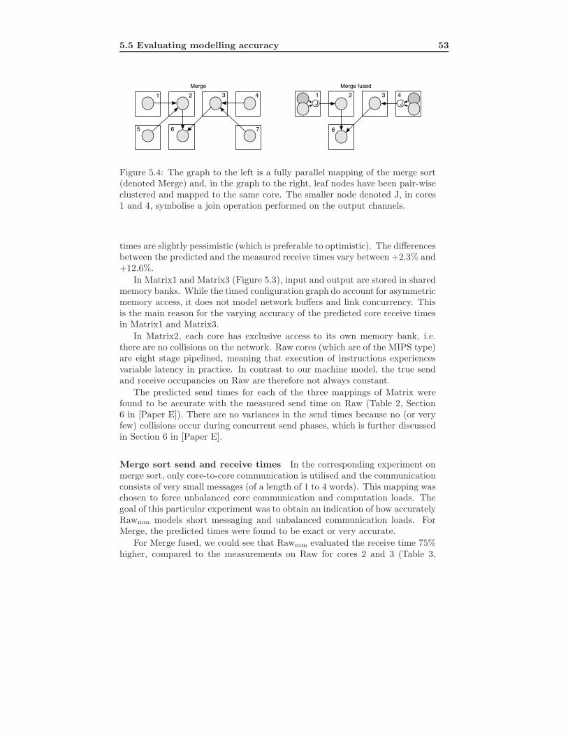
5.5 Evaluating modelling accuracy 53
1 2 3 4
6
J J
1 2 3 4
65 7
Merge Merge fused
Figure 5.4: The graph to the left is a fully parallel mapping of the merge sort(denoted Merge) and, in the graph to the right, leaf nodes have been pair-wiseclustered and mapped to the same core. The smaller node denoted J, in cores1 and 4, symbolise a join operation performed on the output channels.
times are slightly pessimistic (which is preferable to optimistic). The differencesbetween the predicted and the measured receive times vary between +2.3% and+12.6%.
In Matrix1 and Matrix3 (Figure 5.3), input and output are stored in sharedmemory banks. While the timed configuration graph do account for asymmetricmemory access, it does not model network buffers and link concurrency. Thisis the main reason for the varying accuracy of the predicted core receive timesin Matrix1 and Matrix3.
In Matrix2, each core has exclusive access to its own memory bank, i.e.there are no collisions on the network. Raw cores (which are of the MIPS type)are eight stage pipelined, meaning that execution of instructions experiencesvariable latency in practice. In contrast to our machine model, the true sendand receive occupancies on Raw are therefore not always constant.
The predicted send times for each of the three mappings of Matrix werefound to be accurate with the measured send time on Raw (Table 2, Section6 in [Paper E]). There are no variances in the send times because no (or veryfew) collisions occur during concurrent send phases, which is further discussedin Section 6 in [Paper E].
Merge sort send and receive times In the corresponding experiment onmerge sort, only core-to-core communication is utilised and the communicationconsists of very small messages (of a length of 1 to 4 words). This mapping waschosen to force unbalanced core communication and computation loads. Thegoal of this particular experiment was to obtain an indication of how accuratelyRawmm models short messaging and unbalanced communication loads. ForMerge, the predicted times were found to be exact or very accurate.
For Merge fused, we could see that Rawmm evaluated the receive time 75%higher, compared to the measurements on Raw for cores 2 and 3 (Table 3,

54Machine Model, Intermediate Representation and Abstract
Interpretation
Section 6 in [Paper E]). The reason is that the computation loads for thedownstream cores 2 and 3, after the clustering, are lower than for the upstreamstream cores (1 and 4). On Raw, each core and router entry has a buffercapacity of 5 words, allowing for several short messages to be stored on thenetwork. In contrast, Rawmm models communication pessimistically in thesense that we only allow one message at a time on a network link. Thus,communication between sender and receiver is more tightly synchronised inour model, which can potentially lead to falsely predicted blocking times, as inthis particular case.
Similarly, the predicted send times are fairly close to the measured times(the difference is 9.1% or less). The send time comparisons are shown in Table4, Section 6 in [Paper E].
5.5.4 Latency and throughput measurements
In [Paper E], we used the same mappings to compare predicted and measuredend-to-end latency and throughput. The purpose was to evaluate whether thepredictions, despite a certain deviation, could be used to correctly rank thedifferent mappings with respect to shortest latency and highest throughput.
Latency based ranking of merge sort mappings Figure 5.5 shows thepredicted latencies (in clock cycles) for Merge and Merge fused as a functionof the current iteration, compared to the measured latencies. It can be seenin the figure at which iteration each of the mappings reaches its steady stateof execution, i.e. when the latency curve levels out. For the Merge mapping,the measured latency is underestimated by a factor of 2. This is explainedby the fact that the machine model is currently not able to accurately modelthe on-chip network’s network buffer state. Thus, the difference in iterationcount between the first upstream core and the last downstream core is largerin the Raw implementation than in the modelled execution of Raw. On Raw,the end-to-end latency keeps growing until a steady state is reached. A steadystate will be reached faster in the modelled execution. To tighten the latencypredictions for certain cases of unbalanced computation loads, this experimentshows that we need to account for the network buffer capacity in the machinemodel.
For Merge fused, we can see that the latency has instead been overestimated,but is closer to the measured latency. The reason is that both the workloadand the communication load in Merge fused are better balanced than in Merge,which forces Merge fused to reach a steady state after fewer iterations.
Further, if we rank the predicted latencies of Merge and Merge fused, even ifthe predictions have varying accuracy, we still see that an optimisation decisionbased on the predictions would (for this case) correctly identify Merge fused asthe better mapping.

5.5 Evaluating modelling accuracy 55
0 2 4 6 8 10 12 14 16 180
100
200
300
400
500
600
700
800
900
1 000Merge Computation Latency
Iteration
Clo
ck c
ycle
s
Merge Rawmm
Merge RawMerge fused Raw
mm
Merge fused Raw
Figure 5.5: Comparison of predicted (Rawmm) and measured (Raw) end-to-endlatency for Merge and Merge fused.
Latency based ranking of matrix multiplication mappings Figure 5.6shows the predicted end-to-end latencies for Matrix1, Matrix2 and Matrix3,compared to the measured latencies in Raw. We can see that the three differ-ent mappings of the matrix multiplication converge to steady state at differentnumbers of iterations. Unlike in the merge sort experiment, the computationtasks distributed on the cores are naturally load balanced. The reason forthe different implementations reaching steady state at different points in timeis that the cores used in the different mappings are experience different com-munication delays due to network contention. Contention effects are a largecontributing factor to an underestimate of the latencies for Matrix1 and Ma-trix3. This can be verified by observing that the plot for Matrix2 on Rawmm
and Raw (which is a contention free mapping of the matrix multiplication) isfairly accurate compared to the predictions for Matrix1 and Matrix3. However,if we rank the predicted steady-state latencies for all mappings, we see that anoptimisation decision based on latency minimisation would also correctly sug-gest Matrix2 as the best alternative and that Matrix has shorter latency thanMatrix3.
Throughput based ranking of merge sort mappings Table 5.1 showsthe predicted and the measured throughput for Merge (within a 4.4% differ-

56Machine Model, Intermediate Representation and Abstract
Interpretation
0 2 4 6 8 10 12 14 16 1818.000
18.400
18.800
19.200
19.600
20.000
20.400
20.800
21.200
21.600
22.000Matrix Computation Latency
Iteration
Clo
ck c
ycle
s
Matrix1 Rawmm
Matrix1 RawMatrix2 Raw
mm
Matrix2 RawMatrix3 Raw
mm
Matrix3 Raw
Figure 5.6: Comparison of the modelling accuracy of the computation latencyof three different mappings of the parallel matrix multiplication.
ence) and Merge fused (within a 10% difference). The predictions are fairlyclose to the measurements on Raw for both Merge and Merge fused. We canalso see that both the predicted and the measured throughput show that Mergehas a higher throughput than Merge fused. When optimising for throughput,our predictions correctly rank Merge as the best.
Throughput based ranking of matrix multiplication mappings Table5.2 shows the comparisons of throughput for Matrix1, Matrix2 and Matrix3.Note that, unlike in all the other experiments, our model has predicted a slightlyoptimistic throughput. However, if we rank both the predicted throughput andthe measured throughput, we can also in this case see that the predictions willbe ranked in the same order as for the measured. Thus, if we use the predictionsfor throughput optimisation, our tool correctly identifies the better solution forthis example as well.
5.6 Discussion of the results
This chapter has presented an evaluation of the prediction accuracy of the tool.The communication times predicted between cores are slightly pessimistic, butwe demonstrated that, for the small set of mappings explored in the experi-

5.7 Related work 57
Application Rawmm Raw diff
Merge 119 104 +4,4%Merge fused 132 120 +10%
Table 5.1: Merge steady state periodicity (clock cycles).
Application Rawmm Raw diff
Matrix1 19249 19434 -0,9%Matrix2 19059 19143 -0,4%Matrix3 19248 19401 -0,8%
Table 5.2: Matrix steady state periodicity in (clock cycles).
ments, our tool can still correctly rank the different mappings with respect tohighest throughput or shortest latency. However, the comparisons also revealthat the predictions of end-to-end latency for unbalanced computation loadscan be quite inaccurate. This was demonstrated to be mainly dependent onthe high abstraction level used in the modelling of on-chip communication; itdoes not capture buffer state or contention effects in the network. However,this is mainly a limitation set by the current implementation of the timedconfiguration graphs.
We have at this stage only experimented with a small set of different graphlayouts (for merge sort and matrix multiplication), which are normally partsof larger application graphs. However, we believe that the slight inaccuracy(pessimism) of the predicted send of receive times is of lesser importance thancapturing buffer capacity and network contention, in terms of providing morereliable predictions for ranking task graph mappings. To capture such effects, itis necessary to include a lower level modelling abstraction of on-chip networks.Further, experiments with a more extensive set of both larger and smaller taskgraphs are needed to be able to quantify the reliability of our tool.
5.7 Related work
One of the more extensively explored problems in parallel processing is theproblem of mapping task graphs to multiprocessors. Heuristic solutions arerequired since this is known to be an NP complete problem [El-Rewini et al.,1995][Kwok and Ahmad, 1999]. In the late 1980s, Sarkar introduced the twostep mapping method, where clustering is performed in a first step indepen-dently of the second step of cluster scheduling (resource allocation), which canboth be applied at compile time [Sarkar, 1989]. A number of leading algorithms
58Machine Model, Intermediate Representation and Abstract
Interpretation
for both single step and two step clustering, with common objectives of trans-forming and mapping task graphs for multiprocessor systems, are reviewed in[Kianzad and Bhattacharyya, 2006]. A rich set of solutions is available, andthus we have not put any effort into this particular problem in our work.
The dynamic level scheduling algorithm proposed by Sih and Lee is single-step heuristic, taking inter-processor communication overhead into accountduring clustering. In a way similar to our work, Sih developed this schedulingalgorithm to be used for producing feedback to the programmer for iterativerefining of the task graph and the architecture [Sih, 1991]. However, it hasbeen demonstrated through experimental comparisons by Kianzad and Bhat-tacharyya that two step methods tend to produce more qualitative schedulesthan single step methods [Kianzad and Bhattacharyya, 2006].
Unfortunately, expanding an SDF graph to an acyclic precedence graph –which is the assumed representation for many older scheduling and mappingalgorithms – can lead to an explosion of nodes. This problem can partly be re-duced by using different clustering techniques before expanding the SDF graphto an acyclic precedence graph (APG) [Pino and Lee, 1995]. We are interestedin techniques for analysis and mapping of SDF graphs without conversion toan APG, i.e. using direct SDF representation.
The StreamIt language implements a restricted set of SDF. The StreamItcompiler implements a two step mapping (dataflow scheduling and clustering,followed by core allocation) using direct representation of SDF graphs [Gor-don et al., 2006][Taylor et al., 2002]. However, the StreamIt compiler usesa rather static cost model to determine clustering and core allocation costs.Further, neither the language nor the compiler provides any means to expressnon-functional constraints or other application specific optimisation criteria totune the parallel mapping and code generation. The dataflow scheduling, clus-tering and mapping algorithms implemented by the StreamIt compiler generateparallel mappings that make a fair trade-off between throughput and end-to-end latency. In order to improve a mapping, in terms of reducing latency orimproving throughput, programs have to be restructured.
Throughput is one important non-functional requirement in the real-timeapplications we are addressing. Ghamarian et al. provide methods for through-put using state space analysis (simulating execution of the SDF) on direct rep-resentation of multi-rate SDF graphs [Ghamarian et al., 2006]. Further, Stuijket al. developed a multiprocessor resource allocation strategy for throughputconstrained SDF graphs [Stuijk et al., 2007]. We are addressing techniquesthat allow application specific combinations of timing constraints and for howthese can be used to direct the mapping process.
Bambha et al. reviewed different intermediate representations for differ-ent objectives on optimisation and synthesis for self-timed execution of SDFprograms to multiprocessor DSP systems [Bambha et al., 2002]. They assumehomogenous representation of SDF graphs, which exposes a higher degree of

5.7 Related work 59
task parallelism based on the rate signatures. Our work is similar, but weare mainly interested in intermediate representations on multi-rate SDF and inminimising transformation between different representations during the map-ping process.
Several researchers have addressed the development of frameworks for autotuned optimisation of signal processing kernels. The FFTW system focuseson adapting the implementation of the discrete Fourier transform for differenttarget platforms using profile feed- back [Frigo and Johnson, 2005]. The SPI-RAL project focuses on automated feed- back driven optimisation of a broaderscope of signal processing kernels using machine learning techniques, startingfrom formal mathematic specifications using a symbolic language called SPL[Puschel et al., 2005]. Similar to FFTW, ATLAS is an auto tuning system forlinear algebra kernels. Commonly for these systems is that they only deal withalgorithm libraries provided by the library designer [Demmel et al., 2005].
Yotov et al. have further compared an empirical tuning engine with a model-driven tuning engine in the ATLAS system [Yotov et al., 2003]. The machineparameters used in their experiments are cache and register file sizes and thenumber of floating-point registers and floating-point multiplication units. Theyfound that model-driven optimisers can generate code with performance com-parable to code generated using empirical optimisers.
PetaBricks is a parallel language and an auto tuning compiler [Ansel et al.,2009]. In PetaBricks, it is the programmer that specifies different implemen-tations of algorithms and how they can be combined. The decision on whichalgorithm to use is determined by the PetaBricks compiler and run-time sys-tem.

60Machine Model, Intermediate Representation and Abstract
Interpretation

Chapter 6
CONCLUSIONS AND
FUTURE WORK

62 Conclusions and future work
6.1 Conclusions
The computing industry is facing a grand challenge with the entrance of many-core technology. The work presented in this thesis has addressed a few of themany issues related to development of industrial embedded high-performanceapplications using manycore technology.
The first goal of the work was to explore performance trade-offs relatedto the choice of manycore processing paradigm. In particular, we comparedarea performance trade-offs related to spatial processing on fine-grained many-cores versus temporal and spatial processing on coarse-grained manycores. Itwas estimated by calculations that a finer-grained manycore with no dedicatedcontrol logic has a clear area performance advantage over more coarse-grainedmanycores with program sequencing in each core, even if much of the dataprocessing resources must be used for program control. On the basis of typicalprocessing requirements of high-performance DSP applications, we outlined atwo level reconfigurable computer architecture based on finer-grained manycoretechnology at the lowest level.
The second goal was to investigate suitable computation models and tech-niques for programming manycores and for the development of tools for com-puter assisted mapping of signal processing task graphs. We performed an an-alytical study of parts of the baseband processing required in WCDMA radiobase stations. This study concluded that the WCDMA function flows indeedprovide a good match for implementation using stream processing models ofcomputation. We studied the WCDMA specifications with respect to differ-ent types of large-grain parallelism, the real-time aspects of such systems, andsystem reconfiguration and computation characteristics on the algorithm level.The synchronous dataflow language StreamIt was used to evaluate implemen-tation issues of the WCDMA processing in a stream processing language. Onthe basis of this evaluation, we proposed extensions to the StreamIt languageto be able to deal with instruction level data parallelism and express compu-tations on bit-serial streams and periodical reconfiguration of the distributedfilters (actors). We provided a modelling framework for practical elaborationwith languages based on the synchronous dataflow model of computation.
Finally, the third goal was to develop techniques for analysing non-functionalproperties and predicting dynamic execution costs on manycore processors.The portability of tools and application software requires a set of models toabstract application software and target processors. We presented a machinemodel that allows tool builders and application developers to specify the re-sources and the computation performance for a certain class of array structuredmanycores. Compiling source programs to an abstract manycore target furtherrequires a suitable intermediate representation. To be able to predict the dy-namic execution behaviour of a certain task graph on a certain manycore target,there is a need also to represent both the execution model and time. We have

6.2 Future work 63
proposed and developed one way to implement our intermediate representationusing a discrete event model on top of a dataflow process network. Further-more, we present techniques for predicting run-time performance by means ofabstract interpretation. It was further demonstrated, even if only for a smallset of task graphs, that the performance predictions generated were useful inranking mappings by optimisation with respect to application end-to-end la-tency and throughput.
6.2 Future work
There are several problems that we have not yet addressed and solutions weproposed that can be further refined:
Prediction accuracy It is motivated to further investigate how to includea lower, more detailed, level of network abstraction in the intermediaterepresentation. We demonstrated that it is of particular importance forprediction accuracy to include modelling of network buffers and networkcontention effects.
Automated mapping and tuning We have not dealt with automation ofthe task graph transformation and mapping process. An extensive num-ber of solutions has been reported on task graph transformation and taskgraph mapping on multiprocessors that can be used as a basis. Fur-ther work should investigate how predicted feed back can be beneficiallyused in combination with user specified mapping constraints to tune themapping process.
Heterogeneous application models The synchronous dataflow model ofcomputation has many advantages that simplify model analysis, modeltransformation and the generation of compact code. However, one trade-off for these advantages is a limited expressibility. We see a need forinvestigating the usage of heterogenous models of computation for appli-cation development and how to efficiently implement them on manycorehardware.
Dynamic resource mapping In our work, we have only dealt with the caseof static mapping of application graphs. Such a mapping can often only beused to describe smaller parts of a system or a system in a limited statespace. In industrial applications of the kind that we address, systemsmust be able to handle fast and adaptive reconfiguration of task graphs.There is a need to further investigate combined static and dynamic taskgraph mapping and resource allocation methods.

64 Bibliography

Bibliography
Agha, G. (1986). Actors: a model of concurrent computation in distributedsystems. MIT Press, Cambridge, MA, USA.
Ahlander, A. (2007). Efficient Parallel Architectures for Future Radar SignalProcessing. PhD thesis, Chalmers University of Technology.
Ansel, J., Chan, C., Wong, Y. L., Olszewski, M., Zhao, Q., Edelman, A., andAmarasinghe, S. (2009). PetaBricks: A language and compiler for algorithmicchoice. In Proc. of ACM SIGPLAN Conf. on Programming Language Designand Implementation, Dublin, Ireland.
Asanovic, K., Bodik, R., Catanzaro, B. C., Gebis, J. J., Husbands, P., Keutzer,K., Patterson, D. A., Plishker, W. L., Shalf, J., Williams, S. W., and Yelick,K. A. (2006). The landscape of parallel computing research: A view fromBerkeley. Technical Report UCB/EECS-2006-183, EECS Department, Uni-versity of California, Berkeley.
Bambha, N., Kianzad, V., Khandelia, M., and Battacharyya, S. (2002). Inter-mediate representations for design automation of multiprocessor DSP sys-tems. In Design Automation for Embedded Systems, volume 7, pages 307–323. Kluwer Academic Publishers.
Barua, R., Lee, W., Amarasinghe, S., and Agarwal, A. (1999). Maps: acompiler-managed memory system for Raw machines. ACM SIGARCH Com-puter Architecture News, 27(2):4–15.
Battacharyya, S. S. (1994). Compiling Dataflow Programs for Digital SignalProcessing. PhD thesis, University of California at Berkeley.
Baumgarte, V., May, F., Vorbach, M., and Weinhardt, M. (2001). PACT XPP- a self-reconfigurable data processing architecture. In Proc of Int’l Conf.on Engineering of Reconfigurable Systems and Algorithms, Las Vegas, NV,USA. CSREA Press.

66 Bibliography
Bengtsson, J. and Lundin, B. (2003). Reconfigurable architectures for high-performance computing. Master’s thesis, Technical report IDE0306, Halm-stad University, Halmstad, Sweden.
Berry, G. and Gonthier, G. (1992). The ESTEREL synchronous program-ming language : design, semantics, implementation. Science of ComputerProgramming, 19(19).
Bhattacharyya, S. S., Sriram, S., and Lee, E. A. (1995). Minimizing synchro-nization overhead in statically scheduled multiprocessor systems. In Proc.of the IEEE Int’l Conf. on Application Specific Array Processors, page 298,Washington, DC, USA. IEEE Computer Society.
Bilsen, G., Engels, M., Lauwereins, R., and Peperstraete, J. (1995). Cyclo-static data flow. In Proc. of the IEEE Int’l Conf. on Acoustics, Speech, andSignal Processing, volume 5, pages 3255–3258 vol.5.
Brooks, C., Lee, E. A., Liu, X., Neuendorffer, S., Zhao, Y., and Zheng, H.(2008). Heterogeneous Concurrent Modeling and Design in Java (Volume 1:Introduction to Ptolemy II). Technical Report UCB/EECS-2008-28, EECSDept., University of California, Berkeley.
Buck, I., Foley, T., Horn, D., Sugerman, J., Fatahalian, K., Houston, M.,and Hanrahan, P. (2004). Brook for GPUs: Stream computing on graphicshardware. ACM Trans. on Graphics (SIGGRAPH 2004), 23(3):777–786.
Burger, D., Keckler, S. W., McKinley, K. S., Dahlin, M., John, L. K., Lin, C.,Moore, C. R., Burril, J., McDonald, R. G., and Yoder, W. (2004). Scaling tothe end of silicon with EDGE architectures. IEEE Computer, 37(7):44–55.
Carmean, S. H. G. F. B. D. M. and Hall, J. C. (2001). Managing the impactof increasing microprocessor power consumption. Intel Technology Journal,5(1).
Consel, C., Hamdi, H., Reveillere, L., Singaravelu, L., Yu, H., and Pu, C.(2003). Spidle: A DSL approach to specifying streaming applications. InProc. of the 2nd Int’l Conf. on Generative Programming and ComponentEngineering, pages 1–17. Springer-Verlag New York, Inc.
Dally, W. J. (1990). Performance analysis of k-ary n-cube interconnectionnetworks. IEEE Trans. on Computers, 39(6):775–785.
Das, A., Mattson, P., Kapasi, U., Owens, J., , and Rixner, S. (2004). Imagineprogramming system user’s guide. cva.stanford.edu/projects/imagine.
Demmel, J., Dongarra, J., Eijkhout, V., Fuentes, E., Petitet, A., Vuduc, R.,Whaley, R., and Yelick, K. (2005). Self-adapting linear algebra algorithmsand software. Proc. of the IEEE, 93(2):293–312.

Bibliography 67
Duller, A., Panesar, G., and Towner, D. (2003). Parallel processing - thepicoChip way! In Proc. of Communicating Process Architectures, pages 125–138, Enschede, Netherlands.
Eichenberger, A. E., O’Brien, K., O’Brien, K., Wu, P., Chen, T., Oden, P. H.,Prener, D. A., Shepherd, J. C., So, B., Sura, Z., Wang, A., Zhang, T., Zhao,P., and Gschwind, M. (2005). Optimizing compiler for the CELL processor.In Proc. of the 14th Int’l Conf. on Parallel Architectures and CompilationTechniques, pages 161–172, Washington, DC, USA. IEEE Computer Society.
Eker, J., Janneck, J., Lee, E. A., Liu, J., Liu, X., Ludvig, J., Neuendorffer,S., Sachs, S. R., and Xiong, Y. (2003). Taming heterogeneity - the Ptolemyapproach. Proc. of the IEEE, Special Issue on Modeling and Design of Em-bedded Software, 91(1):127–144.
El-Rewini, H., Ali, H., and Lewis, T. (1995). Task scheduling in multiprocessingsystems. IEEE Computer, 28(12):27–37.
Fatahalian, K., Knight, T. J., Houston, M., Erez, M., Horn, D. R., Leem, L.,Park, J. Y., Ren, M., Aiken, A., Dally, W. J., and Hanrahan, P. (2006). Se-quoia: Programming the memory hierarchy. In Proc. of the 2006 ACM/IEEEConf. on Supercomputing.
Frigo, M. and Johnson, S. G. (2005). The design and implementation ofFFTW3. Proc. of the IEEE, 93(2):216–231. Special issue on “ProgramGeneration, Optimization, and Platform Adaptation”.
Gaudiot, J.-L., Bohm, W., Najjar, W., DeBoni, T., Feo, J., and Miller, P.(1997). The Sisal model of functional programming and its implementation.In Proc. of the 2nd AIZU Int’l Symp. on Parallel Algorithms / ArchitectureSynthesis, pages 112–123.
Gautier, T., Guernic, P. L., and Besnard, L. (1987). Signal: A declarative lan-guage for synchronous programming of real-time systems. Technical ReportN761, INRIA, Campus de Beaulieu, 35042 Rennes Cdex, France.
Ghamarian, A., Geilen, M., Stuijk, S., Basten, T., Theelen, B., Mousavi, M.,Moonen, A., and Bekooij, M. (2006). Throughput analysis of synchronousdata flow graphs. Proc. of Intl Conf. on Application of Concurrency toSystem Design, pages 25–36.
Gordon, M. I., Thies, W., and Amarasinghe, S. (2006). Exploiting coarse-grained task, data, and pipeline parallelism in stream programs. In Proc.of Twelfth Int’l. Conf. on Architectural Support for Programming Languagesand Operating Systems.
68 Bibliography
Halbwachs, N., Caspi, P., Raymond, P., and Pilaud, D. (1991). The syn-chronous dataflow programming language LUSTRE. In Proc. of IEEE, vol-ume 79, pages 1305–1320.
Holma, H. and Toskala, A. (2004). WCDMA for UMTS: Radio Access for ThirdGeneration Mobile Communications. J. Wiley & Sons Ltd., 3’rd edition.
Johnsson, D., Ahlander, A., and Svensson, B. (2005). Analyszing the advan-tages of run-time reconfiguration in radar signal processing. In Proc. of the17th IASTED Int’l Conf. on Parallel and Distributed Computing Systems,Phoenix, Az, USA.
Kahn, G. (1974). The semantics of a simple language for parallel programming.In IFIP Congress 74, pages 471–475, Stockholm, Sweden. North-HollandPublishing Company.
Kapasi, U. J., Rixner, S., Dally, W. J., Khailany, B., Ahn, J. H., Mattson, P.,and Owens, J. D. (2003). Programmable stream processors. IEEE Computer,36(8):54–62.
Kianzad, V. and Bhattacharyya, S. (2006). Efficient techniques for clusteringand scheduling onto embedded multiprocessors. IEEE Trans. on Paralleland Distributed Systems, 17(7):667–680.
Kwok, Y.-K. and Ahmad, I. (1999). FASTEST: A practical Low-ComplexityAlgorithm for Compile-Time Assignment of Parallel Programs to Multipro-cessors. IEEE Trans. on Parallel and Distributed Systems, 10(2):147–159.
Landin, P. J. (1964). The mechanical evaluation of expressions. The ComputerJournal, 6(4):308–320.
Lee, E. and Ha, S. (1989). Scheduling strategies for multiprocessor real-timeDSP. In Proc of the IEEE Global Telecommunications Conference, 1989, andExhibition. Communications Technology for the 1990s and Beyond, pages1279–1283 vol.2.
Lee, E. A. (2006). The problem with threads. IEEE Computer, 39(5):33–42.
Lee, E. A. and Messerschmitt, D. G. (1987). Static Scheduling of SynchronousData Flow Programs for Signal Processing. IEEE Trans. on Computers,36(1):24–35.
Mangione-Smith, W. H., Hutchings, B., Andrews, D., DeHon, A., Ebeling, C.,Hartenstein, R., Mencer, O., Morris, J., Palem, K., Prassana, V. K., andSpaanenburg, H. A. E. (1997). Seeking solutions in configurable computing.IEEE Computer, 30(12):38–43.
Bibliography 69
Mark, W. R., Steven, R., Glanville, R. S., Akeley, K., and Kilgard, M. J. (2003).Cg: A system for programming graphics hardware in a c-like language. ACMTransactions on Graphics, 22:896–907.
Moritz, C. A., Yeung, D., and Agarwal, A. (2001). SimpleFit: A frameworkfor analyzing design tradeoffs in Raw architectures. IEEE Trans. on Paralleland Distributed Systems, 12(7):730 – 742.
Muller, H., May, D., Irwin, J., and Page, D. (1998). Novel caches for predictablecomputing. Technical report, Department of Computer Science, Bristol, UK,UK.
Najjar, W. A., Lee, E. A., and Gao, G. R. (1999). Advances in the dataflowcomputational model. Parallel Computing, 25(13-14):1907–1929.
PACT (2005). Programming XPP-IIb Systems. www.pactcorp.com.
Parks, T. M. (1995). Bounded Scheduling of Process Networks. PhD thesis,EECS Department, University of California, Berkeley, Berkeley, CA, USA.
Parks, T. M., Pino, J. L., and Lee, E. A. (1995). A comparison of synchronousand cycle-static dataflow. In Proc. of the 29th Asilomar Conf. on Signals,Systems and Computers, pages 204 – 210, Washington, DC, USA. IEEEComputer Society.
Pino, J. L. and Lee, E. A. (1995). Hierarchical static scheduling of dataflowgraphs onto multiple processors. In Proc. of IEEE Int’l Conf. on Acoustics,Speech, and Signal Processing, pages 2643–2646.
Proakis, J. G. and Manolakis, D. G. (1996). Digital Signal Processing: Princi-ples, Algorithms and Applications. Prentice-Hall, Inc., Upper Saddle River,NJ, USA.
Puschel, M., Moura, J. M. F., Johnson, J., Padua, D., Veloso, M., Singer,B., Xiong, J., Franchetti, F., Gacic, A., Voronenko, Y., Chen, K., John-son, R. W., and Rizzolo, N. (2005). SPIRAL: Code generation for DSPtransforms. Proc. of the IEEE, special issue on Program Generation, Opti-mization, and Adaptation, 93(2):232– 275.
Ritz, S., Pankert, M., Zivojinovic, V., and Meyr, H. (1993). Optimum vector-ization of scalable synchronous dataflow graphs. In Proc. of Int’l Conf. onApplication-Specific Array Processors, pages 285–296.
Sarkar, V. (1989). Partitioning and Scheduling Parallel Programs for Multipro-cessors. MIT Press, Cambridge, MA, USA.

70 Bibliography
Sih, G. C. (1991). Multiprocessor Scheduling to Account for InterprocessorCommunication. PhD thesis, EECS Department, University of California,Berkeley, Berkeley, CA, USA.
Solar-Lezama, A., Rabbah, R., Bodık, R. R., and Ebcioglu, K. (2005). Pro-gramming by sketching for bit-streaming programs. In Proc. of the 2005ACM SIGPLAN Conf. on Programming language design and implementa-tion, pages 281–294, New York, NY, USA. ACM Press.
Stephens, R. (1997). A survey of stream processing. Acta Informatica,34(7):491–541.
Stuijk, S., Basten, T., Geilen, M., and Corporaal, H. (2007). Multiprocessorresource allocation for throughput-constrained synchronous dataflow graphs.In 44th ACM/IEEE Design Automation Conference, pages 777–782.
Taylor, M. B., Kim, J., Miller, J., Wentzlaff, D., Ghodrat, F., Greenwald, B.,Hoffman, H., Johnson, P., Lee, J.-W., Lee, W., Ma, A., Saraf, A., Seneski,M., Shnidman, N., Strumpen, V., Frank, M., Amarasinghe, S., and Agarwal,A. (2002). The Raw microprocessor: A computational fabric for softwarecircuits and general-purpose programs. IEEE Micro, 22(2):25–35.
Taylor, M. B., Lee, W., Miller, J., Wentzlaff, D., Bratt, I., Greenwald, B.,Hoffmann, H., Johnson, P., Kim, J., Psota, J., Saraf, A., Shnidman, N.,Strumpen, V., Frank, M., Amarasinghe, S., , and Agarwal., A. (2004). Eval-uation of the Raw microprocessor: An exposed-wire-delay architecture forILP and streams. In Proc. of Int’l. Symp. on Computer Architecture, pages2–13, Munchen, Germany.
Thies, W., Karczmarek, M., and Amarasinghe, S. (2002). StreamIt: A languagefor streaming applications. In Proc. of the 2002 Int’l Conf. on CompilerConstruction, Grenoble, France.
Wentzlaff, D. and Agarwal, A. (2004). A quantitative comparison of reconfig-urable, tiled, and conventional architectures on bit-level computation. In 12thIEEE Symp. on Field-Programmable Custom Computing Machines, pages289–290, Napa, CA.
Yotov, K., Li, X., Ren, G., Cibulskis, M., DeJong, G., Garzaran, M., Padua, D.,Pingali, K., Stodghill, P., and Wu, P. (2003). A comparison of empirical andmodel-driven optimization. In Proc. of the ACM SIGPLAN 2003 Conf. onProgramming language design and implementation, pages 63–76, New York,NY, USA. ACM.
Zhang, Z., Heiser, F., Lerzer, J., and Leuschner, H. (2003). Advanced basebandtechnology in third-generation radio base stations. Ericsson Review, (1):32–41.

List of Figures
2.1 A two level manycore hierarchy. Macro level nodes can be eitherspecialised cores, dsp or, as illustrated by the figure, a microlevel manycore structure. . . . . . . . . . . . . . . . . . . . . . 14
2.2 The figure illustrates the XPP dataflow processing array, whichis a reconfigurable MISD type of manycore. . . . . . . . . . . . 16
2.3 The figure illustrates the Raw micro processor, which is a MIMDtype of manycore array. . . . . . . . . . . . . . . . . . . . . . . 17
2.4 The block diagram to the left illustrates the implemented FFTmodule. The diagram to the right shows the amount of coresused for control flow and data flow respectively. Local memorywas needed to be used for both double buffering, in order torelax synchronisation between FFT modules when mapped ina pipelined fashion, as well as for storing pre-calculated FFTconstants . . . . . . . . . . . . . . . . . . . . . . . . . . . . . . 19
3.1 Utran. . . . . . . . . . . . . . . . . . . . . . . . . . . . . . . . . 23
3.2 Abstract task graph describing the symbol rate function flow inWCDMA downlink. The input of N user transport channelsis multiplexed (at f8 in the figure) and mapped to M physicalchannels (at f10). . . . . . . . . . . . . . . . . . . . . . . . . . . 24
3.3 The transmission time interval (TTI) is always fixed during atransmission. For transmission of single transport blocks (TB),the length of transport blocks can be variable, as can be seen tothe left in the figure. For transmission of transport block sets,all transport blocks must be of the same length, as can be seento the right. . . . . . . . . . . . . . . . . . . . . . . . . . . . . . 26
4.1 Simple SDF graph illustrating rate and delay specifications, aswell as the use of feed-back loops. . . . . . . . . . . . . . . . . . 35
5.1 A modular illustration of the code mapping framework. . . . . 43

72 List of Figures
5.2 Overview of the Raw processor, including the Raw memory con-figuration used for our experiments. Four non-coherent sharedmemory banks are located on the east side ports of the chip. . 51
5.3 Three different mappings of the 32 × 32 elements matrix mul-tiplication using four cores. Square symbols represent memoryand circular symbols represent cores. . . . . . . . . . . . . . . . 52
5.4 The graph to the left is a fully parallel mapping of the mergesort (denoted Merge) and, in the graph to the right, leaf nodeshave been pair-wise clustered and mapped to the same core.The smaller node denoted J, in cores 1 and 4, symbolise a joinoperation performed on the output channels. . . . . . . . . . . 53
5.5 Comparison of predicted (Rawmm) and measured (Raw) end-to-end latency for Merge and Merge fused. . . . . . . . . . . . . . 55
5.6 Comparison of the modelling accuracy of the computation la-tency of three different mappings of the parallel matrix multi-plication. . . . . . . . . . . . . . . . . . . . . . . . . . . . . . . 56

List of Tables
2.1 Comparison of instruction level parallelism per area for Raw withXPP and the scaled XPP. . . . . . . . . . . . . . . . . . . . . . 17
2.2 Comparison of peak performance for Raw with XPP and thescaled XPP. . . . . . . . . . . . . . . . . . . . . . . . . . . . . . 18
3.1 The table lists the types of downlink functions corresponding tothe graph in Figure 3.2. These functions are described in [PaperB]. . . . . . . . . . . . . . . . . . . . . . . . . . . . . . . . . . . 24
3.2 Transport format attribute options used to configure the base-band functions at the sender and the receiver. . . . . . . . . . . 26
5.1 Merge steady state periodicity (clock cycles). . . . . . . . . . . 575.2 Matrix steady state periodicity in (clock cycles). . . . . . . . . 57


Paper ATwo-level Reconfigurable Architecture for High-performance
signal processing
Johnsson, D., Bengtsson, J. and Svensson, B. (2004). Two-level reconfig-
urable architecture for high-performance signal processing. In Proc. of Int’lConf. on Engineering of Reconfigurable Systems and Algorithms (ERSA’04),pages 177-183, Las Vegas, USA.


Two-level Reconfigurable Architecture for High-Performance Signal Processing
Dennis Johnsson, Jerker Bengtsson, and Bertil Svensson Centre for Research on Embedded Systems, Halmstad University,Halmstad, Sweden
[email protected], [email protected], and [email protected]
Abstract
High speed signal processing is often performed as a pipeline of functions on streams or blocks of data. In order to obtain both flexibility and performance, par-allel, reconfigurable array structures are suitable for such processing. The array topology can be used both on the micro and macro-levels, i.e. both when map-ping a function on a fine-grained array structure and when mapping a set of functions on different nodes in a coarse-grained array. We outline an architecture on the macro-level as well as explore the use of an exist-ing, commercial, word level reconfigurable architec-ture on the micro-level. We implement an FFT algo-rithm in order to determine how much of the available resources are needed for controlling the computa-tions. Having no program memory and instruction sequencing available, a large fraction, 70%, of the used resources is used for controlling the computa-tions, but this is still more efficient than having stati-cally dedicated resources for control. Data can stream through the array at maximum I/O rate, while computing FFTs. The paper also shows how pipelin-ing of the FFT algorithm over a two-level reconfigur-able array of arrays can be done in various ways, depending on the application demands. Keywords: Signal processing, reconfigurable array, dataflow 1. Introduction
Many advanced signal processing applications put hard requirements on the embedded computer archi-tecture. These requirements manifest themselves as high compute requirements, limited power consump-tion, small space, low cost, etc. This means that there has to be efficient signal processing architectures. The use of dedicated hardware is common in these applica-tions, but more flexible solutions are sought for. Rather than going for the acceleration of one specific calculation one should identify domains of applica-tions and design an architecture that supports this en-tire domain. This enables building domain specific architectures rather than application specific architec-tures. Further, by the use of reconfigurable hardware it is possible to accelerate larger parts of the algorithms
than with a fixed computer architecture. In this paper we outline an architecture targeted for
multi-dimensional signal processing. It is character-ized by its two abstraction levels: the macro-level and the micro-level. In order to make efficient processing possible in a dynamic way, reconfiguration of the hardware is allowed on both levels. On the macro-level, the architecture can take advantage of the avail-able function and high-level pipeline parallelism in the applications. On the micro-level, the massive, fine-grained data parallelism allows efficient parallel and pipelined computations of algorithms such as FFTs, FIR filters, and matrix multiplications.
The micro-level is characterized by regular, highly parallel dataflow and repeated calculations. Thus, in structures for this level, it should be possible to allo-cate most of the hardware resources to the parallel data path and only minor parts to the control of the computations. Since this division of tasks is applica-tion dependent, it is interesting to study the use of architectures where the same hardware resources can be used both for data processing and for the control flow. Therefore, in this paper, we study the implemen-tation of an FFT on a reconfigurable array of arithme-tic logic units (ALUs) that can be used for either of these tasks. The goal is, of course, to use as much as possible of the available resources for the data path.
The rest of the paper is organized as follows: First we briefly describe the characteristics and demands of multi-dimensional signal processing and argue that a two-level architecture is an efficient way to achieve the required flexibility and computational power. We then discuss various micro-level structures and in par-ticular the more coarse-grained, word-level recon-figurable array architectures. We describe an imple-mentation of an FFT on one such, commercially avail-able array — the XPP. We find that, in our implemen-tation, a larger portion of the array is actually used for the flow control than for the actual butterfly opera-tions in the FFT. Still, it can be argued that the array is actually more area-efficient than a more conventional solution. The work of the control part roughly corre-sponds to the task of the program code and control logic in a microprocessor or digital signal processor. Whether the ratio between the two parts could be changed by alterations to the architecture or by more efficient mapping is still an open question.

We conclude the paper by illustrating how signal processing applications can be mapped onto the archi-tecture on the macro-level, including how an FFT computation can be mapped onto a pipeline of proces-sor arrays in order to exactly match the requirements of the application.
2. Structures for high-performance em-bedded signal processing
In high-performance embedded signal processing it
is crucial that the architecture exploits the available parallelism in an efficient way. Parallelism exists on different levels — from the macro-level function par-allelism down to the micro-level, fine-grained data parallelism. The applications considered here use multi-dimensional signal processing on streaming data. A typical example is phased array radar signal processing. In these applications, functions such as transformations and linear operations are applied on the input data volume. The functions are performed in succession, implying that a natural approach for paral-lelization of the application is to arrange a pipeline of function blocks. Since the applications considered here are multi-dimensional it also means that, for each dimension, the same sub-function is applied in parallel to all elements in that dimension. Of course, this makes it possible to execute the same function on dif-ferent dimensions in parallel. The type of functions could be matrix by vector multiplications, FIR filters, FFTs, etc. These functions themselves have inherent data parallelism. Figure 1 shows an example of a data volume in a radar application. The transformations are made on vectors along different dimensions of the volume and after each other. The size and shape of the volume can vary depending on the task performed by the radar. Moreover, radar tasks — and hence data volume shapes — may change during operation.
Samples/Range
Cha
nnel
s/B
eam
s
Pulse/Doppler
MV
M(2
)
FFT(
2)
FFT(1)
1 2 3
Figure 1. A multi-dimensional signal processing example. Functions are performed in different directions and in succession.
The applications also have real-time demands, both in terms of high throughput and in terms of latency. As a consequence of the changes in radar tasks these requirements also change. Different tasks have differ-ent requirements on throughput and latency.
An efficient architecture for embedded high speed signal processing is characterized by quantitative measures such as high compute density, both regard-ing space (operations/cm3) and power (operations/W). Other, more fuzzy, metrics could be flexibility or how much general-purpose the architecture is. The archi-tecture should offer more flexibility than those built with ASICs but it does not require the generality of a system consisting of one or more general purpose processors. The question is then what the required flexibility is for a certain domain of applications. The architecture needs to manage parallel data paths. The control of these data paths could be made in different ways. The most flexible — but least efficient — way is to have one control program for each data path, as in a microprocessor. Using one program for a group of data paths, as in a SIMD processor, or a more static mapping of the control, as found in configurable ar-chitectures, offers significant efficiency gains. These tradeoffs can be investigated by actual implementation studies on different platforms. Another vital aspect, not touched upon here, is how to develop applications for an architecture, i.e., what tools there are to support the application developer.
Demanding application domains, such as radar sig-nal processing, need highly parallel architectures. Ad-vanced radar systems may require computing 1012 arithmetic operations per second, with constraints on both space and power usage [1]. These architectures should be scaleable and support the computation of applications with highly different characteristics, e.g. different sizes and shapes of the data volume, and different demands on throughput and latency. In order to efficiently map the applications we envision map-ping of functions onto a parallel architecture where, for each function, a node or group of nodes are re-sponsible for executing the function. The nodes should then implement the calculations of the func-tions in an efficient way. The architecture should pro-vide for static mapping of the functions and the data-flow, but also provide means to quickly, during run-time, reconfigure the mapping and communication pattern to adapt to a different scenario, e.g., changing the data set shape and modifying the signal processing functions.
Embedded high-performance signal processing ap-plications often require complete systems consisting of multiple interconnected chips and even boards. It is therefore important that the architecture allows scal-ing. In order to ease the integration the same structure

should be applied repeatedly. We believe a suitable architecture is a two-level configurable architecture. The first level, the macro-level, is the target for map-ping of functions. The dataflow between nodes is con-figured on this higher level, and functions are assigned to one or a group of nodes depending on the require-ments. System configuration on the macro-level should support run-time re-allocation of nodes to functions.
An efficient architecture could be built using a mesh of nodes. A mesh architecture is scalable to lar-ger structures and is also favorable from an implemen-tation point of view. Functions could be mapped to the mesh in different ways depending on the requirements of the application. The nodes in the mesh should then, on the micro-level, execute the functions as efficiently as possible, meaning that the low-level data parallel-ism within the functions should be exploited in the most efficient way. Figure 2 illustrates this two-level approach.
Figure 2 A two-level reconfigurable architecture.
3. Micro-level structures
The primary issue regarding the design of the mi-cro-level architecture is to find a proper structure that offers a sufficient degree of flexibility to exploit the data parallelism found within the different functions. Microprocessors and DSPs offer full flexibility but do not have the performance obtainable with ASICs or configurable architectures [2]. ASICs offer the best performance regarding compute density and power consumption and are often used for high-end signal processing when DSPs fail to meet the requirements. However, ASICs are usually highly adapted for a spe-cific problem and therefore not very flexible. Another technology that has evolved and, in recent years, ma-tured to become a competitive alternative for applica-tion specific solutions is the field-programmable gate array (FPGA). FPGAs have been shown to be per-formance effective; however, fine grained FPGA cir-cuits tend to require large portions of logic to imple-ment common operations like multiplication on word length data. Major FPGA manufacturers such as Xil-
inx and Altera try to reduce this drawback by embed-ding dedicated multiplication units within the fine grained logic. Conclusively, our desire would be to find a programmable micro-level architecture that correlates well with algorithm requirements within the domain of signal processing, and which is flexible enough to exploit data parallelism within functions but also allows swift reconfigurations between functions within an application.
When choosing architecture for the micro-level there are a number of aspects that have to be ad-dressed. What are the functional requirements on the nodes? Is it possible to take advantage of the limited range of algorithms that need to be implemented? Is it possible to do without a general microprocessor and, if so, how will the control of the algorithms be imple-mented? Coarse grained reconfigurable architectures offer the possibility of implementing control flow through run-time reconfiguration, or use static con-figurations of the control flow when possible. If a reconfigurable architecture is used there are questions of how efficient the resource usage is, how the recon-figuration is done and how fast it is.
Further, the I/O bandwidth is often an issue with all signal processing architectures. The micro-level should have a balanced architecture with I/O band-width matching the compute performance. The mem-ory requirement also has to be considered. What is the proper balance between on-chip memory and comput-ing resources?
Word-level reconfigurable architectures represent one class of candidates for implementing high-performance multidimensional signal processing. The functional, control, I/O and memory issues of these architectures need to be studied in relation to the ap-plication domain. 3.1. Coarse-grained reconfigurable architec-
tures Besides programmable solutions like FPGA, which
are considered fine-grained architectures, there are many other configurable alternatives today. Many companies and academic research groups have devel-oped coarser grained, programmable processor con-cepts. The processing elements in these span a quite wide spectrum from simple ALUs [3][4] to pipelined full scale processors [5][6][7]. Two instances of these different coarse-grained paradigms are the XPP proc-essor from PACT XPP Technologies and the RAW processor developed at MIT.
The RAW processor is in principle a chip multi-processor, constituting an array of 16 full scale MIPS-like RISC processors called tiles. Characteristic for RAW is the high I/O bandwidth distributed around the

chip edges and the dynamic and static networks that tightly interconnect the processors, directly accessible through read and write operations in the register file of the processors. RAW has been implemented in a 0.15 μm process running at a worst case clock frequency up to 225 MHz. The area is reported to be 256mm2 [7]. The RAW processor with its 16 tiles has a maxi-mum peak performance of 3.6 GOPS. Large portions of a RAW tile constitute instruction fetch and decode units, a floating point unit and units for packet ori-ented interconnection routing.
The XPP, on the other hand, constitutes a 2D array of word oriented, single instruction-depth processing elements. The processing elements in the XPP are fixed-point ALU units without instruction or data memory. This means that instructions are statically mapped to processing elements and all control func-tions must be implemented using these. The instruc-tion sequencing as done in a microprocessor must be performed by mapping instructions statically to the XPP array and/or using dynamic reconfiguration of the array. Unlike RAW, which have multiple, full-fledged packet routed interconnection networks, XPP ALUs are connected via statically switched networks.
The XPP core has been implemented in a 0.13 μm process running at 64 MHz and the area requirement was reported to be 32 mm2. This roughly corresponds to a peak performance of 4.1 GOPS for the 64 ALU XPP array [8]. We are not aiming at comparing the two specific architectures. Rather, we see them as ex-amples of two architecture classes: one chip multi-processor with dedicated control and program se-quencing circuitry (RAW), the other one an ALU ar-ray (XPP) with resources only for pure dataflow proc-essing. In the latter case, some of the processing re-sources need to be used for control, and we are inter-ested to see how large portion is needed.
It is probably easier to come close to the peak per-formance in the chip multiprocessor. On the other hand, the peak performance is much higher in the ALU array. Therefore we are interested in the process-ing efficiency of the XPP array and use RAW as a reference. To make the comparison we need to nor-malize the two architectures, which we do by estimat-ing the area of the XPP array in the same process as RAW. When normalizing the area of the XPP to the 0.15 μm process used for the RAW implementation, one XPP array would be about 42mm2, which means that an XPP array occupies about 17 % (42/256) of the RAW area. Thus, 6 XPP arrays could be fitted on the same area as one RAW array. When calculating peak performance we assume the same clock frequencies as reported for XPP and RAW, this corresponds to a peak processing performance of 24.5GOPS (6 arrays at 4 GOPS) for XPP compared to 3.6 GOPS for RAW,
using the same area. Using about 15 percent of the peak performance for computations in an application would still mean that the ALU array is competitive compared to the more traditional chip multiprocessor architecture. (However, it should be noted that XPP64-A is a 24-bit architecture whilst RAW is a 32-bit architecture). Theoretically this means that up to 85% of the ALU resources, can be used to implement control functions for more complex algorithms, still the ALU array could be more effective than a chip multiprocessor, when comparing performance/area.
An obvious tradeoff is that, by making the process-ing elements simpler there is also a requirement that more ALU resources are used to implement the pro-gram control flow. Since the XPP processing elements have no instruction memory, the array needs to be reconfigured if algorithms are too large to fit on the array. This means that the designer first tries to stati-cally map as large portion of the application, data and control flow, as possible. If the complete algorithm does not fit on the array it must be temporally divided and the array is reconfigured during runtime when executing the algorithm. Even if ALU arrays offer a lot of parallelism, there is a great challenge to effi-ciently make use of it.
4. Implementation study
We have chosen to study the XPP architecture as a candidate for micro-level reconfigurability in our out-lined architecture as shown in Figure 2. In the imple-mentation study we address the control of the compu-tations implemented on this coarse-grained recon-figurable architecture. On this type of reconfigurable array architecture both computations and control func-tions have to be implemented using reconfigurable elements and communication paths. Therefore, it is interesting to see the relation between how much of the resources are used for computations and how much are used for control. 4.1. The XPP Architecture
The “extreme processing platform”, XPP, architec-ture from PACT XPP Technologies, represents a word-level reconfigurable architecture. A recent im-plementation of this architecture, the XPP64-A, oper-ates on 24-bit data.
The architecture consists of a number of parallel processing array elements labeled PAEs. There are in turn two types of PAEs, arithmetic and memory, la-beled ALU-PAE and RAM-PAE respectively. The PAEs are arranged in an array with both ALU-PAEs and RAM-PAEs, as illustrated in Figure 3. The XPP64-A has an 8x10 array, where the first and the

last columns are RAM-PAEs. Four I/O element ob-jects are connected to each of the four corners of the array. The I/O can be configured to read simple streaming input as well as to access an external mem-ory.
I/O I/O
I/OI/O
ALU
RAM
Configuration Manager
Figure 3 The XPP architecture. The highlighted areas show an ALU-PAE and a RAM-PAE includ-ing the vertical routing resources.
The array elements can be configured to execute
their operations when triggered by an event signal indicating that new data is available at the input ports. A new output can be produced every clock cycle and the result constitutes a data output and an event signal indicating that data is ready on the output port.
The ALU-PAE comprises a data path, with two in-puts and two outputs, and two vertical routing re-sources. The vertical routing resources can also per-form some arithmetic and control operations. One of the two is used for forward routing and the other for backward routing. The forward routing resource, la-beled FREG, is, besides for routing, also used for con-trol operations such as merging or swapping two data streams. The backward routing resource, BREG, can be used both for routing and for some simple arithme-tic operation between the two inputs. There are also additional routing resources for event signals which can be used to control PAE execution. The RAM-PAE is exactly the same as the ALU-PAE except that the data path is exchanged by a static RAM. The RAM-PAE can be configured to act either as a dual-ported memory or as a FIFO.
The design flow for the XPP technology constitutes using either a vectorizing C-compiler or direct pro-gramming in the native mapping language (NML), which is the XPP-ISA assembly language.
4.2. Implementation of the FFT algorithm
FFT is one important class of the algorithms often used in signal processing applications. Some of the most common FFT algorithms are the well known
Radix FFT algorithms where the algorithm complexity in computing the Fourier transformation can be re-duced from N2 to N log N [8]. By inspecting the char-acteristic Radix-2 pattern, which is illustrated in Figure 4, it is easily seen that the algorithm can be divided into logR N consecutive stages, where N is the number of samples to be processed and R is the radix of the FFT. The data in each stage is being processed and rearranged according to the characteristic radix pattern, often referred to as bit reversed order, while it is propagated through the algorithm. The basic com-putation performed at each stage is called a butterfly. As can be seen in Figure 4, the complex sample b is multiplied with a complex phase shift constant WN. The output pair (A,B) is then formed by adding and subtracting the complex sample a with bWN. In total, N/R butterflies have to be computed in each FFT stage. The FFT was chosen for the implementation study since the radix pattern requires fairly complex control functionality.
Stage1 Stage2 Stage3 Stage4WN
A = a+bWN
B = a- bWN
a
b
Figure 4 A 16-point Radix-2 Decimation In Time FFT communication pattern is shown to the left and a butterfly computation to the right.
We have used available development tools for the XPP reconfigurable architecture to implement and simulate a pipelined Radix-2 FFT. Figure 5 shows the functional schematic of an FFT module that can be configured to compute one or several butterfly stages. In this case, we use a double buffering technique be-tween two consecutive stages in the FFT so that an entire sample sequence can be read and written in par-allel without conflicts in the address space.
PrecalculatedFFT Constants
In
Out
Write
ReadButterfly
Addressgenerator
Bitreverse
fromstageN-1
tostageN+1
Sync buffer
Figure 5 Double buffered FFT stage.
Radix-2 address calculation is performed when reading the data from the buffer and streaming it to the butterfly. In order to prevent the input and output streams from accessing the same address range con-

currently, the write and read address streams have to be synchronized before the address counting is re-started after each butterfly stage. The phase shift con-stants that are multiplied with the input in the butterfly computation are precalculated and stored internally using RAM-PAEs. After the data has been streamed and processed through the butterfly it is being passed on to the consecutive stage. The RAM-PAEs can be configured to form one or several larger RAM banks dependent on the required size. We are using two separate I/O channels to stream data into the array, since we are using separate words for the real and the imaginary parts of the complex valued input. There-fore two double buffers are used to store the real and imaginary data and two memory banks to store the real and imaginary parts of the FFT constants. Figure 6 shows a block schematic of the implemented double buffer.
Buffer
Bitreverse CounterCounter
Sync
In Out
Wr Rd
Butterfly input a
Butterfly input bFrom stage N-1
Figure 6 Synchronized I/O buffers between two consecutive FFT stages.
The buffer address space is divided into a lower and an upper half and we use two separate counters to generate addresses for reading and writing to the buffer. The counter to the left in Figure 6 generates write addresses in consecutive order for the input stream. The counter to the right produces the read address which then is bit reversed to generate the characteristic Radix-2 address pattern. A counter can be implemented by combining several FREG and BREG instructions in a single PAE. The Radix-2 bit reversal is implemented using a combination of PAEs performing shifts and additions. When both counters have reached the end of each sequence, a synchroniza-tion signal is generated and fed back to the counters to make them reset and start over. 4.3. Radix-2 Butterfly
Figure 7 shows the data operation that is performed in the butterfly. Two samples are needed to compute the output from each of the N/2 butterflies in each stage. As could be seen in Figure 6, the sequential stream of samples are alternatingly forwarded to the a and b inputs in the butterfly through a PAE demux instruction. Since the XPP is a fixed point arithmetic architecture, the results from the arithmetic operations
have to be scaled to assure the output is kept within the used integer range. After the data has propagated through the butterfly, the resulting A and B samples are merged into a serial stream and then fed through the I/O channels to the next stage. This is imple-mented using PAE merge instructions.
A=a+bWN
B=a-bWNInput WN
Butterfly
a
b
Figure 7 Data stream through the Radix-2
The implemented FFT configuration is capable of processing a continuous stream of data with the speed of one complex-valued word length sample per clock cycle. All programming has been done using the NML language. All PAE configurations have been placed manually. This was made in order to achieve a func-tionally correct and balanced dataflow through the array.
Table 1 shows how large portion of the available reconfigurable resources that have been used for the FFT implementation. The available number of config-urable objects of each kind on the array is marked within the parentheses next to the name of each object. This is shown to the left in the table. For each class, the number of objects that have been configured for the FFT implementation is listed in the middle. The rightmost column shows the ratio, in percent, between used objects of each kind through the available objects of that kind.
Table 1. Array resource usage for the Radix-2 FFT.
Object Used Total share ALUs (64) 12 19% FREGs (80) 31 39% BREGs (80) 44 55% IOs (8) 4 50%
As can be concluded from the figures in the table, we use less than half of the available array resources, except for the BREGs. However, a portion of these BREGs are used for vertical routing of data on the array. We have not optimized the usage of routing resources which would likely be possible to do with more careful and strategic placement of the configured PAEs on the array.
A considerable part of all the arithmetic operations performed on the array are used for controlling the dataflow on the array. In Table 2 we have listed how many of the configured ALU operations in total that are used for controlling the dataflow and how many

are used in the butterfly, where the signal output is calculated. About 74 percent of the configured ALU resources are used for dataflow control and 26 percent are used for computing the butterfly outputs. A great portion of the resources used for the dataflow control is a consequence of using separate address counters and control functions for each of the I/O streams. The distribution of the figures may, at first look, be sur-prising. However, one should bear in mind that, in ordinary program code, many algorithms normally require portions of the code to do address calculations, incrementing and testing loop bound counters etc.
Table 2. Distribution of the total Arithmetic opera-tions. Functionality ALU ops Total share Dataflow control ops 34 74% Butterfly ops 12 26%
Out of the 12 ALU instructions used for the butter-fly configuration, two are used for fixed point scaling. The 34 ALU instructions implementing the dataflow control functionality are used for address counters, bit reverse and data path switching operations across the array. What proved to be difficult was the implemen-tation of the dataflow control structures while main-taining a balanced dataflow within the entire algo-rithm. Even though the XPP has automatic dataflow synchronization, it required time consuming, low-level engineering to balance the dataflow through all parts of the FFT and keep up a high throughput rate. Algorithms like the FFT that contain address calcula-tions, loop control and memory synchronization tend to require much of the resources to be spent on im-plementing the dataflow control in the algorithms. It might be possible to optimize the FFT implementation so that fewer configurable objects would be needed. However, solutions using long pipeline data paths tend to be complex to implement and balance on the XPP array. Therefore, in order to reduce complexity with synchronization and dataflow balance, we used separate flow control for each of the two I/O streams which resulted in the presented area tradeoff.
Still, referring back to the coarse area comparison between an array of ALUs and a chip multi processor, one could argue that, for the computation studied, the ALU array makes more efficient use of the silicon area. Even if the majority of the resources were used for control purposes, the performance achieved in our implementation is well beyond the peak performance of the more coarse-grained multi processor width dedicated control resources.
4.4. Macro-level mapping
The implemented FFT module could be used as a building block for FFTs of variable size. The perform-ance could be adapted for different requirements, by pipelining FFT modules using several nodes, which is illustrated in Figure 8. The highest configuration level — the macro level — constitutes a higher abstraction level for efficient mapping of pipeline parallelism within an algorithm, like the implemented FFT, or between different kinds of functions in a signal proc-essing chain, like in the earlier described radar signal processing application. Figure 9 illustrates the general situation. Different functions in the graph should be allocated to either a single node or a group of nodes depending on resource and performance requirements. The mapping onto the macro level should try to ex-ploit pipeline parallelism as well as parallelism stem-ming from multiple inputs.
FFT
Stage1
FFTStage
2
FFTStage
3
FFTStage
4
FFTStage
8
FFTStage
7
FFTStage
6
FFTStage
5
Idle Idle Idle Idle
FFTStage
1-3
FFTStage
4-6
FFTStage
7-9
FFTStage10-12
Figure 8 Pipelined FFT computations mapped onto the macro-level. To support dynamic mapping, the macro level archi-tecture needs to support reconfigurable interconnec-tion between the nodes. Further studies of how to best implement this, as well as how to control the configu-ration flow at the macro level and the control of data-flow between nodes, will be needed. These studies must be made using more and realistic applications to capture the characteristics of the application domain.
F1 F2 F3
F1 F2 F3
Input 0
Input 1
Output 0
Output 1
Figure 9 Functions that should map onto the macro-level structure.

5. Discussion and Conclusions We have outlined a two-level configurable archi-
tecture, intended for embedded high-performance sig-nal processing. The coarse-grained macro-level con-sists of nodes interconnected in a mesh. For the micro-level we believe reconfigurable hardware could be used for efficient implementation of the signal proc-essing functions.
We described an implementation mapping an FFT algorithm onto a coarse-grained reconfigurable architecture. With this implementation study we quantified the resource usage in the FFT algorithm. The main focus of the study was to find out how the architectural resources were allocated to different parts of the algorithm, in particular the amount of resources needed to feed the main computational core with data. This would roughly correspond to the program code and control logic in a microprocessor.
The implementation study shows that a consider-able part of the resources are used for implementing the control structures in the FFT implementation. By implementing these structures in parallel the data can be kept streaming through the nodes continuously at maximum I/O speed. The needed allocation of re-sources for control is not surprising since, in this ar-chitecture, there are no dedicated functional units for control purpose. Many algorithms in signal processing require less control than the FFT. It is possible to map these with good efficiency. Other algorithms will need reconfiguration of the array during run-time. This im-plies efficient reuse of hardware, but may have nega-tive impact on performance.
The FFT implementation has also been used to show different ways of mapping a pipelined algorithm onto several nodes of configurable arrays.
Further studies must be made to analyze the re-quirements on the interface to the micro-level nodes. On the macro-level the requirements on the communi-cation and configuration must be analyzed for differ-ent, realistic applications.
6. Acknowledgments This research has been financed by a grant from the Knowledge Foundation. We are also grateful to PACT XPP Technologies for making their development tools available to us.
7. References [1] W. Liu and V. Prasanna, “Utilizing the Power of High-Performance Computing”, IEEE Sig. Proc. Mag., Sept. 1998, pp. 85-100.
[2] A. DeHon, The Density Advantage of Configurable Computing, IEEE Computer, Vol. 33, No. 4, April 2000, pp 41-49. [3] Elixent, “Changing the electronic landscape”, http://www.elixent.com. [4] V. Baumgarte, F. May, M. Vorbach, and M. Weinhardt, "PACT XPP – A Self-Reconfigurable Data Processing Ar-chitecture," Int’l. Conf. on Engineering of Reconfigurable Systems and Algorithms ERSA 2001, Proc., CSREA Press, 2001. [5] R. Baines and D. Pulley, “A Total Cost Approach to Evaluating Different Reconfigurable Architectures for Baseband Processing in Wireless Receivers”, IEEE Com-munications Magazine, vol. 41,no. 1, Jan. 2003, pp. 105-113. [6] Paul Masters, “A look into QuickSilver’s ACM architec-ture”, EETimes, http://www.eetimes.com/story/OEG20020911S0070 [7] M. B. Taylor, et. al., ”The Raw Microprocessor: A Computational Fabric for Software Circuits and General Purpose Programs”, IEEE Micro, Mar/Apr 2002, pp. 25-35. [8] J. G. Proakis, D. G. Manolakis, Digital Signal Process-ing – Principles, Algorithms, and Applications, 3rd ed., Pren-tice-Hall International, UK (1996)

Paper BBaseband Processing in 3G UMTS Radio Base Stations
Bengtsson, J. (2006). Baseband Processing in 3G UMTS Radio Base Sta-
tions. Technical report IDE0629, School of Information Science, Computer
and Electrical Engineering, Halmstad University, Halmstad, Sweden, Feb.
2006.

Baseband Processing in 3G UMTS
Radio Base Stations
Technical Report IDE0629
Jerker Bengtsson
Centre for Research on Embedded Systems School of Information Science, Computer and Electrical Engineering Halmstad University Halmstad, Sweden

2

3
Abstract This report presents a study of functionality, service dataflows, computation charac-teristics and processing parameters for baseband processing in radio base stations. The study has been performed with the objective to develop a programming model that is natural and efficient to use for baseband programming and which can be efficiently compiled to parallel computing structures. In order to achieve this objective it is necessary to analyse and understand the logical architecture of the application in order to be able to define processing characteristics and thereby requirements on languages as well as on physical system architectures. Moreover, to be able to test and verify programming and mapping of functions it is necessary to have realistic but still manageable test cases.
The study is focused on the third generation partnership project (3GPP) standard specifications for 3G radio base stations. The specifications cover the complete 3G network-architecture and are quite extensive and complex. To make experiments manageable, it is necessary to abstract system functionality that is not directly relevant for the RBS baseband processing. Moreover, the standard specifications only describe the required processing functionality on an abstract logical level. In this report, the functionality of the baseband functions is explained and also described using illustrations of dataflows and abstract mapping of two 3G service cases.
The results of the study constitute a comprehensive description of the processing flow and the mapping of user data channels in 3G radio base stations – spanning data and control input from layer 2 to physical channel output from layer 1. Data dependencies between functions are illustrated with figures and it is concluded that these dependencies are of producer/consumer type. It is discussed how different functions can be mapped in MIMD and SIMD fashion with regard to the data dependencies, the data stream lengths and the control operations required to handle bit stream processing on word-length processor architectures.

4

5
Table of contents
1. Introduction............................................................................................................. 7 2. The UTRAN architecture........................................................................................ 8
2.1 Node B .................................................................................................................. 8 2.2 The UTRAN interfaces ......................................................................................... 9
3. Transport channel multiplexing in Node B............................................................. 9 4. Code spreading and processing rates .................................................................... 11 5. Service mapping.................................................................................................... 12
5.1 AMR voice.......................................................................................................... 12 5.2 High bit-rate data transmission ........................................................................... 13
6. Downlink processing functions............................................................................. 13 6.1 CRC attachment .................................................................................................. 13 6.2 Transport block concatenation and code block segmentation ............................ 16 6.3 Channel coding ................................................................................................... 17 6.4 Rate matching ..................................................................................................... 21 6.5 First Insertion of discontinuous transmission (DTX) indication bits.................. 25 6.6 First Interleaving................................................................................................. 27 6.7 Radio frame segmentation .................................................................................. 29 6.8 Transport channel (Trch) multiplexing............................................................... 31 6.9 2’nd Insertion of discontinuous transmission (DTX) indication bits.................. 32 6.10 Physical channel segmentation ......................................................................... 34 6.11 Second Interleaving .......................................................................................... 35 6.12 Physical channel mapping................................................................................. 37
7. Summary ............................................................................................................... 38 Appendix A: Glossary................................................................................................... 39 References..................................................................................................................... 40

6
7
1. Introduction This report concludes a study of functionality, dataflows as well as computation characteristics and processing parameters for baseband processing in Universal Mobile Telecommunication Standard (UMTS) radio base stations (RBS). The study is part of a research project where the objective is to investigate programming models and efficient mapping techniques for parallel and reconfigurable processing platforms. Efficient parallel mapping requires a programming model that is natural to use for application programming and which can be efficiently compiled to parallel structures. Thus, it should be possible to express parallelism and application-characteristic dataflows, which can be analysed and exploited at compile-time. Moreover, such a programming model should also be portable to different architectures. In order to achieve this objective it is required to analyse and understand the application, to be able to define requirements on a language and to be able to conduct realistic implementation experiments.
There are two main purposes with this study. First, the standard specifications for third generation (3G) networks are quite extensive and complex and quite difficult to grasp. To make experiments manageable, it is necessary to abstract system details that are not directly relevant for the RBS data processing. The second purpose is to characterise the baseband functions, the computations and the dataflows to understand what kind of operations and logical functionality that must be expressed in a programming language.
There are several 3G-enabling radio technologies, such as EDGE, CDMA 2000 (also called CDMA 2K) and WCDMA. WCDMA is an abbreviation for wideband code division multiple access and it is the radio technology chosen by the 3GPP organisation for UMTS networks [1]. Unlike earlier generations, 3G systems have been designed to support high bandwidth multimedia services and to support multiple simultaneous services, multiplexed on a single user channel [2].
In an RBS, the term downlink denotes the transmitting part of a communication link and the receiver link is called uplink. FDD is an abbreviation for Frequency Division Duplex, in which separate frequency bands are used for uplink and downlink carriers. There is also a standard for Time Division Duplex (TDD) in UMTS, but the FDD standard is the technology used in existing telecommunication systems. This study is focused on the WCDMA FDD standard and the downlink processing in an RBS. The technical specification in the study document has been compiled from release 5 of the 3GPP standard specifications [1].
This report is organized as follows. Section 2 describes the logical network architecture and how the RBS relates to the network. The RBS data input format, configuration parameters and the logical function flow for the baseband processing are presented in Section 3. In section 4, the WCDMA code spreading technique and processing rates are discussed. Section 5 discuses two service examples used to describe data- and function-flows. The technical specifications of the studied baseband functions are presented in Section 6 which is the main section of the report. We explain the purpose the functions and illustrate dataflows and mapping characteristics using the service examples from Section 5. Finally, the study is summarised in Section 7.
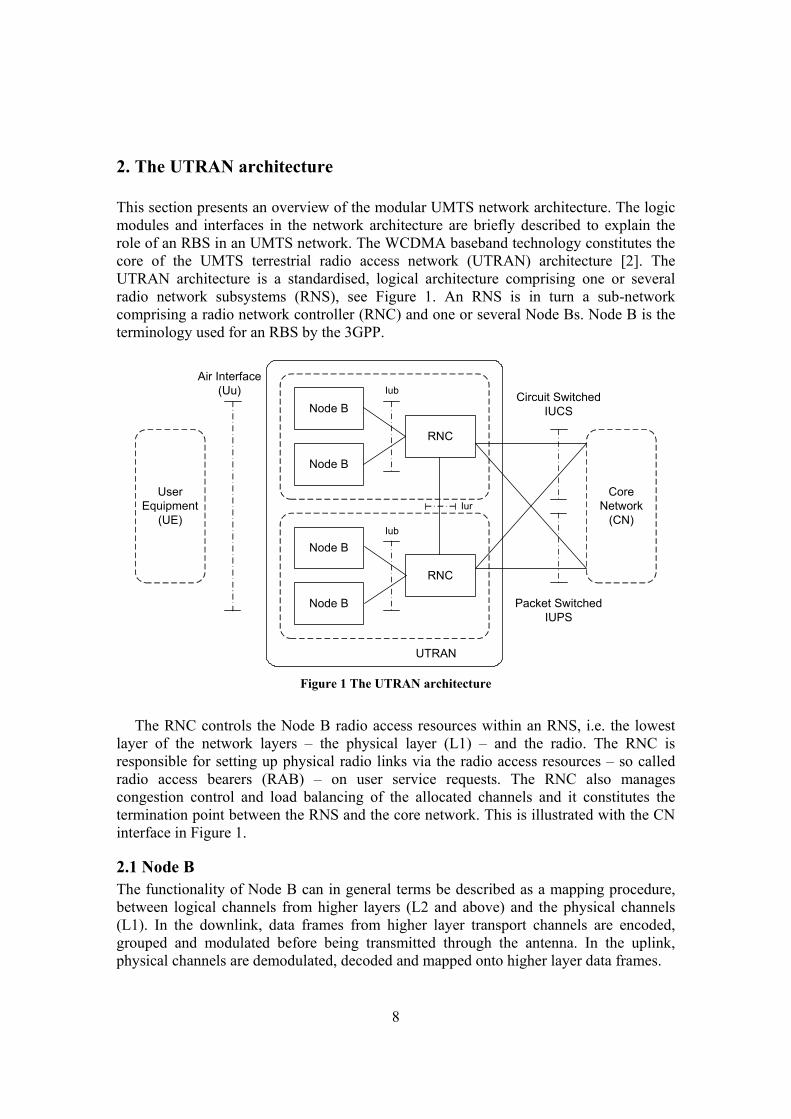
8
2. The UTRAN architecture This section presents an overview of the modular UMTS network architecture. The logic modules and interfaces in the network architecture are briefly described to explain the role of an RBS in an UMTS network. The WCDMA baseband technology constitutes the core of the UMTS terrestrial radio access network (UTRAN) architecture [2]. The UTRAN architecture is a standardised, logical architecture comprising one or several radio network subsystems (RNS), see Figure 1. An RNS is in turn a sub-network comprising a radio network controller (RNC) and one or several Node Bs. Node B is the terminology used for an RBS by the 3GPP.
Node B
Node B
RNC
Node B
Node B
RNC
CoreNetwork
(CN)
UserEquipment
(UE)
Air Interface(Uu) Circuit Switched
IUCS
Packet SwitchedIUPS
Iur
Iub
Iub
UTRAN
Figure 1 The UTRAN architecture
The RNC controls the Node B radio access resources within an RNS, i.e. the lowest
layer of the network layers – the physical layer (L1) – and the radio. The RNC is responsible for setting up physical radio links via the radio access resources – so called radio access bearers (RAB) – on user service requests. The RNC also manages congestion control and load balancing of the allocated channels and it constitutes the termination point between the RNS and the core network. This is illustrated with the CN interface in Figure 1.
2.1 Node B The functionality of Node B can in general terms be described as a mapping procedure, between logical channels from higher layers (L2 and above) and the physical channels (L1). In the downlink, data frames from higher layer transport channels are encoded, grouped and modulated before being transmitted through the antenna. In the uplink, physical channels are demodulated, decoded and mapped onto higher layer data frames.

9
The transport channels comprise channels of both dedicated and common type. The dedicated channels (DCH) are allocated for single users while the common channels are shared for several users. Several transport channels can be allocated for a single user and these are multiplexed into one coded composite transport channel (CCTRCH). Multiple transport channels can be allocated for one service and/or for multiple services running in parallel. For example, a user could be downloading e-mails in the background while speaking in the phone at the same time. In release 5 of the 3GPP standard, which is the standard release used for this report, it is only possible to allocate one CCTRCH for a single mobile user equipment (UE).
2.2 The UTRAN interfaces There are two RNC interfaces to the core network (CN) ⎯ the IUPS interface for packet switched communication and the IUCS interface for circuit switched communication. The UTRAN CN interface is designed to be logically compatible with the GSM network infrastructure.
The IUR interface is an interface for communication between RNCs of different RNSs. It is used for network relaying, or hand-over, of radio links when a mobile UE has relocated geographically in the network. The RNC that initiates a radio access link is denoted the serving RNC (SRNC). The SRNC is the owner of the link. When a mobile UE relocates to a different RNS, the RNC in the RNS to which the mobile has relocated to becomes a drift RNC (DRNC). The DRNC relays the radio link to the SRNC and no L2 processing is performed at the DRNC.
The IUB interface is the L2 to L1 interface between a Node B and the RNC. This interface is the termination point for the RBS managed resources. The Uu interface is the WCDMA air interface between Node B and mobile UEs. The physical layer processing in the RBS is encapsulated between the Iub and the Uu interfaces.
3. Transport channel multiplexing in Node B This section presents the L1 downlink logical function flow in the RBS and the frame format of input data from L2. Service payload is mapped on dedicated transport channels (DCH) and a transport block is the smallest data unit for input payload. Several transport blocks can be mapped on one transport channel and new blocks of data arrive by a deterministic time interval, Figure 2. This time interval is denoted as the transmission time interval (TTI).
TB TB TB TB TBTBTB
TBTB
TB
TTI A TTI B Figure 2 Examples of Transport block combinations

10
Transport blocks that are grouped within a TTI and belong to the same service constitute a transport block set [5]. A new transport block set is processed every TTI and the TTI is always a multiple of the 10 ms radio frame (10, 20, 40 or 80 ms). Transport blocks in different TTIs can have variable bit lengths (illustrated to the left in Figure 2), but within a transport block set, all blocks must be of equal length (illustrated to the right in Figure 2).
CRC encoding
Transport block concatenation andCodeblock segmentation
Channel Coding
Rate Matching
1'st DTX insertion
First Interleaving
Radio Frame Segmentation
Transport Channel Multiplexing
2'nd DTX insertion
Physical Channel Segmentation
Second Interleaving
Physical Channel Mapping
12
N
12
M
Symbol Rate
Chip Rate
Parallel D
CH
TRC
Hs
CC
TRC
H
Figure 3 DCH frame format. The horizontal axis is graded in bytes and the vertical axis by byte octets
Header CRC FT
CFN
TFI of first DCHSPARE
TFI of last DCHSPARE
First TB of first DCH
First TB of first DCH (contnd.) PAD
07
Payload CRC
Payload CRC (contnd.)
Last TB of first DCH
Last TB of first DCH (contnd.) PAD
First TB of last DCH
First TB of last DCH (contnd.) PAD
Last TB of last DCH
Last TB of last DCH (contnd.) PAD
Spare extension
Payload
Header
Optional
HeaderPayload
PadOptional
Figure 4 Downlink processing functions

There are two L2 frame format types for the DCHs – data frames and control frames [3]. All frames have a header field and a field for payload. The structure of a data frame can be seen in Figure 3.The baseband processing in Node B constitutes a pipelined sequence of functions, as shown in Figure 4. The figure shows N parallel DCH transport channels, which are multiplexed to form a CCTRCH, and later, depending on the bandwidth requirements, de-multiplexed on M physical channels. The processing mode of the baseband functions is configured using a set of service parameters. These processing parameters must also be set at the receiver side. Different methods can be used to configure the processing mode parameters in the receiver – TFCI based detection, blind transport format detection or guided detection [4]. The mapping examples, described later in Section 5, assume TFCI based detection.
The transport blocks transmitted within a transport channel in the same radio frame interval are combined with a transport format indicator (TFI). A transport format combination indicator (TFCI) combines the TFIs for the services that are multiplexed on a single CCTRCH. The TFCI is encoded and transmitted over the physical channel together with the DCHs which are multiplexed to form a CCTRCH. If several DCHs are used, only one TFCI is sent with one of the DCHs. At the receiver side, the TFCI can be decoded and the function parameters are then configured so that the data frames can be processed correctly.
The TFI has two parts – a dynamic part and a semi-static part. The dynamic parameters can be altered each TTI, while the semi-static are configured once when a service is set up. The TFI parameters are listed in Table 1 below.
Table 1 Transport Format Attribute options
Dynamic Part
Transport Block Size
0 to 5000 bit
Transport Block Set Size
0 to 200000 bit
Semi- Static Part
Transmission Time Interval
10, 20, 40, 80 ms
Channel Coding Type
No coding, Convolution coding,
Turbo coding
Code Rates (Convolution)
1/2 or 1/3
CRC size 0, 8, 12, 16, 24
4. Code spreading and processing rates The L1 processing is performed with different processing rates at different stages. These rates are categorised as symbol rate processing and chip rate processing. Symbol rate

12
corresponds to the rate of the information bits. That is, each bit processed in the physical layer corresponds to one information symbol (e.g. 1 or 0) in the payload. The WCDMA technology uses code spreading to enable transmission of multiple channels on the same frequency band. Symbols are spread using orthogonal channel codes. A channel code is a finite sequence of 1’s and 0’s, which are denoted chips, and these sequences are selected so that they are orthogonal to each other. Each symbol is spread to a sequence of chips and the processing rate is higher after this spreading, since each logical symbol now is represented by a longer chip-sequence. This rate is referred to as chip rate.
In the downlink, all baseband functions from the CRC attachment through the physical channel mapping are processed at symbol rate. The spreading operation is performed after physical channel mapping and the output after spreading are chip rate. In the uplink, parts of the RAKE1 receiver and the preceding functions are processed at chip rate. Functions proceeding to the RAKE receiver are processed at symbol rate.
The chip rate on a physical channel in UMTS is 3.84 Mchips and this rate is constant. A radio frame is transmitted during a 10 ms interval and this corresponds to a length of 38400 chips. Each radio frame is divided into 15 slots and each slot corresponds to 2560 chips. The length of the spread factor (SF) determines the rate with which symbols are mapped on the physical channels. The spread factor is always a multiple of 2 and in the downlink the SF can vary between 4 and 512. Dynamic bit rates can be allocated through configuration of the spread factor length and by using multiple channel codes.
5. Service mapping This section presents two 3G service examples which are used to reason about mapping of data streams and about processing characteristics of the baseband functions in Node B. The first example is derived on a standard service for voice transmission. The second example is a more general case for high-bit rate services. Only mapping and processing on DCH transport channels are considered and it is assumed that the required service RABs have been setup by the RNC.
5.1 AMR voice Adaptive Multi Rate (AMR) is a technique used for coding and decoding of dynamic rate speech services in UMTS [5]. The bit rate can be altered by the radio network during the service session, hence the name Adaptive Multi Rate2. There are two standard AMR codecs included in the 3GPP specification – narrowband AMR [6] [7] and wideband AMR [8]. The wideband AMR is specified in release 5 of the 3GPP technical specifications. The main difference is that the wideband AMR coder offers higher voice quality by means of an increased sample rate (16 kHz for wideband compared to 8 kHz when using narrowband).
Nine data rates between 6.60 kbps and 23.85 kbps are available in the wideband AMR standard. The narrowband AMR codec offers 8 data rates between 4.75 kbps and 12.2 kbps, where some of these codec rates are compatible with the AMR codec used for the 1 The RAKE receiver is used in the uplink to decode the channel codes 2 Current networks have been deployed with AMR that uses fixed bit-rates

13
GSM system. The radio access network can adaptively control the bit rate and for the narrowband AMR service the bit rate can be changed for each TTI.
When the AMR encoder encodes data, the bits are arranged in different classes according to how important they are for speech quality. The encoded bits are categorized into three classes - A, B and C - where A are the most important bits and C the least important. Stronger coding and CRC attachment can be applied on the class A bits separately, while the less important bits can be transmitted using less coding strength and without CRC attachment.
5.2 High bit-rate data transmission The standard specifies a set of UE classes with different radio access capabilities. These capability classes define what data rates and services that must be supported for a UE of a specific class. We have used parameters required for UEs of the highest capability class, which can handle bit rates up to 2048 kbps [9]. The maximum number of simultaneous transport channels for the 2048 kbps class is 16. It is assumed that all transport channels can be of DCH type. One CCTRCH using up to 3 physical channel codes can be received by a UE of this class. The maximum number of transport blocks within a TTI is 96 and the maximum number of bits that can be received within a 10 ms radio frame interval is 57600.
6. Downlink processing functions In this section we explain and discuss the baseband functions (shown in Figure 4) with focus on the downlink data channel processing in the RBS. We illustrate processing and mapping of services to these functions using the two cases of service transmissions that were presented in Section 5. The mapping is based on the logical specifications given by the 3GPP standard documents and test implementations that have been made for a sub set of these functions [1]. We use figure abstractions in connection to each of the described functions to abstractly reason about computations, potential parallelism and dataflow mapping. The mapping has been kept on an abstract level for each function separately and the specific services are discussed under the paragraphs AMR service and High bit-rate data service in connection to each function sub-section.
In first hand, we are interested in identifying data dependencies, potential parallelism and typical computations in order to define different function implementations which desirably should be possible express in a programming language.
6.1 CRC attachment Cyclic Redundancy Check (CRC) is a function used to detect bit errors after transmission. At the sender side, a checksum is calculated and appended to the data to be transmitted, Figure 5. In the figure, Ai represents the length of the transport block before CRC attachment and Li the length of the checksum. At reception, the checksum is recalculated and if no errors have been introduced, this checksum will match the appended checksum. The CRC checksum is calculated using polynomial division [10]. The dividend corresponds to the bits in a transport block and the divisor is a specified generator poly-nomial, known both by the sender and the receiver. This polynomial

14
division results in a rest term - the checksum. The generator polynomials used for CRC in UMTS are of length 24, 26, 12, 8 or 0 bits. The generator polynomial to be used for a specific transport channel is signalled to the physical layer from higher layers in the TFIs.
CRCTransport Block
Transport Block with CRC attached0 Ai+Li
Transport Block
0 Ai
Figure 5 A CRC checksum is appended to each transport block
The polynomial arithmetic is performed in GF(2), where GF is an abbreviation for
Galois Field and 2 represents a number field of width 2. In practice this means that addition and subtraction are performed modulo 2. (i.e. no carry is propagated) [11]. Thus, addition and subtraction can be implemented using simple XOR arithmetic. The following generator polynomials are specified for usage in the 3GPP UMTS standard GCRC24(D) = D24 + D23 + D6 + D5 + D +1 GCRC16(D) = D16 + D12 + D5 + D +1 GCRC12(D) = D12 + D11 + D3 + D2 + D +1 GCRC8(D) = D8 + D7 + D4 + D3 + D +1 In GF(2) each Di term represents a ‘1’ at position i in the binary number format and the others are ‘0’. For example, the polynomial GCRC8 corresponds to the binary number 110011011.
Transport blocks are padded with a number of zeros, as many as the length of the generator polynomial. That is, if GCRC16 is used, 16 zeros shall be appended to the transport block. After zero padding, the entire transport block (the dividend), is divided by the generator polynomial (the divisor). If there are no transport blocks on the input, no checksum is calculated. If the input transport block size is of zero length, a checksum is still calculated (all checksum bits will be zero).
AMR service The AMR bit classes are mapped using three RAB sub-flows; one transport block for each bit class, mapped on three separate DCH transport channels. CRC attachment is only applied for the class-A sub-flow using the CRC12 polynomial. Thus, one transport block per user must be processed each TTI, see Figure 6. A possibility for exploitation of SIMD parallelism is to combine AMR class A channel streams from several users. However, efficient SIMD parallelization of the CRC function for AMR services will require that the channels are computed using the same CRC polynomial. This is because that many efficient CRC algorithms require that the input must be sliced according to the polynomial length [10]. Also, it will require that all users are using the same AMR data

15
rate encoding modes to ensure that all bit streams are equal in length. Input slicing and stream alignment require control operations. These control operations must be the same for all streams to be able to SIMD vectorize efficiently.
DCH A DCH B DCH C CRC input
After CRC
42 - 81 53 - 103 0 - 60
12 0 - 6042 - 81 53 - 103 Figure 6 Transport block lengths can take 8 different discrete values within the given bounds. Each value corresponds to a certain AMR bit-rate.
High bit-rate data service Data can be mapped using multiple transport blocks distributed on several transport channels. All transport blocks within a transport channel are of equal length (n in Figure 7) and the CRC polynomial is the same for all blocks. Since there are no data dependencies between transport blocks, it is possible to SIMD vectorize several blocks within a channel.
Like in the AMR case, efficient SIMD vectorization of data from several transport channels will require that the transport block lengths and CRC polynomial are the same for these channels. Otherwise, more coarse-grained parallelism can be exploited by mapping the channel streams in a MIMD parallel fashion.
For the 2048 kbps class, at most 96 transport blocks can be mapped to 16 DCH streams, as shown in the figure. The maximum sum of bits that can be received within a TTI (all DCH:s included) is 57600 ( channelsii nnm ×× ).
DCH 1
CRC input of
After CRC0-24 bits attached
0 - n1
0-240 - n1
DCH 2
0 - n2
0 - n2
DCH 16
0 - ni
0 - ni0-24 0-24
DCH 1 DCH 2 DCH 16
mi blocks of size niwhere i is 0 - 16
channels
1
m
Figure 7 Transport blocks are mapped on 0-16 channel streams. A CRC checksum of length 0 - 24 bits is attached to each block

16
6.2 Transport block concatenation and code block segmentation Transport blocks mapped within a transport channel during the same TTI are concatenated to larger code blocks. If the resulting code block is larger than a maximum code block size, it will be segmented into several code blocks. The purpose with code block concatenation and segmentation is to build code blocks with a size that yields better coding performance of the channel [2]. Small blocks are concatenated to form blocks that yield lower coding overhead, and code blocks that are too large are segmented into smaller blocks to reduce coding complexities. The maximum code block size is dependent of the type of forward error coding (FEC) function that will be used in the following channel coding operation.
Transport block Concatenation A transport block set is a finite bit sequence bim1, bim2, bim3, …, bimBi , where i is the transport channel, m is the transport block number and Bi is the number of bits in each transport block, including the previously appended CRC code, see Figure 8. The number of transport blocks on channel i is denoted Mi and the bit sequence after block concatenation is xi1, xi2, xi3, …, xiXi, where Xi = MiBi.
CRCTransport Block
Code Block
Bi0
0 Xi
Mi1i 2i ...
Figure 8 Transport blocks are concatenated to code blocks
Code block segmentation The maximum size of a code block for channel coding is denoted Z. For turbo coded channels Z = 5114 and for convolution coded channels Z = 504. Segmentation is performed only if Xi exceeds Z. If turbo coding is to be applied and the size of the block is less than 40 bits (Xi is < 40), the initial part of the code block must be padded with zeros so that the code block length equals 40 bits. All code blocks that are segmented are segmented to equal size. The number of code blocks after segmentation is denoted Ci, where Ci = ⎡ ⎤ZX i / . The input Xi must be padded with zeros, in the beginning of the sequence, if Xi is not a multiple of Z.
C1
Code block
C3 C4
0 Ci*Z
C2
Z Figure 9 First code block padded with zeros if the input length is not a multiple of Z

17
AMR service Block concatenation is not required for AMR transport channels; only one transport block is mapped on each channel, see Figure 10. Convolution coding is applied for all channels and, since each transport block is less than 504 bits, no segmentation is required either. Thus, no concatenation or segmentation processing is required for the AMR service.
DCH A DCH B DCH C
After concatenationand segmentation
54 - 93 53 - 103 0 - 60
Input from CRC
54 - 93 53 - 103 0 - 60 Figure 10 No concatenation or segmentation performed on AMR data
High bit-rate data service The maximum number of transport blocks that can be transmitted within a TTI for the highest UE capability class is 96. These blocks can be mapped using at most 16 allocated transport channels, see Figure 11 Concatenation and segmentation is performed for up to 16 channels (transport block streams). Like in the previous CRC function, SIMD vectorization can be performed by arrangement of transport blocks within each channel in parallel. Multiple transport channels can be mapped and processed MIMD parallel, assuming that the channels contain transport blocks with different lengths. Thus, less consideration have to be taken of control operations required for alignment of different transport block lengths between channels.
DCH1
Input after CRC
After concatenation
0 - n1
Stream of m blocks ofsize n where i is 0 - 16
channels
DCH1
TB 1 TB 2 TB m1
DCH2
0 - n2
DCH2
TB 1 TB 2 TB m2
DCHi
0 - ni
DCHi
TB 1 TB 2 TB mi
CB 1 CB k1 CB 1 CB k2 CB 1 CB kiAfter
segmentation
Z k1*Z Z k2*Z Z ki*Z Figure 11 Concatenation and segmentation is performed for up to 16 channels (transport block streams)
6.3 Channel coding The CRC operation can be used to detect bit errors but it is not possible to identify erroneous bit positions and thus be able to correct them. Forward error correction (FEC) is a coding technique that can be applied in order to, at some extent, restore distorted bits.

18
Redundancy bits are added to the transmitted bit sequence so that it is possible, to a certain degree, to correct bit errors when decoding the message in the receiver [12].
There are two types of coding techniques that can be used for FEC in UMTS; turbo coding and convolution coding. The coding rate is the main parameter that can be alternated when using these coding techniques. The coding rate corresponds to the bit redundancy ratio after the encoding procedure; i.e. the number of encoded bits inserted per original bit. Thus, with 1/2 rate coding each input bit is associated with two redundant bits and with 1/3 rate coding each bit is associated with three redundant bits.
6.3.1 Convolution coding Two different coding rates can be applied for convolution coding in UMTS; 1/2 and 1/3 ratio. The coding procedure is logically represented by an 8-stage shift register and a sequence of XOR operations. The 1/2 rate encoder is shown in Figure 12, and the 1/3 rate encoder is shown in Figure 13. When applying 1/2 rate coding, two redundant bits are produced for each bit fed into the register. When coding with 1/3 rate, three redundant bits are produced instead of two. The bits in the shift register must be set to zeros in all positions before the encoding of a new sequence is started.
D D D D D D D DBit-serial
input
Output 1
Output 0
Figure 12 Convolution coding with 1/2 coding rate
D D D D D D D DBit-serial
input
Output 1
Output 0
Output 2 Figure 13 Convolution coding with 1/3 coding rate
The output sequence from the 1/2 rate encoder is: output 0, output 1, output 0, output 1, … The output sequence from the 1/3 rate encoder is: output 0, output 1, output 2, output 0, output 1, output 2, … The shift register is one byte wide and each output bit is dependent on the input bit and specific bit positions in the register. The encoding procedure ends when the last bit has been passed through the register. When using 1/3 rate, the length of the encoded sequence will be 243 +× iX bits, and for 1/2 it will be 162 +× iX bits, where Xi is the length of the bit sequence before encoding. The 24 bits correspond to 3 bits times the length of the

19
shift register for the 1/3 rate coding, and the 16 bits correspond to 2 times the length of the shift register for the 1/2 rate coding.
6.3.2 Turbo coding Turbo coding is performed using two parallel, concatenated convolution coders (PCCC), see Figure 14. The input sequence is interleaved before the second encoder encodes it. The purpose with the interleaving procedure is to spread the coding dependencies over longer bit sequences rather than using only adjacent bits, as is the case with a single convolution coder.
D D D
D D D
Interleaver1'st encoder
2'nd encoder
Xk
X’k
Xk
Zk
Z’k
X’k
Figure 14 Turbo encoder for UMTS
The output sequence from the encoder is the sequence described in Eq 1.
Eq 1 X1, Z'1, Z1, X2, Z'2, Z2, X3, Z'3, Z3, ..., Xn, Z'n, Zn
6.3.4 Trellis termination The turbo-coded output is ended with a termination sequence. The termination sequence constitutes the sequence that is produced when shifting out the bits present in the shift register, after closing the feedback loop, as can be seen in Figure 14. This procedure is called Trellis termination and the termination sequence, described by Eq 2, is appended to the encoded bit sequence, described by Eq 1.
Eq 2 X1, Z1, X2, Z2, X3, Z3, X'1, Z'1, X'2, Z'2, X'3, Z'3
6.3.5 The Turbo Code interleaver The input bit sequence is arranged according to a matrix pattern before the interleaving procedure. The bit matrix is interleaved through an intra-row bit permutation and then by an inter-row permutation. The length of the input sequence determines the size of the matrix. A logical algorithm to perform the interleaving procedure and the arrangement of the matrix size is described in [4].

20
AMR service The three transport channels used for the AMR service require convolution encoding, where the class A bit stream is encoded using 1/3 rate and class B and C bit streams are encoded using 1/2 encoder rate. The relation between the input data streams and the output after convolution coding is shown in Figure 15. SIMD vectorization is complicated by the fact that the lengths of the input streams are different for each channel and channels are encoded using different parameters. A possibility is to, like in the CRC function, SIMD vectorize according to groups of class A, class B or class C streams from different composite user channels. Thus, it is possible to take advantage of parameter and stream length equality. Another possibility is to map and process the transport channels simultaneously in MIMD parallel fashion.
DCH A DCH B DCH C
After convolution coding
53-103 0-60
0-303 0-333 0-132
Input after concatenation
54 -93
Figure 15 Convolution coding for AMR channels
High bit-rate data service In the high bit-rate service example, at most 16 parallel input streams, each carrying mi code blocks of size ni must be processed. The input and output relations for convolution and turbo coded streams are shown in Figure 16. Like in the previous functions, SIMD vectorization can be performed by grouping code blocks within a single transport channel since there are no data dependencies between blocks. Like in the AMR example, assuming that code block lengths and processing parameters can be unequal for the transport channels complicates SIMD vectorization through grouping of code blocks from several transport channels. A possibility is to process multiple in channels in MIMD parallel fashion.
DCH1
After channel coding
0 - n1
Input of mi blocks withsize ni where i is 0 -
16 channels
DCH1
DCH2
0 - n2
DCH2
DCHi
0 - ni
DCHi
Conv.: 0 - (3*n1 + tail)Turbo: 0 - (3*n1 + 12)
Conv.: 0 - (2*n2 + tail)Turbo: 0 - (3*n2 + 12)
Conv.: 0 - (2*ni + tail)Turbo: 0 - (3*ni + 12)
0
m
Figure 16 Output after convolution or turbo coding. The tail variable takes the value 16 or 24 depending on the coding rate
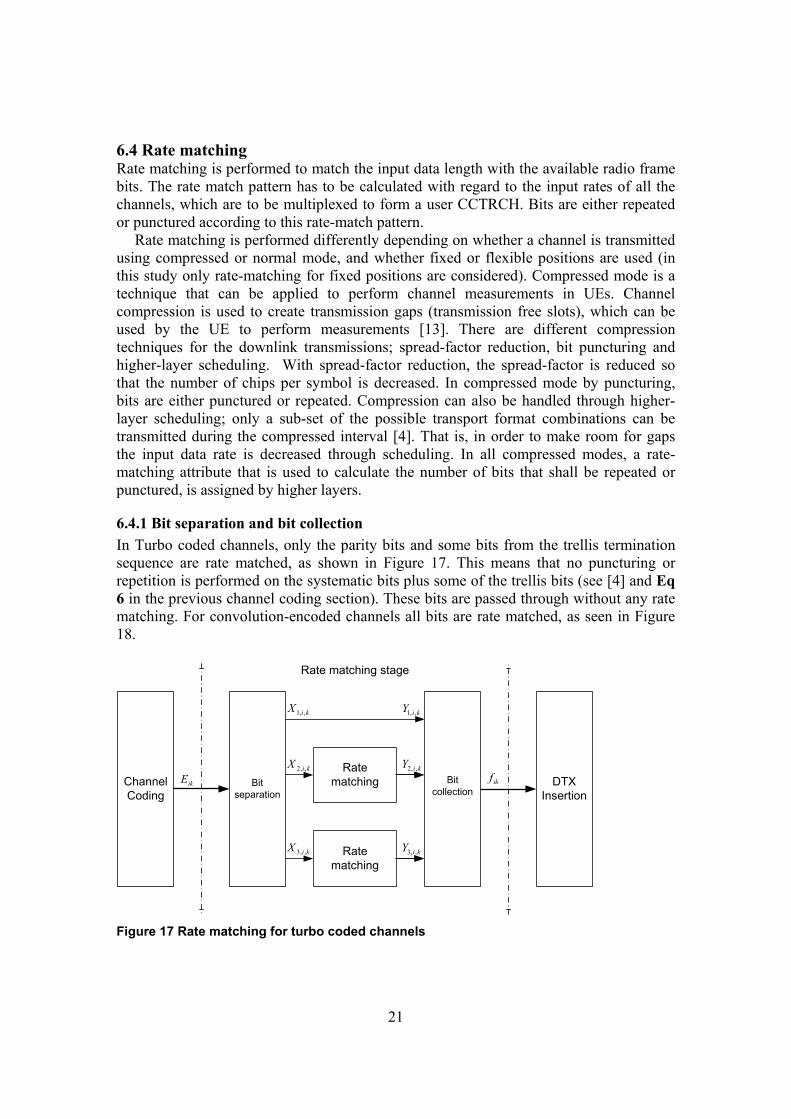
21
6.4 Rate matching Rate matching is performed to match the input data length with the available radio frame bits. The rate match pattern has to be calculated with regard to the input rates of all the channels, which are to be multiplexed to form a user CCTRCH. Bits are either repeated or punctured according to this rate-match pattern. Rate matching is performed differently depending on whether a channel is transmitted using compressed or normal mode, and whether fixed or flexible positions are used (in this study only rate-matching for fixed positions are considered). Compressed mode is a technique that can be applied to perform channel measurements in UEs. Channel compression is used to create transmission gaps (transmission free slots), which can be used by the UE to perform measurements [13]. There are different compression techniques for the downlink transmissions; spread-factor reduction, bit puncturing and higher-layer scheduling. With spread-factor reduction, the spread-factor is reduced so that the number of chips per symbol is decreased. In compressed mode by puncturing, bits are either punctured or repeated. Compression can also be handled through higher-layer scheduling; only a sub-set of the possible transport format combinations can be transmitted during the compressed interval [4]. That is, in order to make room for gaps the input data rate is decreased through scheduling. In all compressed modes, a rate-matching attribute that is used to calculate the number of bits that shall be repeated or punctured, is assigned by higher layers.
6.4.1 Bit separation and bit collection In Turbo coded channels, only the parity bits and some bits from the trellis termination sequence are rate matched, as shown in Figure 17. This means that no puncturing or repetition is performed on the systematic bits plus some of the trellis bits (see [4] and Eq 6 in the previous channel coding section). These bits are passed through without any rate matching. For convolution-encoded channels all bits are rate matched, as seen in Figure 18.
ChannelCoding
DTXInsertion
Ratematching
Bitseparation
Bitcollection
Ratematching
Rate matching stage
kiX ,,1
kiX ,,2
kiX ,,3
kiY ,,1
kiY ,,2
kiY ,,3
ikE ikf
Figure 17 Rate matching for turbo coded channels

22
The variable iE describes the number of input bits to the rate-matching function after channel coding. The relations between the number of input and output bits for turbo-coded channels are
3/,,3,2,11)1(3,,,1 iiikiki EXXkCX === +− K 3/,,3,2,12)1(3,,,2 iiikiki EXXkCX === +− K 3/,,3,2,13)1(3,,,3 iiikiki EXXkCX === +− K
For convolution coded channels and turbo coded channels using repetition the relation is
iiikiki EXXkCX === ,,3,2,1,,,1 K
ChannelCoding
DTXInsertion
Bitseparation
Bitcollection
RateMatchingAlgorithm
Rate matching stage
Ci,k Xi,k Yi,k Zi,k
Figure 18 Rate matching for convolution coded channels
The bits are collected into a single output sequence after the rate matching. The bit positions that are punctured during the rate matching are marked with a third value, δ, where δ∉{0,1}. The δ bits can be removed directly after bit collection. For turbo encoded channels with puncturing the output sequence is
ikik YkYZ ,,3,2,1,,11)1(3,1 K==+−
ikik YkYZ ,,3,2,1,,22)1(3,1 K==+−
ikik YkYZ ,,3,2,1,,33)1(3,1 K==+− For convolution encoded channels and turbo encoded channels using repetition the relation is
ikik YkYZ ,,3,2,1,,1,1 K==

23
6.4.2 Calculation of rate matching parameters for fixed positions The rate matching parameters are used to compute puncture and repetition patterns. The pattern is computed as described by an algorithm, presented in sub-section 4.2.7.5 in [4], where also the equations required for calculation of intermediate variables (Eq 3 to Eq 6 shown below) can be found. The number of available data bits within a CCTRCH is denoted jdataN , , where j is the transport format combination used. This variable is dependant on the number of physical channels and the spread factor used for the specific user CCTRCH. The number of physical channels is denoted by P. The total number of bits available for a user CCTRCH can be calculated as ( )21,* 15 datadatadata NNPN +××= , where 1dataN and 1dataN depend on the slot format used. These slot formats are specified in Table 11 in [14].
Eq 3 ( )
⎟⎠⎞⎜
⎝⎛×=
∈
TTIliiTFSl
ii N
FN ,,* max1
Eq 4
⎥⎥⎥⎥⎥
⎦
⎥
⎢⎢⎢⎢⎢
⎣
⎢
×
⎟⎟⎠
⎞⎜⎜⎝
⎛×⎟⎠
⎞⎜⎝
⎛×
=
∑
∑
=
=
i
mjmm
jdata
i
mjmm
ji
NRM
NNRMZ
1,
,1
,
, Ii L1=∀
Eq 5 jijijiji NZZN ,,1,, −−=Δ − Ii L1=∀
Eq 6 ,*max, iii NFN Δ×=Δ
6.4.3 Parameters for normal mode and compressed mode by spread factor reduction The number of bits to be punctured or repeated per TTI is denoted TTI
liN ,Δ , where i is the
transport channel and l the transport format. A negative value of TTIliN ,Δ corresponds to
the number of bits to be punctured and a positive number corresponds to the number of bits to be repeated. The output data rate is equal to the input data rate if 0max, =Δ iN for TRCH i. Thus, the rate-matching algorithm, as specified in [4], shall not be executed. This means that the number of bits for all transport channels to be repeated or punctured is 0, as described by Eq 6.
Eq 6 0, =Δ TTIliN )(iTFSl ∈∀ .
The rate-matching algorithm shall be executed if 0max, ≠Δ iN , after calculation of the vari-ables eini, eplus and eminus.
Parameters for compressed mode by puncturing The variables ,*iN and ,*iNΔ are calculated in the same way as in the compressed mode by spread factor reduction, i.e. using Eq 3 to Eq 5.
Eq 7 ,*max, iimi NFN Δ×=Δ

24
The number of bits to be removed on TRCH i (to create the gap for compressed mode and to compensate for reduction of bits in the slot format compared to normal slot format), is denoted n
iNp max, . The value of niNp max, is calculated for each radio frame n of the
TTI and ( )1max, −−= iini ZZNp for i=1 to I
Eq 8 [ ] ( )( )
⎥⎥⎥⎥⎥
⎦
⎥
⎢⎢⎢⎢⎢
⎣
⎢
×
⎟⎟⎠
⎞⎜⎜⎝
⎛−+×⎟
⎠
⎞⎜⎝
⎛×
=
∑
∑
=
=
i
mjmm
datadataTGL
i
mjmm
ji
NRM
NNNNNRMZ
1,
,*,*1
,
,
'
The variable NTGL is the number of bits in each radio frame corresponding to the gap. The number of empty slots is denoted TGL and the first empty slot in the gap is denoted Nfirst.
( )⎪⎪⎪
⎩
⎪⎪⎪
⎨
⎧
>+×−−
>+×−
≤+×
=
15'1515
15'15
15
15'15
,*
,*
,*
TGLNifframeradiofollowinginNNTGL
TGLNifgaptheofframeradiofirstinNN
TGLNifNTGL
N
firstdatafirst
firstdatafirst
firstdata
TGL
The total number of bits in the gaps when applying compressed mode is calculated as ( )
∑−×+=
×=
=11
max,,
max,
i
i
Fmn
Fmn
ni
mTTIi NpNp
AMR service Input and output data flows for rate matching of the AMR service, using the highest AMR data rate, are illustrated in Figure 19. The rate matching function is one of the more problematic functions in the baseband because the data streams must be manipulated on single bit level (puncturing and repetition of bits) according to the channel specific rate matching pattern. There is no obvious way to vectorize the matching computation since the bit stream lengths and rate match patterns are different for each transport channel. More obvious is that each transport channel stream can be calculated in MIMD fashion.
After rate matching
333 132
326 338 176
Input afterconvolution coding
DCH A DCH B DCH C
303
Figure 19 AMR output after rate matching
The following fixed parameters can be used for implementation of the rate matching function for AMR

25
• Static rate matching parameter for 180 DCH A, 170 for DCH B and 215 for DCH C • Compression parameters used for punctured normal/punctured channels
o Normal mode, bits per CCTRCH is ( )226151,* +××=dataN o Compressed mode, bits per CCTRCH is ( )4012151,* +××=dataN
• Compression parameters for normal/spread factor reduction channels o Normal mode, bits per CCTRCH is ( )226151,* +××=dataN o Compressed mode, bits per CCTRCH is ( )4412151,* +××=dataN
High bit-rate data service Like with the AMR data streams, there is no obvious way to vectorize computation of the data streams but the rate matching function be mapped in a MIMD parallel fashion. A bit-rate of 2048 kbps requires a channel spread factor of length 4. Compressed mode by spread factor reduction is not supported for spread factors of length 4, which means that only normal mode, higher layer scheduling and compressed mode by puncturing can be applied. The input constitutes 0 to 16 parallel channel streams, each with sM code blocks of length maxN , where ,*max datas NNM ≤× . ( ,*dataN can maximally be 248 + 992 when using SF of length 4).
DCH 1
0 - n1
DCH 1
After rate matchingrm bits added
mi blocks of size 0 - niwhere i is 0 - 16
channelsDCH 2
0 - n2
DCH 2
DCH i
0 - ni
DCH i
0 0 0 ni + rmn2 + rmn1 + rm Figure 20 Rate matching on data streams
6.5 First insertion of discontinuous transmission (DTX) indication bits Unused bits in the radio frames are filled with DTX bits. The DTX bits are never transmitted over the air, they are used just to mark when transmission should be turned off. This first DTX insertion is performed only if fixed channel positions in the radio frames are used, see Figure 21. With fixed positions it means that a fixed number of bits are reserved for each transport channel in the radio frames. If bits were punctured in the rate-matching, the space required for the punctured bits should be reserved for later insertion of p bits.

26
TFCI TRCH A TPC TRCH B PILOTDTX
TFCI TRCH A TPC TRCH B PILOT
Downlink transmission using 2 DCHs
Full rate
DCH A Half rate
Figure 21 Fixed channel slots with variable rate and insertion of DTX bits
For radio frames in which flexible positions are used, the DTX insertion is performed
after the multiplexing of the transport channels. The decision of using fixed or flexible positions is controlled from higher layers in the UTRAN. The bit output after the DTX insertion is three-valued {0, 1, δ}.
The bits after rate matching are denotediiGiii gggg ,,,, 321 K , where Gi is the number
of bits in one TTI of Trch i. The number of bits available for a radio frame in Trch i is denoted Hi and the number of radio frames per TTI for Trch i is Fi. The total number of bits after DTX insertion is denoted Di. If no compression or compressed mode by spread factor reduction is performed, then iii HFD ×= . If compressed mode by puncturing is used, space for the bits that were punctured in the rate matching function should be reserved. This space will be used for insertion of p bits in the proceeding interleave function. For compressed mode by puncturing, DTX bits should be inserted until
mTTIiiii NpHFD ,
max,−×= and ,*,* iii NNH Δ+= . The variables ,,*iN ,*iNΔ and mTTIiNp ,
max, were defined for the rate matching function. The bits after DTX insertion are denoted
iiDiii hhhh ,,,, 321 K . The input and output relation after DTX insertion is:
ikik gh = for iGk ,,3,2,1 K= δ=ikh for iiii DGGGk ,,3,2,1 K+++=
AMR service In this specific case for the AMR service it is assumed that processing is performed in normal mode. Bit repetition is performed in the previous rate matching function to fill up the radio frames. Therefore no DTX insertion is required in this case. The output after DTX insertion are represented by two bits, thus, the output data size is doubled. Each bit after DTX insertion is three-valued and therefore each symbol is represented by two bits.
After DTX insertion
338 176
2*326 2*338 2*176
Input after rate matchingDCH A DCH B DCH C
326
Figure 22 Output after DTX insertion. Each symbol is three-valued {0, 1, δ} and represented using two bits
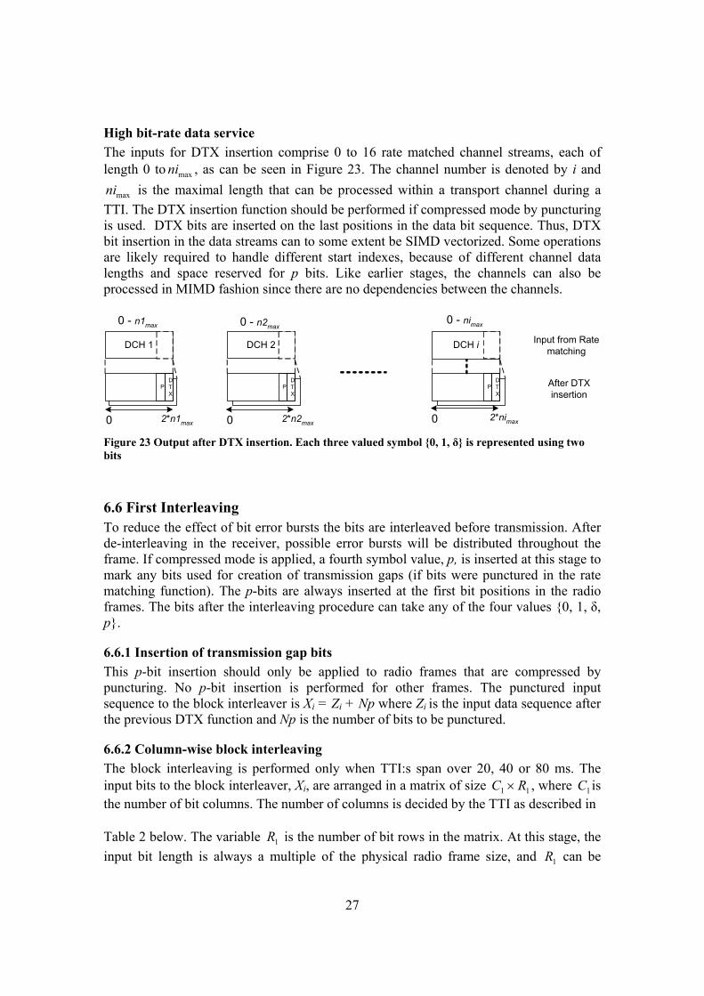
27
High bit-rate data service The inputs for DTX insertion comprise 0 to 16 rate matched channel streams, each of length 0 to maxni , as can be seen in Figure 23. The channel number is denoted by i and
maxni is the maximal length that can be processed within a transport channel during a TTI. The DTX insertion function should be performed if compressed mode by puncturing is used. DTX bits are inserted on the last positions in the data bit sequence. Thus, DTX bit insertion in the data streams can to some extent be SIMD vectorized. Some operations are likely required to handle different start indexes, because of different channel data lengths and space reserved for p bits. Like earlier stages, the channels can also be processed in MIMD fashion since there are no dependencies between the channels.
0 - n1max
DCH 1
P After DTXinsertion
0 - n2max0 - nimax
0 2*n1max 0 2*n2max 0 2*nimax
DTX
DCH 2
PDTX
DCH i
PDTX
Input from Ratematching
Figure 23 Output after DTX insertion. Each three valued symbol {0, 1, δ} is represented using two bits
6.6 First Interleaving To reduce the effect of bit error bursts the bits are interleaved before transmission. After de-interleaving in the receiver, possible error bursts will be distributed throughout the frame. If compressed mode is applied, a fourth symbol value, p, is inserted at this stage to mark any bits used for creation of transmission gaps (if bits were punctured in the rate matching function). The p-bits are always inserted at the first bit positions in the radio frames. The bits after the interleaving procedure can take any of the four values {0, 1, δ, p}.
6.6.1 Insertion of transmission gap bits This p-bit insertion should only be applied to radio frames that are compressed by puncturing. No p-bit insertion is performed for other frames. The punctured input sequence to the block interleaver is Xi = Zi + Np where Zi is the input data sequence after the previous DTX function and Np is the number of bits to be punctured.
6.6.2 Column-wise block interleaving The block interleaving is performed only when TTI:s span over 20, 40 or 80 ms. The input bits to the block interleaver, Xi, are arranged in a matrix of size 11 RC × , where 1C is the number of bit columns. The number of columns is decided by the TTI as described in Table 2 below. The variable 1R is the number of bit rows in the matrix. At this stage, the input bit length is always a multiple of the physical radio frame size, and 1R can be

28
calculated asi
i
CX
R =1 . The input bits are arranged row wise in sequential order as shown
in Figure 24.
( ) ( ) ( ) ( )
( )( ) ( )( ) ( )( ) ( )( ) ( ) ⎥⎥⎥⎥⎥
⎦
⎤
⎢⎢⎢⎢⎢
⎣
⎡
×+×−+×−+×−+×−
×+++
11,4111,3111,2111,1111,
12,21,21,11,
1,3,2,1,
...............
...
CRiCRiCRiCRiCRi
CiCiCiCi
Ciiii
XXXXX
XXXXXXXX
Figure 24 Bit input arrangement before interleaving
The bit matrix shall be interleaved column-wise. The permutation pattern that shall be used for interleaving is described in Table 2. The number sequence in the table corresponds to the original positions in the input matrix from where the bits should be read. As can be seen in the table, no interleaving is performed during TTIs of 10 ms. When the columns have been interleaved the output bits should be read column-wise in sequential order, starting with the leftmost column. Table 2 Number of columns and permutation pattern for interleaving
TTI Number of columns (C1) Column-wise permutation pattern ( ) ( ) ( )111,...,11,01 111 −CPPP CCC
10 ms 1 0 20 ms 2 1,0 40 ms 4 3,1,2,0 80 ms 8 7,3,5,1,6,2,4,0
AMR service The interleaving function is performed for all three channel streams that are used to map the AMR data. The TTI is 20 ms and therefore, according to Table 2, the data must be arranged in a two-column bit matrix. The output after interleaving will be four-valued symbols ∈ {0, 1, δ, p}, which require two bits to represent each symbol, as illustrated in Figure 25. The column interleaving pattern is the same for three used transport channels and it is possible to SIMD vectorize parts of the interleaving function. Alternatively, the streams can be processed in MIMD fashion like the earlier functions.
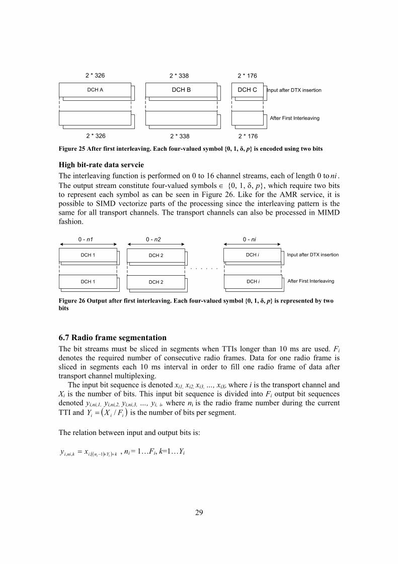
29
After First Interleaving
2 * 338 2 * 176
Input after DTX insertionDCH A DCH B DCH C
2 * 326
2 * 338 2 * 1762 * 326 Figure 25 After first interleaving. Each four-valued symbol {0, 1, δ, p} is encoded using two bits
High bit-rate data servcie The interleaving function is performed on 0 to 16 channel streams, each of length 0 to ni . The output stream constitute four-valued symbols ∈ {0, 1, δ, p}, which require two bits to represent each symbol as can be seen in Figure 26. Like for the AMR service, it is possible to SIMD vectorize parts of the processing since the interleaving pattern is the same for all transport channels. The transport channels can also be processed in MIMD fashion.
DCH 1 After First Interleaving
Input after DTX insertionDCH 1
DCH 2
DCH 2
DCH i
DCH i
0 - n1 0 - n2 0 - ni
Figure 26 Output after first interleaving. Each four-valued symbol {0, 1, δ, p} is represented by two bits
6.7 Radio frame segmentation The bit streams must be sliced in segments when TTIs longer than 10 ms are used. Fi denotes the required number of consecutive radio frames. Data for one radio frame is sliced in segments each 10 ms interval in order to fill one radio frame of data after transport channel multiplexing.
The input bit sequence is denoted xi1, xi2, xi3, …, xiX, where i is the transport channel and Xi is the number of bits. This input bit sequence is divided into Fi output bit sequences denoted yi,ni,1, yi,ni,2, yi,ni,3, …, yi, i, where ni is the radio frame number during the current TTI and ( )iii FXY /= is the number of bits per segment. The relation between input and output bits is:
( )( ) kYniknii iixy +×−= 1,,, , ni = 1…Fi, k=1…Yi

30
AMR service The AMR input for the frame segmentation comprise 3 channel streams and the TTI is 20 ms. Thus, the streams will be sliced in two segments which are distributed over two radio frames, as shown in Figure 27. The first segment comprises the bits 1 to 163 in DCH A, bits 1 to 169 in DCH B and bits 1 to 88 in DCH C. The second segment comprises the bits 164 to 326 in DCH A, is bits 170 to 338 in DCH B and is bits 89 to 176 in DCH C. The transport channels with a composite user channel (DCH A, DCH B and DCH C) comprise bit streams of different lengths. However, segmentation can be more efficiently SIMD vectorized by grouping channels from several user channels in groups of class A bits channels, class B bits channels and class C bits channels, i.e. DCH A channels from several users are combined and SIMD vectorized. Alternatively, the channels can be processed in MIMD fashion since there are no data dependencies between transport channels in the frame segmentation function.
After framesegmentation
Input after firstinterleaving
DCH A DCH B DCH C
Fra-me 1
Fra-me 2Frame 1 Frame 2 Frame 1 Frame 2
326 338 176
1 163 164 326 1 169 170 338 1 88 89 176 Figure 27 After frame segmentation {0, 1, δ, p}
High bit-rate data service The input which is mapped on 0 to 16 channel streams for the high bit-rate data service will be sliced in segments dependently on the TTI and the number of physical radio frames used. At maximum, three physical channels can be used for a single user. Each
channel data stream will be sliced in m frame segments, where m is 10
TTI (10 ms multiple
of the TTI). The frames are sliced in blocks of equal lengths, which makes it possible to SIMD vectorize the slicing operation. Like earlier functions, it is also possible to perform the slicing operation in MIMD fashion since there are no data dependencies between the channels.
After framesegmentation
Input after firstinterleaving
where i is 0 to 16channels
DCH 1
Frame1
Frame2
n1
Framem
DCH i
Frame1
Frame2
nI
Framem
DCH 2
Frame1
Frame2
n2
Framem
Figure 28 After frame segmentation {0, 1, δ, p}

31
6.8 Transport channel (Trch) multiplexing Radio frame segments are delivered to the multiplexer function with a 10 ms interval, corresponding to the radio frame transmission frame rate. These frame segments from different transport channels are multiplexed to form a single user CCTRCH stream (only one CCTRCH is possible for one UE). The CCTRCH will later be mapped on one or several physical channels. The transport channels that are to be multiplexed to the same CCTRCH must use the same spreading factor. The input bits are denoted fi1, fi2, fi3,… fiVi where Vi is the number of bits for transport channel i. The number of transport channels is I. The bit output after channel multiplexing is s1, s2, s3,… sS where S is the number of bits corresponding to the number of physical radio frames used, ∑=
iiVS
AMR service The multiplexing function constitutes a synchronization stage in the function pipeline. The input constitutes one segment from each of the three used transport channels for the AMR service. These are multiplexed into a single output stream, as shown in Figure 29. The TTI for AMR is 20 ms which means that multiplexing is performed twice during a TTI to fill two consecutive radio frames. If the previous functions were processed in MIMD fashion, the multiplex function will comprise a merge of multiple channel input streams. If the previsous functions were processed by SIMD vectorizarion, the multiplex function will comprise rearrangement and merging of vectorized data, dependently on how the streams were SIMD vectorized.
One singleCCTRCH streamafter multiplexing
After Framesegmentation
420420
DCHC
DCHCDCH A DCH ADCH B DCH B
DCH A DCH B DCHCDCH A DCH B DCH
C
10 ms 10 ms
First radioframe
Second radioframe
Figure 29 Before and after transport channel multiplexing in AMR processing
High bit-rate data service The input constitutes I segments, one from each of I channel streams, and which are multiplexed into a single output stream, as shown in Figure 30. Like with the AMR processing, the multiplexing constitutes a synchronization stage in the function flow. If the previous functions were processed by SIMD vectorizarion, the multiplex function will comprise rearrangement and merging of vectorized data, dependently on how the streams were SIMD vectorized. If the previous functions were processed in MIMD fashion, the multiplex function will comprise a merge of multiple channel input streams.
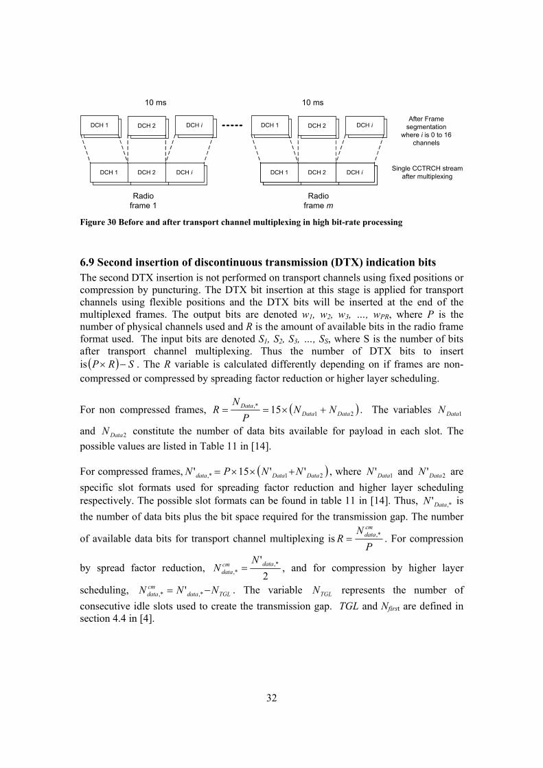
32
DCH 1 DCH 2 DCH iDCH 1 DCH 2 DCH i
Single CCTRCH streamafter multiplexing
After Framesegmentation
where i is 0 to 16channels
Radioframe 1
Radioframe m
10 ms 10 ms
DCH 1 DCH 2 DCH i DCH 1 DCH 2 DCH i
Figure 30 Before and after transport channel multiplexing in high bit-rate processing
6.9 Second insertion of discontinuous transmission (DTX) indication bits The second DTX insertion is not performed on transport channels using fixed positions or compression by puncturing. The DTX bit insertion at this stage is applied for transport channels using flexible positions and the DTX bits will be inserted at the end of the multiplexed frames. The output bits are denoted w1, w2, w3, …, wPR, where P is the number of physical channels used and R is the amount of available bits in the radio frame format used. The input bits are denoted S1, S2, S3, …, SS, where S is the number of bits after transport channel multiplexing. Thus the number of DTX bits to insert is ( ) SRP −× . The R variable is calculated differently depending on if frames are non-compressed or compressed by spreading factor reduction or higher layer scheduling.
For non compressed frames, ( )21,* 15 DataData
Data NNP
NR +×== . The variables 1DataN
and 2DataN constitute the number of data bits available for payload in each slot. The possible values are listed in Table 11 in [14]. For compressed frames, ( )21,* ''15' DataDatadata NNPN +××= , where 1'DataN and 2'DataN are specific slot formats used for spreading factor reduction and higher layer scheduling respectively. The possible slot formats can be found in table 11 in [14]. Thus, ,*'DataN is the number of data bits plus the bit space required for the transmission gap. The number
of available data bits for transport channel multiplexing isP
NR
cmdata,*= . For compression
by spread factor reduction, 2
' ,*,*
datacmdata
NN = , and for compression by higher layer
scheduling, TGLdatacmdata NNN −= ,*,* ' . The variable TGLN represents the number of
consecutive idle slots used to create the transmission gap. TGL and Nfirst are defined in section 4.4 in [4].

33
( )⎪⎪⎪
⎩
⎪⎪⎪
⎨
⎧
>+×−−
>+×−
≤+×
=
15sec,'1515
15,'15
15
15,'15
,*
,*
,*
TGLNifframeondinNNTGL
TGLNifframefirstinNN
TGLNifNTGL
N
firstdatafirst
firstdatafirst
firstdata
TGL
The relation between the input bits and output bits is:
Sksw kk ...,,3,2,1== RPSSSkwk ×+++== ...,,3,2,1δ
DTX indication bits are denoted by δ { }p,1,0∉ and non DTX bits Sk { }p,1,0∈ .
AMR service The AMR input constitutes a single stream of data segmented into two radio frames, see Figure 31. In the AMR service it was assumed that fixed frame positions are used and therefore no DTX insertion is required at this stage.
After 2'nd DTX insertion
CCTRCH Multplexing
420420
First radio frame Second radio frame
Frame 1 Frame 2
Frame 1 Frame 2
Figure 31 After second DTX insertion
High bit-rate data service The input constitutes a single stream of data segmented into n frames, where n is a 10 ms multiple of the TTI, see Figure 32. Fixed frame positions are assumed to be used, so no DTX insertion is required at this stage.
After 2'nd DTX insertion
CCTRCH Multplexing
First radioframe
Frame 1
Frame 1
Second radioframe
Frame 2
Frame 2
Third radioframe
Frame 3
Frame 3
n'th radio frame
Frame n
Frame n
Figure 32 Output after second DTX insertion.

34
6.10 Physical channel segmentation When several physical channels are used, the input must be segmented in blocks, as many as the number of physical channels used for the user CCTRCH. If compressed mode by puncturing is used, the p-bits inserted earlier, during the interleaving procedure, are removed before they are mapped on physical channels. For all other modes, all bits are mapped onto the physical channels. 1-8 simultaneous DPCH codes can be received simultaneously [4]. The input bits are denoted x1, x2, x3, …, xM, where M is the total number of bits before physical channel segmentation. The bits after channel segmentation are denoted U and the number of physical channels P. For all modes, except compressed
mode by puncturing, the relation is PXU = . For compressed mode by puncturing, the
relation is ( )( ) PNNNXU datadataTGL /' ,*,* −−−= . The variables are explained above in subsection 6.9.
AMR service Only one physical channel is required for the AMR service and therefore no physical channel segmentation is required. Thus, the channel stream is unmodified at this stage, as shown in Figure 33.
After Physical ChannelSegmentation
After 2'nd DTX insertion
420420
First radio frame in CCTRCH Second radio frame inCCTRCH
Frame 1 Frame 2
Frame 1 Frame 2
Figure 33 After physical channel segmentation
High bit-rate data service The maximum number of physical channels that can be used for the studied UE class is limited to three. See Figure 34 for an illustration of the physical channel segmentation.
After Physical ChannelSegmentation
First radio frame in CCTRCH Second radio frame in CCTRCH
Phy 1 Phy 2 Phy 3
Frame 2
Frame 1
Frame n
Third radio frame in CCTRCH Figure 34 Frames are segmented on separate on maximum 3 physical channels

35
The segments can either be distributed in MIMD fashion, into separate data streams for each channel, or kept in a single stream in order to process the data using SIMD vectorization in the following functions.
6.11 Second Interleaving Before radio frames are mapped onto physical channels, a second interleaving procedure is performed. This interleaving is performed for each physical channel, if multiple physical channels are used. The bits in the radio frames are arranged in a bit matrix. The number of columns in the matrix, denoted C2, is always constant. Thus, the number of rows in the matrix is determined by the input length. If the number of input bits is not equal to the minimum possible matrix size, bits with zeros or ones are padded to the bit positions which correspond to the end of the frame. These pad bits will be removed after the interleaving. The interleaving is then performed by swapping whole columns in the matrix according to a constant interleaving pattern. After the interleaving, the bits are read in a transposed matrix order (i.e. column-wise instead of row-wise).
Interleaving Algorithm I. The number of columns are numbered 0, 1, 2, …, C2-1, where C2 always is 30
and the order is from left to right. II. The number of rows in the bit matrix, denoted R2, is determined by finding the
minimum R2 such that 22 RCU ×≤ , where U is the number of input bits on the physical channel p. The rows are numbered 0, 1, 2, …, R2-1, from the top to the bottom.
III. The input bit sequence up,1, up,2, up,3, …, up,U is written in sequential order, row-
wise into the bit matrix starting at column 0, row 0:
( ) ( ) ( ) ( )
( )( ) ( )( ) ( )( ) ( ) ⎥⎥⎥⎥⎥
⎦
⎤
⎢⎢⎢⎢⎢
⎣
⎡
×+×−+×−+×−
×+++
22,3212,2212,1212,
22,32,22,12,
2,3,2,1,
CRpCRpCRpCRp
CpCpCpCp
Cpppp
yyyy
yyyyyyyy
L
MLMMM
L
L
IV. The bit matrix shall be permuted according to the pattern ( )
}12,...,1,0{2
−∈ CjjP where
j is the original column position. The permutation pattern is shown in Table 3, where )(2 jP is the value at the original position j, and the column position after interleaving is determined by the corresponding index in the sequence in Table 3 (on row 2).

36
Table 3 Inter-column permutation pattern for second interleaving
Number of columns (C2) Permutation pattern )12(2),...,1(2),0(2 −CPPP
30
⟩⟨
17,27,22,7,2,12,29,9,19,24,14,4,26,16,6,21,11,1,28,18,8,23,13,3,25,15,5,10,20,0
V. The output after block interleaving should be read column-wise from the bit
matrix. After the interleaving, bits in the 22 RC × bit matrix are denoted kpy ,' .
( ) ( ) ( ) ( )
( )( ) ( )( ) ( )( ) ( ) ⎥⎥⎥⎥⎥
⎦
⎤
⎢⎢⎢⎢⎢
⎣
⎡
×+×−+×−+×−
×+++
22,3212,2212,1212,
22,32,22,12,
2,3,2,1,
CRpCRpCRpCRp
CpCpCpCp
Cpppp
yyyy
yyyyyyyy
L
MLMMM
L
L
The pad bits that were added in order to compensate the size if 22 RCU ×< should be deleted before the interleaved bits are mapped on the physical channels.
AMR service The input constitutes one single channel stream of new radio frame data each 10 ms, two radio frames per TTI as shown in Figure 35. It is possible to perform parts of the interleaving procedure in SIMD vectorized fashion, depending on how the input data is arranged and how the output data must be arranged for the following function.
After 2'nd Interleaving
After Physicial ChannelSegmentation
Phy Frame 1
Phy Frame 1
Phy Frame 2
Phy Frame 2
Figure 35 After second interleaving
High bit-rate data service The input comprises one single channel stream of maximum three radio frames, or three separate streams (one frame mapped on each stream), delivered for each 10 ms interval dependent on how data was arranged after the segmentation function, see Figure 36.
After 2'nd Interleaving
After Physicial ChannelSegmentation
Phy Frame 1
Phy Frame 1
Phy Frame 2
Phy Frame 2
Phy Frame 3
Phy Frame 3
Figure 36 After second interleaving

37
Like with the AMR service, parts of the interleaving function can be performed in SIMD parallel fashion depending on the arrangement on the input data and how the data is required to be arranged for the following function.
6.12 Physical channel mapping After the second interleaving, the bits are ready to be mapped on the physical
channels [14]. The input bits for physical channel mapping are denoted Uppp vvv ,2,1, ,...,, , where p is the number of physical channels used and U is the number of bits to be transmitted in one radio frame (for each physical channel). The bits are mapped so that they are transmitted in ascending order via the air interface. Not all bits are necessarily sent over the air. Bits that have values { }1,0, ∉kpv correspond to DTX indicators or p-bits. The DTX indicators are mapped on the frames but the transmission is turned off. When compressed mode is applied, certain slots will be empty, i.e. no bits are mapped to those slots (the p-bits inserted in the interleaving function). If 15<+TGLN first , all empty slots are mapped within a single frame. When 15>+TGLN first , the empty slots are mapped over two consecutive frames. If the TGL span over two frames, the empty slots in the first frame should be 14,,, ,...21 ++ firstfirstfirst NNN . In the second frame the empty slots shall be lastN,...,2,1,0 . When compressed mode by spread factor reduction is used, bits are mapped only using 7.5 slots.
AMR service One composite input stream; one radio frame per 10 ms is mapped on 15 physical slots, see Figure 37.
After Physical Mapping
After 2'nd Interleaving
15 radio frame slots
First radio frame inCCTRCH
Second radio frame inCCTRCH
Frame 1 Frame 2
15 radio frame slots Figure 37 After AMR physical channel mapping
High bit-rate data service The input comprise of up to 3 channel streams depending on the bit-rate requirements; one frame for each 10 ms interval is mapped using 15 slots, for each physical channel, see Figur 38.

38
After 2'nd Interleaving
15 radio frame slotsPhy channel 1
Phy Frame 1 Phy Frame n
15 radio frame slotsPhy channel n
Figur 38 After data physical channel mapping
7. Summary This report concluded a study performed of required baseband processing in 3G UMTS radio base stations. The study is focused on the processing required for certain transmission modes in the RBS downlink using downlink dedicated transport channels (DCH:s). Two examples of user services – an AMR voice call service and a generalised case of high bit-rate data transmissions – have been used to abstractly describe and discuss processing characteristics and different ways of mapping the dataflows and dependencies through the baseband function flow. The service examples can be used as test cases for evaluation and mapping of software implemented baseband functions. The functions are logically arranged in a pipelined sequence, operating on periodic input and output bit streams of user data. The 3G network standard is designed to support simultaneous service transmission by allocation of multiple parallel transport channels for a single mobile user. It was illustrated through abstract mapping of the two presented service examples that the function interdependencies are of producer/consumer type. Moreover, it was discussed how different kinds of parallelism can be exploited in the functions, with respect to the data stream-lengths, the number of transport blocks and allocated channels, as well as requirements for control operations to map bit stream data processing on word-length architectures. Thus it was concluded that several functions has the potential to be mapped in parallel; both in the time and the spatial domain, through exploitation of SIMD or MIMD parallelism.
Transport channels are multiplexed in the function pipeline to form a single composite transport channel. Depending on bandwidth requirements, it was illustrated that the composite channels are segmented and mapped on multiple physical channels. These multiplex, de-multiplex functions require synchronisation of data streams at several processing stages.
The operations performed by the baseband functions (in the down link), are of logical rather than arithmetical nature. Seen from an abstract functional level, the required data operations are dominated by shuffling, padding and logical manipulation on bit-field data. To be able to efficiently implement and compile the baseband functions to an architecture abstraction, based on parallel and reconfigurable processor architectures, it must be possible express the application characteristic properties in the supported programming model. Desirably, it should be possible to express bit field data types and operations as well as data and instruction parallelism on several granularity levels; function- and instruction-level parallelism.

39
Appendix A: Glossary 3GPP 3G Partnership Project AMR Adaptive Multi Rate ASIC Application Specific Integrated Circuit CCH Control Channel CCTRCH Coded Composite Transport CHannel CDMA Code Division Multiple Access CN Core Network DCH Dedicated Channel DSP Digital Signal Processor DTX Discontinuous Transmission bits EDGE Enhanced Data rate for GSM Evolution FACH Forward Access Channel FDD Frequency Division Duplex FEC Forward Error Correction FPGA Field Programmable Gate Array MAC Medium Access Control MIMD Multiple Instruction Multiple Data PCH Physical Channel RAB Radio Access Bearer RACH Random Access Channel RNC Radio Network Controller RNS Radio Network Sub system RRC Radio Resource Control SF Spreading Factor SIMD Single Instruction Multiple Data TDD Time Division Duplex TFCI Transport Format Combination Indicator TFI Transport Format Indicator TFS Transport Format Set TGL Transmission Gap Length TTI Transmission Time Interval UE User Equipment UMTS Universal Mobile Telecommunication Standard UTRAN UMTS Terrestrial Radio Access Network WCDMA Wideband Code Division Multiple Access
40
References [1] www.3gpp.org [2] H. Holma and A. Toskala, WCDMA for UMTS, 3rd edition, 2004, Wiley & sons [3] 3GPP, ”UTRAN Iur/Iub interface user plane protocol for DCH data streams”, TS
25.427, www.3gpp.org, Release 5 [4] 3GPP, ”Multiplexing and channel coding (FDD)”, TS 25.212, www.3gpp.org, Release
5 [5] 3GPP, ”Services provided by the physical layer”, TS 25.302, www.3gpp.org, Release
5 [6] 3GPP, ”Adaptive Multi-Rate (AMR) speech codec frame structure”, TS 26.101,
www.3gpp.org, Release 5 [7] 3GPP, ”Adaptive Multi-Rate (AMR) speech codec; Interface Iu, Uu and Nb”, TS
26.102, www.3gpp.org,, Release 5 [8] 3GPP, ”AMR Wideband Speech Codec; Frame structure ”, TS 26.201,
www.3gpp.org, Release 5 [9] 3GPP, ”UE Radio Access capabilities”, TS 25.306, www.3gpp.org, Release 5 [10] T. V. Ramabadran and S. S. Gaitonde, ”A Tutorial on {CRC} Computations”, IEEE-
MICRO, vol 8, no.4, aug, 1998, pp. 62-75 [11] Knuth, D., Art of Computer Programming, Volume 2: Semi numerical Algorithms,
3rd Edition , Addison Wesley, November 4, 1997 [12] E. Guizzo, “Closing in on the perfect code”, IEEE Spectrum, March 2004, pp. 28-34 [13] M. Gustafsson, K. Jamal, E. Dahlman, ”Compressed Mode Techniques for Inter-
frequency Measurements in a Wide-band DS-CDMA System”, The 8th IEEE Int. Symp. on Personal, Indoor and Mobile Radio Communications, 1997, vol.1, pp. 231-235
[14] 3GPP, ”Physical channels and mapping of transport channels onto physical channels (FDD)”, TS 25.211, www.3gpp.org, Release 5
Paper CA Configurable Framework for Stream Programming
Exploration in Baseband Applications
Bengtsson, J. and Svensson, B. (2006). A Configurable Framework for
Stream Programming Exploration in Baseband Applications. In Proc. of11th Int’l Workshop on High-Level Parallel Programming Models and Sup-portive Environments in conjunction with Int’l Parallel and Distributed Pro-cessing Symp. (IPDPS 2006), Rhodes, Greece.


A Configurable Framework for Stream ProgrammingExploration in Baseband Applications
Jerker Bengtsson and Bertil Svensson
Centre for Research on Embedded SystemsHalmstad University
PO Box 823, SE-301 18 Halmstad, Sweden{Jerker.Bengtsson, Bertil.Svensson}@ide.hh.se
Abstract
This paper presents a configurable framework to beused for rapid prototyping of stream based languages.The framework is based on a set of design patternsdefining the elementary structure of a domain spe-cific language for high-performance signal processing.A stream language prototype for baseband processinghas been implemented using the framework. We in-troduce language constructs to efficiently handle dy-namic reconfiguration of distributed processing param-eters. It is also demonstrated how new language spe-cific primitive data types and operators can be used toefficiently and machine independently express compu-tations on bit-fields and data-parallel vectors. Thesetypes and operators yield code that is readable, compactand amenable to a stricter type checking than is com-mon practice. They make it possible for a program-mer to explicitly express parallelism to be exploited bya compiler. In short, they provide a programming stylethat is less error prone and has the potential to leadto more efficient implementations.
1. Introduction
Advanced embedded high-performance applica-tions put very high requirements on computer sys-tems design. Some examples are modern radar sys-tems and baseband processing in radio base stations(RBS). Although the specific requirements are some-what different, the computational characteristics arequite similar. Traditionally this kind of applicationshave required development of ASICs and special pur-pose hardware to cope with the requirements. Par-allel architectures for high-performance applicationshas been a topic of research during many years. In re-cent years, results of this research and the advances insilicon process technology have opened up for a com-
modity market of highly parallel and reconfigurablearchitectures spanning from tens to several hundredsof processors on a single die [1, 2, 3].
Compiler technology and language development, onthe other hand, have not kept pace with the advancesin processor architecture. New approaches are re-quired in order to exploit the vast amount of exposedparallelism and communication structures. On theone hand, languages must offer constructs and opera-tions that allow a programmer to express parallelismand computations that are characteristic for a certainapplication domain. On the other hand, to enable ef-ficient compilation, languages must be structured fora machine abstraction that correlates well with thetarget architectures. These arguments speak in favorof a domain specific approach rather than a generalpurpose programming approach.
The goal of our research is to investigate anddevelop a stringent programming and compilationframework for domain specific high-performance ap-plications, targeting parallel and reconfigurable pro-cessors. In order to investigate what primitive lan-guage constructs, data types and operators are neededin an efficient programming language, our approach isto perform implementation experiments using realis-tic applications and experimental tools which can beused to quickly implement executable language proto-types. The application used for implementation stud-ies in this work is baseband processing performed in3G WCDMA radio base stations. An experimentalframework has been implemented in Java to be ableto perform quick prototype development and emula-tion of domain specific programming languages.
This paper is organized as follows. A backgroundand motivation for the work is given in Section 2.The configurable framework that has been developedfor implementation experiments is presented in Sec-tion 3. In Section 4, the language StreamBits whichhas been implemented for baseband processing is pre-

sented. Section 5 shows experiments that were con-ducted to demonstrate the applicability of the lan-guage. Finally, the paper is summarized with conclu-sions and future work in Section 6.
2. Background
The baseband provides the modem functionality ina wireless communication system and constitutes thecore in the 3G WCDMA technology. A radio basestation provides a set of full duplex physical data andcontrol channels, which are used to map higher layerdata packets to physical radio frames. [4]. The base-band resources of an RBS are managed by a higherlayer Radio Network Controller (RNC), which is re-sponsible for traffic scheduling on the physical userchannels provided by the baseband. The computa-tions performed in the RBS mainly constitute dataflows of bit-intensive protocol and signal processing,where the processing is controlled by service parame-ters given by the RNC. A baseband processing boardis a complex unit, for which many design parametershave to be considered. Besides meeting the hard re-quirements in performance, it must provide scalabilityand be sustainable for evolutions in standards. At thesame time, customers want low-cost RBS product so-lutions [5]. The life cycle of an RBS is measured inseveral decades, not years. To decrease initial productdevelopment costs it is an advantage if COTS compo-nents can be used to as large an extent as possible.Even if in-house ASIC solutions are hard to competewith in terms of performance and energy efficiency,they require large volumes in order to be a cost effi-cient solution. Also, considering the life cycle of anRBS, it is desirable not to encapsulate more function-ality than necessary into ASICs at early product gen-erations. New standard network functionalities areconstantly released and it must be possible to incorpo-rate these in existing platforms with minimal changesin hardware.
To meet these kinds of requirements in system de-sign, the trend is that more of the baseband function-alities are implemented using programmable solutions.One approach to support hardware flexibility is to ab-stract the baseband implementation through defini-tion of an application programming interface (API).Thus, the physical implementation of the basebandprocessing components can be disregarded by the pro-grammer, and the functionality of the components canbe implemented in either software or hardware.
2.1 Parallel and reconfigurable proces-sors
Of specific interest for the addressed applicationdomain are the array structured parallel and recon-
figurable processors. Most of these architectures havebeen developed for the purpose of compute and dataintensive applications such as baseband processing. Inthis paper the term processor is used for the entireparallel processor on a chip, whereas we refer to theconstituent processing elements as PEs. This specificcategory of processors offers parallelism on differentgranularity levels, which provides a highly formableprogram mapping space. The PEs of the array are ingeneral tightly coupled, using low-latency communi-cation networks controlled by the instruction set. Theexposed details of the low-latency interconnect struc-tures, combined with the high degree of parallelism,makes it possible to enhance performance by arrang-ing parallel computations as streams.
Parallel and reconfigurable architectures can begrouped into three categories after granularity andprocessing principle. The more coarse-grained areusually designed after the MIMD principle [6, 2]. Thesecond category can be characterized as SIMD/vectormachines, constituting clusters of vector or SIMDunits, orchestrated by one or several single instruc-tion stream controllers [7, 8]. Finally the third cate-gory are what can be called semi-static configurablearrays [3]. These are more fine-grained architectures;they resemble FPGAs, but the PEs are of word-levelALU type instead of bit-level type. What is commonfor these architectural categories is that they exposea lower than usual level of the hardware for configu-ration by the compiler.
A general principle for these architectures is thatthey have no hardware-implemented cache logic andthat most are designed with distributed private mem-ory. Thus, complex cache and coherence mechanismscan be removed in favor of more computation-orientedlogic. Instead, the data access arrangement needs tobe expressed and configured by the programmer andthe compiler.
2.2 Stream programming and compila-tion
The flexibility and parallelism offered by paralleland reconfigurable architectures have increased thecomplexity for both the programmers and the com-piler tools. Most current architectures are accompa-nied with a specific approach for programming andcompiling, and many of these approaches are basedon the language C. This is done through either somemachine specific extensions to the C syntax [8, 9] oras a combination with another machine specific lan-guage [2, 10]. This is not an optimal approach – nei-ther from the perspective of application programming,nor for compilation efficiency. First of all, the C lan-guage and compilers have originally been developedand optimized for general purpose programming, to

be compiled for a von Neumann based machine ab-straction with a single instruction stream and global-memory abstraction. Thus, there is no support in thelanguage to explicitly express application parallelism.Data-parallel operations usually have to be extractedfrom serial loop iterations [11]. The C language alsoimposes very liberal programming of memory usage,allowing global pointers, recursive function calls anddynamic memory allocation. Since the targeted paral-lel architectures have distributed memory and no au-tomatic caching and coherence mechanisms, it is veryhard – or perhaps even impossible – to produce per-formance efficient code based on this kind of program-ming.
One purpose with the baseband API is to be able tochoose hardware components from several suppliers.Thus, the program code must be portable. Withouta general programming language, which can be effi-ciently compiled to other architectures, a large amountof reimplementations would be required. For exam-ple, when a processor is programmed using an archi-tecture specific combination of C (for function imple-mentation) and a subset of VHDL (for the intercon-nect structures), porting programs to another archi-tecture would most likely require changing program-ming paradigm as well as putting large efforts in coderewriting.
From the application point of view, one of the moreinteresting approaches taken is the stream program-ming paradigm. A stream program has the structureof a dataflow graph, constituting synchronous flowsof data streaming through a pipelined set of func-tions [12, 9]. This is a natural way of expressing sig-nal processing applications, which usually constitutepipelined execution of compute intensive filter kernels.Stream programming allows a programmer to explic-itly express function parallelism and data locality inthe program. The function dependencies in a streamprogram are limited to input and output streams be-tween the functions in the flow graph; global data isnot allowed to be expressed in a stream program. Thisdeterministic flow description exposes information offunction parallelism and data locality to a compiler.
One of the more interesting stream programminglanguages is StreamIt [12]. It is developed to be aportable programming language for array structuredprocessors and, unlike other stream languages, bothfunctions and program flow graphs are expressed us-ing one language. The syntax is Java-like and it doesnot allow such things as global data allocation andfunction calls, as most C based languages do. Theflow graphs are described using pipeline constructs,and functions are implemented as filters. An applica-tion can be expressed as an abstract component graph,using pipeline constructs, and the concrete API com-ponents can be defined by filter constructs. The filter
construct provides a natural interface for autonomousstream functions in an API, which could as well belinked to a hardware defined component in the com-piler process.
3. Experimental framework for streamprogramming
In this section we present a programming frame-work that has been developed for experiments withstream programming. Specifically, we are interested inexperimenting with new language types and structurescurrently not supported in StreamIt. There are twoimportant aspects that need to be addressed. First,the language must provide program structures that arenatural to use for definition of abstract components.Second, it must offer primitive types and operatorsthat allow a programmer to efficiently express appli-cation characteristic computations. With the experi-mental framework, it is possible to quickly set up pro-gramming experiments with StreamIt language exten-sions without the need for laboursome compiler mod-ifications.
Our implementation studies of the WCDMA base-band standard show that the baseband functions re-quire a high degree of low-level data manipulation onbit-fields, and also that many computations can be ex-ecuted in data-parallel fashion [13]. When traditionalhigh-level primitives, such as integers and bytes areused, low-level bit operations cannot be naturally ex-pressed. Implementation of bit operations normallyhave to take machine-specific details, such as regis-ter word-length, into consideration. Furthermore, thiskind of low-level programming is quite error prone andit would be desirable to perform compile-time typechecks on such primitive operations.
With our framework it is possible to investigatehow bit-level and data-parallel operations can be ex-pressed more efficiently without considering machine-specific details when implementing algorithms. It isalso possible to define type check rules. The frame-work is implemented in Java and it is based on a setof design patterns, which define the elementary struc-ture of a stream language. This elementary structureis, to a large extent based, on the StreamIt languagestructure, but it is not identical. New data primitivesand stream constructs can rapidly be implemented bymaking extensions to the framework. In the next sub-section we discuss the predefined basic language struc-tures of the framework, highlighting new features notoffered by the StreamIt language. Then we discuss theimplementation of these structures in the framework.Finally, we discuss the implementation of primitivetypes and operators.

3.1 Basic language constructs
A stream program is constructed using Filter andPipeline components, which form a network of func-tions and data streams, see Figure 1. The Filter isthe basic construct in which instructions are groupedto perform a computation. The Pipeline construct isused to organize stream components into a compositenetwork. A component is added to a pipeline by theadd(component) command.
The Filter and Pipeline components are con-nected with I/O tapes which constitute the datastreams flowing through the network. A tape is imple-mented by a FIFO buffer of homogeneous data types.In StreamIt, Filter and Pipeline components canonly be attached to a single stream. In our frame-work, we support implementation of dual tapes – onefor data streams and one for streams of configurationparameters. The data tape constitutes the stream onwhich a filter performs its computation. The configu-ration tape is used to stream reconfiguration parame-ters to filters throughout the distributed network.
A Filter has three execution modes – init, workand configure. Transitions between these modes aremapped automatically at compilation time and theprogrammer only needs to define the functionalitywithin each mode. The init mode is executed once,before the first firing of the filter, to initialize variablesand parameters. The work mode implements the com-putations performed when a filter is working in steadystate. The configure mode is a new language featurenot supported in StreamIt. It is executed once beforeeach execution of the work mode. The configuremode has been implemented to support more flex-ible programming of parameter configuration of thebaseband algorithms (recall the configuration param-eters signalled from the RNC), which must be per-formed periodically during program execution. Witha configure mode and a separate configuration tape,configuration programming can be defined and modi-fied without any changes in the work mode.
As in StreamIt, the I/O streams are accessed bypeek(), pop() and push() operators. The pop() op-erator reads and removes an item from the stream,while peek() reads the item but does not remove itfrom the stream. In our framework, popD(), peekD()and pushD() are used for data streams and popC(),peekC() and pushC() for configuration streams.
The framework is designed for stream programswith static stream rates only. That is, input and out-put stream rates must be defined constant by the pro-grammer when implementing a filter. A reason for thisrestriction is to make it possible to, at compile time,check and assert stream rate compatibility betweenfilters in the network.
Filter Pipeline
StreamProgram
StreamComponent Tape
f1 f2 f3
Pipeline Filter
1010 5 5 15
15
Stream rate
ConfigTape
DataTape
3 3 2 2 0
Figure 1. The framework structure
3.2 Implementation of the basic languageconstructs
In this subsection we discuss how the basic languageconstructs are implemented in the Java-based frame-work. This includes Tape, Filter and Pipeline com-ponents, and it is shown how they are put together toform a stream network. The framework is structuredusing a set of design patterns in combination with typegenerics in Java 5.0 SDK [14].
The StreamComponent is a type-generic interfacethat defines the contractual functionality that a com-ponent must implement to be executable in a streamprogram. A StreamComponent must be attached toboth data and configuration I/O tapes, where eachtape can be a stream of different data type. This ishandled elegantly by usage of generics in Java. Theinterface is parameterized using four generic types,for data and configuration streams respectively. Thegeneric data types are instantiated by the class thatimplements the interface.
There are currently two basic components in theframework which implement the StreamComponent in-terface – Filter and Pipeline. The Filter is ageneric component that defines the basic structure ofa filter construct in a stream language. The abstractparts of the Filter component constitute methodsfor work, init and configure, which must be im-plemented by a programmer to define the executionin these modes. The configure and work modes arecalled automatically in a deterministic order.
The Pipeline defines how StreamComponents areordered to form a stream subnetwork. Since aPipeline is a StreamComponent itself, it is pos-sible to construct hierarchical pipelines. When aStreamComponent is attached to a pipeline with theadd(component) operation, the stream rate compat-
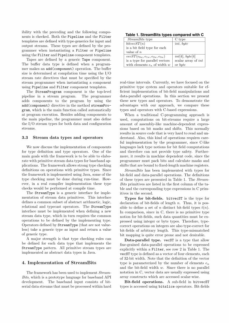
ibility with the preceding and the following compo-nents is checked. Both the Pipeline and the Filtertemplates are defined with type-generics for input andoutput streams. These types are defined by the pro-grammer when instantiating a Filter or Pipelineusing the Filter and Pipeline component templates.
Tapes are defined by a generic Tape component.The buffer data type is defined when a program-mer makes an add(component) operation. The buffersize is determined at compilation time using the I/Ostream rate directives that must be specified by thestream programmer when instantiating a componentusing Pipeline and Filter component templates.
The StreamProgram component is the top-levelpipeline in a stream program. The programmeradds components to the program by using theadd(component) directive in the method streamPro-gram, which is the main function called automaticallyat program execution. Besides adding components tothe main pipeline, the programmer must also definethe I/O stream types for both data and configurationstreams.
3.3 Stream data types and operators
We now discuss the implementation of componentsfor type definition and type operators. One of themain goals with the framework is to be able to elabo-rate with primitive stream data types for baseband ap-plications. The framework allows strong type checkingdefinitions on operations with primitive types. Sincethe framework is implemented using Java, some of thetype checking must be done during run-time. How-ever, in a real compiler implementation these typechecks would be performed at compile time.
The StreamType is a generic interface for imple-mentation of stream data primitives. This interfacedefines a common subset of abstract arithmetic, logic,relational and typecast operators. The StreamTypeinterface must be implemented when defining a newstream data type, which in turn requires the commonoperations to be defined by the implementing type.Operators defined by StreamType (that are not value-less) take a generic type as input and return a valueof generic type.
A major strength is that type checking rules canbe defined for each data type that implements theStreamType pattern. All primitive stream types areimplemented as abstract data types in Java.
4. Implementation of StreamBits
The framework has been used to implement Stream-Bits, which is a prototype language for baseband APIdevelopment. The baseband input consists of bit-serial data streams that must be processed within hard
Table 1. StreamBits types compared with CStreamBits type C type
bitvecST (n) int, byteis a bit field type for eachvalue of n
vecST (e0w, e1w, e2w, e3w) int[4], byte[4]is a type for parallel vectors scalar array of intwith elements en of width w or byte
real-time intervals. Currently, we have focused on theprimitive type system and operators suitable for ef-ficient implementation of bit-field manipulations anddata-parallel operations. In this section we presentthese new types and operators. To demonstrate theadvantages with our approach, we compare thesetypes and operators with C-based expressions.
When a traditional C-programming approach isused, computations on bit-streams require a largeamount of assembly-like machine-dependent expres-sions based on bit masks and shifts. This normallyresults in source code that is very hard to read and un-derstand. Also, this kind of operations requires care-ful implementation by the programmer, since C-likelanguages lack type notions for bit field computationsand therefore can not provide type safety. Further-more, it results in machine dependent code, since theprogrammer must pack bits and calculate masks andshifts that are bound to fixed-length machine registers.
StreamBits has been implemented with types forbit-field and data-parallel operations. The definitionsof these types are presented in Table 1. The Stream-Bits primitives are listed in the first column of the ta-ble and the corresponding type expressions in C prim-itives in the second.
Types for bit-fields. bitvecST is the type fordeclaration of bit-fields of length n. Thus, it is pos-sible to define a set of n distinct bit-field types t(n).In comparison, since in C, there is no primitive typenotion for bit-fields, such data quantities must be ex-pressed using integer or byte types. Therefore, type-correct operations on integers are also type-correct forbit-fields of arbitrary length. This type-mismatchedbit mapping is quite error prone and not desirable.
Data-parallel type. vecST is a type that allowfine-grained data-parallel operations to be expressedexplicitly within a Filter, see row 2 in Table 1. ThevecST type is defined as a vector of four elements, eachof 32-bit width. Note that the definition of the vectortype is parameterized by the number of elements en
and the bit-field width w. Since there is no parallelnotation in C, vector data are usually expressed usingarray constructs which are accessed scalar-wise.
Bit-field operations. A sub-field in bitvecSTtypes is accessed using bitslice operators. Bit-fields

Table 2. StreamBits compared with CbitvecST oper. Corresponding C expr.
bitslice(m : n) (t & wm:0)
bitsliceL(m : n) (t & wm:0) � (w −m)
bitsliceR(m : n) (t & wm:0) � n
bitslicePack(m : n) N/A
lmerge(k : l, m : n) if l <= (m− n) :
((t & wk:l) � C1) | ((s & wm:n) � n)
if l > (m− n) :
((t & wk:l) � C2) | ((s & wm:n) � n)
of bitvecST type can also be merged using the lmergeoperator. In Table 2, we list these operators and, forcomparison, the corresponding C expressions. Bit-field upper and lower boundaries are annotated withk, m and l, n respectively. w is used for machine word-length, and bit masks of machine register length areannotated with wm:0, where m represents the upperboundary of the bit mask.
The bitslice operator is currently defined for twocases – unaligned and aligned bit-slicing. Unalignedbit-slicing is performed with the bitslice("m:n")operator, row 1 in the table. The operator bit-slice("m:n") produces a bitvecST with the samelength as the operand, where bits m through n arecopied from the corresponding bit-field in the operand,and the rest are set to 0.
Aligned bit-slicing is performed by the oper-ators bitsliceL("m:n"), bitsliceR("m:n") andbitslicePack("m:n") listed on rows 2 through 4.The bitsliceL("m:n") operator produces a bit-fieldcopy, like bitslice("m:n"), but the copied bit-field isaligned to the bitvecST(n) upper bound n. Similarly,the bitsliceR("m:n") operator produces a bit-fieldcopy aligned to the lower bound. The correspond-ing expressions in C, on rows 2 and 3, require logi-cal AND and a SHIFT operations. In comparison,the bitsliceL and bitsliceR operators allow thisoperation to be more compactly expressed than therequired C expression. Also, in the C expression forleft-aligned masking on row 2, it is assumed that theupper bound is equal to the word length. But, sincethe bitvecST(n) type is defined for bit-fields of lengthn, this is generally not the case. The alignment ofbitsliceL and bitsliceR values in StreamBits canbe handled automatically at compile time.
The bitslicePack produces a left-aligned bit-fieldcopy, just like the bitsliceL operator, but the resultis packed into a bitvecST(s) where the field length sis equal to the length of the copied bit-field (m− n).
The lmerge operator is used to merge twobitvecST bit-fields. The result is a bitvecST(s)where the length s is the sum of the two merged bit-field lengths (k − l + m − n). The first operand isaligned to the left of the second operand. A right-aligned merge can be achieved by simply switching the
Table 3. Operator comparison vecSTStreamBits oper. Corresponding C expression
vecslice(m : n) for i = 0 to 4{t[ei] & wm:n}vecsliceL(m : n) for i = 0 to 4{t[ei] & wm:n � (w −m)}vecsliceR(m : n) for i = 0 to 4{t[ei] & wm:n � n}lmerge(k : l, m : n) for i = 0 to 4{
if l <= (m− n) :
(t[ei] & wk:l) � C1 | (s[ei] & wm:0) � n
if l > (m− n) :
(t[ei] & wk:l) � C2 | (s[ei] & wm:0) � n
order of the operands. The corresponding C expres-sion requires at most 5 operations. The first operandshould be aligned to the left of the second, which re-quires either a left or a right shift, depending on if themasked bit-fields are overlapping or not (l <= (m−n)or l > (m − n)). This alignment is a shift constantspecified by the programmer (C1 and C2). Thus, theif cases are used only to mark two separate alignmentcases.
Data-parallel operations. Besides the basicarithmetic and logical operations, the vecST typealso supports bit-field operations, such as lmerge,vecslice, vecsliceL and vecsliceR, see Table 3.The lmerge operation is defined precisely as lmergefor bitvecST types. The merge is performed in par-allel for each of the vector elements and the result isof type vecST. In StreamBits, the maximum length ofan element merge is w.
The vecslice(m:n), vecsliceL(m:n) and vec-sliceR(m:n) operators are vector-parallel versions ofbitslice operators. Since there is no correspond-ing parallel notation in C, parallelism must be trans-formed into sequential expressions, typically usingloop constructs and scalar data arrays. This is illus-trated in the right part of Table 3. Few will argue thatit is a natural way of expressing application parallelism– to use sequential scalar constructs, which are thento be parallelized by a compiler that is only aware ofthe sequential constructs given by the programmer.
Some computations require scalar processing ofvecST elements. Scalar elements in vecST are accessedby getElement(ei) and setElement(ei, val) opera-tors, where ei is the element index of the vector andval is the value.
5. Experiments with 3G UMTS base-band functions
In order to demonstrate and evaluate the applica-bility of the StreamBits language, we have conductedexperiments with baseband functions. In this papertwo different implementation examples of one base-band function are presented – cyclic redundancy check(CRC) processing for a voice call service and for high

for(intST cnt;cnt.lt(len);cnt.Assign(cnt.incr())){1. if(cnt.mod(new intST(4)).eq(new intST(0))){2. out.Assign(temp);3. temp.Assign(peekD());4. r_tmp.Assign(temp);5. pushD(popD());6. }7. t.Assign(r.bitsliceR("31:24"));8. r.Assign(r.lmerge("23:0", r_tmp.bitsliceR("31:24")));9. r.Assign(r.XOR(table[crc_poly.getVal()][t.getVal()]));10. r_tmp = r_tmp.lshift(8);}
Figure 2. CRC implemented in StreamBits
bit-rate data services [13].CRC processing for voice services. Voice calls
are coded using an adaptive multi rate codec (AMR).The baseband data input constitutes three AMR en-coded bit-streams mapped onto separate transportchannels, A, B and C. Each stream constitutes codedspeech data of different importance to the quality ofa voice channel; the A bits are the most importantand the C bits the least. The channels are processedwith different baseband parameters; only the A chan-nel bits are transmitted with a CRC computed check-sum. The CRC implementation, shown in figure 2, isa table-driven algorithm which encodes a single trans-port channel (Note that this is a selected part andnot the complete CRC baseband function). The vari-ables, except for the loop counter, are all of bitvecSTtype. In each loop iteration, this algorithm encodeseight-bit long fields of the input stream. The inputbits are packed into a stream of bitvecST data type.Each bitvecST is 32 bits long, thus four iterations arerequired to process each bitvecST that is read fromthe input stream. Defined by the code within the ifclause, every fourth iteration a new bitvecST valueis read into a temporary input register (r tmp), whilethe previous one is pushed to the output stream.
On line 7, the next 8-bit field to be encoded is readfrom the encoder register r using the bitsliceR op-erator. On line 8, the MSB from the temporary inputregister r tmp is shifted into the LSB of the encoderregister r using bitslice and lmerge.
Finally, the lookup value is read from the table tobe XOR:ed (the division), with the encoder register,and the next 8-bit input in the temporary register isaligned to the MSB position for the next iteration.
CRC processing for high bit-rate data. Datatransmissions can be mapped using multiple transportblocks of equal size, mapped on multiple transportchannels. Since there are no data dependencies be-tween the transport blocks, multiple blocks can beprocessed in parallel using SIMD control.
The StreamBits code in Figure 3 represents a SIMDparallel implementation of the same encoding algo-rithm previously demonstrated for the AMR service.
for(intST cnt;cnt.lt(len);cnt.Assign(cnt.incr())){1: if(cnt.mod(new intST(4)).eq(new intST(0))){2: out.Assign(temp);3: temp.Assign(peekD());4: r_tmp.Assign(temp);5: pushD(popD());6: }7: t.Assign(r.vecslice("31:24"));8: r.Assign(r.lmerge("23:0", r_tmp, "31:24"));9: v0.Assign(table[poly.val()][t.getElement(0).val()]);10: v1.Assign(table[poly.val()][t.getElement(1).val()]);11: v2.Assign(table[poly.val()][t.getElement(2).val()]);12: v3.Assign(table[poly.val()][t.getElement(3).val()]);13: r.Assign(r.XOR(new vecST(v0, v1, v2, v3)));14: r_tmp.Assign(r_tmp.lshift(8));}
Figure 3. CRC processing for DATA
The cnt and v0-v3 variables are scalar variables ofintST type, and the other are of vecST type. Like inthe AMR example, the parallel encoder encodes 8 bitsof the input stream per iteration.
Each data item in the I/O streams constitutes a32-bit field of four simultaneous transport block in-put streams; one transport block stream per vectorelement. The parallel vecslice operator on line 7copies the next 8 bits of each vector element in theencoder register r, and stores them aligned with thelsb positions in the t vector. Each element in t consti-tutes the next lookup index for each bit-stream beingprocessed. On line 8, new input bits are shifted intothe encoding register by copying the MSB of the in-put vector register r tmp, which are merged with theremaining bits in the encoder register. Like for thebitslice operators, no machine dependent maskingand shifting needs to be expressed in the code.
The table look-ups performed on lines 9 through12 have to be expressed with scalar operations; onelook-up for each element. This is because the inputbit-fields in register t constitute arbitrary values fromthe four transport blocks and therefore it is not possi-ble to vectorize the look-up operation. However, thisdoes not mean that this portion of the code cannotbe executed in parallel. Finally, the scalar values withthe look-up values are vectorized and XOR:ed withthe encoder register on line 13, and the next inputbits to be shifted into the encoder register are shiftedto the msb positions in the temporary input register,r tmp.
6 Conclusions and future work
We have described a configurable framework to beused for experiments with stream programming devel-opment targeting embedded high-performance appli-cations, such as baseband processing in radio base sta-tions. A domain specific language prototype for base-band processing, called StreamBits, was implementedto demonstrate the use of the framework and to per-
form implementation experiments. We introducedstream constructs to be able to efficiently programdynamic reconfiguration of distributed processing pa-rameters. It was shown that the language has the po-tential to lead to more compact and efficient codes forbit-field and data-parallel computations, compared towhen typical von Neumann based languages, such asC are used. The primitive types in the language im-pose a programmer to explicitly express functions withinherent, fine-grained data parallelism. Moreover, itwas demonstrated how the primitive data-parallel vec-tor and bit-vector data types and operations can beused without exposing machine specific details suchas register word lengths. Another advantage with theintroduced primitive data types is the opportunity toperform strong type checking on low-level bit opera-tions.
Future work will be focused on the definition of atailored stream processing language for baseband APIdevelopment. This will be based on extended proto-type experiments using the configurable framework.The development will include the implementation ofa compiler framework for a parallel machine abstrac-tion, which can be applied for efficient mapping onparallel and reconfigurable, array structured proces-sors. To support efficiency, the language should offerparallel expressions. To support portability, the syn-tax should not allow machine-specific details in thecode.
Acknowledgment
The authors would like to thank Dr. Anders Wassat Ericsson AB and Dr. Veronica Gaspes at HalmstadUniversity for valuable advice and suggestions. Thiswork has been funded by research grants from EricssonAB and the Knowledge Foundation.
References
[1] Freescale Semiconductor. MRC6011: Re-configurable Compute Fabric (RCF) Device.www.freescale.com, Oct. 2004.
[2] G. Panesar A. Duller and D. Towner. ParallelProcessing - the picoChip way! In Proc. of Com-municating Process Architectures, pages 125–138,2003.
[3] PACT XPP Technologies. XPP-IIb CoreOverview. www.pactcorp.com, Sept. 2005.
[4] H. Holma and A. Toskala. WCDMA for UMTS:Radio Access for Third Generation Mobile Com-munications. Addison-Wesley, third edition,2004.
[5] J. Lerzer Z. Zhang, F. Heiser and H. Leuschner.Advanced baseband technology in third-generation radio base stations. Ericsson Review,(01):32–41, 2003.
[6] M. B. Taylor et al. Evaluation of the Raw Micro-processor: An Exposed-Wire-Delay Architecturefor ILP and Streams. In Proc. of Int. Symposiumon Computer Architecture, pages 2–13, 2004.
[7] J. H. Ahn et al. Evaluating the Imagine StreamArchitecture. In Proc. of Int. Symposium onComputer Architecture, pages 14–25, 2004.
[8] A. E. Eichenberger et al. Optimizing Compilerfor a CELL Processor. In Proc. of Int. Conf.on Parallel Architectures and Compiation Tech-niques, pages 161–172, 2005.
[9] A. Das et al. Imagine Programming SystemUser’s Guide. www.cva.stanford.edu/imagine,April 2004.
[10] PACT XPP Technologies. Programming XPP-IIb Systems. www.pactcorp.com, Sept. 2005.
[11] S. V. Rajopadhye. Dependence Analysis and Par-allelizing Transformations. In The Compiler De-sign Handbook, pages 329–372. CRC Press, 2002.
[12] M. I. Gordon et al. A Stream Compiler forCommunication-Exposed Architectures. In Proc.of Int. Conf. on Architectural Support for Pro-gramming Languages and Operating Systems,pages 291–303, 2002.
[13] J. Bengtsson. Baseband Processing in 3G UMTSRadio Base Stations. Technical Report IDE0629,Halmstad University, 2006.
[14] E. Gamma. Design Patterns: Elements ofReusable Object-Oriented Software. Addison-Wesley professional computing series. Addison-Wesley, 1995.
Paper DA Domain-specific Approach for Software Development on
Manycore Platforms
Bengtsson, J. and Svensson, B. (2008). A domain-specific approach for soft-
ware development on manycore platforms. In ACM Computer ArchitectureNews, Special Issue: MCC08 - Multicore Computing 2008, 39(6):2-10.


A Domain-specific Approach for Software Development on Manycore Platforms
Jerker Bengtsson and Bertil SvenssonCentre for Research on Embedded Systems
Halmstad UniversityPO Box 823, SE-301 18 Halmstad, Sweden
Abstract
The programming complexity of increasingly parallelprocessors calls for new tools that assist programmers inutilising the parallel hardware resources. In this paper wepresent a set of models that we have developed as part of atool for mapping dataflow graphs onto manycores. One ofthe models captures the essentials of manycores identifiedas suitable for signal processing, and which we use as tar-get for our algorithms. As an intermediate representationwe introduce timed configuration graphs, which describethe mapping of a model of an application onto a machinemodel. Moreover, we show how a timed configuration graphby very simple means can be evaluated using an abstractinterpretation to obtain performance feedback. This infor-mation can be used by our tool and by the programmer inorder to discover improved mappings.
1. Introduction
To be able to handle the rapidly increasing programmingcomplexity of manycore processors, we argue thatdomainspecific development tools are needed. The signal process-ing required in radio base stations (RBS), see figure 1, isnaturally highly parallel and described by computations onstreams of data [9]. Each module in the figure encapsulatesa set of functions, further exposing more pipeline-, data-and task level parallelism as a function of the number ofconnected users. Many radio channels have to be processedconcurrently, each including fast and adaptive coding anddecoding of digital signals. Hard real-time constraints im-ply that parallel hardware, including processors and accel-erators is a prerequisite for coping with these tasks in a sat-isfactory manner.
One candidate technology for building baseband plat-forms is manycores. However, there are many issues thathave to be solved regarding development of complex signalprocessing software for manycore hardware. One such is
Radio RX Receiver
filter AGC
Remove prefix
FFT Extract user #1
Extract user #2
Extract user #2
Extract user #N
Demodulate Decode
Demodulate
Demodulate
Demodulate
Decode
Decode
Decode
User data
User data
User data
User data
Scheduler
Figure 1. A simplified modular view of theprincipal functions of the baseband receiverin long term evolution (LTE) RBS.
the need for tools that reduce the programming complexityand abstract the hardware details of a particular manycoreprocessor. We believe that if industry is to adopt manycoretechnologythe application software, the tools and the pro-gramming models need to be portable.
Research has produced efficient compiler heuristics forprogramming languages based on streaming models ofcomputation (MoC), achieving good speedup and highthroughput for parallel benchmarks [3]. However, eventhough a compiler can generate optimized code the pro-grammer is left with very little control of how the sourceprogram is transformed and mapped on the cores. Thismeans that if the resulting code output does not complywith the system timing requirements, the only choice is totry to restructure the source program. We argue thatexperi-enced application programmers must be able to direct andspecialize the parallel mapping strategy by giving directivetool input.
For complex real-time systems, such as basebandprocessing platforms, we see a need for tunable codeparallelization- and mapping tools, allowing programmersto take the system’s real-time properties into account dur-ing the optimization process. Therefore, complementary to

fully automatized parallel compilers, we are proposing aniterative code parallelization- and mapping tool flow thatallows the programmer to tune mapping by:
• analyzing the result of a parallel code map using per-formance feedback
• giving timing constraints, clustering and core alloca-tion directives as input to the tool
In our work we address the design and constructionof one such tool. We focus on suitable well defineddataflow models of computation for modeling applicationsand manycore targets, as well as the base for our intermedi-ate representation for manycore code-generation. One suchmodel, synchronous dataflow (SDF), is very suitable for de-scribing signal processing flows. It is also a good source forcode-generation, given that it has a natural form of paral-lelism that is a good match to manycores. The goal of ourwork is a tool chain that allows the software developer tospecify a manycore architecture (using ourmachine model),to describe the application (using SDF) and to obtain a gen-erated mapping that can be evaluated (using ourtimed con-figuration graph). Such a tool allows the programmer toexplore the run time behaviour of the system and to findsuccessively better mappings. We believe that this iterative,machine assisted, workflow, is good in order to keep the ap-plication portable while being able to make trade-offs con-cerning throughput, latency and compliance with real-timeconstraint on different platforms.
In this paper we present our set of models and show howwe can analyze the mapping of an application onto a many-core. More specifically, the contributions of this paper areas follows:
• A parallel machine model usable for modelling array-structured, tightly coupled manycore processors. Themodel is presented in Section 2, and in Section 3 wedemonstrate modeling of one target processor.
• A graph-based intermediate representation (IR), usedto describe a mapping of an application on a particu-lar manycore in the form of a (a timed configurationgraph). The use of this IR is twofold. We can performan abstract interpretation that gives us feedback aboutthe dynamic behaviour of the system. Also, we can useit to generate target code. We present the IR in Section4.
• We show in Section 5 how parallel performance can beevaluated through abstract interpretation of the timedconfiguration graph. As a proof of concept we haveimplemented our interpreter in the Ptolemy II softwareframework using dataflow process networks.
We conclude our paper with a discussion of our achieve-ments and future work.
2 Model Set
In this section we present the model set for constructingtimed configuration graphs. First we discuss the applicationmodel, which describes the application processing require-ments, and then the machine model, which is used to de-scribe computational resources and performance of many-core targets.
2.1 Application Model
We model an application using SDF, which is a specialcase of a computation graph [5]. An SDF graph constitutesa network of actors - atomic or composite of variable gran-ularity - which asynchronously compute on data distributedvia synchronous uni-directional channels. By definition, ac-tors in an SDF graph fire (compute) in parallel when thereare enough tokens available on the input channels. An SDFgraph is computable if there exists at least one static rep-etition schedule. A repetition schedule specifies in whichorder and how many times each actor is fired. If a repeti-tion schedule exists, buffer boundedness and deadlock freeexecution is guaranteed. A more detailed description of theproperties of SDF and how repetition schedules are calcu-lated can be found in [6].
The Ptolemy II modelling software provides an excel-lent framework for implementing SDF evaluation- and codegenerator tools [1]. We can very well consider an applica-tion model as an executable specification. For our work, itis not the correctness of the implementation that is in focus.We are interested in analyzing the dynamic, non-functionalbehaviour of the system. For this we rely on measures likeworst case execution time, size of dataflows, memory re-quirements etc. We assume that these data have been col-lected for each of the actors in the SDF graph and are givenas a tuple
< rp, rm, Rs, Rr >
where
• rp is the worst case computation time, in number ofoperations.
• rm is the requirement on local data allocation, inwords.
• Rs = [rs1, rs2
, ..., rsn] is a sequence wherersi
is thenumber of words produced on channeli each firing.
• Rr = [rr1, rr2
, ..., rrm] is a sequencerrj
is the numberof words consumed on channelj each firing.

2.2 Machine Model
One of the early, reasonably realistic, models for dis-tributed memory multiprocessors, is the LogP model [2].Work has been done to to refine this model, for exampletaking into account hardware support for long messaging,and to capture memory hierarchies. A more recent paral-lel machine model for multicores, which considers differentcore granularities and requirements on on-chip and off-chipcommunication is Simplefit [7]. However, this model wasderived with the purpose of exploring optimal grain size andbalance between memory, processing, communication andglobal I/O, given a VLSI budget and a set of computationproblems. Since it is not intended for modeling dynamicbehaviour of a program, it does not include a fine-granularmodel of the communication. Taylor et al. propose a tax-onomy (AsTrO) for comparison of scalar operand networks[11]. They also provide a tuple based model for comparingand evaluating performance sensitivity of on-chip networkproperties.
We propose a manycore machine model based on Sim-plefit and the AsTrO taxonomy, which allows a fairly fine-grained modeling of parallel computation performance in-cluding the overhead of operations associated with commu-nication. The machine model comprises a set of parametersdescribing the computational resources and a set of abstractperformance functions, which describe the computationalperformance of computations, communication and memorytransactions. We will later show in Section 5 how we cancan model dynamic, non-functional behavior of a dataflowgraph mapped on a manycore target, by incorporating themachine model in a dataflow process network.
2.2.1 Machine Specification
We assume that cores are connected in a mesh structurednetwork. Further that each core has individual instructiondecoding capability and software managed memory loadand store functionality, to replace the contents of core lo-cal memory. We describe the resources of such a manycorearchitecture using two tuples,M andF . M consists of a setof parameters describing the processors resources:
M =< (x, y), p, bg, gw, gr, o, so, sl, c, hl, rl, ro >
where
• (x, y) is the number of rows and columns of cores.
• p is the processing power (instruction throughput) ofeach core, inoperations per clock cycle.
• bg is global memory bandwidth, inwords per clockcycle
• gw is the penalty for global memory write, inwordsper clock cycle
• gr is the penalty for global memory read, inwords perclock cycle
• o is software overhead for initiation of a network trans-fer, in clock cycles
• so is core send occupancy, inclock cycles, when send-ing a message.
• sl is the latency for a sent message to reach the net-work, in clock cycles
• c is the bandwidth of each interconnection link, inwords per clock cycle.
• hl is network hop latency, inclock cycles.
• rl is the latency from network to receiving core, inclock cycles.
• ro is core receive occupancy, inclock cycles, when re-ceiving a message
F is a set of abstract functions describing the performanceof computations, global memory transactions and localcommunication:
F (M) =< tp, ts, tr, tc, tgw, tgr >
where
• tp is a function evaluating the time to compute a list ofinstructions
• ts is a function evaluating the core occupancy whensending a data stream
• tr is a function evaluating the core occupancy whenreceiving a data stream
• tc is a function evaluating network propagation delayfor a data stream
• tgw is a function evaluating the time for writing astream to global memory
• tgr is a function evaluating the time for reading astream from global memory
A specifc manycore processor is modeled by giving val-ues to the parameters ofM and by defining the functionsF (M).
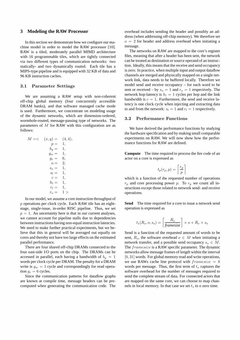
3 Modeling the RAW Processor
In this section we demonstrate how we configure our ma-chine model in order to model the RAW processor [10].RAW is a tiled, moderately parallel MIMD architecturewith 16 programmable tiles, which are tightly connectedvia two different types of communication networks: twostatically- and two dynamically routed. Each tile has aMIPS-type pipeline and is equipped with 32 KB of data and96 KB instruction caches.
3.1 Parameter Settings
We are assuming a RAW setup with non-coherentoff-chip global memory (four concurrently accessibleDRAM banks), and that software managed cache modeis used. Furthermore, we concentrate on modeling usageof the dynamic networks, which are dimension-ordered,wormhole-routed, message-passing type of networks. Theparameters ofM for RAW with this configuration are asfollows:
M =< (x, y) = (4, 4),p = 1,
bg = 1,
gw = 1,
gr = 6,
o = 2,
so = 1,
sl = 1,
c = 1,
hl = 1,
rl = 1,
ro = 1 >
In our model, we assume a core instruction throughput ofp operations per clock cycle. Each RAW tile has an eight-stage, single-issue, in-order RISC pipeline. Thus, we setp = 1. An uncertainty here is that in our current analyses,we cannot account for pipeline stalls due to dependenciesbetween instructions having non-equal instruction latencies.We need to make further practical experiments, but we be-lieve that this in general will be averaged out equally oncores and thereby not have too large effects on the estimatedparallel performance.
There are four shared off-chip DRAMs connected to thefour east-side I/O ports on the chip. The DRAMs can beaccessed in parallel, each having a bandwidth ofbg = 1words per clock cycle per DRAM. The penalty for a DRAMwrite is gw = 1 cycle and correspondingly for read opera-tion gr = 6 cycles.
Since the communication patterns for dataflow graphsare known at compile time, message headers can be pre-computed when generating the communication code. The
overhead includes sending the header and possibly an ad-dress (when addressing off-chip memory). We therefore seto = 2 for header and address overhead when initiating amessage.
The networks on RAW are mapped to the core’s registerfiles, meaning that after a header has been sent, the networkcan be treated as destination or source operand of an instruc-tion. Ideally, this means that the receive and send occupancyis zero. In practice, when multiple input and output dataflowchannels are merged and physically mapped on a single net-work link, data needs to be buffered locally. Therefore wemodel send and receive occupancy – for each word to besent or received – byso = 1 andro = 1 respectively. Thenetwork hop-latency ishl = 1 cycles per hop and the linkbandwidth isc = 1. Furthermore, the send and receive la-tency is one clock cycle when injecting and extracting datato and from the network:sl = 1 andrl = 1 respectively.
3.2 Performance Functions
We have derived the performance functions by studyingthe hardware specification and by making small comparableexperiments on RAW. We will now show how the perfor-mance functions for RAW are defined.
Compute The time required to process the fire code of anactor on a core is expressed as
tp(rp, p) =
⌈
rp
p
⌉
which is a function of the requested number of operationsrp and core processing powerp. To rp we count all in-structions except those related to network send- and receiveoperations.
Send The time required for a core to issue a network sendoperation is expressed as
ts(Rs, o, so) =
⌈
Rs
framesize
⌉
× o + Rs × so
Send is a function of the requested amount of words to besent,Rs, the software overheado ∈ M when initiating anetwork transfer, and a possible send occupancyso ∈ M .Theframesize is a RAW specific parameter. The dynamicnetworks allow message frames of length within the interval[0, 31] words. For global memory read and write operations,we use RAWs cache line protocol withframesize = 8words per message. Thus, the first term ofts captures thesoftware overhead for the number of messages required tosend the complete stream of data. For connected actors thatare mapped on the same core, we can choose to map chan-nels in local memory. In that case we setts to o zero time.

Receive The time required for a core to issue a networkreceive operation is expressed as
tr(Rr, o, ro) =
⌈
Rr
framesize
⌉
× o + Rr × ro
The receive overhead is calculated in a similar way as thesend overhead, except that parameters of the receiving corereplace the parameters of the sending core.
Network Propagation Time Modeling shared resourcesaccurately with respect to contention effects is very difficult.Currently, we assume that SDF graphs are mapped so thatthe communication will suffer from no or a minimum ofcontention. In the network propagation time, we considera possible network injection- and extraction latency at thesource and destination as well as the link propagation time.The propagation time is expressed as
tc(Rs, d, sl, hl, rl) = sl + d × hl + nturns + rl
Network injection- and extraction latency is captured bysl andrl respectively. Further, the propagation time is de-pendent on the network hop latencyhl and the number ofnetwork hopsd, which are determined from the source anddestination coordinates as|xs − xd| + |ys − yd|. Routingturns add an extra cost of one clock cycle. This is capturedby the value ofnturns which, similar tod, is calculated us-ing the source and destination coordinates.
Streamed Global Memory Read Reading from globalmemory on the RAW machine requires first one send op-eration (the core overhead which is captured byts), in or-der to configure the DRAM controller and set the address ofmemory to be read. The second step is to issue a receive op-eration to receive the memory contents on that address. Thepropagation time when streaming data from global memoryto the receiving core is expressed as
tgr = rl + d × hl + nturns
Note that memory read penalty is not included in thisexpression. This is accounted for in the memory model in-cluded in the IR. This is further discussed in Section 4
Streamed Global Memory Write Similarly to the mem-ory read operation, writing to global memory require twosend operations: one for configuring the DRAM controller(set write mode and address) and one for sending the datato be stored. The time required for streaming data from thesending core to global memory is evaluated by
tgw = sl + d × hl + nturns
Like in stream memory read, the memory write penaltyis accounted for in the memory model.
4 Timed Configuration Graphs
In this section we describe our manycore intermediaterepresentation (IR). We call the IR atimed configurationgraphbecause the usage of the IR is twofold:
• Firstly, the IR is a graph representing an SDF applica-tion graph, after it has been clustered and partitionedfor a specific manycore target. We can use the IR asinput to a code generator, in order to configure eachcore as well as the interconnection network and planglobal memory usage of a specific manycore target.
• Secondly, by introducing the notion of time in thegraph, we can use the same IR as input to an abstractinterpreter, in order to evaluate the dynamic behaviourof the application when executed on a specific many-core target. The output of the evaluator can be used ei-ther directly by the programmer or to extract informa-tion feedback to the tool for suggesting a better map-ping.
4.1 Relations Between Models and Con-figuration Graphs
A configuration graphGAM (V, E) describes an applica-
tion A mapped on the abstract machineM . The set of ver-ticesV = P∪B consists of coresp ∈ P and global memorybuffersb ∈ B. Edgese ∈ E represent dataflow channelsmapped onto the interconnection network. To obtain aGA
M ,the SDF forA is partitioned into subgraphs and each sub-graph is assigned to a core inM . The edges of the SDF thatend up in one subgraph are implemented using local mem-ory in the core, so they do not appear as edges inGA
M . Theedges of the SDF that reach between subgraphs can be dealtwith in two different ways:
1. A network connection between the two cores is usedand this appears as an edge inGA
M
2. Global memory is used as a buffer. In this case, a ver-tex b (and associated input- and output edges) is intro-duced between the two cores inGA
M .
WhenGAM has been constructed, eachv ∈ V ande ∈ E
has been assigned computation times and communicationdelays, calculated using the parameters ofM and the per-formance functionsF (M) introduced in Section 2.2. Theseannotations reflect the performance when computing the ap-plicationA on the machineM . We will now discuss howwe useA andM to configure the vertices, edges and thencomputational delays ofGA
M .

4.1.1 Vertices.
We distinguish between two types of vertices inGAM : mem-
ory vertices andcorevertices. Introducingmemoryverticesallows us to represent global memory. Amemoryvertex canbe specified by the programmer, for example to store ini-tial data. More typically,memoryvertices are automaticallygenerated when mapping channel buffers in global memory.
For core vertices, we abstract the firing of an actor bymeans of a sequenceS of abstractreceive, computeandsendoperations:
S = tr1, tr2
. . . trn, tp, ts1
, ts2, . . . , tsm
Thereceiveoperation has a delay corresponding to the tim-ing expressiontr, representing the time for an actor to re-ceive data through a channel. The delay of acomputeoper-ation corresponds to the timing expressiontp, representingthe time required to execute the computations of an actorwhen it fires. Finally, thesendoperation has a delay corre-sponding to the timing expressionts, representing the timefor an actor to send data through a channel.
For amemorytype of vertex, we assign delays specifiedby gr andgw in the machine model to account for memoryread- and write latencies respectively.
When buildingGAM , multiple channels sharing the same
source and destination can be merged and represented bya single edge, treating them as a single block or stream ofdata. Thus, there is always only one edgeei,j connectingthe pair(vi, vj). We add onereceiveoperation and onesendoperation to the sequenceS for each input and output edgerespectively.
4.1.2 Edges.
Edges represent dataflow channels mapped onto the inter-connection network. The weightw of an edgeei,j corre-sponds to the communication delay between vertexvi andvertexvj . The weightw depends on whether we map thechannel as a point-to-point data stream over the network, orin shared memory using amemoryvertex.
In the first case we assign the edge a weight correspond-ing totc. When a channel buffer is placed in global memory,we substitute the edge inA by a pair of input- and outputedges connected to amemoryactor. We illustrate this byFigure 2. We assign a delay oftgr andtgw to the input andoutput edges of thememoryvertex.
Figure 3 shows an example of a simpleA transformedto one possibleGA
M . A repetition schedule forA in thisexample is3(2ABCD)E. The repetition schedule shouldbe interpreted as: actorA fires 6 times, actorsB, C andD fire 3 times, and actorE 1 time. The firing ofA is re-peated indefinitly by this schedule. We use dashed lines foractors ofA mapped and translated toS inside each core ver-tex of GA
M . The feedback channel from C to B is mapped
A B
BM
gw grA
e1
e2
e3
w=tgw w=tgr
tstr
Figure 2. The lower graph ( GAM ) in the fig-
ure illustrates how the unmapped channel e1,connecting actor A and actor B, in the up-per graph ( A), has been transformed and re-placed by a global memory actor and edgese2 and e3.
A
B C
E
2
D
20
4
40
1 1
20 20
3
9
15
5
6A 3B 3C
E3D
12 12
120
120
9 9
15
15
120
120
Figure 3. The graph to the right is one possi-ble GA
M for the graph A to the left.
in local memory. The edge from A to D is mapped via aglobal buffer and the others are mapped as point-to-pointdata streams. The integer values represent the send andreceive rates of the channels (rs andrr), before and afterA has been clustered and transformed toGA
M , respectively.Note that these values inGA
M are the values inA multipliedby the number of the repetition schedule.
5 Interpretation of Timed ConfigurationGraphs
In this section we show how we can make an abstractinterpretation of the IR and how an interpreter can be im-plemented by very simple means on top of a dataflow pro-cess network. We have implemented such an interpreter us-ing the dataflow process networks (PN) domain in Ptolemy.The PN domain in Ptolemy is a super set of the SDF do-main. The main difference in PN, compared to SDF, is thatPN processes fire asynchronously. If a process tries to readfrom an empty channel, it will block until there is new dataavailable. The PN domain implemented in Ptolemy is a spe-cial case of Kahn process networks [4]. Unlike in a Kahnprocess network, PN channels have bounded buffer capac-ity, which implies that a process also temporarily blocks
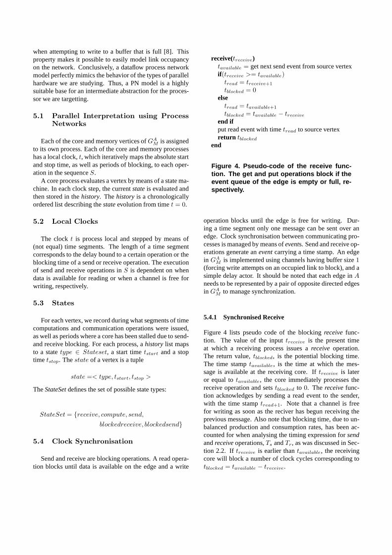
when attempting to write to a buffer that is full [8]. Thisproperty makes it possible to easily model link occupancyon the network. Conclusively, a dataflow process networkmodel perfectly mimics the behavior of the types of parallelhardware we are studying. Thus, a PN model is a highlysuitable base for an intermediate abstraction for the proces-sor we are targetting.
5.1 Parallel Interpretation using ProcessNetworks
Each of the core and memory vertices ofGAM is assigned
to its own process. Each of the core and memory processeshas a local clock,t, which iteratively maps the absolute startand stop time, as well as periods of blocking, to each oper-ation in the sequenceS.
A core process evaluates a vertex by means of a state ma-chine. In each clock step, the currentstateis evaluated andthen stored in thehistory. Thehistory is a chronologicallyordered list describing thestateevolution from timet = 0.
5.2 Local Clocks
The clockt is process local and stepped by means of(not equal) time segments. The length of a time segmentcorresponds to the delay bound to a certain operation or theblocking time of a send or receive operation. The executionof send and receive operations inS is dependent on whendata is available for reading or when a channel is free forwriting, respectively.
5.3 States
For each vertex, we record during what segments of timecomputations and communication operations were issued,as well as periods where a core has been stalled due to send-and receive blocking. For each process, ahistory list mapsto a statetype ∈ Stateset, a start timetstart and a stoptime tstop. Thestate of a vertex is a tuple
state =< type, tstart, tstop >
TheStateSetdefines the set of possible state types:
StateSet = {receive, compute, send,
blockedreceive, blockedsend}
5.4 Clock Synchronisation
Send and receive are blocking operations. A read opera-tion blocks until data is available on the edge and a write
receive(treceive)tavailable = get next send event from source vertexif(treceive >= tavailable)
tread = treceive+1
tblocked = 0else
tread = tavailable+1
tblocked = tavailable − treceive
end ifput read event with timetread to source vertexreturn tblocked
end
Figure 4. Pseudo-code of the receive func-tion. The get and put operations block if theevent queue of the edge is empty or full, re-spectively.
operation blocks until the edge is free for writing. Dur-ing a time segment only one message can be sent over anedge. Clock synchronisation between communicating pro-cesses is managed by means ofevents. Send and receive op-erations generate aneventcarrying a time stamp. An edgein GA
M is implemented using channels having buffer size1(forcing write attempts on an occupied link to block), and asimple delay actor. It should be noted that each edge inA
needs to be represented by a pair of opposite directed edgesin GA
M to manage synchronization.
5.4.1 Synchronised Receive
Figure 4 lists pseudo code of the blockingreceivefunc-tion. The value of the inputtreceive is the present timeat which a receiving process issues areceiveoperation.The return value,tblocked, is the potential blocking time.The time stamptavailable, is the time at which the mes-sage is available at the receiving core. Iftreceive is lateror equal totavailable, the core immediately processes thereceive operation and setstblocked to 0. The receivefunc-tion acknowledges by sending a read event to the sender,with the time stamptread+1. Note that a channel is freefor writing as soon as the reciver has begun receiving theprevious message. Also note that blocking time, due to un-balanced production and consumption rates, has been ac-counted for when analysing the timing expression forsendandreceiveoperations,Ts andTr, as was discussed in Sec-tion 2.2. If treceive is earlier thantavailable, the receivingcore will block a number of clock cycles corresponding totblocked = tavailable − treceive.

5.4.2 Synchronised Send
Figure 5 lists pseudo code for the blockingsendfunction.The value oftsend is the time at which thesendoperationwas issued. The time stamp of the read eventtavailable cor-responds to the time at which the receiving vertex reads theprevious message and thereby also when the edge is avail-able for sending next message. Iftsend < tavailable, asendoperation will block fortblocked = tavailable − tsend clockcycles. Otherwisetblocked is set to0. Note that all edgescarrying receive events in theconfiguration graphmust beinitialised with a read event, otherwise interpretation willdeadlock.
send(tsend)tavailable = get read event from sink vertexif(tsend < tavailable)
tblocked = tavailable − tsend
elsetblocked = 0
end ifput send eventtsend + ∆e + tblocked to sink vertexreturn tblocked
end
Figure 5. Pseudo-code of the send function.The value of ∆e corresponds to the delay ofthe edge.
5.5 Vertex Interpretation
Figure 6 lists the pseudo code for interpretation of avertex inGA
M . It should be noted that, for space reasons,we have omitted to include the state code for global readand write operations. The functioninterpretV ertex() isfinitely iterated by each process and the number of itera-tions, iterations, is equally set for all vertices when pro-cesses are initated. Each process has a local clockt and anoperation counterop cnt, both initially set to0. The opera-tions sequenceS is a process local data structure, obtainedfrom the vertex to be interpreted. Furthermore, each pro-cess has a listhistory which initially is empty. Also, eachprocess has a variablecurr oper which holds the currentlyprocessed operation inS.
The vertex interpreter makes state transitions dependingon the current operationcurr oper, the associated delayand whethersendandreceiveoperations block or not. Asdiscussed in Section 5.4.1, thesendand receivefunctionsare the only blocking functions that can halt the interpre-tation in order to synchronise the clocks of the processes.
The value oftblocked is set to the return value ofsendandreceivewhen interpreting send and receive operations, re-spectively. The value oftblocked corresponds to the length oftime asendor receiveoperation was blocked. Iftblocked hasa value> 0, a state of typeblockedsendor blockedreceiveis computed and added to thehistory.
interpretVertex()if (list S has elements)
while(iterations > 0)get elementop cnt in S and put incurr oper
incrementop cnt
if(curr op is a Receive operation)settblocked = value ofreceive(t)if(tblocked > 0)
add state ReceiveBlocked(t, tblocked) to hist.
sett = t + tblocked
end ifadd state Receiving(t, ∆ of curr oper)
end if
else if(curr op is a Compute operation)add state Computing(t, ∆ of curr oper)
end if
else if(curr op is a Send operation)settblocked = value ofsend(t)if(tblocked > 0)
add state SendBlocked(t, tblocked) to hist.
sett = t + tblocked
end ifadd state Sending(t, ∆ of curr oper)
end if
if(op cnt reached last index ofS)setop cnt = 0decrementiterations
add stateEnd(t) to history
end ifsett = t + ∆ of curr oper + 1
end whileend if
end
Figure 6. Pseudo-code of the interpretVertexfunction.

5.6 Model Calibration
We have implemented the abstract interpreter in thePtolemy software modeling framework [1]. Currently, wehave verified the correctness of the interpreter using a setof simple parallel computation problems from the literature.Regarding the accuracy of the model set, we have so far onlycompared the performance functions separately against cor-responding operations on RAW. However, to evaluate andpossibly tune the model for higher accuracy we need to dofurther experimental tests with different relevant signalpro-cessing benchmarks, especially including some more com-plex communication- and memory access patterns.
6 Discussion
We believe that tools supporting iterative mapping andtuning of parallel programs on manycore processors willplay a crucial role in order to maximise application per-formance for different optimization criteria, as well as toreduce the parallel programming complexity. We also be-lieve that using well defined parallel models of computa-tion, matching the application, is of high importance in thismatter.
In this paper we have presented our achievements to-wards the building of an iterative manycore code generationtool. We have proposed a machine model, which abstractsthe hardware details of a specific manycore and providesa fine-grained instrument for evaluation of parallel perfor-mance. Furthermore, we have introduced and describedan intermediate representation calledtimed configurationgraph. Such a graph is annotated with computational delaysthat reflect the performance when the graph is executed onthe manycore target. We have demonstrated how we com-pute these delays using the performance functions includedin the machine model and the computational requirementscaptured in the application model. Moreover, we have indetail demonstrated how performance of atimed configura-tion graphcan be evaluated using abstract interpretation.
As part of future work, we need to perform furtherbenchmarking experiments in order to better determine theaccuracy of our machine model compared to chosen targetprocessors. Also, we have so far builttimed configurationgraphs by hand. We are especially interested in exploringtuning methods, using feedback information from the eval-uator to set constraints in order to direct and improve themapping of application graphs. Currently we are workingon automatising the generation of thetimed configurationgraphs in our tool-chain, implemented in the Ptolemy IIsoftware modelling framework.
Acknowledgment
The authors would like to thank Henrik Sahlin and PeterBrauer at the Baseband Research group at Ericsson AB, Dr.Veronica Gaspes at Halmstad University, and Prof. EdwardA. Lee and the Ptolemy group at UC Berkeley for valu-able input and suggestions. This work has been funded byresearch grants from the Knowledge Foundation under theCERES contract.
References
[1] C. Brooks, E. A. Lee, X. Liu, S. Neuendorffer, Y. Zhao, andH. Zheng. Heterogeneous Concurrent Modeling and De-sign in Java (Volume 1: Introduction to Ptolemy II). Techni-cal Report UCB/EECS-2008-28, EECS Dept., University ofCalifornia, Berkeley, Apr 2008.
[2] D. Culler, R. Karp, and D. Patterson. LogP: Towards a Real-istic Model of Parallel Computation. InProc. of ACM SIG-PLAN Symposium on Principles and Practices of Parallelprogramming, May 1993.
[3] M. I. Gordon, W. Thies, and S. Amarasinghe. Exploit-ing Coarse-Grained Task, Data, and Pipeline Parallelism instream programs. InProc. of Twelfth Int’l. Conf. on Archi-tectural Support for Programming Languages and Operat-ing Systems, 2006.
[4] G. Kahn. The Semantics of a Simple Language for Paral-lel Programming. In J. L. Rosenfeld, editor,IFIP Congress74, pages 471–475, Stockholm, Sweden, August 5-10 1974.North-Holland Publishing Company.
[5] R. M. Karp and R. E. Miller. Properties of a Model for Par-allel Computations:Determinancy, Termination, Queueing.SIAM Journal of Applied Mathematics, 14(6):1390–1411,November 1966.
[6] E. A. Lee and D. G. Messerschmitt. Static Scheduling ofSynchronous Data Flow Programs for Signal Processing.IEEE Trans. on Computers, January 1987.
[7] C. A. Moritz, D. Yeung, and A. Agarwal. SimpleFit: AFramework for Analyzing Design Tradeoffs in Raw Archi-tectures.IEEE Trans. on Parallel and Distributed Systems,12(6), June 2001.
[8] T. M. Parks. Bounded Scheduling of Process Networks.PhD thesis, EECS Dept., University of California, Berkeley,Berkeley, CA, USA, 1995.
[9] H. Sahlin. Introduction and overview of LTE BasebandAlgorithms. Powerpoint presentation, Baseband researchgroup, Ericsson AB, February 2007.
[10] M. B. Taylor, J. Kim, J. Miller, D. Wentzlaff, F. Ghodrat,B. Greenwald, H. Hoffman, P. Johnson, J.-W. Lee, W. Lee,A. Ma, A. Saraf, M. Seneski, N. Shnidman, V. Strumpen,M. Frank, S. Amarasinghe, and A. Agarwal. The Raw Mi-croprocessor: A Computational Fabric for Software Circuitsand General-Purpose Programs.IEEE Micro, 22(2):25–35,2002.
[11] M. B. Taylor, W. Lee, S. P. Amarasinghe, and A. Agarwal.Scalar Operand Networks.IEEE Trans. on Parallel and Dis-tributed Systems, 16(2):145–162, 2005.


Paper EManycore Performance Analysis using Timed Configuration
Graphs
Bengtsson, J. and Svensson, B. (2009). Manycore performance analysis us-
ing timed configuration graphs. To appear in Proc of. Int’l Symp. on Sys-tems, Architectures, Modeling and Simulation (SAMOS IX 2009), Samos,
Greece.


Manycore Performance Analysis using TimedConfiguration Graphs
Jerker BengtssonCentre for Research on Embedded Systems
Halmstad UniversityHalmstad, Sweden
Email: [email protected]
Bertil SvenssonCentre for Research on Embedded Systems
Halmstad UniversityHalmstad, Sweden
Email: [email protected]
Abstract—The programming complexity of increasingly par-allel processors calls for new tools to assist programmers inutilising the parallel hardware resources. In this paper we presenta set of models that we have developed to form part of a toolwhich is intended for iteratively tuning the mapping of dataflowgraphs onto manycores. One of the models is used for capturingthe essentials of manycores that are identified as suitable forsignal processing and which we use as target architectures.Another model is the intermediate representation in the formof a timed configuration graph, describing the mapping of adataflow graph onto a machine model. Moreover, this IR can beused for performance evaluation using abstract interpretation.We demonstrate how the models can be configured and appliedin order to map applications on the Raw processor. Furthermore,we report promising results on the accuracy of performancepredictions produced by our tool. It is also demonstrated thatthe tool can be used to rank different mappings with respect tooptimisation on throughput and end-to-end latency.
I. INTRODUCTION
For efficient handling of the programming complexity ofmanycore processors, domain specific development tools areneeded. One concrete example is the signal processing re-quired in radio base stations (RBS), which is naturally highlyparallel and described by computations on streams of data [1].Many user channels have to be processed concurrently, eachincluding fast and adaptive coding and decoding of digitalsignals. Hard real-time constraints imply that parallel hard-ware, including processors and accelerators is a prerequisitefor coping with these tasks in a satisfactory manner.
One candidate technology for building flexible high-performance processing platforms is manycores. However,there are many issues regarding development of complexsignal processing software for manycore hardware. One such isthe need for tools that reduce the programming complexity andabstract hardware details of a particular manycore processor.We believe that, if industry is to adopt commercial-off-the-shelf (COTS) manycore technology, the application software,the tools and the programming models need to a high degreebe portable.
Research has produced specialised compiler techniques forprogramming languages based on streaming models of com-putation, achieving good speedup and high throughput forparallel benchmarks [2]. However, even though a compiler cangenerate optimised code, the programmer is typically left with
very little control of how the source program is transformedand mapped on the cores. This means that, if the code outputdoes not meet the non- functional requirements of the system,the only choice is to try to restructure the source program. Weargue that in order to increase performance gain experiencedapplication programmers must be able to control the parallelmapping strategy.
We are developing an iterative code mapping tool thatallows the programmer to tune a mapping by:
• analysing the result of a parallel mapping using inter-preted performance feedback
• giving timing, clustering and core allocation constraintsas input to the tool
Figure 1 outlines the modular architecture of our tool.The tool is designed for using well defined dataflow modelsof computation. One special case of dataflow, synchronousdataflow (SDF), is very suitable for describing signal process-ing flows [3]. It is also a good source for code generation toparallel hardware, because it has a natural form of parallelismthat is a good match to manycores. The programmer providesa manycore machine specification (using our machine model)and the program (using SDF) as input to the tool. Duringthe model analysis stage, the tool will analyse the processingrequirements of the SDF model. As the second stage, wecompute a static dataflow schedule for the SDF graph (giventhat the SDF model is consistent). The scheduled graphis then passed through a model transformation. During themodel transformation, the tool generates a timed intermediaterepresentation, which represents an abstract mapping of theapplication on a specific target processor. We call our inter-mediate representation a timed configuration graph.
In this paper we present our achievements on the modelsand the timed intermediate representation used by the tool tocompute performance feedback to the user. The interpretedperformance feedback enables a programmer to, early in thedevelopment process, explore the run time performance of thesoftware and to find successively better mappings. We believethat this iterative, machine assisted workflow, is advantageousin order to keep the application portable while being able tomake trade-offs concerning throughput, latency and compli-ance with real-time constraint on different platforms. More

Model Analysis
Dataflow Scheduling
Model Transformation
Abstract Interpretation
Code Generation
User feedback
Machine specification SDF
Manycoreconfiguration
(Timed IR)
Fig. 1. Outline of the manycore code mapping tool.
specifically, the contributions of this paper are as follows:• A parallel machine model usable for modelling array-
structured, tightly coupled manycore processors. Themodel is presented in Section III, and in Section V wedemonstrate the configuration of it for modelling the Rawprocessor[4].
• An intermediate representation (IR), used to describe amapping of an application on a particular manycore inthe form of a timed configuration graph. The use of thisIR is twofold: We can perform an abstract interpretationthat gives us feedback of performance during executionof the system. Also, we can use it to generate target code.We present the IR in Section IV.
• We make an evaluation of the accuracy and the usefulnessof our tool in Section VI. It is shown that our tool is ableto correctly rank different mappings of a graph by highestthroughput or shortest end-to-end latency.
We conclude the paper with a discussion of the results of theevaluation and we point to improvements in order to increasethe accuracy of some of the predictions.
II. RELATED WORK
The problem of mapping task graphs in the form of acyclicprecedence graphs (APG) to a parallel processor has been awidely addressed problem. Heuristic solutions are requiredsince this is for a long time known to be an NP completeproblem [5]. Sarkar introduced the two step mapping method,where clustering is performed in a first step independentlyfrom the second step of scheduling and processor allocation,which can be applied at compile time [6]. A number of leadingalgorithms, for both single step and two step clustering andmerging, with objectives of transforming and mapping taskgraphs for multiprocessor systems are reviewed in [7].
The dynamic level scheduling algorithm proposed by Sihand Lee is an heuristic taking inter-processor communicationoverhead into account during clustering. Similar to our work,this scheduling algorithm can be used to produce feedbackto the programmer for iterative refining of the task graphand the architecture [8]. However, it has been demonstrated
by Kianzad and Bhattacharyya that two step methods tend toproduce more qualitative schedules than single step methods[7]. Unfortunately, expanding an SDF graph to an acyclicprecedence graph – which are the assumed representation formany scheduling and mapping algorithms – can lead to anexplosion of nodes. This problem can partly be reduced usingclustering techniques before the SDF graph is transformed toan APG [9]. However, we are interested in techniques foranalysis and mapping of SDF graphs without conversion toan APG
The StreamIt language implements a restricted set of SDF.The StreamIt compiler implements a two phase mapping(dataflow scheduling and clustering, followed by core al-location) using direct representation of SDF graphs [2][4].However, the StreamIt compiler uses a static and location inde-pendent cost model for clustering and core allocation. Further,neither the language nor the compiler provides any means toexpress non-functional constraints or other application specificoptimisation criteria to tune the parallel mapping and codegeneration. Programs have to be restructured in attempts toimprove a mapping.
Throughput is one important non-functional requirement inthe real-time applications we are addressing. Ghamarian et al.provide methods for throughput using state space analysis ondirect representation of multi-rate SDF graphs [10]. Further,Stuijk et al. have developed a multiprocessor resource alloca-tion strategy for throughput constrained SDF graphs [11]. Weare addressing techniques that allow combinations of timingconstraints and show how to use them to direct the mappingprocess.
Bambha and Battacharyya provide a good review of dif-ferent intermediate representations for different objectives onoptimisation and synthesis for self-timed execution of SDFprograms to multiprocessor DSP systems [12]. They assumehomogenous representation of SDF graphs, which exposes ahigher degree of task parallelism based on the rate signatures.Our work is similar, but we are mainly interested intermediaterepresentations on multi-rate SDF and in minimising transfor-mation between different representations during the mappingprocess.
III. MODEL SET
In this section we present the model set for constructingtimed configuration graphs. First we discuss the applicationmodel, which describes the application processing require-ments, and then the machine model, which is used to describecomputational resources and performance of manycore targets.
A. Application Model
We model an application using multi-rate SDF. An SDFgraph constitutes a network of actors – atomic or compositeof variable granularity – which compute on data distributed viasynchronous unidirectional channels. Each channel input andoutput of an actor has an a priori specified token consumptionand production rate. By definition, memory and computationsin an SDF graph are distributed, and actors fire (compute)

in parallel when there are enough tokens available on theinput channels. An SDF graph is computable if there exists atleast one periodical repetition schedule. A periodical repetitionschedule specifies in which order and how many times eachactor fires. If a repetition schedule exists, buffer boundednessand deadlock free execution is guaranteed. One significantadvantage with SDF is that the execution order can be de-termined at compile-time. This enables generation of compactcode and elimination of run-time scheduling overhead [13].The properties of SDF and the formal theory for schedulingof SFD graphs are in detail described in [3].
The Ptolemy modelling framework provides an excellentbasis for implementing SDF analysis and code generationtools [14]. Besides serving as input to a code generator, theapplication model is an executable specification. However, forour work it is not the correctness or the functional properties ofthe application that is in focus. We are interested in techniquesfor analysing the non-functional properties of the system. Forthis we rely on measures like worst case execution time,communication and memory requirements. We assume thatthese data have been analysed and that each actor is associatedwith a tuple
< rp, rm, Rs, Rr >
where• rp is the worst case execution time, in number of opera-
tions.• rm is the requirement on memory allocation, in words.• Rs = [rs1 , rs2 , ..., rsn
] is a sequence where rsiis the
number of words produced on channel i each firing.• Rr = [rr1 , rr2 , ..., rrm
] is a sequence where rrjis the
number of words consumed on channel j each firing.
B. Machine Model
Scheduling and core allocation algorithms need to takeinter processor (core) communication into account to providerealistic cost measures. These costs in general comprise astatic cost for sending and receiving and a dynamic costdetermined by the resource location and/or the amount ofdata to be communicated. However, for reasonably near clock-cycle accurate modelling of dynamic network behaviour it isnecessary to use a fine grained cost model for communication.We discuss this further in conjunction with our experimentalresults in Section VI.
One well-studied and reasonably realistic model for dis-tributed memory multiprocessors is LogP [15]. During thepast, much work has been done to refine this model, for exam-ple taking into account hardware support for long messaging[16], and capturing network contention [17]. A more recentparallel machine model targeting fine-grained and large scalemulticores is developed as a part of the SimpleFit framework[18]. SimpleFit considers variable core granularities and re-quirements on on-chip and off-chip communication. However,it was derived with the purpose of exploring optimal grainsize and balance between memory, processing, communication
and global I/O, given a VLSI budget and a set of computationproblems. Since it is not intended for modelling the dynamicbehaviour of a program, it does not include a fine-granularmodel of the communication. Taylor et al. propose a taxonomy(AsTrO) for comparison of scalar operand networks [19]. Thistaxonomy includes a five parameter tuple for comparing andevaluating performance sensitivity of on-chip scalar operandnetworks.
We propose a manycore machine model based on SimpleFitand the AsTrO five parameter tuple. This model allows a fairlyfine-grained modelling of performance, including the overheadof operations associated with communication and off-chipresources. The machine model comprises a set of parametersdescribing the computational resources and a set of abstractperformance functions, which describe the performance ofcomputations, communication and memory transactions.
We assume that cores are tightly coupled via a meshnetwork. Further that each core has individual instruction se-quencing capability and that transactions between core privateand shared memory is software managed. The resources ofsuch an abstract manycore architecture are described using twotuples, M and F . M consists of a set of parameters describingthe resources:
M =< (x, y), p, bg, gw, gr, o, so, sl, c, hl, rl, ro >
where• (x, y) is the number of rows and columns of cores.• p is the processing power (instruction throughput) of each
core, in operations per clock cycle.• bg is global memory bandwidth, in words per clock cycle• gw is the penalty for global memory write, in words per
clock cycle• gr is the penalty for global memory read, in words per
clock cycle• o is software overhead for initiation of a network transfer,
in clock cycles• so is core send occupancy, in clock cycles, when sending
a message.• sl is the latency for a sent message to reach the network,
in clock cycles• c is the bandwidth of each interconnection link, in words
per clock cycle.• hl is network hop latency, in clock cycles.• rl is the latency from network to receiving core, in clock
cycles.• ro is core receive occupancy, in clock cycles, when
receiving a messageF is a set of abstract common functions describing theperformance of computations, global memory transactions andlocal communication as functions of M :
F (M) =< tp, ts, tr, tc, tgw, tgr >
where

• tp is a function evaluating the time to compute a sequenceof instructions
• ts is a function evaluating the core occupancy whensending a data stream
• tr is a function evaluating the core occupancy whenreceiving a data stream
• tc is a function evaluating network propagation delay fora data stream
• tgw is a function evaluating the time for writing a streamto global memory
• tgr is a function evaluating the time for reading a streamfrom global memory
A specific manycore processor is modelled by giving valuesto the parameters of M and by defining the functions F (M).
IV. MANYCORE INTERMEDIATE REPRESENTATION
In this section we describe the manycore intermediaterepresentation (IR). We call the IR a timed configuration graphbecause the usage of the IR is twofold:
• Firstly, the IR is a graph representing an SDF pro-gram that is transformed and partitioned for a specificmanycore target. We can use the IR as input to a codegenerator, in order to configure each core as well as theinterconnection network and plan global memory usageof a specific manycore target.
• Secondly, by introducing the notion of time in the graph,we can use the same IR as input to an abstract interpreter,in order to predict performance and evaluate the dynamicbehaviour of the application when executed on a specificmanycore target. The output of the evaluator can be usedeither directly by the programmer or by an auto-tuner forsuggesting a better mapping.
A. Relations Between Models and Configuration Graphs
A timed configuration graph GAM (V,E) describes a single
connected SDF graph A, transformed and mapped on theabstract machine described by the pair of tuples (M,F ). Theset of vertices is a union V = P∪B|P∩B = ∅, where P is theset of cores and B is the set of off-chip shared memories. Weuse vp to denote a vertex of core type and vb to denote a vertexof memory type. Edges e ∈ E are dataflow channels mappedonto the interconnection network of (M, F ). To obtain a GA
M ,the vertices of A are clustered with respect to the integrityof the dataflow. Each cluster is assigned to a core in M . Theedges of the SDF that end up in one cluster are implementedusing local memory in the core, so they do not appear as edgesin GA
M . The edges of the SDF that reach between clusters canbe implemented in two different ways:
1) as network connection between the two cores. Suchconnection is represented by an edge (vpi , vpj ) in GA
M
2) as a buffer in global memory. In this case, a vertex vbk
is introduced. Further the edge (vpi, vpj
) is replaced bya pair of edges (vpi
, vbk) and (vbk
, vpj) between the two
cores in GAM .
When GAM has been constructed, each vp, vb ∈ V has been
assigned costs for computation and communication, calculated
using the machine description (M, F ) described in SectionIII-B. These costs reflect the relative costs for each specificoperation when computing A on (M,F ). We will now discusshow we use A and M to construct and assign costs to thevertices, the edges and the computation costs of GA
M .1) Vertices.: Memory vertices, B, allow us to represent a
set of buffers mapped in shared memory. A memory vertex canbe specified by the programmer, for example to store initialdata. Memory vertices can also be automatically generated.
For core vertices, P , we abstract the firing of an actor bymeans of a sequence S of abstract receive, compute and sendoperations:
S = tr1 , tr2 . . . trn, tp, ts1 , ts2 , . . . , tsm
The cost for a receive operation depends on whether the sourceis another core or a shared memory. Let the source vertex ofchannel e be source(e). Then for each incoming edge of avertex p we add a receive operation with a cost bound to:
• tr ∈ F (M), if source(e) is of type vp
• tgr ∈ F (M), if source(e) is of type vb
The cost for a compute operation is calculated using theperformance function tp, which represents the time requiredto execute the computations of an actor when it fires.
Finally, for each outgoing edge of a vertex p we add a sendoperation. Let the sink vertex of channel e be sink(e). Thesend operation has a cost bound to:
• ts ∈ F (M), if sink(e) is of type vp
• tgw ∈ F (M), if sink(e) is of type vb
Read and write requests on memory vertices are served bythe first come first served policy. For a vertex vb we assignread and write costs calculated using gr ∈ M and gw ∈ M ,to account for memory read- and write latencies when servingan incoming request.
When constructing GAM , multiple channels sharing the same
source and destination can be orderly merged and representedby a single edge, treating them as a single stream of data.
2) Edges.: The weight w of an edge e(vi, vj) correspondsto the link propagation. The value of the weight w correspondsto the value of the function tc ∈ F (M). Further, edges in SDFcan be specified with a sample delay. Given an edge e(vi, vj),a unit delay is defined to mean that the nth sample consumedby vj corresponds to the (n−1)th sample produced by vertexvi [3]. An edge delay is simply represented by a buffer offsetvalue, needing no further treatment when constructing GA
M .Figure 2 shows an example of a simple SDF graph, A, after
it has been transformed to one possible GAM . One static firing
schedule for A in this example is 3(2abcd)e. The scheduleshould be interpreted as: actor a fires 6 times, actors b, c andd fire 3 times, and actor e 1 time. The firing of A is repeatedindefinitely by this schedule. Thus, no runtime schedulingsupervision is required. The feedback channel from actor cto actor b is buffered in core local memory. The edge fromactor a to actor d is a buffer in shared (off-chip) memory andthe others are mapped as point-to-point connections on thenetwork. The integer values represent the send and receive

a
b c
e
2
d20
4
40
1 1
20 20
39
155
6a 3b 3c
1e3d
12 12
120120
9 9
1515
120120
Fig. 2. The graph to the right is one possible graph GAM for the application
graph A to the left.
rates of the channels (rs and rr), before and after A has beenclustered and transformed to GA
M , respectively. Note that thesevalues in GA
M are the values in A multiplied by the numberof times an actor fires, as given by the firing schedule.
B. Interpretation of Timed Configuration Graphs
In order to implement and interpret timed configurationsgraphs, we need a computational model and a notion oftime [20]. We have used dataflow process network (PN) toimplement interpretable timed configuration graphs [21]. Aprocess network very well mimics the behaviour of the typesof parallel hardware we are studying. The PN domain inPtolemy is a super set of the SDF domain. The main differencein PN, compared to SDF, is that actors are processes whichfire asynchronously. If a process tries to read from an emptychannel, it will block until there is new data available. ThePN domain implemented in Ptolemy is a special case of Kahnprocess networks [22]. But, unlike in a Kahn process network,PN channels have bounded buffer capacity, which implies thata process also temporarily blocks when attempting to write toa buffer that is full. This property enables easy modelling oflink occupancy on the network.
Each of the core and memory vertices of GAM is assigned
to its own process. Each of the processes has a local clock,t, which iteratively maps the absolute start and stop time, aswell as periods of blocking, to each operation in the sequenceS.
Send and receive are blocking operations. A read operationblocks until data is available on the edge and a write operationblocks until the edge is free for writing. Currently, our machinemodel does not allow modelling of link concurrency. Allcores experience the network as a collision free resource.To minimise the risk of providing optimistic performancepredictions, we have taken a rather pessimistic approach; onlyone message is allowed to be sent over an edge during asegment of time, independently of the length of the messagesand the network’s buffer capacity.
There is no notion of global time in PN. We manageclock synchronisation between the communicating processesby means of communicating discrete events. Send and re-ceive operations generate a discrete event bound to currenttime. It should be noted that each edge in A needs to berepresented by a pair of oppositely directed edges in GA
M tomanage synchronisation. Further, edges in Ptolemy have no
ability to perform computations. For each edge, we generatea delay actor, which adds a delay corresponding to the linkpropagation time (w ∈ e ∈ E).
V. MODELLING THE RAW PROCESSOR
In this section we demonstrate how we configure themachine model in order to model the Raw processor forperformance evaluation [4]. Raw is a tiled, moderately parallelMIMD architecture with 16 (4× 4) programmable tiles. Eachtile has a MIPS core and is equipped with 32 KB of data and96 KB instruction caches. The tiles are tightly interconnectedvia two different types of communication networks: twostatically and two dynamically routed.
A. Parameter Settings
We assume a Raw set-up with four off-chip, non-coherentshared memories, and that software managed cache mode isused. Furthermore, we concentrate on modelling the usage ofone of the dynamic networks (which are dimension-ordered,wormhole-routed, message-passing types of networks). Theparameters of M for Raw with this configuration are set asfollows:
M =< (4, 4), 1, 1, 1, 6, 2, 5, 1, 1, 1, 1, 3 >
In our model, we assume a core instruction throughput of poperations per clock cycle. We set p = 1. The four shared off-chip DRAMs are connected to four separate I/O ports locatedon the east-side of the chip. Thus, the DRAMs can be accessedin parallel, each having a bandwidth of bg = 1 words per clockcycle. The latency penalty for a DRAM write is gw = 1 cycleand for a read operation gr = 6 cycles.
The overhead for initiating communication includes sendinga header and possibly an address (when addressing any of theoff-chip memories). We set the overhead o = 2. The four on-chip networks on Raw are mapped to the core’s register files,meaning that after a header has been sent, the network canbe treated as destination or source operand of an instruction.Ideally, this means that the receive and send occupancy is zero.In practice, when multiple input and output dataflow channelsare merged and physically mapped on a single network link,data needs to be buffered locally. We have measured andestimated an average send and receive occupancy to be so = 5and ro = 3 respectively. Note that we then also include theoverhead for reading and writing via buffers in local memory.The network hop-latency on Raw is hl = 1 cycles per routerhop and the link bandwidth is c = 1. Furthermore, the sendand receive latency is one clock cycle when injecting andextracting data to and from the network: sl = 1 and rl = 1.
B. Performance Functions
The performance functions have been formulated by study-ing the specification of the Raw processor [23].

a) Compute: The time required to process the fire codeof an actor on a core is defined as
tp(rp, p) =⌈
rp
p
⌉which is a function of the requested number of operations rp
and core processing power p. To rp we count all instructionsexcept those related to network send and receive operations.
b) Send: The time required for a core to issue a networksend operation is defined as
ts(Rs, o, so) =⌈
Rs
framesize
⌉× o + Rs × so
Send is a function of the requested amount of words to besent, Rs, the software overhead o ∈ M when initiating anetwork transfer, and a possible send occupancy so ∈M . Theframesize is a Raw specific parameter. The dynamic networksallow message frames of length within the interval [0, 31]words. For global memory read and write operations, we usethe Raw cache line protocol with framesize = 8 wordsper message. Thus, the first term of ts captures the softwareoverhead for the number of messages required to send thecomplete stream of data. For connected actors that are mappedon the same core, we can choose to map channels in localmemory (if the local memory capacity is enough). In that casewe set ts to zero.
c) Receive: The time required for a core to issue anetwork receive operation is defined as
tr(Rr, o, ro) =⌈
Rr
framesize
⌉× o + Rr × ro
d) Network Propagation: Providing means for modelingcommunication accurately for an abstract parallel target isdifficult: high accuracy requires the use of a low machineabstraction level. We chose the approach of modeling com-munication as collision free.
In the network propagation time, we consider a possiblenetwork injection and extraction latency at the source anddestination in addition to the link propagation time. Thenetwork propagation time is defined as
tc(Rs, xs, ys, xd, yd, sl, hl, rl) =sl + d(xs, ys, xd, yd)× hl + nturns(xs, ys, xd, yd) + rl
Network injection and extraction latency is captured by sl
and rl respectively. Further, the propagation time dependson the network hop latency hl and the number of networkhops d(xs, ys, xd, yd), which is a distance function of thesource and destination coordinates. Routing turns add an extracost of one clock cycle. This is captured by the value ofnturns(xs, ys, xd, yd) which, similar to d, is a function of thesource and destination coordinates.
e) Streamed Global Memory Read: Reading from globalmemory on the Raw machine requires first one send operation(the core overhead which is captured by ts), in order to con-figure the memory controller and set the address of memoryto be read. The second step is to issue a receive operation toreceive the memory contents on that address. The propagationtime when streaming data from global memory to the receivingcore is defined as
tgr(rl, xs, ys, xd, yd, hl) =rl + d(xs, ys, xd, yd)× hl + nturns(xs, ys, xd, yd)
Note that memory read latency penalty is not included inthis expression. This is accounted for in the memory modelincluded in the IR (GA
M ).f) Streamed Global Memory Write: Like the memory
read operation, writing to global memory requires two sendoperations: one for configuring the memory controller (setwrite mode and address) and one for sending the data to bestored. The time required for streaming data from the sendingcore to global memory is evaluated by
tgw(sl, xs, ys, xd, yd, hl) =sl + d(xs, ys, xd, yd)× hl + nturns(xs, ys, xd, yd)
Like in stream memory read, the memory write penalty isaccounted for in the memory model.
VI. EXPERIMENTAL EVALUATION
In this section we present an evaluation of our tool withtwo purposes:
• to evaluate the accuracy of the tool’s performance pre-dictions with respect to actual performance.
• to investigate whether the predictions can be used to rankdifferent mappings of an application with respect latencyand throughput.
We have selected two applications with different relationsbetween communication and computation demands to evaluatethe accuracy and sources of possible inaccuracy. For the Rawimplementations, we have used BEETLE, which is a cycle-accurate Raw simulator.
A. Matrix Multiplication
Our first case study is matrix multiplication, which requiresfairly large amounts of data to be communicated over thenetwork. Furthermore, it provides an excellent case for testingthe tool on large amounts of communication between the coresand global memory. The input matrices are partitioned intooverlapping sub-matrices and the computations are distributedequally on four cores. Thus there is no exchange of databetween the cores. Both the input matrices and the resultare stored in off-chip memory. Figure 3 shows three differentmappings of a 32 × 32 matrix multiplication used in theexperiments. Note that we kept the algorithm the same in allthree cases.
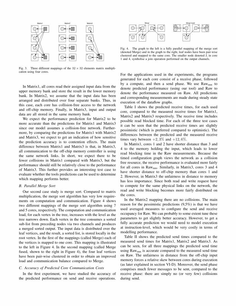
1
3
4
2
1
3
4
2
1
3
4
2
Matrix1 Matrix2 Matrix3
Fig. 3. Three different mappings of the 32× 32 elements matrix multipli-cation using four cores.
In Matrix1, all cores read their assigned input data from theupper memory bank and store the result in the lower memorybank. In Matrix2, we assume that the input data has beenarranged and distributed over four separate banks. Thus, inthis case, each core has collision-free access to the networkand off-chip memory. Finally, in Matrix3, input and outputdata are all stored in the same memory bank.
We expect the performance prediction for Matrix2 to bemore accurate than the predictions for Matrix1 and Matrix3since our model assumes a collision-free network. Further-more, by comparing the predictions for Matrix1 with Matrix2and Matrix3, we expect to get an indication of how sensitivethe prediction accuracy is to contention effects. The maindifference between Matrix1 and Matrix3 is that, in Matrix3,all communication to the off-chip memory controller is usingthe same network links. In short, we expect there to befewer collisions in Matrix1 compared with Matrix3, but theperformance should still be relatively close to the performanceof Matrix3. This further provides an interesting test case toevaluate whether the tools predictions can be used to determinewhich mapping performs better.
B. Parallel Merge Sort
Our second case study is merge sort. Compared to matrixmultiplication, the merge sort algorithm has very low require-ments on computation and communication. Figure 4 showstwo different mappings of the merge sort algorithm using 7and 5 cores, respectively. The computation and communicationload, for each vertex in the tree, increases with the level as thetree narrows down. Each vertex in the tree consumes a sortedsub-list from preceding nodes via two channels and producesa merged sorted output. The input data is distributed over theleaf vertices, and the result, a sorted list, is stored locally in theroot vertex. In the first of the mappings (called Merge) each ofthe vertices is mapped to one core. This mapping is illustratedto the left in Figure 4. In the second mapping (called Mergefused, shown to the right in Figure 4), the four leaf verticeshave been pair-wise clustered in order to obtain an improvedload and communication balance compared to Merge.
C. Accuracy of Predicted Core Communication Costs
In the first experiment, we have studied the accuracy ofthe predicted performance on send and receive operations.
1 2 3 4
6
J J1 2 3 4
65 7
Merge Merge fused
Fig. 4. The graph to the left is a fully parallel mapping of the merge sort(denoted Merge) and in the graph to the right, leaf nodes have been pair-wiseclustered and mapped to the same core. The smaller node denoted J, in core1 and 4, symbolise a join operation performed on the output channels.
For the applications used in the experiments, the programsgenerated for each core consist of a receive phase, followedby a compute, and then a send phase. We use Rawmm todenote predicted performance (using our tool) and Raw todenote the performance measured on Raw. All predictionsand corresponding measurements are made during steady stateexecution of the dataflow graphs.
Table I shows the predicted receive times, for each usedcore, compared to the measured receive times for Matrix1,Matrix2 and Matrix3 respectively. The receive time includespossible read blocked time. For each of the three test casesit can be seen that the predicted receive times are slightlypessimistic (which is preferred compared to optimistic). Thedifferences between the predicted and the measured receivetimes vary between +2, 3% and +12, 6%.
In Matrix1, cores 1 and 2 have shorter distance than 3 and4 to the memory holding the input, which leads to lowerread blocking time in the Raw measurements. Because thetimed configuration graph views the network as a collisionfree resource, the receive performance is evaluated more fairlyfor all cores in Rawmm. Similarly, in Matrix3, cores 3 and 4have shorter distance to off-chip memory than cores 1 and2. However, in Matrix3 the unfairness in distance to memoryhas less importance. Since both read and write request haveto compete for the same physical links on the network, theread and write blocking becomes more fairly distributed onthe cores.
In the Matrix2 mapping there are no collisions. The mainreason for the pessimistic predictions (9,5%) is that we haveused averaged measures to configure the send and receiveoccupancy for Raw. We can probably to some extent tune theseparameters to get slightly better accuracy. However, to get afully accurate prediction we would need to model executionat instruction-level, which would be very costly in terms ofmodelling performance.
Table II shows the predicted send times compared to themeasured send times for Matrix1, Matrix2 and Matrix3. Ascan be seen, for all three mappings the predicted send timeusing Rawmm is accurate compared to the measured send timeon Raw. The unfairness in distance from the off-chip inputmemory forces a relative skew between cores during execution(as later explained in section VI-D). Moreover, the send phasecomprises much fewer messages to be sent, compared to thereceive phase: there are simply no (or very few) collisionsduring send.

TABLE IMATRIX STEADY STATE RECEIVE TIME (CLOCK CYCLES)
Application Core ID Rawmm Raw diff.Matrix1 1 1790 1589 +12,6%
2 1790 1589 +12,6%3 1790 1750 +2,3%4 1790 1750 +2,3%
Matrix2 1 1600 1461 +9,5%2 1600 1461 +9,5%3 1600 1461 +9,5%4 1600 1461 +9,5%
Matrix3 1 1828 1701 +7,5%2 1814 1626 +11,6%3 1800 1716 +4,9%4 1786 1716 +4,1%
TABLE IIMATRIX STEADY STATE SEND TIME (CLOCK CYCLES)
Application Core ID Rawmm Raw diff.Matrix1 1 408 408 0%
2 408 408 0%3 408 408 0%4 408 408 0%
Matrix2 1 408 408 0%2 408 408 0%3 408 408 0%4 408 408 0%
Matrix3 1 408 408 0%2 408 408 0%3 408 408 0%4 408 408 0%
We will now discuss our corresponding experiment on sendand receive times for the merge sort application. In thisexperiment only core-to-core communication is utilised andthe communication consists of very small messages (1 to 4words). Furthermore, we have deliberately designed one of themappings (Merge) to force unbalanced core communicationand computation loads. This experiment is expected to give anindication on how accurately Rawmm models short messagingand unbalanced communication. The predicted send timescompared to the measured ones can be seen in Table III. ForMerge, the predicted times are exact or very accurate. Cores1,2,4, and 7 compute the leaf vertices, which also generate theinput in the parallel merge tree. Thus, no receive operations areissued by these cores. However, for Merge fused, we see thatRawmm has evaluated the receive time 75% higher, comparedto the measurements on Raw for cores 2 and 3. The reasonis that the computation times for cores 2 and 3, after theclustering, are now shorter than for the preceding leaf vertices.Since Rawmm models communication pessimistically – in thesense that we only allow one message at a time on a networklink – communication is tighter synchronised in our model.This can introduce blocking times in communication betweencores with unbalanced workloads, which are not experiencedon Raw.
In Table IV we compare send times for the two differentmappings of the merge sort algorithm. As can be seen in thetable, the predicted send times are fairly close to the measured
TABLE IIIMERGE STEADY STATE RECEIVE TIME (CLOCK CYCLES)
Application Core ID Rawmm Raw diff.Merge 1 0 0 +0%
2 16 16 +0%3 16 16 +0%4 0 0 +0%5 0 0 +0%6 29 28 +3,6%7 0 0 +0%
Merge fused 1 0 1461 +9,5%2 42 24 +75%3 42 24 +75%4 0 0 +0%5 0 0 +0%6 29 28 +3,6%7 0 0 +0%
times (the difference is 9,1% or less).
TABLE IVMERGE STEADY STATE SEND TIME (CLOCK CYCLES)
Application Core ID Rawmm Raw diff.Merge 1 85 79 +7,6%
2 22 22 +0%3 22 22 +0%4 85 79 +7,6%5 85 79 +7,6%6 0 0 +0%7 85 79 +7,6%
Merge fused 1 24 22 +9,1%2 22 22 +0%3 22 22 +0%4 24 22 +9,1%5 0 0 +0%6 0 0 +0%7 0 0 +0%
D. Latency and Throughput Measurements
In the second part of the experiments, we have used thesame mappings to compare predicted and measured end-to-end-latency and throughput. We also evaluate whether thepredictions, despite potential inaccuracy, can be used to rankthe mappings correctly with respect to shortest latency andhighest throughput.
The mappings are self-timed, meaning that synchronisationis handled at run-time [24]. Initially, a self-timed graph exe-cutes a non-steady state and later, after a number of iterations,converges to a steady-state schedule.
Figure 5 illustrates the dynamic behaviour for the self-timed mapping of the Merge application. Cores computing theupstream actors in the dataflow graph with lower workloadfinish faster and can proceed with the next iteration of theschedule, as long as the network buffer is large enough tostore the produced data. As shown in the figure, core 1 hasstarted its fourth iteration when core 6 begins computing itsfirst iteration. When network buffers are full, a steady stateexecution is naturally forced.
Figure 6 shows the predicted latencies (in clock cycles), forMerge and Merge fused, compared to the measured latencies

1
1
1
1
2
3
4
5
6
7
2 3 4 5
2 3 4 5
2 3 4 5
t
Core
20 21 22
20 21 22
20 21 22
Fig. 5. Skewing experienced in the unbalanced Merge algorithm. Thenumbers represent the firing count of each actor, and the distance in timebetween the firings is dependent on the network buffer capacity.
Fig. 6. Comparison of predicted (Rawmm) and measured (Raw) end-to-endlatency for Merge and Merge fused.
as a function of the current iteration. The figure shows atwhich iteration each of the mappings reaches a steady state ofexecution, i.e. when the latency curve levels out. We see that,for Merge, the measured latency is underestimated by a factorof 2. This is explained by the fact that the machine modelis currently not able to model buffer capacity of the on-chipnetwork. Thus, the difference in iteration count between thefirst upstream actor and the last actor in the graph is largeron Raw than in the modelled execution of Raw. To tightenthe latency predictions for graphs with unbalanced communi-cation, we need to account for network buffer capacity in themachine model.
For Merge fused, we see that the latency has rather beenoverestimated, but is closer to the measured latency. Thereason is that both the workload and the communication inMerge fused is better balanced than in Merge (after clusteringcore 1 with 5 and core 3 with 7), which forces Merge fusedto reach a steady state after fewer iterations.
If we rank the predicted latencies of Merge and Mergefused, even if the predictions have varying accuracy, we stillsee that an optimisation decision based on the predictionswould (for this case) correctly identify Merge fused as thebetter mapping.
Figure 7 shows the predicted end-to-end latencies for
Fig. 7. Comparison of the modelling accuracy of the computation latencyof three different mappings of the parallel matrix multiplication.
Matrix1, Matrix2 and Matrix3, compared to the measuredlatencies on Raw. We see that the different mappings ofthe matrix multiplication converge to steady state at differentnumbers of iterations. Unlike in the merge sort experiment, thecomputation tasks distributed on the cores is naturally loadbalanced. The reason that the different implementations ofthe matrix multiplication reach steady state at different pointsin time is that the cores used in the different mappings areaffected by different communication delays due to networkcontention. Contention effects is a large contributing factorcausing an underestimate of the latencies for Matrix1 andMatrix3. This can be verified by observing that the plot forMatrix2 on Rawmm and Raw (which is a contention freemapping), is fairly accurate compared to the predictions forMatrix1 and Matrix3. However, if we rank the predicted steadystate latencies for all mappings, we see that an optimisationdecision based on latency minimisation would in this casecorrectly suggest Matrix3 better than Matrix 1 and Matrix2as the best alternative of the three.
Table V shows the predicted and the measured throughputsfor Merge (with 4,4% difference) and Merge fused (with 10%difference). The predictions are fairly close to the measure-ments on Raw for both Merge and Merge fused. We alsosee that both the predicted and the measured throughputsshow that Merge has a higher throughput than Merge fused.When optimising for throughput, our predictions correctly rankMerge better than Merge fused.
Finally, Table VI shows the corresponding comparisons forMatrix1, Matrix2 and Matrix3. Note that, unlike in all theother experiments, our model has predicted slightly optimisticthroughputs. However, if we rank both the predicted through-puts and the measured throughputs, we see that the predictionswill be ranked in the same order as for the measured ones.Thus, if using the predictions for throughput optimisation, ourtool finds the best cases for this example as well.
VII. CONCLUSION
In this paper we have presented our achievements onbuilding an iterative manycore code mapping tool. In order

TABLE VMERGE STEADY STATE PERIODICITY (CLOCK CYCLES)
Application Rawmm Raw diffMerge 119 104 +4,4%Merge fused 132 120 +10%
TABLE VIMATRIX STEADY STATE PERIODICITY IN (CLOCK CYCLES)
Application Rawmm Raw diffMatrix1 19249 19434 -0,9%Matrix2 19059 19143 -0,4%Matrix3 19248 19401 -0,8%
to provide estimates of performance, we have developed amachine model which abstracts a certain category of manycorearchitectures. We model the applications using synchronousdataflow, and the performance estimates are computed usingan executable intermediate representation called timed config-uration graph.
We have presented an evaluation in terms of the predictionaccuracy of our tool and whether the predictions can be usedto identify a better mapping. It is shown that communicationtimes between cores are predicted slightly pessimistic, stillfairly close to measured performance, with respect to the highlevel of modelling. Our comparisons indicate that, for the smallset of mappings so far explored in the experiments, the toolcan correctly rank different mappings with respect to highestthroughput or shortest latency. However, the comparisons alsoreveal that the predictions of end-to-end latency for graphswith unbalanced communication can be quite inaccurate. Thiswas demonstrated to mainly depend on the high abstractionlevel of on-chip communication implemented by the IR,which currently does not capture the buffer capacity or linkconcurrency of the network.
To increase the accuracy and the reliability of end-to-end latency measurements on dataflow graphs, we plan toinvestigate inclusion of network buffer capacity and modellinglink concurrency in the intermediate representation. We areespecially interested in exploring automatised tuning methods,using feedback information from the abstract interpreter, inorder to direct and improve the mapping of application graphs.
ACKNOWLEDGEMENT
The authors would like to thank Dr. Veronica Gaspes atHalmstad University and the anonymous reviewers whosecomments helped improving this paper. This work has beenfunded by research grants from the Knowledge Foundationunder the CERES contract.
REFERENCES
[1] E. Dahlman, S. Parkvall, J. Skold, and P. Beming, 3G Evolution: HSPAand LTE for Mobile Broadband, 2nd ed. Academic Press, 2008.
[2] M. I. Gordon, W. Thies, and S. Amarasinghe, “Exploiting Coarse-Grained Task, Data, and Pipeline Parallelism in Stream Programs,” inProc. of Twelfth Int’l. Conf. on Architectural Support for ProgrammingLanguages and Operating Systems, 2006, pp. 152–162.
[3] E. A. Lee and D. G. Messerschmitt, “Static Scheduling of SynchronousData Flow Programs for Signal Processing,” IEEE Trans. on Computers,vol. 36, no. 1, pp. 24–35, January 1987.
[4] M. B. Taylor, J. Kim, J. Miller, D. Wentzlaff, F. Ghodrat, B. Greenwald,H. Hoffman, P. Johnson, J.-W. Lee, W. Lee, A. Ma, A. Saraf, M. Seneski,N. Shnidman, V. Strumpen, M. Frank, S. Amarasinghe, and A. Agar-wal, “The Raw Microprocessor: A Computational Fabric for SoftwareCircuits and General-Purpose Programs,” IEEE Micro, vol. 22, no. 2,pp. 25–35, 2002.
[5] H. El-Rewini, H. Ali, and T. Lewis, “Task Scheduling in MultiprocessingSystems,” IEEE Computer, vol. 28, no. 12, pp. 27–37, Dec 1995.
[6] V. Sarkar, Partitioning and Scheduling Parallel Programs for Multipro-cessors. Cambridge, MA, USA: MIT Press, 1989.
[7] V. Kianzad and S. Bhattacharyya, “Efficient Techniques for Clusteringand Scheduling onto Embedded Multiprocessors,” IEEE Trans. onParallel and Distributed Systems, vol. 17, no. 7, pp. 667–680, July 2006.
[8] G. C. Sih, “Multiprocessor Scheduling to Account for InterprocessorCommunication,” Ph.D. dissertation, EECS Department, University ofCalifornia, Berkeley, CA 94720, USA, April 1991.
[9] J. L. Pino and E. A. Lee, “Hierarchical Static Scheduling of DataflowGraphs onto Multiple Processors,” in Proc. of IEEE Int’l Conf. onAcoustics, Speech, and Signal Processing, 1995, pp. 2643–2646.
[10] A. Ghamarian, M. Geilen, S. Stuijk, T. Basten, B. Theelen, M. Mousavi,A. Moonen, and M. Bekooij, “Throughput Analysis of SynchronousData Flow Graphs,” Proc. of Int’l Conf. on Application of Concurrencyto System Design, pp. 25–36, 2006.
[11] S. Stuijk, T. Basten, M. C. W. Geilen, and H. Corporaal, “MultiprocessorResource Allocation for Throughput-Constrained Synchronous DataflowGraphs,” in Proc. of the 44th annual conf. on Design automation. NewYork, NY, USA: ACM, 2007, pp. 777–782.
[12] N. Bambha, “Intermediate Representations for Design Automation ofMultiprocessor DSP Systems,” in Design Automation for EmbeddedSystems. Kluwer Academic Publishers, 2002, pp. 307–323.
[13] S. S. Battacharyya, “Optimization Trade-offs in the Synthesis of Soft-ware for Embedded DSP,” in Workshop on Compiler and ArchitectureSupport for Embedded Systems, Washington, D.C, 1999.
[14] C. Brooks, E. A. Lee, X. Liu, S. Neuendorffer, Y. Zhao, and H. Zheng,“Heterogeneous Concurrent Modeling and Design in Java (Volume 1:Introduction to Ptolemy II),” EECS Dept., University of California,Berkeley, Tech. Rep. UCB/EECS-2008-28, Apr 2008.
[15] D. Culler, R. Karp, and D. Patterson, “LogP: Towards a Realistic Modelof Parallel Computation,” in in Proc. of ACM SIGPLAN Symp. onPrinciples and Practices of Parallel programming, May 1993, pp. 1–12.
[16] A. Alexandrov, M. F. Ionescu, K. E. Schauser, and C. J. Scheiman,“LogGP: Incorporating Long Messages into the LogP Model - OneStep Closer Towards a Realistic Model for Parallel Computation.” inProc. of the seventh annual ACM Symp. on Parallel Algorithms andArchitectures, 1995, pp. 95–105.
[17] C. A. Moritz and M. I. Frank, “LoGPC: Modeling Network Contentionin Message-Passing Programs,” IEEE Trans. on Parallel and DistributedSystems, vol. 12, no. 4, pp. 404–415, 2001.
[18] C. A. Moritz, D. Yeung, and A. Agarwal, “SimpleFit: A Frameworkfor Analyzing Design Tradeoffs in Raw Architectures,” IEEE Trans. onParallel and Distributed Systems, vol. 12, no. 6, pp. 730–742, June 2001.
[19] M. B. Taylor, W. Lee, S. P. Amarasinghe, and A. Agarwal, “ScalarOperand Networks,” IEEE Trans. on Parallel and Distributed Systems,vol. 16, no. 2, pp. 145–162, 2005.
[20] J. Bengtsson, “A Set of Models for Manycore Performance EvaluationThrough Abstract Interpretation of Timed Configuration Graphs,” Schoolof IDE, Tech. Rep. IDE0856, 2008.
[21] T. M. Parks, “Bounded Scheduling of Process Networks,” Ph.D. disser-tation, EECS Department, University of California, Berkeley, CA 94720,USA, 1995.
[22] G. Kahn, “The Semantics of a Simple Language for Parallel Program-ming,” in Proc. of IFIP Congress 74, J. L. Rosenfeld, Ed. Stockholm,Sweden: North-Holland Publishing Company, August 5-10 1974, pp.471–475.
[23] M. B. Taylor, “The Raw Processor Specification,” CSAIL, MIT, Cam-bridge, MA, Tech. Rep., 2003.
[24] E. Lee and S. Ha, “Scheduling Strategies for Multiprocessor Real-timeDSP,” in Proc. of IEEE Glob’l. Telecomm. Conf., 1989, and Exhibition.Communications Technology for the 1990s and Beyond., Nov 1989, pp.1279–1283 vol.2.