Modelling Uncertainties in Offshore

Turbine Availability

TIM BEDFORD, ATHENA ZITROU, LESLEY WALLS and KEVIN WILSON

Department of Management Science

University of Strathclyde, Glasgow, Scotland

tim.bedford@strath.ac.uk

KEITH BELL, DAVID INFIELD

Dept of EEE

UK EPSRC PROJECT No EP/I017380/1

Overview

• General Context

• Measures of performance

• Types of uncertainty

• Availability growth problem

• Decision support example

• Estimation of uncertainty

• Summary

Offshore Wind Farm Context

• Key contributor to UK

renewables target

– 30% generation capacity by 2020

• Technical availability key

performance indicator

– UK round 1 OWF average annual

availability 80.2%

Source: Feng et al(2011)

– Target annual OWF availability of

97%-98% for financial viability

• Wind uncertainty compounded in

output uncertainty

Windfarm in North Hoyle (off North Wales)

Windfarm Availability

Offshore challenges • Harsh environmental conditions

• Limited access

• Expensive maintenance actions

• Relatively new systems

• Large fleets

Assess technological performance

• Reliability, operations and maintainability

drive availability

Availability Modelling Goal

• Develop a mathematical model to: 1. assess offshore wind farm availability growth during

early operational life (up to 5 years of operation)

2. model state-of-knowledge uncertainty

• Purpose of availability growth model is to: 1. provide insight into interventions to achieve

availability growth

2. understand scale of uncertainty and hence manage

• Model to be a “tool kit” – generic and specific

applications

Model Boundaries

• Offshore wind farm comprises:

– Wind turbines - subsystems

– Subsea cables

– Offshore transformer

Two owners – Generator, OFTO Risk sharing/contract

Point value models for O&M

• TU Delft

– Assesses long-term farm availability and O&M costs

– Uses Monte Carlo simulation

– Simulates maintenance hourly operations over a twenty year

period.

– Uses extensive weather simulation and average failure rates

• ECN Wind Energy

– Assesses overall O&M cost

– Spreadsheet-based method

– Average failure rates, availability of maintenance resources,

access on site

– Linked to @Risk to perform uncertainty analysis

• Strathclyde (EEE)

– Empirical ROCOF used for MC simulation

• Early life failures

• Cost of insurance/cost of finance

• Lack of performance data

• Weather/sea states/environment

• Logistics market underdeveloped

• Shifting government interest

8

Major problems - uncertainties

Definition of Availability

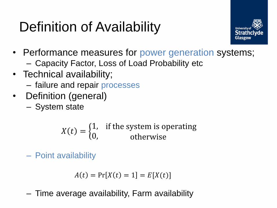
• Performance measures for power generation systems; – Capacity Factor, Loss of Load Probability etc

• Technical availability; – failure and repair processes

• Definition (general) – System state

𝑋 𝑡 = 1,0, if the system is operating

otherwise

– Point availability

𝐴 𝑡 = Pr 𝑋 𝑡 = 1 = 𝐸[𝑋(𝑡)]

– Time average availability, Farm availability

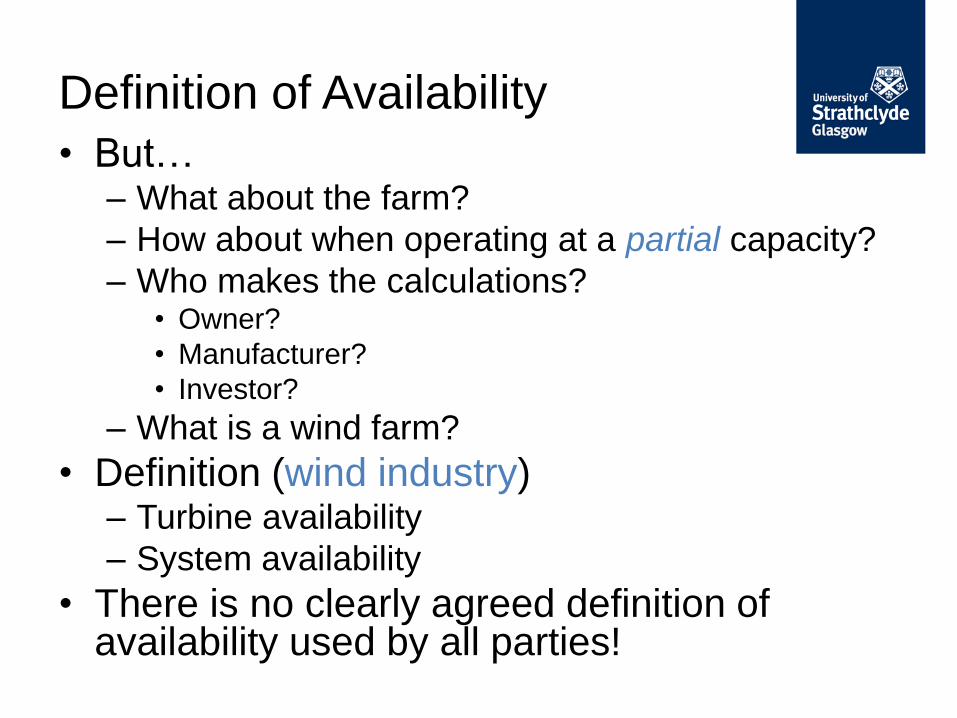
Definition of Availability

• But… – What about the farm?

– How about when operating at a partial capacity?

– Who makes the calculations? • Owner?

• Manufacturer?

• Investor?

– What is a wind farm?

• Definition (wind industry) – Turbine availability

– System availability

• There is no clearly agreed definition of availability used by all parties!

Maximum output

Multiple system states

Availability-informed capability

Installed output

• Due to the costs of repair and production loss and logistic delays an offshore wind farm will operate in degraded states.

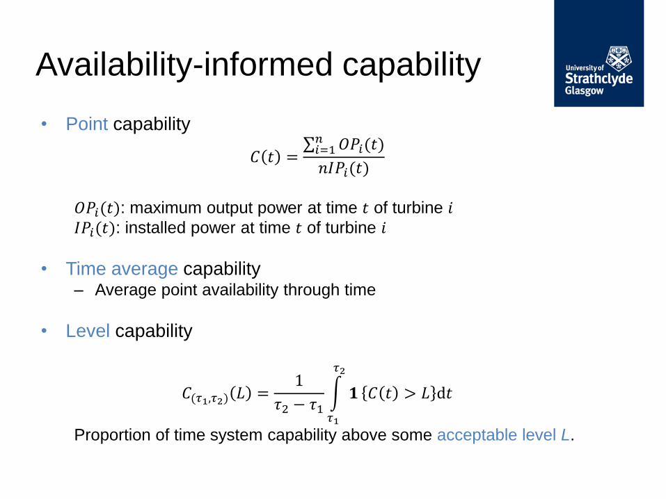
Availability-informed capability

• Point capability

𝐶 𝑡 = 𝑂𝑃𝑖(𝑡)𝑛𝑖=1

𝑛𝐼𝑃𝑖(𝑡)

𝑂𝑃𝑖(𝑡): maximum output power at time 𝑡 of turbine 𝑖 𝐼𝑃𝑖(𝑡): installed power at time 𝑡 of turbine 𝑖

• Time average capability – Average point availability through time

• Level capability

𝐶(𝜏1,𝜏2) 𝐿 =1

𝜏2 − 𝜏1 𝟏

𝜏2

𝜏1

𝐶 𝑡 > 𝐿 d𝑡

Proportion of time system capability above some acceptable level L.

Estimate capability

Long -term (from time t= 0)

Short-term (from time 𝑠 > 0)

Metric to judge overall capability

Metric to judge short term variability and controlability through maintenance strategy

Uncertainty & Assessments

Role of uncertainty • Need to represent in availability models and explore

implications in reliability/availability assessments

Aleatory uncertainty • Natural variability in the system

• Failure times, repair times….

• Irreducible

Epistemic/state of knowledge uncertainty • Lack of knowledge of the system and environment

• Limitations in assessing parameters of key elements

• Reducible by better information

• Nuclear power plants (NPPs)

• WASH 1400 report gave the probability of a

frequency…of core melt

• Difficult to understand what this means –

imagine a notional large population of NPPs of

same design and ask about number of core

melts in 1000 years…

15

Policy interest in epistemic

uncertainty

• …is another persons aleatory uncertainty

• Farm level variability arising from

epistemic uncertainties are of interest to

financiers/insurers

16

One persons epistemic uncertainty…

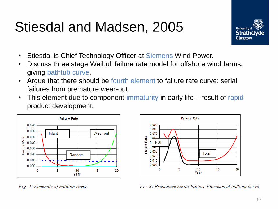
Stiesdal and Madsen, 2005

17

• Stiesdal is Chief Technology Officer at Siemens Wind Power.

• Discuss three stage Weibull failure rate model for offshore wind farms,

giving bathtub curve.

• Argue that there should be fourth element to failure rate curve; serial

failures from premature wear-out.

• This element due to component immaturity in early life – result of rapid

product development.

18

• Medium to long term behaviour should be similar to existing (smaller scale) systems – modulo some uncertainty (on long term)

• Short term behaviour can be (much) worse due to design, manufacturing and operating errors

• Availability growth happens by recognizing and eliminating these errors

19

Conceptual approach

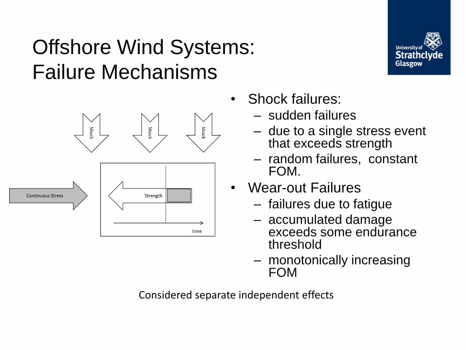
Offshore Wind Systems:

Failure Mechanisms

• Shock failures: – sudden failures

– due to a single stress event that exceeds strength

– random failures, constant FOM.

• Wear-out Failures – failures due to fatigue

– accumulated damage exceeds some endurance threshold

– monotonically increasing FOM

Considered separate independent effects

Target vs. Actual Reliability:

Failure Mechanisms

𝑥

Early life

𝑥

Early life Maturity

PATTERN A

PATTERN B

× 𝑠

PATTERN B

PATTERN A

Shock Failures Wear-out

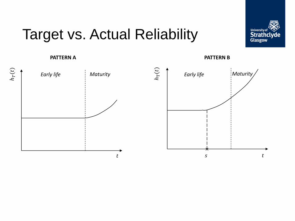
Target vs. Actual Reliability

𝑡

Early life Maturity

PATTERN A

𝑡

Early life Maturity

PATTERN B

× 𝑠

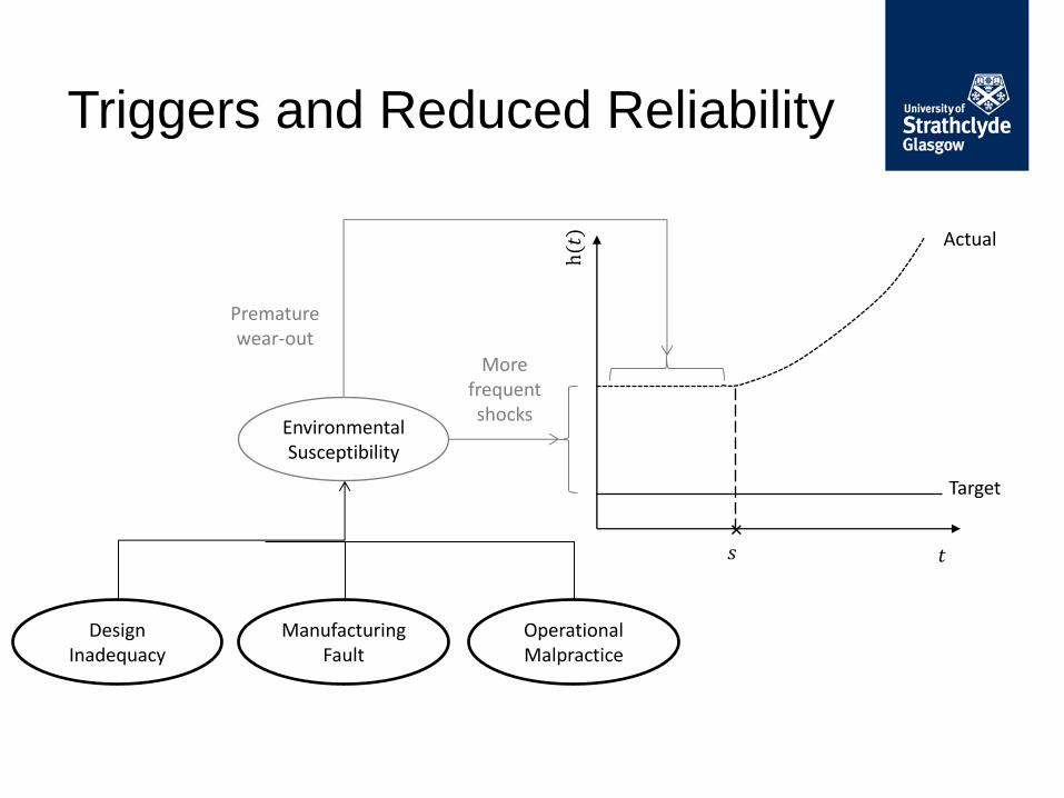
Triggers and Reduced Reliability

𝑡

Target

Actual

𝑠 ×

Design Inadequacy

Manufacturing Fault

Operational Malpractice

Environmental Susceptibility

Premature wear-out

More frequent shocks

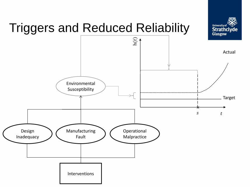
Triggers and Reduced Reliability

𝑡

Target

Actual

𝑠 ×

Design Inadequacy

Manufacturing Fault

Operational Malpractice

Environmental Susceptibility

Interventions

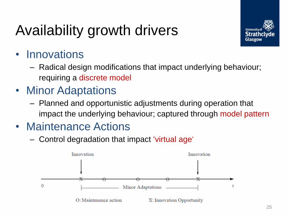
• Innovations – Radical design modifications that impact underlying behaviour;

requiring a discrete model

• Minor Adaptations – Planned and opportunistic adjustments during operation that

impact the underlying behaviour; captured through model pattern

• Maintenance Actions – Control degradation that impact ‘virtual age’

25

Availability growth drivers

Major Innovation Design

Minor Adjustments

Availability

Uptime Downtime

Target FOM

Actual FOM

Major Innovation Vessel Strategy

Actual Restoration

Major Innovation Spares Policy

Design Inadequacy

Operational Malpractice

Manufacturing Fault

Logistics Time (spares)

Waiting Time Travelling Time

Target Restoration

Waiting Time

Minor Adjustments

Shocks Wear-out

Environmental Susceptibility

Manufacturing Fault at

Subassembly 1

Manufacturing Fault at

Subassembly n

Error in Quality Process

Crew Error

𝑡 − 1

Subassembly 1 Fails

Subassembly n Fails

Operational Malpractice at Subassembly 1

Operational Malpractice at Subassembly n

𝑡

Subassembly 1 Fails

Subassembly n Fails

Operational Malpractice at Subassembly 1\

Operational Malpractice at Subassembly n

Crew Error

Farm Availability

Failure Restoration

Virtual Age Repair

experience

History Maintenance

Actions

Downtime

Repair Time

Waiting Time Travel Time Logistics Time

(Spares)

Availability-informed Capability

Subassemblies’ State

Interventions

Failure

Waiting Time Travel Time Logistics Time

(Spares)

Repair Time

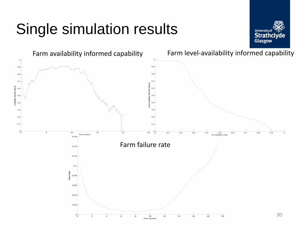
Uncertainty

• We simulate an offshore wind farm with 200 turbines,

each of which has 18 sub-assemblies.

• We assume minor adaptions are made on each sub-

assembly continuously.

• Innovations are made on each sub-assembly a single

time in the summer for each of the first 4 years of the life

of the farm.

• The simulation is run for the first 20 years of operation of

the wind farm.

29

Illustrative example

0 2 4 6 8 10 12 14 16 18 200

0.02

0.04

0.06

0.08

0.1

0.12

0.14

0.16

Time (years)

Failu

re R

ate

0 5 10 15 20 250

0.1

0.2

0.3

0.4

0.5

0.6

0.7

0.8

0.9

1

Time (years)

Ava

ilabi

lity

info

rmed

cap

acity

30

Single simulation results

Farm availability informed capability Farm level-availability informed capability

Farm failure rate

0 0.1 0.2 0.3 0.4 0.5 0.6 0.7 0.8 0.9 10

0.1

0.2

0.3

0.4

0.5

0.6

0.7

0.8

0.9

1

Acceptable Level

Leve

l Ava

ilabi

lity

Info

rmed

Cap

acity

31

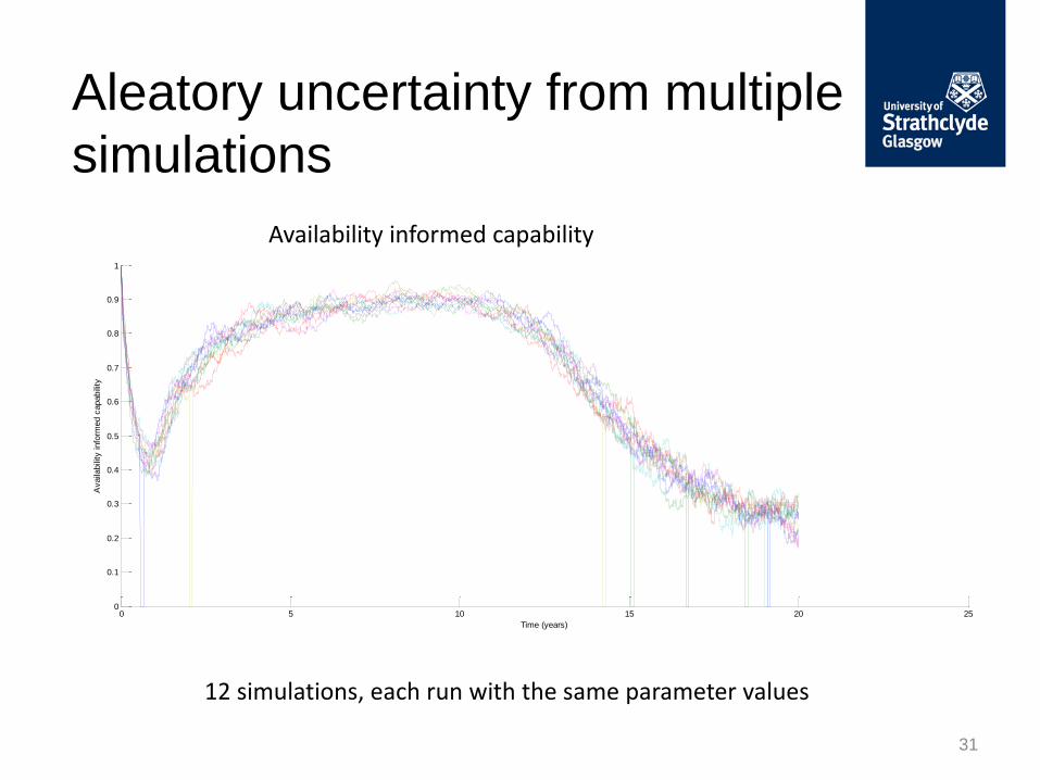
Aleatory uncertainty from multiple

simulations

0 5 10 15 20 250

0.1

0.2

0.3

0.4

0.5

0.6

0.7

0.8

0.9

1

Time (years)

Availa

bili

ty info

rmed c

apabili

ty

12 simulations, each run with the same parameter values

Availability informed capability

32

Epistemic uncertainty from multiple

parameter values

0 5 10 15 20 250

0.1

0.2

0.3

0.4

0.5

0.6

0.7

0.8

0.9

1

Time (years)

Availa

bili

ty info

rmed c

apabili

ty

Setting a0=0.05,0.075,0.1 (r,g,b) in failure intensities.

0 5 10 15 20 250

0.1

0.2

0.3

0.4

0.5

0.6

0.7

0.8

0.9

1

Time (years)

Availa

bili

ty info

rmaed c

apabili

ty

Setting b0=0.7,0.8,0.9 (g,b,r) in failure intensities.

0 5 10 15 20 250

0.1

0.2

0.3

0.4

0.5

0.6

0.7

0.8

0.9

1

Time (years)

Availability info

rmed c

apacity

Setting a0=5,6,7 (g,b,r) in restoration intensities.

0 5 10 15 20 250

0.1

0.2

0.3

0.4

0.5

0.6

0.7

0.8

0.9

1

Time (years)

Availability info

rmed c

apability

Setting b0=3,4,5 (g,b,r) in restoration intensities.

• Running the simulation multiple times gives an

estimate of the aleatory uncertainty.

• Running the simulation on multiple parameter

values gives an estimate of the epistemic

uncertainty.

• How do we choose the range of parameter

values to run the simulation at?

33

Estimation of Uncertainty

• Different viewpoints of OEM, generator, OFTO, maintenance provider, financial markets etc

• Cost/benefit cases for testing and instrumentation

• Need to create robust system that manages risks through life – so control perspective rather than static risk view

34

Whose uncertainty?

• 2 stage Bayesian model – each baseline failure rate drawn from common Gamma

• Expert Judgement – absolute

• Expert Judgement – relative

• Tolerance uncertainty – recognizes impact of environment on similar systems

• Bayesian networks/proportional hazard etc

• REMM approach using FMEA identifying concerns at design stage

35

Bayesian/subjective approaches to

“similar but not identical data”

• Onset of aging…uncertainty

36

Parameterizing appropriately

Onset of aging uncertainty Testing period

37

Heavy Lift Project

• Availability growth is an important concept.

• Capability definition allows for partial performance

states, without compounding impact of wind.

• Getting a handle on the different uncertainties

affecting early life availability of an offshore wind

farm is crucial to decision making.

• Potentially big difference between “steady state”

system behaviour and early life behaviour

• Model allows us to test impact of uncertainties at

subsystem level on the overall performance. 38

Summary

39