IOP PUBLISHING PHYSICS IN MEDICINE AND BIOLOGY

Phys. Med. Biol. 58 (2013) R63–R96 doi:10.1088/0031-9155/58/12/R63

TOPICAL REVIEW

Modelling the physics in the iterative reconstructionfor transmission computed tomography

Johan Nuyts1, Bruno De Man2, Jeffrey A Fessler3, Wojciech Zbijewski4

and Freek J Beekman5

1 Department of Nuclear Medicine and Medical Imaging Research Center, KU Leuven, Leuven,Belgium2 GE Global Research, Niskayuna, New York, USA3 Electrical Engineering and Computer Science Department, University of Michigan, Ann Arbor,MI, USA4 Department of Biomedical Engineering, Johns Hopkins University, Baltimore,MD 21205-2109, USA5 Radiation Detection and Medical Imaging, Delft University of Technology, Delft,The Netherlands

E-mail: johan.nuyts@uz.kuleuven.be

Received 11 April 2012, in final form 4 April 2013Published 5 June 2013Online at stacks.iop.org/PMB/58/R63

AbstractThere is an increasing interest in iterative reconstruction (IR) as a key toolto improve quality and increase applicability of x-ray CT imaging. IR hasthe ability to significantly reduce patient dose; it provides the flexibility toreconstruct images from arbitrary x-ray system geometries and allows one toinclude detailed models of photon transport and detection physics to accuratelycorrect for a wide variety of image degrading effects. This paper reviewsdiscretization issues and modelling of finite spatial resolution, Compton scatterin the scanned object, data noise and the energy spectrum. The widespreadimplementation of IR with a highly accurate model-based correction, however,still requires significant effort. In addition, new hardware will provide newopportunities and challenges to improve CT with new modelling.

S Online supplementary data available from stacks.iop.org/PMB/58/R63/mmedia

1. Introduction

Computed tomography (CT) was introduced as a clinical imaging tool in the 1970s. Since then,it has seen impressive improvements in hardware and software. Over the last few decades,the number of detector rows has increased continuously, effectively turning multi-detectorrow CT systems into cone-beam CTs (CBCTs). To increase the scanning speed, the rotationtime has been reduced, reaching values below 300 ms per rotation, and the original approachof sequential circular scanning has been replaced by helical (spiral) orbits (Kalender 2006).In the last 20 years, flat-panel detectors have been introduced for planar and tomographic

0031-9155/13/120063+34$33.00 © 2013 Institute of Physics and Engineering in Medicine Printed in the UK & the USA R63

R64 Topical Review

x-ray imaging (Kalender and Kyriakou 2007). These detectors are being used in dedicated CTapplications, such as flexible C-arm CT systems for angiography and cardiac imaging, digitaltomosynthesis for mammography and high-resolution dental imaging. This evolution of thehardware was parallelled by new developments in image reconstruction software. New ‘exact’analytical reconstruction algorithms have been derived for CT with 2D detectors, movingalong helical (Katsevich 2002, Noo 2003) and other more exotic acquisition trajectories (Packet al 2004). In addition, as a side effect of these developments, new insight has been gained inthe reconstruction from truncated projection (Clackdoyle and Defrise 2010).

Although analytical reconstruction algorithms usually produce excellent images, thereis a growing interest in the iterative reconstruction (IR). One important reason for this is agrowing concern about the radiation doses delivered to the patients. Another reason is thehigher flexibility and robustness of iterative algorithms, which will allow new CT designs thatwould pose problems for analytical reconstruction algorithms.

In IR, one models the fact that there are a finite number of measured rays, whereasanalytical methods are derived assuming a continuum of rays. In contrast to analyticalreconstruction, iterative methods assume right from the start that the image to be reconstructedconsists of a finite number of samples too. This is obviously an approximation, but it allowsapplication of numerical methods to solve the reconstruction problem. The algorithms canbe considered as a feedback mechanism, with a simulator of the CT-physics (re-projection)in the feedback loop. The feed forward loop updates the reconstruction image, based ondeviations between the measured and simulated scans (this usually involves a backprojection).The output of the algorithms is very sensitive to the CT simulator in the feedback loop; foraccurate results, it is essential to use a sufficiently accurate simulator. There is more freedomin the feed forward loop, which can be exploited by algorithm designers to improve the (localor global) convergence properties (De Man and Fessler 2010).

This paper discusses the physics models that are used in the feedback loop. The basicmodel that is often used can be written as follows:

Yi = bi e!!

j li jµ j + si + ni, (1)

where Yi is the measured transmission sinogram value along the projection line i, bi is thecorresponding value that would be measured in the absence of attenuation (blank or aircalibration scan), µ j is the linear attenuation coefficient at voxel j, li j represents the effectiveintersection length of the projection line i with voxel j and si represents possible additivecontributions, such as Compton scatter. The model is completed by assuming a probabilitydistribution for the noise ni. The index i combines all dimensions of the sinogram (includingaxial and transaxial detector positions, view angle); the index j typically represents the threedimensions of the reconstruction volume. An alternative representation is

yi = ln"

bi

Yi ! si

#=

$

j

li jµ j + n"i, (2)

which takes the log-converted data as the input. A noise model for n"i can be obtained by

propagating the noise model for (1) through the logarithm. Many analytical algorithms andsome iterative ones, such as the well-known simultaneous algebraic reconstruction (SART)algorithm (Andersen and Kak 1984, Byrne 2008), use the same weight for all data during thecomputations. This corresponds to assuming that n"

i is independent of i.The models (1) and (2) have several limitations. They assume a monochromatic

transmission source, prior knowledge of the scatter contribution and no detector crosstalk.They cannot accurately account for the finite sizes of the transmission source and the detectorelements and cannot model blurring effects due to a continuous gantry rotation. Although

Topical Review R65

these approximations are acceptable in many applications, there are also many cases wherebetter models have significantly improved the final reconstruction.

Below, we discuss various aspects of the physics model in the iterative CT reconstruction.Section 2 discusses problems and opportunities of the discretization and section 3 showshow the models can be extended to take into account effects limiting the spatial resolution.Compton scatter in the scanned object is discussed in section 4. Section 5 analyses the complexnoise characteristics of data from the energy-integrating x-ray detectors and presents ways toapproximate it. Section 6 briefly discusses the incorporation of the energy spectrum andsection 7 shows how artefacts due to motion can be reduced or eliminated.

2. Discretization

Any practical IR algorithm needs to make accurate approximations of the true, continuousnature of the object. Typically, the reconstructed object is represented as a weighted sum ofa finite set of spatial basis functions, with a grid of cubic, uniform, non-overlapping voxelscovering the reconstructed field of view (FOV) being perhaps the most common and intuitiveexample of such a basis set. The reconstruction algorithm solves for the coefficients of thisexpansion, i.e., the attenuation (or density in polyenergetic reconstruction) of each uniformvoxel in the grid. An alternative, but closely related expansion replaces the voxels with aset of spherically symmetric Kaiser–Bessel functions, known as ‘blobs’ (Lewitt 1990, Matejand Lewitt 1996, Ziegler et al 2006, Carvalho and Herman 2007). During the reconstruction,projections of the object are simulated either by tracing rays and computing intersectionlengths with each basis function (for voxels, common choices are the ray-tracing algorithmsof Siddon (1985) or Joseph (1982)), or by a ‘footprint’-based approach (De Man and Basu2004, Ziegler et al 2006, Long et al 2010). Note that the system model assumed in IR(involving discretized object and detectors) is fundamentally different from the one usedin the derivation of analytical algorithms (where the object is assumed continuous). Thisindicates that notions such as sufficient sampling (e.g., in the case of sparse acquisitions)may not directly translate from the analysis of analytical reconstruction to IR, as discussed inBian et al (2013).

A host of new considerations for object discretization is likely to arise with the growinginterest in the application of IR to time-resolved CT imaging, such as in motion-compensatedcardiac reconstruction (Isola et al 2010, Isola et al 2008) or perfusion imaging on slowlyrotating cone-beam systems (Neukirchen et al 2010). In motion-compensated reconstruction,a new strategy for the computation of basis footprints to account for changes in sampling dueto the motion field was shown to be necessary and developed for the blob-based representation(Isola et al 2008). Examples from cardiac emission tomography suggest that other objectrepresentations such as deformable meshes (Brankov et al 2004, 2005) could provide aninteresting alternative to conventional discretization with voxels or blobs for modelling motionin IR. In perfusion imaging and other applications involving tracking contrast enhancement,IR is enabled by representing the time-varying attenuation (or density) at each location inthe object as a superposition of a finite number of temporal basis functions (e.g., gamma-variate distributions) and then solving for the coefficients of this expansion (Neukirchen et al2010, Johnston et al 2012). This essentially means that the reconstruction problem is nowdecomposed into a set of spatiotemporal basis functions, instead of the purely spatial basisfunctions discussed above. More details on the dynamic aspects of IR are given in section 7.

Here, we discuss some considerations regarding object discretization in IR that ariseregardless of the chosen method of re-projection. In particular, we will review the following:(i) artefacts due to inconsistencies caused by the discrete approximation of true continuous

R66 Topical Review

(A) (B) (C)

Figure 1. (A) FBP reconstruction from simulated projections of a digital abdomen phantom.Simulations were performed on a very fine (4096#4096) grid with 0.125 mm voxels and 16 raystraced per 2 mm detector bin. All reconstructions are presented on a 512#512 grid of 1 mm voxels(‘natural’ voxel size for this geometry with the magnification of 2). The iterative unregularizedordered subset convex (OSC) reconstruction on the 512#512 grid is shown in (B) at a noiselevel matching the FBP image (accomplished by low-pass filtering). Despite better resolution(FWHM of the line pattern), the OSC image is plagued by edge and aliasing artefacts caused byobject discretization. Artefacts are indicated by arrows; in each case, an image of a section of thephantom is also shown using a compressed greyscale to better visualize the artefacts. The OSCreconstruction on a fine grid (1024#1024) followed by downsampling to the same grid as used forFBP is illustrated in (C). The greyscale range is 0.9–1.1 g cm!3 for full images and 1.0–1.02 g cm!3

for image details. Figure taken from Zbijewski and Beekman (2004a). Copyright IOP Publishing2004.

physical objects, (ii) region-of-attention strategies to reduce the computational burden of usingfinely spaced basis functions and (iii) issues related to the use of discrete object and detectormodels in simulation studies of algorithm performance.

2.1. Discretization artefacts in IR

The very fact that the object is discretized into a finite number of basis functions inherentlyleads to discrepancies between the measured projection data and the simulated re-projectionsestimated during the reconstruction (Zbijewski and Beekman 2004a, Pan et al 2009, Hermanand Davidi 2008). The finite-dimensional object representation is thus both a crucial enablerand a potential source of significant errors in reconstruction, as discussed in the generalcontext of (linear) statistical inverse problems in Kaipio and Somersalo (2007). As presentedin Zbijewski and Beekman (2004a) for cubic voxels, even in the case of ‘ideal’ discretizationwhere each voxel represents the average attenuation (or density) of the continuous objectwithin its volume, the simulated re-projection of such a representation will be mismatchedwith the measured projections in areas corresponding to interfaces between tissues. BecauseIR algorithms seek to maximize the agreement between the re-projections and the measureddata, these unintended mismatches may cause artefacts. Typically, such artefacts are mostpronounced around sharp material boundaries and appear as edge overshoots and aliasingpatterns. Figure 1 illustrates these effects for a simulation of a clinical fan-beam CTscanner. No artefacts attributable to object discretization are present in the analytical (filteredbackprojection or FBP) reconstruction onto a grid of ‘natural’ voxels, given by de-magnifieddetector pixel size (figure 1(A)). Figure 1(B) shows the result of IR onto the same object grid,exhibiting the edge and aliasing artefacts explained above.

Intuitively, using many basis functions to represent the object (e.g., smaller voxels) shouldalleviate such discretization-induced artefacts, as has been shown by Zbijewski and Beekman(2004a). In particular, it was demonstrated that while the statistical reconstruction onto avoxel grid typical for analytical reconstruction results in severe edge artefacts (figure 1), the

Topical Review R67

reconstruction on twice as fine a grid followed by binning back onto the ‘natural voxels’ issufficient to remove most of the artefacts (figure 1(C)). The binning step mitigates the increasednoise in the finely sampled reconstruction; this approach has been shown to outperform simplepost-smoothing of the low-resolution reconstructions in terms of the tradeoff between artefactreduction and resolution (Zbijewski and Beekman 2004a). The reconstruction using a finelysampled voxel basis has also been demonstrated to outperform an approach based on smoothingthe measured projections (Zbijewski and Beekman 2006a), which intends to compensate forthe blur introduced by discretization and improve the match between measured and simulatedprojections (Kunze et al 2005). Finally, even though basis functions such as the blobs areexpected to show slightly less-pronounced edge artefacts than square voxels (Matej and Lewitt1996), such artefacts have still been observed in blob-based CT reconstructions (Ziegler et al2006). It has also been shown that, at least in some cases, the voxel-based reconstruction on afine grid outperforms the blob-based reconstruction on a coarser grid in terms of edge artefactreduction (Zbijewski and Beekman 2006a). Some projection operators were demonstratedto be more immune to such artefacts than others (e.g., the trapezoidal separable footprintoutperformed a distance-driven projector in Long et al (2010) in this respect), but in general,the root cause of the problem is using a finite number of basis functions to represent acontinuous object (Pan et al 2009), regardless of the particular form of the basis functionsor projection operator. IR is thus likely to typically require finer object discretizations thananalytical reconstruction to minimize edge artefacts. Note that using more basis functionsmay degrade the conditioning of the reconstruction problem, so that a judicious choice ofregularization may become increasingly important in constraining the solution. Furthermore,the edge and aliasing artefacts due to discretization may occur alongside similar artefactscaused by the Gibbs phenomenon, where the reconstruction algorithm attempts to recoverhigh frequencies lost in the detection process, compound by mismatches between the trueblurring in the system and its model used by the reconstructor, as described in Snyder et al(1987) for emission tomography.

2.2. Non-uniform discretization and other region-of-interest (ROI) techniques

Using fine discretizations to reduce edge artefacts (or for any other purpose) may pose practicalproblems because the reconstruction time increases with the size of the basis set used torepresent the object (the number of elements in the reconstruction grid). This increase couldbe partly mitigated if computations on a fine reconstruction grid could be restricted only tothose areas of the object where the improved discretization is most likely to be beneficial(ROI). One example where this approach could be applied is in the reduction of nonlinearpartial volume effect (NLPV, also known as edge-gradient effect (De Man 2001)), in particulararound metallic implants. NLPV is caused by inconsistencies in projection data arising fromattenuation gradients occurring within the FOV of a single detector cell due to the logarithmicrelationship between attenuation and measured intensity (Glover and Pelc 1980, Joseph andSpital 1981). NLPV is therefore an unavoidable result of using finite detector apertures, butcan be alleviated if the reconstruction accounts for the process of formation of this artefact byfinely discretizing the object space (to better capture the image gradients) and by subsamplingthe detector cells (to capture the averaging of detected intensities across image gradients)(Stayman et al 2013, Van Slambrouck and Nuyts 2012). Since the NLPV artefacts are mostpronounced around high-intensity image gradients, e.g., around metallic implants, strategieswhere the object discretization is made finer only in the vicinity of such structures wereproposed (Stayman et al 2013, Van Slambrouck and Nuyts 2012). In Van Slambrouck andNuyts (2012), the grouped coordinate ascent is employed to allow for a sequential update

R68 Topical Review

(and associated faster convergence) of image regions with different discretization. In Staymanet al (2013), a non-uniform reconstruction grid is applied within an algorithm where priorknowledge of the shape and composition of the implant (e.g., a CAD model) is used to recastthe reconstruction objective function as the estimation of the underlying anatomy and theregistration of the known implant. The discretization of the known implant model is noweasily decoupled from the discretization on the underlying volume, allowing for significantupsampling of only the implant without incurring large computational cost.

The examples discussed above considered spatial basis functions that are most commonlyused in IR of x-ray CT data, i.e., cubic voxels and blobs. Non-uniform discretization couldperhaps be achieved more naturally when using a polygonal mesh to represent the object(similar to a finite-element analysis), as shown for emission tomography in Brankov et al(2004). The mesh is defined by its vertices, whose density is varied throughout the space basedon the level of local image detail. This focuses the computations on the regions of highestdetail, while also benefitting from a likely more compact object representation than in thecase of voxel basis. It remains to be seen whether this approach could benefit IR in x-ray CT,where the image resolution and spatial detail in the reconstructed distributions are significantlyhigher than in emission tomography and the spectrum of detection and estimation tasks differsfrom those in emission tomography.

Another application benefitting from selective use of fine object discretization is high-resolution imaging of large body sites, such as the heart. In this case, the high-resolutionrepresentation of only a selected ROI (e.g., the heart itself) is likely sufficient for diagnosis.Restricting the finely sampled IR only to this ROI would reduce computation, but cannot beachieved with standard IR algorithms because re-projections of the complete FOV are neededto compute the objective function. In Ziegler et al (2008), this limitation is overcome byusing an initial analytical high-resolution reconstruction of the complete volume (relativelycomputationally inexpensive) to compute projections of the volume without the ROI (maskedout from the analytical reconstruction), which are then subtracted from the original data to yieldprojections of the ROI only, which are subsequently reconstructed with IR at high resolution.Related approaches using IR with two different voxel grids were proposed by Hamelin et al(2007, 2010).

A situation where the complete object fills only a relatively small volume within the FOVcould also benefit from an approach that exploits ROI discretization. If the area of the FOVthat does not contribute to the projections (i.e., air surrounding the object) can be identifiedinside the discretized volume through image processing techniques, the forward projectionand backprojection could be limited only to those spatial basis functions that cover the object(attenuator), saving memory and computation time, especially if the forward projector andbackprojector utilize pre-computed voxel footprints (Benson and Gregor 2006).

2.3. Discretization in simulation studies

Development of reconstruction algorithms usually heavily relies on simulation studies, whereprojections of digital phantoms are computed and then reconstructed. Such simulation studiesfrequently rely on discrete representations of the object and the detector, mainly because ofthe flexibility of this approach in capturing the complexities of real anatomy compared tothe alternative approach of analytical modelling. The assessment of reconstruction algorithmsbased on the results of such numerical simulations can however be biased due to the choice ofthe basis set used in the discretization.

In Goertzen et al (2002), several phantoms were simulated using the Siddon ray-tracingalgorithm (Siddon 1985) and voxel image representation for a range of numbers of rays per

Topical Review R69

projection pixel and voxel sizes. FBP reconstructions of these simulations were performed ontoa voxel matrix of fixed sampling distance and examined for discretization-induced artefacts. Itwas shown that to reduce discretization-induced artefacts in the reconstructions of simulateddata with realistic amounts of noise, the simulation grid sampling should be at least half ofthat of the reconstruction grid, and at least four rays should be traced per detector pixel (forthe clinical CT system geometry with 1 mm). Note that the applicability of these criteria tomore accurate CT simulators that include blurs due to detector aperture, focal spot size andsource-detector motion has not yet been explored in the literature.

Another form of bias caused by using discrete object and system models in the numericalassessment of IR algorithms may arise from simply employing the same discretization inthe simulation of the test projection data as in the subsequent reconstructions, regardless ofhow fine that discretization is. Having such a perfect match is sometimes referred to as the‘inverse crime’ (Herman and Davidi 2008, Kaipio and Somersalo 2007, Bian et al 2013). While‘inverse crime’ simulations are sufficient for investigating stability, upper performance boundsand theoretical aspects of a reconstruction algorithm (Bian et al 2013, Sidky and Pan 2008),they are likely to overestimate an algorithm’s performance compared to its behaviour with realdata (Kaipio and Somersalo 2007). As mentioned above, such an overestimation can be avoidedwhen the discretization in the simulation is finer than that assumed by the reconstructor, whichusually involves a denser voxel grid, but often also denser detector sampling, depending onthe chosen mechanism for forward projection (De Man et al 2000, De Man et al 2001, Nuytset al 1998, Zbijewski and Beekman 2004a, Elbakri and Fessler 2003a).

2.4. Summary

Discretization of the object is an approximation that may significantly affect the outputof simulations and IR algorithms. Artefacts are reduced by using finer discretizations, butthe computation time increases accordingly. This can be mitigated by using non-uniformdiscretizations, using the finer grids only at the locations where it matters most. For realisticsimulations, one should avoid committing the ‘inverse crime’.

3. Finite spatial resolution

Ignoring finite spatial resolution effects due to detector size, focal spot size, motion of the CTgantry, crosstalk and/or afterglow will result in the loss of resolution because the blurring ofthe data will propagate unhampered into the final reconstruction.

The implementation of a forward projection and backprojection often involves someinterpolation, which in turn can yield some blurring effects. In the analytical reconstruction,this causes a blurring of the reconstructed image, unless it is compensated by adjusting theramp filter. In contrast, in IR, the blurring will be iteratively inverted, resulting in a sharperimage. However, the true blurring is usually more severe than the blurring due to interpolation,and additional work is needed for a proper compensation.

3.1. Stationary point spread function (PSF)

An easy model is to assume a stationary PSF, which is modelled either as a convolution inthe projection domain (typically blurring the views, but not along the angles) or as a 3Dconvolution in image space. The blurring kernel is typically chosen to be Gaussian, with adifferent standard deviation in axial and transaxial directions. This model has been applied alsoas a sinogram pre-correction method (Carmi et al 2004, Rathee et al 1992) and as a correction

R70 Topical Review

applied after the reconstruction (Rathee et al 1992, Wang et al 1998). The pre-correctionmethod has the advantage that the known noise properties of the data can be taken into account(La Riviere 2006).

3.2. Voxel footprints

As mentioned above, a voxel footprint is the (position-dependent) projection of a voxel onthe detector. Projectors based on such a footprint usually take into account the geometryof the divergent beam and the finite detector size. Doing so, they account for the relatedblurring, which would be ignored when simple ray tracing was used. An additional advantageof footprint-based (back)projectors is that they avoid the creation of Moire patterns which areoften produced by algorithms derived with straightforward discretization (De Man and Basu2004).

The footprint depends on the basis function assumed for the voxel. For traditional pixels,De Man and Basu (2004) proposed the ‘distance-driven projector’, where the projection of avoxel is approximated with a rectangular profile both in transaxial and axial directions. Longet al (2010) extended this to a trapezoidal shape, which enables more accurate modelling forprojection lines obliquely intersecting the voxel grid. Examples of other basis functions arethe blobs (Lewitt 1992) discussed above and a related approach using Gaussian blobs, alsocalled ‘sieve’, as proposed by Snyder and Miller (1985). Matej and Lewitt (1996) reportedthat the use of blobs results in less noisy images when compared to the traditional pixel grid.However, the width of the blob should be less than the spatial resolution of the data; otherwise,overshoots near the edges are created. In these approaches, the blob or sieve could be regardedas a stationary resolution model, while the reconstructed image converges to the ideal image,convolved with the PSF.

3.3. Detector crosstalk and afterglow

Detector crosstalk results in a blurring of adjacent detector signals within the same view.Detector afterglow causes blurring from the detector signal of a particular view into thesignal of the same detector in the next view(s). It seems relatively straightforward to extendthe footprint approach, which already models the finite detector size to model the crosstalkbetween adjacent detectors as well. One can either convolve the computed sinogram viewswith a convolution kernel (Thibault et al 2007) or enlarge the detectors into overlapping virtualdetectors (Zeng et al 2009b) during the footprint computation. These techniques correspondto the following model (ignoring scatter, i.e. si = 0; see (2)):

Yi = bi e!!

d gid!

j ldjµ j , (3)

where g represents the crosstalk kernel. This involves an approximation because the blurringdue to crosstalk and afterglow is between the detected photons and not between the attenuationvalues. Extending (1) with the crosstalk smoothing kernel g yields

Yi =$

d

gid bd e!!

j ldjµ j . (4)

A maximum-likelihood (ML) algorithm for this model has been proposed by Yu et al (2000)and was used in Feng et al (2006) and Little and La Riviere (2012). In this last paper, thereconstruction based on the nonlinear model (4) did not outperform the reconstruction usingthe linear model (3) in simulations with the FORBILD phantom. The kernel g can representthe detector crosstalk as well as the effect of detector afterglow. However, because afterglowinvolves adjacent views, modelling it as blurring over angles is not compatible with the ordered

Topical Review R71

subsets approach. Forthmann et al (2007) discuss issues about the correct definition of kernelg for afterglow correction in dual focal spot CT systems.

Note that ML algorithms assume that Yi in (4) is Poisson-distributed. However, theafterglow and (at least part of) the crosstalk occur after the x-rays interacted with the detector,and therefore they cause noise correlations. It would be more accurate to assume uncorrelatednoise before the smoothing kernel g is applied (La Riviere et al 2006).

3.4. Finite source size

The finite size of the focal spot of the x-ray tube can be modelled by subsampling, i.e., byrepresenting the source as a combination of point sources. Applying that to (4) results in

Yi =$

d

gid Y "d with Y "

i =$

s

bis exp

%

&!$

j

lsi jµ j

'

( , (5)

where bis represents the x-rays sent from the source in position s to detector i, and lsi j is the

beam geometry for that particular point source. Based on this model, reconstruction algorithmsfor ML (Browne et al 1995, Yu et al 2000, Bowsher et al 2002, Little and La Riviere 2012)and SART (Yu and Wang 2012) have been proposed. Browne et al (1995) did not use afootprint approach, but represented the detectors by subsampling those as well, using raytracing between all detector points and source points. Note that the apparent focal spot sizemay be different for different positions on the detector due to the anode angulation (La Riviereand Vargas 2008).

Because each point source has its own projection matrix, algorithms based on thesemodels need to compute forward projection and backprojection for every point source in everyiteration. For that reason, some authors use a simpler model, like (4), with a kernel g thatis designed to include effects of the finite focal spot size as well (Feng et al 2006). In 2D,this can be a good approximation if there are many views and small detectors because theneccentric point source positions in one view will correspond with good accuracy to a centralpoint source position in another view (La Riviere and Vargas 2008).

3.5. Fit a model to known resolution loss

Instead of modelling the physics accurately, some authors prefer to create a model thataccurately mimics the effective resolution loss. One advantage is that this can be tuned withmeasurements or Monte Carlo (MC) simulations, including all possible effects contributing toresolution loss.

Feng et al (2006) used the model of (4) for SPECT transmission scanning with sourcesof finite size. Michielsen et al (2013) used a position-dependent version of (4) to compensatefor resolution loss due to tube motion in tomosynthesis. Zhou and Qi (2011) proposed toaccurately measure the projection matrix and then model it as a combination of sinogramblurring, ideal projection and image blurring. The combination of these three operators offersenough flexibility to obtain a good fit, while their sparsity allows fast computation times.

3.6. 2D simulation

A 2D CT acquisition was simulated, assuming a perfect point source and detectors with finitewidth suffering from significant cross talk: each detector detected 11.3% from the x-raysarriving in its neighbours. The focus-detector distance was 100 cm, the distance betweenfocus and rotation centre was 55 cm and there were 300 detectors with a size of 1.5 mm. The

R72 Topical Review

Figure 2. An example from the 2D simulation showing the true attenuation image and thereconstruction from FBP and from ML with resolution recovery in the presence of noise.

Figure 3. The noise versus bias for FBP, MLTR and MLTR with resolution recovery. The curvesare generated by varying the number of iterations for MLTR and by varying the width of a Gaussianpost-smoothing filter. RMS bias and noise are expressed as % of the background attenuation.

acquisition consisted of 1000 views, with monochromatic 70 keV x-rays and 40 000 photonssent to every detector. The object was a disk consisting of fat, containing 35 rings withsoft tissue attenuation and two disks consisting of bone. To avoid the ‘inverse crime’ duringsimulation, the object was represented in a matrix of 1952 # 1952 (pixel size 0.125 mm), andfive rays per detector element were computed. The resulting sinogram was reconstructed ina matrix of 488 # 488 (pixel size 0.5 mm) with three algorithms: FBP, an ML algorithm fortransmission tomography without (MLTR) and with (MLTR-resol) resolution recovery using(4). The ML algorithms did not use regularization, and up to 40 iterations with 50 subsets eachwere applied. Simulations with and without Poisson noise were done. The phantom and twonoisy reconstructions are shown in figure 2. The bias was estimated as the square root of themean squared difference (RMS) between the noiseless images and the true object. The noisewas estimated as the RMS between the noisy and noise-free images for each algorithm. Abias-noise curve was obtained by post-smoothing the FBP image with a Gaussian kernel withvarying width and by varying the iteration number for MLTR. The result is shown in figure 3.When compared to FBP, MLTR obtains lower bias for the same noise level, thanks to its moreaccurate noise model. Incorporation of the resolution model yields a further improvement.

Topical Review R73

The iterative algorithms can reach lower bias levels than FBP, in particular when the finiteresolution is modelled.

3.7. Summary

Accurate modelling of the finite resolution effects increases the computation time because itrequires multiple samples over the detectors and the focal spot. However, good results havebeen reported with approximate models that basically replace increased sampling with well-chosen smoothing operations during the computations. The use of such models improves theachievable tradeoff between bias and noise.

4. X-ray scatter

The detection of x-rays that have scattered in the object to be reconstructed can result insignificant image quality degradation. Both management of scatter and correction of scatter-induced artefacts have been steadily growing in importance in x-ray CT. This is due tocontinuing increase of the axial coverage of modern multi-detector CT scanners and, perhapsmore significantly, due to the introduction of large area digital solid-state detectors (e.g. flat-panel detectors, CCD cameras) for x-ray tomography and the rapid proliferation of such CBCTdevices in clinical, pre-clinical and material testing applications. Deleterious effects of x-rayscatter in CT reconstructions include cupping and streak artefacts, decreased contrast andresolution and decreased image contrast-to-noise (Johns and Yaffe 1982, Joseph and Spital1982, Glover 1982, Endo et al 2001, Siewerdsen and Jaffray 2001, Kyprianou et al 2005,Colijn et al 2004, Zbijewski and Beekman 2006b).

While scatter can be partially mitigated by judicious selection of imaging geometry, e.g.by using long air gaps (Neitzel 1992, Siewerdsen et al 2004) or by the direct rejection withanti-scatter grids, the level of achievable scatter removal is often limited by other image qualityconsiderations (e.g. the increase in dose needed to compensate for primary attenuation in agrid while maintaining full spatial resolution (Siewerdsen et al 2004, Neitzel 1992, Kwan et al2005)), design constraints and cost of devices (e.g. need of larger detectors and gantry whenusing gaps) and thus many volumetric CT systems will require additional software scattercorrection.

In iterative statistical reconstruction, scatter is often included in the measurement model asan additive, known as a priori term representing the mean amount of scatter per detector pixel(si in equations (1) and (2)). While accounting for the scatter is straightforward (especially forthe Poisson noise model (1), where the projection data are never log-corrected, and thus theadditive nature of scatter is maintained throughout the reconstruction), estimating the requiredmean scatter background accurately and efficiently remains challenging. A variety of scatterestimation techniques have been developed to aid correction in radiography and in analyticalCT reconstruction, where a scatter estimate is typically subtracted from measured projectionsas a pre-processing step (Glover 1982). Iterative (statistical) methods have the potential toimprove over simple subtraction-based scatter pre-correction because (i) they inherently betterhandle projection noise (and negative projection values) for cases with high scatter-to-primaryratios and low signal levels, and (ii) by its design, the statistical reconstruction process consistsof iterative computation of image estimates and their re-projections, which can be readilymodified to incorporate simulation of scatter contribution from the latest image estimateinstead of using a fixed guess for the scatter term. Despite these potential advantages, onlyfew papers to date report on the inclusion of scatter estimates in IR (Elbakri and Fessler2003a, Zbijewski and Beekman 2006b, Jin et al 2010, Wang et al 2010, Evans et al 2013),

R74 Topical Review

and future research is needed to evaluate the gains in image quality and identify clinicalapplications most likely to benefit from this approach. The following review summarizesscatter estimation methodologies currently in use in CT imaging (a recent, more in-depthsurvey of scatter correction methodologies can be found in Ruhrnschopf and Klingenbeck(2011a, b), recognizing that all of them could potentially be implemented in the iterativeframework, but only a small subset has already been applied and validated in this context.Three broad categories of methods are considered: (i) scatter measurement techniques, (ii)analytical methods for estimating scatter from projection data and (iii) simulation of thescatter component from an (intermediate) object/patient representation. The approaches in thefirst two categories are employed as pre-correction in analytical CT reconstruction, but couldalso provide a fixed scatter guess for the statistical reconstruction. The approaches in the thirdcategory naturally fit in IR: the scatter estimates will improve with the improving quality of thesuccessive image estimates. Considering also that very accurate simulation techniques exist(e.g. MC), the combination of IR with scatter simulation is an attractive avenue for scattercorrection.

4.1. Physical scatter measurements

Typically, experimental measurements of x-ray scatter exploit some form of beam blockersplaced in front of the x-ray source and before the object. Detector signals directly behindthe blocker are assumed to be mainly scattered photons (neglecting effects such as off-focalradiation and blocker penetration). Various experimental designs have been proposed, rangingfrom extrapolation of measurements in the shadow of tube collimators (Siewerdsen et al2006) to beam blocker arrays extending across the projection image. In the latter case, themain practical concern is to alleviate the need for a double scan (one with the blocker arrayto estimate scatter, one without the blocker array to measure the total signal everywhere inthe detector plane). This can be achieved through the acquisition of only a small subset ofprojections with the blocker in place and the computation of the global scatter estimate by theinterpolation (Ning et al 2004), by using blockers only in a first sequence of scans (prior scan,e.g. in the monitoring of radiation therapy treatment) (Niu et al 2012), by employing movingblockers (Liu et al 2005, Zhu et al 2005, Jin et al 2010, Wang et al 2010), or by exploitingdata redundancy in the design of blocker pattern (Niu and Zhu 2011, Lee et al 2012). Novelvariations on the concept of beam blocker measurements include a complementary methodwhere a collimator (beam pass) creates pencil beams at the entrance of the object that inducesnegligible scatter and thus provides estimates of primary signal (Yang et al 2012, Sechopoulos2012), or using an array of semi-transparent (instead of opaque) blockers that modulate theprimary distribution so that Fourier techniques can be used to separate scatter and primarysignals (Zhu et al 2006).

Scatter estimates obtained through the experimental methods described above can beincluded in the statistical reconstruction as the background scatter term, which in this caseremains fixed throughout the iterations. In addition, since IR methods are inherently bettersuited to handling scanning geometries with missing data (Zbijewski and Beekman 2004b,Bian et al 2010), they could potentially be applied to projections obtained with beam blockerswithout the need for the interpolation in blocker shadows, such as presented in Jin et al (2010)and Wang et al (2010) for the case of full rotation CBCT with a moving beam stop array.Furthermore, statistical reconstruction methods can somewhat mitigate the increase in imagenoise that accompanies correction by simple subtraction of measured scatter estimates (Wanget al 2010).

Topical Review R75

4.2. Analytical scatter models

Scatter estimation by means of computational models provides an alternative to direct physicalmeasurements in that it does not require modifications to scanner equipment or increase inimaging dose. In their simplest form, such computational models represent the scatter fluenceas a constant across the projection plane, assuming the same value for entire scan (Glover1982) or different values for individual views (Bertram et al 2005). A potentially moreaccurate approach models the scatter as a PSF (kernel) applied to primary fluence and triesto estimate the scatter from projection data (scatter+primary) by deconvolution (Love andKruger 1987, Seibert and Boone 1988). The knowledge of the scatter kernel is essential forthis deconvolution; the kernels are usually assumed to depend on object thickness (estimatedlocally based on water equivalent projections) and are either measured (Li et al 2008) or pre-simulated with MC methods (Maltz et al 2008, Sun and Star-Lack 2010). A somewhat relatedanalytical model (Yao and Leszczynski 2009) separates the scatter distribution into object-dependent terms that are captured by the primary intensity, and terms which are independentof the object and thus can be pre-computed; primary is iteratively estimated from measuredprojection using this model. Other possible analytical approaches involve approximating theobject by a simple ellipsoid for which scatter can be either pre-computed or estimated atrelatively low cost using MC simulations (Bertram et al 2006), a hybrid method combiningthis approach with scatter kernels (Meyer et al 2010) and algorithms utilizing calibration scansto establish relationships between scatter properties of typical objects (e.g. spatial distributionof scatter-to-primary ratio) and some basic parameters accessible in projection images or rawreconstructions (e.g. local breast diameter) in a manner allowing for the interpolation of ascatter estimate for any new projection dataset (Cai et al 2011).

4.3. Iterative scatter estimation from reconstructions: MC methods

Both the experimental and computational methods of scatter estimation described above sufferfrom a number of simplifying assumptions and thus yield approximate results. Despite this,remarkably accurate scatter correction can usually be achieved with such methods, largely dueto the often smooth, slowly varying nature of scatter distributions. There is however growingevidence that under certain imaging conditions (e.g. high scatter-to-primary ratio, presence ofan anti-scatter grid, or metal objects in the patient), significant heterogeneity may be introducedinto the scatter distribution and thus more accurate scatter estimates may be needed to achievecomplete artefact correction and maximize improvement of quantitative accuracy (Mainegra-Hing and Kawrakow 2010, Zbijewski et al 2012). MC simulations are a likely candidate toprovide such high-fidelity estimates although computational load of calculations used to be alimitation. Compared to the analytical methods described above, MC-based approaches utilizereconstructed images or image estimates during IR instead of projections to compute scatter.Initial reconstruction is computed from scatter-contaminated data, segmented and employedfor MC simulation of scatter (re-projection). The thus obtained scatter estimate is used tocompute a new reconstruction with a reduced level of scatter-induced artefacts and the processof MC scatter computation and reconstruction can be iterated until satisfactory correction hasbeen obtained. This framework readily fits into the statistical reconstruction process, whereimage estimates are also obtained iteratively and the computation of successive image updates(that can be used as input for MC scatter simulation) is an inherent part of the algorithm.

Until recently, the long computation times associated with low noise MC simulationsremained the major limitation of MC-based scatter correction. Encouraging developments inMC acceleration suggest however that the practical implementation of MC scatter estimation is

R76 Topical Review

achievable. One approach to MC acceleration involves the application of the so-called variancereduction techniques (e.g. forced detection, Woodcock tracking, interaction splitting), which,when optimized for simulation of x-ray scatter, can potentially result in 10–100# reductionof computation time necessary to reach a given level of noise (Mainegra-Hing and Kawrakow2010). Such methods can be further supplemented by techniques that exploit the smoothnessof x-ray scatter fields (to the extent that the particular imaging scenario supports such anassumption) to simplify or de-noise the MC simulations. For example, one can reduce thenumber of simulated photons and rely on either (i) model-based fitting of smooth surfaces inthe projection plane to reduce the noise in the resulting scatter estimates (Colijn and Beekman2004, Jarry et al 2006), or on (ii) forcing the photons from each interaction to a fixed, smallnumber of nodes in the projection plane and interpolating between them to obtain the completedistribution (Poludniowski et al 2009). Furthermore, since the scatter varies slowly betweenthe projections (angularly), one could either combine these approaches with simulating onlya subset of projections or exploit this angular smoothness by further reducing the numberof tracked photons and fitting a smooth three-dimensional scatter distribution to the stackof noisy MC-simulated projections (Zbijewski and Beekman 2006b, Bootsma et al 2012).In Zbijewski and Beekman (2006b), a 3D fit that included the angular dimension-reducedsimulation time by three to four orders of magnitude (depending on the desired simulationerror) compared to fitting only in the projection plane; this level of acceleration may be difficultto achieve by methods that rely only on reducing the number of simulated projection angles.The polyenergetic statistical reconstruction (Elbakri and Fessler 2003a) was combined withaccelerated MC utilizing a combination of variance reduction, and de-noising by means ofa three-dimensional Richardson–Lucy fit (Richardson 1972, Lucy 1974) to provide scattercorrection for cone-beam micro-CT (Zbijewski and Beekman 2006b). The estimation of waterdensity was improved from 12% to 1% after two cycles of MC scatter correction. Anotherrecently proposed acceleration strategy combines an analytical model of first-order scatterwith a coarse MC simulation of the typically homogeneous higher order scatter (Kyriakouet al 2006). Advances in computer hardware are also likely to play an important role inreducing the computation times of MC scatter estimation to levels acceptable in clinicalpractice. One important recent development is the implementation of MC simulation of x-ray photon propagation on graphics processing units (Badal and Badano 2009). A 27-foldacceleration over a single-CPU implementation has been reported, indicating the potential forfast simulation environment within a standard desktop PC.

It is possible to combine some of the above-mentioned methods to enable additionalspeedups of scatter re-projection. Also, several very fast scatter estimation methods havebeen proposed for emission tomography that have not been tested yet in transmission CT.Potentially interesting are methods to accurately model effects of object non-uniformity onscatter re-projection Snu when low noise scatter projections of uniform objects Su are alreadyknown or can be calculated quickly and accurately with e.g. the above-mentioned analyticalmethods (Li et al 2008, Maltz et al 2008, Sun and Star-Lack 2010, Bertram et al 2006). Usingcorrelated MC methods (Spanier and Gelbard 1969), such a scatter estimate can then be rapidlytransformed to the scatter projection of a non-uniform object by scaling it with a ratio of MCsimulations of the non-uniform object Snu

MC and the uniform object SuMC, both obtained with

only a very low number photon tracks (Snu = Su # SnuMC/Su

MC), but in which correlated noisepartly cancels out during division, as has been shown for SPECT scatter modelling (Beekmanet al 1999).

All scatter correction methods that are based on simulation of scatter from thereconstruction (re-projection) are potentially prone to errors due to the truncation of thetrue object volume caused by limited FOV of the system, cone-beam artefacts and the choice

Topical Review R77

of the reconstructed ROI. While some authors have shown that restricting the MC simulationonly to the region of the object directly illuminated by the x-ray beam is sufficient for achievingaccurate scatter estimates (Zbijewski and Beekman 2006b), there may be circumstances whensignificant portions of this irradiated volume cannot be reconstructed, e.g. for interventionalC-arm systems which often exhibit lateral truncation. In such cases, a likely solution is someform of model-based, virtual ‘extension’ of the reconstructed object during the MC simulation(Bertram et al 2008, Xiao et al 2010).

4.4. Summary

Modelling the scatter contribution is becoming more important due to the increasing detectorsize, and in particular for cases where no anti-scatter grids can be used. Ingenious hardwaremodifications have been invented for measuring the scatter. Analytical models have beenproposed as well, and due to software and hardware improvements, it becomes feasible toestimate the scatter with accurate MC simulation techniques during IR. Further improvementsof accuracy and computation times are possible by combining complementary existing methodsand by better exploiting the potential of IR.

5. Noise models and the energy spectrum

Noise models for x-ray CT measurements are important (Whiting 2002, Whiting et al 2006)for statistical image reconstruction methods (particularly for low-dose scans), for performingrealistic simulations of CT scans, for adding noise to CT measurements to ‘synthesize’ lowerdose scans and for designing sinogram data compression schemes (Bae and Whiting 2001). Forphoton counting detectors, the measurements have simple Poisson distributions provided dead-time losses are modest (Yu and Fessler 2000, Yu and Fessler 2002), although pulse pileup cancomplicate modelling for detectors with multiple energy bins (spectral CT) (Taguchi et al 2012,Srivastava et al 2012, Heismann et al 2012). However, for transmission imaging systems thatuse current integrating detectors, such as current clinical x-ray CT systems, the measurementstatistics are considerably more complicated than for the ideal photon counting case. There arenumerous sources of variability that affect the measurement statistics, including the following.

• Usually, the x-ray tube current fluctuates slightly (but notably) around its mean value.• For a given x-ray tube current, the number of x-ray photons transmitted towards a given

detector element is a random variable, typically modelled by a Poisson distribution aroundsome mean.

• The energy of each transmitted photon is a random variable governed by the sourcespectrum.

• Each transmitted photon may be absorbed or scattered within the object, which is a randomprocess.

• X-ray photons that reach a given detector element may interact with it or may pass throughwithout interacting.

• An x-ray photon that interacts with the detector can do so via Compton scattering and/orphotoelectric absorption.

• The amount of the x-ray photon’s energy that is transferred to electrons in the scintillatoris a random variable because the x-ray photon may scatter within the scintillator and thenexit having deposited only part of its energy,

• The energized electrons within the scintillator produce a random number of light photonswith some distribution of wavelengths.

R78 Topical Review

• The conversion of light photons into photoelectrons involves random processes.• Electronic noise in the data acquisition system, including quantization in the analogue-to-

digital (A/D) converters that yield the final (raw) measured values, adds further variabilityto the measurements.The following diagram summarizes most of these phenomena.U

x-ray tubecurrent

$Ni

transmittedx-ray photons

$µ

objectattenuation

$Mi

incidentx-ray photons

$scintillator

photo-conversion

$ Kim

photoelectrons $ electronicnoise $ quantization

error $ recordedsignal Yi

The overall effect of all these sources of variability is that (i) the raw data variance is notequal to the mean, and (ii) there can be negative apparent transmission values (after correctingfor ADC offset and dark current) for low x-ray intensities. Both these properties differ from thePoisson variates associated with counting statistics. We now examine these random variationsin more detail to help develop statistical models for x-ray CT. (See also Lei (2011), chapter5.2.) For simplicity, we focus on the situation where the x-ray source does not move but wherewe acquire repeated scans of an object. This scenario is useful for validating statistical modelsexperimentally.

5.1. X-ray tube current fluctuations

Often, x-ray CT systems include deliberate tube current modulation to reduce x-ray dose whilemaintaining image quality (Gies et al 1999, Kalender et al 1999, Greess et al 2000, Hurwitzet al 2009, Angel et al 2009) . In addition to these intentional changes in tube current, in practicethe x-ray tube current fluctuates continuously like a random process. Therefore, the numberof transmitted photons fluctuates between projection views more than as would be predictedby Poisson statistics alone. This fluctuation affects the entire projection view, leading to slightcorrelations between the measurements in a given view, even after correction using referencemeasurements. In contrast, most of the other random phenomena are independent from viewto view and even from ray to ray, consistent with the usual assumption of independenceused by image reconstruction algorithms. (The mean effect of these fluctuations can also becorrected using suitable statistical image reconstruction methods (Thibault 2007, Nien andFessler 2013).) Much of the literature on noise statistics in x-ray imaging has been focusedon radiography where there is only a single exposure, so tube current fluctuations have beenunimportant. For conciseness, we also ignore these fluctuations here, though they may beworth further investigation in future work.

5.2. Transmitted photons

For a given tube current, the number of photons Ni transmitted towards the ith detector elementis a random variable having a mean Ni that is proportional to the tube current. The mean Ni

is ray-dependent due to the geometrical factors relating emission from the x-ray source tothe detector position including x-ray tube angulation and detector solid angle, as well asbowtie filters and the heel effect (Whiting et al 2006). For a given tube current, it is widelyhypothesized that the number of transmitted photons has a Poisson distribution, i.e.,

Ni % Poisson{Ni}, i.e., P{Ni = ni} = e!Ni (Ni)ni/ni!, ni = 0, 1, . . . . (6)

The variance of Ni equals its mean: Var{Ni} = Ni. It is also reasonable to assume that {Ni} areall statistically independent for a given tube current.

Topical Review R79

5.3. X-ray photon energy spectra

For practical x-ray sources, the transmitted photons have energies E that are random variablesgoverned by the source spectrum. Because of geometrical effects such as anode angulation(La Riviere and Vargas 2008) and bowtie filters (Toth et al 2005), the x-ray photon energydistribution can be different for each ray. Let pi (E ) denote the energy distribution for theith ray, which has units of inverse kiloelectron volts. This distribution depends on the x-raysource voltage, which we assume to be a fixed value such as 120 kVp. (For certain scansthat use fast kVp switching, the spectrum varies continuously (Zou and Silver 2008, Xu et al2009) and it can be important to model this effect.) The energy of each Ni x-ray photon thatis transmitted towards the ith detector is drawn independently (and identically for a given i)from the distribution pi (E ).

5.4. X-ray photon interactions in the object

For an x-ray photon with energy E that is transmitted towards the ith detector element, thesurvival probability that the photon passes through the object without any interactions in theobject is given by the Lambert–Beer law:

e!)Li

µ(!x,E ) d!, (7)

where the line integral is along the path Li between the x-ray source and the ith detectorelement, and µ(!x, E ) denotes the linear attenuation coefficient of the object at position !x andfor energy E . The survival events for each photon are all statistically independent. Let Mi

denote the number of x-ray photons that reach the ith detector element without interactingwithin the object. For a given tube current, {Mi} are statistically independent Poisson randomvariables with mean

Eµ[Mi] = Ni"i(µ), (8)

where the survival probability of an x-ray photon is

"i = "i(µ) =* Emax

0e!

)Li

µ(!x,E ) d! pi (E ) dE . (9)

For a polyenergetic source, we must consider the x-ray source spectrum because photons ofdifferent energies have different survival probabilities.

5.5. X-ray photon interactions in detector, scintillation and photo-conversion

The ideal photon counting x-ray detector would count every (unscattered) x-ray photon thatis incident on it, i.e., the recorded values would be {Mi}. In practice, when an x-ray photonis incident on a detector element, there are several possible outcomes. The photon may passthrough the detector without interacting and thus fail to contribute to the recorded signal.Similar to (7), the probability of failing to detect is e!dsµs(E ) where ds denotes the scintillatorthickness and µs denotes its (usually large) linear attenuation coefficient. The scintillators usedin x-ray detectors are usually high-Z materials, so it is likely that the x-ray photon will transferall its energy to an electron in the scintillator by photoelectric absorption. It is also possiblefor the x-ray photon to undergo one or more Compton scatter interactions and then either exitthe detector element or deposit its remaining energy in a final photoelectric absorption. Theseinteractions are random phenomena and their distributions depend on the x-ray photon energy.For example, higher energy photons are more likely to escape the detector element withoutinteracting.

R80 Topical Review

For an incident x-ray photon of energy E , the amount of its energy deposited within thedetector is a random variable having a quite complicated distribution over the range from 0to E . The electrons that are energized by the x-ray photon can release their energy in severalways including emitting light photons and by interacting with other electrons, some of whichin turn produce light photons. The number of light photons produced and the wavelengths ofthose photons depend on the type of electron interactions. Although it may be convenient toapproximate the number of light photons as having a Poisson distribution, e.g., Elbakri andFessler (2003b), this can be only an approximation because the number of light photons has amaximum value that depends on E .

Some of the light produced in a scintillator will reach the photosensitive surface of thephotosensor (typically a photodiode (Boyd 1979, Takahashi et al 1990)). Depending on thequantum efficiency of the photosensor, some fraction of these light photons will producephotoelectrons that contribute to the recorded signal.

Ideally, each x-ray photon interaction in a detector element would produce the samenumber, say K, photoelectrons (De Man et al 2007, Iatrou et al 2007); these would thenbe recorded with additional electronic noise, and (ignoring A/D quantization) a reasonablemeasurement model would be the popular ‘Poisson+Gaussian’ model (Snyder et al 1993,1995, Ma et al 2012):

Y rawi % K Poisson{Eµ[Mi]} + Nµ#i , $

2#i, (10)

where µ#i represents the dark current of the ith channel and $ 2#i

the electronic noise variance.In this case, we correct the measurements for the dark current and gain K:

Yi&=

+Y raw

i ! µ#i

,/K

for which the moments are

E[Yi] = Eµ[Mi], Var{Yi} = Eµ[Mi] + $ 2#i/K2.

The dispersion index of the corrected measurement Yi, the ratio of its variance to its mean,would be

Var{Yi}E[Yi]

= 1 +$ 2

#i

K2Eµ[Mi].

Being larger than unity, this is called over dispersion.In practice, the number of photoelectrons produced by an x-ray photon is a random variable

whose distribution depends on E . When Mi x-ray photons are incident on the ith detectorelement, let Kim denote the number of photoelectrons produced by the mth x-ray photon, form = 1, . . . , Mi. We assume that {Kim} are statistically independent random variables withdistributions

Pµ{Kim = k} =* Emax

0P{Kim = k | Eim = E}qi(E;µ) dE, (11)

where Eim denotes the energy of the mth x-ray photon incident on the ith detector element andthe energy distribution of x-ray photons that passed through the object without interacting is

qi(E;µ) = pi (E ) e!)Li

µ(!x,E ) d!

) Emax

0 pi (E ") e!)Li

µ(!x,E " ) d! dE "= pi (E ) e!

)Li

µ(!x,E ) d!

"i(µ), (12)

where "i was defined in (9). The total number of photoelectrons produced in the ith photosensoris

Ki =Mi$

m=1

Kim, i = 1, . . . , nd. (13)

Topical Review R81

The ideal electronic readout system would record the value of Ki for each detector element.One can show that the moments of Ki are

Eµ[Ki] = Eµ[Mi]Eµ[Kim] (14)

Varµ{Ki} = Eµ[Mi]Eµ[K2im]. (15)

Rearranging yields the following nonlinear relationship between the variance and the meanof Ki:

Varµ{Ki} = Eµ[Ki]"

Eµ[K2im]

Eµ[Kim]

#. (16)

The parenthesized ratio quantifies the dispersion due to variability in the number ofphotoelectrons produced by each x-ray photon. This ratio is related to the reciprocal of the‘statistical factor’ or the Swank factor derived in Swank (1973) and investigated in Ginzburgand Dick (1993) and Blevis et al (1998). The reciprocal is also related to the noise equivalentquanta (Whiting 2002, equation (6)).

The sum (13) greatly complicates statistical modelling of x-ray CT measurements, bothbecause the number Mi of elements in the sum is a (Poisson) random variate and the distributionof Kim is quite complicated. This makes it essentially intractable to find realistic log-likelihoods,even in the absence of electronic noise and quantization. The value of Kim depends on how the x-ray photon interacts with the detector (photoelectric absorption, or one or more Compton scatterevents or combinations thereof) and depends also on the energy E . Thus, the distribution of Kim

is a mixture of numerous distributions. One simple model assumes that every (recorded) x-rayphoton has a single complete photoelectric absorption, and that the number of photoelectronsproduced has a Poisson distribution whose mean is % E for some gain factor % . Under thismodel, (11) ‘simplifies’ to the following mixture distribution:

Pµ{Kim = k} =* Emax

0

1k!

(% E )k e!%E +1 ! e!dsµs(E )

,qi(E;µ) dE, (17)

where ds and µs (E ) denote the thickness and linear attenuation coefficient of the scintillator.This model leads to the compound Poisson distribution considered in Whiting (2002) andElbakri and Fessler (2003b). Even though this model is already complicated, it is still only anapproximation because it ignores many effects; for example, lower energy x-ray photons aremore likely to interact near the entrance surface of the scintillator, which is usually farthestfrom the photosensor, so the optical gain is lowest. This depth dependence implies that the gainparameter % should be a function of E . Accurate modelling usually involves MC simulations(Badano and Sempau 2006).

As a more tractable approach, Xu and Tsui (2007, 2009) proposed an exponentialdispersion approximation (Jorgensen 1987) for which Var{Ki} = &(Eµ[Ki])p, where p > 1and & > 0 is the dispersion parameter.

5.6. Electronic readout noise

Fluctuations in the leakage current of the photosensor and noise in the preamplifier input(Knoll 2000, p 288), often called electronic noise, add additional variability to the recordedvalues. A reasonable model for the raw recorded values is

Y rawi = 'i(Ki + #i),

where 'i is a scale factor that depends on the gain of the preamplifier and A/D converter, and#i s modelled as additive white Gaussian noise with mean #i and standard deviation $#. Themean #i is related to the mean dark current of the photosensor and to the offset of the A/D

R82 Topical Review

converter; these factors can be calibrated, so we assume that #i is known. Similarly, we assumethat the gain 'i is known through a calibration process. We correct for these deterministicfactors as follows:

Yi&= 1

'iY raw

i ! #i = Ki + #i, (18)

where now the (scaled) electronic noise is zero mean: #i % N+0, $ 2

i

,and the standard deviation

$i = $#/'i has units of ‘photoelectrons’. Clearly, the statistics of Yi are at least as complicatedas those of Ki.

5.7. Post-log statistics

FBP and PWLS image reconstruction methods use the logarithm of the offset-corrected data(18):

yi = log"

bi

Yi

#, (19)

where

bi = E[Ni]E0[Kim] (20)

comes from an air scan or blank scan with no object present, with a high x-ray flux so that theSNR is large, and where E0 denotes expectation when µ = 0. For a polyenergetic spectrum,one must correct yi for beam hardening.

Using a first-order Taylor expansion, the variance of the log sinogram yi is approximately

Var{yi} ' 1

Y 2i

Var{Yi},

where Yi&= Eµ[Yi]. If Yi had a Poisson distribution, then Var{Yi} = Yi and Var{yi} ' 1/Yi. More

realistically, from (18) and (16),

Var{Yi} = Var{Ki} + $ 2i = Eµ[Ki]

"Eµ[K2

im]Eµ[Kim]

#+ $ 2

i = Yi

"Eµ[K2

im]Eµ[Kim]

#+ $ 2

i .

A PWLS formulation should use weights that are the reciprocal of the variance of the logdata:

wi = 1Var{yi}

' Y 2i

Var{Yi}= Y 2

i

Yi

-Eµ[K2

im]Eµ[Kim]

.+ $ 2

i

. (21)

For a counting detector, the parenthesized term in the denominator is unity and there is noelectronic noise ($ 2

i = 0), so the data-based weighting wi = Yi ' Yi is often used (Sauerand Bouman 1993). When electronic noise is important, often the parenthesized term in thedenominator is ignored or assumed to be unity, leading to the weighting (Thibault et al 2006equation (18)):

wi = Y 2i

Yi + $ 2i

' Y 2i

Yi + $ 2i

. (22)

5.8. Other considerations

5.8.1. Compton scatter in object. The analysis above ignored the effects of x-ray photons thatundergo Compton scatter within the object and reach the detector and are recorded. This effectpositively biases the recorded values. It also affects the variance of the measurements, leadingto further object-dependent nonlinearities in the relationship between mean and variance, evenafter correcting for scatter as described in section 4.

Topical Review R83

5.8.2. Quantization noise. CT measurements are recorded by A/D converters with finite,discrete levels, so there is also quantization noise in the measurements (Whiting 2002, DeMan et al 2007), as well as a finite dynamic range leading to the possibility of overflow. Thevariance due to quantization noise can be absorbed in the electronic noise variance $i in (18).However, quantization noise does not have a Gaussian distribution, so developing an accuratelog-likelihood is challenging (Whiting 2002).

5.8.3. Detector size. X-ray detectors have finite width, so the infinitesimal line integral in(7) is an approximation. The exponential edge-gradient effect (Joseph and Spital 1981) affectsnot only the mean recorded signal as described in section 3, but also its variance. Hopefully,this effect on the variance is small because accounting for it seems to be challenging.

5.8.4. X-ray noise insertion and related work. Using a variety of simplified noise models,numerous methods have been proposed for adding ‘synthetic’ noise to x-ray CT sinogramsto simulate lower dose scans (Mayo et al 1997, Frush et al 2002, Karmazyn et al 2009,Massoumzadeh et al 2009, Benson and De Man 2010, Wang et al 2012, Zabic et al 2012).

5.9. Summary

The statistical phenomena in x-ray CT measurements are so complex (Siewerdsen et al 1997)that it is unlikely that a highly accurate log-likelihood model will ever be practical. Instead,the field seems likely to continue using simple approximations such as the Poisson+Gaussianmodel (10) or the standard Poisson model (Lasio et al 2007) for the pre-log data, or a WLS data-fit term (Gaussian model) with data-dependent weights (22) for the post-log data. Apparently,these models are adequate because the Swank factors and the polyenergetic spectra often havefairly small effects on the statistics in practice. A model like (16) could be the basis for amodel-weighted least-squares cost function that has a weighting term that is a function of µ

rather than a weighting term that is pre-computed from the data as used in much previous worksuch as Sauer and Bouman (1993) and Fessler (1994). It is rather uncertain whether furtherrefinements in statistical modelling could lead to notably improved image quality. Possibly, themost important question is whether it would be beneficial to work with the raw measurements{Yi} in (18) rather than the log measurements considered in Sauer and Bouman (1993). Thelogarithm could become problematic at very low doses where the Yi values can be very smallor even non-positive due to photon starvation and electronic noise.

6. The energy spectrum

The polychromatic nature of standard x-ray sources not only complicates the noise statistics,if uncorrected it also leads to beam hardening and image artefacts (cupping and shadows)(McDavid et al 1975, Brooks and Chiro 1976). Assuming that the scanned object consistsof a single material with position-dependent density (which can be zero to represent air), themonochromatic measurements (acquired at energy E) can be modelled as

Y mi = bEi exp

"!µE

*

Li

"(!x) dl#

and ymi = ln

bEiY m

i(23)

whereas for the polychromatic measurements, one has

Y pi =

*

EbEi exp

"!µE

*

Li

"(!x) dl#

dE and ypi = ln

)E bEiY p

i(24)

R84 Topical Review

where "(!x) is the position-dependent density of the material, µE is the mass attenuationcoefficient at energy E , bEi is the monochromatic blank scan and bEi represent the polychromaticdistribution of blank scan photons. Whereas ym

i is a linear function of the line integral)Li

"(!x) dl, ypi is a nonlinear, but monotone, function of that integral, so one can derive

analytically (if the spectrum is known) or with calibration measurements a function to convertyp

i to ymi . This is the basis of the so-called water correction (Herman 1979); (24) can also be

used to implement a simple polychromatic projector, consisting of a single forward projectionfollowed by a simple sinogram operation (Van Slambrouck and Nuyts 2012). When multiplematerials are present, (24) can be extended by summing over all materials ( :

Y pi =

*

EbEi exp

%

&!$

(

µ(E

*

Li

"( (!x) dl

'

( dE, (25)

where "( denotes the density map of the ( th material. In CT, the attenuation by a materialis dominated by the Compton effect and photoelectric effect, and the energy dependence ofthese two functions is (almost) independent of the material. Consequently, the attenuationof a material as a function of the energy can be well modelled as a weighted combinationof Compton scatter and photoelectric, or a set of two materials with sufficiently differentbehaviour (Alvarez and Macovski 1976). Thus, the sum in (25) can be restricted to the chosenpair of base materials.

If the material densities are known or can be estimated (e.g. from a first reconstruction),then (25) can be computed for the spectrum of the scanner and also for an ideal monochromaticbeam, to estimate and correct for the beam hardening artefact. Alternatively, by puttingconstraints on the possible material combinations, the number of unknowns can be reducedto one value per image pixel, allowing direct reconstruction of "( (!x), ( ( {1, 2} from singleenergy data. Of course, less constraining is needed for dual-energy CT data. Based on theseideas, numerous correction methods for analytical reconstruction have been proposed (Josephand Spital 1978, Herman 1979, Herman and Trivedi 1983, Joseph and Ruth 1997, Hsiehet al 2000, Yan et al 2000, Kyriakou et al 2010, Liu et al 2009). Naturally, the models andmethods depend on whether the detector is current integrating or photon counting (Shikhaliev2005). Other researchers have combined a model for the polyenergetic spectrum with the othermodels described above (object discretization, detector resolution and measurement statistics)to develop model-based image reconstruction methods that ‘correct’ for the polyenergeticspectrum during the iterations (De Man et al 2001, Elbakri and Fessler 2002 and 2003a,O’Sullivan and Benac 2003, Lasio et al 2007).

Alternatively, the polyenergetic spectra can be viewed as providing an opportunity toestimate object material properties, particularly when combined with multiple measurements,such as dual-energy scans (Alvarez and Macovski 1976, Clinthorne 1994, Sukovic andClinthorne 2000, Fessler et al 2002, O’Sullivan and Benac 2007, Maass et al 2011, Semerciand Miller 2012) or detectors with multiple energy bins (‘spectral CT’) (Xu et al 2007, Xuet al 2012). By using constraints, one can estimate more materials than measured energy bins(Mendonca et al 2010, Long et al 2011, Depypere et al 2011, Long and Fessler 2012). This isan active area of research that will continue to spawn new models and image reconstructionmethods as the detector technology evolves.

6.1. Summary

The energy dependence of photon attenuation makes pre-correction or modelling of the energyspectrum necessary to avoid beam hardening artefacts. However, it also creates opportunitiesfor contrast enhancement and improved material identification.

Topical Review R85

(a) (b)

Figure 4. (a) Motion-induced streaking artefacts in a 0.35 s CT scan of a coronary artery. Courtesyof Jed Pack (GE Global Research). (b) The Tam window defines the minimum data required foraccurate helical cone-beam reconstruction.

7. Motion

In this section, we focus on the specific challenge of performing IR in the presence of motion.While we describe most techniques in the context of the beating heart, many of them can alsobe applied to other types of motion, including breathing, contrast agent flow, peristaltic motionand involuntary patient motion.

Motion during a CT scan typically causes motion blur or degrades spatial resolution.Cardiac motion can have speeds on the order of 7 cm s!1 (Ritchie et al 1992). State-of-the-art CT scanners acquire cardiac CT data over time intervals on the order of 100 ms. Thiscorresponds to displacements as high as 7 mm, which may lead to unacceptable blur ofthe sub-millimetre resolution images. In addition, motion during the scan causes mutuallyinconsistent projection measurements, resulting in streak artefacts. Figure 4 shows a typicalmotion-induced streak artefact for a coronary artery. In the next sections, we will loosely usethe term motion artefacts to include real artefacts as well as motion blur. Fast scanning offersthe opportunity to image the heart at multiple time frames, providing functional informationabout wall motion, valves, ejection fraction, etc. This 4D imaging task has specific implicationsfor the reconstruction algorithm, as will be discussed later.

The most fundamental way to avoid motion artefacts is to prevent or minimize motion.Beta-blockers are commonly administered prior to cardiac CT to reduce the heart rate andmake the heart beat more regular. ECG gating is used to select the cardiac phase with leastmotion. ECG gating can be prospective: only a particular phase is scanned, or retrospective:only a specific phase is used for reconstruction. Depending on the heart rate and the specificpart of the heart or coronary of interest, the end-diastolic or the end-systolic phase may bepreferred.

CT technology has evolved dramatically in terms of scanning speed. State-of-the-art CTscanners have gantry rotation times in the range of 0.27–0.35 s. A half-scan reconstructioninterval is about 200 ms. Dual-source CT and multi-sector CT are two techniques to cut thisinterval in half, resulting in about 100 ms effective acquisition interval. Reducing the rotationtime even further is mechanically very challenging, given that a typical CT gantry weighsalmost 1 ton; hence, less costly algorithmic approaches are preferable if they can be effective.

In the next sections, we will discuss IR methods to minimize motion artefacts andmaximize temporal resolution, by reducing the used temporal data interval or by modellingthe motion.

R86 Topical Review

7.1. Use as little data as possible

CT measurements often have significant redundancy. In 2D, a half-scan (a scan with a viewinterval of 180) + fan angle) is sufficient to accurately reconstruct a slice. A full-scan (a scanwith 360) worth of data) has a number of conjugate rays that are not theoretically required, butcontain useful information for noise reduction and resolution enhancement. Similarly in 3Dhelical scans, all measurements outside the Tam–Danielsson window (Tam et al 1998) are notrequired for exact reconstruction but still contain useful information. In FBP, redundant data arehandled by a projection domain or image domain weighting factors, such as Parker weighting(Parker 1982) and helical weighting (Wang et al 1993). IR typically uses either no preferentialweights (such as in ART-type algorithms (Gordon et al 1970)), treating all measurementsequally, or statistical weights (such as in ML-type algorithms (Lange and Carson 1984, DeMan et al 2000) or weighted least-squares approaches (Sauer and Bouman 1993, Sukovic andClinthorne 2000)), emphasizing more reliable data and de-emphasizing less reliable data.

A straightforward extension to the traditional weighting approaches is to include atemporal weighting factor. The statistical weighting factors can be modulated based on thecardiac phase, such that data closer to the temporal phase of interest receive a higher weight,and data further from the temporal phase of interest receive a lower weight. The phase-weightedWLS cost function for example then becomes

PW-WLS =$

i

P(ti, t0) Wi(yi ! [Aµ]i)2 (26)

where (pre-corrected and log-converted) measurement yi occurs at time ti and has statisticalweight Wi, A is the projection matrix and µ the image, represented as a column matrix. Thetemporal weighting function P(ti, t0) can be made aggressive to completely eliminate thecontribution of data that is far from the phase of interest and not required for reconstruction.This concept was successfully applied to a helical scan trajectory (Zeng et al 2009a). Theconcept of the Tam window, originally invented in the context of analytic reconstruction, isapplied to IR. Setting the weights to zero outside the Tam window (figure 4(b)) can dramaticallyreduce motion artefacts.

Using IR, one can go a step further and reduce the data usage below the minimum amountneeded for exact reconstruction. In Tang et al (2010), IR is performed based on a 90) viewinterval. However, to avoid image artefacts induced by the incomplete data, the authors use thehalf-scan FBP image as prior information and suggest that the final image should only sparselydiffer from this prior image. The temporal resolution improvement prior image constrainedcompressed sensing (TRI-PICCS) weighting scheme is shown schematically in figure 5(a).The corresponding optimization problem is given by

PICCS: min('||*(µ ! FBP)||1 + (1 ! ')||*(µ)||1) subject to |y ! Aµ| < ). (27)

Figure 6(a) shows results for an in vivo animal dataset reconstructed with FBP showingsignificant motion artefacts and figure 6(b) shows the corresponding PICCS reconstruction,reducing motion artefacts.

An earlier attempt to improve temporal resolution using sparse view sampling wasproposed by De Man et al (2003, 2005). The main idea is to use a slow gantry rotation,during which multiple cardiac cycles are acquired. Each cardiac phase then corresponds to asmall number of views distributed across the full 360). Using only the phasic data would resultin very sparse view sampling, which would lead to severe view aliasing artefacts. Using allviews would result in a blurred, not phase-specific image. Instead, an initial reconstruction wasbased on all views, ignoring phase information. An incremental image was then computedin the ML/MAP framework and modulating the weights based on the phase of interest.

Topical Review R87

Figure 5. (a) The PICCS uses a short-scan FBP reconstruction as prior information for the IR basedon only a portion of the short scan. (b) In phase-weighted IR, image increments are computedrelative to FBP using increased statistical weights for the views corresponding to the phase ofinterest.

(a) (b)

Figure 6. In vivo animal dataset scanned with GE 64-slice scanner (a) reconstructed with FBPfrom a short-scan interval and (b) reconstructed with TRI-PICCS. Reproduced with permissionfrom Tang et al (2010). Copyright AAPM 2010.

That is, the air scan and the transmission scan were both artificially modulated, resulting inphase-specific low-artefact reconstructions. This process was repeated for 50 different cardiacphases resulting in a movie of a beating heart. Corresponding movies are downloadable fromthe movie, see supplemental data, available from stacks.iop.org/PMB/58/R63/mmedia. Whilenoisy, this 4D dataset can serve as an input for some of the approaches described in the nextsection. More recent compressed sensing technique (Sidky et al 2006) may be better suited todeal with sparse view sampling and further enhance these results.

7.2. Motion modelling

The previous section described how to perform independent phasic reconstructions based onthe smallest possible temporal interval. We now give an overview of methods that explicitlymodel the temporal variations in the reconstructed images.

The most basic approach is to reconstruct multiple frames and either constrain therelationship between consecutive frames using temporal basis functions or regularizethe differences between consecutive frames using temporal neighbourhood priors. Since

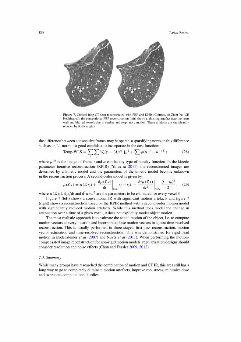
R88 Topical Review

Figure 7. Clinical lung CT scan reconstructed with FBP and KPIR (Courtesy of Zhou Yu (GEHealthcare)): the conventional FBP reconstruction (left) shows a ghosting artefact near the heartwall and blurred vessels due to cardiac and respiratory motion. These artefacts are significantlyreduced by KPIR (right).

the difference between consecutive frames may be sparse, a sparsifying norm on this differencesuch as an L1 norm is a good candidate to incorporate in the cost function:

Temp-WLS =$

t

$

i

Wi(yi ! [Aµ(t)]i)2 +

$

t

*(µ(t) ! µ(t+1)) (28)

where µ(t) is the image of frame t and * can be any type of penalty function. In the kineticparameter iterative reconstruction (KPIR) (Yu et al 2011), the reconstructed images aredescribed by a kinetic model and the parameters of the kinetic model become unknownin the reconstruction process. A second-order model is given by

µ(!x, t) = µ(!x, t0) + dµ(!x, t)dt

////t=t0

(t ! t0) + d2µ(!x, t)dt2

////t=t0

(t ! t0)2

2, (29)

where µ(!x, t0), dµ/dt and d2µ/dt2 are the parameters to be estimated for every voxel !x.Figure 7 (left) shows a conventional IR with significant motion artefacts and figure 7

(right) shows a reconstruction based on the KPIR method with a second-order motion modelwith significantly reduced motion artefacts. While this method does model the change inattenuation over a time of a given voxel, it does not explicitly model object motion.

The most realistic approach is to estimate the actual motion of the object, i.e. to computemotion vectors at every location and incorporate these motion vectors in a joint time-resolvedreconstruction. This is usually performed in three stages: first-pass reconstruction, motionvector estimation and time-resolved reconstruction. This was demonstrated for rigid headmotion in Bodensteiner et al (2007) and Nuyts et al (2011). When performing the motion-compensated image reconstruction for non-rigid motion models, regularization designs shouldconsider resolution and noise effects (Chun and Fessler 2009, 2012).

7.3. Summary

While many groups have researched the combination of motion and CT IR, this area still has along way to go to completely eliminate motion artefacts, improve robustness, minimize doseand overcome computational hurdles.

Topical Review R89

8. Supplemental data

Two movies are provided illustrating motion correction with phase weighting:

(i) Movie of a rabbit heart scanned with a flat-panel VCT system using an 18 s gantryperiod and reconstructed with the phase-weighted iterative reconstruction (PW-MLTR).An entire cardiac cycle is shown for each transaxial cross-section. This is repeated fora stack of transaxial cross-section at consecutive longitudinal positions. (available fromstacks.iop.org/PMB/58/R63/mmedia)

(ii) Movie of a rabbit heart scanned with a flat-panel VCT system using an 18 s gantry periodand reconstructed with PW-MLTR. An entire cardiac cycle is shown for each longitudinalcross-section. This is repeated for all longitudinal cross-sections containing the rotationaxis at consecutive angles. (available from stacks.iop.org/PMB/58/R63/mmedia)

Acknowledgments

BDM and JF are supported in part by the NIH grant R01-HL-098686. FB is supported by the3Binding PID Project, Dutch Economical Affairs. WZ was supported in part by the NIH grant2R01-CA-112163.

References

Alvarez R E and Macovski A 1976 Energy-selective reconstructions in x-ray computed tomography Phys. Med.Biol. 21 733–44

Andersen A H and Kak A C 1984 Simultaneous algebraic reconstruction technique (SART): a superior implementationof the ART algorithm Ultrasonic Imaging 6 81–94

Angel E et al 2009 Monte Carlo simulations to assess the effects of tube current modulation on breast dose formultidetector CT Phys. Med. Biol. 54 497–512

Badal A and Badano A 2009 Accelerating Monte Carlo simulations of photon transport in a voxelized geometry usinga massively parallel graphics processing unit Med. Phys. 36 4878–80

Badano A and Sempau J 2006 MANTIS: combined x-ray, electron and optical Monte Carlo simulations of indirectradiation imaging systems Phys. Med. Biol. 51 1545–62

Bae K T and Whiting B R 2001 CT data storage reduction by means of compressing projection data instead of images:feasibility study Radiology 219 850–5

Beekman F J, De Jong H W and Slijpen E T 1999 Efficient SPECT scatter calculation in non-uniform media usingcorrelated Monte Carlo simulation Phys. Med. Biol. 44 N183–92

Benson T M and De Man B K B 2010 Synthetic CT noise emulation in the raw data domain Proc. IEEE Nucl. Sci.Symp. Med. Imaging Conf. pp 3169–71

Benson T M and Gregor J 2006 Three-dimensional focus of attention for iterative cone-beam micro-CT reconstructionPhys. Med. Biol. 51 4533–46

Bertram M, Sattel T, Hohmann S and Wiegert J 2008 Monte-Carlo scatter correction for cone-beam computedtomography with limited scan field-of-view Proc. SPIE 6913 69131Y

Bertram M, Wiegert J and Rose G 2005 Potential of software-based scatter corrections in cone-beam volume CTProc. SPIE 5745 259–70

Bertram M, Wiegert J and Rose G 2006 Scatter correction for cone-beam computed tomography using simulatedobject models Proc. SPIE 61421 61421C

Bian J, Siewerdsen J H, Han X, Sidky E Y, Prince J L, Pelizzari C A and Pan X 2010 Evaluation of sparse-viewreconstruction from flat-panel-detector cone-beam CT Phys. Med. Biol. 55 6575–99

Bian J, Wang J, Han X, Sidky E Y, Shao L and Pan X 2013 Optimization-based image reconstruction from sparse-viewdata in offset-detector CBCT Phys. Med. Biol. 58 205–30

Blevis I M, Hunt D C and Rowlands J A 1998 X-ray imaging using amorphous selenium: Determination of Swankfactor by pulse height spectroscopy Med. Phys. 25 638–41

Bodensteiner C, Darolti C, Schumacher H, Matthaus L and Schweikard A 2007 Motion and positional error correctionfor cone beam 3D-reconstruction with mobile C-arms Int. Conf. on Medical Image Computing and Computer-Assisted Intervention (Lecture Notes in Computer Science 4791) pp 177–85

R90 Topical Review

Bootsma G, Verhaegen F and Jaffray D 2012 SU-F-BRCD-04: efficient scatter distribution estimation and correctionin CBCT using concurrent Monte Carlo fitting Med. Phys. 39 3856

Bowsher J E, Tornai M P, Peter J, Gonzalez Trotter D E, Krol A, Gilland D R and Jaszczak R J 2002 Modeling theaxial extension of a transmission line source within iterative reconstruction via multiple transmission sourcesIEEE. Trans. Med. Imaging 21 200–15

Boyd D P 1979 Status of diagnostic x-ray CT: IEEE Trans. Nucl. Sci. 26 2835–9Brankov J G, Yang Y and Wernick M N 2004 Tomographic image reconstruction based on a content-adaptive mesh

model IEEE Trans. Med. Imaging 23 202–12Brankov J G, Yang Y and Wernick M N 2005 Spatiotemporal processing of gated cardiac SPECT images using

deformable mesh modeling Med. Phys. 32 2839–49Brooks R A and Di Chiro G 1976 Beam-hardening in x-ray reconstructive tomography Phys. Med. Biol. 21 390–8Browne J A, Boone J M and Holmes T J 1995 Maximum-likelihood x-ray computed-tomography finite-beamwidth

considerations Appl. Opt. 34 5199–209Byrne C L 2008 Applied Iterative Methods (Wellesley, MA: A K Peters)Cai W, Ning R and Conover D 2011 Scatter correction for clinical cone beam CT breast imaging based on breast

phantom studies J. X-Ray Sci. Technol. 19 91–109Carmi R, Shapiro O and Braunstein D 2004 Resolution enhancement of x-ray CT by spatial and temporal MLEM

deconvolution correction IEEE Nucl. Sci. Symp. Med. Imaging Conf. Rec. vols 1–7 pp 2765–8Carvalho B A and Herman G T 2007 Low-dose, large-angled cone-beam helical CT data reconstruction using algebraic

reconstruction techniques Image Vis. Comput. 25 78–94Chun S Y and Fessler J A 2009 Joint image reconstruction and nonrigid motion estimation with a simple penalty that

encourages local invertibility Proc. SPIE 7258 72580UChun S Y and Fessler J A 2012 Spatial resolution properties of motion-compensated image reconstruction methods

IEEE Trans. Med. Imaging 31 1413–25Clackdoyle R and Defrise M 2010 Tomographic reconstruction in the 21st century IEEE Signal Process. Mag. 7 60–80Clinthorne N H 1994 A constrained dual-energy reconstruction method for material-selective transmission

tomography Nucl. Instrum. Methods Phys. Res. A 353 347–8Colijn A P and Beekman F J 2004 Accelerated simulation of cone beam x-ray scatter projections IEEE Trans. Med.

Imaging 23 584–90Colijn A P, Zbijewski W, Sasov A and Beekman F J 2004 Experimental validation of a rapid Monte Carlo based

micro-CT simulator Phys. Med. Biol. 49 4321–33De Man B 2001 Iterative reconstruction for reduction of metal artifacts in computed tomography PhD dissertation

KU Leuven, BelgiumDe Man B and Basu S 2004 Distance-driven projection and backprojection in three dimensions Phys. Med.

Biol. 49 2463–75De Man B, Edic P and Basu S 2003 Phase-weighted sparse-view iterative reconstruction for cardiac CT European

College of Radiology Vienna, AustriaDe Man B, Edic P M and Basu S 2005 An iterative algorithm for time-resolved reconstruction of a CT scan of

a beating heart 8th Int. Meeting on Fully Three-Dimensional Image Construction in Radiology and NuclearMedicine pp 356–9

De Man B and Fessler J A 2010 Statistical iterative reconstruction for x-ray computed tomography BiomedicalMathematics: Promising Directions in Imaging, Therapy Planning and Inverse Problems ed Y Censor, M Jianand G Wang (Madison, WI: Medical Physics Publishing) pp 113–40

De Man B, Nuyts J, Dupont P and Marchal G 2000 Reduction of metal steak artifacts in x-ray computed tomographyusing a transmission maximum a posteriori algorithm IEEE Trans. Nucl. Sci. 47 977–81

De Man B, Nuyts J, Dupont P, Marchal G and Suetens P 2001 An iterative maximum-likelihood polychromaticalgorithm for CT IEEE Trans. Med. Imaging 20 999–1008

De Man B et al 2007 CatSim: a new computer assisted tomography simulation environment Proc. SPIE 6510 65102GDepypere M, Nuyts J, van Gastel N, Carmeliet G, Maes F and Suetens P 2011 An iterative dual energy CT

reconstruction method for a K-edge contrast material Proc. SPIE 7961 79610MElbakri I A and Fessler J A 2002 Statistical image reconstruction for polyenergetic x-ray computed tomography IEEE

Trans. Med. Imaging 21 89–99Elbakri I A and Fessler J A 2003a Segmentation-free statistical image reconstruction for polyenergetic x-ray computed

tomography with experimental validation Phys. Med. Biol. 48 2453–77Elbakri I A and Fessler J A 2003b Efficient and accurate likelihood for iterative image reconstruction in x-ray

computed tomographyProc. SPIE 5032 1839–50Endo M, Tsunoo T, Nakamori N and Yoshida K 2001 Effect of scattered radiation on image noise in cone beam CT

Med. Phys. 28 469–74

Topical Review R91

Evans J D, Whiting B R, Politte D G, O’Sullivan J A, Klahr P F and Williamson J F 2013 Experimental implementationof a polyenergetic statistical reconstruction algorithm for a commercial fan-beam CT scanner Phys. Med.at press (doi:10.1016/j.ejmp.2012.12.005)

Feng B, Fessler J A and King M A 2006 Incorporation of system resolution compensation (RC) in the ordered-subsettransmission (OSTR) algorithm for transmission imaging in SPECT IEEE Trans. Med. Imaging 25 941–9

Fessler J A 1994 Penalized weighted least-squares image reconstruction for positron emission tomography IEEETrans. Med. Imaging 13 290–300

Fessler J A, Elbakri I, Sukovic P and Clinthorne N H 2002 Maximum-likelihood dual-energy tomographic imagereconstruction Proc. SPIE 4684 38–49

Forthmann P, Kohler T, Begemann P G C and Defrise M 2007 Penalized maximum-likelihood sinogram restorationfor dual focal spot computed tomography Phys. Med. Biol. 52 4513–23

Frush D P, Slack C C, Hollingsworth C L, Bisset G S, Donnelly L F, Hsieh J, Lavin-Wensell T and Mayo J R2002 Computer simulated radiation dose reduction for abdominal multidetector CT of pediatric patients Am. J.Roentgenol. 179 1107–13

Gies M, Kalender W A, Wolf H and Suess C 1999 Dose reduction in CT by anatomically adapted tube currentmodulation: I. Simulation studies Med. Phys. 26 2235–47

Ginzburg A and Dick C E 1993 Image information transfer properties of x-ray intensifying screens in the energyrange from 17 to 320 keV Med. Phys. 20 1013–21

Glover G H 1982 Compton scatter effects in CT reconstructions Med. Phys. 9 860–7Glover G H and Pelc N J 1980 Nonlinear partial volume artifacts in x-ray computed tomography Med. Phys. 7 238–48Goertzen A L, Beekman F J and Cherry S R 2002 Effect of phantom voxelization in CT simulations Med.

Phys. 29 492–8Gordon R, Bender R and Herman G T 1970 Algebraic reconstruction techniques (ART) for three-dimensional electron

microscopy and x-ray photography J. Theor. Biol. 29 471–81Greess H, Wolf H, Baum U, Lell M, Pirkl M, Kalender W and Bautz W A 2000 Dose reduction in computed

tomography by attenuation-based on-line modulation of tube current: evaluation of six anatomical regions Eur.Radiol. 10 391–4

Hamelin B, Goussard Y and Dussault J-P 2007 Penalized-likelihood region-of-interest CT reconstruction bylocal object supersampling Proc. 29th Annu. Int. Conf. on IEEE Engineering in Medicine and BiologySociety pp 739–42

Hamelin B, Goussard Y, Dussault J-P, Beaudoin G and Soulez G 2010 Design of iterative ROI transmissiontomography reconstruction procedures and image quality analysis Med. Phys. 37 4577–89

Heismann B J, Schmidt B T and Flohr T 2012 Spectral Computed Tomography (Bellingham WA: SPIE OpticalEngineering Press)

Herman G T 1979 Correction for beam hardening in computed tomography Phys. Med. Biol. 24 81–106Herman G T and Davidi R 2008 Image reconstruction from a small number of projections Inverse Problems 24 045011Herman G T and Trivedi S S 1983 A comparative study of two postreconstruction beam hardening correction methods

IEEE Trans. Med. Imaging 2 128–35Hsieh J, Molthen R C, Dawson C A and Johnson R H 2000 An iterative approach to the beam hardening correction

in cone beam CT Med. Phys. 27 23–29Hurwitz L M, Yoshizumi T T, Goodman P C, Nelson R C, Toncheva G, Nguyen G B, Lowry C and Anderson-Evans C

2009 Radiation dose savings for adult pulmonary embolus 64-MDCT using bismuth breast shields, lower peakkilovoltage and automatic tube current modulation Am. J. Roentgenol. 192 244–53

Iatrou M, De Man B, Khare K and Benson T M 2007 A 3D study comparing filtered backprojection, weighted leastsquares and penalized weighted least squares for CT reconstruction Proc. IEEE Nucl. Sci. Symp. Med. ImagingConf. vol 4 2639–43

Isola A A, Grass M and Niessen W J 2010 Fully automatic nonrigid registration-based local motion estimation formotion-corrected iterative cardiac CT reconstruction Med. Phys. 37 1093–109

Isola A A, Ziegler A, Koehler T, Niessen W J and Grass M 2008 Motion-compensated iterative cone-beam CT imagereconstruction with adapted blobs as basis functions Phys. Med. Biol. 53 6777–97

Jarry G, Graham S A, Jaffray D A, Moseley D J and Verhaegen F 2006 Scatter correction for kilovoltage cone-beamcomputed tomography (CBCT) images using Monte Carlo simulations Proc. SPIE 6142 14254

Jin J Y, Ren L, Liu Q, Kim J, Wen N, Guan H, Movsas B and Chetty I J 2010 Combining scatter reduction andcorrection to improve image quality in cone-beam computed tomography (CBCT) Med. Phys. 37 5634–44

Johns P C and Yaffe M 1982 Scattered radiation in fan beam imaging-systems Med. Phys. 9 231–9Johnston S M, Johnson G A and Badea C T 2012 Temporal and spectral imaging with micro-CT Med.

Phys. 39 4943–58Jorgensen B 1987 Exponential dispersion models J. R. Stat. Soc. B 49 127–62 (available at www.jstor.org/

stable/2345415)

R92 Topical Review

Joseph P M 1982 An improved algorithm for reprojecting rays through pixel images IEEE Trans. Med.Imaging 1 192–6

Joseph P M and Ruth C 1997 A method for simultaneous correction of spectrum hardening artifacts in CT imagescontaining both bone and iodine Med. Phys. 24 1629–34

Joseph P M and Spital R D 1978 A method for correcting bone induced artifacts in computed tomography scannersJ. Comput. Assist. Tomogr. 2 100–8

Joseph P M and Spital R D 1981 The exponential edge-gradient effect in x-ray computed tomography Phys. Med.Biol. 26 473–87

Joseph P M and Spital R D 1982 The effects of scatter in X-ray computed-tomography Med. Phys. 9 464–72Kaipio J and Somersalo E 2007 Statistical inverse problems: discretization, model reduction and inverse crimes

J. Comput. Appl. Math. 198 493–504Kalender W A 2006 X-ray computed tomography Phys. Med. Biol. 51 R29–43Kalender W A and Kyriakou Y 2007 Flat-detector computed tomography (FD-CT) Eur. Radiol. 17 2767–79Kalender W A, Wolf H and Suess C 1999 Dose reduction in CT by anatomically adapted tube current modulation: II.

Phantom measurements Med. Phys. 26 2248–53Karmazyn B, Frush D P, Applegate K E, Maxfield C, Cohen M D and Jones R P 2009 CT with a computer-simulated

dose reduction technique for detection of pediatric nephroureterolithiasis: comparison of standard and reducedradiation doses Am. J. Roentgenol. 192 143–9

Katsevich A 2002 Analysis of an exact inversion algorithm for spiral cone-beam CT Phys. Med. Biol. 47 2583–97Knoll G F 2000 Radiation Detection and Measurement 3rd edn (New York: Wiley)Kunze H, Stierstorfer K and Haerer W 2005 Year. Pre-processing of projections for iterative reconstruction 8th Int.

Meeting on Fully Three-Dimensional Image Reconstruction in Radiology and Nuclear Medicine pp 84–87Kwan A L, Boone J M and Shah N 2005 Evaluation of x-ray scatter properties in a dedicated cone-beam breast CT

scanner Med. Phys. 32 2967–75Kyprianou L S, Rudin S, Bednarek D R and Hoffmann K R 2005 Generalizing the MTF and DQE to include

x-ray scatter and focal spot unsharpness: application to a new microangiographic system Med. Phys.32 613–26

Kyriakou Y, Meyer E, Prell D and Kachelriess M 2010 Empirical beam hardening correction (EBHC) for CT Med.Phys. 37 5179–87

Kyriakou Y, Riedel T and Kalender W A 2006 Combining deterministic and Monte Carlo calculations for fastestimation of scatter intensities in CT Phys. Med. Biol. 51 4567–86

Lange K and Carson R 1984 EM reconstruction algorithms for emission and transmission tomography J. Comput.Assist. Tomogr. 8 306–16

La Riviere P J, Bian J and Vargas P A 2006 Penalized-likelihood sinogram restoration for computed tomographyIEEE. Trans. Med. Imaging 25 1022–36

La Riviere P J and Vargas P 2008 Correction for resolution nonuniformities caused by anode angulation in computedtomography IEEE Trans. Med. Imaging 27 1333–41

Lasio G M, Whiting B R and Williamson J F 2007 Statistical reconstruction for x-ray computed tomography usingenergy-integrating detectors Phys. Med. Biol. 52 2247–66

Lee H, Xing L, Lee R and Fahimian B P 2012 Scatter correction in cone-beam CT via a half beam blocker techniqueallowing simultaneous acquisition of scatter and image information Med. Phys. 39 2386–95

Lei T 2011 Statistics of Medical Imaging (Boca Raton, FL: Chapman and Hall/CRC)Lewitt R M 1990 Multidimensional digital image representations using generalized Kaiser–Bessel window functions

J. Opt. Soc. Am. A 7 1834–46Lewitt R M 1992 Alternatives to voxels for image representation in iterative reconstruction algorithms Phys. Med.

Biol. 37 706–16Li H, Mohan R and Zhu X R 2008 Scatter kernel estimation with an edge-spread function method for cone-beam

computed tomography imaging Phys. Med. Biol. 53 6729–48Little K J and La Riviere P J 2012 An algorithm for modeling non-linear system effects in iterative CT reconstruction

IEEE Nucl. Sci. Symp. Med. Imaging Conf. Rec. pp 2174–7Liu X, Shaw C, Altunbas M and Wang T 2005 A scanning sampled measurement (SSM) technique for scatter

measurement and correction in cone beam breast CT Med. Phys. 32 2093Liu X, Yu L, Primak A N and McCollough C H 2009 Quantitative imaging of element composition and mass fraction

using dual-energy CT: three-material decomposition Med. Phys. 36 1602–9Long Y and Fessler J A 2012 Multi-material decomposition using statistical image reconstruction in x-ray CT Proc.

2nd Int. Mtg. on image formation in X-ray CT pp 413–6Long Y, Fessler J A and Balter J M 2010 3D forward and back-projection for x-ray CT using separable footprints

IEEE Trans. Med. Imaging 29 1839–50

Topical Review R93

Long Y, Fessler J A and Balter J M 2011 Two-material decomposition from a single CT scan using statistical imagereconstruction Proc. Joint AAPM Conf. Meeting p 3810

Love L A and Kruger R A 1987 Scatter estimation for a digital radiographic system using convolution filtering Med.Phys. 14 178–85

Lucy L B 1974 An iterative technique for the rectification of observed distributions Astron. J. 79 745–54Ma J, Liang Z, Fan Y, Liu Y, Huang J, Chen W and Lu H 2012 Variance analysis of x-ray CT sinograms in the

presence of electronic noise background Med. Phys. 39 4051–65Maass C, Meyer E and Kachelriess M 2011 Exact dual energy material decomposition from inconsistent rays (MDIR)

Med. Phys. 38 691–700Mainegra-Hing E and Kawrakow I 2010 Variance reduction techniques for fast Monte Carlo CBCT scatter correction

calculations Phys. Med. Biol. 55 4495–507Maltz J S, Gangadharan B, Bose S, Hristov D H, Faddegon B A, Paidi A and Bani-Hashemi A R 2008 Algorithm for x-

ray scatter, beam-hardening, and beam profile correction in diagnostic (kilovoltage) and treatment (megavoltage)cone beam CT IEEE Trans. Med. Imaging 27 1791–810

Massoumzadeh P, Don S, Hildebolt C F, Bae K T and Whiting B R 2009 Validation of CT dose-reduction simulationMed. Phys. 36 174–89

Matej S and Lewitt RM 1996 Practical considerations for 3-D image reconstruction using spherically symmetricalvolume elements IEEE. Trans. Med. Imaging 15 68–78

Mayo J R, Whittall K P, Leung A N, Hartman T E, Park C S, Primack S L, Chambers G K, Limkeman M K, Toth T Land Fox S H 1997 Simulated dose reduction in conventional CT: validation study Radiology 202 453–7

McDavid W D, Waggener R G, Payne W H and Dennis M J 1975 Spectral effects on three-dimensional reconstructionfrom x-rays Med. Phys. 2 321–4

Mendonca P R S, Bhotika R, Thomsen B W, Licato P E and Joshi M C 2010 Multi-material de-composition ofdual-energy CT dataProc. SPIE 7622 76221W

Meyer M, Kalender W A and Kyriakou Y 2010 A fast and pragmatic approach for scatter correction in flat-detectorCT using elliptic modeling and iterative optimization Phys. Med. Biol. 55 99–120

Michielsen K, Van Slambrouck K, Jerbko A and Nuyts J 2013 Patchwork reconstruction with resolution modelingfor digital breast tomosynthesis Med. Phys. 40 031105

Neitzel U 1992 Grids or air gaps for scatter reduction in digital radiography: a model calculation Med. Phys. 19 475–81Neukirchen C, Giordano M and Wiesner S 2010 An iterative method for tomographic x-ray perfusion estimation in a

decomposition model-based approach Med. Phys. 37 6125–41Nien H and Fessler J A 2013 Splitting-based statistical x-ray CT image reconstruction with blind gain correction

Proc. SPIE. 8668 8668–53Ning R, Tang X Y and Conover D 2004 X-ray scatter correction algorithm for cone beam CT imaging Med.

Phys. 31 1195–202Niu T, Al-Basheer A and Zhu L 2012 Quantitative cone-beam CT imaging in radiation therapy using planning CT as

a prior: first patient studies Med. Phys. 39 1991–2000Niu T and Zhu L 2011 Scatter correction for full-fan volumetric CT using a stationary beam blocker in a single full

scan Med. Phys. 38 6027–38Noo F, Pack J and Heuscher D 2003 Exact helical reconstruction using native cone-beam geometries Phys. Med.

Biol. 48 3787–818Nuyts J, De Man B, Dupont P, Defrise M, Suetens P and Mortelmans L 1998 Iterative reconstruction for helical CT:

a simulation study Phys. Med. Biol. 43 729–37Nuyts J, Kim J and Fulton R 2011 Iterative CT reconstruction with correction for known rigid motion 11th Int.

Meeting on Fully Three-Dimensional Image Reconstruction in Radiology and Nuclear Medicine pp 132–35O’Sullivan J A and Benac J 2003 Alternating minimization multigrid algorithms for transmission tomography Proc.

SPIE 5299 216–21O’Sullivan J A and Benac J 2007 Alternating minimization algorithms for transmission tomography IEEE Trans.

Med. Imaging 26 283–97Pack J D, Noo F and Kudo H 2004 Investigation of saddle trajectories for cardiac CT imaging in cone-beam geometry

Phys. Med. Biol. 49 2317–36Pan X, Sidky E Y and Vannier M 2009 Why do commercial CT scanners still employ traditional, filtered back-

projection for image reconstruction? Inverse Problems 25 123009Parker D L 1982 Optimal short scan convolution reconstruction for fanbeam CT Med. Phys. 9 254–7Poludniowski G, Evans P M, Hansen V N and Webb S 2009 An efficient Monte Carlo-based algorithm for scatter

correction in keV cone-beam CT Phys. Med. Biol. 54 3847–64Rathee S, Koles Z J and Overton T R 1992 Image restoration in computed tomography: the spatially invariant point

spread function IEEE Trans. Med. Imaging 11 530–8

R94 Topical Review

Richardson W H 1972 Bayesian-based iterative method of image restoration J. Opt. Soc. Am. 62 55–59Ritchie C J, Godwin D, Crawford C R, Stanford W, Anno H and Kim Y 1992 Minimum scan speeds for suppression

of motion artifacts in CT Radiology 185 37–42Ruhrnschopf E P and Klingenbeck K 2011a A general framework and review of scatter correction methods in x-ray

cone-beam computerized tomography: part 1. Scatter compensation approaches Med. Phys. 38 4296–311Ruhrnschopf E P and Klingenbeck K 2011b A general framework and review of scatter correction methods in cone

beam CT: part 2. Scatter estimation approaches Med. Phys. 38 5186–99Sauer K and Bouman C 1993 A local update strategy for iterative reconstruction from projections IEEE Trans. Signal

Process. 41 534–48Sechopoulos I 2012 X-ray scatter correction method for dedicated breast computed tomography Med.

Phys. 39 2896–903Seibert J A and Boone J M 1988 X-ray scatter removal by deconvolution Med. Phys. 15 567–75Semerci O and Miller E L 2012 A parametric level set approach to simultaneous object identification and background

reconstruction for dual energy computed tomography IEEE Trans. Image Process. 21 2917–34Shikhaliev P M 2005 Beam hardening artefacts in computed tomography with photon counting, charge integrating

and energy weighting detectors: a simulation study Phys. Med. Biol. 50 5813–28Siddon R L 1985 Fast calculation of the exact radiological path for a three-dimensional CT array Med. Phys. 12 252–5Sidky E Y, Kao C-M and Pan X 2006 Accurate image reconstruction from few-views and limited-angle data in

divergent-beam CT J. X-Ray Sci. Technol. 14 119–39Sidky E Y and Pan X 2008 Image reconstruction in circular cone-beam computed tomography by constrained,

total-variation minimization Phys. Med. Biol. 53 4777–807Siewerdsen J H, Antonuk L E, El-Mohri Y, Yorkston J, Huang W, Boudry J M and Cunningham I A 1997 Empirical

and theoretical investigation of the noise performance of indirect detection, active matrix flat-panel imagers(AMFPIs) for diagnostic radiology Med. Phys. 24 71–89

Siewerdsen J H, Daly M J, Bakhtiar B, Moseley D J, Richard S, Keller H and Jaffray D A 2006 A simple, direct methodfor x-ray scatter estimation and correction in digital radiography and cone-beam CT Med. Phys. 33 187–97

Siewerdsen J H and Jaffray D A 2001 Cone-beam computed tomography with a flat-panel imager: magnitude andeffects of x-ray scatter Med. Phys. 28 220–31

Siewerdsen J H, Moseley D J, Bakhtiar B, Richard S and Jaffray D A 2004 The influence of antiscatter grids onsoft-tissue detectability in cone-beam computed tomography with flat-panel detectors Med. Phys. 31 3506–20

Snyder D L, Hammoud A M and White R L 1993 Image recovery from data acquired with a charge-coupled-devicecamera J. Opt. Soc. Am. A 10 1014–23

Snyder D L, Helstrom C W, Lanterman A D, Faisal M and White R L 1995 Compensation for readout noise in CCDimages J. Opt. Soc. Am. A 12 272–83

Snyder D L and Miller M I 1985 The use of sieves to stabilize images produced with the EM algorithm for emissiontomography IEEE Trans. Nucl. Sci. NS-32 3864–72

Snyder D L, Miller M I, Thomas L J and Politte D G 1987 Noise and edge artifacts in maximum-likelihoodreconstructions for emission tomography IEEE Trans. Med. Imaging 6 228–38

Spanier J and Gelbard E M 1969 Monte Carlo Principles and Neutron Transport Problems (Reading, MA: Addison-Wesley)

Srivastava S, Cammin J, Fung G S K, Tsui B M W and Taguchi K 2012 Spectral response compensation for photon-counting clinical x-ray CT using sinogram restoration Proc. SPIE 8313 831311

Stayman J W, Dang H, Otake Y, Zbijewski W, Noble J, Dawant B, Labadie R F, Carey J P and Siewerdsen J H 2013Overcoming nonlinear partial volume effects in known-component reconstruction of cochlear implants Proc.SPIE 8668 86681L

Sukovic P and Clinthorne N H 2000 Penalized weighted least-squares image reconstruction for dual energy x-raytransmission tomography IEEE Trans. Med. Imaging 19 1075–81

Sun M and Star-Lack J M 2010 Improved scatter correction using adaptive scatter kernel superposition Phys. Med.Biol. 55 6695–720

Swank R K 1973 Absorption and noise in x-ray phosphors J. Appl. Phys. 44 4199–203Taguchi K, Srivastava S, Tang Q, Caffo B S, Iwanczyk J S, Hartsough N E, Barber W C and Cammin J 2012

Pulse pileup statistics for energy sensitive photon counting detectors with pulse height analysis Proc.SPIE 8313 83130Z

Takahashi T, Itoh H, Shimada T and Takeuchi H 1990 Design of integrated radiation detectors with a-si photodiodeson ceramic scintillators for use in x-ray computed tomography IEEE Trans. Nucl. Sci. 37 1478–82

Tam K C, Samarasekera S and Sauer F 1998 Exact cone beam CT with a spiral scan Phys. Med. Biol. 43 1015–24Tang J, Hsieh H and Chen G-H 2010 Temporal resolution improvement in cardiac CT using PICCS (TRI-PICCS):

performance studies Med. Phys. 37 4377–88

Topical Review R95

Thibault J-B, Bouman C A, Sauer K D and Hsieh J 2006 A recursive filter for noise reduction in statistical iterativetomographic imaging Proc. SPIE 6065 60650X

Thibault J B, Sauer K D, Bouman C A and Hsieh J 2007 A three-dimensional statistical approach to improved imagequality for multislice helical CT Med. Phys. 34 4526–44

Thibault J-B, Yu Z, Sauer K, Bouman C and Hsieh J 2007 Correction of gain fluctuations in iterative tomographicimage reconstruction Proc. Int. Meeting on Fully Three-Dimensional Image Reconstruction in Radiology andNuclear Medicine pp 112–5

Toth T L, Cesmeli E, Ikhlef A and Horiuchi T 2005 Image quality and dose optimization using novel x-ray sourcefilters tailored to patient size Proc. SPIE 5745 283–91

Van Slambrouck K and Nuyts J 2012 Metal artifact reduction in computed tomography using local models in animage block-iterative scheme Med. Phys. 39 7080–93

Wang A S, Feng C and Pelc N J 2012 Image-based synthetic CT: simulating arbitrary low dose single and dual energyprotocols from dual energy images Proc. SPIE 8313 83131G

Wang G, Lin T-H and Cheng P C 1993 A general cone-beam reconstruction algorithm IEEE Trans. Med.Imaging 12 486–96

Wang G, Vannier M W, Skinner M W, Cavalcanti M G P and Harding G W 1998 Spiral CT image deblurring forcochlear implantation IEEE Trans. Med. Imaging 17 251–62

Wang J, Mao W and Solberg T 2010 Scatter correction for cone-beam computed tomography using moving blockerstrips: a preliminary study Med. Phys. 37 5792–800

Whiting B R 2002 Signal statistics in x-ray computed tomography Proc. SPIE 4682 53–60Whiting B R, Massoumzadeh P, Earl O A, O’Sullivan J A, Snyder D L and Williamson J F 2006 Properties of

preprocessed sinogram data in x-ray computed tomography Med. Phys. 33 3290–303Xiao J, Verzijlbergen F J, Viergever M A and Beekman F J 2010 Small field-of-view dedicated cardiac SPECT

systems: impact of projection truncation Eur. J. Nucl. Med. Mol. Imaging 37 528–36Xu D, Langan D A, Wu X, Pack J D, Benson T M, Tkaczky J E and Schmitz A M 2009 Dual energy CT via fast kVp

switching spectrum estimation Proc. SPIE 7258 72583TXu J, Frey E C, Taguchi K and Tsui B M W 2007 A Poisson likelihood iterative reconstruction algorithm for material

decomposition in CT Proc. SPIE 6510 65101ZXu J and Tsui B M W 2007 A compound Poisson maximum-likelihood iterative reconstruction algorithm for x-ray

CT Proc. Int. Meeting on Fully Three-Dimensional Image Reconstruction in Radiology and Nuclear Medicinepp 108–11

Xu J and Tsui B M W 2009 Electronic noise modeling in statistical iterative reconstruction IEEE Trans. ImageProcess. 18 1228–38

Xu Q et al 2012 Image reconstruction for hybrid true-color micro-CT IEEE Trans. Biomed. Eng. 59 1711–9Yan C H, Whalen R T, Beaupre G S, Yen S Y and Napel S 2000 Reconstruction algorithm for polychromatic CT

imaging: application to beam hardening correction IEEE Trans. Med. Imaging 19 1–11Yang K, Burkett G and Boone J M 2012 An object-specific and dose-sparing scatter correction approach for a

dedicated cone-beam breast CT system using a parallel-hole collimator Proc. SPIE 8313 831303Yao W and Leszczynski K W 2009 An analytical approach to estimating the first order scatter in heterogeneous

medium: II. A practical application Med. Phys. 36 3157–67Yu D F and Fessler J A 2000 Mean and variance of singles photon counting with deadtime Phys. Med. Biol. 45 2043–56Yu D F and Fessler J A 2002 Mean and variance of coincidence photon counting with deadtime Nucl. Instrum.

Methods Phys. Res. A 488 362–74Yu D F, Fessler J A and Ficaro E P 2000 Maximum-likelihood transmission image reconstruction for overlapping

transmission beams IEEE Trans. Med. Imaging 19 1094–105Yu H and Wang G 2012 Finite detector based projection model for high spatial resolution J. X-Ray Sci. Technol.

20 229–38Yu Z, Thibault J-B, Wang J, Bouman C A and Sauer K D 2011 Kinetic model for motion compensation in computed

tomography 11th Int. Meeting on Fully Three-Dimensional Image Reconstruction in Radiology and NuclearMedicine pp 466–69

Zabic S, Wang Q and Brown K M 2012 A low-dose simulation tool Proc. 2nd Int. Meeting on Image Formation inX-Ray CT pp 61–65

Zbijewski W and Beekman F J 2004a Characterization and suppression of edge and aliasing artefacts in iterativex-ray CT reconstruction Phys. Med. Biol. 49 145–57

Zbijewski W and Beekman F J 2004b Suppression of intensity transition artifacts in statistical x-ray computertomography reconstruction through radon inversion initialization Med. Phys. 31 62–69

Zbijewski W and Beekman F J 2006a Comparison of methods for suppressing edge and aliasing artefacts in iterativex-ray CT reconstruction Phys. Med. Biol. 51 1877–89

R96 Topical Review

Zbijewski W and Beekman F J 2006b Efficient Monte Carlo based scatter artifact reduction in cone-beam micro-CTIEEE Trans. Med. Imaging 25 817–27

Zbijewski W, Sisniega A, Vaquero J J, Muhit A, Packard N, Senn R, Yang D, Yorkston J, Carrino J Aand Siewerdsen J H 2012 Dose and scatter characteristics of a novel cone beam CT system for musculoskeletalextremities Proc. SPIE 8313 8313–18

Zeng K, De Man B and Thibault J 2009a Correction of iterative reconstruction artifacts in helical cone-beam CT 10thInt. Conf. on Fully Three-Dimensional Reconstruction in Radiology and Nuclear Medicine pp 242–45

Zeng K, De Man B, Thibault J B, Yu Z, Bouman C and Sauer K 2009b Spatial resolution enhancement in CT iterativereconstruction IEEE Nucl. Sci. Symp. Med. Imaging Conf. Rec. pp 3748–51

Zhou J and Qi J 2011 Fast iterative image reconstruction using sparse matrix factorization with GPU accelerationProc. SPIE 7961 79610K

Zhu L, Bennett N R and Fahrig R 2006 Scatter correction method for x-ray CT using primary modulation: theory andpreliminary results IEEE Trans. Med. Imaging 25 1573–87

Zhu L, Strobel N and Fahrig R 2005 X-ray scatter correction for cone-beam CT using moving blocker array Proc.SPIE 5745 251–8

Ziegler A, Kohler T, Nielsen T and Proksa R 2006 Efficient projection and backprojection scheme for sphericallysymmetric basis functions in divergent beam geometry Med. Phys. 33 4653–63

Ziegler A, Nielsen T and Grass M 2008 Iterative reconstruction of a region of interest for transmission tomographyMed. Phys. 35 1317–27

Zou Y and Silver M D 2008 Analysis of fast kV-switching in dual energy CT using a pre-reconstruction decompositiontechnique Proc. SPIE 6913 691313