MODELLING THE EXTRACTION OF SUGAR FROM … Modelling the extraction of sugar from sugar cane in a di...

MODELLING THE EXTRACTION OF SUGAR

FROM SUGAR CANE IN A DIFFUSER

C. Breward∗, G. Hocking† , H. Ockendon‡ , C. Please§

and D. Schwendeman¶

Study group participants

A. Adolinline, C. Breward, R. Ferdinand, B. Florio, N. Fowkes,G. Hocking, A. Hutchinson, M. Khalique, D.P. Mason, H. Ockendon,

C. Please and M. Rademeyer

Industry representatives

Richard Loubser and Steve Davis

Abstract

Discrete and continuous mathematical models are constructed for the flowof sugarcane and juice through a sugar diffuser. The models describe howthe concentration of sugar in the juice increases during the process. The flowthrough the sugar cane in the diffuser is analysed. It is found that the fluidmoves downwards with constant velocity. The injection of tracer on one of thejets is modelled. The diffusivity of the tracer is different for the direction of flowand across the flow. The model is able to reproduce the behaviour observedin tracer experiments. A cavitation mechanism is investigated for creating dryregions in voids in the sugar cane. It is shown that the voids occur when the

∗Oxford Centre for Collaborative Applied Mathematics, University of Oxford, Oxford, UnitedKingdom, email: [email protected]†School of Chemical and Mathematical Sciences, Murdoch University, Perth, Western Australia,

Australia, email: [email protected]‡Oxford Center for Industrial and Applied Mathematics, University of Oxford, Oxford, United

Kingdom, email: [email protected]§Oxford Centre for Collaborative Applied Mathematics, University of Oxford, Oxford, United

Kingdom, email: [email protected]¶Oxford Centre for Collaborative Applied Mathematics, University of Oxford, Oxford, United

Kingdom, email: [email protected]

31

32 Modelling the extraction of sugar from sugar cane in a diffuser

permeability varies with depth in a way to produce regions of negative pressure.Their existence depends on the variation in the permeability through the wholedepth but especially on regions of low permeability away from the bottom ofthe bed.

1 Introduction

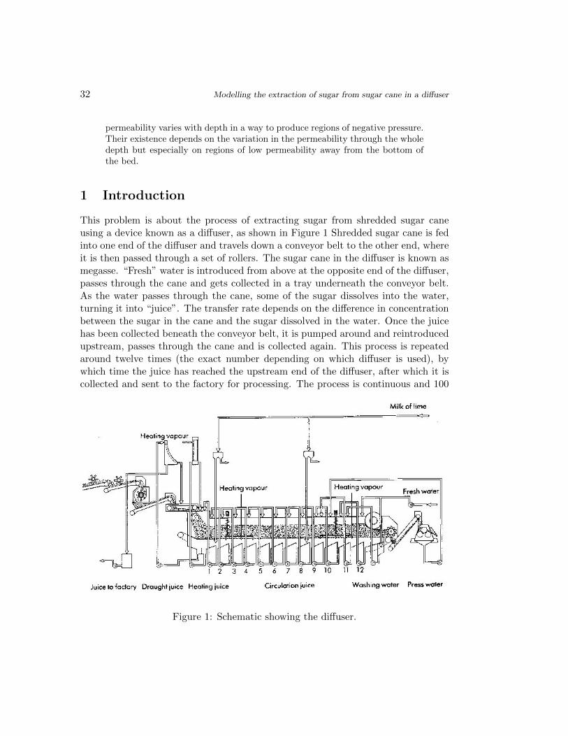
This problem is about the process of extracting sugar from shredded sugar caneusing a device known as a diffuser, as shown in Figure 1 Shredded sugar cane is fedinto one end of the diffuser and travels down a conveyor belt to the other end, whereit is then passed through a set of rollers. The sugar cane in the diffuser is known asmegasse. “Fresh” water is introduced from above at the opposite end of the diffuser,passes through the cane and gets collected in a tray underneath the conveyor belt.As the water passes through the cane, some of the sugar dissolves into the water,turning it into “juice”. The transfer rate depends on the difference in concentrationbetween the sugar in the cane and the sugar dissolved in the water. Once the juicehas been collected beneath the conveyor belt, it is pumped around and reintroducedupstream, passes through the cane and is collected again. This process is repeatedaround twelve times (the exact number depending on which diffuser is used), bywhich time the juice has reached the upstream end of the diffuser, after which it iscollected and sent to the factory for processing. The process is continuous and 100

Figure 1: Schematic showing the diffuser.

C. Breward, G. Hocking, H. Ockendon, C. Please and D. Schwendeman 33

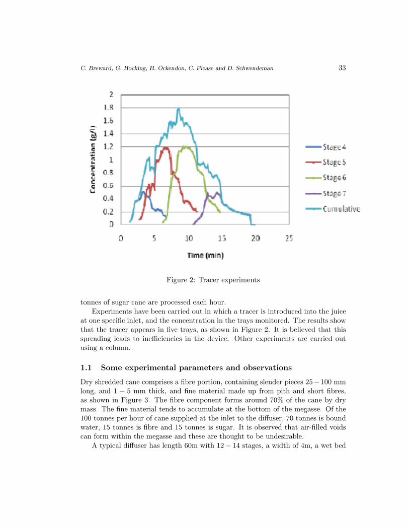
Figure 2: Tracer experiments

tonnes of sugar cane are processed each hour.

Experiments have been carried out in which a tracer is introduced into the juiceat one specific inlet, and the concentration in the trays monitored. The results showthat the tracer appears in five trays, as shown in Figure 2. It is believed that thisspreading leads to inefficiencies in the device. Other experiments are carried outusing a column.

1.1 Some experimental parameters and observations

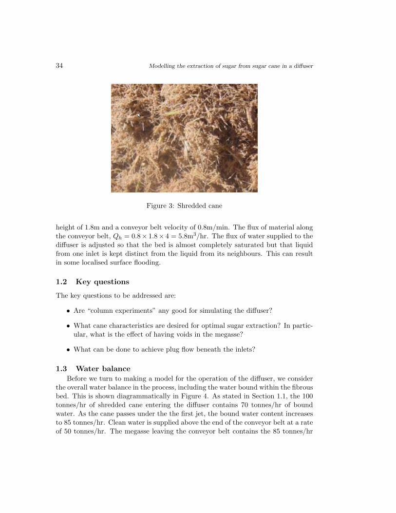
Dry shredded cane comprises a fibre portion, containing slender pieces 25− 100 mmlong, and 1 − 5 mm thick, and fine material made up from pith and short fibres,as shown in Figure 3. The fibre component forms around 70% of the cane by drymass. The fine material tends to accumulate at the bottom of the megasse. Of the100 tonnes per hour of cane supplied at the inlet to the diffuser, 70 tonnes is boundwater, 15 tonnes is fibre and 15 tonnes is sugar. It is observed that air-filled voidscan form within the megasse and these are thought to be undesirable.

A typical diffuser has length 60m with 12− 14 stages, a width of 4m, a wet bed


Figure 3: Shredded cane

height of 1.8m and a conveyor belt velocity of 0.8m/min. The flux of material alongthe conveyor belt, Qh = 0.8× 1.8× 4 = 5.8m3/hr. The flux of water supplied to thediffuser is adjusted so that the bed is almost completely saturated but that liquidfrom one inlet is kept distinct from the liquid from its neighbours. This can resultin some localised surface flooding.

1.2 Key questions

The key questions to be addressed are:

• Are “column experiments” any good for simulating the diffuser?

• What cane characteristics are desired for optimal sugar extraction? In partic-ular, what is the effect of having voids in the megasse?

• What can be done to achieve plug flow beneath the inlets?

1.3 Water balanceBefore we turn to making a model for the operation of the diffuser, we consider

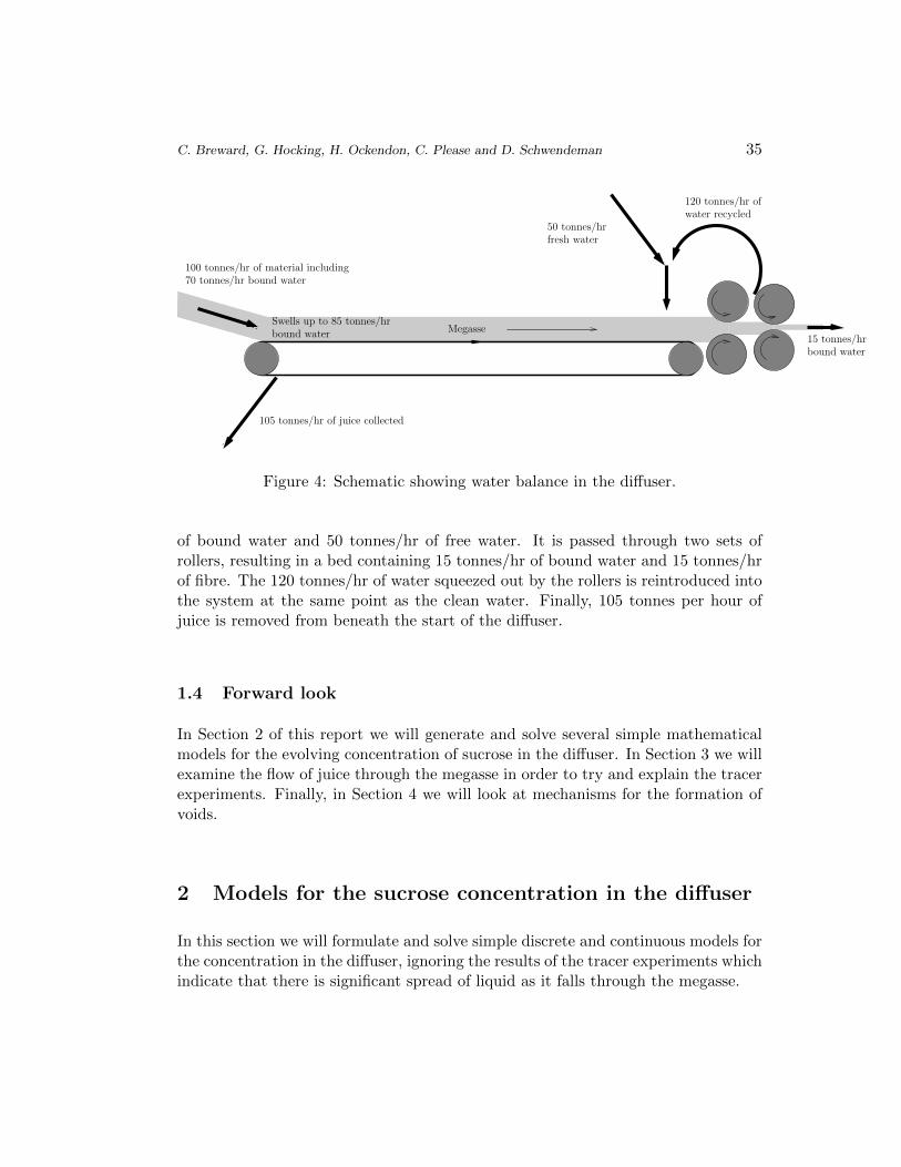
the overall water balance in the process, including the water bound within the fibrousbed. This is shown diagrammatically in Figure 4. As stated in Section 1.1, the 100tonnes/hr of shredded cane entering the diffuser contains 70 tonnes/hr of boundwater. As the cane passes under the the first jet, the bound water content increasesto 85 tonnes/hr. Clean water is supplied above the end of the conveyor belt at a rateof 50 tonnes/hr. The megasse leaving the conveyor belt contains the 85 tonnes/hr


50 tonnes/hrfresh water

105 tonnes/hr of juice collected

120 tonnes/hr ofwater recycled

15 tonnes/hrbound water

Swells up to 85 tonnes/hrbound water

100 tonnes/hr of material including70 tonnes/hr bound water

Megasse

Figure 4: Schematic showing water balance in the diffuser.

of bound water and 50 tonnes/hr of free water. It is passed through two sets ofrollers, resulting in a bed containing 15 tonnes/hr of bound water and 15 tonnes/hrof fibre. The 120 tonnes/hr of water squeezed out by the rollers is reintroduced intothe system at the same point as the clean water. Finally, 105 tonnes per hour ofjuice is removed from beneath the start of the diffuser.

1.4 Forward look

In Section 2 of this report we will generate and solve several simple mathematicalmodels for the evolving concentration of sucrose in the diffuser. In Section 3 we willexamine the flow of juice through the megasse in order to try and explain the tracerexperiments. Finally, in Section 4 we will look at mechanisms for the formation ofvoids.

2 Models for the sucrose concentration in the diffuser

In this section we will formulate and solve simple discrete and continuous models forthe concentration in the diffuser, ignoring the results of the tracer experiments whichindicate that there is significant spread of liquid as it falls through the megasse.


cN ci+1 ci ci−1 c1

c0ci−2cN−1

s0s1sN si+1 si si−1

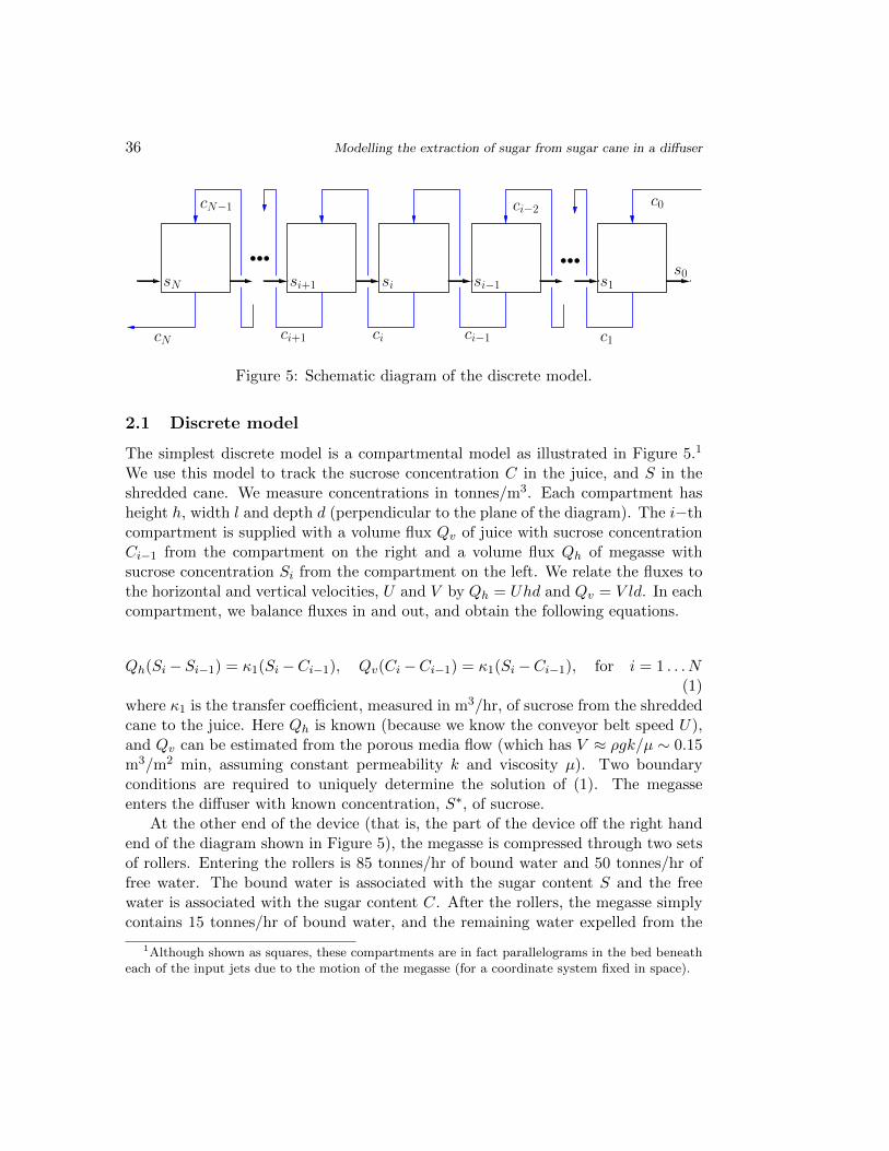
Figure 5: Schematic diagram of the discrete model.

2.1 Discrete model

The simplest discrete model is a compartmental model as illustrated in Figure 5.1

We use this model to track the sucrose concentration C in the juice, and S in theshredded cane. We measure concentrations in tonnes/m3. Each compartment hasheight h, width l and depth d (perpendicular to the plane of the diagram). The i−thcompartment is supplied with a volume flux Qv of juice with sucrose concentrationCi−1 from the compartment on the right and a volume flux Qh of megasse withsucrose concentration Si from the compartment on the left. We relate the fluxes tothe horizontal and vertical velocities, U and V by Qh = Uhd and Qv = V ld. In eachcompartment, we balance fluxes in and out, and obtain the following equations.

Qh(Si − Si−1) = κ1(Si −Ci−1), Qv(Ci −Ci−1) = κ1(Si −Ci−1), for i = 1 . . . N(1)

where κ1 is the transfer coefficient, measured in m3/hr, of sucrose from the shreddedcane to the juice. Here Qh is known (because we know the conveyor belt speed U),and Qv can be estimated from the porous media flow (which has V ≈ ρgk/µ ∼ 0.15m3/m2 min, assuming constant permeability k and viscosity µ). Two boundaryconditions are required to uniquely determine the solution of (1). The megasseenters the diffuser with known concentration, S∗, of sucrose.

At the other end of the device (that is, the part of the device off the right handend of the diagram shown in Figure 5), the megasse is compressed through two setsof rollers. Entering the rollers is 85 tonnes/hr of bound water and 50 tonnes/hr offree water. The bound water is associated with the sugar content S and the freewater is associated with the sugar content C. After the rollers, the megasse simplycontains 15 tonnes/hr of bound water, and the remaining water expelled from the

1Although shown as squares, these compartments are in fact parallelograms in the bed beneatheach of the input jets due to the motion of the megasse (for a coordinate system fixed in space).


megasse is mixed with 50 tonnes/hr of fresh water and reintroduced into the system.We can see that there are several possible boundary conditions that can be imposed:here we give two such possibilities.

If we assume that the sugar in the free water entering the rollers has concentrationC1, then the relationship for C0 reads

C0 =70

170S0 +

50

170C1 = λ1S0 + λ2C1. (2)

However, it is more likely that the sugar in the free water has some combinationof C0 and C1. At the other extreme, if the concentration of sugar in the waterentering the rollers is C0, we have

C0 =70

120S0 = λ3S0. (3)

Clearly the conditions at this end warrant further study. For now, we will assumethat (3) holds. Thus we set

SN = S∗, C0 = λS0. (4)

The solution of (1) and (4) is

CiS∗

=1− Mλ

P − (1− λ)(

1−P1−M

)i1− Mλ

P − (1− λ)MP

(1−P1−M

)N ,SiS∗

=1− Mλ

P −M(1−λ)

P

(1−P1−M

)i1− Mλ

P − (1− λ)MP

(1−P1−M

)N , (5)

where M = κ1/Qh and P = κ1/Qv. We note that the “shape” of the solutionchanges depending on whether M or P is larger. If P > M (and both M and P aresmall), then the solution is of the form

Ci ∼ A1 +B1i−D1i2, (6)

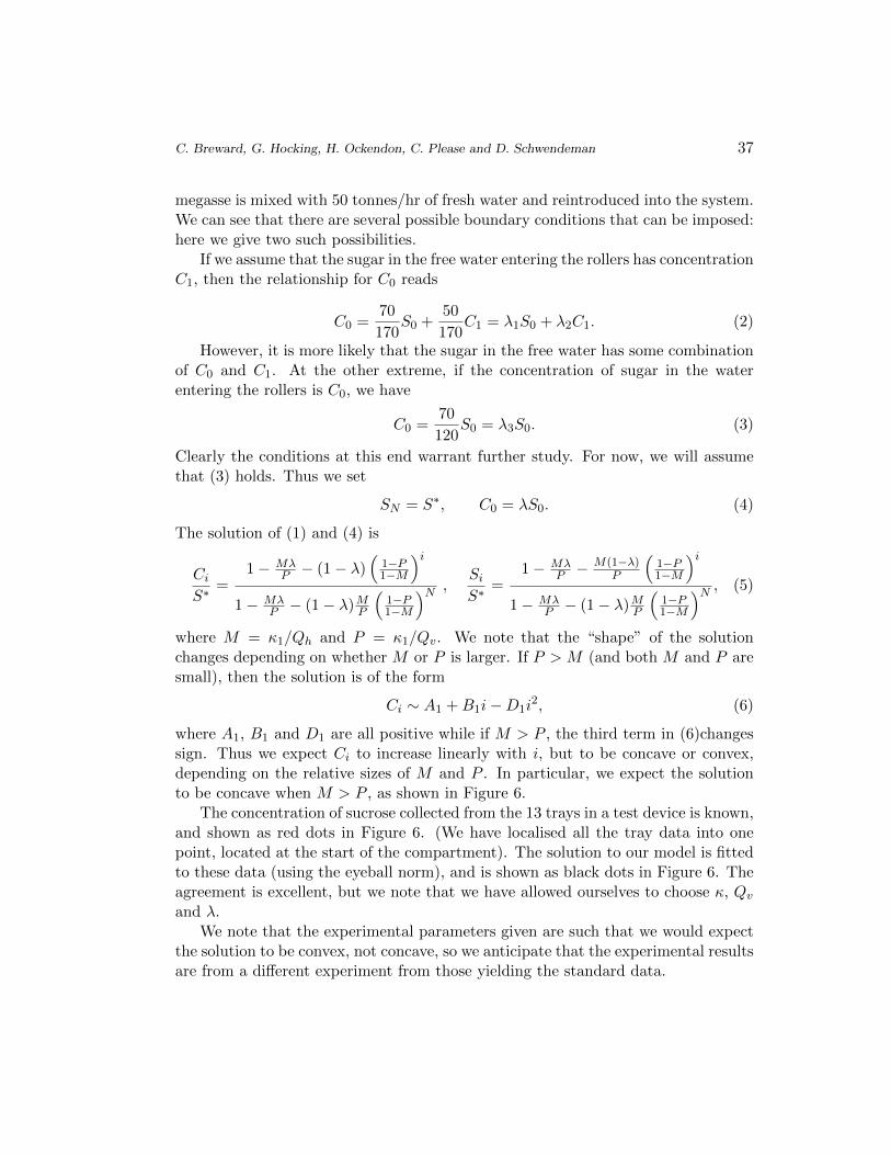
where A1, B1 and D1 are all positive while if M > P , the third term in (6)changessign. Thus we expect Ci to increase linearly with i, but to be concave or convex,depending on the relative sizes of M and P . In particular, we expect the solutionto be concave when M > P , as shown in Figure 6.

The concentration of sucrose collected from the 13 trays in a test device is known,and shown as red dots in Figure 6. (We have localised all the tray data into onepoint, located at the start of the compartment). The solution to our model is fittedto these data (using the eyeball norm), and is shown as black dots in Figure 6. Theagreement is excellent, but we note that we have allowed ourselves to choose κ, Qvand λ.

We note that the experimental parameters given are such that we would expectthe solution to be convex, not concave, so we anticipate that the experimental resultsare from a different experiment from those yielding the standard data.


10 20 30 40 50 60x

2

4

6

8

C

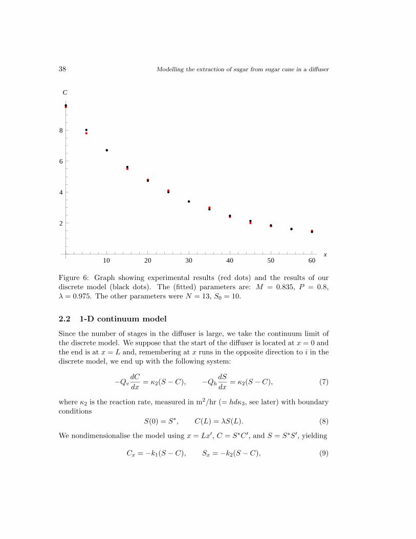
Figure 6: Graph showing experimental results (red dots) and the results of ourdiscrete model (black dots). The (fitted) parameters are: M = 0.835, P = 0.8,λ = 0.975. The other parameters were N = 13, S0 = 10.

2.2 1-D continuum model

Since the number of stages in the diffuser is large, we take the continuum limit ofthe discrete model. We suppose that the start of the diffuser is located at x = 0 andthe end is at x = L and, remembering at x runs in the opposite direction to i in thediscrete model, we end up with the following system:

−QvdC

dx= κ2(S − C), −Qh

dS

dx= κ2(S − C), (7)

where κ2 is the reaction rate, measured in m2/hr (= hdκ3, see later) with boundaryconditions

S(0) = S∗, C(L) = λS(L). (8)

We nondimensionalise the model using x = Lx′, C = S∗C ′, and S = S∗S′, yielding

Cx = −k1(S − C), Sx = −k2(S − C), (9)


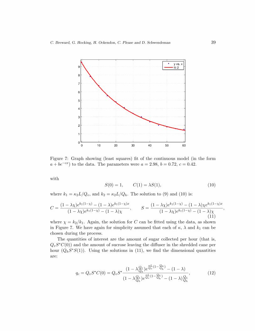
Figure 7: Graph showing (least squares) fit of the continuous model (in the forma+ be−cx) to the data. The parameters were a = 2.98, b = 0.72, c = 0.42.

with

S(0) = 1, C(1) = λS(1), (10)

where k1 = κ2L/Qv, and k2 = κ2L/Qh. The solution to (9) and (10) is:

C =(1− λχ)ek1(1−χ) − (1− λ)ek1(1−χ)x

(1− λχ)ek1(1−χ) − (1− λ)χ, S =

(1− λχ)ek1(1−χ) − (1− λ)χek1(1−χ)x

(1− λχ)ek1(1−χ) − (1− λ)χ,

(11)where χ = k2/k1. Again, the solution for C can be fitted using the data, as shownin Figure 7. We have again for simplicity assumed that each of κ, λ and k1 can bechosen during the process.

The quantities of interest are the amount of sugar collected per hour (that is,QvS

∗C(0)) and the amount of sucrose leaving the diffuser in the shredded cane perhour (QhS

∗S(1)). Using the solutions in (11), we find the dimensional quantitiesare:

qc = QvS∗C(0) = QvS

∗ (1− λQvQh )eκLQv

(1−QvQh

) − (1− λ)

(1− λQvQh )eκLQv

(1−QvQh

) − (1− λ)QvQh

, (12)


5 10 15 20 25

0.5

1.0

1.5

2.0

1 2 3 4 5

0.1

0.2

0.3

0.4

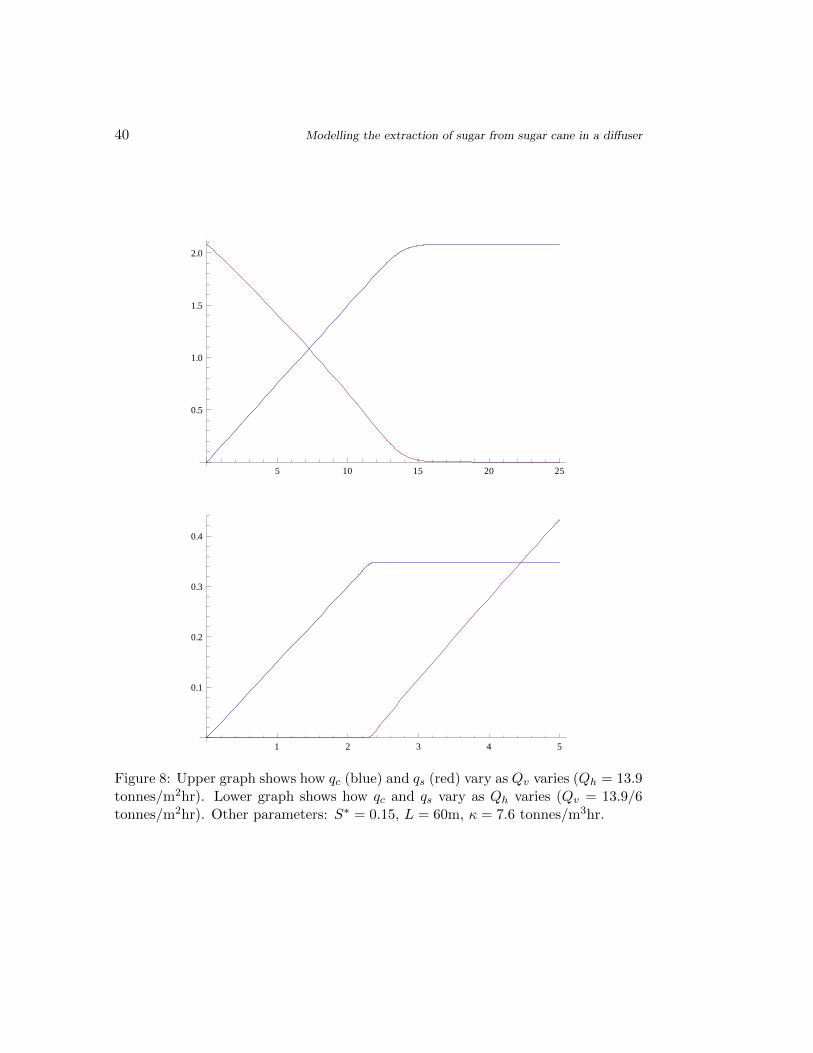
Figure 8: Upper graph shows how qc (blue) and qs (red) vary as Qv varies (Qh = 13.9tonnes/m2hr). Lower graph shows how qc and qs vary as Qh varies (Qv = 13.9/6tonnes/m2hr). Other parameters: S∗ = 0.15, L = 60m, κ = 7.6 tonnes/m3hr.


qs = QhS∗S(1) = QhS

∗ 1− QvQh

(1− λQvQh )− (1− λ)QvQh e− κLQv

(1−QvQh

). (13)

We plot the solutions given in (12) and (13) in Figure 8.We see that (see Figure 8(upper)) that increasing the flux of water through the

system increases the amount of sugar recovered per hour, and decreases the sugarleaving the diffuser still in the megasse, while (see Figure 8(lower)) shows that, abovea certain Qh, the amount of sugar recovered does not change.

2.3 Extension to a 2-D model

In this section we write down the two-dimensional version of the continuous model.We let z be the vertical direction, with z = 0 corresponding to the top surface ofthe megasse. Our 2-D model reads:

USx = −κ3(S − C), UCx + V Cz = κ3(S − C), (14)

where here the reaction rate κ3 has units hr−1. The boundary conditions are

S(0, z) = S∗, (15)

C(x, 0) = λ1

∫ h

0S(L, z)dz + λ2

∫ h

0C(L, z)dz, for x = [L− l, L], (16)

C(x, 0) =1

l

∫ (n+1)l

nlC(x+h

U

V+ l, h)dx for x = [nl, (n+ 1)L], n = 0..n−1. (17)

As an illustration, we take a megasse which is 1 unit high and 30 units long. Plotsof S and C are shown in Figure 9. We see that the concentration of sugar in thejuice increases along the diffuser, and that the concentration of sugar bound in themegasse decreases both with depth through the megasse, and along the megasse.

3 Flow in the porous medium and tracer experiments

We now examine how the juice flows through the megasse from the injection points.We consider a simple model here in the main body of the text and examine a morecomplex and mathematically interesting problem in the Appendix. For the simplemodel we assume that the juice is sprayed at a sufficient rate to ensure that themegasse is saturated and that there is sufficient flooding of the top surface that the


Figure 9: Graphs showing how C and S vary with position x along the diffuser andposition y beneath the surface of the megasse. The parameters used were: λ1 = 0.5,λ2 = 0.5, U = 3, V = 1, κ3 = 0.1, h = 1, L = 30, with 15 collection bins. Herey = z.


resulting flow is one-dimensional. The more complicated problem of determiningthe saturated flow from a finite size source and furthermore finding the flow from afinite source with an unsaturated surrounding region are presented in the Appendix.

For the simple case we shall account for the fact that the megasse may havesome vertical structure and particularly that the permeability may vary with depth.This will allow us to examine possible void behaviour later in the text. Considerthe problem of saturated flow in a region where the permeability varies with depthin the megasse. We assume that the flow is governed by D’Arcy’s law and that thefluid is incompressible. Thus

u = −k(z)

µ∇(p + ρgz), ∇ · u = 0, (18)

where k(z) is the permeability, p is the pressure, ρ is the water density and µ is theviscosity. We are interested in solving this equation across the megasse, which asbefore has thickness h. At the boundaries, we presume that the top (z = h) is keptflooded with a thin layer of juice and that the bottom (z = 0) is simply open, sothat the pressure is atmospheric at both surfaces and hence

p = 0, on z = 0, h. (19)

We note that there is no applied dependence on x and so the governing equationbecomes

kpzz + k′pz + ρgk′ = 0, (20)

which we can integrate to give

kpz + ρgk = constant = µV, (21)

where V can be interpreted as the magnitude of the velocity. We can rearrange (21)and integrate to give

p =

∫ (µV

k(η)− ρg

)dη. (22)

Imposing the two boundary conditions in (19), we then find∫ h

0

µV

k(η)dη = ρgh, (23)

which can be rearranged to give

V =ρgh

µ∫ h0

dηk(η)

=ρg

µ

1

< 1/k >, (24)


where < . > indicates an average value over the depth. We note that the fluidvelocity is constant.

When the tracer is added, the concentration of the tracer, C, will be transportedby convection and diffusion so that, relative to the megasse, C satisfies

Ct − V Cz = D⊥Cxx +D‖Czz. (25)

Here we have assumed that the flow within the porous media gives rise to anisotropicdiffusivity (see Booth [1]). The two diffusivities, in the direction of the flow D‖ andperpendicular to the flow D⊥ can be well represented by

D⊥ =3

16V L, D‖ =

V L

3log

(3V L

2Dm

), (26)

where L is the average pore size (which is around 1mm) and Dm is the diffusivityof the tracer in the juice. This model is valid where V L/Dm, the pore-based Pecletnumber is sufficiently large, as is relevant for transport through the megasse.

We suppose that we inject a bolus of tracer at x = 0 on the top surface at t = 0,that is, we have a point source at x = 0, z = h, and that the transport is governedby (25). We thus have that

C = δ(x), on z = h. (27)

The solution is

C =Q

texp

(− 1

4t

[x2

D⊥+

(z − h+ V t)2

D‖

]), (28)

where Q is determined by considering the size of the bolus.We are interested in determining how the tracer spreads and exits from the

megasse. This can be computed directly from (28), but it is instructive to considerthe case where we can linearise the exponential and gain some insight. We thusapproximate (28) by

C =

{Qt

(1−

(14t

[x2

D⊥+ (z−h+V t)2

D‖

]))when x2

D⊥+ (z−h+V t)2

D‖≤ 4t

0 otherwise.(29)

Hence, at the bottom of the megasse, z = 0, we have

C =

{Qt

(1−

(14t

[x2

D⊥+ (−h+V t)2

D‖

]))when x2

D⊥+ (−h+V t)2

D‖≤ 4t

0 otherwise.(30)

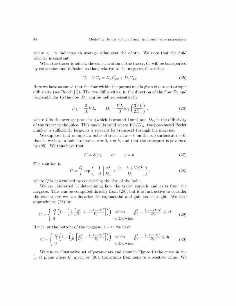
We use an illustrative set of parameters and show in Figure 10 the curve in the(x, t) plane where C, given by (30), transitions from zero to a positive value. We


0 5 10 15 20

0

5

10

15

20

x

t

Figure 10: Plot of ellipse showing region of non-zero C. The parameters are D⊥ = 1,D‖ = 0.01, U = 1, V = 0.1, h = 1.


8 10 12 14 16 18 20t

0.1

0.2

0.3

0.4

C

Figure 11: Average concentration in each bin as a function of time in five bins, eachof width 4. Other parameters are as in Figure 10.


see that the region of nonzero C is enclosed in an ellipse with the minimum in timeto the right of the minimum in space, which is true for an angled ellipse. Crucially,the ellipse is assumed to be much wider than the collector spacing and so we expectthe juice containing the tracer to be collected in more than one box. Further, we seethat, if the spacial separation between the two minima is greater than the collectorspacing, or if the collector junction is between the two minima, then the juice willarrive in the downstream box before the upstream box. We illustrate this behaviourby assuming that the collectors are spaced 4 units apart, and we show the outputof our simulated tracer experiment in Figure 11

Comparing the curves in Figure 11 with those in Figure 2, we see that both therelative sizes and timing of the collection of the juice is reproduced and thus webelieve that our model explains this phenomena.

We note that our parameter choices were made in order to create solutions withthe observed behaviour. We have yet to reconcile these with the physical parametersand, in particular, note that if we use more physically realistic numbers then theaspect ratio of the ellipse (in Figure 10) decreases dramatically and the initial arrivaltime of the juice in the bins travels downstream at a constant rate (unlike Figure 11).

4 Simple model for voids

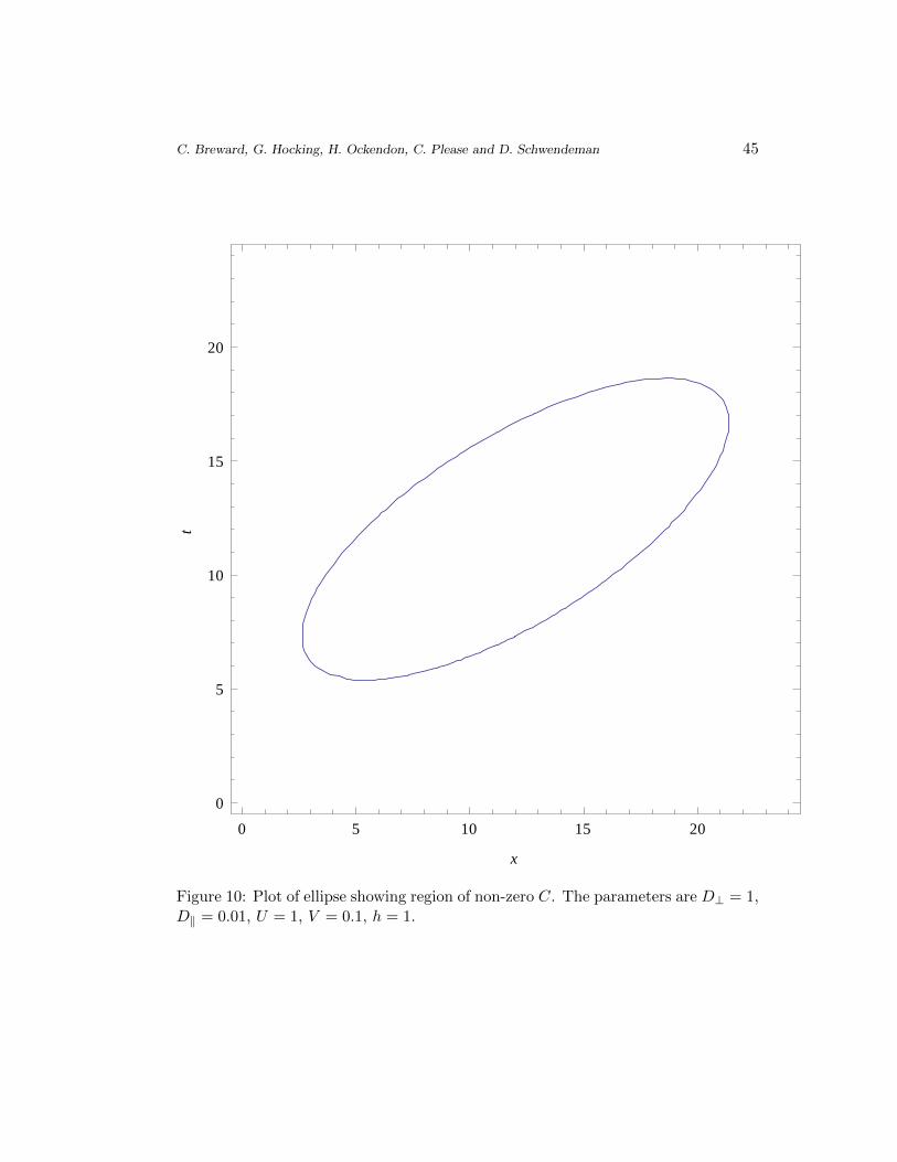
In this section we consider one possible mechanism for the formation and influenceof voids in the megasse which, as noted earlier, are undesirable. These voids areregions of the megasse where it appears that there is little or no water, as illustratedin Figure (12).

The possible mechanism is one of cavitation. To avoid cavitation, we anticipatethat the pressure in the juice must not drop below atmospheric (zero) pressure. We

P = 0

P = 0

u

u

Figure 12: Schematic of a void within the megasse.


expect that, if the megasse has uniform microscopic structure, then the pressureeverywhere is identically atmospheric. Hence, we briefly explore here how the pres-sure depends on nonuniformity within the megasse and identify regions of negativepressure as places where cavitation and hence voids can occur.

These regions where the the pressure is negative (less than atmospheric) are ripefor any stray air bubbles to coalesce, and form a stable cavity. This model does notdescribe other factors such as surface tension and geometric structure, however, itdoes highlight unwanted pressure zones. We will therefore not examine what theflow through the megasse is when cavitation occurs but only indicate when it mightbe observed.

Our starting assumption is again that the flow is one dimensional, and governedby D’Arcy’s law as outlined and solved in Section 3. The flow was found to have avelocity

V =ρgh

µ∫ h0

dηk(η)

(31)

with the pressure being given by

p = ρgh

∫ y0 dηk(η)∫ h

0dηk(η)

− z

h

. (32)

In practice, the fines within the megasse tend to move towards the bottom wherethe megasse is more compressed and hence we expect the permeability to decreaseas we approach y = 0 (the permeability would be monotonically increasing with y).Since the pressure gradient is given by

dp

dz= ρgh

1

k(z)∫ h0

dηk(η)

− 1

h

. (33)

we note that, if k(z) is monotonic increasing, then dp/dz can only be zero at onepoint. Hence we conclude that if the permeability decreases monotonically with itsminimum at the bottom, the pressure is everywhere greater or equal to zero so novoids appear, while the converse occurs if the permeability increases monotonically.

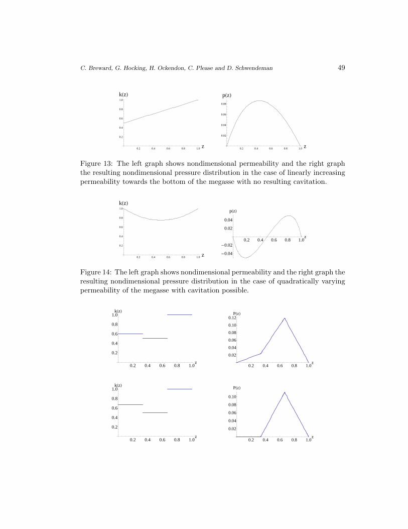
Some numerical experiments were performed with various piecewise constantpermeabilities, and the pressure determined, as shown in Figures 13 and 14. Fromthis we conclude that if there are regions of low permeability above regions of highpermeability, there is the possibility of cavitation. However, the natural tendencyfor the low permeability regions to be at the bottom of the megasse are likely tomitigate against this behaviour. We note that if mechanical devices, such as rotating


0.2 0.4 0.6 0.8 1.0 z

0.2

0.4

0.6

0.8

1.0

kHzL

0.2 0.4 0.6 0.8 1.0 z

0.02

0.04

0.06

0.08

pHzL

Figure 13: The left graph shows nondimensional permeability and the right graphthe resulting nondimensional pressure distribution in the case of linearly increasingpermeability towards the bottom of the megasse with no resulting cavitation.

0.2 0.4 0.6 0.8 1.0 z

0.2

0.4

0.6

0.8

1.0

kHzL

0.2 0.4 0.6 0.8 1.0z

-0.04

-0.02

0.02

0.04

pHzL

Figure 14: The left graph shows nondimensional permeability and the right graph theresulting nondimensional pressure distribution in the case of quadratically varyingpermeability of the megasse with cavitation possible.

0.2 0.4 0.6 0.8 1.0z

0.2

0.4

0.6

0.8

1.0kHzL

0.2 0.4 0.6 0.8 1.0z

0.02

0.04

0.06

0.08

0.10

0.12PHzL

0.2 0.4 0.6 0.8 1.0z

0.2

0.4

0.6

0.8

1.0kHzL

0.2 0.4 0.6 0.8 1.0z

0.02

0.04

0.06

0.08

0.10

PHzL


0.2 0.4 0.6 0.8 1.0z

0.2

0.4

0.6

0.8

1.0kHzL

0.2 0.4 0.6 0.8 1.0z

-0.02

0.02

0.04

0.06

0.08

0.10PHzL

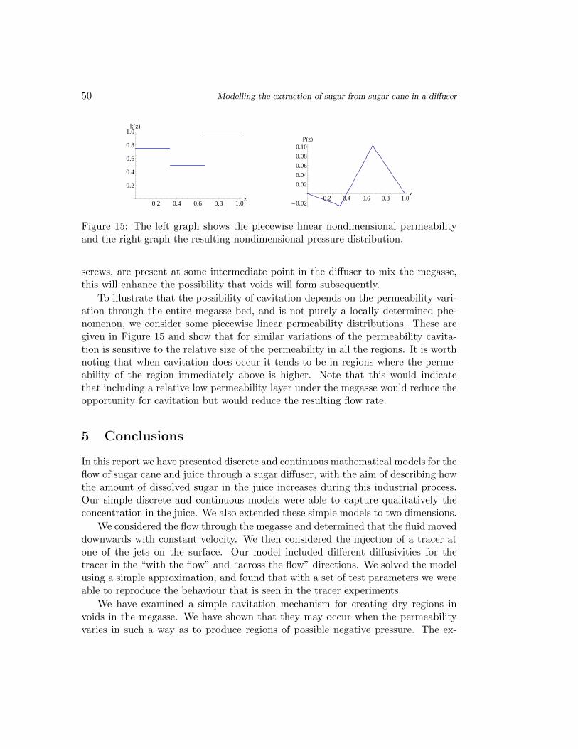
Figure 15: The left graph shows the piecewise linear nondimensional permeabilityand the right graph the resulting nondimensional pressure distribution.

screws, are present at some intermediate point in the diffuser to mix the megasse,this will enhance the possibility that voids will form subsequently.

To illustrate that the possibility of cavitation depends on the permeability vari-ation through the entire megasse bed, and is not purely a locally determined phe-nomenon, we consider some piecewise linear permeability distributions. These aregiven in Figure 15 and show that for similar variations of the permeability cavita-tion is sensitive to the relative size of the permeability in all the regions. It is worthnoting that when cavitation does occur it tends to be in regions where the perme-ability of the region immediately above is higher. Note that this would indicatethat including a relative low permeability layer under the megasse would reduce theopportunity for cavitation but would reduce the resulting flow rate.

5 Conclusions

In this report we have presented discrete and continuous mathematical models for theflow of sugar cane and juice through a sugar diffuser, with the aim of describing howthe amount of dissolved sugar in the juice increases during this industrial process.Our simple discrete and continuous models were able to capture qualitatively theconcentration in the juice. We also extended these simple models to two dimensions.

We considered the flow through the megasse and determined that the fluid moveddownwards with constant velocity. We then considered the injection of a tracer atone of the jets on the surface. Our model included different diffusivities for thetracer in the “with the flow” and “across the flow” directions. We solved the modelusing a simple approximation, and found that with a set of test parameters we wereable to reproduce the behaviour that is seen in the tracer experiments.

We have examined a simple cavitation mechanism for creating dry regions invoids in the megasse. We have shown that they may occur when the permeabilityvaries in such a way as to produce regions of possible negative pressure. The ex-


istence of such regions depends on the permeability variations through the entiredepth of the bed but is exacerbated by regions of low permeability away from thebottom of the bed.

All our models contain parameters which need to be obtained from experiments:the next stage would be to use these to give our models real predictive power.

References

[1] R. Booth, Miscible flow through porous media, DPhil Thesis, Oxford University,2008.

[2] Bear, J. Dynamics of Fluids in Porous Media, McGraw Hill, 1972.

[3] Harr, M. Groundwater and Seepage, McGraw Hill, 1962.

[4] Zhukovsky, N. “Collected Works” Gostekhizdat, Moscow, 1949-1950.

Appendix

Flow through megasse due to applied pressure

In this appendix we consider the problem of porous media flow through the megassein the situation where the top surface has a region of excess pressure. In this case,we consider how water spreads and flows downward through a previously dry sectionof megasse. As a result, there is a region of fully saturated flow surrounded by adry region. In what follows we consider the flow downward from a single source andthen extend this to the case of multiple sources.

A.1 Equations

The flow of a liquid through a porous medium can be studied by defining the piezo-metric head

Φ =p

ρg+ Y, (34)

where Y is elevation, p is the pressure, ρ is density and g is gravitational acceleration.The usual model assumes the flow is dictated by Darcy’s Law, which states that thefluid velocity u is given as

u = −κ∇Φ, (35)

where κ = ρgk/µ, k is permeability of the material and µ is dynamic viscosity ofthe fluid. Combining Darcy’s Law with the continuity equation gives

∇ · u = −κ∇2Φ = 0 (36)


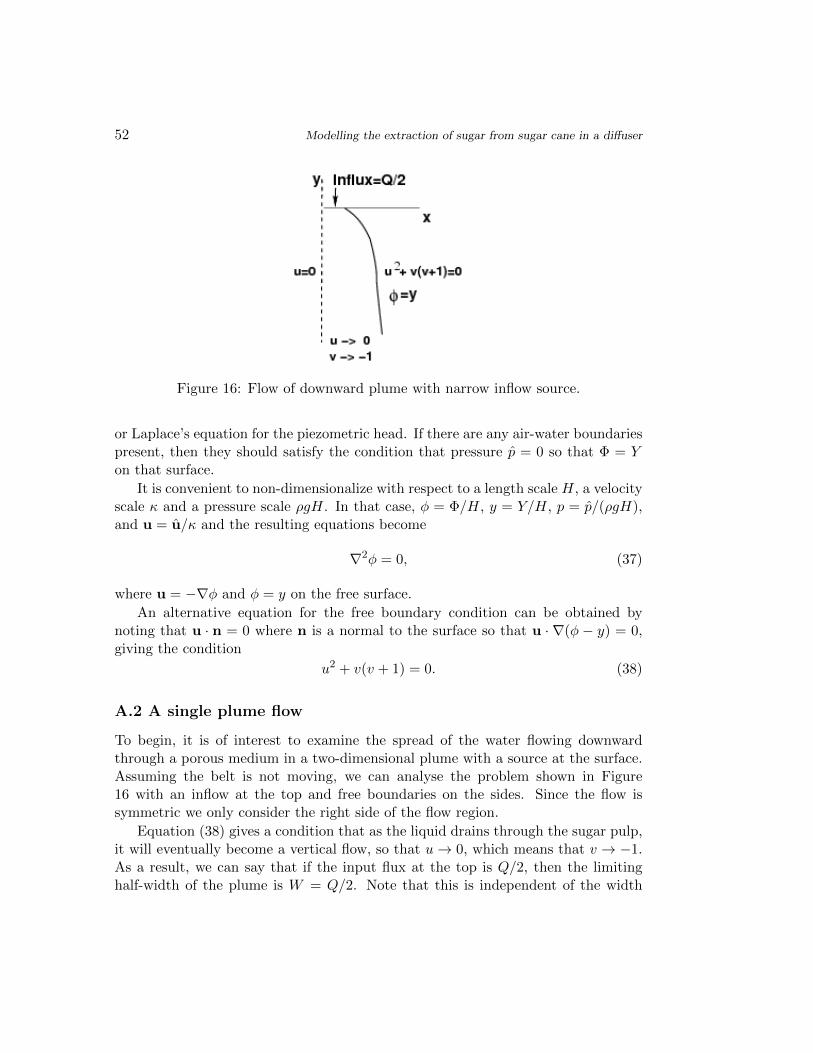
Figure 16: Flow of downward plume with narrow inflow source.

or Laplace’s equation for the piezometric head. If there are any air-water boundariespresent, then they should satisfy the condition that pressure p = 0 so that Φ = Yon that surface.

It is convenient to non-dimensionalize with respect to a length scale H, a velocityscale κ and a pressure scale ρgH. In that case, φ = Φ/H, y = Y/H, p = p/(ρgH),and u = u/κ and the resulting equations become

∇2φ = 0, (37)

where u = −∇φ and φ = y on the free surface.

An alternative equation for the free boundary condition can be obtained bynoting that u · n = 0 where n is a normal to the surface so that u · ∇(φ − y) = 0,giving the condition

u2 + v(v + 1) = 0. (38)

A.2 A single plume flow

To begin, it is of interest to examine the spread of the water flowing downwardthrough a porous medium in a two-dimensional plume with a source at the surface.Assuming the belt is not moving, we can analyse the problem shown in Figure16 with an inflow at the top and free boundaries on the sides. Since the flow issymmetric we only consider the right side of the flow region.

Equation (38) gives a condition that as the liquid drains through the sugar pulp,it will eventually become a vertical flow, so that u→ 0, which means that v → −1.As a result, we can say that if the input flux at the top is Q/2, then the limitinghalf-width of the plume is W = Q/2. Note that this is independent of the width


Figure 17: Solutions for flows with initial flux of Q = 1 and initial plume half-widthsof Q/4, Q/3, Q/2 and Q/2 + 0.1. All surfaces become vertical exponentially.

over which the liquid is drained onto the surface. The question then is how quicklyis this thickness reached?

A neat method to consider this flow is to use the Zhukovsky function, [3, 4] whichis defined as

θ = iz + f = Ae−f/α (39)

where f = φ+iψ is a complex potential, z = x+iy are the coordinates in the physicalplane and α and A are constants to be determined. The velocity components arerelated to the complex potential via the relations u = −φx and v = −φy. Thisfunction is analytic and hence satisfies Laplace’s equation. The method will providea solution for seeping flow from a ditch of some width and depth. The shape of theditch is not known a-priori, but in this problem is not particularly relevant since ourinterest is in the behaviour of the free surface. More detailed explanation of this canbe found in [3].

Taking real and imaginary parts in equation (39) we find that in general

x = −ψ −Ae−φ/α sin ψα , (40)

y = φ−Ae−φ/α cos ψα . (41)

We note that on the line of symmetry x = 0, ψ = 0 and on the free surfaceψ = −Q/2 and also φ = y. Therefore on the surface it must be that either A = 0 or


cosψ/α = 0, that is, ψ/α = (2n + 1)π/2 and so α = −Q/(2n + 1)/π. It turns outthat the appropriate choice of n is n = 0, (for other choices see [3]) in which casewe have α = −Q/π and using y = φ gives

x =Q

2−Aeπy/Q. (42)

As expected, the width of the plume approaches Q/2 as y → −∞. Noting that aty = 0, x = x0, the initial half-width of the inflow region, we obtain A = Q/2 − x0.It is clear from this result that convergence to the final plume thickness occurs veryquickly (exponentially in fact). It is of interest to compute the shape of the drainage“ditch”, although it is only of minor concern and not relevant to our conclusions.On the surface of the ditch, φ = 0, and so we can use equation (40) with φ = 0 over−Q/2 < ψ < 0 to find that

xD = −ψ − (Q/2− x0) sin

(ψπ

−Q

), (43)

yD = (x0 −Q/2) cos

(ψπ

Q

). (44)

Some examples of surface shapes are given in Figure 17. The dashed lines indicatethe shape of the “ditches” for x0 = Q/4 and x0 = Q/3. The case x0 = Q/2 is anexact solution with x = Q/2 everywhere (the inflow region is exactly the same as thefinal plume width) with a flat seepage zone through the top. The case x0 = Q/2+0.1is simply an example to show that even if the inflow region is slightly wider thanthe final plume width, the plume narrows to the limiting thickness. In this case the“ditch” is actually a small mound (not shown).

The main point of this work is to show that for reasonable inflow widths acrossthe top of the sugar pulp the transition to the final plume thickness is exponentiallyfast, meaning we can assume that the flow is close to uniform as it exits from thebottom of the pulp layer. It is also important to note that the limiting dimensionalvelocity through the bottom is given by the magnitude of the hydraulic conductivity,that is, v → −κ.

A.3 Saturated solution

The above work seems to suggest that the flow reaches its full width very quickly(exponentially in fact) and so if the flow is large enough to fill each section betweeninflow points then we can assume the region is fully saturated. It is also reasonableto assume that the flow is periodic in the x-direction (before the horizontal motionis included). The results above suggest that the flux from the base will be close touniform, which will allow us to specify the flow fully in terms of the inflow.


The equations describing a saturated flow of this kind are, similar to above,Laplace’s equation for the piezometric head and periodicity in the x direction. Innon-dimensional coordinates we define y = 0 to be the bottom and y = 1 to be thetop of the layer. On the top surface we can specify the inflow to be a step-function

φy =

0 −L < x < −β/2−V0 −β/2 < x < β/2

0 β/2 < x < L

on y = H

where 2L is the distance between inflow sources and β is the width of the source ofwater. We could specify any inflow function, but this seems to closely approximatethe current situation. We assume the water is injected directly into the surface. Onthe bottom we can specify the flux so that

φy = −VB, on y = 0, −L < x < L , (45)

where V0β = 2VBL by conservation. It is possible to account for some of theseconditions by choosing φ carefully. Using separation of variables we can write

φ(x, y) = −VBy − cx+∞∑k=0

ak coshλky cosλkx (46)

where λk = 2kπ/L. Thus we note that this form satisfies the conditions at y = 0and x = ±L. It remains to satisfy the top surface condition at y = 1, for which wecan invoke orthogonality of the eigenfunctions and obtain,

a0 =V0L− 2βVB

L, (47)

ak =−VBL sinλkβ

(kπ)2 sinhλk, k = 1, 2, 3, ... (48)

In order to see the streamlines of the flow we can use the Cauchy-Reimannequations to find the streamfunction

ψ(x, y) = −cy + VBL

∞∑k=1

sinλkβ

(kπ)2 sinhλksinhλky sinλkx . (49)

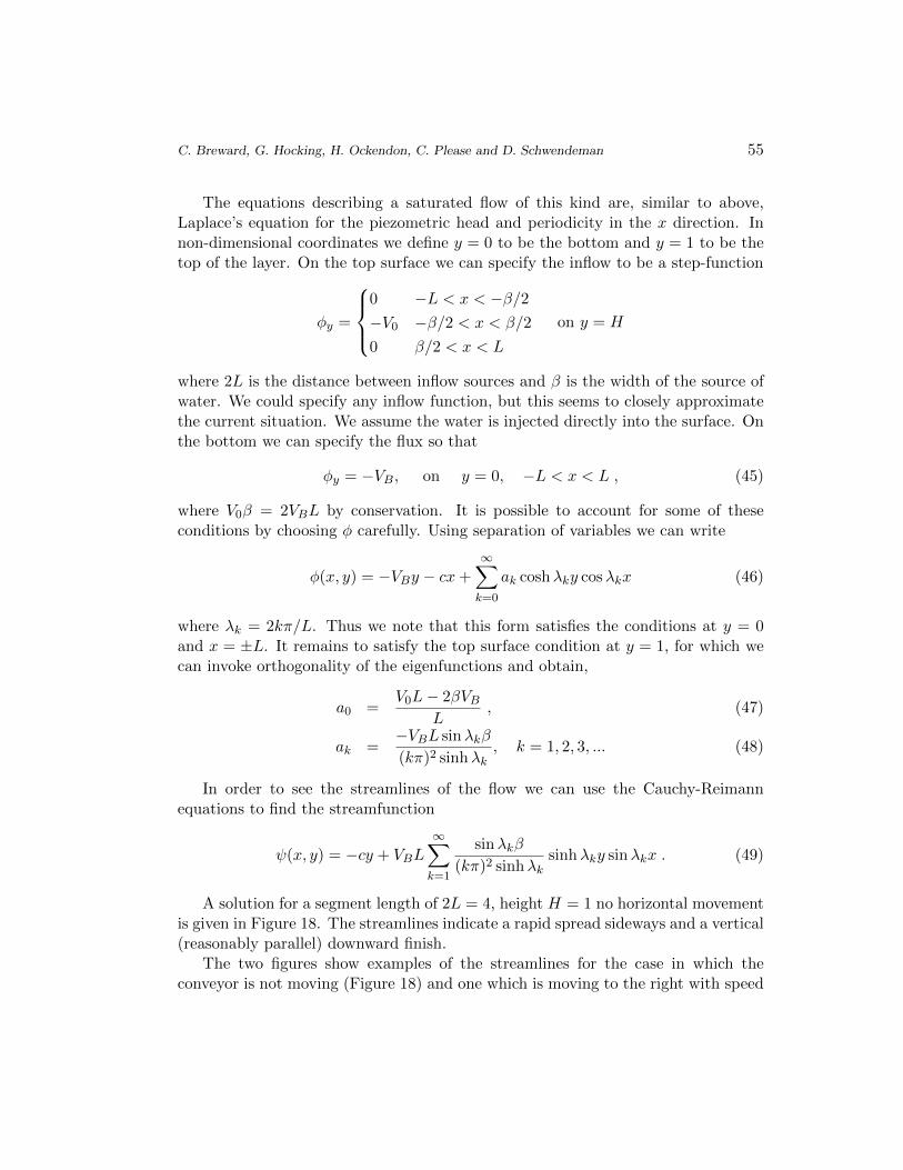
A solution for a segment length of 2L = 4, height H = 1 no horizontal movementis given in Figure 18. The streamlines indicate a rapid spread sideways and a vertical(reasonably parallel) downward finish.

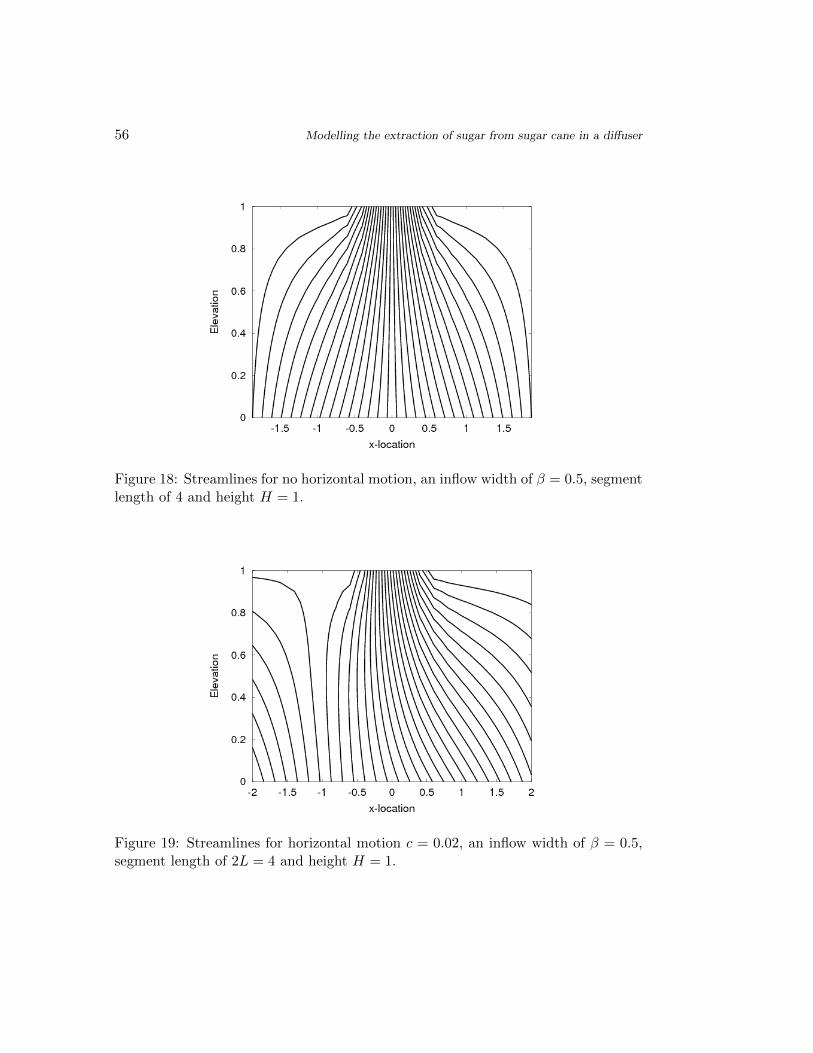
The two figures show examples of the streamlines for the case in which theconveyor is not moving (Figure 18) and one which is moving to the right with speed


Figure 18: Streamlines for no horizontal motion, an inflow width of β = 0.5, segmentlength of 4 and height H = 1.

Figure 19: Streamlines for horizontal motion c = 0.02, an inflow width of β = 0.5,segment length of 2L = 4 and height H = 1.


c = 0.02. The streamlines of these flows are steady, even though the conveyor ismoving the sugar pulp along. The results indicate that there are dividing streamlinesbetween each inflow section and according to this model the fluid from each inflowstays within those bounds. The water from each inflow source will then be moreor less captured in a section of length 2L downstream a distance of approximatelyD = cT = cκ/H from the inflow source, where c is the conveyor speed, 2L is thedistance between inflow points, κ is the hydraulic conductivity and H is the heightof the sugar cane pulp layer.

A.4 Comments

The results above indicate that the water inflow will quickly spread to its final plumethickness and join up with the plume from the next inflow. The flow out through thebottom should then be fairly uniform. Assuming saturated flow, the liquid will passthrough the layer remaining within the horizontal confines of each section (subjectto horizontal translation).

This model does not take account of possible mixing at the dividing streamlinesor the possibility of preferred pathways and nor does it allow for variable permeabilitynear the base of the layer. It would seem likely, however, that these effects may notbe great - altering the timing of the water’s passage through the layer rather thanthe width of the section, since this is fixed by the process. A more complicatedmodel could be invoked to consider this, but in effect an average permeability wouldseem to be adequate to capture the main behaviour.

MODELLING THE EXTRACTION OF SUGAR FROM … Modelling the extraction of sugar from sugar cane in a di...

Documents

Transcript of MODELLING THE EXTRACTION OF SUGAR FROM … Modelling the extraction of sugar from sugar cane in a di...