
Modelling the DGEBA-EDA poly-epoxy reactivity towards ...
185
HAL Id: tel-01988563 https://tel.archives-ouvertes.fr/tel-01988563 Submitted on 21 Jan 2019 HAL is a multi-disciplinary open access archive for the deposit and dissemination of sci- entific research documents, whether they are pub- lished or not. The documents may come from teaching and research institutions in France or abroad, or from public or private research centers. L’archive ouverte pluridisciplinaire HAL, est destinée au dépôt et à la diffusion de documents scientifiques de niveau recherche, publiés ou non, émanant des établissements d’enseignement et de recherche français ou étrangers, des laboratoires publics ou privés. Modelling the DGEBA-EDA poly-epoxy reactivity towards copper experimental and numerical approach Andreas Gavrielides To cite this version: Andreas Gavrielides. Modelling the DGEBA-EDA poly-epoxy reactivity towards copper experimental and numerical approach. Materials. Université Paul Sabatier - Toulouse III, 2017. English. NNT: 2017TOU30300. tel-01988563
Transcript of Modelling the DGEBA-EDA poly-epoxy reactivity towards ...
HAL Id: tel-01988563https://tel.archives-ouvertes.fr/tel-01988563
Submitted on 21 Jan 2019
HAL is a multi-disciplinary open accessarchive for the deposit and dissemination of sci-entific research documents, whether they are pub-lished or not. The documents may come fromteaching and research institutions in France orabroad, or from public or private research centers.
L’archive ouverte pluridisciplinaire HAL, estdestinée au dépôt et à la diffusion de documentsscientifiques de niveau recherche, publiés ou non,émanant des établissements d’enseignement et derecherche français ou étrangers, des laboratoirespublics ou privés.
Modelling the DGEBA-EDA poly-epoxy reactivitytowards copper experimental and numerical approach
Andreas Gavrielides
To cite this version:Andreas Gavrielides. Modelling the DGEBA-EDA poly-epoxy reactivity towards copper experimentaland numerical approach. Materials. Université Paul Sabatier - Toulouse III, 2017. English. �NNT :2017TOU30300�. �tel-01988563�
et discipline ou spécialité
Jury :
le
Université Toulouse 3 Paul Sabatier (UT3 Paul Sabatier)
Andreas GAVRIELIDES
mardi 28 novembre 2017
Modélisation du poly-époxy DGEBA-EDA et de sa réactivité vis à vis du cuivre:
approche expérimentale et numérique
Modelling the DGEBA-EDA poly-epoxy and its reactivity towards copper:
experimental and numerical approach
ED SDM : Sciences et génie des matériaux - CO034
CIRIMAT UMR CNRS 5085
Dominique COSTA, Directrice de Recherche, Chimie ParisTech, Paris, Rapporteur
Tzonka MINEVA, Directrice de Recherche, Institut Charles Gerhardt, Montpellier, Rapporteur
Patrice RAYNAUD, Directeur de Recherche, LAPLACE, Toulouse, Examinateur
Frederic MERCIER, Chargé de Recherche, Université Grenoble Alpes, Examinateur
Corinne LACAZE-DUFAURE, Professeur, CIRIMAT, Toulouse, Directrice de thèse
Thomas DUGUET, Chargé de Recherche, CIRIMAT, Toulouse, Co-directeur de thèse
Yohann LEDRU, Ingénieur Docteur, MECANO-ID, Toulouse, Invité
Pr. Corinne LACAZE-DUFAURE
Dr. Thomas DUGUET


Acknowledgements
I would like to start by expressing my sincere gratitude to my supervisors Professor Corinne
Lacaze-Dufaure and Dr. Thomas Duguet who trusted me with these project and gave me the
opportunity to work with them. They are both great scientific minds and excellent characters
and truly passionate about anything they are involved and the advancement of science. They
were always there for me and without our valuable discussions and their dedication to the
success of this project, this thesis would not have been feasible. The knowledge they have
instilled in me will stay forever and I am grateful for the supplies they have provided for the
open road that lies ahead of me. They have not only provided the knowledge but also the skills
necessary to achieve my dreams. I will cherish our moments and hope in the future that our
roads will once again converge.
I would like to thank Professor Paul S. Bagus for his enormous help with the Hartree-Fock
ΔSCF calculations which are a part of this thesis and for providing us with some very interesting
results on the calculation of XPS spectra.
Professor Doros Theodorou and PhD student Mr. Orestis Ziogos had a big impact on this project
as our discussions both in Athens (National Technical University of Athens) as well as
following discussions after returning back to France helped us accelerate the calculations on
the Molecular Dynamics front.
To both Professor Theodorou and Professor Andreas Boudouvis, I would like to say a big thank
you for directing me in the path of executing a PhD thus giving me three of my best years.
I would also like to thank the members of the SURF team of which I was a proud member
during my 3-year PhD course and would like to extend special thanks to Dr. Maëlenn Aufray
for our very helpful discussions and Mr. Jérôme Esvan for his valuable help in the experimental
XPS spectra acquisition as well as the mounting of the metal evaporator on the UHV chamber.
I am also lucky to have met and discussed with Dr. Constantin Vahlas in numerous occasions.
Through our discussions I managed to change my character in a way I am sure will help me for
years to come.

My PhD thesis could not have been executed if not for my two wonderful parents Kleanthis and
Marina which were there for me from the beginning and continue to support me until this very
day. I owe them everything and they have shaped me throughout the years. My two brothers
Pavlos and Alexandros were also there when I needed them and I am sure they will grow to be
excellent.
To my grandparents Pavlos, Virginia, Andreas and Alexandra I need to express my gratitude
which cannot be contained in words as they are pillars of my life and have been there in all of
my moments even from a distance. They have sacrificed a lot for me and this PhD is dedicated
to their memory.
Finally I would like to thank all of my friends that were right beside me, from my childhood
years, to the 5 wonderful years in Athens and the 3 amazing years in France. They have stood
by me in every moment, both good and bad and without them there would be no point in
anything.
This PhD thesis is finally dedicated to everyone who is not afraid to pursue their dreams no
matter how impossible they may seem. I want you to know that if you put your mind on anything
you can do it and even if you fail, persist and you can only win. Things will come around even
in unpredictable ways.
As far as the financial support of this thesis is concerned I would like to thank the French
Ministère de l’Enseignement supérieur et de la Recherche for providing the funds for the
execution of this thesis.

vii
Table of Contents
Introduction générale ............................................................................................................................ 1
Chapter 1: Objectives and methods ..................................................................................................... 5
1.1 Introduction ....................................................................................................................................... 5
1.2 Why poly-epoxy polymers and what is the benefit of their surface metallization? .......................... 5
1.3 Calculations on polymers: ................................................................................................................. 8
1.3.1 Quantum calculations ................................................................................................................. 9
1.3.1.1 The Schrödinger’s equation ................................................................................................. 9
1.3.1.2 The Born-Oppenheimer approximation ............................................................................ 10
1.3.1.3 The Hartree-Fock method.................................................................................................. 12
1.3.1.4 Density functional theory (DFT) calculations ................................................................... 13
1.3.2 Classical Calculations ............................................................................................................... 21
1.3.2.1 Molecular Mechanics (MM) basics ................................................................................... 21
1.3.2.1 The molecular Dynamics (MD) method ............................................................................ 26
1.4 Computational Facilities.................................................................................................................. 31
1.5 Conclusion ....................................................................................................................................... 32
Chapter 2: Experimental formation of model poly-epoxy surfaces and characterizations .......... 37
2.1 Introduction ..................................................................................................................................... 37
2.2 Pristine (non-metallized) poly-epoxy surface ................................................................................. 38
2.2.1 Synthesis protocol of a pristine low-roughness poly-epoxy surface ........................................ 38
2.2.2. Characterizations ..................................................................................................................... 39
2.2.2.1 Bulk Characterizations ...................................................................................................... 39
2.2.2.2 Surface Characterizations .................................................................................................. 47
2.3 Metallized poly-epoxy surface ........................................................................................................ 56
2.3.1 Protocol for metallizing a poly-epoxy surface in ambient temperature with Cu ...................... 56
2.3.2 AFM results .............................................................................................................................. 58
2.3.3 XPS results ............................................................................................................................... 59
2.4 Conclusion ....................................................................................................................................... 60
Chapter 3: HF and DFT computations for the simulation of XPS spectra .................................... 63
3.1 Introduction ..................................................................................................................................... 63
3.2 General introduction to XPS ........................................................................................................... 63
3.3 Calculation of XPS spectra .............................................................................................................. 65
3.3.1 Hartree-Fock calculations ......................................................................................................... 65

viii
3.3.2 Density Functional Theory calculations ................................................................................... 67
3.4 Poly-epoxy pristine polymer surface ............................................................................................... 68
3.4.1 Geometry Optimization Calculations ....................................................................................... 68
3.4.2 XPS calculations using Hartree-Fock theory ........................................................................... 70
3.4.3 XPS calculations using DFT theory ......................................................................................... 76
3.4.3.1 Simulation of the XPS spectrum for the pristine polymer ................................................. 77
3.4 Polymer metallized with Cu ............................................................................................................ 80
3.4.1 Adsorption of Cu atom on the dimer model ............................................................................. 80
3.4.2 Simulation of the XPS spectrum of the metallized polymer .................................................... 83
3.5 Calculation of the charges on the atoms for the DM simulations ................................................... 86
3.6 Conclusion ....................................................................................................................................... 88
Chapter 4: Molecular Dynamics Simulations ................................................................................... 93
4.1 Introduction ................................................................................................................................. 93
4.2 Simulation of bulk polymer properties ........................................................................................ 93
4.3 Description of the methodology and cross-linking algorithm ..................................................... 96
4.4 Results ....................................................................................................................................... 101
4.4.1 MD simulations on pure monomers: validation of the GAFF force field .......................... 101
4.4.1.1 MD calculations on DGEBA ....................................................................................... 101
4.4.1.2 MD calculations on EDA ............................................................................................ 103
4.4.2. MD calculations on the 2DGEBA:1EDA liquid mixture .................................................. 105
4.4.3 Polymerization of the 2DGEBA:1EDA system ................................................................. 109
4.4.4 Glass transition temperature of the model polymer ............................................................ 111
4.5 Conclusion ................................................................................................................................. 113
Conclusions générales et perspectives ............................................................................................. 117
Annexes .............................................................................................................................................. 121
Annex A: Generalized Amber Force Field (GAFF) parameters and atom types ................................ 123
Annex B: The velocity Verlet algorithm ............................................................................................ 134
Annex C: Structure comparison of DGEBA, EDA and dimer molecules optimized using different
computational conditions .................................................................................................................... 135
Annex D: Comparison between RESP and AM1-BCC methodologies for partial charge calculations of
the EDA, DGEBA, dimer and trimer molecules ................................................................................. 137
Annex E: Step-by-Step Guide to execute a simulation box generation using the PACKMOL code . 146
Annex F: Cross-linking code .............................................................................................................. 150
Annex G: LAMMPS MD scripts description ..................................................................................... 151

ix
Annex H: DGEBA simulation boxes and NPT simulation results for different initial parameters .... 159
Annex I: EDA simulation boxes and NPT simulation results for different initial parameters ........... 161
Annex J: Test of several temperatures for NPT simulations of the DGEBA, EDA and stoichiometric
mixture simulation boxes .................................................................................................................... 163


Introduction générale
1
Introduction générale
Les composites à matrice polymère sont de plus en plus utilisés en tant que matériaux de
structure, et en tant que substituts pour des composants métalliques, notamment dans le
domaine aéronautique et spatial1. Ils réduisent le poids des assemblages et abaissent la
consommation de carburant des avions ou des lanceurs spatiaux. Ils étaient jusqu’alors
seulement utilisés pour des pièces « secondaires » comme certains morceaux de carlingue ;
mais la gamme d'application s’est maintenant largement étendue à des composants
fonctionnels, tels que les revêtements d'aile et de fuselage, le train d'atterrissage, ou encore les
réservoirs de réfrigérant de satellite.
La mise en forme des pièces composites est relativement avantageuse. Ces dernières peuvent
adopter des formes complexes qui, pour des pièces métalliques, nécessiteraient de l'usinage et
de l’assemblage, par exemple. De plus, leur utilisation réduit le nombre de fixations et de joints
– qui sont des points de défaillance potentielle - que ce soit pour les aéronefs ou pour les
satellites. Les matériaux composites permettent donc d’abaisser les coûts, en réduisant le
nombre de composants, et en procédant à des conceptions uni-pièce chaque fois que cela est
possible.
Cependant, le remplacement des pièces métalliques par des polymères nécessite souvent une
fonctionnalisation de surface afin de retrouver des propriétés optiques, électriques,
magnétiques, biomédicales, esthétiques ou chimiques2. Le principal inconvénient quand il s'agit
de recouvrir ou de greffer la surface des composites à base de polymère provient de l'énergie
de surface très faible de ces derniers. Il en résulte une mouillabilité et des forces d’adhésion
faible lorsque du métal y est déposé. Les efforts consentis jusqu’à présent pour pallier ce
phénomène reposent exclusivement sur des études empiriques. Nous pensons que le manque de
simulations et de modèles est un obstacle à un développement technologique efficace. Le
développement d'un modèle précis pour la surface des polymères peut aider à la conception de
surfaces sur mesure avec un bon contrôle sur la réactivité chimique, et donc sur les processus
de fonctionnalisation subséquents. La portée de ce travail n’est donc pas limitée à la seule
métallisation des composites.
Nous choisissons de réaliser une étude à la fois expérimentale et théorique de la surface d’un
polymère époxy et de sa métallisation en lien avec des projets applicatifs en cours dans notre

Modelling the DGEBA-EDA poly-epoxy and its reactivity towards copper: experimental and
numerical approach
2
groupe de recherche (Surfaces : Réactivité et Protection, du CIRIMAT, Toulouse). L’objectif
principal est de développer un modèle de surface qui soit utilisable comme template pour
l’étude de mécanismes élémentaires, tels que l’adsorption/désorption, la
germination/croissance, ou le greffage chimique.
Les simulations numériques sont l’outil choisi afin d’obtenir des informations sur la surface, et
sur les mécanismes d’adsorption et de germination-croissance des films métalliques. L'échelle
de temps que l'on veut simuler, la taille du système étudié et les propriétés qui doivent être
calculées conduisent au choix de deux méthodologies spécifiques. D’une part, nous réalisons
des calculs statiques (qui ne tiennent pas compte de l'évolution du système avec le temps) dans
le cadre de la théorie de la fonctionnelle de la densité (DFT)3. L’échelle concerne ici des
phénomènes quantiques et des systèmes de dimensions de l’ordre de quelques nanomètres. La
DFT est utilisée pour déterminer avec précision les paramètres structurels et les propriétés
électroniques de molécules et de solides modèles. Nous cherchons alors à simuler les spectres
XPS du polymère poly-époxyde à l'aide d'un dimère modèle formé d'une molécule de
diglycidylether de biphénol A (DGEBA) connectée à une molécule d'éthylène diamine (EDA).
Cette petite molécule permet de prendre en compte toutes les liaisons possibles du polymère
réticulé réel, mais en conservant un faible nombre d'atomes (61 atomes) pour faciliter les
calculs. En utilisant deux méthodes de calcul (Hartree-Fock4,5, ΔSCF6, DFT et uGTS8–10), nous
tentons d’améliorer les connaissances générales à propos de cette surface et de sa réactivité.
D’autre part, nous effectuons des calculs qui tiennent compte de l'évolution temporelle du
système dans le cadre de la dynamique moléculaire (MD) classique. Ces simulations
numériques concernent des systèmes plus grands (jusqu'à l'échelle micrométrique) et pour
différentes échelles de temps (jusqu'à quelques ns)11,12. Ils permettent de déterminer des
propriétés structurales (distribution de distances interatomiques intra- et inter- moléculaire, par
ex.), physico-chimiques (température de transition vitreuse, ...), ou encore mécaniques (Module
d’Young, ...) de grands ensemble de particules ou de molécules. Ici, nous utilisons la dynamique
moléculaire avec trois objectifs: (i) équilibrer et calculer les propriétés physiques et structurales
des liquides (DGEBA et EDA) réactifs purs et de leur mélange, (ii) simuler le processus de
polymérisation13,14 qui crée le réseau poly-époxyde à partir du mélange liquide de nos
monomères, et (iii) obtenir les propriétés du polymère.

Introduction générale
3
Pour la partie expérimentale, nous avons développé un protocole de synthèse d’une surface
poly-époxyde de faible rugosité (Ra < 1 nm), homogène et présentant peu de défauts. Une telle
surface « modèle » est souhaitée car il faut être en mesure d'observer les nano-îlots et les
clusters métalliques clairement, sans qu’ils soient confondus avec les aspérités de surface, et
que la germination ne doit pas être exclusivement hétérogènes (sur les défauts) ; auxquels cas
les modèles simples sur lesquels reposent les calculs seraient faux. Les caractérisations
volumiques du polymère (taux de polymérisation et température de transition vitreuse) sont
conduites par FTIR et DSC. La surface non métallisée est caractérisée par AFM et XPS et est
ensuite métallisée à température ambiante par évaporation sous ultravide. Cette technique
permet une adsorption sans énergie cinétique et correspond donc mieux aux calculs quantiques
d’adsorption. La surface métallisée est aussi caractérisée par AFM et XPS afin de déterminer
la réactivité du polymère vis-à-vis du métal, la formation des liaisons interfaciales du métal
avec le polymère, et observer la croissance des films de Cu.
Ce manuscrit de thèse est organisé de la manière suivante. Dans le chapitre 1, nous allons
détailler les théories sur lesquelles reposent les calculs quantiques et classiques, et comment ils
nous aiderons dans le développement d’un modèle de surface. Dans le chapitre 2, nous
montrerons le protocole expérimental choisi pour la formation des surfaces de poly-époxydes
modèles, ainsi que les caractérisations volumique et de surface, avant et après métallisation.
Dans le chapitre 3, nous allons détailler les différentes méthodes qui peuvent être utilisées pour
simuler les spectres XPS de la surface vierge et métallisée grâce à l'utilisation d'une molécule
dimère modèle. Enfin, dans le chapitre 4, nous démonterons les capacités de la dynamique
moléculaire dans la simulation des propriétés physiques et structurales des liquides purs
(réactifs) et de leur mélange. Enfin, nous montrerons comment, avec l'utilisation d’un code
multi-étapes développé pendant la thèse, nous créons un polymère modèle, dont les propriétés
physiques et structurelles sont comparables aux résultats de la bibliographie.
Bibliographie
1. Aerospace materials — past, present, and future. Aerospace Manufacturing and Design Available
at: http://www.aerospacemanufacturinganddesign.com/article/amd0814-materials-aerospace-
manufacturing/. (Accessed: 25th September 2017)
2. E. Sacher (ed.). Metallization of Polymers 2. (Plenum Publishers, 2002).
3. Hohenberg, P. & Kohn, W. Inhomogeneous Electron Gas. Phys. Rev. 136, B864–B871 (1964).
4. Bagus, P. S., Ilton, E. S. & Nelin, C. J. The interpretation of XPS spectra: Insights into materials
properties. Surf. Sci. Rep. 68, 273–304 (2013).
5. Bagus, P. S., Freeman, A. J. & Sasaki, F. Prediction of New Multiplet Structure in Photoemission
Experiments. Phys. Rev. Lett. 30, 850–853 (1973).

Modelling the DGEBA-EDA poly-epoxy and its reactivity towards copper: experimental and
numerical approach
4
6. Ziegler, T., Rauk, A. & Baerends, E. J. On the calculation of multiplet energies by the hartree-
fock-slater method. Theor. Chim. Acta 43, 261–271 (1977).
7. Janak, J. F. Proof that θΕ/θni=εi in density-functional theory. Phys. Rev. B 18, 7165–7168 (1978).
8. Endo, K., Kaneda, Y., Okada, H., Chong, D. P. & Duffy, P. Analysis of X-ray Photoelectron
Spectra of Eight Polymers by deMon Density-Functional Calculations Using the Model
Oligomers. J. Phys. Chem. 100, 19455–19460 (1996).
9. Motozaki, W., Otsuka, T., Endo, K. & Chong, D. P. Electron Binding Energies of Si 2p and S 2p
for Si- and S-containing Substances by DFT Calculations Using the Model Molecules. Polym. J.
36, 600–606 (2004).
10. Otsuka, T., Endo, K., Suhara, M. & Chong, D. P. Theoretical X-ray photoelectron spectra of
polymers by deMon DFT calculations using the model dimers. J. Mol. Struct. 522, 47–60 (2000).
11. Alder, B. J. & Wainwright, T. E. Studies in Molecular Dynamics. I. General Method. J. Chem.
Phys. 31, 459–466 (1959).
12. Andersen, H. C. Molecular dynamics simulations at constant pressure and/or temperature. J.
Chem. Phys. 72, 2384–2393 (1980).
13. Jang, C., Sirk, T. W., Andzelm, J. W. & Abrams, C. F. Comparison of Crosslinking Algorithms in
Molecular Dynamics Simulation of Thermosetting Polymers. Macromol. Theory Simul. 24, 260–
270 (2015).
14. Sirk, T. W. et al. High strain rate mechanical properties of a cross-linked epoxy across the glass
transition. Polymer 54, 7048–7057 (2013).

Chapter 1. Objectives and Methods
5
Chapter 1: Objectives and methods
1.1 Introduction
In this chapter, our objective is to describe in details the aims of the project and to give some
insight into the methods used for the computational studies which are further analyzed in
Chapters 3 and 4. We present elements of quantum and classical methods, together with the
computational tools. Concerning the experimental work, methods and technics are included
together with the state of the art in Chapter 2.
1.2 Why poly-epoxy polymers and what is the benefit of their surface metallization?
Poly-epoxy polymers are widely implemented in three families of applications: adhesives,
paints, and composite materials1 . The latter, such as epoxy/C fibers composites, is increasingly
found in a wealth of devices and parts in the fields of leisure (skis, rackets, boats, golf clubs,
etc.), or transports, aeronautics and space (cars, aircrafts, satellites, etc.), to name but a few.
These composite materials possess stiffness and Young’s modulus that compare well with
metallic alloys but with a much lower chemical reactivity and density. Therefore, they allow
mass reduction and a large increase of parts durability. Replacement of metallic parts by
polymers often requires surface functionalization in order to acquire optical, electrical,
magnetic, biomedical, aesthetic, or chemical properties. The main drawback of the coating or
grafting of the surface of polymer-based composites comes from the very low surface energy
of such materials once polymerized. This leads to a poor wettability rendering painting or gluing
difficult, and resulting in poor adhesion. The surface energy of poly-ether ether ketone (PEEK)
or poly-epoxy is approximately 40-50 mJ/m2 to be compared to approximately 500 mJ/m2 for
aluminum. Moreover, the polar component (due to H bonding) is as low as 6-7 mJ/m2 which
inhibits the use of simple functionalization protocols2–4. Hence, the reactivity of poly-epoxy
surfaces is of major concern regarding functionalization pretreatments and/or treatments. The
lack of simulations and models is an obstacle to an efficient technology development which
nowadays relies on empirical studies, exclusively. Therefore, the development of an accurate
model for the surface of poly-epoxies can help in the design of tailored surfaces with a good
control on chemical reactivity, and therefore on subsequent metallization processes. Until now
very few attempts have been made5–8, whereas this family of materials is strategic in many

Modelling the DGEBA-EDA poly-epoxy and its reactivity towards copper: experimental and
numerical approach
6
industrial sectors. A metallization model should include a polymer surface model, which could
be used to study adsorption/desorption of metallic atoms, the nucleation and growth of the
metallic coating.
The early stages of polymer metallization are far from thermodynamic equilibrium conditions
since isolated metals atoms are adsorbed on the polymer surface. After deposition the metal
atoms may diffuse on the surface or into the polymer. Metal atoms encountering each other
form clusters at the surface and in the polymer bulk. These clusters are stable if their size
exceeds the size of a critical radius (a minimum number of atoms). At higher coverages metal
atoms increasingly form a thin film with a more or less 3-dimensional aspect.9 This is true when
nucleation is homogeneous and not driven by defects/traps. Actually, there are two possibilities:
preferential nucleation where metal atoms are trapped at preferred sites or defects, and
homogeneous nucleation where nuclei are formed by metal atoms random encounters. Both
processes have been observed in polymer metallization and they usually rely upon the specific
reactivity of the metal towards the polymer surface10. Two opposite examples are given below
with Al and Cu.
The adsorption energy of Cu on polyimide, 0.6±0.1 eV is surprisingly high. The activation
energy for surface diffusion is lower (e.g. 0.2±0.05 eV).9 Cu will thus diffuse to long distances
before nucleation. This absence of chemical reactivity with polyimide is supported by
experiments where Cu migrates inside the polyimide films to form copper agglomerates that
are nearly spherical in shape.11 Davis et al.12 assumed that copper does not react with polyimide
at low coverages but that there is a change in bond order of the polyimide carbonyl groups
induced by the copper at higher coverages. Bond order is the number of bonding pairs of
electrons between two atoms. In the case of a covalent bond between two atoms, a single bond
has a bond order of one, a double bond a bond order of two and so on. They found, however,
no evidence for copper in an oxidized state. It is correct that Cu is not very reactive towards the
polyimide surface, and largely less reactive than Al. However, other studies have shown the
preferential adsorption of Cu on hydroxyls of the polyimide surface13–16, counter arguing Davis
et. al. hypothesis. The story is different with Al that interacts strongly with the polyimide
surface, the C=O group being the preferential site for metal bonding.17 Another illustration of
the higher reactivity of Al with polymers is found in fundamental studies of the Al/
Poly(ethylene terephthalate) interfacial bonding. PET is widely used for packaging.

Chapter 1. Objectives and Methods
7
Unfortunately its diffusion barrier properties are insufficient and an aluminum metallization
layer is required. A theoretical study18 (supported by previous experiments19 has been
performed by calculating atomic orbitals for monomers in interactions with an Al atom. In the
XPS core level data, the C1s component corresponding to the C=O group is strongly affected
by Al adsorption, with a large modification of the electronic charge distribution on that site. Al
atoms are also found to bind covalently to the phenyl rings; however the corresponding
complexes are significantly less stable than those involving Al–ester bonding. Overall, the first
step of deposition of Al on PET proceeds by the saturation of the C=O sites, followed by an
increasing number of Al-Al interactions which favor the formation of dense Al layers. It is
unclear whether Al does adsorb on phenyls or not, because once C=O have been attacked,
phenyls electronic density is strongly modified, to the detriment of Al/phenyl bonding.
Finally, the adhesion of the metallization layer to the polymer substrate is strongly affected by
the above-mentioned mechanisms of adsorption, nucleation and growth. Various theories or
mechanisms of adhesion exist but those responsible for metal-polymer adhesion are mechanical
locking or interlocking, chemical and electrostatic interactions. Whereas the majority of the
thesis work concerns chemical bonding, we introduce these mechanisms briefly.
Mechanical locking or interlocking. In this mechanism the roughness of the substrate
provides a mechanical locking if the deposited film covers the whole surface uniformly.
Additionally, a larger surface area is available for bonding. It becomes
counterproductive if there is no intimate contact between the film and the substrate, with
uncoated areas and voids weakening the polymer/metal interface. In the case of
electroless deposition20, polymer surfaces are etched before, so as to create an extensive
network of fine shallow “holes” on the surface and/or to create deep channels that
connect with each other inside the polymer surface layer. These “holes” and channels
provide attachment points for the electroless metal.
Chemical. According to this theory, bonds are actually formed between the polymer and
the metal. The presence of such chemical bonds should provide a high force of adhesion
and be resistant to moisture and/or ambient ageing or mechanical stress. In case of
electroless deposition of metals on polymers there are many examples where this
specific mechanism of adhesion has been suggested.17,21,22 Examples of Cu and Al
covalent bonding presented above, illustrate this theory.

Modelling the DGEBA-EDA poly-epoxy and its reactivity towards copper: experimental and
numerical approach
8
Electrostatic. This theory support the fact that if two dissimilar materials come in
contact, then a charge transfer takes place and a double layer is thus formed. The two
layers created can be compared to a capacitor and work is consumed in the separation
of these two layers. Derjaguin et al.23, who are the main developers of this theory have
given strong arguments in its favor based on their work of removing a polymer film
from metal surfaces. Skinner et al.24 have also contributed in proving the value of
electrostatic contribution to adhesive performance. Specifically their calculations show
that only if charge densities approach 1021𝑒𝑙𝑒𝑐𝑡𝑜𝑛𝑠/𝑐𝑚3, then electrostatic
interactions will have an important contribution to adhesion.
Chapter 1 is organized as follows. First, we discuss why calculations are performed on polymers
with examples from the bibliography. Then we proceed to describe basic concepts involved in
quantum calculations, and we finish with elements of classical calculations and what settings
we choose for these calculations.
1.3 Calculations on polymers:
Computer simulations can be chosen rather than experiment with the real system for several
reasons: (i) the system we want to study does not exist yet (ii) experiments for the system is
expensive or too time consuming (or too dangerous…) (iii) all the necessary information for
the understanding of a process is not available from experiments. Our project falls in this latter
case. The time scale one wants to simulate, the size of the system studied and the properties
that need to be calculated lead to the choice of a specific methodology. Additionally,
simulations can model both static and dynamic situations. Static calculations refer to
calculations that do not take into account the evolution of the system with time. For instance,
quantum calculations such as standard density functional theory (DFT), can be performed for
systems up to a few nanometers, and can be used to accurately determine structural parameters
and electronic properties of molecules and solids. And if there is no need to get electronic
properties from the computations, static molecular mechanics simulations can be done for larger
systems up to hundreds of nanometers.
Dynamic calculations refer to calculations that take into account the time evolution of the
system. Numerical simulations such as Monte-Carlo (MC) calculations and Molecular
Dynamics (MD), can be performed in the framework of quantum methods or classical

Chapter 1. Objectives and Methods
9
mechanics and can thus be used for larger systems (up to the μm scale) and for various time
scales (up to ns). The choice between MC and MD is dictated by the phenomenon in study.
In the literature, classical molecular simulations, and particularly atomistic ones track the
evolution of model systems for times up to a few tens of ns25 . It thus allows to extract dynamic
properties of polymers. But it used to be (and it is already) problematic since it requires very
long simulations and thus stability of the integrator algorithms for very long times. To overcome
this problem for polymeric systems, several approaches have been proposed over the last
decades. First, parallelization techniques and computer sciences made possible the use of a large
number of processors26 for the calculations. Moreover, for large time scales, new algorithms
involving a multiple time step approach27 were developed for the integration of equations of
motion. They allowed to simulate longer times than the conventional algorithms. But these
technical solutions showed limitations and alternative models of the systems had to be
developed. One consists in the abandon of chemical details of all-atom models and their
substitution by coarse-grained models28,29. These models are simplified representations of the
molecules. “Pseudo-atoms” replace the group of atoms. Much longer simulation times can be
studied than with atomistic models leading to many more realistic network architectures. But
to study properties that depend on the detailed chemical structure, a reverse mapping back to
the original atomistic description is needed.
In our case, we want to develop a model of a poly-epoxy polymer and its metallization. We
need to get information at the atomic level on the electronic structure of the polymer. But we
also need to know how the polymer chains move at different temperatures and times. Using a
combination of quantum calculations (Hartree-Fock and DFT methods for the results presented
in Chapter 3), and classical simulations (atomistic classical Molecular Dynamics in Chapter 4),
we will demonstrate our ability to simulate systems of various sizes and to calculate various
properties (XPS spectra, polymer density…).
1.3.1 Quantum calculations
In this section we present some concepts of quantum chemistry.
1.3.1.1 The Schrödinger’s equation
The Schrödinger’s equation is the basis of any non-relativistic quantum calculations. It
essentially describes the changes over time of a system taking into account quantum effects.
This equation although written for changes over time, also includes a formulation that does not
Modelling the DGEBA-EDA poly-epoxy and its reactivity towards copper: experimental and
numerical approach
10
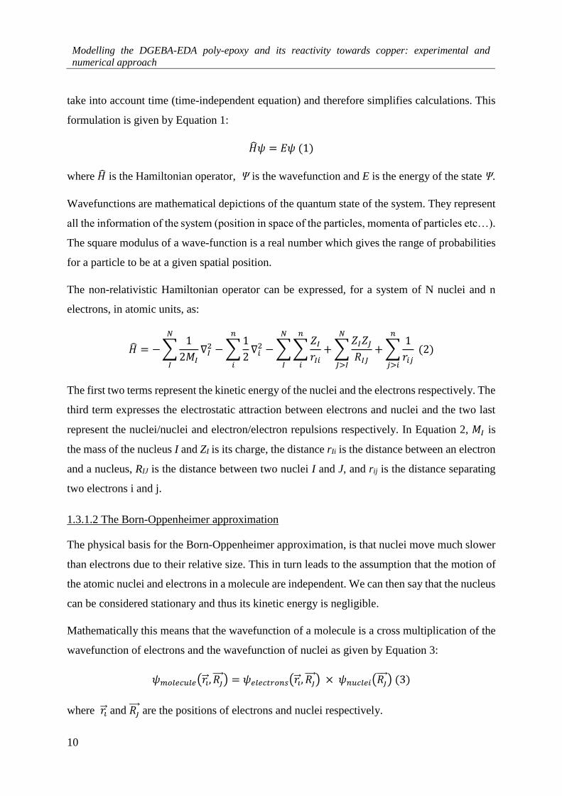
take into account time (time-independent equation) and therefore simplifies calculations. This
formulation is given by Equation 1:
��𝜓 = 𝐸𝜓 (1)
where �� is the Hamiltonian operator, Ψ is the wavefunction and E is the energy of the state Ψ.
Wavefunctions are mathematical depictions of the quantum state of the system. They represent
all the information of the system (position in space of the particles, momenta of particles etc…).
The square modulus of a wave-function is a real number which gives the range of probabilities
for a particle to be at a given spatial position.
The non-relativistic Hamiltonian operator can be expressed, for a system of N nuclei and n
electrons, in atomic units, as:
�� = −∑1
2𝑀𝐼∇𝐼
2
𝑁
𝐼
− ∑1
2∇𝑖
2
𝑛
𝑖
− ∑∑𝑍𝐼
𝑟𝐼𝑖
𝑛
𝑖
𝑁
𝐼
+ ∑𝑍𝐼𝑍𝐽
𝑅𝐼𝐽
𝑁
𝐽>𝐼
+ ∑1
𝑟𝑖𝑗
𝑛
𝑗>𝑖
(2)
The first two terms represent the kinetic energy of the nuclei and the electrons respectively. The
third term expresses the electrostatic attraction between electrons and nuclei and the two last
represent the nuclei/nuclei and electron/electron repulsions respectively. In Equation 2, 𝑀𝐼 is
the mass of the nucleus I and ZI is its charge, the distance rIi is the distance between an electron
and a nucleus, RIJ is the distance between two nuclei I and J, and rij is the distance separating
two electrons i and j.
1.3.1.2 The Born-Oppenheimer approximation
The physical basis for the Born-Oppenheimer approximation, is that nuclei move much slower
than electrons due to their relative size. This in turn leads to the assumption that the motion of
the atomic nuclei and electrons in a molecule are independent. We can then say that the nucleus
can be considered stationary and thus its kinetic energy is negligible.
Mathematically this means that the wavefunction of a molecule is a cross multiplication of the
wavefunction of electrons and the wavefunction of nuclei as given by Equation 3:
𝜓𝑚𝑜𝑙𝑒𝑐𝑢𝑙𝑒(𝑟𝑖 , 𝑅𝑗 ) = 𝜓𝑒𝑙𝑒𝑐𝑡𝑟𝑜𝑛𝑠(𝑟𝑖 , 𝑅𝑗
) × 𝜓𝑛𝑢𝑐𝑙𝑒𝑖(𝑅𝑗 ) (3)
where 𝑟𝑖 and 𝑅𝑗 are the positions of electrons and nuclei respectively.
Chapter 1. Objectives and Methods
11
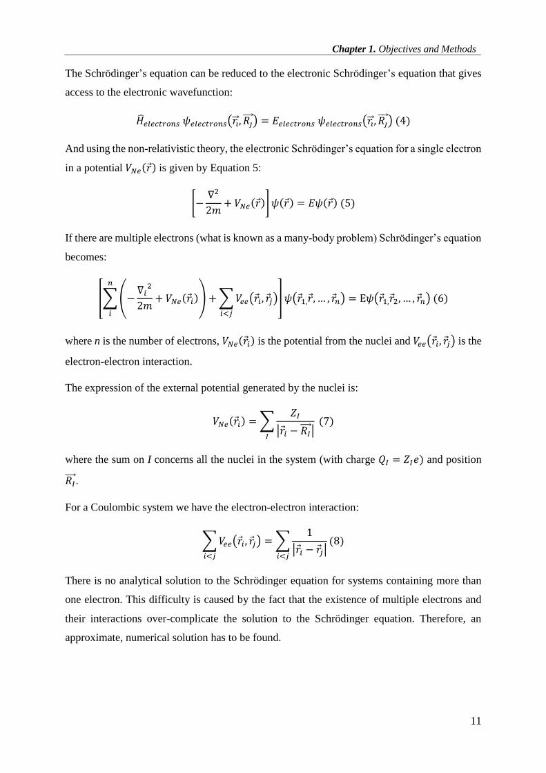
The Schrödinger’s equation can be reduced to the electronic Schrödinger’s equation that gives
access to the electronic wavefunction:
��𝑒𝑙𝑒𝑐𝑡𝑟𝑜𝑛𝑠 𝜓𝑒𝑙𝑒𝑐𝑡𝑟𝑜𝑛𝑠(𝑟𝑖 , 𝑅𝑗 ) = 𝐸𝑒𝑙𝑒𝑐𝑡𝑟𝑜𝑛𝑠 𝜓𝑒𝑙𝑒𝑐𝑡𝑟𝑜𝑛𝑠(𝑟𝑖 , 𝑅𝑗
) (4)
And using the non-relativistic theory, the electronic Schrödinger’s equation for a single electron
in a potential 𝑉𝑁𝑒(𝑟 ) is given by Equation 5:
[−∇2
2𝑚+ 𝑉𝑁𝑒(𝑟 )]𝜓(𝑟 ) = 𝐸𝜓(𝑟 ) (5)
If there are multiple electrons (what is known as a many-body problem) Schrödinger’s equation
becomes:
[∑(−∇𝑖
2
2𝑚+ 𝑉𝑁𝑒(𝑟 𝑖)) + ∑𝑉𝑒𝑒(𝑟 𝑖, 𝑟 𝑗)
𝑖<𝑗
𝑛
𝑖
]𝜓(𝑟 1,𝑟 , … , 𝑟 𝑛) = Ε𝜓(𝑟 1,𝑟 2, … , 𝑟 𝑛) (6)
where n is the number of electrons, 𝑉𝑁𝑒(𝑟 𝑖) is the potential from the nuclei and 𝑉𝑒𝑒(𝑟 𝑖, 𝑟 𝑗) is the
electron-electron interaction.
The expression of the external potential generated by the nuclei is:
𝑉𝑁𝑒(𝑟 𝑖) = ∑𝑍𝐼
|𝑟 𝑖 − 𝑅𝐼 |
𝐼
(7)
where the sum on I concerns all the nuclei in the system (with charge 𝑄𝐼 = 𝑍𝐼𝑒) and position
𝑅𝐼 .
For a Coulombic system we have the electron-electron interaction:
∑𝑉𝑒𝑒(𝑟 𝑖, 𝑟 𝑗)
𝑖<𝑗
= ∑1
|𝑟 𝑖 − 𝑟 𝑗|𝑖<𝑗
(8)
There is no analytical solution to the Schrödinger equation for systems containing more than
one electron. This difficulty is caused by the fact that the existence of multiple electrons and
their interactions over-complicate the solution to the Schrödinger equation. Therefore, an
approximate, numerical solution has to be found.

Modelling the DGEBA-EDA poly-epoxy and its reactivity towards copper: experimental and
numerical approach
12
1.3.1.3 The Hartree-Fock method
Slater introduced a general method to solve Schrödinger’s equation. It was based on the
independent works of Heisenberg and Dirac that proposed that the sign of a wavefunction
changes and becomes the opposite if two electrons are exchanged. Let’s consider the exchange
of two electrons. The Hamiltonian operator is not modified by exchanging their coordinates:
��(𝑟1 , 𝑟2 ) = ��(𝑟2 , 𝑟1 ) (9)
By substituting in Equation 1 we have
��(𝑟𝑖 , 𝑟�� )𝜓(𝑟�� , 𝑟𝑖 ) = 𝐸𝜓(𝑟�� , 𝑟𝑖 ) (10)
We can replace the positions of two electrons with the exchange operator 𝑃𝑖�� and this operator
can exchange positions with the Hamiltonian operator without changing the result (they are
commutative). This leads to Equation 11:
��(𝑟𝑖 , 𝑟�� ) 𝑃𝑖��𝜓(𝑟�� , 𝑟𝑖 ) = 𝑃𝑖����(𝑟𝑖 , 𝑟�� ) 𝜓(𝑟�� , 𝑟𝑖 ) (11)
Which transforms into
[��, 𝑃𝑖��]𝜓 = (��𝑃𝑖�� − 𝑃𝑖����)𝜓 = 0 (12)
Showing that the Hamiltonian and the exchange operator have similar eigenstates. The positions
of two electrons are reverted by two exchanges leading to the value of 𝑃𝑖��2= 1. This means
that the eigenvalues of 𝑃𝑖�� are ±1. Thus there are two wavefunctions corresponding to the
exchange operator. The first for +1 being:
𝜓(𝑆)(𝑟𝑖 , 𝑟�� ) =1
√2[𝜓(𝑟𝑖 , 𝑟�� ) + 𝜓(𝑟�� , 𝑟𝑖 )] (13)
and the antisymmetric for the -1 eigenvalue
𝜓(𝐴)(𝑟𝑖 , 𝑟�� ) =1
√2[𝜓(𝑟𝑖,𝑗 ) − 𝜓(𝑟�� , 𝑟𝑖 )] (14)
where the 1
√2 is the normalization constant. If we consider the Hartree wavefunction which is
essentially the Hamiltonian operator expressed as the product of different electronic
wavefunctions:

Chapter 1. Objectives and Methods
13
𝜓(𝑟𝑖 , 𝑟�� ) = 𝜙𝑖(𝑟 𝑖)𝜙𝑗(𝑟 𝑗) (15)
where 𝜙𝑖 is the one-electron wavefunction, we obtain Equation 16 and 17 that represent the
symmetric and antisymmetric functions:
𝜓(𝑆)(𝑟𝑖 , 𝑟�� ) =1
√2[𝜙𝑖(𝑟 𝑖)𝜙𝑗(𝑟 𝑗) + 𝜙𝑖(𝑟 𝑗)𝜙𝑗(𝑟 𝑖)] (16)
𝜓(𝑆)(𝑟𝑖 , 𝑟�� ) =1
√2[𝜙𝑖(𝑟 𝑖)𝜙𝑗(𝑟 𝑗) − 𝜙𝑖(𝑟 𝑗)𝜙𝑗(𝑟 𝑖)] (17)
From these wavefunctions, only the antisymmetric one is in accordance with Pauli’s exclusion
principle. This is due to the fact that for the case the same electron occupies the same orbital
the wavefunction must be 0, that is 𝑟1 = 𝑟2 . This leads to the conclusion that electronic motions
have antisymmetric functions. The antisymmetric wavefunction of Equation 17 can be written
as a determinant in the following manner:
𝜓(𝑟1 , 𝑟2 ) =1
√2|𝜙1(𝑟 1) 𝜙1(𝑟 2)
𝜙2(𝑟 1) 𝜙2(𝑟 2)| (18)
To respect these rules, at the simplest level, the wave function can be represented by a single
Slater determinant, an antisymmetrized product of one-electron wave functions for n electrons
as presented in Equation 19:
𝜓(𝑟1 , 𝑟2 , … , 𝑟𝑛 ) =1
√𝑛![𝜙1(𝑟 1) ⋯ 𝜙1(𝑟 𝑛)
⋮ ⋱ ⋮𝜙𝑛(𝑟 1) ⋯ 𝜙𝑛(𝑟 𝑛)
] (19)
Using this formulation for the wavefunction, the Hartree-Fock method allows to solve the
Schrödinger equation with a variational method and a set of n-coupled monoelectronic
equations. The Hartree-Fock approach defines a term of Coulomb interaction between an
electron and the mean electron distribution (mean Hartree potential). But the exchange potential
that contributes to the energy does not take into account the correlation effects between the
movements of electrons.

Modelling the DGEBA-EDA poly-epoxy and its reactivity towards copper: experimental and
numerical approach
14
1.3.1.4 Density functional theory (DFT) calculations
The electronic density, 𝜌(𝑟 ), represents the number of electrons per unit volume at a position
in space, 𝑟 . In the framework of the density functional theory, the n-electron wavefunction
Ψ(𝑟1, 𝑟2, 𝑟3, … , 𝑟𝑛) is replaced by the electronic density. Hohenberg and Kohn (HK)30
established two theorems which constitute the foundation of DFT.
First HK theorem (a.k.a The existence theorem)30
This theorem states that all the properties of a system in a ground electronic state are
determined by the ground state electron density 𝜌0(𝑥, 𝑦, 𝑧). This means that if 𝜌0(𝑥, 𝑦, 𝑧)
is known, one can calculate any ground state property.
The theorem generalizes the calculation of any ground state property of a system as a
functional of the ground state electron density function, for example the energy can be
mathematically calculated by
𝐸0 = 𝐹[𝜌0] = 𝐸[𝜌0] (20)
Mathematically speaking the term “functional” describes a function whose argument is
itself a function. Some quantities are simultaneously functionals and functions.
Second HK theorem (a.k.a The variational theorem)30
This theorem states that any trial electron density function will give an energy higher than
(or equal to, if the true electron density function is calculated), the true ground state
energy. So the electronic density of the ground state can be calculated using a variational
method. Although the original Hohenberg-Kohn theorems were proved for non-
degenerate ground states they have been proved to work for degenerate ground states too.

Chapter 1. Objectives and Methods
15
The Kohn-Sham approach
The basic ideas behind the Kohn-Sham31 approach are:
(1) To express the energy as a sum of terms with only one, a relatively small term, that is
the unknown to the equation functional.
(2) To use an initial guess of the electron density ρ in the Kohn-Sham (KS) equations to
calculate an initial guess of the KS orbitals and energy levels.
(3) To use this initial guess to iteratively refine these orbitals and energy levels, in a
manner similar to that used in the HF-SCF method. At every iteration the KS orbitals are
used to calculate an electron density and the energy.
The way to deal with this issue is to separate the electronic energy of our molecule into a
portion which can be calculated accurately, and a relatively small term which requires the
functional.
The electronic energy of a real system is the sum of the electron kinetic energies, the
nucleus-electron attraction potential energies, and the electron-electron interaction
energies as shown in Equation 21:
𝐸[𝜌] = 𝑇[𝜌] + 𝐸𝑁𝑒[𝜌] + 𝐸𝑒𝑒[𝜌] (21)
The nucleus-electron potential energy, 𝐸𝑁𝑒[𝜌] is the sum over all n electrons of the
potential corresponding to attraction of an electron for all the nuclei I:
𝐸𝑁𝑒 [𝜌] = ∫ 𝜌(𝑟 ). 𝑣𝑁𝑒(𝑟 )𝑑𝑟 (22)
𝑤𝑖𝑡ℎ 𝑣𝑁𝑒 = ∑∑−𝑍𝐼
𝑟 𝑖𝐼
𝑁
𝐼=1
𝑛
𝑖=1
(23)
𝑍𝐼
𝑟 𝑖𝐼 is the potential energy due to the interaction of electron i with nucleus I at a given
distance 𝑟 𝑖𝐼
This leads to Equation 24:
𝐸 = 𝑇[𝜌] + ∫𝜌(𝑟 ) 𝑣𝑁𝑒(𝑟 ) 𝑑𝑟 + 𝐸𝑒𝑒[𝜌] (24)
Modelling the DGEBA-EDA poly-epoxy and its reactivity towards copper: experimental and
numerical approach
16
The middle term is a classical electrostatic attraction potential energy expression. A
problem that arises is that there is no way to know the functionals for the kinetic and
potential energies for the other two terms, 𝑇[𝜌] and 𝐸𝑒𝑒[𝜌], making the equation
unsolvable.
Kohn and Sham thus assumed a reference system of non-interacting electrons which gives
the same ground state electron density distribution as the real system (𝜌𝑟𝑒𝑓 = 𝜌0). The
difference in “behavior” between the reference system and the real system can be
accounted into a term that we call “the exchange and correlation functional”.
This non-interacting system has a kinetic energy 𝑇[𝜌]𝑟𝑒𝑓. First in respect to the electronic
kinetic energy, the quantity 𝛥𝑇[𝜌] is defined: 𝛥𝑇[𝜌] ≡ 𝑇[𝜌]𝑟𝑒𝑎𝑙 − 𝑇[𝜌]𝑟𝑒𝑓.
Next, for the electronic potential energy calculation, the term 𝛥𝑉𝐸𝑒𝑒 is defined as the
deviation of the real electron-electron repulsion energy from a classical charge-cloud
coulomb repulsion energy. The classical electrostatic repulsion is calculated from pairs
of infinitesimal densities 𝜌(𝑟 1)𝑑𝑟 1 and 𝜌(𝑟 2)𝑑𝑟 2 (in a classical, non-quantum cloud of
negative charge) separated by a distance 𝑟 12(multiplied by ½ so that the repulsion energy
is not counted twice). It leads to Equation 25:
𝛥𝐸𝑒𝑒[𝜌] = 𝐸𝑒𝑒[𝜌]𝑟𝑒𝑎𝑙 −1
2∬
𝜌(𝑟 1)𝜌(𝑟 2)
𝑟 12𝑑𝑟 1𝑑𝑟 2 (25)
One can thus write:
𝐸 = ∫𝜌(𝑟 )𝑣𝑁𝑒(𝑟 )𝑑𝑟 +1
2∬
𝜌(𝑟 1)𝜌(𝑟 2)
𝑟 12𝑑𝑟 1𝑑𝑟 2 + 𝛥𝐸𝑒𝑒[𝜌] + 𝛥𝑇[𝜌] + 𝑇[𝜌]𝑟𝑒𝑓 (26)
The two “delta terms” which have been placed next to each other, present the main
problem with DFT, that is the sum of the kinetic energy deviation from the reference
system and the electron-electron repulsion energy deviation from the classical system,
also called the exchange-correlation energy. This exchange-correlation energy is a
functional of the electron density function:
𝐸𝑋𝐶[𝜌] ≡ 𝛥𝐸𝑒𝑒[𝜌] + 𝛥𝑇[𝜌] (27)

Chapter 1. Objectives and Methods
17
Thus Equation 26 becomes:
𝐸 = 𝑇[𝜌]𝑟𝑒𝑓 + ∫𝜌(𝑟 )𝑣𝑁𝑒(𝑟 )𝑑𝑟 + +1
2∬
𝜌(𝑟 1)𝜌(𝑟 2)
𝑟 12𝑑𝑟 1𝑑𝑟 2 + 𝐸𝑋𝐶[𝜌] (28)
The Kohn-Sham equations
The KS equations can be derived by differentiating the energy with respect to the KS
orbitals that are used to generate the electronic density. The electron density distribution
is exactly the same for the non-interacting reference system as that of the ground state of
our real system. That is expressed by Equation 29:
𝜌 = 𝜌𝑟𝑒𝑓 = ∑|𝜓𝑖𝐾𝑆|
2𝑛
𝑖=1
(29)
where 𝜓𝑖𝐾𝑆 are the Kohn-Sham orbitals.
The Kohn-Sham equations are one-electron equations:
[−1
2∇𝑖
2 − ∑𝑍𝐼
𝑟 1𝐼𝐼
+ ∫𝜌(𝑟 2)
𝑟 12𝑑𝑟 2 + 𝑣𝑋𝐶(1)]𝜓𝑖
𝐾𝑆(1) = 𝜖𝑖𝐾𝑆𝜓𝑖
𝐾𝑆(1) (30)
where 𝜖𝑖𝐾𝑆 are the Kohn-Sham levels and 𝑣𝑋𝐶(1) is the exchange-correlation potential.
This can be rewritten using the Kohn Sham operator:
ℎ𝐾𝑆(1)𝜓𝑖𝐾𝑆(1) = 𝜖𝑖
𝐾𝑆𝜓𝑖𝐾𝑆(1) (31)
The exchange correlation potential 𝑣𝑋𝐶 is a functional derivative of the exchange
correlation energy described above 𝐸𝑋𝐶[𝜌]. And thus:
𝑣𝑋𝐶[𝜌] =𝛿𝐸𝑋𝐶[𝜌(𝑟 )]
𝛿𝜌(𝑟 ) (32)
The Kohn-Sham energy equation is exact, but it would give an exact energy only if the
electronic density function 𝜌(𝑟 ) and the functional for the exchange-correlation energy
𝐸𝑋𝐶[𝜌] are known exactly.

Modelling the DGEBA-EDA poly-epoxy and its reactivity towards copper: experimental and
numerical approach
18
Approximation of exchange-correlation energy functional
Creating a good functional 𝐸𝑋𝐶[𝜌(𝑟 )] is the main problem in density functional theory.
Some of the functionals used widely are presented now by increasing sophistication: (a)
the local density approximation (LDA), (b) the local spin density approximation (LSDA),
(c) the generalized gradient approximation (GGA) and (e) the hybrid functionals.
The local density approximation (LDA)
At the beginning, much of the popularity of DFT was due to the introduction of an
exchange and correlation energy 𝐸𝑋𝐶[𝜌] that can be reasonably approximated by a local
functional of the density. The LDA tells us that at every point in the system the energy
density has the value that would be given by a homogeneous electron gas which had the
same electron density ρ at that point. The energy density is the energy per electron. Within
the LDA approximation any system is locally treated as an electron gas. The exchange-
correlation energy for a homogeneous electron gas can be written as in Equation 33,
𝐸𝑥𝑐𝐿𝐷𝐴 = 𝐸𝑥
𝐿𝐷𝐴 + 𝐸𝑐𝐿𝐷𝐴 (33)
The first term ExLDA is the Dirac exchange energy with the analytic form shown in
Equation 34
𝐸𝑥𝐿𝐷𝐴 = −
2
3(
3
4𝜋)
13∫[𝜌(𝑟 )]
43 𝑑𝑟 (34)
The correlation term EcLDA in Equation 33 does not have a known analytic form. However,
the correlation part can be obtained by using32,33 the results of Monte Carlo simulations34.
Typically the LDA has a good accuracy in reproducing experimental structural and
vibrational properties of strongly bound systems. It usually overestimates bonding
energies and underestimates bond lengths35,36. LDA was the first generation of exchange-
correlation functionals. An extension of the method is the local spin density
approximation (LSDA) where electrons of α and β spin are assigned to different spatial
KS orbitals 𝜓𝛼𝐾𝑆and 𝜓𝛽
𝐾𝑆, from which different density functions 𝜌𝛼 and 𝜌𝛽 follow. LSDA
geometries, frequencies and electron-distribution properties tend to be reasonably good,
but the dissociation energies, including atomization energies are very poor. Examples of

Chapter 1. Objectives and Methods
19
these functionals are functionals developed by Vosko-Wilk-Nusair33 (VWN) or Perdew-
Zunger32 (PZ81). But they are nowadays largely replaced by an approach that uses not
only the electron density but also its gradient.
The Generalized Gradient Approximation (GGA)
A large number of DFT calculations nowadays use exchange-correlation energy
functionals 𝐸𝑋𝐶 that utilize both the electron density and its gradient, the first derivative
of ρ with respect to position as shown by Equation 35:
(𝜕
𝜕𝑥+
𝜕
𝜕𝑦+
𝜕
𝜕𝑧) 𝜌 = ∇𝜌 (35)
These functionals are called gradient-corrected or said to use the generalized-gradient
approximation. The exchange correlation energy functional can be written as the sum of
an exchange-energy functional and a correlation-energy functional:
𝐸𝑥𝑐𝐺𝐺𝐴 = 𝐸𝑥
𝐺𝐺𝐴 + 𝐸𝐶𝐺𝐺𝐴 (36)
with |𝐸𝑥| being much bigger than |𝐸𝐶|. One of their most important advantage is that they
reduce the bond dissociation energy error and lead to improved bond lengths and angles
but are more computationally expensive than LDA functionals. For 4d-5d transition
metals the improvement of GGA over LDA functionals is not clear depending on each
particular case examined.
Examples of gradient-corrected correlation energy are the Lee-Yang-Par37 (LYP), Perdew
198632 (P86), Perdew 199138 (PW91) and Perdew, Burke, and Enzerhof39 (PBE), amongst
others.
The Hybrid Functionals
Hybrid functionals are functionals (of the GGA level or higher) that contain HF exchange,
the correction energy to the classical Coulomb repulsion. The percentage of HF exchange
energy to use is a main characteristic of the various hybrid functionals. Some hybrid
methods base the HF percentage not on experimental parametrization (“parameter-free”
hybrid methods), but on theoretical arguments. This however does not give them superior
performance40. These functionals are very expensive computationally due to the long-

Modelling the DGEBA-EDA poly-epoxy and its reactivity towards copper: experimental and
numerical approach
20
range interactions that are taken into account. However they can estimate better than
simple DFT functionals the vibrational and magnetic properties as well as band gaps in
semiconductors. Examples of such hybrid functionals are the Becke41 (B3) and the Heyd,
Scuseria and Ernzerhof42 (HSE).
The Kohn-Sham equations solution and the deMon2k code
Density functional calculations were performed with the deMon2k code43 based on the
PhD work of A. St-Amant at the Université de Montréal44. It is based on the linear
combination of Gaussian type orbitals (LCGTO). In this framework, standard strategy for
solving the KS equations is thus to expand the KS orbitals in terms of atomic orbital basis
𝜑𝑆 (built from contracted Gaussians):
𝜓𝑖𝐾𝑆 = ∑𝑐𝑠𝑖𝜑𝑠
𝑠
(37)
where Csi is a molecular orbital coefficient.
The same basis functions are often used in the solution of KS equations as well as in the
wavefunction theory, although as in all calculations designed to capture electron
correlation, sets with smaller than split-valence should not be used. This guess is usually
a non-interacting atoms guess, obtained by summing mathematically the electron
densities of the individual atoms of the molecule, at the initial molecular geometry.
Auxiliary Density Functional Theory (ADFT)
One of the main reasons the deMon2k code was selected is that it executes calculations
much faster than other DFT codes, by making use of the auxiliary density functional
theory45 (ADFT): the direct calculation of the four-center electron repulsion integrals is
not necessary because an auxiliary function basis for the variational fitting of the
Coulomb potential is introduced46–48. ADFT makes use of an auxiliary function density,
which is an approximate density, �� given by Equation 38:
��(𝑟) = ∑𝑥����(𝑟 )
��
(38)

Chapter 1. Objectives and Methods
21
where ��(𝑟 ) are the primitive Hermite Gaussians49 which are centered on atoms and 𝑥�� is
the auxiliary function fitting coefficient. More details are given in references 50–52.
By applying ADFT, the approximate density is also used for the calculation of the
exchange-correlation energy. Differences between ADFT and standard DFT geometries
and bond energies are usually in the range of the accuracy of the exchange-correlation
functional. Using ADFT might introduce noise in the geometry optimization and in higher
energy derivatives but the gain in computational time is high.
Pseudopotential calculations with deMon2k
All-electrons and effective core potentials (ECPS) calculations can be performed with
deMon2k. The use of Effective Core Potentials (ECPs) have the purpose to replace the
core electrons in a calculation with an effective potential. This makes the need for core
basis functions obsolete and saves computational time . Thus only the valence electrons
are treated explicitly and valence wavefunctions are sensitive to the effects of core states.
The separation between valence and core electrons is a difficult task which is only
directed by experimental data and all-electron calculations previously executed.
DeMon2k offers a library containing the ECPs from Stuttgart-Dresden53 and from Los
Almos National Laboratory54.
1.3.2 Classical Calculations
1.3.2.1 Molecular Mechanics (MM) basics
In addition to our quantum calculations, we also perform classical MD simulations to study the
evolution with time and temperature of several systems, i.e. the reactants for the synthesis of
the poly-epoxy (pure liquids and stoichiometric mixture) as well as different polymerized
phases. We derive various physical and structural properties from these computations
(presented in Chapter 4).
We introduce now some molecular mechanics basics to understand how the total energy of the
system is calculated through the various interactions that exist in such systems. The
mathematical description of these types of interactions are detailed below. It includes equations
and parameters. In a force field, the parameters can be derived from quantum calculations
regarding intra- and inter- molecular interactions and the calculation of the total energy or from
the fitting of experimental data. These parameters are specific of a given interaction between
Modelling the DGEBA-EDA poly-epoxy and its reactivity towards copper: experimental and
numerical approach
22
specific atoms. All the equations and parameters that account for the bonded and non-bonded
interactions are called a force field. In the bibliography we can find a great variety of force
fields:
Classical force fields: Class I force fields are the simplest force fields that include
parameters for the molecular mechanics bond, angle, dihedral and van der Waals
interactions mentioned in this chapter. Class II force fields take into account intra-molecular
interactions at larger distances between atoms. This fact gives them the ability to evaluate
the total energy of the system in a more precise, but computationally expensive way. The
other problem that occurs is that for many molecules all the parameters cannot be found and
require further calculations.
Polarizable force fields55 which add point dipoles on some or all atomic sites and are used
to study systems located inside mediums affected by electrical fields and demonstrate
dielectric polarization.
Reactive force fields56 that employ a bond length/bond order relationship, i.e. in every
iteration after every connection with the reactive pairs the bond orders (single, double or
triple) are updated. The use a charge calculation scheme that takes into account geometry.
They include valence angles allowing connectivity and change of bond order. They
calculate non-bonded interactions between all atom pairs.
Coarse-grained force fields57 that reduce the computational cost of calculations by reducing
the degrees of freedom in a system allowing for longer time and larger system size
simulations.
We use the Generalized Amber Force Field (GAFF)58, that is a Class I force field, for the
classical molecular dynamics in Chapter 4. We chose this force field as it was greatly used in
previous studies for poly-epoxy polymerizations. GAFF is freely available for download59
together with the AmberTools59 program that is used for the calculation of atomic charges. The
force field parameters used with the atom types are included in Annex A.
Chapter 1. Objectives and Methods
23
In the following section, we present the equations implemented in GAFF for the calculation of
the energy of the bonded and non-bonded interactions58. In GAFF, the bonded interactions are
summed in three basic types:
Bond stretching
Bond bending
Bond torsional
The non-bonded interactions, on the other hand, are distinguished in two main types:
Inter- and intra-molecular van der Waals interactions
Inter- and intra-molecular Coulombic interactions
The GAFF equations are detailed below.
Bond stretching interactions: they are described by an oscillatory potential that refers
to the distance variations around the equilibrium distance, 𝑟0 between two bonded
atoms:
𝑈𝑠𝑡𝑟(𝑟 ) =1
2𝑘𝑠𝑡𝑟(𝑟 − 𝑟0 )
2 (39)
Here 𝑘𝑠𝑡𝑟 is the spring constant and 𝑟 is the distance between the two atoms.
Bond bending interactions: these interactions are also modeled by an oscillatory
potential. It represents the angle variations between three bonded atoms around the
equilibrium angle 𝜃0:
𝑈𝑏𝑒𝑛𝑑(𝑟 ) =1
2𝑘𝑏𝑒𝑛𝑑(𝜃 − 𝜃0)
2 (40)
Here 𝑘𝑏𝑒𝑛𝑑 is the spring constant and 𝜃 is the angle formed by the three atoms.
Modelling the DGEBA-EDA poly-epoxy and its reactivity towards copper: experimental and
numerical approach
24
Dihedral interactions: They relate to the variation of the dihedral angle φ formed by
the rotation of the second bond between four consecutive bonded atoms.
𝑈𝑑𝑖ℎ(𝜑) = ∑𝐶𝑖𝑐𝑜𝑠𝑖(𝜑)
𝑘
𝑖
(41)
where k is the maximum number of terms that will be added, and 𝐶𝑖 the multiplier of
each power term for each cosine in the summation using a Fourier transform.
Electrostatic potential: By assuming that charges on atoms are described as point
charges, the electrostatic (or Coulomb) potential describes the interaction between
these point charges along an imaginary line, given by 𝑟 𝑖𝑗 and connecting the two
charges. It is modeled by the following equation:
𝑈𝑒𝑙(𝑟 𝑖𝑗) = −𝑞𝑖𝑞𝑗
4𝜋휀0𝑟𝑖𝑗 (42)
where 휀0 is the vacuum permittivity with value 8.85418782×10⁻¹² F/m, and 𝑞𝑖 and 𝑞𝑗
the charges of atoms i and j, respectively. Due to the fact that electrostatic forces are
of infinite range in nature, we need to add a cut-off distance for our calculations and
take into account the electrostatic forces up to a specific region for each pair.
Due to their very long range nature, in addition to their description by the force field,
Coulombic interactions must not be limited only to the atoms contained in the
simulation box in periodic conditions. The strength of these interactions decline and
we usually consider that it becomes negligible at distances larger than three or four
times the simulation box. Many methods have been proposed for the calculation of
long range Coulombic interactions. The most accurate method is Ewald summation60,
but it is very demanding in CPU and therefore seldom applied. Other methods that can
be used alternatively are the spherical truncation60 and the Particle-Particle Particle-
Mesh Ewald (PPPM)61 methods.
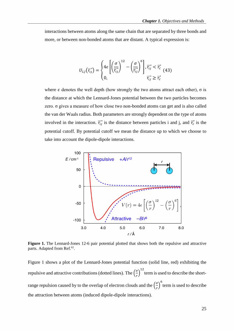
Dipole-Dipole interaction: A Lennard-Jones potential analyzes the hardcore repulsion
occurring at close distances due to the overlap of electron orbitals, and long-range
attraction at greater distances due to van der Waals interactions. It describes
Chapter 1. Objectives and Methods
25
interactions between atoms along the same chain that are separated by three bonds and
more, or between non-bonded atoms that are distant. A typical expression is:
𝑈𝐿𝐽(𝑟𝑖𝑗 ) = {4𝜖 [(
𝜎
𝑟𝑖𝑗 )
12
− (𝜎
𝑟𝑖𝑗 )
6
] , 𝑟𝑖𝑗 < 𝑟𝑐
0, 𝑟𝑖𝑗 ≥ 𝑟𝑐
(43)
where 𝜖 denotes the well depth (how strongly the two atoms attract each other), σ is
the distance at which the Lennard-Jones potential between the two particles becomes
zero. σ gives a measure of how close two non-bonded atoms can get and is also called
the van der Waals radius. Both parameters are strongly dependent on the type of atoms
involved in the interaction. 𝑟𝑖𝑗 is the distance between particles i and j, and 𝑟𝑐 is the
potential cutoff. By potential cutoff we mean the distance up to which we choose to
take into account the dipole-dipole interactions.
Figure 1. The Lennard-Jones 12-6 pair potential plotted that shows both the repulsive and attractive
parts. Adapted from Ref.62.
Figure 1 shows a plot of the Lennard-Jones potential function (solid line, red) exhibiting the
repulsive and attractive contributions (dotted lines). The (𝜎
𝑟)12
term is used to describe the short-
range repulsion caused by to the overlap of electron clouds and the (𝜎
𝑟)6
term is used to describe
the attraction between atoms (induced dipole-dipole interactions).

Modelling the DGEBA-EDA poly-epoxy and its reactivity towards copper: experimental and
numerical approach
26
With classical molecular mechanics, one can performed static calculations. But molecular
simulations taking into account time and temperature are needed to calculate properties that can
be compared to experimental counterparts. Additionally, it would help to describe mechanisms
at a microscopic scale, which are not often totally identified with experiments. There are two
main technics of molecular simulations: Molecular Dynamics (MD) and Monte Carlo63
simulations (MC). Classical MD simulations solve the equations of motions of Newton to
predict the time evolution of a system either by taking into account temperature and pressure
or relaxing the system in a given time. MC simulations are a rigorous tool to extrapolate
multiple configurations of a system by using the Boltzmann distribution at a given temperature
and to get large and realistic samplings. MC methods are often used in conjunction with MD
by creating a large number of configurations and by choosing the most stable we can then use
in the MD context to simulate a real system64.
1.3.2.1 The molecular Dynamics (MD) method
An MD simulation can reproduce the general behavior of matter in gas, liquid, and solid states.
MD is performed within a specified ensemble65. The ensemble name refers to the quantities
that are fixed by the users and held constant during calculations, i.e. the number of particles
(N), the volume (V), the temperature (T), the energy (E) and the pressure (P). The MD
simulation can be done for a system in the microcanonical NVE ensemble. The system is thus
isolated because there is no exchange (matter, heat, work) with the environment. Nevertheless,
energy is not a variable that can be regulated in real life experiments. Many experimental
observations are done at constant pressure and temperature, such that the system is no longer
isolated from its environment. Therefore, simulations are also often performed in the canonical
ensemble (NVT), and in the isothermal-isobaric ensemble (NPT), and in a variety of other
ensembles depending on the knowledge that is targeted. Other quantities that can be fixed
include enthalpy (H), and chemical potential (μ). Although these ensembles are the most
common, this list is not exhaustive.
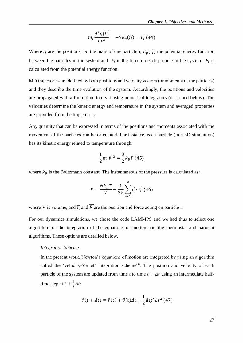
In Molecular Dynamics simulations the time evolution of a set of interacting particles is
followed via the solution of Newton’s equations of motion:
Chapter 1. Objectives and Methods
27
𝑚𝑖
𝜕2𝑟𝑖(𝑡)
𝜕𝑡2= −∇𝐸𝑝(𝑟 𝑖) = 𝐹𝑖 (44)
Where 𝑟 𝑖 are the positions, 𝑚𝑖 the mass of one particle i, 𝐸𝑝(𝑟 𝑖) the potential energy function
between the particles in the system and 𝐹𝑖 is the force on each particle in the system. 𝐹𝑖 is
calculated from the potential energy function.
MD trajectories are defined by both positions and velocity vectors (or momenta of the particles)
and they describe the time evolution of the system. Accordingly, the positions and velocities
are propagated with a finite time interval using numerical integrators (described below). The
velocities determine the kinetic energy and temperature in the system and averaged properties
are provided from the trajectories.
Any quantity that can be expressed in terms of the positions and momenta associated with the
movement of the particles can be calculated. For instance, each particle (in a 3D simulation)
has its kinetic energy related to temperature through:
1
2𝑚|𝑣 |2 =
3
2𝑘𝐵𝑇 (45)
where 𝑘𝐵 is the Boltzmann constant. The instantaneous of the pressure is calculated as:
𝑃 =𝑁𝑘𝐵𝑇
𝑉+
1
3𝑉∑𝑟𝑖 ∙ 𝐹𝑖
𝑁
𝑖=1
(46)
where V is volume, and 𝑟𝑖 and 𝐹𝑖 are the position and force acting on particle i.
For our dynamics simulations, we chose the code LAMMPS and we had thus to select one
algorithm for the integration of the equations of motion and the thermostat and barostat
algorithms. These options are detailed below.
Integration Scheme
In the present work, Newton’s equations of motion are integrated by using an algorithm
called the ‘velocity-Verlet’ integration scheme66. The position and velocity of each
particle of the system are updated from time t to time 𝑡 + 𝛥𝑡 using an intermediate half-
time step at 𝑡 +1
2𝛥𝑡:
𝑟 (𝑡 + 𝛥𝑡) = 𝑟 (𝑡) + 𝑣 (𝑡)𝛥𝑡 +1
2𝑎 (𝑡)𝛥𝑡2 (47)
Modelling the DGEBA-EDA poly-epoxy and its reactivity towards copper: experimental and
numerical approach
28
where 𝑎 (𝑡) is the acceleration of a particle at a time t. It is calculated from the force acting
on the particles divided by their mass. Δt is the timestep.
The velocities and positions are updated at half time step and at time step:
𝑣 (𝑡 +1
2𝛥𝑡) = 𝑣 (𝑡 −
1
2𝛥𝑡) 𝛥𝑡 + 𝑣 (𝑡)𝛥𝑡 (48)
𝑟 (𝑡 + 𝛥𝑡) = 𝑟 (𝑡) + 𝑣 (𝑡 +1
2𝛥𝑡) (49)
Using the updated positions and velocities each time, the force 𝐹 (𝑡 + 𝛥𝑡) is further
evaluated.
At t = 0 the initial velocities are given to the particles by using a Maxwell-Boltzmann
distribution corresponding to the fixed temperature. This integrator is fast, simple and
stable. The step-by-step execution of the algorithm is given in Annex B.
The timestep in the simulations needs to be validated by preliminary computations. In our
work, the choice of the timestep depends on the time required to observe the microscopic
evolution of the system (movements of molecules and chains). So it should be large
enough to capture the dynamics of the system. On the other hand, a very large timestep
(e.g. 1 ns) will lead to the immediate destruction of the simulation box as the forces
developed for a time evolution of this magnitude will cause overlaps of atoms.
Periodic conditions
We perform periodic computations in order to simulate a polymer bulk phase. It is thus
essential to choose periodic boundary conditions that mimic practically an infinite sample
of the material. The volume containing the N particles is treated as the primitive cell of
an infinite periodic lattice of identical cells. A given particle from the primitive cell
interacts with all other particles in this infinitely periodic system, i.e., with all other
particles in the same periodic cell and all particles (including its own periodic image) in
all other cells. Also, as a molecule leaves the central box, one of its images will enter
through the opposite face. There are no walls at the boundary of the central box, and no
surface molecules. Of course, since the poly-epoxy material is amorphous, one must

Chapter 1. Objectives and Methods
29
check that periodicity does not add order to the system that would bias calculated
properties.
Thermostat Algorithms
An algorithm that maintains a periodic simulation box at a fixed temperature is called a
thermostat algorithm65,67,68. A thermostat can be used to: (i) match experimental
conditions (most condensed-phase calculations are performed under temperature); (ii)
study temperature dependent processes (e.g., determination of thermal coefficients,
determination of glass transition temperature etc.) and (iii) enhance the efficiency of a
conformational search (e.g., high-temperature dynamics, simulated annealing). The use
of a thermostat requires the definition of an instantaneous temperature. This temperature
will be compared to the reference temperature To of the heat bath to which the system is
coupled. A good thermostat should reproduce the required temperature at our given
timescale at least qualitatively.
We choose the Nosé-Hoover thermostat65 for our NPT and NVT simulations because this
thermostat is deterministic and time-reversible. It will always satisfy the same dynamic
equations as when the system started to evolve.
The Nosé-Hoover thermostat works through the following equations:
𝑟𝑖 =𝑝𝑖
𝑚𝑖 (50)
𝑝𝑖 = 𝐹𝑖 (𝑟1 , … , 𝑟1 ) − 휁𝑝𝑖 (51)
휁 =1
𝑄[∑
𝑝 𝑖2
2𝑚𝑖𝑖
− 3𝑁𝑘𝐵𝑇] (52)
where ζ is a thermodynamic friction coefficient that allows the heat exchange between
the thermostat and our system. Q determines the strength of the thermostat. The
thermostat by using these equations allows us to acquire the statistical evolution of the
system in the canonical ensemble. Although comparing whether one thermostat leads to
a better description of the dynamics compared to another one is empirical, it seems
reasonable to assume that: (i) thermostats that allow the temperature to oscillate are more
likely to represent the dynamics correctly compared to thermostats fixing the temperature
Modelling the DGEBA-EDA poly-epoxy and its reactivity towards copper: experimental and
numerical approach
30
at a given value; (ii) thermostats with temperature fluctuations are more likely to represent
the dynamics correctly when these fluctuations occur in the duration of a simulation and
when the dynamics is smooth (continuous velocity trajectory).
Barostat Algorithms
An extension of the MD method to systems not described by the microcanonical NVE
ensemble was presented by Andersen67 in 1980. Andersen proved that by modifying the
Lagrangian of the system, a constant external pressure could be added in the MD
simulation of a system. Specifically for a system in which a constant external pressure P
is imposed, the system volume V is a dynamic variable that fluctuates in order to maintain
mechanical equilibrium between the external and system pressures. The system is then
exposed to a barostat, whereby an analogy of a “piston” of arbitrary “mass” as given by
textbooks, controls the dynamics of the volume. While ensemble averages are
independent of the piston mass, the fictitious mass does affect the response time for
volume fluctuations.
Andersen’s approach was later modified to simulate systems in contact with a
thermostat67. Nosé65 and Hoover69,70 proposed another isothermal-isobaric (NPT) MD
algorithm using a modification of Andersen’s piston method for maintaining constant
pressure and the thermostating method of Nosé. Later, other algorithms were developed
and the choice is again subjective to the results observed a given system. In general the
barostat will have much larger oscillations than a thermostat (a characteristic that we also
observed in the present work).
Our choice for a barostat is the Nosé-Hoover barostat69. It allows the volume of the system
to fluctuate under constant pressure. This algorithm drives the system to the state where
the average internal pressure is equal to the applied external pressure. It follows an
approach analogous to the Nosé-Hoover thermostat using a separate set of variables.
Chapter 1. Objectives and Methods
31
The LAMMPS simulation software
In this section, a description of the LAMMPS26 code is given, because this is the code
employed in the present MD simulations. The basic features and advantages of this code
can be summarized as follows:
LAMMPS is a classical molecular dynamics code. The acronym stands for Large-
scale Atomic/Molecular Massively Parallel Simulator.
LAMMPS integrates Newton's equations of motion for collections of atoms,
molecules, or macroscopic particles that interact via short- or long-range forces
with a variety of initial and/or boundary conditions. The integration of the
equations of motion can be done either with the velocity Verlet66 or the rRESPA71
algorithm.
It contains many potential functions in its libraries both for soft (biomolecules,
polymers) and solid-state (metals, semiconductors) materials, as well as for coarse
grained or mesoscopic systems. The Coulombic interactions are addressed by
many different methods such as the Ewald and the particle-particle-particle-mesh
(PPPM) methods.
LAMMPS proposes minimization algorithms such as steepest descent72 (SD),
Conjugate Gradient73 (CG), and Hessian Free-Truncated Newton74 (HFTN).
For NVT and NPT molecular dynamics simulations, the temperature is kept
constant either with the Berendsen68 or the Nosé-Hoover65 thermostats and the
pressure is kept constant with the Nosé-Hoover barostat65.
The biggest advantage of LAMMPS though, is that it is optimized in order to work
as efficiently as possible on parallel machines. LAMMPS uses spatial
decomposition techniques to partition the simulation domain into small 3D
subdomains, each one assigned to a different processor. Processors communicate
by using the message passing method via the MPI libraries.
Finally it is freely available and has an enormous community upon which
someone can rely for any troubleshooting that may occur.
Modelling the DGEBA-EDA poly-epoxy and its reactivity towards copper: experimental and
numerical approach
32
1.4 Computational Facilities
Calculations were executed on the EoS supercomputing cluster which belongs to the Scientific
Grouping CALMIP (Computations in Midi-Pyrénées75). EoS (Bull SA) comprises 12240 cores
and a total of 612 nodes for utilization by the users (612 nodes * 20 cores each). The processors
are Intel Xeon E5-2680v2 10C 2.8GHz which have 10 cores each with the ability to hyperthread
doubling the number of cores available in each node. It uses the Intel Math Kernel Library and
utilizes MPI (Message Passing Interface) and has Intel FORTRAN Compilers.
The deMon2k software suite was compiled using the MPI protocol on EoS in order to have the
capability to perform calculations using multiple cores and nodes thus increasing calculation
speed.
LAMMPS was build using the MPI protocol for parallelization allowing the use of multiple
cores and the g++ compiler available on EoS. For using special features (such as the PPPM
method) additional packages were installed that exist in the .tar file of LAMMPS.
1.5 Conclusion
We have seen in this chapter some basic elements of both quantum and classical theories that
are the basis of our calculations. We are going to analyze the results of our computations and
show how joining both quantum and classical approaches can lead to accurate simulation of the
XPS spectra of both the pristine and metalized surface as well as the bulk of our model poly-
epoxy polymer, in the following Chapters 3 (quantum simulations) and 4 (classical dynamics).
But first, Chapter 2 will introduce the experimental counterpart of the project. The synthesis
and characterization of poly-epoxy polymers and their surface metallization are presented
together with methods and techniques used.
Bibliography
1. Pascault, J. P., Sautereau, H., Verdu, J. & Williams, R. J. . Thermosetting Polymers. (CRC Press,
2002).
2. Petrie, E. M. Handbook of Adhesives and Sealants. (McGraw-Hill, 2007).
3. Gooch, J. W. Encyclopedic dictionary of polymers. (Springer, 2010).
4. Petrie, E. M. Epoxy adhesives formulation. (McGraw-Hill, 2006).
5. Charbonnier, M. & Romand, M. Polymer pretreatments for enhanced adhesion of metals deposited
by the electroless process. Int. J. Adhes. Adhes. 23, 277–285 (2003).
6. Baum, T. H., Miller, D. C. & O’Toole, T. R. Photoselective catalysis of electroless copper solutions
for the formation of adherent copper films onto polyimide. Chem. Mater. 3, 714–720 (1991).

Chapter 1. Objectives and Methods
33
7. Yoon, S., Choi, H.-J., Yang, J.-K. & Park, H.-H. Comparative study between poly(p-
phenylenevinylene) (PPV) and PPV/SiO2 nano-composite for interface with aluminum electrode.
Appl. Surf. Sci. 237, 451–456 (2004).
8. Woo, T.-G., Park, I.-S. & Seol, K.-W. Effects of various metal seed layers on the surface
morphology and structural composition of the electroplated copper layer. Met. Mater. Int. 15, 293–
297 (2009).
9. E. Sacher (ed.). Metallization of Polymers 2. (Plenum Publishers, 2002).
10. Kanzow, J. et al. Formation of a metal/epoxy resin interface. Appl. Surf. Sci. 239, 227–236 (2005).
11. LeGoues, F. K., Silverman, B. D. & Ho, P. S. The microstructure of metal–polyimide interfaces. J.
Vac. Sci. Technol. A 6, 2200–2204 (1988).
12. Davis, G. D., Rees, B. J. & Whisnant, P. L. Chemical evaluation of Cu–polyimide interfaces. J.
Vac. Sci. Technol. A 12, 2378–2387 (1994).
13. Pertsin, A. J. & Pashunin, Y. M. An XPS study of the in-situ formation of the polyimide/copper
interface. Appl. Surf. Sci. 47, 115–125 (1991).
14. Bébin, P. & Prud’homme, R. E. Comparative XPS Study of Copper, Nickel, and Aluminum
Coatings on Polymer Surfaces. Chem. Mater. 15, 965–973 (2003).
15. Wolany, D. et al. Combined ToF-SIMS/XPS study of plasma modification and metallization of
polyimide. Surf. Interface Anal. 27, 609–617 (1999).
16. Haight, R., White, R. C., Silverman, B. D. & Ho, P. S. Complex formation and growth at the Cr–
and Cu–polyimide interface. J. Vac. Sci. Technol. Vac. Surf. Films 6, 2188–2199 (1988).
17. Bartha, J. W., Hahn, P. O., LeGoues, F. & Ho, P. S. Photoemission spectroscopy study of
aluminum–polyimide interface. J. Vac. Sci. Technol. Vac. Surf. Films 3, 1390–1393 (1985).
18. Travaly, Y., Bertrand, P., Rignanese, G.-M. & Gonze, X. Theoretical Modeling of the Nucleation
and Growth of Aluminium Films Thermally Evaporated onto Poly(ethylene terephthalate)
Substrate. J. Adhes. 66, 339–355 (1998).
19. Travaly, Y. & Bertrand, P. Static SIMS investigation of metal/polymer interfaces. Surf. Interface
Anal. 23, 328–334 (1995).
20. Siau, S., Vervaet, A., Degrendele, L., Baets, J. D. & Calster, A. V. Qualitative electroless Ni/Au
plating considerations for the solder mask on top of sequential build-up layers. Appl. Surf. Sci. 252,
2717–2740 (2006).
21. Sykes, J. M. & Hoar, T. P. Role of polymer oxidation in the adhesion of polyethylene to metals. J.
Polym. Sci. [A1] 7, 1385–1391 (1969).
22. Mittal, K. L. Adhesion aspects of metallization of organic polymer surfaces. J. Vac. Sci. Technol.
13, 19–25 (1976).
23. Derjaguin, B. V. & Smilga, V. P. Electronic Theory of Adhesion. J. Appl. Phys. 38, 4609–4616
(1967).
24. Skinner, S. M., Savage, R. L. & Jr, J. E. R. Electrical Phenomena in Adhesion. I. Electron
Atmospheres in Dielectrics. J. Appl. Phys. 24, 438–450 (1953).
25. Binder, K. Monte Carlo and Molecular Dynamics Simulations in Polymer Science. (Oxford
University Press, 1995).
26. Plimpton, S. Fast Parallel Algorithms for Short-Range Molecular Dynamics. J. Comput. Phys. 117,
1–19 (1995).
27. Kalé, L. et al. NAMD2: Greater Scalability for Parallel Molecular Dynamics. J. Comput. Phys. 151,
283–312 (1999).
28. Rudd, R. E. & Broughton, J. Q. Coarse-grained molecular dynamics and the atomic limit of finite
elements. Phys. Rev. B 58, R5893–R5896 (1998).
29. Padding, J. T. & Briels, W. J. Time and length scales of polymer melts studied by coarse-grained
molecular dynamics simulations. J. Chem. Phys. 117, 925–943 (2002).
30. Hohenberg, P. & Kohn, W. Inhomogeneous Electron Gas. Phys. Rev. 136, B864–B871 (1964).
31. Kohn, W. & Sham, L. J. Self-Consistent Equations Including Exchange and Correlation Effects.
Phys. Rev. 140, A1133–A1138 (1965).
32. Perdew, J. P. & Zunger, A. Self-interaction correction to density-functional approximations for
many-electron systems. Phys. Rev. B 23, 5048–5079 (1981).
33. Vosko, S. H., Wilk, L. & Nusair, M. Accurate spin-dependent electron liquid correlation energies
for local spin density calculations: a critical analysis. Can. J. Phys. 58, 1200–1211 (1980).

Modelling the DGEBA-EDA poly-epoxy and its reactivity towards copper: experimental and
numerical approach
34
34. Ceperley, D. M. & Alder, B. J. Ground State of the Electron Gas by a Stochastic Method. Phys.
Rev. Lett. 45, 566–569 (1980).
35. Kohanoff, J. Electronic Structure Calculations for Solids and Molecules: Theory and Computational
methods. Cambridge University Press Available at:
http://www.cambridge.org/fr/academic/subjects/physics/condensed-matter-physics-nanoscience-
and-mesoscopic-physics/electronic-structure-calculations-solids-and-molecules-theory-and-
computational-methods. (Accessed: 15th October 2017)
36. Jacobsen, H. & Cavallo, L. Directions for Use of Density Functional Theory: A Short Instruction
Manual for Chemists. in Handbook of Computational Chemistry (ed. Leszczynski, J.) 95–133
(Springer Netherlands, 2012). doi:10.1007/978-94-007-0711-5_4
37. Lee, C., Yang, W. & Parr, R. G. Development of the Colle-Salvetti correlation-energy formula into
a functional of the electron density. Phys. Rev. B 37, 785–789 (1988).
38. Perdew, J. P. et al. Atoms, molecules, solids, and surfaces: Applications of the generalized gradient
approximation for exchange and correlation. Phys. Rev. B 46, 6671–6687 (1992).
39. Perdew, J. P., Burke, K. & Ernzerhof, M. Generalized Gradient Approximation Made Simple. Phys.
Rev. Lett. 77, 3865–3868 (1996).
40. Csonka, G. I., Perdew, J. P. & Ruzsinszky, A. Global Hybrid Functionals: A Look at the Engine
under the Hood. J. Chem. Theory Comput. 6, 3688–3703 (2010).
41. Becke, A. D. Density‐functional thermochemistry. III. The role of exact exchange. J. Chem. Phys.
98, 5648–5652 (1993).
42. Heyd, J., Scuseria, G. E. & Ernzerhof, M. Hybrid functionals based on a screened Coulomb
potential. J. Chem. Phys. 118, 8207–8215 (2003).
43. Kostar, A. M. et al. A.M. Koster, G. Geudtner, P. Calaminici, M.E. Casida, V.D. Dominguez, R.
Flores-Moreno, G.U. Gamboa, A. Goursot, T. Heine, A. Ipatov, F. Janetzko, J.M. del Campo, J. U.
Reveles, A. Vela, B. Zuniga-Gutierrez, and D.R. Salahub, deMon2k, Version 3.0.6, The deMon
developers, Cinvestav, Mexico City (2011). (2014).
44. St-Amant, A. deMon, un programme LCGTO-MCP-DF, et une etude théorique de l’adsorption de
l’hydrogène sur les monomères et dimères de Ni, Rh, et Pd. (Université de Montréal, 1992).
45. Eichkorn, K., Treutler, O., Öhm, H., Häser, M. & Ahlrichs, R. Auxiliary basis sets to approximate
Coulomb potentials. Chem. Phys. Lett. 240, 283–290 (1995).
46. Dunlap, B. I., Connolly, J. W. D. & Sabin, J. R. On first‐row diatomic molecules and local density
models. J. Chem. Phys. 71, 4993–4999 (1979).
47. Mintmire, J. W. & Dunlap, B. I. Fitting the Coulomb potential variationally in linear-combination-
of-atomic-orbitals density-functional calculations. Phys. Rev. A 25, 88–95 (1982).
48. Mintmire, J. W., Sabin, J. R. & Trickey, S. B. Local-density-functional methods in two-
dimensionally periodic systems. Hydrogen and beryllium monolayers. Phys. Rev. B 26, 1743–1753
(1982).
49. Köster, A. M. Hermite Gaussian auxiliary functions for the variational fitting of the Coulomb
potential in density functional methods. J. Chem. Phys. 118, 9943–9951 (2003).
50. Geudtner, G. et al. deMon2k. Wiley Interdiscip. Rev. Comput. Mol. Sci. 2, 548–555 (2012).
51. Calaminici, P. et al. Auxiliary Density Functional Theory: From Molecules to Nanostructures. in
Handbook of Computational Chemistry 575–610
52. Salahub, D. R., Goursot, A., Weber, J., Köster, A. M. & Vela, A. Chapter 38 - Applied density
functional theory and the deMon codes 1964–2004. in Theory and Applications of Computational
Chemistry (eds. Dykstra, C. E., Frenking, G., Kim, K. S. & Scuseria, G. E.) 1079–1097 (Elsevier,
2005). doi:10.1016/B978-044451719-7/50081-0
53. Institute for Theoretical Chemistry | Institut für Theoretische Chemie | University of Stuttgart.
Available at: http://www.uni-stuttgart.de/theochem/. (Accessed: 29th September 2017)
54. Schuchardt, K. L. et al. Basis Set Exchange: A Community Database for Computational Sciences.
J. Chem. Inf. Model. 47, 1045–1052 (2007).
55. Halgren, T. A. & Damm, W. Polarizable force fields. Curr. Opin. Struct. Biol. 11, 236–242 (2001).

Chapter 1. Objectives and Methods
35
56. van Duin, A. C. T., Dasgupta, S., Lorant, F. & Goddard, W. A. ReaxFF: A Reactive Force Field
for Hydrocarbons. J. Phys. Chem. A 105, 9396–9409 (2001).
57. Barnoud, J. & Monticelli, L. Coarse-Grained Force Fields for Molecular Simulations. in Molecular
Modeling of Proteins (ed. Kukol, A.) 1215, 125–149 (Springer New York, 2015).
58. Wang, J., Wolf, R. M., Caldwell, J. W., Kollman, P. A. & Case, D. A. Development and testing of
a general amber force field. J. Comput. Chem. 25, 1157–1174 (2004).
59. D.A. Case, D.S. Cerutti, T.E. Cheatham, III, T.A. Darden, R.E. Duke, T.J. Giese, H. Gohlke, A.W.
Goetz, D. Greene, N. Homeyer, S. Izadi, A. Kovalenko, T.S. Lee, S. LeGrand, P. Li, C. Lin, J. Liu,
T. Luchko, R. Luo, D. Mermelstein, K.M. Merz, G. Monard, H. Nguyen, I. Omelyan, A. Onufriev,
F. Pan, R. Qi, D.R. Roe, A. Roitberg, C. Sagui, C.L. Simmerling, W.M. Botello-Smith, J. Swails,
R.C. Walker, J. Wang, R.M. Wolf, X. Wu, L. Xiao, D.M. York and P.A. Kollman (2017), AMBER
2017, University of California, San Francisco.
60. Del Buono, G. S., Figueirido, F. E. & Levy, R. M. Dielectric response of solvent surrounding an
ion pair: Ewald potential versus spherical truncation. Chem. Phys. Lett. 263, 521–529 (1996).
61. Hockney, R. & Eastwood, J. Particle-Particle-Particle-Mesh (P3M) Algorithms. in Computer
simulation using particles 267–304
62. Lennard Jones Potential Equation - Jennarocca. Available at: http://jennarocca.com/lennard-jones-
potential-equation/. (Accessed: 4th September 2017)
63. Metropolis, N. & Ulam, S. The Monte Carlo Method. J. Am. Stat. Assoc. 44, 335–341 (1949).
64. Chiu, S. W., Jakobsson, E., Subramaniam, S. & Scott, H. L. Combined Monte Carlo and Molecular
Dynamics Simulation of Fully Hydrated Dioleyl and Palmitoyl-oleyl Phosphatidylcholine Lipid
Bilayers. Biophys. J. 77, 2462–2469 (1999).
65. Nosé, S. A unified formulation of the constant temperature molecular dynamics methods. J. Chem.
Phys. 81, 511–519 (1984).
66. Verlet, L. Computer ‘Experiments’ on Classical Fluids. I. Thermodynamical Properties of Lennard-
Jones Molecules. Phys. Rev. 159, 98–103 (1967).
67. Andersen, H. C. Molecular dynamics simulations at constant pressure and/or temperature. J. Chem.
Phys. 72, 2384–2393 (1980).
68. Ryckaert, J.-P., Ciccotti, G. & Berendsen, H. J. C. Numerical integration of the cartesian equations
of motion of a system with constraints: molecular dynamics of n-alkanes. J. Comput. Phys. 23, 327–
341 (1977).
69. Hoover, W. G. & Holian, B. L. Kinetic moments method for the canonical ensemble distribution.
Phys. Lett. A 211, 253–257 (1996).
70. Alder, B. J., Hoover, W. G. & Young, D. A. Studies in Molecular Dynamics. V. High‐Density
Equation of State and Entropy for Hard Disks and Spheres. J. Chem. Phys. 49, 3688–3696 (1968).
71. Plimpton, S., Pollock, R. & Stevens, M. Particle-Mesh Ewald and rRESPA for Parallel Molecular
Dynamics Simulations. in In Proceedings of the Eighth SIAM Conference on Parallel Processing
for Scientific Computing (1997).
72. Goldstein, A. On Steepest Descent. J. Soc. Ind. Appl. Math. Ser. Control 3, 147–151 (1965).
73. Ajiz, M. A. & Jennings, A. A robust incomplete Choleski-conjugate gradient algorithm. Int. J.
Numer. Methods Eng. 20, 949–966 (1984).
74. Chapelle, O. & Erhan, D. Improved preconditioner for hessian free optimization. in In NIPS
Workshop on Deep Learning and Unsupervised Feature Learning (2011).
75. CALMIP. Available at: https://www.calmip.univ-toulouse.fr/. (Accessed: 29th September 2017)


Chapter 2: Experimental formation of model poly-epoxy surfaces and characterizations
37
Chapter 2: Experimental formation of model poly-epoxy surfaces
and characterizations
2.1 Introduction
Poly-epoxy polymers are of tremendous interest in various industrial sectors and are involved
in various ongoing researches for their surface or bulk functionalization. Examples of
applications are found in the leisure industry, or the aerospace and military industry1–4. Poly-
epoxies are traditionally used as adhesives, sealants, or paints, and as the matrix in composites
because of their superior thermal and mechanical properties when compared to other polymers.
In fact, poly-epoxies cover 80% of the general demand of polymers for high performance
composites5. Main reinforcements are carbon fibers. But for the latter application, it may be
necessary to proceed to a metallization as in the present project.
Epoxy resins used as commercial products contain aliphatic, cycloaliphatic or aromatic
backbones. Their molecular weights can be adjusted from a few hundreds to tens of thousands.
The most widely used epoxy resins are the glycidyl ether derivatives of bisphenol A (more than
75% of total resin sales), such as the diglycidylether of bisphenol A (DGEBA) of the present
study. The epoxy rings of DGEBA can react with a wide variety of curing agents. Here, we use
ethylene diamine (EDA) which is the smallest liquid amine.
As we described in the previous chapter, poly-epoxy surfaces we form are intended to be
metallized at ambient temperature under ultrahigh vacuum (UHV) conditions. Metallized
polymers have a great variety of applications (e.g. in the microelectronics sector)and thus the
analysis of the chemical bonds formed and reaction at these interfaces have a great interest6–8.
In our works, we are interested in analyzing the poly-epoxy/metal interface9–11. In the literature,
Wagner et al.12 investigated the reactivity of Fe, Ni, Cu, and Au evaporated in UHV on 3
different N-containing polymers (Nylon 6 which contains C=O and C-N functionalities, N-PE
with different C-N, and CN-SAM which only exhibits C≡N nitriles). Overall it is shown that
the reactivity order Fe>Ni>Cu>Au follows the affinity of the metals for O and N.
A very important tool to aid us in our objective is the polymer/metal X-Ray Photoelectron
Spectroscopy used for surface chemical analysis. Our aim is to get an insight in the mechanisms
of formation of polymer/metal interfaces, which depend on three main features13,14: (i) the
availability of reactive functional groups at the polymer surface, (ii) the nano- and
Modelling the DGEBA-EDA poly-epoxy and its reactivity towards copper: experimental and
numerical approach
38
microstructure of the surface, and (iii) the valence of the metal adsorbate(s). Metals that easily
form oxides, such as Al, Cr, Fe, or Ni, will form stable metal (M-)O-C covalent bonds12,15–17.
On a poly-epoxy that is similar to the one of the present work, observations of condensation
coefficients, bonding, and diffusion of Al, Cu, Ag, and Au show the same trend for reactivities:
Al >Cu>Au>Ag18. Al oxidizes and forms a dense layer, whereas Cu, Au, and Ag form clusters.
Diffusion towards the bulk is negligible, even above glass transition temperature, in contrast
with metal/thermoplastics interfaces. Finally, when the adsorption is accompanied by a
degradation of the polymer chain by scissions, the most reactive metals (e.g. Cr or Ni) form
carbides or phosphides15.
Chapter 2 is organized as follows: Section 2 is dedicated to the presentation of the synthesis
and characterization of the poly-epoxy polymer bulk as well as the pristine surface. The
synthesis protocol is presented, followed by the FTIR and DSC measurements. The surface is
also characterized by AFM and XPS measurements. Following, in section 3, we describe the
protocol of the deposition of a Cu film on the poly-epoxy surface. AFM measurements are
executed for the calibration of the time of deposition through metallization of Si wafers in
different times and for the determination of the thickness of the Cu film deposited on the poly-
epoxy surface. Lastly XPS measurements give us a first indication for the mechanism of
reaction of the Cu atoms with the surface functions.
2.2 Pristine (non-metallized) poly-epoxy surface
2.2.1 Synthesis protocol of a pristine low-roughness poly-epoxy surface
The first step is to be able to accurately and reproducibly create a surface with very low
roughness (Ra<1 nm) so that we are able to observe nano-clusters and nano-islands
formation without any prevention or confusion with roughness existing on the surface.
Another reason for a surface with a low defect density is to ensure that heterogeneous
nucleation will not take place in these defects. Finally, our samples must be chemically
homogeneous since chemical homogeneity is assumed in calculations. At the end of a period
of tedious research (described in section 2.2) we have finally developed a safe protocol that
ensures all samples of a batch to be close to full polymerization (~ 93%).

Chapter 2: Experimental formation of model poly-epoxy surfaces and characterizations
39
The protocol involves the following steps:
The Si wafer substrates along with any disposable and non-disposable tools that will
be used are thoroughly cleaned and dried with ethanol and/or acetone depending on
the material.
After everything is dried it is carefully placed in the load-lock chamber of an Ar
glovebox for overnight pumping.
In the Ar glovebox, we mix 0.86 g of EDA and 10 g of DGEBA (stoichiometric
2DGEBA:1EDA mixture).
The liquid mixture is stirred manually using a plastic or wooden stirrer for 7 minutes
for a homogeneous stirring.
Then, small droplets are deposited on the clean Si wafers. They are left for 48h in
the Ar glovebox in order to reach approx. 80% conversion rate.
After the 48h period, an electric heater is used for post-curing (2h, 140°C).
In section 2.2.2.1 we describe bulk properties and how we determine the polymerization rate
based on Fourier-transform infrared spectroscopy (FTIR), and how we determine the glass
transition temperature (Tg) by differential scanning calorimetry (DSC). We also ensure that the
surface has the required low roughness using atomic force microscopy (AFM) and obtain
surface chemical composition by analyzing X-Ray photoelectron spectra (XPS).
2.2.2. Characterizations
2.2.2.1 Bulk Characterizations
Introduction to Fourier Transform Infrared (FTIR) spectroscopy
Fourier Transform Infrared (FTIR) spectroscopy is a very useful analytical tool. It is a
technique in which we obtain an infrared spectrum of absorption or emission of a material
in any phase (gas, liquid or solid). For our project we need to analyze solid (our final
polymers) and liquid (initial mixture of DGEBA and EDA). We will speak briefly about
the methodology and functionality of FTIR spectroscopy before showing our results.
Generally speaking, an absorption spectroscopy technique (such as FTIR, UV-Vis
(ultraviolet-visible), photoemission spectroscopy etc.) outputs a spectra that shows the
ability of the material to absorb light at a great number of wavelengths. The simplest way

Modelling the DGEBA-EDA poly-epoxy and its reactivity towards copper: experimental and
numerical approach
40
to do this is to use a monochromatic light source at a given sample and then repeat for
various wavelengths.
Fourier-transform spectroscopy accelerates this procedure by the use of a polychromatic
source and records the percentage of the beam that is either absorbed or transmitted,
depending on the modes the user selects or the material nature (e.g. how transparent the
material is). The beams emitted are of certain bandwidths and thus one can scan a large
range of frequencies. We use transmission IR spectroscopy in the Near Infrared (NIR)
spectrum. The apparatus is the Perkin Elmer Frontier and Spotlight NIR/MIR spectrometer.
In order to calculate the conversion rate (Xe,NIR), we use Equation 1:
𝑋𝑒,𝑁𝐼𝑅 = 1 −
(𝐴𝑒𝑝𝑜𝑥𝑦
𝐴𝑟𝑒𝑓𝑒𝑟𝑒𝑛𝑐𝑒)
𝑡
(𝐴𝑒𝑝𝑜𝑥𝑦
𝐴𝑟𝑒𝑓𝑒𝑟𝑒𝑛𝑐𝑒)
𝑡=0
(1)
As indicated in the equation we extract spectra in the near infrared (NIR) area of the
spectrum. The terms Aepoxy and Areference refer to the area of the peak of the epoxy bond
located in the 4530 cm-1 band, and the area of the reference band (combination of the
aromatic C=C (1625 cm-1) and aromatic C-H (3000 cm-1) bond) located at 4623 cm-1.19,20
We obtain background spectra by using two empty microscope glass slides.
Results of FTIR characterizations
In our project, FTIR spectroscopy is useful to ensure that the reaction of polymerization
takes place, and enables the determination of the conversion rate (%). It is important that
all samples are close to 100% polymerization. The reason is not only the relevance with
DFT and Molecular Dynamics calculations but also the compatibility of the samples with
UHV. They will be introduced in the XPS apparatus (10-9 mbar) and in the evaporation
chamber (10-10 mbar) for metallization. If samples are not completely solid then the UHV
chambers will be contaminated.
In order to have a rigorous polymerization protocol, results from previous works are used21
to help us determine the time needed for the samples to stay in the Ar gloves box until the
maximum conversion rate has been reached in ambient temperature. The findings of this
work described in Figures 1 and 2 indicate that the minimum time the samples need to stay

Chapter 2: Experimental formation of model poly-epoxy surfaces and characterizations
41
in ambient temperature under Ar atmosphere is 48h. After the 48h period there is no
significant change in the conversion rate and a post-curing at higher temperatures is needed.
Figure 1 shows the superposition of 6 FTIR spectra acquired from t=0 to t > 8 days.
Figure 1. Polymerization monitoring by the use of FTIR adapter from Ref.22
The time of the initial mixing of the DGEBA and EDA reactants is denoted as t=0. For
each time period, that the spectra are extrapolated in this study, it can be seen that while
the reference band remains constant, the epoxy band is continually lessened. Between the
24h spectrum and the 8 days spectrum the epoxy band does not have a significant difference
in peak size. The conversion rate has reached a plateau between this timespan. The spectra
acquired demonstrate the minimum amount possible of noise and the bands of interest can
be clearly identified. For each spectrum obtained, the areas of the bands are used as
constants for the subsequent calculations of Xe,NIR through Equation 1. The results of the
study concerning this parameter are given in Figure 2.
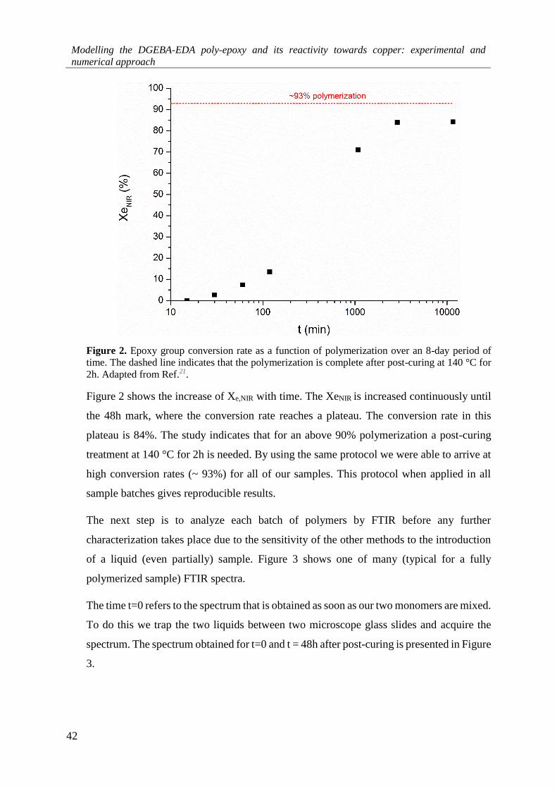
Modelling the DGEBA-EDA poly-epoxy and its reactivity towards copper: experimental and
numerical approach
42
Figure 2. Epoxy group conversion rate as a function of polymerization over an 8-day period of
time. The dashed line indicates that the polymerization is complete after post-curing at 140 °C for
2h. Adapted from Ref.21.
Figure 2 shows the increase of Xe,NIR with time. The XeNIR is increased continuously until
the 48h mark, where the conversion rate reaches a plateau. The conversion rate in this
plateau is 84%. The study indicates that for an above 90% polymerization a post-curing
treatment at 140 °C for 2h is needed. By using the same protocol we were able to arrive at
high conversion rates (~ 93%) for all of our samples. This protocol when applied in all
sample batches gives reproducible results.
The next step is to analyze each batch of polymers by FTIR before any further
characterization takes place due to the sensitivity of the other methods to the introduction
of a liquid (even partially) sample. Figure 3 shows one of many (typical for a fully
polymerized sample) FTIR spectra.
The time t=0 refers to the spectrum that is obtained as soon as our two monomers are mixed.
To do this we trap the two liquids between two microscope glass slides and acquire the
spectrum. The spectrum obtained for t=0 and t = 48h after post-curing is presented in Figure
3.
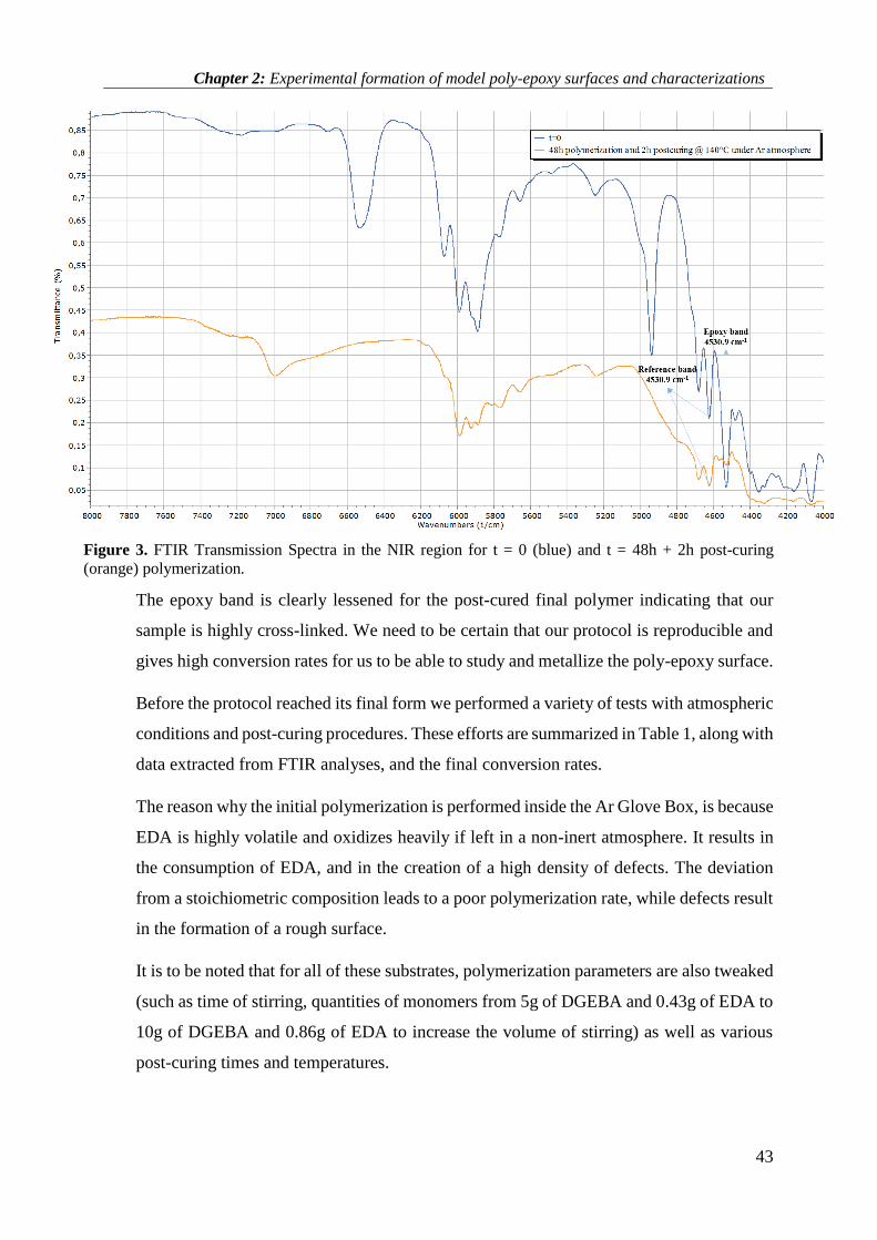
Chapter 2: Experimental formation of model poly-epoxy surfaces and characterizations
43
Figure 3. FTIR Transmission Spectra in the NIR region for t = 0 (blue) and t = 48h + 2h post-curing
(orange) polymerization.
The epoxy band is clearly lessened for the post-cured final polymer indicating that our
sample is highly cross-linked. We need to be certain that our protocol is reproducible and
gives high conversion rates for us to be able to study and metallize the poly-epoxy surface.
Before the protocol reached its final form we performed a variety of tests with atmospheric
conditions and post-curing procedures. These efforts are summarized in Table 1, along with
data extracted from FTIR analyses, and the final conversion rates.
The reason why the initial polymerization is performed inside the Ar Glove Box, is because
EDA is highly volatile and oxidizes heavily if left in a non-inert atmosphere. It results in
the consumption of EDA, and in the creation of a high density of defects. The deviation
from a stoichiometric composition leads to a poor polymerization rate, while defects result
in the formation of a rough surface.
It is to be noted that for all of these substrates, polymerization parameters are also tweaked
(such as time of stirring, quantities of monomers from 5g of DGEBA and 0.43g of EDA to
10g of DGEBA and 0.86g of EDA to increase the volume of stirring) as well as various
post-curing times and temperatures.
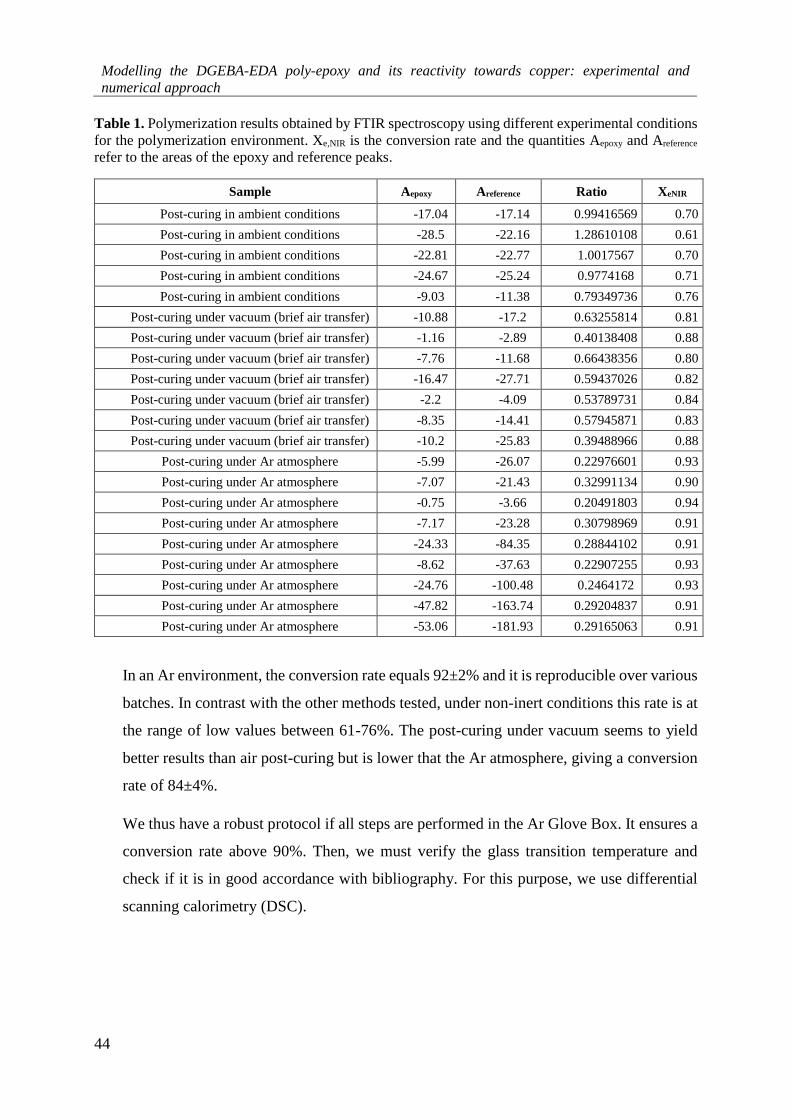
Modelling the DGEBA-EDA poly-epoxy and its reactivity towards copper: experimental and
numerical approach
44
Table 1. Polymerization results obtained by FTIR spectroscopy using different experimental conditions
for the polymerization environment. Xe,NIR is the conversion rate and the quantities Aepoxy and Areference
refer to the areas of the epoxy and reference peaks.
Sample Aepoxy Areference Ratio XeNIR
Post-curing in ambient conditions -17.04 -17.14 0.99416569 0.70
Post-curing in ambient conditions -28.5 -22.16 1.28610108 0.61
Post-curing in ambient conditions -22.81 -22.77 1.0017567 0.70
Post-curing in ambient conditions -24.67 -25.24 0.9774168 0.71
Post-curing in ambient conditions -9.03 -11.38 0.79349736 0.76
Post-curing under vacuum (brief air transfer) -10.88 -17.2 0.63255814 0.81
Post-curing under vacuum (brief air transfer) -1.16 -2.89 0.40138408 0.88
Post-curing under vacuum (brief air transfer) -7.76 -11.68 0.66438356 0.80
Post-curing under vacuum (brief air transfer) -16.47 -27.71 0.59437026 0.82
Post-curing under vacuum (brief air transfer) -2.2 -4.09 0.53789731 0.84
Post-curing under vacuum (brief air transfer) -8.35 -14.41 0.57945871 0.83
Post-curing under vacuum (brief air transfer) -10.2 -25.83 0.39488966 0.88
Post-curing under Ar atmosphere -5.99 -26.07 0.22976601 0.93
Post-curing under Ar atmosphere -7.07 -21.43 0.32991134 0.90
Post-curing under Ar atmosphere -0.75 -3.66 0.20491803 0.94
Post-curing under Ar atmosphere -7.17 -23.28 0.30798969 0.91
Post-curing under Ar atmosphere -24.33 -84.35 0.28844102 0.91
Post-curing under Ar atmosphere -8.62 -37.63 0.22907255 0.93
Post-curing under Ar atmosphere -24.76 -100.48 0.2464172 0.93
Post-curing under Ar atmosphere -47.82 -163.74 0.29204837 0.91
Post-curing under Ar atmosphere -53.06 -181.93 0.29165063 0.91
In an Ar environment, the conversion rate equals 92±2% and it is reproducible over various
batches. In contrast with the other methods tested, under non-inert conditions this rate is at
the range of low values between 61-76%. The post-curing under vacuum seems to yield
better results than air post-curing but is lower that the Ar atmosphere, giving a conversion
rate of 84±4%.
We thus have a robust protocol if all steps are performed in the Ar Glove Box. It ensures a
conversion rate above 90%. Then, we must verify the glass transition temperature and
check if it is in good accordance with bibliography. For this purpose, we use differential
scanning calorimetry (DSC).

Chapter 2: Experimental formation of model poly-epoxy surfaces and characterizations
45
Introduction to Differential Scanning Calorimetry (DSC)
DSC is a thermal analysis technique which measures the heating power absorbed or
produced by a sample when it is submitted to a heating or cooling profile. With a known
mass of material, DSC can determine heat capacity (cp) changes with temperature.
The glass transition temperature (Tg) is a characteristic temperature of poly-epoxies. Tg, is
the temperature for which the polymer changes from its glassy (low T) state to a rubbery
(higher T) state, accompanied by a significant change of its heat capacity (cp). Below Tg,
the cross-linked chains are very rigid and no mobility is permitted because of Van der
Waals (VdW) intermolecular interactions. At T>Tg the chains have enough energy to break
VdW bonds and to enter the rubbery state.
After weighting the required quantity of polymer, we seal it in an Al capsule using a pastille
maker. We also prepare a reference capsule that remains empty. The DSC apparatus
measures the heat flow of the two capsules and calculates the extra heat necessary to heat
the polymer-filled capsule at every temperature step so that the two capsules heat flows
remain constant. Through this method, we can calculate cp using Equations 2-4. In these
equations Φ is the heat flow, q represents heat, t is the time and ∆𝑇 is the variation of the
temperature for time t. We use a Netzsch DSC 204 apparatus to perform DSC experiments.
Φ =𝑞
𝑡(2)
𝑡𝑒𝑚𝑝𝑒𝑟𝑎𝑡𝑢𝑟𝑒 𝑣𝑎𝑟𝑖𝑎𝑡𝑖𝑜𝑛
𝑡𝑖𝑚𝑒=
∆𝑇
𝑡 (3)
𝑞𝑡
∆𝑇𝑡
=𝑞
∆𝑇= 𝐶𝑝 (4)
Glass transition temperature of the poly-epoxy
Figure 4 shows the DSC plot obtained with the following procedure. 11.8 mg of poly-epoxy
are placed in the capsule. Then, the chamber is heated from -10 to 250 °C, at a heating rate
of 10 °C/min. Reactions take place in an inert atmosphere composed of nitrogen which has
a high heat conductivity (0.026 W/m ∙ K) allowing the even distribution of heat in the
sample chamber. Argon is also a very good candidate although more expensive and is
preferred for high temperatures which is not needed for our polymer.

Modelling the DGEBA-EDA poly-epoxy and its reactivity towards copper: experimental and
numerical approach
46
In Figure 4, we observe an exothermic process, i.e. a decrease of the power injected in the
reactor chamber to maintain the temperature. The onset, midpoint and endpoint of the
transition are determined by post-processing; through the drawing of the tangents of the
glassy and rubbery regions. . We choose the mid-point temperature 118±1 °C (391±1 K)
as a Tg, because it is usually preferred in the bibliography23. The Tg presented in Figure 4
is obtained on 2 samples, with a margin of error of ±1 °C (the margin of error for the Indium
Response Ratio, used for calibration is ±0.5 °C and we have added a user error of fitting at
±0.5 °C). The results are in accordance with bibliography.23,24
After verifying the Tg of our polymers, and being sure that we have well polymerized
samples, we move on to the surface analysis of pristine surfaces using AFM and XPS.
Figure 4. DSC plot of a 93% polymerized poly-epoxy polymer.

Chapter 2: Experimental formation of model poly-epoxy surfaces and characterizations
47
2.2.2.2 Surface Characterizations
Introduction to Atomic Force Microscopy (AFM)
AFM is based on the interactions between a sharp tip and a surface. The probed interactions
are, from far to close tip, the electrostatic forces, the surface tension, and the coulombic
repulsion.
AFM has the advantage over scanning tunneling microscopy that it can give results for
both conducting and insulating surfaces, and measurements can be performed in ambient
air, liquid or vacuum. An example of application is the measurement of force-distance
curves.
There has been a great variety of scientific works in the last years whose aim was to
determine the viscoelastic behavior and the glass transition temperature Tg by the use of
force-distance curves. One example is the work of Marti et al.25 who used polystyrene
samples of different weights at different temperatures. They were able to measure the tip-
sample adhesion and found a large increase of adhesion above a specific temperature which
they assume to be Tg. Tsui et al26 examined force-distance curves at various temperatures
on poly(t-butyl acrylate) and showed the good agreement between the shift factors
(correcting the force-distance curves taking into account temperature) obtained using AFM
and rheological measurements (fracture mechanics at unloading) made on the bulk
polymer. The technical principles of AFM are described in Figure 5. The main component
is the cantilever. At its end, it has a sharp micro fabricated tip, with a radius of only a few
nanometers. The cantilever is usually made out of silicon or silicon nitride. The cantilever’s
back side (the side not in contact with samples) is covered with a thin metallic layer (e.g.
Au) in order to enhance its reflectivity. There, a laser beam is reflected toward a 2-
dimensional photodetector. When the cantilever moves because of tip-surface interactions,
then the reflection of the laser beam moves within the photodetector area. Lateral
movements correspond to tip flexion (i.e. friction) whereas vertical movements correspond
to z-motion (topography and/or repulsive/attractive interactions).

Modelling the DGEBA-EDA poly-epoxy and its reactivity towards copper: experimental and
numerical approach
48
Figure 5. Principle of Atomic Force Microscopy. Image adapted from the manual for the PicoPlus
AFM/STM model 5500 by Agilent Industries located in CIRIMAT.
The other end of the cantilever is fixed to a piezo-electric motion controller. For the user
to be able to obtain topographic 2-D images the cantilever scans the surface for several μm
with a high z-resolution (1 Å per line). A feedback mechanism then keeps the tip-sample
distance stable by adjusting the deflection or the oscillation amplitude (depending on the
mode we choose) and thus prevents the degradation of the tip and the sample. A controller
is also used to collect and process all data and to drive the piezoscanner. The atomic force
microscope we use is the Agilent Technologies Model 5500, shown in the photo in Figure
6.
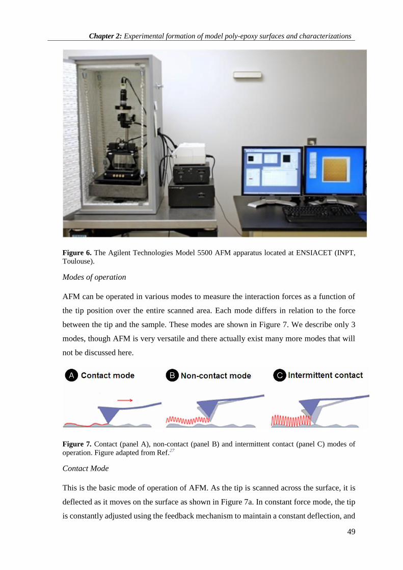
Chapter 2: Experimental formation of model poly-epoxy surfaces and characterizations
49
Figure 6. The Agilent Technologies Model 5500 AFM apparatus located at ENSIACET (INPT,
Toulouse).
Modes of operation
AFM can be operated in various modes to measure the interaction forces as a function of
the tip position over the entire scanned area. Each mode differs in relation to the force
between the tip and the sample. These modes are shown in Figure 7. We describe only 3
modes, though AFM is very versatile and there actually exist many more modes that will
not be discussed here.
Figure 7. Contact (panel A), non-contact (panel B) and intermittent contact (panel C) modes of
operation. Figure adapted from Ref.27
Contact Mode
This is the basic mode of operation of AFM. As the tip is scanned across the surface, it is
deflected as it moves on the surface as shown in Figure 7a. In constant force mode, the tip
is constantly adjusted using the feedback mechanism to maintain a constant deflection, and

Modelling the DGEBA-EDA poly-epoxy and its reactivity towards copper: experimental and
numerical approach
50
therefore constant height above the surface. The changes in the feedback signal required to
maintain the force constant are used to reconstruct the topography. As the tip is in hard
contact with the surface, the stiffness of the cantilever needs to be less than that of the
effective spring constant holding atoms together, which is on the order 1-10 nN/nm. Most
contact mode levers have a spring constant of <1 N/m so that soft materials are not
damaged.
In addition, a large class of materials (such as semiconductors and insulators), can trap
electrostatic charge. This charge can lead to additional attractive forces between the probe
and sample. All of these forces combine to define a minimum normal force that can be
controllably applied by the probe to the sample. This normal force creates a substantial
frictional force as the probe scans over the sample. It appears that these frictional forces
are far more destructive than the normal force and can damage the sample, the tip, and
corrupt the resulting data. An attempt to avoid this problem is the Non-contact Mode.
Non-contact mode
This mode relies on the use of an oscillating cantilever. A stiff cantilever oscillates in the
attractive regime, meaning that the tip is quite close to the sample, but not touching it as
shown in Figure 7b. The forces between the tip and the sample are quite low, in the order
of pN. The oscillation amplitude, phase and resonance frequency are modified by tip-
sample interaction forces. These changes in oscillation with respect to the forced reference
oscillation provide information about several properties of the samples. The detection is
based on measuring changes to the resonance frequency or amplitude of the cantilever.
Intermittent Contact Mode
In intermittent contact mode (a.k.a “Tapping ModeTM”) of operation, a stiff cantilever
oscillates closer to the sample than in non-contact mode. Part of the oscillation extends into
the repulsive regime, so the tip intermittently touches or “taps” the surface. Very stiff
cantilevers are typically used, as tips can get “stuck” in the water layer absorbed on the
sample surface, if any exists. The major advantage of tapping the surface is the improved
lateral resolution on soft samples. Typical Tapping ModeTM operation is carried out using
amplitude modulation detection with a lock-in amplifier. For the purposes of our project
we use the Contact and TappingTM modes for the analysis of the polymer surfaces.
Following in the next section are AFM results for the pristine poly-epoxy surface.
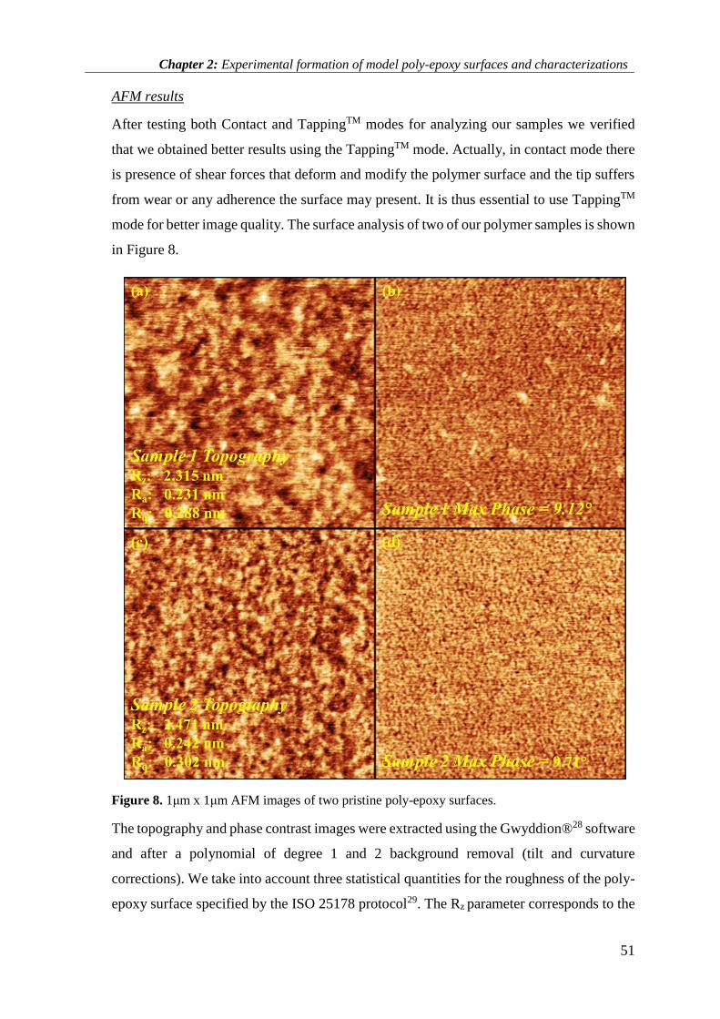
Chapter 2: Experimental formation of model poly-epoxy surfaces and characterizations
51
AFM results
After testing both Contact and TappingTM modes for analyzing our samples we verified
that we obtained better results using the TappingTM mode. Actually, in contact mode there
is presence of shear forces that deform and modify the polymer surface and the tip suffers
from wear or any adherence the surface may present. It is thus essential to use TappingTM
mode for better image quality. The surface analysis of two of our polymer samples is shown
in Figure 8.
Figure 8. 1μm x 1μm AFM images of two pristine poly-epoxy surfaces.
The topography and phase contrast images were extracted using the Gwyddion®28 software
and after a polynomial of degree 1 and 2 background removal (tilt and curvature
corrections). We take into account three statistical quantities for the roughness of the poly-
epoxy surface specified by the ISO 25178 protocol29. The Rz parameter corresponds to the

Modelling the DGEBA-EDA poly-epoxy and its reactivity towards copper: experimental and
numerical approach
52
height between the minimum and maximum points. The Ra parameter is the mean
arithmetical roughness which is the parameter we are more interested in having a <1nm
value as mentioned in Section 2.1. The Rq parameter is the root mean squared (RMS)
deviation of the surface profile. The Ra value of these 1μm x 1μm surface areas are 0.231
and 0.242 nm respectively. This roughness fulfills the criterion we set for the non-
metallized surface required to observe the first steps of growth of Cu clusters. Figures 8b
and 8d show the phase contrast imaging. Since the phase contrast remains below 10°, we
assess that the viscoelastic properties are constant over the micrometric surface area.
Therefore we assume that the surface is chemically homogeneous. We can also observe
that although the surface roughness is low there are some blobs and troughs of up to 2.5
nm-high/deep.
Introduction to X-Ray Photoelectron Spectroscopy
X-Ray Photoelectron Spectroscopy (XPS) is a surface analysis technique which allows the
determination of the elemental composition of a surface (from a few Å up to 10 nm-deep),
the contamination level, the local bonding of atoms, or the oxidation states. XPS is
achieved by irradiating a sample with soft X-Rays and by analyzing the energy of the
electrons emitted by the surface layer. When the photon source emits photons at a high-
enough frequency, then electrons of the core-level of atoms are ejected (and called
photoelectrons). The kinetic energy that remains on these photoelectrons carries intrinsic
information, such as the binding energy of the electron in its atomic core-level. Electrons
binding energies are element and bond specific, and thus identifications can be performed.
The equation in PES is given by Equation 5.
𝐵𝐸 = ℎ𝑣 − 𝐾𝐸 − 𝜑𝑠𝑎𝑚𝑝𝑙𝑒 (5)
where hν is the energy of the incident photon, KE is the kinetic energy of the emitted
electron, BE is the binding energy of the photo emitted electron, and φ is the work function
of the sample. Actually, since the sample and spectrometer are electrically connected, their
Fermi levels are equal.

Chapter 2: Experimental formation of model poly-epoxy surfaces and characterizations
53
Therefore, the photoelectrons are submitted to an electric field caused by the difference
(φsample – φspec) of both work functions. The complete equation now writes:
𝐵𝐸 = ℎ𝑣 − 𝐾𝐸 − 𝜑𝑠𝑎𝑚𝑝𝑙𝑒 + (𝜑𝑠𝑎𝑚𝑝𝑙𝑒 − 𝜑𝑠𝑝𝑒𝑐) = ℎ𝑣 − 𝐾𝐸 − 𝜑𝑠𝑝𝑒𝑐 (6)
𝜑𝑠𝑝𝑒𝑐 is a constant that is determined by calibration of a given apparatus.
Theoretically, the XPS process is described in a two-step model, with two distinct states
called the initial (before ionization) and the final (the pot-electron is in vacuum) states.
They are depicted in Figure 9. The initial state is the real state of the matter that we should
like to characterize, whereas the final state is an artefact that is intrinsically related to the
measurement principle. Unfortunately, the photoelectrons carry both initial and final state
contributions. Final states can have comprehensive effects on the XPS spectra. For
instance, the new core-level hole will be screened by surrounding electrons and thus modify
the electric field crossed by the photoelectron. Its kinetic energy will be affected, and so its
apparent binding energy. Consecutively, simulations of XPS spectra performed with initial
state calculations are likely to lead to fundamental discrepancies. We will show two
different calculation methods in Chapter 3 where final state effects are taken into account.
Figure 9. Principles of measurements in XPS adapted from Ref30.

Modelling the DGEBA-EDA poly-epoxy and its reactivity towards copper: experimental and
numerical approach
54
An X-Ray photoelectron spectrometer consists of the following components: (i) a vacuum
system that ensures a high or ultrahigh vacuum that is necessary to maximize the electrons
diffusion towards the detector, (ii) the X-Ray source, (iii) an electron-energy analyzer, and
(iv) a PC that both controls the spectrometer and processes the spectra. The apparatus we
use at our laboratory is the ThermoScientific XPS Kalpha as shown in Figure 10. It is
equipped with a monochromatic Al Kα source (hν = 1486.6 eV). At a pass energy of 30 eV
the FWHM is 0.7 eV on the Ag3d5/2 peak of a silver standard. The FWHM of the Ag peak
is commonly taken as providing an estimate of the experimental resolution of the XPS
spectra.
Figure 10. The Thermoscientific K-Alpha XPS aparatus (image provided by the vender's site).
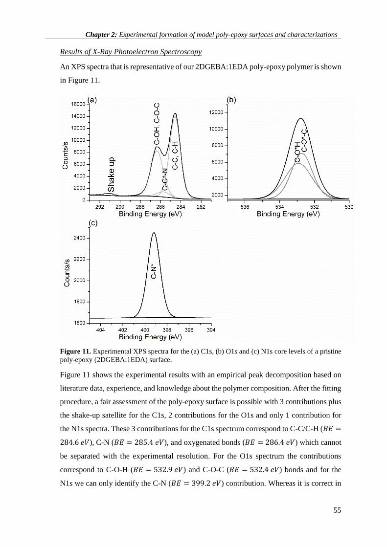
Chapter 2: Experimental formation of model poly-epoxy surfaces and characterizations
55
Results of X-Ray Photoelectron Spectroscopy
An XPS spectra that is representative of our 2DGEBA:1EDA poly-epoxy polymer is shown
in Figure 11.
Figure 11. Experimental XPS spectra for the (a) C1s, (b) O1s and (c) N1s core levels of a pristine
poly-epoxy (2DGEBA:1EDA) surface.
Figure 11 shows the experimental results with an empirical peak decomposition based on
literature data, experience, and knowledge about the polymer composition. After the fitting
procedure, a fair assessment of the poly-epoxy surface is possible with 3 contributions plus
the shake-up satellite for the C1s, 2 contributions for the O1s and only 1 contribution for
the N1s spectra. These 3 contributions for the C1s spectrum correspond to C-C/C-H (𝐵𝐸 =
284.6 𝑒𝑉), C-N (𝐵𝐸 = 285.4 𝑒𝑉), and oxygenated bonds (𝐵𝐸 = 286.4 𝑒𝑉) which cannot
be separated with the experimental resolution. For the O1s spectrum the contributions
correspond to C-O-H (𝐵𝐸 = 532.9 𝑒𝑉) and C-O-C (𝐵𝐸 = 532.4 𝑒𝑉) bonds and for the
N1s we can only identify the C-N (𝐵𝐸 = 399.2 𝑒𝑉) contribution. Whereas it is correct in
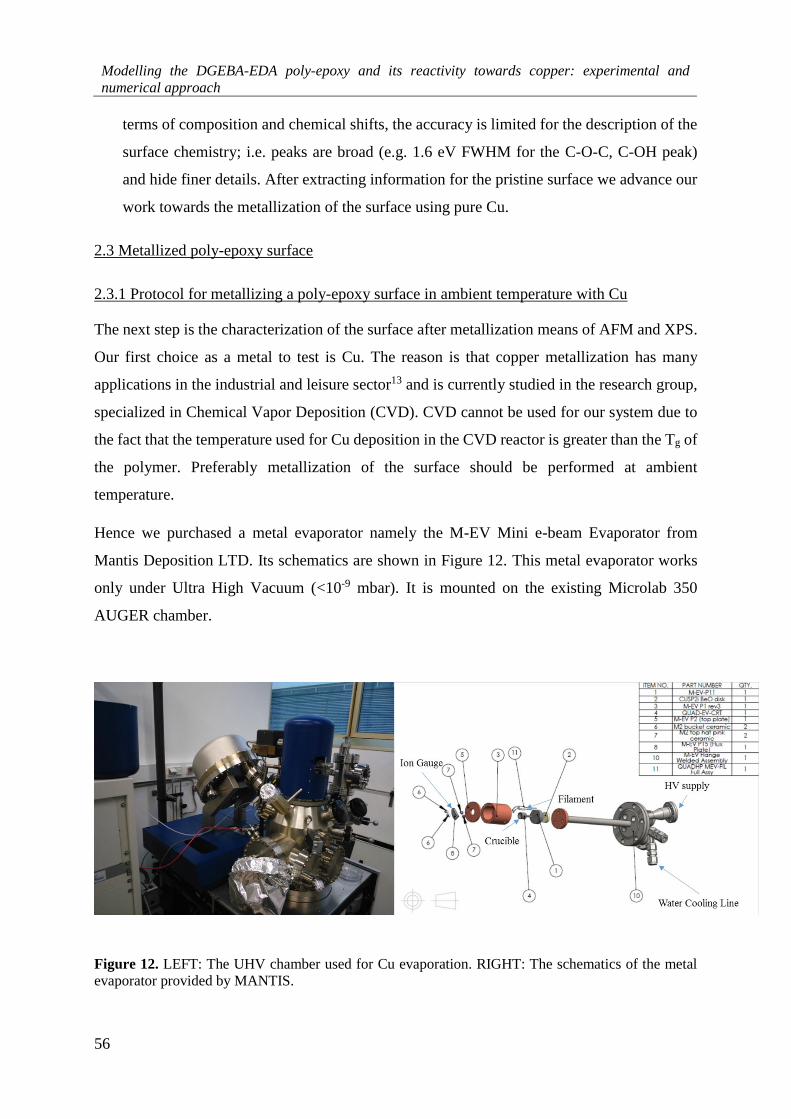
Modelling the DGEBA-EDA poly-epoxy and its reactivity towards copper: experimental and
numerical approach
56
terms of composition and chemical shifts, the accuracy is limited for the description of the
surface chemistry; i.e. peaks are broad (e.g. 1.6 eV FWHM for the C-O-C, C-OH peak)
and hide finer details. After extracting information for the pristine surface we advance our
work towards the metallization of the surface using pure Cu.
2.3 Metallized poly-epoxy surface
2.3.1 Protocol for metallizing a poly-epoxy surface in ambient temperature with Cu
The next step is the characterization of the surface after metallization means of AFM and XPS.
Our first choice as a metal to test is Cu. The reason is that copper metallization has many
applications in the industrial and leisure sector13 and is currently studied in the research group,
specialized in Chemical Vapor Deposition (CVD). CVD cannot be used for our system due to
the fact that the temperature used for Cu deposition in the CVD reactor is greater than the Tg of
the polymer. Preferably metallization of the surface should be performed at ambient
temperature.
Hence we purchased a metal evaporator namely the M-EV Mini e-beam Evaporator from
Mantis Deposition LTD. Its schematics are shown in Figure 12. This metal evaporator works
only under Ultra High Vacuum (<10-9 mbar). It is mounted on the existing Microlab 350
AUGER chamber.
Figure 12. LEFT: The UHV chamber used for Cu evaporation. RIGHT: The schematics of the metal
evaporator provided by MANTIS.

Chapter 2: Experimental formation of model poly-epoxy surfaces and characterizations
57
The protocol for the metallization involves the following steps:
Initial outgassing (of the empty source)
Melting the source material
Our source material is a 5N purity copper (99.999% pure, Goodfellow). The source material
must first be melted before the evaporation can take place, in order to complete the outgassing
of the bulk.
The power obtained at a given filament current will be dependent upon the gap and subsequent
field gradient between filament and evaporation source. We then construct a plot of power as a
function of the filament current in order to decide which is the ideal power setting for the
evaporation as shown in Figure 13.
Figure 13. Filament power as function of the current to determine the starting point for power for
evaporization of Cu
The initial power to start the evaporation is 25W corresponding to the inflexion of the curve.
This initial power corresponds to a flux of 23.2 nA. The metallization takes place under UHV
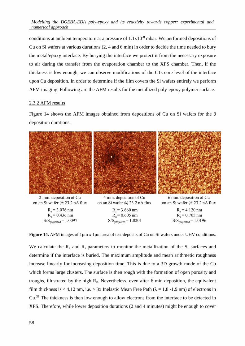
Modelling the DGEBA-EDA poly-epoxy and its reactivity towards copper: experimental and
numerical approach
58
conditions at ambient temperature at a pressure of 1.1x10⁻⁸ mbar. We performed depositions of
Cu on Si wafers at various durations (2, 4 and 6 min) in order to decide the time needed to bury
the metal/epoxy interface. By burying the interface we protect it from the necessary exposure
to air during the transfer from the evaporation chamber to the XPS chamber. Then, if the
thickness is low enough, we can observe modifications of the C1s core-level of the interface
upon Cu deposition. In order to determine if the film covers the Si wafers entirely we perform
AFM imaging. Following are the AFM results for the metallized poly-epoxy polymer surface.
2.3.2 AFM results
Figure 14 shows the AFM images obtained from depositions of Cu on Si wafers for the 3
deposition durations.
Figure 14. AFM images of 1μm x 1μm area of test deposits of Cu on Si wafers under UHV conditions.
We calculate the Rz and Ra parameters to monitor the metallization of the Si surfaces and
determine if the interface is buried. The maximum amplitude and mean arithmetic roughness
increase linearly for increasing deposition time. This is due to a 3D growth mode of the Cu
which forms large clusters. The surface is then rough with the formation of open porosity and
troughs, illustrated by the high Rz. Nevertheless, even after 6 min deposition, the equivalent
film thickness is < 4.12 nm, i.e. > 3x Inelastic Mean Free Path (λ = 1.8 -1.9 nm) of electrons in
Cu.31 The thickness is then low enough to allow electrons from the interface to be detected in
XPS. Therefore, while lower deposition durations (2 and 4 minutes) might be enough to cover

Chapter 2: Experimental formation of model poly-epoxy surfaces and characterizations
59
the surface, we conservatively choose the 6 min deposits for XPS. The poly-epoxy surface is
then metallized and AFM imaging is performed. The results for the Cu covered surface are
shown in Figure 15.
Figure 15. AFM results for a poly-epoxy surface fully covered with Cu.
The maximum amplitude is 6 nm. The 3D growth mode of the Cu on the poly-epoxy surface
is significantly different from the 3D growth on the Si wafer. Due to the difference in
nucleation density, the Ra of the Cu films on the poly-epoxy surface is larger than that on
the Si wafer surface. That is an effect of the low reactivity of the poly-epoxy surface that
doesn’t promote Cu/epoxy interactions to the benefit of Cu/Cu interactions and thus create
less number of nuclei/nm2.
2.3.3 XPS results
Figure 16 shows the comparison between the C1s XPS spectra of the pristine and the
metallized poly-epoxy surface. It must be noted that for XPS, we should complete the
analysis with the Auger peaks of Cu that may demonstrate Cu oxidation. But, since the
metallic Cu contribution is in large excess compared to the Cu contribution of the interface,
no features are found in the Cu LMM spectrum that would differ from a bulk Cu.
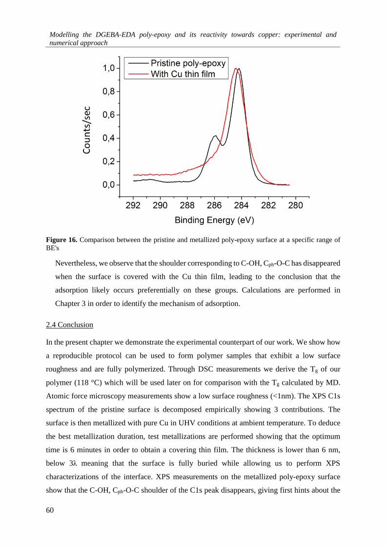
Modelling the DGEBA-EDA poly-epoxy and its reactivity towards copper: experimental and
numerical approach
60
Figure 16. Comparison between the pristine and metallized poly-epoxy surface at a specific range of
BE's
Nevertheless, we observe that the shoulder corresponding to C-OH, Cph-O-C has disappeared
when the surface is covered with the Cu thin film, leading to the conclusion that the
adsorption likely occurs preferentially on these groups. Calculations are performed in
Chapter 3 in order to identify the mechanism of adsorption.
2.4 Conclusion
In the present chapter we demonstrate the experimental counterpart of our work. We show how
a reproducible protocol can be used to form polymer samples that exhibit a low surface
roughness and are fully polymerized. Through DSC measurements we derive the Tg of our
polymer (118 °C) which will be used later on for comparison with the Tg calculated by MD.
Atomic force microscopy measurements show a low surface roughness (<1nm). The XPS C1s
spectrum of the pristine surface is decomposed empirically showing 3 contributions. The
surface is then metallized with pure Cu in UHV conditions at ambient temperature. To deduce
the best metallization duration, test metallizations are performed showing that the optimum
time is 6 minutes in order to obtain a covering thin film. The thickness is lower than 6 nm,
below 3λ meaning that the surface is fully buried while allowing us to perform XPS
characterizations of the interface. XPS measurements on the metallized poly-epoxy surface
show that the C-OH, Cph-O-C shoulder of the C1s peak disappears, giving first hints about the
Chapter 2: Experimental formation of model poly-epoxy surfaces and characterizations
61
Cu adsorption mechanism. This study is deepened in Chapter 3 where we will demonstrate how
different approaches in quantum calculations can be used to gain better understanding on the
XPS spectra of the pristine and metallized surfaces.
Bibliography
1. Aerospace materials — past, present, and future - Aerospace Manufacturing and Design. Available
at: http://www.aerospacemanufacturinganddesign.com/article/amd0814-materials-aerospace-
manufacturing/. (Accessed: 25th September 2017)
2. Flosbach, C. & Fugier, R. Epoxy Functional Acrylic Polymers for High Performance Coating
Applications. in Epoxy Polymers (eds. Pascault, J.-P. & Williams, R. J. J.) 39–54 (Wiley-VCH
Verlag GmbH & Co. KGaA, 2010). doi:10.1002/9783527628704.ch3
3. Gandini, A. Epoxy Polymers Based on Renewable Resources. in Epoxy Polymers (eds. Pascault, J.-
P. & Williams, R. J. J.) 55–78 (Wiley-VCH Verlag GmbH & Co. KGaA, 2010).
doi:10.1002/9783527628704.ch4
4. Chandrasekhar, P. et al. Conducting Polymer (CP) infrared electrochromics in spacecraft thermal
control and military applications. in Synthetic metals 135–36, 23–24 (Elsevier, 2003).
5. Feldman, D. & Barbalata, A. Synthetic Polymers: Technology, Properties, Applications. (Springer
Netherlands, 1996).
6. Zaporojtchenko, V. et al. Formation of metal–polymer interfaces by metal evaporation: influence
of deposition parameters and defects. Microelectron. Eng. 50, 465–471 (2000).
7. Ho, P. S. et al. Chemical bonding and reaction at metal/polymer interfaces. J. Vac. Sci. Technol.
Vac. Surf. Films 3, 739–745 (1985).
8. Burrell, M. C. et al. Characterization of Surface Modifications during Metallization of
Polyetherimide. in Metallized Plastics 1 223–233 (Springer, Boston, MA, 1989). doi:10.1007/978-
1-4899-0879-7_15
9. Bébin, P. & Prud’homme, R. E. Comparative XPS Study of Copper, Nickel, and Aluminum
Coatings on Polymer Surfaces. Chem. Mater. 15, 965–973 (2003).
10. Zaporojtchenko, V., Behnke, K., Thran, A., Strunskus, T. & Faupel, F. Condensation coefficients
and initial stages of growth for noble metals deposited onto chemically different polymer surfaces.
Appl. Surf. Sci. 144, 355–359 (1999).
11. Bou, M., Martin, J. M., Le Mogne, T. & Vovelle, L. Chemistry of the interface between aluminium
and polyethyleneterephthalate by XPS. Appl. Surf. Sci. 47, 149–161 (1991).
12. Wagner, A. J., Wolfe, G. M. & Fairbrother, D. H. Reactivity of vapor-deposited metal atoms with
nitrogen-containing polymers and organic surfaces studied by in situ XPS. Appl. Surf. Sci. 219,
317–328 (2003).
13. E. Sacher (ed.). Metallization of Polymers 2. (Plenum Publishers, 2002).
14. Travaly, Y., Bertrand, P., Rignanese, G.-M. & Gonze, X. Theoretical Modeling of the Nucleation
and Growth of Aluminium Films Thermally Evaporated onto Poly(ethylene terephthalate)
Substrate. J. Adhes. 66, 339–355 (1998).
15. Friedrich, J. F., Koprinarov, I., Giebler, R., Lippitz, A. & Unger, W. E. S. Reactions and
Intermediates at the Metal-Polymer Interface as Observed by XPS and NEXAFS Spectroscopy. J.
Adhes. 71, 297–321 (1999).
16. Wolany, D. et al. Combined ToF-SIMS/XPS study of plasma modification and metallization of
polyimide. Surf. Interface Anal. 27, 609–617 (1999).
17. Rastomjee, C. S. et al. Aluminium metallisation of argon and oxygen plasma-modified
polycarbonate thin film surfaces. Appl. Surf. Sci. 136, 280–297 (1998).
18. Kanzow, J. et al. Formation of a metal/epoxy resin interface. Appl. Surf. Sci. 239, 227–236 (2005).
19. Infrared Spectroscopy - Materials Science, Engineering and Technology. Available at:
https://www.intechopen.com/books/infrared-spectroscopy-materials-science-engineering-and-
technology. (Accessed: 26th September 2017)
20. Nikolic, G. et al. Fast Fourier Transform IR Characterization of Epoxy GY Systems Crosslinked
with Aliphatic and Cycloaliphatic EH Polyamine Adducts. Sensors 10, 684–696 (2010).

Modelling the DGEBA-EDA poly-epoxy and its reactivity towards copper: experimental and
numerical approach
62
21. Duguet, T. et al. Toward a computational and experimental model of a poly-epoxy surface. Appl.
Surf. Sci. 324, 605–611 (2015).
22. Bessaguet, C. Synthèse de polymères thermodurcissables modèles et caractérisation de leur surface
par XPS et AFM, Rapport de stage Master 2. (Institut National Polytechnique de Toulouse, 2013).
23. Bliznyuk, V. N., Assender, H. E. & Briggs, G. A. D. Surface Glass Transition Temperature of
Amorphous Polymers. A New Insight with SFM. Macromolecules 35, 6613–6622 (2002).
24. Bermejo, J. S. & Ugarte, C. M. Influence of Cross-Linking Density on the Glass Transition and
Structure of Chemically Cross-Linked PVA: A Molecular Dynamics Study. Macromol. Theory
Simul. 18, 317–327 (2009).
25. Marti, O., Stifter, T., Waschipky, H., Quintus, M. & Hild, S. Scanning probe microscopy of
heterogeneous polymers. Colloids Surf. Physicochem. Eng. Asp. 154, 65–73 (1999).
26. Tsui, O. K. C., Wang, X. P., Ho, J. Y. L., Ng, T. K. & Xiao, X. Studying Surface Glass-to-Rubber
Transition Using Atomic Force Microscopic Adhesion Measurements. Macromolecules 33, 4198–
4204 (2000).
27. Funes, D. 2.2. Atomic force microscope (AFM).
28. Nečas, D. & Klapetek, P. Gwyddion: an open-source software for SPM data analysis. Cent. Eur. J.
Phys. 10, 181–188 (2012).
29. ISO 25178-2:2012 - Geometrical product specifications (GPS) -- Surface texture: Areal -- Part 2:
Terms, definitions and surface texture parameters. Available at:
https://www.iso.org/standard/42785.html. (Accessed: 15th October 2017)
30. XPS Summary (Sylvia Natividad, Arena Holguin, and Gabriel Gonzalez) - Sylvia Natividad -
Confluence. Available at: https://wiki.utep.edu/pages/viewpage.action?pageId=51217510.
(Accessed: 15th October 2017)
31. Powell, C. J. & Jablonski, A. NIST Electron Inelastic-Mean-Free-Path Database - Version 1.2,
National Institute of Standards and Technology, Gaithersburg, MD. (2010).

Chapter 3: HF and DFT computations for the simulation of XPS spectra
63
Chapter 3: HF and DFT computations for the simulation of XPS
spectra
3.1 Introduction
Our goal is to create numerical models of the poly-epoxy surface. In this chapter and in the next
one, we propose two models, each one adapted to part of our studies. As it will be explained in
the perspectives of the manuscript, the proposal of an integrated model will be the next
objective, beyond this PhD work.
The first model that we study is a molecular model: one DGEBA molecule connected to one
EDA molecule. This model, called the ‘dimer model’ in the following, is used to simulate the
XPS spectra for the pristine surface. Thanks to these results, we are able to analyze the
experimental spectrum more accurately than with the exclusive use of experiments and
literature. This dimer model is also used to study the mechanism of the metallization process
with copper by the determination of Cu adsorption energies on the dimer. The most stable
adsorption sites can then be determined and XPS spectra of the molecular model of the
metallized surface are simulated and compared with the experimental counterpart.
3.2 General introduction to XPS
As explained in Chapter 2, in X-Ray Photoelectron Spectroscopy (XPS), photons emitted by a
monochromatic source (photons of fixed energy ℎ𝑣) are absorbed by an atom and this can lead
to the emission of an electron and the ionization of the atom. With XPS, core-levels are analyzed
(while ultraviolet photoelectron spectroscopy (UPS) probes valence levels).
The kinetic energy distribution of the emitted photoelectrons is therefore measured by an
electron energy analyzer. The binding energy of the photoelectron in the atom is then given by
Equation 1:
𝐵𝐸𝑘 = ℎ𝑣 − 𝐾𝐸 − 𝜑𝑠𝑝𝑒𝑐 (1)
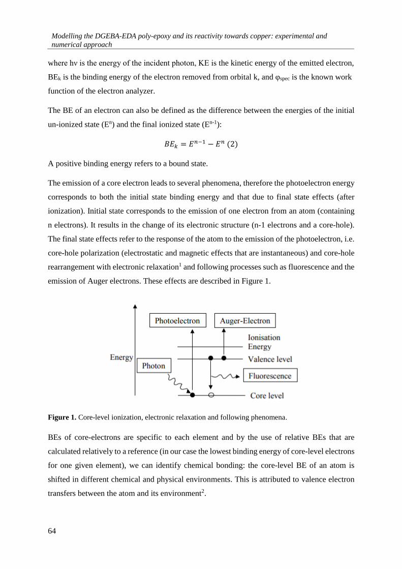
Modelling the DGEBA-EDA poly-epoxy and its reactivity towards copper: experimental and
numerical approach
64
where hν is the energy of the incident photon, KE is the kinetic energy of the emitted electron,
BEk is the binding energy of the electron removed from orbital k, and φspec is the known work
function of the electron analyzer.
The BE of an electron can also be defined as the difference between the energies of the initial
un-ionized state (En) and the final ionized state (En-1):
𝐵𝐸𝑘 = 𝐸𝑛−1 − 𝐸𝑛 (2)
A positive binding energy refers to a bound state.
The emission of a core electron leads to several phenomena, therefore the photoelectron energy
corresponds to both the initial state binding energy and that due to final state effects (after
ionization). Initial state corresponds to the emission of one electron from an atom (containing
n electrons). It results in the change of its electronic structure (n-1 electrons and a core-hole).
The final state effects refer to the response of the atom to the emission of the photoelectron, i.e.
core-hole polarization (electrostatic and magnetic effects that are instantaneous) and core-hole
rearrangement with electronic relaxation1 and following processes such as fluorescence and the
emission of Auger electrons. These effects are described in Figure 1.
Figure 1. Core-level ionization, electronic relaxation and following phenomena.
BEs of core-electrons are specific to each element and by the use of relative BEs that are
calculated relatively to a reference (in our case the lowest binding energy of core-level electrons
for one given element), we can identify chemical bonding: the core-level BE of an atom is
shifted in different chemical and physical environments. This is attributed to valence electron
transfers between the atom and its environment2.
Chapter 3: HF and DFT computations for the simulation of XPS spectra
65
In an experimental XPS spectrum, peaks can be decomposed into several components if a given
element is found in different bonds and environment. We showed in chapter 2 that this can be
achieved thanks to the literature and to rigorous databases. But quantum calculations can help
for an even more accurate interpretation of the spectra. Simulations of XPS spectra can be done
at several levels of theory: (i) at the Hartree-Fock level of theory with the use of the Koopmans’
theorem3 and the ΔSCF theory4 , (ii) and in the framework of the density functional theory using
the Generalized Transition State theory (GTS)5. We present now the main methodologies for
the calculation of XPS spectra.
3.3 Calculation of XPS spectra
3.3.1 Hartree-Fock calculations
At the simplest level, Koopmans’ theorem3 provides a straightforward method to make a rough
evaluation of the valence and core binding energies. Koopmans’s theorem states that “the
negative of the eigenvalue of an occupied orbital from a Hartree-Fock calculation is equal to
the vertical ionization energy to the ion state formed by removal of one electron from that
orbital, provided the distributions of the remaining electrons do not change”. Thus BEs can be
calculated by:
𝐵𝐸𝑘 = −휀𝑘 (3)
where 휀𝑘 is a molecular orbital energy resulting from a Hartree-Fock calculation on the neutral
parent molecule.
This method gives results that shift away from the experimental values (up to a difference of
10-20 eV)6 because it does not take into account final state effects.
Various alternatives can be used to compute core-electron BEs. One is the HF-ΔSCF method
that includes the initial state contributions due to the charge distribution in the ground state and
the final state contributions due to the electronic relaxation in response to the core-hole. In the
ΔSCF method, the BEs are taken as the difference in the HF Self-consistent field, SCF, energies
of the ground state (𝐸𝑆𝐶𝐹𝑛 ) and the core-ionized state (𝐸𝑆𝐶𝐹
𝑛−1)7:
𝐵𝐸𝑘 = ∆𝐸 = 𝐸𝑆𝐶𝐹𝑛−1 − 𝐸𝑆𝐶𝐹
𝑛 (4)
It is necessary to include the final state effects since the electronic relaxation may be different
for the ionization of different inequivalent atoms8. The quality of the results then depends on
the theoretical treatment used in both SCF calculations but the accuracy of the HF-ΔSCF

Modelling the DGEBA-EDA poly-epoxy and its reactivity towards copper: experimental and
numerical approach
66
method was adequate for our purposes. This adequacy has been documented in the review of
Ref.7 and in three recent papers8–10 where the XPS BEs have been studied for a large number
of molecules containing C, N, and O atoms.
An advantage of using HF wavefunctions is that they provide a way to determine the relative
intensities, Irel, of the main peaks. In our calculations, the XPS intensities for these main peaks
were determined on the basis of the Sudden Approximation, SA11. The SA is based on several
assumptions:
- The final state wavefunction of the system (containing n electrons) after ionization can
be expressed as an anti-symmetrized product of one wavefunction including (n-1)
electrons 𝛹𝑘𝑛−1 and a one electron continuum orbital
- At the time of the photoionization, 𝛹𝑘𝑛−1 is given “by suddenly removing one electron”7
to the orbital number k without allowing any electronic relaxation. This wavefunction,
called a frozen orbital (FO) wavefunction, is thus determined from the orbitals that were
calculated for the neutral molecule ground state.
This 𝛹𝑘𝑛−1 wavefunction is not solution of the (n-1) electron Hamiltonian 𝐻𝑛−1. To compute
energies, 𝛹𝑘𝑛−1 needs thus to be expressed from (n-1) electron wavefunctions that are
eigenfunctions of 𝐻𝑛−1 :
𝐻𝑛−1 𝛹𝛼𝑛−1 = 𝐸𝛼
𝑛−1 𝛹𝛼𝑛−1 (5)
𝛹𝑘𝑛−1 = ∑ 𝐶𝑘,𝛼
𝛼
𝛹𝛼𝑛−1 (6)
For a peak corresponding to the ionized molecule wavefunction 𝛹𝛼𝑛−1, the relative intensity is
the probability for the system to be in this state:
𝐼𝑟𝑒𝑙(𝑘, 𝛼) = |⟨ 𝛹𝑘𝑛−1| 𝛹𝛼
𝑛−1⟩|2(7)
This is the square of the overlap of the (n-1) electron FO wavefunction with the ∆SCF
wavefunction where the removed C1s electron has been fully screened.
Since the orbitals of the set optimized for the hole-states are not orthogonal to the orbitals of
the set optimized for the ground state, GS, it is necessary to use a sum over overlap integrals
times a minor of the overlap determinant between the GS and the core-hole orbitals.12

Chapter 3: HF and DFT computations for the simulation of XPS spectra
67
3.3.2 Density Functional Theory calculations
In the framework of the density functional theory, final state effects have also to be taken into
account to accurately simulate XPS spectra. Methods developed to include initial and final state
effects are based on the Slater’s transition-state (TS)13, first generalized by Williams et al5, and
later slightly modified by Chong et al14,15. This latter development is known as the unrestricted
Generalized Transition State theory (uGTS). The idea, based on the Taylor series expansion of
the energy in terms of the shell occupation, is to remove a fraction of electron from the
molecular orbital of interest.
The aim of Slater’s transition state is the accurate evaluation of electronic excitation energies
of finite molecular systems. The excitation energy 𝛥𝐸 is defined as the difference in the total
energy of the electronic system in study before and after excitation:
𝛥𝐸 = 𝐸𝑓𝑖𝑛𝑎𝑙 − 𝐸𝑖𝑛𝑖𝑡𝑖𝑎𝑙 (8)
The transition state concept was combined with an expression of the total energy of the system
as an analytic function of the occupation numbers ni of orbitals {𝜓𝑖(𝑟)}:
𝐸 = 𝐸(𝑛1, 𝑛2, … , 𝑛𝑖) (9)
And then, it could be used to determine ionization energies, for instance core-ionization
energies:
𝛥𝐸 = 𝐸𝑓𝑖𝑛𝑎𝑙 − 𝐸𝑖𝑛𝑖𝑡𝑖𝑎𝑙 = 𝐸(0,1,1, … ,1) − 𝐸(1,1,1, … ,1) (10)
The analytic expression of the total energies allows their Taylor series expansion. If both the
initial energy 𝐸𝑖𝑛𝑖𝑡𝑖𝑎𝑙 and final energy 𝐸𝑓𝑖𝑛𝑎𝑙 are expanded about the common point in n space
{𝑛𝑖} defined below:
{𝑛𝑖} = (1
2, 1,1, … ,1) (11)
then, all the even order terms in the expansion in powers of 𝛿𝑛1 are zero and finally it can be
written:
∆𝐸 =𝜕𝐸
𝜕𝑛1+ 𝑡𝑒𝑟𝑚𝑠 𝑜𝑓 𝑜𝑟𝑑𝑒𝑟 (𝛿𝑛1)3 (12)
In the Slater's transition state method, only the first term in Equation 12 is kept and 𝑛1 =1
2.
Modelling the DGEBA-EDA poly-epoxy and its reactivity towards copper: experimental and
numerical approach
68
Moreover, using the Janak’s16 theorem, 𝜕𝐸
𝜕𝑛1 is equal to the opposite of the energy ε1 of the orbital
number 1 with the occupation number n1. Then:
∆𝐸 = −휀1 (1
2) (13)
Later Williams et al.5 demonstrated that the core-ionization energy can be more accurately
calculated as:
ΔΕ = −1
4 휀𝑘(1) −
3
4휀𝑘 (
1
3) (14)
Chong14,15 and Endo et al.6, 19–21 later demonstrated that the most accurate results are obtained
when the calculation with an occupation number of 1
3 is performed as an unrestricted
computation. We now present the results of our studies using both HF-ΔSCF and DFT-uGTS
methodologies.
3.4 Poly-epoxy pristine polymer surface
In Chapter 2, we presented an experimental XPS spectrum for the pristine poly-epoxy surface.
The analysis of the experimental spectrum, obtained by the exclusive use of experiments and
literature, was good but could be more accurate thanks to simulations of the XPS spectrum of
the polymer by quantum calculations. We present now the results of our simulations.
We first optimized the geometry of the dimer model with DFT calculations. The optimized
geometry was then used to simulate the XPS spectrum of the pristine surface at the Hartree-
Fock level of theory. In a second time, we performed additional DFT computations to simulate
the XPS spectra of the pristine and metallized surfaces in the uGTS framework.
3.4.1 Geometry Optimization Calculations
The first step consists to determine the most stable geometry for the monomer (DGEBA), the
cross-linker (EDA) and the dimer shown in Figures 2 and 3 respectively.
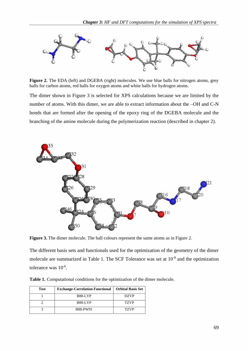
Chapter 3: HF and DFT computations for the simulation of XPS spectra
69
Figure 2. The EDA (left) and DGEBA (right) molecules. We use blue balls for nitrogen atoms, grey
balls for carbon atoms, red balls for oxygen atoms and white balls for hydrogen atoms.
The dimer shown in Figure 3 is selected for XPS calculations because we are limited by the
number of atoms. With this dimer, we are able to extract information about the –OH and C-N
bonds that are formed after the opening of the epoxy ring of the DGEBA molecule and the
branching of the amine molecule during the polymerization reaction (described in chapter 2).
Figure 3. The dimer molecule. The ball colours represent the same atoms as in Figure 2.
The different basis sets and functionals used for the optimization of the geometry of the dimer
molecule are summarized in Table 1. The SCF Tolerance was set at 10-8 and the optimization
tolerance was 10-6.
Table 1. Computational conditions for the optimization of the dimer molecule.
Test Exchange-Correlation Functional Orbital Basis Set
1 B88-LYP DZVP
2 B88-LYP TZVP
3 B88-PW91 TZVP

Modelling the DGEBA-EDA poly-epoxy and its reactivity towards copper: experimental and
numerical approach
70
The orbital basis sets that are chosen for comparison are the double zeta polarization basis set
(DZVP) and the triple zeta polarization (TZVP) basis set21,22. By using a polarization basis set
we take into account the fact that as atoms are brought closer, their charge distribution causes
a polarization effect (the positive charge is drawn to one side while the negative charge is drawn
to the other) which distorts the shape of the atomic orbitals, making our calculations more
accurate. We compare the optimized structures of the dimer molecule in the different
computational conditions. The results are given in Annex C. We conclude that for all the
functional/basis set combinations, the calculated bond lengths are in good agreement with
experimental values. Taking into account studies23,24 on the functional dependence of calculated
core energies, we decide for a better accuracy to choose the B88-PW91/TZVP optimized
geometry for the XPS HF simulations.
Concerning the other parameters for the DFT optimization, we tried to optimize the geometry
of the dimer using auxiliary basis sets to save computational time. Unfortunately when very
high optimization tolerances were chosen (e.g. 1x10-06), no convergence was achieved. Tests
also showed no significant difference in results by variation of the grid from FINE to EXTRA
FINE, so the use of an ADAPTIVE FINE grid was decided. An ADAPTIVE FINE grid means
that more points are taken into account when calculating various properties and thus accounts
for a larger sampling of the 3D space. To have a great accuracy in results the tolerance of the
grid was raised to 10-9 μHartree25. We used a value of 0.1 (scalar quantity) for the mixing
parameter that regulates the Hartree damping26 of the coefficients that determine the fitting of
the charge density.
3.4.2 XPS calculations using Hartree-Fock theory
We first chose the Hartree Fock level of theory and initiated a close collaboration with Prof.
Paul Bagus at the North Texas University. He performed all the calculations of the XPS hole-
states (ΔSCF method) and SA intensities on the dimer model using the CLIPS program.27
The HF energies of the ground state (GS) and the core-ionized state7 are calculated with a
modest basis set that is slightly more extended than double zeta, DZ+28. The basis set is made
with contracted Cartesian Gaussian functions. For the C, N, and O atoms, the basis set is based
on the 9s and 5p basis set of van Djinevelt29 contracted to 4s and 3p functions, (9,5/4,3). For
the H atoms, the basis set is (4,1/2,1) where the s basis function exponents are taken from van
Djineveldt29 supplemented by a p function with exponent 1.0. Calculations of Hartree-Fock

Chapter 3: HF and DFT computations for the simulation of XPS spectra
71
wavefunctions are performed for the ground state of the molecule and for configurations where
the 1s shell of each of the C atoms was singly occupied. Convergence to the hole-states where
the singly occupied orbital had the proper localized 1s character is ensured by selecting the
occupied orbitals at each SCF iteration according to a criterion of maximum overlap with the
starting guess for that iteration.30 However with an overlap criterion for selecting occupied
orbitals, there is a danger of converging to an excited state, especially if the changes from the
initial trial guess are large. When this occurs, it is necessary to change the order of the occupied
and virtual orbitals, perhaps in several steps, until one converges to the lowest energy state for
the core-hole configuration. This is an arduous manual procedure. A procedure to avoid this
manual effort is implemented to insure automatic convergence to the desired state. In the spirit
of Jolly’s equivalent core approximation31, the C atom to be core ionized is replaced with a N
atom and we determine the HF ground state orbitals for the closed shell positive ions for this
equivalent core molecule where it is not necessary to use the overlap criterion to select the
occupied orbitals. For the calculations on this equivalent core molecule, the same basis set as
for the real molecule of interest is used so that the orbitals for the fictitious molecule can be
used as the initial trial functions for the calculations on the core-hole state of the real molecule.
For these latter calculations, it is only necessary to specify that the 1s orbital centered on the
equivalent core atom is singly occupied. Since the equivalent core orbitals are a good
approximation to the orbitals of the lowest core-hole state,30 there is no difficulty in converging
to the desired state without manual intervention except for the preparation of the input files.
The left frame of Table 2 shows results obtained from the ΔSCF calculations. C1s orbitals can
be identified from the atom numbering of the first column derived from the model dimer shown
in Figure 3. Chemical shifts (ΔBEs) are all obtained from the orbital with the lowest energy
(C6), fixed at 0 eV. The third column shows the theoretical intensities calculated in the
framework of the SA. The relative SA intensities range between 0.65 and 0.75 meaning that,
depending on the C atom, 25% to 35% of the XPS intensity is lost from the main peak to shake
satellites. These data are used to build the theoretical C1s spectrum by computing a Voigt
convolution for each individual contribution. The Voigt convolution consists in the convolution
of a Gaussian and a Lorentzian function32, with full-width at half maximum (FWHM) of 0.9
eV and 0.1 eV33,34, respectively. The spectrum envelope is the sum of all contributions.

Modelling the DGEBA-EDA poly-epoxy and its reactivity towards copper: experimental and
numerical approach
72
Table 2. LEFT: Calculated chemical shift (ΔBE) and intensities for each orbitals of the dimer molecule
shown in Figure 1. CENTER: Functional group identification (the orbital of interest belong to atoms
marked with a *). RIGHT: The number and relative concentration of C1s orbitals in the solid poly-epoxy
from the stoichiometric ratio 2DGEBA:1EDA. Greyed rows correspond to orbitals which are present in
the model dimer, but no longer present in the fully-polymerized solid.
Model dimer Poly-epoxy (2 DGEBA + 1 EDA)
Orbitals ID ΔBE(ΔSCF)
(eV)
Calculated
relative intensity Functional groups
Number of
C1s orbitals Relative composition
C6 0,00 0,68 Cph*-Cquater 2 9,1%
C25 0,03 0,68 Cph*-Cquater 2
C2 0,04 0,67 Cph 2
36,4%
C29 0,08 0,68 Cph 2
C5 0,14 0,67 Cph 2
C30 0,16 0,67 Cph 2
C4 0,22 0,68 Cph 2
C26 0,24 0,67 Cph 2
C3 0,25 0,68 Cph 2
C27 0,25 0,68 Cph 2
C50 0,26 0,74 CH3 2 9,1%
C46 0,28 0,74 CH3 2
C24 0,82 0,74 Cquater 2 4,5%
C18 1,00 0,75 N-C-C*-N 2* 4,5%
C20 1,20 0,75 N(H2)-C*-C-N 0 n/a
C16 1,25 0,75 N-C*-C(OH) 4 9,1%
C1 1,89 0,65 Cph*-O-C 2 9,1%
C28 1,92 0,65 Cph*-O-C 2
C9 2,09 0,74 C-OH 4 9,1%
C8 2,36 0,73 C*-O-Cph 4 9,1%
C34 2,58 0,73 epoxy 0 n/a
C33 2,59 0,73 epoxy 0 n/a
C32 2,65 0,74 epoxy-C*-O-Cph 0 n/a
Figure 4a shows the experimental result, presented in chapter 2, with an empirical peak
decomposition based on literature data, experience, and knowledge about the polymer
composition. After the fitting procedure, a fair assessment of the poly-epoxy surface is possible
with 3 contributions plus the shake-up satellite, only. ΔBE (ΔSCF) and SA results are presented

Chapter 3: HF and DFT computations for the simulation of XPS spectra
73
in Figure 4b with the comparison of the experimental (grey full line) and simulated (black full
line) spectra. It helps distinguishing 9 contributions instead of 3 as the “empirical case”, hence
it provides more information than is obtained from the imperfect resolution of the XPS
experimental data. In this Figure 4b, a Tougaard background35 is subtracted from the
experimental spectrum and the simulated spectrum is positioned by applying a rigid shift until
the maximum intensity matches the maximum experimental intensity (normalized to 1.0). The
agreement between the experiment and the theory is rather good. The most serious limitation is
that the theoretical energy of the second peak at approx. 2.3 eV is too high with respect to
experiment by 0.3 eV. The intensity of this peak is also too low by 25%. Finally, there is a
difference at the leading, low BE edge of the spectra.
Figure 4. (a) Experimental C1s spectrum decomposed empirically. (b) Comparison of the experimental
(grey full line) and simulated (black full line) C1s spectra obtained from the sum of the calculated
contributions of each orbitals.
The identification of the bond responsible of the chemical shift of the atomic orbitals BE’s is
shown in the central column of Table 2. Some mixing was present for the C1s orbitals in the
initial, GS, state calculations where some of these orbitals were not localized exclusively on a

Modelling the DGEBA-EDA poly-epoxy and its reactivity towards copper: experimental and
numerical approach
74
single C atom but were distributed over a few of the C atoms; this occurred especially when the
C1s orbital energies were nearly degenerate. However, the singly occupied C1s orbitals of the
ionic state HF wavefunctions were all localized on a single C atom. The fact that the initial state
C1s orbitals were sometimes not localized was taken into account in our calculation of the SA
relative XPS intensities. Nine different environments can be identified from the data in Table 2
and the model molecule (the relevant C atom orbital is marked with a *), with the following
method.
1. Cph*-Cquater: C6 and C25 of the phenyl ring bonded to the unique quaternary carbon, C24.
2. Cph: C atoms of the 2 phenyl rings (C2-5, C26, C27, C29, and C30).
3. CH3: C46, C50.
4. Cquater: quaternary C (C24).
5. N-C-C*-N: C-N bond within the EDA molecule (C18). C20 is discarded because it is
bonded to a primary N(H2) which shifted its 1s electron BE by +0.2 eV as compared to
C18, whereas it is absent of the real surface. As a consequence C18 is counted twice
(C18 + “actual” C20).
6. N-C*-C(OH): C-N bond of the DGEBA molecule (C16) somehow shifted by the
neighboring C-OH.
7. Cph*-O-C: C atoms of the phenyl rings (C1 and C28) bonded to O (O7 and O31).
8. C-OH: C9.
9. C*-O-Cph: C atom from the DGEBA chain (C8). C32 is discarded because the
neighboring epoxy ring shifts its 1s electron BE by 0.29 eV as compared to C8, whereas
it is absent of the actual surface.

Chapter 3: HF and DFT computations for the simulation of XPS spectra
75
Therefore a first consequence of using theoretical modeling is that it offers the possibility to
decompose the XPS spectra with many contributions that are guaranteed by the theory. In that
sense the 3 broad contributions of Figure 4a now decompose into:
- C-C, C-H → phenyls C (ΔBE = +0‒0.25 eV) + CH3 (ΔBE = +0.26‒0.28 eV)).
- C-C*-N → C-C*-N within EDA (ΔBE = +1.00 eV), C-C*-N within DGEBA
(ΔBE = +1.25 eV), and an additional non-negligible quaternary C atom contribution
(ΔBE = +0.82 eV).
- C-O-C, C-OH → C-O-C (ΔBE = +1.89‒2.36 eV), C-OH (ΔBE = +2.09 eV).
Therefore, to finely decompose the XPS experimental details of the C1s peaks of a polymer
composed of similar bonds, acquired in similar conditions (e.g. pass energy and apparatus
resolution), it may be appropriate to use a small FWHM broadening for localized contributions
(such as CH3, C-C*-N, quaternary C, and C-OH), and a larger broadening when an apparently
similar environment allows a modest variation of the BE shifts from these C atoms as, for
example, for the phenyls and the C-O-C, in the present work. We describe such variation of the
BE as a (BE). Overall, from the interpretation of both spectra in 4a and b, we state that the
assignment of each bond at specific ΔBE is correct and can be used to describe the poly-epoxy
surface.
But if we consider in details the Figure 4b, we observe discrepancies between experiment and
theory in terms of position of the higher-BE peak, relative intensities, and at the low-BE edge
of the spectra. Improvement to the HF calculations could improve the agreement, for instance
using larger basis sets than the DZ+ basis sets we have used which may be responsible for the
positioning of the second peak at a too high BE. Another possible limitation is that HF
calculations do not include static electron correlation effects; such static correlation effects,
especially those involving promotion from occupied bonding pi orbitals to unoccupied anti-
bonding pi orbitals could change energies and intensities. Another improvement of the fit could
be the use of a different Voigt function with a larger Gaussian width. Anyway, before any of
the theoretical parameter is modified, there is another limitation that surpasses all the others
which is the size of the dimer model: although it allows a correct description of the chemistry
of the system, it is not correct for the estimation of intensities because it does not respect the
actual stoichiometry. Supporting evidence for this assertion is shown in Figure 5 where the C1s
peak decomposition is obtained by using ΔBE(ΔSCF) corrected from the stoichiometric

Modelling the DGEBA-EDA poly-epoxy and its reactivity towards copper: experimental and
numerical approach
76
composition obtained by dividing the number of orbitals in a particular family (see Table 2,
LEFT) over the total number of C1s orbitals, 44, in the bulk solid.
Figure 5. C1s spectra decomposed using the ΔBE(ΔSCF) results along with the actual stoichiometry.
We observe a better positioning of the second peak at about 286.5 eV but discrepancies remain
in the BE region between 285.5 and 286 eV, and at the leading low-BE edge of the spectra.
Additionally, the total intensity of the phenyls and CH3 contributions is higher than experiment
by about 20%. Nevertheless, intensities corrected from stoichiometry indicate that the poly-
epoxy surface is close to a bulk truncation. The surface may be enriched in oxygenated species
since the second higher-BE peak relative intensity is higher in experiment than in theory.
The only way to further improve our results would be to start from a different model that
could take into account neighboring chains and the presence of vacuum; i.e. moving towards a
semi-infinite model mimicking a surface instead of a molecular model. This is the objective
of chapter 4.
3.4.3 XPS calculations using DFT theory
We now calculate core-electron binding energies (BEs) with the unrestricted Generalized
Transition State theory (uGTS)36,5. To use this method with the deMon2k code, the following
steps are executed:
The geometry is optimized using the PBE96-PBE (Original Perdew, Burke and
Ernzerhof GGA exchange from 199637 - Original Perdew, Burke and Ernzerhof GGA

Chapter 3: HF and DFT computations for the simulation of XPS spectra
77
correlation from 199637), relativistic valence basis set and relativistic Stuttgart
pseudopotentials38 for all the atoms except for the H atoms (DZVP). We apply GEN-
A2 auxiliary functions.
We then remove the pseudopotential on the atom of interest (to calculate the energy of
the 1s orbital for this atom). We apply the large AUG-CC-pVTZ39 orbital basis set to
this atom to take all final state effects into account.
We perform a single point calculation of the energy on the neutral molecule and we then
extract the energy −휀𝑘 of the 1s orbital for the atom of interest.
We perform a single point calculation of the energy on the ionized molecule, with 0.33
electron on the 1s orbital for the atom of interest. We obtain the energy −휀𝑘′ of the 1s
orbital.
We then apply the equation: BΕ =1
4[−휀𝑘 + 3(−휀𝑘
′ )] and compose the simulated spectra
accordingly.
3.4.3.1 Simulation of the XPS spectrum for the pristine polymer
The results of our calculations within the uGTS framework are summarized in Table 3. Left
frame of Table 3 shows ΔBEs. C1s orbitals can be identified from the atom numbering of the
first column derived from the model dimer shown in Figure 3. Chemical shifts (ΔBE) are all
obtained from the orbital with the lowest energy (C6), fixed at 0 eV. These data are used to
build the theoretical C1s spectrum by computing a Voigt convolution for each individual
contribution. The Voigt convolution consists in the convolution of a Gaussian (G) and a
Lorentzian (L) function, with full-width at half maximum (FWHM) of 0.9 eV and a L/G mix
of 30%. The spectrum envelope is the sum of all contributions.

Modelling the DGEBA-EDA poly-epoxy and its reactivity towards copper: experimental and
numerical approach
78
Table 3. LEFT: Calculated chemical shift (ΔBE) of the dimer molecule shown in Figure 4. CENTER:
Functional group identification (the orbital of interest belong to atoms marked with an *). RIGHT: The
number and relative concentration of C1s orbitals in the solid poly-epoxy from the stoichiometric ratio
2DGEBA:1EDA. Greyed rows correspond to orbitals which are present in the model dimer, but no
longer present in the fully-polymerized solid.
Poly-epoxy (2 DGEBA + 1 EDA)
Orbitals ID ΔBE(uGTS) (eV) Functional groups Number of C1s orbitals Relative composition
C6 0,00 Cph*-Cquater 2 9,1%
C25 0,02 Cph*-Cquater 2
C2 0,08 Cph 2
36,4%
C29 0,08 Cph 2
C5 0,09 Cph 2
C30 0,09 Cph 2
C4 0,12 Cph 2
C26 0,14 Cph 2
C3 0,20 Cph 2
C27 0,21 Cph 2
C50 0,34 CH3 2 9,1%
C46 0,35 CH3 2
C24 0,84 Cquater 2 4,5%
C18 1,12 N-C-C*-N 2* 4,5%
C20 1,30 N(H2)-C*-C-N 0 n/a
C16 1,36 N-C*-C(OH) 4 9,1%
C1 1,73 Cph*-O-C 2 9,1%
C28 1,75 Cph*-O-C 2
C9 2,13 C-OH 4 9,1%
C8 2.21 C*-O-Cph 4 9,1%
C32 2,53 epoxy-C*-O-Cph 0 n/a
C33 2,64 epoxy 0 n/a
C32 2,67 epoxy 0 n/a
Figure 6 shows the results of the ΔBE (uGTS) with the comparison of the experimental (red
full line) and simulated (blue full line) spectra. It helps distinguishing 8 contributions instead
of 3 as in the “empirical case”. Again it provides more information than is obtained from the

Chapter 3: HF and DFT computations for the simulation of XPS spectra
79
imperfect resolution of the XPS experimental data. In this Figure 6, a Shirley background40 is
subtracted from the experimental spectrum and the simulated spectrum is positioned by
applying a rigid shift until the maximum intensity matches the maximum experimental
intensity. Intensities are fixed by the relative composition of each bond (as in the final results
of HF calculations in Figure 5).
The agreement between the experiment and the theory is very good. The XPS simulation
predicts well the shape of the C1s peak; with a main peak centered at 284.5 eV and a shoulder
centered at 286.5 eV. The main peak is built from C1s photoelectrons arising from C-C bonds
(C atoms in phenyls, in CH3, and the quaternary C at the center of the DGEBA molecule),
whereas the shoulder is formed by C1s electrons of C-O bonds (C-O-C, and C-OH). The
intensity between the two main components of the C1s peak comes from C-N contributions.
Overall, this decomposition is very close to the one obtained by HF ΔSCF calculations.
Chemical shifts are found in the same order. The main difference concerns the position of the
high-BE side shoulder: the match is almost perfect with the DFT uGTS better than with the HF
ΔSCF calculations. Chemical shifts are spread on a narrower range of BEs, likely because static
correlation effects are taken into account here.
Figure 6. Comparison between experimental and simulated XPS spectra using the uGTS theory.
Intensities are fixed by the stoichiometry composition in C1s orbitals.

Modelling the DGEBA-EDA poly-epoxy and its reactivity towards copper: experimental and
numerical approach
80
3.4 Polymer metallized with Cu
3.4.1 Adsorption of Cu atom on the dimer model
To simulate the XPS spectrum for the metallized polymer, we first need to identify the most
favorable adsorption site(s) for the Cu atoms on the surface. We perform preliminary
computations on the dimer model using the Gaussian09 code41. We test several adsorption sites
for the copper atom on the dimer molecule with the B3LYP42,43 and PBE37 functionals for
comparison (6-31G* basis set). The copper atom is initially adsorbed on the chemical groups
existing in the polymer (not on a primary amine group or the epoxy ring). The interaction
energies between the Cu atom and the polymer are calculated as:
𝐸𝑖𝑛𝑡 = 𝐸𝐶𝑢/𝑝𝑜𝑙𝑦𝑚𝑒𝑟 − (𝐸𝐶𝑢 𝑎𝑡𝑜𝑚 + 𝐸𝑝𝑜𝑙𝑦𝑚𝑒𝑟) (15)
where 𝐸𝐶𝑢/𝑝𝑜𝑙𝑦𝑚𝑒𝑟 is the total energy of the system with the Cu/dimer interaction. 𝐸𝐶𝑢 𝑎𝑡𝑜𝑚
and 𝐸𝑝𝑜𝑙𝑦𝑚𝑒𝑟 are the total energies of an isolated Cu atom and the isolated dimer respectively.
We call this energetic quantity ‘interaction energy’ because, as it will be demonstrated below,
it contains the adsorption energy of the Cu atom but also the dissociation of one bond in the
polymer (O-H) in one specific case. We also determine the charge transfer in the system
calculating the Mulliken net charges on the atoms. Results are summed up in Table 4.
Table 4. Interaction energies of the Cu atom with the dimer model and charge transfer during the
adsorption process. QCu is the Mulliken net charge on the Cu atom in the Cu/polymer system.
Adsorption Site B3LYP/6-31G* PBE/6-31G*
N17 -1.59 eV (QCu = -0.14 e) -2.59 eV (QCu = -0.13 e)
O7 -1.03 eV (QCu = +0.01 e) -2.01 eV (QCu = +0.03 e)
C on phenyl ring
-1.43 eV (QCu = -0.09 e) -2.87 eV (QCu = -0.08 e)
O10
(in O10-H – case 1) -1.81 eV (QCu =+0.11e)
-3.18 eV (QCu = +0.13 e)
O10
(the H is removed – case 2a)
-0.61 eV a
-5.19 eVb
(QCu = +0.46 e)
-2.07 eV a
-6.51 eVb
(QCu = +0.45 e)
O10
(the H is removed – case 2b)
+0.50 eV a
-4.08 eVb
(QCu = +0.39 e)
-0.46 eV a
-4.89 eVb
(QCu = +0.34 e) a 𝐸𝑖𝑛𝑡 = 𝐸𝐶𝑢/𝑝𝑜𝑙𝑦𝑚𝑒𝑟 − (𝐸𝐶𝑢 𝑎𝑡𝑜𝑚 + 𝐸𝑝𝑜𝑙𝑦𝑚𝑒𝑟) and b 𝐸𝑎𝑑𝑠 = 𝐸𝑖𝑛𝑡 − 𝐸𝑑𝑖𝑠𝑠
𝐸𝑑𝑖𝑠𝑠 = (𝐸𝑝𝑜𝑙𝑦𝑚𝑒𝑟/𝑤𝑖𝑡ℎ𝑜𝑢𝑡 𝐻 + 𝐸𝐻) − 𝐸𝑝𝑜𝑙𝑦𝑚𝑒𝑟
The three lines at the bottom of Table 3 represent three specific cases that are presented on
Figure 7: Case (1) assumes that the copper atom will be adsorbed on the oxygen O10 and the

Chapter 3: HF and DFT computations for the simulation of XPS spectra
81
hydrogen will remain connected on this particular oxygen atom as well. Cases (2a) and (2b) on
the other hand assume an “interaction” with the oxygen atom O10 and the departure of the
hydrogen atom, leading to two stable configurations. For the first case (1), the interaction
energy corresponds to the adsorption energy of Cu (-1.81 eV (B3LYP) and -3.18 eV (PBE)).
For the latter ones (2a) and (2b), the interaction is weaker even if, for the case (2a), the
interaction between the Cu atom and the polymer is stronger (-0.61 eV for B3LYP and -2.07
eV for PBE) than in case (2b)). For the case (2b), the interaction energy is positive for the
B3LYP calculation (+0.50 eV) and slightly negative for the PBE computation (-0.46 eV). In
fact, the interaction energy is calculated in both cases (2a) and (2b) with the initial system
composed of the dimer and the isolated Cu atom, and with the final state composed of the Cu
adsorbed on the polymer and the released H atom. Thus the interaction energy in this case
includes the dissociation energy of the O-H bond in the polymer and the adsorption energy of
Cu on the dehydrogenated polymer (see scheme 1).
Scheme 1. Interaction of the Cu atom with the polymer – Cases (2a) and (2b).

Modelling the DGEBA-EDA poly-epoxy and its reactivity towards copper: experimental and
numerical approach
82
Figure 7. Optimized geometries for cases 1, 2a and 2b. PBE Calculations. We use blue balls for nitrogen
atoms, dark orange balls for carbon atoms, red balls for oxygen atoms, yellow balls for copper atoms
and light orange balls for hydrogen atoms.
So, to compare with the adsorption energy in the other sites, we subtract the dissociation energy,
Ediss, of the O-H bond to the interaction energy: 𝐸𝑎𝑑𝑠 = 𝐸𝑖𝑛𝑡 − 𝐸𝑑𝑖𝑠𝑠
The dissociation energy, 4.58 eV (B3LYP) and 4.43 eV (PBE), is calculated from the total
energies of the polymer R-OH, the dehydrogenated polymer RO and the isolated H atom. The
adsorption energy for the copper atom on the dehydrogenated polymer is finally -5.19/-4.08 eV
(B3LYP, 2a/2b) and -6.51/-4.89 eV (PBE, 2a/2b).
Chapter 3: HF and DFT computations for the simulation of XPS spectra
83
From the adsorption energies of the Cu atom on all the different sites, we can conclude that the
adsorption is strong in all cases, but the most favorable adsorption sites is the O10 atom, with
the release of the H atom. The Cu atom therefore has a net charge of +0.36/+0.46 e (2a/2b) and
is oxidized. Unfortunately, the methodology we use (interface burying, post mortem XPS + ion
etching) does not allow the proper experimental monitoring of the CuLMM Auger and Cu2p
peaks, where Cu oxidation is usually observed44,45. In our case, the proportion of bulk Cu within
the 6 nm thickness is largely superior to the interface Cu, hence it is not possible to distinguish
Cu-O contributions.
The (2a) configuration corresponds to the strongest adsorption of the copper atom. However
both (2a) and (2b) geometries have been used for further simulation of the XPS spectrum of the
metallized surface to correlate with the experimental counterpart.
3.4.2 Simulation of the XPS spectrum of the metallized polymer
After identifying the two most favorable adsorption sites for the Cu adsorption using all electron
calculations, we simulate the XPS spectrum for these two configurations.
To use the uGTS theory with the demon 2k code, we repeat the several steps described in
paragraph 3.3.3. for the pristine surface. We perform pseudopotential (SD pseudopotentials38)
calculations and we choose the PBE96PBE37 exchange-correlation functional. The atom of
interest is treated all electrons and with the AUG-CC-pVTZ39 basis set. Table 5 shows the
binding energies and the chemical shifts after the uGTS calculation for the two more stable
adsorption sites.

Modelling the DGEBA-EDA poly-epoxy and its reactivity towards copper: experimental and
numerical approach
84
Table 5. Binding energies derived from uGTS calculations using pseudopotentials for the two cases of
adsorption of the Cu atom on the dimer.
Bond
Chemical Shift
(ΔBE)
Away from phenyl
Chemical Shift
(ΔBE)
Interaction with phenyl
C* phenyl-Cquaternaire 0.00 0.00
C* phenyl-Cquaternaire 0.02 0.01
C phenyl 0.06 0.01
C phenyl 0.07 0.01
C phenyl 0.08 0.08
C phenyl 0.11 0.09
C phenyl 0.11 0.14
C phenyl 0.15 0.15
C phenyl 0.19 0.21
C phenyl 0.19 0.33
CH3 0.34 0.35
CH3 0.34 0.38
COCu-C*-NHC 0.70 0.48
C*H2-NH 0.79 0.57
C quaternaire 0.85 0.82
C*H2-NH 1.27 0.88
C*-O-Cu 1.33 0.91
C* phenyl-O-CH2-COCu 1.71 1.63
C* phenyl-O-CH2-epoxyde 1.73 1.70
phenyl-O-C*-COCu 1.95 2.02
phenyl-O-C* 2.51 2.46
CH2 epoxyde 2.53
CH epoxyde 2.57
In Table 5 the second and third columns, chemical shifts (ΔBE) are all obtained from the orbital
with the lowest energy, fixed at 0 eV. We can see that between the calculated BEs for the two
cases, there is always a 0.1-0.2 eV difference which will play an important role in the
deconvolution of the XPS spectra. So these data are used to build the theoretical C1s spectrum
with the same FWHM as in the pristine case. The spectrum envelope is the sum of all
contributions and is shown in Figure 8.

Chapter 3: HF and DFT computations for the simulation of XPS spectra
85
Figure 8. Simulated XPS spectra using uGTS theory. Both corresponds to an oxidative adsorption of
the Cu atom on the polymer (case 2). Top: The Cu atom is away from the phenyl (2b). Bottom: The Cu
atom is close to the phenyl (2a).
The black line represents the experimental envelope and the grey line represents the simulated
spectrum. The XPS spectrum simulated with the Cu atom in interaction with the O10 atom but
also with the carbons of the phenyl ring (2b) is closer to the experimental counterpart. The high-
BE shoulder is attenuated as compared to the (2a) case. Two differences explain this change of
the spectrum shape. First, the C-O-Cu contribution is shifted by ΔBE = 1.33 eV in (2a), whereas
it is shifted by ΔBE = 0.91 eV only in 2b, with regard to the reference BE(C*ph-Cquater).

Modelling the DGEBA-EDA poly-epoxy and its reactivity towards copper: experimental and
numerical approach
86
Second, a new contribution noted Cph(Cu) appears in 2b because of the strong interaction
between the adsorbed Cu atom and the C atom of the phenyl group. These two shifts of the
binding energy are responsible for the concomitant decreasing of the shoulder intensity and
increasing of the main peak intensity. However, in both cases, the shoulder is much less intense
than on the pristine surface (Figure 6) where the C-OH bonds contribution is strong (ΔBE = 2.13
eV). This shift towards lower binding energies from the initial C-O contribution to the final C-
O-M (M = metal) contribution (such as (2a) or (2b)) has already been observed experimentally
on a variety of polymers.45–48 But these works refer to in situ and sequential Cu depositions,
unlike our case with the buried Cu/poly-epoxy interface. The former methodology permits the
monitoring of CuLMM and Cu2p spectra, further confirming the hypothesis for the Cu partial
oxidation. When Cu is deposited on the PMDA-ODA polyimide surface,45,48 the initial C = O
contribution to the C1s peak decreases to the benefit of a new contribution at lower BE, and a
Cu+ valence state is identified in the LMM Auger spectrum. The preferential interaction of Cu
with the carbonyl groups to form Cu-O=C bonds is further confirmed with a plasma
pretreatment of the polyimide surface that increases strongly the concentration of carbonyls and
then the concentration of Cu-O=C (and Cu-N) bonds; a consequence being a large increase of
the interfacial adherence47.
Our calculations match perfectly with the scenarios resulting from experiments. Cu atoms
interact preferentially with C-OH sites to form Cu-O-C bonds. These bonds are stabilized by a
transfer of approximately 0.5 electrons from Cu to O, hence Cu is partially oxidized. This work
should be continued with the adsorption of other metals, and with an in situ methodology that
would allow a more detailed analysis of XPS emissions and Auger transitions.
3.5 Calculation of the charges on the atoms for the DM simulations
For now, the next step of the work will consist in the creation of a larger model using Molecular
Dynamics calculations. To perform these numerical simulations, we need to calculate the net
charges on the atoms (to be used for the calculation of the electrostatic contribution by the force
field). Classical simulations are extremely dependent on these charges and their accurate
calculations49.
For the calculation of atomic charges, several approaches exist, using empirical, semi-empirical
or ab initio quantum methods for different molecules. The empirical or semi-empirical
approaches are often fast and can be tested easily. The charges generated are often quite

Chapter 3: HF and DFT computations for the simulation of XPS spectra
87
accurate when compared to those derived from the more accurate ab initio method, but there
are often specific molecules that are poorly handled.50
Generating the charges using ab initio methods is quite time expensive. But it can give the most
accurate representation of the charge distribution, provided that the atomic basis set that is used
is accurate enough. Although the ab initio derived charges demonstrate a heavy fluctuation if a
small basis set is used, it has been demonstrated that the electrostatic potential is close to
convergent when the basis set is of 6-3lG* quality or more51. To derive atomic charges using
semi-empirical or ab initio calculations, a methodology consists to fit the charges to reproduce
the electrostatic potential (ESP) calculated at a large number of grid points around the molecule.
The charges calculated in the ESP method reproduce the quantum mechanically determined
multipole moments well and also take into account the intermolecular interactions with nearby
molecules. A number of papers50,52 have shown the advantage of such charges compared to, for
example, those derived from Mulliken53 population analyses. One must not forget that ESP
derived charges will, however, be always dependent of the basis set. They are derived from the
optimization of the fit of the classical Coulomb formulation for the electrostatic potential and
the quantum mechanical electrostatic potential which is evaluated in various points around the
molecule. The 6-31G* basis set provides a sufficiently accurate description of the electrostatic
properties of polar molecules though not suitable for gas-phases.50 To even further improve
calculations, the above problems have led to the development of a new charge model called
RESP charges. It restrains the magnitude of the partial atomic charges that are not so well
determined by the electrostatic potential. This is done through a hyperbolic restraint function
during the procedure of fitting the partial charges to the electrostatic potential. The tightness of
this hyperbola around its minimum and the strength of the weighting of partial charges is
controlled by the user and can accurately be calculated to maintain an integral net charge and
does not affect the molecular dipole moments. The charges assigned to the molecules using the
AMBER force field parameters for instance are derived from fitting the conformational and
non-bonded energies using the restrained electrostatic potential (RESP)50,52 at the HF/6-31G*
level.
In the GAFF force field51, which was used for our MD simulations, this method could be
substituted with the AM1-BCC54,55 charge scheme which is cheaper computationally as it does
not involve any ab-initio calculations. The basic idea is to first carry out a semi-empirical AM1
calculation to get Mulliken charges, followed by a bond charge correction (BCC) scheme to
obtain results that are compatible to restrained electrostatic potential (RESP)50,52 at the HF/6-
Modelling the DGEBA-EDA poly-epoxy and its reactivity towards copper: experimental and
numerical approach
88
31G* level charges. AM1 atomic charges are “population” quantities based directly on the
occupancies of the atomic orbitals. They are not meant to reproduce directly the ESP or even
the multipole moments of the subject molecule, and therefore they perform poorly in
condensed-phase simulations vs. ESP-derived charges. Bond charge corrections (BCCs)55,
which have been parameterized using standard least-squares fitting procedures to reproduce the
HF/6-31G* ESP of a pre-calculated set of molecules, are then added to emulate the HF/6-31G*
ESP.
We used the two methodologies, AM1-BCC54,55 and RESP50, to calculate partial charges for
the EDA and DGEBA molecules, for a model dimer (1DGEBA:1EDA) and a model trimer
(2DGEBA:1EDA). For both dimer and trimer, two different geometries are used to compare
the results and to observe the effect that different geometries have on partial atomic charges
located in critical positions (such as the reactive centers). Results are detailed in Annex D. We
thus choose the RESP charges for the Molecular Dynamic condensed-phase calculations based
on existing bibliography52,56–59.
3.6 Conclusion
With the simple dimer model in which one DGEBA molecule is connected to one EDA
molecule, we achieve the simulations of XPS spectra of the pristine poly-epoxy surface, at two
level of theory (HF-ΔSCF and DFT-uGTS). With the results of these simulations, we analyze
the experimental spectrum more accurately than with the exclusive use of experiments and
literature. This dimer model is also used to study the mechanism of the metallization process
with Cu by the determination of Cu adsorption energies on the polymer. The most stable
adsorption sites are located on the oxygen atom of the O-H group in the polymer. When there
is the departure of the H atom simultaneously as the adsorption of the Cu atom, the Cu is
oxidized and this leads to the strongest adsorption energy on the polymer. This is in perfect
agreement with experimental results of former studies of the adsorption of metals on
polyimides, for instance. This allows us to conclude that the first step of the mechanism of
metallization of the poly-epoxy surface is the preferential adsorption of Cu on hydroxyls.
Calculations on the dimer need now to be corroborated by calculations on another model,
closer to a real polymer. In Chapter 4 we will describe the methodology for creating a bulk
polymer with the help of classical Molecular Dynamics.

Chapter 3: HF and DFT computations for the simulation of XPS spectra
89
Bibliography
1. Hüfner, S. Photoelectron Spectroscopy - Principles and Applications. (Springer).
2. Lewera, A. et al. Core-level binding energy shifts in Pt–Ru nanoparticles: A puzzle resolved. Chem.
Phys. Lett. 447, 39–43 (2007).
3. Koopmans, T. Über die Zuordnung von Wellenfunktionen und Eigenwerten zu den Einzelnen
Elektronen Eines Atoms. Physica 1, 104–113 (1934).
4. Ziegler, T., Rauk, A. & Baerends, E. J. On the calculation of multiplet energies by the hartree-fock-
slater method. Theor. Chim. Acta 43, 261–271 (1977).
5. Williams, A. R., deGroot, R. A. & Sommers, C. B. Generalization of Slater’s transition state
concept. J. Chem. Phys. 63, 628–631 (1975).
6. Schwartz, M. E. Electron Spectroscopy. in Applications of Electronic Structure Theory (ed. III, H.
F. S.) 357–380 (Springer US, 1977).
7. Bagus, P. S., Ilton, E. S. & Nelin, C. J. The interpretation of XPS spectra: Insights into materials
properties. Surf. Sci. Rep. 68, 273–304 (2013).
8. Bellafont, N. P., Illas, F. & Bagus, P. S. Validation of Koopmans’ theorem for density functional
theory binding energies. Phys. Chem. Chem. Phys. 17, 4015–4019 (2015).
9. Pueyo Bellafont, N., Bagus, P. S. & Illas, F. Prediction of core level binding energies in density
functional theory: Rigorous definition of initial and final state contributions and implications on the
physical meaning of Kohn-Sham energies. J. Chem. Phys. 142, 214102 (2015).
10. Pueyo Bellafont, N., Viñes, F. & Illas, F. Performance of the TPSS Functional on Predicting Core
Level Binding Energies of Main Group Elements Containing Molecules: A Good Choice for
Molecules Adsorbed on Metal Surfaces. J. Chem. Theory Comput. 12, 324–331 (2016).
11. Åberg, T. Theory of X-Ray Satellites. Phys. Rev. 156, 35–41 (1967).
12. Löwdin, P.-O. Quantum Theory of Many-Particle Systems. I. Physical Interpretations by Means of
Density Matrices, Natural Spin-Orbitals, and Convergence Problems in the Method of
Configurational Interaction. Phys. Rev. 97, 1474–1489 (1955).
13. Slater, J. C. The Theory of Complex Spectra. Phys. Rev. 34, 1293–1322 (1929).
14. Chong, D. P., Hu, C.-H. & Duffy, P. Accurate density-functional calculation of core-electron
binding energies with a scaled polarized triple-zeta basis set. Twelve test cases and application to
three C2H4O2 isomers. Chem. Phys. Lett. 249, 491–495 (1996).
15. Chong, D. P. Accurate calculation of core-electron binding energies by the density-functional
method. Chem. Phys. Lett. 232, 486–490 (1995).
16. Janak, J. F. Proof that θΕ/θni=εi in density-functional theory. Phys. Rev. B 18, 7165–7168 (1978).
17. Endo, K. et al. Theoretical X-ray photoelectron and emission spectra of Si- and S-containing
polymers by density-functional theory calculations using model molecules. J. Mol. Struct. 561, 17–
28 (2001).
18. Endo, K. et al. Valence XPS, IR, and C13 NMR spectral analysis of 6 polymers by quantum
chemical calculations. J. Mol. Struct. 1027, 20–30 (2012).
19. Endo, K., Maeda, S. & Aida, M. Simulation of C1s Spectra of C- and O-Containing Polymers in
XPS by ab initio MO Calculations Using Model Oligomers. Polym. J. 29, 171–181 (1997).
20. Endo, K., Maeda, S. & Kaneda, Y. Analysis of C1s Spectra of N-, O-, and X-Containing Polymers
in X-Ray Photoelectron Spectroscopy by ab initio Molecular Orbital Calculations Using Model
Molecules. Polym. J. 29, 255–260 (1997).
21. Schäfer, A., Huber, C. & Ahlrichs, R. Fully optimized contracted Gaussian basis sets of triple zeta
valence quality for atoms Li to Kr. J. Chem. Phys. 100, 5829–5835 (1994).
22. Schäfer, A., Horn, H. & Ahlrichs, R. Fully optimized contracted Gaussian basis sets for atoms Li
to Kr. J. Chem. Phys. 97, 2571–2577 (1992).
23. Takahashi, O. & Pettersson, L. G. M. Functional dependence of core-excitation energies. J. Chem.
Phys. 121, 10339–10345 (2004).

Modelling the DGEBA-EDA poly-epoxy and its reactivity towards copper: experimental and
numerical approach
90
24. Jacobsen, H. & Cavallo, L. Directions for Use of Density Functional Theory: A Short Instruction
Manual for Chemists. in Handbook of Computational Chemistry (ed. Leszczynski, J.) 95–133
(Springer Netherlands, 2012). doi:10.1007/978-94-007-0711-5_4
25. Krack, M. & Köster, A. M. An adaptive numerical integrator for molecular integrals. J. Chem. Phys.
108, 3226–3234 (1998).
26. Hartree, D. R. The calculation of atomic structures. Rep. Prog. Phys. 11, 113 (1947).
27. Bagus, P. S., Liu, B., McLean, A. D. & Yoshimine, M. CLIPS is a program system to compute ab
initio SCF and correlated wavefunctions for polyatomic systems. It has been developed based on
the publicly available programs in the ALCHEMY package from the IBM San Jose Research
Laboratory.
28. Levine, I. N. Quantum Chemistry. (Prentice-Hall, 2000).
29. van Duijneveldt, F. B. IBM Research | Technical Paper Search | Gaussian Basis Sets for the Atoms
H-Ne for Use in Molecular Calculations. (2016). Available at:
http://domino.research.ibm.com/library/cyberdig.nsf/0/3fdb7d4df8e4bca4852579f10056c563?Ope
nDocument&Highlight=0,gto. (Accessed: 26th July 2017)
30. Pueyo Bellafont, N., Bagus, P. S., Sousa, C. & Illas, F. Assessing the ability of DFT methods to
describe static electron correlation effects: CO core level binding energies as a representative case.
J. Chem. Phys. 147, 024106 (2017).
31. Jolly, W. L. & Hendrickson, D. N. Thermodynamic interpretation of chemical shifts in core-electron
binding energies. J. Am. Chem. Soc. 92, 1863–1871 (1970).
32. Gubner, J. A. A new series for approximating Voigt functions. J. Phys. Math. Gen. 27, L745 (1994).
33. Campbell, J. L. & Papp, T. Widths Of The Atomic K-N7 Levels. At. Data Nucl. Data Tables 77, 1–
56 (2001).
34. Campbell, J. L. & Papp, T. Atomic level widths for x-ray spectrometry. X-Ray Spectrom. 24, 307–
319 (1995).
35. Seah, M. P., Gilmore, I. S. & Spencer, S. J. Background subtraction: II. General behaviour of
REELS and the Tougaard universal cross section in the removal of backgrounds in AES and XPS.
Surf. Sci. 461, 1–15 (2000).
36. Endo, K., Kaneda, Y., Okada, H., Chong, D. P. & Duffy, P. Analysis of X-ray Photoelectron Spectra
of Eight Polymers by deMon Density-Functional Calculations Using the Model Oligomers. J. Phys.
Chem. 100, 19455–19460 (1996).
37. Perdew, J. P., Burke, K. & Ernzerhof, M. Generalized Gradient Approximation Made Simple. Phys.
Rev. Lett. 77, 3865–3868 (1996).
38. Institute for Theoretical Chemistry | Institut für Theoretische Chemie | University of Stuttgart.
Available at: http://www.uni-stuttgart.de/theochem/. (Accessed: 29th September 2017)
39. Dunning, T. H. Gaussian basis sets for use in correlated molecular calculations. I. The atoms boron
through neon and hydrogen. J. Chem. Phys. 90, 1007–1023 (1989).
40. Bagus, P. S., Schrenk, M., Davis, D. W. & Shirley, D. A. Anomalous multiplet-splitting intensity
ratios in K-level x-ray photoemission spectra of NO and O2. Phys. Rev. A 9, 1090–1096 (1974).
41. Gaussian 09, M. J. Frisch, G. W. Trucks, H. B. Schlegel, G. E. Scuseria, M. A. Robb, J. R.
Cheeseman, G. Scalmani, V. Barone, G. A. Petersson, H. Nakatsuji, X. Li, M. Caricato, A.
Marenich, J. Bloino, B. G. Janesko, R. Gomperts, B. Mennucci, H. P. Hratchian, J. V. Ortiz, A. F.
Izmaylov, J. L. Sonnenberg, D. Williams-Young, F. Ding, F. Lipparini, F. Egidi, J. Goings, B. Peng,
A. Petrone, T. Henderson, D. Ranasinghe, V. G. Zakrzewski, J. Gao, N. Rega, G. Zheng, W. Liang,
M. Hada, M. Ehara, K. Toyota, R. Fukuda, J. Hasegawa, M. Ishida, T. Nakajima, Y. Honda, O.
Kitao, H. Nakai, T. Vreven, K. Throssell, J. A. Montgomery, Jr., J. E. Peralta, F. Ogliaro, M.
Bearpark, J. J. Heyd, E. Brothers, K. N. Kudin, V. N. Staroverov, T. Keith, R. Kobayashi, J.
Normand, K. Raghavachari, A. Rendell, J. C. Burant, S. S. Iyengar, J. Tomasi, M. Cossi, J. M.
Millam, M. Klene, C. Adamo, R. Cammi, J. W. Ochterski, R. L. Martin, K. Morokuma, O. Farkas,
J. B. Foresman, and D. J. Fox, Gaussian, Inc., Wallingford CT, 2016.
42. Becke, A. D. Density‐functional thermochemistry. III. The role of exact exchange. J. Chem. Phys.
98, 5648–5652 (1993).
43. Lee, C., Yang, W. & Parr, R. G. Development of the Colle-Salvetti correlation-energy formula into
a functional of the electron density. Phys. Rev. B 37, 785–789 (1988).

Chapter 3: HF and DFT computations for the simulation of XPS spectra
91
44. Platzman, I., Brener, R., Haick, H. & Tannenbaum, R. Oxidation of Polycrystalline Copper Thin
Films at Ambient Conditions. J. Phys. Chem. C 112, 1101–1108 (2008).
45. Pertsin, A. J. & Pashunin, Y. M. An XPS study of the in-situ formation of the polyimide/copper
interface. Appl. Surf. Sci. 47, 115–125 (1991).
46. Bébin, P. & Prud’homme, R. E. Comparative XPS Study of Copper, Nickel, and Aluminum
Coatings on Polymer Surfaces. Chem. Mater. 15, 965–973 (2003).
47. Wolany, D. et al. Combined ToF-SIMS/XPS study of plasma modification and metallization of
polyimide. Surf. Interface Anal. 27, 609–617 (1999).
48. Haight, R., White, R. C., Silverman, B. D. & Ho, P. S. Complex formation and growth at the Cr–
and Cu–polyimide interface. J. Vac. Sci. Technol. Vac. Surf. Films 6, 2188–2199 (1988).
49. Ramachandran, K. I., Deepa, G. & Namboori, K. Computational Chemistry and Molecular
Modeling: Principles and Applications. (Springer).
50. Bayly, C. I., Cieplak, P., Cornell, W. & Kollman, P. A. A well-behaved electrostatic potential based
method using charge restraints for deriving atomic charges: the RESP model. J. Phys. Chem. 97,
10269–10280 (1993).
51. Wang, J., Wolf, R. M., Caldwell, J. W., Kollman, P. A. & Case, D. A. Development and testing of
a general amber force field. J. Comput. Chem. 25, 1157–1174 (2004).
52. Cornell, W. D., Cieplak, P., Bayly, C. I. & Kollmann, P. A. Application of RESP charges to
calculate conformational energies, hydrogen bond energies, and free energies of solvation. J. Am.
Chem. Soc. 115, 9620–9631 (1993).
53. Segall, M. D., Pickard, C. J., Shah, R. & Payne, M. C. Population analysis in plane wave electronic
structure calculations. Mol. Phys. 89, 571–577 (1996).
54. Jakalian, A., Bush, B. L., Jack, D. B. & Bayly, C. I. Fast, efficient generation of high-quality atomic
charges. AM1-BCC model: I. Method. J. Comput. Chem. 21, 132–146 (2000).
55. Jakalian, A., Jack, D. B. & Bayly, C. I. Fast, efficient generation of high-quality atomic charges.
AM1-BCC model: II. Parameterization and validation. J. Comput. Chem. 23, 1623–1641 (2002).
56. Özpınar, G. A., Peukert, W. & Clark, T. An improved generalized AMBER force field (GAFF) for
urea. J. Mol. Model. 16, 1427–1440 (2010).
57. Woods, R. J. & Chappelle, R. Restrained electrostatic potential atomic partial charges for
condensed-phase simulations of carbohydrates. J. Mol. Struct. THEOCHEM 527, 149–156 (2000).
58. Cieplak, P., Cornell, W. D., Bayly, C. & Kollman, P. A. Application of the multimolecule and
multiconformational RESP methodology to biopolymers: Charge derivation for DNA, RNA, and
proteins. J. Comput. Chem. 16, 1357–1377 (1995).
59. Torras, J., Bromley, S., Bertran, O. & Illas, F. Modelling organic molecular crystals by hybrid
quantum mechanical/molecular mechanical embedding. Chem. Phys. Lett. 457, 154–158 (2008).


Chapter 4: Molecular Dynamics Simulations
93
Chapter 4: Molecular Dynamics Simulations
4.1 Introduction
Molecular Dynamics (MD) simulations are a very valuable tool when someone seeks to
simulate the properties of polymers and to study their dynamic behavior and evolution with
time. With the evolution of modern computers (from personal to supercomputers) the time
scales vary from a few femtoseconds (fs) close to several nanoseconds (ns).
In this chapter we use molecular dynamics for (i) simulating and calculating properties of pure
liquids of the reactants (DGEBA and EDA) and (ii) to simulate the polymerization process
using an “in-situ” multi-step static code.
In the first section, we give information on the state of the art as well as examples from
bibliography about the various methods for simulating polymers and their properties. Then, we
detail our methodology and the algorithm that lead to the final code, and give a step-by-step
explanation of how molecular dynamics calculations are used in conjunction with the static
cross-linking code. After these explanations of the theoretical aspects, we introduce results.
First, the results for the simulation of the pure liquids of DGEBA and EDA are presented, from
which we extract their physical (e.g. density) and structural (e.g. bond lengths distribution)
properties. Then, we simulate the melt of the two reactants in stoichiometric analogy (400
DGEBA:200 EDA). The properties of the melt are extracted and compared with the existing
literature. Finally, we show how various steps of polymerization change the structural
properties of the simulation box, and monitor the polymerization rate. The influence of the
initial melt box particles distribution on the final polymerization percentage is also assessed.
Finally we extract physical and structural information of the final polymer that compare well
with the existing literature; noticeably the glass transition temperature of the DGEBA-EDA
poly-epoxy is calculated with a high accuracy.
4.2 Simulation of bulk polymer properties
The first step before the development of a surface model is to obtain a bulk poly-epoxy polymer
cross-linked in a simulated chemical process. Molecular simulations at the atomic or molecular
scales have proven their ability to achieve thermodynamically accurate models and to simulate
thermodynamic and structural properties1–5. But only seldom attempts have been made to study

Modelling the DGEBA-EDA poly-epoxy and its reactivity towards copper: experimental and
numerical approach
94
the dynamics of cross-linking processes and structure-property relationships of cross-linked
polymers. These simulation approaches can be classified in two categories:
(1) Coarse graining of the monomers and cross-linking using the appropriate simulation of
the reaction, followed by reverse mapping back to the original atomistic description.
(2) Fully atomistic description of the monomers and then formation of the polymer structure
through a cross-linking algorithm.
These two approaches can be used in conjunction with Monte Carlo or Molecular Dynamics
computations to simulate the effects of temperature and take time into account. For instance
Vogiatzis et al.6 have used the Monte Carlo formalism in conjunction with a coarse grained
model to simulate the filling of a polystyrene matrix with tightly cross-linked polystyrene
nanoparticles. The local structure of the polymer matrix in the area of the nanoparticles was
studied as well as the polymer density profile. Theodorou and Suter7 developed methods to
predict mechanical properties of polymeric glasses. They developed mathematical models for
simulating the small deformations of a glassy atactic polypropylene. The microscopic
properties were obtained by the arithmetic averages of the responses of each individual
microstate to deformation. The internal stress and elastic coefficients were calculated as well
as the thermal expansion coefficients through the internal stress tensor.
Doherty et al.1 developed a polymerization molecular dynamics atomistic scheme to construct
cross-linked poly(methacrylates) (PMA) networks. This includes reversing the direction of
polymerization at various points in the simulation to increase the network formation speed. This
reversal technique is employed by stopping polymerization on an end of the network structure
and re-initiating on the opposite end of the network so that a chemically conformed structure
can be formed. An explicit velocity rescaling methodology is employed to aid in the
equilibration of unnatural mechanical stresses. The resulting network is chemically reasonable
in terms of bond lengths, angles and overall stereochemical aspects.
By the use of large-scale MD simulations, Tsige and Stevens8 investigated the mechanical
properties of highly cross-linked poly-epoxy polymer networks bonded to a solid surface. The
effect of the cross-linker functionality and the number of interfacial bonds on the adhesive to
cohesive transition is also shown. Three different cross-linker functionalities (f = 3, 4, or 6) are
studied. The correspondence between the stress-strain curve and the sequence of molecular
deformations was described in detail. They concluded that the plateau area in the stress-strain
curve depends on the functionality of the cross-linker. An increase in f diminishes the strain
range of this plateau. Increasing f leads to a higher failure stress and a lower failure strain.

Chapter 4: Molecular Dynamics Simulations
95
Overall it was shown that the work to failure decreases with an increase in the functionality of
the cross-linker.
The cross-linking of poly(vinyl alcohol) with polyol curing agent was studied by Bermegio and
Ugarte9,10. A method is developed for building fully atomistic models of crosslinked PVA. It
combines a dynamic crosslinking approach (the cross-linking takes place while the MD
calculation is executed) followed by a high-temperature annealing procedure. The crosslinking
procedure allows to control both crosslinking density and the amount of free crosslinking sites.
This procedure results in well relaxed chemical networks with different crosslinking densities.
They proposed a model that also includes some network defects, such as dangling tails and
loops which have been experimentally observed on several polymer networks. Simulations are
then carried out to investigate various thermodynamic and structural properties as a function of
the cross-linker length. Glass transition temperatures and mechanical properties of pure and
crosslinked PVA are successfully simulated; they are very close to experimental values found
in the literature.
A great research can be found in the study of poly-epoxy systems of DGEBA cross-linked with
diethyltoluenediamine11–14 (DETDA) and triethylenetetramine15–18 (TETA) curing agents,
because of their wide use in the fields of modern aeronautics, composite materials and
nanotechnologies. In these theoretical studies various properties are calculated which are of
importance when studying polymers such as the glass transition temperature, the linear thermal
expansion coefficients and the Young’s modulus. Studies also focus on the structural properties
and the formation of the epoxy networks. Jang et al.19 developed algorithms for the cross-
linking of a poly(oxypropelene) diamine (POP) and DGEBA. They used two approaches:
(i) A single-step cross-linking method that does not make use of dynamics but generates a fully
cured network by assigning cross-link bonds to nearby pairs of a single snapshot of the system
and uses a Monte Carlo methodology with a modified Metropolis criterion to assign initial bond
partners. The only use of molecular dynamics was to relax the system after polymerization.
(ii) With the use of a multi-step cross-linking method, authors were able to make continuous
polymerization steps in combination with molecular dynamics (an approach we use in the
present work). An initial cut-off distance is defined and all reactive pairs within that distance
are cross-linked. Short MD simulations (NVE and NPT) are performed and the partial charges
are adjusted, the extra hydrogens are removed, and a new pair connection within a cut-off radius
is initialized. This runs until no reactive pairs longer exist in the cut-off distance. After the final
structure is obtained, an annealing allows the structure to attain its final density.
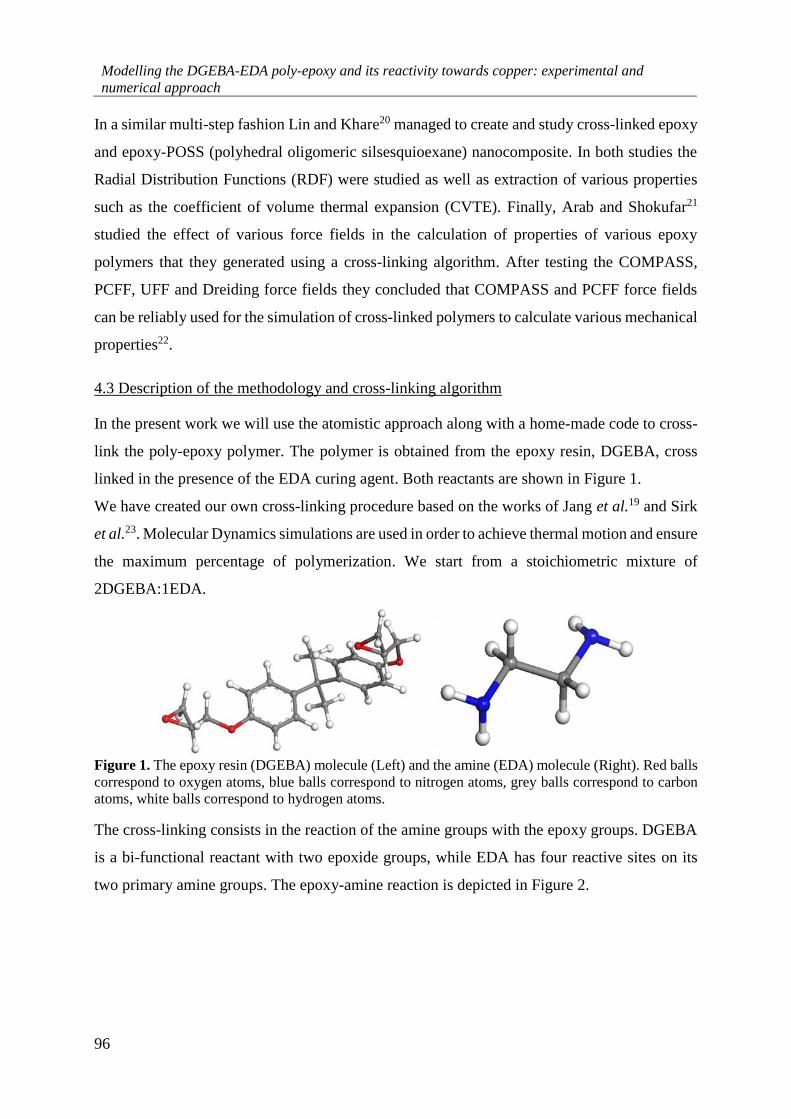
Modelling the DGEBA-EDA poly-epoxy and its reactivity towards copper: experimental and
numerical approach
96
In a similar multi-step fashion Lin and Khare20 managed to create and study cross-linked epoxy
and epoxy-POSS (polyhedral oligomeric silsesquioexane) nanocomposite. In both studies the
Radial Distribution Functions (RDF) were studied as well as extraction of various properties
such as the coefficient of volume thermal expansion (CVTE). Finally, Arab and Shokufar21
studied the effect of various force fields in the calculation of properties of various epoxy
polymers that they generated using a cross-linking algorithm. After testing the COMPASS,
PCFF, UFF and Dreiding force fields they concluded that COMPASS and PCFF force fields
can be reliably used for the simulation of cross-linked polymers to calculate various mechanical
properties22.
4.3 Description of the methodology and cross-linking algorithm
In the present work we will use the atomistic approach along with a home-made code to cross-
link the poly-epoxy polymer. The polymer is obtained from the epoxy resin, DGEBA, cross
linked in the presence of the EDA curing agent. Both reactants are shown in Figure 1.
We have created our own cross-linking procedure based on the works of Jang et al.19 and Sirk
et al.23. Molecular Dynamics simulations are used in order to achieve thermal motion and ensure
the maximum percentage of polymerization. We start from a stoichiometric mixture of
2DGEBA:1EDA.
Figure 1. The epoxy resin (DGEBA) molecule (Left) and the amine (EDA) molecule (Right). Red balls
correspond to oxygen atoms, blue balls correspond to nitrogen atoms, grey balls correspond to carbon
atoms, white balls correspond to hydrogen atoms.
The cross-linking consists in the reaction of the amine groups with the epoxy groups. DGEBA
is a bi-functional reactant with two epoxide groups, while EDA has four reactive sites on its
two primary amine groups. The epoxy-amine reaction is depicted in Figure 2.

Chapter 4: Molecular Dynamics Simulations
97
Figure 2. Epoxy-amine reaction (adapted from Ref24).
The nitrogen atom reacts with one electrophilic carbon of the epoxide ring that opens. The
oxygen atom abstracts a hydrogen atom from the primary amine creating an alcohol group and
a secondary amine. This reaction is repeated to grow epoxy chains and to form the crosslinked
network. We developed a cross-linking code that mimics this reactional scheme. The global
calculations procedure is described step by step on the logigram given in Figure 3.
Figure 3. The multi-step cross-linking logigram.
The logigram is composed of numbered blocks of execution. First, the initial structure of the
liquid mixture is created (1). This is obtained by the use of an external code25 that creates a box
where the two molecules are in stoichiometric analogy (400 DGEBA:200 EDA) in a given
volume. This mixture is equilibrated using MD simulations (2). Then, the cross-linking code

Modelling the DGEBA-EDA poly-epoxy and its reactivity towards copper: experimental and
numerical approach
98
initially searches for reactive pairs in a given search radius (3), and, if unreacted pairs remain,
they are covalently bonded (4&5). Finally, the structure is equilibrated with MD simulations at
each polymerization step. Polymerization/Equilibration cycles continue until the
polymerization rate remain constant.
The logigram can be expressed in a number of Steps:
Step 1: Initial simulation boxes construction and minimization of the systems simulation
The first step is to pack the mixed reactants in a box in order to start the equilibration procedure
with an initial energy minimization and NVE and NVT MD simulations to relax the systems.
To create such boxes, we use the PACKMOL25 code which is an open source code distributed
freely. Detailed instructions on how to produce simulation boxes using the PACKMOL code
are given in Annex E. The code produces a random simulation box, containing the required
number of molecules. Its density is controlled by regulating the spatial coordinates. In our case
we use cubic, simulation boxes and periodic conditions for the simulations. The PACKMOL
code can only produce one configuration for a given density and it is based on the concept of
packing optimization25,26. This is done by minimizing a mathematical function called the merit
function26 which is unique for each set of spatial constraints. Since our simulation boxes are
cubic that means for a given density only one box can be created. For simulating different
simulation boxes for both the monomers, their stoichiometric mixture and for polymerizing
multiple boxes we employ in conjunction with PACKMOL the Materials Studio27 software
suite that has the capability of creating various configurations of cubic simulation boxes that
have the same initial density. Its ability to create this variety of cubic simulation boxes comes
from the application of Monte Carlo simulations28 to create random configurations.
For the calculation of the atomic charges using the RESP procedure29,30, the geometries of the
DGEBA and EDA molecules are calculated at the HF/6-31G* level of theory (see Chapter 3)
with Gaussian0931. RESP29 atomic charges are calculated for individual molecules, for the
dimer model (1 DGEBA-1 EDA) and for the trimer model (2 DGEBA-1 EDA) using the
AmberTools code32. The Generalized Amber Force Field33 (GAFF 1.8) is used to describe the
intra- and inter-molecular interactions. Any missing force field values were calculated using
the AmberTools 16 code32. A cutoff distance of 9 Å (with the buffer of 2 Å) is used for the
Coulomb and van der Waals interactions. The Particle-Particle-Particle Mesh (PPPM)
algorithm34 is used to handle long range interactions.

Chapter 4: Molecular Dynamics Simulations
99
In many cases the initial potential energy calculated with GAFF is high due to the presence of
atom-atom overlaps. Thus the energy must be minimized by equilibrating interatomic forces
and the overlaps must be suppressed. After an energy minimization, the systems are relaxed
and are ready to be used as initial configurations for MD. In general, the conditions that have
to be satisfied for the minimization of the potential energy led to a highly coupled system of
non-linear equations. Solving algorithms are called energy minimization algorithms. In the
current study, the HFTN method was employed because of its higher accuracy35 and its fast
convergence to the minimum.
Step 2: Simulation of pure liquids and mixture
This step involves simulations on pure liquids of DGEBA and EDA, and on their stoichiometric
mixture. One objective of these MD simulations is to validate the force field on pure monomers
for which we know physical and structural properties by experiments and from literature.
Another objective is to obtain a liquid that is at an equilibrium before polymerization.
The molecular dynamics calculations and minimizations are carried out using the LAMMPS36
code. The velocity-Verlet integrator37 is used to integrate the equations of motion. The time
step is 1 fs as we want to observe large motions of atoms. The temperature and pressure are
controlled using the Nosé-Hoover thermostat and barostat methods38,39. The temperature used
in the NVT and NPT ensembles is fixed at 700 K. This high temperature is chosen as an enabler
for moving unreacted monomers in the box vigorously and allowing them to diffuse at larger
distances, reaching other unreacted monomers and thus connecting a larger number of pairs.
The pressure is fixed at 1 atm in NPT in order to avoid any effects of high tensions in the epoxy
network that would result in the failure of the simulation and the “destruction” of the simulation
box as well as structures that are not structurally consistent with reality.
Steps 3, 4 and 5: Cross-linking algorithm
The code for cross-linking is written in the FORTRAN90 ® programming language as it is a
language that has a significant advantage in the execution and resolution of mathematical
problems. FORTRAN’s library support for numerical calculations is unmatched by other
modern programming languages (e.g. C++) and it is still heavily used in scientific fields. For
this reason FORTRAN has some of the best optimizers that exist today in its compilers.

Modelling the DGEBA-EDA poly-epoxy and its reactivity towards copper: experimental and
numerical approach
100
The linking between the N and C atoms and between the O and H atoms is made by updating
the identities of the atoms and bonds, the partial charges and the force field parameters in the
lammps#.data files.
It starts by reading the list of all atoms and finds reactive sites. Then, it searches around a given
cutoff radius (in our case 3Å) for any given site to react with. Two bonds are then created: (i)
between one H of the –NH2 and the epoxy O atom, (ii) between the N and the epoxy –C(H2)
atom. A more detailed procedure on how to fill the input files and execute the code is located
in Annex F.
Step 6: NVE, NVT and NPT simulations
After a polymerization step has been completed, we perform the equilibration of the simulation
box and the preparation for the next polymerization step. Three successive MD calculations are
performed in the NVE, NVT, and NPT ensembles, respectively. NVE simulations relaxes the
solid-liquid system by adjusting bond lengths which recover equilibrium values. But the total
energy of the system remains constant, thus it is not a physical simulation. The NVT simulation
keeps the volume of the box constant while allowing the reacted and unreacted molecules to
move fast. The polymerized regions will not accelerate as much as individual molecules,
allowing them to reach reactive sites to polymerize further in the next cross-linking step. The
NPT simulation simulates physical properties accurately as it is able to describe real
conformations. The scripts for the execution of the MD simulations are all given in detail in
Annex G.
Steps 3 to 6 are repeated until no more pairs can react. This is confirmed by executing NVT
and NPT simulations up to the point where the polymerization percentage is constant in 3
consecutive polymerization steps. The polymerization percentage is calculated by counting the
change of identities over the number of initial reactive pairs.
Step 7: Final annealing
When a polymer structure is formed with a constant polymerization rate (above 90%), the final
structure is annealed to 700K to reach an equilibrium. The structure is then cooled down to
300K where we can calculate properties of the polymer at ambient temperature.
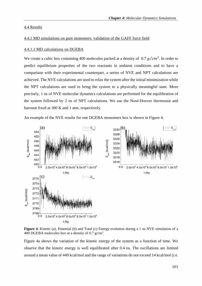
Chapter 4: Molecular Dynamics Simulations
101
4.4 Results
4.4.1 MD simulations on pure monomers: validation of the GAFF force field
4.4.1.1 MD calculations on DGEBA
We create a cubic box containing 400 molecules packed at a density of 0.7 𝑔 𝑐𝑚3⁄ . In order to
predict equilibrium properties of the two reactants in ambient conditions and to have a
comparison with their experimental counterpart, a series of NVE and NPT calculations are
achieved. The NVE calculations are used to relax the system after the initial minimization while
the NPT calculations are used to bring the system to a physically meaningful state. More
precisely, 1 ns of NVE molecular dynamics calculations are performed for the equilibration of
the system followed by 2 ns of NPT calculations. We use the Nosé-Hoover thermostat and
barostat fixed at 300 K and 1 atm, respectively.
An example of the NVE results for one DGEBA monomers box is shown in Figure 4.
Figure 4. Kinetic (a), Potential (b) and Total (c) Energy evolution during a 1 ns NVE simulation of a
400 DGEBA molecules box at a density of 0.7 g/cm3.
Figure 4a shows the variation of the kinetic energy of the system as a function of time. We
observe that the kinetic energy is well equilibrated after 0.4 ns. The oscillations are limited
around a mean value of 449 kcal/mol and the range of variations do not exceed 14 kcal/mol (i.e.

Modelling the DGEBA-EDA poly-epoxy and its reactivity towards copper: experimental and
numerical approach
102
3% of the mean value). Figure 4b shows the variation of the potential energy as function of
time. We also observe a plateau after 0.4 ns as with the kinetic energy. Figure 4c shows the
variation of the total energy of the system which is the addition of the kinetic and potential
energy. A plateau is reached after 0.4 ns that remains until the end of the simulation. We can
conclude that the DGEBA liquid is well equilibrated using the GAFF force field and a
Molecular Dynamics simulation of 1 ns.
We then perform a 2 ns NPT simulation at 300 K and 1 atm, to reach an equilibrium and further
evaluate if the density is close to experimental values. An example of the results of this
simulation is presented in Figure 5.
Figure 5. Temperature (a), pressure (b), overall density (c) and custom (zoom) range density (d)
evolution during a 2ns NPT simulation of a 400 DGEBA molecules box at 300 K and 1 atm.
Figure 5a presents the variation of the temperature as a function of time. We observe that the
temperature is well equilibrated throughout the simulation duration around the value that we
have fixed with the thermostat (300 K). The oscillations are in a limited range of ± 6 K. Figure
5b shows the evolution of the pressure as a function of time. Although the mean value regulated
by the barostat is 1 atm, we observe large fluctuations of up to 1500 atm. This is typical of MD
simulations of condensed phases. Pressure is a macroscopic property of the system and thus
should be considered as an average value over long simulations. Pressure fluctuations are large
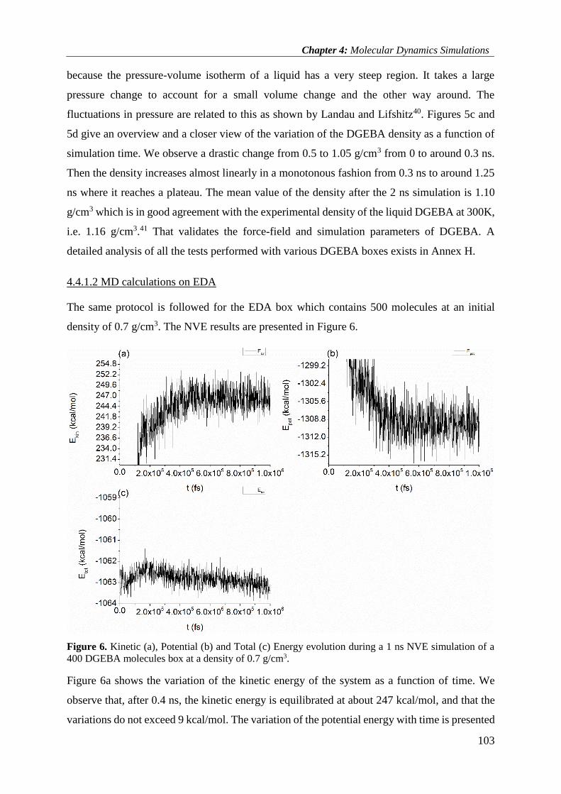
Chapter 4: Molecular Dynamics Simulations
103
because the pressure-volume isotherm of a liquid has a very steep region. It takes a large
pressure change to account for a small volume change and the other way around. The
fluctuations in pressure are related to this as shown by Landau and Lifshitz40. Figures 5c and
5d give an overview and a closer view of the variation of the DGEBA density as a function of
simulation time. We observe a drastic change from 0.5 to 1.05 g/cm3 from 0 to around 0.3 ns.
Then the density increases almost linearly in a monotonous fashion from 0.3 ns to around 1.25
ns where it reaches a plateau. The mean value of the density after the 2 ns simulation is 1.10
g/cm3 which is in good agreement with the experimental density of the liquid DGEBA at 300K,
i.e. 1.16 g/cm3.41 That validates the force-field and simulation parameters of DGEBA. A
detailed analysis of all the tests performed with various DGEBA boxes exists in Annex H.
4.4.1.2 MD calculations on EDA
The same protocol is followed for the EDA box which contains 500 molecules at an initial
density of 0.7 g/cm3. The NVE results are presented in Figure 6.
Figure 6. Kinetic (a), Potential (b) and Total (c) Energy evolution during a 1 ns NVE simulation of a
400 DGEBA molecules box at a density of 0.7 g/cm3.
Figure 6a shows the variation of the kinetic energy of the system as a function of time. We
observe that, after 0.4 ns, the kinetic energy is equilibrated at about 247 kcal/mol, and that the
variations do not exceed 9 kcal/mol. The variation of the potential energy with time is presented

Modelling the DGEBA-EDA poly-epoxy and its reactivity towards copper: experimental and
numerical approach
104
in Figure 6b. We observe a slight decrease up to 0.42 ns where a plateau is reached (-1311
kcal/mol). Figure 6c shows the variation of the total energy of the system which is the addition
of the kinetic and potential energy. We assume that the equilibration is reached after 0.4 ns until
the end of the simulation.
A NPT simulation of a total duration of 2 ns is performed at 300 K and 1 atm to simulate the
ambient conditions that are useful to derive the physical properties of the pure EDA. The results
are presented in Figure 7.
Figure 7. Temperature (a), pressure (b), overall density (c) and custom (zoom) range density (d)
evolution during a 2ns NPT simulation of a 500 EDA molecules box at 300 K and 1 atm.
Figure 7a presents the variation of the temperature as a function of time. We observe that the
temperature is well equilibrated around the value that we have fixed with the thermostat, which
is 300 K. Oscillations are in the range ± 10 K. Figure 7b shows the fluctuation of pressure as a
function on time. Although the value fixed in the barostat is 1 atm, we observe fluctuations up
to 2500 atm. As mentioned above, this is not a major concern since the mean value equals 1
atm. Figure 7c gives an overview of the variation of the density as a function of time and we
can observe a drastic increase from the starting density of 0.70 g/cm3 at t=0 to 0.86 g/cm3 at
t=0.125 ns, where it reaches a plateau. The mean density value after equilibration of the EDA

Chapter 4: Molecular Dynamics Simulations
105
liquid is approximately 0.87 g/cm3 which is in a fairly good accordance with the experimental
value of 0.90 g/cm3 at 300K.42 The series of tests performed on various pure liquid EDA boxes
is shown in detail in Annex I.
In conclusion, the series of tests on both reactants indicate that the parameters chosen and the
force field used are accurate in reproducing experimental data and thus validate our choices.
4.4.2. MD calculations on the 2DGEBA:1EDA liquid mixture
We have shown that the pure monomers are both well equilibrated and that we are able to
reproduce their experimental density. We now move to the next step that is to create an initial
mixture in stoichiometric concentration (2DGEBA:1 EDA). An initial mixture of a total of 600
molecules (400 DGEBA + 200 EDA) is selected. This number of molecules is a good
compromise between saving computational time and having a large-enough number of
molecules relevant to simulate polymer properties accurately.
Figures 8 and 9 show an example of the results of NVE and NPT calculations that are obtained
using 5 ns of NVE calculations and 10 ns of NPT calculations fixed at 300 K and 1 atm. These
much longer calculations are achieved in order to double check that the initial mixture is well
equilibrated before cross-linking.
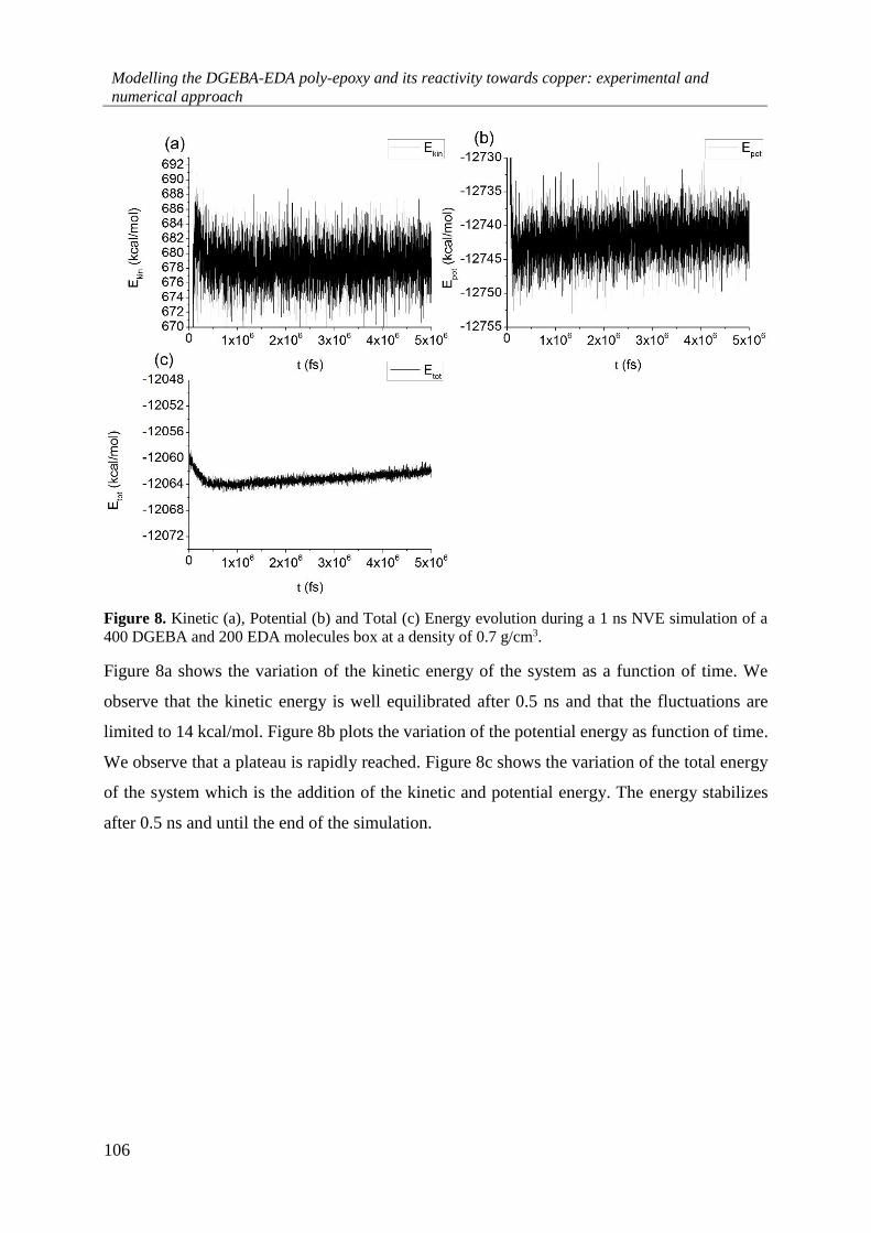
Modelling the DGEBA-EDA poly-epoxy and its reactivity towards copper: experimental and
numerical approach
106
Figure 8. Kinetic (a), Potential (b) and Total (c) Energy evolution during a 1 ns NVE simulation of a
400 DGEBA and 200 EDA molecules box at a density of 0.7 g/cm3.
Figure 8a shows the variation of the kinetic energy of the system as a function of time. We
observe that the kinetic energy is well equilibrated after 0.5 ns and that the fluctuations are
limited to 14 kcal/mol. Figure 8b plots the variation of the potential energy as function of time.
We observe that a plateau is rapidly reached. Figure 8c shows the variation of the total energy
of the system which is the addition of the kinetic and potential energy. The energy stabilizes
after 0.5 ns and until the end of the simulation.

Chapter 4: Molecular Dynamics Simulations
107
Figure 9. Temperature (a), pressure (b), overall density (c) and custom (zoom) range density (d)
evolution during a 10 ns NPT simulation of a 400 DGEBA and 200 EDA molecules box at 300 K and 1
atm.
Figure 9a presents the variation of the temperature as a function of time. We can observe that
the temperature is stable around the value that we fixed in the thermostat. The temperature is
then 300 ± 6 K. Figure 9b shows the fluctuation of pressure as a function on time. The value
regulated by the barostat is 1 atm. We observe fluctuations of up to 2000 atm but the mean
value is correct. Figures 9c and 9d give the overview and focused view of the variation of
density as a function of time. We observe a drastic change from 0.5 to 1.08 g/cm3 from 0 to
around 0.1 ns. Then the density increases almost linearly in a monotonous fashion from 0.1 ns
to around 1.75 ns where it reaches a plateau. The mean density on the plateau is 1.11 g/cm3.
We have also simulated the mixture at 700K and 900K in the NPT ensemble, for two reasons:
(i) to allow a more vigorous movement of molecules, thus increasing the chance of distant
molecules to be crosslinked and (ii) to test higher temperatures needed in the protocol for the
calculation of the Tg. Results are presented in Annex J.
The Radial Distribution Function (RDF) describes how atoms in a simulation box are packed
radially around each other. More generally, the RDF depends on the state of matter. We
calculated the inter- and intra- atomic distances RDF to get first conclusions about the

Modelling the DGEBA-EDA poly-epoxy and its reactivity towards copper: experimental and
numerical approach
108
distributions of the bond lengths and the homogeneity of the box. The RDFs for the two
reactants and their stoichiometric mixture are given in Figure 10.
For the two pure reactants (DGEBA and EDA) and the stoichiometric mixture the RDFs are
calculated after the NPT equilibration before moving to the first polymerization step. We do it
to make sure that the mixture is a homogeneous liquid.
Figure 10. Radial Distribution functions for the inter- and intra- molecular distances for (a) the EDA
molecule, (b) the DGEBA molecule and (c) the stoichiometric mixture.
As shown in Figure 10 we calculated the RDFs with two different conditions: (i) by taking into
account the intramolecular distances (up to two intermediate bonds) and (ii) by taking into
account only the intermolecular distances. The reason behind these two different calculations
is to derive conclusions on the potential overlapping of atoms and to distinguish bond lengths.
In all the simulation boxes, the intermolecular RDFs show that there is a minimum distance of
2Å between any set of atoms, which excludes any possible overlaps. The peaks in the
intramolecular RDFs do not indicate too large bond lengths. The peaks of both DGEBA and
EDA exist in the RDF of the mixture and the N-H (1.01 Å), C-H (1.09 Å), Cph---Cph (1.39 Å),
C-O (1.43 Å) and C-C (1.54 Å) bonds are identified. The peaks identified after the bond length

Chapter 4: Molecular Dynamics Simulations
109
limit (1.54 Å for the C-C bond) are distances between second neighbor atoms. After verifying
the structure of the simulation boxes we move on to the polymerization of the stoichiometric
mixture (2DGEBA:1EDA) boxes.
4.4.3 Polymerization of the 2DGEBA:1EDA system
We create five independent boxes starting from a 600 molecules mixture in stoichiometric
composition. These five boxes will help us test our cross-linking code and its reproducibility in
creating highly cross-linked configurations. All boxes are equilibrated as described above
(NVE and NPT simulations).
In the polymerization code, our initial choice for the cut-off (maximal distance between two
reactive atoms) is 3Å. This relatively short distance ensures that after a polymerization step is
finished, the resulting structure is easy to re-equilibrate using NVE, NVT and NPT calculations
(Step 6).
The conversion rates of the 5 boxes are shown in Figure 11 versus the number of simulation
steps.
Figure 11. Monitoring of the conversion rate during the multi-step cross-linking process, for 5 different
boxes equilibrated at 700K, and 1 box equilibrated at 900K.

Modelling the DGEBA-EDA poly-epoxy and its reactivity towards copper: experimental and
numerical approach
110
We observe that final conversion rates are all above 90% after 11 steps. In the most promising
cases we achieve a conversion rate of 93%. Calculations have been attempted up to 12 steps
without further polymerization. The mobility of the remaining molecules or the steric
availability of the remaining reactive sites is too low at these conversion rates. We also tried to
maximize the conversion rate with an additional box equilibrated in NVT and NPT at 900 K
without more success (conversion rate = 92%). This tends to show that the 93% limit will be
difficult to surpass with our simulation parameters.
In Figure 12 we present the analysis of the distribution of bond lengths after 11 polymerization
steps with the NPT and NVT molecular dynamics fixed at 700K. It helps identifying bonds and
make sure that these lengths are in agreement with chemical bond length. We identify 3 distinct
distributions, centered on 1.10 Å, 1.40 Å, and 1.54 Å. In all this distribution, the bond lengths
that belong in this distributions correspond to O-H (0.96 Å), N-H (1.01 Å), C-H (1.09 Å), Cph-
--Cph (1.39 Å), C-O (1.43 Å) and C-C (1.54 Å) bonds.
Figure 12. Bond lengths distribution after 2 ns of NPT simulation fixed at 700 K and 1 atm of a
polymerized box.

Chapter 4: Molecular Dynamics Simulations
111
The bond length distribution analysis is also performed as a checking protocol at all
polymerization steps (not shown). It never shows bonds over 3 Å throughout the polymerization
procedure, validating the operability of the cross-linking cutoff. The intramolecular and
intermolecular RDFs calculated for Box#1 is shown in Figure 13.
Figure 13. Inter- and intramolecular Radial Distribution Function calculated for the fully polymerized
simulation box
The intramolecular RDF shows a significant peak around 1Å corresponding to the O-H bonds
(length = 0.9Å). We also conclude that there is no significant overlapping as there is no
contribution to the intermolecular RDF before the 2Å point. We proceed with the calculation
of the glass transition temperature.
4.4.4 Glass transition temperature of the model polymer
The glass transition is observed in amorphous materials as it is the case for our poly-epoxy
polymer. It is the physical transition from a hard “glassy” state into a viscous or rubbery state
with the increase of temperature; and it corresponds to the breaking of intermolecular VdW
interactions.
To determine the glass transition temperature with MD simulations, a protocol is followed
based on the paper of Sirk et al.23 First, the procedure consists in heating the polymer at 700 K
for 2 ns and cooling it at a rate of 25 K/ns down to 25 K. Thus we cover a large spectrum of

Modelling the DGEBA-EDA poly-epoxy and its reactivity towards copper: experimental and
numerical approach
112
temperatures. Then we plot the specific volume v (the inverse of the calculated density) as a
function of temperature. The result for Box #4 is shown in Figure 14.
Figure 14. Specific volume as a function of temperature. The intersection of the linear regressions in
the glassy and rubbery temperature regions helps estimating the glass transition temperature.
An elegant procedure to analyze the plot in Figure 14 consists in distinguishing the glassy and
rubbery temperature domains. Actually, although there is a change in physical properties during
the glass transition, it is not considered as a phase transition but rather like a phenomenon that
evolves through an undefined range of temperatures. Temperature regions must then be
identified to fit the linear regimes properly and to estimate the Tg at the intersection. For that
reason we plot the coefficient of thermal volume expansion (CVTE) versus temperature. The
coefficient is calculated via Equation 1:
𝐶𝑉𝑇𝐸 = [(1
𝑣) (
𝜕𝑣
𝜕𝑇)]
𝑃(1)
The term,[(𝜕𝑣
𝜕𝑇)]
𝑃 is calculated from the v-T diagram as presented in Figure 15 using a finite-
difference method in Origin software.

Chapter 4: Molecular Dynamics Simulations
113
Figure 15. Dependence of the coefficient of thermal volume expansion in relation with temperature for
3 different boxes.
The CVTE is constant at a given state and varies in transition states. In Figure 15, the glassy
state region is easily identified up to T = 275 K. At higher temperatures there are no clear
regions. Nevertheless we conditionally place a second limit at T = 450 K. By doing so, we
assume that all points above 575 K are not valid because they exceed known limits for the
CVTE of thermosets in the rubbery region43, i.e. 4x10⁻⁴-8x10⁻⁴ K-1. Consequences are that we
can fit the plot in Figure 14 with a single linear regression calculated from 25 K to 350 K.
Above, there are multiple possibilities for the range of the linear regression. With the regression
proposed in Figure 14, we get a result of a computed Tg of 390±8 K which compares very well
with the experimental glass transition temperature of 391±1 K measured using DSC. The
polymer density is also in very good accordance with bibliography as it was calculated to be
1.115 g/cm3 at 300 K whereas the value obtained through empirical calculations, is 1.142
g/cm3.44 This empirical density is calculated through the relationship 𝜌 = 350 + 120𝑀(𝑘𝑔 ∙
𝑚−3) where M is the molecular weight of the repeat unit. The value of the M parameter is
representative of the poly-epoxy polymer based on the stoichiometry of two molecules of
DGEBA and one of amine.

Modelling the DGEBA-EDA poly-epoxy and its reactivity towards copper: experimental and
numerical approach
114
4.5 Conclusion
In this chapter we fulfill the goal of creating a bulk polymer starting from a stoichiometric liquid
mixture of the two reactants (DGEBA and EDA). To achieve this task we have developed a
home-made cross-linking code that identifies any reactive centers that exist in a distance of less
than 3Å and creates covalent bonds. Through a series of molecular dynamics calculations and
by the use of parameters from the GAFF 1.8 force field we were able to equilibrate and calculate
properties for our pure reactants liquids, the liquid mixtures, as well as for the intermediate
semi-polymerized phases and for the final polymer. The cross-linking is based on a multi-step
approach based on MD equilibration/cross-linking cycles. The characteristics of the final
polymer compare very well with experimental values, in terms of density and Tg. The bulk
poly-epoxy model is in good agreement with the experimental counterpart. The validation of
the model can be continued through the calculation of mechanical properties such as the
Young’s modulus. In addition, a model of the surface was not yet extracted at the end of the
PhD, something that is of great value for future works.
Bibliography
1. Doherty, D. C., Holmes, B. N., Leung, P. & Ross, R. B. Polymerization molecular dynamics
simulations. I. Cross-linked atomistic models for poly(methacrylate) networks. Comput. Theor.
Polym. Sci. 8, 169–178 (1998).
2. Deng, M., Tan, V. B. C. & Tay, T. E. Atomistic modeling: interfacial diffusion and adhesion of
polycarbonate and silanes. Polymer 45, 6399–6407 (2004).
3. Tzoumanekas, C. & Theodorou, D. N. From atomistic simulations to slip-link models of
entangled polymer melts: Hierarchical strategies for the prediction of rheological properties. Curr.
Opin. Solid State Mater. Sci. 10, 61–72 (2006).
4. Auhl, R., Everaers, R., Grest, G. S., Kremer, K. & Plimpton, S. J. Equilibration of long chain
polymer melts in computer simulations. J. Chem. Phys. 119, 12718–12728 (2003).
5. Pakula, T. & Zhulina, E. B. Computer simulation of polymers in thin layers. II. Structure of
polymer melt layers consisting of end‐to‐wall grafted chains. J. Chem. Phys. 95, 4691–4697
(1991).
6. Vogiatzis, G. G., Voyiatzis, E. & Theodorou, D. N. Monte Carlo simulations of a coarse grained
model for an athermal all-polystyrene nanocomposite system. Eur. Polym. J. 47, 699–712 (2011).
7. Theodorou, D. N. & Suter, U. W. Atomistic modeling of mechanical properties of polymeric
glasses. Macromolecules 19, 139–154 (1986).
8. Tsige, M. & Stevens, M. J. Effect of Cross-Linker Functionality on the Adhesion of Highly Cross-
Linked Polymer Networks: A Molecular Dynamics Study of Epoxies. Macromolecules 37, 630–
637 (2004).
9. Bermejo, J. S. & Ugarte, C. M. Chemical Crosslinking of PVA and Prediction of Material
Properties by Means of Fully Atomistic MD Simulations. Macromol. Theory Simul. 18, 259–267
(2009).
10. Bermejo, J. S. & Ugarte, C. M. Influence of Cross-Linking Density on the Glass Transition and
Structure of Chemically Cross-Linked PVA: A Molecular Dynamics Study. Macromol. Theory
Simul. 18, 317–327 (2009).
Chapter 4: Molecular Dynamics Simulations
115
11. Bandyopadhyay, A., Valavala, P. K., Clancy, T. C., Wise, K. E. & Odegard, G. M. Molecular
modeling of crosslinked epoxy polymers: The effect of crosslink density on thermomechanical
properties. Polymer 52, 2445–2452 (2011).
12. Li, C. & Strachan, A. Molecular simulations of crosslinking process of thermosetting polymers.
Polymer 51, 6058–6070 (2010).
13. Nouri, N. & Ziaei-Rad, S. A Molecular Dynamics Investigation on Mechanical Properties of
Cross-Linked Polymer Networks. Macromolecules 44, 5481–5489 (2011).
14. Varshney, V., Patnaik, S. S., Roy, A. K. & Farmer, B. L. A Molecular Dynamics Study of Epoxy-
Based Networks: Cross-Linking Procedure and Prediction of Molecular and Material Properties.
Macromolecules 41, 6837–6842 (2008).
15. Fan, H. B. & Yuen, M. M. F. Material properties of the cross-linked epoxy resin compound
predicted by molecular dynamics simulation. Polymer 48, 2174–2178 (2007).
16. Choi, J., Yu, S., Yang, S. & Cho, M. The glass transition and thermoelastic behavior of epoxy-
based nanocomposites: A molecular dynamics study. Polymer 52, 5197–5203 (2011).
17. Yu, S., Yang, S. & Cho, M. Multiscale modeling of cross-linked epoxy nanocomposites to
characterize the effect of particle size on thermal conductivity. J. Appl. Phys. 110, 124302 (2011).
18. Zeng, Q. H., Yu, A. B. & Lu, G. Q. Multiscale modeling and simulation of polymer
nanocomposites. Prog. Polym. Sci. 33, 191–269 (2008).
19. Jang, C., Sirk, T. W., Andzelm, J. W. & Abrams, C. F. Comparison of Crosslinking Algorithms in
Molecular Dynamics Simulation of Thermosetting Polymers. Macromol. Theory Simul. 24, 260–
270 (2015).
20. Lin, P.-H. & Khare, R. Molecular Simulation of Cross-Linked Epoxy and Epoxy−POSS
Nanocomposite. Macromolecules 42, 4319–4327 (2009).
21. Arab, B. & Shokuhfar, A. Molecular Dynamics Simulation of Cross-Linked Epoxy Polymers: the
Effect of Force Field on the Estimation of Properties. Журнал Нано-Та Електронної Фізики
01013–1 (2013).
22. Masoumi, S., Arab, B. & Valipour, H. A study of thermo-mechanical properties of the cross-
linked epoxy: An atomistic simulation. Polymer 70, 351–360 (2015).
23. Sirk, T. W. et al. High strain rate mechanical properties of a cross-linked epoxy across the glass
transition. Polymer 54, 7048–7057 (2013).
24. Machavaram, V. R. et al. Multi-point monitoring of cross-linking reactions. J. Appl. Polym. Sci.
131, n/a-n/a (2014).
25. Martínez, L., Andrade, R., Birgin, E. G. & Martínez, J. M. PACKMOL: a package for building
initial configurations for molecular dynamics simulations. J. Comput. Chem. 30, 2157–2164
(2009).
26. Martínez, J. M. & Martínez, L. Packing optimization for automated generation of complex
system’s initial configurations for molecular dynamics and docking. J. Comput. Chem. 24, 819–
825 (2003).
27. Materials Studio Materials Modeling & Simulation Application | Dassault Systèmes BIOVIA.
Available at: http://accelrys.com/products/collaborative-science/biovia-materials-studio/.
(Accessed: 3rd October 2017)
28. Akkermans, R. L. C., Spenley, N. A. & Robertson, S. H. Monte Carlo methods in Materials
Studio. Mol. Simul. 39, 1153–1164 (2013).
29. Bayly, C. I., Cieplak, P., Cornell, W. & Kollman, P. A. A well-behaved electrostatic potential
based method using charge restraints for deriving atomic charges: the RESP model. J. Phys.
Chem. 97, 10269–10280 (1993).
30. Cornell, W. D., Cieplak, P., Bayly, C. I. & Kollmann, P. A. Application of RESP charges to
calculate conformational energies, hydrogen bond energies, and free energies of solvation. J. Am.
Chem. Soc. 115, 9620–9631 (1993).
31. Gaussian 09, M. J. Frisch, G. W. Trucks, H. B. Schlegel, G. E. Scuseria, M. A. Robb, J. R.
Cheeseman, G. Scalmani, V. Barone, G. A. Petersson, H. Nakatsuji, X. Li, M. Caricato, A.
Marenich, J. Bloino, B. G. Janesko, R. Gomperts, B. Mennucci, H. P. Hratchian, J. V. Ortiz, A. F.
Izmaylov, J. L. Sonnenberg, D. Williams-Young, F. Ding, F. Lipparini, F. Egidi, J. Goings, B.
Peng, A. Petrone, T. Henderson, D. Ranasinghe, V. G. Zakrzewski, J. Gao, N. Rega, G. Zheng, W.
Liang, M. Hada, M. Ehara, K. Toyota, R. Fukuda, J. Hasegawa, M. Ishida, T. Nakajima, Y.

Modelling the DGEBA-EDA poly-epoxy and its reactivity towards copper: experimental and
numerical approach
116
Honda, O. Kitao, H. Nakai, T. Vreven, K. Throssell, J. A. Montgomery, Jr., J. E. Peralta, F.
Ogliaro, M. Bearpark, J. J. Heyd, E. Brothers, K. N. Kudin, V. N. Staroverov, T. Keith, R.
Kobayashi, J. Normand, K. Raghavachari, A. Rendell, J. C. Burant, S. S. Iyengar, J. Tomasi, M.
Cossi, J. M. Millam, M. Klene, C. Adamo, R. Cammi, J. W. Ochterski, R. L. Martin, K. Morokuma,
O. Farkas, J. B. Foresman, and D. J. Fox, Gaussian, Inc., Wallingford CT, 2016.
32. D.A. Case, D.S. Cerutti, T.E. Cheatham, III, T.A. Darden, R.E. Duke, T.J. Giese, H. Gohlke, A.W.
Goetz, D. Greene, N. Homeyer, S. Izadi, A. Kovalenko, T.S. Lee, S. LeGrand, P. Li, C. Lin, J. Liu,
T. Luchko, R. Luo, D. Mermelstein, K.M. Merz, G. Monard, H. Nguyen, I. Omelyan, A. Onufriev,
F. Pan, R. Qi, D.R. Roe, A. Roitberg, C. Sagui, C.L. Simmerling, W.M. Botello-Smith, J. Swails,
R.C. Walker, J. Wang, R.M. Wolf, X. Wu, L. Xiao, D.M. York and P.A. Kollman (2017), AMBER
2017, University of California, San Francisco.
33. Wang, J., Wolf, R. M., Caldwell, J. W., Kollman, P. A. & Case, D. A. Development and testing of
a general amber force field. J. Comput. Chem. 25, 1157–1174 (2004).
34. Hockney, R. & Eastwood, J. Particle-Particle-Particle-Mesh (P3M) Algorithms. in Computer
simulation using particles 267–304 (Adam Hilger).
35. Chapelle, O. & Erhan, D. Improved preconditioner for hessian free optimization. in In NIPS
Workshop on Deep Learning and Unsupervised Feature Learning (2011).
36. Plimpton, S. Fast Parallel Algorithms for Short-Range Molecular Dynamics. J. Comput. Phys.
117, 1–19 (1995).
37. Verlet, L. Computer ‘Experiments’ on Classical Fluids. I. Thermodynamical Properties of
Lennard-Jones Molecules. Phys. Rev. 159, 98–103 (1967).
38. Hoover, W. G. & Holian, B. L. Kinetic moments method for the canonical ensemble distribution.
Phys. Lett. A 211, 253–257 (1996).
39. Nosé, S. A unified formulation of the constant temperature molecular dynamics methods. J.
Chem. Phys. 81, 511–519 (1984).
40. Landau, L. D. & Lifshitz, E. M. Statistical Physics. (Pergamon Press).
41. DGEBA Epoxy Resin. Available at: http://polymerdatabase.com/polymers/bisphenol-
adiglycidyletherepoxyresin.html. (Accessed: 18th September 2017)
42. Ethylenediamine E26266. NH2CH2CH2NH2 Available at:
http://www.sigmaaldrich.com/catalog/product/sial/e26266. (Accessed: 18th September 2017)
43. Pascault, J. P., Sautereau, H., Verdu, J. & Williams, R. J. J. Glass Transition and Transformation
Diagrams. in Thermosetting Polymers 121 (Marcel Dekker, Inc.).
44. Garcia, F. G., Soares, B. G., Pita, V. J. R. R., Sánchez, R. & Rieumont, J. Mechanical properties
of epoxy networks based on DGEBA and aliphatic amines. J. Appl. Polym. Sci. 106, 2047–2055
(2007).

Conclusions générales et perspectives
117
Conclusions générales et perspectives
Le Chapitre 1 a permis d’introduire les notions générales et les outils théoriques utilisés dans
ce travail. Notre choix a porté sur deux techniques de calculs :
des calculs quantiques statiques (DFT et HF) qui permettent d’obtenir des informations
sur les liaisons chimiques et la structure électronique du polymère avec ou sans
interaction(s) avec le cuivre.
des calculs de dynamique moléculaire qui permettent d'équilibrer les liquides purs de
réactifs et leur mélange et de calculer diverses propriétés structurales et physiques. En
conjonction avec un code de réticulation, ils peuvent aussi conduire à la formation d’un
polymère et au calcul de ses propriétés. Un choix important est réalisé dans ce chapitre :
le champ de force. Nous avons sélectionné GAFF1.8.
Dans le chapitre 2, nous avons développé l'aspect expérimental de ce travail. Le protocole de
synthèse est présenté qui comprend la polymérisation et le post-traitement du polymère dans
des conditions inertes (atmosphère d'argon). Les échantillons de polymères sont déposés sur
des plaquettes de silicium, et laissés à température ambiante pendant 48 h, avant d’être chauffés
à 140 °C pendant 2h pour atteindre un pourcentage de polymérisation élevé. Le pourcentage de
polymérisation est surveillée et la température de transition vitreuse est mesurée et comparée à
la bibliographie1. La rugosité de surface est contrôlée par AFM (autour de 1 nm). Elle est
suffisamment faible pour observer la croissance des films de Cu sans interférence2. La surface
est également caractérisée par XPS et 3 contributions peuvent être placées sous le pic de C1s
pour sa décomposition. Les échantillons de polymère sont ensuite métallisés sous ultravide
(UHV, 1x10⁻⁹ mbar) à la température ambiante à l'aide d'un évaporateur de métaux. On forme
alors des couches minces de Cu d’épaisseur 5-6 nm. Le dépôt provoque la disparition de
l'épaulement C-O (l’une des 3 contributions du pic C1s), nous donnant ainsi une première idée
du mécanisme d'adsorption des atomes de Cu.
Dans le Chapitre 3, nous avons montré que les interprétations des résultats XPS du chapitre
précédent peuvent être largement améliorées en utilisant les données de sortie de calculs
quantiques. Nous avons démontré comment des calculs HF-ΔSCF permettent de simuler le
spectre du C1s grâce aux calculs des décalages chimiques3 (ΔBE) et des intensités relatives des

Modelling the DGEBA-EDA poly-epoxy and its reactivity towards copper: experimental and
numerical approach
118
différentes composantes du pic. Cependant, les calculs de type HF ont été réalisés par le Pr.
P.S. Bagus, à l’université du North Texas4, en collaboration. Afin d’internaliser la démarche,
nous avons décidé de reproduire ces résultats dans le cadre de la théorie DFT (maitrisée en
interne). Le code deMon2k nous a permis d’utiliser la théorie uGTS5–8 et nous avons simulé de
nouveau les spectres XPS avec succès. Les spectres obtenus à partir des deux modes de calculs
(HF et uGTS) révèlent 8 contributions, en lieu et place des 3 contributions déterminées
expérimentalement. Le travail a été poursuivi avec l’adsorption d’un atome de cuivre dans
différentes positions sur le dimère modèle. Au total, 9 sites d'adsorption ont été testés et les
géométries optimisées. Les meilleurs résultats sont obtenus lorsque l'atome de Cu est
chimisorbé en pont sur un atome d’oxygène et un atome de carbone du phényl adjacent. La
simulation du spectre XPS C1s à partir de cette configuration est en bon accord avec
l’expérience. La contribution d’origine C-OH qui se trouvait dans l’épaulement aux hautes
énergies de liaison sur le spectre de la surface nue, est maintenant remplacée par une
contribution C-O-Cu, décalée vers les basses énergies de liaison. L’épaulement est donc très
fortement atténué, en adéquation avec les observations expérimentales avant et après dépôt du
film nanométrique de Cu.
Le chapitre 4 décrit nos efforts pour extraire les propriétés structurales et physiques des liquides
purs de réactifs et de leur mélange, et du polymère final. Le mélange (DGEBA, EDA) est utilisé
pour simuler la réticulation. Un algorithme de réticulation maison9 est appelé en alternance avec
la dynamique moléculaire, de la façon suivante : le mélange est d’abord équilibré à 700 K et 1
atm, ce qui assure une agitation vigoureuse des molécules. Puis chaque étape de réticulation est
réalisée en statique et consiste à lier les atomes réactifs qui se trouvent à 3Å ou moins l’une de
l’autre. A l’issue de ces cycles d’équilibration/réticulation, le pourcentage de polymérisation
maximal se stabilise à 93%. Les structures sont validées par le calcul des distributions de
distances interatomiques, et par la comparaison entre les densités calculée et expérimentale.
Enfin, une méthodologie proposée par Sirk et al.11 est employée pour le calcul de la température
de transition vitreuse, Tg. La Tg calculée (390±8 K) est très proche de la Tg expérimentale
(391±1 K). Par conséquent, même si ce premier modèle volumique pour le poly-epoxy doit
encore être affiné, ces travaux vont permettre l'extraction d'un modèle de surface (slab) pour
procéder à des calculs périodiques DFT et à des adsorptions sur une surface poly-époxy
« bidimensionnelle ».
Conclusions générales et perspectives
119
Nous avons donc réussi à créer, à la fois expérimentalement et numériquement, une surface
poly-époxy adaptée à la métallisation. Nous avons pu étudier le mécanisme d'adsorption de Cu
en utilisant des spectres XPS expérimentaux et calculés. Ce n'était qu’une première étape qui
permettra d'ouvrir la voie pour des travaux futurs:
Le dépôt d'une grande variété de métaux (Al, Ag, Au, Ni, Co, Cr, etc.), dont la réactivité
vis-à-vis du polymère diffère, le calcul des spectres XPS et la comparaison avec leurs
homologues expérimentaux ;
L’obtention des fonctions de distribution (RDF) expérimentalement, par analyse des
diagrammes de diffraction des rayons X (DRX) en travaillant sur le facteur de structure
totale normalisé S(Q) qui correspond à l'intensité mesurée, corrigée du bruit, de la
diffusion Compton, de la diffusion multiple, ainsi que de l'absorption et divers autres
facteurs), pour comparer avec les RDF calculées ;
La décomposition des spectres O1s et N1s à l’aide de nouveaux calculs (DFT, uGTS)
et la comparaison avec la contrepartie expérimentale ;
L’extraction d’un échantillon de surface (slab) du modèle volumique pour des études
DFT périodique et l’adsorption de différents atomes métalliques.
Bibliographie
1. Pascault, J. P., Sautereau, H., Verdu, J. & Williams, R. J. . Thermosetting Polymers. (CRC Press,
2002).
2. Duguet, T. et al. Toward a computational and experimental model of a poly-epoxy surface. Appl.
Surf. Sci. 324, 605–611 (2015).
3. Gavrielides, A., Duguet, T., Esvan, J., Lacaze-Dufaure, C. & Bagus, P. S. A poly-epoxy surface
explored by Hartree-Fock ΔSCF simulations of C1s XPS spectra. J. Chem. Phys. 145, 074703
(2016).
4. Bagus, P. S., Liu, B., McLean, A. D. & Yoshimine, M. CLIPS is a program system to compute ab
initio SCF and correlated wavefunctions for polyatomic systems. It has been developed based on
the publicly available programs in the ALCHEMY package from the IBM San Jose Research
Laboratory.
5. Endo, K., Kaneda, Y., Okada, H., Chong, D. P. & Duffy, P. Analysis of X-ray Photoelectron
Spectra of Eight Polymers by deMon Density-Functional Calculations Using the Model
Oligomers. J. Phys. Chem. 100, 19455–19460 (1996).
6. Otsuka, T., Endo, K., Suhara, M. & Chong, D. P. Theoretical X-ray photoelectron spectra of
polymers by deMon DFT calculations using the model dimers. J. Mol. Struct. 522, 47–60 (2000).
7. Motozaki, W., Otsuka, T., Endo, K. & Chong, D. P. Electron Binding Energies of Si 2p and S 2p
for Si- and S-containing Substances by DFT Calculations Using the Model Molecules. Polym. J.
36, 600–606 (2004).
8. Takaoka, K. et al. Analysis of X-ray photoelectron spectra of electrochemically prepared
polyaniline by DFT calculations using model molecules. J. Mol. Struct. 608, 175–182 (2002).
9. Jang, C., Sirk, T. W., Andzelm, J. W. & Abrams, C. F. Comparison of Crosslinking Algorithms in
Molecular Dynamics Simulation of Thermosetting Polymers. Macromol. Theory Simul. 24, 260–
270 (2015).

Modelling the DGEBA-EDA poly-epoxy and its reactivity towards copper: experimental and
numerical approach
120
10. Garcia, F. G., Soares, B. G., Pita, V. J. R. R., Sánchez, R. & Rieumont, J. Mechanical properties
of epoxy networks based on DGEBA and aliphatic amines. J. Appl. Polym. Sci. 106, 2047–2055
(2007).
11. Sirk, T. W. et al. High strain rate mechanical properties of a cross-linked epoxy across the glass
transition. Polymer 54, 7048–7057 (2013).

Annexes


Annexes
123
Annex A: Generalized Amber Force Field1 (GAFF) parameters and atom types
In order to calculate the energetics of the system that is simulated we must choose a suitable set
of parameters that will serve as inputs to the equations for the calculation of all the interactions
(inter- and intramolecular) we desire to take into account. For our molecules the following
parameters were chosen for input in the .data LAMMPS2 files.
For the EDA molecule we use 4 atom types to describe the molecule (which will be explained
below), 4 bond types, 6 angle types and 2 dihedral types (generic types). The parameters are
inputted in the beginning of the .data file as such:
Masses
1 14.01 # n3
2 12.01 # c3
3 1.008 # hn
4 1.008 # h1
Pair Coeffs # lj/charmm/coul/long
1 0.1700 3.2498 # n3
2 0.1094 3.3996 # c3
3 0.0157 1.0690 # hn
4 0.0157 2.6494 # h1
Bond Coeffs # harmonic
1 325.9 1.4647 # n3-c3
2 392.4 1.0190 # n3-hn
3 300.9 1.5375 # c3-c3
4 330.6 1.0969 # c3-h1
Angle Coeffs # harmonic
1 47.42 109.29 # c3-n3-hn
2 41.40 106.40 # hn-n3-hn
3 66.02 111.04 # n3-c3-c3
4 49.53 109.88 # n3-c3-h1
5 46.39 109.56 # c3-c3-h1
6 39.24 108.46 # h1-c3-h1

Modelling the DGEBA-EDA poly-epoxy and its reactivity towards copper: experimental and
numerical approach
124
Dihedral Coeffs # charmm
1 1.800 3 0 0 # -n3-c3-
2 1.400 3 0 0 # -c3-c3-
For the DGEBA molecule we use 7 atom types to describe the molecule and the parameters for
12 bond types, 23 angle types and 12 generic dihedral types. The parameters are adapted
directly from the force field file where available. For the DGEBA molecule some parameters
are missing from the original file. To counter this problem the missing parameters can be
calculated using the AmberTools3 software tools that can identify and calculate empirically any
parameters missing from a given geometry.
Masses
1 12.01 # ca
2 16.00 # os
3 12.01 # c3
4 12.01 # cx
5 1.008 # ha
6 1.008 # h1
7 1.008 # hc
Pair Coeffs # lj/cut/coul/cut
1 0.0860 3.3996 # ca
2 0.1700 3.0000 # os
3 0.1094 3.3996 # c3
4 0.0860 3.3996 # cx
5 0.0150 2.5996 # ha
6 0.0157 2.4712 # h1
7 0.0157 2.6494 # hc
Bond Coeffs # harmonic
1 461.1 1.3984 # ca-ca
2 376.6 1.3696 # ca-os
3 345.8 1.0860 # ca-ha
4 321.0 1.5156 # ca-c3

Annexes
125
5 308.6 1.4316 # os-c3
6 330.6 1.0969 # c3-h1
7 318.3 1.5184 # c3-cx
8 341.5 1.0890 # cx-h1
9 332.2 1.5041 # cx-cx
10 303.6 1.4368 # cx-os
11 300.9 1.5375 # c3-c3
12 330.6 1.0969 # c3-hc
Angle Coeffs # harmonic
1 69.58 119.20 # ca-ca-os
2 66.62 120.02 # ca-ca-ca
3 48.18 119.88 # ca-ca-ha
4 63.53 120.77 # ca-ca-c3
5 62.52 117.96 # ca-os-c3
6 50.80 109.78 # os-c3-h1
7 68.53 107.87 # os-c3-cx
8 39.24 108.46 # h1-c3-h1
9 46.89 109.68 # cx-c3-h1
10 45.76 115.32 # c3-cx-h1
11 61.62 120.10 # c3-cx-cx
12 66.07 115.68 # c3-cx-os
13 45.49 118.70 # cx-cx-h1
14 49.56 114.93 # os-cx-h1
15 92.94 59.09 # cx-cx-os
16 38.31 115.46 # h1-cx-h1
17 63.15 112.07 # ca-c3-c3
18 63.56 112.24 # ca-c3-ca
19 62.86 111.51 # c3-c3-c3
20 46.34 109.80 # c3-c3-hc
21 39.40 107.58 # hc-c3-hc
22 46.34 109.80 # c3-c3-hc
23 84.30 61.78 # cx-os-cx
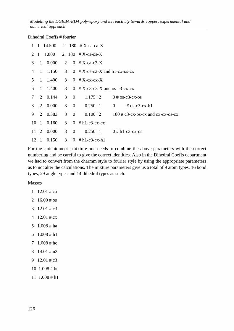
Modelling the DGEBA-EDA poly-epoxy and its reactivity towards copper: experimental and
numerical approach
126
Dihedral Coeffs # fourier
1 1 14.500 2 180 # X-ca-ca-X
2 1 1.800 2 180 # X-ca-os-X
3 1 0.000 2 0 # X-ca-c3-X
4 1 1.150 3 0 # X-os-c3-X and h1-cx-os-cx
5 1 1.400 3 0 # X-cx-cx-X
6 1 1.400 3 0 # X-c3-c3-X and os-c3-cx-cx
7 2 0.144 3 0 1.175 2 0 # os-c3-cx-os
8 2 0.000 3 0 0.250 1 0 # os-c3-cx-h1
9 2 0.383 3 0 0.100 2 180 # c3-cx-os-cx and cx-cx-os-cx
10 1 0.160 3 0 # h1-c3-cx-cx
11 2 0.000 3 0 0.250 1 0 # h1-c3-cx-os
12 1 0.150 3 0 # h1-c3-cx-h1
For the stoichiometric mixture one needs to combine the above parameters with the correct
numbering and be careful to give the correct identities. Also in the Dihedral Coeffs department
we had to convert from the charmm style to fourier style by using the appropriate parameters
as to not alter the calculations. The mixture parameters give us a total of 9 atom types, 16 bond
types, 29 angle types and 14 dihedral types as such:
Masses
1 12.01 # ca
2 16.00 # os
3 12.01 # c3
4 12.01 # cx
5 1.008 # ha
6 1.008 # h1
7 1.008 # hc
8 14.01 # n3
9 12.01 # c3
10 1.008 # hn
11 1.008 # h1

Annexes
127
Pair Coeffs # lj/charmm/coul/long
1 0.0860 3.3996 # ca
2 0.1700 3.0000 # os
3 0.1094 3.3996 # c3
4 0.0860 3.3996 # cx
5 0.0150 2.5996 # ha
6 0.0157 2.4712 # h1
7 0.0157 2.6494 # hc
8 0.1700 3.2498 # n3
9 0.1094 3.3996 # c3
10 0.0157 1.0690 # hn
11 0.0157 2.4712 # h1
Bond Coeffs # harmonic
1 461.1 1.3984 # ca-ca
2 376.6 1.3696 # ca-os
3 345.8 1.0860 # ca-ha
4 321.0 1.5156 # ca-c3
5 308.6 1.4316 # os-c3
6 330.6 1.0969 # c3-h1
7 318.3 1.5184 # c3-cx
8 341.5 1.0890 # cx-h1
9 332.2 1.5041 # cx-cx
10 303.6 1.4368 # cx-os
11 300.9 1.5375 # c3-c3
12 330.6 1.0969 # c3-hc
13 325.9 1.4647 # n3-c3
14 392.4 1.0190 # n3-hn
15 300.9 1.5375 # c3-c3
16 330.6 1.0969 # c3-h1
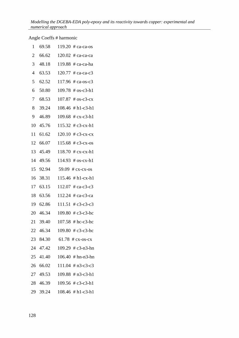
Modelling the DGEBA-EDA poly-epoxy and its reactivity towards copper: experimental and
numerical approach
128
Angle Coeffs # harmonic
1 69.58 119.20 # ca-ca-os
2 66.62 120.02 # ca-ca-ca
3 48.18 119.88 # ca-ca-ha
4 63.53 120.77 # ca-ca-c3
5 62.52 117.96 # ca-os-c3
6 50.80 109.78 # os-c3-h1
7 68.53 107.87 # os-c3-cx
8 39.24 108.46 # h1-c3-h1
9 46.89 109.68 # cx-c3-h1
10 45.76 115.32 # c3-cx-h1
11 61.62 120.10 # c3-cx-cx
12 66.07 115.68 # c3-cx-os
13 45.49 118.70 # cx-cx-h1
14 49.56 114.93 # os-cx-h1
15 92.94 59.09 # cx-cx-os
16 38.31 115.46 # h1-cx-h1
17 63.15 112.07 # ca-c3-c3
18 63.56 112.24 # ca-c3-ca
19 62.86 111.51 # c3-c3-c3
20 46.34 109.80 # c3-c3-hc
21 39.40 107.58 # hc-c3-hc
22 46.34 109.80 # c3-c3-hc
23 84.30 61.78 # cx-os-cx
24 47.42 109.29 # c3-n3-hn
25 41.40 106.40 # hn-n3-hn
26 66.02 111.04 # n3-c3-c3
27 49.53 109.88 # n3-c3-h1
28 46.39 109.56 # c3-c3-h1
29 39.24 108.46 # h1-c3-h1

Annexes
129
Dihedral Coeffs # fourier
1 1 14.500 2 180 # X-ca-ca-X
2 1 1.800 2 180 # X-ca-os-X
3 1 0.000 2 0 # X-ca-c3-X
4 1 1.150 3 0 # X-os-c3-X and h1-cx-os-cx
5 1 1.400 3 0 # X-cx-cx-X
6 1 1.400 3 0 # X-c3-c3-X and os-c3-cx-cx
7 2 0.144 3 0 1.175 2 0 # os-c3-cx-os
8 2 0.000 3 0 0.250 1 0 # os-c3-cx-h1
9 2 0.383 3 0 0.100 2 180 # c3-cx-os-cx and cx-cx-os-cx
10 1 0.160 3 0 # h1-c3-cx-cx
11 2 0.000 3 0 0.250 1 0 # h1-c3-cx-os
12 1 0.150 3 0 # h1-c3-cx-h1
13 1 1.800 3 0 # -n3-c3-
14 1 1.400 3 0 # -c3-c3-
For simulating the crosslinked box in every cross-linking step and the final annealing we must
adjust our coefficients appropriately to include the newly formed bonds which will be
automatically updated by our code. This results in 11 atom types, 17 bond types, 30 angle types
and 14 dihedral types given below:
Masses
1 12.01 # ca
2 16.00 # os
3 12.01 # c3
4 12.01 # cx
5 1.008 # ha
6 1.008 # h1
7 1.008 # hc
8 14.01 # n3
9 12.01 # c3

Modelling the DGEBA-EDA poly-epoxy and its reactivity towards copper: experimental and
numerical approach
130
10 1.008 # hn
11 1.008 # h1
12 16.00 # oh
13 1.008 # ho
Pair Coeffs # lj/charmm/coul/long
1 0.0860 3.3996 # ca
2 0.1700 3.0000 # os
3 0.1094 3.3996 # c3
4 0.0860 3.3996 # cx
5 0.0150 2.5996 # ha
6 0.0157 2.4712 # h1
7 0.0157 2.6494 # hc
8 0.1700 3.2498 # n3
9 0.1094 3.3996 # c3
10 0.0157 1.0690 # hn
11 0.0157 2.4712 # h1
12 0.2104 3.0664 # oh
13 0.0000 0.0000 # ho
Bond Coeffs # harmonic
1 461.1 1.3984 # ca-ca
2 376.6 1.3696 # ca-os
3 345.8 1.0860 # ca-ha
4 321.0 1.5156 # ca-c3
5 308.6 1.4316 # os-c3
6 330.6 1.0969 # c3-h1
7 318.3 1.5184 # c3-cx
8 341.5 1.0890 # cx-h1
9 332.2 1.5041 # cx-cx
10 303.6 1.4368 # cx-os

Annexes
131
11 300.9 1.5375 # c3-c3
12 330.6 1.0969 # c3-hc
13 325.9 1.4647 # n3-c3
14 392.4 1.0190 # n3-hn
15 300.9 1.5375 # c3-c3
16 330.6 1.0969 # c3-h1
17 371.4 0.9730 # ho-oh
Angle Coeffs # harmonic
1 69.58 119.20 # ca-ca-os
2 66.62 120.02 # ca-ca-ca
3 48.18 119.88 # ca-ca-ha
4 63.53 120.77 # ca-ca-c3
5 62.52 117.96 # ca-os-c3
6 50.80 109.78 # os-c3-h1
7 68.53 107.87 # os-c3-cx
8 39.24 108.46 # h1-c3-h1
9 46.89 109.68 # cx-c3-h1
10 45.76 115.32 # c3-cx-h1
11 61.62 120.10 # c3-cx-cx
12 66.07 115.68 # c3-cx-os
13 45.49 118.70 # cx-cx-h1
14 49.56 114.93 # os-cx-h1
15 92.94 59.09 # cx-cx-os
16 38.31 115.46 # h1-cx-h1
17 63.15 112.07 # ca-c3-c3
18 63.56 112.24 # ca-c3-ca
19 62.86 111.51 # c3-c3-c3
20 46.34 109.80 # c3-c3-hc
21 39.40 107.58 # hc-c3-hc

Modelling the DGEBA-EDA poly-epoxy and its reactivity towards copper: experimental and
numerical approach
132
22 46.34 109.80 # c3-c3-hc
23 84.30 61.78 # cx-os-cx
24 47.42 109.29 # c3-n3-hn
25 41.40 106.40 # hn-n3-hn
26 66.02 111.04 # n3-c3-c3
27 49.53 109.88 # n3-c3-h1
28 46.39 109.56 # c3-c3-h1
29 39.24 108.46 # h1-c3-h1
30 47.38 107.26 # c3-oh-ho
Dihedral Coeffs # fourier
1 1 14.500 2 180 # X-ca-ca-X
2 1 1.800 2 180 # X-ca-os-X
3 1 0.000 2 0 # X-ca-c3-X
4 1 1.150 3 0 # X-os-c3-X and h1-cx-os-cx
5 1 1.400 3 0 # X-cx-cx-X
6 1 1.400 3 0 # X-c3-c3-X and os-c3-cx-cx
7 2 0.144 3 0 1.175 2 0 # os-c3-cx-os
8 2 0.000 3 0 0.250 1 0 # os-c3-cx-h1
9 2 0.383 3 0 0.100 2 180 # c3-cx-os-cx and cx-cx-os-cx
10 1 0.160 3 0 # h1-c3-cx-cx
11 2 0.000 3 0 0.250 1 0 # h1-c3-cx-os
12 1 0.150 3 0 # h1-c3-cx-h1
13 1 1.800 3 0 # -n3-c3-
14 1 1.400 3 0 # -c3-c3-

Annexes
133
The atom types given throughout this Annex represent the following atoms:
ca represents an sp2 aromatic carbon
os represents an sp3 oxygen in ethers and esters
c3 represents an sp3 carbon
cx represents an sp3 carbon in three-membered rings
ha represents a hydrogen on aromatic carbon
h1 represents a hydrogen on aliphatic carbon with 1 electron-withdrawal group
hc represents a hydrogen on aliphatic carbon
n3 represents an sp3 nitrogen with 3 substitutes
hn represents hydrogen on nitrogen
oh represents sp3 oxygen in hydroxyl groups
ho represents hydrogen on oxygen
Bibliography
1. Wang, J., Wolf, R. M., Caldwell, J. W., Kollman, P. A. & Case, D. A. Development and testing of
a general amber force field. J. Comput. Chem. 25, 1157–1174 (2004).
2. Plimpton, S. Fast Parallel Algorithms for Short-Range Molecular Dynamics. J. Comput. Phys. 117,
1–19 (1995).
3. D.A. Case, D.S. Cerutti, T.E. Cheatham, III, T.A. Darden, R.E. Duke, T.J. Giese, H. Gohlke, A.W.
Goetz, D. Greene, N. Homeyer, S. Izadi, A. Kovalenko, T.S. Lee, S. LeGrand, P. Li, C. Lin, J. Liu,
T. Luchko, R. Luo, D. Mermelstein, K.M. Merz, G. Monard, H. Nguyen, I. Omelyan, A. Onufriev, F.
Pan, R. Qi, D.R. Roe, A. Roitberg, C. Sagui, C.L. Simmerling, W.M. Botello-Smith, J. Swails, R.C.
Walker, J. Wang, R.M. Wolf, X. Wu, L. Xiao, D.M. York and P.A. Kollman (2017), AMBER 2017,
University of California, San Francisco.

Modelling the DGEBA-EDA poly-epoxy and its reactivity towards copper: experimental and
numerical approach
134
Annex B: The velocity Verlet algorithm
Verlet integration1 is a numerical method that is used for the integration of Newtonian equations
of motion. It is commonly used in Molecular Dynamics simulations to calculate the trajectories
of the molecules in simulation boxes as they evolve in time. It presents greater stability in
comparison with the much simpler Euler method and due to its time-reversibility (the ability to
follow the trajectory backwards to the point that it begun) and area preserving (the ability to
solve the equations of Newton and represent them on an phase-area preserving map thus being
in accordance with Liouville’s2 theorem) properties makes it indispensable for use in our
simulations.
In the velocity Verlet algorithm the velocity and position are calculated at the current time step
as time evolves. This is not the case for other algorithms such as the Leapfrog algorithm giving
an advantage of performing timesteps of various sizes and maintaining stability. The velocity
Verlet, as the name suggests utilizes velocity to calculate the first timestep equations presented
in the Basic Verlet algorithm:
𝑟(𝑡 + 𝛥𝑡) = 𝑟(𝑡) + ��(𝑡)𝛥𝑡 +1
2��(𝑡)𝛥𝑡2 (1)
��(𝑡 + 𝛥𝑡) = ��(𝑡) +��(𝑡) + ��(𝑡 + 𝛥𝑡)
2𝛥𝑡 (2)
The velocity Verlet algorithm does not need to keep track of the velocity at every timestep
making it less memory consuming.
The implementation of the algorithm is summed in the following steps:
1. Calculate �� (𝑡 +1
2𝛥𝑡) = ��(𝑡) +
1
2��(𝑡)𝛥𝑡
2. Calculate 𝑟(𝑡 + 𝛥𝑡) = 𝑟(𝑡) + �� (𝑡 +1
2𝛥𝑡) 𝛥𝑡
3. Derive ��(𝑡 + 𝛥𝑡) using 𝑟(𝑡 + 𝛥𝑡)
4. Calculate ��(𝑡 + 𝛥𝑡) = �� (𝑡 +1
2𝛥𝑡) +
1
2��(𝑡 + 𝛥𝑡)𝛥𝑡
What needs to be noted is that the acceleration ��(𝑡 + 𝛥𝑡) depends ony on the position 𝑟(𝑡 + 𝛥𝑡)
and not on the velocity.
Bibliography
1. Verlet, L. Computer ‘Experiments’ on Classical Fluids. I. Thermodynamical Properties of Lennard-
Jones Molecules. Phys. Rev. 159, 98–103 (1967).
2. Nelson, E. A proof of Liouville’s theorem. Proc. Am. Math. Soc. 12, 995 (1961).

Annexes
135
Annex C: Structure comparison of the dimer molecule optimized using different
computational conditions
This Annex will provide the optimization results for the optimization of the dimer molecule
under different computational conditions (e.g. various exchange-correlation potentials and basis
sets) to compare the various structures produced. All of the calculations were executed using
the deMon2k code1. Table 1 contains the 3 sets of computational parameters that were used for
the optimization of the geometry of the dimer molecules and the total energy of the molecule
after each optimization.
Table 1. Optimization results for the dimer molecule under various computational conditions.
Structure
#
Basis
Set
Exchange-
Correlation
potential
SCF
tolerance
(μHartree)
Optimization
Tolerance
(Å)
Etot
(Hartree)
1 DZVP B88-LYP 1x10⁻⁷ 1x10⁻⁴ -1305.94
2 TZVP B88-LYP 1x10⁻⁷ 1x10⁻⁴ -1306.01
3 TZVP B88-PW91 1x10⁻⁹ 1x10⁻⁴ -1306.35
The dimer geometries optimized with the conditions given in Table 1 are shown in Figure 1.
Figure 1. The 3 dimer molecule structures after optimization under different computational parameters
(green is used to symbolize C atoms, blue for N atoms, red for O atoms and white for H atoms).

Modelling the DGEBA-EDA poly-epoxy and its reactivity towards copper: experimental and
numerical approach
136
By merely looking at the 3 dimer molecule structures we can see the effect of the change of the
computational parameters in the geometry optimization of the dimer molecule. A very good
indicator apart from the positions of the hydrogens connected to the nitrogen atoms is the final
position of the –CH3 carbons. We further analyze the dimer structures in Table 2 by comparing
various bond lengths existing in the dimer molecule.
Table 2. Bond length comparison for the structural analysis of the 3 dimer molecules
Dimer
Structure #
Cep-Oep
(Å)
Cph-Cph
(Å)
C-N
(Å)
N-H
(Å)
C-H
(Å)
C-O
(Å)
C-C
(Å)
1 1.46 1.40 1.47 1.03 1.11 1.45 1.53
2 1.46 1.40 1.48 1.02 1.10 1.45 1.54
3 1.45 1.40 1.48 1.02 1.10 1.44 1.53
Experimental 1.44 1.39 1.47 1.01 1.09 1.43 1.54
We can see that although different geometries and by expansion different atom orientations are
produced by changing the computational parameters there is no significant change in the bond
lengths. We chose the computational parameters used to optimize the third structure for the
XPS initial state calculations by taking into account studies2,3 on the functional dependence of
calculated core energies. It is also worth noting that all the calculated bond lengths are in good
accordance with experimental bond lengths in similar molecules4,5.
Bibliography
1. Kostar, A. M. et al. A.M. Koster, G. Geudtner, P. Calaminici, M.E. Casida, V.D. Dominguez, R.
Flores-Moreno, G.U. Gamboa, A. Goursot, T. Heine, A. Ipatov, F. Janetzko, J.M. del Campo, J. U.
Reveles, A. Vela, B. Zuniga-Gutierrez, and D.R. Salahub, deMon2k, Version 3.0.6, The deMon
developers, Cinvestav, Mexico City (2011). (2014).
2. Takahashi, O. & Pettersson, L. G. M. Functional dependence of core-excitation energies. J. Chem.
Phys. 121, 10339–10345 (2004).
3. Jacobsen, H. & Cavallo, L. Directions for Use of Density Functional Theory: A Short Instruction
Manual for Chemists. in Handbook of Computational Chemistry (ed. Leszczynski, J.) 95–133
(Springer Netherlands, 2012). doi:10.1007/978-94-007-0711-5_4
4. Ellis, B. Chemistry and Technology of Epoxy Resins. (Springer-Science+Business Media, 1993).
5. Computational Chemistry Comparison and Benchmark DataBase (CCCBDB). Available at:
http://cccbdb.nist.gov/.

Annexes
137
Annex D: Comparison between RESP and AM1-BCC methodologies for partial
charge calculations of the EDA, DGEBA, dimer and trimer molecules
We compare the two methodologies for the calculations of the charges using the RESP and
AM1-BCC protocol as described in chapter 3. Results for the calculated of the EDA molecule
using both methodologies are shown in Table 1.
Table 1. EDA net charges (in e) calculated using the RESP and AM1-BCC methodologies.
Atom ID RESP AM1-BCC
N1 -0.9375 -0.9168
C2 0.2930 0.1568
H3 0.3301 0.3493
H4 0.3301 0.3493
C5 0.2811 0.1568
N6 -0.9341 -0.9168
H7 0.3306 0.3493
H8 0.3306 0.3493
H9 -0.0071 0.0307
H10 -0.0070 0.0307
H11 -0.0049 0.0307
H12 -0.0049 0.0307
0 1.04x10⁻¹⁶
The results for the DGEBA molecule are shown in Table 2.
Table 2. DGEBA net charges (in e) calculated using the RESP and AM1-BCC methodologies
Atom ID RESP AM1-BCC
C1 -0.3833 -0.0861
O1 -0.4339 -0.3244
C2 0.1085 0.1329
C3 0.4647 0.0486
C4 -0.3528 -0.0861
C5 -0.0932 -0.1013
C6 -0.3173 -0.1748
C7 0.4577 0.1116
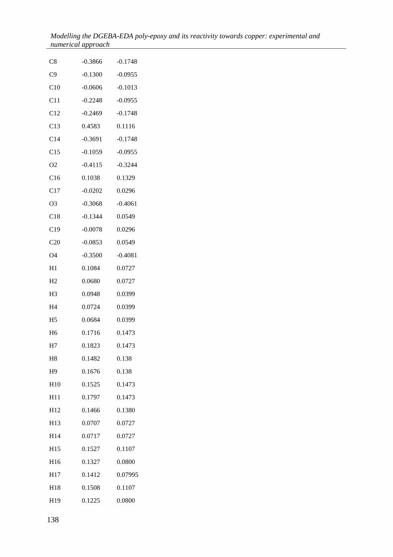
Modelling the DGEBA-EDA poly-epoxy and its reactivity towards copper: experimental and
numerical approach
138
C8 -0.3866 -0.1748
C9 -0.1300 -0.0955
C10 -0.0606 -0.1013
C11 -0.2248 -0.0955
C12 -0.2469 -0.1748
C13 0.4583 0.1116
C14 -0.3691 -0.1748
C15 -0.1059 -0.0955
O2 -0.4115 -0.3244
C16 0.1038 0.1329
C17 -0.0202 0.0296
O3 -0.3068 -0.4061
C18 -0.1344 0.0549
C19 -0.0078 0.0296
C20 -0.0853 0.0549
O4 -0.3500 -0.4081
H1 0.1084 0.0727
H2 0.0680 0.0727
H3 0.0948 0.0399
H4 0.0724 0.0399
H5 0.0684 0.0399
H6 0.1716 0.1473
H7 0.1823 0.1473
H8 0.1482 0.138
H9 0.1676 0.138
H10 0.1525 0.1473
H11 0.1797 0.1473
H12 0.1466 0.1380
H13 0.0707 0.0727
H14 0.0717 0.0727
H15 0.1527 0.1107
H16 0.1327 0.0800
H17 0.1412 0.07995
H18 0.1508 0.1107
H19 0.1225 0.0800
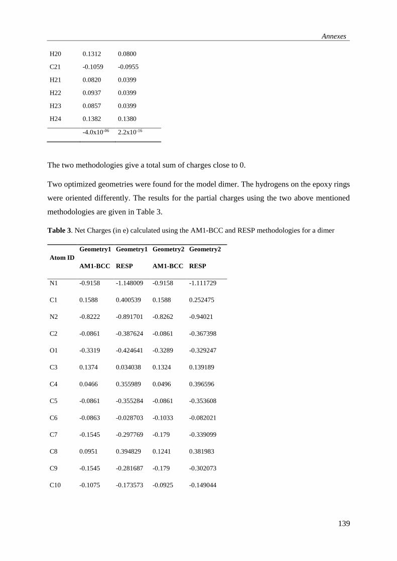
Annexes
139
H20 0.1312 0.0800
C21 -0.1059 -0.0955
H21 0.0820 0.0399
H22 0.0937 0.0399
H23 0.0857 0.0399
H24 0.1382 0.1380
-4.0x10-06 2.2x10⁻¹⁶
The two methodologies give a total sum of charges close to 0.
Two optimized geometries were found for the model dimer. The hydrogens on the epoxy rings
were oriented differently. The results for the partial charges using the two above mentioned
methodologies are given in Table 3.
Table 3. Net Charges (in e) calculated using the AM1-BCC and RESP methodologies for a dimer
Atom ID
Geometry1
AM1-BCC
Geometry1
RESP
Geometry2
AM1-BCC
Geometry2
RESP
N1 -0.9158 -1.148009 -0.9158 -1.111729
C1 0.1588 0.400539 0.1588 0.252475
N2 -0.8222 -0.891701 -0.8262 -0.94021
C2 -0.0861 -0.387624 -0.0861 -0.367398
O1 -0.3319 -0.424641 -0.3289 -0.329247
C3 0.1374 0.034038 0.1324 0.139189
C4 0.0466 0.355989 0.0496 0.396596
C5 -0.0861 -0.355284 -0.0861 -0.353608
C6 -0.0863 -0.028703 -0.1033 -0.082021
C7 -0.1545 -0.297769 -0.179 -0.339099
C8 0.0951 0.394829 0.1241 0.381983
C9 -0.1545 -0.281687 -0.179 -0.302073
C10 -0.1075 -0.173573 -0.0925 -0.149044

Modelling the DGEBA-EDA poly-epoxy and its reactivity towards copper: experimental and
numerical approach
140
C11 -0.1063 -0.071127 -0.1053 -0.087543
C12 -0.0915 -0.068835 -0.0925 -0.091543
C13 -0.179 -0.426182 -0.18 -0.374004
C14 0.1251 0.494092 0.1251 0.500323
C15 -0.179 -0.304987 -0.18 -0.364288
C16 -0.0915 -0.154394 -0.0925 -0.12795
O2 -0.3439 -0.38778 -0.3349 -0.472696
C17 0.0894 -0.041275 0.1244 0.067174
C18 0.1361 0.373958 0.1381 0.285328
O3 -0.6048 -0.65015 -0.6048 -0.706632
C19 0.1708 0.190518 0.1338 0.333346
C20 0.0321 0.032959 0.0611 -0.061955
C21 0.0554 -0.07183 0.0544 -0.09444
O4 -0.4036 -0.35832 -0.4036 -0.307381
H1 0.0687 0.123789 0.0562 0.086759
H2 0.0687 0.077204 0.0562 0.03605
H3 0.0402 0.099442 0.039533 0.097501
H4 0.0402 0.086998 0.039533 0.072188
H5 0.0402 0.076035 0.039533 0.079092
H6 0.143 0.169957 0.143 0.172479
H7 0.143 0.172577 0.143 0.136348
H8 0.139 0.154796 0.138 0.15688
H9 0.1385 0.1473 0.1375 0.137441
H10 0.1425 0.189308 0.1435 0.192658
H11 0.1425 0.154282 0.1435 0.163294
H12 0.1385 0.16543 0.1375 0.155477
H13 0.0532 0.056936 0.0552 0.071582
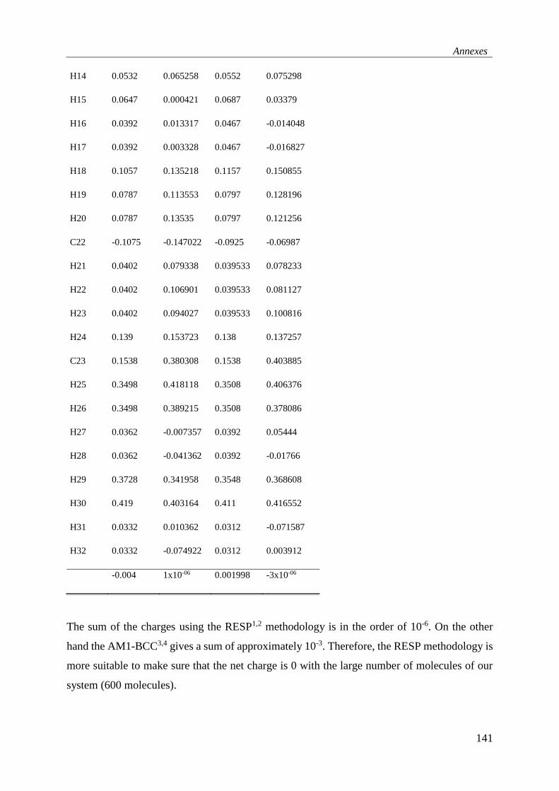
Annexes
141
H14 0.0532 0.065258 0.0552 0.075298
H15 0.0647 0.000421 0.0687 0.03379
H16 0.0392 0.013317 0.0467 -0.014048
H17 0.0392 0.003328 0.0467 -0.016827
H18 0.1057 0.135218 0.1157 0.150855
H19 0.0787 0.113553 0.0797 0.128196
H20 0.0787 0.13535 0.0797 0.121256
C22 -0.1075 -0.147022 -0.0925 -0.06987
H21 0.0402 0.079338 0.039533 0.078233
H22 0.0402 0.106901 0.039533 0.081127
H23 0.0402 0.094027 0.039533 0.100816
H24 0.139 0.153723 0.138 0.137257
C23 0.1538 0.380308 0.1538 0.403885
H25 0.3498 0.418118 0.3508 0.406376
H26 0.3498 0.389215 0.3508 0.378086
H27 0.0362 -0.007357 0.0392 0.05444
H28 0.0362 -0.041362 0.0392 -0.01766
H29 0.3728 0.341958 0.3548 0.368608
H30 0.419 0.403164 0.411 0.416552
H31 0.0332 0.010362 0.0312 -0.071587
H32 0.0332 -0.074922 0.0312 0.003912
-0.004 1x10-06 0.001998 -3x10-06
The sum of the charges using the RESP1,2 methodology is in the order of 10-6. On the other
hand the AM1-BCC3,4 gives a sum of approximately 10-3. Therefore, the RESP methodology is
more suitable to make sure that the net charge is 0 with the large number of molecules of our
system (600 molecules).
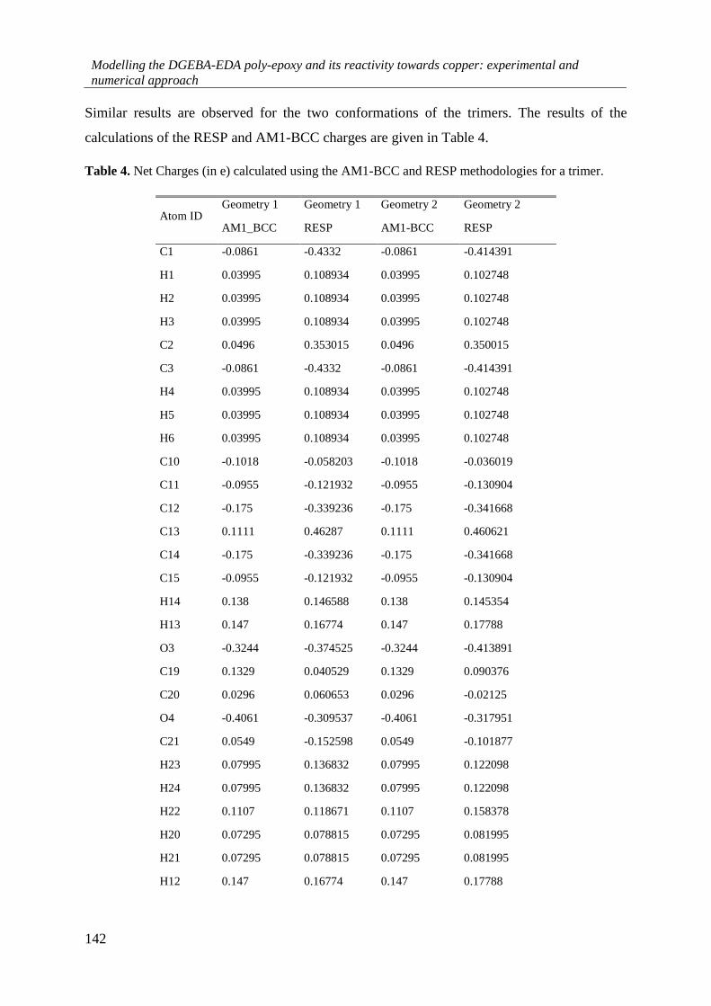
Modelling the DGEBA-EDA poly-epoxy and its reactivity towards copper: experimental and
numerical approach
142
Similar results are observed for the two conformations of the trimers. The results of the
calculations of the RESP and AM1-BCC charges are given in Table 4.
Table 4. Net Charges (in e) calculated using the AM1-BCC and RESP methodologies for a trimer.
Atom ID Geometry 1
AM1_BCC
Geometry 1
RESP
Geometry 2
AM1-BCC
Geometry 2
RESP
C1 -0.0861 -0.4332 -0.0861 -0.414391
H1 0.03995 0.108934 0.03995 0.102748
H2 0.03995 0.108934 0.03995 0.102748
H3 0.03995 0.108934 0.03995 0.102748
C2 0.0496 0.353015 0.0496 0.350015
C3 -0.0861 -0.4332 -0.0861 -0.414391
H4 0.03995 0.108934 0.03995 0.102748
H5 0.03995 0.108934 0.03995 0.102748
H6 0.03995 0.108934 0.03995 0.102748
C10 -0.1018 -0.058203 -0.1018 -0.036019
C11 -0.0955 -0.121932 -0.0955 -0.130904
C12 -0.175 -0.339236 -0.175 -0.341668
C13 0.1111 0.46287 0.1111 0.460621
C14 -0.175 -0.339236 -0.175 -0.341668
C15 -0.0955 -0.121932 -0.0955 -0.130904
H14 0.138 0.146588 0.138 0.145354
H13 0.147 0.16774 0.147 0.17788
O3 -0.3244 -0.374525 -0.3244 -0.413891
C19 0.1329 0.040529 0.1329 0.090376
C20 0.0296 0.060653 0.0296 -0.02125
O4 -0.4061 -0.309537 -0.4061 -0.317951
C21 0.0549 -0.152598 0.0549 -0.101877
H23 0.07995 0.136832 0.07995 0.122098
H24 0.07995 0.136832 0.07995 0.122098
H22 0.1107 0.118671 0.1107 0.158378
H20 0.07295 0.078815 0.07295 0.081995
H21 0.07295 0.078815 0.07295 0.081995
H12 0.147 0.16774 0.147 0.17788

Annexes
143
H11 0.138 0.146588 0.138 0.145354
C4 -0.1048 -0.052125 -0.1048 -0.044194
C9 -0.09225 -0.108933 -0.09225 -0.10885
C8 -0.17975 -0.36552 -0.17975 -0.375811
H9 0.14325 0.174113 0.14325 0.181992
H10 0.138 0.144508 0.138 0.143788
C5 -0.09225 -0.108933 -0.09225 -0.10885
H7 0.138 0.144508 0.138 0.143788
C6 -0.17975 -0.36552 -0.17975 -0.375811
H8 0.14325 0.174113 0.14325 0.181992
C7 0.1241 0.479457 0.1241 0.490312
O1 -0.3369 -0.397127 -0.3369 -0.439557
C16 0.1254 0.044581 0.1254 0.090049
H15 0.05545 0.060631 0.05545 0.058156
H16 0.05545 0.060631 0.05545 0.058156
C17 0.1381 0.330209 0.1381 0.361923
O2 -0.6113 -0.659974 -0.6113 -0.708317
H56 0.4225 0.3997 0.4225 0.425393
H17 0.0582 0.011692 0.0582 0.005945
C18 0.1418 0.008734 0.1418 -0.125794
H18 0.0562 0.058102 0.0562 0.114422
H19 0.0562 0.058102 0.0562 0.114422
N2 -0.7746 -0.415815 -0.7746 -0.521536
C22 0.1768 -0.19457 0.1768 0.060019
C44 0.1528 0.495311 0.1528 0.432458
N1 -0.9178 -1.105928 -0.9178 -1.117585
H49 0.3503 0.401102 0.3503 0.400068
H50 0.3503 0.401102 0.3503 0.400068
H54 0.0332 -0.057232 0.0332 -0.030174
H55 0.0332 -0.057232 0.0332 -0.030174
H51 0.0422 0.109992 0.0422 0.054656
H52 0.0422 0.109992 0.0422 0.054656
C40 0.1418 0.008734 0.1418 -0.125794
C39 0.1381 0.330209 0.1381 0.361923
C38 0.1254 0.044581 0.1254 0.090049

Modelling the DGEBA-EDA poly-epoxy and its reactivity towards copper: experimental and
numerical approach
144
O6 -0.3369 -0.397127 -0.3369 -0.439557
C35 0.1241 0.479457 0.1241 0.490312
C34 -0.17975 -0.36552 -0.17975 -0.375811
C33 -0.09225 -0.108933 -0.09225 -0.10885
C32 -0.1048 -0.052125 -0.1048 -0.044194
C25 0.0496 0.353015 0.0496 0.350015
C23 -0.0861 -0.4332 -0.0861 -0.414391
H45 0.03995 0.108934 0.03995 0.102748
H46 0.03995 0.108934 0.03995 0.102748
H47 0.03995 0.108934 0.03995 0.102748
C26 -0.0861 -0.4332 -0.0861 -0.414391
H27 0.03995 0.108934 0.03995 0.102748
H28 0.03995 0.108934 0.03995 0.102748
H29 0.03995 0.108934 0.03995 0.102748
C27 -0.1018 -0.058203 -0.1018 -0.036019
C31 -0.0955 -0.121932 -0.0955 -0.130904
C30 -0.175 -0.339236 -0.175 -0.341668
C29 0.1111 0.46287 0.1111 0.460621
O5 -0.3244 -0.374525 -0.3244 -0.413891
C24 0.1329 0.040529 0.1329 0.090376
C41 0.0296 0.060653 0.0296 -0.02125
C42 0.0549 -0.152598 0.0549 -0.101877
O8 -0.4061 -0.309537 -0.4061 -0.317951
H43 0.07995 0.136832 0.07995 0.122098
H44 0.07995 0.136832 0.07995 0.122098
H42 0.1107 0.118671 0.1107 0.158378
H25 0.07295 0.078815 0.07295 0.081995
H26 0.07295 0.078815 0.07295 0.081995
C28 -0.175 -0.339236 -0.175 -0.341668
H30 0.147 0.16774 0.147 0.17788
C43 -0.0955 -0.121932 -0.0955 -0.130904
H48 0.138 0.146588 0.138 0.145354
H31 0.147 0.16774 0.147 0.17788
H32 0.138 0.146588 0.138 0.145354
C37 -0.09225 -0.108933 -0.09225 -0.10885

Annexes
145
C36 -0.17975 -0.36552 -0.17975 -0.375811
H35 0.14325 0.174113 0.14325 0.181992
H36 0.138 0.144508 0.138 0.143788
H33 0.138 0.144508 0.138 0.143788
H34 0.14325 0.174113 0.14325 0.181992
H37 0.05545 0.060631 0.05545 0.058156
H38 0.05545 0.060631 0.05545 0.058156
O7 -0.6113 -0.659974 -0.6113 -0.708317
H53 0.4225 0.3997 0.4225 0.425393
H39 0.0582 0.011692 0.0582 0.005945
H40 0.0562 0.058102 0.0562 0.114422
H41 0.0562 0.058102 0.0562 0.114422
Total 0.004 6x10-06 0.004 4.16334x10⁻¹⁶
There is no need to go beyond the trimer molecule. The aim of using both a dimer and a trimer
in our calculations was to calculate the partial charges that will be used in the cross-linking
procedure in various intermediate states of connectivity of the active centers that take place in
the polymerization procedure. The trimer is used to saturate the amine site with two DGEBA
molecules. Considering the number of molecules, the RESP methodology is the best choice.
Bibliography
1. Bayly, C. I., Cieplak, P., Cornell, W. & Kollman, P. A. A well-behaved electrostatic potential based
method using charge restraints for deriving atomic charges: the RESP model. J. Phys. Chem. 97,
10269–10280 (1993).
2. Cornell, W. D., Cieplak, P., Bayly, C. I. & Kollmann, P. A. Application of RESP charges to
calculate conformational energies, hydrogen bond energies, and free energies of solvation. J. Am.
Chem. Soc. 115, 9620–9631 (1993).
3. Jakalian, A., Bush, B. L., Jack, D. B. & Bayly, C. I. Fast, efficient generation of high-quality
atomic charges. AM1-BCC model: I. Method. J. Comput. Chem. 21, 132–146 (2000).
4. Jakalian, A., Jack, D. B. & Bayly, C. I. Fast, efficient generation of high-quality atomic charges.
AM1-BCC model: II. Parameterization and validation. J. Comput. Chem. 23, 1623–1641 (2002).

Modelling the DGEBA-EDA poly-epoxy and its reactivity towards copper: experimental and
numerical approach
146
Annex E: Step-by-Step Guide to execute a simulation box generation using the
PACKMOL code
The first step to create a simulation box using PACKMOL1,2 is by constructing the execution
script (namefile.inp) for the code. An example is given below for the generation of a mixture
simulation box:
tolerance 3.0 #This line indicates the minimum distance in Å that atoms between molecules
should be separated by another
avoid_overlap yes #This line states that no overlaps between atoms is accepted
filetype pdb #This line indicates that the output file is a .pdb file with the coordinates of the
atoms inside the simulation box
output mix_600_85.pdb #This line indicates name of the output file
nloop 1000 #This line indicates the maximum number of loops the program can execute
before finding a solution to the packing problem. If it surpasses this number the program stops
and a new simulation box must be defined
The section below states the number of molecules of each type we want to insert in the box.
structure dgebaresp0.pdb This line indicates the name of the file containing the structure
of the molecule we want to reproduce
number 400 This indicates the total number of molecules that are to be placed inside the
simulation box
inside cube 0. 0. 0. 85.0 This command indicates the geometry of the simulation box
(cube) and its coordinates
(the above command will create a
cube of 85Å x 85Å x 85Å with
coordinates which will extend from 0.0 to 85Å)
end structure

Annexes
147
structure EDA_in.pdb
number 200
inside cube 0. 0. 0. 85.0
end structure
After completing the script it needs to be saved in the same directory as the files containing the
structural information of the molecules that are to be placed in the simulation box. In the same
directory the executable of PACKMOL must be contained which can be downloaded through
the website: http://www.ime.unicamp.br/~martinez/packmol/download.shtml. The software is
freely distributed under the terms of the MIT license.
After accessing the directory on the Linux Operating System profile on EoS through the use of
a software like MobaXterm we execute the software using the command:
./packmol < (namefile).inp
An example screen after the execution of this command, if the script is correctly written is:
Figure 1. Initial parameters of choice for the packing algorithm.

Modelling the DGEBA-EDA poly-epoxy and its reactivity towards copper: experimental and
numerical approach
148
This screen aids the user in verifying that the input molecular structural files are in accordance
with the needs of the simulation that will be executed. If everything is in accordance and no
errors are produced we are then lead to a screen resembling Figure 2.
Figure 2. Initial trials for packing and restraints criteria
An initial packing trial configuration for the 2 types of molecules is tested by the program and
is compared to the criteria that we have imposed in the initial script (no. of molecules and size

Annexes
149
of the periodic box as well as the restraints for overlapping and minimum distances between
molecules). The algorithm will then start packing the two types of molecules independently in
volume that we specified and then will pack their ensemble for the mixture. If only one
molecule type is specified the packing algorithm will produce a solution faster. If the packing
solution satisfies all of the criteria we are greeted with the screen in Figure 3.
Figure 3. Converged solution of the packing algorithm for the configuration desired by the user.
Bibliography
1. Martínez, L., Andrade, R., Birgin, E. G. & Martínez, J. M. PACKMOL: a package for building
initial configurations for molecular dynamics simulations. J. Comput. Chem. 30, 2157–2164
(2009).
2. Martínez, J. M. & Martínez, L. Packing optimization for automated generation of complex system’s
initial configurations for molecular dynamics and docking. J. Comput. Chem. 24, 819–825 (2003).
Modelling the DGEBA-EDA poly-epoxy and its reactivity towards copper: experimental and
numerical approach
150
Annex F: Cross-linking code
As mentioned in Chapter 4 we have developed our “in-house” code to simulate the cross-linking
of a stoichiometric mixture of DGEBA and EDA reactants. To use the code one has to have the
executable file named crosslinkpolyepoxy.
To start the cross-linking procedure one must include in the folder of the executable file the
.data file of the simulation box that is used in the LAMMPS1 code. With this .data file one must
in advance (after the 700 K and 1 atm fixed NPT simulation, or any temperature suits the user)
give the dump command to produce a dump file containing the x, y and z coordinates, and id
numbers of the atoms in the simulation box.
The code will then read these identities and choose a random nitrogen atom that is reactive.
After the cross-linking step, the code identifies the atom that has been linked and changes the
identity of the specific nitrogen atom one indicating that there is one connection. If the
maximum number of connections is reached, the new id of this nitrogen atom will make the
code skip it and thus avoid any extra connections.
The dump file must then be converged through LAMMPS into a new .data file where the new
atom ids, bond, angles, dihedrals are updated and the .data file has all of its parts updated except
from the GAFF parameters and charges. The charges are then substituted manually in
accordance with the RESP charges as indicated in Annex F. The manual substitution is
necessary as due to problem with code compilation we could not get the code to automatically
substitute them without fear of false substitutions.
The process is repeated after every NPT simulation. The cross-linking percentage is calculated
by counting the change in identities of the reactive pairs divided by the total number of atoms
available for pairing.
Bibliography
1. Plimpton, S. Fast Parallel Algorithms for Short-Range Molecular Dynamics. J. Comput. Phys. 117,
1–19 (1995).

Annexes
151
Annex G: LAMMPS MD scripts description
In this Annex we will give a detailed description of the input scripts used for LAMMPS1 for
the various calculations used in this thesis.
Script no.1: NVE and NPT calculations
#Simulation of a 400 DGEBA box Title of the calculation for the user’s reference
units real Type of units (in our case real means T is in K, P is in atm, density is g/cm3 and
energy is in kcal/mol)
atom_style full Denotes that fully described molecules will exist in the simulation box
boundary p p p The box will be satisfy boundary conditions in all spatial expansion
kspace_style pppm2 0.0001
pair_style lj/charmm/coul/long 9.0 11.0
bond_style harmonic
angle_style harmonic
dihedral_style fourier
improper_style none
read_data 400DGEBA700K.data Define the name of the .data file that will be used for the
initialization of the calculation (must be in the same folder as the executable LAMMPS file)
min_style hftn3 Choice of the minimization algorithm
minimize 1.0e-9 1.0e-9 10000 100000 Minimization parameters (first term stopping energy
tolerance, second term stopping force tolerance, third term max iterations of the minimizer and
fourth term is maximum number of evaluations of the force and energy)
timestep 1.0 Choice of the time interval for each simulation step (in fs defined by the units
parameter)
compute 1 all property/local btype batom1 batom2
compute 2 all bond/local dist
compute 3 all property/local aatom1 aatom2 aatom3 atype
compute 4 all angle/local theta
dump 1 all local 100000 tmp.angle index c_3[1] c_3[2] c_3[3] c_3[4] c_4
dump 2 all local 100000 tmp.bond index c_1[1] c_1[2] c_1[3] c_2
Coulombic interactions will be calculated
using the PPPM solver
Define equations that will be used for the calculation of the
intramolecular energies same equations used in GAFF
Bond and
angle
distribution
calculation
that will be
given in the
tmp.bond
and
tmp.angle
files
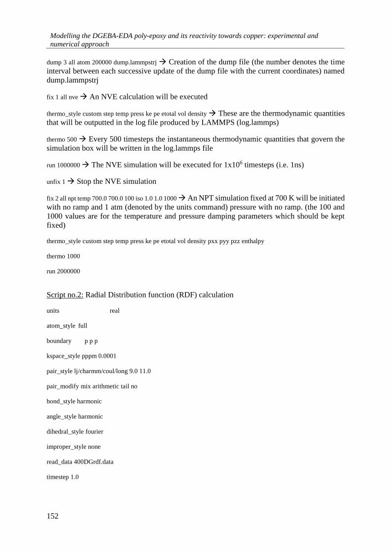
Modelling the DGEBA-EDA poly-epoxy and its reactivity towards copper: experimental and
numerical approach
152
dump 3 all atom 200000 dump.lammpstrj Creation of the dump file (the number denotes the time
interval between each successive update of the dump file with the current coordinates) named
dump.lammpstrj
fix 1 all nve An NVE calculation will be executed
thermo_style custom step temp press ke pe etotal vol density These are the thermodynamic quantities
that will be outputted in the log file produced by LAMMPS (log.lammps)
thermo 500 Every 500 timesteps the instantaneous thermodynamic quantities that govern the
simulation box will be written in the log.lammps file
run 1000000 The NVE simulation will be executed for 1x10⁶ timesteps (i.e. 1ns)
unfix 1 Stop the NVE simulation
fix 2 all npt temp 700.0 700.0 100 iso 1.0 1.0 1000 An NPT simulation fixed at 700 K will be initiated
with no ramp and 1 atm (denoted by the units command) pressure with no ramp. (the 100 and
1000 values are for the temperature and pressure damping parameters which should be kept
fixed)
thermo_style custom step temp press ke pe etotal vol density pxx pyy pzz enthalpy
thermo 1000
run 2000000
Script no.2: Radial Distribution function (RDF) calculation
units real
atom_style full
boundary p p p
kspace_style pppm 0.0001
pair_style lj/charmm/coul/long 9.0 11.0
pair_modify mix arithmetic tail no
bond_style harmonic
angle_style harmonic
dihedral_style fourier
improper_style none
read_data 400DGrdf.data
timestep 1.0
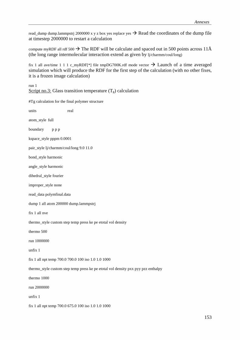
Annexes
153
read_dump dump.lammpstrj 2000000 x y z box yes replace yes Read the coordinates of the dump file
at timestep 2000000 to restart a calculation
compute myRDF all rdf 500 The RDF will be calculate and spaced out in 500 points across 11Å
(the long range intermolecular interaction extend as given by lj/charmm/coul/long)
fix 1 all ave/time 1 1 1 c_myRDF[*] file tmpDG700K.rdf mode vector Launch of a time averaged
simulation which will produce the RDF for the first step of the calculation (with no other fixes,
it is a frozen image calculation)
run 1
Script no.3: Glass transition temperature (Tg) calculation
#Tg calculation for the final polymer structure
units real
atom_style full
boundary p p p
kspace_style pppm 0.0001
pair_style lj/charmm/coul/long 9.0 11.0
bond_style harmonic
angle_style harmonic
dihedral_style fourier
improper_style none
read_data polymfinal.data
dump 1 all atom 200000 dump.lammpstrj
fix 1 all nve
thermo_style custom step temp press ke pe etotal vol density
thermo 500
run 1000000
unfix 1
fix 1 all npt temp 700.0 700.0 100 iso 1.0 1.0 1000
thermo_style custom step temp press ke pe etotal vol density pxx pyy pzz enthalpy
thermo 1000
run 2000000
unfix 1
fix 1 all npt temp 700.0 675.0 100 iso 1.0 1.0 1000

Modelling the DGEBA-EDA poly-epoxy and its reactivity towards copper: experimental and
numerical approach
154
thermo_style custom step temp press ke pe etotal vol density pxx pyy pzz enthalpy
thermo 1000
run 1000000
unfix 1
fix 1 all npt temp 675.0 650.0 100 iso 1.0 1.0 1000
thermo_style custom step temp press ke pe etotal vol density pxx pyy pzz enthalpy
thermo 1000
run 1000000
unfix 1
fix 1 all npt temp 650.0 625.0 100 iso 1.0 1.0 1000
thermo_style custom step temp press ke pe etotal vol density pxx pyy pzz enthalpy
thermo 1000
run 1000000
unfix 1
fix 1 all npt temp 625.0 600.0 100 iso 1.0 1.0 1000
thermo_style custom step temp press ke pe etotal vol density pxx pyy pzz enthalpy
thermo 1000
run 1000000
unfix 1
fix 1 all npt temp 600.0 575.0 100 iso 1.0 1.0 1000
thermo_style custom step temp press ke pe etotal vol density pxx pyy pzz enthalpy
thermo 1000
run 1000000
unfix 1
fix 1 all npt temp 575.0 550.0 100 iso 1.0 1.0 1000
thermo_style custom step temp press ke pe etotal vol density pxx pyy pzz enthalpy
thermo 1000
run 1000000
unfix 1

Annexes
155
fix 1 all npt temp 550.0 525.0 100 iso 1.0 1.0 1000
thermo_style custom step temp press ke pe etotal vol density pxx pyy pzz enthalpy
thermo 1000
run 1000000
unfix 1
fix 1 all npt temp 525.0 500.0 100 iso 1.0 1.0 1000
thermo_style custom step temp press ke pe etotal vol density pxx pyy pzz enthalpy
thermo 1000
run 1000000
unfix 1
fix 1 all npt temp 500.0 475.0 100 iso 1.0 1.0 1000
thermo_style custom step temp press ke pe etotal vol density pxx pyy pzz enthalpy
thermo 1000
run 1000000
unfix 1
fix 1 all npt temp 475.0 450.0 100 iso 1.0 1.0 1000
thermo_style custom step temp press ke pe etotal vol density pxx pyy pzz enthalpy
thermo 1000
run 1000000
unfix 1
fix 1 all npt temp 450.0 425.0 100 iso 1.0 1.0 1000
thermo_style custom step temp press ke pe etotal vol density pxx pyy pzz enthalpy
thermo 1000
run 1000000
unfix 1
fix 1 all npt temp 425.0 400.0 100 iso 1.0 1.0 1000
thermo_style custom step temp press ke pe etotal vol density pxx pyy pzz enthalpy
thermo 1000
run 1000000
unfix 1
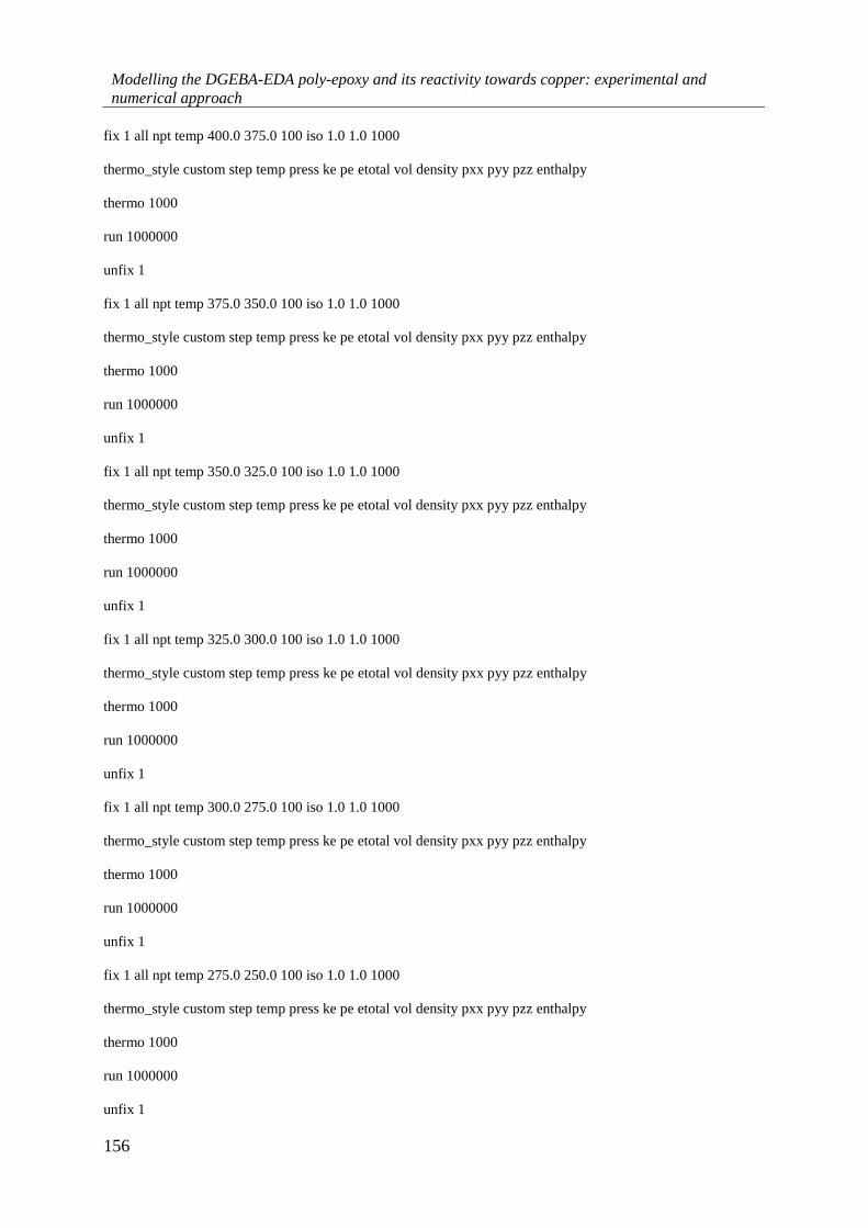
Modelling the DGEBA-EDA poly-epoxy and its reactivity towards copper: experimental and
numerical approach
156
fix 1 all npt temp 400.0 375.0 100 iso 1.0 1.0 1000
thermo_style custom step temp press ke pe etotal vol density pxx pyy pzz enthalpy
thermo 1000
run 1000000
unfix 1
fix 1 all npt temp 375.0 350.0 100 iso 1.0 1.0 1000
thermo_style custom step temp press ke pe etotal vol density pxx pyy pzz enthalpy
thermo 1000
run 1000000
unfix 1
fix 1 all npt temp 350.0 325.0 100 iso 1.0 1.0 1000
thermo_style custom step temp press ke pe etotal vol density pxx pyy pzz enthalpy
thermo 1000
run 1000000
unfix 1
fix 1 all npt temp 325.0 300.0 100 iso 1.0 1.0 1000
thermo_style custom step temp press ke pe etotal vol density pxx pyy pzz enthalpy
thermo 1000
run 1000000
unfix 1
fix 1 all npt temp 300.0 275.0 100 iso 1.0 1.0 1000
thermo_style custom step temp press ke pe etotal vol density pxx pyy pzz enthalpy
thermo 1000
run 1000000
unfix 1
fix 1 all npt temp 275.0 250.0 100 iso 1.0 1.0 1000
thermo_style custom step temp press ke pe etotal vol density pxx pyy pzz enthalpy
thermo 1000
run 1000000
unfix 1
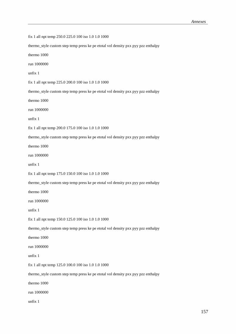
Annexes
157
fix 1 all npt temp 250.0 225.0 100 iso 1.0 1.0 1000
thermo_style custom step temp press ke pe etotal vol density pxx pyy pzz enthalpy
thermo 1000
run 1000000
unfix 1
fix 1 all npt temp 225.0 200.0 100 iso 1.0 1.0 1000
thermo_style custom step temp press ke pe etotal vol density pxx pyy pzz enthalpy
thermo 1000
run 1000000
unfix 1
fix 1 all npt temp 200.0 175.0 100 iso 1.0 1.0 1000
thermo_style custom step temp press ke pe etotal vol density pxx pyy pzz enthalpy
thermo 1000
run 1000000
unfix 1
fix 1 all npt temp 175.0 150.0 100 iso 1.0 1.0 1000
thermo_style custom step temp press ke pe etotal vol density pxx pyy pzz enthalpy
thermo 1000
run 1000000
unfix 1
fix 1 all npt temp 150.0 125.0 100 iso 1.0 1.0 1000
thermo_style custom step temp press ke pe etotal vol density pxx pyy pzz enthalpy
thermo 1000
run 1000000
unfix 1
fix 1 all npt temp 125.0 100.0 100 iso 1.0 1.0 1000
thermo_style custom step temp press ke pe etotal vol density pxx pyy pzz enthalpy
thermo 1000
run 1000000
unfix 1

Modelling the DGEBA-EDA poly-epoxy and its reactivity towards copper: experimental and
numerical approach
158
fix 1 all npt temp 100.0 75.0 100 iso 1.0 1.0 1000
thermo_style custom step temp press ke pe etotal vol density pxx pyy pzz enthalpy
thermo 1000
run 1000000
unfix 1
fix 1 all npt temp 75.0 50.0 100 iso 1.0 1.0 1000
thermo_style custom step temp press ke pe etotal vol density pxx pyy pzz enthalpy
thermo 1000
run 1000000
unfix 1
fix 1 all npt temp 50.0 25.0 100 iso 1.0 1.0 1000
thermo_style custom step temp press ke pe etotal vol density pxx pyy pzz enthalpy
thermo 1000
run 1000000
The above script uses consecutive NPT calculations that will diminish the initial temperature
of the NPT calculation (the first number after the temp keyword) to the final temperature (the
second number after the temp keyword) in the span of 1 ns given by the run parameter.
Bibliography
1. Plimpton, S. Fast Parallel Algorithms for Short-Range Molecular Dynamics. J. Comput.
Phys. 117, 1–19 (1995).
2. Hockney, R. & Eastwood, J. Particle-Particle-Particle-Mesh (P3M) Algorithms. in
Computer simulation using particles 267–304
3. Chapelle, O. & Erhan, D. Improved preconditioner for hessian free optimization. in In
NIPS Workshop on Deep Learning and Unsupervised Feature Learning (2011).

Annexes
159
Annex H: DGEBA simulation boxes and NPT simulation results for different
initial parameters
In this Annex we present results for the NPT simulations of pure DGEBA varying the initial
density and the number of molecules as well as the computational parameters. Unless stated
otherwise in the column “Other comments” the Particle Particle Particle Mesh (PPPM)
algorithm1 is used to calculate the intermolecular interactions and the GAFF force field2 is used
for the intramolecular parameters. The point charges we use are the ones calculated with the
RESP3,4 methodology.
Table 1. DGEBA NPT simulations under variable density, no. of molecules and computational
parameters
Test Number of
Molecules
T
(K)
ttot
(ns)
ρinitial
(g/cm3)
ρfinal
(g/cm3) Other comments
1 50 300 1 0.001 1.18 Pair_Style lj/cut/coul/cut
Rcut,lj = 5.0 Å, Rcut,coul = 3.0 Å
2 100 300 1 0.001 1.28 Pair_Style lj/cut/coul/cut
Rcut,lj = 5.0 Å, Rcut,coul = 3.0 Å
3 256 300 1 0.001 1.25 Pair_Style lj/cut/coul/cut
Rcut,lj = 5.0 Å, Rcut,coul = 3.0 Å
4 400 300 2 0.700 1.10
5 400 300 2 0.560 1.10
6 400 700 2 0.700 0.85
7 500 300 2 0.700 1.09
8 500 300 2 0.700 1.09
9 500 300 10 0.700 1.09
10 500 300 2 0.700 1.08 Pair_Style lj/cut/coul/cut
Rcut,lj = 9.0 Å, Rcut,coul = 9.0 Å
From Table 1 we can observe that for 400 DGEBA molecules, independent by the total
simulation time or the initial density, by using the same computational parameters for NPT
simulations at 300 K and 1 atm, the final density has a similar value around 1.09 g/cm3 which
is in good agreement with the experimental density of the liquid DGEBA5 at 300 K, i.e. 1.16
g/cm3. This value is lower if the temperature is increased at 700 K which is expected as the
volume expands more with an increase in the kinetic energy of the molecules. For 500 DGEBA

Modelling the DGEBA-EDA poly-epoxy and its reactivity towards copper: experimental and
numerical approach
160
molecules, using the same computational parameters for an NPT simulation fixed at 300 K and
1 atm, we calculate the same density as the 400 molecules. By changing the pair style to a style
that does not take into account the long range intermolecular interactions we have an
overestimation of the final density when the initial density is very low.
Bibliography
1. Hockney, R. & Eastwood, J. Particle-Particle-Particle-Mesh (P3M) Algorithms. in Computer
simulation using particles 267–304
2. Wang, J., Wolf, R. M., Caldwell, J. W., Kollman, P. A. & Case, D. A. Development and testing of
a general amber force field. J. Comput. Chem. 25, 1157–1174 (2004).
3. Bayly, C. I., Cieplak, P., Cornell, W. & Kollman, P. A. A well-behaved electrostatic potential based
method using charge restraints for deriving atomic charges: the RESP model. J. Phys. Chem. 97,
10269–10280 (1993).
4. Cornell, W. D., Cieplak, P., Bayly, C. I. & Kollmann, P. A. Application of RESP charges to
calculate conformational energies, hydrogen bond energies, and free energies of solvation. J. Am.
Chem. Soc. 115, 9620–9631 (1993).
5. DGEBA Epoxy Resin. Available at: http://polymerdatabase.com/polymers/bisphenol-
adiglycidyletherepoxyresin.html. (Accessed: 18th September 2017)

Annexes
161
Annex I: EDA simulation boxes and NPT simulation results for different initial
parameters
In this Annex we will present a variety of results using simulation boxes for the NPT
simulations pure EDA liquids varying the initial density and the number of molecules as well
as the computational parameters. Unless stated otherwise in the column “Other comments”
the Particle Particle Particle Mesh (PPPM) algorithm1 is used to calculate the intermolecular
interactions and the GAFF force field2 is used for the intramolecular parameters. The point
charges we use are the ones calculated with the RESP3,4 methodology.
Table 1. EDA NPT simulations tests under variable density, no. of molecules and computational
parameters
Test Number of
Molecules
T
(K)
ttot
(ns)
ρinitial
(g/cm3)
ρfinal
(g/cm3) Other comments
1 50 300 10 0.001 1.62 Pair_Style lj/cut/coul/cut
Rcut,lj = 5.0 Å, Rcut,coul = 3.0 Å
2 50 300 1 0.500 0.53 Pair_Style lj/cut/coul/cut
Rcut,lj = 5.0 Å, Rcut,coul = 3.0 Å
3 100 300 10 0.001 0.74 Pair_Style lj/cut/coul/cut
Rcut,lj = 5.0 Å, Rcut,coul = 3.0 Å
4 400 300 2 0.700 0.99
5 400 300 2 0.700 0.99
6 500 300 2 0.700 0.86
7 1000 300 1 0.700 0.96
From Table 1 we can observe that for 400 EDA molecules, for NPT simulations at 300 K and
1 atm, the final density has a value for all simulation boxes around 0.99 g/cm3 which is in a
fairly good accordance with the experimental value of 0.90 g/cm3 at 300 K5. This accordance
is improved if we use a 500 EDA molecule simulation box giving us a final density of 0.86
g/cm3. By changing the pair style to a style that does not take into account the long range
intermolecular interactions the final density in various conditions (from very low to higher
initial densities) is inconsistent and in the case of a 10 ns simulation is dramatically increased
to a value of 1.62 g/cm3 suggesting that for a longer simulation the box could explode as a very
small volume would create very large energies crashing the simulation. . This shows us that a
computational method not taking into account long range effects will not yield the desirable
results and is abandoned.

Modelling the DGEBA-EDA poly-epoxy and its reactivity towards copper: experimental and
numerical approach
162
Bibliography
1. Hockney, R. & Eastwood, J. Particle-Particle-Particle-Mesh (P3M) Algorithms. in Computer
simulation using particles 267–304
2. Wang, J., Wolf, R. M., Caldwell, J. W., Kollman, P. A. & Case, D. A. Development and testing of
a general amber force field. J. Comput. Chem. 25, 1157–1174 (2004).
3. Bayly, C. I., Cieplak, P., Cornell, W. & Kollman, P. A. A well-behaved electrostatic potential based
method using charge restraints for deriving atomic charges: the RESP model. J. Phys. Chem. 97,
10269–10280 (1993).
4. Cornell, W. D., Cieplak, P., Bayly, C. I. & Kollmann, P. A. Application of RESP charges to
calculate conformational energies, hydrogen bond energies, and free energies of solvation. J. Am.
Chem. Soc. 115, 9620–9631 (1993).
5. Ethylenediamine E26266. NH2CH2CH2NH2 Available at:
http://www.sigmaaldrich.com/catalog/product/sial/e26266. (Accessed: 18th September 2017)

Annexes
163
Annex J: Test of several temperatures for NPT simulations of the DGEBA, EDA
and stoichiometric mixture simulation boxes
This Annex includes NPT simulations at higher temperatures for the DGEBA and EDA
reactants and their stoichiometric mixture. These NPT simulations are used to study the
behavior of such simulation boxes at higher temperatures. Higher temperatures allow the
vigorous motion of molecules. In the mixture, it allows a better distribution of the molecules
inside the simulation box, potentially allowing more reactive centers to be cross-linked. We
tested NPT simulations fixed at 700 K and 1 atm for the DGEBA and EDA reactants. For the
stoichiometric mixture we tested two fixed temperatures (900 K and 1000 K) and a fixed 1 atm
pressure. The results are presented in Figures 1-4. For all the simulation boxes the initial density
was fixed at 0.700 g/cm3.
Figure 1. 2ns NPT simulation of the 400 DGEBA monomer box fixed at 700 K and 1 atm.
Figure 1a presents the variation of the temperature as a function of time. We observe that the
temperature is well equilibrated throughout the simulation duration around the value that we
have fixed with the thermostat (700 K). The oscillations are in a limited range of ± 6 K which
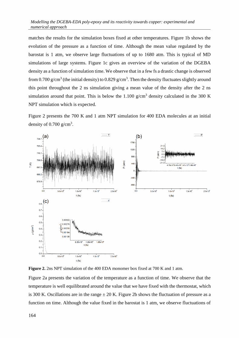
Modelling the DGEBA-EDA poly-epoxy and its reactivity towards copper: experimental and
numerical approach
164
matches the results for the simulation boxes fixed at other temperatures. Figure 1b shows the
evolution of the pressure as a function of time. Although the mean value regulated by the
barostat is 1 atm, we observe large fluctuations of up to 1680 atm. This is typical of MD
simulations of large systems. Figure 1c gives an overview of the variation of the DGEBA
density as a function of simulation time. We observe that in a few fs a drastic change is observed
from 0.700 g/cm3 (the initial density) to 0.829 g/cm3. Then the density fluctuates slightly around
this point throughout the 2 ns simulation giving a mean value of the density after the 2 ns
simulation around that point. This is below the 1.100 g/cm3 density calculated in the 300 K
NPT simulation which is expected.
Figure 2 presents the 700 K and 1 atm NPT simulation for 400 EDA molecules at an initial
density of 0.700 g/cm3.
Figure 2. 2ns NPT simulation of the 400 EDA monomer box fixed at 700 K and 1 atm.
Figure 2a presents the variation of the temperature as a function of time. We observe that the
temperature is well equilibrated around the value that we have fixed with the thermostat, which
is 300 K. Oscillations are in the range ± 20 K. Figure 2b shows the fluctuation of pressure as a
function on time. Although the value fixed in the barostat is 1 atm, we observe fluctuations of
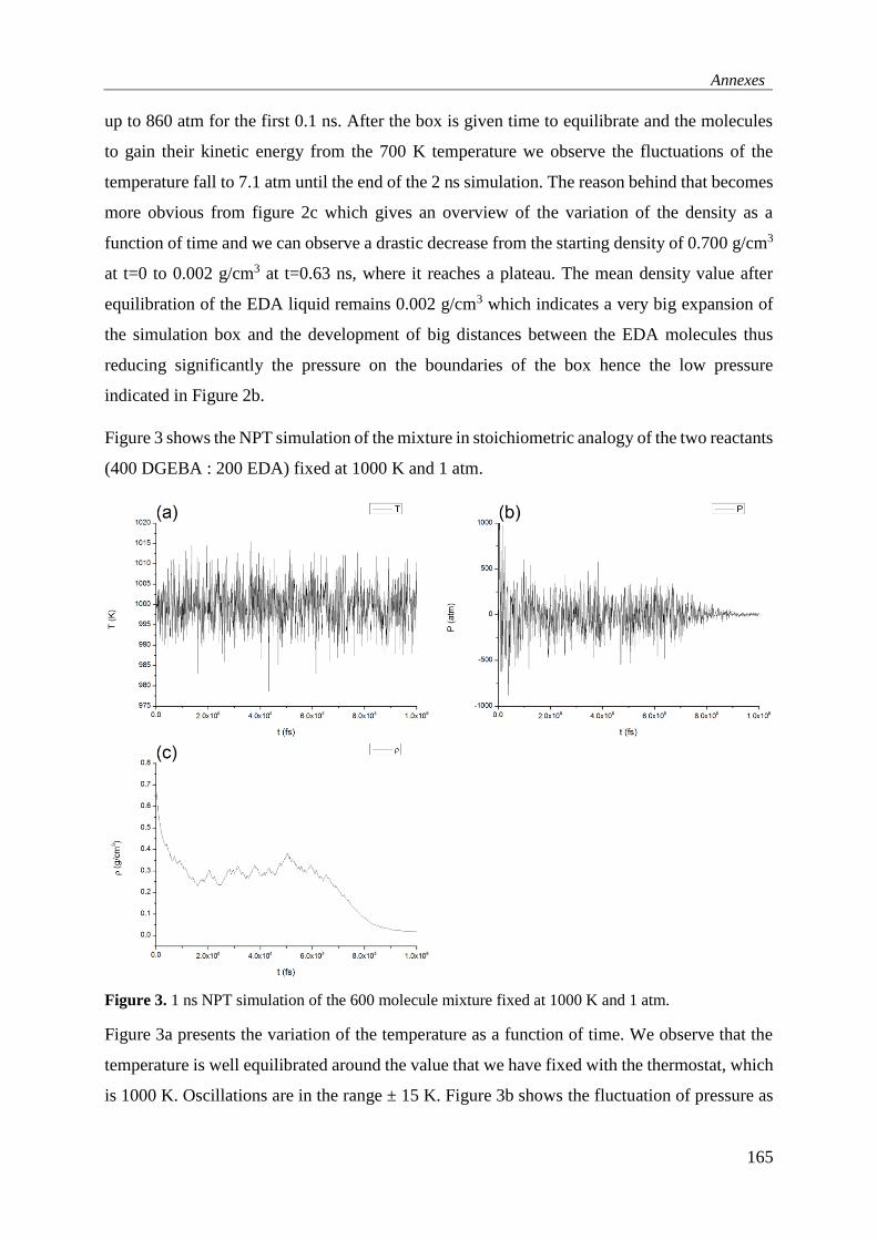
Annexes
165
up to 860 atm for the first 0.1 ns. After the box is given time to equilibrate and the molecules
to gain their kinetic energy from the 700 K temperature we observe the fluctuations of the
temperature fall to 7.1 atm until the end of the 2 ns simulation. The reason behind that becomes
more obvious from figure 2c which gives an overview of the variation of the density as a
function of time and we can observe a drastic decrease from the starting density of 0.700 g/cm3
at t=0 to 0.002 g/cm3 at t=0.63 ns, where it reaches a plateau. The mean density value after
equilibration of the EDA liquid remains 0.002 g/cm3 which indicates a very big expansion of
the simulation box and the development of big distances between the EDA molecules thus
reducing significantly the pressure on the boundaries of the box hence the low pressure
indicated in Figure 2b.
Figure 3 shows the NPT simulation of the mixture in stoichiometric analogy of the two reactants
(400 DGEBA : 200 EDA) fixed at 1000 K and 1 atm.
Figure 3. 1 ns NPT simulation of the 600 molecule mixture fixed at 1000 K and 1 atm.
Figure 3a presents the variation of the temperature as a function of time. We observe that the
temperature is well equilibrated around the value that we have fixed with the thermostat, which
is 1000 K. Oscillations are in the range ± 15 K. Figure 3b shows the fluctuation of pressure as

Modelling the DGEBA-EDA poly-epoxy and its reactivity towards copper: experimental and
numerical approach
166
a function on time. Although the value fixed in the barostat is 1 atm, we observe fluctuations
of up to 500 atm for the first 0.8 ns. After the box is given time to equilibrate and the molecules
to gain their kinetic energy from the 1000 K temperature we observe the fluctuations of the
temperature fall to 20 atm until the end of the 1 ns simulation. The reason behind that becomes
more obvious from Figure 3c which gives an overview of the variation of the density as a
function of time and we can observe a drastic decrease from the starting density of 0.700 g/cm3
at t=0 to 0.250 g/cm3 that indicates the rapid movement and thus distancing of the molecules
leading to a rapid expansion of the simulation box. This density has oscillations in the range of
±0.1 g/cm3 until t=0.7ns where it steadily descends at 0.002 g/cm3 at t=0.80 ns, where it reaches
a plateau. The oscillations are a result of the DGEBA molecules not being able to reach a kinetic
energy high enough for them to escape their attractive forces. The mean density value after
equilibration of the stoichiometric molecular mixture remains 0.002 g/cm3 which indicates a
very big expansion of the simulation box and the development of big distances between the
largest (DGEBA) molecules thus reducing significantly the pressure on the boundaries of the
box hence the low pressure indicated in Figure 3b.
Figure 4 shows the NPT simulation of the mixture in stoichiometric analogy of the two reactants
fixed at 900 K and 1 atm.
Figure 4. 1 ns NPT simulation of the 600 molecule mixture fixed at 900 K and 1 atm.

Annexes
167
Figure 4a presents the variation of the temperature as a function of time. We observe that the
temperature is well equilibrated throughout the simulation duration around the value that we
have fixed with the thermostat (900 K). The oscillations are again as with the 1000 K NPT
simulation in the range of ± 15 K. Figure 4b shows the evolution of the pressure as a function
of time. Although the mean value regulated by the barostat is 1 atm, we observe large
fluctuations of up to 740 atm throughout the 2ns simulation. Figure 4c gives an overview of the
variation of the density as a function of simulation time. We observe that in a few fs a drastic
change is observed from 0.700 g/cm3 to 0.522 g/cm3. Then the density fluctuates slightly around
this point throughout the 2 ns simulation giving a mean value of the density after the 2 ns
simulation around that point. We can thus deduce that a 900 K temperature allows the molecules
to move in the simulation box vigorously but does not provide too much kinetic energy to
escape as it was the case at 1000 K (ρfinal ~ 0.002 g/cm3). Thus we conclude that if a higher
temperature is to be tested for the cross-linking algorithm, 900 K or below should be considered.
Bibliography
1. Landau, L. D. & Lifshitz, E. M. Statistical Physics. (Pergamon Press).


Résumé vulgarisé en français
Il y a un besoin croissant de substituer certains composants métalliques utilisés dans les
industries de l'aérospatiale et du transport, par des matériaux plus légers. Dans cette optique,
les polymères (la famille comprenant les plastiques) sont de bons candidats. Mais leurs
propriétés physiques et chimiques sont totalement différentes de celles des métaux. Par
exemple, certains composants doivent pouvoir conduire l'électricité. Les pièces métalliques le
font mais les plastiques sont des isolants électriques. Dans ce cas, une couche de métal peut être
déposée sur la surface du composant polymère. De nombreuses techniques ont été développées
pour la métallisation des polymères, mais aucune n'est universelle. Par conséquent, il est
nécessaire d'élaborer des modèles qui pourraient être utiles à la compréhension de l’élaboration
de la majorité des systèmes métal / polymère. Dans cet objectif, nous avons développé une
méthodologie scientifique capable d'identifier et d'expliquer les processus responsables de la
formation de la couche de métallisation sur la surface du polymère. Ce modèle est basé sur la
combinaison de simulations informatiques et de travaux expérimentaux. Afin de comprendre
en détails la formation d'une couche de cuivre sur un polymère utilisé dans l'industrie
aérospatiale, nous avons construit un modèle numérique de ce polymère qui sera très utile pour
d'autres études scientifiques.
Popularized summary in English
There is a growing interest in the substitution of metallic components used in the aerospace and
transport industries, by lighter materials. Polymers (the family of plastics) are good candidates
in this purpose. But their physical and chemical properties are totally different. For instance,
some components need to conduct electricity. Metallic parts do; plastics don’t. In these cases,
a metallization layer is requested over the polymer component surface. Many techniques were
developed for metallizing polymers, but none is universal. Therefore, there is a need to develop
models which could be useful to the understanding of the majority of metal/polymer systems.
In this course, we have developed a scientific methodology which is able to identify and explain
the processes that are responsible for the formation of the metallization layer on the polymer
surface. It is based on the combination of computational simulations and experimental work.
At the end, we could explain better the formation of a copper layer on a polymer used in the
aerospace industry, and we developed a numerical model of this polymer that will be very useful
for further studies.


Titre. Modélisation du poly-époxy DGEBA-EDA et de sa réactivité vis à vis du cuivre : approche expérimentale et numérique
Résumé. Grâce à la métallisation de leur surface, des pièces en polymères peuvent substituer certains composants métalliques dans
les industries de l'aérospatiale et du transport. Les polymères ont des masses volumiques plus faibles que les métaux et une réactivité
chimique limitée, ce qui en fait des candidats idéaux pour les applications spatiales. En combinant techniques expérimentales et
simulations numériques, nous avons étudié les mécanismes fondamentaux de la métallisation de surface d'un polymère poly-époxy
(DGEBA / EDA). L'objectif de notre étude était de développer un modèle non empirique prenant en compte les mécanismes régissant
la nucléation et la croissance des films minces métalliques. Notre groupe a une longue expérience des dépôts chimiques en phase
vapeur, CVD. Mais cette technique n’a pas été choisie pour la métallisation de nos surfaces de polymères car les températures requises
dans le réacteur étaient trop élevées. Comme alternative, nous avons effectué une évaporation sous ultravide de Cu à température
ambiante, conduisant à une diffusion des atomes en phase gazeuse sans énergie cinétique. Les processus d'adsorption et de diffusion
sont donc plus proches des conditions thermodynamiques associées aux calculs. Un protocole expérimental a été mis en place afin de
créer une surface polymère chimiquement homogène présentant une faible rugosité. Le polymère obtenu a été caractérisé (i) par
spectroscopie infrarouge à transformée de Fourier, pour déterminer le taux de polymérisation (supérieur à 90%), (ii) par calorimétrie
différentielle à balayage pour obtenir la température de transition vitreuse (Tg) ( 118,1 °C), (iii) par microscopie à force atomique
(AFM) pour estimer la rugosité de la surface (Ra ≈ 1 nm), et (iv) par spectroscopie de photoélectrons X (XPS) pour caractériser les
liaisons chimiques de surface. La surface de polymère a ensuite été métallisée. Grâce à des analyses AFM, l'épaisseur du film mince
a été estimée à 6 nm. Nous avons ensuite utilisé l’XPS pour caractériser les liaisons interfaciales Cu / Poly-époxy. Nous avons déduit
de l’interprétation des spectres XPS que le Cu est adsorbé préférentiellement sur un atome d'oxygène spécifique du polymère. Pour
identifier clairement ces sites d'adsorption de Cu, nous avons ensuite simulé les spectres XPS du polymère non revêtu, par des calculs
quantiques, en utilisant un modèle moléculaire (dimère : 1 molécule de DGEBA liée à 1 molécule d'EDA). Les méthodes Hartree-
Fock (HF) et de la théorie de la fonctionnelle de la densité (DFT) nous ont permis de simuler des spectres XPS pour la surface nue,
en prenant en compte les effets d’état final et initial. Grâce à ces résultats, nous avons pu décomposer le spectre expérimental en 8
contributions, ce qui conduit à des résultats beaucoup plus précis que les résultats habituels obtenus par l'utilisation exclusive des
expériences et de la littérature. Nous avons ensuite effectué des simulations de dynamique moléculaire classique (MD) pour passer
d'un modèle moléculaire (dimère) à un modèle de polymère amorphe. Nous avons utilisé le champ de force Amber généralisé (GAFF)
et nous avons développé un code de réticulation des molécules de monomères. Le système initial était un mélange stœchiométrique
de molécules DGEBA et EDA qui a été équilibré à 700K. Lorsque l'équilibre a été atteint, certaines propriétés structurales (par
exemple, la distribution des liaisons) ont été extraites des simulations NPT. À partir de ce mélange liquide de monomères, notre code
de réticulation a identifié et relié les atomes réactifs (à une distance interatomique prédéfinie < 3 Å). Après chaque étape de
polymérisation, le système a été rééquilibré à 700K (simulations NPT). Après plusieurs cycles de réticulation/simulation de dynamique
moléculaire, nous avons pu atteindre un taux de polymérisation de 93% et la fonction de distribution radiale (RDF), la masse
volumique (1.115 à 300K) et la température de transition vitreuse Tg (115,5 °C) ont été calculées. La Tg est en accord avec la valeur
expérimentale de 118,1 °C, validant notre approche numérique pour développer un modèle pour les polymères poly-époxy.
Title. Modelling the DGEBA-EDA poly-epoxy and its reactivity towards copper: experimental and numerical approach
Abstract. Metallization of polymer surfaces can lead to the substitution of metallic components. Polymers have lower densities and
limited chemical reactivity, making them ideal candidates for the space applications. Through experiments and calculations, we
studied the fundamental mechanisms of surface metallization of a poly-epoxy polymer (DGEBA/EDA). The objective of our study
was to develop a non-empirical model that could take into account the mechanisms governing the nucleation and growth of thin metal
films. Our group has a long experience in chemical vapor deposition, CVD, and metallization of polymer composites. But we did not
applied CVD at first because of the high temperatures required in the reactor. We alternatively used ultrahigh vacuum evaporation of
Cu at ambient temperature. Therefore, we make sure that atoms diffuse in the gas phase without kinetic energy. Adsorption and
diffusion processes are thus closer to thermodynamic conditions that prevails in calculations. An experimental protocol was refined
in order to create a chemically homogeneous polymer surface with a low roughness (Ra<1nm). The bulk and the surface of the pristine
polymer were characterized (i) by Fourier Transform Infrared Spectroscopy, to determine the polymerization rate (above 90%), (ii)
by differential scanning calorimetry in order to obtain the glass transition temperature (Tg) (118.1 °C), (iii) by atomic force microscopy
(AFM) to calculate surface roughness (Ra ≈ 1 nm), and (iv) by X-ray photoelectron spectroscopy (XPS) to characterize surface
chemical bonding. The surface was then metallized. Through AFM, the thickness of the thin film was estimated at 6 nm. We then
used XPS to characterize the Cu/Poly-epoxy interfacial bonding. We deduced that Cu adsorbed preferentially on a specific oxygen
atom of the polymer. To clearly identify this Cu adsorption site, we further simulated the XPS spectra of our clean or metallized
polymer by quantum calculations, using a dimer model (1 molecule of DGEBA connected to 1 molecule of EDA). In the Hartree-
Fock (HF) and Density Functional Theory (DFT) framework, we first simulated the XPS spectra for the pristine surface taking into
account initial and final state effects. Thanks to these results, we were able to analyze the experimental spectrum with 8 contributions,
leading to much more accurate results than the usual results obtained by the exclusive use of experiments and literature. We then
performed classical Molecular Dynamics (MD) simulations to move from a dimer model to an amorphous polymer model. We used
the general Amber force field (GAFF) and we developed a code to mimic the reticulation of monomers molecules. We started from a
stoichiometric mixture of DGEBA and EDA molecules. When equilibration was reached, structural properties at 700K (e.g.
distribution of bonds) were extracted from the results of the NPT simulations. From this melt of monomers, the homemade reticulation
code identified and connected reactive atoms (at a pre-defined inter-atomic distance < 3Å). After each step of polymerization, the
system was equilibrated at 700K (NPT simulations). After multiple reticulation/MD cycles we could achieve a polymerization rate of
93% and the Radial Distribution Function (RDF), the density and the glass transition temperature Tg were calculated. The value of the
computed density was 1.115 at 300K and the calculated Tg (115.5 °C) was in good agreement with the experimental Tg of 118.1 °C,
validating our numerical approach to develop a model for poly-epoxies.