Modelling Stress Relaxation in Bolt Loaded...

Modelling Stress Relaxation in BoltLoaded CT–SpecimensMaster’s Thesis in Nuclear Engineering

Shervin Shojaee

Department of Applied PhysicsDivision of Nuclear EngineeringChalmers University of TechnologyGothenburg, Sweden 2014CTH-NT-297

ISSN 1653-4662

REPORT NO. CTH-NT-297/ISSN 1653-4662

Modelling Stress Relaxation in BoltLoaded CT–Specimens

A Thesis Submitted in Partial Fulfilment of the Requirements for the Degree of

Master of Science in Nuclear Engineering

Shervin Shojaee

Department of Applied PhysicsDivision of Nuclear Engineering

Chalmers University of TechnologyGothenburg, Sweden 2014

Modelling Stress Relaxation in Bolt Loaded CT–SpecimensMaster’s Degree Thesis in Nuclear EngineeringShervin Shojaee

c© Shervin Shojaee, 2014.

Technical report no. CTH-NT-297/ISSN 1653-4662Department of Applied PhysicsDivision of Nuclear EngineeringChalmers University of TechnologySE–412 96 GothenburgSwedenTelephone +46 (0)31-772 1000

Cover:A bolt loaded CT-specimen.

Chalmers ReproserviceGothenburg, Sweden 2014

Modelling Stress Relaxation in Bolt Loaded CT–SpecimensMaster’s Degree Thesis in Nuclear EngineeringShervin ShojaeeDepartment of Applied PhysicsDivision of Nuclear EngineeringChalmers University of Technology

Abstract

Cracks in welds at higher temperature ranges (288 ◦C) are prone to creep deformation andhence affect the crack tip stresses. Various creep models are presented. One of the modelsare used to describe the bolt load relaxation of modified CT-specimens analytically. Themodel is compared to numerical results using Ansys. The long term bolt load relaxationrate described by the model was similar to the three dimensional numerical analysis.

It should be noted that a performed experimental bolt load relaxing experiment wasperformed, but due to lack of creep deformation data at the temperature of interest,fictive material data parameters were used instead. The CT-specimen was bolt loadedwith 16.66 kN. After a 50 h heat treatment cycle at 288 ◦C, the bolt had relaxed byapproximately 30 %.

A bolt load relaxation model for fictive materials were compared with numericalresults using the numerical calculation tool Ansys. The shape of the model was consistentwith the numerical results, although, some calibrations of the model is still required toreach a satisfying result.

Keywords: CT-specimen, Steady state cracks, Viscoelasticity, Rheology, Creep models,Norton’s creep law, Stress relaxation, Stress intensity factor, Numerical analysis.

To my family

Contents

List of Figures x

List of Tables xi

Acknowledgements xii

Introduction xiii

List of Abbreviations xvi

List of Symbols xviii

1 Mechanics of Materials 11.1 Material structure . . . . . . . . . . . . . . . . . . . . . . . . . . . . . . . . 1

1.1.1 Atomic structures . . . . . . . . . . . . . . . . . . . . . . . . . . . . 1

1.2 Material behaviour . . . . . . . . . . . . . . . . . . . . . . . . . . . . . . . . 6

1.2.1 Hooke’s law and Hooke’s generalised law . . . . . . . . . . . . . . . . 9

1.2.2 Elasticity, plasticity and viscoelasticity . . . . . . . . . . . . . . . . . 11

1.2.3 Creep deformation . . . . . . . . . . . . . . . . . . . . . . . . . . . . 12

1.2.4 Stress relaxation . . . . . . . . . . . . . . . . . . . . . . . . . . . . . 13

1.3 Cracks . . . . . . . . . . . . . . . . . . . . . . . . . . . . . . . . . . . . . . 14

1.3.1 Stresses near a crack tip . . . . . . . . . . . . . . . . . . . . . . . . 14

1.3.2 Loading modes . . . . . . . . . . . . . . . . . . . . . . . . . . . . . 15

1.3.3 Irwin plastic correction approach . . . . . . . . . . . . . . . . . . . . 17

1.4 Numerical computational calculations . . . . . . . . . . . . . . . . . . . . . 19

1.4.1 Finite element method . . . . . . . . . . . . . . . . . . . . . . . . . 19

2 Methodology 242.1 Experiment . . . . . . . . . . . . . . . . . . . . . . . . . . . . . . . . . . . . 24

2.1.1 Manufacturing the CT-specimens . . . . . . . . . . . . . . . . . . . . 24

2.1.2 Crack initiation . . . . . . . . . . . . . . . . . . . . . . . . . . . . . 25

2.1.3 Bolt loading . . . . . . . . . . . . . . . . . . . . . . . . . . . . . . . 25

vii

viii Contents

2.1.4 Heat treatment . . . . . . . . . . . . . . . . . . . . . . . . . . . . . 252.1.5 Measuring bolt tension . . . . . . . . . . . . . . . . . . . . . . . . . 25

2.2 Rheological models . . . . . . . . . . . . . . . . . . . . . . . . . . . . . . . 262.2.1 Maxwell model . . . . . . . . . . . . . . . . . . . . . . . . . . . . . 272.2.2 Standard linear solid model . . . . . . . . . . . . . . . . . . . . . . . 282.2.3 Generalised Maxwell model . . . . . . . . . . . . . . . . . . . . . . . 292.2.4 Norton model . . . . . . . . . . . . . . . . . . . . . . . . . . . . . . 312.2.5 Bolt relaxation based on Norton’s stress relaxation model . . . . . . . 31

3 Results 343.1 Numerical analysis using Ansys . . . . . . . . . . . . . . . . . . . . . . . . . 34

3.1.1 Geometry . . . . . . . . . . . . . . . . . . . . . . . . . . . . . . . . 343.1.2 Input data . . . . . . . . . . . . . . . . . . . . . . . . . . . . . . . . 343.1.3 Meshing . . . . . . . . . . . . . . . . . . . . . . . . . . . . . . . . . 363.1.4 Bolt pretension . . . . . . . . . . . . . . . . . . . . . . . . . . . . . 373.1.5 Ansys results . . . . . . . . . . . . . . . . . . . . . . . . . . . . . . . 38

3.2 Comparison of theoretical models to numerical FEM calculation results . . . 43

4 Conclusions 454.1 Remarks about the theoretical results . . . . . . . . . . . . . . . . . . . . . . 454.2 Remarks about the numerical FEM-calculation results . . . . . . . . . . . . . 464.3 Future work . . . . . . . . . . . . . . . . . . . . . . . . . . . . . . . . . . . 46

Bibliography 49

Appendices 51

A Drawing 3003329 Revision 2 53

B Drawing 1090900 Revision 03 55

List of Figures

1.1.1 Lattice structures . . . . . . . . . . . . . . . . . . . . . . . . . . . . . . . . 2

1.1.2 Salt – NaCl . . . . . . . . . . . . . . . . . . . . . . . . . . . . . . . . . . . 2

1.1.3 Polycrystalline lattice formation . . . . . . . . . . . . . . . . . . . . . . . . . 3

1.1.4 The L-J potential . . . . . . . . . . . . . . . . . . . . . . . . . . . . . . . . 4

1.1.5 The Frenkel and Schottky defects . . . . . . . . . . . . . . . . . . . . . . . . 4

1.1.6 Edge dislocation structure and motion . . . . . . . . . . . . . . . . . . . . . 6

1.2.1 Applied forces P on a rod with cross-sectional area A′ . . . . . . . . . . . . 7

1.2.2 Applied forces P on a rod with the elongation δ . . . . . . . . . . . . . . . . 7

1.2.3 Applied forces P on a rod with cross-sectional area A′ . . . . . . . . . . . . 8

1.2.4 Applied forces P on the surface of a rectangular block . . . . . . . . . . . . 8

1.2.5 A bilinear material behaviour with yield stress marked . . . . . . . . . . . . . 9

1.2.6 A typical creep behaviour and the name of its different states . . . . . . . . . 13

1.3.1 A elliptic shaped crack inside a large specie . . . . . . . . . . . . . . . . . . 15

1.3.2 The stresses in an infinitesimal volume near the crack tip . . . . . . . . . . . 15

1.3.3 Three different loading modes . . . . . . . . . . . . . . . . . . . . . . . . . 16

1.3.4 The stresses near the crack tip . . . . . . . . . . . . . . . . . . . . . . . . . 16

1.3.5 The standardised CT-specimen with dimensions . . . . . . . . . . . . . . . . 18

1.3.6 A schematic figure of Irwin iteration process . . . . . . . . . . . . . . . . . . 19

1.4.1 Two dimensional wlement with 8 nodes . . . . . . . . . . . . . . . . . . . . 20

1.4.2 Linear and quadratic elements . . . . . . . . . . . . . . . . . . . . . . . . . 21

1.4.3 Mesh design around the crack tip . . . . . . . . . . . . . . . . . . . . . . . . 23

2.2.1 Rheological components (spring and dash-pot) . . . . . . . . . . . . . . . . . 26

2.2.2 The rheological Maxwell model . . . . . . . . . . . . . . . . . . . . . . . . . 27

2.2.3 The rheological SLS-model . . . . . . . . . . . . . . . . . . . . . . . . . . . 28

2.2.4 The rheological general Maxwell model . . . . . . . . . . . . . . . . . . . . . 30

2.2.5 The rheological Norton model . . . . . . . . . . . . . . . . . . . . . . . . . . 31

2.2.6 Load relaxation models with two fictive material . . . . . . . . . . . . . . . . 33

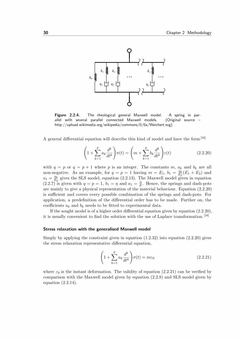
3.1.1 The geometries used for the numerical FEM-calculations . . . . . . . . . . . 35

3.1.2 The assembled bolt and CT-specimen . . . . . . . . . . . . . . . . . . . . . 36

ix

x List of Figures

3.1.3 Smaller mesh elements in front of the crack tip . . . . . . . . . . . . . . . . 373.1.4 Crack tip mesh . . . . . . . . . . . . . . . . . . . . . . . . . . . . . . . . . 383.1.5 Linear elastic results (case 1) from numerical FEM-calculations . . . . . . . . 393.1.6 Stress intensity factor along the crack edge for case 1 . . . . . . . . . . . . . 403.1.7 Stress and deformation results for for case 2 . . . . . . . . . . . . . . . . . . 413.1.8 Stress and deformation results for for case 3 . . . . . . . . . . . . . . . . . . 423.1.9 Stress and deformation results for for case 4 . . . . . . . . . . . . . . . . . . 423.2.1 Bolt load relaxation model and FEM-calculation (case 3 and 4) . . . . . . . . 443.2.2 Bolt load relaxation model and FEM-calculation (case 2) . . . . . . . . . . . 44

List of Tables

1.3.1 The functions f(I)ij for i, j ∈ {x, y, z} . . . . . . . . . . . . . . . . . . . . . . 17

2.1.1 Measured experimental bolt loads values . . . . . . . . . . . . . . . . . . . . 262.2.1 Material data and Norton parameters . . . . . . . . . . . . . . . . . . . . . . 32

3.1.1 Bolt material and Norton parameters . . . . . . . . . . . . . . . . . . . . . . 363.1.2 Ct-specimen material and Norton parameters . . . . . . . . . . . . . . . . . 37

xi

Acknowledgements

I would like to express my greatest gratitude to Pal Efsing, Bjorn Forsgren, MartinBerglund and Johan Haglund for their help and support regarding theories of fracturemechanics, FEM-calculations and proof reading. Patrik Andersson is also greatly acknowl-edged, together with AF and Vattenfall, for making this master’s thesis project possible.Examiner Anders Nordlund, the head of the nuclear engineering master’s programme atthe Chalmers University of Technology, have my humblest appreciation for his remarksand possible improvements of the report as well as for his commitment to the master’sprogramme.

Shervin Shojaee, Gothenburg 2014/05/16.

xii

Introduction

This report will be introduced with some background information and purpose of thework. It will further be motivated by the reason of its value. The main result of thework lies around a load relaxation model in bolt load modified Compact Tension (CT)specimens [1] which was compared to three dimensional numerical results using Ansys.

Background

Nuclear Power Plants

One of the most essential component in a nuclear power plant (NPP) is the complexpiping system. These pipes are exposed to extreme environments in terms of temperature,pressures and chemical interactions. In addition to this, ionising radiation is also present inthe most vital parts. The harsh environment make the components prone to developmentof defects and cracks which eventually leads to fractures if not replaced or repaired. Asthe safety of a NPP is the highest priority, the understanding of the crack developmentand crack growth is an essential knowledge of structural integrity of the components.

Crack growth

A substantial portion of the experimental stress corrosion crack growth data for theSwedish nuclear power plant industries have been generated in the autoclaves at Os-karshamn reactor 2 and 3, as well as in hydrogen water chemistry (HWC) and normalwater chemistry (NWC) environments. In these experiments, the CT-specimens can beexposed during longer periods of time resulting in an opportunity to model long termbehaviours of the stress corrosion cracking. Unfortunately, there are no unambiguousstandards to follow for this type of stress corrosion cracking tests regarding the choiceof specimens. Considering the standards ASTM E647 [2] used for fatigue testing andASTM E1820 [3] used for fracture mechanics testing, the CT-specimen for this experimentseems a reasonable choice.

With a valid model describing the crack growth over time in these environments, itis possible to foresee when defects reach a critical size. Hence, cyclic inspections can

xiii

xiv Introduction

be established from the models to provide a cost effective and safe maintenance of thereactors.

Generally in fracture mechanics, crack growth follows the Paris law (or some variantof it) [4–6]

dacdN

= Ac(∆K)s,

where ac is the crack length, N the number of load cycles affecting the crack and K thestress intensity factor describing the crack state, which differs for different geometriesand loads. As the cyclic loads change from a maximum to a minimum stress intensityfactor, ∆K denotes the range of change of the stress intensity factor during the cyclicload. The Ac and s parameters are material dependent.

At most cases, if not always, the avoidance of stress corrosion cracking is the highestpriority. The materials’ resistance to stress corrosion cracking deviates with dependenceon the alloy in use and the environmental influence upon it. Additionally, the structuralintegrity of any component has to be designed to withstand applied forces, environmentalinfluences, temperature changes and also be economical sustainable in a long termperspective. Nevertheless, stress corrosion cracks in the harsh NPP environments cannot be eluded and must therefore be considered when designing a component.

It has been noticed that experimental crack growth data does not meet earlierpredictions and it is believed that the creep deformation and stress relaxations influenceson the crack front stresses can not be omitted as was earlier assumed reasonable. [7] Bymaking a material creep until the creep behaviour is not longer noticed, the residualstresses can be assumed to be no longer existent (it is most probably the variationof the residual stresses in earlier specimens that gave large variations in the previousmeasurements). Therefore, it is highly convenient to know for how long a material needsto be exposed to creep deformation until no longer detectable.

Bolt load relaxation experiment

Generally, CT-specimens are applied with active loads in a laboratory environment.Active loads are simply the case when a specie is applied with controlled loads. They arecontrolled by the tensions of the species, at all times, being adjusted to reach a specificmagnitude of force. The testing of this kind is expensive for time consuming experiments,due to the species occupying advanced and expensive equipments. Hence, a modificationof the CT-specimens are made for the ability to use passive loads. A passive load is aninitially applied load which is not adjusted for the variation over time. In this case, thepassive loads are comprised by bolt loading the CT-specimens. The modification wasused in an experiment performed by Royal Institute of Technology (KTH) in Sweden.The experiment involved the bolt load relaxation at an elevated temperature1 (288 ◦C).

1 Elevated temperature relative the room temperature.

Introduction xv

Purpose

The work in this report involves the analysis of the collected data from the performedexperiment by KTH and to determine whether a valid model of the bolt load relaxationin these environments can be found.

Objective

The project consists of an investigation to determine if there exists analytical models todescribe the stress relaxation based on the collected data. As no material data describingthe material behaviour could be found, fictional parameters were used and the modelwere then compared to three dimensional numerical simulations of the specimens.

Scope

Four pre-existing models were investigated. These models are presented. A self derivedbolt relaxation model was developed from one of the stress relaxation models andundergoes validation against the numerical simulation of the transient. A finite elementmethod (FEM) model of the CT-specimen is included in the report to demonstrate thestress distribution along the material and to compare the self derived model to numericalresults.

The project mainly focuses on the stress relaxation during constant temperature.

Methodology

To understand the models suitability for this kind of problem, a literature study aboutgeneral fracture mechanics was done. Fracture mechanic is the basic theory and un-derstanding of cracks. Furthermore, various stress relaxation models was searched for,examined, understood and presented. To understand the theories and stress intensitiesin the CT-specimens with crack defects, a FEM-analysis is included in the report andused for comparison with a self derived stress relaxation model developed from one ofthe general relaxation models found in literature.

Report structure

This report will handle the basic theories of solid mechanics, cracks and material be-haviours in chapter 1. The performed experiment is summarised in chapter 2 along withthe stress relaxation models presented. In chapter 3, the numerical set up is explainedand the results given. The results are also shown side to side with the theoretical boltrelaxation model. Finally, in chapter 4, various conclusions are made and propositions offuture works are given.

List of Abbreviations

Notation Description

bcc body centred cubic.

CAD Computer-Aided Design.

CT Compact Tension.

fcc face centred cubic.

FEM Finite Element Method.

hcp hexagonal close-packed.

HWC Hydrogen Water Chemistry.

KTH The Royal Institute of Technology(Abbreviation of its swedish name; KungligaTekniska Hogskolan).

L-J Lennard-Jones.

NPP Nuclear Power Plant.

NWC Normal Water Chemistry.

sc simple cubic.

xvi

List of Abbreviations xvii


SLS Standard Linear Solid.

TIG Tungsten Inert Gas.

WEDM Wire Electric Discharge Machining.

List of Symbols


A′ Area.

Ac Paris law parameter.

A L-J potential parameter or an arbitraryconstant in creep equations.

B L-J potential parameter or CT-specimenthickness.

C Material parameter describing creepbehaviour.

D0 Material constant for diffusion.

D Diffusion constant.

Es, Ed Activation energy for vacancy movement orformation.

E Elastic/Young’s modulus.

F, F0 Forces.

Finitial Remaining bolt load after transient.

Fremaining Remaining bolt load after transient.

G Shear modulus.

H Height of block.

KI Stress intensity factor.

K Stress intensity factor.

L0 Initial rod length.

Nd Diffusion constant.

xviii

List of Symbols xix


N Number of load cycles or number of atoms ina perfect crystal.

P Force.

Q Averaged activation energy.

R Ideal gas constant.

T Temperature.

V L-J potential.

W CT-specimen width.

α Linear-expansion coefficient.

δ elongation.

η Viscosity.

γ Engineering shear strain.

D Compliance matrix.

J Jacobian matrix.

K Global elemental stiffness matrix.

L Displacement to strain converting matrix.

N Shape function matrix.

U Displacement vector.

k Elemental stiffness matrix.

ν Poisson’s ratio.

ρ Radius of curvature.

σ1 Stress of component 1 in a rheological model.

σ2 Stress of component 2 in a rheological model.

σA Stress at crack tip.

σtot Total stress of the combined components in arheological model.

σ∞ Stress applied at the boundary of a largespecie.

σYS Yield strength.

xx List of Symbols


σij General notation for stresses. If i = j itdenotes tensile stress otherwise it denotesshear stress, in j-direction.

σ Tensile stress.

τ Shear stress.

θ Angle to the crack tip plane.

ε, εaxial Strain. Usually axial/tensile strain.

ε1 Strain of component 1 in a rheological model.

ε2 Strain of component 2 in a rheological model.

εtherm Thermal strain.

εtot Total strain of the combined components in arheological model.

εtrans Transversal strain.

~JNd Net flux of a diffusing specie such asvacancies.

~σ Stress vector.

~ε Strain vector.

~de Displacement vector of the nodes.

~dg Global displacement vector.

~f Global force vector.

ξ, η Variables in the parametric coordinatesystem.

ξi, ηi Node locations expressed in the parametriccoordinate system.

a, b Elliptical geometry parameters describing apotential crack or parameters in a generaldifferential equation. In addition, a could alsonote the crack length in CT-specimens.

aeff Effective crack length.

ac Crack length.

e Euler’s number.

kB Boltzmann’s constant.

List of Symbols xxi


k Characteristic spring constant.

m L-J potential parameter or materialparameter describing creep behaviour.

n L-J potential parameter, number of vacanciesinside a crystal or material parameterdescribing creep behaviour.

r0 Atomic separation distance at which they arein equilibrium.

ry, rp Irwin’s first and second order plastic zone.

r Distance to crack tip or atomic separationdistance.

s Paris law parameter.

ui Node displacement.

u Displacement of block with applied shear loador displacement of a point in a coordinatesystem.

x, y Variables in the global coordinate system.

xi, yi Node locations expressed in the globalcoordinate system.

We all prefer being right to being wrong,but it is better to be wrong than to beneither right nor wrong.

– Arthur Schuster

1

Chapter

Mechanics of Materials

Mechanics of materials is the knowledge of material behaviour of solids subject to forces.The main goal in this field is to model the deformation of a specific material under variousapplied loads. This chapter will mainly give a brief overview of central parts, relevant tothe subsequent chapters, of mechanical behaviours of materials. The solid material ofinterest is stainless steel. The chapter will introduce the variables stress and strain aswell as concepts such as Hooke’s law, elasticity, plasticity, viscoelasticity, creep, stressrelaxation and rheological models.

1.1 Material structure

The knowledge of the material structure is the key element of explaining and understandingmaterial behaviours. Crystals are formed by periodic arrays of identical building blocks(eventually, there might be some imperfections or impurities in the crystal structure).One or several atoms act as the building blocks of the formed crystals. The periodicarray followed by the building blocks is called lattice. [8]

1.1.1 Atomic structures

The most common lattice configurations are the simple cubic (sc), body-centred cubic(bcc), face-centred cubic (fcc) and the hexagonal close-packed (hcp). These latticeformations, seen in figure 1.1.1, constitute of various planes. Each plane direction isrepetitive along the normal-vector of the particular plane. The repetitive planes in aparticular direction represents a group of planes. A group of planes have roughly thesame bonding strength between every two subsequent planes. The brittleness of a crystalis when it fractures without any extensive deformation. The planes of a material ina brittle crystal is therefore one of the characteristics typically observed. The sodiumchloride crystal, NaCl, following a fcc lattice can be seen in figure 1.1.2. The sharp edgesare due to the brittle fracture between two subsequent planes. [8]

Crystallites, or grains, are microscopic crystal formations. In the case of most metals,large amount of crystallites are bounded together forming the material, see figure 1.1.3.Solids of this kind are called to be polycrystalline. Pure crystals tend to permanently

1

2 Chapter 1 Mechanics of Materials

(a) (b)

(c) (d)

Figure 1.1.1. The lattice structures (a) sc, (b) bcc, (c) fcc and (d) hcp.

Figure 1.1.2. Magnified picture of a NaCl crystal. The sharp edges arecharacteristics shown due to the fcc crystal formation. (Original source –http://upload.wikimedia.org/wikipedia/commons/8/80/Halite09.jpg)

deform easily, thus have the property of low yield strengths1 compared to polycrystallinematerials. [8] This is mainly due to the variation of orientations in the different grains,preventing the deformation to occur at the grain boundary.

Bondings

There are different types of bondings between atoms, ionic, covalent and metallic. Theseare considered as primary (strong) bonds. The ionic bonding is when ions pairs updue to their attraction to opposite charges, covalent bonding is when atoms outermost(least energetic orbiting electrons) are shared to a nearby atom and metallic bondingis when electrons are shared as a cloud over several atoms. One type of bondings notmentioned is the secondary type of bonding, long range Van der Waals attraction andclose range repulsion. The Lennard-Jones (L-J) potential describes these bondings of

1 Yield strength is the force, or displacement of atoms, needed to make materials undergo a permanentdeformation.

http://upload.wikimedia.org/wikipedia/commons/8/80/Halite09.jpg

Section 1.1 Material structure 3

Figure 1.1.3. A polycrystalline lattice formation consists of several crys-tal structures bounded to each other. The crystal structures, called grainsor crystallites, have different orientations relative to each other. (Source –http://upload.wikimedia.org/wikipedia/commons/c/ca/Crystallite.jpg)

spherical atoms (noble gases). Due to the primary bondings also behaving similarly interms of mathematical description of a potential well in some form, the L-J potentialwill be used to describe the bondings of metals also, even though not being completelyaccurate for metallic bonds. [9] A generalised version of the L-J potential is given by

V (r) = − Arn

+B

rm. (1.1.1)

A typical L-J potential with n = 6, m = 12, A = 2 and B = 1 can be seen in figure1.1.4. As earlier mentioned, The L-J potential gives the potential of two interactingatoms where r is the distance between them and A and B some constants describing theamplitude of the attraction and repulsion potential, respectively. It is known from basicphysics that −dV (r)

dr = F (r) where F (r) is the force acting on the atoms. Hence,

F (r) = −n A

rn+1+m

B

rm+1. (1.1.2)

The atoms are in equilibrium when the force acting upon them diminish (F (r0) = 0) at adistance r0. Let equation (1.1.2) be equal to zero to get the distance,

F (r0) = −n A

rn+10

+mB

rm+10

= 0 ⇐⇒ r0 =

(mB

nA

) 1m−n

. (1.1.3)

For later use, it should be noted that

dF0(r)

dr

∣∣∣∣∣r=r0

=nA

rn+20

(m− n), (1.1.4)

where F0(r) = −F (r) is an external force needed to keep the atoms the distance r apart.

http://upload.wikimedia.org/wikipedia/commons/c/ca/Crystallite.jpg


0.8 1 1.2 1.4 1.6 1.8 2

−1

−0.8

−0.6

−0.4

−0.2

0

0.2

0.4

0.6

L−J Potential V(r)=1/r12 − 2/r6

Figure 1.1.4. The L-J potential. Notice the potential minimum describing the distancewhere the atoms are in rest.

(a) (b)

Figure 1.1.5. The (a) Frenkel defect and (b) schottky defect.

Points defects

Point defects such as the well known Schottky defect are common in crystals. TheSchottky defect is created in a perfect crystal by removing an atom from a lattice site,creating a vacancy (hole), see figure 1.1.5(b). This process require some energy to takeplace, Es. The amount of disorder of the atoms will always be present due to thethermodynamic laws. The probability of a lattice site to have a vacancy is proportionalto the Boltzmann factor. Thus, it depending on the energy required to create the vacancyand the temperature in which the crystal is in thermal equilibrium. The number ofvacancies n to the number of atoms the perfect crystal would have N is [8]

n

N − n= e− EskBT (1.1.5)

where kB is the Boltzmann constant.

Frenkel defect is an additional variant of point defect. It is recognised by an atomleaving a lattice site and transferred to an interstitial position inside the lattice, see figure

Section 1.1 Material structure 5

1.1.5(a). The Frenkel defects are not an exception to the thermodynamic laws, hence thenumber of Frenkel defects are proportional to the Boltzmann factor. [8]

As can be seen by equation (1.1.5), a crystal being formed at higher temperaturesgive rise to larger number of vacancies. If the crystal is then quenched (suddenly cooledto lower temperatures at a rapid rate) it would still maintain a large amount of thevacancies compared to if the crystal was grown at the quenched temperature. The largeramount of vacancies existing in the crystal than usual will be annihilated by diffusionalproperties as time goes by. More about diffusion in the section below.

A crystal most often comes with impurities. The impurities are either entirely differentatoms than presented by the host crystal or simply a misplaced atom in the host crystal,breaking the periodicity locally. The impurities are occupying the lattice positions insidethe crystal. Several important properties, such as mechanical strengthening of materials,arise due to the presence of impurities. Carbon atoms as alloying element are a commonaddition to iron to produce larger amount of impurities. The carbon atoms will hinderthe motion of dislocations, decreasing the weakness and increase the tensile strength ofthe alloy. The impurities also have the possibility to diffuse inside a material. [8]

Diffusion

With concentration gradients of point defects present inside the material, the defectsstart to diffuse as a result of the second law of thermodynamics under the constraintthat the diffusing specie has sufficient thermal energy to overcome the potential barrier2

arising from the surroundings. Hence, the diffusion depends on the material temperatureand the energy required, called activation energy, to make a transition of the specie fromone location inside the crystal to another. The net flux ~JNd of a particular specie is givenby Fick’s law [8]

~JNd = −D∇Nd, (1.1.6)

where D is the diffusion constant and Nd the concentration of the specie. The diffusionconstant is usually expressed as

D = D0e− EdkBT , (1.1.7)

where Ed is the activation energy and D0 a constant.

Dislocations

Simple theoretical descriptions of the force needed to make a material undergo a permanentdeformation are usually overestimations of experimental measurements. In practice,crystals are shown to have lower yield strengths. The deformation of a material is mainlycaused by slip of adjacent planes and the lower values are explained due to imperfectionsinside the crystals in the form of dislocations. An edge dislocation can simply be explainedby an insertion of an extra half plane inside the crystal, figure 1.1.6(a). While an edge

2 It should be noted that quantum tunnelling is a possible process allowing the diffusion to occur evenif the point defect would not have a sufficient thermal energy to bypass the potential barrier.


(a)

(b)

Figure 1.1.6. The (a) missing plane forming a dislocation in alattice and (b) the motion of the dislocation. (Original source –https://upload.wikimedia.org/wikipedia/commons/d/dd/Burgers vektor.svg)

dislocation is present, the stress required to make the slip occur is greatly lowered. Thisis due to the possible motion due to the edge dislocations. The motion of dislocationsare illustrated in figure 1.1.6(b). As observed, only parts of the adjacent planes changesbinding locations. Eventually, after several similar steps, the end result will be same as ifthe entire adjacent planes being slipped in one step.

1.2 Material behaviour

Consider an uni-axial rod composed of an arbitrary solid material loaded with a forceof magnitude P at both ends with opposite directions, see figure 1.2.1. The materialwill, due to the applied force P , be affected by an inner force (with magnitude P ) atan arbitrary cross sectional area A′ of the uni-axial rod. The force per unit area, calledstress σ, describes the inner force at each point. If the inner force is evenly distributed atthe cross sectional area, the stress at each point could be described by the mean stresswith respect to the area. [10] Hence,

σ = ± PA′

(1.2.1)

where minus sign denotes the applied force to be directed towards the rod (compression)by convention.

https://upload.wikimedia.org/wikipedia/commons/d/dd/Burgers_vektor.svg

Section 1.2 Material behaviour 7

A'P P

Figure 1.2.1. Applied forces P on a rod with cross-sectional area A′. (Original source –http://upload.wikimedia.org/wikipedia/commons/c/c3/TensionForces.svg)

A'P Pδ

L0

Figure 1.2.2. Applied forces P on a rod with initial length L0,cross-sectional area A′ and the elongation δ. (Original source –http://upload.wikimedia.org/wikipedia/commons/c/c3/TensionForces.svg)

The stress will cause the material to deform. As the applied force (and therefore alsothe stress) is directed along the axis of the rod, the rod will elongate in that direction,figure 1.2.2. The elongation δ will depend on the initial length L0 of the rod. [10] Thestrain ε is given by,

ε =δ

L0. (1.2.2)

This assumes the deformation to be uniform along the rod. Hence, the strain will be equalto the mean deformation along the rod. The strain gives the percentage of elongationfor a infinitesimal volume element, in this case a cylinder with infinitesimal height. Thetotal elongation is therefore the sum of the strain along the rod.

Due to the axial elongation of the rod, it will also undergo a transverse contraction3

(the diameter of the rod will decrease as the length of it increases). The transverse strainis given by [10]

εtrans = −νεaxial (1.2.3)

where ν is called the Possion’s ratio. For steels and stainless steels ν ≈ 0.3.For other kinds of material geometries or force directions, the applied force P could

give rise to an inner force (assume for convenience the inner force to be of same magnitudeas the applied force) being parallel to the affected surface A′, figure 1.2.3. The force perunit area at each point for this case is called shear stress τ . If the inner force is evenlydistributed at the affected area, the shear stress at each point could be described by themean shear stress with respect to the area. [10] Hence,

τ =P

A′. (1.2.4)

A common occurrence is to write a general notation for the shear and tensile stressesas σij . The subscript gives the information of the stress being applied in the j–direction

3 Actually, it exists materials which increases in width as the material is subject to an axial elongation.Although, this is to the rarities and is not the case for steels nor stainless steels.

http://upload.wikimedia.org/wikipedia/commons/c/c3/TensionForces.svg



A'P

P

Figure 1.2.3. Applied forces P on a rod with cross-sectional area A′. (Original source –http://upload.wikimedia.org/wikipedia/commons/c/c3/TensionForces.svg)

u A'

P

H

Figure 1.2.4. Applied forces P on the surface of a rectangular block, withheight H and cross-sectional area A′, causing a displacement u. (Original source –http://upload.wikimedia.org/wikipedia/commons/d/d0/Shear scherung.svg)

on a plane with the normal in the i-direction. For i 6= j the stress is simply the shearstress σij = τij . Additionaly, it is known that τij = τji or simply σij = σji. [10]

Consider a rectangular block made of a homogenous material. Applying a shear stresswill make it to deform. The deformation, called shear strain and denoted γ, is definedas [10]

γ =u

H, (1.2.5)

where u is the displacement and H the height of the rectangular block, see figure 1.2.4.

It has been experimental verified that a temperature increase could make a materialto expand. A thermoelastic material has the property to expand proportional to thetemperature change ∆T with the linear-expansion coefficient α (assumed to be constantduring the temperature change) as the proportionality factor. The thermoelastic strainis given by [10]

εtherm = α∆T. (1.2.6)


http://upload.wikimedia.org/wikipedia/commons/d/d0/Shear_scherung.svg


ε

σ

σYS

Figure 1.2.5. A bilinear material behaviour with yield stress marked.

1.2.1 Hooke’s law and Hooke’s generalised law

The properties of a material are experimentally determined. The stress strain relationshipfor a linear-elastic material is given by Hooke’s law [10]

σ = Eε ⇐⇒ σ

ε=F0/A

′

δ/L0≈ dF0

dr

r0

A′= E (1.2.7)

where E is the elasticity module for a given material. By inserting equation (1.1.4) intoequation (1.2.7), the elasticity module is given by

E =nA

A′rn+10

(m− n). (1.2.8)

The material model follow equation (1.2.7) is only valid up to a specified yield strengthσYS for a given material, illustrated for a bilinear constitutive model in figure 1.2.5. Aconstitutive model is a model of the material behaviour with respect to stress and strain.When the yield strength is reached, a permanent deformation occurs in the material.This kind of instantaneous permanent deformation is called plastic deformation. [1]

Analogously, a simple relationship between shear strain and shear stress is modelledas [10]

τ = Gγ (1.2.9)

where G is the shear modulus of the material.

For isotropic linear-elastic materials in three dimensions, the strains caused by thestresses in each direction and eventually the strain caused by a temperature change,can be superposed. Hence, in a Cartesian coordinate system, the total strain in thex-direction, εx, in an infinitesimal volume can be expressed by the stresses σx, σy and σz.


The partial strains occurring due to the stresses in the x, y and z-direction are denotedεx1, εx2 and εx3, respectively. Equation (1.2.3) and equation (1.2.7) gives

εx1 =σxE

(1.2.10)

εx2 = −ν σyE

(1.2.11)

εx3 = −ν σzE. (1.2.12)

By considering the thermoelastic properties of the material with the strain-temperaturerelationship given by equation (1.2.6), the total strain in the x-direction (and analogously,the total strain in the y and z-direction) is given by

εx =1

E

(σx − ν(σy + σz)

)+ α∆T (1.2.13)

εy =1

E

(σy − ν(σx + σz)

)+ α∆T (1.2.14)

εz =1

E

(σz − ν(σx + σy)

)+ α∆T. (1.2.15)

Recalling equation (1.2.9), the possible shear strains acting upon the infinitesimal volumeare

γxy =τxyG

(1.2.16)

γyz =τyzG

(1.2.17)

γzx =τzxG. (1.2.18)

Equation (1.2.13) to equation (1.2.18) gives the stress-strain relationship for an isotropiclinear-elastic material. They are called Hooke’s generalised law. [10]

Plane stress and plane strain

An important special case of Hooke’s generalised law is when stresses in one of thedirections are zero, for example when σz = γyz = γzx = 0. Whence,

εx =1

E(σx − νσy) + α∆T (1.2.19)

εy =1

E(σy − νσx) + α∆T (1.2.20)

εz = − νE

(σx + σy) + α∆T (1.2.21)

γxy =τxyG. (1.2.22)

This practical case is commonly known as a material being under plane stress, hencegiving Hooke’s generalised law of plane stress. [10]


Similarly, there could arise cases when there are no strains in one of the directions.Let εz = γyz = γzx = 0 and Hooke’s generalised law could be written as

εx =1− ν2

E(σx −

ν

1− νσy) + (1 + ν)α∆T (1.2.23)

εy =1− ν2

E(σy −

ν

1− νσx) + (1 + ν)α∆T (1.2.24)

γxy =2τxy(1 + ν)

E. (1.2.25)

which is called Hooke’s generalised law for plane deformation. [10]

1.2.2 Elasticity, plasticity and viscoelasticity

The word elastic has been mentioned several times in §1.2 as well as in §1.2.1. It is usedto describe a material property. If a material is able to return to its original shape andsize when an applied stress (or increased temperature) has been removed, it is called tohave elastic properties. [10] The elasticity of the material could be linear, as have beenassumed by Hooke’s law §1.2.1, or non-linear. Almost all metals and alloys exhibitselastic properties for small strains/stresses at room temperature. Unfortunately, thenessecity of other complicated models could be required. This is usually due to materialsbeing exposed to environments with increased temperature and/or being under a largerstrain. [6]

When forces applied to an object invokes sufficiently large internal stresses, the mate-rial will have an inelastic behaviour. This will in general lead to permanent deformationsin the material. Thus, the deformations will be maintained even when the material nolonger are subject to any forces. The material is called to have a plastic behaviour duringthe deformation. [10]

Viscoelasticity is a material property which obeys both viscous and elastic conditions.The viscous properties of materials is the ability to resist strain linearly when a stress isapplied in a point. Thus, a viscoelastic property is the material’s instant deformation dueto (time-independent) elasticity and a time-dependent deformation due to the viscousproperty. [6]

There is also a definition for viscoplasticity. Remarking that viscoplastic creep (moreabout creep in §1.2.3) is a special case of a viscoelastic material behaviour. [1]

Linear and non-linear viscoelastic materials

Linear viscoelastic materials are defined as the case when the elasticity and viscosity arelinear. The elasticity of the material follows Hooke’s law, equation (1.2.7). The linearviscosity is defined by the deformation rate being proportional to the stress [10]

dε

dt=σ

η, (1.2.26)


where η is the viscosity of the material. As an example, a simple linear viscoelasticmaterial behaviour could be the sum of equation (1.2.26) and the time-derivative ofequation (1.2.7)

dε

dt=

1

E

dσ

dt+σ

η. (1.2.27)

A simple model of a non-linear viscoelastic material can be given by the sum of thetime-derivative of Hooke’s law given by equation (1.2.7) and

dε

dt= Aσn, (1.2.28)

where A is an arbitrary constant and n a non-linearity material behaviour parameter.The power dependence of the strain-rate represents the non-linearity in the viscous modelshown in equation (1.2.28). The simple non-linear viscoelastic model is thus given by

dε

dt=

1

E

dσ

dt+Aσn. (1.2.29)

1.2.3 Creep deformation

Diffusional flow and dislocation motion inside a material causes the material to deformwith time (often modelled as viscosity, see §1.2.2 and §2.2). The vacancies and dislocationsare strongly temperature and stress dependent. The time-dependent deformation is calledcreep. Creep is said to be of importance in metals only when above approximately 30 %to 60 % of its absolute melting point. [6]

It has been experimentally observed that the creep deformation with time followsthree states under constant stress, [6]

1. Primary (transient): An initially large strain-rate is decreasing over time. Thestrain-rate is decreasing due to strain-hardening4.

2. Secondary (steady-state): A constant strain-rate is maintained.

3. Tertiary (unstable): The material suddenly loses strength and the strain-rateincreases until the material ruptures.

A graph of the sequence of events can be seen in figure 1.2.6.

From the physics behind different states in a crystal lattice (explained in §1.1.1) itis expected to believe that the deformation caused by the diffusion of vacancies anddislocation motions to be proportional to Boltzmann’s distribution. Averaging over theenergy states give instead that the strain-rate is given by Arrhenius equation [6]

dε

dt= A0e

− QRT , (1.2.30)

4 The material is hardening due to an increased amount of dislocations during the initial deformationphase.


ε

timet0

ε0

Primary Secondary Tertiary

Figure 1.2.6. A typical creep behaviour and the name of its differ-ent states. The constants ε0 and t0 denotes the initial strain and thetime at which creep starts to occur, respectively. (Original source –http://upload.wikimedia.org/wikipedia/commons/4/4d/3StageCreep.svg)

with Q being the activation energy for a change or particle/molecule motion inside themedium. The parameter T is the absolute temperature of the material and R is theuniversal gas constant. The constant A0 depends on stress, average grain diameter andtemperature. Assuming the temperature and average grain diameter to be constant overtime and that the strain rate is proportional to a power of the applied stress, the generalequation for steady-state creep rate is given as [6]

dε

dt= Cσme−

QRT , (1.2.31)

where C is a constant that depends on temperature and average grain diameter. Equation(1.2.31) gives either a linear or non-linear viscous property depending on the value ofm. The reason for equation (1.2.31) to be valid only for steady-state creep is due to theassumption that no change in amount of dislocations or impurities occurs but ratherheld constant, only the motion of them are considered. Further assuming a constantactivation energy Q equation (1.2.31) simply leads to equation (1.2.28).

1.2.4 Stress relaxation

As creep is defined as the time-dependent deformation of a material under stress, a stressrelaxation is the stress change of a material over time when kept under constant strain. [6]

It has been shown that the stress relaxes, that is, the stress required to keep a materialunder constant strain is decreasing over time. This relaxation is due to impurities anddislocations concentrations to reach a homogenisation throughout the material and/or inductile materials due to increased amount of voids, making the material weaker. With aconstitutive model for the material behaviour, simply this means to find an expressionfor σ when

dεtot

dt= 0, (1.2.32)

http://upload.wikimedia.org/wikipedia/commons/4/4d/3StageCreep.svg


where εtot is the total strain.

1.3 Cracks

When the bondings in the lattice of an individual grain are too weak to withstand theexternal forces being applied, it will break apart. The fracture of this kind is called to bea transgranular fracture. The opposite of a transgranular fracture is the intergranularfracture. The intergranular fracture is when the bondings between two grains (the grainboundary) is broken.

1.3.1 Stresses near a crack tip

Assuming to have an elliptical shaped (with the large axis a and short axis b) crack insidea large specie with a stress σ∞ applied at the boundary as being shown in figure 1.3.1.The stress σA at the tip of the crack (point A) will be given by [1]

σA = σ∞

(1 +

2a

b

). (1.3.1)

The stress concentration factor kt is defined as the ratio σAσ∞

in this particular case. Leta = b, hence the crack having the shape of a circular hole, gives kt = 3 which is a wellknown result. [1]

Now instead let a � b. The ellipse will have a sharp crack shape. For such a caseequation (1.3.1) is instead expressed by the radius of curvature ρ = b2

a at the tip of thecrack

σA = σ∞

(1 + 2

√a

ρ

). (1.3.2)

Because a� b, equation (1.3.2) can be written as

σA = 2σ∞

√a

ρ. (1.3.3)

The smallest size of the radius of curvature in real life will be in order of an atomic radius.Equation (1.3.3) is valid for brittle materials. Due to metals deforming plastically, aninitially infinitely sharp crack will blunt. Thus, the metals will have slightly lower cracktip stress depending on the order of the crack tip blunt.

There are specific geometries and crack configurations where the possibility of derivingexpressions for the stresses inside the body exists. Figure 1.3.2 illustrates the stressesin an infinitesimal volume near the crack tip. It has been shown that the stress in anylinear elastic isotropic cracked body could be expressed as [1]

σij =

(k√r

)fij(θ) +

∞∑m=0

Amrm2 g

(m)ij (θ), (1.3.4)

Section 1.3 Cracks 15

2a

2b

σ∞

σ∞

A

ρ

Figure 1.3.1. Applied stresses at the boundary of a large specie with an elliptical shapedcrack in the centre.

Crack

y

x

θ

r

σyy

σxx

τyx

τyx

Figure 1.3.2. The stresses in an infinitesimal volume near the crack tip.

where r is the distance from the crack tip, θ the angle to the crack tip plane and k aproportionality constant. Note that the leading term in equation (1.3.4) when r � 1 is

σij ≈k√rfij(θ). (1.3.5)

Hence, it has been shown that the stress close to the crack tip varies with 1√r.

1.3.2 Loading modes

There are three categorised cases for which the crack is subject to stresses. The categorisedcases, called modes, are denoted with the sub– and superscripts I, II and III. The threedifferent loading modes can be seen in figure 1.3.3. As k and fij(θ) in equation (1.3.5)


Mode I Mode II Mode III

Figure 1.3.3. The three different loading modes. (Original source –http://upload.wikimedia.org/wikipedia/commons/e/e7/Fracture modes v2.svg)

depends on the loading mode, they are rewritten with the corresponding subscripts forthe particular loading case. Mode I will be the only mode considered here. Defining thestress intensity factor for mode I as KI = kI

√2π and recalling equation (1.3.5) gives

σ(I)ij ≈

KI√2πr

f(I)ij (θ), r � 1. (1.3.6)

The functions f(I)ij (θ) with i, j ∈ {x, y, z} are given in table 1.3.1. [1] The region where

equation (1.3.6) is valid is called the singularity dominated zone, see figure 1.3.4. In §1.2

Crack

σyy

x

KI/(2πr)

σ∞

Singularity dominatedzone

θ=0

Figure 1.3.4. The stresses and distance near the crack tip (close to the singularitydominated zone) are inversely proportional to the stress intensity factor.

it has been mentioned that σij = σji and therefore it follows that f(I)ij = f

(I)ji . Considering

table 1.3.1 and equation (1.3.6), the tensile stress components σxx and σyy at the crack

http://upload.wikimedia.org/wikipedia/commons/e/e7/Fracture_modes_v2.svg

Section 1.3 Cracks 17

Table 1.3.1. The functions f(I)ij for i, j ∈ {x, y, z}.

f(I)xx (θ) cos θ2

(1− sin θ

2 sin 3θ2

)f

(I)yy (θ) cos θ2

(1 + sin θ

2 sin 3θ2

)f

(I)xy (θ) cos θ2 sin θ

2 cos 3θ2

f(I)zz (θ)

0 (Plain stress)

2ν cos θ2 (Plane strain)

plane (θ = 0) near the crack tip is given by

σxx = σyy =KI√2πr

. (1.3.7)

The stress intensity factor describes the state of the crack. It depends, in additionto the loading mode, on the shape of the crack tip and the geometry of the the crackedbody. For a CT specimen in mode I load the stress intensity factor is given by [1,5]

KI(a) =P

B√W

2 + aW(

1− aW

) 34

(0.886 + 4.64

( aW

)− 13.32

( aW

)2

+ 14.72( aW

)3− 5.60

( aW

)4), (1.3.8)

where W is the width of the specimen, a the crack length, P the applied force and B thethickness. The standardised CT-specimen with the dimensions are shown in figure 1.3.5.Please note that 0.2W is the distance from the centre of holes to the notch edge and a isthe distance from the centre of holes to the crack edge.

1.3.3 Irwin plastic correction approach

Due to the crack tip plasticity, an approximation is made to overcome the plastic effects.In linear elastic fracture mechanics the Irwin approach is one of the methods to accomplishthis.

At the crack plane in a CT specimen, the yielding occur when σyy = σYS. SubstitutingσYS into equation (1.3.7) give the so called first order estimate of the plastic zone forplane stress [1]

ry =1

2π

(KI

σYS

)2

. (1.3.9)

By neglecting the strain hardening effects in the plastic region, the stress is given byσyy = σYS for r < ry. This will underestimate the sum of the stresses in front of the


B

0.325W

0.2W

0.275W

1.25W

P

P

a

W

Figure 1.3.5. The standardised CT-specimen with dimensions.

crack tip. The second order estimate of the plastic zone rp takes care of this by a simpleforce balance. It is given to be twice the size of the first order estimated plastic zone [1]

rp = 2ry. (1.3.10)

This method redistributes the stresses. The stresses in the elastic region (the regionoutside the plastic zones) will be larger and must be taken into account. The largerstresses implies that the state of the crack is different, hence the stress intensity factorneeds to be modified. It has been realised that when assuming the crack size to be aeff

whereaeff = a+ ry, (1.3.11)

yields a good approximation to the new stress intensity factor KIeff=KI(aeff). This process

could be iterated four or five times if needed. That is, with KIeff, find new estimations of

the plastic zones with equation (1.3.9) which in turn is used to define the new virtualcrack length with equation (1.3.11) and so forth. A schematic map of the iteration isshown in figure 1.3.6.

Section 1.4 Numerical computational calculations 19

KI

ry

aeff

Converged?KIeffYesNo

a, W, P, B, σYS

a=aeff

Figure 1.3.6. A schematic figure of Irwin iteration process.

1.4 Numerical computational calculations

Ever since the development of computational numerical modelling, it has been consideredan important tool for practical problems without closed-formed solutions. Fortunately,the computational power has increased and substantially less time is required to find asuitable solution due to more efficient algorithms, compared to the situation a decade ago.This makes the numerical analysis even more tempting to be used for various problems. [1]

Various numerical algorithms and techniques have been developed and applied to solidmechanics. The commonly known are the finite difference [11], finite element [12] andboundary integral equation methods [13]. Currently, FEM is by far the most commonanalysis method utilised for cracked bodies and will be briefly explained.

1.4.1 Finite element method

With FEM, the geometry to calculate stresses and displacements in each point, issubdivided into discrete shapes called elements. The procedure of creating elementsin a body is called meshing. The elements, which could be made of one-dimensionalbeams, two-dimensional plane stress or plane strain and three dimensional bricks, areconnected at nodes where continuity of displacement constraints are applied. Consider atwo-dimensional element, figure 1.4.1, with parametric and global coordinates ξ-η andx-y, respectively. In the parametric coordinate system, all points (ξ, η) inside the elementare given by ξ, η ∈ [−1, 1]. In the global coordinate system, the same points inside the


y

x

η

ξ

(-1, -1)

(1, 1)

Figure 1.4.1. A two-dimensional element with 8 nodes together with parametric andglobal coordinates.

element are given by [1]

x =n∑i=1

Ni(ξ,η)xi (1.4.1)

for the x-direction, and

y =n∑i=1

Ni(ξ,η)yi (1.4.2)

for the y-direction. Here, n is the number of nodes in the element and Ni are shapefunctions corresponding to node i. The xi and yi variables are the node locations in theglobal coordinate system for node i. Please note that all points inside the element isdescribed by the position of the nodes and the shape functions.

The shape functions are polynomials whose degree depend on the number of nodes inthe element. For a two-dimensional element with four nodes (one at each at the corner),figure 1.4.2(a), the shape functions are linear while consisting of 8 nodes, as shown infigure 1.4.2(b), they are quadratic. The quadratic interpolation shape functions are givenby

Ni(ξ,η) =((1 + ξξi)(1 + ηηi)− (1− ξ2)(1 + ηηi)− (1− η2)(1 + ξξi)

)ξ2i η

2i

4

+ (1− ξ2)(1 + ηηi)(1− ξ2i )η2i

2+ (1− η2)(1 + ξξi)(1− η2

i )ξ2i

2, (1.4.3)


(a) (b)

Figure 1.4.2. A two-dimensional (a) 4 node element and (b) 8 node element.

where ξi and ηi are the coordinates of node i in the parametric coordinate system, where(ξi, ηi) ∈

{(Ξ,Ψ) ∈ {−1, 0, 1}2 : Ξ 6= 0 ∨Ψ 6= 0

}. The displacements within the element

are expressed as

u =

n∑i=1

Ni(ξ,η)ui (1.4.4)

v =

n∑i=1

Ni(ξ,η)vi, (1.4.5)

where (ui, vi) is the displacement for node i in the x- and y-direction, respectively. Thedisplacements describe the change in position of each point inside an element and thusdepends on the change in position of the nodes. The equation system given by equation(1.4.4) and equation (1.4.5) can be written as

U = N~de, (1.4.6)

where

U =

uv

, N =

N1 0 N2 0 · · · Nn 0

0 N1 0 N2 · · · 0 Nn

, ~de =

u1

v1

u2

v2...

un

vn

.

The strain vector ~ε is given by [1]

~ε = LU (1.4.7)


with

~ε =

εx

εy

γxy

, L =

∂∂x 0

0 ∂∂y

∂∂y

∂∂x

.

Equation (1.4.6) and equation (1.4.7) gives

~ε = LN~de = B~de, (1.4.8)

where

LN = B =

∂N1∂x 0 ∂N2

∂x 0 · · · ∂Nn∂x 0

0 ∂N1∂y 0 ∂N2

∂y · · · 0 ∂Nn∂y

∂N1∂y

∂N1∂x

∂N2∂y

∂N2∂x · · · ∂Nn

∂y∂Nn∂x

.

The shape functions, expressed by equation (1.4.3), are given as functions with variablesin the parametric coordinate-system (ξ and η). Their derivatives with respect to thevariables in the global coordinate-system (x and y), as expressed in B, are found withthe help of the Jacobian matrix J by the relation∂N1

∂x∂N2∂x · · · ∂Nn

∂x

∂N1∂y

∂N2∂y · · · ∂Nn

∂y

= J−1

∂N1∂ξ

∂N2∂ξ · · · ∂Nn

∂ξ

∂N1∂η

∂N2∂η · · · ∂Nn

∂η

. (1.4.9)

The Jacobian is given by

J =

∂x∂ξ

∂y∂ξ

∂x∂η

∂y∂η

=

∂N1∂ξ

∂N2∂ξ · · · ∂Nn

∂ξ

∂N1∂η

∂N2∂η · · · ∂Nn

∂η

x1 y1

x2 y2...

...

xn yn

(1.4.10)

where the last equality is gotten by considering equation (1.4.1) and equation (1.4.2).As the strain vector ~ε is known, the stress vector can be calculated by

~σ = D−1~ε (1.4.11)

where D is the compliance matrix for the given material, which could be given by Hooke’sgeneralised law in two dimensions. For a material that has a varying compliance matrixas the stress and/or strain incrementally change, the compliance matrix is updated eachload step

∆~σ = D−1∆~ε. (1.4.12)

To find the stresses and strains in each element, the displacements of all the nodeshas to be known. The displacements depend on the elemental stiffness matrix k given by

k =

∫ 1

−1

∫ 1

−1B>DB|detJ|dξdη. (1.4.13)


Crack tip

Figure 1.4.3. The mesh around the crack tip. This mesh design yields a mathematical1√r

singularity behaviour in front of the defect.

All individual elemental stiffness matrices are expanded and summed to get the globalelemental stiffness matrix K, which won’t be explained further in this report. The globalforce ~f and displacement vectors ~dg of all the nodes are related as follows

K~dg = ~f. (1.4.14)

Crack tip mesh design

To reduce the calculation time, a reduction of elements are beneficial. To reduce numberof elements without losing accuracy, a clever strategy has to be considered.

In a cracked body, the elements in front of the crack tip can be designed in such away to get a 1√

rsingularity as expressed in equation (1.3.5). This would give a better

numerical accuracy, with less number of elements. [1] The design is simply a degenerationof quadrilateral elements into triangles at the crack tip, as shown in figure 1.4.3.

The knowledge of anything, since allthings have causes, is not acquiredor complete unless it is known by itscauses.

– Pur-e Sina

2

Chapter

Methodology

By using the results of an already performed experiment (described in §2.1), they arecompared to one of the stress relaxation models given in §2.2. The parameters of thecreep models were to be obtained by the use of uniaxial creep experiment results but dueto lack of uniaxial creep experiments, fictive parameters were used. These parameterswere then used to simulate the experimental transient in a numerical calculation toolcalled Ansys (see §3.1).

2.1 Experiment

The experimental procedure contained several steps. Swerea KIMAB has manufacturedthe CT-specimens. The specimens were delivered to KTH in Sweden. At KTH, thespecimens were modified for the possibility of bolt loading, crack initiation and heattreatment for stress relaxation under fixed load.

2.1.1 Manufacturing the CT-specimens

Test blocks were manufactured by milling round bars with diameter of 130 mm to squarebars. A U-shaped joint was made according to drawing 1090900 Revision 03 given inappendix B. The U-joints were filled using Tungsten Inert Gas (TIG) welding [14] withthe filler metal Avesta 308LSi. After the welding procedure, the test blocks were cutby 25 mm from each side to remove impurities often located near the surfaces. If visibledefects was observed after the cutting, the test block was cut further until a defect-freeblock was obtained. The test blocks was thereafter processed into CT-specimens withthe dimensions according to the drawing 3003329 Revision 2 shown in appendix A. AtKTH’s Solid Mechanics department the notch of the specimen was processed using wireelectric discharge machining (WEDM). Side grooves was also processed in the specimen.The specimens was further modified by drilling a hole with an internal thread to fit aM12 bolt. [15]

24

Section 2.1 Experiment 25

2.1.2 Crack initiation

A material testing system equipment was a necessity to induce cyclic loading on thespecimens. By the use of the equipments MTS 100 kN 1.3 and 1.4, this was accomplishedto initiate a sharp crack. The load was measured with the built-in load sensors and thecrack mouth opening displacement with a clip gauge, Instron model 2670. The maximalload of the cycle was in such order that KImax = 18 MPam1/2 which was gradually lowereduntil reaching approximately 16 MPam1/2. This procedure ended up with a crack ofa = 25 mm in size (see figure 1.3.5).

2.1.3 Bolt loading

With MTS 100 kN 1.3 and Instron model 2670, the specimen was loaded until the stressintensity factor KI ≈ 30 MPam1/2 was obtained. At the tensioning, some creep effectswas detected by the clip gauge. The loading was adjusted during the creep behaviour tohave a constant load (Finitial = 16.66 kN) until almost no creep was detected by the clipgauge. This was followed by keeping the crack mouth opening displacement constantwith the help of MTS 100 kN 1.3 and the clip gauge. The bolt was screwed into thespecimen so that the load on the specimen from the MTS 100 kN 1.3 was transferredsolely to the bolt, that is, the bolt was screwed just barely until the load sensors wouldmeasure zero load. [15]

2.1.4 Heat treatment

The bolt loaded specimens (KI = 30 MPam1/2) were heat treated in 288 ◦C for 50 h.This heat treatment results in creep deformation at higher rates due to the elevatedtemperatures increasing the diffusional properties of dislocations, grains and impuritiesas explained in §1.1.1. The creep and relaxation of the material will lead to a weakerbolt load. Note that the crack length is constant during the heat treatment. [15]

2.1.5 Measuring bolt tension

The remaining load on the bolt after the creep deformation at the heat treatment stagewas measured. The measurement was carried by using the clip gauge to measure thecrack mouth opening displacement and using the MTS 100 kN 1.3 to keep the crackmouth opening displacement constant while unscrewing the bolt. When the bolt was fullydetached, the force was measured with the load sensor. The remaining force Fremaining ofthe bolt for each sample can be seen in table 2.1.1. [15]

26 Chapter 2 Methodology

Table 2.1.1. Initial and remaining bolt force Fremaining after heat treatment.

Specimen Finitial [kN] Fremaining [kN]

1 16.66 12.89

2 16.66 12.93

3 16.66 12.54

4 16.66 12.96

5 16.66 12.83

6 16.66 13.18

7 16.66 13.07

8 16.66 12.79

9 16.66 13.48

10 16.66 13.06

11 16.66 13.49

12 16.66 13.39

13 16.66 12.65

2.2 Rheological models

An uni-axial model for different materials could be made with combinations of simplesprings and viscous dash-pots, figure 2.2.1. [6] Models based upon springs and dash-potsare called rheological models. Dash-pots are often used to model the viscosity (andplasticity) whereas springs the elasticity of a material.

A spring with the characteristic constant k have a deformation (strain) proportionalto the stress

ε =σ

k(2.2.1)

k

(a)

η

(b)

Figure 2.2.1. The rheological components (a) a spring and (b) a dash-pot. (Originalsource – http://upload.wikimedia.org/wikipedia/commons/d/df/SLS.svg)

http://upload.wikimedia.org/wikipedia/commons/d/df/SLS.svg

Section 2.2 Rheological models 27

which is equivalent to Hooke’s law equation (1.2.7) for k = E. Therefore, Hooke’s lawis the most simple rheological model consisting of a spring with characteristic constantequal to the elasticity modulus E.

A dash-pot could be either linear or non-linear. The deformation-rate (strain-rate) ofthe dash-pot is proportional to the stress,

dε

dt= Bσm. (2.2.2)

If m = 1 the dash-pot is linear, otherwise it is considered non-linear. For a linear dash-potB = 1

η . It can be noted that the dash-pot model was used in equation (1.2.28).

The physical relations to be realised for two components (denoted with indexes 1 and2) in parallel composition are

σtot = σ1 + σ2 (2.2.3)

εtot = ε1 = ε2, (2.2.4)

whereas for components in series

σtot = σ1 = σ2 (2.2.5)

εtot = ε1 + ε2. (2.2.6)

2.2.1 Maxwell model

Consider a linear dash-pot and a spring in series, figure 2.2.2. Notice that the total strainεtot is given by the sum of the partial strains of the dash-pot and spring according toequation (2.2.6), where ε1 and ε2 are the strains of the spring and dash-pot, respectively.Taking the derivative of equation (2.2.6) and substituting the dash-pot strain given byequation (2.2.2) (with m = 1) and the derivative of the strain for the spring (with springconstant k = E) given by equation (2.2.1) yields

dεtot

dt=

1

E

dσ

dt+σ

η. (2.2.7)

Materials that behaves in the manner described by equation (2.2.7) are called to followthe Maxwell model. It is therefore concluded that the model given by equation (1.2.27)is a rheological model given by a dash-pot and spring in series.

Eη

Figure 2.2.2. The rheological Maxwell model. Spring and dash-pot in series. (Originalsource – http://upload.wikimedia.org/wikipedia/commons/d/df/SLS.svg)



η2

E1

E2

Figure 2.2.3. The rheological SLS-model. A spring in parallel with the Maxwell model.(Original source – http://upload.wikimedia.org/wikipedia/commons/d/df/SLS.svg)

Stress relaxation with the Maxwell model

To find an expression for the stress relaxation with the Maxwell model, the constraintgiven in equation (1.2.32) is assumed. Hence, equation (2.2.7) is simply the differentialequation given by

0 =1

E

dσ

dt+σ

η. (2.2.8)

Solving the differential equation yields

σ = Ce−Eηt

(2.2.9)

where C is a constant. Further assume that the stress at the time instant t = 0 onlydepends on the spring. Therefore, by recalling equation (2.2.1), finally yields

σ = Eε0e−Eηt. (2.2.10)

The constant ε0 is the spring strain (and therefore also the total strain) at time instantt = 0. [6]

2.2.2 Standard linear solid model

The Standard linear solid (SLS) model is also known as the Zener model. [16] It isconstituted by a spring in parallel with a Maxwell model. The composition is shown infigure 2.2.3. Recall that the strain in the Maxwell model is given by equation (2.2.7).This strain equals the total strain of the SLS model according to equation (2.2.4). Thestrain of the parallel spring will also equal the total strain. As given by equation (2.2.3),the total stress of the SLS model is rather the sum of the stress in the Maxwell model,denoted σ2, and the parallel spring, denoted σ1. Hence,

σ1 = E1εtot (2.2.11)

dεtot

dt=

1

E2

dσ2

dt+σ2

η2, (2.2.12)



where E1 is the spring constant of the parallel spring. The constants E2 and η2 are thespring constant and dash-pot parameter of the Maxwell model, respectively. Substitutingequation (2.2.11) into equation (2.2.3) which in turn is substituted into equation (2.2.12)yields the SLS model [16]

dεtot

dt= (E1 + E2)−1

(dσ

dt+E2

η2σ − E1E2

η2εtot

), (2.2.13)

where σ = σtot.

Stress relaxation with the SLS model

The SLS model given by equation (2.2.13) under the constraint given by equation (1.2.32)leads to the linear differential equation of first order

dσ

dt+E2

η2σ =

E1E2

η2εtot. (2.2.14)

As the strain is constant according to the contraint given by equation (1.2.32) it is trivialthat εtot = ε0 where ε0 is the strain at time t = 0. The solution to equation (2.2.14) istherefore [17]

σ = E1ε0 +Ae−E2η2t, (2.2.15)

where A is a constant to be determined. For the initial condition, assume the materialto be elastic and follow Hooke’s law given by equation (1.2.7) with elasticity moduleEe = E1 + E2 at time t = 0. Hence,

A = (Ee − E1)ε0. (2.2.16)

Inserting equation (2.2.16) into equation (2.2.15) yields

σ = E1ε0 + (Ee − E1)ε0e−E2η2t

(2.2.17)

which describes the stress relaxation using the SLS model.

2.2.3 Generalised Maxwell model

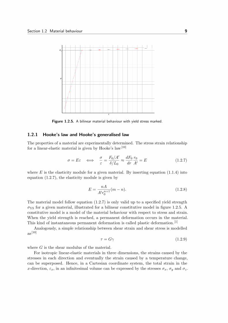
Consider a spring parallel combined with r number of Maxwell models, see figure 2.2.4.Label the parallel added Maxwell models 1, 2, ..., r, the corresponding strains ε1, ε2, ..., εrand stresses σ1, σ2, ..., σr. Let also the strain of the single spring be labelled ε0 andthe stress σ0. Analogously to equation (2.2.4) and equation (2.2.3), the strains for eachMaxwell model and the spring are equal

εi = εj , ∀ i, j ∈ {0, ..., r} (2.2.18)

and the total stress is given by the sum of all partial strains

σ =r∑

k=0

σk. (2.2.19)


ηrη2

k0

k1 k2 kr

η1

Figure 2.2.4. The rheological general Maxwell model. A spring in par-allel with several parallel connected Maxwell models. (Original source –http://upload.wikimedia.org/wikipedia/commons/0/0a/Weichert.svg)

A general differential equation will describe this kind of model and have the form [16](1 +

p∑k=1

akdk

dtk

)σ(t) =

(m+

q∑k=1

bkdk

dtk

)ε(t) (2.2.20)

with q = p or q = p + 1 where p is an integer. The constants m, ak and bk are allnon-negative. As an example, for q = p = 1 having m = E1, b1 = η2

E2(E1 + E2) and

a1 = η2

E2gives the SLS model, equation (2.2.13). The Maxwell model given in equation

(2.2.7) is given with q = p = 1, b1 = η and a1 = ηE . Hence, the springs and dash-pots

are mainly to give a physical representation of the material behaviour. Equation (2.2.20)is sufficient and covers every possible combination of the springs and dash-pots. Forapplication, a predefinition of the differential order has to be made. Further on, thecoefficients ak and bk needs to be fitted to experimental data.

If the sought model is of a higher order differential equation given by equation (2.2.20),it is usually convenient to find the solution with the use of Laplace transformation. [16]

Stress relaxation with the generalised Maxwell model

Simply by applying the constraint given in equation (1.2.32) into equation (2.2.20) givesthe stress relaxation representative differential equation,(

1 +

p∑k=1

akdk

dtk

)σ(t) = mε0 (2.2.21)

where ε0 is the instant deformation. The validity of equation (2.2.21) can be verified bycomparison with the Maxwell model given by equation (2.2.8) and SLS model given byequation (2.2.14).

http://upload.wikimedia.org/wikipedia/commons/0/0a/Weichert.svg


ENon-lineardash-pot

Figure 2.2.5. The rheological Norton model. A spring in parallel with a non-linear dash-pot. (Original source – http://upload.wikimedia.org/wikipedia/commons/d/df/SLS.svg)

2.2.4 Norton model

The Norton creep law follows the behaviour of a non-linear dash-pot, equation (2.2.2).Let a material be described by a linear spring in series with a non-linear dash-pot, seenin figure 2.2.5. Taking the derivative of equation (2.2.6), the total strain rate is given by

dεtot

dt=

1

E

dσ

dt+Bσm. (2.2.22)

Stress relaxation with the Norton model

To model the stress relaxation at constant strain, equation (1.2.32) and equation (2.2.22)yields

1

E

dσ

dt+Bσm = 0 ⇐⇒ dσ

dtσ−m = −BE. (2.2.23)

Integrating both sides with respect to the time t leads to (m 6= 1)

σ−m+1 + C = −BEt(−m+ 1), (2.2.24)

where C is a constant to be found with initial conditions. Assume the initial stress, σ0,at time t = 0 is given by the elastic properties of the material. Hence, it is given thatC = −σ−m+1

0 . Inserting C into equation (2.2.24), an expression of the stress σ over timeis found to be [1]

σ = σ0

(BEt(m− 1)

σ−m+10

+ 1

)− 1m−1

. (2.2.25)

2.2.5 Bolt relaxation based on Norton’s stress relaxation model

Considering equation (2.2.25), equation (1.3.7) and equation (1.3.8), the bolt load canbe expressed as

F (t) = Finitial

(BEt(m− 1)

σ−m+1YS

+ 1

)− 1m−1

, (2.2.26)

where the assumption of the initial first order estimate of the plastic zone size (equation(1.3.9)) fully describing the force relaxation has been made. As no creep data for Avesta308LSi at 288 ◦C was found, material properties and secondary creep for two fictive



Table 2.2.1. Material data and Norton parameters.

Material E [Pa] B m σYS

Fictive material 1 1.2263 · 1011 1.6059 · 10−28 2.234 90.1 · 106

Fictive material 2 1.93 · 1011 5 · 10−48 5 2.1 · 108

material data were used, shown in table 2.2.1. The elasticity module and yield strengthsof Fictive material 1 and Fictive material 2 are typical values for stainless steel at 550 ◦Cand at room temperature, respectively. [18,19] The Norton’s creep parameters B and m forFictive material 1 are somewhat near a real case creep behaviour, but not statisticallysignificant. [19] The Norton parameters for Fictive material 2 are chosen in such a way toyield a larger creep deformation compared to Fictive material 1 during the transient. Thisis to highlight different effects that might occur in materials with large creep deformationscompared to low creep deformations.

Only the Norton model, equation (2.2.22), was modelled with the creep parametersB and m. It is a general version of the Maxwell model (noticed by comparison of §2.2.1and §2.2.4), thus the Maxwell model is discarded. The other creep models presented in§1.2.3 require real data points for curve fitting to yield realistic behaviours. As real datapoints are not available, these are discarded. For example, the general Maxwell modelcould become a more advanced creep model than the Norton model when consisting ofenough number of parameters, although the large number of parameters needed makesit a tedious choice. Also note that the SLS model is the simplest case of the generalMaxwell model. The main difference between the SLS stress relaxation model and theNorton stress relaxation model is the exponential declining versus inverse power functionbehaviour. For long term behaviours it is given that according to the Norton stressrelaxation model the stresses tend to zero, while the SLS stress relaxation model the stresstend to a fix value. By assuming that the material is relaxing until reaching zero stressin elevated temperatures (288 ◦C), the Norton model is the only reasonable candidate formodelling the stress relaxation.

The load relaxation model (equation (2.2.26)), derived from Norton’s stress relaxationmodel, for Fictive material 1 and Fictive material 2 (given in table 2.2.1) can be seen infigure 2.2.6(a) and figure 2.2.6(b). The parameters for fictive material 1 was chosen toproduce a slower relaxation compared to experimental data (table 2.1.1) and, in contrast,the fictive material 2 has a faster relaxation.


0 2 4 6 8 10 12 14 16 18

x 106

0.3

0.4

0.5

0.6

0.7

0.8

0.9

1

t [s]

Load relaxation model for Fictive metal 1

F(t

)/F

initi

al [N

N −

1 ]

Load relaxation model − Fictive metal 1

(a)

0 2 4 6 8 10 12 14 16 18

x 104

0

0.1

0.2

0.3

0.4

0.5

0.6

0.7

0.8

0.9

1

t [s]

Load relaxation for fictive material 2

F(t

)/F

initi

al [N

N−

1 ]

Load relaxation model

(b)

Figure 2.2.6. The load relaxation of (a) Fictive material 1 and (b) Fictive material 2.

I am deathless, I am the eternal LordFor I have spread the seed of the Word.

– Abolqasem Ferdowsi

3

Chapter

Results

This chapter is subdivided into individual sections concerning comparison of the theoreticaland FEM-calculation results.

3.1 Numerical analysis using Ansys

The numerical FEM analysis performed with the software tool called Ansys. The softwarehas tools not only for FEM calculations but also for Computer-aided design (CAD). TheCAD tool is used to create a solid model of the specimen used in the heat transient. Thebolt was also included in the design to simulate the experiment as close to the reality aspossible.

3.1.1 Geometry

The CT-specimen was designed in accordance to the drawing 3003329 Revision 2 shown inappendix A, and the bolt according to 1090900 Revision 03 (drawing given in appendix B).The internal threads and external threads were omitted in the design to reduce calculationtime. Due to the meshing, the threads would yield enormous amount of small elements.The absence of the threads are assumed to not affect the stress in front of the crack tipas the threads are far away from that region. A threaded bolt and CT-specimen can beseen in figure 3.1.1(a) and figure 3.1.1(c), respectively. Their corresponding non threadedgeometries used for the numerical FEM-calculations can be seen in figure 3.1.1(b) for thebolt and figure 3.1.1(d) for the CT-specimen. The assembled bolt and CT-specimen canbe seen in figure 3.1.2.

3.1.2 Input data

Considering the material properties of the bolt and CT-specimen, calculations for fourdifferent cases were performed. The cases are explained below,

1. The entire assembled geometry’s material was assumed to be linear-elastic (followingHooke’s law, §1.2.1) to calculate the stress intensity factor (with Ansys built-incalculation tool for stress intensity factors) and compare it to theoretical results.This was performed to verify the numerical FEM-model and design of the geometry.

34

Section 3.1 Numerical analysis using Ansys 35

(a) (b)

(c) (d)

Figure 3.1.1. The designed solid geometries of (a) the threaded bolt and (b) thecorresponding non threaded bolt, as well as the geometry of (c) the threaded CT-specimen and (d) the corresponding non threaded CT-specimen. The non threadedgeometries were used for numerical FEM-calculations.

2. The material of the bolt is still assumed to be linear-elastic, but the CT-specimenis non-linear following a bilinear stress–strain relationship (the slope of the line atthe plastic region is denoted Eb) and Norton’s creep law. Norton’s creep law is themost common creep law behaviour in the literature. [1,6] The creep law parametersare fictive.

3. Similar to 2 but with other material and creep law parameters corresponding toFictive material 1.

4. Both the bolt and CT-specimen are assumed to follow a bilinear stress-strainrelationship. They are both assumed to follow the material parameters of Fictivematerial 1. Both the bolt and CT-specimen follow Norton’s creep law. The Norton’screep law was chosen to be able verify the theoretical load relaxation (which isbased on the Norton’s creep law) with the numerical FEM-calculation results.

Table 3.1.1 and table 3.1.2 summarise the material and Norton creep parameters for thebolt and CT-specimen in each case. The cases were chosen to show different aspects ofthe impact of the bolt material being prone to creep deformation or not. This is indeeddue to the fact that the bolt have an impact on the remaining bolt tension if being proneto creep behaviours or not. The elasticity module and yield strength differs for highertemperatures and therefore the material parameters for two of the cases are chosen tofollow material parameters for stainless steel at 550 ◦C. Hence the different cases covers

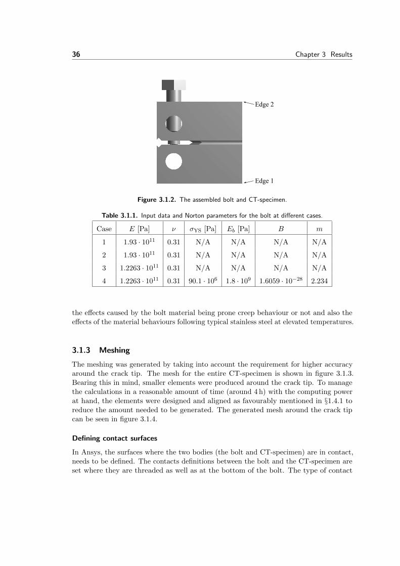
36 Chapter 3 Results

Edge 1

Edge 2

Figure 3.1.2. The assembled bolt and CT-specimen.

Table 3.1.1. Input data and Norton parameters for the bolt at different cases.

Case E [Pa] ν σYS [Pa] Eb [Pa] B m

1 1.93 · 1011 0.31 N/A N/A N/A N/A

2 1.93 · 1011 0.31 N/A N/A N/A N/A

3 1.2263 · 1011 0.31 N/A N/A N/A N/A

4 1.2263 · 1011 0.31 90.1 · 106 1.8 · 109 1.6059 · 10−28 2.234

the effects caused by the bolt material being prone creep behaviour or not and also theeffects of the material behaviours following typical stainless steel at elevated temperatures.

3.1.3 Meshing

The meshing was generated by taking into account the requirement for higher accuracyaround the crack tip. The mesh for the entire CT-specimen is shown in figure 3.1.3.Bearing this in mind, smaller elements were produced around the crack tip. To managethe calculations in a reasonable amount of time (around 4 h) with the computing powerat hand, the elements were designed and aligned as favourably mentioned in §1.4.1 toreduce the amount needed to be generated. The generated mesh around the crack tipcan be seen in figure 3.1.4.

Defining contact surfaces

In Ansys, the surfaces where the two bodies (the bolt and CT-specimen) are in contact,needs to be defined. The contacts definitions between the bolt and the CT-specimen areset where they are threaded as well as at the bottom of the bolt. The type of contact


Table 3.1.2. Input data and Norton parameters for the CT-specimen at different cases.

Case E [Pa] ν σYS [Pa] Eb [Pa] B m

1 1.93 · 1011 0.31 N/A N/A N/A N/A

2 1.93 · 1011 0.31 2.1 · 108 1.8 · 109 5 · 10−48 5

3 1.2263 · 1011 0.31 90.1 · 106 1.8 · 109 1.6059 · 10−28 2.234

4 1.2263 · 1011 0.31 90.1 · 106 1.8 · 109 1.6059 · 10−28 2.234

Figure 3.1.3. Smaller mesh elements in front of the crack tip.

is defined to be bonded as it is assumed the surfaces in contact won’t move relative toeach other during the transient. The contact definition at the bottom of the bolt hasalso a pinball region defined to help Ansys easier detect the contact at that region duringthe transient. This was set due to the entire surface of the bolt end not being in contactwith the CT-specimen in the beginning of the transient.

3.1.4 Bolt pretension

The bolt force was defined with the bolt pretension tool. It was selected at the bottomcylinder of the bolt. The pretension tool could be briefly explained as cutting the cylinderinto two bodies by making the stiffness of the elements along the cut surface to zeroand thereafter pushing then away from each other along shared symmetry axis. Thedeformation is performed until the reaction forces of each of the two bodies reaches a


Figure 3.1.4. The meshed elements in front of the crack tip.

predefined force value. Hence, the bolt pretension tool was set to reach a reaction forceof −16,66 kN where the minus sign denotes the separation of the two bodies. The boltpretension tool does not simulate the real case of screwing the bolt to a certain loadbut is assumed to not have an impact on the results of the stress near the crack tipas it is spatially far away from that region. To make sure the solution converges, fixeddisplacements are also defined. The concerned edges (edge 1 and edge 2) are shown infigure 3.1.2. Edge 1 is fixed in all spatial directions while edge 2 is only constrained alongthe crack front propagation direction.

3.1.5 Ansys results

The stresses along with exaggerated deformation results for case 1 can be seen in figure3.1.5(a) and the true deformation in figure 3.1.5(b). The Stress intensity factor alongthe crack edge is shown in figure 3.1.6 for case 1. It can be noted that it follows thetheoretical results (around 30 MPam1/2 with a 16.66 kN bolt tension). At both ends ofthe crack edge the stress intensity factor is extremely large. This is probably where thethree dimensional effects of the stress distributions makes a difference compared to thecentre of the crack edge. Another reason for the distinction occurring at both ends of thecrack edge could be due to the circular shaped side grooves redistributing the stresses atthe sides of the crack edge differently than in the centre of the crack edge.

The stress and deformation results for case 2 at the end of the bolt pretension andafter the heat transient can be seen in figure 3.1.7. Zoomed results of the crack tip shapeare also included. As can be noticed in the zoomed in crack tips, during the transientthe crack tip is blunting. Additionally, the stress relaxation effect is clearly shown.

The results for case 3 and case 4 are seen in figure 3.1.8 and figure 3.1.9, respectively,but without any crack tip blunting occurrence. Almost no stress relaxation could beobserved.


(a)

(b)

Figure 3.1.5. The stresses and (a) exaggerated deformations as well as (b) the truedeformation of the CT-specimen. Results carried with the use of Ansys on material dataof case 1.


0 0.002 0.004 0.006 0.008 0.01 0.012 0.014 0.016 0.018 0.022.8

3

3.2

3.4

3.6

3.8

4

4.2

4.4

4.6

4.8x 10

7

Crack edge position [m]

Str

ess

inte

nsity

fact

or [P

a m

1/2 ]

Stress intensity along crack edge

Stress intensity factor

Figure 3.1.6. Stress intensity factor along the crack edge for case 1.


(a) (b)

(c) (d)

Figure 3.1.7. The stress and deformation with case 2 parameters for (a) the initialstate of the CT-specimen and (b) a zoomed picture of the crack tip. The correspondingresults at the end of the transient for (c) the CT-specimen and (d) the zoomed in cracktip.


(a) (b)

(c) (d)

Figure 3.1.8. The stress and deformation with case 3 parameters for (a) the initialstate of the CT-specimen and (b) a zoomed picture of the crack tip. The correspondingresults at the end of the transient for (c) the CT-specimen and (d) the zoomed in cracktip.

(a) (b)

Figure 3.1.9. The stress and deformation with case 4 parameters for (a) the initialstate of the CT-specimen and (b) at the end of the transient for the CT-specimen.

Section 3.2 Comparison of theoretical models to numerical FEM calculation results 43

3.2 Comparison of theoretical models to numerical FEM calcu-lation results

The remaining bolt load of the numerical FEM-calculation results together with thetheoretical bolt load relaxation model for case 3 and case 4 are shown in figure 3.2.1.The bolt load relaxation model and the Ansys bolt load results during the transient forcase 2 is given by figure 3.2.2. For case 2, the rate of change of the bolt load from theFEM-calculation results compared to the relaxation model are almost equal at the end ofthe transient.


0 2 4 6 8 10 12 14 16 18

x 104

0.97

0.975

0.98

0.985

0.99

0.995

1

t [s]

Load relaxation. E=1.2263e11 [Pa], σYS

=90.1e6 [Pa], B=1.6059e−28, m=2.234

F(t

)/F

initi

al [N

N −

1 ]

Relaxation modelAnsys − CT−specimennon−linear

Ansys − Bolt + CT−specimennon−linear

Figure 3.2.1. Theoretical bolt load relaxation model (with CT-specimen parameters forcase 3 and case 4) and the Ansys case 3 and case 4 results.

0 2 4 6 8 10 12 14 16 18

x 104

0

0.1

0.2

0.3

0.4

0.5

0.6

0.7

0.8

0.9

1

t [s]

Load relaxation for fictive material 2

F(t

)/F

initi

al [N

N−

1 ]

Load relaxation modelAnsys − CT−specimennon−linear

Figure 3.2.2. Theoretical bolt load relaxation model (with CT-specimen parameters forcase 2) and the Ansys case 2 results.

4

Chapter

Conclusions

With Norton’s creep model, it has been shown that the bolt tension can be fairly wellestimated during the transient compared to the numerical FEM-calculation performed.Although, this is of no worth if the experimental results won’t show a similar behaviour.Hence for verification, further experiments are required, see §4.3.

The relaxation model could be calibrated if needed to fit the numerical FEM-calculation results. Preferably by increasing or decreasing σYS by a factor to minimisethe error for a particular load and material case.

The long term effects of the numerical FEM-calculated (and experimental) bolt loadrelaxation rate is well described by the relaxation model.

One concern of the model and numerical FEM-calculations are the assumptions ofconstant temperature. During the heat transient (elevation of the temperature from roomtemperature to 288 ◦C) the material expands. The expansion of the material might affectthe initial stresses, that is, increasing or decreasing the magnitude of the forces whilehave reached the desired temperature. The expansion effect on the initial stresses wasdiscarded as it could be assumed that larger or smaller bolt loads were initially appliedto the specimen. The shape of the bolt load relaxation curves would still be similar tothe achieved results. The expansion effect changes the geometrical values of the specimen(effecting the theoretical value of the stress intensity factor). The geometrical changes ofthe specimen were also discarded, assuming the changes were negligible.

4.1 Remarks about the theoretical results

The theoretical bolt load relaxation model is derived by linear elastic material assumptions.The stresses being proportional to the stress intensity factor is only valid far away fromthe crack tip. If large creep rates are present, the assumptions made during the derivationof the bolt load relaxation could result in an inaccurate model. The stress intensityfactor for a CT-specimen assumes sharp crack tips and does not take the crack bluntinginto account. Although, due to the stresses decreasing with an increased radius ofcrack tip curvature, for conservative safety verifications this is not to be of any concern.This is explained by the linear elastic case brings a harsher crack tip state than theductile/plastic/non-linear case.

45

46 Chapter 4 Conclusions

It can be noted that neither the Fictive material 1 nor Fictive material 2 has similardecreases in bolt load relaxation as to the experimental results carried on by KTH, mostprobably due to the creep parameters not corresponding to the material used.

An additional assumption that could be questioned, due to the lack of verificationwith experimental results, is the models eligibility due to the first order estimation of theinitial plastic zone size. It is not verified if that is the best position in front of the cracktip where the stress is explaining the relaxation.

No reversible creep effects has been taken into account after the transient.For all assumptions to be verified and eligible, additional experiments are required.

4.2 Remarks about the numerical FEM-calculation results

The performed numerical FEM-calculation results of the linear elastic case are coherentwith the theory. The stress intensity factor yield similar results to the theory, thus themodel in Ansys are likely to be correct. The crack tip is simply sharp enough for thematerial used after the load being applied. Even though the results in this matter seemssatisfactory, they have to be verified for each material used.

The material and settings according to case 2 show a large plasticity in front of thecrack tip. The stresses in the plastic zone decrease as the material relaxes as expected.Interestingly, the crack tip starts to blunt during the relaxation. Thus, the strain is notconstant. The blunting is affecting the stresses in front of the crack tip in such a waythat an increase in the crack tip curvature radius decreases the stresses further alongwith the decrease of stresses only due to the stress relaxation. If a conservative model isto be used for modelling the stresses in front of the crack tip, the blunting is not of anyconcern.

In case 3 (and case 4), no crack tip blunting could be observed. This is most likelydue to the low creep rates for that particular case.

4.3 Future work

The lack of experimental creep results for different stresses at different temperaturesfor Avesta 308LSi brought the biggest challenges to this report. Therefore, an uni-axialstress relaxation or creep deformation experiment is highly recommended for all materialsused in the interested temperature regime. This also applies for the bolt material. Theresults of such experiment could be used to curve fit the various creep models presentedin this report. Further on, the use these creep models in the numerical FEM analysis toverify the validity in the three dimensional case for the CT-specimen should thereby bedone. By verifying the numerical FEM-calculation results with the already performedexperimental bolt relaxation results, the material creep behaviour in the CT-specimencould be assumed to be completely described.

For further validity, it is largely recommended to measure the bolt load with certaintime intervals during the experimental transient compared to only the initial and remainingbolt load after the experimental transient. Perhaps the measurements could be made at

Section 4.3 Future work 47

every 5h (to extract additional 9 data points during the 50h transient) to enable thepossibility to verify the shape of the bolt relaxation model.

To not have to concern about the bolt material relaxing and thereby affecting theexperimental results, choose the bolt material with care that have significantly lowercreep rates than the weld material inside the CT-specimen at the temperatures of thetransient/heat treatment cycle.

Verification and comparison of the analytical bolt load relaxation model derived fromthe Norton model with the other models presented could be beneficial.

Bibliography

[1] Anderson TL. Fracture Mechanics – Fundamentals and Applications. 2nd ed. BocaRaton (FL): CRC Press; 1994.

[2] ASTM Standard E647-13a. Standard Test Method for Measurement of FatigueCrack Growth Rates. West Conshohocken (PA): ASTM International; 2013.DOI: 10.1520/E0647.

[3] ASTM Standard E1820-13. Standard Test Method for Measurement ofFracture Toughness. West Conshohocken (PA): ASTM International; 2013.DOI: 10.1520/E1820.

[4] Carlsson J. Brottmekanik. Stockholm (Sweden): Ingenjorsforlaget; 1976. Swedish.

[5] Nilsson F. Fracture Mechanics – from Theory to Application. Stockholm (Sweden):Department of Solid Mechanics, KTH; 2001.

[6] Dowling NE. Mechanical Behavior of Materials. 4th ed. Harlow (United Kingdom):Pearson Education; 2012.

[7] Jenssen A, Engman U. Lastrelaxation i bultbelastade CT- och WOL-prov – Sam-manstallning av erfarenheter fran genomforda provningar. Nykoping (Sweden):Studsvik Nuclear AB; 2010. Studsvik/N-10/142. Swedish.

[8] Kittel C. Introduction to Solid State Physics. 8th ed. Hoboken (NJ): John Wiley &Sons; 2004.

[9] Robinett RW. Quantum Mechanics – Classical Results, Modern Systems, andVisualized Examples. 2nd ed. Oxford (NY): Oxford University Press; 2006.

[10] Lundh H. Grundlaggande hallfasthetslara. Stockholm (Sweden): Department ofSolid Mechanics, KTH; 1994. Swedish.

[11] Lapidus L, Pinder GF. Numerical Solution of Partial Differential Equations inScience and Engineering. New York: John Wiley and Sons; 1982.

48

Bibliography 49

[12] Zienkiewics OC, Taylor RL. The Finite Element Method. 4th ed. New York:McGraw-Hill; 1989.

[13] Rizzo FJ. An Integral Equation Approach to Boundary Value Problems of ClasscalElastostatics. Quarterly of Applied Mathematics. 1967;25:83–95.

[14] Finch RF. Performance welding. Osceola (WI): MBI; 1997.

[15] Anttonen JP, Astrom B. Tillverkning av testblock for CT-provstavar. Stockholm(Sweden): Swerea KIMAB; 2011. Report no. 658010. Swedish.

[16] Mainardi F, Spada G. Creep, Relaxation and Viscosity Properties for Basic FractionalModels in Rheology. The European Physical Journal, Special Topics. 2011;193:133–160.

[17] Rade L, Westergren B. Mathematics Handbook for Science and Engineering. 5th ed.Lund (Sweden): Studentlitteratur; 2004.

[18] ASM Aerospace Specification Metals, Inc [homepage on the Internet]. PompanoBeach (FL): ASM Aerospace Specification Metals, Inc; [cited 2014 Mar 27]. AISIType 304L Stainless Steel. Available from: http://asm.matweb.com/search/

SpecificMaterial.asp?bassnum=MQ304L.

[19] Hayhurst DR, Vakili-Tahami F, Zhou JQ. Constitutive equations for time indepen-dent plasticity and creep of 316 stainless steel at 550 ◦C. The International Journalof Pressure Vessels and Piping . 2003 Feb;80(2):97–109.

http://asm.matweb.com/search/SpecificMaterial.asp?bassnum=MQ304L

http://asm.matweb.com/search/SpecificMaterial.asp?bassnum=MQ304L

Appendices

51

A

Appendix

Drawing 3003329 Revision 2

CLASSIFIED

53

B

Appendix

Drawing 1090900 Revision 03

CLASSIFIED

55

Modelling Stress Relaxation in Bolt Loaded...

Documents

Transcript of Modelling Stress Relaxation in Bolt Loaded...