Modelling start-up injection of CO2 into highly-depleted gas fields

Andrea Sacconi and Haroun Mahgerefteh*

Department of Chemical Engineering, University College London, London WC1E 7JE, UK

Abstract The development and verification of a homogeneous relaxation model for simulating the highly transient flow

phenomena taking place during the start-up injection of CO2 into deep highly depleted gas fields is presented. The

constituent mass, momentum, and energy conservation equations, incorporating a relaxation time to account for non-

equilibrium effects, are solved numerically for single and two-phase flows along the steel lined injection well leading

to the storage reservoir. Wall friction, gravitational field effects and heat transfer between the expanding fluid and the

outer well layers are taken into account as source terms in the conservation equations. At the well inlet, the opening of

the upstream flow regulator valve is modelled as an isenthalpic expansion process; whilst at the well outlet, a

formation-specific pressure-mass flow rate correlation is adopted to characterise the storage site injectivity. The

testing of the model is based on its application to CO2 injection into the depleted Golden Eye Reservoir in the North

Sea for which the required design and operational data are publically available. Three injection scenarios involving a

rapid, medium and slow linear ramping up of the injected CO2 flow rate to the peak nominal value of 33.5 kg/s are

simulated. In each case, the predicted pressure and temperature transients at the top and bottom of the well are

employed to ascertain the risks of well-bore thermal shocking, and interstitial ice or CO2 hydrate formation leading to

its blockage due to the rapid expansion cooling of the CO2. The results demonstrate the efficacy of the proposed

model as a tool for the development of optimal injection strategies and best-practice guidelines for the minimisation of

the risks associated with the start-up injection of CO2 into depleted gas fields.

Keywords: Global warming, Carbon Capture and Storage, CO2 injection, Transient flow modelling

*corresponding author h.mahgerefteh@ucl.ac.uk

1. Introduction

According to the IEA Energy Technology Perspective [1], Carbon Capture and Sequestration (CCS) is expected to

play a key role in moving the CO2 emitting energy intensive industries, such as iron and steel, cement and oil

refineries onto a pathway consistent with limiting the increase in global average temperatures to well below 2°C above

pre-industrial levels as agreed at the Paris Climate Conference in 2015. The safe and cost effective storage of the

enormous amounts of CO2 captured from these sources is an essential element of CCS and therefore of fundamental

importance in ensuring its success. Highly-depleted gas fields offer excellent potential for the permanent storage of

the captured CO2 [2]. In the case of the UK for example, the Southern North Sea and the East Irish Sea depleted gas

reservoirs provide almost 95% of the storage capacity required to meet UK’s CO2 reduction commitments for the

period 2020-2050 [3].

As compared to saline aquifers, depleted gas fields are better characterized given the availability of geological data,

such as pressure, porosity and permeability, derived from years of gas production. They have seals that have

successfully retained hydrocarbon gas for millions of years, and may offer a shorter route to practical implementation

for early Carbon Capture and Storage (CCS) projects [4].

The UK has completed three large FEED study projects for offshore CO2 storage at Hewett, Golden Eye and

Endurance sites [5]. However, CO2 storage at full industrial scale has only been demonstrated at a small number of

sites around the world: Sleipner, In Salah & Snøvit [6], Ordos [7], and the Quest project [8].

In order to boost the confidence of both investors and the public and thus facilitate the full-scale deployment of CCS,

it is of paramount importance to guarantee that the storage site will be of high quality and operate in a safe manner.

However, given the low reservoir pressures along with the unique thermodynamic properties of CO2, the start-up

injection of CO2 into depleted low-pressure gas fields presents significant safety and operational challenges.

The most practical cost-effective option for transporting the captured CO2 involves the use of sub-sea pipelines with

the CO2 in the dense or liquid phase, i.e. above 75 bar given the lower pressure drop along the pipeline as compared to

the gas phase and the larger line pack [9–12]. As the sea temperature will be well below the CO2 critical temperature

(31.1 oC), the fluid will arrive in the liquid state. Given the much lower wellhead pressure, the uncontrolled injection

of the CO2 into the wellhead will lead to its rapid quasi adiabatic expansion (often referred to as Joule Thomson

cooling) into a two-phase mixture leading to temperatures well below zero oC [13].

In practice, the rapid expansion cooling could pose several operational and safety risks, namely:

CO2 hydrate and ice formation following contact of the cold CO2 with the interstitial water around the

wellbore and the formation water in the perforations at the near well zone. The former poses the risk of well

blockage, while the latter may severely reduce the reservoir injectivity and ultimately its storage capacity;

thermal stress shocking of the wellbore casing steel leading to its fracture and the escape of CO2;

thermal stress shocking of the reservoir rocks leading to fracture thus changing the reservoir permeability and

reducing ‘its CO2 locking’ effectiveness;

superheating of the liquid CO2 at the wellhead leading to its violent evaporation and over-pressurisation

followed by CO2 backflow into the injection system.

As such, developing appropriate start-up injection strategies where the rate of injection of CO2 is gradually increased

in a controlled manner is of paramount importance for avoiding the above risks. Key to this is the availability of

reliable mathematical models for predicting the behaviour of the injected CO2, in particular its variation of pressure

and temperature along the well and ultimately at the point of entry into the depleted reservoir. The alternative is the

heating of the CO2 stream prior to injection, which is highly costly given the significant volumes involved.

Driven by the push to reduce CO2 emissions along with the economic incentives associated with enhanced natural gas

recovery involving CO2 injection into depleted natural gas reservoirs, several, almost exclusively modelling studies

focusing on the associated temperature and pressure transients with various degrees of sophistication have been

reported in the open literature. The following is a critical review of the main models. The review does not cover the

much simpler case of injection of CO2 into aquifers [14]. Given the much higher aquifer pressures, the rapid fluid

expansion transient phenomenon associated with the injection of CO2 in depleted gas fields are not expected here and

hence irrelevant to the scope of the present work.

Olenbuurg [15] employed the commercially available ToughTOUGH2 module to simulate the radial variation of the

reservoir temperature at the bottom of the well for different natural gas reservoir permeabilities and constant injection

CO2 flow rates, reporting a cooling of approximately 20 °C. Goodarzi et al [16] employed a coupled flow,

aeromechanical and heat transfer model for the injection and sequestration of CO2 in Ohio Valley. However their

model was limited to simulating the impact on the injection zone and the surrounding formations in order to evaluate

the risk of induced fracturing of the storage formation following exposure to the incoming low temperature CO2

stream.

Linga and Lund [17] developed a sophisticated two-fluid model applied to CO2 injection wells incorporating the

Span–Wagner equation-of-state [18]. However, much the same as Li et al [19], the application of their model was

limited to predicting the resulting temperature and pressure profiles following well blowout and during shut in.

Temperatures as low as − 48◦C were predicted upon blowout concluding that this temperature was not necessarily low

enough to cause damage to the steel pipe itself, but likely to pose a hazard due to mechanical stresses that arise due to

thermal contraction.

Lu and Connell [20] presented a model to simulate the flow of CO2 and its mixtures in non-isothermal wells.

However their model was based on steady state flow, therefore incapable of dealing with the rapid transients occurring

during the start-up injection phase. Paterson et al [21] too developed a steady state flow model in order to predict the

bottom hole well pressure following the injection of CO2 for Enhanced Oil Recovery (EOR).

Lindeberg et al [22] used the Bernoulli’s pressure drop equation along with heat transfer and frictional effects to

predict injection well temperature profile for the steady state injection of CO2 for Sleipner CO2 storage project to

show that adiabatic conditions flow conditions along the well could be assumed after a few months even if the

injection is regularly stopped for one to two weeks for servicing. Pan et al [23] using the drift flux conceptual model

presented analytical solutions for compressible two-phase flow thorough a 1000 m , 0.1m dia. well bore under

isothermal and homogenous equilibrium flow conditions accounting for phase slip. Verifying their predictions of the

gas phase velocity and drift velocity versus well depth against the results of the commercially numerical wellbore flow

simulator T2Well, the authors used their model to evaluate how the bottom hole pressure in a well in which CO2 is

leaking upward responds to the mass flow rate of CO2–water mixture. Lu and Connell [24] presented a transient flow

model based on the homogenous equilibrium where the constituent phases are assumed to be at thermal and

mechanical equilibrium coupled with a steady state heat transfer model for the injection of liquid CO2 into a 560 m

deep 0.03m dia. well for a field trial of CO2 enhanced coal bed methane recovery. Critically important information

such as the CO2 injection rate and its variation with time was not given. The subsequent fluid bottom-hole pressure

and temperature data for a period of 3.5 h following the completion of the injection process were simulated. The

model was incapable of handling the injection start-up process were the transient variations in the CO2 temperature

and pressure are expected to be most pronounced. Relatively poor agreement between model predictions of the

transient temperature data against the recorded data were reported despite significant modifications of the heat transfer

model.

Munkejord et al [25] conducted three case studies relating to the transport and injection of CO2. In the first case

study, the authors generated the pressure/enthalpy phase diagram for compression/cooling trajectories for pure

CO2 and 5% CH4 / 95% methane in order to determine the fluid phase arriving at the well head. The second case

study dealt with the abandoned Vattenfall CCS demonstration project involving the retrofitting of a post-combustion

capture unit to the Nordjyllandsværket coal-fired power plant and transporting the captured CO2 to an onshore

saline aquifer using a 24 km pipeline. The commercial software ,OLGA incorporating a drift flux model by Kjell and

Bendiksen [26] was employed to track the well bottom hole pressure/time response following a variable mass flow

rate injection loading. Given that CO2 is injected into a high pressure (213 bar) aquifer, the relatively slow mass flow

ramping rate employed, along with CO2 remaining in the dense phase throughout the injection well, as expected,

given the relatively large velocity of sound in the fluid (ca. 1000 m/s), the bottom hole pressure reacted almost

instantaneously in response to a change in the feed mass flow rate. In case study 3, the OLGA was employed to

simulate the pressure and temperature/time profiles for the depressurisation of a subsea pipeline transporting

captured CO2 from flue gas emitted by the combined heat and power plant at Mongstad into suitable locations on

the Norwegian Continental Shelf.

Li et al [27] coupled a steady-state thermo-hydraulic model describing flow of CO2 in an injection well with a

transient model for radial heat conduction in the rock formation surrounding the well. The model enabled the analysis

of slow transients in the flow and heat transfer occurring during the temperature equilibration between the well and the

formation upon a steady-state injection conditions. The model was validated against real data, showing a good

agreement with the bottom hole pressure and temperature measured in a test involving injection of supercritical CO2.

However, due to the underlying assumption of steady-state flow, the model is not suitable for analysis of start-up

injection where large temperature variations in the well fluid are induced as a `consequence of the rapid expansion of

the CO2 in the wellhead.

Lund et al [28] employed a heat conduction model based on finite volume method for determining the heat transfer

from the well to the casing, annular seal, and rock formation following the injection of CO2 for EoR applications.

Their predictions of the temperature variations at various locations in and around a given well during CO2 injection

were found to be in relatively good agreement with those based on small scale laboratory experiments. The authors

used their model to conclude, as expected, that by replacing cement with an annular sealant material with higher

thermal conductivity, the temperature difference across the seal can be significantly reduced thus reducing the risk

associated with the thermal shocking of the well.

In a report by Shell [29] (see Section 4), the transient variations of the well head and well bottom pressure and

temperature were reported for the injection of CO2 into the depleted Golden Eye reservoir using OLGA. However no

information is publically available describing the detailed development of the above flow model in pipes for the

simulation of the more complex start-up injection of CO2 through a vertical well discharging into the reservoir at

different ramping up injection rates.

Based on the above review, it is clear that much of the reported models on CO2 injection into well bores are based on

steady-state flow assumption where the rapid pressure and temperature transients associated with the start-up injection

process cannot be handled. The drift-flux flow models dealing with multi-phase flow behaviour usually contain

several empirical parameters that must be determined experimentally. They are also notoriously prone to numerical

stabilities or singularities at either flow regime transitions or when the liquid volume fraction approaches zero [30].

The use of the sophisticated commercial simulator OLGA, also incorporating drift-flux flow complicates the model

validation since little information is publically available regarding its details.

In this paper the development and verification of a mathematical model for simulating the transient flow phenomena

taking place during the start-up injection of CO2 into highly depleted gas fields is presented. The formulation is based

on a Homogeneous Relaxation Model (HRM), where mass, momentum, and energy conservation equations are

considered for single or two-phase flows. The model accounts for phase and flow dependent fluid/wall friction and

heat transfer, variable well cross sectional area as well as deviation of the well from the vertical.

At the well inlet, the opening of the upstream flow regulator valve is modelled as an isenthalpic expansion process;

whilst at the well outlet, a pre-defined site-characteristic pressure-mass flow rate correlation is used to simulate the

migration of the CO2 into the geological substrate. The developed model is next employed to perform a detailed

sensitivity analysis of the most important parameters affecting the CO2 flow behaviour, including the upstream

temperature, pressure and time variant mass flow rate; the latter being representative of the feed pressure ramping up

process. These investigations are intended to demonstrate the efficacy of the injection model presented as a practical

tool for the development of optimal injection strategies and best-practice guidelines for minimising the risks

associated with the start-up injection of CO2 into depleted gas fields.

2. Model formulation

2.1 Wells and injection scenarios

Wells are an essential component of any CO2 storage project. They are the only way by which CO2 can be discharged

into underground reservoirs in the timeframes required. It is important to recognise that the injected CO2 is not stored

in the wells. The well represents the transportation route through which the CO2 will be released into reservoirs and

then remain safely trapped. Wells are drilled for a range of purposes such as exploration, appraisal, production,

injection or monitoring. Well objectives strongly influence its design, depth, size and cost. The information gathered

from existing wells drilled and used by oil and gas operators proves to be very useful in characterising the subsurface

geology of a site [5]. A schematic of typical well for the injection of CO2 into a depleted gas field is represented in

Figure 1. The well is composed of various layers and surrounded by a formation, whose composition varies from site

to site. Wells have to be carefully analysed in order to assess their suitability for CO2 injection in depleted oil and gas

fields [31].

Before the steady injection of CO2 into the reservoir can be started, it is necessary to perform time-dependent

operations to estimate important reservoir properties, e.g. permeability and pressure. Such operations include start-up,

shut-in and emergency shut-down, which prove to be critical in the overall design of the well [9]. Even after steady

injection conditions are reached, the well may be shut in and started up for maintenance of the upstream transportation

system or other routine checks. It is therefore of paramount importance to be able to predict the behaviour of the CO2,

in terms of pressure and temperature, particularly at the top and bottom of the well in order to identify and quantify

potential risks.

2.2 Fluid dynamics

The following gives an account of the extension of our previously developed Homogeneous Relaxation Model

((HRM) [32,33]) employed for the simulation of the time-dependent flow of CO2 injected into the well. The system of

four partial differential equations for the CO2 liquid/gas mixture, to be solved in the well tubing can be written in the

well-known conservative form as follows:

Figure 1: Schematic representation of a deep well CO2 injection and storage facility

𝜕

𝜕𝑡𝑼 +

𝜕

𝜕𝑧𝑭(𝑼) = 𝑺𝟏 + 𝑺𝟐 (1)

Where, we define;

𝑼 = (

𝜌𝐴𝜌𝑢𝐴𝜌𝐸𝐴𝐴

) , 𝑭(𝑼) = (

𝜌𝑢𝐴

𝜌𝑢2𝐴 + 𝐴𝑃𝜌𝑢𝐻𝐴0

), 𝑺𝟏 =

(

0

𝑃𝜕𝐴

𝜕𝑧00 )

, 𝑺𝟐 = (

0𝐴(𝐹 + 𝜌𝛽𝑔)

𝐴(𝐹𝑢 + 𝜌𝑢𝛽𝑔 + 𝑄)0

) (2)

In the above, the first three equations correspond to mass, momentum, and energy conservation respectively. The

fourth equation accounts for the fact that the well bore cross-sectional area 𝐴 at any location along the well does not

change with time, but may vary along the well. 𝑢 and 𝜌 are the mixture velocity and density respectively. 𝑃 is the

mixture pressure, while 𝐸 and 𝐻 represent the specific total energy and total enthalpy of the fluid, respectively. These

are in turn are defined as:

𝐸 = 𝑒 + 1

2 𝑢2 (3)

𝐻 = 𝐸 + 𝑃

𝜌 (4)

where, 𝑒 is the specific internal energy. 𝑧 denotes the axial coordinate, 𝑡 the time, 𝐹 the viscous friction force, 𝑄 the

heat flux, and 𝑔 the gravitational acceleration. Given the rapid transients during decompression, phase slip is ignored.

However, non-equilibrium liquid-vapour transition is accounted for by a relaxation to thermodynamic equilibrium

through the following equation [34]:

𝜕𝑥

𝜕𝑡+ 𝑢

𝜕𝑥

𝜕𝑧= 𝑥𝑒 − 𝑥

𝜃 (5)

where, 𝑥 is the mixture vapour quality and 𝜃 is a relaxation time accounting for the delay in the phase change

transition. The mixture density 𝜌 is defined as:

1

𝜌=

𝑥

𝜌𝑠𝑣(𝑃)+

1 − 𝑥

𝜌𝑚𝑙(𝑃, 𝑒𝑚𝑙) (6)

while the mixture internal energy is defined as:

𝑒 = 𝑥𝑒𝑠𝑣(𝑃) + (1 − 𝑥)𝑒𝑚𝑙 (7)

Where, the subscripts 𝑠𝑣 and 𝑚𝑙 refer to the saturated vapour and meta-sTable (super-heated) liquid phases

respectively.

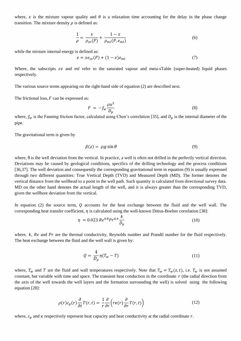
The various source terms appearing on the right-hand side of equation (2) are described next.

The frictional loss, 𝐹 can be expressed as:

𝐹 = −𝑓𝑤𝜌𝑢2

𝐷𝑝 (8)

where, 𝑓𝑤 is the Fanning friction factor, calculated using Chen’s correlation [35], and 𝐷𝑝 is the internal diameter of the

pipe.

The gravitational term is given by

𝛽(𝑧) = 𝜌𝑔 sin𝜃 (9)

where, θ is the well deviation from the vertical. In practice, a well is often not drilled in the perfectly vertical direction.

Deviations may be caused by geological conditions, specifics of the drilling technology and the process conditions

[36,37]. The well deviation and consequently the corresponding gravitational term in equation (9) is usually expressed

through two different quantities: True Vertical Depth (TVD) and Measured Depth (MD). The former denotes the

vertical distance from the wellhead to a point in the well path. Such quantity is calculated from directional survey data.

MD on the other hand denotes the actual length of the well, and it is always greater than the corresponding TVD,

given the wellbore deviation from the vertical.

In equation (2) the source term, 𝑄 accounts for the heat exchange between the fluid and the well wall. The

corresponding heat transfer coefficient, 𝜂 is calculated using the well-known Dittus-Boelter correlation [38]:

𝜂 = 0.023 𝑅𝑒0.8𝑃𝑟0.4𝑘

𝐷𝑝 (10)

where, 𝑘, 𝑅𝑒 and 𝑃𝑟 are the thermal conductivity, Reynolds number and Prandtl number for the fluid respectively.

The heat exchange between the fluid and the well wall is given by:

𝑄 = 4

𝐷𝑝𝜂(𝑇𝑤 − 𝑇) (11)

where, 𝑇𝑤 and 𝑇 are the fluid and wall temperatures respectively. Note that 𝑇𝑤 = 𝑇𝑤(𝑧, 𝑡), i.e. 𝑇𝑤 is not assumed

constant, but variable with time and space. The transient heat conduction in the coordinate 𝑟 (the radial direction from

the axis of the well towards the well layers and the formation surrounding the well) is solved using the following

equation [28]:

𝜌(𝑟)𝑐𝑝(𝑟)𝜕

𝜕𝑡𝑇(𝑟, 𝑡) =

1

𝑟

𝜕

𝜕𝑟(𝑟𝜅(𝑟)

𝜕

𝜕𝑟𝑇(𝑟, 𝑡)) (12)

where, 𝑐𝑝 and 𝜅 respectively represent heat capacity and heat conductivity at the radial coordinate 𝑟.

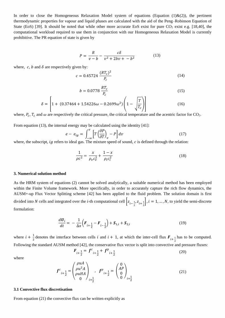
In order to close the Homogeneous Relaxation Model system of equations (Equation (1)&(2)), the pertinent

thermodynamic properties for vapour and liquid phases are calculated with the aid of the Peng–Robinson Equation of

State (EoS) [39]. It should be noted that while other more accurate EoS exist for pure CO2 exist e.g. [18,40], the

computational workload required to use them in conjunction with our Homogeneous Relaxation Model is currently

prohibitive. The PR equation of state is given by

𝑃 = 𝑅

𝑣 − 𝑏−

𝑐𝛿

𝑣2 + 2𝑏𝑣 + − 𝑏2 (13)

where, 𝑐, 𝑏 and 𝛿 are respectively given by:

𝑐 = 0.45724 (𝑅𝑇𝑐)

2

𝑃𝑐 (14)

𝑏 = 0.0778 𝑅𝑇𝑐𝑃𝑐

(15)

𝛿 = [1 + (0.37464 + 1.54226𝜔 − 0.2699𝜔2)(1 − √𝑇

𝑇𝑐)] (16)

where, 𝑃𝑐, 𝑇𝑐 and 𝜔 are respectively the critical pressure, the critical temperature and the acentric factor for CO2.

From equation (13), the internal energy may be calculated using the identity [41]:

𝑒 − 𝑒𝑖𝑔 = ∫ [𝑇 (𝜕𝑃

𝜕𝑇)𝑣− 𝑃]𝑑𝑣

𝑣

−∞

(17)

where, the subscript, 𝑖𝑔 refers to ideal gas. The mixture speed of sound, 𝑐 is defined through the relation:

1

𝜌𝑐2=

𝑥

𝜌𝑣𝑐𝑣2 +

1 − 𝑥

𝜌𝑙𝑐𝑙2 (18)

3. Numerical solution method

As the HRM system of equations (2) cannot be solved analytically, a suitable numerical method has been employed

within the Finite Volume framework. More specifically, in order to accurately capture the rich flow dynamics, the

AUSM+-up Flux Vector Splitting scheme [42] has been applied to the fluid problem. The solution domain is first

divided into 𝑁 cells and integrated over the 𝑖-th computational cell [𝑧𝑖−

1

2

, 𝑧𝑖+

1

2

] , 𝑖 = 1,… ,𝑁, to yield the semi-discrete

formulation:

𝑑𝑼𝑖𝑑𝑡

= − 1

Δ𝑥(𝑭

𝑖+ 12− 𝑭

𝑖− 12) + 𝑺1,𝑖 + 𝑺2,𝑖 (19)

where 𝑖 + 1

2 denotes the interface between cells 𝑖 and 𝑖 + 1, at which the inter-cell flux 𝑭

𝑖+ 1

2

has to be computed.

Following the standard AUSM method [42], the conservative flux vector is split into convective and pressure fluxes:

𝑭𝑖+ 12= 𝒇𝑐

𝑖+ 12+ 𝒇𝑝

𝑖+ 12 (20)

where

𝒇𝑐𝑖+ 12= (

𝜌𝑢𝐴

𝜌𝑢2𝐴𝜌𝑢𝐻𝐴0

)

𝑖+12

, 𝒇𝑝𝑖+ 12= (

0𝐴𝑃00

)

𝑖+12

(21)

3.1 Convective flux discretisation

From equation (21) the convective flux can be written explicitly as

𝒇𝑐 = �̇�(

1𝑢𝐻0

) = �̇�𝚿 (22)

where, �̇� is the area-weighted mass flux:

�̇� = 𝜌𝑢𝐴 (23)

The numerical flux at cell interface 𝑖 + 1

2 is then defined as:

𝒇𝑐𝑖+ 12= �̇�∗𝚿∗ = �̇�∗

1

2(𝚿𝑖 + 𝚿𝑖+1) +

1

2|�̇�∗|(𝚿𝑖 − 𝚿𝑖+1) (24)

In order to express �̇�, the interface speed of sound 𝑎𝑖+

1

2

and the left and right Mach numbers are defined as follows:

𝑎𝑖+ 12= 𝑎𝑖 + 𝑎𝑖+1

2, 𝑀𝑖 =

𝑢𝑖𝑎𝑖+ 12

, 𝑀𝑖+1 = 𝑢𝑖+1𝑎𝑖+ 12

(25)

The interface Mach number is next defined as:

�̃�𝑖+ 12= ℳ4

+(𝑀𝑖) + ℳ4−(𝑀𝑖+1) (26)

where ℳ+ and ℳ− are the polynomials introduced by Liou [40] and the subscripts indicating the order of the

polynomial used:

ℳ1± =

1

2(𝑀 ± |𝑀|) (27)

ℳ2± = ±

1

4(𝑀 ± 1)2 (28)

ℳ4± = {

ℳ1±

𝑀, where |𝑀| ≥ 1

± ℳ1±(1 ∓ 16𝐵ℳ2

∓)

(29)

with 𝐵 =1

8.

In order to approximate numerically the area-weighted mass flux introduced in equation (23), we define:

�̇�∗ = 𝑎𝑖+ 12[(𝜌𝐴)𝑖2

(𝑀𝑖+12+ |𝑀

𝑖+12|) +

(𝜌𝐴)𝑖+12

(𝑀𝑖+12− |𝑀

𝑖+12|)] (30)

where, 𝑀𝑖+1

2

= �̃�𝑖+

1

2

. However, at low Mach numbers this approximation approaches a central difference scheme and

can suffer from odd-even decoupling [43]. In order to avoid poor numerical solutions, a velocity-based dissipation is

add to �̃�𝑖+

1

2

:

𝑀𝑖+12= �̃�

𝑖+ 12− 𝐾𝑝 max(1 − �̅�

2, 0)𝑃𝑖+1 − 𝑃𝑖�̅��̅�2

(31)

where, �̅�, �̅� and �̅� represent the arithmetic averages of the values attained by Mach number, density and speed of

sound in cells 𝑖 and 𝑖 + 1. 𝐾𝑝 is a constant, which is set to unity in this study.

While the above scheme has proven to be remarkably robust, in order to avoid instabilities at discontinuities in the

cross-sectional area, given its greater degree of dissipation at low Mach numbers, we follow [44] to replace �̃�𝑖+

1

2

in

Eq. (26) with

�̃�𝑖+ 12= ℳ1

+(𝑀𝑖) + ℳ1−(𝑀𝑖+1) (32)

3.2 Pressure flux discretisation

In equation (21) pressure flux 𝒇𝑝𝑖+

1

2

was introduced. According to the AUSM+ splitting, its non-zero element is

defined as:

(𝐴𝑃)𝑖+12= 𝐴

𝑖+12

(𝒫5+(𝑀𝑖) ∙ 𝑃𝑖 + 𝒫5

−(𝑀𝑖+1) ∙ 𝑃𝑖+1)

(33)

where the polynomials 𝒫5± are those introduced in Liou [40] and the subscript indicates the order of the polynomial

used:

𝒫5± = {

ℳ1±

𝑀, where |𝑀| ≥ 1

± ℳ2±(2 ∓𝑀 − 16𝐶𝑀ℳ2

∓)

(34)

with 𝐶 =3

16.

In equation (33) Ai+1

2

can attain two different values in the two cells separated by the interface i +1

2. Specifically, for

the i-th cell, Ai+1

2

takes the value of the area on the left of the interface, i.e. Ai+1

2,i, while in the case of the (i + 1)-th

cell, Ai+1

2

is set to the value on the right of the interface, i.e. Ai+1

2,i+1

. This strategy allows discontinuous variations in

the area at the interface i +1

2.

Finally, a dissipation term is added to Pi+1

2

. The form of the dissipation term developed by Liou [40] has been widely

used for both single and two-phase flows [45,46] and is given by:

𝑃𝑖+12= 𝒫5

+(𝑀𝑖)(𝑃)𝑖 + 𝒫5−(𝑀𝑖+1)(𝑃)𝑖+1 − 𝐾𝑢𝒫5

+(𝑀𝑖)𝒫5−(𝑀𝑖+1)(𝜌𝑖 + 𝜌𝑖+1)𝑎𝑖+ 1

2

(𝑢𝑖+1 − 𝑢𝑖) (35)

where, 𝐾𝑢 is constant and set to unity. However, in order to maintain stability at discontinuities in the cross-sectional

area, equation (35) is modified to incorporate a dependency on the cross-sectional area:

𝑃𝑖+12= 𝒫5

+(𝑀𝑖)(𝑃)𝑖 + 𝒫5−(𝑀𝑖+1)(𝑃)𝑖+1

− 𝐾𝑢𝒫5+(𝑀𝑖)𝒫5

−(𝑀𝑖+1)(𝜌𝑖 + 𝜌𝑖+1)𝑎𝑖+ 12

𝐴𝑖+12,𝑖+1𝑢𝑖+1 − 𝐴𝑖+1

2,𝑖𝑢𝑖

max(𝐴𝑖+12,𝑖+1, 𝐴𝑖+12,𝑖)

(36)

3.3 Non-conservative fluxes

The discretisation of the source term, 𝑺𝟏 containing the non-conservative derivative requires special attention to

ensure numerical stability. In particular we take:

𝑺1,𝑖 =𝑃𝑖Δz (

0Δ𝑖𝐴00

) (37)

By analogy with the non-conservative terms in the multi-fluid equations studied by [47], the non-zero term in equation

(37) is discretised as follows:

Δ𝑖𝐴 = 𝐴𝑖+12,𝑖− 𝐴

𝑖−12,𝑖 (38)

where the areas at the interfaces are taken from within the cell. Analogously, it is easy to show that the non-

disturbance relation discussed by [47] holds also here, i.e. under steady conditions with 𝑢 = 0 and 𝑃 = 𝑐𝑜𝑛𝑠𝑡 the

discretisation preserves the relation:

𝜕(𝐴𝑃)

𝜕𝑧= 𝑃

𝜕𝐴

𝜕𝑧 (39)

3.4 Temporal discretisation

Equation (19) is integrated over the time interval, ∆𝑡 using an Explicit Euler method. The vapour quality relaxation

equation (5) is then solved as shown in [32].

3.5 Boundary conditions

So far the methodology for updating the cell value 𝑼𝑖 has been presented assuming that the neighbouring cell values

𝑼𝑖−1 and 𝑼𝑖+1 in order to compute the inter-cell fluxes 𝑭𝑖+

1

2

and 𝑭𝑖−

1

2

are available. Given that in practice a finite set

of grid cells covering the computational domain exists, the first and last cells will not have the required neighbouring

information. In order to close the flow equations, the relevant boundary conditions are imposed by adding a ghost cell

at either end of the well [48]. All the thermodynamic properties in the ghost cells are set at the beginning of each time

step according to the appropriate boundary condition. It is noted that the boundary conditions explicitly depend on

time, given the unsteady nature of the start-up injection of CO2.

The following gives a detailed account of both inflow and outflow boundary conditions.

The mass flow rate at the well injector is determined by the well operator according to the upstream conditions of the

transportation system that supplies CO2 to the storage site. The CO2 arrives at a certain pressure and temperature and

undergoes an isenthalpic process through a choke valve. The implementation of the inflow boundary condition is

represented in Figure 2, where the temporal evolution of the thermodynamic variables in the ghost cell at the top of the

computational domain is analysed. At every time step, 𝑡, a system of three nonlinear equations represented by the

following three conditions using the Matlab DASSL solver are resolved:

1. the pressure in the ghost cell will equate the pressure in the first computational cell at time 𝑡 − ∆𝑡;

2. the CO2 feed stream, arriving with predefined upstream pressure and temperature, undergoes an isenthalpic

process. The enthalpy in the ghost cell will therefore equate the enthalpy of the feed stream;

3. the mass flow rate, as imposed by the well operator, is preserved.

𝑃𝑢𝑝𝑠𝑡𝑟𝑒𝑎𝑚𝑇𝑢𝑝𝑠𝑡𝑟𝑒𝑎𝑚

(𝜌𝑢𝐴)𝑢𝑝𝑠𝑡𝑟𝑒𝑎𝑚

𝑃𝑔ℎ𝑜𝑠𝑡(𝑡)

= 𝑃1(𝑡−1)

ℎ𝑔ℎ𝑜𝑠𝑡 = ℎ𝑢𝑝𝑠𝑡𝑟𝑒𝑎𝑚(𝜌𝑢𝐴)𝑔ℎ𝑜𝑠𝑡 = (𝜌𝑢𝐴)𝑢𝑝𝑠𝑡𝑟𝑒𝑎𝑚

Figure 2: Schematic representation of the isenthalpic inflow condition in the ghost cell at the top of the computational

domain.

Note that two of the above conditions carry information coming from outside the domain (namely, the conservation of

enthalpy and the mass flow rate prescribed by the well operator), while only one piece of information is provided from

the interior of the domain. This is in line with the analysis of time-dependent boundary conditions for subsonic

inflows [49,50].

The outflow boundary condition has been modelled according to an empirical pressure-flow relationship derived from

reservoir properties [19,29]:

�̃� + �̃� × 𝑀 + �̃� × 𝑀2 = 𝑃𝐵𝐻𝐹2 − 𝑃𝑟𝑒𝑠

2 (40)

where, �̃� (𝑃𝑎) is the minimum pressure required for the flow to start from the well into the reservoir, �̃� (𝑃𝑎. 𝑠/𝑘𝑔)

and �̃� (𝑃𝑎. 𝑠/𝑘𝑔2) are site-specific dimensional constants, 𝑀 (kg/s) is the instantaneous mass flow rate at the bottom

hole. 𝑃𝐵𝐻𝐹, (bar) and 𝑃𝑟𝑒𝑠 (bar) are the instantaneous bottom hole pressure, and the reservoir static pressure

respectively.

3.6 Heat exchange with the well layers

To reflect reality, eleven outer well layers are taken into account for the 1D radial heat transfer calculations (equations

(10) to (12)). These include the tubing, A-annulus water, production casing, oil-based mud, surface casing, B-annulus

water, cement, conductor casing, mudstone, sandstone, and chalk. The various layers are discretised into a number of

DASSL solver (3 nonlinear equations)

for the ghost cell at time 𝑡

points in the radial direction from the well axis, and at every point the numerical finite volume heat transfer model

computes the instantaneous temperature. Two boundary conditions, namely at the wall where the first well layer is in

contact with the CO2 mixture, and that for the outer layer in contact with the surrounding formation are employed.

For the inner wall, the heat flux presented by equation (11) is prescribed for the outer wall. The formation temperature

is assumed to be known from geological surveys.

4. Results and discussion

Given the availability of pertinent data for modelling purposes, the abandoned Peterhead CCS project [29] is used as

a case study in this work. The project would have involved capturing one million tonnes of CO2 per annum for 15

years from an existing combined cycle gas turbine located at Peterhead power station in Aberdeenshire, Scotland

followed by pipeline transportation and injection into the depleted Golden Eye Reservoir. However, given the decision

of the UK Government to withdraw the capital budget for the Carbon Capture and Storage Competition [51], the

project was cancelled.

The data used for the case study include the well depth and geometry, pressure and temperature profiles, along with

the surrounding formation characteristics as presented in [19,29] and summarised in Table 1.

Table 1: Main CO2 injection simulation parameters

Parameter Value

Well length 2582 m

Well internal diameter 0 – 800m depth: 0.125m

800 – 2582m depth: 0.0625m

Upstream pressure 115 bar

Inlet mass flow rate

Case 1: linearly ramped-up to 33.5 kg/s in 5 min

Case 2: linearly ramped-up to 33.5 kg/s in 30 min

Case 3: linearly ramped-up to 33.5 kg/s in 2 h

Upstream temperature Case A: 278.15 K

Case B: 283.15 K

Formation temperature Varying linearly with depth from 277.15 K to 353.15 K along

the well

4.1 Case studies

Six CO2 injection scenarios are considered in this part of the study and the resulting transient pressure and temperature

profiles along the well are simulated using the above model. The injection scenarios include linear ramping up to a

maximum injection flow rate of 33.5 kg/s in 5 minmin (case 1), 30 min (case 2) and 2 h (case 3) each at two starting

injection temperatures of 278.15 K (case A) and 283.15 K (case B) for the vertical well. For reference purposes, each

of the six scenarios will be named after the corresponding ramping up scenario and temperature given in Table 1. For

example, case 1-A refers to linear ramp-up from 0 to 33.5 kg/s in 5 min at a feed temperature of 278.15 K and so on.

To ensure numerical stability and convergence, a Courant–Friedrichs–Lewy condition of 0.3 [52] a relaxation time of

10−4s and 300 computational cells are employed for conducting the injection simulations. For the numerical

approximation of the heat exchanges with the well layers, the discretisation parameters given by [19] are employed.

The above corresponds to ca ± 0.1% convergence error in the predicted temperatures and pressures.

For the heat transfer analysis, thickness, heat capacity, heat conductivity, and density for the eleven well layers are

taken from [19]. To achieve converged solution of the heat conduction equation (12), the eight layers of well tubing

and casing (overall thickness of ca 716 mm) have been discretised into 716 points, while 60 m of rock surrounding the

well has been discretised into 1000 nodes.

The injection model was coded in FORTRAN, compiled using Intel compiler on Linux platform, and run on a desktop

Intel® Xeon® W-2123 computer with 3.6 GHz CPU and 5Gb RAM.

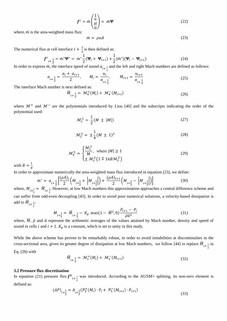
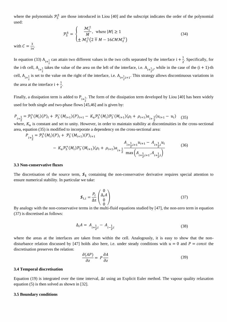
The initial pressure and temperature profiles along the tapered well are given in Figures 3 and 4 respectively. The

relatively low pressure at the bottom of the well (ca. 38 bar) means that the CO2 remains in the gaseous phase in the

first 400 m along the well, following which transition to the dense or liquid phase takes place (as indicated by the

vertical dashed lines).

Figure 3: The initial pressure profile along the well (origin corresponds to the top of the well).

Figure 4: The initial temperature profile along the well (origin corresponds to the top of the well).

Figure 5 shows the variations of the CO2 pressure and temperature at the top of the well as a function of time during

the linear ramping up injection from 0 to 33.5 kg/s over min 300 s (case 1A). The feed CO2 stream pressure and

temperature are 115 bar and 278.15 K respectively. Figure 6 shows the same transient profiles but for the higher feed

temperature of 283.15 K (case 1B) representing its prior heating. For both of the above initial conditions, the injected

CO2 is in the dense phase and remains so for the entire time frame (500 s) under consideration.

Vap

ou

r p

has

e

Den

se p

has

e

Vap

ou

r p

has

e

Figure 5: Transient pressure and temperature profiles at the top of the well for the fast injection ramping rate, case 1A (feed

temperature 278.15 K). The vertical dashed line indicates the time (300 s) at which the injection flow rate reaches its peak value of

33.5 kg/s.

Figure 6: Transient pressure and temperature profiles at the wellhead for the fast injection ramping rate; case 1B (feed temperature

283.15 K). The vertical dashed line indicates the time (300 s) at which the injection flow rate reaches its peak value of 33.5 kg/s.

As it may be observed, in both cases an initial rapid depressurisation and cooling is followed by more rapid recoveries

with the maximum values occurring at or shortly after the time (300 s) at which the injection rate reaches its peak

value (33.5 kg/s). Also, whilst the temperature remains relatively constant thereafter, a secondary modest (ca. 5 bar)

drop in the fluid pressure is obtained. As expected, the lower the feed temperature, the lower the minimum

temperature attained. In the case of the feed temperature of 278.15 K, the lowest temperature reached at the top of the

well is 265 K (case 1A). This compares with the slightly higher minimum temperature of 267.5 K for the feed

temperature of 283.15 K (case 1B). Given that both of these minimum temperatures are below the freezing point for

water, the presence of an appreciable amount of water in either the CO2 stream or the well would pose the risk of

blockage due to ice formation at the wellhead some 180 s after the injection process has commenced.

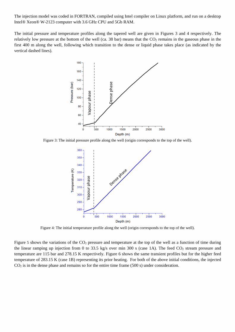
Figure 7 shows the CO2 hydrate phase diagram [53]. The dark grey region (V-I-H) represents the conditions at which

CO2 hydrate is stable together with gaseous CO2 and water ice (below 273.15 K). Table 2 shows the minimum CO2

temperatures at the wellhead and the corresponding pressures for the six test scenarios (see Table 1).

Figure 7: CO2 hydrate phase diagram [53] *

*permission to reproduce has been granted by the author.

Table 2: Lowest wellhead pressures and temperatures predicted for the examined cases

Simulation

case

Inlet

Temp

(K)

Time at

peak flow

rate (s)

Lowest

wellhead

pressure

(bar)

Lowest

wellhead

Temp

(K)

1A 278.15 300 28 265

1B 283.15 300 30 267.5

2A 278.15 1800 24 258.5

2B 283.15 1800 26.5 261.5

3A 278.15 7200 20.5 252

3B 283.15 7200 22 256

Reference to Figure 7 along with the data presented in Table 2 indicates that hydrate formation is unlikely at the

prevailing injection conditions.

Figure 8 and 9 respectively present the wellhead pressure and temperature transient profiles for the longer injection

ramping up durations of 30 min (1800 s) and 2 h (7200 s). The feed temperature in both cases is 278.15 K (cases 2A

and 3A). The observed trends in pressure and temperature are similar to those for the shorter ramping-up period with

the exception of being more in concert with one another as compared to the faster pressure ramping scenarios. The

latter is consistent with the longer opportunity for CO2 to attain thermal and pressure equilibration along the injection

well. For the medium injection rate (Figure 8), the termination of the temperature recoveries closely coincides with the

time at which the peak injection rate is reached. In the case of the long injection rate however, thermal stabilisation

occurs some 1800 s later. Most importantly, the longer the injection ramping up period, the lower is the minimum CO2

temperature reached at the wellhead thus increasing the risk of wellhead blockage due to ice formation. The minimum

temperature of ca. 252 K (21oC below the freezing point for water) is observed for case 3-A (Figure 9) corresponding

to an injection ramping-up period and temperature of 7200 s and 278.15 K respectively.

Figure 8: Transient pressure and temperature profiles at the top of the well for the medium injection ramping rate, case 2-A (feed

temperature = 278.15 K). The vertical dashed line indicates the time (1800 s) at which the injection flow rate reaches its peak

value of 33.5 kg/s.

Figure 9: Transient pressure and temperature profiles at the top of the well for the slow injection ramping rate, case 3-A (feed

temperature = 278.15 K). The vertical dashed line indicates the time (7200 s) at which the injection flow rate reaches its peak

value of 33.5 kg/s.

Interestingly, as well as being more pronounced in the magnitude of their drops, the pressure and temperature profiles

of cases 2-A (Figure 8) and 3-A (Figure 9) are in better concert with one another as compared to the faster pressure

ramping scenarios (Figures 5 and 6). Also, for case 3-A (Figure 9) at 7200 s, where the linear ramp-up injection

reaches the peak flow rate, neither the pressure nor the temperature immediately stabilise.

Figures 10 to Figure 12 respectively represent the variations of pressure and temperature at the bottom of the well as a

function of time for the fast (Figure 10; case 1-A), medium (Figure 11: case 2-A) and slow (Figure 12: case 3-A)

injection ramping strategies. The lower feed temperature of 278.15 K is assumed in all cases. As expected, the bottom

well pressure increases as the CO2 injection proceeds reaching a maximum value ca. 197 bar. Interestingly, for the

medium (Figure 11) and the slow-injection ramping rates (Figure 12), the well bottom pressure reaches its maximum

constant value at or soon after the time at which the peak injection rates are attained (1800 s and 7200 s). However in

the case of the fast injection ramping up (Figure 10), the pressure at the bottom of the well keeps increasing, albeit by

a modest amount, well after the maximum injection rate has been reached.

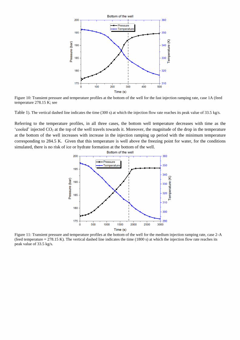
Figure 10: Transient pressure and temperature profiles at the bottom of the well for the fast injection ramping rate, case 1A (feed

temperature 278.15 K; see

Table 1). The vertical dashed line indicates the time (300 s) at which the injection flow rate reaches its peak value of 33.5 kg/s.

Referring to the temperature profiles, in all three cases, the bottom well temperature decreases with time as the

‘cooled’ injected CO2 at the top of the well travels towards it. Moreover, the magnitude of the drop in the temperature

at the bottom of the well increases with increase in the injection ramping up period with the minimum temperature

corresponding to 284.5 K. Given that this temperature is well above the freezing point for water, for the conditions

simulated, there is no risk of ice or hydrate formation at the bottom of the well.

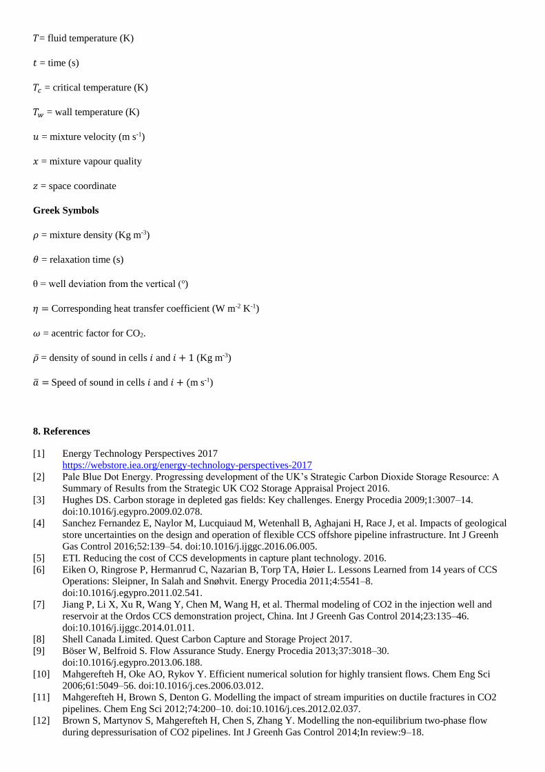
Figure 11: Transient pressure and temperature profiles at the bottom of the well for the medium injection ramping rate, case 2-A

(feed temperature = 278.15 K). The vertical dashed line indicates the time (1800 s) at which the injection flow rate reaches its

peak value of 33.5 kg/s.

Figure 12: Transient pressure and temperature profiles at the bottom of the well for the slow injection ramping rate, case 3-A (feed

temperature = 278.15 K). The vertical dashed line indicates the time (7200 s) at which the injection flow rate reaches its peak

value of 33.5 kg/s.

Finally Figure 13 shows a comparison of the simulated wellhead transient temperature profiles at the three injection

ramping up durations of 5 min (300 s), 30 min (1800 s) and 2 h (7200 s). The injection temperature and pressure are

276 K and 115 bar respectively. The solid lines represent the simulated data generated using the present model. The

dotted lines on the other hand show the predicted data reproduced from the Peterhead CCS project report [29] for CO2

injection into the depleted Golden Eye Reservoir using the commercial software, OLGA [26].

Figure 13. A comparison of the present model’s predictions for the well head temperature for the three ramping up injection rates

against those obtained using the commercial software, OLGA [26].

As it may be observed, both sets of simulations produce very similar trends; the initial rapid drop in temperature upon

the injection of CO2 is followed by a rapid recovery. The magnitude and the duration of the drop in temperature both

increase with increase in the injection ramping up duration. Also, the slower the injection ramping up rate, the longer

it takes for the fluid temperature to recover. Remarkably all three injection ramping up rates indicate minimum

temperatures falling well below zero oC indicating the risk of well blockage due to ice formation in the event of the

presence of appreciable amounts of water as well as the possibility of well bore fracture due to thermal shocking. This

risk increases as the injection ramping up rate increases. As for the finite disagreement between the predictions

between the two sets of simulations, it is difficult to draw any plausible conclusions given the absence of the detailed

pertaining theory, in particular the formulation of the boundary conditions at the wellhead and the reservoir along with

their implementation into the flow model capable of handling a time variant feed rate in the OLGA software.

5. Conclusion

As part of the challenge in combating global warming, depleted gas fields present ideal locations for storing the huge

quantities of CO2 captured from fossil fuel power plants and various energy intensive industrial emitters.

A significant expansion induced cooling of the high pressure CO2 arriving at the top of the low pressure wellhead

leading to the storage reservoir poses a number of potential hazards, including; well blockage, thermal shocking of

the well bore steel lining and a reduction in the effective storage capacity. As such, the controlled gradual expansion

of the CO2 at the point of injection into the well balancing the requirement to minimise the temperature trop whilst

ensuring maximum injection rate during the start-up injection is fundamentally important.

In this paper, we presented the development, testing and verification of a rigorous mathematical model for simulating

the highly transient flow and heat transfer effects taking place throughout the well bore during the start-up injection of

CO2 into highly depleted gas reservoirs.

Through the development and integration of the appropriate boundary conditions at the wellhead, the well bottom

(reservoir permeability) and taking into account the detailed well bore properties such as its heat transfer

characteristics and the surrounding core, well tapering and deviation from the horizontal, our model can be used as

useful practical engineering tool for determining the optimum injection ramping up rates.

Based on the application of the injection model simulating the injection of CO2 in a real offshore depleted gas field in

the North Sea, we make the following important observations for three selected nominal injection ramping up rates

representing slow, medium and slow injection scenarios;

i) in all cases tested, the temperature of expanded CO2 at the wellhead drops well below zero oC

representing the risk of well blockage due to ice formation in the event of the presence of an appreciable

amount of water and well bore fracture due to thermal shocking. However, well blockage due to hydrate

formation proved unlikely;

ii) remarkably, the magnitude of the temperature drop increases with decrease in the injection ramping up

rate. This means that slower injection ramping up rate gives rise to a higher risk of well blockage. The

above observation is consistent with the published literature;

iii) as expected the preheating of the CO2 prior to its injection reduces the risk of ice formation. However, the

corresponding energy and hence cost implications will most likely not make this a viable option

especially given the significant quantities of CO2 being injected in practice (typically, millions of tonnes

to reach full reservoir capacity);

iv) in none of the three test cases examined does the well bottom temperature drops below zero oC indicating

minimal risk of the blockage of the well bore bottom perforations.

In conclusion, it is important to point out that the above observations are based on the application of the model

developed to the particular, albeit realistic test case examined in the present study. As such the findings should not be

considered as universally applicable to all cases involving injection of CO2 into depleted gas reservoirs. Each injection

scenario should be investigated based on the prevailing conditions. Certainly, this study shows that the choice of the

injection ramping up rate has a profound impact on the highly transient temperature and pressure profiles incurring

during the start-up injection process and the subsequent risks. The mathematical model presented in this work, once

translated into a robust computational software, can be used as a valuable tool by engineers to determine the optimum

injection ramping up rates into depleted gas reservoirs. This will contribute to accelerating the role out of CCS in

transitioning the CO2 emitting energy intensive industries onto a pathway consistent with the quest to limit the

increase in the global average temperatures.

6. Acknowledgement

The authors are grateful to the UK Carbon Capture and Storage Research Centre for the funding of this work through

the Flexible funding Call 2 C2-183.

7. NomenclatureA= well bore cross sectional Area (m2)

�̃� = minimum pressure required for the flow to start from the well into the reservoir (Pa)

�̃� = site-specific dimensional constant (Pa s Kg-1)

�̃� = site-specific dimensional constant (Pa s Kg-2)

𝑐𝑝 = heat capacity at constant pressure (J K-1)

𝐷𝑝 = internal diameter of the pipe (m)

𝐸 = specific total energy (J Kg-1)

𝑒 = specific internal energy (J Kg-1)

𝐹 = viscous friction force

𝑓𝑤 = Fanning friction factor

𝑔 = gravitational acceleration (m s -2)

𝐻 = total enthalpy of the fluid (kJ kg-1)

𝑘= fluid thermal conductivity (W m-1 K-1)

𝜅 = heat conductivity (W m-1 K-1)

𝑀 = instantaneous mass flow rate at the bottom hole (kg s-1)

𝑚𝑙 = meta-stable(super-heated) liquid phase

�̇� = area-weighted mass flux (kg s−1 m−2)

ℳ= Mach number

�̅�= arithmetic averages of the values attained by Mach number

𝑃= Mixture pressure (bar)

𝑃𝐵𝐻𝐹 = instantaneous bottom hole pressure (bar)

𝑃𝑐 = critical pressure (bar)

𝑃𝑟 = Fluid Prandtl number

𝑃𝑟𝑒𝑠 = reservoir static pressure (bar)

𝑅𝑒 = Reynolds number

𝑄 = heat flux (W m−2)

𝑠𝑣 = saturated vapour phase

𝑇= fluid temperature (K)

𝑡 = time (s)

𝑇𝑐 = critical temperature (K)

𝑇𝑤 = wall temperature (K)

𝑢 = mixture velocity (m s-1)

𝑥 = mixture vapour quality

𝑧 = space coordinate

Greek Symbols

𝜌 = mixture density (Kg m-3)

𝜃 = relaxation time (s)

θ = well deviation from the vertical (o)

𝜂 = Corresponding heat transfer coefficient (W m-2 K-1)

𝜔 = acentric factor for CO2.

�̅� = density of sound in cells 𝑖 and 𝑖 + 1 (Kg m-3)

�̅� = Speed of sound in cells 𝑖 and 𝑖 + (m s-1)

8. References

[1] Energy Technology Perspectives 2017

https://webstore.iea.org/energy-technology-perspectives-2017

[2] Pale Blue Dot Energy. Progressing development of the UK’s Strategic Carbon Dioxide Storage Resource: A

Summary of Results from the Strategic UK CO2 Storage Appraisal Project 2016.

[3] Hughes DS. Carbon storage in depleted gas fields: Key challenges. Energy Procedia 2009;1:3007–14.

doi:10.1016/j.egypro.2009.02.078.

[4] Sanchez Fernandez E, Naylor M, Lucquiaud M, Wetenhall B, Aghajani H, Race J, et al. Impacts of geological

store uncertainties on the design and operation of flexible CCS offshore pipeline infrastructure. Int J Greenh

Gas Control 2016;52:139–54. doi:10.1016/j.ijggc.2016.06.005.

[5] ETI. Reducing the cost of CCS developments in capture plant technology. 2016.

[6] Eiken O, Ringrose P, Hermanrud C, Nazarian B, Torp TA, Høier L. Lessons Learned from 14 years of CCS

Operations: Sleipner, In Salah and Snøhvit. Energy Procedia 2011;4:5541–8.

doi:10.1016/j.egypro.2011.02.541.

[7] Jiang P, Li X, Xu R, Wang Y, Chen M, Wang H, et al. Thermal modeling of CO2 in the injection well and

reservoir at the Ordos CCS demonstration project, China. Int J Greenh Gas Control 2014;23:135–46.

doi:10.1016/j.ijggc.2014.01.011.

[8] Shell Canada Limited. Quest Carbon Capture and Storage Project 2017.

[9] Böser W, Belfroid S. Flow Assurance Study. Energy Procedia 2013;37:3018–30.

doi:10.1016/j.egypro.2013.06.188.

[10] Mahgerefteh H, Oke AO, Rykov Y. Efficient numerical solution for highly transient flows. Chem Eng Sci

2006;61:5049–56. doi:10.1016/j.ces.2006.03.012.

[11] Mahgerefteh H, Brown S, Denton G. Modelling the impact of stream impurities on ductile fractures in CO2

pipelines. Chem Eng Sci 2012;74:200–10. doi:10.1016/j.ces.2012.02.037.

[12] Brown S, Martynov S, Mahgerefteh H, Chen S, Zhang Y. Modelling the non-equilibrium two-phase flow

during depressurisation of CO2 pipelines. Int J Greenh Gas Control 2014;In review:9–18.

doi:10.1016/j.ijggc.2014.08.013.

[13] Oldenburg CM. Joule-Thomson cooling due to CO2 injection into natural gas reservoirs. Energy Convers

Manag 2007;48:1808–15. doi:10.1016/j.enconman.2007.01.010.

[14] André L, Audigane P, Azaroual M, Menjoz A. Numerical modeling of fluid-rock chemical interactions at the

supercritical CO2-liquid interface during CO2 injection into a carbonate reservoir, the Dogger aquifer (Paris

Basin, France). Energy Convers Manag 2007;48:1782–97. doi:10.1016/j.enconman.2007.01.006.

[15] Oldenburg CM, Moridis GJ, Spycher N, Pruess K. EOS7C Version 1.0: TOUGH2 Module for Carbon Dioxide

or Nitrogen inNatural Gas (Methane) Reservoirs. Berkeley, CA: 2004. doi:10.2172/878525.

[16] Goodarzi S, Settari A, Zoback MD, Keith D. Thermal Aspects of Geomechanics and Induced Fracturing in

CO2 Injection With Application to CO2 Sequestration in Ohio River Valley. SPE Int Conf CO2 Capture,

Storage, Util 2010;2. doi:10.2118/139706-MS.

[17] Linga G, Lund H. A two-fluid model for vertical flow applied to CO2 injection wells. Int J Greenh Gas Control

2016;51:71–80. doi:10.1016/j.ijggc.2016.05.009.

[18] Span R, Wagner W. A New Equation of State for Carbon Dioxide Covering the Fluid Region from the Triple-

Point Temperature to 1100 K at Pressures up to 800 MPa. J Phys Chem Ref Data 1996;25:1509.

doi:10.1063/1.555991.

[19] Li X, Xu R, Wei L, Jiang P. Modeling of wellbore dynamics of a CO2 injector during transient well shut-in

and start-up operations. Int J Greenh Gas Control 2015;42:602–14. doi:10.1016/j.ijggc.2015.09.016.

[20] Lu M, Connell LD. Non-isothermal flow of carbon dioxide in injection wells during geological storage. Int J

Greenh Gas Control 2008;2:248–58. doi:10.1016/S1750-5836(07)00114-4.

[21] Paterson L, Lu M, Connell L, Ennis-King J. Numerical Modeling of Pressure and Temperature Profiles

Including Phase Transitions in Carbon Dioxide Wells. SPE Annu Tech Conf Exhib Denver, Color USA, Sept

21-24 2008. doi:10.2118/115946-MS.

[22] Lindeberg E. Modelling pressure and temperature profile in a CO2 injection well. Energy Procedia

2011;4:3935–41. doi:10.1016/j.egypro.2011.02.332.

[23] Pan L, Webb SW, Oldenburg CM. Analytical solution for two-phase flow in a wellbore using the drift-flux

model. Adv Water Resour 2011;34:1656–65. doi:10.1016/j.advwatres.2011.08.009.

[24] Lu M, Connell LD. The transient behaviour of CO2 flow with phase transition in injection wells during

geological storage – Application to a case study. J Pet Sci Eng 2014;124:7–18.

doi:10.1016/j.petrol.2014.09.024.

[25] Tollak S, Bernstone C, Clausen S, Koeijer G De, Mølnvik MJ. Combining thermodynamic and fluid flow

modelling for CO 2 flow assurance 2013;00.

[26] Bendiksen KH, Maines D, Moe R, Nuland S. The Dynamic Two-Fluid Model OLGA: Theory and Application.

SPE Prod Eng 1991;6:171–80. doi:10.2118/19451-PA.

[27] Li X, Li G, Wang H, Tian S, Song X, Lu P, et al. International Journal of Greenhouse Gas Control A unified

model for wellbore flow and heat transfer in pure CO 2 injection for geological sequestration , EOR and

fracturing operations. Int J Greenh Gas Control 2017;57:102–15. doi:10.1016/j.ijggc.2016.11.030.

[28] Lund H, Torsæter M, Munkejord ST. Study of Thermal Variations in Wells During Carbon Dioxide Injection.

Soc Pet Eng - SPE Bergen One Day Semin 2015 2015;31:327–37. doi:10.2118/173864-PA.

[29] Shell. Peterhead CCS Project. 2015.

[30] Lu M, Connell LD. Transient, thermal wellbore flow of multispecies carbon dioxide mixtures with phase

transition during geological storage. Int J Multiph Flow 2014;63:82–92.

doi:10.1016/j.ijmultiphaseflow.2014.04.002.

[31] Raza A, Gholami R, Rezaee R, Bing CH, Nagarajan R, Hamid MA. Well selection in depleted oil and gas

fields for a safe CO2 storage practice: a case study from Malaysia. Petroleum 2016.

doi:10.1016/j.petlm.2016.10.003.

[32] Brown S, Martynov S, Mahgerefteh H, Proust C. A homogeneous relaxation flow model for the full bore

rupture of dense phase CO2 pipelines. Int J Greenh Gas Control 2013;17:349–56.

doi:10.1016/j.ijggc.2013.05.020.

[33] Brown S, Martynov S, Mahgerefteh H. Simulation of two-phase flow through ducts with discontinuous cross-

section. Comput Fluids 2015;120:46–56. doi:10.1016/j.compfluid.2015.07.018.

[34] Downar-Zapolski P, Bilicki Z, Bolle L, Franco J. The non-equilibrium relaxation model for one-dimensional

flashing liquid flow. Int J Multiph Flow 1996;22:473–83. doi:10.1016/0301-9322(95)00078-X.

[35] Chen NH. An Explicit Equation for Friction Factor in Pipe. Ind Eng Chem Fundam 1979;18:296–7.

doi:10.1021/i160071a019.

[36] Wood DA. Metaheuristic profiling to assess performance of hybrid evolutionary optimization algorithms

applied to complex wellbore trajectories. J Nat Gas Sci Eng 2016;33:751–68. doi:10.1016/j.jngse.2016.05.041.

[37] Chabook M, Al-Ajmi A, Isaev V. The role of rock strength criteria in wellbore stability and trajectory

optimization. Int J Rock Mech Min Sci 2015;80:373–8. doi:10.1016/j.ijrmms.2015.10.003.

[38] Dittus FW, Boelter LMK. Heat Transfer in Automobile Radiators 1930;2:443.

[39] Peng D-Y, Robinson DB. A New Two-Constant Equation of State. Ind Eng Chem Fundam 1976;15:59–64.

doi:10.1021/i160057a011.

[40] Diamantonis NI, Economou IG. Evaluation of statistical associating fluid theory (SAFT) and perturbed chain-

SAFT equations of state for the calculation of thermodynamic derivative properties of fluids related to carbon

capture and sequestration. Energy and Fuels 2011;25:3334–43. doi:10.1021/ef200387p.

[41] Poling BE, Prausnitz JM, O’Connell JP. The properties of gases and liquids. McGraw-Hill; 2001.

[42] Liou MS. A sequel to AUSM, Part II: AUSM+-up for all speeds. J Comput Phys 2006;214:137–70.

doi:10.1016/j.jcp.2005.09.020.

[43] Liou M. A Sequel to AUSM: AUSM. J Comput Phys 1996;129:364–82. doi:10.1006/jcph.1996.0256.

[44] Niu Y-Y, Lin Y-C, Chang C-H. A further work on multi-phase two-fluid approach for compressible multi-

phase flows. Int J Numer Methods Fluids 2008;58:879–96.

[45] Paillère H, Corre C, García Cascales JR. On the extension of the AUSM+ scheme to compressible two-fluid

models. Comput Fluids 2003;32:891–916. doi:10.1016/S0045-7930(02)00021-X.

[46] Robbins DJ, Cant RS, Gladden LF. Development of accurate, robust liquid equations of state for multi-phase

CFD simulations with a modified AUSM+-up scheme. Comput Fluids 2013;77:166–80.

doi:10.1016/j.compfluid.2013.01.031.

[47] Liou MM-S, Nguyen L, Theofanous TG, Chang CC-H, Nguyen L, Theofanous TG. How to Solve

Compressible Multifluid Equations: a Simple, Robust, and Accurate Method. AIAA J 2008;46:2345–56.

doi:10.2514/1.34793.

[48] LeVeque RJ. Finite Volume Methods for Hyperbolic Problems: Cambridge: Cambridge University Press;

2002. doi:10.1017/CBO9780511791253.

[49] Thompson KW. Time dependent boundary conditions for hyperbolic systems. J Comput Phys 1987;68:1–24.

doi:10.1016/0021-9991(87)90041-6.

[50] Thompson KW. Time-dependent boundary conditions for hyperbolic systems, {II}. J Comput Phys

1990;89:439–61. doi:10.1016/0021-9991(90)90152-Q.

[51] Cotton A, Gray L, Maas W. Learnings from the Shell Peterhead CCS Project Front End Engineering Design.

Energy Procedia 2017;114:5663–70. doi:10.1016/J.EGYPRO.2017.03.1705.

[52] Mahgerefteh H, Rykov Y, Denton G. Courant, Friedrichs and Lewy (CFL) impact on numerical convergence

of highly transient flows. Chem Eng Sci 2009;64:4969–75. doi:10.1016/J.CES.2009.08.002.

[53] Genov GY. Physical processes of the CO2 hydrate formation and decomposition at conditions relevant to Mars

2005.

kgkg