Modelling pupils’ absenteeism: Emerging policy issues … from the... · Modelling pupils’...
29
1 Modelling pupils’ absenteeism: Emerging policy issues from SACMEQ projects Hungi, N. (Australian Council for Educational Research, Sydney) Abstract This study employed a multilevel technique to examine pupil- and school-level factors that influence absenteeism rates among Standard 6 primary school pupils in Kenya. The data used in this study were collected as part of Southern Africa Consortium for Monitoring Educational Quality (SACMEQ) II project in 2002 from 3,299 pupils in 185 schools in eight provinces in Kenya. At the individual level, results show that pupil's age, pupil's home background (SES), number of meals eaten by pupil per week and corrections of the homework given to the pupil significantly influence absenteeism rates in Kenya. At the group level, results show that working places in class (for sitting and writing) and school geographical location (province) significantly influence absenteeism in Kenya. Policy implications of these results are discussed. 1 Introduction Absenteeism has been associated with undesirable outcomes, such as poor academic achievement and low school internal efficiency (high repetition rates and high dropout rates) and discipline problems. Obviously, students who are regular absentees receive fewer hours of instruction and therefore are highly likely to achieve at a lower level compared to the rest of their classmates. It is not hard to see that frequent absenteeism could lead to less engagement in schoolwork and therefore less motivation to continue with schooling. A number of research studies in developed countries have reported significant relationships between absenteeism and poor academic achievement (e.g. Monk and Ibrahim,
Transcript of Modelling pupils’ absenteeism: Emerging policy issues … from the... · Modelling pupils’...

1
Modelling pupils’ absenteeism: Emerging policy issues from
SACMEQ projects
Hungi, N. (Australian Council for Educational Research, Sydney)
Abstract
This study employed a multilevel technique to examine pupil- and school-level factors
that influence absenteeism rates among Standard 6 primary school pupils in Kenya. The data
used in this study were collected as part of Southern Africa Consortium for Monitoring
Educational Quality (SACMEQ) II project in 2002 from 3,299 pupils in 185 schools in eight
provinces in Kenya. At the individual level, results show that pupil's age, pupil's home
background (SES), number of meals eaten by pupil per week and corrections of the homework
given to the pupil significantly influence absenteeism rates in Kenya. At the group level,
results show that working places in class (for sitting and writing) and school geographical
location (province) significantly influence absenteeism in Kenya. Policy implications of these
results are discussed.
1 Introduction
Absenteeism has been associated with undesirable outcomes, such as poor academic
achievement and low school internal efficiency (high repetition rates and high dropout rates)
and discipline problems. Obviously, students who are regular absentees receive fewer hours
of instruction and therefore are highly likely to achieve at a lower level compared to the rest
of their classmates. It is not hard to see that frequent absenteeism could lead to less
engagement in schoolwork and therefore less motivation to continue with schooling.
A number of research studies in developed countries have reported significant
relationships between absenteeism and poor academic achievement (e.g. Monk and Ibrahim,
2
1984; Moore, 2004; Reynolds and Walberg, 1991; Rumberger and Larson, 1998). For
example, Rumberger and Larson (1998), analyzing data from grade 7 (N = 746) and grade 9
(N = 663) students from a large middle school system in California in the United States,
found that students with high rates of absenteeism had worse grades than students with
moderate rates of absenteeism. Rumberger and Larson also found that students who were
absent more than 25 per cent of the time were more than twice as likely to leave school early
as were students who were absent less than 15 per cent of the time.
There is also research evidence from developing countries that links absenteeism with
low academic achievement. For example, Hungi (2004a), using data from 36,476 grade 5
pupils in 7,221 classes in 3,635 schools in Vietnam, found that absenteeism had significant
negative effects on pupil achievement in reading and mathematics both at the individual and
the class-level. This indicated that high absenteeism rates at the class-level affected regular
attendees within the class as well. In the Kenya context at the primary school level, findings
from Southern Africa Consortium for Monitoring Educational Quality (SACMEQ) II projects
indicate that pupils, who were never (or were rarely) absent from school were more likely to
achieve better in reading and mathematics than those pupils who were frequently absent from
school (Hungi, 2004b). In the SACMEQ I project, Nzomo, Kariuki and Guantai (2001) found
that the average absenteeism rate among Standard 6 pupils in Kenya was about two days per
month. Nzomo et al. (2001) contended that the performance of pupils was greatly affected by
absenteeism.
The data for this study were collected as part of the SACMEQ II project in 2002 from
3,299 pupils in 185 primary schools in eight provinces in Kenya. There are two main
purposes of the current study. The first purpose is to identify pupil and school-related factors
that influence absenteeism among Standard 6 pupils in Kenya. The second purpose is to
develop a multilevel model that could be used to explain some of the variance associated with

3
absenteeism among Standard 6 pupils in Kenya. The multilevel technique employed in this
study has been used by Rothman (2000) in his analysis of absenteeism among primary school
pupils in South Australia.
The structure of this article is as follows. A section is included in which some
preliminary analyses of the data are reported. Two sections are provided in which the
hypothesized multilevel model is described and the specifications of this model are outlined.
The multilevel analysis is described and, finally, sections containing the results of the
analyses are presented and discussed.
2 Some preliminary data analyses
As mentioned in the introduction, data for this study was collected as part of the
SACMEQ II project in 2002. A wide range of information about characteristics of pupils,
classes, teachers and schools was collected. The variables examined in this study are those
variables identified as potential predictors of absenteeism following sound reasoning and
research findings from studies in other countries.
The pupils were asked how many days they were absent from school in the previous
month. The number of days absent ranged from 0 — 21 days and the average number of days
absent was about two days. The percentages of pupils who said they were absent for zero,
one, two, three and four days were 48.6, 13.5, 10.1, 8.6 and 4.8 respectively. This means that
85.6 per cent of the pupils were absent from school for four days or less. In other words, 14.4
per cent of the pupils were absent for at least five days (i.e. one school week) in the previous
month. The analyses reported in this paper do not distinguish between absenteeism with
permission from school authorities and absenteeism without permission from school
authorities.

4
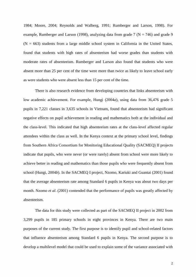
A breakdown of the absenteeism rates by some of the pupil and school level variables
examined in this study has been given in Table 1. It should be noted that, in the estimation of
the statistics shown in Table 1, pupil weights and the clustering nature of these data (i.e.
pupils nested within schools) were taken into consideration using AM (AIR and Cohen, 2003)
computer software. However, in the estimation of the statistics in Table 1, the distribution
nature of Days absent data (Poisson distribution) was not taken into consideration and the data
were assumed to be normally distributed.
<Insert Table 1 about here>
The results in Table 1 shows that boys' mean absenteeism rate (1.98) closely follows
that of girls' (1.94), which indicates that pupil's sex may not be a factor influencing
absenteeism rate among Standard 6 pupils in Kenya. The results in Table 1 indicate that the
variable ‘Home possession level’ could be a factor influencing absenteeism rate. This is
because the mean absenteeism rate of pupils from poor homes (2.23) is noticeably larger than
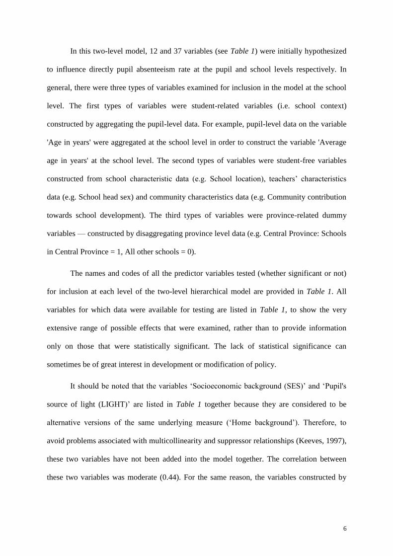
that of pupils from rich homes (1.56). Similarly, ‘Pupil source of light’ could also be a factor
related to absenteeism rate according to the results in Table 1 and Figure 1.
Figure 1 is a box plot of the absenteeism rate by ‘Pupil source of light’ data plotted
using SPSS version 10.0 for Windows. When interpreting results obtained using SPSS version
10.0 for Windows, it should be noted that this software does not allow for the clustering
nature of the data and therefore gives misleadingly small standard errors when used with
multilevel data. Nevertheless, the plot in Figure 1 provides some evidence that there could be
significant differences between the absenteeism rate of pupils from homes with electric
lighting and the absenteeism rate of pupils from homes with fire lighting or with no sources of

5
lighting. A similar plot for Province data (Figure 2) indicate that there could be significant
differences between the absenteeism rate of pupils attending schools in Rift Valley Province
and the absenteeism rate of pupils attending schools in say Nairobi, Eastern and Central
Provinces.
<Insert Figure 1 about here>
<Insert Figure 2 about here>
As a word of caution, the multilevel analyses that are reported in later sections of this
article should not be expected to give identical results to the results in Table 1. This is because
some of the differences reported above might not survive when the multilevel nature of the
data and the distributional nature of the data have been taken into account in the analyses.
Importantly, the results of the multilevel analyses are expected to give a better picture of the
effects of various factors on absenteeism rate compared with the results obtained using the
approach described above.
3 Hypothesized model
When dealing with multilevel data such as the data in this study, the appropriate
procedure is to formulate multilevel models, "which enable the testing of hypotheses about
effects occurring within each level and the interrelations among them" (Raudenbush and
Bryk, 1994, p. 2590). Consequently, in this study, a two-level model was hypothesized to
enable the testing of hypotheses about the factors influencing absenteeism rate among
Standard 6 pupils in Kenya. The hierarchical structure of this model was obtained using
pupils at level-1 and schools at level-2. In other words, pupils were nested within schools.
6
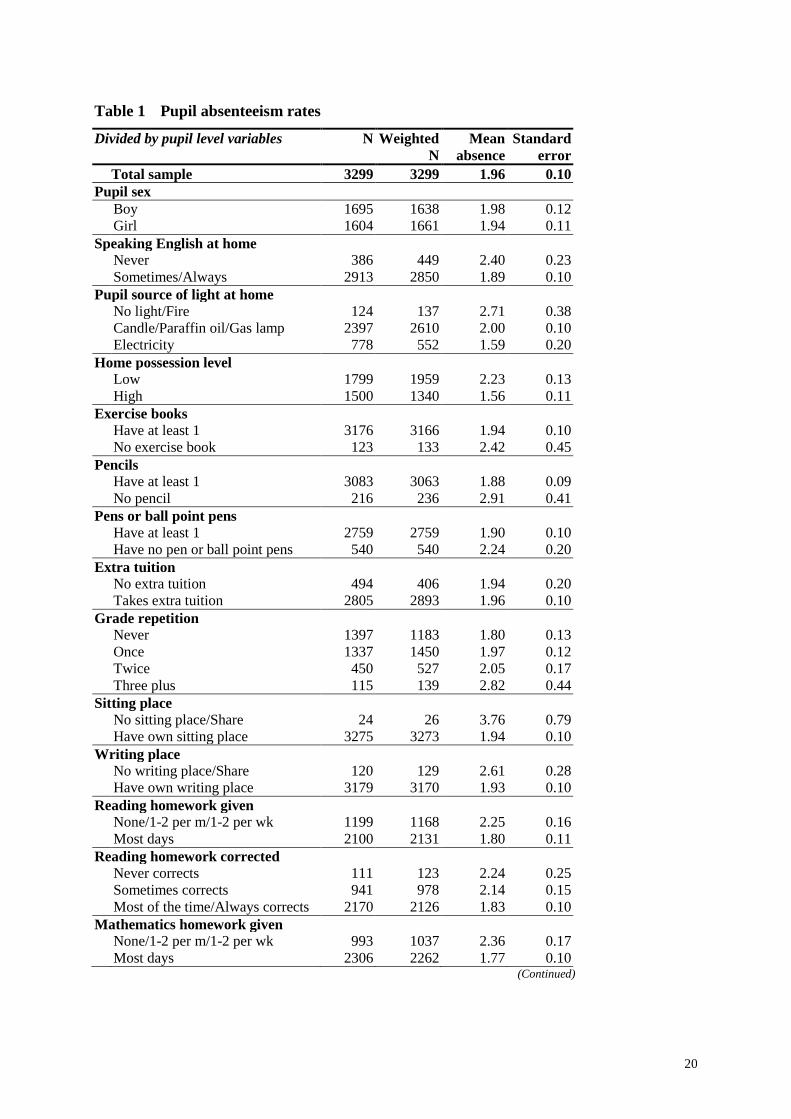
In this two-level model, 12 and 37 variables (see Table 1) were initially hypothesized
to influence directly pupil absenteeism rate at the pupil and school levels respectively. In
general, there were three types of variables examined for inclusion in the model at the school
level. The first types of variables were student-related variables (i.e. school context)
constructed by aggregating the pupil-level data. For example, pupil-level data on the variable
'Age in years' were aggregated at the school level in order to construct the variable 'Average
age in years' at the school level. The second types of variables were student-free variables
constructed from school characteristic data (e.g. School location), teachers’ characteristics
data (e.g. School head sex) and community characteristics data (e.g. Community contribution
towards school development). The third types of variables were province-related dummy
variables — constructed by disaggregating province level data (e.g. Central Province: Schools
in Central Province = 1, All other schools = 0).
The names and codes of all the predictor variables tested (whether significant or not)
for inclusion at each level of the two-level hierarchical model are provided in Table 1. All
variables for which data were available for testing are listed in Table 1, to show the very
extensive range of possible effects that were examined, rather than to provide information
only on those that were statistically significant. The lack of statistical significance can
sometimes be of great interest in development or modification of policy.
It should be noted that the variables ‘Socioeconomic background (SES)’ and ‘Pupil's
source of light (LIGHT)’ are listed in Table 1 together because they are considered to be
alternative versions of the same underlying measure (‘Home background’). Therefore, to
avoid problems associated with multicollinearity and suppressor relationships (Keeves, 1997),
these two variables have not been added into the model together. The correlation between
these two variables was moderate (0.44). For the same reason, the variables constructed by
7
aggregated pupil-level data on these two variables at the school level (SES_2 and LIGHT_2)
are listed together in Table 1.
4 Specification of the model
The distribution of the outcome variable (‘Days absent’) followed a Poisson
distribution (see Figure 3). When the distribution of the outcome variable is Poisson, HLM5
(Raudenbush, Bryk, Cheong and Congdon, 2000a) uses log link function. Thus, for this study,
and following the notations and arguments presented by Raudenbush and Bryk (2002), the
two-level Poisson model for the estimation of pupil absenteeism rate, can be described as
follows.
Level-1 model
At the micro-level, the log of pupil absenteeism rate is modelled as a function of
school mean and pupil-level background variables:
hijhjjij X 0)log( Equation 1
where:
ij is the absenteeism rate of pupil i in school j;
j0 is the log of the mean absenteeism rate of school j;
hijX are the background characteristics of pupil i in school j; and
hj are the logs of regression coefficients associated with the pupil background
characteristics of school j.
The indices i, and j denote pupils and schools. There are
i = 1, 2, . . . , nj pupils within school j; and
j = 1, 2, . . . , J schools (in this study, J = 185);

8
For parsimony, hijhjX in Equation 1 represents the control for several relevant
independent variables )( 2211 hijhjijjijj XXX that describe pupil's background
characteristics. There are h = 1, 2, . . . , H (in this study, H = 12) independent variables which
describe student's background characteristics. Hence, for the current study, hijX represents a
combination of any of the 12 pupil-level variables listed in Table 2.
Level-2 model
At the macro-level of the model, the intake-adjusted log of absenteeism rate, j0 , is
regressed on school-level variables ( gjW ) for each school.
jgjgj uW 000000 Equation 2
where:
00 is the log of the mean absenteeism rate of all schools (grand-mean),
g0 are the logs of the slopes associated with the school-level variables; and
ju0 is a random error associated with school j.
For parsimony, gjgW00 in Equation 2 represents the control for several relevant
school-level variables )( 0002020101 gjgjj WWW that describe the school context,
school characteristics, teachers’ characteristics and community characteristics. There are g =
1, 2, . . . , G (in this study G = 37) school-level variables. Hence, for the current study gjW
represents a combination of any of the 37 school-level variables listed in Table 2.
In addition, at this level of the model each component that is associated with the pupil
background characteristics, ( hj ) is viewed as an outcome varying randomly around some
school mean ( 0h ), that is:

9
hjhhj
jj
jj
u
u
u
0
2202
1101
Equation 3
For purposes of simplicity, cross-level interaction effects have been excluded from
Equation 3 above, but in actual analyses, cross-level interaction effects were examined.
However, no cross-level interaction effects were significant in this study.
5 Method
A preliminary task in HLM analyses was to build a sufficient statistics matrix (SSM)
file. No pupils or schools were dropped due to insufficient data in the construction of this
SSM file. Consequently, the Ns in this SSM file remained as they were in the original data
files; that is, 3299 for pupils and 185 for schools.
The first step undertaken in HLM analyses was to specify the outcome variable, which
is ABSENT (‘Days absent’). The distribution of this outcome variable followed a Poisson
distribution (see Figure 3). Thus, the second step undertaken was to set up a non-linear model
(Poisson, with constant exposure) using the optional specification menu available in HLM5.
The third step undertaken was to run a null model in order to obtain the amount of variance
available to be explained at each level of the hierarchy. The null model was the simplest
model because it contained only the dependent variable (for this study, number of days
absent) and no predictor variables were specified at any level.
<Insert Table 2 about here>

10
The fourth step undertaken was to build up the pupil-level model or the so-called
‘unconditional’ model at level-1. This involved adding pupil-level predictors to the model, but
without entering predictors at the school level. The purpose of this step was to examine which
pupil-level variables had significant (p<0.05 level) effects on the outcome variables. An
approach referred to as a ‘step-up’ approach (Bryk and Raudenbush, 1992) was followed to
examine which of the pupil-level variables had a significant influence on days absent from
school in the hypothesized model. Bryk and Raudenbush (1992) recommended the step-up
approach for inclusion of variables into the model to the alternative approach referred to as
‘working-backward’ where all the possible predictors are included in the model and then the
non-significant variables are progressively eliminated from the model.
It should be noted that, in this study, all pupil-level predictor variables were grand-
mean-centred in the HLM analyses so that the intercept term would represent the average
number of days absent for the schools.
The final step in the HLM analyses involved adding the level-2 (school) predictors
into the model using the step-up strategy mentioned above. The level-2 exploratory analysis
sub-routine available in HLM5 was employed for examining the potentially significant level-2
predictors (as shown in the output) in successive HLM runs.
It is worth noting that the Poisson option of HLM5 generates two main solutions, one
for the so-called ‘unit-specific’ model, and the other referred to as the ‘population-average’
model (Raudenbush, Bryk, Cheong and Congdon, 2000b, p. 128). Raudenbush and Bryk
(2002, p.301) note that “though inferences based on these two models are often quite similar,
the models are oriented towards somewhat different research aims”.
In this study, the unit-specific model is useful if examining how differences in pupil
(or school) characteristics are related to absenteeism rate holding constant the school attended,
that is, absenteeism rate for the same kind of schools, schools sharing the same value of u0j in

11
Equation 2 above. On the other hand, the population-average model is useful when examining
how differences in pupil (or school) characteristics are related to absenteeism rate for all
schools nationwide, that is, the difference of interest averaging over all possible values of u0j
in Equation 2 (see Raudenbush et al. 2000b, pp. 128–130). For purposes of generalizing
findings across schools in Kenya, the results discussed in this study are from the population-
average model.
In addition, the Poisson option produces model-based standard errors and robust
standard errors for the population-average model. Raudenbush and Bryk (2002) have argued
that, for a given coefficient, if the model-based standard error is markedly different from the
robust standard error it gives evidence of misspecification of random effects. Consequently,
Raudenbush and Bryk have recommended comparing these two types of standard errors when
making a decision on whether to specify the regression coefficient as ‘fixed’ or ‘random’. For
this study, specifying a coefficient as fixed involves constraining it to be the same across all
schools while specifying it as random allows it to vary among schools.
6 Results and discussion
The final two-level model for days absent from school has been presented below in
equation form.
Level-1 model
ijjijjijjijjjij SESAGEHMKRMCMEALS )()()()()log( 43210
Level-2 model
jj
j
j
j
jjjjj
u
uRTVALLEYWESTERNWPLACE
4404
303
202
101
0030201000 )()()2_(

12
Equation 4
The above equation indicates that, for example, the absenteeism rate of Pupil 1 who
ate average number of meals per week was expected to be )exp( 1 times the absenteeism rate
of Pupil 2 who ate meals one standard deviation below the average number of meals per week
if all other factors were equal. By way of another example, the above equation indicates that
the absenteeism rate of Pupil 3 attending a school in Western Province was expected to be
)exp( 02 times the absenteeism rate of Pupil 4 attending a school in another province
assuming all other factors were equal.
Estimates for both the unit-specific and the population-average models have been
presented in Table 3 for the null, level-1 unconditional and final models. The multiplier
effects in Table 3 were calculated by taking the exponential (exp) of the estimated coefficient.
The descriptive statistics of the variables included in the final model have been given at the
bottom of Table 3. These descriptive statistics are from HLM analyses.
As mentioned above, discussion in this study is based on the population-average
model. Nevertheless, the unit-specific model estimates have been provided in Table 3 to allow
interested readers to make comparisons with the population-average model estimates. It can
be seen from Table 3 that, apart from the intercept, the coefficient estimates based on
population-average model follow closely those based on the unit-specific model. In addition,
the model-based standard errors follow closely the robust standard errors and therefore there
is no evidence of misspecification of random effects.
In interpreting the results in Table 3, it is worth noting that signs of coefficients
indicate directions of effects and can be interpreted meaningfully if the codings of the
variables are considered. For example, the negative coefficient for ‘Socioeconomic status’
(SES) indicates that pupils from low SES homes were estimated to have higher absenteeism

13
rates than pupils from high SES homes. The following examples illustrate the meaning of the
results presented in Table 3.
<Insert Table 3 about here>
For the null population-average model, the predicted average number of days absent
for schools is 1.90 (that is, ]64.0exp[ ) with a variance of 0.38. Thus, the intercept of the null
model shows that 95 per cent of the schools were expected to have absenteeism rates in the
interval )96.1*38.064.0exp( , which is equal to (0.57, 6.35). For the final population-
average model the intercept, 62.1)48.0exp( , is the estimated average number of days absent
for schools, controlled for Rift Valley and Western Provinces, and assuming that all schools
have pupils with the same pupil-level characteristics and that all school-level factors are equal
across schools. The 95 per cent confidence interval for the final population-average model
intercept is )96.1*29.048.0exp( , which is equal to (0.56, 4.64).
The multiplier effect [=exp(coefficient)] of a pupil-level variable is the estimated
absenteeism rate of a pupil with a mean score of that variable, which is also the estimated
change in number of days absent due to a one standard deviation change in that predictor
variable. For example, for the population-average model, if all other factors are equal,
Standard 6 pupils of average age (13.9 years) were estimated to have 1.07 times the
absenteeism rate of pupils of age one standard deviation below the mean age (that is, 13.9 -
1.6 = 12.4 years). For the dummy variable WESTERN, the multiplier effect indicates that, if
all other factors were equal, pupils attending schools in Western Province were estimated to
have exp(0.32) = 1.38 times the absenteeism rate of pupils attending schools in other
provinces in Kenya, based on the final population-average model.

14
6.1 Pupil-level model
From Table 3, it can be seen that four of the 12 pupil-level variables (listed in Table 2)
examined in this study had significant influences on days absent from school. These four
pupil-level variables were 1) Age in years, 2) Socioeconomic status, 3) Meals per week, and
4) Homework corrected.
In summary, the following effects on absenteeism were recorded among Kenyan
Standard 6 pupils when other factors were equal.
Age in years: Older pupils in Standard 6 in Kenya were estimated to have higher
absenteeism rates than their younger counterparts attending the same school. It is likely that
the older pupils felt discouraged to be in the same grade level with younger pupils. Thus,
education policy should emphasize that children should enter school at the designed age and
very few should repeat grades.
Socioeconomic status: Pupils from homes with better quality houses, many
possessions, more educated parents and who had the most learning materials had lower
absenteeism rates than pupils from homes with low quality houses, few or no possessions, less
educated parents and who had hardly any learning materials. Parents of high socioeconomic
status are often well educated and they show interest in their children learning in school and
encourage children to go to school. Such parents often provide their children with basic
learning materials, such as pens and pencils. Clearly, it is important for pupils to have basic
learning materials to go to school as well as for academic progress in general. In most cases,
poor parents cannot afford to buy these learning materials for their children. Fortunately,
under the Free Primary Education (FPE) program in Kenya, the government now provides
these learning materials for pupils, which is a major step towards solving this problem. Before
the introduction of FPE program in 2003 in Kenya, provision of these learning materials was
left to parents, rich or poor.

15
Meals per week: Pupils who ate more meals per week had lower absenteeism rates
than pupils who ate fewer meals per week. Thus, the government should assist parents by
starting School Feeding Programs (SFP) to ensure that all children receive enough meals per
week so that they can learn effectively and be motivated to attend school.
Homework corrected: Pupils who were given homework (in reading and
mathematics) more frequently and had it corrected were estimated to have lower absenteeism
rates than pupils who were given homework and had it corrected less frequently. Thus, in
order to motivate pupils to come to school, all teachers should give homework more
frequently and should make sure that they correct the homework. Head teachers and the
Quality Assurance and Standards Division should monitor the homework given to pupils and
the corrections by teachers of the homework given.
6.2 School-level model
At the school-level, out of the 37 variables examined in the HLM analyses (listed in
Table 2), only three had significant influences on days absent. These three variables were
‘Average working place’, ‘Western Province’ and ‘Rift Valley Province’. Thus, other factors
being equal, the following effects on absenteeism rate were identified (Table 3) among
Standard 6 pupils in primary schools in Kenya.
Average working place: Pupils in schools where pupils had their own working places
in class (for sitting and writing) were estimated to have lower absenteeism rates than their
counterparts in schools where pupils shared working places or had no working places in class.
Clearly, pupils might feel discouraged from going to school if they have to spend the whole
day in uncomfortable working places because of lack of furniture or over crowding in
classrooms. This implies that MoEST, through the Quality Assurance and Standards Division,
should ensure that every class has sufficient working places for all pupils to be able to sit and
write.

16
Western and Rift Valley Provinces: Pupils attending schools in Rift Valley and
Western Provinces were estimated to have higher absenteeism rates than pupils attending
schools in the other six provinces in Kenya. This is a serious problem and the government
should commission studies to examine the reasons for high absenteeism rates in these two
provinces and to identify ways of correcting these problems.
6.3 Variance explained
As can be seen from the results in Table 3, the predictors included in the final model
explained 23.7 per cent of the school-level variance, which meant that 76.3 per cent of the
total school-level variance was left unexplained. This large amount of the variance left
unexplained indicated that there were other important pupil, class or school level factors
influencing pupils absenteeism that have not been included in the models developed in this
study.
Certain important pupil-level variables that were not available for examination in this
study include parents and close relatives with HIV/AIDS-related problems, academic
motivation, future job aspirations and prior achievement. In addition, certain class-level
variables such as classroom resources, class composition, characteristic of class teacher and
quality of instructions could be important predictors of absenteeism. Clearly, it would be
interesting to repeat this multilevel analysis based on a model that includes a class level and
an examination of the variables suggested above.
7 Conclusions
The purpose of this study was to identify pupil and school level factors influencing
absenteeism among Standard 6 pupils in Kenya and to develop a multilevel model that could
be used to explain some of the school-level variance associated with absenteeism among these
pupils. The study utilized data from SACMEQ II project consisting of 3,299 pupils attending
185 schools in eight provinces in Kenya.

17
In order to achieve the above purposes a two-level model was hypothesized and
examined using HLM5 software. The results of the multilevel analysis showed that four of the
12 pupil-level variables examined in this study had some significant effects on the number of
days absent from school. These four pupil-level variables were ‘Age in years’,
‘Socioeconomic status’, ‘Meals per week’ and ‘Homework corrected’.
From these pupil-level results, the following conclusions were drawn regarding
absenteeism rates among Standard 6 pupils in Kenya when other factors are equal. Older
pupils were estimated to have higher absenteeism rates than their younger counterparts, while
pupils from high socioeconomic status homes were estimated to have lower absenteeism rates
than pupils from low socioeconomic status homes. In addition, pupils who ate more meals per
week were estimated to have lower absenteeism rates than pupils who ate fewer meals per
week. Finally, pupils who were given homework (in reading and mathematics) more
frequently and had the homework corrected were estimated to have lower absenteeism rates
than pupils who were given homework less frequently and had the given homework corrected
less frequently.
At the school level, the results of the analyses reported here show that of the 37 school
level variables examined in this study, three variables had significant (p<0.05) effects on
number of days absent from school. These three variables were ‘Average working place’,
‘Western Province’ and ‘Rift Valley Province’. When other variables were equal, these school
level results showed the following findings regarding absenteeism rates among Standard 6
pupils in Kenya. Pupils in schools where pupils had their own working places in class (for
sitting and writing) were estimated to have lower absenteeism rates than their counterparts in
schools where pupils shared working places or had no working places in class. In addition,
pupil-attending schools in Western and Rift Valley Provinces were estimated to have higher
absenteeism rates than pupils attending schools in the other six provinces in Kenya.

18
The multilevel model developed in this study explained only 23.7 per cent of the
school-level variance. This large percentage of school-level variance left unexplained strongly
indicated that there were other important pupil or class-level factors that were influencing
absenteeism, which were not been included in the models developed in this study.
8 References
AIR; Cohen, J. 2003. AM (Version 0.5.13). Washington, DC: American Institutes for
Research.
Bryk, A.S.; Raudenbush, S. W. 1992. Hierarchical linear models: Applications and data
analysis methods. Newbury Park: Sage Publications.
Hungi, N. 2004b. Factors influencing Standard 6 pupils’ achievement in Kenya: A multilevel
analysis. Unpublished manuscript
Hungi, N. 2004a. Vietnam: HLM analysis of grade 5 pupils and teachers assessment data.
Unpublished manuscript.
Keeves, J.P. 1997). Suppressor variables. In J. P. Keeves (Ed.), Educational Research,
Methodology, and Measurement: an International Handbook (pp. 695–696). Oxford:
Pergamon.
Monk, D.H.; Ibrahim, M.A. 1984. Patterns of absence and pupil achievement. American
Educational Research Journal, 21(2), 295-310.
Moore, R. 2004. Does improving developmental education students' understanding of the
importance of class attendance improve students' attendance and academic
performance? Research & Teaching in Developmental Education, 20(2), 24.

19
Nzomo, J.; Kariuki, M.; Guantai, L. 2001. The quality of primary education in Kenya: Some
policy suggestions based on a survey of schools. Paris: International Institute for
Educational Planning/UNESCO.
Raudenbush, S.W.; Bryk, A.S. 1994. Hierarchical linear models. In T. Husén and T.N.
Postlethwaite (Eds.), International Encyclopedia of Education: Research and Studies
(2nd ed., pp. 2590–2596.). Oxford: Pergamon Press.
Raudenbush, S.W.; Bryk, A.S. 2002. Hierarchical linear models: Applications and data
analysis methods (2nd ed.). Thousand Oaks, CA: Sage Publications.
Raudenbush, S.W.; Bryk, A.S.; Cheong, Y.F.; Congdon, R.T. 2000a. HLM 5: Hierarchical
linear and nonlinear modeling (Version 5.01.2067.1). Lincolnwood, IL: Scientific
Software International.
Raudenbush, S.W.; Bryk, A.S.; Cheong, Y.F.; Congdon, R.T. 2000b. HLM 5: Hierarchical
linear and non-linear modeling (User guide). Lincolnwood, IL: Scientific Software
International.
Reynolds, A.J.; Walberg, H.J. 1991. A structural model of science achievement. Journal of
Educational Psychology, 83(1), 97.
Rothman, S. 2001. School absence and student background factors: A Multilevel analysis.
International Education Journal, 2(1), 59-68.
Rumberger, R.W.; Larson, K.A. 1998. Toward explaining differences in educational
achievement among Mexican American language-minority students. Sociology of
Education, 71(1), 68.
20
Table 1 Pupil absenteeism rates
Divided by pupil level variables N Weighted
N
Mean
absence
Standard
error
Total sample 3299 3299 1.96 0.10
Pupil sex
Boy 1695 1638 1.98 0.12
Girl 1604 1661 1.94 0.11
Speaking English at home
Never 386 449 2.40 0.23
Sometimes/Always 2913 2850 1.89 0.10
Pupil source of light at home
No light/Fire 124 137 2.71 0.38
Candle/Paraffin oil/Gas lamp 2397 2610 2.00 0.10
Electricity 778 552 1.59 0.20
Home possession level
Low 1799 1959 2.23 0.13
High 1500 1340 1.56 0.11
Exercise books
Have at least 1 3176 3166 1.94 0.10
No exercise book 123 133 2.42 0.45
Pencils
Have at least 1 3083 3063 1.88 0.09
No pencil 216 236 2.91 0.41
Pens or ball point pens
Have at least 1 2759 2759 1.90 0.10
Have no pen or ball point pens 540 540 2.24 0.20
Extra tuition
No extra tuition 494 406 1.94 0.20
Takes extra tuition 2805 2893 1.96 0.10
Grade repetition
Never 1397 1183 1.80 0.13
Once 1337 1450 1.97 0.12
Twice 450 527 2.05 0.17
Three plus 115 139 2.82 0.44
Sitting place
No sitting place/Share 24 26 3.76 0.79
Have own sitting place 3275 3273 1.94 0.10
Writing place
No writing place/Share 120 129 2.61 0.28
Have own writing place 3179 3170 1.93 0.10
Reading homework given
None/1-2 per m/1-2 per wk 1199 1168 2.25 0.16
Most days 2100 2131 1.80 0.11
Reading homework corrected
Never corrects 111 123 2.24 0.25
Sometimes corrects 941 978 2.14 0.15
Most of the time/Always corrects 2170 2126 1.83 0.10
Mathematics homework given
None/1-2 per m/1-2 per wk 993 1037 2.36 0.17
Most days 2306 2262 1.77 0.10 (Continued)

21
Table 1 Pupil absenteeism rates (Continued)
N Weighted
N
Mean
absence
Standard
error
Mathematics homework corrected
Never corrects 79 87 4.08 0.58
Sometimes corrects 765 824 2.08 0.17
Most of the time/Always corrects 2414 2346 1.84 0.10
Own reading textbook
No text or share 2415 2414 2.04 0.12
Have my own text 884 885 1.74 0.13
Own mathematics textbook
No text or share 2529 2526 2.04 0.12
Have my own text 770 773 1.69 0.15
Pupil place of living
With parents or relatives 3004 2965 1.91 0.10
In a hostel or alone 295 334 2.39 0.31
Divided by school level variables
Province
Central 443 593 1.53 0.18
Coast 353 202 1.85 0.31
Eastern 444 569 1.57 0.22
Nairobi 372 102 1.40 0.24
North Eastern 277 20 1.63 0.27
Nyanza 424 590 1.99 0.21
Rift Valley 533 789 2.46 0.27
Western 453 435 2.29 0.23
School head sex
Male 2873 2988 1.95 0.10
Female 409 286 2.09 0.29
School head age level
27 or below 18 55 1.61 0.00
28 to 32 254 199 2.84 0.49
33 to 37 520 511 1.71 0.32
38 to 42 874 820 1.74 0.18
43 to 47 1050 1092 2.09 0.15
55 or above 566 597 2.00 0.19
School head teacher training
One year or less 38 15 0.23 0.29
Two years 3012 3018 2.00 0.10
Three years 78 59 1.16 0.20
Four years or more 140 160 1.91 0.26
School location
Isolated/Rural 1818 2204 2.02 0.11
Small town 634 621 1.97 0.29
Large city 830 448 1.71 0.22
Routine inspection
No inspection 206 144 2.02 0.33
At least 1 inspection 3076 3130 1.96 0.10
(Continued)

22
Table 1 Pupil absenteeism rates (Continued)
N Weighted
N
Mean
absence
Standard
error
School building condition
Minor repair/Good 2211 2198 1.94 0.12
Rebuilding/Major repair 1071 1075 2.03 0.17
School head teaching minutes per
week
499 or less 505 307 1.63 0.27
500 to 999 1363 1381 1.97 0.15
1000 or more 1414 1586 2.02 0.15
Borrowing books from school
Cannot borrow 2496 2652 1.99 0.12
Can borrow 803 647 1.81 0.22
Reading tests
No test/1 per year/1 -2-3 term 291 290 2.17 0.39
2 or 3/month 701 653 2.03 0.21
1+ per week 2127 2171 1.91 0.12
Mathematics tests
No test/1 per year/1 -2-3 term 730 715 2.22 0.24
2 or 3/month 1496 1449 1.75 0.14
1+ per week 988 1028 2.08 0.18
Note:
The mean absences and standard errors (SE) presented are those obtained using weighted N
and taking into account the clustering nature of this data (i.e. pupils nested within schools and
schools nested within provinces) using AM (AIR and Cohen, 2003). However, it should be
noted that the means and standard errors were calculated on a seriously skewed distribution.

23
Table 2 Variables tested on each level of the hierarchy
Variable of interest Variable(s)
tested in HLM
Pupil Age in years AGE
Pupil sex SEX
Speaking English at home ENGLISH
Socioeconomic status/Pupil's source of light SES/LIGHT ab
Books at home BOOKSH
Meals per week MEALS
Grade repetition REPEAT
Extra tuition EXTRAT
Homework corrected (Reading, Mathematics) HWKRMC a
Own textbook (Reading, Mathematics) RMTEXT a
Pupil living alone ALONE
Working place (Sitting, Writing) WPLACE a
School Average pupils' age AGE_2
Proportion of girls SEX_2
Average speaking English ENGLIS_2
Average Socioeconomic status/Pupils' source of
light
SES_2/LIGHT_2 b
Average books at home PBOOK_2
Average meals per week MEALS_2
Average grade repetition REPEAT_2
Average extra tuition EXTRAT_2
Average homework HWKRMC_2
Average own textbook RMTEXT_2
Proportion of pupils living alone ALONE_2
Average working place WPLACE_2
Average class size CSIZE
School head gender HSEX
School head age level HAGELVL
School head training HQTT
School head teaching hours HEADTCH
School location LOCATION
Pupil-teacher ratio PTRATIO
School size SSIZE
Pupil-toilet ratio PTIOLET
School resources RESOURCE a
Pupils' behaviour PBEHAVE a
Teachers' behaviour TBEHAVE a
Community contribution COMUNITY a
Borrowing books BKBORROW
Frequencies of tests RMTESTS a
Regular inspections INSPECT
School building conditions BLDCOND
Central Province CENTRAL
Eastern Province EASTERN
Western Province WESTERN
Nairobi Province NAIROBI
Coast Province COAST
North Eastern Province NRTEAST
Nyanza Province NYANZA
Rift Valley Province RTVALLEY
Notes:
24
a This is a composite variable (Principal component). The simple variables
involved in the formation of this variable and their loadings have been given
in the Appendix. b These variables are listed together because they are considered as alternative
versions of the same measure and therefore were not included in the model
simultaneously.

25
Table 3 Model for absenteeism rates among Standard 6 pupils in Kenya
Unit-specific model Population-average model
Coefficient Model SE Multiplier
[exp(coeff)] Coefficient Model SE Robust SE Multiplier
[exp(coeff)]
Null model
School Intercept, 00 0.50 0.05 1.65 0.64 0.05 0.05 1.90
Pupil Intercept variance, 00 0.38 0.38
Level-1 unconditional model
School Intercept (Grand mean), 00 0.48 0.05 1.62 0.61 0.05 0.05 1.84
Pupil MEALS (Meals per week), 10 -0.02 0.01 0.98 -0.02 0.01 0.01 0.98
HWKRMC (Homework corrected), 20 -0.08 0.02 0.92 -0.08 0.03 0.03 0.92
AGE (Age in years), 30 0.07 0.02 1.07 0.09 0.02 0.02 1.09
SESa (Socioeconomic status), 40 -0.10 0.03 0.90 -0.07 0.03 0.03 0.93
Intercept variance, 00 0.34 0.34
Level-2 variance explained 10.5% 10.5%
Final model
School Intercept (Grand mean), 00 0.37 0.06 1.45 0.48 0.06 0.06 1.62
WPLACE_2 (Av. working place), 01 -0.29 0.11 0.75 -0.28 0.10 0.07 0.76
WESTERN (Western Province), 02 0.35 0.14 1.42 0.32 0.13 0.11 1.38
RTVALLEY (Rift Valley Province), 03 0.38 0.13 1.46 0.38 0.12 0.11 1.46
Pupil MEALS (Meals per week), 10 -0.02 0.01 0.98 -0.02 0.01 0.01 0.98
HWKRMC (Homework corrected), 20 -0.07 0.03 0.93 -0.07 0.02 0.03 0.93
AGE (Age in years), 30 0.07 0.02 1.07 0.07 0.02 0.02 1.07
SESa (Socioeconomic status),
40 -0.08 0.03 0.92 -0.08 0.03 0.03 0.92
Intercept variance, 00 0.29 0.29
Level-2 variance explained 23.7% 23.7%
Notes:
SE - Standard Error. Level-1 descriptive statistics Level-2 descriptive statistics a - Regression coefficient of this variable was
specified as ‘varying’. Variable N Mean SD Min. Max. Variable J Mean SD Min. Max.
ABSENT 3299 1.88 2.92 0.00 26.00 WPLACE_2 185 0.00 0.44 -3.36 0.19
HMWKRMC 3196 0.00 1.00 -3.80 0.72 WESTERN 185 0.14 0.34 0.00 1.00
AGE 3299 13.94 1.59 10.67 20.83 RTVALLEY 185 0.16 0.37 0.00 1.00
SES 3272 0.00 1.00 -2.34 5.92
MEALS 3299 19.19 3.45 3.00 21.00

26
Figure 1 Absenteeism rate by Pupil's source of light
5522610137N =
Pupil's source of light
Electr icityCandle/Par affin oilNo light/Fire
Da
ys a
bse
nt
30
20
10
0
Note: Cases weighted by pupil weights

27
Figure 2 Absenteeism rate by Province
Note:
Cases weighted by pupil weights
43478959020102569202593N =
Province
Wester nRift ValleyNyanzaN. Easter nNair obiEaster nCoastCentral
Da
ys a
bse
nt
25
20
15
10
5
0

28
Figure 3 Distribution of number of days absent
0
5
10
15
20
25
30
35
40
45
50
0 1 2 3 4 5 6 7 8 9 10 11 12 13 14 15 16 17 18 19 20 21
Days absent
Pe
rce
nta
ge
of
pu
pil
s

29
9 Appendix Names and factors loadings of the variables used to
construct composite variables
Factor Variables Loadings Factor Variables Loadings
SES TBEHAVE
Possessions at home 0.54 Arrive late 0.57
Quality of house 0.55 Absenteeism 0.68
Parents’ education 0.53 Skip class 0.67
Pencils 0.54 Bully pupils 0.58
Sharpeners 0.56 Harass sexually pupils 0.54
Erasers 0.56 Language 0.64
Rulers 0.50 Drug abuse 0.45
Pens or ball point pens 0.55 Alcohol abuse 0.65
Files 0.49 Health problem 0.46
PBEHAVE RESOURCE
Arrive late 0.62 Library 0.40
Skip class 0.56 Hall 0.49
Dropout 0.41 First aid 0.44
Classroom disturbance 0.57 Electricity 0.72
Cheating 0.67 Telephone 0.73
Language 0.76 Fax 0.61
Vandalism 0.78 Typewriter 0.57
Theft 0.69 Duplicator 0.76
Bullying pupils 0.67 Tape recorder 0.54
Bullying staff 0.73 TV 0.75
Injure staff 0.60 VCR 0.72
Sexually harass pupils 0.61 Photocopier 0.62
Sexually harass teachers 0.44 Computer 0.69
Drug abuse 0.59 Cafeteria 0.36
Alcohol abuse 0.54
Fights 0.61
HMKRMC COMUNITY
Reading homework corrected 0.85 Build facility 0.68
Maths homework corrected 0.85 Maintain facility 0.86
RMTEXT Furniture equipment 0.87
Own reading textbooks 0.90 Textbooks 0.75
Own maths textbooks 0.90 Stationery 0.83
WPLACE Other materials 0.83
Sitting place 0.75 Exam fees 0.63
Writing place 0.75 Staff salary 0.53
RMTESTS Extra curricular 0.50
Reading tests 0.79
Mathematics tests 0.79
Note:
Factor - Principal component factor